Discussion of:‘Networks and the Macroeconomy: An Empirical

Exploration’by Daron Acemoglu, Ufuk Akcigit and William Kerr∗

Lawrence J. Christiano†

September 9, 2015

1. Introduction

Acemoglu et al show that the patterns of amplification and propagation of industry shocks

predicted by economic theory are supported by the data. They argue on this basis that

macroeconomists should take networks seriously and they suggest that networks could have

first order implications for macroeconomics. I agree. In my comment I describe two examples

that illustrate the authors’ view that networks are important for macroeconomics. I show

that in the presence of price setting frictions, network e§ects may imply that inflation has a

much bigger cost than has previously been recognized. In addition, the presence of network

e§ects may pose special challenges for the design of e§ective inflation targeting policies.

There is a general sense that the social cost of inflation is quantitatively large, and yet

economists have not identified mechanisms by which these costs occur. The network structure

of production combined with price setting frictions may well provide such a mechanism. The

idea is that the allocative distortions generated by price frictions, distortions that increase

with inflation, may be amplified by network e§ects in the same way that firm-level shocks

are amplified. I describe this possibility using the simple approach to production networks

suggested in Basu (1995).

One simple measure of the importance of networks is that gross output in the United

States is roughly two times the size of Gross National Product (GDP). That is, of the gross

output produced by the typical firm, about half goes to final buyers and half goes to other

∗I am grateful for discussions with the authors and with V.V. Chari, Martin Eichenbaum, Shalva Mikha-trishvili and Yuta Takahashi.

†Northwestern University, Department of Economics, 2001 Sheridan Road, Evanston, Illinois 60208, USA.Phone: +1-847-491-8231. E-mail: l-christiano@northwestern.edu.

firms. Similarly, a large portion of the productive inputs used by firms are materials produced

by other firms. The pattern of relationships among firms - the network of production - is

what is measured by the well known (but usually ignored by macroeconomists) input-output

matrices. Taking into account network e§ects, a one percent technology shock at the level

of firms is magnified into a two percent shock to GDP. Price setting distortions have e§ects

on gross output that resemble those of a negative technology shock (see Yun (1996)). If

they show up as a one percent shock to gross output, then they are magnified into a two

percent shock at the level of GDP. In e§ect, the combination of network e§ects and price level

frictions provides a quantitatively substantial endogenous theory of total factor productivity.

I adopt the Calvo (1983) model of price frictions. This approach assumes that only a

fraction of firms can optimize their price in a given period. The complementary fraction of

firms cannot optimize their price and I assume that their price remains the same as it was

in the previous period. This no-indexation assumption is motivated by the observation that

at the microeconomic level, many prices remain unchanged for extended periods of time (see

Eichenbaum, Jaimovich, and Rebelo 2011 and Klenow and Malin 2011). In the absence of

indexation, aggregate inflation causes relative prices to deviate from what they would be

if prices were flexible. This e§ect is greater for higher rates of inflation. That is, through

network e§ects high inflation acts as a large, negative technology shock to GDP. Of course,

this requires that the frequency of price adjustment not change too much as the level of

inflation changes. But, the empirical results in Golosov and Lucas (2007, Figure 3) suggest

that this is in fact the case. They present evidence that the average frequency of price

adjustment changes very little for inflation rates in the range of zero to 16 percent per year.

In this setting, when steady state inflation is zero then there is no price distortion because

price optimizers and non-optimizers do the same thing. As a result, there is no output lost to

misallocation of resources. However, when steady state inflation reaches the levels reached

in the US in the 1970s the costs of inflation reach levels that are equal to a 10 percent or

greater loss in GDP, taking into account network e§ects. These numbers are obviously very

big. The calculations require many assumptions (all presented in detail below). Apart from

the assumption that production occurs in networks, the assumptions I make are standard.

Still, greater scrutiny no doubt will imply that some of these assumptions deserve adjustment.

But, even if such adjustments warrant cutting the cost of inflation in half, the costs would

still be very large. And, it is quite possible that adjustments would actually increase the costs

assigned to inflation. For example, the modeling shortcut that I take to capture networks

leaves out much of the richness and detail that Acemoglu et al describe. A consequence of

the simplification - in addition to increasing the transparency and analytic tractability of

the presentation - is that the number of prices in my framework is substantially less than

what would appear in a more empirically realistic analysis. With such additional prices there

2

could come additional possibilities for distortions and more reasons for inflation to be costly

when there are price setting frictions.

There is a second reason that networks in combination with price-setting frictions may

be important. There is a widespread consensus that (i) inflation targeting has valuable

macroeconomic stabilizing powers and that (ii) the Taylor principle represents a good basis

for implementing inflation targeting. Under this principle, interest rates should be increased

by more than 1 percent when inflation rises by 1 percent. Through a demand channel, such

an increase in the interest rate induces a fall in GDP and thereby brings inflation back down

to target. It is well known that when firms need to borrow to finance their variable inputs

this opens up a second, working capital channel, by which interest rates a§ect inflation.

In particular, by raising marginal costs, higher interest rates help to push inflation up. In

principle, the working capital channel could be stronger than the demand channel, with the

possibility that the Taylor principle becomes what might be called the Taylor curse. A sharp

rise in the interest rate, rather than being an antidote to inflation, could actually stimulate

inflation.

In standard macroeconomic models with price setting frictions, but no network e§ects,

the working capital channel is not strong enough to overwhelm the demand channel by

enough to destabilize the economy.1 So, standard models provide support to the Taylor

principle. However, I show below that when network e§ects are taken into account, the

possibility that the working capital channel is stronger than the demand channel is much

greater. The analysis does not raise a question about the desirability of inflation targeting

per se.2 Instead, it shows that integrating the network nature of production into monetary

policy analysis is important for (ii), the design an e§ective strategy for implementating of

inflation targeting.

These considerations are examples of why I think Acemoglu et al are right in their

conjecture that network e§ects may have first order implications for macroeconomics.

The following section provides a rough sketch of the model used in both parts of my

analysis. Details about the model and its solution are provided in the appendix. The

following two sections focus on the first and second reasons that network e§ects may be

important for macroeconomics, respectively.

1Christiano, Eichenbaum and Evans (2005) show that the working capital is large enough that a monetarypolicy-induced rise in the interest rate drives inflation up. But, this e§ect is only transitory and not enoughto wipe out the basic stabilizing e§ects of the Taylor principle.

2For such a discussion, see Christiano, Ilut, Motto and Rostagno (2010).

3

2. A Business Cycle Model with Networks and Price Frictions

We adopt the usual Dixit-Stiglitz framework, in which there is a homogeneous good, Yt, that

is produced by a representative competitive firm using the following production function:

Yt =

[Z 1

0

Y"−1"

i,t dj

] ""−1

, " > 1.

The representative firm takes output and input prices, Pt and Pi,t, i 2 (0, 1) , as given andchooses Yi,t, i 2 (0, 1) to maximize profits. The ith input, Yi,t, is produced by a monopolistusing labor, Ni,t, and materials, Ii,t, using the following technology:

Yi,t = AtNγi,tI

1−γi,t ,

0 < γ ≤ 1. The monopolist sets its price, Pi,t, subject to Calvo price-setting frictions. In

particular, with probability θ the ith monopolist must set Pi,t = Pi,t−1, i.e., there is no price

indexation. The assumption that non-optimizing firms do not index their price was discussed

in the introduction. With probability θ, the monopolist can set Pi,t optimally.

The ith monopolist is competitive in the market for materials and labor. It acquires

materials by purchasing the homogeneous good and converting it one-for-one into Ii,t. In

addition, it buys output from other firms. In e§ect, the ith firm is embedded in a network,

in which some of its output is sold to other firms for their use as materials and some of its

inputs are materials acquired from other firms.

My analysis is drastically simplified by adopting the device suggested in Basu (1995) of

assuming that the relationship between intermediate good firms operates via the homoge-

neous goods market. In Acemoglu et al firms interact directly with each other. I conjecture

that the basic principles emphasized in my discussion carry over to the more empirically

relevant framework in Acemoglu et al. It is less clear how the quantitative properties carry

over, and this would be a very interesting issue to investigate more closely. For example, a

consequence of the simplicity of my environment is that the market price of materials, the

price of gross output and the price of aggregate value added all coincide with Pt. When, as

is appropriate in an empirically realistic setting, all these prices are allowed to di§er then

the possibilities of misallocations due to price distortions are increased. At the same time,

my model implicitly assumes that the price of materials is subject to the same frictions as

the price of final goods produced by firms. It is possible that this assumption overstates the

implications of price frictions, in case the prices of materials are more flexible than the price

of final goods. This is certainly something worth investigating. However, the outcome is not

so obvious. Firms’ relationship with their suppliers resembles the relationship between firms

and workers and all the factors that support long-term relationships and contracts between

workers and firms also apply to firms and their suppliers.

4

The e§ective price of labor and materials for intermediate good firms is given by W̄t and

P̄t, respectively, where

W̄t = (1− ν) [1− + Rt]Wt, P̄t = (1− ν) [1− + Rt]Pt.

Here,Wt denotes the competitively determined price of labor; is the fraction of input costs

that must be paid in advance; Rt is the gross nominal rate of interest; and ν is a lump sum

tax-financed subsidy designed to extinguish the distortions of monopoly power in steady

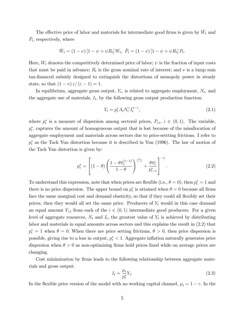
state, so that (1− ν) "/ ("− 1) = 1.In equilibrium, aggregate gross output, Yt, is related to aggregate employment, Nt, and

the aggregate use of materials, It, by the following gross output production function:

Yt = p∗tAtN

γt I

1−γt , (2.1)

where p∗t is a measure of dispersion among sectoral prices, Pi,t, i 2 (0, 1). The variable,p∗t , captures the amount of homogeneous output that is lost because of the misallocation of

aggregate employment and materials across sectors due to price-settting frictions. I refer to

p∗t as the Tack Yun distortion because it is described in Yun (1996). The law of motion of

the Tack Yun distortion is given by:

p∗t =

2

4(1− θ)

1− θπ̄

("−1)t

1− θ

! ""−1

+θπ̄"tp∗t−1

3

5−1

. (2.2)

To understand this expression, note that when prices are flexible (i.e., θ = 0), then p∗t = 1 and

there is no price dispersion. The upper bound on p∗t is attained when θ = 0 because all firms

face the same marginal cost and demand elasticity, so that if they could all flexibly set their

prices, then they would all set the same price. Producers of Yt would in this case demand

an equal amount Yi,t from each of the i 2 (0, 1) intermediate good producers. For a givenlevel of aggregate resources, Nt and It, the greatest value of Yt is achieved by distributing

labor and materials in equal amounts across sectors and this explains the result in (2.2) that

p∗t = 1 when θ = 0. When there are price setting frictions, θ > 0, then price dispersion is

possible, giving rise to a loss in output, p∗t < 1. Aggregate inflation naturally generates price

dispersion when θ > 0 as non-optimizing firms hold prices fixed while on average prices are

changing.

Cost minimization by firms leads to the following relationship between aggregate mate-

rials and gross output:

It =µtp∗tYt. (2.3)

In the flexible price version of the model with no working capital channel, µt = 1− γ. In the

5

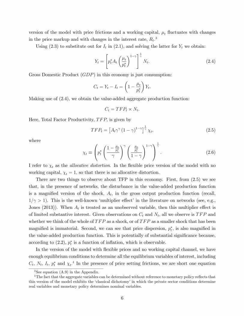
version of the model with price frictions and a working capital, µt fluctuates with changes

in the price markup and with changes in the interest rate, Rt.3

Using (2.3) to substitute out for It in (2.1), and solving the latter for Yt we obtain:

Yt =

"p∗tAt

(µtp∗t

)1−γ# 1γ

Nt. (2.4)

Gross Domestic Product (GDP ) in this economy is just consumption:

Ct = Yt − It =(1−

µtp∗t

)Yt.

Making use of (2.4), we obtain the value-added aggregate production function:

Ct = TFPt ×Nt.

Here, Total Factor Productivity, TFP, is given by

TFPt =[Atγ

γ (1− γ)1−γ] 1γ χt, (2.5)

where

χt ≡

0

@p∗t

1− µt

p∗t

γ

!γ µtp∗t

1− γ

!1−γ1

A

1γ

. (2.6)

I refer to χt as the allocative distortion. In the flexible price version of the model with no

working capital, χt = 1, so that there is no allocative distortion.

There are two things to observe about TFP in this economy. First, from (2.5) we see

that, in the presence of networks, the disturbance in the value-added production function

is a magnified version of the shock, At, in the gross output production function (recall,

1/γ > 1). This is the well-known ‘multiplier e§ect’ in the literature on networks (see, e.g.,

Jones (2013)). When At is treated as an unobserved variable, then this multiplier e§ect is

of limited substantive interest. Given observations on Ct and Nt, all we observe is TFP and

whether we think of the whole of TFP as a shock, or of TFP as a smaller shock that has been

magnified is immaterial. Second, we can see that price dispersion, p∗t , is also magnified in

the value-added production function. This is potentially of substantial significance because,

according to (2.2), p∗t is a function of inflation, which is observable.

In the version of the model with flexible prices and no working capital channel, we have

enough equilibrium conditions to determine all the equilibrium variables of interest, including

Ct, Nt, It, p∗t and χt.4 In the presence of price setting frictions, we are short one equation

3See equation (A.9) in the Appendix.4The fact that the aggregate variables can be determined without reference to monetary policy reflects that

this version of the model exhibits the ‘classical dichotomy’ in which the private sector conditions determinereal variables and monetary policy determines nominal variables.

6

for determining these variables. I fill this gap in the standard way, with a Taylor rule for

setting the nominal rate of interest:

Rt/R = (Rt−1/R)ρ exp

[(1− ρ) 1.5(π̄t − 1.0251/4)

], (2.7)

where R denotes the value of Rt in the non-stochastic steady state. We posit an inflation

target of 2.5 percent per year and that the weight on inflation is 1.5, a value that easily

satisfies the well-known Taylor principle which requires that the weight on inflation exceed

unity.

3. Networks, Price Frictions and the Welfare Cost of Inflation

According to the New Keynesian model described in the previous section, inflation reduces

social welfare by creating relative price distortions which in turn lead to a misallocation of

resources. The resulting loss of output is measured by χt in (2.6). This section shows that

the losses are quantitatively large, particularly when I take into account the network nature

of production.

It is particularly interesting to assess the cost of the high inflation in 1970s and early

1980s because there is a widespread view that that inflation was at least in part responsible

for the poor performance of output and productivity during the period.5 At the same time,

economists have not been successful at identifying a mechanism by which inflation can have

quantitatively large, negative economic e§ects. I show here that when networks are combined

with price-setting frictions as in the previous section, we do have such a mechanism.

The first subsection examines the distortions using steady state calculations. The steady

state has the advantage that it is characterized by simple, transparent expressions. The

second subsection reports a time series on the distortions. Both sets of distortions convey

the same message: the distortions from inflation are quantitatively large, especially when

network e§ects are taken into account.5The American public appears to believe that the 1970s inflation is at least partially responsible for the

poor economic performance of the 1970s. This can be inferred from revealed preference. It is widely believedthat the severe recession of the early 1980s was brought about by Federal Reserve Chairman Paul Volckeras a side-e§ect of his strategy for ending the high inflation of the 1970s. Despite the perceived high cost ofVolcker’s anti-inflation policy, his public reputation is very high. I infer that the public views the benefit ofVolcker’s strategy - ridding the economy of high inflation - is preferred to the cost - the punishing recessionof the early 1980s. That is, the public assigns a high cost to inflation.

7

3.1. Steady State Distortions

Consumer price inflation from 1972Q1 to 1982Q4 averaged 8 percent, at an annual rate.6

One way to evaluate implications of this level of inflation for χt is to compute the steady

state value of p∗ when inflation is 2 percent per quarter. The steady state value of p∗ is,

according to (2.2),

p∗ =1− θπ̄"

(1− θ)(1−θπ̄("−1)

1−θ

) ""−1. (3.1)

The calculation relevant for the period, 1972Q1-1982Q4 uses π̄ = 1.02. In addition, I set

θ = 3/4, which implies that prices are constant on average for one year. I also require a

value for the elasticity of demand, ". The results are dependent on the value assigned to

the elasticity of demand, ", and this is not surprising. The greater that elasticity is, the

greater is the response of resource allocations to a given distortion in relative prices.7 As a

baseline, I follow Christiano, Eichenbaum and Evans (2005) by using " = 6, which implies

a steady state price markup of 20 percent. I also allow for a greater amount of competition

by considering a price markup of 15 percent, which requires " = 7.7.

Results are reported in Table 1. When I evaluate (3.1) in the baseline case, I obtain

p∗ = 0.97. In the case of greater competition, I obtain p∗ = 0.96. Thus, the output loss is

3 percent and 4 percent, respectively, in the baseline and higher competition cases, when

we ignore network e§ects, i.e., γ = 1. To take into account network e§ects, I measure

the distortion by (p∗)1/γ .8 To see the impact of raising p∗ to the power, 1/γ, express p∗ as

p∗ = 1− !. Then, to a first order approximation,

(p∗)1γ ' 1−

1

γ!. (3.2)

From this, we see that the e§ect of introducing networks, i.e., increasing γ from 1 to 2,

roughly doubles the magnitude of the distortion measured in terms of !. Thus, when there

are network e§ects, γ = 2, the loss of output is 5 percent and 9 percent, respectively, in the

baseline and higher competition cases. These are big numbers, hard to ignore.

A possible source of concern about the preceding analysis has to do with the value that I

used for the frequency of price changes, θ. That value is based on studies of US data under

moderate inflation. A natural question is, “was the frequency of price changes in the 1970s

6Here and below, I use data on the consumer price index, CPIAUCSL, taken from the FRED database,maintained by the Federal Reserve Bank of St. Louis.

7There is another e§ect that is dominated in practice by the one cited in the text. In particular, thegreater is the elasticity of substitution between goods, the less severe are the consequences of a given degreeof misallocation.

8I have ignored another channel by which p∗ a§ects, χ (see (3.1)). However, p∗ has both a positive andnegative e§ect on χ by that channel and the two roughly cancel.

8

much higher than it was during periods of more moderate inflation in the US?” The empirical

results reported in Golosov and Lucas (2007) suggest that the answer to the question is ‘no’.

They summarize empirical evidence on the frequency of price adjustment (see their Figure

3) which indicates that a change in inflation from 2.5 percent per year to 10 percent per year

is associated with virtually no change in the frequency of price changes.

3.2. Dynamic Distortions

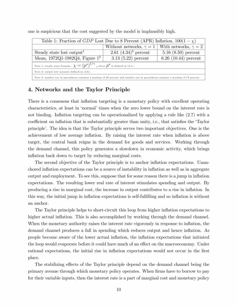
Next, we turn to the time series evidence on p∗t and χt displayed in Figure 1. The objects

that determine these variables are not fully observable. In the case of p∗t I require an initial

condition (see (2.2)). However, I found that the initial condition has a negligible dynamic

e§ect on p∗t . Figure 1 reports the time series on p∗t when the initial value of p

∗t (in 1947Q3) is

set to unity. The results after 1960 are essentially unchanged if I instead choose a far smaller

value of 0.80 for the initial p∗t .

To compute χt I need time series data on µt in addition to p∗t (see (2.6)). In Figure 1 I

simply approximate µt by 1 − γ, its value when prices are flexible and there is no working

capital channel. To investigate the quantitative magnitude of the distortions implied by

this approximation, I did stochastic simulations of the model (see the model details in the

appendix) and found that replacing the actual value of µt with 1−γ has virtually no impacton χt. The reason is that µt enters χt with both a positive and negative sign (see (2.6)).

Figure 1 has two panels. Figure 1a displays results for the baseline parameterization

reported above, in which the markup is 20 percent. Figure 2b reports results for slightly

greater competition, with a markup of 15 percent. Each panel displays three time series:

quarterly observations on quarterly gross inflation in the consumer price index; quarterly

observations on p∗t and quarterly observations on χt. Consider the top panel first. There are

several notable results. First, the output lost implied by the results (!t in (3.2)) is roughly

twice as large when the network structure of production is taken into account (i.e., γ = 2).

Second, the output losses are quantitatively large. The average value of χt is 0.98 so that

on average 2 percent of GDP is lost. Also, 10% of the time, the amount of output lost

exceeds 4.5 percent of GDP . Finally, the losses during the high inflation of the 1970s are

quantitatively large. Indeed, they reach a maximum value of 14 percent in 1979 (see Figure

1).

In the case of increased competition the losses are even larger. Clearly, this model has no

trouble rationalizing the view that high inflation imposes a big cost on society. If anything,

9

one is suspicious that the cost suggested by the model is implausibly high.

Table 1: Fraction of GDP Lost Due to 8 Percent (APR) Inflation, 100(1− χ)Without networks, γ = 1 With networks, γ = 2

Steady state lost output1 2.61 (4.34)3 percent 5.16 (8.50) percentMean, 1972Q1-1982Q4, Figure 12 3.13 (5.22) percent 6.26 (10.44) percent

Note 1: steady state formula - χ = (p∗)1/γ , where p∗ is defined in (3.1).

Note 2: output lost m easure defined in (2.6).

Note 3: number not in parentheses assum es a markup of 20 p ercent and number not in parentheses assum es a markup of 15 p ercent.

4. Networks and the Taylor Principle

There is a consensus that inflation targeting is a monetary policy with excellent operating

characteristics, at least in ‘normal’ times when the zero lower bound on the interest rate is

not binding. Inflation targeting can be operationalized by applying a rule like (2.7) with a

coe¢cient on inflation that is substantially greater than unity, i.e., that satisfies the ‘Taylor

principle’. The idea is that the Taylor principle serves two important objectives. One is the

achievement of low average inflation. By raising the interest rate when inflation is above

target, the central bank reigns in the demand for goods and services. Working through

the demand channel, this policy generates a slowdown in economic activity, which brings

inflation back down to target by reducing marginal costs.

The second objective of the Taylor principle is to anchor inflation expectations. Unan-

chored inflation expectations can be a source of instability in inflation as well as in aggregate

output and employment. To see this, suppose that for some reason there is a jump in inflation

expectations. The resulting lower real rate of interest stimulates spending and output. By

producing a rise in marginal cost, the increase in output contributes to a rise in inflation. In

this way, the initial jump in inflation expectations is self-fulfilling and so inflation is without

an anchor.

The Taylor principle helps to short-circuit this loop from higher inflation expectations to

higher actual inflation. This is also accomplished by working through the demand channel.

When the monetary authority raises the interest rate vigorously in response to inflation, the

demand channel produces a fall in spending which reduces output and hence inflation. As

people become aware of the lower actual inflation, the inflation expectations that initiated

the loop would evaporate before it could have much of an e§ect on the macroeconomy. Under

rational expectations, the initial rise in inflation expectations would not occur in the first

place.

The stabilizing e§ects of the Taylor principle depend on the demand channel being the

primary avenue through which monetary policy operates. When firms have to borrow to pay

for their variable inputs, then the interest rate is a part of marginal cost and monetary policy

10

also operates through a working capital channel. If the working capital channel is su¢ciently

important then, instead of curbing inflation, a jump in the nominal rate of interest could

actually ignite inflation.

Whether the working capital or demand channel dominate has been studied extensively

in the type of model described in the previous section (see, for example, CTW). The general

finding is that when γ = 1 the demand channel dominates the working capital channel and

the Taylor principle achieves the two objectives described above. This is so, even when

the working capital channel is strongest, with = 1. When gross output and value added

coincide, there is not enough borrowing for the working capital channel to overwhelm the

demand channel. However, when we take into account the network nature of production

(i.e., γ = 2), then the amount of borrowing for working capital purposes is potentially much

greater. As a result, when = 1 and there is no interest rate smoothing in the Taylor

rule, i.e., ρ = 0, the non-stochastic steady state equilibrium is indeterminate. Even though

monetary policy satisfies the Taylor principle, there are many equilibria. These equilibria can

be characterized in terms of the loop from higher expected inflation to higher actual inflation

discussed above. When there is no working capital channel, then the Taylor principle short-

circuits this loop by raising the interest rate and preventing the rise in expected inflation

from occurring. But, when the working capital channel is su¢ciently strong, then the rise in

the interest rate simply reinforces the loop from higher expected inflation to higher actual

inflation. In this way the Taylor principle could become the ‘Taylor curse’ referred to in the

introduction.

It is interesting that the Taylor principle works as hoped for when there is substantial

interest rate smoothing in monetary policy, i.e., ρ is large. Presumably, the intuition for this

is that demand responds most strongly to long term interest rates rather than to short term

interest rates. As a result, the strength of the demand channel is increasing in ρ while the

working capital channel, which is only a function of the short term interest rate, remains

una§ected. The example highlights how the integration of network e§ects could be important

for the design of monetary policy. This is a topic that deserves further study. It is important

to know, for example, how pervasive working capital is in the data.9 It is also important to

understand better how the working capital channel works in network environments that are

closer to the more realistic one advocated in the Acemoglu et al paper, in which firms buy

materials directly from other firms.

9For one revelant study, see Barth and Ramey (2002).

11

A. Appendix: Model Used in the Analysis

This comment makes use of a standard New Keynesian model, extended to include network

e§ects following the suggestion of Basu (1995). At the level of detail, the model corresponds

to the one analyzed in CTW. I include a description of the model here for completeness and

because CTW do not describe all the connections between gross output and value-added

that I need for my discussion. Stochastic simulations of the model are used in the discussion

in section 3 and section 4 studies the determinacy properties of the model non-stochastic

steady state.

A.1. Households

There are many identical, competitive households who maximize utility,

maxE0

1X

t=0

βt(u (Ct)−

N1+'t

1 + '

), u (Ct) ≡ logCt,

subject to the following budget constraint:

s.t. PtCt +Bt+1 ≤ WtNt +Rt−1Bt + Profits net of taxest.

Here, Ct denotes consumption; Wt denotes the nominal wage rate; Nt denotes employment;

Pt denotes the nominal price of consumption; Bt+1 denotes a nominal one period bond

purchased in period t which pays o§ a gross, nominal non-state contingent return, Rt, in

period t + 1. Also, the household earns lump sum profits and pays lump sum taxes to the

government. Optimization by households implies:

1

Ct= βEt

1

Ct+1

Rtπ̄t+1

(A.1)

CtN't =

Wt

Pt. (A.2)

A.2. Goods Production

The structure of production has the Dixit-Stiglitz structure that is standard in the New

Keynesian literature, extended to consider network e§ects.

A.2.1. Homogeneous Goods

A representative, homogenous good firm produces output, Yt, using the following technology:

Yt =

[Z 1

0

Y"−1"

i,t dj

] ""−1

, " > 1. (A.3)

12

The firm takes the price of homogeneous goods, Pt, and the prices of intermediate goods,

Pi,t, as given and maximizes profits,

PtYt −Z 1

0

Pi,tYi,tdj,

subject to (A.3). Optimization leads to the following first order condition:

Yi,t = Yt

(PtPi,t

)", (A.4)

for all i 2 (0, 1) . Combining the first order condition with the production function, we obtainthe following equilibrium condition:

Pt =

(Z 1

0

P(1−")i,t di

) 11−"

. (A.5)

A.2.2. Intermediate Goods

The intermediate good, i 2 (0, 1) , is produced by a monopolist using the following technol-ogy:

Yi,t = AtNγi,tI

1−γi,t , 0 < γ ≤ 1.

Here, Ni,t and Ii,t denotes the quantity of labor and materials, respectively, used by the ith

producer. The producer obtains Ii,t by purchasing the homogenous good, Yt, and converting

it one-for-one into materials. Both Ni,t and Ii,t are acquired in competitive markets.

Firms experience Calvo-style frictions in setting their price. That is, the ith firm sets its

period t price, Pi,t, as follows:

Pi,t =

{P̃t with probability 1− θPi,t−1 with probability θ

, 0 ≤ θ < 1. (A.6)

Here, P̃t denotes the price selected in the probability 1− θ event that it can choose its price.Firms that cannot optimize their price must simply set it to whatever value it took on in

the previous period.

Given its current price (however arrived at), the firm must satisfy the Yit that is implied

by (A.4). Linear homogeneity of its technology and our assumption that the ith firm acquires

materials and labor in competitive markets implies that marginal cost is independent of Yi,t.

By studying its cost minimization problem we find that st, the ith firm’s marginal cost (scaled

by Pt) is

st =

(P̄t/Pt1− γ

)1−γ (W̄t/Ptγ

)γ1

At. (A.7)

13

Here, P̄t and W̄t denote the net price, after taxes and interest rate costs, of materials and

labor, respectively. In particular,

W̄t = (1− ν) (1− + Rt)Wt

P̄t = (1− ν) (1− + Rt)Pt,

where, ν is a subsidy selected by the government to extinguish the distortions due to

monopoly power in steady state:10

(1− ν)"

"− 1= 1.

Also, represents the fraction of input costs that must be financed in advance so that, for

example, one unit of labor used during period t costs WtRt units of currency at the end of

the period.11 Another implication of the ith firm’s cost minimization problem is that cost of

materials, P̄tIi,t, as a fraction of total cost, is equal to 1− γ. This implies,

Ii,t = µtYi,t, (A.8)

where µt is the share of materials in gross output, and:

µt =(1− γ) st

(1− ν) (1− + Rt). (A.9)

I now turn to the problem of one of the 1 − θ randomly selected firms that has an

opportunity to select its price, P̃t, in period t. Such a firm is concerned about the value of

its cash flow (i.e., revenues net of costs) in period t and in later periods:

Et

1X

j=0

(βθ)j υt+j

hP̃tYi,t+j − Pt+jst+jYi,t+j

i+ Φt. (A.10)

The objects in square brackets are the cash flows in current and future states in which the firm

does not have an opportunity to reset its price. The expectation operator in (A.10) integrates

over aggregate uncertainty, while the firm-level idiosyncratic uncertainty is manifest in the

presence of θ in the discounting. In (A.10), cash flows in each period are weighed by the

associated date and state-contingent value that the household assigns to cash. The firm

takes these weights as given and

υt+j =u0 (Ct+j)

Pt+j. (A.11)

10The fiscal authority levies lump sum taxes in the amount, ν [(1− + Rt)WtNt + (1− + Rt)PtIt] ,on households.

11We assume that banks create credits which they provide in the amount, ( WtNt + PtIt) , to firms atthe beginning of the period. At the end of the period they receive Rt ( WtNt + PtIt) back from firms andthe profits, (Rt − 1) ( WtNt + PtIt) , are transferred to households in lump sum form.

14

The second term in (A.10), Φt, represents the value of cash flow in future states in which

the firm is able to reset its price. Given the structure of our environment, Φt is not a§ected

by the choice of P̃t. The problem of a firm that is able to choose its price is to select a value

of P̃t that maximizes (A.10) subject to (A.4), taking P̄t, W̄t, Pt and Wt as given.

To solve the firm problem I first substitute out for Yi,t and υt using (A.4) and (A.11),

respectively. I then di§erentiate (A.10) taking into account that Φt is independent of P̃t.

The solution to this problem is obtained by a standard set of manipulations. In particular,

let

p̃t ≡P̃tPt, π̄t ≡

PtPt−1

, Xt,j =

{ 1π̄t+j π̄t+j−1···π̄t+1

, j ≥ 11, j = 0.

,

Xt,j = Xt+1,j−11

π̄t+1, j > 0

Then, the (scaled by Pt) solution to the firm problem is:

p̃t =EtP1

j=0 (βθ)j (Xt,j)

−" Yt+jCt+j

""−1st+j

EtP1

j=0 (βθ)j (Xt,j)

1−" Yt+jCt+j

=Kt

Ft, (A.12)

where

Kt ="

"− 1YtCtst + βθEt

(1

π̄t+1

)−"Kt+1 (A.13)

Ft =YtCt+ βθEt

(1

π̄t+1

)1−"Ft+1. (A.14)

A.3. Economy-wide Variables and Equilibrium

By the usual result associated with Calvo-sticky prices, we have the following cross-price

restriction:

Pt =

(Z 1

0

P(1−")i,t di

) 11−"

=h(1− θ) P̃

(1−")t + θP

(1−")t−1

i 11−". (A.15)

Dividing by Pt and rearranging,

p̃t =

"1− θπ̄

("−1)t

1− θ

# 11−"

. (A.16)

Combining this expression with (A.12), we obtain a useful equilibrium condition:

Kt

Ft=

"1− θπ̄

("−1)t

1− θ

# 11−"

. (A.17)

15

It is convenient to express real marginal cost, (A.7), in terms that do not involve prices:

st = (1− ν)

(1− + Rt

1− γ

)1−γ(A.18)

×(1− + Rt

γCtN

't

)γ1

At,

where (A.2) has been used to substitute out for Wt/Pt.

We now seek the relationship between Gross Domestic Product (GDP ) and aggregate

employment, Nt. To this end, we first compute the equilibrium relationship between aggre-

gate inputs, It and Nt, and gross output, Yt.We do this by adapting an argument suggested

in Yun (1996). We then adapt a version of the argument in Jones (2013) to obtain the

mapping from aggregate employment to GDP.

Let Y ∗t denote the unweighted sum of Yi,t and then substitute out for Yi,t in terms of

prices using (A.4):

Y ∗t ≡Z 1

0

Yi,tdi = Yt

Z 1

0

(Pi,tPt

)−"di = Yt

(PtP ∗t

)",

where

P ∗t ≡[Z 1

0

P−"i,t di

]−1"

=h(1− θ) P̃−"t + θ

(P ∗t−1

)−"i−1", (A.19)

using the analog of the result in (A.15). In this way, we obtain the following expression for

Yt :

Yt = p∗tY∗t , p

∗t ≡

(P ∗tPt

)",

p∗t =

{≤ 1 not Pi,t = Pj,t, all i, j= 1 Pi,t = Pj,t, all i, j

.

We refer to p∗t as the Tack Yun distortion.

By a standard calculation, I obtain the law of motion for p∗t by dividing (A.19) by P∗t ,

using (A.16) and rearranging,

p∗t =

2

4(1− θ)

1− θπ̄

("−1)t

1− θ

! ""−1

+θπ̄"tp∗t−1

3

5−1

. (A.20)

Then,

Yt = p∗tY∗t = p

∗t

Z 1

0

Yi,tdi = p∗tAt

Z 1

0

Nγi,tI

1−γi,t di

= p∗tAt

(NtIt

)γIt,

16

where I have used the fact that all firms have the same materials to labor ratio. In this way,

we obtain

Yt = p∗tAtN

γt I

1−γt . (A.21)

I substitute out for It in (A.21) by noting from (A.8) that

It ≡Z 1

0

Ii,tdi = µt

Z 1

0

Yi,tdi = µtY∗t =

µtp∗tYt. (A.22)

Use this to solve out for It in (A.21):

Yt =

p∗tAt

(µtp∗t

)1−γ! 1γ

Nt. (A.23)

GDP for this economy is simply

Ct = Yt − It. (A.24)

I conclude,

GDPt = Yt − It =(1−

µtp∗t

)Yt = TFPt ×Nt, (A.25)

after some rearranging. Here, TFP denotes total factor productivity and is given by:

TFPt =

p∗tAt

(1−

µtp∗t

)γ (µtp∗t

)1−γ! 1γ

. (A.26)

There are two features of (A.26) worth stressing. First, note that At is raised to the power,

1/γ, so that when γ < 1 the e§ect of a technology shock is magnified by the network e§ects.

This is an illustration of the ‘multiplier e§ect’ emphasized in that literature (see, e.g., Jones,

2013).

Second, note that network e§ects also magnify the e§ects of the Tack Yun distortion.

In standard analyses of the New Keynesian model, which ignore networks (i.e., γ = 1), p∗tis often assumed to be unity. This is justified by the usual practice of setting γ = 1 and

linearizing the model about a steady state with no price distortions, so that p∗t = 1. Given

my assumption of zero price indexation, this requires that there be no inflation in steady

state. It is easy to verify that the first order Taylor series expansion of p∗t about p∗t−1 = 1

and π̄t = 1 is given by:

p∗t = 1 + 0× π̄t + θ(p∗t−1 − 1

).

Evidently, to a first order approximation p∗t converges to unity and shocks (which can only

impact p∗t via their e§ect on π̄t) have no e§ect on p∗t . The practice of linearizing about a

steady state undistorted by price dispersion presumably reflects the conjecture that if the

17

steady state were distorted then the fluctuations in p∗t would be negligibly small. But, even

if the distortions were small in the production of gross output, they may nevertheless be

non-negligible for value-added because of the multiplier e§ects associated with networks.

Thus, if we express p∗t = 1− !t, where !t is a small positive number, then

(p∗t )1γ ' 1−

1

γ!t.

Evidently, p∗t enters (A.26) not just by way of (p∗t )1/γ , but also via µt/p

∗t . However,

stochastic simulation of the model suggest that p∗t has only a small e§ect via that avenue,

essentially because p∗t has both a positive and negative e§ects on it.

To explore the multiplier e§ect of misallocation due to price frictions, p∗t , it is convenient

to identify the biggest that TFP can feasibly be for given Nt. This is the value of TFP

associated with p∗t = 1 and µt/p∗t = γ. Multiplying and dividing (A.26) by this maximum, I

obtain the following decomposition of TFP:

TFPt = χt(Atγ

γ (1− γ)1−γ) 1γ ,

where

χt ≡

0

@p∗t

1− µt

p∗t

γ

!γ µtp∗t

1− γ

!1−γ1

A

1γ

. (A.27)

There are 12 variables to be determined for the model:

Kt, Ft, π̄t, p∗t , st, Ct, Yt, Nt, It, µt, Rt,χt.

There are 11 equilibrium conditions implied by private sector decisions : (A.13), (A.14),

(A.17), (A.20), (A.1), (A.21), (A.24), (A.23), (A.18), (A.9), (A.27). In the special case of

flexible prices, no working capital and an e¢cient subsidy for monopoly power:

θ = 0, I = N = 0,"

"− 1(1− ν) = 1,

then the model dichotomizes. In this case, equilibrium consumption and employment solve

the following two equations:

Nt = 1, Ct =[At (γ)

γ (1− γ)1−γ] 1γ .

In the case that is of interest in this discussion, we need an additional equation to solve the

model variables. To this end, I adopt the following specification of monetary policy:

Rt/R = (Rt−1/R)0.8 exp

h(1− 0.8) 1.5(π̄t − 1.025

14 )i,

18

where R denotes the steady state value of Rt. According to this specification, the target

inflation rate is 1.0062, or 2.5 at an annual rate. The smoothing parameter, 0.8, is large as

it is generally found in the empirical literature. Under my specification, the Taylor principle

is satisfied because the coe¢cient on inflation, 1.5, is well above unity. It can be verified

that the steady state of the model is determinate when the smoothing parameter is 0.8 but

indeterminate when the smoothing parameter is zero. The reasons for this are discussed in

the text.

To compute the dynamic properties of the model I solve the model using second order

perturbation (with pruning), using Dynare.12 For this, I require the model steady state in

which the shocks, at, are held at their steady state values of zero. This steady state is easy

to solve in closed form.

The parameter values I assign to the model are as follows:

π̄ = 1.02514 , = 1, γ =

1

2, β = 1.03−0.25,

θ = 0.75, " = 6

("

"− 1= 1.2

), ' = 1, ν =

1

".

The time series representation I use for at is that it is roughly a first order autoregression in

its first di§erence. In particular,

at = (ρ1 + ρ2) at−1 − ρ1ρ2at−2 + "t, E"2t = 0.01

2,

where ρ1 = 0.99 and ρ2 = 0.3.

References

[1] Barth III, M.J., Ramey, V.A., 2002, ‘The cost channel of monetary transmission,’ in

Bernanke, B., Rogo§, K.S., editors, NBER Macroeconomics Annual 2001, MIT Press,

Cambridge, MA, pp. 199—256.

[2] Basu, S., 1995, ‘Intermediate goods and business cycles: Implications for productivity

and welfare,’ American Economic Review, 85 (3), 512—531.

[3] Calvo, Guillermo A., 1983, ‘Staggered Prices in a Utility-maximizing Framework,’ Jour-

nal of Monetary Econonomics 12 (3), 383—398.

[4] Christiano, Lawrence J., Martin Eichenbaum and Charles Evans, 2005, ‘Nominal Rigidi-

ties and the Dynamic E§ects of a Shock to Monetary Policy,’ Journal of Political Econ-

omy, 113 (1), 1—45.

12The code is available on my website.

19

[5] Christiano, Lawrence J., Cosmin Ilut, Roberto Motto and Massimo Rostagno, 2010,

‘Monetary Policy and Stock Market Booms,’ in Federal Reserve Bank of Kansas City

Economic Policy Symposium in Jackson Hole, Wyoming, Macroeconomic Challenges:

The Decade Ahead.

[6] Christiano, Lawrence J., Mathias Trabandt, and Karl Walentin, 2011, ‘DSGEModels for

Monetary Policy Analysis,’ In Benjamin M. Friedman, and Michael Woodford, editors:

Handbook of Monetary Economics, Vol. 3A, The Netherlands: North-Holland, 2011, pp.

285-367.

[7] Eichenbaum, Martin, Nir Jaimovich, and Sergio Rebelo, 2011, ‘Reference Prices and

Nominal Rigidities,’ American Economic Review 101 (1): 234—62.

[8] Golosov, Mikhail and Robert E. Lucas, Jr., 2007, ‘Menu Costs and Phillips Curves,’

Journal of Political Economy, vol. 115, no. 2.

[9] Jones, Chad, 2013, ‘Misallocation, Economic Growth, and Input-Output Economics,’

in D. Acemoglu, M. Arellano, and E. Dekel, Advances in Economics and Econometrics,

Tenth World Congress, Volume II, Cambridge University Press.

[10] Long, John B. and Charles I. Plosser, 1983, ‘Real Business Cycles,’ Journal of Political

Economy, vol. 91, no. 1.

[11] Yun, Tack, 1996, ‘Nominal Price Rigidity, Money Supply Endogeneity, and Business

Cycles,’ Journal of Monetary Economics, 37 (2), 345—370.

20

1950 1960 1970 1980 1990 2000 2010

0.9

0.95

1

Figure 1a: Graph of Quarterly, Gross US CPI inflation, p-star and chi, assumed markup is 1.2

US CPI inflationp-starChi

1950 1960 1970 1980 1990 2000 2010

0.8

0.85

0.9

0.95

1

Figure 1b: Graph of Quarterly, Gross US CPI inflation, p-star and chi, assumed markup is 1.15

US CPI inflationp-starChi