1 1

1 12009-09-29 13:11:30 UTC / rev b19331f50bbd

Discrete-time Signals and Systems

2 2

2 2

ii

2009-09-29 13:11:30 UTC / rev b19331f50bbd

3 3

3 32009-09-29 13:11:30 UTC / rev b19331f50bbd

Discrete-time Signals and Systems

An Operator Approach

Sanjoy Mahajan and Dennis FreemanMassachusetts Institute of Technology

4 4

4 42009-09-29 13:11:30 UTC / rev b19331f50bbd

Typeset in Palatino and Euler by the authors using ConTEXt and PDFTEX

C© Copyright 2009 Sanjoy Mahajan and Dennis Freeman

Source revision: b19331f50bbd (2009-09-29 13:11:30 UTC)

Discrete-time Signals and Systems by Sanjoy Mahajan and Dennis Freeman(authors) and ?? (publisher) is licensed under the . . . license.

5 5

5 52009-09-29 13:11:30 UTC / rev b19331f50bbd

Brief contents

Preface ix

1 Difference equations 1

2 Difference equations and modularity 17

3 Block diagrams and operators: Two new representations 33

4 Modes 51

5 Repeated roots 63

Bibliography 71

Index 73

6 6

6 6

vi

2009-09-29 13:11:30 UTC / rev b19331f50bbd

7 7

7 72009-09-29 13:11:30 UTC / rev b19331f50bbd

Contents

Preface ix

1 Difference equations 11.1 Rabbits 21.2 Leaky tank 71.3 Fall of a fog droplet 111.4 Springs 14

2 Difference equations and modularity 172.1 Modularity: Making the input like the output 172.2 Endowment gift 212.3 Rabbits 25

3 Block diagrams and operators: Two new representations 333.1 Disadvantages of difference equations 343.2 Block diagrams to the rescue 353.3 The power of abstraction 403.4 Operations on whole signals 413.5 Feedback connections 453.6 Summary 49

4 Modes 514.1 Growth of the Fibonacci series 524.2 Taking out the big part from Fibonacci 554.3 Operator interpretation 574.4 General method: Partial fractions 59

5 Repeated roots 635.1 Leaky-tank background 645.2 Numerical computation 655.3 Analyzing the output signal 67

8 8

8 8

viii

2009-09-29 13:11:30 UTC / rev b19331f50bbd

5.4 Deforming the system: The continuity argument 685.5 Higher-order cascades 70

Bibliography 71

Index 73

9 9

9 92009-09-29 13:11:30 UTC / rev b19331f50bbd

Preface

This book aims to introduce you to a powerful tool for analyzing and de-signing systems – whether electronic, mechanical, or thermal.

This book grew out of the ‘Signals and Systems’ course (numbered 6.003)that we have taught on and off to MIT’s Electrical Engineering and Com-puter Science students.

The traditional signals-and-systems course – for example [16] – empha-sizes the analysis of continuous-time systems, in particular analog circuits.However, most engineers will not specialize in analog circuits. Rather, dig-ital technology offers such vast computing power that analogy circuits areoften designed through digital simulation.

Digital simulation is an inherently discrete-time operation. Furthermore,almost all fundamental ideas of signals and systems can be taught usingdiscrete-time systems. Modularity and multiple representations , for ex-ample, aid the design of discrete-time (or continuous-time) systems. Simi-larly, the ideas for modes, poles, control, and feedback.

Furthermore, by teaching the material in a context not limited to circuits,we emphasize the generality of these tools. Feedback and simulation aboundin the natural and engineered world, and we would like our students to beflexible and creative in understanding and designing these systems.

Therefore, we begin our ‘Signals and Systems’ course with discrete-timesystems, and give our students this book. A fundamental difference frommost discussions of discrete-time systems is the approach using operators.Operators make it possible to avoid the confusing notion of ‘transform’. In-stead, the operator expression for a discrete-time system, and the system’simpulse response are two representations for the same system; they arethe coordinates of a point as seen from two different coordinate systems.Then a transformation of a system has an active meaning: for example,composing two systems to build a new system.

10 10

10 10

x Preface

2009-09-29 13:11:30 UTC / rev b19331f50bbd

How to use this book

Aristotle was tutor to the young Alexander of Macedon (later, the Great).As ancient royalty knew, a skilled and knowledgeable tutor is the mosteffective teacher [3]. A skilled tutor makes few statements and asks manyquestions, for she knows that questioning, wondering, and discussing pro-mote long-lasting learning. Therefore, questions of two types are inter-spersed through the book:

questions marked with a in the margin: These questions are what a tutormight ask you during a tutorial, and ask you to work out the next stepsin an analysis. They are answered in the subsequent text, where you cancheck your solutions and my analysis.

numbered questions: These problems, marked with a shaded background,are what a tutor might ask you to take home after a tutorial. They givefurther practice with the tool or ask you to extend an example, use severaltools together, or resolve paradoxes.

Try lots of questions of both types!

Copyright license

This book is licensed under the . . . license.

Acknowledgments

We gratefully thank the following individuals and organizations:

For suggestions and discussions: . . .

For the free software for typesetting: Donald Knuth (TEX); Han The Thanh(PDFTEX); Hans Hagen and Taco Hoekwater (ConTEXt); John Hobby (Meta-Post); Andy Hammerlindl, John Bowman, and Tom Prince (asymptote);Richard Stallman (emacs); the Linux and Debian projects.

11 11

11 112009-09-29 13:11:30 UTC / rev b19331f50bbd

1Difference equations

1.1 Rabbits 21.2 Leaky tank 71.3 Fall of a fog droplet 111.4 Springs 14

The world is too rich and comlex for our minds to grasp it whole, for ourminds are but a small part of the richness of the world. To cope with thecomplexity, we reason hierarchically. We divide the world into small, com-prehensible pieces: systems. Systems are ubiquitious: a CPU, a memorychips, a motor, a web server, a jumbo jet, the solar system, the telephonesystem, or a circulatory system. Systems are a useful abstraction, chosenbecause their external interactions are weaker than their internal interac-tions. That properties makes independent analysis meaningful.

Systems interact with other systems via forces, messages, or in general viainformation or signals. ‘Signals and systems’ is the study of systems andtheir interaction.

This book studies only discrete-time systems, where time jumps ratherthan changes continuously. This restriction is not as severe as its seems.First, digital computers are, by design, discrete-time devices, so discrete-time signals and systems includes digital computers. Second, almost allthe important ideas in discrete-time systems apply equally to continuous-time systems.

Alas, even discrete-time systems are too diverse for one method of analy-sis. Therefore even the abstraction of systems needs subdivision. The par-ticular class of so-called linear and time-invariant systems admits power-ful tools of analysis and design. The benefit of restricting ourselves to such

12 12

12 12

2 1.1 Rabbits

2009-09-29 13:11:30 UTC / rev b19331f50bbd

systems, and the meaning of the restrictions, will become clear in subse-quent chapters.

1.1 Rabbits

Here is Fibonacci’s problem [6, 10], a famous discrete-time, linear, time-invariant system and signal:

A certain man put a pair of rabbits in a place surrounded on all sides by a wall.How many pairs of rabbits can be produced from that pair in a year if it issupposed that every month each pair begets a new pair which from the secondmonth on becomes productive?

1.1.1 Mathematical representation

This system consists of the rabbit pairs and the rules of rabbit reproduction.The signal is the sequence f where f[n] is the number of rabbit pairs atmonth n (the problem asks about n = 12).

What is f in the first few months?

In month 0, one rabbit pair immigrates into the system: f[0] = 1. Let’sassume that the immigrants are children. Then they cannot have their ownchildren in month 1 – they are too young – so f[1] = 1. But this pair is anadult pair, so in month 2 the pair has children, making f[2] = 2.

Finding f[3] requires considering the adult and child pairs separately (hier-archical reasoning), because each type behaves according to its own repro-duction rule. The child pair from month 2 grows into adulthood in month3, and the adult pair from month 2 begets a child pair. So in f[3] = 3: twoadult and one child pair.

The two adult pairs contribute two child pairs in month 4, and the onechild pair grows up, contributing an adult pair. So month 4 has five pairs:two child and three adult pairs. To formalize this reasoning process, definetwo intermediate signals c and a:

c[n] = number of child pairs at month n;

a[n] = number of adult pairs at month n.

The total number of pairs at month n is f[n] = c[n] + a[n]. Here is a tableshowing the three signals c, a, and f:

13 13

13 13

1 Difference equations 3

2009-09-29 13:11:30 UTC / rev b19331f50bbd

n 0 1 2 3

c 1 0 1 1a 0 1 1 2

f 1 1 2 3

The arrows in the table show how new entries are constructed. An upwarddiagonal arrow represents the only means to make new children, namelyfrom last month’s adults:

a[n − 1] → c[n] or c[n] = a[n − 1].

A horizontal arrow represents one contribution to this month’s adults, thatadults last month remain adults: a[n − 1] → a[n]. A downward diagonalarrow represents the other contribution to this month’s adults, that lastmonth’s children grow up into adults: c[n−1] → a[n]. The sum of the twocontributions is

a[n] = a[n − 1] + c[n − 1].

What is the difference equation for f itself?

To find the equation for f, one has at least two methods: logical deduction(Problem 1.1) or trial and error. Trial and error is better suited for findingresults, and logical deduction is better suited for verifying them. Therefore,using trial and error, look for a pattern among addition samples of f:

n 0 1 2 3 4 5 6

c 1 0 1 1 2 3 5a 0 1 1 2 3 5 8

f 1 1 2 3 5 8 13

What useful patterns live in these data?

One prominent pattern is that the signals c, a, and f look like shifted ver-sions of each other:

a[n] = f[n − 1];

c[n] = a[n − 1] = f[n − 2].

Since f[n] = a[n] + c[n],

14 14

14 14

4 1.1 Rabbits

2009-09-29 13:11:30 UTC / rev b19331f50bbd

f[n] = f[n − 1] + f[n − 2].

with initial conditions f[0] = f[1] = 1.

This mathematical description, or representation, clarifies a point that isnot obvious in the verbal description: that the number of rabbit pairs inany month depends on the number in the two preceding months. Thisdifference equation is said to be a second-order difference equation. Sinceits coefficients are all unity, and the signs are positive, it is the simplestsecond-order difference equation. Yet its behavior is rich and complex.

Problem 1.1 Verifying the conjectureUse the two intermediate equations

c[n] = a[n − 1],

a[n] = a[n − 1] + c[n − 1];

and the definition f[n] = a[n] + c[n] to confirm the conjecture

f[n] = f[n − 1] + f[n − 2].

1.1.2 Closed-form solution

The rabbit difference equation is an implicit recipe that computes new val-ues from old values. But does it have a closed form: an explicit formulafor f[n] that depends on n but not on preceding samples? As a step to-ward finding a closed form, let’s investigate how f[n] behaves as n be-comes large.

Does f[n] grow like a polynomial in n, like a logarithmic function of n, or like anexponential function of n?

Deciding among these options requires more data. Here are many valuesof f[n] (starting with month 0):

1, 1, 2, 3, 5, 8, 13, 21, 34, 55, 89, 144, 233, 377, 610, . . .

15 15

15 15

1 Difference equations 5

2009-09-29 13:11:30 UTC / rev b19331f50bbd

lnf

[n]

n

The samples grow quickly. Their growthis too rapid to be logarithmic, unless f[n]

is an unusual function like (log n)20. Theirgrowth is probably also too rapid for f[n]

to be a polynomial in n, unless f[n] isa high-degree polynomial. A likely al-ternative is exponential growth. To testthat hypothesis, use pictorial reasoning by plotting ln f[n] versus n. Theplotted points oscillate above and below a best-fit straight line. Thereforeln f[n] grows almost exactly linearly with n, and f[n] is approximately anexponential function of n:

f[n] ≈ Azn,

where z and A are constants.

n f[n]/f[n − 1]

10 1.6181818181818

20 1.6180339985218

30 1.6180339887505

40 1.6180339887499

50 1.6180339887499

How can z be estimated from f[n] data?

Because the plotted points fall ever closer to thebest-fit line as n grows, the exponential approx-imation f[n] ≈ Azn becomes more exact as n

grows. If the approximation were exact, then f[n]/f[n−

1] would always equal z, so f[n]/f[n−1] becomesan ever closer approximation to z as n increases.These ratios seem to converge to z = 1.6180339887499.Its first few digits 1.618 might be familiar. For a memory amplifier, feedthe ratio to the online Inverse Symbolic Calculator (ISC). Given a number,it guesses its mathematical source. When given the Fibonacci z, the In-verse Symbolic Calculator suggests two equivalent forms: that z is a rootof 1 − x − x2 or that it is φ ≡ (1 +

√5)/2. The constant φ is the famous

golden ratio [5].

n f[n]/f[n − 1]

10 0.72362506926472

20 0.72360679895785

30 0.72360679775006

40 0.72360679774998

50 0.72360679774998

Therefore, f[n] ≈ Aφn. To find the constant ofproportionality A, take out the big part by di-viding f[n] by φn. These ratios hover around0.723 . . ., so perhaps A is

√3 − 1. Alas, exper-

iments with larger values of n strongly suggestthat the digits continue 0.723606 . . . whereas

√3−

1 = 0.73205 . . .. A bit of experimentation orthe Inverse Symbolic Calculator suggests that0.72360679774998 probably originates from φ/

√5.

16 16

16 16

6 1.1 Rabbits

2009-09-29 13:11:30 UTC / rev b19331f50bbd

This conjecture has the merit of reusing the√

5 already contained in the de-finition of φ, so it does not introduce a new arbitrary number. With thatconjecture for A, the approximation for f[n] becomes

f[n] ≈ φn+1

√5

.

How accurate is this approximation?

n r[n]/r[n − 1]

2 −0.61803398874989601

3 −0.61803398874989812

4 −0.61803398874988624

5 −0.61803398874993953

6 −0.61803398874974236

7 −0.61803398875029414

8 −0.61803398874847626

9 −0.61803398875421256

10 −0.61803398873859083

To test the approximation, take out the bigpart by computing the residual:

r[n] = f[n] − φn+1/√

5.

The residual decays rapidly, perhaps expo-nentially. Then r has the general form

r[n] ≈ Byn,

where y and B are constants. To find y,compute the ratios r[n]/r[n − 1]. They con-verge to −0.61803 . . ., which is almost ex-actly 1 − φ or −1/φ. Therefore r[n] ≈ B(−1/φ)n.

What is the constant of proportionality B?

To compute B, divide r[n] by (−1/φ)n. These values, if n is not too large(Problem 1.2), almost instantly settles on 0.27639320225. With luck, thisnumber can be explained using φ and

√5. A few numerical experiments

suggest the conjecture

B =1√5× 1

φ.

The residual becomes

r[n] = −1√5×

(−

1

φ

)n+1

.

The number of rabbit pairs is the sum of the approximation Azn and theresidual Byn:

f[n] =1√5

(φn+1 − (−φ)−(n+1)

).

17 17

17 17

1 Difference equations 7

2009-09-29 13:11:30 UTC / rev b19331f50bbd

How bizarre! The Fibonacci signal f splits into two signals in at least twoways. First, it is the sum of the adult-pairs signal a and the child-pairssignal c. Second, it is the sum f1 + f2 where f1 and f2 are defined by

f1[n] ≡ 1√5φn+1;

f2[n] ≡ −1√5(−1/φ)n+1.

The equivalence of these decompositions would have been difficult to pre-dict. Instead, many experiments and guesses were needed to establishthe equivalence. Another kind of question, also hard to answer, arises bychanging merely the plus sign in the Fibonacci difference equation into aminus sign:

g[n] = g[n − 1] − g[n − 2].

With corresponding initial conditions, namely g[0] = g[1] = 1, the signal g

runs as follows (staring with n = 0):

1, 1, 0, −1, −1, 0, 1,︸ ︷︷ ︸one period

1, 0, −1, −1, 0, . . . .

Rather than growing approximately exponentially, this sequence is exactlyperiodic. Why? Furthermore, it has period 6. Why? How can this periodbe predicted without simulation?

A representation suited for such questions is introduced in ??. For now,let’s continue investigating difference equations to represent systems.

Problem 1.2 Actual residual

lnr[n

]

n

Here is a semilog graph of the absolute resid-ual |r[n]| computed numerically up to n =

80. (The absolute residual is used becausethe residual is often negative and wouldhave a complex logarithm.) It follows thepredicted exponential decay for a while, butthen misbehaves. Why?

1.2 Leaky tank

In the Fibonacci system, the rabbits changed their behavior – grew up orhad children – only once a month. The Fibonacci system is a discrete-time

18 18

18 18

8 1.2 Leaky tank

2009-09-29 13:11:30 UTC / rev b19331f50bbd

system. These systems are directly suitable for computational simulationand analysis because digital computers themselves act like discrete-timesystems. However, many systems in the world – such as piano strings,earthquakes, microphones, or eardrums – are naturally described as continuous-time systems.

h

leak

To analyze continuous-time systems using discrete-timetools requires approximations. These approximations areillustrated in the simplest interesting continuous-time sys-tem: a leaky tank. Imagine a bathtub or sink filled to aheight h with water. At time t = 0, the drain is openedand water flows out. What is the subsequent height ofthe water?

At t = 0, the water level and therefore the pressure is at its highest, so thewater drains most rapidly at t = 0. As the water drains and the level falls,the pressure and the rate of drainage also fall. This behavior is captured bythe following differential equation:

dh

dt= −f(h),

where f(h) is an as-yet-unknown function of the height.

Finding f(h) requires knowing the geometry of the tub and piping andthen calculating the flow resistance in the drain and piping. The simplestmodel for resistance is a so-called linear leak: that f(h) is proportional toh. Then the differential equation simplifies to

dh

dt∝ −h.

What are the dimensions of the missing constant of proportionality?

The derivative on the left side has dimensions of speed (height per time),so the missing constant has dimensions of inverse time. Call the constant1/τ, where τ is the time constant of the system. Then

dh

dt= −

h

τ.

19 19

19 19

1 Difference equations 9

2009-09-29 13:11:30 UTC / rev b19331f50bbd

R

C

VAn almost-identical differential equation describes thevoltage V on a capacitor discharging across a resistor:

dV

dt= −

1

RCV.

It is the leaky-tank differential equation with time con-stant τ = RC.

Problem 1.3 Kirchoff’s lawsUse Kirchoff’s laws to verify this differential equation.

Approximating the continuous-time differential equation as a discrete-timesystem enables the system to be simulated by hand and computer. In adiscrete-time system, time advances in lumps.

If the lump size, also known as the timestep, is T , then h[n] is the discrete-time approximation of h(nT). Imagine that the system starts with h[0] =

h0. What is h[1]? In other words, what is the discrete-time approximationfor h(T)? The leaky-tank equation says that

dh

dt= −

h

τ.

At t = 0 this derivative is −h0/τ. If dh/dt stays fixed for a whole timestep– a slightly dubious but simple assumption – then the height falls by ap-proximately h0T/τ in one timestep. Therefore

h[1] = h0 −T

τh0 =

(1 −

T

τ

)h[0].

Using the same assumptions, what is h[2] and, in general, h[n]?

The reasoning to compute h[1] from h[0] applies when computing h[2]

from h[1]. The derivative at n = 1 – equivalently, at t = T – is −h[1]/τ.Therefore between n = 1 and n = 2 – equivalently, between t = T andt = 2T – the height falls by approximately −h[1]T/tau,

h[2] = h1 −T

τh1 =

(1 −

T

τ

)h[1].

This pattern generalizes to a rule for finding every h[n]:

h[n] =

(1 −

T

τ

)h[n − 1].

20 20

20 20

10 1.2 Leaky tank

2009-09-29 13:11:30 UTC / rev b19331f50bbd

This implicit equation has the closed-form solution

h[n] = h0

(1 −

T

τ

)n

.

How closely does this solution reproduce the behavior of the original, continuous-time system?

The original, continuous-time differential equation dh/dt = −htau issolved by

h(t) = h0e−t/τ.

At the discrete times t = nT , this solution becomes

h(t) = h0e−nT/τ = h0

(e−T/τ

)n

.

The discrete-time approximation replaces e−T/τ with 1 − T/τ. That differ-ence is the first two terms in the Taylor series for e−T/τ:

e−T/τ = 1 −T

τ+

1

2

(T

τ

)2

−1

6

(T

τ

)3

+ . . . .

Therefore the discrete-time approximation is accurate when the higher-order terms in the Taylor series are small – namely, when T/τ � 1.

This method of solving differential equations by replacing them with discrete-time analogs is known as the Euler approximation, and it can be used tosolve equations that are very difficult or even impossible to solve analyti-cally.

Problem 1.4 Which is the approximate solution?

n

Here are unlabeled graphs showing the discrete-time sam-ples h[n] and the continuous-time samples h(nT), for n =

0 . . . 6. Which graph shows the discrete-time signal?

Problem 1.5 Large timestepsSketch the discrete-time samples h[n] in three cases: (a.) T =

τ/2 (b.) T = τ (c.) T = 2τ (d.) T = 3τ

Problem 1.6 Tiny timestepsShow that as T → 0, the discrete-time solution

21 21

21 21

1 Difference equations 11

2009-09-29 13:11:30 UTC / rev b19331f50bbd

h[n] = h0

(1 −

T

τ

)n

.

approaches the continuous-time solution

h(t) = h0e−nT/τ.

How small does T have to be, as a function of n, in order that the two solutionsapproximately match?

1.3 Fall of a fog droplet

The leaky tank (Section 1.2) is a first-order system, and its differential equa-tion and difference equation are first-order equations. However, the phys-ical world is often second order because Newton’s second law of motion,F = ma, contains a second derivative.

For such systems, how applicable is the Euler approximation? To illustratethe issues that arise in applying the Euler approximation to second-ordersystems, let’s simulate the fall of a fog droplet acted on by gravity (F = mg)and air resistance. A fog droplet is small enough that its air resistance isproportional to velocity rather than to the more usual velocity squared.Then the net downward force on the droplet is mg − bv, where v is itsvelocity and b is a constant that measures the strength of the drag. In termsof position x, with the positive direction as downward, Newton’s secondlaw becomes

md2x

dt2= mg − b

dx

dt.

Dividing both sides by m gives

d2x

dt2= g −

b

m

dx

dt.

What are the dimensions of b/m?

The constant b/m turns the velocity dx/dt into an acceleration, so b/m hasdimensions of inverse time. Therefore rewrite it as 1/τ, where τ ≡ m/b isa time constant. Then

d2x

dt2= g −

1

τ

dx

dt.

22 22

22 22

12 1.3 Fall of a fog droplet

2009-09-29 13:11:30 UTC / rev b19331f50bbd

What is a discrete-time approximation for the second derivative?

In the leaky-tank equation,

dh

dt= −

h

τ,

the first derivative at t = nT had the Euler approximation (h[n + 1] −

h[n])/T and h(t = nT) became h[n]. The second derivative d2x/dt2 is thelimit of a difference of two first derivatives. Using the Euler approximationprocedure, approximate the first derivatives at t = nT and t = (n + 1)T :

dx

dt

∣∣∣t=nT

≈ x[n + 1] − x[n]

T;

dx

dt

∣∣∣t=(n+1)T

≈ x[n + 2] − x[n + 1]

T.

Then

d2x

dt2

∣∣∣t=nT

≈ 1

T

(x[n + 2] − x[n + 1]

T−

x[n + 1] − x[n]

T

).

This approximation simplifies to

d2x

dt2

∣∣∣t=nT

≈ 1

T 2(x[n + 2] − 2x[n + 1] + x[n]) .

The Euler approximation for the continuous-time equation of motion isthen

1

T 2(x[n + 2] − 2x[n + 1] + x[n]) = g −

1

τ

(x[n + 1] − x[n]

T

)or

x[n + 2] − 2x[n + 1] + x[n] = gT 2 −T

τ(x[n + 1] − x[n]).

Our old friend from the leaky tank, the ratio T/τ, has reappeared in thisproblem. To simplify the subsequent equations, define α ≡ T/τ. Thenafter collecting the like terms, the difference equation for the falling fogdroplet is

x[n + 2] = (2 − α)x[n + 1] − (1 − α)x[n] + gT 2.

23 23

23 23

1 Difference equations 13

2009-09-29 13:11:30 UTC / rev b19331f50bbd

As expected, this difference equation is second order. Like the previoussecond-order equation, the Fibonacci equation, it needs two initial values.Let’s try x[−1] = x[0] = 0. Physically, the fog droplet starts from rest at thereference height 0, and at t = 0 starts feeling the gravitational force mg.

For a typical fog droplet with radius 10 µm, the physical paramters are:

m ∼ 4.2 ·10−12 kg;

b ∼ 2.8 ·10−9 kg s−1;

τ ∼ 1.5 ·10−3 s−1.

0

10

20

x[n

](µ

m)

0 10 20n

Relative to τ, the timestep T should be small, oth-erwise the simulation error will large. A timestepsuch as 0.1 ms is a reasonable compromise be-tween keeping reducing the error and speedingup the simulation. Then the dimensionless ratioα is 0.0675. A simulation using these paramtersshows x initially rising faster than linearly, probably quadratically, thenrising linearly at a rate of roughly 1.5 µm per timestep or 1.5 cm s−1.

This simulation result explains the longevity of fog. Fog is, roughly speak-ing, a cloud that has sunk to the ground. Imagine that this cloud reachesup to 500 m (a typical cloud thickness). Then, to settle to the ground, thecloud requires

tfall ∼500 m

1.5 cm s−1∼ 9 hours.

In other words, fog should last overnight – in agreement with experience!

Counting timesteps How many timesteps would the fog-droplet simulation re-quire (with T = 0.1 ms) in order for the droplet to fall 500 m in the simulation?How long would your computer, or another easily available computer, require tosimulate that many timesteps?

Problem 1.7 Terminal velocityBy simulating the fog equation

x[n + 2] = (2 − α)x[n + 1] − (1 − α)x[n] + gT2.

with several values of T and therefore α, guess a relation between g, T , α, and theterminal velocity of the particle.

24 24

24 24

14 1.4 Springs

2009-09-29 13:11:30 UTC / rev b19331f50bbd

1.4 Springs

Now let’s extend our simulations to the most important second-order sys-tem: the spring. Springs are a model for a vast number of systems in thenatural and engineered worlds: planetary orbits, chemical bonds, solids,electromagnetic radiation, and even electron–proton bonds. Since colorrsults from electromagnetic radiation meeting electron–proton bonds, grassis green and the sky is blue because of how springs interact with springs.

km

x

The simplest spring system is a mass connected to a springand free to oscillate in just one dimension. Its differentialequation is

md2x

dt2+ kx = 0,

where x is the block’s displacement from the equilibrium position, m is theblock’s mass, and k is the spring constant. Dividing by m gives

d2x

dt2+

k

mx = 0.

Defining the angular frequency ω ≡√

k/m gives the clean equation:

d2x

dt2+ ω2x = 0.

Now divide time into uniform steps of duration T , and replace the secondderivative d2x/dt2 with a discrete-time approximation:

d2x

dt2

∣∣∣t=nT

≈ x[n + 2] − 2x[n + 1] + x[n]

T 2,

where as usual the sample x[n] corresponds to the continuous-time signalx(t) at t = nT . Then

x[n + 2] − 2x[n + 1] + x[n]

T 2+ ω2x[n] = 0

or after collecting like terms,

x[n + 2] = 2x[n + 1] −(1 + (ωT)2

)x[n].

Defining α ≡ ωT ,

x[n + 2] = 2x[n + 1] −(1 + α2

)x[n].

25 25

25 25

1 Difference equations 15

2009-09-29 13:11:30 UTC / rev b19331f50bbd

This second-order difference equation needs two initial values. A simplepair is x[0] = x[1] = x0. This choice corresponds to pulling the mass right-wards by x0, then releasing it at t = T . What happens afterward?

x

t

To simulate the system numerically, oneshould choose T to make α small. As areasonable small α, try 100 samples peroscillation period: α = 2π/100 or roughly0.06. Alas, the simulation predicts thatthe oscillations grow to infinity.

What went wrong?

Perhaps α, even at 0.06, is too large. Here are two simulations with smallervalues of α:

x

t

x

t

α ≈ 0.031 α ≈ 0.016

These oscillations also explode. The only difference seems to be the rate ofgrowth (Problem 1.8).

Problem 1.8 Tiny values of α

Simulate

x[n + 2] = 2x[n + 1] −(1 + α2

)x[n]

using very small values for α. What happens?

An alternative explanation is that the discrete-time approximation of thederivative caused the problem. If so, it would be surprising, because thesame approximation worked when simulating the fall of a fog droplet. Butlet’s try an alternative definition: Instead of defining

dx

dt

∣∣∣t=nT

≈ x[n + 1] − x[n]

T,

try the simple change to

dx

dt≈ x[n] − x[n − 1]

T.

26 26

26 262009-09-29 13:11:30 UTC / rev b19331f50bbd

Using the same procedure for the second derivative,

d2x

dt2

∣∣∣t=nT

≈ x[n] − 2x[n − 1] + x[n − 2]

T 2.

x

t

The discrete-time spring equation is then

(1 + α2)x[n] = 2x[n − 1] − x[n − 2],

or

x[n] =2x[n − 1] − x[n − 2]

1 + α2.

Using the same initial conditions x[0] = x[1] = 1, what is the subsequenttime course? The bad news is that these oscillations decay to zero!

x

t

However, the good news is that changing the de-rivative approximation can significantly affect thebehavior of the discrete-time system. Let’s try asymmetric second derivative:

d2x

dt2

∣∣∣t=nT

≈ x[n + 1] − 2x[n] + x[n − 1]

T 2.

Then the difference equation becomes

x[n + 2] = (2 − α2)x[n + 1] − x[n].

Now the system oscillates stably, just as a spring without energy loss orinput should behave.

Why did the simple change to a symmetric second derivative solve theproblem of decaying or growing oscillations? The representation of thealternative discrete-time systems as difference equations does not help an-swer that question. Its answer requires the two most important ideas insignals and systems: operators (??) and modes (??).

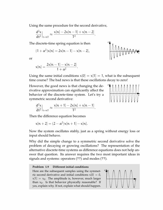
Problem 1.9 Different initial conditionsx

t

Here are the subsequent samples using the symmet-ric second derivative and initial conditions x[0] = 0,x[1] = x0. The amplitude is, however, much largerthan x0. Is that behavior physically reasonable? Ifyes, explain why. If not, explain what should happen.