Discrete surface modelling using partial differential …sequin/CS284/PAPERS/Xu...Discrete surface...

d

s

blems,d in-ons areand gives

s. Theer (sur-ns are

of China

m NIH

Computer Aided Geometric Design 23 (2006) 125–145www.elsevier.com/locate/cag

Discrete surface modelling using partial differential equation

Guoliang Xua,1, Qing Pana, Chandrajit L. Bajajb,∗,2

a State Key Laboratory of Scientific and Engineering Computing, Institute of Computational Mathematics,Academy of Mathematics and System Sciences, Chinese Academy of Sciences, Beijing, 100080, China

b Center for Computational Visualization and Institute for Computational Engineering & Sciences,Department of Computer Science, University of Texas, Austin, TX 78712, USA

Received 29 July 2004; received in revised form 15 May 2005; accepted 23 May 2005

Available online 5 July 2005

Abstract

We use various nonlinear partial differential equations to efficiently solve several surface modelling proincluding surface blending,N -sided hole filling and free-form surface fitting. The nonlinear equations useclude two second order flows, two fourth order flows and two sixth order flows. These nonlinear equatidiscretized based on discrete differential geometry operators. The proposed approach is simple, efficientvery desirable results, for a range of surface models, possibly having sharp creases and corners. 2005 Elsevier B.V. All rights reserved.

Keywords: Free-form surface fitting; Blending;N -sided hole; Differential equations

1. Introduction

We use various partial differential equations (PDE) to solve several surface modelling problemPDEs we use include the mean curvature flow, the averaged mean curvature flow, two fourth ordface diffusion flow and quasi surface diffusion flow) and even higher order flows. All these equatio

* Corresponding author.E-mail address: [email protected] (C.L. Bajaj).

1 Supported in part by Natural Science Foundation of China (10371130) and National Key Basic Research Project(2004CB318000).2 Supported in part by NSF grant ACI-9982297, NSF-ITR grants ACI-0220037 and EIA-03-25550, and a grant fro

R01 GM074258-021.

0167-8396/$ – see front matter 2005 Elsevier B.V. All rights reserved.doi:10.1016/j.cagd.2005.05.004

126 G. Xu et al. / Computer Aided Geometric Design 23 (2006) 125–145

eteriza-g

heslosed byntinuity.curvesce whichity. The

ngu-elling, 1996;n ini-y thebe con-

eviouswithouts timeolution,s a longtable

ld solu-sh. Ineferred

ack tof these

piece of

nonlinear and the geometry is intrinsic, i.e., the PDEs do not depend upon any particular paramtion. The problems we solve include surface blending,N -sided hole filling and free-form surface fittinwith high order boundary continuity.

For the problems of surface blending andN -sided hole filling, we are given triangular surface mesof the surrounding area. Triangular surface patches need to be constructed to fill the openings encthe surrounding surface mesh and interpolate the hole boundary with some specified order of coFor the free-form surface fitting problem, we are possibly given a set of points, or a wire frame ofthat defines an outline of the desired shape, or even some surface patches. We construct a surfainterpolates the points or curves or the boundaries of the patches with specified order of continufree-form surface fitting problem is the most general, including the surface blending andN -sided holefilling problems, as its special cases.

Our twofold strategy for solving these problems is as follows: First we construct an initial trialar surface mesh (“filler”) using any of a number of automatic or semi-automatic free-form modtechniques (see (Bajaj and Ihm, 1992; Bajaj et al., 1993; Greiner, 1994; Peters and WittmanXu et al., 2001)). One may also interactively edit this “filler” to meet the weak assumptions for atial solution shape. This “filler” may be bumpy or noisy, and in general this “filler” does not satisfsmoothness boundary conditions, though it may roughly characterize the shape of the surface tostructed. Second we deform the initial mesh by solving a suitable flow PDE. Unlike most of the prfree-form modelling techniques, our approach solves high-order boundary continuity constraintsany prior estimation of normals or derivative jets along the boundary. The solution of the PDE idependent. We consider two possibilities for the time span of the evolution. One is a short time evwhere we require the solution to respect to the initial shape or geometry (see Fig. 7). The other itime evolution, where the initial filler provides a topological structure, and what we look for is a ssolution state of the flow (see Figs. 1 and 4). In this paper, we focus our attention on these twofotions of PDEs with boundary continuity constraints, rather than the construction of initial filler meSection 3.4, we present automatic approaches for constructing the initial filler mesh, and our prchoice.

Previous work. Earlier research on using PDEs to handle surface modelling problems trace bBloor et al.’s papers at the end of the 1980s (Bloor and Wilson, 1989, 1990). The basic idea o

Fig. 1. (a) shows a head mesh with a hole around the nose. (b) shows an initial filler construction of the nose with aminimal surface. (c) the filler surface, after 30 iteration, generated using fourth order flow (k = 2 in (2.9)) with time step size0.0002. (d) the filler surface, after 20 iteration, generated using sixth order flow (k = 3 in (2.9)) with time step size 0.00002.

G. Xu et al. / Computer Aided Geometric Design 23 (2006) 125–145 127

le fillingereforeon (thethods are

edeickert,x-, 1999;-

ciannsideredemes.lutionobtained and

othing.he mesh

urface

l., 2000)on-

l., 2003;hitakeres (levelrids oflevel-gy (see

ucturesf, 1999))tationalns on

e-formder ands are

used toequationthe

r fairing

papers is the use of biharmonic equations on a rectangular domain to solve the blending and hoproblems. One of the advantages of using the biharmonic equation is that it is linear, and theasier to solve. However, the equation is not geometry intrinsic and the solution of the equatigeometry of the surface) depends on the concrete parameterization used. Furthermore, these meinappropriate to model surfaces with arbitrary shaped boundaries.

The evolution technique, based on the heat equation∂tp − �p = 0, has been extensively usin the area of image processing (see (Preußer and Rumpf, 1999; Weickert, 1998). In (W1998), there are 453 relevant references listed), where� is a 2D Laplace operator. This was etended lately to smoothing or fairing noisy surfaces (see (Clarenz et al., 2000; Desbrun et al.Meyer et al., 2002)). For a surfaceM, the counterpart of the Laplacian� is the Laplace–Beltrami operator �M (see (do Carmo, 1992)). One then obtains the geometric diffusion equation∂tp−�Mp = 0 for asurface pointp(t) on the surfaceM(t). Taubin (1995) discussed the discretized operator of the Laplaand related approaches in the context of generalized frequencies on meshes. Kobbelt (1996) codiscrete approximations of the Laplacian in the construction of fair interpolatory subdivision schThis work was extended in (Kobbelt et al., 1998) to arbitrary connectivity for purposes of multi-resointeractive editing. Desbrun et al. (1999) used an implicit discretization of geometric diffusion toa strongly stable numerical smoothing scheme. The same strategy of discretization is also adoptanalyzed by Deckelnick and Dziuk (2002) with the conclusion that this scheme isunconditionally stable.Clarenz et al. (2000) introduced anisotropic geometric diffusion to enhance features while smoOhtake et al. (2000) combined an inner fairness mechanism in their fairing process to increase tregularity. Bajaj and Xu (2003) smooth both surfaces and functions on surfaces, in aC2 smooth functionspace defined by the limit of triangular subdivision surfaces (quartic Box splines). Similar to the sdiffusion using the Laplacian, a more general class of PDE based methods calledflow surface techniqueshave been developed which simulate different kinds of flows on surfaces (see (Westermann et afor references) using the equation∂tp −V (p, t) = 0, whereV (p, t) represents the instantaneous statiary velocity field.

Level set methods were also used in surface fairing and surface reconstruction (see (Bajaj et aBertalmio et al., 2000; Chopp and Sethian, 1999; Museth et al., 2002; Osher and Fedkiw, 2000; Wand Breen, 1998; Zhao et al., 2000)). In these methods, surfaces are formulated as iso-surfacsurfaces) of 3D functions, which are usually defined from the signed distance over Cartesian ga volume. An evolution PDE on the volume governs the behavior of the level surface. Theseset methods have several attractive features including, ease of implementation, arbitrary topolo(Breen and Whitaker, 2001)) and a growing body of theoretical results. Often, fine surface strare not captured by level sets, although it is possible to use adaptive (see (Preußer and Rumpand triangulated grids as well as Hermite data (see (Kobbelt et al., 2001)). To reduce the compucomplexity, Bertalmio et al. (2000) solve the PDE in a narrow band for deforming vectorial functiosurfaces (with a fixed surface represented by the level surface).

Recently, surface diffusion flow has been used to solve the surface blending problem and fresurface fitting problem (Schneider and Kobbelt, 2000; Schneider and Kobbelt, 2001). In (SchneiKobbelt, 2000), fair meshes withG1 conditions are created in the special case where the mesheassumed to have subdivision connectivity. In this paper, local surface parameterization is stillestimate the surface curvatures. The later paper (Schneider and Kobbelt, 2001) uses the samefor smoothing meshes while satisfyingG1 boundary conditions. Outer fairness (the smoothness inclassical sense) and inner fairness (the regularity of the vertex distribution) criteria are used in thei


uation,ow is

ow) for

t is gen-ults for aermore,

d in thislutionsEs are

ows

locityplace–

nce ands can bett, 1998;face

).uct of a

process. The finite element method is used by Clarenz et al. (2004) to solve the Willmore flow eqbased on a new variational formulation of the flow, for the aim of surface restoration. Willmore flalso used to smooth triangular mesh in (Yoshizawa and Belyaev, 2002).

Main results. We use second order flows (mean curvature flow and averaged mean curvature flG0 continuity, fourth order flows forG1 continuity and sixth order flows forG2 continuity in each ofseveral surface modelling problems. The proposed approach is simple and easy to implement. Ieral, solves several surface modelling problems in the same manner, and gives very desirable resrange of complicated free-form surface models, possibly having sharp features and corners. Furthit avoids the estimation of normals or tangents or curvatures on the boundaries.

The rest of the paper is organized as follows: Section 2 describes several nonlinear PDEs usepaper. In Section 3, we give details of the discretization and the numerical computation for the soof the PDEs. Examples to illustrate the different effects achievable from the solution of the PDgiven in Section 4.

2. Partial differential equation models

Let M be a smooth surface andp ∈M be the surface point. The general form of the geometric flwe consider is in the following form (see (Westermann et al., 2000))

∂p

∂t= V (p, t),

whereV (p, t) ∈ R3 represents a velocity field. We shall focus our attention on using two classes ve

fields, one is curvature driven velocity field in the normal direction, the other is the higher order LaBeltrami operators acting on surface pointp.

2.1. Geometric partial differential equations

We now describe several geometric PDE models we use in this paper. More details on the existeuniqueness of the solutions, the numerical computations of the solutions and evolution behaviorfound in a series of papers by Mayer, Simonett, Escher (Escher et al., 1998; Escher and SimoneSimonett, 2001) and Huiskens’ (1987) paper. LetM0 be a compact closed immersed orientable surin R

3. A curvature driven geometric evolution consists of finding a family{M(t): t � 0} of smoothclosed immersed orientable surfaces inR

3 which evolve according to the flow equation

∂p

∂t= N(p)Vn(k1, k2,p), M(0) = M0. (2.1)

Herep(t) is a surface point onM(t), Vn(k1, k2,p) denotes the normal velocity ofM(t), which dependson the principal curvaturesk1, k2 of M(t), N(p) stands for the unit normal of the surface atp(t). Inthis paper we identify the surface pointp and surface normalN(p) as 3× 1 matrices (column vectorsHence, the arithmetic operations of these quantities are regarded matrix operations. The prodscalara ∈ R and a matrixM is written as eitheraM or Ma.


1))d

ollows

tion

hrinking

Let A(t) denote the area ofM(t), V (t) denote the volume of the region enclosed byM(t). Then ithas been shown that (see (Willmore, 1993, Theorem 4))

dA(t)

dt=

∫M(t)

VnH dσ,dV (t)

dt=

∫M(t)

Vn dσ, (2.2)

whereH = 12(k1 + k2) is the mean curvature ofM(t).

2.1.1. Mean curvature flow (see (Dziuk, 1991; White, 2002))TakingVn = −H = −1

2(k1 + k2) in (2.1), we obtain the mean curvature flow PDE:

∂p

∂t= −N(p)H(p), M(0) = M0. (2.3)

It follows from (2.2) that

dA(t)

dt= −

∫M(t)

H 2 dσ. (2.4)

(2.4) implies that the mean curvature flow is area reducing.

2.1.2. Averaged mean curvature flow (see (Escher and Simonett, 1998; Huiskens, 1987; Sapiro, 200In (2.1), if we takeVn = h(t) − H(t), whereh(t) = ∫

M(t)H dσ/

∫M(t)

dσ , then we have the averagemean curvature flow PDE:

∂p

∂t= N(p)

[h(t) − H(p)

], M(0) = M0. (2.5)

The existence proof of the global solutions to this flow can be found in Huiskens’ (1987) paper. It ffrom (2.2) that

dA(t)

dt=

∫M(t)

(hH − H 2)dσ =∫

M(t)

[hH − H 2 − h(h − H)

]dσ = −

∫M(t)

(h − H)2 dσ � 0, (2.6)

since obviously∫M(t)

h(h−H) = h(h∫M(t)

dσ −∫M(t)

H dσ) = 0. On the other hand, the second equaof (2.2) implies that

dV (t)

dt= h(t)

∫M(t)

dσ −∫

M(t)

H dσ = 0.

Hence the averaged mean curvature flow is volume preserving and area shrinking. The area sstops ifH ≡ h.

2.1.3. Surface diffusion flow (see (Schneider and Kobbelt, 2001))If we takeVn = �H , we get the so-called surface diffusion flow PDE:

∂p = N(p)�H(p), M(0) = M0, (2.7)
∂t


2) and

ting onbut

men-ay not

the vol-t

higheres notesirable

progres-oach is

where� := �M is Laplace–Beltrami operator which acts on functions defined on surfaceM(t). Theexistence and uniqueness of solutions for this flow is given in (Escher et al., 1998). From (2.Green’s formula we have

d

dtA(t) =

∫M(t)

�HH dσ = −∫

M(t)

|∇H |2 dσ � 0,

d

dtV (t) =

∫M(t)

div(∇H)dσ = −∫

M(t)

∇H∇(1)dσ = 0,

where∇ stands for the (tangential) gradient operator (see (do Carmo, 1976, pp. 101–102)) acdifferential functions defined on the surfaceM. Hence, the surface diffusion flow is area shrinking,volume preserving. The area stops shrinking when the gradient ofH is zero. That is,M is a surface withconstant mean curvature.

2.1.4. Higher order geometric flows∂p

∂t= (−1)k+1N(p)�kH(p), M(0) =M0. (2.8)

Using Green formula, we have∫M(t)

�kH dσ =∫

M(t)

�(�k−1H)dσ =∫

M(t)

∇(�k−1H)∇(1)dσ = 0.

Hence, the flow (2.8) is volume preserving ifk � 1 from the second equation of (2.2).

Remark 2.1. We should note that the area/volume preserving/shrinking properties for the flowstioned above are valid for closed surfaces. In our application of these flows, these properties mbe true since the surfaces always have fixed boundaries. For a open surface with fix boundary,umeV (t) could be defined as the directional volume betweenM(0) andM(t). It is easy to see thathe volume preserving property for the averaged mean curvature flow is still valid. But for theorder flow (2.8) (k � 1), this property is no longer valid, because a term related to the boundary dovanish when Green’s formula is used. For our modelling problems, volume preservation is not a dproperty (see Figs. 1 and 4).

Remark 2.2. In (Schneider and Kobbelt, 2001), Schneider and Kobbelt use elliptic equationN(p)�H(p)

= 0, while we use several time dependent parabolic type equations. In our approach, we have asive process starting from an initial value, so that a family of solutions is obtained. Such an apprvery desirable if the initial value is an approximation of the required solution.

2.2. Quasi geometric partial differential equations

Now we generalize the heat equation on a surface to the following higher order flows:

∂p = (−1)k+1�kp, M(0) = M0, k > 0. (2.9)
∂t


ish

the geo-nalysis

is basedlarenz

n finitelrfaces.ow theribed in. Other

ltramive beenper we

h aboutwn thate,

r order

Since�p = −2H(x)N(p), it is easy to see that (2.9) is the mean curvature flow whenk = 1 (up to afactor 2). But since(�kH)N �= �k(HN) in general, (2.9) is different from the flow (2.8). To distinguthe difference between (2.8) and (2.9), we call (2.9) as a quasi geometric PDE.

The experiments conducted in this paper show that flows (2.9) sometimes behave better thanmetric flows mentioned above for our geometry modelling problems. However, the theoretical aon the existence and stability of their solutions is currently unavailable.

3. Solution of the PDEs

There are basically two classes of approaches for solving a PDE on any domain. One approachon finite divided differences, the other is based on finite elements (see (Bajaj and Xu, 2003; Cet al., 2004; Deckelnick and Dziuk, 2002)). The approach we adopt in this paper is based odivided differences. Since we are dealing with differential equations over 2-manifolds inR

3, the classicafinite divided differences will be replaced by discretized differential geometric operators over suSection 3.1 deals with discretized geometric differential operators. Next in Section 3.2 we detail hboundary conditions are respected. Discretizations of the PDEs in the spatial direction are descSections 3.3 and 3.4. Semi-implicit discretization in the time domain is considered in Section 3.5issues, such as mesh regularization and initial mesh construction, are addressed in Section 3.6.

3.1. Discretized Laplace–Beltrami operator

One of the fundamental problems in solving our PDEs is the discretization of the Laplace–Beoperator. On a triangular surface mesh, several discretized approximations of the operator haproposed (see (Desbrun et al., 1999; Guskov et al., 1999; Taubin, 2000; Xu, 2004b)). In this paadopt the discretization developed by Meyer et al. in (Meyer et al., 2002). A comparative researcthe various discretized Laplace–Beltrami operators is conducted in (Xu, 2004a). It has been shothe scheme of Meyer et al.’s is better for discretizing our PDEs. Letf be a smooth function on a surfacthen�f is approximated over a triangular meshM by

�f (pi) ≈ 1

AM(pi)

∑j∈N1(i)

cotαij + cotβij

2

[f (pj ) − f (pi)

], (3.1)

whereN1(i) is the index set of 1-ring of neighbor vertices of vertexpi , αij and βij are the triangleangles shown in Fig. 2 (left).AM(pi) is the area for vertexpi as shown in Fig. 2 (right), whereqj is thecircumcenter point for the triangle[pj−1pjpi] if the triangle is non-obtuse. If the triangle is obtuse,qj

is chosen to be the midpoint of the edge opposite to the obtuse angle. Since�p = −2H(p)N(p) (see(Willmore, 1993, p. 151)), we have

(�p)p=pi= −2H(pi)N(pi) ≈ 1

AM(pi)

∑j∈N1(i)

cotαij + cotβij

2(pj − pi). (3.2)

This gives an approximation of the mean curvature normal (see (Meyer et al., 2002)). The higheLaplace–Beltrami operators are discretized recursively as

�kf (pi) = �(�k−1f )(pi) = 1

AM(pi)

∑ cotαij + cotβij

2

[�k−1f (pj ) − �k−1f (pi)

](3.3)

j∈N1(i)


ofhe

bound-(see

Fig. 2. Left: The definition of the anglesαij andβij . Right: The definition of the areaAM(pi).

Fig. 3. Left: The involved vertices of the “outer” mesh for aG0 boundary condition. The “outer” mesh is just the boundarythe hole. Middle: The involved vertices of the “outer” mesh for aG1 boundary condition. Right: The involved vertices of t“outer” mesh for aG2 boundary condition.

with �0f (pi) = f (pi). Note that�kf (pi) involves function values on ak-ring of neighboring verticesof pi .

3.2. Handling of boundary conditions

3.2.1. Natural boundary conditions for blending and hole fillingBy the natural boundary conditions, we mean that no continuity conditions are specified at the

ary points, but the continuity is implied by the “outer” mesh incident to the boundary of the holeFig. 3). Such a treatment for boundary condition is suitable for both the blending problem and theN -sidedhole filling problem, since the “outer” mesh always exists in such problems.

Let gi be the order of continuity at a boundary pointpi , g = maxgi . Then we can use the order 2g

flow ∂p

∂t= (−1)g+1�gH(p)N(p) for constructing the triangular surface patch withGgi continuity at

the boundary vertexpi . �gH is discretized recursively:�gH = �(�g−1H). At a boundary vertexpi ,�kH(pi) is evaluated according to the following rule:

Evaluation rule at boundary. �kH(pi) is evaluated recursively by formulas (3.6) and (3.7) if k � gi ,otherwise �kH(pi) is set to zero and the recursion stops.


tion of

ices areand side.

ish tod order

ecifiedation is

collectedseveralding to

secondy. Thesestimated

more, the

s

001)).

d

Note that even for an inner vertexpj , the recursive definition may make�kH(pj ) involve the evalua-tion of a lower order Laplace–Beltrami operator on the boundary. In general, the recursive evalua�kH(pi) at pi (for pi either being an inner or an outer vertex) involves(k + 1)-ring neighbor verticesof pi . Some of them may be inner vertices, and the remaining are outer vertices. The inner verttreated as unknowns in the discretized equations and the outers are incorporated into the right-h

3.2.2. Natural boundary conditions for free-form surface fillingIn the free-form surface filling problem, we are given a wireframe of curves (edges) and we w

flesh the wireframe with surface patches that contain the curves as boundary with pre-specifieof continuity. At each of the intersection points of the patches, an order of continuity is pre-spand the evaluation rule mentioned above is applied. For each inner point, a discretized linear equgenerated using the operator discretization (3.7). These linear equations for different patches aretogether and solved simultaneously. Note that one linear equation may involve inner vertices ofpatches. However, if the continuity order at each boundary point is zero, any equation corresponan inner vertex does not involve inner vertices of other patches.

Remark 3.1. Schneider and Kobbelt (2001) use Moreton and Sequin’s least square fitting of thefundamental form relative to a local parameterization to estimate the required data on the boundarestimations of the boundary derivative data are based on incomplete information. Hence, the edata maybe not reliable. Our approach is based on the identity�Mp = −2H(p)N(p). Hence, we donot need to estimate boundary derivative data, such as normals, tangents or curvatures. Furtherboundary conditions are treated in the same way for equations with different orders.

3.3. Spatial discretization of quasi geometric flows

Let us consider first the discretization of (2.9) in the spatial direction fork = 1,2,3. Let P =[p1, . . . , pm]T ∈ R

m×3, �P = [�p1, . . . ,�pm]T ∈ Rm×3, wherep1, . . . , pm are all the unknown vertice

to be determined in each of our modelling problems. Then (3.2) could be written in matrix form:

�P = −(DW)P + B(1), (3.4)

whereD = diag[ 12A(p1)

, . . . , 12A(pm)

] is a diagonal matrix,W = {wij }mi,j=1 with

wij =

∑k∈N1(i)

cotαik + cotβik, i = j,

−(cotαij + cotβij ), i �= j, i ∈ N1(j), j ∈ N1(i),

0, otherwise.

Furthermore,W is a sparse, symmetric and positive definite matrix (see (Schneider and Kobbelt, 2The constant termB(1) ∈ R

m×3 is obtained from the boundary conditions. It follows from (3.4) that

�2P = (DWDW)P + B(2), (3.5)

whereB(2) ∈ Rm×3 is obtained from the boundary conditions. Again,WDW is a sparse, symmetric an

positive definite matrix. In general,

�kP = (−1)k(DW)kP + B(k),

and the matrix forD−1(DW)k is also sparse, symmetric and positive definite.


i-

3.4. Spatial direction discretization of geometric flows

Let

ωij =

∑k∈N1(i)

cotαik+cotβik

2AM(pi), i = j,

− cotαij +cotβij

2AM(pi), i �= j, i ∈ N1(j), j ∈ N1(i),

0, otherwise,

andN(i) = N1(i) ∪ {i}. Then we have

N(pi)H(pi) ≈ 1

2

∑j∈N(i)

ωijpj . (3.6)

The higher order Laplace–Beltrami operators acting onH are discretized recursively as

�kH(pi) = �(�k−1H)(pi) ≈ −∑

j∈N(i)

ωij�k−1H(pj) (3.7)

with

�0H(pi) = H(pi) ≈ 1

2

∑j∈N(i)

ωijN(pi)T pj . (3.8)

Note that�kH(pi) involves values of the mean curvature on ak-ring of neighboring vertices ofpi .Using (3.6)–(3.8) and the evaluation rule at the boundary, we can writeN(pi)�

kH(pi) as the follow-ing form:

N(pi)�kH(pi) ≈ (−1)k

∑j∈J0

ω(k)ij pj + B

(k)i , ω

(k)ij ∈ R

3×3, B(k)i ∈ R

3,

whereJ0 is the index set of the (unknown) vertices to be determined,B(k)i comes from boundary cond

tion. To be more specific, letJ denote the index set of the meshM , Jk be the union ofJ0 and the indexset of the boundary vertices whereCk condition is specified. Then

N(pi)H(pi) ≈ 1

2

∑j∈N(i)

ωijpj = 1

2

∑j∈N(i)∩J0

ωijpj + 1

2

∑j∈N(i)∩{J\J0}

ωijpj

=∑j∈J0

ω(0)ij pj + B

(0)i , (3.9)

whereω(0)ij = 1

2ωij I3 for j ∈ N(i) ∩ J0, ω(0)ij = 0 otherwise,B(0)

i = 12

∑j∈N(i)∩{J\J0} ωijpj . Similarly,

N(pi)�H(pi) ≈ −N(pi)∑

j∈N(i)

ωijH(pj ) = −N(pi)∑

j∈N(i)∩J1

ωijH(pj )

= −N(pi)∑

j∈N(i)∩J1

ωijN(pj )T N(pj )H(pj )

≈ −∑

ωijN(pi)N(pj )T

[∑m

(0)jk pk + B

(0)j

]
j∈N(i)∩J1 k∈J0


f

-

st atr de-ns. Letn as

stemem. The

the

ivening to

er thaneve the

emi-h.

= −∑j∈J0

ω(1)ij pj + B

(1)i , (3.10)

N(pi)�2H(pi) ≈ −N(pi)

∑j∈N(i)

ωij�H(pj ) = −N(pi)∑

j∈N(i)∩J2

ωij�H(pj )

≈ N(pi)∑

j∈N(i)∩J2

ωij

∑k∈N(j)∩J1

ωjkH(pk)

≈∑

j∈N(i)∩J2

∑k∈N(j)∩J1

ωijωjkN(pi)N(pk)T

[∑l∈J0

m(0)kl pl + B

(0)k

]

=∑j∈J0

ω(2)ij pj + B

(2)i . (3.11)

(3.9)–(3.11) are used to discretize the right-handed side of (2.8) fork = 0,1,2. The discretization oN(pi)�

kH(pi) for k > 2 is recursively calculated using (3.7) and boundary conditions.

3.5. Time discretization

Given an approximate solution{p(n)i }mi=1 of the order 2k PDE attn for all the inner vertices, we con

struct an approximate solution{p(n+1)i }mi=1 for the next time steptn+1 = tn + τ (n) by using a semi-implicit

Euler scheme. That is, we replace the derivative∂p

∂twith [p(tn+1) − p(tn)]/τ (n), and the quantitie

wij in (3.4), ωij and N(pi) in (3.6)–(3.8),h(t) in (2.5) are computed using the previous resultn. NormalsN(pi) are computed from Loop’s subdivision surface (see (Bajaj and Xu, 2003) fotail). Such a treatment yields a linear system of equations with the inner vertices as unknowP (n+1) = [(p(n+1)

1 )T , . . . , (p(n+1)m )T ]T ∈ R

3m. The linear system for the geometric flows can be writtethe matrix form[

I + τ (n)W (k)]P (n+1) = B(k), W (k) = {

ω(k)ij

}, B(k) ∈ R

3m. (3.12)

The matrixW (k) ∈ R3m×3m is highly sparse, hence an iterative method for solving such a linear sy

is desirable. We use Saad’s iterative method (Saad, 2000), named GMRES, to solve the systexperiment shows that this iterative method works very well.

Let P (n+1) = [p(n+1)

1 , . . . , p(n+1)m ]T ∈ R

m×3. The linear system for the flows (2.9) can be written asmatrix form[

I + τ (n)(DW)k+1]P (n+1) = B(k), or W(k)P (n+1) = D−1B(k) (3.13)

whereB(k) ∈ Rm×3, W(k) = D−1 + τ (n)W(DW)k ∈ R

m×m is a highly sparse, symmetric and positdefinite matrix, and hence we use a conjugate gradient iterative method with diagonal preconditiosolve the system.

Note that for the same size problem, the size of coefficient matrix in (3.12) is three times largthat of coefficient matrix in (3.13). Furthermore, the matrixW(k) in (3.13) is symmetric and positivdefinite. The matrix in (3.12) is not. We also note that the discretization of (2.9) does not involcomputation of the surface normals.

Remark 3.2. It is well known that the condition of the linear system arising from the proposed simplicit discretization behaves like O(1 + τ (n)h−2k), whereh is the minimal edge length of the mes


uch alieved bymethod,

algebraicntation,

flowevelopinitial

l mesh.re, werity

o occur,point

(3.18)).

nonuni-olution

ent to

Hence, if the mesh to be evolved is very irregular, the resulting system will be ill-conditioned. In scase, a small time step size is required to make an iterative solver converge. Such a problem is rethe mesh regularization treatment (see Section 3.6). On the other hand, more advanced iterativesuch as multi-grid techniques based on a hierarchical mesh representation (see (Lang, 2001)) ormulti-grid techniques, could be used to accelerate the iteration process. In the current implemethese techniques are not incorporated.

Upper-bound of time step. It is known that several surface evolutions (e.g., the mean curvature(see (Dziuk, 1991; White, 2002)) and the surface diffusion flow (see (Bansch et al., 2002))) may dsingularities. For our geometric modelling problems, suppose we have a topologically correctsurface mesh construction and we look for solutions that have the same topology as the initiaHence, we require that our solution is within the time period in that no singularity occurs. Therefoshall determine the time stepτ (n) so thattn should not go beyond the time moment when the singulaoccurs. LetL(p

(n)i ,M(tn)) be the spatial discretization ofV (p, t) at vertexp

(n)i over the meshM(tn).

Then from the approximate equality∥∥p(n+1)i − p

(n)i

∥∥ = τ (n)∥∥L(p

(n)i ,M(tn))

∥∥and the requirement

∥∥p(n+1)i − p

(n)i

∥∥ � 1

2min

j∈N1(i)

∥∥p(n)j − p

(n)i

∥∥ (3.14)

we determine an upper-bound forτ (n) as follows

τ (n) � Bn := 1

2min

1�i�m

{minj∈N1(i) ‖p(n)

j − p(n)i ‖

‖L(p(n)i ,M(tn))‖

}.

Requirement (3.14) guarantees that no vertex-collision happens. When the singularity is nearly tthe upper-boundBn will approach to zero. Hence the evolution cannot move beyond the singularfor time.

Remark 3.3. When the singularity is nearly to occur, the upper-boundBn will approach to zero. Thiswill be a very low efficiency process. So a threshold valueε0 should be put on the minimalBn. If thedeterminedBn is smaller than the threshold value, we terminate the evolution process (see (3.17)–

3.6. Other important issues

3.6.1. Mesh regularizationThe surface motion by the geometric PDEs described in Section 2 may cause a very irregular (

form) distribution of the mesh vertices. Hence, introducing a regularization mechanism in the evprocess is necessary. Sincethe tangential displacement does not influence the geometry of the deforma-tion, just its parameterization (see (Epstein and Gage, 1987)), we also add a tangential displacemthe motion. Hence, the general form of our geometric evolution problem could be written as

∂p = V (p, t) + Vt(p)T (p), M(0) = M0, (3.15)
∂t


ss

ur-e

t isesperty ofe et al.

,

initialomatic, 2002;ller” to

steps.tes or6). Theata to bery dataurfaces.nd then

shouldvelopeddary of

abovefinite

whereT (p) is a tangent direction at the surface pointp, Vt(p) is the tangential velocity. In the proceof numerical solution of Eq. (3.15),Vt(p)T (p) is chosen as

U0(p(n)i ) − (

U0(p(n)i ),N(p

(n)i )

)N(p

(n)i ) (3.16)

whereU0(p(n)i ) = 1

card(N1(i))

∑j∈N1(i)

(p(n)j − p

(n)i ), N is the surface normal computed from the limit s

face of Loop’s subdivision. This discretization ofVt(p)T (p) is very similar to the one given by Ohtaket al. (2000), which isU0(p

(n)i ) − (U0(p

(n)i ),N(p

(n)i ))U0(p

(n)i ). The difference is that our displacemen

in the tangent plane. In (3.16),U0(p(n)i ) could be replaced byU0(p

(n+1)i ) to use as many of the new valu

as possible, and still yield a linear system. However, such a treatment destroys the symmetric prothe coefficient matrix. The tangential motion (3.16) is also used by Wood et al. (2000) and Ohtak(2001).

3.6.2. Stopping criteriaWe need to determine the minimal iteration numbern, so that the evolution procedure stops att = tn.

The following two criteria are used∥∥M(tn) − M(0)∥∥ � ε1 or Bn < ε0 (3.17)∥∥M(tn+1) − M(tn)

∥∥/τ (n) � ε2 or Bn < ε0 (3.18)

whereεi are given control constants,Bn is the determined upper-bound forτ (n). Criterion (3.17) is forshort time evolution, where we requireM(nτ (n)) nearM(0). Criterion (3.18) is for long time evolutionwhere we are looking for a stable status of the solution. ConditionBn < ε0 is imposed for avoidingdead-loop around the singular point of time.

3.6.3. Construction of initial surface meshTo provide an initial solution to the geometric evolution problem, we need to construct an

triangular surface mesh (“filler”) for each opening using any of a number of automatic or semi-autfree-form surface construction techniques (Bajaj and Ihm, 1992; Bajaj et al., 1993; Davis et al.Greiner, 1994; Peters and Wittman, 1996; Xu et al., 2001). One can also interactively edit this “fimeet the weak assumptions for an initial solution shape.

Since the opening to be filled could be topologically complicated, we solve the problem in twoIn the first step we fit each opening by an implicit algebraic surface or spline which interpolaapproximates the boundary data (Bajaj et al., 1993; Bajaj and Xu, 1994; Peters and Wittman, 199approach we used is the one developed by Bajaj et al. (1992, 1993, 1994). In this approach, the dinterpolated or approximated could be points or curves (even with normals). For ours, the boundaare always points. Of course, this approach may not guarantee to produce topologically correct sIf this happens, we break the opening into several parts by inserting a few curves (polygons) arepeat the surface fitting for each part until we achieve a reasonable shape for the “filler”.

After the algebraic surface is obtained, a triangulation step is employed. Since this triangulationbe consistent with the boundary polygon of the opening, we adopted the expansion technique dein (Bajaj and Xu, 1994). Using this approach, we triangulate the surfaces starting from the bounthe opening.

Remark 3.4. Comparing with finite element approach, the finite difference approach describedis easy to implement and it treats the equations with different orders in a uniform fashion. In the


r highernowns,t methodf four

oblemsed by

f Fig. 4effectsuse the

meanith ange therth order

der flow

here (leftl mesh).on

2.8)

element approach, one has to make efforts to derive a variational form for each of the PDEs. Foorder flows, hybrid method is used in general, such an approach will introduce much more unkand therefore the resulted linear system is much larger. For example, in order to use finite elemen(linear element) for the surface diffusion flow, Bänsch et al. (2002) split the PDE into a system oequations.

4. Comparative examples

In this section, we give several examples to show how the PDEs are used to solve different prin a uniform fashion. We also compare the effects of flows (2.8) and (2.9). All the figures producthe fourth and sixth flows are generated using (2.9), except for the figures of the second row oand third row of Fig. 6. These figures are produced using the flow (2.8). When we compare theof (2.8) and (2.9), we use the same number of iterations but double time step size for (2.8) becafactor 2 in the relation�p = −2HN .

4.1. Comparison of the flows

The first three figures of the first row of Fig. 4 show the long time evolution solutions of thecurvature flow, the fourth order flow, and the sixth order flow (2.9) for the input semi-sphere winitial construction of the opening, a triangulated disk. The mean curvature flow does not chandisk. (b) and (c) are the results after 10 iterations withτ (n) = 0.1 andτ (n) = 0.001, respectively. Furtheiterations do not have a significant change on the shape of the solution surface. The fourth and sixflows yield convex surfaces and the smoothness is clearly observed. Also notice that the sixth or

Fig. 4. The first and second row show the results of (2.9) and (2.8), respectively. (a) (same as (g)) The input semi-sppart) with an initial planar triangulation of the disk opening. The mean curvature flow does not change the disk (initia(b) The result of fourth order flow after 10 iteration withτ (n) = 0.1. (c) The result of the sixth order flow after 10 iteratiwith τ (n) = 0.01. (d), (e) and (f) show three intermediate results of the sixth order flow withτ (n) = 0.001, and 1, 6 and 10iterations, respectively. (h) The result of the surface diffusion flow after 10 iteration withτ (n) = 0.2. (i) The result of the sixthorder flow (2.8) after 10 iteration withτ (n) = 0.02. (j), (k) and (l) show three intermediate results of the sixth order flow (with τ (n) = 0.002, and 1, 6 and 10 iterations, respectively.


ow.tively. (c),e set to 0,

xth orderurfacef theely, andth ordera much

for arties are

te thes to bel(e) ands. The000625,

ler timemeshes

Fig. 5. Comparison of different flows.�k represents 2k order flow (2.9) is used.AM denote the averaged mean curvature flThe time step sizes for the second, fourth and sixth order flows are chosen to be 0.1, 0.0025, and 0.0000625, respec(e), (g) are the faired interpolating surface meshes after 6 iterations, where the continuities at the boundary curves ar2 and 0, respectively. (d), (f), (h) are the mean curvature (MC) plots of (c), (e), (g), respectively.

recovers the sphere accurately. The last three figures show three intermediate results of the siflow. The second and third figures of the second row of Fig. 4 show the evolution solutions of the sdiffusion flow and sixth order flows (2.8) for the input semi-sphere with an initial construction oopening. (h) and (i) are produced using the same number of iterations as (b) and (c), respectivdouble time step sizes. Again, the last three figures show three intermediate results of the sixflow. Comparing with the figures of the first row, the geometric flows change the surface shape inslower rate.

Remark 4.1. We have pointed that the geometric flows (2.8) have volume preserving propertiesclosed surface. However, for an open surface with fixed boundary, the volume preserving propenot guaranteed. (h) and (i) show that the volume preserving property is not valid.

Fig. 5 shows the combined use of different flows. The aim of this toy example is to illustradifference of these flows, especially the continuity on the patch boundaries. (a) shows four circleinterpolated. Two of the circles are in thexz-plane, the other two are in theyz-plane. (b) shows an initiaG0 surface mesh constructed using (Bajaj and Ihm, 1992) with some additional noise added. (c),(g) are the faired interpolating surfaces after 6 iterations using different combinations of the flowtime step sizes for the second, fourth and sixth order flows are chosen to be 0.1, 0.0025, and 0.0respectively. Since the higher order flows evolve faster than the lower order flows, we use smalstep sizes for higher order flows to obtain nearly the same surface evolution speed. Each of the


two

(e) and

d meanght partt whileill yieldithe flow.

ooksth order

meshesrs to benalusing theationsturelendingoth

-at the

metriche nosejaj

(d)) arerdervailable

consists of four surface patches. The left two patches are in the regionsR−+ := {(x, y, z): x � 0, y � 0}andR−− := {(x, y, z): x � 0, y � 0}, respectively, and generated by one type of flow. The rightpatches are in the regionsR++ := {(x, y, z): x � 0, y � 0} and R+− := {(x, y, z): x � 0, y � 0},respectively, and generated by a different flow. (d), (f) and (h) are the mean curvature plots of (c),(g), respectively. The mean curvature at each vertex is computed by (3.2).

The aim of (c) is to show the difference between the mean curvature flow and the averagecurvature flow, where the left part is generated by the averaged mean curvature flow and the riis produced by the mean curvature flow. The mean curvature flow shrinks the surface very fasthe averaged mean curvature flow does not. Further evolution using the mean curvature flow wa pinch-off of the surface. Therefore, if we model a surface patch using second order flows wG0

boundary condition, the averaged mean curvature flow is more desirable than the mean curvaturThe patches inR−+ andR−− of (e) are produced by the sixth order flow (2.9) (withk = 3), while

the patches inR++ andR+− are produced by the fourth order flow (2.9). As a whole, the surface lsmooth, our curvature plot reveals the smoothness difference at the intersection curves, the sixflow gives a smoother result than the fourth order flow.

(g) is produced as (e), but the continuity order at the four circles are set to zero. HenceG0 continuityis achieved there.

4.2. Surface blending

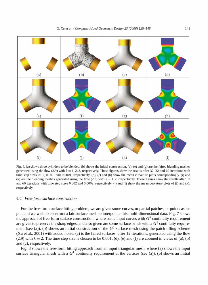
Given a collection surface mesh with boundaries, we construct a fair surface to blend theat the boundaries with specified geometric continuity. Fig. 6 shows the case, where three cylindeblended are given (a) with an initialG0 construction (b) using (Bajaj and Ihm, 1992) with some additionoise added. The blending surfaces (c), (e) and (g) are the faired blending meshes generatedflow (2.9) with k = 1,2,3, respectively. These figures show the results after 32, 32 and 60 iterwith time step sizes 0.01, 0.001, and 0.0001, respectively. (d), (f) and (h) show the mean curvaplots correspondingly. These figures clearly show the difference of smoothness achieved at bboundaries. The mean curvature flow givesG0 continuity results. The fourth order flow produces smosurfaces at boundaries. The sixth order flow produces even smoother surfaces as expected.

(i) and (k) are the faired blending meshes generated using the flow (2.8) withk = 1,2, respectively.These figures show the results after 32 and 60 iterations with time step sizes 0.002 and 0.0002, respectively. (j) and (l) show the mean curvature plots of (i) and (k), respectively. It should be noted thflows (2.9) generate little fatter surface than the flows (2.8).

4.3. N -sided hole filling

Given a surface mesh with a hole, we construct a fair surface to fill the hole with specified geocontinuity on the boundary. Fig. 1 shows such an example, where a head mesh with a hole in tsubregion is given as input (a). An initialG0 reconstruction of the nose is shown in (b) using (Baand Ihm, 1992) and then evolved with the mean curvature flow. The blending surfaces ((c) andgenerated using the flow (2.9) withk = 2 and 3, respectively. It should be observed that the sixth oflow yields a better restoration surface. The head mesh with the hole in the nose subregion is afrom http://lsec.cc.ac.cn/~xuguo/xuguo2.htm.

http://lsec.cc.ac.cn/~xuguo/xuguo2.htm

http://lsec.cc.ac.cn/~xuguo/xuguo2.htm


g meshess withi) andr 32(k),

s as in-shows

t

methe flow(b)

e inputitial

Fig. 6. (a) shows three cylinders to be blended. (b) shows the initial construction. (c), (e) and (g) are the faired blendingenerated using the flow (2.9) withk = 1,2,3, respectively. These figures show the results after 32, 32 and 60 iterationtime step sizes 0.01, 0.001, and 0.0001, respectively. (d), (f) and (h) show the mean curvature plots correspondingly. ((k) are the blending meshes generated using the flow (2.8) withk = 1,2, respectively. These figures show the results afteand 60 iterations with time step sizes 0.002 and 0.0002, respectively. (j) and (l) show the mean curvature plots of (i) andrespectively.

4.4. Free-form surface construction

For the free-form surface fitting problem, we are given some curves, or partial patches, or pointput, and we wish to construct a fair surface mesh to interpolate this multi-dimensional data. Fig. 7the approach of free-form surface construction, where some input curves withG0 continuity requiremenare given to preserve the sharp edges, and also given are some surface bands with aG1 continuity require-ment (see (a)). (b) shows an initial construction of theG0 surface mesh using the patch filling sche(Xu et al., 2001) with added noise. (c) is the faired surfaces, after 12 iterations, generated using(2.9) withk = 2. The time step size is chosen to be 0.001. (d), (e) and (f) are zoomed in views of (a),and (c), respectively.

Fig. 8 shows the free-form fitting approach from an input triangular mesh, where (a) shows thsurface triangular mesh with aG1 continuity requirement at the vertices (see (a)). (b) shows an in


ofafter 12in

es. Therocess.

ure, after 2atureand the

e thornsroblem

as

roblemsduceses thein

ral wayresults

Fig. 7. Interpolating curves and patches: (a) shows some input curves withG0 continuity requirement and some bandsmesh withG1 continuity requirement. (b) shows an initial construction of the surface mesh. (c) is the faired surfaces,iterations, generated using the flow (2.9) withk = 2. The time step size is chosen to be 0.001. (d), (e) and (f) are the zoomresults of (a), (b) and (c), respectively.

construction of the surface mesh, where each input triangle is approximated with 16 sub-trianglnewly introduced vertices are treated as unknowns and the input vertices are fixed in the fairing p(c) and (d) are the faired meshes, after 2 iterations withτ (n) = 0.01, generated using the mean curvatflow and the averaged mean curvature flow, respectively. (e) is the faired mesh by fourth order flowiterations withτ (n) = 0.001. (f) is the mean curvature plot of (e). The area shrinking of the mean curvflow makes the input vertices to be interpolated become thorns (see (c)), while the area shrinkingvolume preservation of the averaged mean curvature flow make some of input vertices becomand some others become pits (see (d)). However, the fourth order flow does not suffer from this p(see (e)). The obtained surface interpolates the input points and exhibitsG1 smoothness everywherewell.

5. Conclusions

We have presented a general scheme for using PDEs to solve several surface modelling pand with high order boundary continuity conditions. Our scheme has the following features: It provery fair and desirable solution surfaces. It is simple and easy to implement. Specifically, it solvfree-form blending problem, theN -sided hole filling problem and free-form surface fitting problema uniform fashion, and solves the high order boundary continuity problem in an easy and natuand avoids prior estimation of normals or derivative jets on the boundaries. The implementation


surfaceged).

rs andually ofcurrenteral

owever,ller and

r their

Fig. 8. Interpolating points: (a) shows some input points and their triangulation. (b) shows an initial construction of themesh. (c) and (d) are the faired surfaces, after 2 iterations withτ (n) = 0.01, using the mean curvature flow and the averamean curvature flow, respectively. (e) is faired surfaces, after 2 iterations withτ (n) = 0.001, using the fourth order flow (2.9(f) is the mean curvature plot of (e).

show that our solution works well for a wide range of surface models. Note that theC1 or higher ordercontinuity interpolatory surface blending solution produced by, e.g., (Bajaj and Ihm, 1992; PeteWittman, 1996) for complicated corners, or holes with many boundary curve segments, are usvery high algebraic degree and thereby prone to be with unsuitable for certain applications. Thesolution of starting withG0 low degree blends, coupled with higher order flow evolution, yields in gena much better alternative for very smooth surface solutions.

Both the geometric flows and quasi geometric flows yield smooth surfaces at the boundaries. Hquasi geometric flows (2.9) have some attractive features, including ease of implementation, smabetter behaved coefficient matrices and no requirement of derivatives (normal) estimation.

Acknowledgement

The authors are grateful to the referees for their carefully reading of the manuscript and fohelpful comments on improving the final version of this paper.


elli, C., Singa-

urfaces.

chnical

al Con-

ns for

sign 21

ed De-

Graph. 7

undary

iz2000,

: Proc.

th. 91,

e flow.

deling,

. 126 (9),

nal. 29

eedings,

eome-

In: SIG-

In: SIG-

References

Bajaj, C., Ihm, I., 1992. Algebraic surface design with Hermite interpolation. ACM Trans. Graph. 19 (1), 61–91.Bajaj, C., Xu, G., 1994. Rational spline approximations of real algebraic curves and surfaces. In: Dikshit, H.P., Mich

(Eds.), Approximations and Decomposition Series. In: Advances in Computational Mathematics. World Scientificpore, pp. 73–85.

Bajaj, C., Xu, G., 2003. Anisotropic diffusion of surface and functions on surfaces. ACM Trans. Graph. 22 (1), 4–32.Bajaj, C., Ihm, I., Warren, J., 1993. Higher order interpolation and least squares approximation using implicit algebraic s

ACM Trans. Graph. 12 (4), 327–347.Bajaj, C., Wu, Q., Xu, G., 2003. Level-set based volumetric anisotropic diffusion for 3D image denoising. ICES Te

Report 03-10, University of Texas at Austin.Bansch, E., Morin, P., Nochetto, R.H., 2002. Finite element methods for surface diffusion. In: Proc. of the Internation

ference on Free Boundary Problems, Theory and Applications, Trento, Italy.Bertalmio, M., Sapiro, G., Cheng, L.T., Osher, S., 2000. A framework for solving surface partial differential equatio

computer graphics applications. CAM Report 00-43, UCLA, Mathematics Department.Bloor, M.I.G., Wilson, M.J., 1989. Generating blend surfaces using partial differential equations. Computer-Aided De

(3), 165–171.Bloor, M.I.G., Wilson, M.J., 1990. Using partial differential equations to generate free-form surfaces. Computer-Aid

sign 22 (4), 221–234.Breen, D., Whitaker, R., 2001. A level-set approach for the metamorphosis of solid models. IEEE Trans. Vis. Comput.

(2), 173–192.do Carmo, M.P., 1976. Differential Geometry of Curves and Surfaces. Prentice-Hall, Englewood Cliffs, NJ.Chopp, D.L., Sethian, J.A., 1999. Motion by intrinsic Laplacian of curvature. Interfaces and Free Boundaries 1, 1–18.Clarenz, U., Diewald, U., Dziuk, G., Rumpf, M., Rusu, R., 2004. A finite element method for surface restoration with bo

conditions. Computer Aided Geometric Design 21 (5), 427–445.Clarenz, U., Diewald, U., Rumpf, M., 2000. Anisotropic geometric diffusion in surface processing. In: Proceedings of V

IEEE Visualization, Salt Lake City, Utah, pp. 397–505.Davis, J., Marschner, S.R., Garr, M., Levoy, M., 2002. Filling holes in complex surfaces using volumetric diffusion. In

First International Symposium on 3D Data Processing, Visualization, Transmission.Deckelnick, K., Dziuk, G., 2002. A fully discrete numerical scheme for weighted mean curvature flow. Numer. Ma

423–452.Desbrun, M., Meyer, M., Schröder, P., Barr, A.H., 1999. Implicit fairing of irregular meshes using diffusion and curvatur

In: SIGGRAPH99, Los Angeles, USA, pp. 317–324.do Carmo, M., 1992. Riemannian Geometry. Boston.Dziuk, G., 1991. An algorithm for evolutionary surfaces. Numer. Math. 58, 603–611.Epstein, C.L., Gage, M., 1987. The curve shortening flow. In: Chorin, A., Majda, A. (Eds.), Wave Motion: Theory, Mo

and Computation. Springer-Verlag, New York.Escher, J., Simonett, G., 1998. The volume preserving mean curvature flow near spheres. Proc. Amer. Math. Soc

2789–2796.Escher, J., Mayer, U.F., Simonett, G., 1998. The surface diffusion flow for immersed hypersurfaces. SIAM J. Math. A

(6), 1419–1433.Greiner, G., 1994. Variational design and fairing of spline surface. Computer Graphics Forum 13, 143–154.Guskov, I., Sweldens, W., Schröder, P., 1999. Mutiresolution signal processing for meshes. In: SIGGRAPH ’99 Proc

pp. 325–334.Huiskens, G., 1987. The volume preserving mean curvature flow. J. Reine Angew. Math. 382, 35–48.Kobbelt, L., 1996. Discrete fairing. In: Goodman, T., Martin, R. (Eds.), The Mathematics of Surfaces VII. Information G

ters, pp. 101–129.Kobbelt, L., Campagna, S., Vorsatz, J., Seidel, H.-P., 1998. Interactive muti-resolution modeling on arbitrary meshes.

GRAPH98, pp. 105–114.Kobbelt, L., Botsch, M., Schwanecke, U., Seidel, H.P., 2001. Feature sensitive surface extraction from volume data.

GRAPH2001, pp. 51–66.


tions.

lds. In:

8.tion. In:

sign 33,

atics of

heories in

ge.ing,

eomet-

, IEEE

national

f Mathe-

dings of

.67–784.etric

Process-

gainzed

Lang, J., 2001. Adaptive Multilevel Solution of Nonlinear Parabolic PDE Systems: Theory, Algorithm, and ApplicaSpringer, Berlin.

Meyer, M., Desbrun, M., Schröder, P., Barr, A., 2002. Discrete differential-geometry operator for triangulated 2-manifoProceedings of Visual Mathematics’02, Berlin, Germany.

Museth, K., Breen, D., Whitaker, R., Barr, A., 2002. Level set surface editing operators. In: SIGGRAPH02, pp. 330–33Ohtake, Y., Belyaev, A.G., Bogaevski, I.A., 2000. Polyhedral surface smoothing with simultaneous mesh regulariza

Geometric Modeling and Processing Proceedings, pp. 229–237.Ohtake, Y., Belyaev, A.G., Bogaevski, I.A., 2001. Mesh regularization and adaptive smoothing. Computer-Aided De

789–800.Osher, S.J., Fedkiw, R.P., 2000. Level set methods. CAM Report 00-07, UCLA, Mathematics Department.Peters, J., Wittman, M., 1996. Smooth blending of basic surfaces using trivariate box spline. In: IMA 96, The Mathem

Surfaces. Dundee, UK.Preußer, T., Rumpf, M., 1999. An adaptive finite element method for large scale image processing. In: Scale-Space T

Computer Vision, pp. 232–234.Saad, Y., 2000. Iterative Methods for Sparse Linear Systems, second edition with corrections.Sapiro, G., 2001. Geometric Partial Differential Equations and Image Analysis. Cambridge University Press, CambridSchneider, R., Kobbelt, L., 2000. Generating fair meshes withG1 boundary conditions. In: Geometric Modeling and Process

Hong Kong, China, pp. 251–261.Schneider, R., Kobbelt, L., 2001. Geometric fairing of irregular meshes for free-form surface design. Computer Aided G

ric Design 18 (4), 359–379.Simonett, G., 2001. The Willmore flow for near spheres. Differential and Integral Equations 14 (8), 1005–1014.Taubin, G., 1995. A signal processing approach to fair surface design. In: SIGGRAPH’95 Proceedings, pp. 351–358.Taubin, G., 2000. Signal processing on polygonal meshes. In: EUROGRAPHICS.Weickert, J., 1998. Anisotropic Diffusion in Image Processing. B.G. Teubner, Stuttgart.Westermann, R., Johnson, C., Ertl, T., 2000. A level-set method for flow visualization. In: Proceedings of Viz2000

Visualization, Salt Lake City, Utah, pp. 147–154.Whitaker, R., Breen, D., 1998. Level set models for the deformation of solid objects. In: Proceedings of the 3rd Inter

Workshop on Implicit Surfaces, Eurographics Association, pp. 19–35.White, B., 2002. Evolution of curves and surfaces by mean curvature. In: Proceedings of the International Congress o

maticians, vol. I, Beijing, pp. 525–538.Willmore, T.J., 1993. Riemannian Geometry. Clarendon Press, Oxford.Wood, Z.J., Breen, D., Desbrun, M., 2000. Semi-regular mesh extraction from volumes. In: IEEE Visualization Procee

the conference on Visualization’00, Salt Lake City, Utah, United States, pp. 275–282.Xu, G., 2004a. Convergence of discrete Laplace–Beltrami operators over surfaces. Comput. Math. Appl. 48, 347–360Xu, G., 2004b. Discrete Laplace–Beltrami operators and their convergence. Computer Aided Geometric Design 21, 7Xu, G., Bajaj, C., Huang, H., 2001.C1 modeling with A-patches from rational trivariate functions. Computer Aided Geom

Design 18 (3), 221–243.Yoshizawa, S., Belyaev, A.G., 2002. Fair triangle mesh generation with discrete elastica. In: Geometric Modeling and

ing, Saitama, Japan, pp. 119–123.Zhao, H.K., Osher, S., Merriman, B., Kang, M., 2000. Implicit and non-parametric shape reconstruction from unor

points using variational level set method. Computer Vision and Image Understanding 80 (3), 295–319.

Discrete surface modelling using partial differential …sequin/CS284/PAPERS/Xu...Discrete surface...

Documents

Transcript of Discrete surface modelling using partial differential …sequin/CS284/PAPERS/Xu...Discrete surface...