Discrete Logarithms on Elliptic Curves
30
Rose-Hulman Undergraduate Mathematics Journal Rose-Hulman Undergraduate Mathematics Journal Volume 12 Issue 1 Article 3 Discrete Logarithms on Elliptic Curves Discrete Logarithms on Elliptic Curves Aaron Blumenfeld University of Rochester, [email protected] Follow this and additional works at: https://scholar.rose-hulman.edu/rhumj Recommended Citation Recommended Citation Blumenfeld, Aaron (2011) "Discrete Logarithms on Elliptic Curves," Rose-Hulman Undergraduate Mathematics Journal: Vol. 12 : Iss. 1 , Article 3. Available at: https://scholar.rose-hulman.edu/rhumj/vol12/iss1/3
Transcript of Discrete Logarithms on Elliptic Curves

Rose-Hulman Undergraduate Mathematics Journal Rose-Hulman Undergraduate Mathematics Journal
Volume 12 Issue 1 Article 3
Discrete Logarithms on Elliptic Curves Discrete Logarithms on Elliptic Curves
Aaron Blumenfeld University of Rochester, [email protected]
Follow this and additional works at: https://scholar.rose-hulman.edu/rhumj
Recommended Citation Recommended Citation Blumenfeld, Aaron (2011) "Discrete Logarithms on Elliptic Curves," Rose-Hulman Undergraduate Mathematics Journal: Vol. 12 : Iss. 1 , Article 3. Available at: https://scholar.rose-hulman.edu/rhumj/vol12/iss1/3
Rose-HulmanUndergraduateMathematicsJournal
Sponsored by
Rose-Hulman Institute of Technology
Department of Mathematics
Terre Haute, IN 47803
Email: [email protected]
http://www.rose-hulman.edu/mathjournal
Discrete Logarithms on EllipticCurves
Aaron Blumenfelda
Volume 12, no. 1, Spring 2011
aUniversity of Rochester, New York, [email protected]

Rose-Hulman Undergraduate Mathematics Journal
Volume 12, no. 1, Spring 2011
Discrete Logarithms on Elliptic Curves
Aaron Blumenfeld
Abstract. Cryptographic protocols often make use of the inherent hardness of theclassical discrete logarithm problem, which is to solve gx ≡ y (mod p) for x. Thehardness of this problem has been exploited in the Diffie-Hellman key exchange, aswell as in cryptosystems such as ElGamal. There is a similar discrete logarithmproblem on elliptic curves: solve kB = P for k. Therefore, Diffie-Hellman andElGamal have been adapted for elliptic curves. There is an abundance of evidencesuggesting that elliptic curve cryptography is even more secure, which means thatwe can obtain the same security with fewer bits. In this paper, we investigate thediscrete logarithm for elliptic curves over Fp for p ≥ 5 by constructing a functionand considering the induced functional graph and the implications for cryptography.
Acknowledgements: The author would like to extend thanks to Joshua Holden for hisadvice and helpful suggestions throughout this project.

RHIT Undergrad. Math. J., Vol. 12, no. 1 Page 31
1 Introduction
The two most studied number theoretic problems in cryptography are factoring integers andsolving the discrete logarithm problem. In this paper, we focus on the latter. The processof modular exponentiation takes a base g (possibly a primitive root) and an integer x andcomputes y = gx mod p. The inverse transformation is known as the discrete logarithmproblem — that is, to solve gx ≡ y (mod p) for x. This is considered one of the hardestproblems in cryptography, and it has led to many cryptographic protocols.
The best known such protocol that employs the hardness of the discrete logarithm prob-lem is the Diffie-Hellman key exchange. In Diffie-Hellman, the two parties, Alice and Bob,agree on a (public) primitive root g and a large prime p. They choose secret integers, a andb, respectively. Then Alice sends ga mod p to Bob, and Bob sends gb mod p to Alice. Thenthey can both compute gab mod p since gab ≡ (ga)b ≡ (gb)a (mod p). They can use this num-ber as their key or use some algorithm to extract a key out of this number. Given ga, gb, gand p, it seems impossible to find gab without finding either a or b, which amounts to solvingthe discrete logarithm problem (although this assertion has not been proved). Similar ideasare the basis of several cryptosystems, the most prominent of which is ElGamal.
In the past several decades, elliptic curves have entered the scene. Elliptic curves overfinite fields contain finite cyclic groups that we can use for cryptography. There is no factor-ization problem for elliptic curves, but what is used is the discrete logarithm problem, whichis to solve kB = P for k. The analog of Diffie-Hellman, in particular, is as follows. Alice andBob choose a public elliptic curve E (including a public prime p that determines Fp) and apublic generator B. They then choose secret integers, a and b, respectively. Alice sends BobaB and Bob sends Alice bB. They can then both compute abB since a(bB) = b(aB) = abB.In this case, abB is a point, so they can use the x-coordinate (or perhaps run it throughsome algorithm) to obtain a key. Similarly, ElGamal and other cryptosystems have beenadapted to elliptic curves.
In this paper, we introduce some of the technical details of elliptic curves over Fp forp ≥ 5 and functional graphs, which we then use to study the discrete logarithm problem onelliptic curves. The ultimate goal is, of course, to show that these cryptographic protocolsare indeed secure. It would make sense that they are secure if discrete “exponentiation”(written additively in this case) behaves like a “random” map. This map is easier to studythrough its associated functional graph. Therefore, we devise a functional graph from ellipticcurve discrete “exponentiation” and consider some of its theoretical properties, as well asobserved computational results.
In particular, we investigate the map k 7→ x(kB),∞ 7→ ∞, where x(P ) denotes thex-coordinate of the point P . We show that these graphs are binary as long as we have Npoints on the curve with N ≥ p odd, and we compare various statistics on these graphs to theexpected asymptotic values for random binary functional graphs. Most of the statistics matchup well. A few statistics deviate because there is a fixed point at infinity by construction.One statistic that deviates that is more difficult to explain, however, is maximum tail length.This seems to suggest some subtle structure in discrete exponentiation. We discuss this and

Page 32 RHIT Undergrad. Math. J., Vol. 12, no. 1
the implications for elliptic curve cryptography in detail in this paper.
2 Background
2.1 Elliptic Curves
Definition 2.1. An elliptic curve E over a field K is the set{(x, y) ∈ K2 : y2 = x3 + ax+ b, a, b ∈ K
}∪ {∞}
with the restriction that 4a3 + 27b2 6= 0. Notationally, once we have specified the field K, werefer to E as E(K).
Technical Point : There is a more general form of the equation:
y2 + a1xy + a3y = x3 + a2x2 + a4x+ a6.
However, if char K 6= 2 or 3, we can transform it into the above form; in this paper, wespecifically consider curves over Fp for p ≥ 5. Therefore, we may assume that our curvetakes the form given in the definition above.
The requirement that 4a3 + 27b2 6= 0 simply means that the equation x3 + ax + b musthave no multiple roots.
We may think of the point at infinity as taking on coordinates ∞ = (∞,∞). We willmake the convention that all vertical lines pass through∞. In any case, we will think of∞ asa formal symbol computationally, but the idea can be made more rigorous by considerationsfrom projective geometry. See [9, pp. 18 – 20] for more details.
Now that an elliptic curve E gives us a set of points, we define a binary operation + on E.We will see that this will give us an abelian group. Initially, we define P +∞ =∞+P = Pfor all P ∈ E. Additionally, we define Q = −P if the y-coordinates of P and Q are additiveinverses. Otherwise, when computing P + Q, there are three different cases to consider:
• If P = −Q, we define P +Q =∞.
• If P 6= ±Q, we draw the line through P and Q. It will intersect E in a third point R.We define P +Q = −R.
• If P = Q, we draw the line tangent to E at P . It will intersect E in a second point R.We define P +Q = −R.
We can summarize the addition law by stating that P, Q and R are collinear if and onlyif P +Q+R =∞ (recalling that every vertical line intersects ∞).
This operation of addition only seems to make sense if we have K = R. However, wecan derive the formulas for addition [9, p. 14] and they work for any field (except that theformulas that follow must be altered if char K = 2 or 3).

RHIT Undergrad. Math. J., Vol. 12, no. 1 Page 33
If we are in the second case — i.e., if P 6= ±Q, put
P = (x1, y1), Q = (x2, y2), P +Q = (x3, y3).
Then
x3 = m2 − x1 − x2, y3 = m(x1 − x3)− y1, where m =y2 − y1x2 − x1
.
The formulas for the case where P = Q (with nonzero y-coordinate — if the y-coordinateis zero, then P +Q =∞) are the following:
x3 = m2 − 2x1, y3 = m(x1 − x3)− y1, where m =3x21 + a
2y1.
As claimed before, this operation of addition makes E into an abelian group. The identityis ∞, and if P = (x, y), then −P = (x,−y). Since the coordinates are in a field, E is closedunder addition. That E is abelian follows either from the formulas or from the fact that theline through P and Q is the same as the line through Q and P . The hard part is associativity,the proof of which we omit. It can be verified by using the formulas for all of the differentcases. Alternatively, it can be verified by arguments using projective geometry [9, pp. 20 –32] or complex analytic techniques.
Over Fq, an elliptic curve is either a cyclic group or the direct sum of two cyclic groups(since Fq is finite, such an elliptic curve is always finite) [9, p. 97]. It is these curves thatwe will primarily be interested in throughout this paper (particularly for q = p). Whenconsidering curves which are finite cyclic groups, we will use B notationally to refer to agenerator, which means that for every point P on the curve, we can write P = kB =B +B + . . .+B︸ ︷︷ ︸
k terms
for some k ∈ Z+. We will also use the notation x(P ) to denote the x-
coordinate of the point P and #E(Fp) to denote the number of points on E over Fp.We want to work with cyclic groups because given some group G, we are interested in
elements that can be written as a power of a generator g, which are simply the elements ofthe cyclic subgroup generated by g. We want to work with a finite group because we thenget “wrap-around.” This disallows us from using tools such as calculus (not to be confusedwith the index calculus!) to compute discrete logarithms.
We now recall the basics of Legendre symbols. For a 6≡ 0 (mod p), the Legendre symbolis defined as follows:(
a
p
)=
{1 if x2 ≡ a (mod p) has a solution,
−1 if x2 ≡ a (mod p) has no solution.
For a ≡ 0 (mod p), we define(ap
)= 0. One standard fact is that x2 ≡ a (mod p) has
1 +(ap
)solutions. This can be seen as follows. For a ≡ 0 (mod p), the one solution to
x2 ≡ 0 (mod p) is 0; note that 1 +(
0p
)= 1 + 0 = 1. If x2 ≡ a (mod p) has zero solutions,

Page 34 RHIT Undergrad. Math. J., Vol. 12, no. 1
then 1 +(ap
)= 1 +−1 = 0. Finally, if x2 ≡ a (mod p) has a solution x, then it has a second
solution −x (and no additional solutions); in this case, we have 1 +(ap
)= 1 + 1 = 2.
We can use this fact to count the number of points on an elliptic curve over Fp. Oneway to count points is to include ∞, then to let x run over Fp and compute the number of
distinct square roots of x3 + ax+ b. This gives us the formula 1 +∑p−1
x=0
(1 +
(x3+ax+b
p
))=
p + 1 +∑p−1
x=0
(x3+ax+b
p
). One other useful result is Hasse’s theorem, which says that∣∣∣∑p−1
x=0
(x3+ax+b
p
)∣∣∣ ≤ 2√p [9, p. 97].
Now that we know that some elliptic curves over Fp are finite cyclic groups, recall thatthe discrete logarithm problem we are interested in is the following: given kB = P on E(Fp),solve for k. Recall also the Diffie-Hellman key exchange: Alice and Bob choose secret integersa and b, Alice sends Bob aB, Bob sends Alice bB, and they each obtain the point abB. Sincethe x-coordinate encodes most of the information about a point (unless y = 0, there areexactly two square roots to choose from), some procedure is then followed to extract a keyout of the x-coordinate.
It seems that elliptic curve cryptography provides more security than the classical discretelogarithm problem [6, p. 180]. What this means is that we can accomplish the same securitywith fewer bits. Another advantage is that we have more groups to choose from. For afixed prime p, there are a large number of elliptic curves with around p elements. One othergreat advantage is that perhaps the best algorithm that works over finite fields, the indexcalculus, doesn’t work over elliptic curves because points on elliptic curves can’t be factored[9, p. 146]. This means that to solve discrete logs over elliptic curves, we typically need touse much slower algorithms that work in more general groups, such as Baby-Step Giant-Stepor the Pohlig-Hellman algorithm. One thing to ensure, however, when choosing a curve overFq is that the curve not be supersingular (because then the Weil pairing can be used toreduce the problem to solving discrete logs in Fqk for some k [9, p. 154], which is usuallyeasier, provided that k is not too large — in fact, k tends to be 2 in practice [9, p. 154]).Over Fp, this just means that the curve should be restricted not to have p + 1 points [9, p.131]. But it is common practice to ensure that the curve has a prime number of points inthe first place, so this issue should not be a huge concern.
2.2 Functional Graphs
If we have a function (especially one defined on a finite set), it is convenient to study itsstructure by considering a particular graph. We can do this by creating what is called afunctional graph.
First, however, we introduce some graph theory notation. If G = (V,E) is a directedgraph, then edges in E are represented by ordered pairs (v, u) with v, u ∈ V . If (v, u) ∈ E,we will represent this notationally by v → u.
Definition 2.2. We define the out-degree, denoted deg+(v), of a vertex v to be the number

RHIT Undergrad. Math. J., Vol. 12, no. 1 Page 35
of vertices u such that v → u. Similarly, the in-degree, denoted deg−(v), of a vertex v isthe number of vertices u such that u → v. We can formalize this by defining deg+(v) =|{u ∈ V : (v, u) ∈ E}| and deg−(v) = |{u ∈ V : (u, v) ∈ E}|.
Definition 2.3. A functional graph is a directed graph G = (V,E) such that for everyv ∈ V , deg+(v) = 1.
This gives a one-to-one correspondence between functional graphs and functions f : V →V by including an edge v1 → v2 in E if and only if f(v1) = v2. Conversely, if we have afunctional graph G = (V,E), we will refer to the function that it represents by f . This allowsus to use the notation f(v), f−1(v) and fk(v) (where k ∈ Z+) for v ∈ V in the context offunctional graphs (we can also use the notation v 7→ u instead of v → u in the context offunctional graphs). It should be noted that this requires us to define functions from a set Vinto itself. With the classical discrete logarithm problem, this is fairly straightforward sinceeverything is an integer, but on elliptic curves, there are both points that lie on the ellipticcurve and integer “exponents” (but written additively, of course).
It should be clear that the requirement that the out-degree of every vertex be exactly1 is to mimic the requirement that a function send every element in the domain to exactlyone element in the target space. One other idea associated with functions is whether or notthey are one-to-one, or more generally, n-to-one. This motivation leads us to the followingdefinition.
Definition 2.4. A functional graph G = (V,E) is said to be m-ary if for every v ∈ V , wehave deg−(v) ∈ {0,m}. We use the terms unary (or permutation) and binary for 1-ary and2-ary, respectively.
Unary graphs are often called permutations because they simply represent bijective func-tions (assuming they are defined on a finite set). It can be shown [2] that the functionalgraph induced by x 7→ gx mod p (where g is a primitive root modulo p) is a permutation. Wewill be particularly interested in binary functional graphs throughout this paper, however.We show in Section 4.1 that the functional graphs we create from elliptic curves are binary.
There are a few more definitions regarding graphs and functional graphs in particular.
Definition 2.5. We say a vertex v is a terminal node if deg−(v) = 0. Otherwise, we call van image node.
We say a vertex v is a cyclic node if there is some k ∈ Z+ such that fk(v) = v. Otherwise,we call v a tail node.
In terms of functions, a vertex v is terminal if f−1(v) = ∅ (otherwise, it is an imagenode).
Given a graph G = (V,E), we can break V up into its components (technically, its weaklyconnected components since it is a directed graph). We define an equivalence relation onV by v1 ∼ v2 if there is a path from v1 to v2 in the underlying undirected graph. Theequivalence classes of this equivalence relation are the components of the graph. Visually,

Page 36 RHIT Undergrad. Math. J., Vol. 12, no. 1
Figure 1: Functional graph of f(x) = x2 − 2 mod 19 defined on (Z/19Z)∗.
RHIT Undergrad. Math. J., Vol. 12, no. 1 Page 37
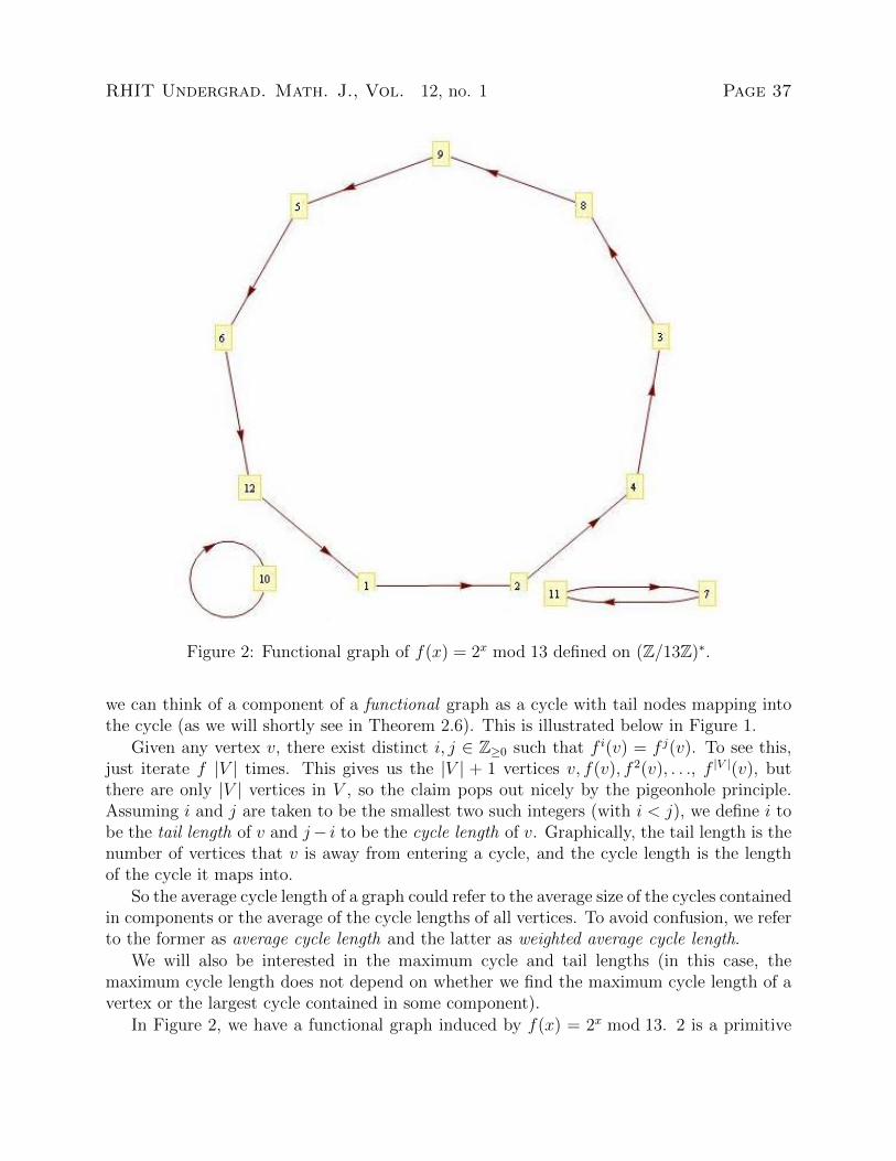
Figure 2: Functional graph of f(x) = 2x mod 13 defined on (Z/13Z)∗.
we can think of a component of a functional graph as a cycle with tail nodes mapping intothe cycle (as we will shortly see in Theorem 2.6). This is illustrated below in Figure 1.
Given any vertex v, there exist distinct i, j ∈ Z≥0 such that f i(v) = f j(v). To see this,just iterate f |V | times. This gives us the |V | + 1 vertices v, f(v), f 2(v), . . ., f |V |(v), butthere are only |V | vertices in V , so the claim pops out nicely by the pigeonhole principle.Assuming i and j are taken to be the smallest two such integers (with i < j), we define i tobe the tail length of v and j− i to be the cycle length of v. Graphically, the tail length is thenumber of vertices that v is away from entering a cycle, and the cycle length is the lengthof the cycle it maps into.
So the average cycle length of a graph could refer to the average size of the cycles containedin components or the average of the cycle lengths of all vertices. To avoid confusion, we referto the former as average cycle length and the latter as weighted average cycle length.
We will also be interested in the maximum cycle and tail lengths (in this case, themaximum cycle length does not depend on whether we find the maximum cycle length of avertex or the largest cycle contained in some component).
In Figure 2, we have a functional graph induced by f(x) = 2x mod 13. 2 is a primitive
Page 38 RHIT Undergrad. Math. J., Vol. 12, no. 1
root modulo 13, so this is a permutation. Every vertex is therefore cyclic, so the tail lengthof every vertex is 0. Vertex 10 has cycle length 1, vertices 7 and 11 have cycle length 2,and so on. There are 3 components (and cycles), the average cycle length is 4, and theweighted average cycle length is 86
12≈ 7.17. This example shows that average cycle length
and weighted average cycle length encode different information about a graph.
We will need a couple of general results about functional graphs later in the paper, thefirst of which appears in the paper by Flajolet and Odlyzko [4]. We state them here.
Theorem 2.6. If f : V → V is a function with V finite, and G = (V,E) is the inducedfunctional graph, then every component of G has exactly one cycle.
Theorem 2.7. If G = (V,E) is a binary functional graph with n vertices, then G has exactlyn/2 terminal nodes and n/2 image nodes.
Proof. The Handshaking Theorem [8, p. 548] tells us that∑
v∈V deg−(v) = |E|. Since thereis one edge for every vertex, this is equal to n. The fact that each image node has exactlytwo preimages in a binary functional graph (and there can be no overlap since deg+(v) = 1for all v ∈ V ) implies that the number of image nodes is n/2, which also implies that thereare n/2 terminal nodes.
This can, in fact, be generalized to show that for an m-ary functional graph of order n,there are (m − 1)n/m terminal nodes and n/m image nodes. We can also conclude thatthe number of vertices in every component of an m-ary functional graph is divisible by mby observing that (after including the necessary edges) a component of an m-ary functionalgraph is an m-ary functional graph in its own right.
2.3 Random Functional Graphs
The whole reason for appealing to functional graphs is that graph theory is well studied,whereas discrete logs are somewhat mysterious by comparison. The goal is to create a mapbased on elliptic curve discrete exponentiation, from which we can create a functional graphin order to identify any noticeable patterns. These could lead us to attacks against discretelogs on elliptic curves, or convince us that such maps are indeed random.
Random functional graphs (where we consider the graph induced by each function f :V → V to be likely to occur with equal probability) have been fairly thoroughly studied. Fla-jolet and Odlyzko, for example, provide an analysis in [4]. They use exponential generatingfunctions and give expected asymptotic values of various statistics for a random functionalgraph with n vertices. Similar results regarding binary functional graphs with n verticesappear in Cloutier and Holden’s paper [3]. We summarize the results below.
Random Functional Graphs:

RHIT Undergrad. Math. J., Vol. 12, no. 1 Page 39
Statistic Expected Asymptotic Value
Number of Components1
2(log (2n) + γ)
Number of Cyclic Nodes√πn/2− 1
3
Number of Tail Nodes n−√πn/2 +
1
3Number of Terminal Nodes e−1nNumber of Image Nodes (1− e−1)nNumber of k-cycles 1/k
Average Cycle Length
√πn/2− 1
32(log (2n) + γ)
Weighted Average Cycle Length√πn/8
Average Tail Length√πn/8
Maximum Cycle Length c
√πn
2≈ 0.78248
√n
Maximum Tail Length√
2πn log 2 ≈ 1.73746√n
Random Binary Functional Graphs:
Statistic Expected Asymptotic Value
Number of Components1
2(log (2n) + γ)
Number of Cyclic Nodes√πn/2− 1
Number of Tail Nodes n−√πn/2 + 1
Number of Terminal Nodes n/2Number of Image Nodes n/2
Average Cycle Length
√πn/2− 1
2(log (2n) + γ)Weighted Average Cycle Length
√πn/8
Average Tail Length√πn/8
Maximum Cycle Length c
√πn
2≈ 0.78248
√n
Maximum Tail Length√
2πn log 2− 3 + 2 log 2 ≈ 1.73746√n− 1.61371
Here c refers to the constant∫ ∞0
(1− exp
(−∫ ∞v
e−u du
u
))dv.
It should be noted that cyclic and tail nodes are dual to each other, as are terminal and imagenodes (i.e., knowledge of one is equivalent to knowledge of the other). Also, the average cyclelength is the ratio of cyclic nodes to the number of components. The other observation to

Page 40 RHIT Undergrad. Math. J., Vol. 12, no. 1
make is that these are expected asymptotic values, which means we should compare dataagainst these theoretical values when n is fairly large.
We now show that the expected number of k-cycles for a random binary functional graphis 1/k, just as in the more general case. This result does not seem to appear in the literature,but the proof is very similar to those found in the papers by Cloutier [2] and by Flajolet andOdlyzko [4].
Theorem 2.8. The expected number of k-cycles for a random binary functional graph is1/k.
Proof. We first enumerate binary functional graphs combinatorially so that they can beconverted into exponential generating functions. This is done as follows [4].
BinFunGraph = set(Component);
Component = cycle(BinTree);
BinTree = Node * set(BinTree);
Node = Atomic Unit.
In other words, a binary functional graph is a set of components; a component is a cycleof binary trees; a binary tree is a node attached to a set of zero or two (possibly empty)binary trees; a node is an atomic unit.
In general, given a class of combinatorial objects C, if we let Cn denote those of sizen, there is a certain power series known as an exponential generating function C(z) =∑
n≥0Cnzn
n![4]. Therefore, we can obtain exponential generating functions for binary func-
tional graphs, components, binary trees, and nodes. The exponential generating functionsfor binary functional graphs, components, and binary trees are denoted f(z), c(z), and b(z),respectively. These functions, as described in Cloutier’s paper [2], are given below.
f(z) =1√
1− 2z2,
c(z) = log1√
1− 2z2,
b(z) = z +1
2zb2(z).
Now the closed-form expression for b(z) is
b(z) =1−√
1− 2z2
z.
The proof for the case of random functional graphs from Flajolet and Odlyzko’s paper [4]uses a bivariate exponential generating function with the variable u marking k-cycles. Thisfunction is based on the formulas for f(z), c(z), and b(z). We imitate the proof by using

RHIT Undergrad. Math. J., Vol. 12, no. 1 Page 41
the formulas for binary functional graphs, as described above. The bivariate exponentialgenerating function is the following.
g(u, z) = exp
(log
(1
1− 2z2
)+ (u− 1)
(zb(z))k
k
).
Proceeding as in Flajolet and Odlyzko’s paper [4], we compute gu(1, z) =zkb(z)k
k√
1− 2z2. Sin-
gularity analysis using the Maple package Algolib reveals that the asymptotic behavior ofthe nth coefficient of this expression is
21/2+n/2
√1
n+O
(2n/2
n3/2
)√πk
√πk
.
Now this represents the number of k-cycles in all binary functional graphs with n vertices.We must normalize this, therefore, by dividing by the number of binary functional graphswith n vertices, which can be shown to be n!
(nn/2
)/2n/2 [7], and multiplying by n! since in
an exponential generating function for the sequence (an), each term is of the form ann!xn.
Asymptotic analysis in Maple shows that the resulting expression is asymptotic to
1
k+O
(1
n
),
and the term that interests us falls out nicely as1
k.
3 Prior Work
Daniel Cloutier [2], Nathan Lindle [7] and Andrew Hoffman [5] have worked on investigatingthe classical discrete logarithm problem by investigating related functional graphs. Theirmethods involved computing the number of components, sizes of cycles, numbers of tailand cyclic nodes, and so on, on thousands of functional graphs. They used exponentialgenerating functions to calculate the expected values of random functional graphs, as wellas particular classes of random functional graphs (e.g., random permutations and binaryfunctional graphs). Cloutier chose to look at permutations and binary functional graphsin particular because the data he collected was quite inconsistent with random functionalgraphs, but in many cases turned out to be very accurate compared to the theoretical valuesfor random permutations and binary functional graphs.
No previous work has been done on functional graphs associated with discrete logs onelliptic curves. Given an elliptic curve E(Fp) with N points, the author’s goal has been toinvestigate them by the map
k 7→ x(kB) for k ∈ {0, 1, . . . , N − 1} , ∞ 7→ ∞.
Page 42 RHIT Undergrad. Math. J., Vol. 12, no. 1
It turns out these graphs are binary, so the author followed suit in heavy computation inorder to compare the data to what would be expected of random binary functional graphs.
Ultimately, we would like to be assured that discrete exponentiation actually behaves likea random map for security reasons. If there is some way to exploit any structure it imposes,however, we would like to know what it is so that we can either abandon relying on thediscrete log problem if it is breakable (which seems unlikely) or perhaps ensure that certainconditions are satisfied so that we can continue to communicate with one another securely(for example, in the classical discrete log problem, it is common practice to make sure thatp− 1 has a large prime factor).
4 Elliptic Curve Functional Graphs
It is relatively straightforward to devise a function to induce a functional graph that describesdiscrete exponentiation in the classical case. Simply map x 7→ gx mod p for some nonzerog. With elliptic curves, however, the situation is rather subtle. Our “exponent” (i.e., thenumber k in the equation kB = P ) is an integer, but our points are not, and we would liketo take an integer k and consider kB. Two possibilities are the following:
• P 7→ x(P )B
• k 7→ x(kB)
In both cases, x(P ) denotes the x-coordinate of the point P , B is a generator, and wealso map ∞ 7→ ∞.
In Appendix A, we show that the first map never induces a binary functional graph.Therefore, the map P 7→ x(P )B is not as interesting to study. However, we will shortly seethat the map k 7→ x(kB) gives us binary functional graphs as long as N = #E(Fp) ≥ p isodd. Therefore, we investigate the map k 7→ x(kB),∞ 7→ ∞. We shall refer to these graphsas ECFGs (elliptic curve functional graphs) from now on.
We illustrate with an example in Figure 3.
4.1 Theoretical Results
We state one of the most important theoretical results about ECFGs in the next theorem.First, however, we require a lemma.
Lemma 4.1. If E(Fp) is cyclic of order N (with N odd), then x3 + ax + b ≡ 0 (mod p) isinsoluble.
Proof. The order of E(Fp) is p+ 1 +∑p−1
x=0
(x3+ax+b
p
). Since N and p are odd, the Legendre
sum must also be odd. Therefore, it suffices to show that∑p−1
x=0
(x3+ax+b
p
)has no 0 terms in
the sum. Since Fp is a field and the polynomial x3 + ax + b has degree 3, there must be at

RHIT Undergrad. Math. J., Vol. 12, no. 1 Page 43
Figure 3: ECFG of E(F17) : y2 = x3 + x+ 3 with generator B = (2, 8) (this curve has orderN = p = 17).
Page 44 RHIT Undergrad. Math. J., Vol. 12, no. 1
most 3 zeros. If there are no zeros, there is nothing to prove. Suppose we have one or three0 terms in the sum. Then since p− 1 and p− 3 are even, a sum of p− 1 or p− 3 odd termsmust be even, so the sum cannot be odd in this case. Now suppose x3 + ax + b has 2 zerosin Fp. Put x3 + ax + b = (x − α)(x − β)g(x). But then g(x) must be of degree one, whichforces f(x) to have a third zero, a contradiction.
Proof. Here is an alternative proof. Let x0 ∈ Fp such that x30 + ax0 + b ≡ 0 (mod p). Thenthe point P = (x0, 0) lies on E. Therefore 2P = ∞. So P generates a subgroup of E oforder 2. By Lagrange’s theorem, N must be even.
Now we are ready to prove our theorem.
Theorem 4.2. Let E(Fp) be cyclic of order N (N ≥ p odd). Let B be a generator, andG = (V,E) be the induced ECFG. Then G is binary, and k and −k map to the same vertexfor all k ∈ Z/NZ.
Proof. Let x0 6= ∞ ∈ V . If deg−(x0) = 0, then there is nothing to prove. If deg−(x0) ≥ 1,then there is a k ∈ Z/NZ with kB = (x0, y0), so (N − k)B = −kB = (x0,−y0). This meansthat both k and −k map to x0. These points are distinct as long as y0 6≡ 0 (mod p), whichholds by Lemma 4.1. Now if there is a third integer r with rB = (x0, y1), then we musthave rB 6= ±kB since N ≥ p because after computing a multiple of a generator, we reducethe coordinates modulo p, then the exponent modulo N . Thus, kB,−kB, and rB are alldistinct, so they lie on the vertical line x = x0. This means that kB + −kB + rB = ∞,which forces rB = ∞. Therefore, rB is not a finite point. So we have shown the result forall finite points.
Now for x0 =∞, by construction, we have x0 7→ x0. Furthermore, we have 0 7→ x0 since0B = ∞. Now suppose there is a third preimage l — i.e., x(lB) = ∞. This means thatlB =∞, which means that l ≡ 0 (mod N), but l must belong to Z/NZ, so we actually havel = 0. Therefore, ∞ cannot have a third preimage.
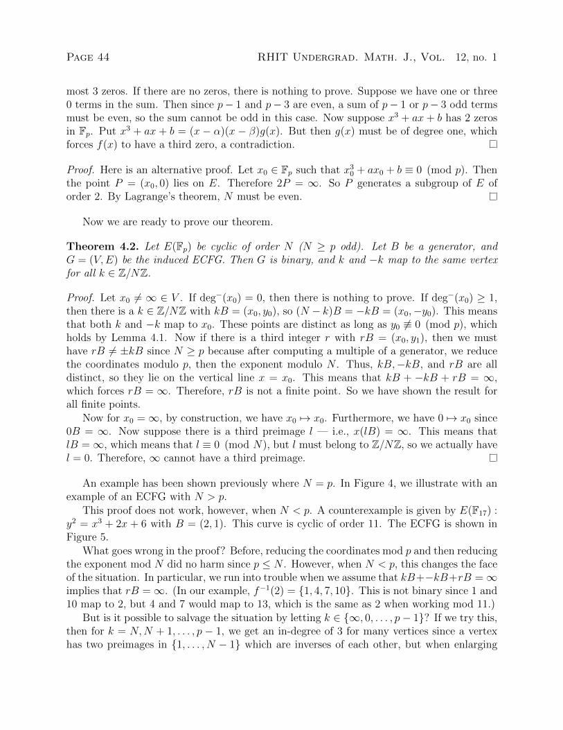
An example has been shown previously where N = p. In Figure 4, we illustrate with anexample of an ECFG with N > p.
This proof does not work, however, when N < p. A counterexample is given by E(F17) :y2 = x3 + 2x + 6 with B = (2, 1). This curve is cyclic of order 11. The ECFG is shown inFigure 5.
What goes wrong in the proof? Before, reducing the coordinates mod p and then reducingthe exponent mod N did no harm since p ≤ N . However, when N < p, this changes the faceof the situation. In particular, we run into trouble when we assume that kB+−kB+rB =∞implies that rB =∞. (In our example, f−1(2) = {1, 4, 7, 10}. This is not binary since 1 and10 map to 2, but 4 and 7 would map to 13, which is the same as 2 when working mod 11.)
But is it possible to salvage the situation by letting k ∈ {∞, 0, . . . , p− 1}? If we try this,then for k = N,N + 1, . . . , p − 1, we get an in-degree of 3 for many vertices since a vertexhas two preimages in {1, . . . , N − 1} which are inverses of each other, but when enlarging
RHIT Undergrad. Math. J., Vol. 12, no. 1 Page 45
Figure 4: ECFG of E(F23) : y2 = x3 + x+ 4 with generator B = (7, 3) (this curve has orderN = 29 > p).

Page 46 RHIT Undergrad. Math. J., Vol. 12, no. 1
Figure 5: ECFG of E(F17) : y2 = x3 + 2x+ 6 with generator B = (2, 1) (this curve has orderN = 11 < p).
RHIT Undergrad. Math. J., Vol. 12, no. 1 Page 47
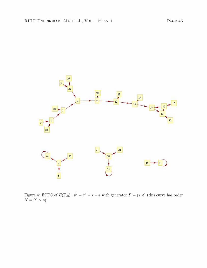
Figure 6: ECFG of E(F17) : y2 = x3+2x+6 with generator B = (2, 1) with domain extendedto Z/pZ ∪ {∞} (this curve has order N = 11 < p).
Page 48 RHIT Undergrad. Math. J., Vol. 12, no. 1
the domain and computing kB, we reduce k mod N . N is often large enough to get a thirdpreimage for v. Let us make things concrete and display the functional graph in Figure 6.
In our example, 13 gets mapped to by 4 and 7, but when extending our domain, it alsogets mapped to by 15. The next number congruent to 7 (mod 11), however, is 18, whichis too large. As in the previous paragraph, we go wrong in this function definition whenassuming kB + −kB + rB = ∞ implies that rB = ∞ since here rB = ±kB (i.e., r ≡ ±k(mod N)). The problem here is that r ≡ ±k (mod N) does not imply that r = ±k.
Therefore, in this paper, we consider elliptic curves over Fp of order N ≥ p (which isnot to suggest that there is no interest in looking at curves of smaller order, but differenttechniques must then be applied since they will not result in binary functional graphs).
Proposition 4.3. If(bp
)= −1, then G has a component {0,∞}. If
(bp
)= 1, then ∞ is
part of a larger component.
Proof.(bp
)= −1 means that (0, y) cannot lie on the elliptic curve E(Fp) for any y ∈ Fp.
Therefore, there is no k ∈ Z/NZ with k 7→ 0. But it is apparent that 0 7→ ∞ 7→ ∞.
If(bp
)= 1, however, then (0, y) does lie on E(Fp) for some y ∈ Fp, and since E(Fp) is
generated by a point B, there is some k ∈ Z/nZ such that kB = (0, y). Thus, k 7→ 0 7→∞ 7→ ∞.
What happens if(bp
)= 0? This means b ≡ 0 (mod p), or that E is described by
y2 = x3 + ax. If a = 0, then this is not an elliptic curve; otherwise, we have the following.
Theorem 4.4. If E is an elliptic curve over Fp with N points and b = 0, then N is even.
Proof. Suppose that b = 0. Then the order of E(Fp) is p + 1 +∑p−1
x=0
(x3+axp
). This sum is
even if and only if the sum∑p−1
x=1
(x3+axp
)is even (notice that
(03+a·0p
)contributes nothing
to this sum).Since p ≥ 5, p ≡ 1 or 3 (mod 4). So there are two cases. Notice that x3 + ax is an odd
function. The idea is to pair up the additive inverses in the Legendre symbols.
Case 1 : If p ≡ 1 (mod 4), then(αp
)+(−αp
)= 2
(αp
), so when pairing up and adding
the Legendre symbols for each pair of additive inverses, the resulting sum is even. Therefore,
the sum∑p−1
x=1
(x3+axp
)is even.
Case 2 : If p ≡ 3 (mod 4), then(αp
)+(−αp
)= 0, so when pairing up and adding
the Legendre symbols for each pair of additive inverses, the resulting sum is equal to 0.
Therefore,∑p−1
x=1
(x3+axp
)= 0.
We have shown that the sump−1∑x=1
(x3 + ax
p
)is always even, which yields the result.
RHIT Undergrad. Math. J., Vol. 12, no. 1 Page 49
Proof. Here is an alternative proof. Suppose E(Fp) : y2 = x3 + ax is an elliptic curve. ThenP = (0, 0) ∈ E, and 2P = ∞, so we have a subgroup of order 2, which, by Lagrange’stheorem, implies that N is even.
Remark. In cryptographic settings, it is typical to ensure that #E(Fp) = q, where q isa prime (not necessarily q = p). Thus, the importance of this result may become clearerwhen stated in the contrapositive: if #E(Fp) = N is odd (perhaps even prime), then b 6≡ 0(mod p), so we know there are exactly two cases for what sort of component ∞ can lie in.So while it is still of theoretical interest to consider curves of even order, we ignore the caseb ≡ 0 (mod p) in this paper.
One other thing to count on these graphs is the number of terminal (or equivalently,image) nodes. The reason for the in-degree being 0 could be that for a particular x0, x
30 +
ax0 + b is not a square in Fp, that the base point B does not map to this value in thisfunctional graph, or that x > p− 1 since we always reduce the coordinates modp. However,the fact that B is a generator eliminates the second possibility.
It turns out that for N ≥ p odd, there are (N + 1)/2 terminal nodes, and therefore(N + 1)/2 image nodes. We prove this result first when the order of the curve is exactly p,then for the case where N > p. Note that the following proposition is equivalent to statingthat when N = p, the ECFG of E has exactly (p+ 1)/2 terminal nodes (and therefore also(p+ 1)/2 image nodes).
Proposition 4.5. If x3 + ax+ b defines a cyclic elliptic curve E(Fp) of order p, then there
are exactly p+12
values of x ∈ Fp such that(x3+ax+b
p
)= −1.
Proof. Since p is odd, we know that x3 + ax + b ≡ 0 (mod p) has no solution by Lemma
4.1. We also know that∑p−1
x=0
(x3+ax+b
p
)= −1. Therefore, each term in the sum contributes
±1 to the sum. There are p terms in the sum and we need one more -1 than 1s in the sum.Let s count the number of 1s. Then s+ 1 counts the number of -1s. This gives the equation2s+ 1 = p, which means that s = (p− 1)/2. Therefore, s+ 1 = (p+ 1)/2.
Now we prove the result for N > p in the following theorem.
Theorem 4.6. If N > p is odd, there are always (N + 1)/2 terminal nodes (and therefore(N + 1)/2 image nodes).
Proof. We know that N = p + 1 +∑p−1
x=0
(x3+ax+b
p
). Since N > p is odd, it follows that
N = p+r for some r in Z≥2. This means p+1+∑p−1
x=0
(x3+ax+b
p
)= p+r, or
∑p−1x=0
(x3+ax+b
p
)=
r − 1. We know that x3 + ax + b = 0 is unsolvable in Fp by Lemma 4.1 (so there are only
±1s in the Legendre sum) and that∑p−1
x=0
(x3+ax+b
p
)is positive. Therefore, there are at least
r− 1 1s in the Legendre sum, so we choose r− 1 (which is odd since N and p are odd, whichmeans that r must be even) squares in Fp, and let s count the number of -1s. Therefore,

Page 50 RHIT Undergrad. Math. J., Vol. 12, no. 1
s + (r − 1) counts the number of 1s. Then s + (s + (r − 1)) = 2s + (r − 1) = p. This givess = (p− (r−1))/2. By the discussion preceding Proposition 4.5, we need to add the numberof integers modulo N greater than p − 1 to s to count the number of terminal nodes. Thisnumber is (N − 1)− (p− 1) = N − p. So the following computation yields the result.
s+ (N − p) = (p− (r − 1))/2 + 2(N − p)/2= (p− (r − 1) + 2(N − p))/2= (p− (r − 1) + 2r)/2
= (p+ r + 1)/2
= (N + 1)/2.
In fact, we can prove this more generally for any binary functional graph. See Theorem2.7 for the details.
One question of theoretical interest is the following: can we also look at functional graphsof proper subgroups of a given elliptic curve? The answer is a resounding no.
We know we want to look at curves with N ≥ p, but if we want a subgroup, we want aproper divisor r of N such that r ≥ p. However, Hasse’s Theorem tells us that an ellipticcurve over Fp has N ≤ p+ 1 + 2
√p points [9, p. 97]. Suppose that r | N,N > r ≥ p. Then
N ≥ 2r ≥ 2p. But for p > 5,
√p− 2 >
1√p
√p(√p− 2) = p− 2
√p > 1
p > 1 + 2√p
2p > p+ 1 + 2√p ≥ N
N ≥ 2r ≥ 2p > N.
This shows that considering such subgroups is fruitless.
4.2 Computational Results
One fact is that B and −B generate the same group. But they also induce the same ECFG.This can be seen as follows: kB = (x, y) if and only if k(−B) = −kB = (x,−y), so k 7→ xin the graph with generator B if and only if −k 7→ x in the graph with generator −B. ByTheorem 4.2, in both graphs, k 7→ x and −k 7→ x for all x 6=∞. The only preimages of ∞are 0 and ∞ regardless of the generator (in fact, regardless of the curve). This fact allowsus to analyze only half as many graphs as we would otherwise have to.
There is another theoretical idea we can use to speed up computation. The largestpossible cycle is of size N − 1 since there is always a fixed point at ∞ and we also have

RHIT Undergrad. Math. J., Vol. 12, no. 1 Page 51
0 7→ ∞. By Theorem 2.6, every component in a functional graph contains exactly one cycle,so the number of cycles is equal to the number of components. Therefore, if Ci denotesthe number of i-cycles, and r denotes the number of components, then
∑N−1i=1 Ci = r. It is
much quicker to use a cycle-finding algorithm to compute the number of cycles than it isto construct a graph and use an algorithm such as depth-first search to partition the graphinto its components.
In order to gather statistics, the author wrote three computer programs. The first is aJava program that takes in a prime N and finds all elliptic curves of order N over fields Fpwith p ≤ N . This uses an array of prime numbers, the bounds on N implied by Hasse’sTheorem, and a simple search (for each curve, it also finds the generators for the curve byiterating over Fp and computing square roots). It then outputs the values of a, b, p and B(the generator) to a file for each curve-generator pair. The second program, written in C,reads in this file, and for each curve-generator pair, computes the number of terminal nodes,image nodes, fixed points, two-cycles, three-cycles, five-cycles, components (or equivalently,cycles), cyclic nodes, tail nodes, as well as the average cycle length, weighted average cyclelength, average tail length, the maximum cycle length, and the maximum tail length. Thesecomputations are performed by using Brent’s algorithm for finding cycles in iterated functionsand by computing Jacobi symbols (a slightly faster method of computing Legendre symbols).These statistics for each ECFG are then output to a file.
The third program is a Java program that reads in the file output from the secondprogram and for each statistic, prints out the expected value, mean and variation for eachstatistic (this is all within a particular prime N).
One problem with gathering statistics for all ECFGs of some fixed order N is that thereis an astronomical number of graphs to create. With the classical discrete log problem, thereare p−1 different graphs (and only ϕ
(p−12
)different binary graphs). However, in the ECFG
case, for a fixed N , p varies when finding the prime fields Fp, and for each prime field, thereseem to be on the order of N different elliptic curves. Furthermore, for each elliptic curve,there are ϕ(N) graphs to create (which, when N is prime, is equal to N−1). Even at a quitesmall value of N = 83, there are already 34,112 graphs. For N = 211, there are 549,780graphs. We know that a given curve with generators B and −B induce the same ECFG, sothis cuts down on the computation we have to do drastically, but unless we can find deeperresults about when various generators induce isomorphic ECFGs, it seems highly unlikelythat we can record very many asymptotic statistics for these graphs. In any case, someresults are tabulated below.

Page 52 RHIT Undergrad. Math. J., Vol. 12, no. 1
N = 167 (208,496 graphs)Statistic Expected Observed VarianceTerminal Nodes 84 84 0Image Nodes 84 84 0Fixed Points 1 1.992422 0.9767862-cycles 0.5 0.475012 0.4758743-cycles 0.3̄ 0.318932 0.3124305-cycles 0.2 0.182804 0.177953Components 3.197163 4.085517 1.972782Average Cycle Length 4.768229 3.852527 4.191673Cyclic Nodes 15.244808 15.126151 57.433792Tail Nodes 152.755192 152.873849 57.433792Weighted Average Cycle Length 8.122404 7.014287 25.312406Average Tail Length 8.122404 7.125777 9.990484Max Cycle Length 10.142100 9.076117 31.394953Max Tail Length 24.133765 18.032260 34.678483
N = 211 (549,780 graphs)Statistic Expected Observed VarianceTerminal Nodes 106 106 0Image Nodes 106 106 0Fixed Points 1 1.994940 0.9768052-cycles 0.5 0.502165 0.4939473-cycles 0.3̄ 0.316221 0.3155965-cycles 0.2 0.189228 0.185972Components 3.313475 4.238230 2.122886Average Cycle Length 5.205572 4.279185 5.455133Cyclic Nodes 17.248529 17.339449 74.948891Tail Nodes 194.751471 194.660551 74.948891Weighted Average Cycle Length 9.124265 8.161955 33.787259Average Tail Length 9.124265 8.109176 13.359563Max Cycle Length 11.393081 10.445054 41.073544Max Tail Length 26.911509 20.660497 46.404844

RHIT Undergrad. Math. J., Vol. 12, no. 1 Page 53
N = 227 (292,896 graphs)Statistic Expected Observed VarianceTerminal Nodes 114 114 0Image Nodes 114 114 0Fixed Points 1 1.996238 1.0129672-cycles 0.5 0.501106 0.5037133-cycles 0.3̄ 0.340052 0.3405675-cycles 0.2 0.176861 0.171720Components 3.349854 4.303398 2.220580Average Cycle Length 5.350868 4.449070 5.928930Cyclic Nodes 17.924628 18.176977 80.148224Tail Nodes 210.075372 209.823023 80.148224Weighted Average Cycle Length 9.462314 8.647097 38.137383Average Tail Length 9.462314 8.453528 14.086671Max Cycle Length 11.815189 10.967579 45.399227Max Tail Length 27.848781 21.570455 48.971410
Although we cannot compute these statistics over all ECFGs for N large, we can try topick a random selection of ECFGs for larger values of N and see how the limited statisticsmatch up to the expected values. The author modified the program to find elliptic curvesof a given order to find randomly chosen curve-generator pairs. Displayed below are limitedstatistics for somewhat larger primes.
N = 419 (100,000 graphs)Statistic Expected Observed VarianceTerminal Nodes 210 210 0Image Nodes 210 210 0Fixed Points 1 1.994600 0.9950912-cycles 0.5 0.493040 0.4942723-cycles 0.3̄ 0.331530 0.3285785-cycles 0.2 0.193690 0.190394Components 3.655309 4.601670 2.433203Average Cycle Length 6.753273 5.718504 10.352899Cyclic Nodes 24.685297 24.939260 157.386731Tail Nodes 395.314703 395.060740 157.386731Weighted Average Cycle Length 12.842648 12.055864 75.266458Average Tail Length 12.842648 11.880105 28.272666Max Cycle Length 16.036068 15.247660 89.399045Max Tail Length 37.221044 30.789860 98.998861
Page 54 RHIT Undergrad. Math. J., Vol. 12, no. 1
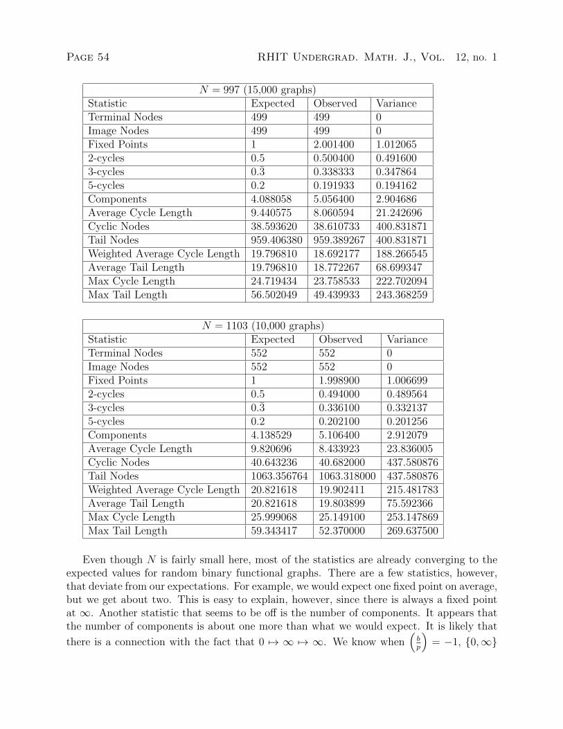
N = 997 (15,000 graphs)Statistic Expected Observed VarianceTerminal Nodes 499 499 0Image Nodes 499 499 0Fixed Points 1 2.001400 1.0120652-cycles 0.5 0.500400 0.4916003-cycles 0.3̄ 0.338333 0.3478645-cycles 0.2 0.191933 0.194162Components 4.088058 5.056400 2.904686Average Cycle Length 9.440575 8.060594 21.242696Cyclic Nodes 38.593620 38.610733 400.831871Tail Nodes 959.406380 959.389267 400.831871Weighted Average Cycle Length 19.796810 18.692177 188.266545Average Tail Length 19.796810 18.772267 68.699347Max Cycle Length 24.719434 23.758533 222.702094Max Tail Length 56.502049 49.439933 243.368259
N = 1103 (10,000 graphs)Statistic Expected Observed VarianceTerminal Nodes 552 552 0Image Nodes 552 552 0Fixed Points 1 1.998900 1.0066992-cycles 0.5 0.494000 0.4895643-cycles 0.3̄ 0.336100 0.3321375-cycles 0.2 0.202100 0.201256Components 4.138529 5.106400 2.912079Average Cycle Length 9.820696 8.433923 23.836005Cyclic Nodes 40.643236 40.682000 437.580876Tail Nodes 1063.356764 1063.318000 437.580876Weighted Average Cycle Length 20.821618 19.902411 215.481783Average Tail Length 20.821618 19.803899 75.592366Max Cycle Length 25.999068 25.149100 253.147869Max Tail Length 59.343417 52.370000 269.637500
Even though N is fairly small here, most of the statistics are already converging to theexpected values for random binary functional graphs. There are a few statistics, however,that deviate from our expectations. For example, we would expect one fixed point on average,but we get about two. This is easy to explain, however, since there is always a fixed pointat ∞. Another statistic that seems to be off is the number of components. It appears thatthe number of components is about one more than what we would expect. It is likely that
there is a connection with the fact that 0 7→ ∞ 7→ ∞. We know when(bp
)= −1, {0,∞}
RHIT Undergrad. Math. J., Vol. 12, no. 1 Page 55
is its own component. This happens with probability about 1/2. But even if b is a squaremod p, each of 0’s two preimages has a probability of about 1/2 (actually, N/2p) of having apreimage. In other words, if r 7→ 0, then r has a preimage only if r3 + ra+ b is a square modp. To go backwards i iterations, the probability of the preimage being nonempty is about(N2p
)i≈ 1
2i. Therefore, it is quite likely that the component containing ∞ is fairly small.
This suggests that there should be about one more component than we would expect froma random binary functional graph.
The other three statistics that seem off are average cycle length, maximum cycle lengthand maximum tail length. Average cycle length tends to be off by about 0.9. However, sincethe average cycle length can be computed by cyclic nodes / components, this deviation isequivalent to the number of components deviating (notice that the number of cyclic nodesmatches up quite accurately compared to the expected value).
One possible explanation of why the maximum cycle length is off is because of the fixedpoint at ∞. If we consider the binary functional graph by removing ∞’s component, we geta binary graph with fewer vertices, and the maximum cycle length might match up betterto the expected value for this subgraph. An explanation of why the maximum tail length isoff seems more elusive, however. It is consistently under the expected value by about 6 or 7.This suggests that discrete exponentiation on elliptic curves is slightly less secure than onemight hope for two reasons. First, it suggests that there’s less of a chance for a longer tail,which could prove detrimental for certain pseudorandom number generators [1]. Secondly,it seems to suggest that there is some extra structure in the maps we’ve been considering,which could lead to an attack on the discrete logarithm problem.
5 Conclusions and Future Work
The hardness of the discrete logarithm problem on elliptic curves has offered an advance incryptography, and there is computational evidence that suggests that it is even more securethan classical techniques. It is assumed to be secure because of the belief that discreteexponentiation behaves like a random map. If, however, there is some structure imposed bydiscrete exponentiation for elliptic curves, we want to know the details so that we can eitherabandon relying on the discrete logarithm problem or else ensure that certain conditions aremet so that the discrete logarithm problem remains hard.
Most of the statistics collected for ECFGs do match up with what would be expectedof a random map. There are, however, a couple of areas where there does seem to besome extra structure imposed by discrete exponentiation. One area is the maximum taillength. This seems to be consistently lower than the expected theoretical value of a randombinary map by about 6 or 7. The deviation seems too extreme to be caused just by the smallcomponent containing∞. Indeed, Lindle [7] seemed to be stuck with the same anomaly wheninvestigating binary functional graphs in the discrete logarithm problem modulo p. Perhapsthis information could be used to devise an attack on the discrete logarithm problem.
More significantly, however, most of the other deviations in the statistics seem to be
Page 56 RHIT Undergrad. Math. J., Vol. 12, no. 1
caused by the small component containing the cycle at infinity. In addition to applicationsof the hardness of the discrete logarithm problem on elliptic curves to Diffie-Hellman andElGamal, there are also random number generators that exploit the discrete log’s hardness.For example, in [1], a map is specified by k 7→ t(x(kB)), where t(x) processes the x-coordinatein some way. One thing that we want to ensure when using this random number generatoris that we don’t quickly enter a short cycle. Although for a curve with a large number ofpoints, it is relatively unlikely that an initial seed k belongs to a small component, it canhappen. If it does, then the random number generator will no longer be secure. One smallcomponent in particular is the one containing ∞. We can iterate our map to see if we geta fixed point (which would give rise to an eventually constant sequence). This weaknessdoesn’t seem to be as exploitable in Diffie-Hellman, however, because knowing that thereis an incoming edge to x0, where P = (x0, y0) (we can also figure this out by computing aLegendre symbol) doesn’t seem to give us extra information about how to solve the discretelogarithm kB = P .
There are a number of ways in which this project can be continued. One quite spe-cific continuation is investigating why the maximum cycle and tail length deviate from ourexpectation, particularly maximum tail length.
Another way to continue this project would be simply to collect more data and performmore thorough statistical analyses. Yet another idea would be to investigate curves of orderN < p, which I have chosen to neglect since these curves do not induce binary functionalgraphs. Similarly, curves of even order could be investigated, perhaps even supersingularcurves. Other related functions such as P 7→ x(P )B could also be considered (these do notinduce binary functional graphs).
I have also chosen to ignore elliptic curves over non-prime fields Fq. One reason forignoring other curves is that it is simpler to implement the arithmetic in the prime case. Ihave also ignored curves over F2 and F3. There is not a huge number of curves over thesefields, so this is not a huge limitation; however, elliptic curves over F2k in particular might beworth investigating since these binary fields are often used in cryptography (and arithmeticover F2k would be easier to implement than arithmetic in Fpk for arbitrary p).
A The Map P 7→ x(P )B
In this appendix, we prove a couple of properties of the map mentioned earlier in this paper:P 7→ x(P )B,∞ 7→ ∞, where P is a point on an elliptic curve E(Fp), B is a generator, andx(P ) denotes the x-coordinate of the point P .
Proposition A.1. Let E(Fp) : y2 = x3 + ax + b be an elliptic curve with N points. ThenP 7→ x(P )B does not induce a binary functional graph (regardless of the generator B).
Proof. If we have an odd number of points on the curve, then the graph cannot be binaryby the remarks that follow Theorem 2.7.
If we have an even number of points, then since E(Fp) is abelian, there is a subgroup oforder 2, and the generator of this subgroup has to have y−coordinate equal to 0. Let this
RHIT Undergrad. Math. J., Vol. 12, no. 1 Page 57
generator be denoted by Q = (x, 0). Now let P = x(Q)B = xB. If there were a secondpreimage, then we would have P = x(R)B, and thus x(R) = x(Q). But there can only beone point on the curve with x-coordinate x(Q) since Q = −Q.
Therefore, the map P 7→ x(P )B never induces a binary functional graph.
Remark. Many of the vertices in these graphs do have two preimages, however (and ∞can have three preimages in some cases). Therefore, these do not produce m-ary functionalgraphs for any m.
Proposition A.2. {∞} is its own component if and only if(bp
)= −1.
Proof. Once we have specified our generator B, we can identify any point on the curveuniquely by an integer modulo N . Thus, ∞ has a preimage if and only if we can solve
0 = x(P ) for some P ∈ E, which is solvable if and only if(bp
)= 1.
References
[1] Brown, Daniel R. L. and Gjøsteen, Kristian, A Security Analysis of the NIST SP800-90 Elliptic Curve Random Number Generator. In CRYPTO 2007, LNCS 4622,pages 466-481. 2007.
[2] Cloutier, Daniel. R., Mapping the Discrete Logarithm. Senior thesis, Rose-HulmanInstitute of Technology, 2005.
[3] Cloutier, Daniel R. and Holden, Joshua, Mapping the Discrete Logarithm. 2006.http://xxx.lanl.gov/abs/math.NT/0605024
[4] P. Flajolet and A. Odlyzko, Random Mapping Statistics. In Advanced in Cryptology—EUROCRYPT ’89 (Houthalen, 1989), volume 434 of Lecture Notes in Comput. Sci.,pages 329-354. Springer, Berlin, 1990.
[5] Hoffman, Andrew, Statistical Investigation of Structure in the Discrete Logarithm,Rose-Hulman Institute of Technology REU Report, 2009.
[6] Koblitz, Neal, A Course in Number Theory and Cryptography, Springer-Verlag, NewYork, NY, 2nd. Ed., 1994.
[7] Lindle, Nathan W., A Statistical Look at Maps of the Discrete Logarithm. Seniorthesis, Rose-Hulman Institute of Technology, 2008.
[8] Rosen, Kenneth H., Discrete Mathematics and Its Applications, McGraw-Hill, Boston,MA, 5th Ed., 2003.
[9] Washington, Lawrence C., Elliptic Curves: Number Theory and Cryptography, Chap-man & Hall, Boca Raton, FL, 2nd. Ed., 2008.