Discrete Lie Advection of Differential Forms

P. Mullen1 A. McKenzie1 D. Pavlov1 L. Durant1

Y. Tong2 E. Kanso3 J. E. Marsden1 M. Desbrun11California Institute of Technology, Pasadena, CA 91125, USA

2Michigan State University, East Lansing, MI 48824, USA

3University of Southern California, Los Angeles, CA 90089, USA

AbstractIn this paper, we present a numerical technique for performing Lie advection of

arbitrary differential forms. Leveraging advances in high-resolution finite volumemethods for scalar hyperbolic conservation laws, we first discretize the interiorproduct (also calledcontraction) through integrals over Eulerian approximationsof extrusions. This, along with Cartan’s homotopy formula and a discrete exteriorderivative, can then be used to derive a discrete Lie derivative. The usefulness ofthis operator is demonstrated through the numerical advection of scalar fields and1-forms on regular grids.

1 IntroductionDeeply-rooted assumptions about smoothness and differentiability of most continuouslaws of mechanics often clash with the inherently discrete nature of computing onmodern architectures. To overcome this difficulty, a vast number of computationaltechniques have been proposed todiscretizedifferential equations, and numerical anal-ysis is used to prove properties such as stability, accuracy, and convergence. However,many key properties of a mechanical system are characterized by its symmetries andinvariants (e.g., momenta), and preserving these features in the computational realmcan be of paramount importance [19], independent of the order of accuracy used in thecomputations. To this end,geometrically-derivedtechniques have recently emerged asvaluable alternatives to traditional, purely numerical-analytic approaches. In particular,the use of differential forms and their discretization as cochains has been advocated ina number of applications such as electromagnetism [6, 40], discrete mechanics [30],and even fluids [14].

In this paper we introduce a finite volume based technique forsolving the discrete Lieadvection equation, ubiquitous in most advection phenomena:

∂ω

∂t+LXω = 0, (1)

whereω is an arbitrary discrete differentialk-form [3, 5, 11] defined on a discrete man-ifold, andX is a discrete vector field living on this manifold. Our numerical approachstems from the observation, developed in this paper, that the computational treatment ofdiscrete differential forms share striking similarities with finite volume techniques [26]

1

and scalar advection techniques used in level sets [36, 35].Consequently, we presenta discrete interior product (orcontraction) computed using any of thek-dimensionalfinite volume methods readily available, from which we derive a numerical approxima-tion of the spatial Lie derivativeLX using a combinatorial exterior derivative.

1.1 Background on the Lie DerivativeThe notion of Lie derivativeLX in Elie Cartan’s Exterior Calculus [10] extends theusual concept of the derivative of a function along a vector fieldX. Although a formaldefinition of this operator can be made purely algebraically(see [1],§5.3), its natureis better elucidated from a dynamical perspective [1] (§5.4). Consequently, the spatialLie derivative (along with its closely related time-dependent version) is an underlyingelement in all areas of mechanics: for example, the rate of strain tensor in elasticityand the vorticity advection equation in fluid dynamics are both nicely described usingLie derivatives.

A common context where a Lie derivative is used to describe a physical evolution isin the advection ofscalar fields: a scalar fieldρ being advected in a vector fieldVcan be written as:∂ρ/∂t +LV ρ = 0. The case of divergence-free vector fields (i.e.,∇·V =0) has been the subject of extensive investigation over the past several decadesleading to several numerical schemes for solving these types of hyperbolic conservationlaws in various applications (see,e.g., [37, 12, 41, 24, 22, 14, 13]). Chief among themare the so-called finite volume methods [26], including upwind, ENO, WENO, andhigh-resolution techniques. Unlike finite difference techniques based on point values(e.g., [15, 39, 28]), such methods often resort to the conservative form of the advectionequation and rely on cell averages and the integrated fluxes in between. The integralnature of these finite volume techniques will be particularly suitable in our context, asit matches the foundations behind discrete versions of exterior calculus [5, 3].

While finite volume schemes have been successfully used for over a decade, they havebeen used almost solely to treat scalar fields, be they functions or densities. To theauthors’ knowledge, Lie advection of non-scalar entities such as vorticity for fluids hasyet to benefit from these advances.

1.2 Emergence of Structure-Preserving ComputationsConcurrent to the development of high-resolution methods for scalar advection, structure-preserving geometric computational methods have emerged,gaining acceptance amongengineers as well as mathematicians [2]. Computational electromagnetism [6, 40],mimetic (or natural) discretizations [34, 5], and more recently Discrete Exterior Cal-culus (DEC, [23, 11]) and Finite Element Exterior Calculus (FEEC, [3]) have all pro-posed similar discrete structures that discretely preserve vector calculus identities toobtain improved numerics. In particular, the relevance of exterior calculus (Cartan’scalculus of differential forms [10]) and algebraic topology (see, for instance, [32]) tocomputations came to light.

Exterior calculus is a concise formalism to express differential and integral equationson smooth and curved spaces in a consistent manner, while revealing the geometricalinvariants at play. At its root is the notion of differentialforms, denoting antisymmetric

2

tensors of arbitrary order. As integration of differentialforms is an abstraction of themeasurement process, this calculus of forms provides an intrinsic, coordinate-free ap-proach particularly relevant to concisely describe a multitude of physical models thatmake heavy use of line, surface and volume integrals [8, 1, 29, 16, 31, 9, 17]. Sim-ilarly, many physical measurements, such as fluxes, are performed as specific localintegrations over a small surface of the measuring instrument. Pointwise evaluationof such quantities does not have physical meaning; instead,one should manipulatethose quantities only as geometrically-meaningful entities integrated over appropriatesubmanifolds—these entities and their geometric properties are embodied in discretedifferential forms.

Algebraic topology, specifically the notion of chains and cochains (see,e.g., [43, 32],has been used to provide a natural discretization of these differential forms and to emu-late exterior calculus on finite grids: a set of values on vertices, edges, faces, and cellsare proper discrete versions of respectively pointwise functions, line integrals, surfaceintegrals, and volume integrals. This point of view is entirely compatible with the treat-ment of volume integrals in finite volume methods, or scalar functions in finite elementmethods [5]; but it also involves the edge elements and facetelements as introducedin E&M as specialHdiv andHcurl basis elements [33]. Equipped with such discreteforms of arbitrary degree, Stokes’ theorem connecting differentiation and integrationis automatically enforced if one thinks of differentiationas the dual of the boundaryoperator—a particularly simple operator on meshes. With these basic building blocks,important structures and invariants of the continuous setting directly carry over to thediscrete world, culminating in a discrete Hodge theory (seerecent progress in [4]). Asa consequence, such a discrete exterior calculus has, as we have mentioned, alreadyproven useful in many areas such as electromagnetism [6, 40], fluid simulation [14],surface parameterization [18], and remeshing of surfaces [42] to mention a few.

Despite this previous work, the contraction and Lie derivative of arbitrary discreteforms—two important operators in exterior calculus—have received very little atten-tion, with a few exceptions. The approach in [7] (that we willreview in §3.1) is toexploit the duality between the extrusion and contraction operators, resulting in an inte-gral definition of the interior product that fits the existingfoundations. While a discretecontraction was derived using linear “Whitney” elements, no method to achieve lownumerical diffusion and/or high resolution was proposed. Furthermore, the Lie deriva-tive was not discussed. More recently Heumann and Hiptmair [21] leveraged this workto suggest an approach similar to ours in a finite element framework for Lie advectionof forms of arbitrary degree, however only0-forms were addressed and analyzed.

1.3 ContributionsIn this paper we extend the discrete exterior calculus machinery by introducing dis-cretizations of contraction and Lie advection with low numerical diffusion. Our workcan also be seen as an extension of classical numerical techniques for hyperbolic con-servation laws to handle advection of arbitrary discrete differential forms. In particular,we will show that our scheme in 3D is a generalization of finitevolume techniqueswhere not onlycell-averagesare used, but alsoface-andedge-averages, as well asvertex values.

3

2 Mathematical ToolsBefore introducing our contribution, we briefly review the existing mathematical toolswe will need in order to derive a discrete Lie advection: after discussing our setup, wedescribe the necessary operators of Discrete Exterior Calculus, before briefly review-ing the foundations of finite volume methods for advection. In this paper continuousquantities and operators are distinguished from their discrete counterparts through abold typeface.

2.1 Discrete SetupSpace Discretization.Throughout the exposition of our approach, we assume a reg-ular Cartesian grid discretization of space.1 This grid forms an orientable3-manifoldcell complexK = (V,E, F, C) with vertex setV = {vi}, edge setE = {eij}, aswell as face setF and cell setC. Each cell, face and edge is assigned an arbitrary yetfixed intrinsic orientation, while vertices and cells always have a positive orientation.By convention, if a particular edgeeij is positively oriented theneji refers to the sameedge with negative orientation, and similar rules apply forhigher dimensional meshelements given even vs. odd permutations of their vertex indexing.

Boundary Operators. Assuming that mesh elements inK are enumerated with anarbitrary (but fixed) indexing, the incidence matrices ofK then define the boundaryoperators. For example, we let∂1 denote the|V | × |E| matrix with (∂1)ve = 1 (resp.,−1) if vertex v is incident to edgee and the edge orientation points towards (resp.,away from)v, and zero otherwise. Similarly,∂2 denotes the|E|×|F | incidence matrixof edges to faces with(∂1)ef = 1 (resp.,−1) if edgee is incident to facef and theirorientations agree (resp., disagree), and zero otherwise.The incidence matrix of facesto cells∂3 is defined in a similar way. See [32] for details.

2.2 Calculus of Discrete FormsGuided by Cartan’s exterior calculus of differential formson smooth manifolds, DECoffers a calculus on discrete manifolds that maintains the covariant nature of the quan-tities involved.

Chains and Cochains.At the core of this computational tool is the notion ofchains,defined as a linear combination of mesh elements; a0-chain is a weighted sum of ver-tices, a1-chain is a weighted sum of edges, etc. Since eachk-dimensional cell has awell-defined notion of boundary (in fact its boundary is a chain itself; the boundaryof a face, for example, is the signed sum of its edges), the boundary operator natu-rally extends to chains by linearity. Adiscrete formis simply defined as the dual ofa chain, orcochain, a linear mapping that assigns each chain a real number. Thus, a0-cochain (that we will abusively call a0-form sometimes) amounts to one value per0-dimensional cell, such that any0-chain can naturally pair with this cochain. Moregenerally,k-cochains are defined by one value perk-cell, and they naturally pair withk-chains. The resulting pairing of ak-cochainαk and ak-chainσk is the discrete equiv-alent of the integration of a continuousk-form αk over ak-dimensional submanifold

1A brief discussion on possible avenues to extend this approach to arbitrary simplicial complexes will begiven in§5.

4

σk:∫

σk

αk ≡ 〈αk, σk〉.

While attractive from a computational perspective due to their conceptual simplicityand elegance, the chain and cochain representations are also deeply rooted in a theoret-ical framework defined by H. Whitney [43], who introduced theWhitney and deRhammaps that establish an isomorphism between the cohomology of simplicial cochainsand the cohomology of Lipschitz differential forms. With these theoretical founda-tions, chains and cochains are used as basic building blocksfor direct discretizations ofimportant geometric structures such as the deRham complex through the introductionof two simple operators.

Discrete Exterior Derivative. The differentiald (called exterior derivative) is an ex-isting exterior calculus operator that we will need in our construction of a Lie derivative.The discrete derivatived is constructed to satisfy Stokes’ theorem, which elucidates theduality between the exterior derivative and the boundary operator. In the continuoussense, it is written

∫

σ

dα =

∫

∂σ

α. (2)

Consequently, ifα is a discrete differentialk-form, then the (k+1)-form dα is definedon any (k+1)-chainσ by

〈dα, σ〉 = 〈α, ∂σ〉 , (3)

where∂σ is the (k-chain) boundary ofσ, as defined in§2.1. Thus the discrete differ-entiald, mappingk-forms to (k+1)-forms, is given by the co-boundary operator, thetranspose of the signed incidence matrices of the complexK; d0 = (∂1)T maps0-forms to 1-forms, d1 = (∂2)T maps1-forms to 2-forms, and more generally innD, dk = (∂k+1)T . In relation to standard 3D vector calculus, this can be seen asd0 ≡ ∇, d1 ≡ ∇×, andd2 ≡ ∇·. The fact that the boundary of a boundary isempty results indd = 0, which in turn corresponds to the vector calculus facts that∇ × ∇ = ∇ · ∇× = 0. Notice that this operator is defined purely combinatorially,and thus doesnot need a high-order definition, unlike the operators we will introducelater.

2.3 Principles of Finite VolumesGiven the integral representation of discrete forms used inthe previous section, a lastnumerical tool we will need is a method for computing solutions to advection problemsin integral form. Finite volume methods were developed for exactly this purpose, andwhile we now provide a brief overview of this general procedure for completeness,we refer the reader to [26] and references therein for further details and applications.One approach of finite volume schemes is to advect a functionu(x) by a velocity fieldv(x) using a Reconstruct-Evolve-Average (REA) approach. In onedimension, we candefine the cell average of a functionu(x) over cellCi with width∆x as

ui =1

∆x

∫

Ci

u(x) dx i = 1, 2, . . . , N.

5

Given k adjacent cell averages, the method will reconstruct a function such that theaverage ofp(x) in each of thek cells is equal to the average ofu(x) in those cells. High-resolution methods attempt to build a reconstruction such that it has only high-ordererror terms in smooth regions, while lowering the order of the reconstruction in favorof avoiding oscillations in regions with discontinuities like shocks. Such adaptation canbe done through the use of slope limiters or by changing stencil sizes using essentiallynon-oscillatory (ENO) and related methods. This reconstruction can then be evolvedby the velocity field and averaged back onto the Eulerian grid.

Another variant of finite volume methods is one that computesfluxes through cellboundaries. Employing Stokes’ theorem, the REA approach can be implemented bycomputing only the integral of the reconstruction which is evolved through each face,and then differencing the incoming and outgoing integratedfluxes of each cell to deter-mine its net change in density. It is this flux differencing approach that will be mostconvenient for deriving our discrete contraction operator, due to the observation thatthe net flux through a face induced by evolving a function forward in a velocity fieldis equal to the flux through the face induced by evolving the facebackwardsthroughthe same velocity field. This second interpretation of the integrated flux is the same ascomputing the integral of the function over an extrusion of the face in the velocity field,as will be seen in the next section, and therefore we may use any of the wide range offinite volume methods to approximate integrals over extruded faces.

3 Discrete Interior Product and Discrete Lie DerivativeIn keeping with the foundations of Discrete Exterior Calculus, we present the con-tinuous interior product and Lie derivative operators in their “integral” form, i.e., wepresent continuous definitions ofiXω andLXω integratedover infinitesimal subman-ifolds: these integral forms will be particularly amenableto discretization via finitevolume methods and DEC as we discussed earlier.

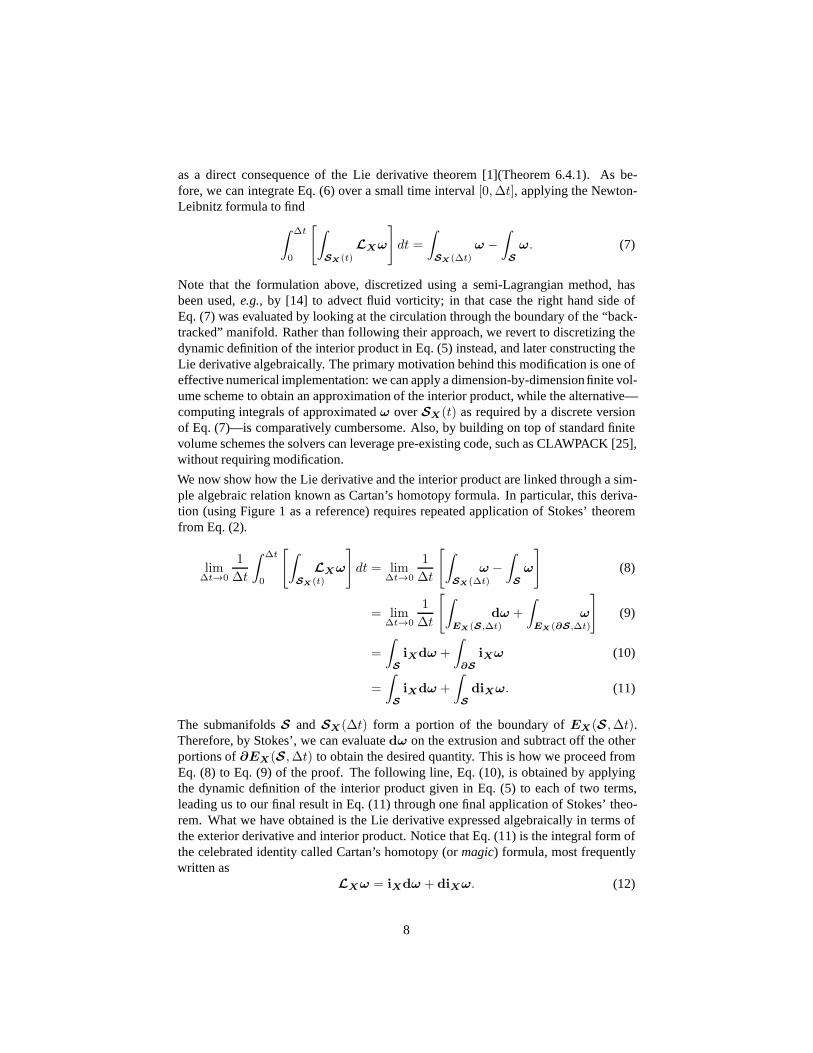
3.1 Towards a Dynamic Definition of Lie DerivativeInterior Product through Extrusion. As pointed out by [7], theextrusionof objectsunder the flow of a vector field can be used to give an intuitive dynamic definition ofthe interior product. IfM is ann-dimensional smooth manifold andX ∈ X(M) asmooth (tangent) vector field on the manifold, letS be ak-dimensional submanifoldonM with k < n. The flowϕ of the vector fieldX is simply a functionϕ : M ×R → M consistent with the one-parameter (time) group structure,that is, such thatϕ(ϕ(S, t), s) = ϕ(S, s + t) with ϕ(S, 0) = S for all s, t ∈ R. Now imaginethatS is carried by this flow ofX for a timet; we denote the resultant “flowed-out”submanifoldSX(t), which is equivalent to the image ofS under the mappingϕ, i.e.,SX(t) ≡ ϕ(S, t). The extrusionEX(S, t) is then the (k+1)-dimensional submanifoldformed by the advection ofS over the timet to its final positionSX(t): it is the“extruded” (or “swept out”) submanifold. This can be expressed formally as a union offlowed-out manifolds,

EX(S, t) =⋃

τ∈[0,t]

SX(τ)

6

where the orientation ofEX(S, t) is defined such that

∂EX = SX(t)− S −EX(∂S, t).

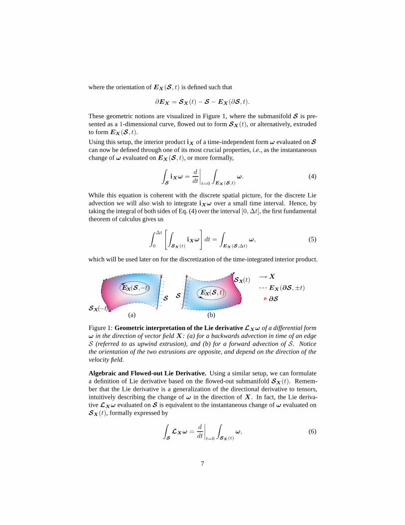
These geometric notions are visualized in Figure 1, where the submanifoldS is pre-sented as a1-dimensional curve, flowed out to formSX(t), or alternatively, extrudedto formEX(S, t).

Using this setup, the interior productiX of a time-independent formω evaluated onScan now be defined through one of its most crucial properties,i.e., as the instantaneouschange ofω evaluated onEX (S, t), or more formally,

∫

S

iXω =d

dt

∣

∣

∣

∣

t=0

∫

EX (S,t)

ω. (4)

While this equation is coherent with the discrete spatial picture, for the discrete Lieadvection we will also wish to integrateiXω over a small time interval. Hence, bytaking the integral of both sides of Eq. (4) over the interval[0,∆t], the first fundamentaltheorem of calculus gives us

∫ ∆t

0

[

∫

SX(t)

iXω

]

dt =

∫

EX(S,∆t)

ω, (5)

which will be used later on for the discretization of the time-integrated interior product.

X

EX(∂S ,±t)

∂S

SX(t)

EX(S, t)S

S

SX(−t)

EX(S,−t)

(a) (b)

Figure 1:Geometric interpretation of the Lie derivative LXω of a differential formω in the direction of vector fieldX: (a) for a backwards advection in time of an edgeS (referred to as upwind extrusion), and (b) for a forward advection of S. Noticethe orientation of the two extrusions are opposite, and depend on the direction of thevelocity field.

Algebraic and Flowed-out Lie Derivative. Using a similar setup, we can formulatea definition of Lie derivative based on the flowed-out submanifold SX(t). Remem-ber that the Lie derivative is a generalization of the directional derivative to tensors,intuitively describing the change ofω in the direction ofX. In fact, the Lie deriva-tive LXω evaluated onS is equivalent to the instantaneous change ofω evaluated onSX(t), formally expressed by

∫

S

LXω =d

dt

∣

∣

∣

∣

t=0

∫

SX(t)

ω, (6)

7

as a direct consequence of the Lie derivative theorem [1](Theorem 6.4.1). As be-fore, we can integrate Eq. (6) over a small time interval[0,∆t], applying the Newton-Leibnitz formula to find

∫ ∆t

0

[

∫

SX(t)

LXω

]

dt =

∫

SX(∆t)

ω −

∫

S

ω. (7)

Note that the formulation above, discretized using a semi-Lagrangian method, hasbeen used,e.g., by [14] to advect fluid vorticity; in that case the right handside ofEq. (7) was evaluated by looking at the circulation through the boundary of the “back-tracked” manifold. Rather than following their approach, we revert to discretizing thedynamic definition of the interior product in Eq. (5) instead, and later constructing theLie derivative algebraically. The primary motivation behind this modification is one ofeffective numerical implementation: we can apply a dimension-by-dimensionfinite vol-ume scheme to obtain an approximation of the interior product, while the alternative—computing integrals of approximatedω overSX(t) as required by a discrete versionof Eq. (7)—is comparatively cumbersome. Also, by building on top of standard finitevolume schemes the solvers can leverage pre-existing code,such as CLAWPACK [25],without requiring modification.

We now show how the Lie derivative and the interior product are linked through a sim-ple algebraic relation known as Cartan’s homotopy formula.In particular, this deriva-tion (using Figure 1 as a reference) requires repeated application of Stokes’ theoremfrom Eq. (2).

lim∆t→0

1

∆t

∫ ∆t

0

[

∫

SX(t)

LXω

]

dt = lim∆t→0

1

∆t

[

∫

SX(∆t)

ω −

∫

S

ω

]

(8)

= lim∆t→0

1

∆t

[

∫

EX(S,∆t)

dω +

∫

EX(∂S,∆t)

ω

]

(9)

=

∫

S

iXdω +

∫

∂S

iXω (10)

=

∫

S

iXdω +

∫

S

diXω. (11)

The submanifoldsS andSX(∆t) form a portion of the boundary ofEX(S,∆t).Therefore, by Stokes’, we can evaluatedω on the extrusion and subtract off the otherportions of∂EX(S,∆t) to obtain the desired quantity. This is how we proceed fromEq. (8) to Eq. (9) of the proof. The following line, Eq. (10), is obtained by applyingthe dynamic definition of the interior product given in Eq. (5) to each of two terms,leading us to our final result in Eq. (11) through one final application of Stokes’ theo-rem. What we have obtained is the Lie derivative expressed algebraically in terms ofthe exterior derivative and interior product. Notice that Eq. (11) is the integral form ofthe celebrated identity called Cartan’s homotopy (ormagic) formula, most frequentlywritten as

LXω = iXdω + diXω. (12)

8

By defining our discrete Lie derivative through this relation, we ensure the algebraicdefinition holds true in the discrete sense by construction.It also implies that the Liederivative can be directly defined through interior productand exterior derivative, with-out the need for its own discrete definition.

Upwinding the Extrusion We may rewrite the above notions using an “upwinded”extrusion (i.e., a cell extruded backwards in time) as well (see Fig. 1a). Forexample,Eq. (4) can be rewritten as

∫

S

iXω = −d

dt

∣

∣

∣

∣

t=0

∫

EX(S,−t)

ω. (13)

While this does not change the instantaneous value of the contraction, integratingEq. (13) over the time interval[0,∆t] now gives us

∫ ∆t

0

[

∫

SX(t)

iXω

]

dt = −

∫

EX (S,−∆t)

ω. (14)

Similar treatment for the remainder of the above can be done and Cartan’s formula canbe derived the same way, however by using these definitions inour following discretiza-tion we will obtain computations over upwinded regions equivalent to those computedby finite volume methods.

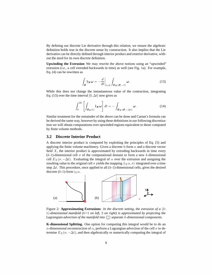
3.2 Discrete Interior ProductA discrete interior product is computed by exploiting the principles of Eq. (5) andapplying the finite volume machinery. Given a discretek-formα and a discrete vectorfield X , the interior product is approximated by extruding backwards in time every(k-1)-dimensional cellσ of the computational domain to form a newk-dimensionalcell EX(σ,−∆t). Evaluating the integral ofα over the extrusion and assigning theresulting value to the original cellσ yields the mapping〈iXα, σ〉 integrated over a timestep∆t. This procedure, once applied to all (k-1)-dimensional cells, gives the desireddiscrete (k-1)-form iXα.

(a) (b) z

xy

Figure 2: Approximating Extrusions : In the discrete setting, the extrusion of a(k-1)-dimensional manifold (k=1 on left, 2 on right) is approximated by projecting theLagrangian advection of the manifold into

(

nk

)

separatek-dimensional components.

K-dimensional Splitting. One option for computing this integral would be to do ann-dimensional reconstruction ofα, perform a Lagrangian advection of the cellσ to de-termineEX(σ,−∆t), and then algebraically or numerically computing the integral of

9

the reconstructedα over this extrusion. In fact, this is the idea behind the approach sug-gested in [21]. However, with the exception of whenk=n, such an approach does notallow us to directly leverage finite volume methods, as performing ann-dimensionalreconstruction of a form given only integrals overk-dimensional submanifolds wouldrequire a more general finite element framework. For simplicity and ease of imple-mentation we avoid this generalization and instead resort to projecting the extrusiononto the grid-alignedk-dimensional subspaces and then applying ak-dimensional fi-nite volume method to each of the

(

nk

)

projections. The integrals over the extrusionof σ from each dimension are then summed. Again, note that in the special case ofk = n no projection is required and we are left exactly with ann-dimensional finitevolume scheme. We have found that this splitting combined with a high-resolution fi-nite volume method, despite imposing at most first order accuracy, can still give highquality results with low numerical diffusion, while being able to leverage existing finitevolume solvers without modification. However, if truly higher order is required then afull-blown finite element method would most likely be required [21].

Finite Volume Evaluation. As hinted at in Section 2.3, we notice that the time integralof the flux of a density field being advected through a submanifoldσ is equivalent to theintegral of the density field over the backwards extrusion ofσ over the same amount oftime. In fact, some finite volume methods are derived using this interpretation, doing areconstruction of the density field, approximating the extrusion, and integrating the re-construction over this. However, many others are explainedby computing a numericalflux per face, and then multiplying by the time step∆t: this is still an approximation ofthe integral over the extrusion, taking the reconstructionto be a constant (the numericalflux divided byv) and the extrusion having lengthv∆t. Indeed the right hand side ofEq. (4) can be seen as analogous to the numerical flux, after which Eq. (5) becomesthe relationship between integrating the flux over time and the form over the extru-sion. Hence we may use any of the finite volume methods fork-dimensional densityadvection problems when computing the contraction of ak-form. The only differencehere is that rather than applying Stokes theorem and summingthe contributions back tothe originalk-cell (which will be done by the discrete exterior derivative in thediXω

term of the Lie derivative), the contraction simply stores the values on the (k-1)-cells,without the final sum.

3.3 Discrete Lie AdvectionWe now have all the ingredients to introduce a discrete Lie advection. Given ak-formα, we compute the (k+1)-form dα by applying the transpose of the incidence matrix∂k+1 toα as detailed in§2.2. We then compute thek-form iX(dα), and the (k-1)-formiXα. By applyingd to the latter form and summing the resultingk-form with the otherinterior product, we finally get an approximation of Cartan’s homotopy formula of theLie derivative. An explicit example of this will be given in the next section to betterillustrate the process and details.

4 Applications and ResultsWe now present a few direct applications of this discrete Lieadvection scheme. In ourtests we used upwinding one-dimensional WENO schemes for our contraction operator,

10

splitting even thek-dimensional problems into multiple one-dimensional ones. Wefound that when using high-resolution WENO schemes we couldobtain quality resultswith little numerical smearing despite this dimensional splitting.

A Note on Vector Fields. In this section we assume that vector fields are discretized bystoring their flux (i.e., contraction with the volume form) on all the(n−1)-dimensionalcells of anD regular grid, much like the Marker-And-Cell “staggered” grid setup [20].Evaluation of the vector fields at lower dimensional cells isdone through simple aver-aging of adjacent discrete fluxes. We pick this setup as it is one of the most commonly-used representations, but the vector fields can be given in arbitrary form with onlyminor implementation changes.

4.1 Volume Forms and0-FormsApplying our approach to volume forms (n-forms inn dimensions) we have

LXω = iXdω + diXω = diXω.

Note thatiXω is the numerical flux computed by the chosenn-dimensional finite vol-ume scheme whiled will then just assign the appropriate sign of this flux to eachcell’s update, and hence we trivially arrive at the chosen finite volume scheme with nomodification. Similarly, applying this approach to0-forms results in well-known finitedifference advection schemes of scalar fields. Indeed, we have in this case

LXω = iXdω + diXω = iXdω

as the contraction of a0-form vanishes. We are thus left withdω computing standardfinite differences of a node-based scalar field on edges, andiX then doing componen-twise upwind integration of reconstructions of these derivatives. Such techniques arecommon in scalar field advection, for example in the advection of level sets, and werefer the reader to [35, 36] and references therein for examples.

4.2 Advecting a1-Form in 2DThe novelty of this approach comes when applied tok-forms in n dimensions withn > k > 0. We first demonstrate the simplest such application of our method byadvecting a1-form by a static velocity field in 2D using the simple piecewise-constantupwinding finite volume advection. To illustrate the general approach we will explicitlywrite out the algorithm for this case. We will assume the velocity X is everywherepositive in bothx andy components to simplify the upwinding, andXx andXy will beused to represent the integrated flux through vertical and horizontal edges respectively.

Suppose we have a regular two-dimensional grid with square cells of sizeh2, and witheach horizontal edge oriented in the positivex direction and each vertical edge orientedin the positivey direction and numbered according to Fig 3. A discrete1-form ω isrepresented by its integral along each edge. Due to the Cartesian nature of the grid, thisimplies that thedx component of the form will be stored on horizontal edges and thedy component will be stored on vertical edges, and we representthese scalars asωx

i,j

andωyi,j for the integrals along the(i, j) horizontal and vertical edge respectively. The

11

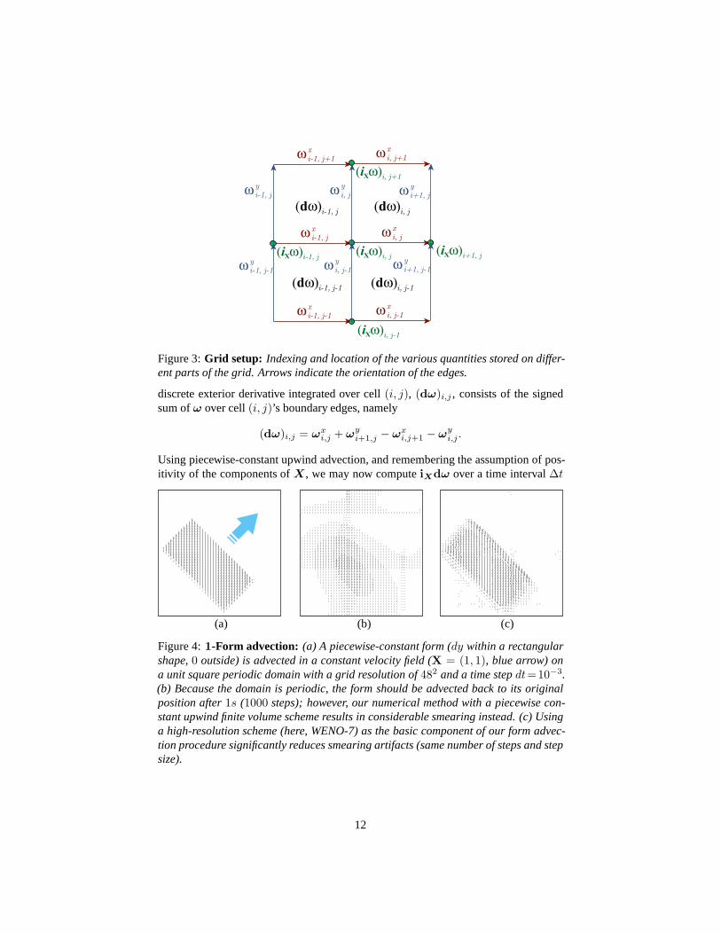
Figure 3:Grid setup: Indexing and location of the various quantities stored on differ-ent parts of the grid. Arrows indicate the orientation of theedges.

discrete exterior derivative integrated over cell(i, j), (dω)i,j , consists of the signedsum ofω over cell(i, j)’s boundary edges, namely

(dω)i,j = ωxi,j + ω

yi+1,j − ωx

i,j+1 − ωyi,j .

Using piecewise-constant upwind advection, and remembering the assumption of pos-itivity of the components ofX, we may now computeiXdω over a time interval∆t

(a) (b) (c)

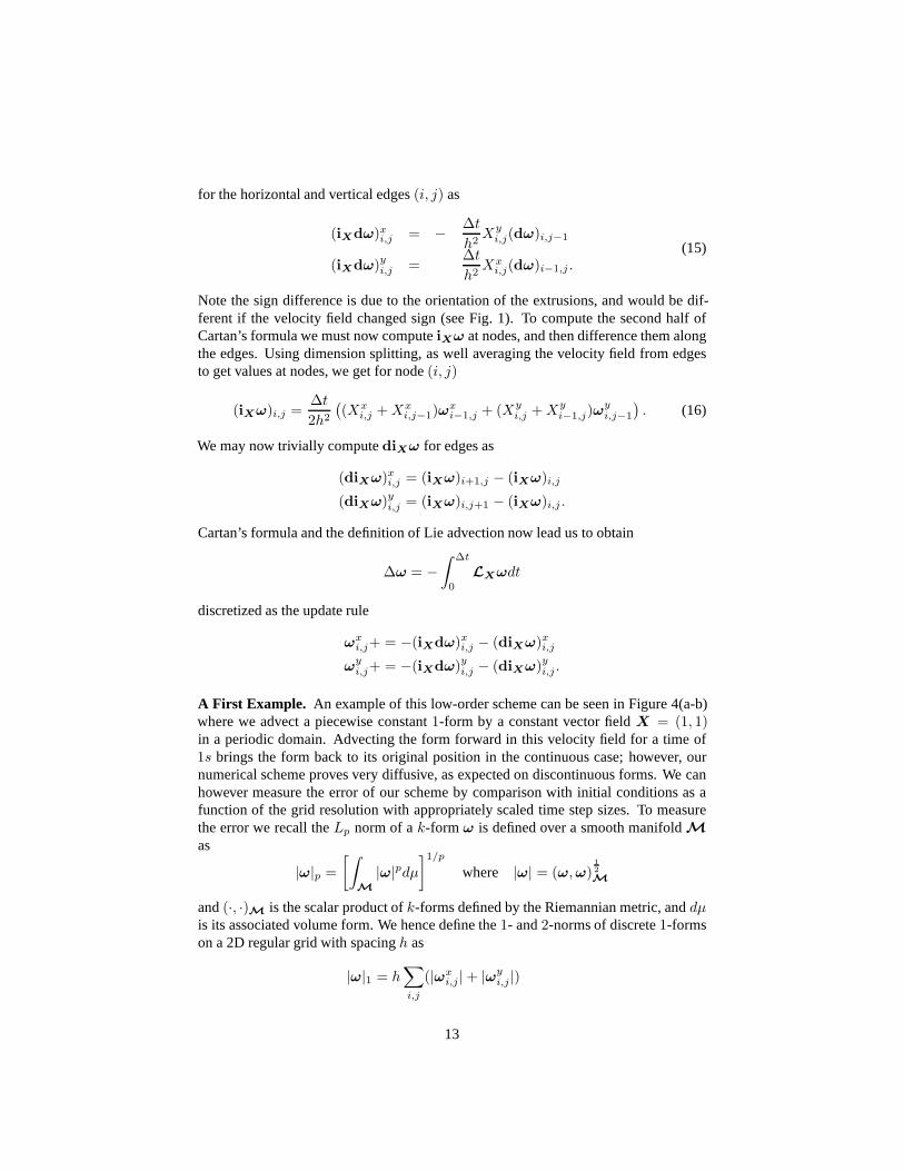
Figure 4:1-Form advection: (a) A piecewise-constant form (dy within a rectangularshape,0 outside) is advected in a constant velocity field (X = (1, 1), blue arrow) ona unit square periodic domain with a grid resolution of482 and a time stepdt=10−3.(b) Because the domain is periodic, the form should be advected back to its originalposition after1s (1000 steps); however, our numerical method with a piecewise con-stant upwind finite volume scheme results in considerable smearing instead. (c) Usinga high-resolution scheme (here, WENO-7) as the basic component of our form advec-tion procedure significantly reduces smearing artifacts (same number of steps and stepsize).

12

for the horizontal and vertical edges(i, j) as

(iXdω)xi,j = −∆t

h2Xy

i,j(dω)i,j−1

(iXdω)yi,j =∆t

h2Xx

i,j(dω)i−1,j .(15)

Note the sign difference is due to the orientation of the extrusions, and would be dif-ferent if the velocity field changed sign (see Fig. 1). To compute the second half ofCartan’s formula we must now computeiXω at nodes, and then difference them alongthe edges. Using dimension splitting, as well averaging thevelocity field from edgesto get values at nodes, we get for node(i, j)

(iXω)i,j =∆t

2h2

(

(Xxi,j +Xx

i,j−1)ωxi−1,j + (Xy

i,j +Xyi−1,j)ω

yi,j−1

)

. (16)

We may now trivially computediXω for edges as

(diXω)xi,j = (iXω)i+1,j − (iXω)i,j

(diXω)yi,j = (iXω)i,j+1 − (iXω)i,j .

Cartan’s formula and the definition of Lie advection now leadus to obtain

∆ω = −

∫ ∆t

0

LXωdt

discretized as the update rule

ωxi,j+ = −(iXdω)xi,j − (diXω)xi,j

ωyi,j+ = −(iXdω)yi,j − (diXω)yi,j .

A First Example. An example of this low-order scheme can be seen in Figure 4(a-b)where we advect a piecewise constant1-form by a constant vector fieldX = (1, 1)in a periodic domain. Advecting the form forward in this velocity field for a time of1s brings the form back to its original position in the continuous case; however, ournumerical scheme proves very diffusive, as expected on discontinuous forms. We canhowever measure the error of our scheme by comparison with initial conditions as afunction of the grid resolution with appropriately scaled time step sizes. To measurethe error we recall theLp norm of ak-form ω is defined over a smooth manifoldMas

|ω|p =

[∫

M

|ω|pdµ

]1/p

where |ω| = (ω,ω)1

2

M

and(·, ·)M is the scalar product ofk-forms defined by the Riemannian metric, anddµis its associated volume form. We hence define the1- and2-norms of discrete1-formson a 2D regular grid with spacingh as

|ω|1 = h∑

i,j

(|ωxi,j |+ |ωy

i,j |)

13

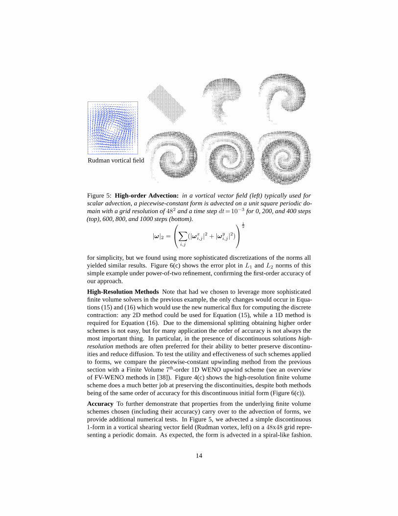
Rudman vortical field

Figure 5: High-order Advection: in a vortical vector field (left) typically used forscalar advection, a piecewise-constant form is advected ona unit square periodic do-main with a grid resolution of482 and a time stepdt=10−3 for 0, 200, and 400 steps(top), 600, 800, and 1000 steps (bottom).

|ω|2 =

∑

i,j

(|ωxi,j |

2 + |ωyi,j |

2)

1

2

for simplicity, but we found using more sophisticated discretizations of the norms allyielded similar results. Figure 6(c) shows the error plot inL1 andL2 norms of thissimple example under power-of-two refinement, confirming the first-order accuracy ofour approach.

High-Resolution Methods Note that had we chosen to leverage more sophisticatedfinite volume solvers in the previous example, the only changes would occur in Equa-tions (15) and (16) which would use the new numerical flux for computing the discretecontraction: any 2D method could be used for Equation (15), while a 1D method isrequired for Equation (16). Due to the dimensional splitting obtaining higher orderschemes is not easy, but for many application the order of accuracy is not always themost important thing. In particular, in the presence of discontinuous solutionshigh-resolutionmethods are often preferred for their ability to better preserve discontinu-ities and reduce diffusion. To test the utility and effectiveness of such schemes appliedto forms, we compare the piecewise-constant upwinding method from the previoussection with a Finite Volume7th-order 1D WENO upwind scheme (see an overviewof FV-WENO methods in [38]). Figure 4(c) shows the high-resolution finite volumescheme does a much better job at preserving the discontinuities, despite both methodsbeing of the same order of accuracy for this discontinuous initial form (Figure 6(c)).

Accuracy To further demonstrate that properties from the underlyingfinite volumeschemes chosen (including their accuracy) carry over to theadvection of forms, weprovide additional numerical tests. In Figure 5, we advected a simple discontinuous1-form in a vortical shearing vector field (Rudman vortex, left) on a48x48 grid repre-senting a periodic domain. As expected, the form is advectedin a spiral-like fashion.

14

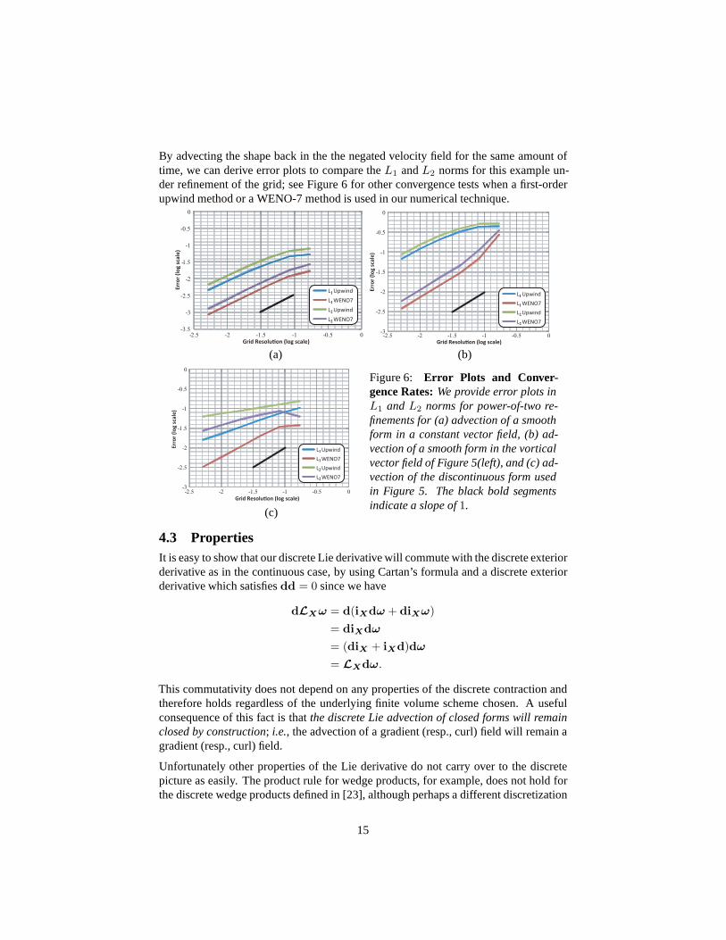
By advecting the shape back in the the negated velocity field for the same amount oftime, we can derive error plots to compare theL1 andL2 norms for this example un-der refinement of the grid; see Figure 6 for other convergencetests when a first-orderupwind method or a WENO-7 method is used in our numerical technique.

(a) (b)

(c)

Figure 6: Error Plots and Conver-gence Rates:We provide error plots inL1 andL2 norms for power-of-two re-finements for (a) advection of a smoothform in a constant vector field, (b) ad-vection of a smooth form in the vorticalvector field of Figure 5(left), and (c) ad-vection of the discontinuous form usedin Figure 5. The black bold segmentsindicate a slope of1.

4.3 PropertiesIt is easy to show that our discrete Lie derivative will commute with the discrete exteriorderivative as in the continuous case, by using Cartan’s formula and a discrete exteriorderivative which satisfiesdd = 0 since we have

dLXω = d(iXdω + diXω)

= diXdω

= (diX + iXd)dω

= LXdω.

This commutativity does not depend on any properties of the discrete contraction andtherefore holds regardless of the underlying finite volume scheme chosen. A usefulconsequence of this fact is thatthe discrete Lie advection of closed forms will remainclosed by construction; i.e., the advection of a gradient (resp., curl) field will remain agradient (resp., curl) field.

Unfortunately other properties of the Lie derivative do notcarry over to the discretepicture as easily. The product rule for wedge products, for example, does not hold forthe discrete wedge products defined in [23], although perhaps a different discretization

15

of the wedge product may prove otherwise. However, the nonlinearity of the discretecontraction operator along with the upwinding potentiallypicking different directionson simplices and their subsimplices makes designing a discrete analog satisfying thiscontinuous property challenging.

5 ConclusionsIn this paper we have introduced an extension of classical finite volume techniquesfor hyperbolic conservation laws to handle arbitrary discrete forms. A class of first-order finite-volume-based discretizations of both contraction and Lie derivative of ar-bitrary forms was presented, extending Discrete Exterior Calculus to include approx-imations to these operators. Low numerical diffusion is attainable through the use ofhigh-resolution finite volume methods. The advection of forms and vector fields areapplicable in a multitude of problems, including conservative interface advection andconservative vorticity evolution.Although finite volume methods can offer high resolution at arelatively low compu-tational cost, numerical diffusion is still present and canaccumulate over time. Inaddition, the numerical scheme we presented is not variational in nature,i.e., it is not(a priori) derived from a variational principle. These limitations are good motivationsfor future work.In the future, we also expect that extensions can be made to make truly high-orderand high-resolution discretizations of the contraction and Lie derivative throughn-dimensional reconstructions ofk-forms and extrusions: this would lead to a morestraightforward extension to simplicial meshes, as our current dimension splitting ap-proach does not obviously generalize to this framework despite recent progress in thisdirection [44, 27].

AcknowledgementsThis research was partially supported by NSF grants CCF-0811313& 0811373, CMMI-0757106 & 0757123, and DMS-0453145, and by the Center for theMathematics of Information at Caltech.

References[1] R. Abraham, J.E. Marsden, and T. Ratiu.Manifolds, Tensor Analysis, and Appli-

cations. Applied Mathematical Sciences Vol. 75, Springer, 1988.[2] D.N. Arnold, P.B. Bochev, R.B. Lehoucq, R.A. Nicolaides, and M. Shashkov, edi-

tors.Compatible Spatial Discretizations, volume 142 ofI.M.A. Volumes. Springer,2006.

[3] Douglas N. Arnold, Richard S. Falk, and Ragnar Winther. Finite element exteriorcalculus, homological techniques, and applications.Acta Numerica, 15:1–155,2006.

[4] Douglas N. Arnold, Richard S. Falk, and Ragnar Winther. Finite element exteriorcalculus: from Hodge theory to numerical stability. To appear inBull. Amer. Math.Soc., 74 pages, 2010.

[5] Pavel B. Bochev and James M. Hyman. Principles of MimeticDiscretizations ofDifferential Operators.I.M.A. Volumes, 142:89–119, 2006.

[6] Alain Bossavit. Computational Electromagnetism. Academic Press, Boston,1998.

16

[7] Alain Bossavit. Extrusion, Contraction : their Discretization via Whitney Forms.COMPEL: The International Journal for Computation and Mathematics in Elec-trical and Electronic Engineering, 22(3):470–480, 2003.

[8] William L. Burke. Applied Differential Geometry. Cambridge University Press,1985.

[9] Sean Carroll. Spacetime and Geometry: An Introduction to General Relativity.Pearson Education, 2003.

[10] Elie Cartan. Les Systemes Differentiels Exterieurs et leurs ApplicationsGeometriques. Hermann, Paris, 1945.

[11] Mathieu Desbrun, Eva Kanso, and Yiying Tong. Discrete Differential Forms forComputational Sciences. In Eitan Grinspun, Peter Schroder, and Mathieu Des-brun, editors,Discrete Differential Geometry, Course Notes. ACM SIGGRAPH,2006.

[12] T.F. Dupont and Y. Liu. Back-and-Forth Error Compensation and CorrectionMethods for Removing Errors Induced by Uneven Gradients of the Level SetFunction.Journal of Computational Physics, 190(1):311–324, 2003.

[13] V. Dyadechko and M. Shashkov. Moment-of-Fluid Interface Reconstruction.LANL Technical Report LA-UR-05-7571, 2006.

[14] Sharif Elcott, Yiying Tong, Eva Kanso, Peter Schroder, and Mathieu Desbrun.Stable, circulation-preserving, simplicial fluids.ACM Trans. Graph., 26(1):4,2007.

[15] Bjorn Engquist and Stanley Osher. One-Sided Difference Schemes and TransonicFlow. PNAS, 77(6):3071–3074, 1980.

[16] Harley Flanders.Differential Forms and Applications to Physical Sciences. DoverPublications, 1990.

[17] Theodore Frankel.The Geometry of Physics. Second Edition. Cambridge Univer-sity Press, United Kingdom, 2004.

[18] X. Gu and S.-T. Yau. Global Conformal Surface Parameterization. InSymposiumGeometry Processing, pages 127–137, 2003.

[19] Ernst Hairer, Christian Lubich, and Gerhard Wanner.Geometric Numerical Inte-gration: Structure-Preserving Algorithms for ODEs. Springer, 2002.

[20] F. H. Harlow and J. E. Welch. Numerical Calculation of Time-dependent ViscousIncompressible Flow of Fluid with Free Surfaces.Phys. Fluids, 8:2182–2189,1965.

[21] H. Heumann and R. Hiptmair. Extrusion contraction upwind schemes forconvection-diffusion problems. Technical Report SAM 2008-30, ETH Zurich,October 2008.

[22] D. J. Hill and D. I. Pullin. Hybrid Tuned Center-Difference-WENO Method forLarge Eddy Simulations in the Presence of Strong Shocks.J. Comput. Phys.,194(2):435–450, 2004.

[23] Anil N. Hirani. Discrete Exterior Calculus. PhD thesis, Caltech, May 2003.[24] Armin Iske and Martin Kaser. Conservative Semi-Lagrangian Advection on

Adaptive Unstructured Meshes.Numerical Methods for Partial Differential Equa-tions, 20(3):388–411, 2004.

[25] Randall J. Leveque. CLAWPACK, at http://www.clawpack.org. 1994-2009.[26] R.J. LeVeque.Finite Volume Methods for Hyperbolic Problems. Cambridge

Texts in Applied Mathematics. Cambridge University Press,2002.

17

[27] D. Levy, S. Nayak, C.W. Shu, and Y.T. Zhang. Central WENOSchemes forHamilton-Jacobi Equations on Triangular Meshes.J. Sci. Comput., 27:532–552,2005.

[28] X.D. Liu, S. Osher, and T. Chan. Weighted Essentially Non-oscillatory Schemes.J. Sci. Comput., 126:202–212, 1996.

[29] David Lovelock and Hanno Rund.Tensors, Differential Forms, and VariationalPrinciples. Dover Publications, 1993.

[30] Jerrold E. Marsden and Matthew West. Discrete Mechanics and Variational Inte-grators.Acta Numerica, 2001.

[31] Shigeyuki Morita.Geometry of Differential Forms. Translations of MathematicalMonographs, Vol. 201. Am. Math. Soc., 2001.

[32] James R. Munkres.Elements of Algebraic Topology. Addison-Wesley, MenloPark, CA, 1984.

[33] J.C. Nedelec. Mixed Finite Elements in 3D in H(div) and H(curl). SpringerLectures Notes in Mathematics, 1192, 1986.

[34] R. A. Nicolaides and X. Wu. Covolume Solutions of Three Dimensional Div-CurlEquations.SIAM J. Numer. Anal., 34:2195, 1997.

[35] Stanley Osher and Ronald Fedkiw.Level Set Methods and Dynamic ImplicitSurfaces, volume 153 ofApplied Mathematical Sciences. Springer-Verlag, NewYork, 2003.

[36] J. A. Sethian.Level Set Methods and Fast Marching Methods, volume 3 ofMono-graphs on Appl. Comput. Math.Cambridge University Press, Cambridge, 2ndedition, 1999.

[37] J. Shi, C. Hu, and C.W. Shu. A technique for treating negative weights in WENOschemes.J. Comput. Phys., 175:108–127, 2002.

[38] C.-W. Shu.Essentially non-oscillatory and weighted essentially non-oscillatoryschemes for hyperbolic conservation laws, volume 1697 ofLecture Notes in Math-ematics, pages 325–432. Springer, 1998.

[39] C.W. Shu and S. Osher. Efficient Implementation of Essentially non-OscillatoryShock Capturing Schemes.J. Sci. Comput., 77:439–471, 1988.

[40] Ari Stern, Yiying Tong, Mathieu Desbrun, and Jerrold E.Marsden. Variationalintegrators for maxwell’s equations with sources. InProgress in ElectromagneticsResearch Symposium, volume 4, pages 711–715, June 2008.

[41] V. A. Titarev and E. F. Toro. Finite-volume WENO schemesfor three-dimensional conservation laws.J. Comput. Phys., 201(1):238–260, 2004.

[42] Y. Tong, P. Alliez, D. Cohen-Steiner, and M. Desbrun. Designing Quadrangula-tions with Discrete Harmonic Forms. InProc. Symp. Geometry Processing, pages201–210, 2006.

[43] H. Whitney.Geometric Integration Theory. Princeton Press, Princeton, 1957.[44] Y.T. Zhang and C.W. Shu. High-Order WENO Schemes for Hamilton-Jacobi

Equations on Triangular Meshes.J. Sci. Comput., 24:1005–1030, 2003.

18