Discrete Event System Modeling and Simulationdelta.cs.cinvestav.mx/~lixo/Petrinets/notas.pdfThis is...

This is page i

Printer: Opaq

Discrete Event System Modeling and

Simulation

Xiaoou Li

Seccion de Computacion

Departamento de Ingenieria Electrica

Av.IPN 2508, A.P.14-740, Mexico D.F., 07360,

Mexico

email: [email protected]

Mayo 8, 2000

This is page 1

Printer: Opaq

1

Modeling Concepts and

Methodology–Petri Net Approach

1. Petri net basics (6hrs)

(a) History

(b) Petri net notation and definitions

(c) Petri net marking and state space

(d) Petri net dynamics

(e) Petri net language

(f) Examples, exercises

2. Analysis of Petri nets (4hrs)

(a) Problem classification (properties) (2hrs)

(b) The coverability tree (2hrs)

(c) Incidence matrix and state equation (1hrs)

(d) Simple reduction rules for analysis (1hrs)

3. Abbreviations, extensions and particular structures (6hrs)

(a) Classification

(b) Modeling by autonomous PNs

(c) Modeling by non-autonomous PNs

2 1. Modeling Concepts and Methodology–Petri Net Approach

4. Colored petri net and its applications (4hrs)

5. Fuzzy Petri net and its applications (2hrs)

6. Generalized stochastic Petri net and its applications (2hrs)

7. Hybrid Petri net and its applications (2hrs)

1.1 Petri Net Basics

1.1.1 History

Origin: Carl Adam Petri’s Dissertation ”Kommunikation mit Automaten.” the fac-

ulty of Mathematics and Physics at the Technical University of Darmstadt, West

Germany, 1962. Also English translation, ”Communication with Automata.” New

York: Griffiss Air Force Base. Tech. Rep. RADCTR-65-377, vol.1, Suppl. 1, 1966

1. 1962, Petri’s doctoral thesis, west Germany

2. –1970, early developments and applications of Petri nets are found in

(a) reports associated with the project ”Information System Theory Project

of Applied Data Research” (in USA)

(b) record of the 1970 Project MAC Conference on Concurrent Systems and

Parallel Computation

3. 1970–1975, the Computation structure Group at MIT was the most active.

In July, 1975, a conference on Petri Nets and Related Methods at MIT. (no

proceedings)

4. 1981, James L. Peterson, Petri net theory and the modeling of systems, Engle-

wood Cliffs, NJ: Prentice-Hall, Inc.

1. Modeling Concepts and Methodology–Petri Net Approach 3

5. 1985, W. Reisig, Petri nets, EATCS Monographs on Theoretical Computer

Science, Vol.4, NewYork: Springer Verlag

6. 1985–another series of international workshops, placed emphasis on timed

and stochastic nets and their applications to performance evaluation. (every

two years)

7. 1980–1989, European Workshops on Applications and Theory of Petri Nets

had been held every year at different location in Europe. Selected papers have

been published by Springer-Verlag as Advances in Petri Nets.

8. 1989–Petri Net Newsletter lists short abstracts of recent publications

1.1.2 Where can a Petri net apply to?

They can be applied informally to any area or system that can be described graphi-

cally like flow charts and that needs some means of representing parallel or concur-

rent activities.

Artificial Systems (or DEDS): manufacturing systems, software systems, traffic

systems, information systems, etc.

• Can not be described by traditional difference equation

• Characterized by states and events

• Can be modeled using models which are specially used in DEDS such as au-tomata, Petri nets, finite-state machines

• can be studied under those models mentioned above or using simulation method.

Two successful application areas : performance evaluation and communication

protocols.

Promising areas:


• modeling and analysis of distributed-software systems

• distributed-database systems

• concurrent and parallel programs

• flexible manufacturing/industrial control systems

• discrete-event systems

• multiprocessor memory systems

• data-flow computing systems

• fault-tolerant systems

• programmable logic and VLSI arrays

• asynchronous circuits and structures

• compiler and operating systems

• office-information systems

Other interesting applications: local-area networks, legal systems, human factors,

neural networks, digital filters, and decision models.

Comments on applications: Modeling, Seeking properties, Logic controller, Per-

formance evaluation

1.1.3 Petri net notation and definitions

Definition 1 (Petri net graph) A Petri net graph (or Petri net structure) is a

weighted bipartite graph


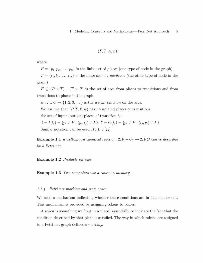
(P, T, A, w)

where

P = {p1, p2, . . . , pn} is the finite set of places (one type of node in the graph)T = {t1, t2, . . . , tm} is the finite set of transitions (the other type of node in the

graph)

F ⊆ (P × T ) ∪ (T × P ) is the set of arcs from places to transitions and from

transitions to places in the graph.

w : I ∪ O → {1, 2, 3, . . . } is the weight function on the arcs.We assume that (P, T, F, w) has no isolated places or transitions.

the set of input (output) places of transition tj:

·t = I(tj) = {pi ∈ P : (pi, tj) ∈ F}, t· = O(tj) = {pi ∈ P : (tj , pi) ∈ F}Similar notation can be used I(pi), O(pi).

Example 1.1 a well-known chemical reaction: 2H2+O2 → 2H2O can be described

by a Petri net.

Example 1.2 Products on sale

Example 1.3 Two computers use a common memory

1.1.4 Petri net marking and state space

We need a mechanism indicating whether these conditions are in fact met or not.

This mechanism is provided by assigning tokens to places.

A token is something we ”put in a place” essentially to indicate the fact that the

condition described by that place is satisfied. The way in which tokens are assigned

to a Petri net graph defines a marking.


¹¸º·

¹¸º· ¹¸

º·z:

-H2

O2

H2Ot22

(a)

¹¸º·

¹¸º· ¹¸

º·z:

-H2

O2

H2Ot22

(b)

t

t

t t

t

t t

FIGURE 1.1. First example: a chemical reaction

Formally, a marking x of a Petri net graph (P, T, F, w) is a function x : P → N =

{0, 1, 2, . . . }. Thus marking defines row vector x =[x(p1), x(p2), . . . , x(pn)], where nis the number of places in the Petri net. The ith entry of this vector indicates the

number of tokens in place pi, x(pi) ∈ N.

Definition 2 (Marked Petri net) A marked Petri net is a five-tuple (P, T, F, w, x)

where (P, T, F,w) is a Petri net graph and x is a marking of the set of places P ;

x =[x(p1), x(p2), . . . , x(pn)] ∈ Nn is the row vector associated with x.

For simplicity, we shall henceforth refer to a marked Petri net as just a Petri net.

The state of a Petri net is defined to be its marking row vector x =[x(p1), x(p2), . . . , x(pn)].

The state spaceX of a Petri net with n places is defined by all n−dimensional vectorswhose entries are non-negative integers, that is X ∈ Nn.

Definition 3 (enabled transition) A transition tj ∈ T in a Petri net is said to beenabled if

x(pi) ≥ w(pi, tj) for all pi ∈ I(tj)


µ´¶³µ´¶³ ?

?R

rr rr r rProducts

to be sold

Arrivalof a buyer

waiting

buyers

Sale

µ´¶³µ´¶³ ?

?R

rr rr r rProducts

to be sold

Incoming

of a buyer

waiting

buyers

Sale

µ´¶³r?

6

AllowedIncomings

(a) (b)

FIGURE 1.2. Second example: products on sale

In words, transition tj in the Petri net is enabled when the number of tokens in pi

is at least as large as the weight of the arc connecting pi to tj , for all places pi that

are input to transition tj .

Since places are associated with conditions regarding the occurrence of a transi-

tion, then a transition is enabled when all the conditions required for its occurrence

are satisfied; tokens are the mechanism used to determine satisfaction of conditions.

1.1.5 Petri Net Dynamics (Execution rules)

The state transition mechanism is provided by moving tokens through the net and

hence changing the state of the Petri net. When a transition is enabled, we say that

it can fire. The state transition function of a Petri net is defined through the change

in the state of the Petri net due to the firing of an enabled transition.

Definition 4 (Petri net dynamic) The state transition function, f : Nn× → Nn,

of Petri net (P, T, F, w, x) is defined for transition tj ∈ T if and only if

x(pi) ≥ w(pi, tj) for all pi ∈ I(tj)


If f(x, tj) is defined, then we set

x0(pi) = x(pi)− w(pi, tj) + w(tj, pi), i = 1, . . . , n (1.1)

Remark 1.1 The number of tokens need not be conserved upon the firing of a tran-

sition in a Petri net. Since it is entirely possible thatXpi∈P

w(tj , pi) >Xpi∈P

w(pi, tj) orXpi∈P

w(tj, pi) <Xpi∈P

w(pi, tj)

In general, it is entirely possible that after several transition firings, the resulting

state is x =[0, 0, . . . , 0], or that the number of tokens in one or more places grows

arbitrarily large after an arbitrarily large number of transition firings.

Example 1.4 (Firing of transitions)

Definition 5 (reachable states) The set of reachable states of Petri net (P, T, F, w, x)

is

R[(P, T, F, w, x)] := {y ∈ Nn : ∃s ∈ T ∗(f(m, s) = y)}.

(example fig4 4)

State Equations –a convenient algebraic tool

Let us define the firing vector u , an m−dimensional row vector of the form

u = [0, . . . 0, 1, 0, . . . , 0]

where the only 1 appears in the jth position, j ∈ {1, . . . ,m}, to indicate that factthat the jth transition is currently firing.

The incidence matrix of a Petri net, A, an m × n matrix whose (j, i) entry is ofthe form

aji = w(tj, pi)− w(pi, tj).


Using the incidence matrix A , we can now write a vector state equation

x0= x+ u ·A (1.2)

which describes that state transition process as a result of an ”input” u , that

is, a particular transition firing. The ith equation in 1.2 is precisely equation 1.1.

Therefore, f(x, tj) = x+ u ·A, where f(x, tj) is the transition function.The state equation provides a convenient algebraic tool and an alternative to

purely graphical means for describing the process of firing transitions and changing

the state of a Petri net.

Example 1.5 (State equation) consider the Petri net of figure1.5(a), with the initial

state x0 = [2, 0, 0, 1]. We can first write down the incidence matrix by inspection of

the Petri net graph, which in this case is

A =

−1 1 1 0

0 0 −1 1

−1 0 −1 −1

.The (1,2) entry, for example is given by w(t1, p2)−w(p2, t1) = 1−0. Using equation1.2, the state equation when transition t1 fires at state x0 is

x1 = [ 2 0 0 1 ] + [ 1 0 0 ]

−1 1 1 0

0 0 −1 1

−1 0 −1 −1

= [ 2 0 0 1 ] + [ −1 1 1 0 ] = [ 1 1 1 1 ]

which is precisely what we obtained in example (??). Similarly, we can determine x2

as a result of firing t2 next, as in fig. 1.5(c):

x2 = [ 1 1 1 1 ] + [ 0 1 0 ]

−1 1 1 0

0 0 −1 1

−1 0 −1 −1

= [ 1 1 0 2 ]


1.1.6 Petri net Language

Definition 6 (Labeled Petri net) A labeled Petri net N is an eight-tuple

N = (P, T, F, w,E, `,x0,Xm)

where

(P, T, F,w) is a petri net graph

E is the event set for transition labeling

` : T → E is the transition labeling function

x0 ∈ Nn is the initial state of the net (i.e., the initial number of tokens in each

place)

Xm ⊆ Nn is the set of marked states of the net.

In Petri net graphs, the label of a transition is indicated next to the transition.

Definition 7 (Language generated and marked) The language generated by labeled

Petri net N = (P, T, F, w,E, `,x0,Xm) is

L(N) := {`(s) ∈ E∗ : s ∈ T ∗ and f(x0, s) is defined}.

The language marked by N is

Lm(N) := {`(s) ∈ L(N) : s ∈ T ∗ and f(x0, s) ∈ Xm}.

(This definition uses the extended form of the transition labeling function ` : T ∗ →E∗; this extension is done in the usual manner.)

These definitions are completely consistent with the corresponding definitions for

automata. The language L(N) represents all strings of transition labels that areobtained by all possible (finite) sequences of transition firings in N , starting in the

initial state x0 of N ; The marked language Lm(N) is the subset of these strings thatleave the Petri net in a state that is a member of the set of marked states given in

th definition of N .


The class of languages that can be represented by labeled Petri nets is

PNL := {K ⊆ E∗ : ∃N = (P, T, F,w,E, `,x0,Xm)[Lm(N) = K]}.

This is a general definition and the properties of PNL depend heavily on the specificassumptions that are made about ` (e.g., injective or not) and Xm (e.g., finite or

infinite).

1.1.7 Modeling with Petri net (examples)

Events and Conditions

The simple Petri net view of a system concentrates on two primitive concepts: events

and conditions.

System Petri net

Conditions Places

Events Transitions

Preconditions of an event Inputs of the corresponding transition

Postconditions of an event Outputs of the corresponding transition

Example 1.6 (a simple machine shop modeling problem) The machine shop

waits until an order appears and then machines the ordered parts and sends it for

delivery.

The conditions for the system are:

1. (a) The machine shop is waiting

(b) An order has arrived and is waiting

(c) The machine shop is working on the order

(d) The order is complete

The events would be


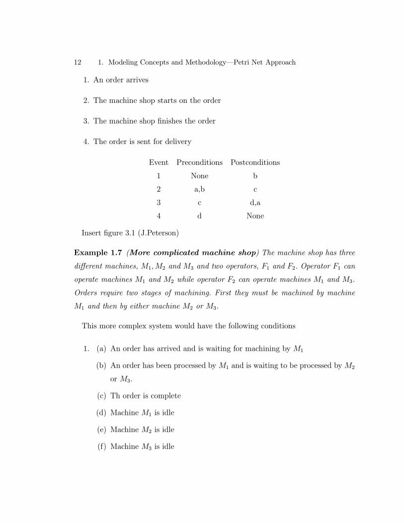
1. An order arrives

2. The machine shop starts on the order

3. The machine shop finishes the order

4. The order is sent for delivery

Event Preconditions Postconditions

1 None b

2 a,b c

3 c d,a

4 d None

Insert figure 3.1 (J.Peterson)

Example 1.7 (More complicated machine shop) The machine shop has three

different machines, M1,M2 and M3 and two operators, F1 and F2. Operator F1 can

operate machines M1 and M2 while operator F2 can operate machines M1 and M3.

Orders require two stages of machining. First they must be machined by machine

M1 and then by either machine M2 or M3.

This more complex system would have the following conditions

1. (a) An order has arrived and is waiting for machining by M1

(b) An order has been processed by M1 and is waiting to be processed by M2

or M3.

(c) Th order is complete

(d) Machine M1 is idle

(e) Machine M2 is idle

(f) Machine M3 is idle


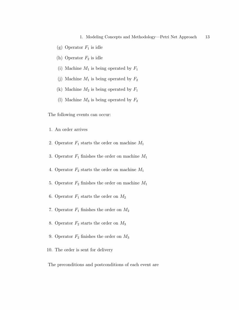
(g) Operator F1 is idle

(h) Operator F2 is idle

(i) Machine M1 is being operated by F1

(j) Machine M1 is being operated by F2

(k) Machine M2 is being operated by F1

(l) Machine M3 is being operated by F2

The following events can occur:

1. An order arrives

2. Operator F1 starts the order on machine M1

3. Operator F1 finishes the order on machine M1

4. Operator F2 starts the order on machine M1

5. Operator F2 finishes the order on machine M1

6. Operator F1 starts the order on M2

7. Operator F1 finishes the order on M2

8. Operator F2 starts the order on M3

9. Operator F2 finishes the order on M3

10. The order is sent for delivery

The preconditions and postconditions of each event are


Events Preconditions Postconditions

1 None a

2 a,g,d i

3 i g,d,b

4 a,h,d j

5 j b,h,d

6 b,g,e k

7 k c,g,e

8 b,f,h l

9 l c,f,h

10 c None

Insert figure 3.2 (J. Peterson)

In this section, several simple examples are given to introduce the reader to some

basic concepts of Petri nets that are useful in modeling.

Petri Net Model for Queueing Systems

Insert figure 4.5

a: customer arrival

s: service starts

c: service completes and customer departs

(a) Simple queueing system

(b) Petri net model of simple queueing system in initial state [0,1,0]

(c) Petri net model of simple queueing system with initial state [0,1,0] after firing

sequence {a,s,a,a,c,s,a}.

Finite-State Machines

Consider a vending machine which accepts either nickels or dimes and sells 15/c

or 20/c candy bars. For simplicity, suppose the vending machine can hold up to 20/c.


Then, the state diagram of the machine can be represented by a Petri net.

Note that each transition in this net has exactly one incoming arc and exactly

one outgoing arc. The subclass of Petri net with this property is known as state

machines. State machines allow the representation of decisions (or conflicts, choice),

but not the synchronization of parallel activities.

Example 1.8 (Dataflow Computation)

Insert figure 8 (murata)

Concurrency and Conflict

Petri net features:

Concurrency (or parallelism): In Petri net model, two events which are both en-

abled and do not interact may occur independently. There is no need to synchronize

events unless it is required by the underlying system which is being modeled. When

synchronization is needed, it is easy to model this also. Thus, Petri nets would seem

ideal for modeling systems of distributed control with multiple processes executing

concurrently in time.

Asynchronous: There is no inherent measure of time or the flow of time in a Petri

net. This reflects a philosophy of time which states that the only important property

of time, from a logical point of view, is in defining a partial ordering of the occurrence

of events. Events take variable amounts of time in real life, and this variability is

reflected in the Petri net model by not depending on a notion of time to control the

sequence of events. The Petri net structure itself contains all necessary information

to define the possible sequence of events. (example)

Nondeterminism: The order of occurrence of the events is one of possibly many

allowed by the basic structure.

Instaneous: taking zero time. and the occurrences of two events cannot happen

simutaneously.


1.2 Analysis of Petri Net

1.2.1 Problem classification (properties)

After modeling systems with Petri nets, an obvious question is ”What can we do

with the models?” A major strength of Petri nets is their support for analysis of

many properties and problems associated with concurrent systems.

Two types of properties can be studied with a Petri net model:

1. those which depend on the initial marking (refered as marking-dependent or

behavioral properties)

2. those which independ on the initial marking (structural properties)

The following are some of the key issues related to the logical behavior of Petri

nets. These issues relate primarily to desirable properties that often have their direct

analogs in CVDS. Many of these properties are motivated by the fact that Petri net

models are often used in resource sharing environments where we would like to

ensure efficient and fair usage of the resources.

Reachability

A markingMn is said to be reachable from a markingM0 if there exists a sequence

of firings that transforms M0 to Mn.

σ =M0 t1 M1 t2 M2 · · · tn Mn : a firing or occurrence sequence. or simply σ = t1

t2 · · · tn.M0[σ > Mn : Mn is reachable from M0 by σ.

R(N,M0) : the set of all possible markings reachable from M0 in a net (N,M0).

or simply R(M0).

L(N,M0) : the set of all possible firing sequences from M0 in a net (N,M0). or

simply L(M0).

Boundedness


In many instances, tokens represent customers in a resource sharing system. For

example, queue.......

Clearly, allowing queues to grow to infinity is undesirable, since it means that

customers wait forever to access a server. In classical system theory, a state variable

that is allowed to grow to infinity is generally an indicator of instability in the

system. Similarly here, unbounded growth in state components (markings) leads to

some form of instability.

Boundedness refers to the property of a place to maintain a number of token that

never exceeds a given positive in teger.

Definition 8 (boundedness, safe) A Petri net (N,M0) is said to be k-bounded or

simply bounded if the number of tokens in each place does not exceed a finite number

k for any marking reachable from M0, i.e., M(pi) ≤ k for every place p and everymarking M ∈ R(M0). A Petri net is said to be safe if it is 1-bounded.

Given a DEDS modeled as a Petri net, a boundednessproblem consists of checking

if the net is bounded and determining a bound. If boundedness is not satisfied, then

our task may be to alter the model so as to ensure boundedness. If the Petri net

is bounded, then it can be transformed into an equivalent finite-state automaton,

allowing the application of the analysis techniques for finite-state automata, if so

desired.

Liveness

The concept liveness is closely related to the complete absence of deadlocks in

operating systems.

Definition 9 (liveness) A Petri net (N,M0) is said to be live if, no matter what

marking has been reached from M0 , it is possible to ultimately fire any transition of

the net by progressing through some further firing sequence.

This means that a live Petri net guarantees deadlock-free operation, no matter


what firing sequence is chosen.

Liveness is an ideal property for many systems. However, it is impractical and too

costly to verify this strong property for some systems such as the operating system

of a large computer. Thus, we relax the liveness condition and define different levels

of liveness as follows.

A transition t in a Petri net (N,M0) is said to be :

0) dead (L0-live) if t can never be fired in any firing sequence in L(M0)

1) L1-live (potentially firable) if t can be fired at least once in some firing sequence

in L(M0)

2) L2-live if given any positive integer k, t can be fired at least k times in some

firing sequence in L(M0)

3) L3-live if t appears infinitely, often in some firing sequence in L(M0)

4) L4-live or live if t is L1-live for every marking M in R(M0)

It is easy to see the following implications: L4-liveness=⇒L3-liveness=⇒L2-liveness=⇒L1-liveness.

Insert figure 4.10

Reversibility and Home State

Definition 10 (reversibility) A Petri net (N,M0) is said to be reversible if, for each

marking M in R(M0), M0 is reachable from M .

Thus, in a reversible net one can always get back to the initial marking or state. In

many applications, it is not necessary to get back to the initial state as long as one

can get back to some (home) state. Therefore, we relax the reversibility condition

and define a home state.

A marking M´is said to be a home stateif, for each marking M in R(M0) , M0 is

reachable from M .

Note that boundedness, liveness, and reversibility are independent of each other.

For example


Insert fig. 17 (murata)

Coverability

Definition 11 (coverability) A marking M in a Petri net (N,M0) is said to be

coverable if there exists a marking M0in R(M0) such that M

0(p) ≥ M(p) for each

p in the net.

Coverability is closely related to L1-liveness (potential firability). Let M be the

minimum marking needed to enable a transition t . Then t is dead (not L1-live) if

and only if M is not coverable. That is, t is L1-live if and only if M is coverable.

Persistence

Definition 12 (persistent) A Petri net (N,M0) is said to be persistent if, for any

two enabled transitions, the firing of one transition will not disable the other.

A transition in a persistent net, once it is enabled, will stay enabled until it fires.

The notion of persisitence is useful in the context of parallel program schemata and

speed-independent asynchronous circuits.

Persistency is closely related to conflict-free nets, and a safe persistent net can be

transformed into a marked graph by duplicating some transitions and places. Note

that all marked graphs are persistent, but not all persistent nets are marked graphs.

For example, ....fig.17(c)

Synchronic Distance

It is a metric closely related to a degree of mutual dependence between two events

in a condition/event system.

Definition 13 (synchronic distance)The synchronic distance between two transi-

tions t1 and t2 in a Petri net (N,M0) is defined by

d12 = maxσ

¯−σ(t1)− −

σ(t2)¯


where σ is a firing sequence starting at any marking M in R(M0) and−σ(ti) is the

number of times that transition ti, i = 1, 2 fires in σ.

For example, in Fig. 17(d)d12 = 1, d34 = 1, d13 =∞.The synchronic distance represents a well-defined metric for condition/event nets

and marked graphs. However, there are some difficulties when it is applied to more

general class of Petri nets.

Fairness

Two transitions t1 and t2 are said to be in a bounded-fair (or B-fair) relation if

the maximum number of times that either one can fire while the other is not firing

is bounded. A Petri net (N,M0) is said to be a B-fair net if every pair of transitions

in the net are in a B-fair relation.

A firing sequence σ is said to be unconditionally (globally) fair if it is finite or every

transition in the net appears infinitely often in σ. A Petri net is said to be an un-

conditionally fair net if every firing sequence σ from M in R(M0) is unconditionally

fair.

Relationships: every B-fair net is an unconditionally-fair net and every bounded

unconditionally-fair net is a B-fair net. For example...

• fig. 17(h) is a B-fair net as well as an unconditionally-fair net.

• Fig. 17(d) is neither a B-fair net nor an unconditionally-fair net, since t3 andt4 will not appear in an infinite firing sequence σ = t2t1t2t1 · · ·

• The unbounded net (fig. 17(c)) is an unconditionally fair net but not a B-fairnet


Analysis Methods:

1. The reachability tree

involves essentially the enumeration of all reachable markings or their coverable

markings. It should be able to apply to all classes of nets, but is limited to ”small”

nets due to the complexity of the state-space explosion.

2. Incidence matrix and state equation

3. Simple reduction rules for analysis

These two techniques are powerful bu t in many cases they are applicable only to

special subclasses of Petri nets or special situations.

1.2.2 The coverability tree

Tree representation of the markings. Nodes represent markings generated from M0

(the root) and its successors, and each arc represents a transition firing, which

transforms one marking to another. examples: simple reachability tree, or infinite

reachability tree.

Insert Fig 4.11, fig4.12 (DES)

Notations:

1. Root node This is the first node of the tree, corresponding to the initial state

of the given Petri net. For example, fig4.12, [1,0,0,0]

2. Terminal node. This is any node from which no transition can fire. For example,

fig 4.12, [0,0,1,1]

3. Duplicate node. This is a node identical to a node already in the tree. For

example, Fig 4.11, [1,1,0]

4. Node dominance. Let M = [m(p1), . . . ,m(pn)] and M0= [m

0(p1), . . . ,m

0(pn)]

be two markings, i.e., nodes in the coverability tree. We will say that ”M

dominates M0,” denoted by M >d M

0, if the following two conditions hold:


(a) m(pi) ≥ m0(pi), for all i = 1, . . . , n

(b) m(pi) > m0(pi), for at least some i = 1, . . . , n for example, Fig. 4.12

5. The symbol ω. This may be thought of as ¨infinity¨in representing the mark-

ing of an unbounded place. We use ω when we identify a node dominance

relationship in the coverability tree. ω has the properties that for each integer

n, ω > n, ω ± n = ω and ω ≥ ω. As an example, in Fig. 4.12

Coverability Tree Construction Algorithm

Step 1: Initialize M =M0 (initial marking)

Step 2: For each new node, M , evaluate the transition function f(M, tj) for all

tj ∈ T :Step 2.1: If f(M, tj) is undefined for all tj ∈ T (i.e., no transition is enabled

at marking M), then M is a terminal node.

Step 2.2: If f(M, tj) is defined for some tj ∈ T, creat a new node M 0=

f(M, tj). Then:

Step 2.2.1: If m(pi) = ω for some pi , set m0(pi) = ω

Step 2.2.2: If there exists a node M00in the path from the root

node M0 (included) to M such that M0>d M

00, set m

0(pi) = ω for all pi such that

m0(pi) > m

00(pi)

Step 2.2.3: Otherwise, set m0(pi) = f(M, tj)

Step 3: If all new nodes are either terminal or duplicate nodes, stop.

The coverability tree for a Petri net (N,M0) is constructed by the following algo-

rithm

Step 1) Label the initial marking M0 as the root and tag it ”new”.

Step 2) While ”new” markings exist, do the following:

Step 2.1) Select a new marking M.

Step 2.2) If M is identical to a marking on the path from the root to M , then

tag M ”old” and go to another new marking.


Step 2.3) If no transitions are enabled at M , tag M ”dead-end”.

Step 2.4) While there exist enabled transitions at M , do the following for each

enabled transition t at M :

Step 2.4.1) Obtain the marking M0that results from firing t at M .

Step 2.4.2) On the path from the root to M if there exists a marking M´

such that M´(p) ≥ M´(p) for each place p and M0 6= M´, i.e., M´ is coverable, then

replace M0(p)by ω for each p such that M´(p) > M´(p).

Step 2.4.3) Introduce M0as a node, draw an arc with label t from M to

M 0, and tag M0”new”.

ω may be thought as ”infinity”.

Example

Insert Fig. 16, fig. 18 (murata)

For a bounded Petri net, the coverability tree is also called the reachability tree

since it contains all possible markings.

Application of the Coverability Tree

Some of the properties that can be studied by using the coverability tree T for a

Petri net (N,M0) are the folllowing:

Boundedness, safety, and blocking problems

1) A net (N,M0) is bounded and thus R(M0) is finite iff (if and only if) ω does

not appear in any node labels in T .

2) A net (N,M0) is safe iff 0´s and 1´s appear in node labels in T .

3) A transition is dead iff it does not appear as an arc label in T .

Coverability problems

4) If M is reachable from M0, then there exists a node labeled M0such that

M ≤M 0.

Conservation problems


Disadvantage (Limitation): an exhaustive method. Because of the information

lost by the use of the symbol ω (which may represent only even or odd numbers,

increasing or decreasing numbers, etc.), the reachability and liveness problems can-

not be solved by the coverability tree method alone. For example, Fig 19(a) and (b)

have the same coverability tree, Yet, Fig 19(a) is a live net, while fig 19(b) is not

live.

Insert fig. 19 (murata)

1.2.3 Incidence matrix and state equation

State equation can be used to address problems such as state reachability and con-

servation. It provides an algebraic alternative to the graphical methodology based

on the coverability tree, and it can be quite powerful in identifying structural prop-

erties that are mostly dependent on the topology of the Petri net graph captured in

the incidence matrix A.

Necessary Reachability Condition: Supposethat a destination markingMd is reach-

able from M0 through a firing sequence {u1, u2, . . . , ud}. Writing the state equationfor i = 1, 2, . . . , d and summing them, we obtain

Md =M0 +AT

dXk=1

uk (1.3)

which can be written as

Ax = ∆M (1.4)

where ∆M = Md − M0 and x =dPk=1

uk. Here x is an n × 1 column vector ofnonnegative integers and is called the firing count vector. The ith entry of x denotes

the number of times that transition i must fire to transform M0 to Md. It is well

known that a set of linear algebraic equations has a solution x iff ∆M is orthogonal

to every solution y of its homogeneous system,

Ay = 0 (1.5)


Let r be the rank of A, and partition A in the following form:

A =

m− r r

←→ ←→ A11 A12

A21 A22

l rl n− r

(1.6)

where A12 is a nonsingular square matrix of order r. A set of (m − r) linearlyindependent solution y for (1.5) can be given as tha (m − r) rows of the following(m− r)×m matrix Bf :

Bf = [Iµ : −AT11(AT12)−1] (1.7)

where Iµ is the identity matrix of order µ = m − r. Note that ABTf = 0. That is,the vector space spanned by the row vectors of Bf . Now, the condition that ∆M is

orthogonal to every solution for Ay = 0 is equivalent to the following condition:

Bf∆M = 0 (1.8)

Thus, if Md is reachable from M0, then the firing counter vector x must exist and

(1.8) must hold. Therefore, we have the following necessary condition for reachability

in an unrestricted Petri net.

Theorem 1.1 If Md is reachable from M0 in a Petri net (N,M0), then Bf∆M = 0,

where ∆M =Md −M0 and Bf is given by 1.7.

Corollary 1.1 In a Petri net (N,M0), a marking Md is not reachable from M0( 6=Md) if their difference is a linear combination of the row vectors of Bf , that is

∆M = BTf z

where z is a nonzero µ× 1 column vector.


Example 1.9 For the Petri net shown in Fig 1.8, the state equation is illustrated

below, where the transition t3 fires to result in the marking M1 = (3 0 0 2)T from

M0 = (2 0 1 0)T :

3

0

0

2

=2

0

1

0

+−2 1 1

1 −1 0

1 0 −10 −2 2

0

0

1

.The Incidence matrix A is of rank 2 and can be partitioned in the form of (1.6),

where

A11 =

−2 1

1 −1

and A12 =

1 0

0 −2

.Thus, the matrix Bf can be found by (1.7):

Bf =

1 0 2 1/2

0 1 −1 −1/2

.It is easy to verify that Bf∆M = 0 holds for ∆M =M1 −M0 = (1 0 −1 2)T .

T-invariant and P-invariant

An integer solution x of the homogeneous equation (∆M = 0 in (1.4))

ATx = 0 (1.9)

is called a T-invariant, and an integer solution y of the transposed homogeneous

equation Ay = 0 is called a P-invariant.

Study structural properties with T-invariant and P-invariant:

Conservativeness: A Petri net N is said to be (patially) conservative if there exists

a positive integer y(p) for every (some ) place p such that the weighted sum of tokens,

MTy =MT0 y = a constant, for every M ∈ R(M0) and for any fixed initial marking

M0. It is easy to see that


Theorem 1.2 A Petri net N is (partially) conservative iff there exists an m-vector

of positive (nonnegative) integers such that Ay = 0, y 6= 0. (a positive P-invariant.)

Proof.

M =M0 + ATx, x = 0

Consider the inner product of M and y

MTy =MT0 y + x

TAy

MTy =MT0 y = a constant⇐⇒ Ay = 0, y 6= 0

Consistency: A Petri net N is said to be (patially) consistent if there exists a

marking M0 and a firing sequence σ from M0 back to M0 such that every (some)

transition occurs at least once in σ.

Theorem 1.3 A Petri net N is said to be (patially) consistent if there exists an

n-vector of positive (nonnegative) integers such that ATx = 0, x 6= 0. (a positive

T-invariant.)

Proof. Suppose a Petri net is consistent. Then from (1.3) there exists an x > 0

such that M0 = M0 + ATx or ATx = 0. Conversely, suppose x > 0 , ATx = 0.

Choose M0 and M large enough that M −M0 = ATx = 0, so that a firing sequence

σ, such that−σ = x, can be repeated.

Theorem 1.4 An m-vector y is an P-invariant iffMTy =MT0 y for any fixed initial

marking M0 and any M in R(M0).

Theorem 1.5 An n-vector x = 0 is a T-invariant iff there exists a marking M0

and a firing sequence σ from M0 back to M0 with its firing count vector−σ equal to

x.


The set of places (transitions) corresponding to nonzero entries in an P-invariant

y ≥ 0 (T-invariant x ≥ 0) is called the support of an invariant and is denoted bykyk (kxk). A support is said to be minimal if no proper nonempty subset of the

support is also a support. An invarient (vector) y is said to be minimal if there is

no other invariant y1 such that y1(p) ≤ y(p) for all p. Given a minimal support

of an invariant, there is a unique minimal invariant corresponding to the minimal

support. We call such an invariant a minimal support invariant. The set of all pos-

sible minimal-support invariants can serve as a generator of invariants. That is, any

invariant can be writen as a linear combination of minimal support invariants.

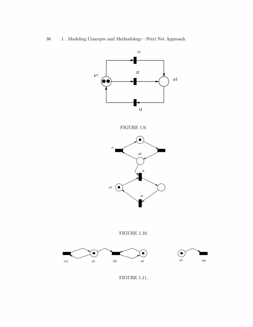
Example 1.10 For the Petri net in fig. 1.9, x1 = (1 0 1)T x2 = (0 1 1)T are

possible minimal-support T-invariants, where kx1k = {t1, t3} and kx2k = {t2, t3}are corresponding minimal supports. All other T-invariants such as x3 = (1 1 2)

T

x4 = (2 1 3)T can be expressed as linear combinations of x1 and x2. That is, x3 =

x1 + x2 and x4 = x21 + x2 . Note that there are many (non-unique) T-invariants

such as x3, x4, etc., corresponding to a nonminimal support {t1, t2, t3}.

One easy way to find T-invariants in an example like this is to simulate all ¨fir-

ing sequence¨which would reproduce a marking, using the concept of ¨negative or

borrowed¨tokens, if necessary.

1.2.4 Simple reduction rules or decomposition techniques

To facilitate the analysis of a large system, we often reduce the system model to a

simpler one, while preserving the system properties to be analyzed. Conversely, tech-

niques to transform an abstracted model into a more refined model in a hierarchical

manner can be used for synthesis.

The following 6 operations preserve the properties of liveness, safeness, and bound-

edness. That is, let (N,M0) and (N0, M 0

0) be the petri nets before and after one of


the following transformations. Then (N 0,M 00) is live, safe, or bounded iff (N,M0) is

live, safe, or bounded, respectively.

1). Fusion of Series Places (FSP) as Fig. (a)

2). Fusion of Series Transitions (FST) as Fig. (b)

3). Fusion of Parallel Places (FPP) as Fig. (c)

4). Fusion of Parallel Transitions (FPT) as Fig. (d)

5). Elimination of Self-loop Places (ESP) as Fig. (e)

6). Elimination of Self-loop Transitions (EST) as Fig. (f)

Example 1.11 The net shown in Fig. 1.10 can be reduced to the one shown in Fig.

1.11 after firing t2 to remove the token in p1 an d then fusing t1 and t2 into t12,

and t3, t4 into t34.

1.3 Abbreviations, extensions and particular structures

1.3.1 classifications

1.3.2 Modeling by Abbreviations

1.3.3 Modeling by Extensions

1.3.4 particular structures (subclasses)


1.4 Summary

• Petri nets are a graphical and mathematical modeling tool applicable to manysystems. They are a promising tool for describing and studying information

processing systems that characterized as being concurrent, asynchronous, dis-

tributed, parallel, non-deterministic, and/or stochastic.

• As a graphical tool, Petri nets can be used as a visual-communication aidsimilar to flow charts, block diagrams, and networks.

• Tokens are used in these nets to simulate the dynamic and concurrent activitiesof systems.

• As a mathematical tool, it is possible to set up state equations, algebraicequations, and other mathematical models governing the behavior of systems.

• Petri nets can be used by both practitioners and theoreticians. Thus, theyprovide a powerful medium of communication between them: practitioners

can learn from theoreticians how to make their models more methodical, and

theoreticians can learn from practitioners how to make their models more

realistic.

1. Colored Petri nets:

Very Brief Introduction to CP-nets

History of Petri Nets

CP-nets at University of Aarhus

Why use CP-nets?

Analysis of CP-nets


Where to Read More about CP-nets

http://www.daimi.aau.dk/CPnets/intro/index.html

2. International Journal on Software Tools for Technology Transfer: Special section

on Coloured Petri Nets

http://sttt.cs.uni-dortmund.de/contents.html

3. Examples of Industrial Use of CP-nets and Design/CPN

http://www.daimi.aau.dk/CPnets/intro/example indu.html


±°²¯

±°²¯

±°²¯±°²¯

±°²¯6

6

±°²¯

±°²¯6

6

?

¾

?

?

?6

?

?

?

6?

-

Comp. CP1requests

Comp. CP1doesn’t need

Comp. CP!uses

Memory freeComp. CP2requests


Comp. CP2uses

±°²¯

±°²¯

±°²¯±°²¯

±°²¯6

6

±°²¯

±°²¯6

6

?

¾

?

?

?6

?

?

?

6?

-

Comp. CP1requests


Comp. CP!uses



Comp. CP2uses

±°²¯

±°²¯

±°²¯±°²¯

±°²¯6

6

±°²¯

±°²¯6

6

?

¾

?

?

?6

?

?

?

6?

-

Comp. CP1requests


Comp. CP!uses



Comp. CP2uses

(a)

(b)

(c)

s s s

ss

s s

sFIGURE 1.3. Third example: twocomputers use a common memory


1p 2p1t

]0,1[1 =m

1p 2p1t

]1,2[2 =m

2 2

FIGURE 1.4. two markings

p1

p2

p3

p4

t1

t2

t3

(a)

p1

p2

p3

p4

t1

t2

t3

(b)

p1

p2

p3

p4

t1

t2

t3

(c)

p1

p2

p3

p4

t1

t2

t3

(d)

FIGURE 1.5. Sequence of transition firings in a petri net


Get 20 c candy

20 c

Deposit5 c

15 c

Get 15 c candy

Deposit5 c

10 c

Deposit5 c

Deposit 10 c5 c

Deposit5 c

Deposit 10 c

Deposit 5 c

0 c

1p

FIGURE 1.6. A Petri net (a state machine) representing the state diagram of a vending

machine, where coin return transitions are omitted.


a

Q

s

B

c

I

a

Q

s

B

c

I

Customer arrives

Customer departs

FIGURE 1.7. Simple queue system and its Petri net model

t2

0

p1

t1

0

t3

0

p3

p2

p4

2

2

2

FIGURE 1.8.


p1p2

t1

t2

t3

FIGURE 1.9.

p2

t1

t3

t4

p3

FIGURE 1.10.

t12 p2 t34 t34p2p3

FIGURE 1.11.


Petri nets

Ordinary PN

abbreviations Finite capacity PN

Generalized PN

Colored PN

extensions

Turing machinesInhibitor arc PN

Priority PN

Continuous and hybrid systems

Continuous PN

Hybrid PN

Non-autonomous PN

Synchronized PN

Timed PN

Interpreted PN

Stochastic PN

Particular structuresMarked graph

State machine

FIGURE 1.12. classification of Petri net models

Discrete Event System Modeling and Simulationdelta.cs.cinvestav.mx/~lixo/Petrinets/notas.pdfThis is...

Documents

Transcript of Discrete Event System Modeling and Simulationdelta.cs.cinvestav.mx/~lixo/Petrinets/notas.pdfThis is...