Discrete Control Barrier Functions forSafety-Critical Control of Discrete Systems with

Application to Bipedal Robot NavigationAuthor Names Omitted for Anonymous Review. Paper-ID 232

Abstract—In this paper, we extend the concept of controlbarrier functions, developed initially for continuous time systems,to the discrete-time domain. We demonstrate safety-critical con-trol for nonlinear discrete-time systems with applications to 3Dbipedal robot navigation. Particularly, we mathematically analyzetwo different formulations of control barrier functions, based ontheir continuous-time counterparts, and demonstrate how thesecan be applied to discrete-time systems. We show that in general,the resulting formulation is a nonlinear program in contrast tothe quadratic program for continuous-time systems. We showthat under certain conditions that the nonlinear program can beformulated as a quadratically constrained quadratic program.Furthermore, using the developed concept of discrete controlbarrier functions, we present a novel control method to addressthe problem of navigation of a high-dimensional bipedal robotthrough environments with moving obstacles that present time-varying safety-critical constraints.

I. INTRODUCTION

Barrier Function based control techniques have recentlygained success in a wide variety continuous-time systems forsafety-critical applications such as precise footstep placementof high degree of freedom bipedal robots [22, 21, 23, 25,26], adaptive cruise control systems [2], multi-agent systems[29, 4] and quadrotor systems [32, 33, 31]. In these, theproblem of stabilization with guaranteed safety is posed asa constrained convex optimization problem, that combinesControl Lyapunov and Control Barrier Functions, and solvesfor an optimal control input that maintains the states of thesystem with a predefined safety set. In [27], Control Barrierand Control Lyapunov Functions are combined through ananalytical framework.

In this paper, we introduce the concept of Control BarrierFunctions (CBFs) to discrete-time dynamical systems. Particu-larly, we analyze the formulation of CBFs presented in [2, 24]and show that these can be applied to directly to discrete-timesystems. Interestingly, however, unlike their continuous-timecounterparts, we find that the resulting optimization problemis not necessarily convex. For the formulation presented in[24], we show that under certain conditions, the optimizationproblem is a Quadratically Constrained Quadratic Program(QCQP).

We then apply these concepts to address the challenge ofbipedal robot navigation in cluttered and dynamically changingenvironments such as in indoor urban spaces with movingobstacles, stairs and narrow passages. An example of such ascenario is presented in Fig. 1. Motion planning for humanoidrobots has been commonly addressed through planning of

Fig. 1: An example scenario of a humanoid robot in a dynam-ically changing environment. We present a navigation schemethat can handle static/moving obstacles (represented by redspheres), while trying to follow a desired path (represented ingreen).

footstep placements in constrained environments to handleobstacles, while operating within kinematic limits of the robot.In [19], a vision-based foot placement method is proposed, andimplemented on the humanoid robot ASIMO, that searchesover a discrete set of actions to avoid obstacles while reachingthe goal. A real-time planning algorithm is presented in[3] that utilizes RRTs to search over dense, pre-computedswept volumes to avoid collision with moving 3D obstacles.Other work related to footstep placement planning include[18, 6, 5, 17]. In [8], a Mixed Integer Convex OptimizationProgram is used to plan footstep placements for bipedal robotwalking on uneven terrains with obstacles. A comprehensivereview of motion planning for humanoid robots, includingwhole body motion planning can be found in [14].

In the context of limit-cycle walkers, footstep placementstrategies based on Barrier Functions to traverse terrains withdiscrete footholds is presented in [21, 23, 25] for 2D robotsand in [22] for high degree of freedom 3D robots. Navigationplanning of 3D dynamic walkers has been studied in [11] andmore recently in [20] by composing asymptotically stable mo-tion primitives. Additionally, [20] provides analytical stabilityguarantees.

In our work, obstacle-free regions are treated as safe sets inthe task space. Discrete-time versions of Control Barrier andControl Lyapunov Functions, developed in this paper, are usedas high-level planners that issue an optimal heading angle atevery to follow a desired path (obtained through path-planningalgorithms like A∗) while simultaneously keeping the robot inthe safe set. A low-level Hybrid Zero Dynamics (HZD) basedcontroller then executes this plan.

The contributions of this paper with respect to prior workare as follows:• We introduce the concept of Control Barrier Functions

[2, 24] for nonlinear discrete-time systems and mathe-matically show the forward invariance of sets associatedwith these Barrier Functions (known as Safety Sets).

• Using the concept of discrete-time Control Barrier Func-tions developed in this paper, we design feedback con-trollers for high degree-of-freedom bipedal robots tofollow a desired path in the task space while avoidingtime-varying unsafe regions such as moving obstacles.

• We evaluate our proposed controller through numericalsimulations for different desired paths and for static andmoving obstacles in the task space.

The rest of the paper is organized as follows. In SectionII, we introduce the concept of Control Lyapunov Functions(CLFs) and Control Barrier Functions (CBFs) for discrete-timedynamical systems and show the invariance of sets associatedwith CBFs. We apply the concept of discrete-time CLFs andCBFs to linear systems show results from numerical simu-lations. In Section III, we apply the concept of ExponentialCBFs developed in [24] to discrete-time systems. Again, weapply this concept to linear systems and show results fromnumerical simulations. In Section IV, we develop an event-based controller for a high dimensional bipedal robot forthe purpose of following a desired path while simultaneouslyavoiding obstacles in the the task space. Finally, in SectionV, we conclude by highlighting certain drawbacks of ourcontroller design and indicating directions for future work.

II. LYAPUNOV AND BARRIER FUNCTIONS FORDISCRETE-TIME SYSTEMS

In this section, we take the concept of Barrier functionsdeveloped for continuous-time systems, particularly in [2, 24]and translate it to discrete-time systems given by:

x(k + 1) = f(x(k)), (1)

where x(k) ∈ D ⊂ Rn represents the state of the system attime step k ∈ Z+ and f : D → D is a continuous function.

Note: Throughout the rest of this paper, we will representthe state of the system x(k) at time step k as xk.

We show that the same formulation of Barrier Functionsdeveloped for continuous-time systems can be applied todiscrete-time systems as well. An important observation fordiscrete-time systems that we will see later is that, unlikecontinuous-time systems, the resulting Lyapunov and Barrierconditions are not necessarily affine in the control input.Rather, they depend on the nature of the system as well as the

nature of the chosen Lyapunov and Barrier Functions them-selves. Implementing Control Lyapunov and Control BarrierFunctions through optimization may then turn into a poten-tially non-convex nonlinear program. For the formulation ofCBFs in [24], we show that the resulting optimization problemis convex for a class of nonlinear systems and CLFs/CBFs.

A. Lyapunov Functions for Discrete-Time Systems

Consider the nonlinear discrete-time control system,

xk+1 = f (xk, uk) , (2)

where uk ∈ U ⊂ Rm is the control input at time step k andU is the set of admissible control inputs.

Definition 1. (Discrete-Time Exponentially stabilizing Con-trol Lyapunov Function): A map V : D → R is an Exponen-tial Control Lyapunov Function for the discrete-time controlsystem (2) if there exists:

1) positive constants c1 and c2 such that

c1‖xk‖2 ≤ V (xk) ≤ c2‖xk‖2, (3)

and2) a control input uk : D → U, ∀xk ∈ D and c3 > 0 such

that

∆V (xk, uk) + c3‖xk‖2 ≤ 0, (4)

where,

∆V (xk, uk) := V (xk+1)− V (xk)

= ∆Vk.

Remark 1. The control input uk renders the origin exponen-tially stable. See [16] for a comprehensive stability analysisfor discrete-time systems.

The concept of Discrete-Time Control Lyapunov Functionshas been previously studied in [13] and applied to an automo-tive engine control problem.

Similar to [9] for continuous-time systems, the CLF con-dition (4) can be enforced through a constrained optimizationprogram:

u∗k = argminuk

uTk uk

uk ∈ Rm

s.t. ∆V (xk, uk) + c3‖xk‖2 ≤ 0.

(5)

B. Barrier Functions for Discrete-Time Systems

We now show the forward invariance of a set S, know asthe Safety Set,

S := {x(k) ∈ D | h(x(k)) ≥ 0}, (6)∂S := {x(k) ∈ D | h(x(k)) = 0}, (7)

for a smooth function h : Rn → R associated with a Barrierfunction defined similar to [2] as,

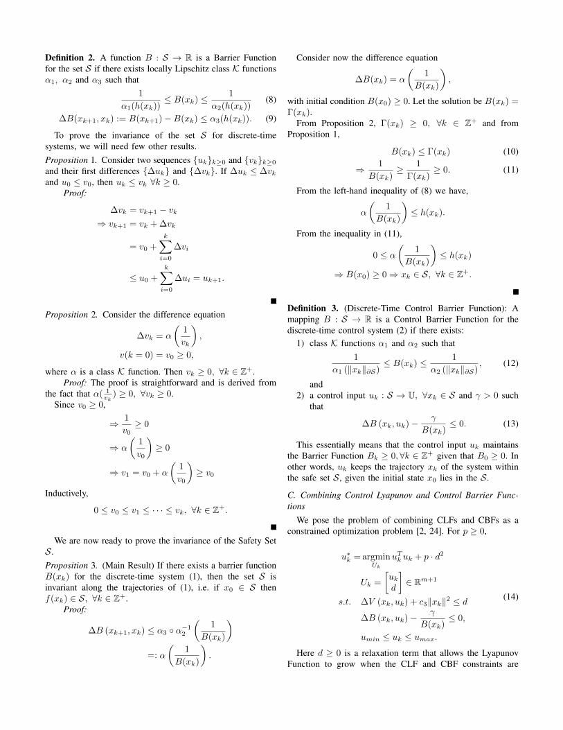
Definition 2. A function B : S → R is a Barrier Functionfor the set S if there exists locally Lipschitz class K functionsα1, α2 and α3 such that

1

α1(h(xk))≤ B(xk) ≤ 1

α2(h(xk))(8)

∆B(xk+1, xk) := B(xk+1)−B(xk) ≤ α3(h(xk)). (9)

To prove the invariance of the set S for discrete-timesystems, we will need few other results.Proposition 1. Consider two sequences {uk}k≥0 and {vk}k≥0

and their first differences {∆uk} and {∆vk}. If ∆uk ≤ ∆vkand u0 ≤ v0, then uk ≤ vk ∀k ≥ 0.

Proof:

∆vk = vk+1 − vk⇒ vk+1 = vk + ∆vk

= v0 +

k∑i=0

∆vi

≤ u0 +

k∑i=0

∆ui = uk+1.

Proposition 2. Consider the difference equation

∆vk = α

(1

vk

),

v(k = 0) = v0 ≥ 0,

where α is a class K function. Then vk ≥ 0, ∀k ∈ Z+.Proof: The proof is straightforward and is derived from

the fact that α( 1vk

) ≥ 0, ∀vk ≥ 0.Since v0 ≥ 0,

⇒ 1

v0≥ 0

⇒ α

(1

v0

)≥ 0

⇒ v1 = v0 + α

(1

v0

)≥ v0

Inductively,

0 ≤ v0 ≤ v1 ≤ · · · ≤ vk, ∀k ∈ Z+.

We are now ready to prove the invariance of the Safety SetS .Proposition 3. (Main Result) If there exists a barrier functionB(xk) for the discrete-time system (1), then the set S isinvariant along the trajectories of (1), i.e. if x0 ∈ S thenf(xk) ∈ S, ∀k ∈ Z+.

Proof:

∆B (xk+1, xk) ≤ α3 ◦ α−12

(1

B(xk)

)=: α

(1

B(xk)

).

Consider now the difference equation

∆B(xk) = α

(1

B(xk)

),

with initial condition B(x0) ≥ 0. Let the solution be B(xk) =Γ(xk).

From Proposition 2, Γ(xk) ≥ 0, ∀k ∈ Z+ and fromProposition 1,

B(xk) ≤ Γ(xk) (10)

⇒ 1

B(xk)≥ 1

Γ(xk)≥ 0. (11)

From the left-hand inequality of (8) we have,

α

(1

B(xk)

)≤ h(xk).

From the inequality in (11),

0 ≤ α(

1

B(xk)

)≤ h(xk)

⇒ B(x0) ≥ 0⇒ xk ∈ S, ∀k ∈ Z+.

Definition 3. (Discrete-Time Control Barrier Function): Amapping B : S → R is a Control Barrier Function for thediscrete-time control system (2) if there exists:

1) class K functions α1 and α2 such that1

α1 (‖xk‖∂S)≤ B(xk) ≤ 1

α2 (‖xk‖∂S), (12)

and2) a control input uk : S → U, ∀xk ∈ S and γ > 0 such

that

∆B (xk, uk)− γ

B(xk)≤ 0. (13)

This essentially means that the control input uk maintainsthe Barrier Function Bk ≥ 0,∀k ∈ Z+ given that B0 ≥ 0. Inother words, uk keeps the trajectory xk of the system withinthe safe set S, given the initial state x0 lies in the S.

C. Combining Control Lyapunov and Control Barrier Func-tions

We pose the problem of combining CLFs and CBFs as aconstrained optimization problem [2, 24]. For p ≥ 0,

u∗k = argminUk

uTk uk + p · d2

Uk =

[ukd

]∈ Rm+1

s.t. ∆V (xk, uk) + c3‖xk‖2 ≤ d

∆B (xk, uk)− γ

B(xk)≤ 0,

umin ≤ uk ≤ umax.

(14)

Here d ≥ 0 is a relaxation term that allows the LyapunovFunction to grow when the CLF and CBF constraints are

conflicting. Note that the CBF condition is always satisfiedand the trajectory of the system x(k) always remains withinthe safe set S. umin and umax are bounds on the control input.Remark 2. Here, we assume that the optimization problem in(14) is always feasible.

D. Application to Linear Systems

Consider the discrete-time linear system,

xk+1 = Axk +Duk, (15)

with xk ∈ Rn, uk ∈ Rm, A ∈ Rn×n, D ∈ Rn×m and the safeset S defined by the linear function

h(xk) = Hxk + F, (16)

with H ∈ R1×n and F ∈ R. We choose a quadratic ControlLyapunov Function

Vk = xTk Pxk,

with P > 0 and symmetric, obtained by solving the discrete-time Lyapunov equation,

ATPA− P = −Q

for a positive definite and symmetric matrix Q. The CLFcondition (4) is then given by:

∆Vk + c3‖xk‖2 = Vk+1 − Vk + c3xTk xk

= xTk+1Pxk+1 − xTk Pxk + c3xTk xk

= uTkDTPDuk + xTk (ATPA− P )xk+

2xTkAPDuk + c3xTk xk ≤ 0

Similar to the continuous-time domain [2], we chose thefollowing Control Barrier Function,

Bk = B(xk) =1

h(xk)

= (Hxk + F )−1.

The CBF condition (13) then becomes

∆Bk −γ

Bk= Bk+1 −Bk −

γ

Bk

= − H(Axk − xk +Duk)

(HAxk +HDuk + F )(Hxk + F )

− γ(Hxk + F )

≤ 0

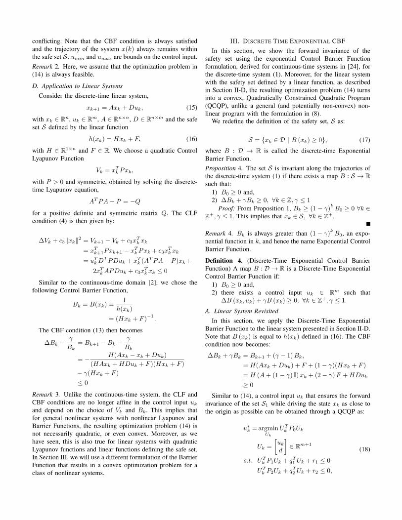
Remark 3. Unlike the continuous-time system, the CLF andCBF conditions are no longer affine in the control input ukand depend on the choice of Vk and Bk. This implies thatfor general nonlinear systems with nonlinear Lyapunov andBarrier Functions, the resulting optimization problem (14) isnot necessarily quadratic, or even convex. Moreover, as wehave seen, this is also true for linear systems with quadraticLyapunov functions and linear functions defining the safe set.In Section III, we will use a different formulation of the BarrierFunction that results in a convex optimization problem for aclass of nonlinear systems.

III. DISCRETE TIME EXPONENTIAL CBFIn this section, we show the forward invariance of the

safety set using the exponential Control Barrier Functionformulation, derived for continuous-time systems in [24], forthe discrete-time system (1). Moreover, for the linear systemwith the safety set defined by a linear function, as describedin Section II-D, the resulting optimization problem (14) turnsinto a convex, Quadratically Constrained Quadratic Program(QCQP), unlike a general (and potentially non-convex) non-linear program with the formulation in (8).

We redefine the definition of the safety set, S as:

S = {xk ∈ D | B (xk) ≥ 0}, (17)

where B : D → R is called the discrete-time ExponentialBarrier Function.Proposition 4. The set S is invariant along the trajectories ofthe discrete-time system (1) if there exists a map B : S → Rsuch that:

1) B0 ≥ 0 and,2) ∆Bk + γBk ≥ 0, ∀k ∈ Z, γ ≤ 1

Proof: From Proposition 1, Bk ≥ (1− γ)kB0 ≥ 0 ∀k ∈

Z+, γ ≤ 1. This implies that xk ∈ S, ∀k ∈ Z+.

Remark 4. Bk is always greater than (1− γ)kB0, an expo-

nential function in k, and hence the name Exponential ControlBarrier Function.

Definition 4. (Discrete-Time Exponential Control BarrierFunction) A map B : D → R is a Discrete-Time ExponentialControl Barrier Function if:

1) B0 ≥ 0 and,2) there exists a control input uk ∈ Rm such that

∆B (xk, uk) + γB (xk) ≥ 0, ∀k ∈ Z+, γ ≤ 1.

A. Linear System RevisitedIn this section, we apply the Discrete-Time Exponential

Barrier Function to the linear system presented in Section II-D.Note that B (xk) is equal to h(xk) defined in (16). The CBFcondition now becomes:

∆Bk + γBk = Bk+1 + (γ − 1)Bk,

= H(Axk +Duk) + F + (1− γ)(Hxk + F )

= H (A+ (1− γ) I)xk + (2− γ)F +HDuk

≥ 0

Similar to (14), a control input uk that ensures the forwardinvariance of the set S1 while driving the state xk as close tothe origin as possible can be obtained through a QCQP as:

u∗k = argminUk

UTk P0Uk

Uk =

[ukd

]∈ Rm+1

s.t. UTk P1Uk + qT1 Uk + r1 ≤ 0

UTk P2Uk + qT2 Uk + r2 ≤ 0,

(18)

where,

P0 =

[Im×m

p

]P1 =

[DTPD

0

]P2 = 0m×m

q1 =[2xTkAPD −1

]Tq2 =

[−HD 0

]Tr1 = xTk (ATPA− P + c3In×n)xk

r2 = −H (A+ (1− γ) I)xk − (2− γ)F.

Remark 5. As we have seen here, the exponential CBF formu-lation results in a convex optimization problem (particularlya QCQP) for a linear system with quadratic Lyapunov andBarrier functions. Moreover, this is also true for nonlinear,control affine systems with Linear and/or Quadratic Lyapunovand Barrier functions. This can be solved efficiently usingMATLAB’s fmincon [1] using packages such as CVX [10].

B. Example

We now present simple examples of the discrete-time CBF-CLF controllers for both linear and nonlinear control affinesystems.

Consider the linear system with A, D, H and F matricesgiven by,

A =

[1 22 2

],

B =[1 2

]T,

H =[1 0

],

F = −1.5.

(19)

Utilizing the discrete-time CBF-CLF controller in (14), thetrajectory of the system always remains within the safer region(see Fig.2a).

Consider now the discrete-time control affine nonlinearsystem given by,

[xk+1,1

xk+1,2

]=

[sin (xk,1) + xk,1 + 2xk,2 + uksin (xk,2) + 2xk,1 + 2xk,2 + 2uk

]. (20)

Linearizing the above nonlinear system yields the linearsystem in (19).

Like in the case of the linear system, the trajectories of thenonlinear system in (20) also the remain within the safety set(See Fig.2b).

IV. APPLICATION TO BIPEDAL WALKING

In this section, we use the concept of Discrete-Time ControlLyapunov (D-CLF) and Barrier Functions (D-CBF) to developa stride-to-stride controller for a 21 degree of freedom bipedalrobot model to follow a given path in the task space, whileavoiding static and moving obstacles. We begin by presentinga brief overview of the hybrid zero dynamics framework

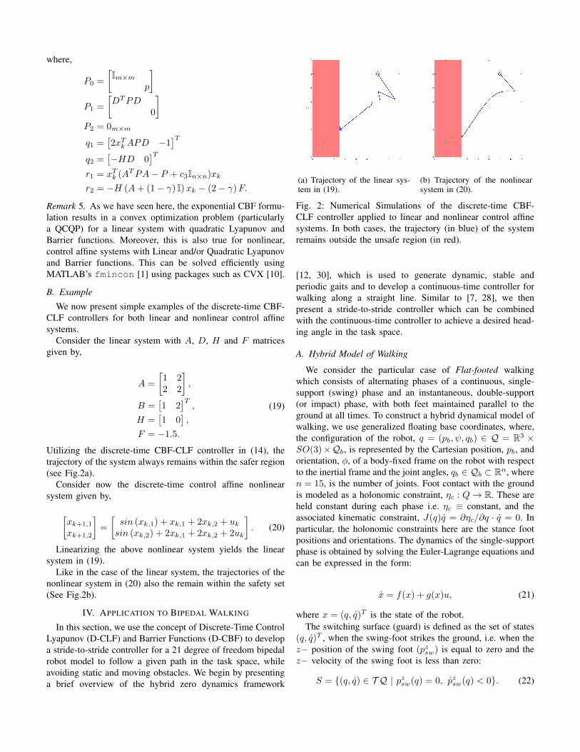
(a) Trajectory of the linear sys-tem in (19).

(b) Trajectory of the nonlinearsystem in (20).

Fig. 2: Numerical Simulations of the discrete-time CBF-CLF controller applied to linear and nonlinear control affinesystems. In both cases, the trajectory (in blue) of the systemremains outside the unsafe region (in red).

[12, 30], which is used to generate dynamic, stable andperiodic gaits and to develop a continuous-time controller forwalking along a straight line. Similar to [7, 28], we thenpresent a stride-to-stride controller which can be combinedwith the continuous-time controller to achieve a desired head-ing angle in the task space.

A. Hybrid Model of Walking

We consider the particular case of Flat-footed walkingwhich consists of alternating phases of a continuous, single-support (swing) phase and an instantaneous, double-support(or impact) phase, with both feet maintained parallel to theground at all times. To construct a hybrid dynamical model ofwalking, we use generalized floating base coordinates, where,the configuration of the robot, q = (pb, ψ, qb) ∈ Q = R3 ×SO(3)×Qb, is represented by the Cartesian position, pb, andorientation, φ, of a body-fixed frame on the robot with respectto the inertial frame and the joint angles, qb ∈ Qb ⊂ Rn, wheren = 15, is the number of joints. Foot contact with the groundis modeled as a holonomic constraint, ηc : Q→ R. These areheld constant during each phase i.e. ηc ≡ constant, and theassociated kinematic constraint, J(q)q = ∂ηc/∂q · q = 0. Inparticular, the holonomic constraints here are the stance footpositions and orientations. The dynamics of the single-supportphase is obtained by solving the Euler-Lagrange equations andcan be expressed in the form:

x = f(x) + g(x)u, (21)

where x = (q, q)T is the state of the robot.The switching surface (guard) is defined as the set of states

(q, q)T , when the swing-foot strikes the ground, i.e. when thez− position of the swing foot (pzsw) is equal to zero and thez− velocity of the swing foot is less than zero:

S = {(q, q) ∈ T Q | pzsw(q) = 0, pzsw(q) < 0}. (22)

This is when the transition from single support to doublesupport phase occurs. At impact, there is a discrete change inthe velocities of the robot, while the configurations remain thesame. The post impact states, (q+, q+) are determined from theimpact map ∆ (q−, q−), given the pre-impact states, (q−, q−),assuming a perfectly plastic impact. The hybrid model of thesystem is then comprised of the continuous time dynamics andthe discrete dynamics:

Σ :

{x = f(x) + g(x)u, x /∈ S,x+ = ∆(x−), x ∈ S.

(23)

We define the set,

N := {(q, q) ∈ T Q | ηc = ηc(q+), J(q)q = 0},

as the set of states such that the holonomic constraints aresatisfied.

B. Hybrid Zero Dynamics (HZD) Control

a) Virtual Constraints: We define a set of outputs (alsoreferred to as virtual constraints), y ∈ Rm, for the controlsystem (23), which consists of velocity regulating and positionmodulating terms. These are defined as the difference betweenthe actual output, ya(x) and desired output, yd(τ, α),

y := ya(x)− yd(τ, α),

where τ(q) ∈ [0, 1] is the gait phasing variable and α ∈Rm×(b+1) is a set of Bezier Polynomial coefficients of degreeb that parametrize the desired position modulating outputs.An input-output linearizing controller ΓIO drives y → 0exponentially [30].

A stable and periodic walking gait can be designed bychoosing appropriate values for the parameters, α, that ensurea periodic solution exists for the hybrid system in (23) andthe Partial Hybrid Zero Dynamics surface [15] is impactinvariant. This can be posed as a nonlinear, constrainedoptimization problem. Additionally, physical constraints suchas joint velocity limits and actuator input bounds, as well as,robot behaviors such as desired step length and walking speedcan be incorporated in this optimization problem. Specifically,we utilize the direct collocation framework presented in [15].Figure. 3 shows snapshots of a step of the walking gaitobtained using this optimization process.

Fig. 3: Snapshots of a single step of walking obtained usingthe the direct collocation optimization method.

C. Stride-to-Stride Controller for Turning

The input-output linearizing controller can be combinedwith a discrete-time controller based on the Poincare map,similar to [28, 7, 20], to follow a desired heading angle, φ.Specifically, we define the Poincare map P : N ∩∆(S)×B 7→N ∩∆(S)× B as:

xk+1 := P (xk, βk), (24)

where xk ∈ N ∩∆(S) ⊂ R(2n−nc+11), is the reduced set ofstates on the post impact surface, ∆(S), and which satisfy theholonomic constraints, at the kth step. βk ∈ B ⊂ Rm is a setof parameters that modifies the outputs, y, towards the end ofa step,

y = ya(q, q)− yd(τ, α)− yb(τ, βk) (25)

with yb defined as,yb = 0 if τ = 0

yb = βk if τ = 1∂yb

∂τ = 0 if τ = {0, 1}

The linearized Poincare map,

δxk+1 = Aδxk + Bδβk, (26)

can be treated a discrete-time control system, where δxk :=xk−x∗ and δβk = βk−β∗, with x∗ a fixed point of (24) andβ∗ = 0m×1. A and B are the Jacobians of P with respect to xrand β respectively. A feedback controller Γβ : N∩∆(S)→ B,

δβk = Γβ = −Kδ ·(xk − xd

(∆φdk

)), (27)

with Kδ obtained using the DLQR method and xd being x∗

with the heading angle replaced by the desired change inheading angle ∆φdk, can be developed such that the eigenvaluesof (A− BKδ) are within the unit circle.

Fig. 4a shows the path traversed by the robot for differentdesired heading angles while Fig. 4b shows snapshots of therobot for walking on a circular path, both using the event-basedcontroller (27).

D. Path Following

Using the above controller, we can follow a desired pathby changing the heading angle of the robot from step to step.Consider the desired path can be represented by,

pdy = ζ (px) , (28)

where pdy is the desired vertical position of the robot, px isthe current horizontal position of the robot and ζ : R→ R isa smooth function.Remark 6. A desired path for the robot’s position can becomputed offline from existing path planning algorithms suchas RRTs or A∗ search.

From (26) and (27), another system can be constructed,

pstk+1 (xk+1) = P(pstk (xk) ,∆φdk

), (29)

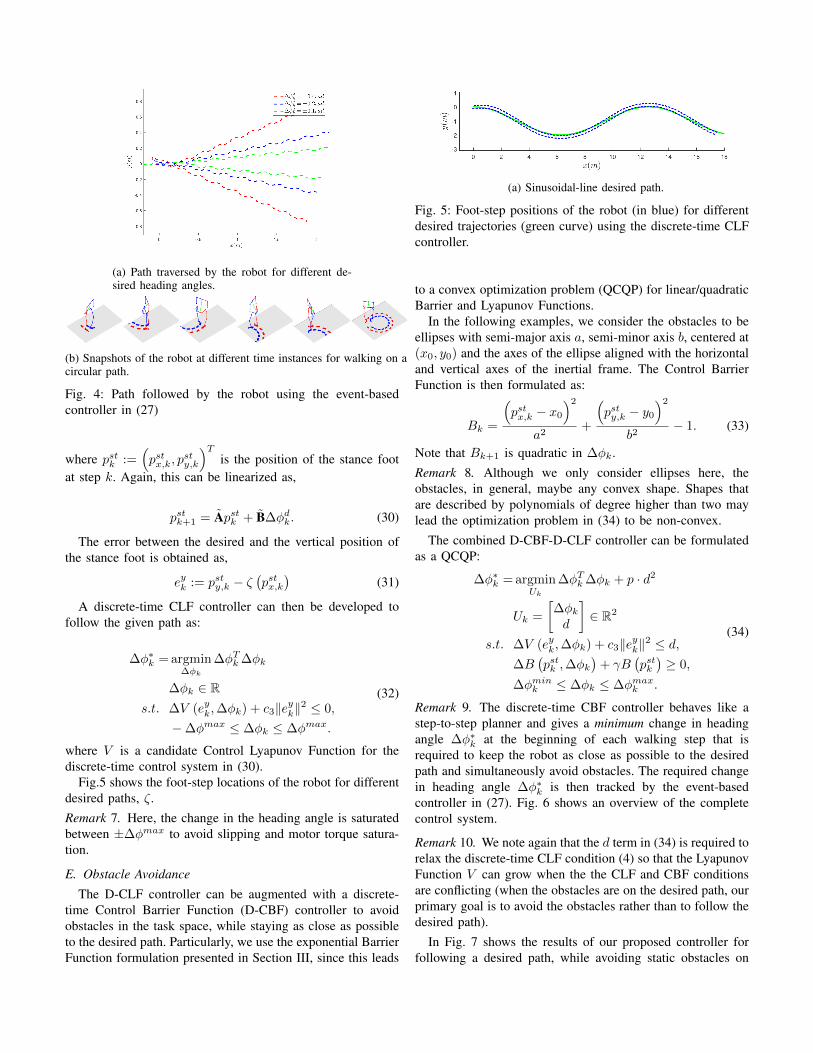
(a) Path traversed by the robot for different de-sired heading angles.

(b) Snapshots of the robot at different time instances for walking on acircular path.

Fig. 4: Path followed by the robot using the event-basedcontroller in (27)

where pstk :=(pstx,k, p

sty,k

)Tis the position of the stance foot

at step k. Again, this can be linearized as,

pstk+1 = Apstk + B∆φdk. (30)

The error between the desired and the vertical position ofthe stance foot is obtained as,

eyk := psty,k − ζ(pstx,k

)(31)

A discrete-time CLF controller can then be developed tofollow the given path as:

∆φ∗k = argmin∆φk

∆φTk ∆φk

∆φk ∈ Rs.t. ∆V (eyk,∆φk) + c3‖eyk‖

2 ≤ 0,

−∆φmax ≤ ∆φk ≤ ∆φmax.

(32)

where V is a candidate Control Lyapunov Function for thediscrete-time control system in (30).

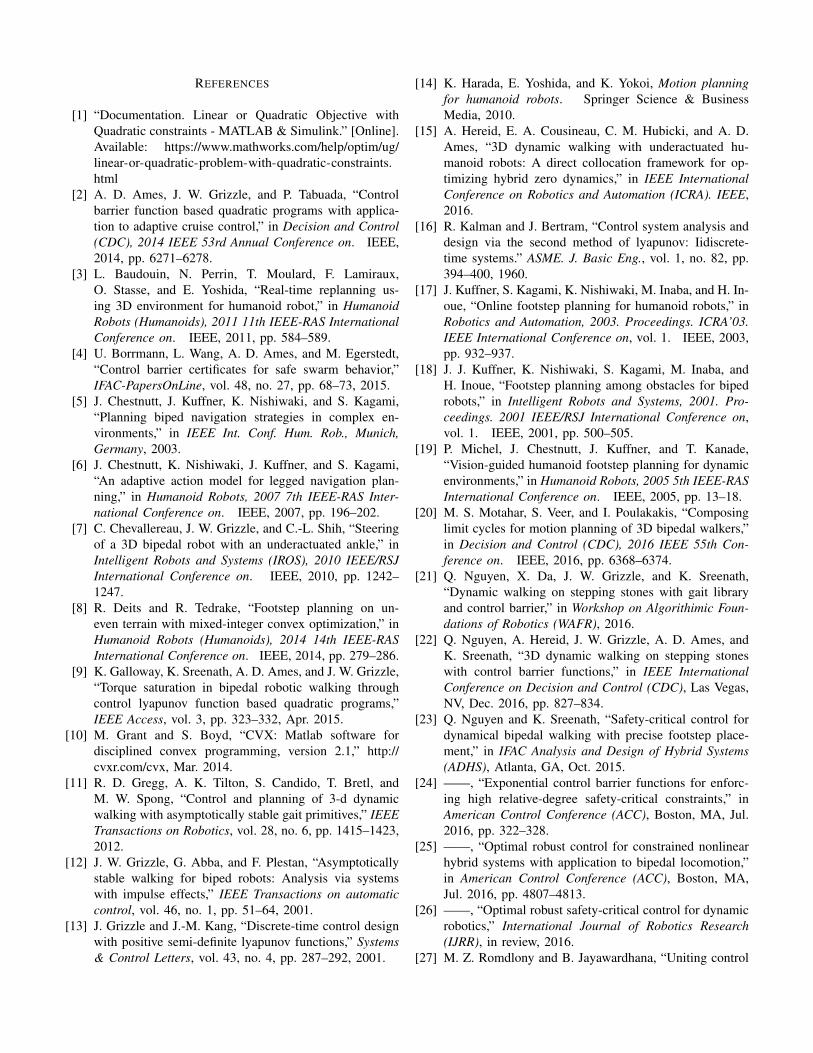
Fig.5 shows the foot-step locations of the robot for differentdesired paths, ζ.Remark 7. Here, the change in the heading angle is saturatedbetween ±∆φmax to avoid slipping and motor torque satura-tion.

E. Obstacle Avoidance

The D-CLF controller can be augmented with a discrete-time Control Barrier Function (D-CBF) controller to avoidobstacles in the task space, while staying as close as possibleto the desired path. Particularly, we use the exponential BarrierFunction formulation presented in Section III, since this leads

(a) Sinusoidal-line desired path.

Fig. 5: Foot-step positions of the robot (in blue) for differentdesired trajectories (green curve) using the discrete-time CLFcontroller.

to a convex optimization problem (QCQP) for linear/quadraticBarrier and Lyapunov Functions.

In the following examples, we consider the obstacles to beellipses with semi-major axis a, semi-minor axis b, centered at(x0, y0) and the axes of the ellipse aligned with the horizontaland vertical axes of the inertial frame. The Control BarrierFunction is then formulated as:

Bk =

(pstx,k − x0

)2

a2+

(psty,k − y0

)2

b2− 1. (33)

Note that Bk+1 is quadratic in ∆φk.Remark 8. Although we only consider ellipses here, theobstacles, in general, maybe any convex shape. Shapes thatare described by polynomials of degree higher than two maylead the optimization problem in (34) to be non-convex.

The combined D-CBF-D-CLF controller can be formulatedas a QCQP:

∆φ∗k = argminUk

∆φTk ∆φk + p · d2

Uk =

[∆φkd

]∈ R2

s.t. ∆V (eyk,∆φk) + c3‖eyk‖2 ≤ d,

∆B(pstk ,∆φk

)+ γB

(pstk)≥ 0,

∆φmink ≤ ∆φk ≤ ∆φmaxk .

(34)

Remark 9. The discrete-time CBF controller behaves like astep-to-step planner and gives a minimum change in headingangle ∆φ∗k at the beginning of each walking step that isrequired to keep the robot as close as possible to the desiredpath and simultaneously avoid obstacles. The required changein heading angle ∆φ∗k is then tracked by the event-basedcontroller in (27). Fig. 6 shows an overview of the completecontrol system.

Remark 10. We note again that the d term in (34) is required torelax the discrete-time CLF condition (4) so that the LyapunovFunction V can grow when the the CLF and CBF conditionsare conflicting (when the obstacles are on the desired path, ourprimary goal is to avoid the obstacles rather than to follow thedesired path).

In Fig. 7 shows the results of our proposed controller forfollowing a desired path, while avoiding static obstacles on

Fig. 6: Overview of the proposed controller. Dashed linesrepresent signals in discrete-time

(a) Straight-line desired path.

(b) Sinusoidal desired path.

Fig. 7: Foot-step positions of the robot (in blue) for differentdesired trajectories (green curve) while avoiding static obsta-cles (red circle) using the discrete-time CBF-CLF controller.

it. Fig. 8 shows snapshots of the robot’s foot position for thecase with moving obstacles.Remark 11. For the case of moving obstacles, we assume thatthe robot does not strike any obstacles during the swing phase.This is a reasonable assumption since the step times are in theorder of 1s.Remark 12. For the case of avoiding moving obstacles,traditional path-planning algorithms such as RRTs could bepotentially inefficient.Remark 13. The discrete time CBF-CLF controller (34) canbe concatenated with a continuous-time CBF-CLF controller[9, 21, 25] to traverse over more complex terrains such asstepping stones while avoiding obstacles.

V. CONCLUSION

In this paper, we took tools recently developed for safety-critical applications of continuous-time systems and showedmathematically how they can be extended to discrete-time sys-tems. For discrete-time systems, however, using the definitionof Barrier Functions in (8) and (9) an additional complexityarises in that the resulting optimization problem to solve forthe optimal control input is not necessarily convex. We thenused the concept of Exponential Control Barrier Functions andshowed that for nonlinear control-affine discrete-time systems,

Fig. 8: Snapshots of the robot’s stance foot (in blue) at differentsteps, k. Red circle represents moving obstacle, green linerepresents the desired trajectory.

the CLF and CBF conditions are quadratic for quadraticLyapunov and linear barrier functions and the resulting op-timization problem is a convex, a Quadratically ConstrainedQuadratic Program.

Using this concept of CLFs and CBFs for discrete-timesystems, we then developed a stride-to-stride controller forpath-following and obstacle avoidance in the task space for ahigh-dimensional bipedal robot.

In our control design however, we do make certain simpli-fications and assumptions, which include a linearized modelsfor the Poincare Map (26) and foot-step placement (30), whichresults in a slightly inaccurate estimate of footstep position.This can be addressed by formulating enlarged barriers, equiv-alent to the amount of uncertainty in estimating the footsteppositions. We also assume that we have knowledge about thefull state of the robot (such as its position in the inertial frame)and the environment (such as position of obstacles with respectto the robot). In future work, we intend to address this byintegrating vision sensors in our control design to estimate thelocation of obstacles. A primary advantage of bipedal robots isto step over obstacles (of reasonable size) and uneven terrain.In this work, however, we do not consider this. We seek toaddress this in future by integrating the discrete-time CBFcontroller with the continuous-time controllers presented in[21, 24, 23, 25] to achieve more complex tasks such as walk-ing over discrete footholds or avoiding overhead obstacles.Another important assumption we make is the feasibility ofthe optimization problem in (14) to guarantee invariance ofthe safe set.

REFERENCES

[1] “Documentation. Linear or Quadratic Objective withQuadratic constraints - MATLAB & Simulink.” [Online].Available: https://www.mathworks.com/help/optim/ug/linear-or-quadratic-problem-with-quadratic-constraints.html

[2] A. D. Ames, J. W. Grizzle, and P. Tabuada, “Controlbarrier function based quadratic programs with applica-tion to adaptive cruise control,” in Decision and Control(CDC), 2014 IEEE 53rd Annual Conference on. IEEE,2014, pp. 6271–6278.

[3] L. Baudouin, N. Perrin, T. Moulard, F. Lamiraux,O. Stasse, and E. Yoshida, “Real-time replanning us-ing 3D environment for humanoid robot,” in HumanoidRobots (Humanoids), 2011 11th IEEE-RAS InternationalConference on. IEEE, 2011, pp. 584–589.

[4] U. Borrmann, L. Wang, A. D. Ames, and M. Egerstedt,“Control barrier certificates for safe swarm behavior,”IFAC-PapersOnLine, vol. 48, no. 27, pp. 68–73, 2015.

[5] J. Chestnutt, J. Kuffner, K. Nishiwaki, and S. Kagami,“Planning biped navigation strategies in complex en-vironments,” in IEEE Int. Conf. Hum. Rob., Munich,Germany, 2003.

[6] J. Chestnutt, K. Nishiwaki, J. Kuffner, and S. Kagami,“An adaptive action model for legged navigation plan-ning,” in Humanoid Robots, 2007 7th IEEE-RAS Inter-national Conference on. IEEE, 2007, pp. 196–202.

[7] C. Chevallereau, J. W. Grizzle, and C.-L. Shih, “Steeringof a 3D bipedal robot with an underactuated ankle,” inIntelligent Robots and Systems (IROS), 2010 IEEE/RSJInternational Conference on. IEEE, 2010, pp. 1242–1247.

[8] R. Deits and R. Tedrake, “Footstep planning on un-even terrain with mixed-integer convex optimization,” inHumanoid Robots (Humanoids), 2014 14th IEEE-RASInternational Conference on. IEEE, 2014, pp. 279–286.

[9] K. Galloway, K. Sreenath, A. D. Ames, and J. W. Grizzle,“Torque saturation in bipedal robotic walking throughcontrol lyapunov function based quadratic programs,”IEEE Access, vol. 3, pp. 323–332, Apr. 2015.

[10] M. Grant and S. Boyd, “CVX: Matlab software fordisciplined convex programming, version 2.1,” http://cvxr.com/cvx, Mar. 2014.

[11] R. D. Gregg, A. K. Tilton, S. Candido, T. Bretl, andM. W. Spong, “Control and planning of 3-d dynamicwalking with asymptotically stable gait primitives,” IEEETransactions on Robotics, vol. 28, no. 6, pp. 1415–1423,2012.

[12] J. W. Grizzle, G. Abba, and F. Plestan, “Asymptoticallystable walking for biped robots: Analysis via systemswith impulse effects,” IEEE Transactions on automaticcontrol, vol. 46, no. 1, pp. 51–64, 2001.

[13] J. Grizzle and J.-M. Kang, “Discrete-time control designwith positive semi-definite lyapunov functions,” Systems& Control Letters, vol. 43, no. 4, pp. 287–292, 2001.

[14] K. Harada, E. Yoshida, and K. Yokoi, Motion planningfor humanoid robots. Springer Science & BusinessMedia, 2010.

[15] A. Hereid, E. A. Cousineau, C. M. Hubicki, and A. D.Ames, “3D dynamic walking with underactuated hu-manoid robots: A direct collocation framework for op-timizing hybrid zero dynamics,” in IEEE InternationalConference on Robotics and Automation (ICRA). IEEE,2016.

[16] R. Kalman and J. Bertram, “Control system analysis anddesign via the second method of lyapunov: Iidiscrete-time systems.” ASME. J. Basic Eng., vol. 1, no. 82, pp.394–400, 1960.

[17] J. Kuffner, S. Kagami, K. Nishiwaki, M. Inaba, and H. In-oue, “Online footstep planning for humanoid robots,” inRobotics and Automation, 2003. Proceedings. ICRA’03.IEEE International Conference on, vol. 1. IEEE, 2003,pp. 932–937.

[18] J. J. Kuffner, K. Nishiwaki, S. Kagami, M. Inaba, andH. Inoue, “Footstep planning among obstacles for bipedrobots,” in Intelligent Robots and Systems, 2001. Pro-ceedings. 2001 IEEE/RSJ International Conference on,vol. 1. IEEE, 2001, pp. 500–505.

[19] P. Michel, J. Chestnutt, J. Kuffner, and T. Kanade,“Vision-guided humanoid footstep planning for dynamicenvironments,” in Humanoid Robots, 2005 5th IEEE-RASInternational Conference on. IEEE, 2005, pp. 13–18.

[20] M. S. Motahar, S. Veer, and I. Poulakakis, “Composinglimit cycles for motion planning of 3D bipedal walkers,”in Decision and Control (CDC), 2016 IEEE 55th Con-ference on. IEEE, 2016, pp. 6368–6374.

[21] Q. Nguyen, X. Da, J. W. Grizzle, and K. Sreenath,“Dynamic walking on stepping stones with gait libraryand control barrier,” in Workshop on Algorithimic Foun-dations of Robotics (WAFR), 2016.

[22] Q. Nguyen, A. Hereid, J. W. Grizzle, A. D. Ames, andK. Sreenath, “3D dynamic walking on stepping stoneswith control barrier functions,” in IEEE InternationalConference on Decision and Control (CDC), Las Vegas,NV, Dec. 2016, pp. 827–834.

[23] Q. Nguyen and K. Sreenath, “Safety-critical control fordynamical bipedal walking with precise footstep place-ment,” in IFAC Analysis and Design of Hybrid Systems(ADHS), Atlanta, GA, Oct. 2015.

[24] ——, “Exponential control barrier functions for enforc-ing high relative-degree safety-critical constraints,” inAmerican Control Conference (ACC), Boston, MA, Jul.2016, pp. 322–328.

[25] ——, “Optimal robust control for constrained nonlinearhybrid systems with application to bipedal locomotion,”in American Control Conference (ACC), Boston, MA,Jul. 2016, pp. 4807–4813.

[26] ——, “Optimal robust safety-critical control for dynamicrobotics,” International Journal of Robotics Research(IJRR), in review, 2016.

[27] M. Z. Romdlony and B. Jayawardhana, “Uniting control

lyapunov and control barrier functions,” in Decision andControl (CDC), 2014 IEEE 53rd Annual Conference on.IEEE, 2014, pp. 2293–2298.

[28] C.-L. Shih, J. Grizzle, and C. Chevallereau, “From stablewalking to steering of a 3D bipedal robot with passivepoint feet,” Robotica, vol. 30, no. 07, pp. 1119–1130,2012.

[29] L. Wang, A. Ames, and M. Egerstedt, “Safety barriercertificates for heterogeneous multi-robot systems,” inAmerican Control Conference (ACC), 2016. IEEE, 2016,pp. 5213–5218.

[30] E. R. Westervelt, J. W. Grizzle, C. Chevallereau, J. H.Choi, and B. Morris, Feedback control of dynamicbipedal robot locomotion. CRC press, 2007, vol. 28.

[31] G. Wu and K. Sreenath, “Safety-critical control of a 3Dquadrotor with range-limited sensing,” in ASME Dynam-ics Systems and Control Conference (DSCC), Minneapo-lis, MN, Oct. 2016.

[32] ——, “Safety-critical control of a planar quadrotor,” inAmerican Control Conference (ACC), Boston, MA, Jul.2016, pp. 2252–2258.

[33] ——, “Safety-critical geometric control for systems onmanifolds subject to time-varying constraints,” IEEETransactions on Automatic Control (TAC), in review,2016.