Discover 3D 2013 Tutorials - Pitney...
74
Pitney Bowes Software Inc. is a wholly-owned subsidiary of Pitney Bowes Inc. Pitney Bowes, the Corporate logo, pbEncom and Discover are [registered] trademarks of Pitney Bowes Inc. or a subsidiary. All other trademarks are the property of their respective owners. © 2013 Pitney Bowes Software Inc. All rights reserved. Discover TM 3D 2013 Tutorials
Transcript of Discover 3D 2013 Tutorials - Pitney...

Pitney Bowes Software Inc. is a wholly-owned subsidiary of Pitney Bowes Inc. Pitney Bowes, the Corporate logo, pbEncom and Discover are [registered] trademarks of Pitney Bowes Inc. or a subsidiary. All other trademarks are the property of their respective owners. © 2013 Pitney Bowes Software Inc. All rights reserved.
DiscoverTM 3D 2013 Tutorials

Table of Contents
1 Introduction ................................................................................................ 1
2 Display 3D Surface and Draped Images ................................................... 5
3 Drape Vectors Over Surface ................................................................... 17
4 Display Point and Line Data .................................................................... 21
5 Display Vector Objects in 3D ................................................................... 31
6 Display Drillhole Traces in 3D ................................................................. 37
7 Display Drillhole Sections in 3D ............................................................... 49
8 Create 3D Object from Section Boundary ............................................... 53
9 Display Downhole Logs in 3D .................................................................. 57
10 Display Georeferenced Image Slice ........................................................ 60
11 Display Voxel Block Model in 3D ............................................................. 64

Introduction 1
1 Introduction This series of tutorials take you through the steps required to produce a variety of three dimensional displays with Encom Discover 3D. The assorted tutorials use example data that is installed when the 3D tutorial files are loaded onto your computer.
The contained example data is derived from actual exploration and mine sites, providing a realistic dataset and examples of use in the three dimensional environment.
Data types contained in the tutorial include:
• Topographic DEM surfaces
• Airphotos
• Geological
• Drillhole
• Geophysical grids
• Subsurface geophysical data
• Three dimensional DXF mine development, orebody and fault plane objects
• 3D inversion and 3D Voxel models

Introduction 2
Example Discover 3D display.
Tutorial Data Installation
The tutorial dataset is installed into the following locations:
..\\Documents and Settings\All Users\Application Data\Encom\Discover\Discover 3D Tutorial (on Windows XP operating system) or
..\\ ProgramData\Encom\Discover\Discover 3D Tutorial (on Windows 7 and 8 operating systems)
All references to the dataset locations in the tutorial exercises ignore the pathing up to Discover 3D Tutorial.
Within the Discover 3D Tutorial folder are a series of sub-folders named to reflect the data contents.
These sub-folders include:
• Drilling Data – Collar, survey, assay and lithology tables.
• Example Sessions and Workspaces – MapInfo Professional and Discover 3D workspace and session files.
• Geochem – Soil geochemistry survey files with point samples.

Introduction 3
• Geology – Surface mapping data plus subsurface interpretations.
• Geophysics –Magnetic 3D inversion data.
• Orebody Models – Orebody subsurface and surface outlines, structural fault interpretations and mine development data.
• Sections –Discover drillhole sections and logs.
• Topography – Elevation, topographic, airphoto and infrastructure MapInfo Professional tables.


Display 3D Surface and Draped Images 5
2 Display 3D Surface and Draped Images This tutorial describes how to display a map created in MapInfo Professional into Discover 3D.
A prior level of knowledge navigating in the 3D environment is required. For additional information on MapInfo Professional and Discover, refer to both the MapInfo Professional User Guide and the Discover User Guide.
Step 1 – Open Workspace
1. From the MapInfo Professional menu bar, choose File>Open selecting Files of Type Workspace (*.wor) from the Open dialog. Navigate to the following folder:
Discover 3D\Discover 3D Tutorial\Example Sessions and Workspaces
Open the following workspace file:
Tutorial - Surface Display.WOR
Step 2 – Display 3D Surface
Numerous methods are available for transferring data into the 3D environment.
2. In MapInfo Professional, navigate to Discover3D>View Surface in 3D. Select the Topography_RL surface file to display in 3D, click OK.
Transfer surface into Discover 3D.

Display 3D Surface and Draped Images 6
Display surface in Discover 3D.
Step 3 – Navigate in Discover 3D
Discover 3D is divided into the following components:
• Main menu
• Dockable toolbars
• Workspace Tree Window
• 3D Display Window
• Information Windows
• Status Bar

Display 3D Surface and Draped Images 7
Components of the Discover 3D window.
3. Two cursor control options are available for navigating or selecting view positions and movement. Navigate around the 3D window using each option.
4. The Select/Navigate control is used to make windows active, navigate
in 3D, select and edit objects and list items. Control of the 3D view is based on the cursor location. It allows the 3D display to spin around a horizontal axis if the cursor is moved vertically (with the left mouse button depressed); or in a circular movement around an axis into the screen when the cursor is moved horizontally.
5. The 3D Navigation control is used to provide greater control of 3D
display manipulation. It is used in conjunction with the mouse cursor buttons. After clicking the Select/Navigate button, move the cursor to the 3D display window or by positioning the cursor in the 3D view, click the right mouse button and select the Navigate 3D menu option.
Sensitivity and speed of movement is controlled by the cursor’s distance from the centre point of the 3D window. The following mouse button and cursor sequences allow 3D navigation and flight movement:
• Left mouse button depressed with vertical movement rotates the image about a horizontal axis

Display 3D Surface and Draped Images 8
• Left mouse button depressed with horizontal movement rotates the image about a vertical axis
• Right mouse button with vertical movement zooms the image in or out of the display. Horizontal movement does nothing.
• Left and Right buttons depressed with horizontal cursor movement pans the view left or right.
• Left and Right buttons depressed with vertical cursor movement produces a ‘fly-through’ operation. Combining this movement with a horizontal cursor movement allows a directional fly-through of an image.
Keyboard entries with mouse manipulation can also be used to control 3D display operation. Available combinations include:
• SHIFT key plus pressed left mouse button repositions image view by panning vertically or horizontally (this only operates in 3D Navigation mode). Nearing the centre of the view reduces the speed of panning.
• CTRL key plus pressed left mouse button repositions image view by rotation about the horizontal and vertical axes. This can result in the image rotating as well as panning (this only operates in 3D Navigation mode). With the CTRL key pressed, the 3D cursor functionality moves the focus of the eye such that you can rotate the view about your current eye position. Nearing the centre of the view reduces the speed of panning.
Note The numeric keys 1 -> 0 can be used to control the speed of rotation and zoom, where 1 & 2 are the slowest and 9 & 0 the fastest. This is particularly useful when navigating at high zoom through large datasets.
Step 4 – Drape Geology Layer over Surface
Map window data can be displayed as a draped image to provide relief and accurate representation of the surface topography.
6. Within MapInfo Professional, using the Layer Control, make sure the Surface_Geology layer visible and ordered above the Topography_RL layer.
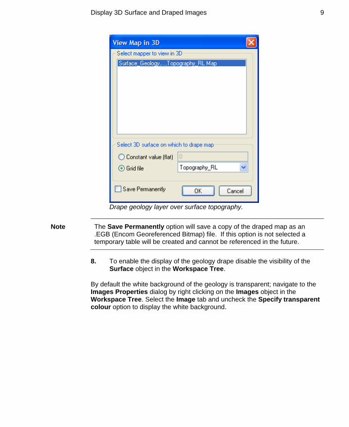
7. With both tables displayed in the mapper, use either the right mouse click View in 3D... or, select Discover3D>View Map in 3D... menu item. Specify the Surface_Geology layer to drape over the Topography_RL surface.
Display 3D Surface and Draped Images 9
Drape geology layer over surface topography.
Note The Save Permanently option will save a copy of the draped map as an .EGB (Encom Georeferenced Bitmap) file. If this option is not selected a temporary table will be created and cannot be referenced in the future.
8. To enable the display of the geology drape disable the visibility of the
Surface object in the Workspace Tree.
By default the white background of the geology is transparent; navigate to the Images Properties dialog by right clicking on the Images object in the Workspace Tree. Select the Image tab and uncheck the Specify transparent colour option to display the white background.

Display 3D Surface and Draped Images 10
Disable colour transparency.
Draped geology layer on surface topography.

Display 3D Surface and Draped Images 11
Step 5 – Drape Air Photo over Surface
The same procedure used for the surface geology can be applied to an airphoto.
9. Within MapInfo Professional, using the layer control, make sure the Airphoto layer visible and ordered above the Topography_RL layer.
With both tables displayed in the mapper, use either the right mouse click View in 3D... or, select Discover3D>View Map in 3D... menu item. Specify the Airphoto layer to drape over the Topography_RL surface.
To enable the display of the airphoto drape disable the visibility of the Surface object and geology drape Images object in the Workspace Tree.
Navigate to the Images Properties dialog by right mouse clicking on the Images object in the Workspace Tree. Select the Transparency tab and move the Transparency slider to 30%. This will alter the display to provide the drape airphoto with a transparency.
Airphoto draped over the surface topography.

Display 3D Surface and Draped Images 12
Step 6 – Offset layers in 3D
From the previous exercises three objects are present in the 3D Display Window, as they were derived from the same surface layer all layers are overlapping. To display all objects it may be necessary to display the layers with an offset.
10. Navigate to the Images Properties dialog for the airphoto drape by right mouse clicking on the Images object in the Workspace Tree. Select the Transform tab, enter an Offset Z value of 50.
11. Navigate to the Surface Properties dialog by right mouse clicking on the Surface object in the Workspace Tree. Select the Surface layer, enter an Offset value of -50.
Specify offset value for surface layer.

Display 3D Surface and Draped Images 13
Surface layers offset in 3D.
Step 7 – Modify Vertical Scale
12. To control the map vertical scaling navigate to the Scale tab of the 3D Map branch properties dialog. The slider associated with the Z Scale controls the vertical exaggeration. Set a Z scale of 2; note the scaling is applied to all datasets within the 3D view.

Display 3D Surface and Draped Images 14
3D Map Properties dialog controlling vertical exaggeration.
Surface layers offset and rescaled in 3D.
Display 3D Surface and Draped Images 15
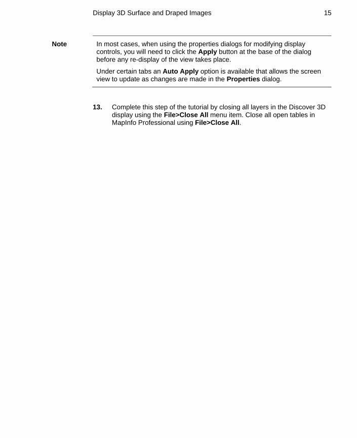
Note In most cases, when using the properties dialogs for modifying display controls, you will need to click the Apply button at the base of the dialog before any re-display of the view takes place.
Under certain tabs an Auto Apply option is available that allows the screen view to update as changes are made in the Properties dialog.
13. Complete this step of the tutorial by closing all layers in the Discover 3D display using the File>Close All menu item. Close all open tables in MapInfo Professional using File>Close All.


Drape Vectors Over Surface 17
3 Drape Vectors Over Surface This tutorial details steps required to drape vector layers over an elevation surface.
A prior level of knowledge navigating in the 3D environment is required. For additional information on MapInfo Professional and Discover, refer to both the MapInfo Professional User Guide and the Discover User Guide.
Step 1 – Open Workspace
1. From the MapInfo Professional menu bar, choose File>Open selecting Files of Type Workspace (*.wor) from the Open dialog. Navigate to the following folder:
Discover 3D\Discover 3D Tutorial\Example Sessions and Workspaces
Open the following workspace file:
Tutorial - Drape Vectors.WOR
Step 2 – Display Draped Airphoto in 3D
2. Navigate to Discover3D>View Map in 3D..., from the View Map in 3D dialog select the mapper to view and the Grid file Topography_RL as the draping surface.

Drape Vectors Over Surface 18
Drape airphoto in 3D.
Airphoto draped over topographic surface.

Drape Vectors Over Surface 19
3. Navigate back to MapInfo Professional and make the vector layers visible using layer control.
Vector layer to make visible include:
Roads
Fences
Streams
Navigate to Discover3D>View Objects in 3D... menu. On the View objects in 3D dialog select the Roads, Fences and Streams tables and Assign a Z value from the grid Topography_RL. This will create separate vector objects in 3D which are draped over the selected surface.
View objects in 3D vector drape.

Drape Vectors Over Surface 20
Vector objects draped in 3D window.
4. If the vector layers are located below the draped airphoto, right click on the Images branch and move to the top of the Workspace Tree or left mouse click and hold on the object and drag to the appropriate location in the Workspace Tree.
Alternatively, navigate to the Images Properties dialog for the airphoto drape by right mouse clicking on the Images object in the Workspace Tree. Select the Transform tab, enter an Offset Z value of -1
Within Discover 3D, you can toggle the display of the vectors from the Workspace Tree by simply unchecking the vectors you wish not to view.
5. If the vector lines are not thick enough access the properties of the vector layers and modify the line style from within the Surface tab.
6. Complete this step of the tutorial by closing all layers in the Discover 3D display using the File>Close All menu item. Close all open tables in MapInfo Professional using File>Close All.
Display Point and Line Data 21
4 Display Point and Line Data This tutorial describes how to display geochemical point data and modify colour based on element values in Discover 3D.
A prior level of knowledge navigating in the 3D environment is required. For additional information on MapInfo Professional and Discover, refer to both the MapInfo Professional User Guide and the Discover User Guide.
Step 1 – Open Workspace
1. From the MapInfo Professional menu bar, choose File>Open selecting Files of Type Workspace (*.wor) from the Open dialog. Navigate to the following folder:
Discover 3D\Discover 3D Tutorial\Example Sessions and Workspaces
Open the following workspace file:
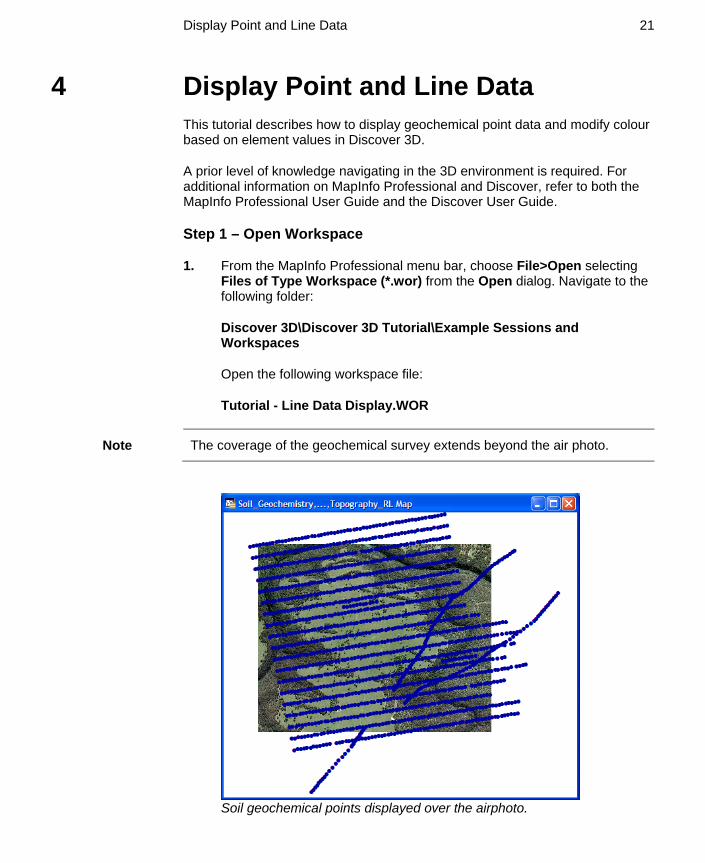
Tutorial - Line Data Display.WOR
Note The coverage of the geochemical survey extends beyond the air photo.
Soil geochemical points displayed over the airphoto.
Display Point and Line Data 22
Step 2 – Display Geochemical Dataset in 3D
2. Display the Airphoto image draped over the Topography_RL surface into the 3D display, navigate to Discover3D>3D Utilities>Overlay Image on Grid.... This will create an EGB file called Airphoto.egb, drop and drag this file into the 3D Display Window from the \Discover 3D Tutorial \Topography folder. Open the 3D Window by navigating to Discover3D>Open 3D Window.
Note Displaying an image draped over a surface with Overlay Image on Grid tool will maintain the full image quality.
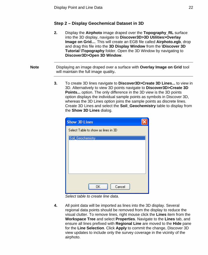
3. To create 3D lines navigate to Discover3D>Create 3D Lines... to view in
3D. Alternatively to view 3D points navigate to Discover3D>Create 3D Points... option. The only difference in the 3D view is the 3D points option displays the individual sample points as symbols in Discover 3D, whereas the 3D Lines option joins the sample points as discrete lines. Create 3D Lines and select the Soil_Geochemistry table to display from the Show 3D Lines dialog.
Select table to create line data.
4. All point data will be imported as lines into the 3D display. Several regional data points should be removed from the display to reduce the visual clutter. To remove lines, right mouse click the Lines item from the Workspace Tree and select Properties. Navigate to the Lines tab, and ensure all lines prefixed with Regional Line are moved to the Hide pane for the Line Selection. Click Apply to commit the change, Discover 3D view updates to include only the survey coverage in the vicinity of the airphoto.

Display Point and Line Data 23
Remove the regional lines using the Lines Properties dialog.
Step 3 – Modifying Line Appearance
Numerous options are present to control the appearance of lines and point data; including style, colour and thickness.
5. Display the Properties dialog of the Lines branch of the Workspace Tree and select the Appearance tab. Click the Line Style button; the dialog presented will allow modification of the line thickness, select weight of 3.5. Click the Apply button to update the display.

Display Point and Line Data 24
Modify Line thickness.
6. Within the survey area, copper is of significant interest. To modulate the line colour based on copper values, navigate to the Colour tab on the Lines Properties dialog, enable the Colour option. From the pull-down list, select Cu. Click the Apply button to display a colour modulated line based on copper values.
7. Further colour enhancement can be performed using the colour
modulation table accessed via the Edit colour scale button. The data lines reflect the changing copper values along the sampled lines.
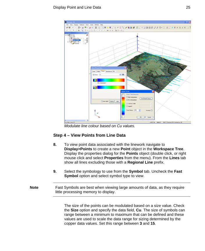
Display Point and Line Data 25
Modulate line colour based on Cu values.
Step 4 – View Points from Line Data
8. To view point data associated with the linework navigate to Display>Points to create a new Point object in the Workspace Tree. Display the properties dialog for the Points object (double click, or right mouse click and select Properties from the menu). From the Lines tab show all lines excluding those with a Regional Line prefix.
9. Select the symbology to use from the Symbol tab. Uncheck the Fast Symbol option and select symbol type to view.
Note Fast Symbols are best when viewing large amounts of data, as they require little processing memory to display.
The size of the points can be modulated based on a size value. Check the Size option and specify the data field, Cu. The size of symbols can range between a minimum to maximum that can be defined and these values are used to scale the data range for sizing determined by the copper data values. Set this range between 3 and 15.

Display Point and Line Data 26
Modulate point size by Cu value.
Step 5 – Colour Modulate Points
10. To highlight copper values colour modulate the points based on copper values. Navigate to the Colour tab and enable the Colour option. From the pull-down list, select Cu. Click the Apply button to display a colour modulated line based on copper vales.
11. Further colour enhancement can be performed using the colour
modulation table accessed via the Edit colour scale button. The points reflect the changing copper values along the sampled lines.

Display Point and Line Data 27
Modulate points by Cu colour.
Step 6 – Offset Point and Line Data
Geochemical trends can be observed in the point and line datasets with modulated colour vales, however, it can be difficult to observe when obscured by the air photo. To overcome, the individual data lines and points can be offset to highlight the value ranges clearly.
12. Navigate to the Fields tab on the Lines Properties dialog. Activate the Offset option and select the Cu data field from the pull-down list. Click the Apply button to offset the lines.
Note Observe how the lines move up and down depending on the copper data value.
13. Repeat this procedure on the Points Properties dialog, activate the
Offset option and select the Cu data field from the pull-down list. For each point, the copper value is added to the Z or elevation and repositioned accordingly.

Display Point and Line Data 28
Modulate point elevation by CU value.
Step 7 – Display Point Information
Within the 3D interface information can be dynamically displayed for individual objects.
14. From the Workspace Tree make the Points object selectable by activating the Select control.
From the Workspace Tree make the Points object browsable by activating the Browse control.
Ensure the Select/Navigate control is activated.
Ensure the Data Window is open and display in 3D by enabling this control from the Main toolbar.
15. Slowly mouse the mouse cursor over point objects in the 3D Display Window, when the mouse hovers over a point, information about that point is displayed in the Data Window.
The Data Window fields can be customised by right mouse clicking in the Data Window and selecting Customise.

Display Point and Line Data 29
16. Complete this step of the tutorial by closing all layers in the Discover 3D display using the File>Close All menu item. Close all open tables in MapInfo Professional using File>Close All.


Display Vector Objects in 3D 31
5 Display Vector Objects in 3D This tutorial shows you how to add various 3D objects into the 3D display. Typically, objects are created in third-party software such as modelling programs, mine planning packages or systems capable of producing 3D output.
A prior level of knowledge navigating in the MapInfo Professional and Discover 3D environment is assumed. For additional information on MapInfo Professional and Discover, refer to both the MapInfo Professional User Guide and the Discover User Guide.
Step 1 – Open Dataset
1. From the MapInfo Professional menu bar, choose File>Open selecting Files of Type Workspace (*.wor) from the Open dialog. Navigate to the following folder:
Discover 3D\Discover 3D Tutorial\Example Sessions and Workspaces
Open the following workspace file:
Tutorial - Display DXF Vectors.WOR
Orebody outline displayed on airphoto.

Display Vector Objects in 3D 32
Step 2 – Display Draped Map in 3D
2. Navigate to Discover 3D>View Map in 3D..., from the View Map in 3D dialog select the mapper to view and the Grid file Topography_RL as the draping surface.
Step 3 – Load DXF in 3D
The most common and versatile 3D data format is the AutoCad DXF 3D format file. This file type is supported by Discover 3D, in some cases and where appropriate the DXF format files can also be displayed in MapInfo Professional and Discover.
3. Two methods are available to import a DXF file directly into Discover 3D.
Select the Display>3D Vector item from the main menu or
Drop-and-Drag the DXF file into Discover 3D from Windows Explorer.
4. Create a new 3D Vector object using Display>3D Vector option. Right mouse click the Vectors item from the Workspace Tree and select Properties. Navigate to the File tab, use the Browse button to specify a 3D DXF file. Navigate to the Orebody Models folder and select the Skarn_Orebody.DXF file.
Click the Apply button after selection to display the orebody.

Display Vector Objects in 3D 33
Skarn orebody displayed in 3D.
Step 4 – Modify DXF Appearance
Discover 3D provides a number of controls to modify the appearance of displayed DXF files. These controls are located on the Vector Properties dialog.
5. Modify the DXF appearance by adjusting the various property controls
• The geometry of the shape can be smoothed by checking the Smooth Surface option on the File tab.
• The native fill colour of the object can be overridden by modifying the Fill Colour on the Surface tab.
• The vertices of the DXF object can be joined by a wireframe to assist in viewing the smoothness of the object. Check the Wireframe option on the Surface tab to enable.
• The transparency of the object can be altered to permit other items such as drillholes of other 3D objects to become visible. On the Transparency tab move the slider to the desired transparency level.

Display Vector Objects in 3D 34
• To prevent self see through of a transparent object check the Prevent seeing an object through itself option on the Transparency tab.
Modified DXF orebody object.
Step 5 – Display Additional DXF Objects
6. Navigate to the following folder:
Discover 3D\Discover 3D Tutorial\Orebody Models
From Windows Explorer Drop-and-Drag the following DXF files into the 3D Display Window:
Shaft.DXF
Fault_1.DXF
Development.DXF

Display Vector Objects in 3D 35
3D DXF files displayed in Discover 3D.
7. Complete this step of the tutorial by closing all layers in the Discover 3D display using the File>Close All menu item. Close all open tables in MapInfo Professional using File>Close All.


Display Drillhole Traces in 3D 37
6 Display Drillhole Traces in 3D This tutorial demonstrates the ability of Discover 3D to visualise and interrogate drillhole data in three dimensions. This has obvious and significant advantages over simply viewing maps and data sections.
A prior level of knowledge navigating in the 3D environment is required. For additional information on how to create, import and display drillhole data, refer to the Drillhole Display section of the Discover User Guide. For additional information on MapInfo Professional and Discover, refer to both the MapInfo Professional User Guide and the Discover User Guide.
Step 1 – Open 3D Dataset
1. From the Discover 3D menu in MapInfo Professional navigate to Discover3D>Open 3D Window. Select the File>Open Session... menu item and navigate to the following folder:
Discover 3D\Discover 3D Tutorial\Example Sessions and Workspaces
Open the following session file:
Tutorial - Drillhole Surface Drape.EGS
Step 2 – Import Drillhole Project
2. Navigate to the Drillhole menu item in Discover to open a supplementary Drillholes menu. Select Drillholes>Project Manager>Import/Export. Navigate to the following folder:
Discover 3D\Discover 3D Tutorial\Drilling Data\Drillhole Project
Import the following drillhole project file:
Example Drilling.setup.xml
When prompted by Discover import the project and accept the default name Example Drilling. Click OK.

Display Drillhole Traces in 3D 38
Import Discover Drillhole Project.
From Drillholes menu navigate to Drillholes>Project Manager... and select the Example Drilling project. Click Open.
Open Discover Drillhole Project.
A mapper window containing the Drillhole_Collar table and TOPOGRAPHY_RL grid will open with the project. The other required project tables Drillhole_LITH, Drillhole_SURVEYS, Drillhole_ASSAYS will open in the background.

Display Drillhole Traces in 3D 39
Step 3 – Display Drillhole Traces in 3D
3. Navigate to the Discover3D>View Drillholes... option. Select all the drillholes by clicking the Select All button on the 3D Drillhole Wizard dialog.
Import drillholes into Discover 3D.
Note For very large datasets or for lower-end computers, it is advisable to import only a subset of the drillhole dataset into the 3D window. To do this, tick the Load Subset based on selected option at the bottom of the dialog, ensure that only the drillholes to be imported are listed under the Selected column.
Initially, drillhole traces are displayed as grey 3D tubes. The collar positions of the drillholes coincide with the topographic surface that has the Airphoto draped over it.

Display Drillhole Traces in 3D 40
Drillhole traces displayed in Discover 3D.
Step 4 - Selecting Drillholes in Discover 3D
4. Right mouse click on the Drillholes object on the Workspace Tree
and select the Properties option. Navigate to the Holes tab, click the Drillhole Selection button.
From the Drillhole Selection dialog use the Selection Tools to select a subset of the drillholes to display in 3D. Click Apply, only the selected holes will be displayed.
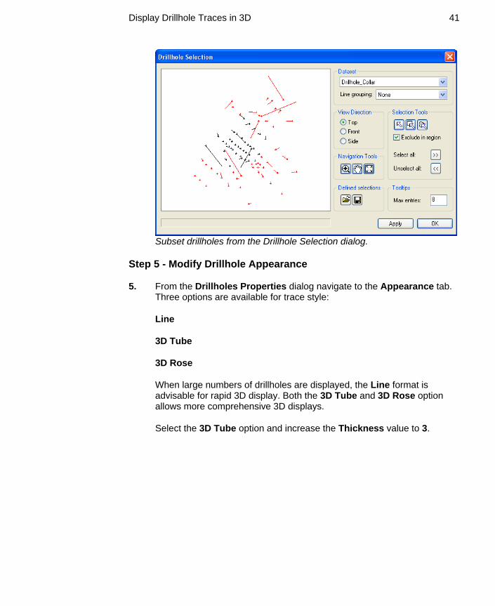
Display Drillhole Traces in 3D 41
Subset drillholes from the Drillhole Selection dialog.
Step 5 - Modify Drillhole Appearance
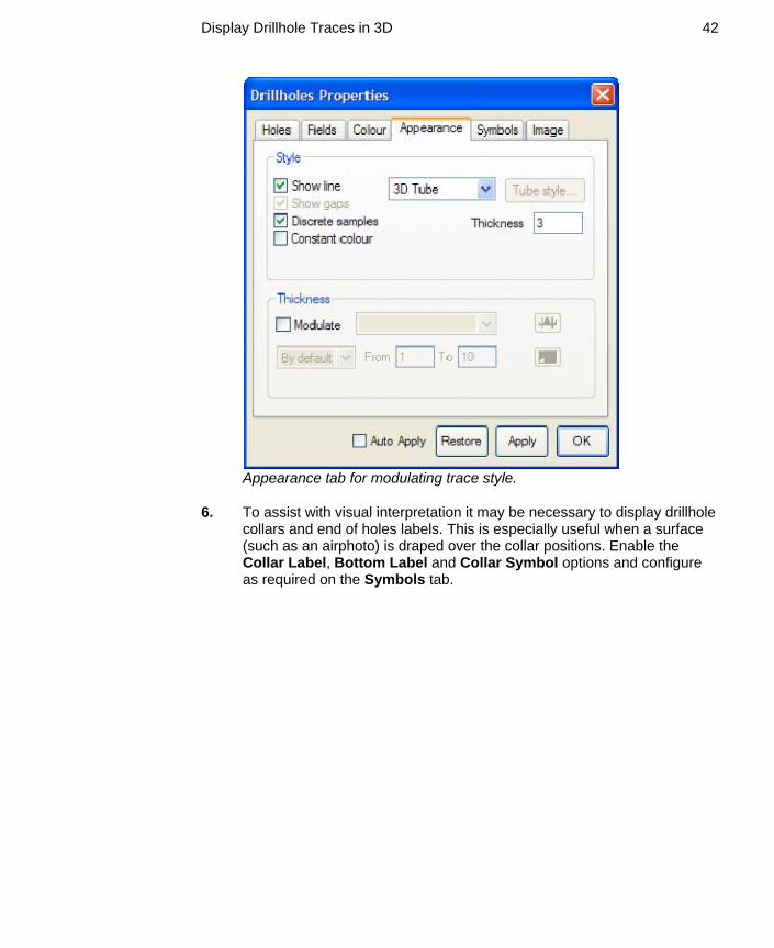
5. From the Drillholes Properties dialog navigate to the Appearance tab. Three options are available for trace style:
Line
3D Tube
3D Rose
When large numbers of drillholes are displayed, the Line format is advisable for rapid 3D display. Both the 3D Tube and 3D Rose option allows more comprehensive 3D displays.
Select the 3D Tube option and increase the Thickness value to 3.
Display Drillhole Traces in 3D 42
Appearance tab for modulating trace style.
6. To assist with visual interpretation it may be necessary to display drillhole collars and end of holes labels. This is especially useful when a surface (such as an airphoto) is draped over the collar positions. Enable the Collar Label, Bottom Label and Collar Symbol options and configure as required on the Symbols tab.

Display Drillhole Traces in 3D 43
Modify Drillhole labels and symbols.
Step 6 - Modulate Drillhole Thickness
7. Navigate to the Appearance tab and select 3D Rose drillhole style. The Petals button controls the display thickness of the drill trace based on selected downhole attributes such as assay values. Select this option to display the Petal Channels dialog. The colour, size and data fields displayed are controlled from this dialog.
The Petal Channels dialog controls the tube thickness of drillholes as either discs or enlarged tubes. Check the Show box to activate a field to display, specify a Field to control the drillhole diameter. Select the Drillhole_ASSAYS_AU_AVG from the Field pull-down list. Ensure both the Enhance and Global options are checked to modulate the thickness.
Click the Apply button, note how the displayed drillhole diameters alter. Multiple data channels can be selected to control thickness with multiple drillhole diameters relative to the data channels selected. Experiment with modulation of the drillhole traces using multiple assay fields.

Display Drillhole Traces in 3D 44
Modulate trace thickness by assay value.

Display Drillhole Traces in 3D 45
Modulated drillhole thickness by Drillhole_ASSAYS_CU and Drillhole_ASSAY_AU_AVG.
Note Performance degradation may be experienced when visualising drill traces as 3D Rose Petals. For faster navigation speed use either 3D Tube or Line trace styles.
Step 7 - Modulate Drillhole Colour
8. Ensure the drill trace is thickness modulated only by the Drillhole_ASSAYS_AU_AVG field. Navigate to the Colour tab and check the Colour box. This feature allows the colour of the drillholes to change depending on values contained within a data field. For example, drillhole assays or lithology can be used to alter not only the colour, but also the patterns of display of the drillholes.
9. Select the Drillhole_ASSAYS_AU_AVG from the pull-down list. To select a specific colour scheme or legend to colour or attribute the drillhole traces, click the Apply button.

Display Drillhole Traces in 3D 46
The colour applied to the drill traces is relatively uniform; this is due to the presence of null assay values expressed as -1 value. To display a colour scheme which reflects the data better select the Edit Colour Mapping button. Check the Apply bandpass cutoff box and type in a lower and upper value of 5% and 95% respectively. Click OK to commit the change.
Colour Mapping with cut-off applied to upper and lower data values.

Display Drillhole Traces in 3D 47
Modulated drillhole thicknesses by thickness and colour.
Extensive control is provided over the selection and appearance of the available look-up tables and legends that provide colours or patterns to the drillholes, custom LUT tables and legends can be constructed. A range of look-up tables are supplied with Discover 3D as well as a powerful Colour Lookup Editor (refer to the Discover 3D User Guide).
Look-up tables control the colours used in modulating the drillhole data, in addition, patterns can be used instead. Patterns use available Legends also supplied with the software, or you can use the Legend Editor to create and edit these (refer to the Legend Editor in the Discover 3D User Guide).
10. Complete this step of the tutorial by closing all layers in the Discover 3D display using the File>Close All menu item. Close all open tables in MapInfo Professional using File>Close All.

Display Drillhole Traces in 3D 48
Example drill trace modulation.
Drill trace modulated by lithology.

Display Drillhole Sections in 3D 49
7 Display Drillhole Sections in 3D This tutorial illustrates how interpreted drillhole sections can be displayed in a 3D view with the associated drillhole information. From drillhole data, logs, rock type or assay data interpretations can be created within Discover 3D. When these interpretations are displayed in three dimensions their relationships can become significantly more meaningful.
A prior level of knowledge navigating in the 3D environment is required. For additional information on how to create, import and display drillhole data, refer to the Drillhole Display section of the Discover User Guide. For additional information on MapInfo Professional and Discover, refer to both the MapInfo Professional User Guide and the Discover User Guide.
Step 1 – Open 3D Dataset
1. From the Discover 3D menu in MapInfo Professional navigate to Discover3D>Open 3D Window. Select the File>Open Session... menu item and navigate to the following folder:
Discover 3D\Discover 3D Tutorial\Example Sessions and Workspaces
Open the following session file:
Tutorial - Drillhole Section Display.EGS
Step 2 – Open Discover Drillhole Project
2. From the MapInfo Professional menu bar, navigate to Discover>Drillholes>Project Manager.... From the Project Manager select the project Example Drilling to open. If this project is not visible you will need to import as described in the Display Drillhole Traces in 3D tutorial.
3. Navigate to Drillholes>Section Manager... and open the three previously created sections; Section_1, Section_2 and Section_3. From the Section Manager dialog, select all three available sections and then click the Open button. The digitized polygon represents a lithology layer consisting of a Lava unit.

Display Drillhole Sections in 3D 50
Display drillhole sections in MapInfo.
Step 3 – Display Sections in 3D
4. Navigate to Discover3D>View Sections... to export the open section into 3D. Highlight all three sections on the Export located bitmap dialog and click OK. Ensure only the sections are highlighted since other windows such as the collar map are inappropriate to display as sections.
Export Drillhole sections to Discover 3D.

Display Drillhole Sections in 3D 51
Drillholes sections display in Discover 3D.
5. Complete this step of the tutorial by closing all layers in the Discover 3D display using the File>Close All menu item. Close all open tables in MapInfo Professional using File>Close All.


Create 3D Object from Section Boundary 53
8 Create 3D Object from Section Boundary This tutorial illustrates how to create a 3D solid object from a series of digitized drillhole section boundary layers.
A prior level of knowledge navigating in the MapInfo Professional and Discover 3D environment is assumed. For additional information on MapInfo Professional and Discover, refer to both the MapInfo Professional User Guide and the Discover User Guide.
What are Feature Objects and Feature Database?
The feature database provides a powerful utility for the creation and storage of 3D Feature Objects. Feature Objects are points, lines or polygonal regions that represent entities such as geological/ore boundaries, structural/fault intersections or other general features of interest in the 3D environment. These objects can be created in Discover3D, exported from MapInfo Professional or imported from third party software.
Feature Objects are stored in a Feature Database. A Feature Database contains a Feature Dataset, e.g. supergene ore boundaries or interpreted fault lines. Attribute data can be added to these objects as seamless in MapInfo Professional. Feature objects can also be queried for volume and 3D solid bodies created.
Step 1 – Open 3D Dataset
1. From the Discover 3D menu in MapInfo Professional navigate to Discover3D>Open 3D Window. Select the File>Open Session... menu item and navigate to the following folder:
Discover 3D\Discover 3D Tutorial\Example Sessions and Workspaces
Open the following session file:
Tutorial - Drillhole Create Solid.EGS
Step 2 – Open Discover Drillhole Project
2. From the MapInfo Professional menu bar, navigate to Discover>Drillholes>Project Manager.... From the Project Manager select the project Example Drilling to open. If this project is not visible you will need to import as described in the Display Drillhole Traces in 3D tutorial.

Create 3D Object from Section Boundary 54
3. Navigate to Drillholes>Section Manager... and open the three previously created sections; Section_1, Section_2 and Section_3. From the Section Manager dialog, select all three available sections and then click the Open button. The digitized polygon represents a lithology layer consisting of a Lava unit. We are going to create a solid object from these digitized boundaries to display in 3D.
Step 3 – Display Section Boundaries in 3D
4. Navigate to Discover3D>View Section Layers... to export the open section boundaries into 3D. Highlight all three sections on the Export Boundary to 3D Feature dialog. Under Output click the Save button and rename the Feature Database to Section Layers, click OK. This will create a Feature Database with all the section boundaries.
5. The Features Properties dialogue will appear. It is possible to colour code features determined by feature type. This function relies on the user populating the Feature Code column when the boundaries are digitised in MapInfo Professional. Navigate to MapInfo Professional and open the Browser of the section table Section_1B. Feature Code information such as boundary details can be entered. If desired enter information for all three sections and re-import to display colour by this field.
Digitized boundaries imported into 3D.

Create 3D Object from Section Boundary 55
Step 4 – Create Solid Object
6. Navigate to Utilities>3D Solid Generator.... Select Section Boundaries from the Sections drop down menu. Choose a surface colour from the Surface Colour drop down menu and select Smooth from the End Capping Style drop down menu. Click Apply, in the 3D preview window the generated 3D object can be viewed. A report containing the calculated body volume is also created. If the interpolation between the Feature Objects is not satisfactory then tie lines can be added to aid the interpolation process. Click Close.
The 3D Feature Solid is displayed as a 3D DXF file, and represents the Lava lithological unit.
7. Complete this step of the tutorial by closing all layers in the Discover 3D display using the File>Close All menu item. Close all open tables in MapInfo Professional using File>Close All.
3D solid created with the 3D Solid Generator.


Display Georeferenced Image Slice 57
9 Display Downhole Logs in 3D The objective of this tutorial is to display downhole log plot in 3D.
A prior level of knowledge navigating in the 3D environment is required. For additional information on how to create, import and display drillhole data, refer to the Drillhole Display section of the Discover User Guide. For additional information on MapInfo Professional and Discover, refer to both the MapInfo Professional User Guide and the Discover User Guide.
Step 1 – Open 3D Dataset
1. From the Discover 3D menu in MapInfo Professional navigate to Discover3D>Open 3D Window. Select the File>Open Session... menu item and navigate to the following folder:
Discover 3D\Discover 3D Tutorial\Example Sessions and Workspaces
Open the following session file:
Tutorial - Drillhole Log Display.EGS
Step 2 – Open Discover Drillhole Project and logs
2. From the MapInfo Professional menu bar, navigate to Discover>Drillholes>Project Manager.... From the Project Manager select the project Example Drilling to open. If this project is not visible you will need to import as described in the Display Drillhole Sections in 3D tutorial.
3. From the MapInfo Professional menu bar, choose File>Open selecting Files of Type Workspace (*.wor) from the Open dialog. Navigate to the following folder:
Discover 3D\Discover 3D Tutorial\Example Sessions and Workspaces
Open the following workspace file:
Tutorial - Drillhole Logs.WOR

Display Georeferenced Image Slice 58
Step 3 – Display Logs in 3D
4. Select the Discover3D>View Logs... menu item to display logs in 3D. Check the Best Fit option, the will locate the lending edge of the log adjacent to the drill trace, otherwise the log may appear separated from the drill trace. Click OK to display logs in 3D.
Export drillhole logs to Discover 3D.
To reduce the display clutter navigate to the Holes tab on the Drillholes Properties dialog and only select the following holes to display; AN3069, AN3141, AN3142 and AN3159

Display Georeferenced Image Slice 59
Display of drillholes and associated logs.
Step 4 – Modifying Appearance of Logs
5. From the Drillholes Properties dialog navigate to the Image tab. Experiment with the various options for the log display, increase the image quality, transparency etc.
Adjust the Azimuth and Scale (horizontal) using the provided slider bars. Note that the purpose of the azimuth and scale controls is to allow for rotation of the 3D display. To optimally view the logs, rotate them towards a uniform azimuth; enable the Uniform Azimuth option and then use the Azimuth slider to control their orientation.
6. Complete this step of the tutorial by closing all layers in the Discover 3D display using the File>Close All menu item. Close all open tables in MapInfo Professional using File>Close All.

Display Georeferenced Image Slice 60
10 Display Georeferenced Image Slice This tutorial describes how to export a geo-located image from 3D into MapInfo Professional.
A prior level of knowledge navigating in the MapInfo Professional and Discover 3D environment is assumed. For additional information on MapInfo Professional and Discover, refer to both the MapInfo Professional User Guide and the Discover User Guide.
This is a powerful way to capture slices through a dataset (e.g. Voxel models, .DXF solid models) as georeferenced images.
Georeferenced images can used in the following ways:
• Display in other software applications (e.g. PowerPoint or Word).
• Efficient display in Discover 3D of more complex and memory-intensive datasets (e.g. displaying a Voxel model as a series of image slices).
• Export to associated Discover drillhole cross-sections for detailed data comparison and interpretation.
Step 1 – Open 3D Dataset
1. From the Discover 3D menu in MapInfo Professional navigate to Discover3D>Open 3D Window. Select the File>Open Session menu item and navigate to the following folder:
Discover 3D\Discover 3D Tutorial\Example Sessions and Workspaces
Open the following session file:
Tutorial - Display Section in 2D.EGS
Step 2 – Open Discover Drillhole Project
2. From the MapInfo Professional menu bar, navigate to Discover>Drillholes>Project Manager.... From the Project Manager select the project Example Drilling to open. If this project is not visible you will need to import as described in the Display Drillhole Traces in 3D tutorial.
3. Navigate to Drillholes>Section Manager... and open the three previously created sections; Section_1, Section_2 and Section_3. From

Display Georeferenced Image Slice 61
the Section Manager dialog, select all three available sections and then click the Open button.
Step 3 – Display Sections in 3D
4. Navigate to Discover3D>View Sections... to export the open section into 3D. Highlight all three sections on the Export located bitmap dialog and click OK. Ensure only the sections are highlighted since other windows such as the collar map are inappropriate to display as sections.
5. Navigate to the following folder
Discover 3D\Discover 3D Tutorial\Orebody Models
Open the following DXF files into 3D:
Shaft.DXF
Skarn_Orebody.DXF
Development.DXF
Step 4 – Export Georeferenced Image from 3D
6. From Discover 3D navigate to Tools>Georeferenced Image Export.... From the Locate image using dropdown select Discover Section. From Discover Section dropdown select Section_1. Change the Clip option to Slice with a Width (total) of 100. Set the Resolution (Pixels): to 2048. Click the Preview button to display the selected settings. Click Apply to create image.

Display Georeferenced Image Slice 62
Georeferenced Image Exporter dialog.
Step 5 – View Geolocated Image in Discover & Discover3D
7. Close the Georeferenced Image Exporter dialog. Navigate to MapInfo Professional, choose cross section window containing the Section_1 section as the front mapper window, the georeferenced image is automatically added to the appropriate section window.
8. Complete this step of the tutorial by closing all layers in the Discover 3D display using the File>Close All menu item. Close all open tables in MapInfo Professional using File>Close All.

Display Georeferenced Image Slice 63
Discover cross section with georeferenced Image of a Skarn orebody and aerial image exported from the Discover 3D window.

Display Voxel Block Model in 3D 64
11 Display Voxel Block Model in 3D This tutorial illustrates the capability of Discover 3D to display complex 3D objects that are constructed from Voxels (‘volume elements’). This type of object is complex and is available from only a few specialist simulation and modelling packages (such as Vulcan, Gemcom, Surpac and DataMine).
A prior level of knowledge navigating in the MapInfo Professional and Discover 3D environment is assumed. For additional information on MapInfo Professional and Discover, refer to both the MapInfo Professional User Guide and the Discover User Guide.
What are voxel models?
The term ‘Voxel’ refers to a volume element and is the three dimensional equivalent of the two dimensional ‘pixel’. As used in mine planning and geophysical modelling, Voxel models represent volumes of the earth which are subdivided in a regular way into sub-volumes, or cells. Each cell, created from six sides contains an earth volume of uniform property attribute. Such properties as rock type, magnetic susceptibility, gravity density, conductivity or IP property (e.g. chargeability or phase) can be used.
Individual cell volumes for display in Discover 3D are prismatic in shape but Voxel models need not be. For example, complex mesh designs are possible whereby individual cell dimensions vary for each of their 12 side lengths.
Example Voxel model.
Step 1 – Open 3D Dataset
1. From the Discover 3D menu in MapInfo Professional navigate to Discover3D>Open 3D Window. Select the File>Open Session... menu item and navigate to the following folder:

Display Voxel Block Model in 3D 65
Discover 3D\Discover 3D Tutorial\Example Sessions and Workspaces
Open the following session file:
Tutorial - Display Voxel.EGS
Step 2 – Load Voxel Model in 3D
The Voxel Model to be used in this tutorial uses the UBC standard format. The model is defined by two files. The first is a descriptive header file (called a MSH file) that specifies the number of rows, columns and branches plus the origin and Voxel sizes.
A second file (called a data file) contains the property values associated with each of the Voxel cells making up the model.
2. Within Discover 3D either click the Display Voxel Model button or select the Display>Voxel Model... menu item. A new Voxel Model branch is added to the Workspace Tree of Discover 3D. Display the Voxel Model properties dialog by right mouse clicking and selecting Properties. Navigate to the File tab and click the Load Model Wizard button. Select the UBC 3D (University of British Columbia) voxel format to import.
Load UBC Voxel Model in Discover 3D.
3. The two required files are contained in folder Discover 3D\Discover 3D Tutorial\Geophysics. The model is the result of a geophysical inversion program that builds a 3D Voxel model and computes the magnetic susceptibility property for each cell. The data files required are:

Display Voxel Block Model in 3D 66
Mesh.msh (Mesh file)
Maginv3d.sus (Data file)
Select Finish and Apply to display the Voxel model.
UBC Voxel model display in Discover 3D.
Step 3 – Modify Voxel Model Appearance
Many operations can be performed on the Voxel model to view the internal structure and properties of the volume.
Available operations include:
• Thresholding
• Isosurfacing
• Offsetting
• Colour filling
• Clipping
Display Voxel Block Model in 3D 67
• Slice display
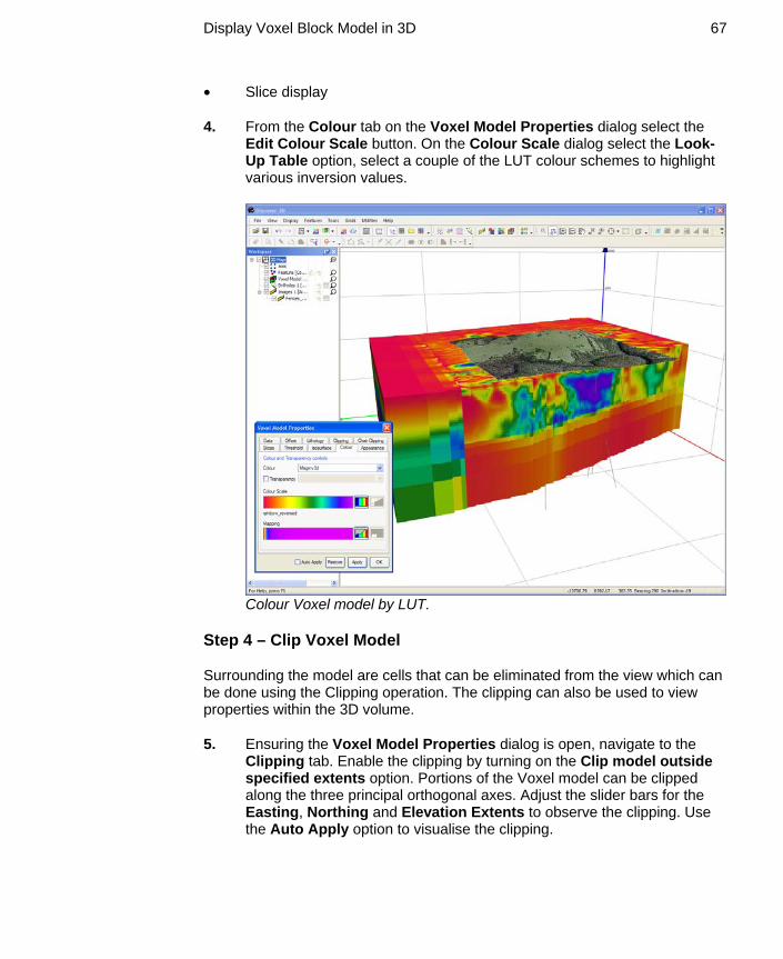
4. From the Colour tab on the Voxel Model Properties dialog select the Edit Colour Scale button. On the Colour Scale dialog select the Look-Up Table option, select a couple of the LUT colour schemes to highlight various inversion values.
Colour Voxel model by LUT.
Step 4 – Clip Voxel Model
Surrounding the model are cells that can be eliminated from the view which can be done using the Clipping operation. The clipping can also be used to view properties within the 3D volume.
5. Ensuring the Voxel Model Properties dialog is open, navigate to the Clipping tab. Enable the clipping by turning on the Clip model outside specified extents option. Portions of the Voxel model can be clipped along the three principal orthogonal axes. Adjust the slider bars for the Easting, Northing and Elevation Extents to observe the clipping. Use the Auto Apply option to visualise the clipping.

Display Voxel Block Model in 3D 68
Clip Voxel Model along 3 principle axes.
Another method of clipping the model is called Chair Clipping. This operation can clip in all three principal axis directions at once to display internal structure.
6. Select the Chair Clipping tab, enable the Chair clipping by turning on the Clip model with specified extents Front and Back standard cuts => option. Click one of the Top Left (TL), Top Right (TR) etc buttons to initiate the chair clipping and then use the sliders to cut through different directions of the model.

Display Voxel Block Model in 3D 69
Chair Clipping the Voxel Model to reveal internal structure.
Step 5 – Threshold Voxel Model
A useful method of visualising a volume is to display only those cells that have a data property above or within a specific data range. This process is referred to as thresholding.
7. Disable the Clipping and Chair Clipping options to revert back to a display with all cells that are not clipped. Navigate to the Threshold tab and enable the Threshold option by Maginv3d.sus property. Ensure the Auto Apply option is enabled.
8. Set the Transparency slider bar to approximately 30%; this controls the transparency of the displayed thresholded data. Slide the Accept Voxel Range sliders at the base of the dialog, cells within the upper and lower range will only be visible. Set the upper and lower ranges to be about 0.03 to 0.05 for optimal anomaly viewing.
Display Voxel Block Model in 3D 70
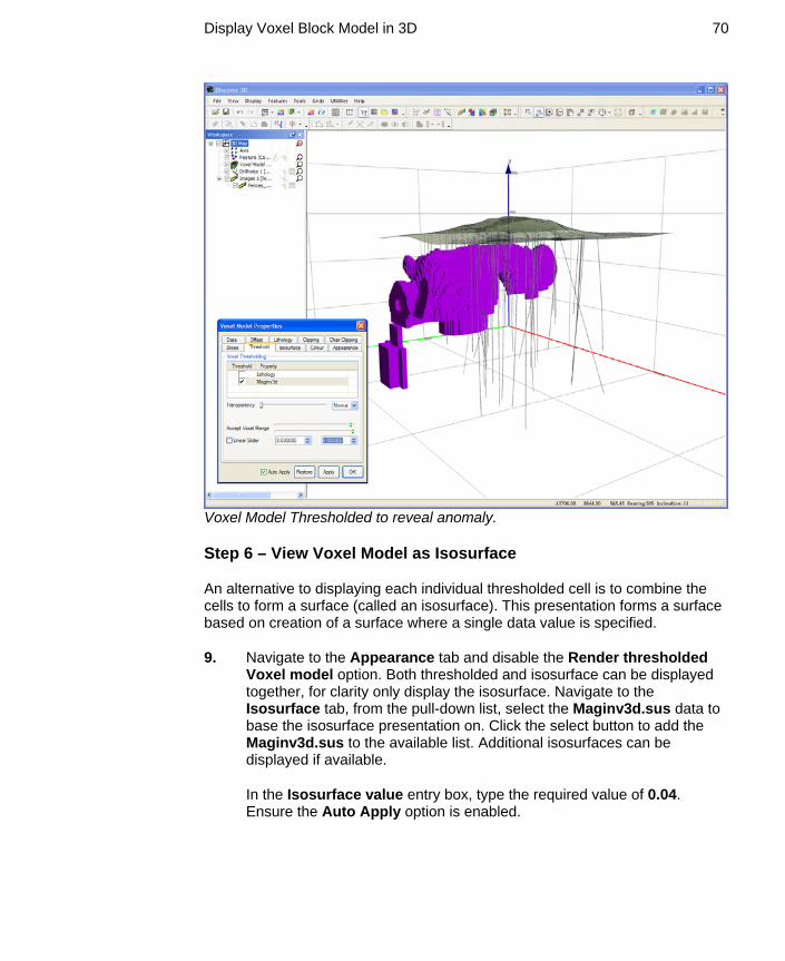
Voxel Model Thresholded to reveal anomaly.
Step 6 – View Voxel Model as Isosurface
An alternative to displaying each individual thresholded cell is to combine the cells to form a surface (called an isosurface). This presentation forms a surface based on creation of a surface where a single data value is specified.
9. Navigate to the Appearance tab and disable the Render thresholded Voxel model option. Both thresholded and isosurface can be displayed together, for clarity only display the isosurface. Navigate to the Isosurface tab, from the pull-down list, select the Maginv3d.sus data to base the isosurface presentation on. Click the select button to add the Maginv3d.sus to the available list. Additional isosurfaces can be displayed if available.
In the Isosurface value entry box, type the required value of 0.04. Ensure the Auto Apply option is enabled.

Display Voxel Block Model in 3D 71
Display Voxel Model Isosurface
Step 7 – View the Voxel Model with Other Objects
10. Navigate to the following folder
Discover 3D\Discover 3D Tutorial\Orebody Models
Open the following DXF files into 3D:
Shaft.DXF
Skarn_Orebody.DXF
Development.DXF
Within the 3D window toggle the visibility and colour of the various objects present in the Workspace Tree to visualise the data interrelationships.

Display Voxel Block Model in 3D 72
Isosurface Voxel Model
11. Complete this step of the tutorial by closing all layers in the Discover 3D display using the File>Close All menu item. Close all open tables in MapInfo Professional using File>Close All.