Discounts for Lack of Marketability...Abstract Discount for Lack of Marketability (DLOM) is one of...

IN THE FIELD OF TECHNOLOGYDEGREE PROJECT VEHICLE ENGINEERINGAND THE MAIN FIELD OF STUDYINDUSTRIAL MANAGEMENT,SECOND CYCLE, 30 CREDITS

, STOCKHOLM SWEDEN 2017

Discounts for Lack of MarketabilityAn investigation of industry and region influences on the discount

JOSEPHINE MAGNUSSON

MAX TALBAK

KTH ROYAL INSTITUTE OF TECHNOLOGYSCHOOL OF INDUSTRIAL ENGINEERING AND MANAGEMENT

Avdrag för Bristande Likviditet: En undersökning av skillnader i avdraget

mellan industrier och regioner

av

Josephine Magnusson Max Talbak

Examensarbete INDEK 2017:100 KTH Industriell teknik och management

Industriell ekonomi och organisation SE-100 44 STOCKHOLM

Discounts for Lack of Marketability: An investigation of industry and region

influences on the discount

Josephine Magnusson Max Talbak

Master of Science Thesis INDEK 2017:100 KTH Industrial Engineering and Management

Industrial Management SE-100 44 STOCKHOLM

Examensarbete INDEK 2017:100

Avdrag för Bristande Likviditet: En undersökning av skillnader i avdraget

mellan industrier och regioner

Josephine Magnusson

Max Talbak

Godkänt

2017-06-02

Examinator

Terrence Brown

Handledare

Tomas Sörensson Uppdragsgivare

PwC Sverige Kontaktperson

Jon Walberg

Sammanfattning Avdrag för bristande likviditet (DLOM) är en av de mest substantiella justeringarna som

appliceras vid värdering av privatägda bolag, på grund av att marknaden värderar privatägda

bolag lägre än publika motsvarigheter. Denna studie syftar till att analysera och uppskatta det

använda avdraget för bristande likviditet inom olika typer av bolag baserat på deras industri- och

nationella tillhörighet. En regressionsanalys av jämförelser mellan IPO-priser och tidigare

genomföra transaktioner inom respektive bolag visade att Europeiska företag har ett lägre

DLOM än Amerikanska företag, och att industritillhörigheten har en betydelse för storleken på

avdraget. Det Europeiska urvalet hade en median av DLOM på 39% jämfört med Amerikanska

marknaden som hade en median motsvarande 47%, och baserat på företagens industritillhörighet

varierade rabatten med en median på 31% och 56%. För enskilda bolag kan skillnader i DLOM

förklaras av olika värderingsrelaterade faktorer såsom tillväxt, lönsamhet och risk. Resultaten i

studien visar vidare att skillnaderna i DLOM mellan industrier förklaras av transaktionsfrekvens

(inklusive IPO:s), där t.ex. tjänstesektorn har en median av DLOM på 50% medan gruvsektorn

har ett DLOM på 37%. Möjliga synergier vid M&A:s och riskkapitaltillflöde inom industrin ges

också som förklaringar till skillnaderna i DLOM mellan industrierna. Skillnaderna mellan USA

och Europa diskuteras utifrån den amerikanska marknadens högre likviditet, lägre kostnader för

transaktioner och dollarns styrka. Den europeiska marknaden är mer volatil och mindre homogen

och karaktäriseras i högre grad av bankutlåning, medan den amerikanska karaktäriseras av

obligationslösningar och en mer mogen riskkapitalmarknad med större genomlysning och

transparens.

Nyckelord: Likviditet, Företagsvärdering, IPO, Avdrag, DLOM

Abstract Discount for Lack of Marketability (DLOM) is one of the most substantial adjustments applied

on a valuation of privately held companies, and it can be seen that the market values privately

held companies lower than publicly traded equivalents. This study intends to analyze and

estimating the resulting discount for lack marketability for different types of companies based on

their industry-/ national affiliation. A regression analysis of comparison between IPO prices and

previous transactions showed that European companies are subject to a lower DLOM than U.S.

equivalents, and that the industry has an influence on the amount of discount applied. The

European sample has a median DLOM of 39% compared to the US market with a median

equivalent to 47%, and the industries varied with a median of 31% and 56%. For individual

companies, the differences in DLOM can be explained by different valuation-related factors such

as growth, profitability and risks. Further, the result show that differences between industries are

explained by the transaction frequency (including IPOs), where e.g. the service sector had a

higher DLOM, 50%, while the mining sector has a lower DLOM of 37% respectively. Possible

company specific synergies of M&A’s and venture capital are also given as an explanation for

the differences in DLOM between industries. The differences between the U.S. and Europe are

discussed based on the higher liquidity in the public traded sector, lower transaction costs and

currency effects. The European market is more volatile, less homogeneous and more

characterized by bank lending, while the U.S. market is characterized by corporate bond issuing

and a more mature venture capital market with more transparency.

Key-words: Marketability, Valuation, IPO, Discounts, DLOM

Master of Science Thesis INDEK 2017:100

Discounts for Lack of Marketability: An investigation of industry and region

influences on the discount

Josephine Magnusson

Max Talbak

Approved

2017-06-02 Examiner

Terrence Brown Supervisor

Tomas Sörensson Commissioner

PwC Sverige Contact person

Jon Walberg

List of Abbreviations

ANOVA Analysis of Variance ASA American Society of Appraisers AECA Spanish Accounting and Business Administration

Association BV Book Value DCF Discounted Cash Flow model DLOM Discount for Lack of Marketability EBITDA Earnings Before Interest, Taxes, Depreciation and

Amortization EV Enterprise Value FCF Free Cash Flow FCFF Free Cash Flow to Firm FMV Fair Market Value FV Fair Value IPO Initial Public Offering IV Investment Value SEC Securities Exchange Commission IRS Internal Revenue Service LEAP Long-term Equity Anticipation Program LTM Last Twelve Months NAICS North American Industrial Classification Standard NAV Net Asset Value P Share Price QMDM Quantitative Marketability Discount Model SIC Standard Industrial Classification SEC Securities Exchange Commission TEGoVA The European Group of Valuation Associations WACC Weighted Average Cost of Capital

Table of Contents 1 Introduction ......................................................................................... 2

1.1 Background ...................................................................................................................... 2 1.2 Problematization .............................................................................................................. 3 1.3 Purpose ............................................................................................................................. 4 1.4 Research questions ........................................................................................................... 4 1.5 Delimitations .................................................................................................................... 5 1.6 Expected contribution ...................................................................................................... 5 1.7 Disposition ....................................................................................................................... 6

2 Literature and Theory ........................................................................... 8 2.1 Efficient Market Hypothesis ............................................................................................ 8 2.2 Value ................................................................................................................................. 9

2.2.1 Fair Market Value ....................................................................................................... 10 2.2.2 Other definitions on value .......................................................................................... 10 2.2.3 Appraising value ......................................................................................................... 10

2.3 Relation between Efficient Market Hypothesis and Marketability Discounts .............. 11 2.4 Marketability and Liquidity ........................................................................................... 12

2.4.1 Factors affecting marketability .................................................................................. 13 2.5 Discounts and premiums ............................................................................................... 14

2.5.1 Discounts of lack of Marketability for controlling and non-controlling interests ..... 15 2.6 Initial Public Offerings ................................................................................................... 16

2.6.1 The effects of IPOs on business value ......................................................................... 17 2.7 Previously accredited studies for Discounts for Lack of Marketability ........................ 18

2.7.1 Restricted Stock studies ............................................................................................. 18 2.7.2 Pre-IPO studies .......................................................................................................... 19 2.7.3 Theoretical models ..................................................................................................... 21 2.7.4 Summary of models ................................................................................................... 23

2.8 DLOM in the courts ........................................................................................................ 24 2.8.1 European juridical cases ............................................................................................ 27

2.9 Summary of theoretical assumptions ............................................................................ 27 2.9.1 Suggested model for determining DLOM .................................................................. 28

3 Method ............................................................................................... 29 3.1 Methodological approach and research design ............................................................. 29

3.1.1 Choice of quantitative method ................................................................................... 29 3.2 Literature collection ....................................................................................................... 30 3.3 Regression analysis ........................................................................................................ 30

3.3.1 Linear Regression model ........................................................................................... 31 3.3.2 R-square ..................................................................................................................... 33 3.3.3 Multicollinearity ......................................................................................................... 34 3.3.4 Homoscedasticity ....................................................................................................... 36 3.3.5 P-value ........................................................................................................................ 38 3.3.6 F-test for joint null-hypothesis .................................................................................. 38 3.3.7 Analysis of Variance ................................................................................................... 39 3.3.8 Pros and cons with using a linear regression model ................................................. 40

3.4 Method for Research question 1 .................................................................................... 41 3.4.1 Choice of variables ..................................................................................................... 41 3.4.2 Data processing and analysis ..................................................................................... 41 3.4.3 Method for regression analysis .................................................................................. 42 3.4.4 Interpretation of results ............................................................................................. 43

3.5 Method for Research Question 2 ................................................................................... 43 3.5.1 Choice of variables ..................................................................................................... 43 3.5.2 Data processing and analysis ..................................................................................... 44 3.5.3 Method for regression analysis .................................................................................. 45 3.5.4 Interpretation of results ............................................................................................. 45

3.6 Summary of method ....................................................................................................... 45

4 Data collection .................................................................................... 47 4.1 Gathering of data ............................................................................................................ 47 4.2 Raw data ......................................................................................................................... 48 4.3 Preparation for Research Question 1 ............................................................................. 50

4.3.1 Data analysis ............................................................................................................... 51 4.3.2 European data analysis .............................................................................................. 52 4.3.3 Removing outliers ...................................................................................................... 53

4.4 Preparation for Research Question 2 ............................................................................. 53 4.4.1 Data analysis .............................................................................................................. 53

5 Results and Analysis ............................................................................ 55 5.1 Regression analysis on regional markets ....................................................................... 55

5.1.1 Tests for multicollinearity and heteroscedasticity .................................................... 55 5.1.2 Linear regression results ............................................................................................ 56 5.1.3 Regression results analysis ........................................................................................ 57

5.2 Industry regression analysis .......................................................................................... 57 5.2.1 Tests for multicollinearity and heteroscedasticity .................................................... 58 5.2.2 Linear regression ........................................................................................................ 59 5.2.3 Regression results analysis ........................................................................................ 60

6 Discussion .......................................................................................... 62 6.1 Research ethics ............................................................................................................... 62

6.1.1 Validity ....................................................................................................................... 62 6.1.2 Reliability ................................................................................................................... 63 6.1.3 Generalizability .......................................................................................................... 64

6.2 Discussion of data .......................................................................................................... 64 6.2.1 Validity of the dataset ................................................................................................ 64 6.2.2 Time dependency of data ........................................................................................... 65

6.3 Discussion of Method ..................................................................................................... 66 6.3.1 Confidence interval .................................................................................................... 66 6.3.2 Regression methodology ............................................................................................ 66

6.4 Discussion of Results ..................................................................................................... 67 6.4.1 Significance of regression results ............................................................................... 67 6.4.2 Results of profitability and date difference ............................................................... 68 6.4.3 Results in relation to control discount/premiums .................................................... 68 6.4.4 Results in relation to previous studies ....................................................................... 68

6.5 Discussion of analysis .................................................................................................... 69 6.5.1 Discussion on the differences between Europe and USA .......................................... 69 6.5.2 Discussion on the industries and their individual drivers ......................................... 71

6.6 Sustainability .................................................................................................................. 72 7 Conclusion ........................................................................................... 73

7.1 Key findings .................................................................................................................... 73 7.2 Implications and contributions ..................................................................................... 75

7.2.1 Contributions to academic literature ......................................................................... 75 7.2.2 Implications for valuation analysts ............................................................................ 75

7.3 Future Research ............................................................................................................. 76 Bibliography .............................................................................................. 77

Table of Tables

Table 1 – Differences in variables used in Enterprise DCF and Shareholder DCF (Mercer, 2015). This showcases the increased complexity in determining a Shareholder DCF as opposed to the normally used Enterprise DCF. ....................................................................................... 23

Table 2 - Summary of previous studies on DLOM (own compilation). A distinct trend is that the mean and median DLOM range around 30% to 40%, with exceptions for some types of studies and special cases of long holding periods. ................................................................ 24

Table 3 - A summary of the most commonly cited court cases in US courts regarding marketability (Laro & Pratt, 2005; Internal Revenue Service, 2009; Mandelbaum v. Commissioner, 1995). ........................................................................................................... 24

Table 4 - The four most commonly encountered sources for multicollinearity in linear regression models (Montgomery et al., 2015). There may be more than one cause active at any one time, which makes the multicollinearity problem difficult to mitigate. ............................... 36

Table 5 - Example of ANOVA regression table (own compilation) ............................................ 39 Table 6 - Example of coefficient analysis from a linear regression. The coefficients and standard

errors does not say anything about the accuracy of the regression; the t-stat and P-value are required to make assumptions as to the significance. The t-stat explains how many times larger the coefficients are than the standard error, and can thus only be used to determine a zero test, not tests for arbitrary constants. ............................................................................. 40

Table 7 - List of SIC industry codes used in study (own compilation). ....................................... 44 Table 8 - Number of transactions per SIC industry code .............................................................. 48 Table 9 - An exempt of the quantifiable information found in the database (Business Valuation

Resources). As can be seen, several of the values have strong outliers in both directions. .. 49 Table 10 - Example of information of a transaction in the database (Business Valuation

Resources) ............................................................................................................................. 50 Table 11 - Number of transactions per European Country (own compilation) ............................ 52 Table 12 - R2 of independent variables in regional markets regression. ...................................... 55 Table 13 - Correlation matrix between independent variables in regional markets regression. ... 56 Table 14 - Coefficient analysis from regional markets linear regression. The coefficients return

the percentage points of DLOM, with the intercept being a constant and the variables being adjustments to that constant. ................................................................................................. 56

Table 15 - ANOVA table of regional markets regression. The regression returns a much higher mean square than the residual. .............................................................................................. 57

Table 16 - The R2 of the regressions of the independent variables on all other independent variables in industrial regression. ......................................................................................... 58

Table 17 - Exempt of the correlation matrix between the independent variables of the industrial regression. The industries correlated with each other does not return any important information, as they are a linear combination of dummies. .................................................. 59

Table 18 - Coefficient analysis of every regression coefficient in the industrial linear regression................................................................................................................................................ 60

Table 19 - ANOVA table of industrial linear regression. ............................................................. 60 Table 20 - Analysis of time series study of DLOM (own calculations) ....................................... 65 Table 21 - Model for determining DLOM (a) .............................................................................. 74 Table 22 - Model for determining DLOM (b) .............................................................................. 75

1

FOREWORD AND ACKNOWLEDGEMENTS This Master’s Thesis study was conducted between January and May, 2017, at the KTH

Royal Institute of Technology in Stockholm, Sweden*. The thesis has been supported by

the Valuation and Analysis department of PwC, and the work has been characterized by a

continuous dialogue with the institution as well as with PwC in order to ensure that the

master thesis fulfills the academic demands, while contributing to the development of the

field and knowledge base regarding marketability discounts.

We would like to express our gratitude to Tomas Sörensson, Associate Professor at KTH

Royal Institute of Technology for the supervision and continuous feedback during the

project. Tomas, with his expertise and experience within valuation, has provided us with

excellent feedback and guidance for improvements of the master thesis. Moreover, we

would like to thank our fellow thesis writers in our seminar group for fantastic feedback

and input during the development of the thesis.

Moreover, we would like to thank Jon Walberg, Partner, and Jesper Rosenberg, Senior

Associate, at PwC for valuable feedback and input regarding the importance and

workings of marketability in valuations of privately held companies. In addition, we

would like to thank PwC for providing us with the database that was used in the project.

We would also like to thank Dr. Anders Adrem, Partner and Head of Global Aviation at

PA Consulting, for feedback on our initial ideas.

*Two versions of this master thesis will be published as the authors are enrolled in two different

Master’s Programs.

2

1 Introduction This chapter contains information leading to the formulation of the problem and its research questions. Starting with a concise background explanation, the following problematization is accompanied with a delimitation section as well as a brief explanation on the expected contributions of the report.

1.1 Background While performing a valuation of a business, consideration has to be taken towards the

liquidity, marketability and management control of the company (Koller et al., 2015). If

issues appear within either of these fields, a discount from the company value ought to be

applied for each of the three aspects in order to compensate for potential impacts on the

value (Pratt & Niculita, 2008). Impacts on the value could appear due to opportunity

costs of an investment, non-diversified portfolios or the time value of money. Regarding

the liquidity and marketability, investors are willing to pay less for illiquid assets than

similar, more liquid assets (Damodaran, 2005). When making valuations of privately

held companies, it is common to make an adjustment for illiquidity or control as exiting a

privately held company it is often more expensive than a public counterpart, as well as

there is no formal market place for trading the shares (Pratt & Niculita, 2008). Privately

held companies differ from publicly traded companies in several ways, but a crucial

difference in the company value is the difficulty of making an exit for the company

(Bajaj et al., 2001).

Management control concerns the level of management ownership from a minority to a

majority ownership. The management control factor, and the related discount is

particularly important when an ownership in a business is less than 50%, as this would

imply that the owner has little influence over the company when it comes to important

decisions over the company’s development. As a result, a discount is applied to the share

value due to the increased risk and lack of control over management decisions, as well as

controlling strategies to make a profitable exit.

The discount for Lack of Marketability (DLOM) is one of the most substantial

adjustments to the value of companies that are either unlisted, or have certain trading

barriers (Longstaff, 1995; Pratt & Niculita, 2008; Miclea & Sacui, 2012). The discount

takes into consideration two common factors affecting the value: expected time it takes to

3

sell or liquidate an asset, and the value retained of the asset after sale or liquidation

(Internal Revenue Service, 2009).

Furthermore, there are fundamental differences in financial properties between

companies in different industries (Bernström, 2014; Koller et al., 2015). Not only are

there differences between industry indexes, there are also differences in how companies

are valued (Bernström, 2014).

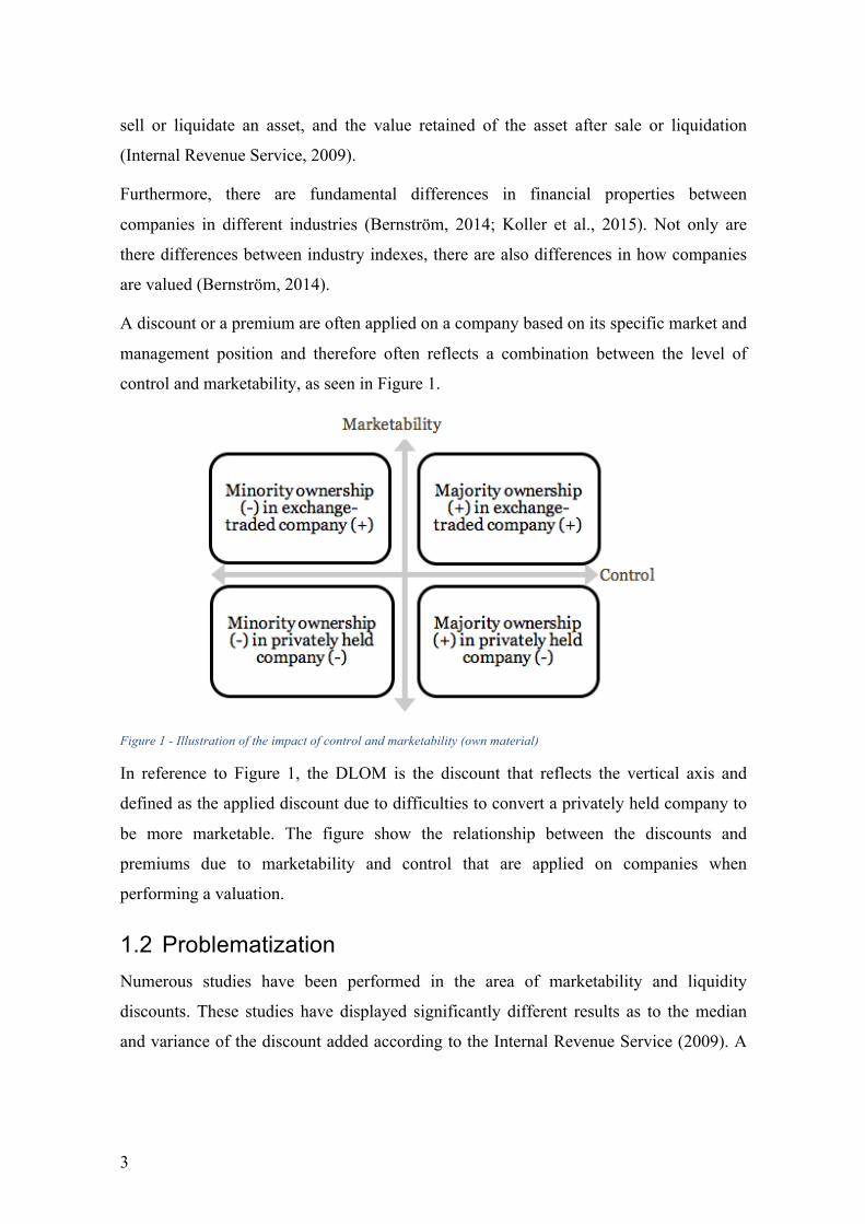
A discount or a premium are often applied on a company based on its specific market and

management position and therefore often reflects a combination between the level of

control and marketability, as seen in Figure 1.

Figure 1 - Illustration of the impact of control and marketability (own material)

In reference to Figure 1, the DLOM is the discount that reflects the vertical axis and

defined as the applied discount due to difficulties to convert a privately held company to

be more marketable. The figure show the relationship between the discounts and

premiums due to marketability and control that are applied on companies when

performing a valuation.

1.2 Problematization Numerous studies have been performed in the area of marketability and liquidity

discounts. These studies have displayed significantly different results as to the median

and variance of the discount added according to the Internal Revenue Service (2009). A

4

majority of these studies are theoretically based and has little empirical foundation (Pratt

& Niculita, 2008; Internal Revenue Service, 2009).

Previous research and a majority of commonly accredited studies on the DLOM have

been based on U.S. market data between 1970 and early 2000s (Pratt, 2001). As such, it

is a potential cause for concern as the U.S. stock markets differ from the European in

both regulatory aspects as well as in liquidity. In addition, the properties and structure of

the markets have changed during the last decades.

Furthermore, none of the most commonly referred models consider variations in

marketability that could appear in specific industries. This means that companies with

completely different properties, markets, and macroeconomic outlooks are valued the

same way. All these factors affect the prerequisites for the DLOM, and thus makes it

interesting to study further how the DLOM varies based on industries, as well as adding a

focus towards the European market, and making comparisons between the European and

the U.S. market.

1.3 Purpose The purpose of this thesis is to empirically investigate and identify how potential lack of

marketability affects business value for companies registered in Europe. Furthermore,

industry-specific aspects and explanatory factors will be investigated and tested for a

number of major industry groups.

1.4 Research questions The purpose leads to two research questions, which answers could provide a foundation

for further development of models for determining DLOM in Europe.

Research Question 1:

How much does the marketability discount differ in value between European registered

companies and US equivalents?

Research Question 2:

To what extent, and what are the explanatory factors of the marketability discount

between major industry groups in Europe?

5

1.5 Delimitations The study focus on the discounts for lack of marketability, and does not investigate

discounts for lack of control. In reference to the model on impact of control and

marketability (figure 1) the study focuses on the vertical dimension and does not include

the horizontal dimension that involves discounts and premiums related to control. This

limitation was due the hardship of finding readily available combined data on both

marketability and control. The study is merely focused on the European and the US

market, and companies registered in these markets. Delimitations regarding investigated

industries and data is presented in chapter five.

1.6 Expected contribution The thesis intends to contribute to an increased understanding and the accuracy of the

application of DLOM. The results can be supportive in the development of future

valuation models, and for improving the accuracy while applying the discount on

valuations of unlisted European companies. Furthermore, the thesis intends to showcase

differences in valuation of marketability between regional markets, industries and over

time. The setup of the methodology used in the thesis intends to contribute to the

research field and academia in providing knowledge on valuation adjustments.

6

1.7 Disposition Chapter one leads to a problem formulation, the purpose, and subsequently to the

research questions. The chapter is intended to give the reader a background to the subject

and an understanding why the subject should be researched.

Chapter two presents and argue around the chosen theoretical framework on which the

thesis is based as well as a literature review and previous studies. This frames the context

in which the thesis is formulated, e.g. which economic assumptions and broader

theories/frameworks that are needed to understand the concept of marketability on

corporate value. The chapter puts DLOM into a wider context of valuation, and reviews

commonly encountered methods for determining it. It also contains a review of previous

applications of DLOM in legal cases.

In chapter three, the method and the research design is presented, along with arguments

explaining why the chosen method is suitable and accurate for determining DLOM. It

explains in detail how the data is processed and analyzed, and what data models that are

formulated. In addition, measures to achieve high validity, reliability and generalizability

are explained here.

Chapter four contains a thorough review of the data, including its sources and collection,

content, accuracy, and delimitations. Data is summarized in tables and graphs to increase

and support the understanding of the following analyses.

The results of the regression analyses and other conducted analyses are displayed in

chapter five.

The results as well as methods for analyses are discussed in chapter six. A focus is put on

the understanding and interpretation of the results and the conducted analyses. These are

then further outlined with conclusions in chapter seven.

The thesis is finalized with a section on more practical and managerial implications of

the results, a critical perspective to the findings of the study, and suggestions for future

research

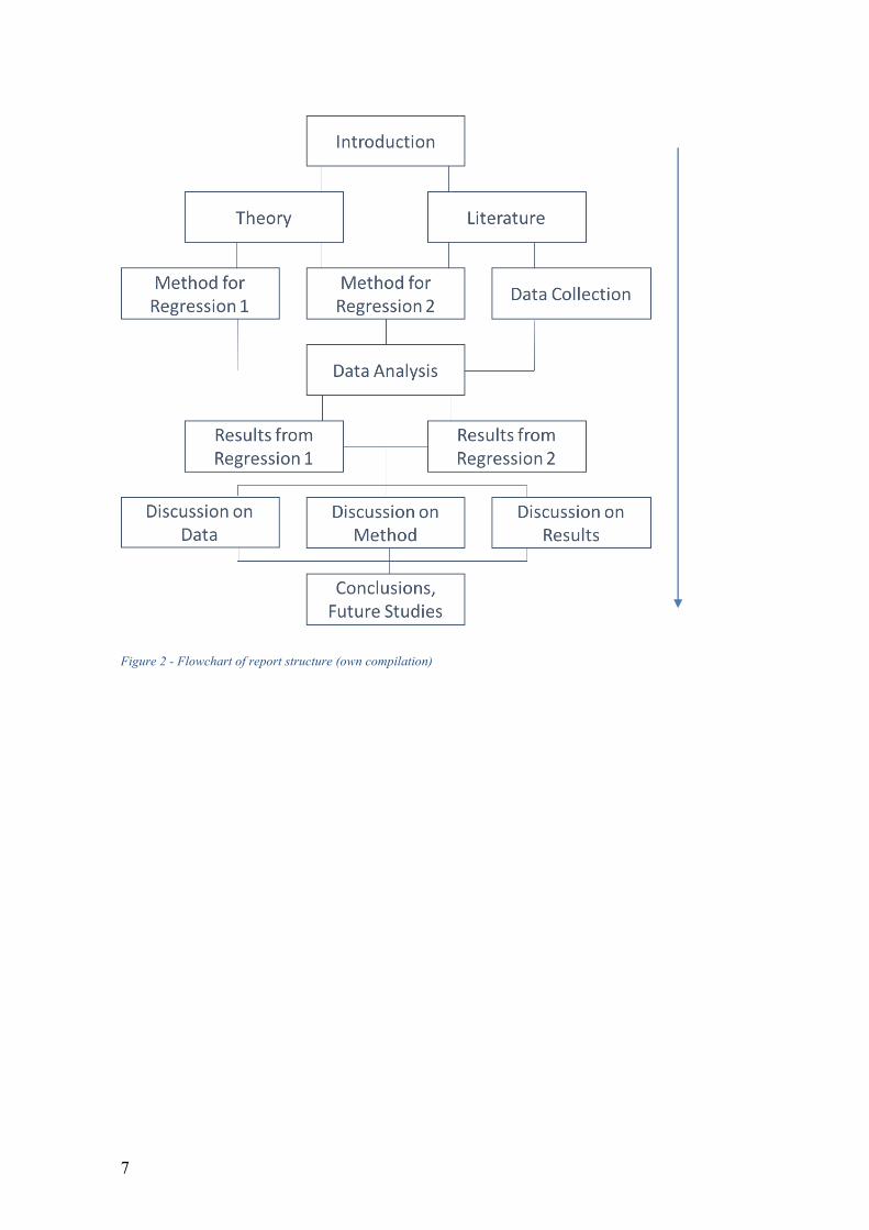
The outline of the report is displayed in the flowchart in Figure 2.

7

Figure 2 - Flowchart of report structure (own compilation)

8

2 Literature and Theory This chapter consists of the theoretical framework on which the empirical analysis is founded. It sets the context for the research and explains the fundamental financial and economic models presupposed to be guidance for the study. It also links together modern valuation techniques with the theoretical framework. It continues with an investigation towards previous research within the field of marketability, containing models and factors that research has found adequate to explain DLOM, as well as examples of its applications.

2.1 Efficient Market Hypothesis In order to understand why marketability affects company value, several theoretical

assumptions have to be made. These are based on early economic theories, that builds the

foundation for modern market theory. In 1900, Louis Bachelier suggested that all stock

movements can be attributed to two factors: Mathematical effects, as a result of games of

chance, and probabilities based on future events, which thus cannot be determined in

mathematical models (Bachelier, 1900). He introduced a paradox, saying that “While the

market neither believes in a rise nor in the true price, some movements […] may be more

or less probable.” This can be seen as the foundation to the more recent theories

regarding movements in share prices only being attributable to new available information

such as the Efficient Market Hypothesis (EMH) (Jensen, 1978).

The EMH is a set of conditions and assumptions formulated by Eugene Fama in 1970

(Fama, 1970). The hypothesis can be summarized as the notion that security prices fully

reflect all available information (Fama, 1991). However, there are several levels of the

EMH (Fama, 1970). The weak form implies that the information set consist of historical

asset prices. Furthermore, the semi-strong form states that only the information that is

publicly available is considered. Finally, the strong form also takes into consideration

private information for certain investors. The weak form has since coining been altered to

take into consideration only information in which marginal costs of gathering the

information is less than the potential gain from holding the information (Jensen, 1978).

The paradigm of the EMH can be extended into two assumptions. First, it implies that the

only thing that could cause a movement of a share price is the introduction of new

information. Second, it implies that an over- or undervaluation of a share would motivate

investors to make decisions, ultimately leading to an equilibrium equal to the real value

of the share. This means that, assuming information symmetry, the prices of securities

9

accurately would reflect the present value of all future free cash flows which the security

holder can claim.

While the weak form of EMH has gained traction in all aspects of financial economics,

there are several instances of inconsistencies. One example of such inconsistency is the

observed “January effect”. A commonly cited study consisted of market data from 1904

to 1974, where Rozeff and Kinney (1976) found that the average returns of securities in

January made up one-third of the total annual returns for that security (Loewenstein &

Thaler, 1989). This is an indication that the EMH does not fully explain market

movements, and further research into behavioral finance is required for deeper

understanding into market reactions.

As a result of information technology development lately, most equity markets can be

reached from anywhere in the world, making virtually all capital markets global.

According to the strong EMH, this would imply that all markets have the same

characteristics, which is not true (Fama, 1991). Therefore, the market differences must be

attributed to personal biases or technical effects. It can be argued that information

asymmetry and a preference to home markets leads to investors not being fully

globalized (Subrahmanyam & Titman, 1999).

However, as information technology develops, the information distribution should as

well (Subrahmanyam & Titman, 1999). This leads to markets becoming more efficient as

more investors have access to the same information and the cost of transactions (even

from across the world) decreases (Fama, 1991). With more efficient markets, profiting

becomes more difficult, and this is a trend that can be seen in the development of Initial

Public Offering (IPO) first-day profitability. It has, in line with theory, decreased steadily

over the years (Ritter & Welch, 2002).

2.2 Value In order to understand how certain companies are subject to discounts and premiums, a

thorough understanding of the fundamentals of value is required. In short, value can be

attributed to three factors: growth, profitability and risk (Bernström, 2014; Koller et al.,

2015). However, these three factors are considered differently depending on the context

in which value is analyzed. There are several definitions of value, depending on

geographical settings and purpose of valuation (Pratt & Niculita, 2008).

10

2.2.1 Fair Market Value Following the frameworks of the EMH, the related definition of value is the Fair Market

Value (FMV). More specifically, it resembles the adjusted weak form of EMH as it

assumes that both the buyer and seller of a security has reasonable access to information

(Gordon, 1952; Pratt & Niculita, 2008). A commonly used definition for FMV is that it

resembles the value of an asset for all investors, regardless of individual synergic effects

for certain investors, and assumes that all investors have reasonable access to the same

set of information.

2.2.2 Other definitions on value The definition of Investment Value (IV) represents what value an investment in an asset

could have for a specific investor (Pratt & Niculita, 2008). Reasons why it could differ

from the FMV are, for instance, differences in perceptions of risk and return, growth

estimates as well as potential synergies with the investor’s current assets. For valuation

purposes, it is more difficult to implement than the FMV.

Another definition of value is the Fair Value (FV), which varies depending on context

(Pratt & Niculita, 2008). In business valuation for market purposes, it is sometimes

referred to as the value of shares immediately before any corporate action to which the

shareholder objects. For reporting purposes however, it is referred to as the fair market

value in the most beneficial market for the asset or security.

2.2.3 Appraising value In order to understand how the discounts and premiums are added, the unadjusted value

of the company has to be determined. This can be done in three general ways: the income

approach, the market approach and the asset approach (Bernström, 2014). The income

approach is used to value the company with consideration to all three fundamental factors

of value (Koller et al., 2015). It is often realized through the Discounted Cash Flow

Model (DCF), in which several assumptions and the model are based on the EMH. For

instance, the model assumes that there only is one share value, based on the cost of

capital and all future cash flows of the company to which the shares belong. The cost of

capital is often calculated as the weighted average of the cost of debt and equity, where

the cost of equity most commonly is appraised using the Capital Asset Pricing Model

11

(CAPM). This model determines the capital cost through the risk-free rate, a market risk

premium and a company-specific measure of risk called beta (Koller et al., 2015).

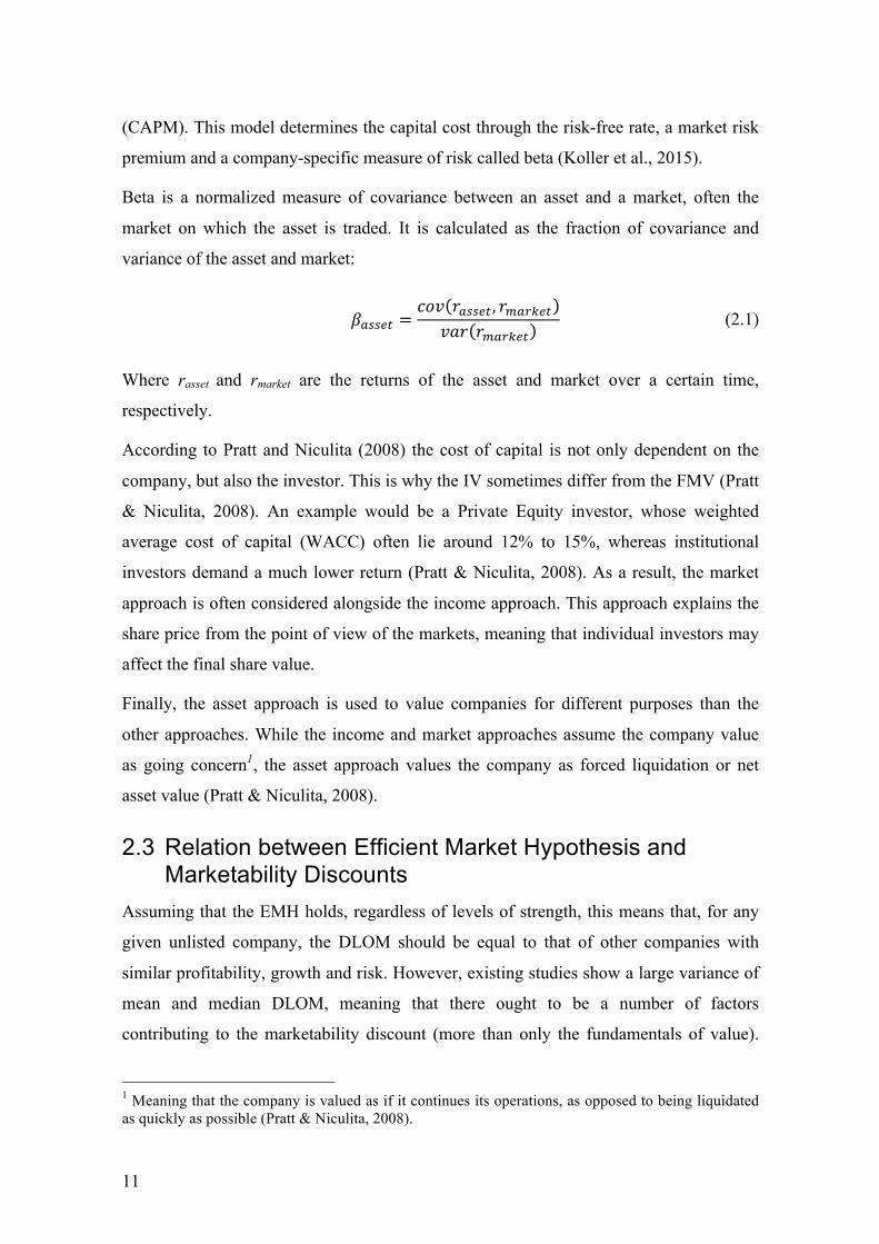
Beta is a normalized measure of covariance between an asset and a market, often the

market on which the asset is traded. It is calculated as the fraction of covariance and

variance of the asset and market:

!"##$% =

'() *"##$%, *,"-.$%)/* *,"-.$%

(2.1)

Where rasset and rmarket are the returns of the asset and market over a certain time,

respectively.

According to Pratt and Niculita (2008) the cost of capital is not only dependent on the

company, but also the investor. This is why the IV sometimes differ from the FMV (Pratt

& Niculita, 2008). An example would be a Private Equity investor, whose weighted

average cost of capital (WACC) often lie around 12% to 15%, whereas institutional

investors demand a much lower return (Pratt & Niculita, 2008). As a result, the market

approach is often considered alongside the income approach. This approach explains the

share price from the point of view of the markets, meaning that individual investors may

affect the final share value.

Finally, the asset approach is used to value companies for different purposes than the

other approaches. While the income and market approaches assume the company value

as going concern1, the asset approach values the company as forced liquidation or net

asset value (Pratt & Niculita, 2008).

2.3 Relation between Efficient Market Hypothesis and Marketability Discounts

Assuming that the EMH holds, regardless of levels of strength, this means that, for any

given unlisted company, the DLOM should be equal to that of other companies with

similar profitability, growth and risk. However, existing studies show a large variance of

mean and median DLOM, meaning that there ought to be a number of factors

contributing to the marketability discount (more than only the fundamentals of value).

1 Meaning that the company is valued as if it continues its operations, as opposed to being liquidated as quickly as possible (Pratt & Niculita, 2008).

12

Using this framework, the theory is formed that there are factors affecting DLOM, and

that there should be a possibility to derive these factors from historical market data.

In a perfect capital markets setting2, an asset can be liquidated to cash at the fair market

price according to the present value of all future free cash flows (Bajaj et al., 2001;

Koller et al., 2015). However, due to market imperfections, this setting is far from the

truth and there are substantial effects on the calculated value due to transaction costs,

taxes and less than perfect liquidity (Jensen, 1978). This implies that the variance of

marketability could be seen as an indicator that the markets are neither efficient nor

perfect.

2.4 Marketability and Liquidity The consideration of marketability is not without controversy (Bajaj et al., 2001). In

some jurisdictions, it is believed that marketability does not promote fair value, and is

thus never applied in legal settings (Laro & Pratt, 2005). In other areas, it is considered a

necessity for valuation of privately held companies.

Among tax professionals, marketability indicates the “salability” of a company, solely

taking into consideration whether or not a company can be sold or bought by certain

interests (Internal Revenue Service, 2009). In financial settings regarding business

valuation however, marketability is defined as “the ability to convert the business

ownership interest (at whatever ownership level) to cash quickly, with minimum cost in

doing so and with a high degree of certainty of realizing the expected amount of net

proceeds” (Pratt & Niculita, 2000). This is similar to the definition by the International

Glossary of Business Valuation Terms which states that marketability is internationally

used as the ability to quickly convert property to cash at minimal cost (AICPA, 2011).

Bajaj et al. (2001) adds that marketability implies salability without price concessions.

Within business appraisal professionals, the rule of thumb for marketability is whether or

not the asset or security is convertible to cash in three business days (Mercer, 2001; Laro

& Pratt, 2005). According to Mercer (2001), this is binary, meaning that an asset either is

marketable or not. While this definition primary holds for privately held companies,

public counterparts experience a similar notion that the market is adequately active for an

asset to achieve liquidity in three days. Contrary to the definition however, marketability

2 Implying that there are no costs associated with transactions, no taxes nor any trade restrictions.

13

is not a black-or-white subject (Laro & Pratt, 2005). For instance, one factor that affects

marketability in privately held companies is the frequency of private transactions of

company stock, which could attain a large range of values and is thus not binary.

While the terms of liquidity and marketability often are used interchangeably, there are

some differences in definitions and applications (Reilly & Rotkowski, 2007). According

to IRS (2009), marketability indicates the fact of salability while liquidity indicates how

fast the sale can occur with preserved value. Pratt & Niculita (2008) defines the

difference as “marketability focusing on finding the appropriate market, […] and

liquidity focusing on realizing cash proceeds.”

While marketability itself is an important aspect in valuation, the combination of

marketability and control is more so. Together, they create a four-sided matrix, in where

marketable control in a company is the most valuable, and nonmarketable minority

interests are the least. This is visualized in Figure 1. Worth noting is that neither of the

two parameters are binary; there is an almost continuous spectrum of levels of

marketability, as it is time dependent and company specific. Control is more stepwise, as

it could imply total ownership, majority, being the largest shareholder or holding a

minority share.

2.4.1 Factors affecting marketability The reasons why marketability causes a discount are few, as it is related to two things:

The time it takes to sell a non-marketable company, i.e. the time value of money, and the

price at which the non-marketable company can be sold (Pratt, 2001; Novak, 2016).

However, multiple factors have been identified that affect the magnitude of the discount.

Bajaj et al. (2001) identifies several factors in the previous literature that is expected to

affect marketability:

• The uncertainty of the asset’s value, due to the potentially high opportunity cost arising for investors

• The difficulty for an outsider to appraise the value of an asset, as it leads to higher risk for external investors

• The extent to which there are close substitutes to the assets, since the number of substitutes are related to the liquidity in the market

• The duration of restrictions on trade • The amount of the asset (the share of the company) that is being sold, as it is

more difficult to sell a large share of a company quickly

14

In conclusion, it can be seen that Bajaj et al. (2001) considers marketability to be the

effect of the time value of money and the longer time it takes to sell a privately held asset

as compared to a publicly traded equivalent. Furthermore, in the U.S jurisdiction, the

commonly cited case of Mandelbaum v. Commissioner (1995) identifies ten potential

factors related to marketability and the lack thereof (Internal Revenue Service, 2009):

• Value of subject corporation’s privately traded securities vs. its publicly traded securities

• An analysis of the corporation’s financial statements • Dividend yield, ability and history • Industry positioning, history and economic outlook • The corporation’s management • The degree of control transferred with the block of stock to be valued • Restriction on transferability of the stock • The holding period until an investor can realize a sufficient profit • The corporation’s redemption policy • The cost of an IPO on the stock being valued

In addition, the IRS (2009) identifies a number of further factors, some of which

mentioned here:

• Number of identifiable buyers • Earnings, revenue and financial ratios • Shareholder structure, holdings by insiders, institutions, independent directors • Expected holding period • Volatility of stock

A few of the factors from the different sources overlap, but many are unique to the study.

The variance of factors could be due to different legal settings and different purposes for

the marketability applications. Several of the factors can be found as exceptions to

theories regarding perfect capital markets.

While these factors influence the magnitude of the marketability discount, it is difficult to

derive why there is a discount in the first place. Subrahmanyam & Titman (1999)

attributes parts of the marketability discount to the number of investors with

serendipitously retrieved information on the company.

2.5 Discounts and premiums Discounts and premiums are some of the most disputed valuation subjects among

professionals (Pratt, 2001). If there are indications of a need to account for differences

15

between the theoretical value and the market value of an interest, an appropriate discount

or premium should be applied after the base value is defined. The discount or premium

however, has no meaning before the underlying value is applied and confirmed

(Bernström, 2014). In addition, there is a requirement in most legal applications of

marketability discounts to state the evidence and reasons behind the chosen discount or

premium (Laro & Pratt, 2005).

The adjustments can be added in two ways (Laro & Pratt, 2005). The first method

implies adding an entity-level discount related to all investors in the company. The

second method adds shareholder-level discounts which can be individualized for certain

shareholders based on their restrictions or marketability.

An entity-level discount is applied when the underlying cause of the lack of marketability

is related to the company in question, such as environmental liability, key persons or

ownership structure. An example of this application is found in the U.S. court case Estate

of Mitchell v. Commissioner (1997), in which the discount was applied to all shareholders

regardless of ownership stake.

Shareholder-level discount or premiums are instead added based on the value of control,

degree of control or degree of marketability for specific stock. This takes into

consideration the four levels of ownership mentioned in section 3.3, where control or

lack thereof affects how much the marketability impacts company value.

2.5.1 Discounts of lack of Marketability for controlling and non-controlling interests

According to Pratt & Niculita (2008), there are two large adjustments to be made towards

share value, where marketability is one. The other one is adjustment for control, or lack

thereof, often called minority discount (Damodaran, 2005). These two discounts are often

added in conjunction, where the product of the two discounts are applied to a valuation of

a company. The result is that it in many cases would be misguiding to only look at

marketability adjustments and not minority, or vice versa (Damodaran, 2005). This is the

reason why many valuation analysts make no adjustments when valuing majority stakes

in closely held stock; the implication is that the premium added for majority ownership

cancels out the discount for lack of marketability. This is a broad assumption, especially

16

since control premiums often range around 20% and marketability discounts often end up

around 30% to 40% (Pratt & Niculita, 2008).

Furthermore, control, or lack thereof, is not binary (Pratt & Niculita, 2008). It can range

from 100% ownership, to majority holdings, to controlling minority, to non-controlling

minority. In Sweden as example, there are several points in ownership level where there

are value-changing differences in control (Aktiebolagslag, 2005:551). At a 90%

ownership, the owner may force compulsory redemption of the rest of the shares. At two-

thirds, the owner has control over emption (meaning that the owner can decide which

shares have precedence to dividends, issues etc), rights issues and much more. Between

51% and 49%, the ownership transcends from majority to minority, which is the

difference between having full and not full decision making power. A 10% ownership

allows for request of additional general meetings and influence of the level of dividends

for the year.

2.6 Initial Public Offerings As a way to finance future growth with equity, the IPO is often a large stepping stone for

companies expecting high growth and stable income in the future (Ritter & Welch, 2002;

PwC, 2011). While there are numerous reasons for companies to perform an IPO, the

result is always an increased liquidity and volatility of equity. By going public, the

company owner facilitates a potential acquisition of the company to a higher price than

they would have received if it was private (Ritter & Welch, 2002). The IPO usually

consists of around 20% to 30% of the company shares, as this would have minimal

impact on the control structures in the company.

Performing an IPO is a long, expensive process. This is due to the large amount of

regulations formulated by the financial regulatory agencies in the respective country

(PwC, 2011). Almost all companies subject to an IPO have to modify their accounting

and reporting systems, as it is financially unviable to have such extensive systems in a

privately held company. As a result, companies often undergo IPOs after having reached

certain stages in their life cycles (Ritter & Welch, 2002).

The following explanation of the process of an IPO is derived from a guide written by

PwC called Roadmap for an IPO (PwC, 2011). The process begins with an appraisal of

the company in question, in where its value is determined by external analysts. Often,

17

more than one valuation is conducted in order to avoid bias from the valuators. The

responsible banks create a syndicate and use their combined financial leverage to pitch

the value to the company. After the initial pitch, a thorough analysis of the company,

board and management is then conducted in a due diligence investigation. The point of

this is to increase the transparency into the company, so that potential new shareholders

have access to all relevant information before investing.

The company will then be filing for its IPO, where the regulatory institution in the

country receives a statement with a large amount of historical financial statements, key

data, company overview and risk factors. This part of the process takes approximately

one month. Once this is approved, the new shares are often offered to certain institutional

investors, and the response from these usually determines the price range for the IPO. A

number of the shares will be allocated to these investors prior to being publicly traded.

This is due to the fact that the underwriting banks have discretion as to whom receives

shares, and to what price (Ritter & Welch, 2002).

To perform this drawn-out process, the banks charge a fee normally up to 7% of the

entire offering value. This implies that, while the marketable stock after the IPO is worth

more than before, theoretically there is at least a 7% discount that should be added to the

valuation premium between privately held and publicly traded companies, without taking

into consideration any time effects of value due to the lock-in of capital.

2.6.1 The effects of IPOs on business value Stemming from the numerous studies performed on marketability by using pre-IPO

transaction data, it is safe to say that going public has an effect on the business value

(Bajaj et al., 2001; Emory Sr, 2002). For instance, the Williamette Management

Associates (WMA) studies between 1998 and 2002 displayed a median DLOM of 36.1%

as well as a mean DLOM of 23.9% (Garland & Reilly, 2004). In addition to this, there is

strong evidence that companies tend to go public at a share price lower than its business

value, as there often are strong upwards movements of share price at the first few days of

trading (Garland & Reilly, 2004; Ljungqvist & Wilhelm, 2005).

Ljungqvist & Wilhelm (2005) attribute some of the post-IPO price movements to

idiosyncratic effects. Without going too deep into reasons as to why companies go public

or why the IPO share price tends to be below the fair market value, the interesting result

18

is how the fair market value (after the share price stabilizes) differs from the pre-IPO

valuation. Assuming little differences in control from the transaction, the main change of

value can be attributed to the marketability and liquidity of the corporate stock (Ritter &

Welch, 2002).

Subrahmanyam & Titman (1999) mentions that the benefits from going public are more

substantial in larger, more liquid markets. This is attributed to the fact that public

companies have a higher utility from serendipitous information, which is more

widespread in larger markets. Since this implies that certain investors have access to

information that others do not, the value of the company differs between investors. Thus,

the investor that values a company higher naturally have an advantage and a possibility

to utilize the information for profit.

2.7 Previously accredited studies for Discounts for Lack of Marketability

A number of different models have been formulated to evaluate the DLOM in companies

(Bajaj et al., 2001; Pratt & Niculita, 2008). Starting in the late 1960s, academics began

using empirical market data of U.S. transactions to determine the market values of the

discount. In the 1990s and shortly before, a new type of models appeared which were not

based on market data, but instead on theoretical transactions.

2.7.1 Restricted Stock studies Comparing restricted stock3 to unrestricted counterparts, Gelman studied transactions of

the two types of securities between 1968 and 1970 (Bajaj et al., 2001). The 89

transactions studied displayed a mean and median marketability discount of 33%. The

year after, Moroney (1973) published a study of 146 transactions displaying an average

discount of 35.6% and median 33%. However, Moroney proposed that a higher DLOM

could be rightfully applied due to benchmarked transactions. Following these, Trout

published in 1977 a study conducted between 1968 and 1972 concluding an average

discount at 33.5% for restricted stock (Trout, 1977).

3 Restricted stock is a common method during company transactions to prohibit key persons from liquidating their assets, causing a huge price change. It is almost exclusively occurring on the U.S. market, and virtually inexistent anywhere else as there are legal limitations elsewhere regarding trading restrictions.

19

Investigating transactions between 1980 and 1982, the Standard Research Consultants

conducted a study displaying a median discount of 45%, although ranging between 7%

and 91% showcasing the large variance in the subject (Reilly & Rotkowski, 2007).

Meanwhile, Hertzel & Smith (1993) studied transactions between 1980 and 1987,

returning average and median discounts of 20.1% and 13.5% respectively.

The results of the restricted stock studies show that there is a significant variation of

results based on sample selection and methodology. It can be argued that restricted stock

is a strong measure of marketability since it is strictly black and white; either the stock is

marketable or restricted with only duration of restriction as factor that could affect the

marketability discount. However, criticism from court cases claim that restricted stock

studies are misguiding for determining DLOM for privately held companies, as the

restricted stock has a readily available market once the restriction period ends (Novak,

2016).

2.7.2 Pre-IPO studies Another commonly encountered empirical analysis is the pre-IPO method. This method

begins with an investigation of the share price of a company directly after an IPO, i.e. the

fair market value of the stock (Bajaj et al., 2001; Internal Revenue Service, 2009). It

compares this value to the share price of the company deducted from a preceding

transaction, in which a substantial share of the company was bought or sold to a price

that could be seen as the pre-IPO FMV of the stock. The fundamental assumption on

which this method is based is that the only difference between a privately held and

publicly traded company is the marketability and liquidity (Bajaj et al., 2001).

There are three commonly cited studies of this kind: Emory studies, Valuation Advisors

study and Willamette Management Associates (WMA) Studies (Internal Revenue

Service, 2009). Each of the studies range over a long time, through multiple business

cycles and on wide markets. Results from the studies vary, and for instance, there is a

significantly lower DLOM in 1999 and 2001 that have been accredited several reasons:

• Few IPO and sale transactions, • The height of the dot-com “bubble” was during these years • A extraordinary first-day return during the period.

20

A positive argument for the method is that they are the only DLOM studies that include

transactions of shares in privately owned companies. This is especially useful in this

thesis as it is aimed towards investigating the discounts in privately held companies.

According to Reilly & Rotkowski (2007) however, there are unique factors in every

company that affects which specific DLOM method that is most applicable.

The longest (in terms of time between first and last study), most thorough studies among

these are the Emory studies (Internal Revenue Service, 2009). Ranging from 1980 to

2000 and covering 4,088 transactions, the minimum value for the discount is around 25%

with a median discount over all studies of 47% (Saunders, 2000; Novak, 2016).

However, the data showed that the discount increased by 0.15% to 0.20% for each day

that separated the valuation from the IPO showing that the length of the time period

variance affects the marketability strongly. The Emory studies excluded companies on

the following bases (Novak, 2016):

• Companies in a development stage (i.e. high growth) • Company with a history of real operating losses • Companies with an IPO price of less than $5 per share • Foreign (non-U.S.) companies • Banks, REITs and utilities.

The documented Valuation Advisors studies are based on more than 3,500 transactions

where a limit is set to a two-year timespan prior to the IPO (Novak, 2016). It is focused

on the time between transactions and IPOs, where the median discount from a 0-3-month

timespan is 21.5% and a 1-2-year timespan is 58.9%. In addition, the Valuation Advisors

divided the transactions based on the type of security. The three security classes included

in the study are stock, options and convertible preferred stock.

The WMA also conducted 18 pre-IPO studies between 1975 and 1997 (Internal Revenue

Service, 2009). The transactions incorporated in this study only includes holdings of

shares between 25% and 49%, to avoid changes in control (Laro & Pratt, 2005). While it

is not clear what exact discounts they returned, a conclusion could be drawn that pre-IPO

studies display a higher average discount than the restricted stock studies (Saunders,

2000). This could be explained by the fact that restricted stock transactions already have

an established public trading market, and the restriction time is significantly shorter than

the duration between the IPOs and precedent transactions.

21

Summarizing all pre-IPO studies, the mean differences between public and private

transactions varied from 25% to 60% depending on market and timing. The pre-IPO

studies are often considered more accurate than the restricted stock studies due to the

higher likelihood of finding similar benchmarking subjects to the company being

valuated (Pratt, 2001). They do, however, display larger variations due to time between

the transactions (Saunders, 2000; Pratt, 2001).

Common criticism towards the accuracy of the pre-IPO studies is the selection bias of

companies that undergo an IPO (Bajaj et al., 2001). More specifically, the criticism

implies that only successful companies in growth phases undergo IPOs, thus meaning

that comparison between transactions in different points in time is misleading as the

company value would increase whether an IPO is performed or not. In addition, critics

claim that there is a measurable hype in combination with the IPOs, where the IPO itself

drives a price inflation and thus affects the DLOM (Reilly & Rotkowski, 2007). This was

especially apparent during the dot-com bubble, where first-day returns of stock averaged

65% (Emory Sr, 2002).

2.7.3 Theoretical models Two types of theoretical models are used in previous studies, option pricing models and

DCF models (Mercer, 2001; Internal Revenue Service, 2009). The option pricing models

are based on the assumption that, if an investor holds restricted or non-marketable stock,

the theoretical value of an option to sell or buy that stock by the end of the restriction

period could qualify as the price for liquidating the restricted stock instantly (Chaffee III,

1993). This adds another factor to the model, namely the volatility of the stock analyzed.

The other theoretical models are based on the DCF model, where the difference between

free cash flow to firm and to shareholders is investigated.

Using theoretical prices of options through Black-Scholes-Merton models4, Chaffee III

(1993) concluded that the price of European put option, with strike price equal to the

share price on the valuation date, and maturity date as far ahead as the restriction period

lasts, accurately represents the DLOM for the underlying stock (Reilly & Rotkowski,

2007). With volatility between 60% and 90% and a holding period of two years, the

4 The Black-Scholes-Merton model is a set of equations that determines the value of an option as a function of underlying volatility, spot price, strike price, interest rate and time to maturity (Merton, 1976; Black & Scholes, 1973).

22

discount varied between 28% and 41% (Hall, 2009). This model is only appropriate to

use for determining DLOM if the holding period is short and the volatility of the

underlying stock is low (Elmore, 2017). The high volatility could be questioned, but

Chaffee III (1993) insisted that it should be higher than equivalent market-traded stock.

The argument for the put option model is that it is based on avoiding losses. Assuming

that an investor holds non-marketable stock and purchases an option to sell those shares

at the free market price, the buyer of the security has effectively bought the marketability

for the shares since the cost of the put option represents the DLOM (Pratt, 2009).

Using “Look-back” put options, Longstaff (1995) concluded that the value of

marketability is the payoff from an option on the maximum value of the security,

meaning that the price of the option is stochastic. A look-back option works such that a

holder may exercise his option at a fixed strike price, but according to the most beneficial

price that the underlying stock reached during the holding period (Elmore, 2017).

Assuming five-year holding periods and a volatility of 30%, the discounts from the

Longstaff study surpassed 65% (Hall, 2009). This level of discount is much higher than

other researchers, but can be explained by the long holding period. The method requires

perfect market knowledge, and can be used to derive an upper bound to the marketability

discount (Elmore, 2017). The argument as to why this type of option can be used to

determine DLOM is that, while a privately held company is non-marketable for a certain

time, it may increase in value, which is represented in the maximization of profit by the

option.

Another commonly encountered set of studies for DLOM are the LEAPS studies. A

Long-term Equity Anticipation Program (LEAP) is bought by an investor for hedging

against long-term stock decline (Novak, 2016). The LEAP is priced based on the

company size, company risk, latest year profit margin, return on equity and industry.

Therefore, this method assumes that the DLOM are based on the same factors since the

DLOM is the relative price of a LEAP versus its underlying stock. It has shown to return

a lower DLOM than most other studies and should, contrary to the Longstaff studies, be

seen as a lower limit to the application of DLOM for non-marketable stock (Pratt &

Niculita, 2008).

The most recent addition to the library of DLOM models is that of DCF models (Pratt &

Niculita, 2008). The Quantitative Marketability Discount Model (QMDM) estimates the

23

value of the marketability as the ratio between the valuation of a company using

Enterprise DCF (to all investors) and Shareholder DCF (to only shareholders) (Mercer &

Harms, 2015). The underlying assumption in this model is that the marketability discount

is not a valuation input, but rather a result of market efficiency. The difference in

variables between Enterprise DCF and Shareholder DCF is displayed in Table 1.

Table 1 – Differences in variables used in Enterprise DCF and Shareholder DCF. This showcases the increased complexity in determining a Shareholder DCF as opposed to the normally used Enterprise DCF (Mercer & Harms, 2015).

Enterprise DCF Shareholder DCF Forecast Period Range of expected holding periods Projected Interim Cash Flows Expected Distribution

Expected growth in Distribution Timing of the Distribution

Projected Terminal Value Growth in value over holding period Premium or discount to projected enterprise

value Discount Rate Range of required holding period return

Building from the CAPM to evaluate required return, the Tabak model uses market data

on the additional required return from investors to hold an illiquid asset to estimate the

DLOM (Novak, 2016). Likewise, the AECA model stems from CAPM and extends it by

one factor for business-specific risk to consider the volatility of economic profitability

for non-public companies as compared to the volatility of market returns.

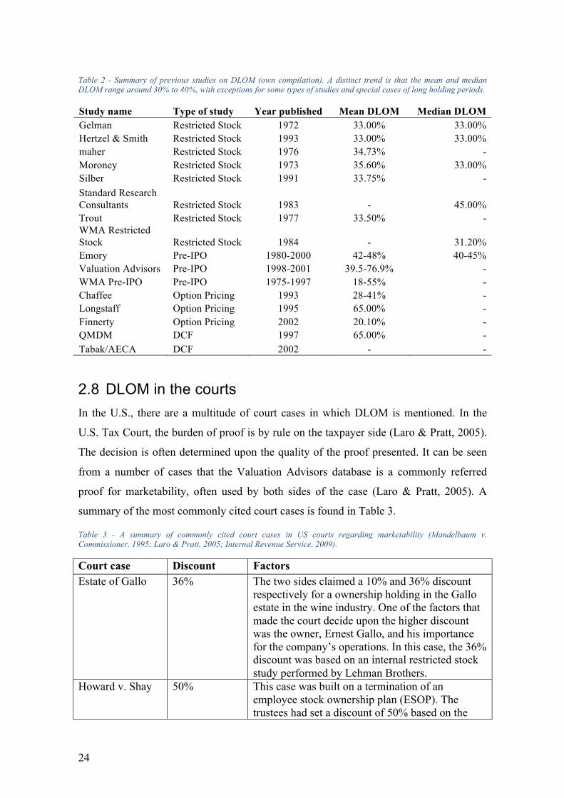
2.7.4 Summary of models The different models and their average discounts are summarized in Table 2. A

conclusion that can be drawn is that many of the models listed exhibit a mean or median

DLOM of between 30% and 40%. This result holds over several different determination

methods, with the only distinct exception being the DCF models. It can also be seen that

studies from different points in time return fairly similar means and medians. Another

observation is that there are large variations towards the DLOM from the pre-IPO studies

as well as the option pricing models, where the variations can be attributed to seasonal

effects in some cases (Emory Sr, 2002).

24

Table 2 - Summary of previous studies on DLOM (own compilation). A distinct trend is that the mean and median DLOM range around 30% to 40%, with exceptions for some types of studies and special cases of long holding periods.

Study name Type of study Year published Mean DLOM Median DLOM Gelman Restricted Stock 1972 33.00% 33.00% Hertzel & Smith Restricted Stock 1993 33.00% 33.00% maher Restricted Stock 1976 34.73% - Moroney Restricted Stock 1973 35.60% 33.00% Silber Restricted Stock 1991 33.75% - Standard Research Consultants Restricted Stock 1983 - 45.00% Trout Restricted Stock 1977 33.50% - WMA Restricted Stock Restricted Stock 1984 - 31.20% Emory Pre-IPO 1980-2000 42-48% 40-45% Valuation Advisors Pre-IPO 1998-2001 39.5-76.9% - WMA Pre-IPO Pre-IPO 1975-1997 18-55% - Chaffee Option Pricing 1993 28-41% - Longstaff Option Pricing 1995 65.00% - Finnerty Option Pricing 2002 20.10% - QMDM DCF 1997 65.00% - Tabak/AECA DCF 2002 - -

2.8 DLOM in the courts In the U.S., there are a multitude of court cases in which DLOM is mentioned. In the

U.S. Tax Court, the burden of proof is by rule on the taxpayer side (Laro & Pratt, 2005).

The decision is often determined upon the quality of the proof presented. It can be seen

from a number of cases that the Valuation Advisors database is a commonly referred

proof for marketability, often used by both sides of the case (Laro & Pratt, 2005). A

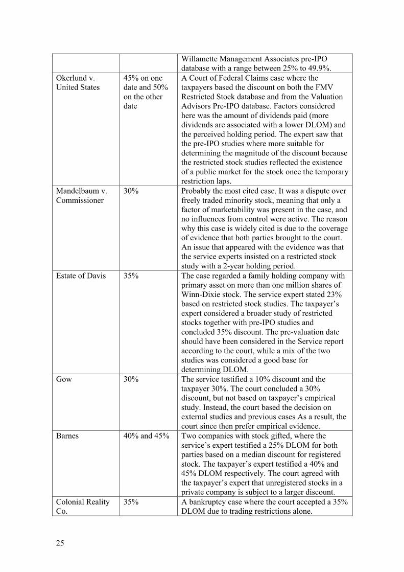
summary of the most commonly cited court cases is found in Table 3.

Table 3 - A summary of commonly cited court cases in US courts regarding marketability (Mandelbaum v. Commissioner, 1995; Laro & Pratt, 2005; Internal Revenue Service, 2009).

Court case Discount Factors Estate of Gallo 36% The two sides claimed a 10% and 36% discount

respectively for a ownership holding in the Gallo estate in the wine industry. One of the factors that made the court decide upon the higher discount was the owner, Ernest Gallo, and his importance for the company’s operations. In this case, the 36% discount was based on an internal restricted stock study performed by Lehman Brothers.

Howard v. Shay 50% This case was built on a termination of an employee stock ownership plan (ESOP). The trustees had set a discount of 50% based on the

25

Willamette Management Associates pre-IPO database with a range between 25% to 49.9%.

Okerlund v. United States

45% on one date and 50% on the other date

A Court of Federal Claims case where the taxpayers based the discount on both the FMV Restricted Stock database and from the Valuation Advisors Pre-IPO database. Factors considered here was the amount of dividends paid (more dividends are associated with a lower DLOM) and the perceived holding period. The expert saw that the pre-IPO studies where more suitable for determining the magnitude of the discount because the restricted stock studies reflected the existence of a public market for the stock once the temporary restriction laps.

Mandelbaum v. Commissioner

30% Probably the most cited case. It was a dispute over freely traded minority stock, meaning that only a factor of marketability was present in the case, and no influences from control were active. The reason why this case is widely cited is due to the coverage of evidence that both parties brought to the court. An issue that appeared with the evidence was that the service experts insisted on a restricted stock study with a 2-year holding period.

Estate of Davis 35% The case regarded a family holding company with primary asset on more than one million shares of Winn-Dixie stock. The service expert stated 23% based on restricted stock studies. The taxpayer’s expert considered a broader study of restricted stocks together with pre-IPO studies and concluded 35% discount. The pre-valuation date should have been considered in the Service report according to the court, while a mix of the two studies was considered a good base for determining DLOM.

Gow 30% The service testified a 10% discount and the taxpayer 30%. The court concluded a 30% discount, but not based on taxpayer’s empirical study. Instead, the court based the decision on external studies and previous cases As a result, the court since then prefer empirical evidence.

Barnes 40% and 45% Two companies with stock gifted, where the service’s expert testified a 25% DLOM for both parties based on a median discount for registered stock. The taxpayer’s expert testified a 40% and 45% DLOM respectively. The court agreed with the taxpayer’s expert that unregistered stocks in a private company is subject to a larger discount.

Colonial Reality Co.

35% A bankruptcy case where the court accepted a 35% DLOM due to trading restrictions alone.

26

The most commonly cited case is that of Mandelbaum v. Commissioner (1995) (Internal

Revenue Service, 2009). In this case, the foundation research was adequately covering to

allow the decision makers to form a model with ten factors that determined the DLOM,

to be used in future cases. The factors, mentioned in section 3.3.1, work as a guideline for

business appraisers to value a company with regards to marketability in legal disputes.

One of the reasons why the Mandelbaum case is widely cited is because it was a dispute

over freely traded minority interests, which means that the only issue was the lack of

marketability. Thus, no regard had to be taken towards control (Laro & Pratt, 2005).

Furthermore, Judge Laro mentioned that holding period was an important factor when

applying the DLOM, something that was overlooked in the previously cited studies. The

conclusion was that the restricted stock studies’ median of 35% DLOM and Pre-IPO

studies’ median of 45% was relevant, but the holding period was shorter than those in the

studies and thus the concluded DLOM was 30% (Mandelbaum v. Commissioner, 1995;

Laro & Pratt, 2005; Internal Revenue Service, 2009). A total of seven different restricted

stock studies and three pre-IPO studies were cited by the taxpayer’s expert. The criticism

against this evidence was that it only focused on a hypothetical willing buyer and seller.

A conclusion was that the stock in the case is “virtually illiquid” and an investor in the

company would have to wait 10 to 20 years for the investment to become liquid

(Mandelbaum v. Commissioner, 1995; Laro & Pratt, 2005).

Further reasons why the Mandelbaum case has received such attention is because it has

brought attention for the courts to consider the following:

• The court should expect detailed data developed by the experts, and not simply medians cited from previous studies

• There are potential reasons for the decision to go above or below the medians from previous studies due to financial factors

• One discount level does not apply to all companies • Case-specific analysis is required to form an opinion

Since then, many courts have required thorough analyses from both parties in all

valuation cases (Internal Revenue Service, 2009).

27

2.8.1 European juridical cases In the jurisdiction of the European Union (EU), there are few instances of issues with

marketability, and none of them are adequately significant to be published in law

journals. However, The European Group of Valuers’ Associations (TEGoVA) has issued

a framework of valuation standards which mentions marketability (TEGoVA, 2016).

However, it never mentions marketability of securities, only in relation to tangible and

intangible company assets.

2.9 Summary of theoretical assumptions This thesis assumes that there is a single value of DLOM for a company that perfectly

represents the marketability for that specific company, in that specific time. This is based

on the Law of One Price, which is a derivation of the EMH (Berk & DeMarzo, 2014).

Since there is a single value of DLOM, then that means that any reversible change in

marketability and liquidity has an equally reversible DLOM.

Furthermore, the FMV assumptions constitute that all potential investors have access to

the same information and knowledge, including that of DLOM. They also constitute that

all investors have the same required return for a specific asset, which is far from the

truth, especially in smaller companies. This does cause a difference in present value of

the cash flows, but taking into consideration every investor’s unique return requirement

would be near impossible in a financial model and thus a single WACC is used in the

valuation.

The reason why this thesis will be based on the paradigm of the FMV is that it would be

near impossible to formulate a general model for valuation taking into consideration

unique investor’s hidden values and incentives. The result of this delimitation is that the

value of the DLOM from this study may vary from the final transaction value, as an

investor with unique incentives may be inclined to pay more (or sell for less) than the

FMV. Since this definition of value is consistent with the financial models that are used

to value companies, it is also the definition most commonly used in equity research and

market valuation (Pratt & Niculita, 2008).

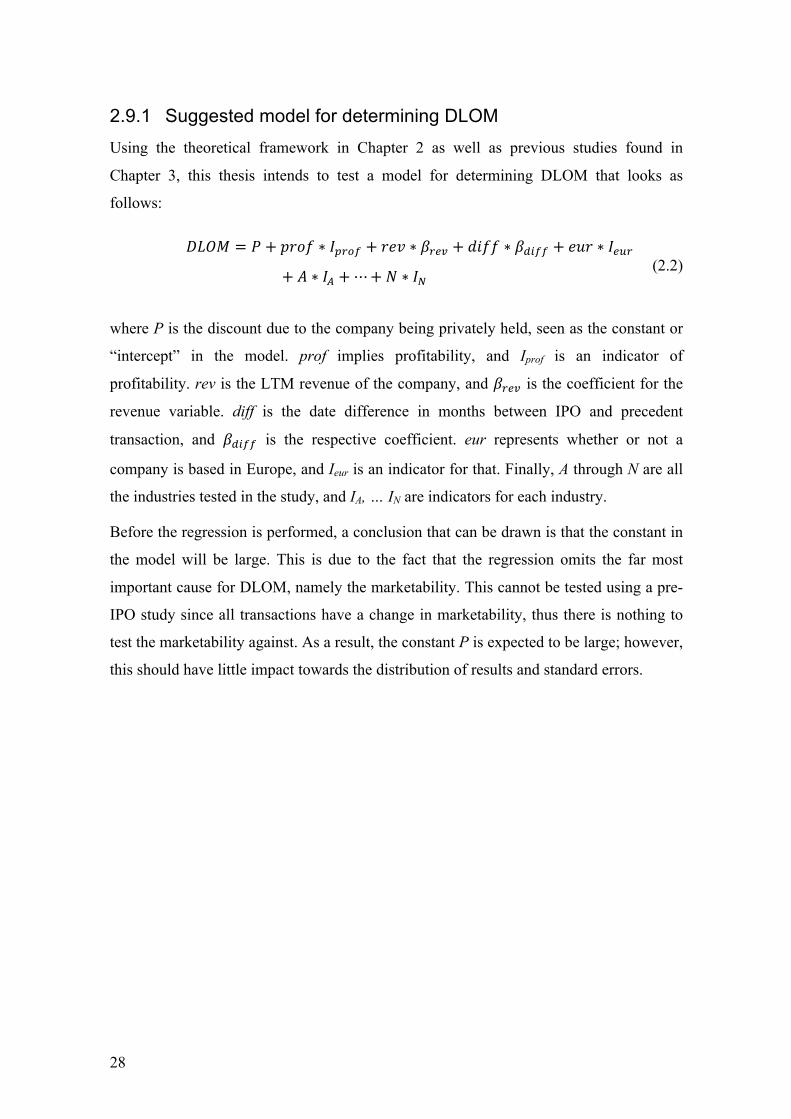
28

2.9.1 Suggested model for determining DLOM Using the theoretical framework in Chapter 2 as well as previous studies found in

Chapter 3, this thesis intends to test a model for determining DLOM that looks as

follows:

0123 = 4 + 6*(7 ∗ 9:-;< + *=) ∗ !-$> + ?@77 ∗ !AB<< + =C* ∗ 9$D-

+ E ∗ 9F + ⋯+ H ∗ 9I (2.2)

where P is the discount due to the company being privately held, seen as the constant or

“intercept” in the model. prof implies profitability, and Iprof is an indicator of

profitability. rev is the LTM revenue of the company, and !-$> is the coefficient for the

revenue variable. diff is the date difference in months between IPO and precedent

transaction, and !AB<< is the respective coefficient. eur represents whether or not a

company is based in Europe, and Ieur is an indicator for that. Finally, A through N are all

the industries tested in the study, and IA, … IN are indicators for each industry.

Before the regression is performed, a conclusion that can be drawn is that the constant in

the model will be large. This is due to the fact that the regression omits the far most

important cause for DLOM, namely the marketability. This cannot be tested using a pre-

IPO study since all transactions have a change in marketability, thus there is nothing to

test the marketability against. As a result, the constant P is expected to be large; however,

this should have little impact towards the distribution of results and standard errors.

29

3 Method This chapter explains the methodology behind the analysis conducted and how the model for DLOM used in the analysis is derived. Furthermore, it introduces the mathematical model that is used in the analysis, as well as the notation used throughout the report. This is followed by an explanation how the mathematical model will be used to answer the research questions.

3.1 Methodological approach and research design The chosen approach for the research is of an exploratory nature since it intends to find

patterns between different factors. In addition, the research approach is abductive. This

means that the research is based on an observation of an effect or event, and aims to find

the most direct explanation. The abductive approach is illustrated in the fact that the

study is aimed at looking for patterns in data rather than to prove or disprove hypotheses

(Collis & Hussey, 2013). The thesis follows a top-down approach, as it is founded on a

paradigm based on the EMH, which subsequently is expanded to the framework of

previously accredited studies. Since the result is expected to work as a guideline for

future reference, an inductive methodology is conducted (Collis & Hussey, 2013).

Furthermore, since the analysis will be of a statistical mathematical nature from a large

database, the analysis can be considered quantitative. This leads to a requirement for a

predetermined level of significance in the results. This structure of the thesis leads to

predictive results, meaning that the results ought to have an adequate significance level to

be applied elsewhere. In practice, this implies that the country- and geography-based

DLOM should be applicable to future valuations of unlisted companies.

The theoretical models that are used to analyze the raw data are based on an analysis of

previous literature on the subject. This implies that the focus of the thesis is not to invent

a new method for evaluating DLOM; rather, formulate a model to specify the DLOM

based on the findings of previous research.

3.1.1 Choice of quantitative method There are several potential ways to analyze the database quantitatively and retrieve

indications as to how the DLOM varies with factors (Novak, 2014). One such way is

performing a t-test, which is a method of hypothesis testing where the coefficient is

tested for a certain value (Montgomery et al., 2015). The difference between this method

and the multivariate regression model used is that the t-test allows for testing the

30

significance against other values than zeroes. However, the test requires an assumption

that the errors are normally and independently distributed, which is an assumption that

cannot be made for this investigation. Therefore, the Analysis of Variance (ANOVA) test

is more suitable for this study.

3.2 Literature collection The literature review has been conducted in order to cover the possible underlying

information needed to understand the nature of DLOM. The purpose of the review is to

understand precedent studies on the subject of DLOM, as well as give an overview on the

area of business valuation in order to further explain the problem formulation.

Numerous types of sources have been used for the information gathering. Some of the

information regarding valuation specifics (such as the DCF model) has been sourced

through course material in financing courses at The Royal Institute of Technology,

Stockholm (KTH), as these give a clear explanation and a head-first dive into the subject.

Information regarding the use of DLOM among valuation professionals, as well as legal

aspects, have been retrieved through the internal database of PwC Sweden, which

contains both academically accredited sources, as well as guidelines for valuation

analysts on addressing DLOM. Most previously accredited models for determining

DLOM, as well as the theoretical framework supporting the thesis, have been retrieved

through searches in the KTH Primo database and Google Scholar. These searches have,

among other, had keywords such as:

“DLOM”, “Discount for lack of marketability”, “Marketability discounts”, “Factors for

DLOM”, “DLOM models”, “DLOM in courts”, “pre-IPO”, “Valuation discounts”, etc.

3.3 Regression analysis As a commonly used method in econometrics to investigate the relations between

economic theory, statistics and mathematics, regression analysis is a basic and useful tool

to determine correlations. In order to test the significance of the resulting differences in

DLOM based on the factors found in the research questions, a regression analysis will be

conducted. In order to increase explanatory power of the regression, more factors than

the ones relevant to the research questions will be included. These factors are, among

other:

31

• Time difference between IPO and precedent transaction • Whether or not the company is profitable (positive net operating profit) at time of

IPO Using these factors in addition to those mentioned in the research questions as

independent variables, the regression will test their significance towards the dependent

variable DLOM for the specific company and transaction. This is conducted through

multivariate regression analysis, described generally in section 3.3.1. Primarily, the

regression analysis is conducted in Microsoft Excel through its function “Regression

analysis”. However, if this program is deemed inadequate to capture all the factors, errors

and outcomes, the dataset will be transferred to R Studio for further analysis.

As one of the most widely used techniques for analyzing quantitative data, linear

regression analysis uses relatively simple mathematical algorithms to explain connections

between variables through equations (Montgomery et al., 2015). It is used to approximate

the real connection between variables, using a sample or the full population of events.

However, despite using the full population of events, it is nearly impossible to fully

explain the relation between variables. In order to do so, all potential factors existing

have to be identified. Fortunately, the goal is rarely to achieve full explanatory power,

but rather adequately strong explanation to be able to draw conclusions towards the

connection between one variable and another.

3.3.1 Linear Regression model The following section is based on the literature of Montgomery et al. (2015).

There are five assumptions upon which a linear regression model is built:

• The dependent variable can be formulated as a linear function of independent variables

• Expected value of the error term is zero • The error terms have the same variance and are not correlated, which is translated

to homoscedasticity; this is investigated further below • Observations on the independent variable can be considered fixed in repeated

samples • The number of observations is greater than the number of independent variables

The multivariate linear regression model can be generalized, for every observation

(transaction), as:

32

J = !L + !MNM + !ONO + ⋯+ !.N. + P (3.1)

where β1, … βk are unknown constants representing regression coefficients for the

respective independent variable x1, …, xk. Furthermore, y represents the dependent

variable for each observation, β0 the intercept or “constant”, and ε the error term in the

observation (Montgomery et al., 2015).

The solution to the linear regression model is retrieved through the ordinary least-squares

method (OLS), which estimates the coefficients and the intercept such that the sum of

squares of the differences between the observations and the (multidimensional) straight

line is a minimum. This is achieved through a least-squares function:

Q !L, !M, … , !. = PBO = JB − !L − !TNBU

.

UVM

OW

BVM

(3.2)

where !T is the estimator to the j:th regression coefficient. This function S must be

minimized with respect to the different β. Thus, the least-squares estimators must satisfy

XQXY

= −2[\] + 2[\[Y = 0 (3.3)

or the standard form

[\[Y = [′]

(3.4)

which are the least-squares normal equations. Solving for !, the least-squares estimators

! of ! is

Y = [\[ `M[′] (3.5)

which is solvable if the regression variables x are linearly independent. This leads to the

vector of fitted values of the dependent variable corresponding to the observed values y

] = [Y = [ [\[ `M[′]

(3.6)

From here, the residual can be retrieved as

33

a = ] − ]

(3.7)

which is a vector with a value for each observation i.

Using this standard model for multivariate linear regression, the important resulting

information is the significance for a non-zero observation of the relationship between the

independent variables xi and the dependent y.

3.3.2 R-square The R2 statistic can be seen as a measure of goodness of fit. It resembles the explanatory

power of the regression, and thus is equal to the square of the correlation between the

dependent variable and the estimation of the independent variables and their coefficients.

This is defined as follows (Montgomery et al., 2015):

b/* J = b/* N! + b/* = (3.8)

From this, the R2 statistic can be defined as

cO =

b/* N!b/* J

= 1 −b/* =b/* J

(3.9)

Using the OLS framework described in the previous section, the R2 is maximized

(Montgomery et al., 2015). One way to interpret it is this: Assume that a R2 of 0.9 is

achieved. That means that 90% of variability in strength is accounted for by this

regression model (Montgomery et al., 2015). However, this is a statistic that easily can be

manipulated by adding more terms and more polynomials. For instance, if there are n

data points in a set of observations, then a polynomial regression with n-1 degrees would

return a perfect fit for the model, i.e. R2 =1.

The R2 is often low for cross-sectional data as this is seldom used to attempt to fully

attain explanatory power (Kennedy, 2011). For a descriptive research method to return

useful results however, it should be high. A low R2 may also indicate that the range of the

regression variable x was too small to adequately determine a relationship to the

dependent variable y (Montgomery et al., 2015).

34

3.3.3 Multicollinearity If two or more regression coefficients have no linear relationship whatsoever, they are

said to be orthogonal, meaning that the two variables have no interference (Kennedy,

2011; Montgomery et al., 2015). However, in most regression analyses, the variables are

not perfectly orthogonal. Multicollinearity is a common problem that appear when two or

more independent variables are perfectly or nearly linearly dependent (Montgomery et

al., 2015). Linear dependency occurs if there exists a set of constants tj such that

eUfU = 0W

UVL (3.10)

for the regression variables X1 … Xn.

This leads to several issues in the results from the OLS estimation. The most prominent

problem is that the estimation returns have unjustly high variances. The reason why this

occurs is as follows. Assume a model with two coefficients

J = !MNM + !ONO + P (3.11)

where !U and NU are the regression coefficients and variables respectively, and P is the

error term. The least squares normal equations for this model is

[\[ Y = [\] (3.12)

or

1 *MO*MO 1

!M!O

=*Mg*Og (3.13)

where r12 is the correlation between x1 and x2, and rjy is the correlation between xj and y.

Then, the regression coefficient estimators for this model is

!M =*Mg − *MO*Og1 − *MOO

!O =*Og − *MO*Mg1 − *MOO

(3.14)

35

respectively. Here we see that an increasing r12, due to higher correlation between

variables, lead to higher variances, namely

lim-kl→M

b/* !M → ∞ (3.15)

which shows that a high correlation between variables, and thus a high multicollinearity,

lead to high variances of coefficients.

Large violations regarding assumptions of nonexistent multicollinearity could lead to a

different sample returning completely different results and conclusions towards the

correlation. This can be detected in multiple ways. One way is to investigate if certain

variables with low t-statistics have a high collective F-statistic; if this is the case,

multicollinearity may be present. Another way is to display a correlation matrix, where

correlation coefficients between independent variables are shown. If these are high, there

is a risk for multicollinearity.

Usually, there are four sources of multicollinearity, shown in Table 4 (Montgomery et al.,

2015).

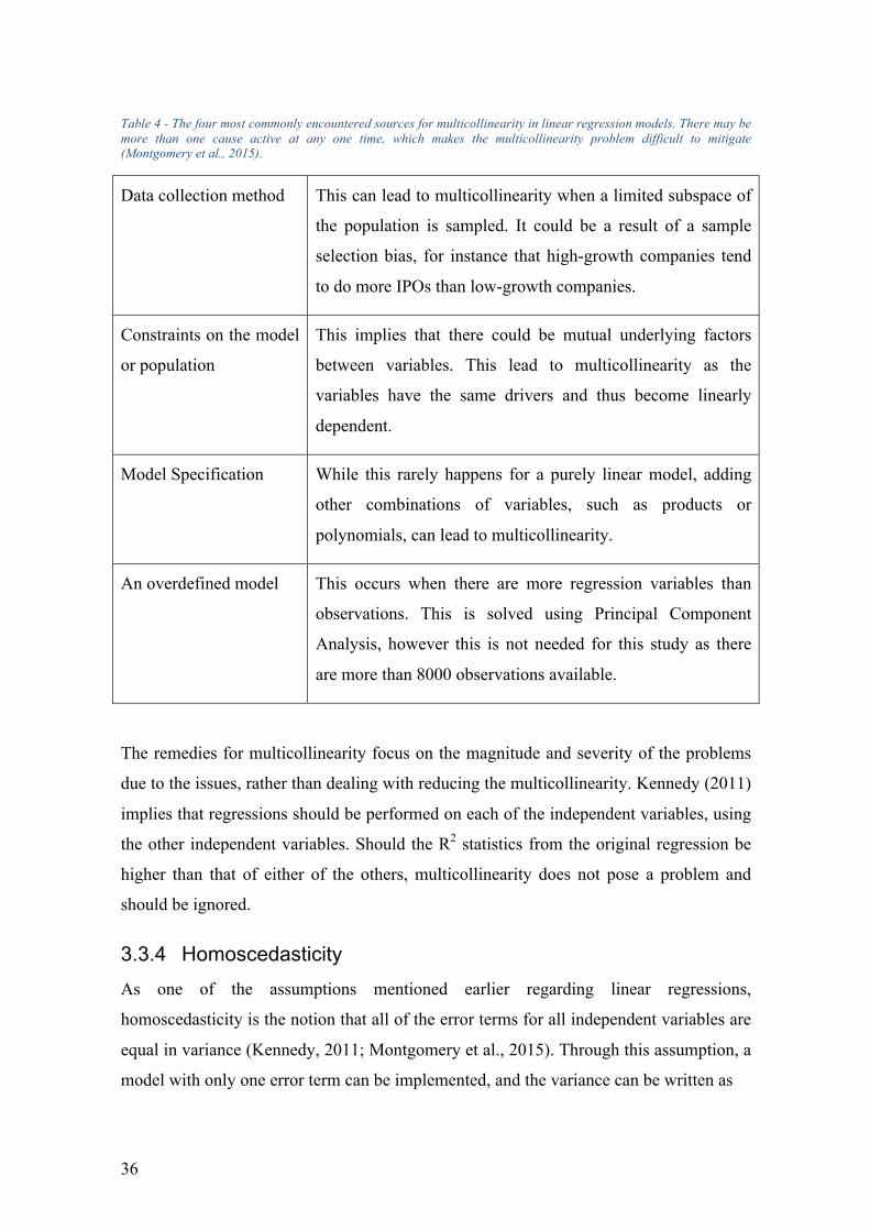
36

Table 4 - The four most commonly encountered sources for multicollinearity in linear regression models. There may be more than one cause active at any one time, which makes the multicollinearity problem difficult to mitigate (Montgomery et al., 2015).

Data collection method This can lead to multicollinearity when a limited subspace of

the population is sampled. It could be a result of a sample

selection bias, for instance that high-growth companies tend

to do more IPOs than low-growth companies.

Constraints on the model

or population

This implies that there could be mutual underlying factors

between variables. This lead to multicollinearity as the

variables have the same drivers and thus become linearly

dependent.

Model Specification While this rarely happens for a purely linear model, adding

other combinations of variables, such as products or

polynomials, can lead to multicollinearity.

An overdefined model This occurs when there are more regression variables than

observations. This is solved using Principal Component

Analysis, however this is not needed for this study as there

are more than 8000 observations available.

The remedies for multicollinearity focus on the magnitude and severity of the problems

due to the issues, rather than dealing with reducing the multicollinearity. Kennedy (2011)

implies that regressions should be performed on each of the independent variables, using

the other independent variables. Should the R2 statistics from the original regression be

higher than that of either of the others, multicollinearity does not pose a problem and

should be ignored.

3.3.4 Homoscedasticity As one of the assumptions mentioned earlier regarding linear regressions,

homoscedasticity is the notion that all of the error terms for all independent variables are

equal in variance (Kennedy, 2011; Montgomery et al., 2015). Through this assumption, a

model with only one error term can be implemented, and the variance can be written as

37

b/* = = oO (3.16)

where o is the standard deviation of the error e. A model misinterpreted as

homoscedastic leads to inconsistent variances of the estimates, and leads to an

invalidated F-test.

Heteroscedasticity is the occurrence of unequal variances between observations. It could

imply that the residual is linearly dependent with one of the independent variables

(Pindyck & Rubinfeld, 1998). An example would be that, for companies with larger

revenues, the sales are more volatile than in companies with smaller revenues, thus

leading to the larger ones returning larger residuals. The reason why this becomes an

issue is that, if some observations have larger residuals than others, then the sum-of-

squared residuals becomes larger and the ordinary least-squares estimation places more

weight on the observations with large error variances (Pindyck & Rubinfeld, 1998).

Because of this weighting, the OLS parameter estimators are still unbiased and

consistent, but they are not efficient. This means that the variances of the estimated

parameters are not the minimum variances.

One method to test for heteroscedasticity is called the Goldfeld-Quandt Test (Pindyck &

Rubinfeld, 1998). This test has the following algorithm:

1. Order the data by the magnitude of the independent variable X that is believed to

be dependent to the error variance

2. Omit the middle d observations, where d is a chosen number adequately large to

separate the top and bottom observations, and adequately small to allow for

enough degrees of freedom for the rest of the observations

3. Fit two separate regressions, one for the top and one for the bottom samples.

These regressions will thus have (H − ?)/2 pieces of data, where N is the total

number of observations, and [(H − ?)/2] − 2 degrees of freedom.

4. Calculate the residual sum of squares associated with each regression as ESS1 for

the low part and ESS2 for the high part.

5. Assume normally distributed error process, then the statistic ESS2/ESS1 will be F-

distributed with (H − ? − 4)/2 degrees of freedom. The null hypothesis that all

38

variances are equal can be rejected if the calculated statistic is greater than the

critical value of the F distribution for a given level of significance.

If the test deems that heteroscedasticity is present, then a correction has to be performed

(Pindyck & Rubinfeld, 1998). This can be done through using consistent estimates of

variances, called Heteroscedasticity-Consistent estimator (HCE). It is based on the

unbiased estimator

b/* ! =

NBOoBO

(NBO)O (3.17)

where the unknown variances oBO is replaced by the squares of the residuals PBO. Using

this method, the R2 of the regression will not change, however the estimates of standard

errors will change as they are now consistent estimates (Pindyck & Rubinfeld, 1998).

This still does not create efficient estimations; a weighted least-squares estimation

procedure has to be used instead.

3.3.5 P-value The p-value is a measure that equals the probability of obtaining a value outside the test

statistic. For instance, if the test is formulated in a way to test whether or not a statistic is

non-zero, the p-value explains the probability that a zero value (or a value of the opposite

sign) is returned. It is defined as follows for a normally distributed set of observations:

6 = 24 v > fL (3.18)

where P implies the probability, Z is the distribution of observations and X0 is the test

statistic. Z and X are in this case identically distributed.

3.3.6 F-test for joint null-hypothesis The F-test is a method for testing the null-hypothesis that a number of parameters !B all

are zero (Montgomery et al., 2015). Assuming normally distributed error terms, the F-

statistic looks as follows:

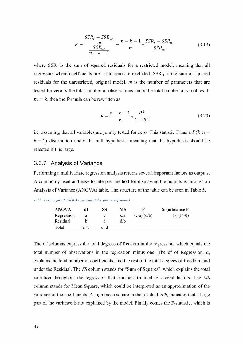
39

x =

QQc- − QQcD-y

QQcD-z − { − 1

=z − { − 1

y∗QQc- − QQcD-

QQcD- (3.19)

where SSRr is the sum of squared residuals for a restricted model, meaning that all

regressors where coefficients are set to zero are excluded, SSRur is the sum of squared

residuals for the unrestricted, original model. m is the number of parameters that are

tested for zero, n the total number of observations and k the total number of variables. If

y = {, then the formula can be rewritten as

x =

z − { − 1{

∗cO

1 − cO (3.20)

i.e. assuming that all variables are jointly tested for zero. This statistic F has a x({, z −

{ − 1) distribution under the null hypothesis, meaning that the hypothesis should be

rejected if F is large.

3.3.7 Analysis of Variance Performing a multivariate regression analysis returns several important factors as outputs.

A commonly used and easy to interpret method for displaying the outputs is through an

Analysis of Variance (ANOVA) table. The structure of the table can be seen in Table 5.

Table 5 - Example of ANOVA regression table (own compilation)

ANOVA df SS MS F Significance F Regression a c c/a (c/a)/(d/b) 1-p(F>0) Residual b d d/b

Total a+b c+d

The df columns express the total degrees of freedom in the regression, which equals the

total number of observations in the regression minus one. The df of Regression, a,

explains the total number of coefficients, and the rest of the total degrees of freedom land

under the Residual. The SS column stands for “Sum of Squares”, which explains the total

variation throughout the regression that can be attributed to several factors. The MS

column stands for Mean Square, which could be interpreted as an approximation of the

variance of the coefficients. A high mean square in the residual, d/b, indicates that a large

part of the variance is not explained by the model. Finally comes the F-statistic, which is

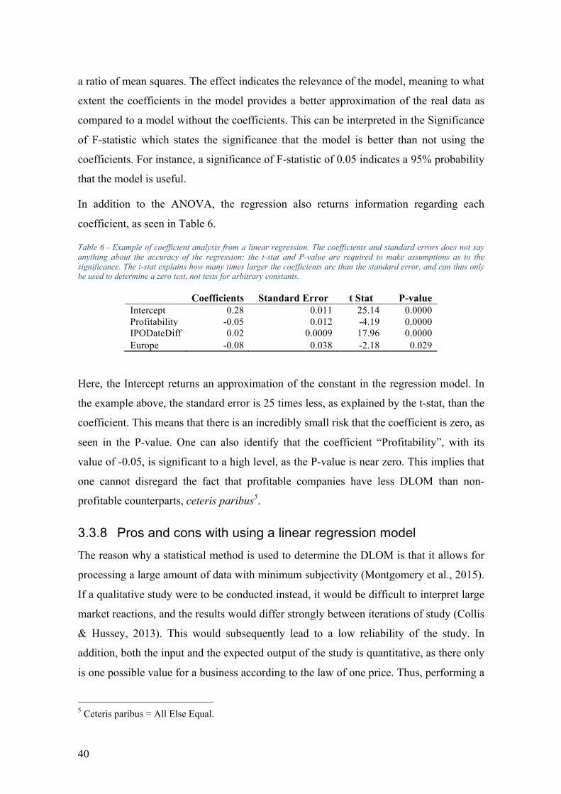
40

a ratio of mean squares. The effect indicates the relevance of the model, meaning to what

extent the coefficients in the model provides a better approximation of the real data as

compared to a model without the coefficients. This can be interpreted in the Significance

of F-statistic which states the significance that the model is better than not using the

coefficients. For instance, a significance of F-statistic of 0.05 indicates a 95% probability

that the model is useful.

In addition to the ANOVA, the regression also returns information regarding each

coefficient, as seen in Table 6.

Table 6 - Example of coefficient analysis from a linear regression. The coefficients and standard errors does not say anything about the accuracy of the regression; the t-stat and P-value are required to make assumptions as to the significance. The t-stat explains how many times larger the coefficients are than the standard error, and can thus only be used to determine a zero test, not tests for arbitrary constants.

Coefficients Standard Error t Stat P-value Intercept 0.28 0.011 25.14 0.0000 Profitability -0.05 0.012 -4.19 0.0000 IPODateDiff 0.02 0.0009 17.96 0.0000 Europe -0.08 0.038 -2.18 0.029

Here, the Intercept returns an approximation of the constant in the regression model. In

the example above, the standard error is 25 times less, as explained by the t-stat, than the

coefficient. This means that there is an incredibly small risk that the coefficient is zero, as

seen in the P-value. One can also identify that the coefficient “Profitability”, with its

value of -0.05, is significant to a high level, as the P-value is near zero. This implies that

one cannot disregard the fact that profitable companies have less DLOM than non-

profitable counterparts, ceteris paribus5.

3.3.8 Pros and cons with using a linear regression model The reason why a statistical method is used to determine the DLOM is that it allows for

processing a large amount of data with minimum subjectivity (Montgomery et al., 2015).

If a qualitative study were to be conducted instead, it would be difficult to interpret large

market reactions, and the results would differ strongly between iterations of study (Collis

& Hussey, 2013). This would subsequently lead to a low reliability of the study. In

addition, both the input and the expected output of the study is quantitative, as there only

is one possible value for a business according to the law of one price. Thus, performing a

5 Ceteris paribus = All Else Equal.

41

qualitative analysis would not only damage the reliability, but it would also be affected

by different interpretations of value and definitions of such.

A negative effect with the multivariate regression model is that it never returns an

absolute value of a correlation between variables. Instead, it shows indications and

confidence that there is a correlation, and thus the median or mean difference has to be

used instead in order to formulate a model. This is taken into consideration when

formulating the research questions, as the thesis intends to find connections between

DLOM and certain variables that could affect it.

3.4 Method for Research question 1 The method for answering research question 1 will be through a quantitative analysis,

followed by conclusions drawn from interpretation of the results. To recap, the question

is as follows:

How does the marketability discount differ in value between EU registered companies

and US equivalents?

3.4.1 Choice of variables In order to increase the explanatory power of the regression model, time difference and

profitability factors are included. These are chosen so that they together explain the value

of the company, meaning that they cover profitability, growth and risk. These three

factors are chosen since the profitability dummy explains the profitability factor of value,

and the time difference works as a proxy for growth and risk since those factors are time

dependent. Naturally, these two factors can by no means fully explain the value of the

transaction, since there are endless underlying factors. However, listing all potential

factors would be abundant and impossible with the time limitation of the thesis, and thus

the model is limited to these two.

3.4.2 Data processing and analysis In order to increase the accuracy of the regression and to mitigate the risk that the results

are skewed due to outliers, the data is processed. First, outliers are removed based on

guidelines found in previous pre-IPO studies on DLOM. All negative observations for

DLOM are removed, as these contradict all theoretical models and framework behind

marketability. The reasons, according to Emory (2002), for negative observations to

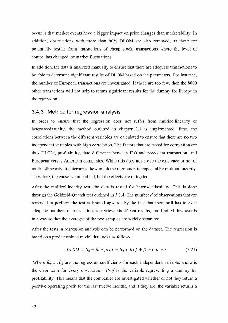
42

occur is that market events have a bigger impact on price changes than marketability. In

addition, observations with more than 90% DLOM are also removed, as these are

potentially results from transactions of cheap stock, transactions where the level of

control has changed, or market fluctuations.

In addition, the data is analyzed manually to ensure that there are adequate transactions to

be able to determine significant results of DLOM based on the parameters. For instance,

the number of European transactions are investigated. If these are too few, then the 8000

other transactions will not help to return significant results for the dummy for Europe in

the regression.

3.4.3 Method for regression analysis In order to ensure that the regression does not suffer from multicollinearity or

heteroscedasticity, the method outlined in chapter 3.3 is implemented. First, the

correlations between the different variables are calculated to ensure that there are no two

independent variables with high correlation. The factors that are tested for correlation are

thus DLOM, profitability, date difference between IPO and precedent transaction, and

European versus American companies. While this does not prove the existence or not of

multicollinearity, it determines how much the regression is impacted by multicollinearity.

Therefore, the cause is not tackled, but the effects are mitigated.

After the multicollinearity test, the data is tested for heteroscedasticity. This is done

through the Goldfeld-Quandt test outlined in 3.3.4. The number d of observations that are

removed to perform the test is limited upwards by the fact that there still has to exist

adequate numbers of transactions to retrieve significant results, and limited downwards

in a way so that the averages of the two samples are widely separated.

After the tests, a regression analysis can be performed on the dataset. The regression is

based on a predetermined model that looks as follows:

0123 = !L + !M ∗ 6*(7 + !O ∗ ?@77 + !| ∗ =C* + P (3.21)

Where !L, … , !| are the regression coefficients for each independent variable, and P is

the error term for every observation. Prof is the variable representing a dummy for

profitability. This means that the companies are investigated whether or not they return a

positive operating profit for the last twelve months, and if they are, the variable returns a

43

“1” as opposed to a zero. Diff is the variable representing the date difference between the

IPO and precedent transaction in months. Finally, EU is a dummy representing whether

or not a company is European or American.

3.4.4 Interpretation of results Performing a regression according to the model above gives us information regarding the

significance of the different variables towards DLOM. The most important outcome is

the significance, in p-value, of the coefficient !|. This explains what probability there is

that the coefficient could be zero, i.e. not relevant.

If there is a significant difference derived from the regression and the median for the

European companies is different from that of the American, this tells us that European

valuation analysts should look at EU data when determining DLOM rather than

American. The outputs and significance of the other independent variables can also be

used to further improve the accuracy of future DLOM calculations. However, the

relevance of these and theoretical foundation of such is not investigated in this thesis.

3.5 Method for Research Question 2 The method for answering research question 2 will, similarly to research question 1, be

through a quantitative analysis, followed by conclusions drawn from interpretation of the

results. The question is restated as follows:

To what extent, and what are the explanatory factors of the marketability discount


3.5.1 Choice of variables The same proxies for value as in the previous research question are chosen. The large

difference is how the industries are chosen to be tested. The companies will be sorted

according to their respective SIC major group6.

There are multiple ways to classify industries. Globally, the most commonly encountered

designation of industries is the Standard Industrial Classification (SIC) code index. This

6 SIC - Standard Industrial Classification - is an international system for classifying companies according to their industry belonging (U.S. S.E.C., 2015). For instance, any 2xxx and 3xxx code refers to manufacturing, the 37xx major group refers to transportation industry, and 3711 is Motor Vehicle and Passenger Car Bodies.

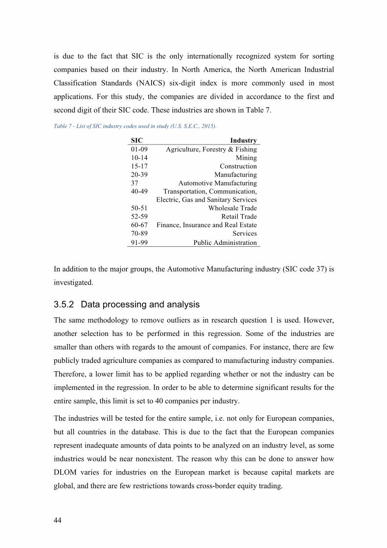
44

is due to the fact that SIC is the only internationally recognized system for sorting

companies based on their industry. In North America, the North American Industrial

Classification Standards (NAICS) six-digit index is more commonly used in most

applications. For this study, the companies are divided in accordance to the first and

second digit of their SIC code. These industries are shown in Table 7.

Table 7 - List of SIC industry codes used in study (U.S. S.E.C., 2015).

SIC Industry 01-09 Agriculture, Forestry & Fishing 10-14 Mining 15-17 Construction 20-39 Manufacturing 37 Automotive Manufacturing 40-49 Transportation, Communication,

Electric, Gas and Sanitary Services 50-51 Wholesale Trade 52-59 Retail Trade 60-67 Finance, Insurance and Real Estate 70-89 Services 91-99 Public Administration

In addition to the major groups, the Automotive Manufacturing industry (SIC code 37) is

investigated.

3.5.2 Data processing and analysis The same methodology to remove outliers as in research question 1 is used. However,

another selection has to be performed in this regression. Some of the industries are

smaller than others with regards to the amount of companies. For instance, there are few

publicly traded agriculture companies as compared to manufacturing industry companies.

Therefore, a lower limit has to be applied regarding whether or not the industry can be

implemented in the regression. In order to be able to determine significant results for the

entire sample, this limit is set to 40 companies per industry.

The industries will be tested for the entire sample, i.e. not only for European companies,

but all countries in the database. This is due to the fact that the European companies

represent inadequate amounts of data points to be analyzed on an industry level, as some

industries would be near nonexistent. The reason why this can be done to answer how

DLOM varies for industries on the European market is because capital markets are

global, and there are few restrictions towards cross-border equity trading.

45

3.5.3 Method for regression analysis The same two tests for multicollinearity and heteroscedasticity as in research question 1

are performed. The factors that are tested for correlation in the multicollinearity test are

thus DLOM, profitability, time difference, and each of the industries that are deemed

adequately large to be included in the regression. For the Goldfeldt-Quandt test, the same

limitations for the number d are implemented.

The regression model is predetermined as in research question 1. The difference here is

that region is not included, and is swapped for industries. Each industry selected for

testing will be assigned its own dummy variable, in which the industry receives a “1” and

all others a “0”. The model thus looks as follows:

0123 = !L + !M ∗ *=) + !O ∗ 6*(7 + !| ∗ ?@77 +!}∗ E +⋯+ !M| ∗ ~

(3.22)

where A, …, J are the industries deemed adequately large to remain in the analysis.

3.5.4 Interpretation of results The results of the regression explain whether or not there is any significance to

differences in DLOM between the different industries. By looking at the p-value for the

coefficients !} …!� to be zero, conclusions can be drawn as to how probable it is that the

industries have an impact on the DLOM for the companies.

Looking at the significance and the difference in median DLOM between the aggregated

database and the specific industries, it is possible to formulate a model for determining

the DLOM for that specific company. If there is a significant difference, then this could

indicate that the valuation analysts should take the industry into consideration when

applying a DLOM to a target company.

3.6 Summary of method For each research question, the method can be summarized in a few steps, with the

details described above.

46

First, a linear dependency model is formulated to be tested for significance. The

dependent variable DLOM is tested against two other variables, Profitability and Date

difference, as well as question-specific variables.

Second, the data is organized so that it contains the necessary information to be able to

determine the model. This includes removing unnecessary data such as company name,

date of IPO, operating profit and more.

Third, the data is analyzed to test whether it is adequate in order to draw conclusions.

This involves a correlation matrix between variables and testing the R2 of independent

variables. In addition, a Goldfeld-Quandt test is performed. If these tests pass, the data

can be determined to be homoscedastic and have no effects from multicollinearity, and

thus the regression can be performed.

Fourth, a regression analysis where the model is tested on all observations in the data set.

This is presented through an ANOVA table as well as a coefficient table, which together

holds adequate information regarding model fit and correlation in order to draw

conclusions regarding significance and correlation.

Fifth, for the independent variables that have proved to be significant, the median values

for DLOM for the different outcomes are calculated. This is the foundation for the final

model.

Sixth, a model is created using the significant variables retrieved above. It is presented as

a decision matrix, where the DLOM for a certain company can be derived from filling in

the different variables for that company.

47

4 Data collection This chapter showcases the database used in the model for DLOM. It explains the important parameters and how it will be utilized to derive factors for the marketability discount that subsequently is tested in the regression analysis. The removal of outliers and adjustments for skewed data is also explained in detail in the end of the chapter.

4.1 Gathering of data Gathering of the data is conducted through a thorough analysis of existing market

databases which potentially could be used to calculate a DLOM. Using the services of

Business Valuation Resources, an organization combining the knowledge and resources

of the leading valuation firms globally, a query shows that the database by Valuation

Advisors would be the most suitable for the thesis in question (Business Valuation

Resources, 2017).

The reason why the data exists is because, in most legal systems, a company has to

disclose all previous stock transactions in the prospectus prior to filing for an IPO

(Business Valuation Resources, 2017). In the instance of U.S. companies, the registration

is performed by the Securities Exchange Commission, which summarizes all transactions

in its EDGAR database. The Valuation Advisors then consult the EDGAR database once

an IPO has occurred, and decides whether or not the IPO and its precedent transaction is

fit for entry into the database. The database is updated at least once a month with new

transactions, which means that results may change over time.

The database does not contain every IPO. It excludes IPOs related to Real Estate

Investment Trusts (REITs), IPOs without precedent transactions in the stock, convertible

preferred stock or options prior to the IPO, as well as different types of funds and

partnership transactions. In addition, it does not contain every precedent transaction. For

every three-month period prior to the IPO, only the transaction with the highest price per

share, i.e. lowest implicit discount, is included.

Worth noting is that the database does not take into consideration cases of insider trading

and cheap stock. This is due to the fact that the SEC prospectus filing prior to the IPO

does not include this information. In cases of stock-based compensation programs where

the share prices often are deemed lower than their respective market value, the Valuation

Advisors adjust the prices of the shares to their FMV prior to implementation into the

database.

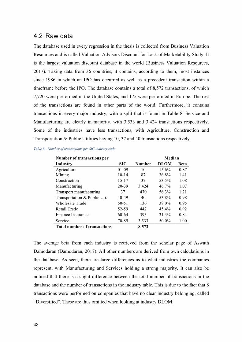
48

4.2 Raw data The database used in every regression in the thesis is collected from Business Valuation

Resources and is called Valuation Advisors Discount for Lack of Marketability Study. It

is the largest valuation discount database in the world (Business Valuation Resources,

2017). Taking data from 36 countries, it contains, according to them, most instances

since 1986 in which an IPO has occurred as well as a precedent transaction within a

timeframe before the IPO. The database contains a total of 8,572 transactions, of which

7,720 were performed in the United States, and 175 were performed in Europe. The rest

of the transactions are found in other parts of the world. Furthermore, it contains

transactions in every major industry, with a split that is found in Table 8. Service and

Manufacturing are clearly in majority, with 3,533 and 3,424 transactions respectively.

Some of the industries have less transactions, with Agriculture, Construction and

Transportation & Public Utilities having 10, 37 and 40 transactions respectively.

Table 8 - Number of transactions per SIC industry code

Number of transactions per

Median Industry SIC Number DLOM Beta Agriculture 01-09 10 15.6% 0.87 Mining 10-14 87 36.8% 1.41 Construction 15-17 37 53.5% 1.08 Manufacturing 20-39 3,424 46.7% 1.07 Transport manufacturing 37 470 56.3% 1.21 Transportation & Public Uti. 40-49 40 53.8% 0.98 Wholesale Trade 50-51 136 38.0% 0.95 Retail Trade 52-59 442 45.4% 0.92 Finance Insurance 60-64 393 31.3% 0.84 Service 70-89 3,533 50.0% 1.00 Total number of transactions

8,572

The average beta from each industry is retrieved from the scholar page of Aswath

Damodaran (Damodaran, 2017). All other numbers are derived from own calculations in

the database. As seen, there are large differences as to what industries the companies

represent, with Manufacturing and Services holding a strong majority. It can also be

noticed that there is a slight difference between the total number of transactions in the

database and the number of transactions in the industry table. This is due to the fact that 8

transactions were performed on companies that have no clear industry belonging, called

“Diversified”. These are thus omitted when looking at industry DLOM.

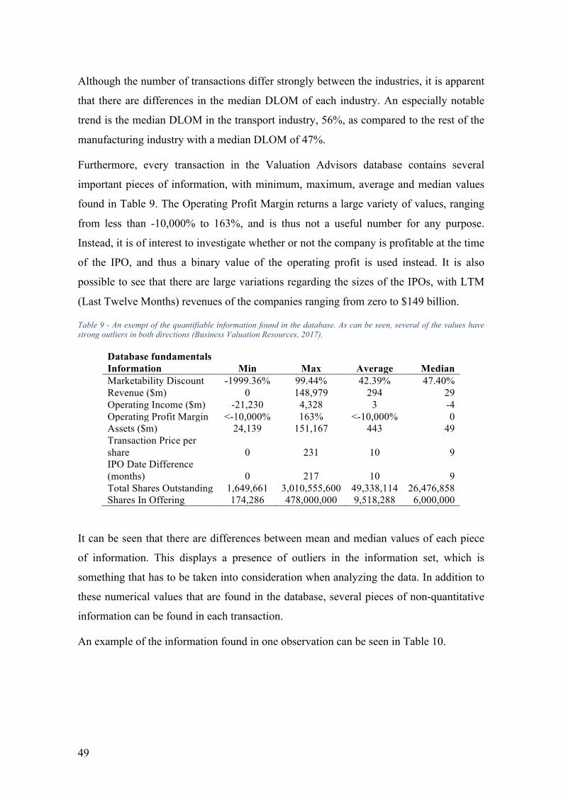
49

Although the number of transactions differ strongly between the industries, it is apparent

that there are differences in the median DLOM of each industry. An especially notable

trend is the median DLOM in the transport industry, 56%, as compared to the rest of the

manufacturing industry with a median DLOM of 47%.

Furthermore, every transaction in the Valuation Advisors database contains several

important pieces of information, with minimum, maximum, average and median values

found in Table 9. The Operating Profit Margin returns a large variety of values, ranging

from less than -10,000% to 163%, and is thus not a useful number for any purpose.

Instead, it is of interest to investigate whether or not the company is profitable at the time

of the IPO, and thus a binary value of the operating profit is used instead. It is also

possible to see that there are large variations regarding the sizes of the IPOs, with LTM

(Last Twelve Months) revenues of the companies ranging from zero to $149 billion.

Table 9 - An exempt of the quantifiable information found in the database. As can be seen, several of the values have strong outliers in both directions (Business Valuation Resources, 2017).

Database fundamentals Information Min Max Average Median

Marketability Discount -1999.36% 99.44% 42.39% 47.40% Revenue ($m) 0 148,979 294 29 Operating Income ($m) -21,230 4,328 3 -4 Operating Profit Margin <-10,000% 163% <-10,000% 0 Assets ($m) 24,139 151,167 443 49 Transaction Price per share 0 231 10 9 IPO Date Difference (months) 0 217 10 9 Total Shares Outstanding 1,649,661 3,010,555,600 49,338,114 26,476,858 Shares In Offering 174,286 478,000,000 9,518,288 6,000,000

It can be seen that there are differences between mean and median values of each piece

of information. This displays a presence of outliers in the information set, which is

something that has to be taken into consideration when analyzing the data. In addition to

these numerical values that are found in the database, several pieces of non-quantitative

information can be found in each transaction.

An example of the information found in one observation can be seen in Table 10.

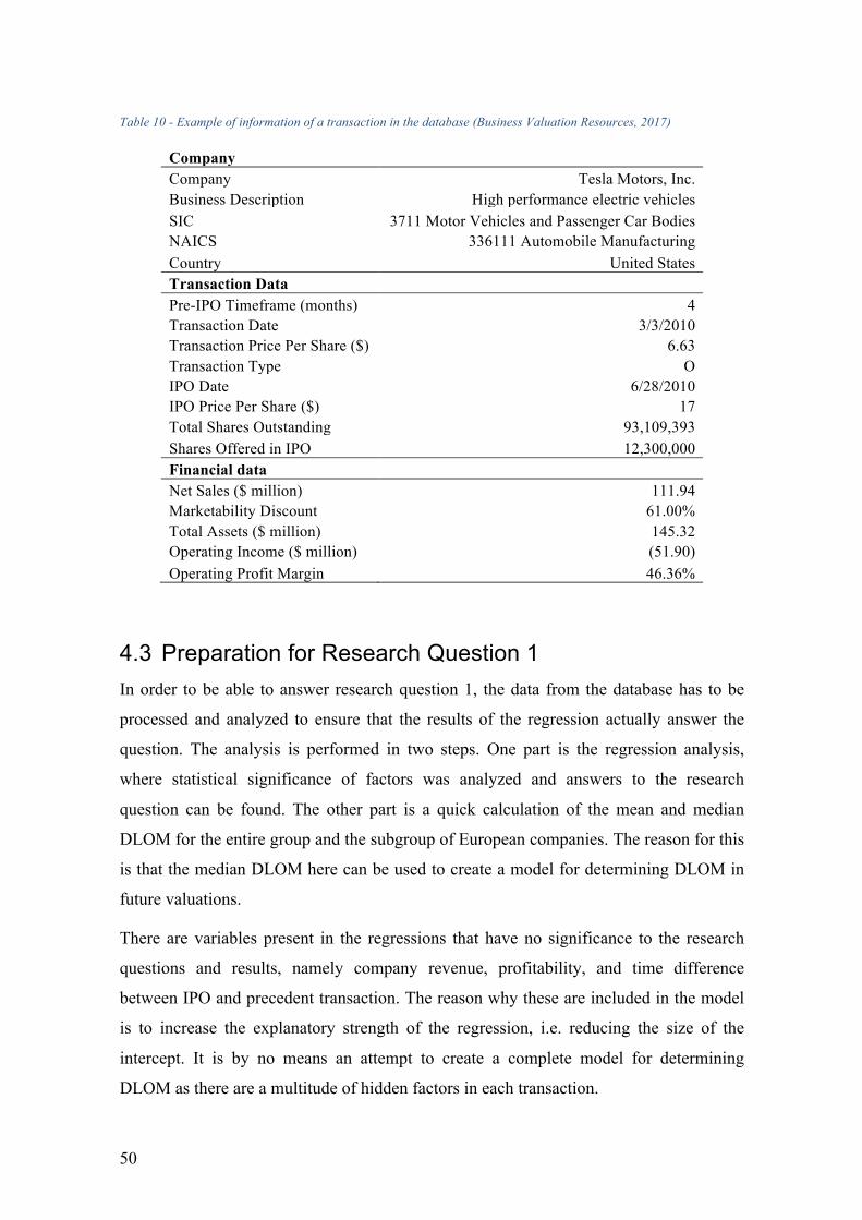
50

Table 10 - Example of information of a transaction in the database (Business Valuation Resources, 2017)

Company Company Tesla Motors, Inc.

Business Description High performance electric vehicles SIC 3711 Motor Vehicles and Passenger Car Bodies NAICS 336111 Automobile Manufacturing Country United States Transaction Data

Pre-IPO Timeframe (months) 4 Transaction Date 3/3/2010 Transaction Price Per Share ($) 6.63 Transaction Type O IPO Date 6/28/2010 IPO Price Per Share ($) 17 Total Shares Outstanding 93,109,393 Shares Offered in IPO 12,300,000 Financial data

Net Sales ($ million) 111.94 Marketability Discount 61.00% Total Assets ($ million) 145.32 Operating Income ($ million) (51.90) Operating Profit Margin 46.36%

4.3 Preparation for Research Question 1 In order to be able to answer research question 1, the data from the database has to be

processed and analyzed to ensure that the results of the regression actually answer the

question. The analysis is performed in two steps. One part is the regression analysis,

where statistical significance of factors was analyzed and answers to the research

question can be found. The other part is a quick calculation of the mean and median

DLOM for the entire group and the subgroup of European companies. The reason for this

is that the median DLOM here can be used to create a model for determining DLOM in

future valuations.

There are variables present in the regressions that have no significance to the research

questions and results, namely company revenue, profitability, and time difference

between IPO and precedent transaction. The reason why these are included in the model

is to increase the explanatory strength of the regression, i.e. reducing the size of the

intercept. It is by no means an attempt to create a complete model for determining

DLOM as there are a multitude of hidden factors in each transaction.

51

4.3.1 Data analysis Initially, the database contains information regarding more than 8,000 observations of

IPOs and precedent transactions over a time span of 30 years. This makes the Valuation

Advisors Lack of Marketability Discount database the largest of its kind in the world.

Furthermore, it is continuously updated with new transactions, which means that

reproduction of the data is impossible unless done shortly after the study. Completely

raw data can be found in the U.S. Securities Exchange Commission’s EDGAR database

or in internal documents of companies performing the IPO. Valuation Advisors records

the information found in these databases and gathers all necessary information that could

be used to derive a DLOM.

In the first research question, the goal is to identify differences in DLOM between

European and American companies. However, some European companies (mainly those

not members of EU or other trade unions) are omitted as they do not follow the same

financial regulations as the EU countries. Therefore, the countries that are present in the

study are:

• Austria • Belgium • Cyprus • Czech Republic • Denmark • France • Germany • Ireland • Italy • Luxembourg • Netherlands • Spain • Switzerland • United Kingdom

In addition, the countries omitted have few transactions and would likely become outliers

in the analysis. The chosen countries have a large variety of market properties, both in

terms of size and development. It can be argued that the number of companies in each

country is an indicator for the size of the country’s economy, meaning that the countries

implicitly are weighted according to size. Therefore, the countries together closely

represent the European economy.

52

Furthermore, information that is not necessary in the regression analysis is omitted. The

reason for the exclusion is that it is either not relevant for the study, or non-quantifiable

information. This information included:

• Company name • Transaction dates • SIC and NAICS codes • Operating profit • Revenue

Finally, observations where not all variables are present are omitted, as this could skew

the data.

4.3.2 European data analysis As seen above, there are large variations in the data, both in regards to average and

extreme values. The European dataset is much smaller than the U.S. equivalent, with 175

total transactions registered as compared to over 7,000. The spread of transactions over

the European countries can be seen in Table 11.

Table 11 - Number of transactions per European Country (own compilation)

Country Number Median DLOM Min Max Standard error Austria 3 29.76% 10.34% 89.07% 41.02% Belgium 2 5.67% 1.67% 9.67% 5.66% Cyprus 2 13.72% 13.72% 13.72% 0.00% Czech Republic 5 30.21% 30.21% 30.21% 0.00% Denmark 3 15.00% 0.95% 49.72% 25.10% France 22 45.28% 0.00% 86.18% 21.58% Germany 11 35.91% -32.00% 98.12% 37.37% Ireland 13 51.30% 1.74% 94.50% 29.74% Italy 3 48.11% -11.11% 60.44% 38.25% Luxembourg 4 -0.54% -32.00% 42.79% 35.45% Netherlands 37 47.10% -80.00% 93.08% 37.23% Spain 2 1.17% -65.00% 67.34% 93.58% Switzerland 10 8.22% 4.07% 20.33% 7.48% United Kingdom 58 55.03% -56.25% 96.97% 34.80% Total 175

As can be seen, the median DLOM is substantially higher in France than for instance

Czech Republic. This correlates with the fact that the French market is less volatile,

larger and more liquid than the Czech equivalent, however, no conclusions can be drawn

towards its causality. This is also not true for all pairs of countries, and in some cases, the

number of observations is so low that no patterns can be interpreted.

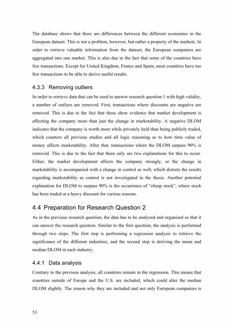
53

The database shows that there are differences between the different economies in the

European dataset. This is not a problem, however, but rather a property of the markets. In

order to retrieve valuable information from the dataset, the European companies are

aggregated into one market. This is also due to the fact that some of the countries have

few transactions. Except for United Kingdom, France and Spain, most countries have too

few transactions to be able to derive useful results.

4.3.3 Removing outliers In order to retrieve data that can be used to answer research question 1 with high validity,

a number of outliers are removed. First, transactions where discounts are negative are

removed. This is due to the fact that these show evidence that market development is

affecting the company more than just the change in marketability. A negative DLOM

indicates that the company is worth more while privately held than being publicly traded,

which counters all previous studies and all logic reasoning as to how time value of

money affects marketability. After that, transactions where the DLOM surpass 90% is

removed. This is due to the fact that there only are two explanations for this to occur.

Either, the market development affects the company strongly, or the change in

marketability is accompanied with a change in control as well, which distorts the results

regarding marketability as control is not investigated in the thesis. Another potential

explanation for DLOM to surpass 90% is the occurrence of “cheap stock”, where stock

has been traded at a heavy discount for various reasons.

4.4 Preparation for Research Question 2 As in the previous research question, the data has to be analyzed and organized so that it

can answer the research question. Similar to the first question, the analysis is performed

through two steps. The first step is performing a regression analysis to retrieve the

significance of the different industries, and the second step is deriving the mean and

median DLOM in each industry.

4.4.1 Data analysis Contrary to the previous analysis, all countries remain in the regression. This means that

countries outside of Europe and the U.S. are included, which could alter the median

DLOM slightly. The reason why they are included and not only European companies is

54

that there would be too few observations to return significance for every industry with

only European data. Since the purpose is to identify if and what industries that have

significantly higher or lower DLOM than average, the difference in mean DLOM does

not affect the thesis. In addition, it can be argued that most equity markets are global, and

thus foreign companies may be traded by the same investors as local companies.

The industries described in section 4.2 receive their own dummy variable. In addition to

these, the same independent variables as in first regression is used, and all other

information is omitted.

The industries with few data points are removed. In this case, the limit is set to less than

50, meaning that Agriculture, Construction, and Transportation/Public Utilities are

removed. The reason for this is that the low amount of data points means that the

significance of the test would be low. Usually, a rule of thumb is to have at least ten

observations per independent variable, but the fact that most factors are dummies means

that more observations are needed in order to return any significant information.

Therefore, the limit of number of observations is 50 in order to ensure that the data is

adequately large.

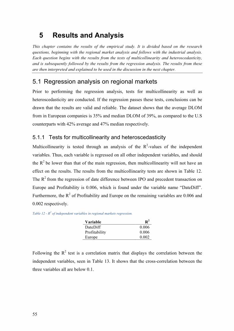
55

5 Results and Analysis This chapter contains the results of the empirical study. It is divided based on the research questions, beginning with the regional market analysis and follows with the industrial analysis. Each question begins with the results from the tests of multicollinearity and heteroscedasticity, and is subsequently followed by the results from the regression analysis. The results from these are then interpreted and explained to be used in the discussion in the next chapter.

5.1 Regression analysis on regional markets Prior to performing the regression analysis, tests for multicollinearity as well as

heteroscedasticity are conducted. If the regression passes these tests, conclusions can be

drawn that the results are valid and reliable. The dataset shows that the average DLOM

from in European companies is 35% and median DLOM of 39%, as compared to the U.S

counterparts with 42% average and 47% median respectively.

5.1.1 Tests for multicollinearity and heteroscedasticity Multicollinearity is tested through an analysis of the R2-values of the independent

variables. Thus, each variable is regressed on all other independent variables, and should

the R2 be lower than that of the main regression, then multicollinearity will not have an

effect on the results. The results from the multicollinearity tests are shown in Table 12.

The R2 from the regression of date difference between IPO and precedent transaction on

Europe and Profitability is 0.006, which is found under the variable name “DateDiff”.

Furthermore, the R2 of Profitability and Europe on the remaining variables are 0.006 and

0.002 respectively.

Table 12 - R2 of independent variables in regional markets regression.

Variable R2 DateDiff 0.006 Profitability 0.006 Europe 0.002

Following the R2 test is a correlation matrix that displays the correlation between the

independent variables, seen in Table 13. It shows that the cross-correlation between the

three variables all are below 0.1.

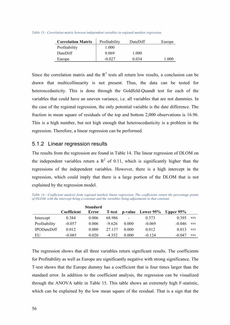
56

Table 13 - Correlation matrix between independent variables in regional markets regression.

Correlation Matrix Profitability DateDiff Europe Profitability 1.000

DateDiff 0.069 1.000 Europe -0.027 0.034 1.000

Since the correlation matrix and the R2 tests all return low results, a conclusion can be

drawn that multicollinearity is not present. Thus, the data can be tested for

heteroscedasticity. This is done through the Goldfeld-Quandt test for each of the

variables that could have an uneven variance, i.e. all variables that are not dummies. In

the case of the regional regression, the only potential variable is the date difference. The

fraction in mean square of residuals of the top and bottom 2,000 observations is 16.96.

This is a high number, but not high enough that heteroscedasticity is a problem in the

regression. Therefore, a linear regression can be performed.

5.1.2 Linear regression results The results from the regression are found in Table 14. The linear regression of DLOM on

the independent variables return a R2 of 0.11, which is significantly higher than the

regressions of the independent variables. However, there is a high intercept in the

regression, which could imply that there is a large portion of the DLOM that is not

explained by the regression model.

Table 14 - Coefficient analysis from regional markets linear regression. The coefficients return the percentage points of DLOM, with the intercept being a constant and the variables being adjustments to that constant.

Coefficient Standard

Error T-test p-value Lower 95% Upper 95%

Intercept 0.384 0.006 68.986 - 0.373 0.395 xxx

Profitability -0.057 0.006 -9.626 0.000 -0.069 -0.046 xxx

IPODateDiff 0.012 0.000 27.137 0.000 0.012 0.013 xxx

EU -0.085 0.020 -4.352 0.000 -0.124 -0.047 xxx

The regression shows that all three variables return significant results. The coefficients

for Profitability as well as Europe are significantly negative with strong significance. The

T-test shows that the Europe dummy has a coefficient that is four times larger than the

standard error. In addition to the coefficient analysis, the regression can be visualized

through the ANOVA table in Table 15. This table shows an extremely high F-statistic,

which can be explained by the low mean square of the residual. That is a sign that the

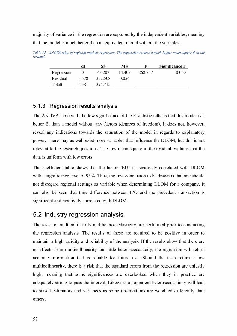
57

majority of variance in the regression are captured by the independent variables, meaning

that the model is much better than an equivalent model without the variables.

Table 15 - ANOVA table of regional markets regression. The regression returns a much higher mean square than the residual.

df SS MS F Significance F Regression 3 43.207 14.402 268.757 0.000 Residual 6,578 352.508 0.054

Totalt 6,581 395.715

5.1.3 Regression results analysis The ANOVA table with the low significance of the F-statistic tells us that this model is a

better fit than a model without any factors (degrees of freedom). It does not, however,

reveal any indications towards the saturation of the model in regards to explanatory

power. There may as well exist more variables that influence the DLOM, but this is not

relevant to the research questions. The low mean square in the residual explains that the

data is uniform with low errors.

The coefficient table shows that the factor “EU” is negatively correlated with DLOM

with a significance level of 95%. Thus, the first conclusion to be drawn is that one should

not disregard regional settings as variable when determining DLOM for a company. It

can also be seen that time difference between IPO and the precedent transaction is

significant and positively correlated with DLOM.

5.2 Industry regression analysis The tests for multicollinearity and heteroscedasticity are performed prior to conducting

the regression analysis. The results of these are required to be positive in order to

maintain a high validity and reliability of the analysis. If the results show that there are

no effects from multicollinearity and little heteroscedasticity, the regression will return

accurate information that is reliable for future use. Should the tests return a low

multicollinearity, there is a risk that the standard errors from the regression are unjustly

high, meaning that some significances are overlooked when they in practice are

adequately strong to pass the interval. Likewise, an apparent heteroscedasticity will lead

to biased estimators and variances as some observations are weighted differently than

others.

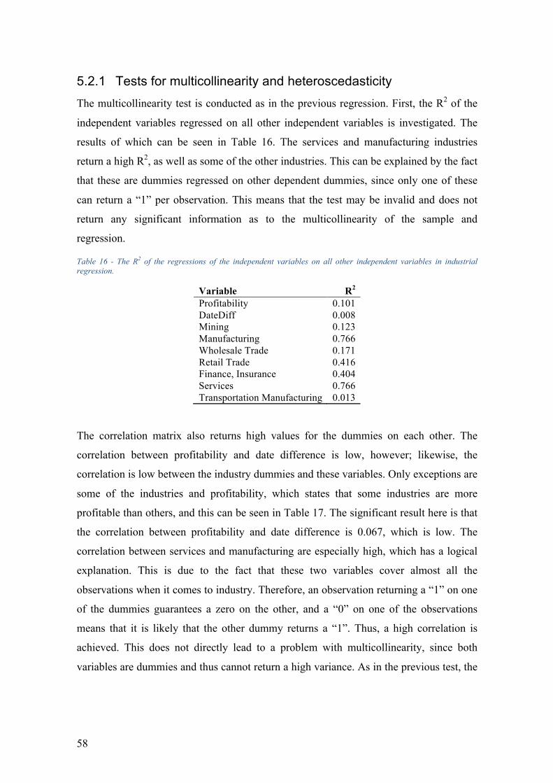
58

5.2.1 Tests for multicollinearity and heteroscedasticity The multicollinearity test is conducted as in the previous regression. First, the R2 of the

independent variables regressed on all other independent variables is investigated. The

results of which can be seen in Table 16. The services and manufacturing industries

return a high R2, as well as some of the other industries. This can be explained by the fact

that these are dummies regressed on other dependent dummies, since only one of these

can return a “1” per observation. This means that the test may be invalid and does not

return any significant information as to the multicollinearity of the sample and

regression.

Table 16 - The R2 of the regressions of the independent variables on all other independent variables in industrial regression.

Variable R2 Profitability 0.101 DateDiff 0.008 Mining 0.123 Manufacturing 0.766 Wholesale Trade 0.171 Retail Trade 0.416 Finance, Insurance 0.404 Services 0.766 Transportation Manufacturing 0.013

The correlation matrix also returns high values for the dummies on each other. The

correlation between profitability and date difference is low, however; likewise, the

correlation is low between the industry dummies and these variables. Only exceptions are

some of the industries and profitability, which states that some industries are more

profitable than others, and this can be seen in Table 17. The significant result here is that

the correlation between profitability and date difference is 0.067, which is low. The

correlation between services and manufacturing are especially high, which has a logical

explanation. This is due to the fact that these two variables cover almost all the

observations when it comes to industry. Therefore, an observation returning a “1” on one

of the dummies guarantees a zero on the other, and a “0” on one of the observations

means that it is likely that the other dummy returns a “1”. Thus, a high correlation is

achieved. This does not directly lead to a problem with multicollinearity, since both

variables are dummies and thus cannot return a high variance. As in the previous test, the

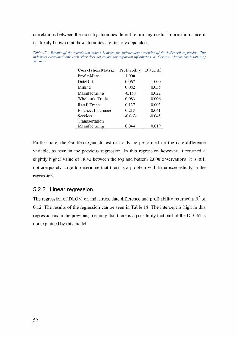
59

correlations between the industry dummies do not return any useful information since it

is already known that these dummies are linearly dependent.

Table 17 - Exempt of the correlation matrix between the independent variables of the industrial regression. The industries correlated with each other does not return any important information, as they are a linear combination of dummies.

Correlation Matrix Profitability DateDiff Profitability 1.000

DateDiff 0.067 1.000 Mining 0.082 0.035 Manufacturing -0.158 0.022 Wholesale Trade 0.083 -0.006 Retail Trade 0.137 0.003 Finance, Insurance 0.213 0.041 Services -0.063 -0.045 Transportation Manufacturing 0.044 0.019

Furthermore, the Goldfeldt-Quandt test can only be performed on the date difference

variable, as seen in the previous regression. In this regression however, it returned a

slightly higher value of 18.42 between the top and bottom 2,000 observations. It is still

not adequately large to determine that there is a problem with heteroscedasticity in the

regression.

5.2.2 Linear regression The regression of DLOM on industries, date difference and profitability returned a R2 of

0.12. The results of the regression can be seen in Table 18. The intercept is high in this

regression as in the previous, meaning that there is a possibility that part of the DLOM is

not explained by this model.

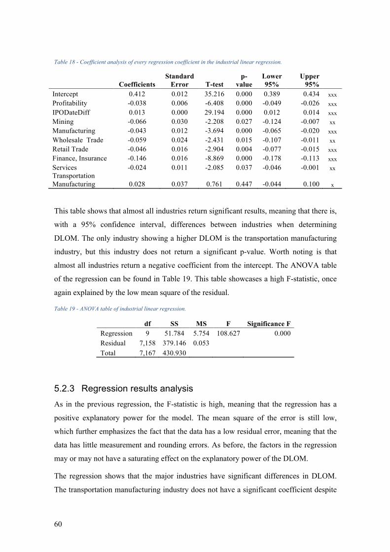
60

Table 18 - Coefficient analysis of every regression coefficient in the industrial linear regression.

Coefficients Standard

Error T-test p-

value Lower 95%

Upper 95%

Intercept 0.412 0.012 35.216 0.000 0.389 0.434 xxx Profitability -0.038 0.006 -6.408 0.000 -0.049 -0.026 xxx IPODateDiff 0.013 0.000 29.194 0.000 0.012 0.014 xxx Mining -0.066 0.030 -2.208 0.027 -0.124 -0.007 xx Manufacturing -0.043 0.012 -3.694 0.000 -0.065 -0.020 xxx Wholesale Trade -0.059 0.024 -2.431 0.015 -0.107 -0.011 xx Retail Trade -0.046 0.016 -2.904 0.004 -0.077 -0.015 xxx Finance, Insurance -0.146 0.016 -8.869 0.000 -0.178 -0.113 xxx Services -0.024 0.011 -2.085 0.037 -0.046 -0.001 xx Transportation Manufacturing 0.028 0.037 0.761 0.447 -0.044 0.100 x

This table shows that almost all industries return significant results, meaning that there is,

with a 95% confidence interval, differences between industries when determining

DLOM. The only industry showing a higher DLOM is the transportation manufacturing

industry, but this industry does not return a significant p-value. Worth noting is that

almost all industries return a negative coefficient from the intercept. The ANOVA table

of the regression can be found in Table 19. This table showcases a high F-statistic, once

again explained by the low mean square of the residual.

Table 19 - ANOVA table of industrial linear regression.

df SS MS F Significance F Regression 9 51.784 5.754 108.627 0.000 Residual 7,158 379.146 0.053

Total 7,167 430.930

5.2.3 Regression results analysis As in the previous regression, the F-statistic is high, meaning that the regression has a

positive explanatory power for the model. The mean square of the error is still low,

which further emphasizes the fact that the data has a low residual error, meaning that the

data has little measurement and rounding errors. As before, the factors in the regression

may or may not have a saturating effect on the explanatory power of the DLOM.

The regression shows that the major industries have significant differences in DLOM.

The transportation manufacturing industry does not have a significant coefficient despite

61

showing a clear difference in median DLOM. This regression also returns significant

values for time difference and profitability. The consistency of these results emphasize

the significance and importance of the factors in the determination of DLOM.

62

6 Discussion The discussion begins with an analysis of the three most commonly encountered research ethics. This is followed by a discussion on the data, method, results and subsequent analysis, where the results are compared to other metrics that could give indications to why some results have appeared and some not. Some comparisons to previous research and market characteristics are included for benchmarking purposes.

6.1 Research ethics Research ethics refers to the validity, reliability and generalizability of the thesis, and is a

way to measure how well the study holds in events of academic review.

6.1.1 Validity Validity, in this thesis, refers to the extent to which the test actually measures what it

intends to measure (Collis & Hussey, 2013). The test in this case intends to measure the

implied discount for lack of marketability and liquidity related to the company not being

publicly traded. Since the test uses actual market data, and is designed as to minimize the

time variance as factor for DLOM, it can be deemed to hold a high validity. However, the

independent variables used to increase the explanatory level of the regression are only a

few, and thus there may be other factors affecting the outcomes of the regression that are

overlooked.

Another remedy towards low validity is to avoid any selection bias when choosing what

companies to include in the study. There has already been a selection when the database

was created, as it does not include all countries, and only consists of companies that have

been adequately successful to be able to perform an IPO. In addition, only the successful

IPOs are represented and thus a large portion of potential companies are removed from

the study. However, one of the independent variables in the regression is whether or not a

company is profitable, and if this variable is shown to be insignificant, one can argue that

the “success” of a company is unrelated to the level of DLOM.

Considering how the results for the median DLOMs are similar to previous studies and

the fact that most of the other results are in line with the theory, the validity of the

empirical study can be seen as high. Through continuous recollection of the research

questions, the thesis has throughout the project been adapted so that the results definitely

return answers to the research questions, whether or not the results are positive.

63

6.1.2 Reliability Reliability refers to the accuracy of the study, and whether or not the results will change

if the study is to be repeated (Collis & Hussey, 2013). The factor that potentially could

vary if the study is to be repeated is the time. This is due to the fact that the regression is

performed on a large portion of the IPOs in the areas during a limited section of time, and

thus there is difficulties to find another sample on which the study could be reiterated.

Therefore, the level of reliability can be seen as high, and the only limiting factor is the

actual number of observations, since this affects the standard deviation of the results.

However, the database used is continuously updated. Once every month, new

transactions are added as more IPOs are performed worldwide. Therefore, replicating the

analysis with the exact same numbers is difficult and would require further limitations

regarding time series. This could also affect the results of future replications, since the

DLOM of the new transactions may differ from historic transactions. However, due to

the large number of transactions used, adding a few new would not significantly impact

the results; over a longer time period, the results may change.

In addition to the gathering of primary data, high reliability also requires accuracy and

strength of the secondary data. In order to ensure that high reliability is present in the

thesis, the secondary data search has been thorough and performed with an open mind. In

the instances of contradicting studies, all parties have been considered and their

reliability reviewed to objectively determine which is the most relevant and applicable to

the thesis. The use of course literature can sometimes be seen as having low reliability.

However, the literature used in this thesis is deemed to be very reliable as some have

hundreds of reviewers and others have thousands of citations. An example of course

literature that has been cited here is that of Copeland et al. (1991), which is seen to many

as the bible on corporate valuation. As it has been cited nearly 4,000 times according to

Google Scholar, it can safely be considered a reliable source. Another commonly cited

author is Shannon Pratt (2001, 2007 etc.), whom is one of the most reputable names

within corporate valuation. His books are more detailed and full of references than most

other literature on the subject, and are cited thousands of times according to Google

Scholar.

64

6.1.3 Generalizability Generalizability refers to the extent to which the results of a study can be applied

elsewhere. In this case, the generalizability of this study is rather low as it is specifically

designated to determine the level of DLOM, and nothing else. However, the

methodology that is used to find specific DLOM for some industries can also be applied

towards other industries in future research, which allows for some level of

generalizability. This exact methodology could be used to determine the other common

discounts added during a valuation. Using a database consisting of company takeovers,

where ownership pass the 50% mark, a regression would reveal the discount for lack of

control in the same way as the DLOM was derived from this database.

6.2 Discussion of data The data was of adequate size in order to determine some significant results, but not all.

Since it previously has been used to determine DLOM for certain populations, there was

no doubt that it could be used for our purpose as well.

6.2.1 Validity of the dataset The validity of the dataset can be questioned in several ways. First of all, the dataset is

compiled by hand by a number of analysts from multiple sources, creating a risk for

several selection and interpretation issues. Furthermore, the sources are of varying

quality. Even the SEC EDGAR database that most observations are derived from is not

completely perfect. It blindly relies on the reporting from the companies and the due

diligence process related to the IPO. In addition, it can be affected by the company

management not perfectly disclosing the transactions, but this is left for interpretation.

In addition, there is possibly a sample selection bias by the nature of the database. IPOs

are almost exclusively performed by successful companies and thus the value of the

companies can be expected to increase over the time of the IPO, as well as the time

between the precedent transaction and the IPO. This is clearly seen in the results from the

regressions, where the implied DLOM increases by 1.7% with every month separating

the precedent transaction from the IPO.

There is also an issue in the first research question regarding the regional segmentation,

due to the fact that only 2% of the transactions are European, whereas 90% are

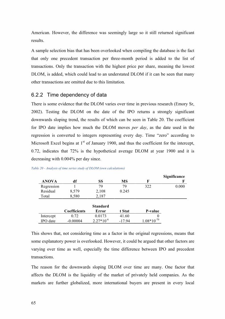
65

American. However, the difference was seemingly large so it still returned significant

results.

A sample selection bias that has been overlooked when compiling the database is the fact

that only one precedent transaction per three-month period is added to the list of

transactions. Only the transaction with the highest price per share, meaning the lowest

DLOM, is added, which could lead to an understated DLOM if it can be seen that many

other transactions are omitted due to this limitation.

6.2.2 Time dependency of data There is some evidence that the DLOM varies over time in previous research (Emory Sr,

2002). Testing the DLOM on the date of the IPO returns a strongly significant

downwards sloping trend, the results of which can be seen in Table 20. The coefficient

for IPO date implies how much the DLOM moves per day, as the date used in the

regression is converted to integers representing every day. Time “zero” according to

Microsoft Excel begins at 1st of January 1900, and thus the coefficient for the intercept,

0.72, indicates that 72% is the hypothetical average DLOM at year 1900 and it is

decreasing with 0.004% per day since.

Table 20 - Analysis of time series study of DLOM (own calculations)

ANOVA df SS MS F Significance

F Regression 1 79 79 322 0.000 Residual 8,579 2,108 0.245

Total 8,580 2,187

Coefficients

Standard Error t Stat P-value

Intercept 0.72 0.0173 41.60 0 IPO date -0.00004 2.27*10-6 -17.94 1.08*10-70

This shows that, not considering time as a factor in the original regressions, means that

some explanatory power is overlooked. However, it could be argued that other factors are

varying over time as well, especially the time difference between IPO and precedent

transactions.

The reason for the downwards sloping DLOM over time are many. One factor that

affects the DLOM is the liquidity of the market of privately held companies. As the

markets are further globalized, more international buyers are present in every local

66

market. This means that there are more potential buyers for every privately held

company. While this could affect the company prices since the competition is stronger, it

mitigates the lack of marketability in the markets.

6.3 Discussion of Method The quantitative method has previously been accredited for determining DLOM through

the numerous previous pre-IPO studies. The method will thus be discussed further below,

but with emphasis on the technical details such as the confidence interval,

multicollinearity and heteroscedasticity.

6.3.1 Confidence interval Representing two standard deviations, the 95% confidence interval of the regression

outputs is often considered the standard for presentation of regression results. Since it

means that 95% of all outcomes should land within the range, it is a fairly safe

measurement for the results, excluding outliers and measurement errors. It is worth

noting that this analysis by no means return absolute results. The only conclusion that

safely could be drawn is that, for a factor with a p-value below 0.05, one can discard the

hypothesis that there is no difference related to the factor, with 95% confidence. Several

factors with such p-values have been retrieved from the regression analysis.

6.3.2 Regression methodology The removal of outliers and specific data points could have an impact on the reliability of

the study. In a way, there is a trade-off between validity and reliability since the removal

of outliers means that the possibility to answer the research questions increases, but at the

cost of reliability since there may be a selection bias while removing observations.

The multicollinearity and heteroscedasticity tests are essential to maintain a high validity

in the study. However, the Goldfeld-Quandt test is difficult to apply when several of the

variables are dummies as there cannot be any difference in variance between the top and

bottom parts of the samples. Therefore, it could only be performed on the other variables,

with an assumption that there is no risk for heteroscedasticity in dummy variables.

Performing another regression method could have an impact on the results. For instance,

a t-test sometimes return completely different results than a confidence test and

multivariate linear regression. In this case, the dataset could not be assumed to be

67

normally distributed, thus a F-statistic is preferred over a t-test. However, partially due to

the fact that the linear regression and confidence tests are accredited methods, and

partially due to the fact that previous empirical studies of DLOM has used these models,

the most logical models to use are the linear regression with ANOVA presentation and

confidence tests. Therefore, the academic validity of previous studies (see chapter three)

is adequate proof to the use of this quantitative model for determining DLOM.

6.4 Discussion of Results Due to the large amount of observations, most results display significant differences,

even if they are small. This is positive as it allows for accurate determination of DLOM

for future valuations as it can not vary substantially within a certain significance level.

6.4.1 Significance of regression results The results return several significant factors, some of which with strong significance.

Some of the results are correlated with previous studies, while others have indications of

opposite trends. The fact that some results have opposite trends compared with theory

shows that there might be a risk that the other, significant results are wrong. However,

the conclusion can also be drawn that the results show true information for the specific

data set, meaning that it is true for the set of companies that are included in the database.

Despite having more than 8,000 data points, some results show low significance. This is

an indication that the data has a high variance and probably has many outliers. Therefore,

one can question the validity of the results from some of the regressions, especially

regarding some industries with few transactions. The only conclusions that can be drawn

is that, for this dataset, there are factors that are significant with 95% confidence.

However, it does not mean that the factors are significant for another, similar dataset.

The R2 statistic of the regression is an indication of the explanatory power of the model.

For all regressions in this thesis, the R2 is low (just above 0.1), thus the explanatory

power is low. However, the intention is never to achieve a high explanatory power, only

give indications as to what could be worth investigating from an analyst’s point of view.

Especially since the most important factor for DLOM is excluded, namely marketability,

a low explanatory power is expected.

68

6.4.2 Results of profitability and date difference It is apparent that both profitability and date difference between IPO and precedent

transactions are significant for determining DLOM. The question remains how to

interpret the strong correlation between DLOM and date difference and profitability.

There is a negative correlation between profitability and DLOM, which means that

profitable companies are either worth more while privately held, or worth less while

public. Furthermore, the strong positive correlation between date difference and DLOM

indicates that time is a factor that has to be considered when determining DLOM, but this

could be interpreted in other ways. Assuming an IPO takes around six months to

perform, then a company normally never has more marketability inhibition than a six-

month time span. With this logic, one could argue that six times the average monthly

discount increase should be added for a company that has yet to start its IPO process or

any private transaction.

6.4.3 Results in relation to control discount/premiums The issue that has not been covered here is whether or not the level of control has similar

factors and drivers as marketability. Since the two adjustments often are used in

conjunction, this would be relevant for determining the total adjustment. Some analysts

argue that normally for privately held majority shares, the level of DLOM cancels out the

premium added for control. Our findings determine that this is a broad assumption that

may lead to a skewed valuation. Especially in industries that have a median DLOM far

from the total sample, the DLOM and control premium may differ with more than 20

percentage points.

This study has taken no consideration regarding adjustments for changes in control. This

is due to the fact that the database only regards IPOs where the level of control does not

change between transactions. A similar study with the exact same methodology could be

performed for a database with private transactions, where the level of control changes.

6.4.4 Results in relation to previous studies Since the study used a database that previously has been used and accredited for

determining DLOM, the results for average DLOM overlaps previous studies. However,

these studies do not consider the industry factor, nor present differences between Europe

and the U.S.

69

The study in this thesis has a larger spread of companies than the Emory studies, which

removed companies that were in a development stage, had operating losses, less than $5

per share IPO price and companies that were not American. Likewise, the WMA studies

excluded transactions involving compensation-related stock as well as transactions

involving corporate insiders. The fact that our study included all of these companies

means that there is a risk for more outliers and skewed results, but the sample used

represents the markets better than the Emory studies.

Valuation Advisors LLC., the founders of the database used in the study, retrieved a 41%

to 54% one-year DLOM after removing outliers below 10% and above 90%. This is close

to our findings that DLOM range between 28% and 40% for a 0-year DLOM, with

another 1.2% added per month. Valuation Advisors also found that, the closer to an IPO

a company is, the more marketable it becomes, and less discount should be applied.

Option pricing models all incorporate time to marketability as a factor for the discount,

which makes them comparable to the study in this thesis. However, all of these studies

display a higher variance based on time than the pre-IPO studies. This could be explained

by the large differences in the volatility used in the option studies; the volatility is a

required variable for option pricing according to the Black-Scholes model. These models

also have broad assumptions regarding the volatility of privately held stock, which could

affect the results. Another issue with option pricing models is that there is no way to

incorporate other factors than those present in the Black-Scholes model. Instead, proxies

have to be used for the variables, where the volatility in the model represents industries,

the discount rate representing risk, among other factors.

6.5 Discussion of analysis Conclusions can only be drawn regarding significant results from the regressions, for a

predetermined level of significance. Everything else can be seen as indications, but does

not hold any academic validity and cannot be used for future references.

6.5.1 Discussion on the differences between Europe and USA There are several factors that differ between the markets in the U.S. and Europe. One

factor that theoretically would cause higher DLOM on the European markets is the added

risk for currency exchange rates. The U.S. dollar is the most traded currency in the world,

and several other globally used currencies are pegged towards it, among those the

70

Chinese Yuan as well as most currencies in the Middle East. Therefore, the Euro, as well

as the currencies used in the smaller stock exchanges in Europe, is naturally more volatile

than the US dollar. Since volatility is positively correlated to duration of non-

marketability, higher volatility leads to higher marketability discount.

However, another important difference appears as well. The European public markets are

less liquid than the U.S. counterparts. While this makes no difference to privately held

companies, the result is that there is a shorter liquidity gap between private and public

companies in Europe as compared to the U.S. This implies that, while conclusions cannot

be drawn as to the liquidity of either public or private markets in Europe and the U.S., the

difference between the liquidity of private and public markets is smaller in Europe than

the U.S. Thus, the discount based on liquidity should naturally be less in Europe than in

the U.S. As it seems, the effects due to liquidity is less prominent than those due to

currency risk, causing a lower DLOM in European markets.

One large difference between markets of privately held companies in Europe and U.S. is

the difference in capital acquisition processes. European companies rely on bank lending

to a much greater extent, with 80% of capital is formed through corporate debt and 20%

from corporate bonds. The opposite is found in the U.S. private equity market (CME

Group, 2015).

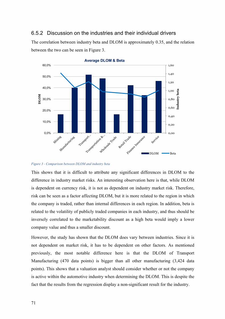
71

6.5.2 Discussion on the industries and their individual drivers The correlation between industry beta and DLOM is approximately 0.35, and the relation

between the two can be seen in Figure 3.

Figure 3 - Comparison between DLOM and industry beta

This shows that it is difficult to attribute any significant differences in DLOM to the

difference in industry market risks. An interesting observation here is that, while DLOM

is dependent on currency risk, it is not as dependent on industry market risk. Therefore,

risk can be seen as a factor affecting DLOM, but it is more related to the region in which

the company is traded, rather than internal differences in each region. In addition, beta is

related to the volatility of publicly traded companies in each industry, and thus should be

inversely correlated to the marketability discount as a high beta would imply a lower

company value and thus a smaller discount.

However, the study has shown that the DLOM does vary between industries. Since it is

not dependent on market risk, it has to be dependent on other factors. As mentioned

previously, the most notable difference here is that the DLOM of Transport

Manufacturing (470 data points) is bigger than all other manufacturing (3,424 data

points). This shows that a valuation analyst should consider whether or not the company

is active within the automotive industry when determining the DLOM. This is despite the

fact that the results from the regression display a non-significant result for the industry.

0,00

0,20

0,40

0,60

0,80

1,00

1,20

1,40

1,60

0,0%

10,0%

20,0%

30,0%

40,0%

50,0%

60,0%

Indu

stry

bet

a

DLO

M

Average DLOM & Beta

DLOM Beta

72

The Service industry has a higher marketability discount than most other industries. This

could be explained by several factors. One factor that could lead to a higher discount is

the fact that service companies often are more human resource based than for instance

industry companies, and thus have less tangible assets. This means that the service

companies are valued lower to some investors that value net assets rather than future cash

flows. At the same time, service companies often contain stronger synergies with other

companies as compared to, for instance, mining. Thus, private equity investors should be

more interested in buying service companies for their portfolios. Therefore, from an

M&A point of view, the DLOM should be smaller for service companies. It can also be

seen that the larger industries (in number of transactions) have a higher DLOM, with for

instance services median 50% and mining 37%.

6.6 Sustainability The results of this thesis does not have any implications as to either environmental or

social sustainability. The third pillar of sustainability, namely Economic sustainability, is

the ability of an economy to support a defined level of economic production indefinitely.

While this thesis does not assist in any means of production, it does imply that there are

some industries in which companies are worth more relatively while privately held. This

means that there is a larger profit, for the same means of production, in some industries

rather than others, and this thesis intends to assist valuation professionals to ensure that

the owners of these companies are paid their fair share for their work. The results of this

is a fairer distribution of capital, and more accurate valuations of incentive programs of

employees of privately held companies.

73

7 Conclusion This chapter summarizes the results and discussion into a conclusion. It begins with an explanation of the key findings from the study, which ends with a suggestion for a model for determining DLOM in future valuations. This is followed by implications for valuation analysts and subsequently suggestions for future research.

7.1 Key findings To recollect, the first research question was formulated as follows:

How much does the marketability discount differ in value between European registered

companies and US equivalents?

The answer to the first research question is that consideration should be taken regarding

the region in which the company is located. The results show that there is an 8.0% lower

DLOM for European companies than the U.S. counterparts with a 2% standard deviation,

and this should be reflected in the valuation of privately held companies in the areas.

This result implies that the difference in value between privately held and publicly traded

companies are smaller in Europe than in the U.S. leading to a lower DLOM in Europe.

This could be explained by the fact that the U.S. public market is more liquid than the

European, thus leading to a higher difference in liquidity from privately held companies.

The regression also displayed that the profitability of the company is an important factor

for determining DLOM, with a 5.7% lower discount for profitable companies as

compared to non-profitable with a 0.6% standard deviation. The differences between the

U.S. and Europe are discussed based on the higher liquidity in the public traded sector,

lower transaction costs and currency effects. The European market is more volatile, less

homogeneous and more characterized by bank lending, while the U.S. market is

characterized by corporate bond issuing and a more mature venture capital market with

more transparency.

The second research question was formulated as follows:

To what extent, and what are the explanatory factors to the marketability discount


The second regression analysis answers the second research question and show that the

investigated industries differ in the amount of DLOM applied on each industry. Further it

implies that e.g. the finance/insurance industry should carry an approximately 12% lower

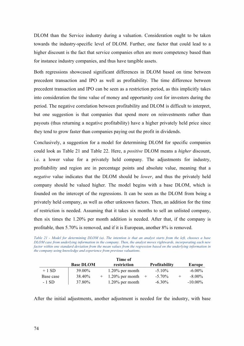
74

DLOM than the Service industry during a valuation. Consideration ought to be taken

towards the industry-specific level of DLOM. Further, one factor that could lead to a

higher discount is the fact that service companies often are more competency based than

for instance industry companies, and thus have tangible assets.

Both regressions showcased significant differences in DLOM based on time between

precedent transaction and IPO as well as profitability. The time difference between

precedent transaction and IPO can be seen as a restriction period, as this implicitly takes

into consideration the time value of money and opportunity cost for investors during the

period. The negative correlation between profitability and DLOM is difficult to interpret,

but one suggestion is that companies that spend more on reinvestments rather than

payouts (thus returning a negative profitability) have a higher privately held price since

they tend to grow faster than companies paying out the profit in dividends.

Conclusively, a suggestion for a model for determining DLOM for specific companies

could look as Table 21 and Table 22. Here, a positive DLOM means a higher discount,

i.e. a lower value for a privately held company. The adjustments for industry,

profitability and region are in percentage points and absolute value, meaning that a

negative value indicates that the DLOM should be lower, and thus the privately held

company should be valued higher. The model begins with a base DLOM, which is

founded on the intercept of the regressions. It can be seen as the DLOM from being a

privately held company, as well as other unknown factors. Then, an addition for the time

of restriction is needed. Assuming that it takes six months to sell an unlisted company,

then six times the 1.20% per month addition is needed. After that, if the company is

profitable, then 5.70% is removed, and if it is European, another 8% is removed.

Table 21 - Model for determining DLOM (a). The intention is that an analyst starts from the left, chooses a base DLOM case from underlying information in the company. Then, the analyst moves rightwards, incorporating each new factor within one standard deviation from the mean values from the regression based on the underlying information in the company using knowledge and experience from previous valuations.

Base DLOM

Time of restriction

Profitability

Europe

+ 1 SD 39.00%

1.20% per month

-5.10%

-6.00% Base case 38.40% + 1.20% per month + -5.70% + -8.00% - 1 SD 37.80%

1.20% per month

-6.30%

-10.00%

After the initial adjustments, another adjustment is needed for the industry, with base

75

numbers in the middle in conjunction with a standard deviation of variation in each

direction.

Table 22 - Model for determining DLOM (b)

Mining Manufacturing Wholesale Trade Retail Trade Finance/insurance Services -3.60% -3.10% -3.50% -3.00% -13.00% -1.30% -6.60% -4.30% -5.90% -4.60% -14.60% -2.40% -9.60% -5.50% -8.30% -6.20% -16.20% -3.50%

The standard deviations are included as the model does not fully explain the DLOM. Soft

factors, such as ownership, management and key persons could affect the DLOM as well,

and thus the standard deviations are included to allow for the valuation analyst to draw

conclusions in both directions.

7.2 Implications and contributions This master thesis intends to contribute to both academia as well as the professional

standards of valuation experts with an increased understanding and accuracy of the

application of DLOM.

7.2.1 Contributions to academic literature The academic contribution from this thesis is the focus of DLOM for European

companies and a review of how the discount differs between markets. While the area of

marketability discounts is well developed, mainly by Pratt (2001; 2008) and Novak

(2016), little regards have been taken towards differences between markets. The results

can thus be supportive in the development of future valuation models.

7.2.2 Implications for valuation analysts The research indicates two things for valuation analysts. Firstly, consideration should be

taken towards industry and region differences between companies. Using a global

average of all companies does not represent most companies in the value of the DLOM.

Secondly, the large variance of DLOM means that it is a potentially large error to assume

that the marketability discount cancels out the control premium for privately held

majority shares. Since the marketability discount varies with more than 20%, this has to

be taken into consideration to fully reflect the market value of a company in a valuation.

76

7.3 Future Research This research could be further tested by using a different source of data. The large

variance in the database shows that it could have a large effect on the results.

In addition, this research should be coupled with a similar study on control discounts and

premiums, where the control adjustment is tested for specific industries and regions.

Only then can conclusions be drawn as to whether or not the control premium cancels

marketability discounts for privately held majority shares.

This model for marketability is by no means complete, as seen in the high intercepts of

the regressions. A study could be performed to try to increase the explanatory power of

the model, for instance by including information regarding the buy-side and sell-side of

the transactions. Removing outliers due to cheap stock or stock market changes would

also increase the accuracy of the model.

The model could be extended with both hard and soft factors. An important factor that

could be considered is the management, which is difficult to quantify. Using a qualitative

study to capture psychological factors and incorporate behavioral finance would likely

return other significant factors for determining DLOM.

In addition, doing similar regressions for the Mandelbaum factors would be a great

supplement in a legal context. This would however require much more analysis regarding

every transaction, and thus an 8,000 company sample would take a long time. Applying

the Mandelbaum factors on a European dataset would add value for European court cases

to determine DLOM in future valuation disputes.

77

Bibliography AICPA. (2011). International Glossary of Business Valuation Terms. Aktiebolagslag. (2005:551). Justitiedepartementet L1. Bachelier, L. (1900). Théorie de la spéculation. Gauthier-Villars. Bajaj et al. (2001). Firm Value and Marketability Discounts. Journal of Corporation Law . Berk, J. B., & DeMarzo, P. M. (2014). Corporate Finance. Pearson Education. Bernström, S. (2014). Valuation: The Market Approach. Chichester: John Wiley & Sons. Black, F., & Scholes, M. (1973). The pricing of options and corporate liabilities. Journal of Political Economy , 637-654. Business Valuation Resources. (2017). Deal & Market Data. Retrieved 05 01, 2017, from Business Valuation Resources: https://www.bvresources.com/products/deal-and-market-data Canadas, J. A., & Rojo Ramirez, A. A. (2011). The discount rate in valuing privately held companies. Chaffee III, D. B. (1993). Option pricing as a proxy for discount for lack of marketability in private company valuations. Business Valuation Review , 182-188. CME Group. (2015, 10 29). Open Markets. Retrieved 05 26, 2017, from How U.S. and EU capital markets are different.: http://openmarkets.cmegroup.com/10431/how-u-s-and-eu-capital-markets-are-different Collis, J., & Hussey, R. (2013). Business research: A practical guide for undergraduate and postgraduate students. London: Palgrave Macmillan. Damodaran, A. (2005). The value of control: Implications for control premia, minority discounts and voting share differentials. New York: Stern School of Business. Damodaran, A. (2017, 01). Total Beta per Industry. Retrieved 05 03, 2017, from http://pages.stern.nyu.edu/~adamodar/New_Home_Page/datafile/totalbeta.html Elmore, J. E. (2017). Determining the Discount for Lack of Marketability with Put Option Pricing Models in View of the Section 2704 Proposed Regulations. Insights , 32-93. Emory Sr, J. D. (2002). Discounts for lack of marketability: Emory Pre-IPO discount studies 1980-2000, as adjusted October 10, 2002. Business Valuation Review , 190-191. Estate of Mitchell v. Commissioner, 872 (Tax Court Memo 1997). Fama, E. F. (1991). Efficient capital markets II. The Journal of Finance , 1575-1617. Fama, E. F. (1970). Efficient capital markets: A review of theory and empirical work. The Journal of Finance , 383-417. Finnerty, J. D. (2013). Using put option-based DLOM models to estimate discounts for lack of marketability. Business Valuation Review , 165-170. Garland, P., & Reilly, A. (2004). Update on the Willamette Management Associates Pre-IPO Discount for Lack of Marketability Study for the Period 1998 Through 2002. Insights (Williamette Management Associates) .

78

Gordon, E. L. (1952). What is fair market value. Tax L. Rev. , 35. Hall, L. S. (2009). The use of theoretical models to estimate the discount for lack of marketability. Gift and Estate Tax Valuation Insights , 7-12. Hertzel, M., & Smith, R. L. (1993). Market discounts and shareholder gains for placing equity privately. The Journal of Finance , 459-485. Internal Revenue Service. (2009). Discount for Lack of Marketability: Job Aid for IRS Valuation Professionals. IRS. Jennergren, L. P. (1998). A tutorial on the discounted cash flow model for vlauation of companies. SSE/EFI Working Paper Series in Business Administration . Jensen, M. C. (1978). Some anomalous evidence regarding market efficiency. Journal of Financial Economics , 95-101. Kennedy, P. (2011). A Guide to Econometrics. Oxford: Wiley-Blackwell. Koller et al. (2015). Valuation: measuring and managing the value of companies (Sixth Edition ed.). New York: Wiley. Lance, T. R. (2009). The use of theoretical models to estimate the discount for lack of marketability. BVR's Guide to Discounts for Lack of Marketability . Laro, D., & Pratt, S. P. (2005). Business valuation and taxes: Procedure, law, and perspective. New Jersey: John Wiley & Sons. Ljungqvist, A., & Wilhelm, W. (2005). Does prospect theory explain IPO market behavior? The Journal of Finance , 1759-1790. Loewenstein, G., & Thaler, R. H. (1989). Anomalies: intertemporal choice. The Journal of Economic Perspectives , 181-193. Longstaff, F. A. (1995). How much can marketability affect security values? The Journal of Finance , 1767-1774. Mandelbaum v. Commissioner, 255 (Tax Court Memo 1995). Mercer, Z. C. (2001). Quantifying Marketability Discounts: Developing and supporting marketability discounts in the appraisal of closely held business interests. Peabody. Mercer, Z. C., & Harms, T. W. (2015). The Quantitative Marketability Discount Model: A shareholder level DCF model. Business Valuation Discounts and Premiums , 2, 213-224. Merton, R. C. (1976). Option pricing when underlying stock returns are discontinuous. Journal of Financial Economics , 125-144. Miclea, C. S., & Sacui, V. (2012). The levels of value in business valuation: The Discount for Lack of Marketability. Anale. Seria Stiinte Economice , 572. Modigliani, F., & Miller, M. H. (1958). The cost of capital, corporate finance and the theory of investment. The American Economic Review , 261-297. Montgomery et al. (2015). Introduction to linear regression analysis. New Jersey: John Wiley & Sons. Moroney, R. E. (1973). Most courts overvalue closely held stocks. Taxes , 144. Nilsson et al. (2002). Företagsvärdering med fundamental analys. Studentlitteratur.

79

Novak, N. P. (2016). Measuring the Discount for Lack of Marketability for Noncontrolling, Nonmarketable Ownership Interests. Gift and Estate Tax Valuation Insights . Novak, N. P. (2014). Regression Analysis and the Discount for Lack of Marketability . Insights , 86-92. Pearl, J., & Rosenbaum, J. (2013). Investment banking: valuation, leveraged buyouts, and mergers and acquisitions. New Jersey: John Wiley & Sons. Pindyck, R. S., & Rubinfeld, D. L. (1998). Econometric Models and Economic Forecasts. Singapore: Irwin/McGraw-Hill. Pratt, S. P. (2009). Business Valuation: Discounts and premiums. John Wiley & Sons. Pratt, S. P. (2001). Discounts and Premiums. New York. Pratt, S. P., & Niculita, A. V. (2000). The lawyer's business valuation handbook. Chicago: American Bar Association. Pratt, S. P., & Niculita, A. V. (2008). Valuing a Business: The Analysis and Appraisal of Closely Held Companies. McGraw-Hill. PwC. (2011). Roadmap for an IPO: A guide to going public. PwC. Reilly, R., & Rotkowski, A. (2007). The discount for lack of marketability: update on current studies and analysis of current controversies. The Tax Lawyer , 241-286. Ritter, J. R., & Welch, I. (2002, 08). A Review of IPO Activity, Pricing and Allocations. The Journal of Finance , 1795-1828. Rozeff, M. S., & Kinney, W. R. (1976). Capital market seasonality: The case of stock returns. Journal of Financial Economics , 379-402. Saunders, P. (2000). Marketability discounts and risks in transactions prior to IPOs. Business Valuation Review , 186-195. Sharpe, W. F. (1964). Capital asset prices: A theory of market equillibrium under conditions of risk. The Journal of Finance , 425-442. Silber, W. L. (1991). Discounts on restricted stock: The impact of illiquidity on stock prices. Financial Analysts Journal , 60-64. Subrahmanyam, A., & Titman, S. (1999). The Going-Public Decision and the Development of Financial Markets. The Journal of Finance , 1045-1082. TEGoVA. (2016). European Valuation Standards. Trout, R. R. (1977). Estimation of the discount associated with the transfer of restricted securities. Taxes , 381-384. U.S. S.E.C. (2015, 01 25). CF SIC code list. Retrieved 05 12, 2017, from U.S. Securities and Exchance Commission: https://www.sec.gov/info/edgar/siccodes.htm

www.kth.se

Discounts for Lack of Marketability...Abstract Discount for Lack of Marketability (DLOM) is one of...

Documents

Transcript of Discounts for Lack of Marketability...Abstract Discount for Lack of Marketability (DLOM) is one of...