DISCLAIMER - ARM Climate Research Facility AMF Doppler Lidar . ARM Atmospheric Radiation Measurement...

DISCLAIMER

This report was prepared as an account of work sponsored by the U.S. Government. Neither the United States nor any agency thereof, nor any of their employees, makes any warranty, express or implied, or assumes any legal liability or responsibility for the accuracy, completeness, or usefulness of any information, apparatus, product, or process disclosed, or represents that its use would not infringe privately owned rights. Reference herein to any specific commercial product, process, or service by trade name, trademark, manufacturer, or otherwise, does not necessarily constitute or imply its endorsement, recommendation, or favoring by the U.S. Government or any agency thereof. The views and opinions of authors expressed herein do not necessarily state or reflect those of the U.S. Government or any agency thereof.

DOE/SC-ARM-TR-101

Doppler Lidar (DL) Handbook RK Newsom February 2012 Work supported by the U.S. Department of Energy, Office of Science, Office of Biological and Environmental Research

RK Newsom, February 2012, DOE/SC-ARM-TR-101

iii

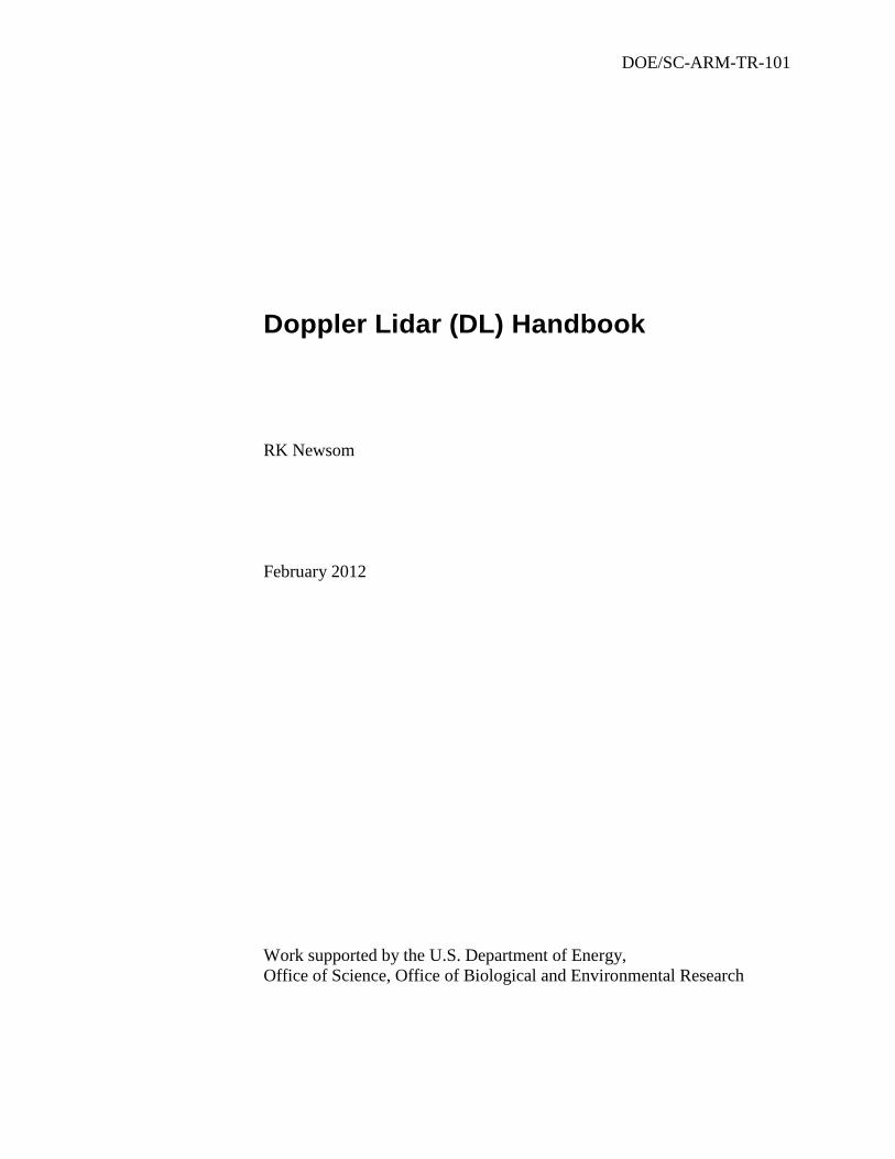
Acronyms and Abbreviations

AGL above ground level AMF ARM Mobile Facility AMFDL AMF Doppler Lidar ARM Atmospheric Radiation Measurement DL Doppler Lidar DMF Data Management Facility DOE U.S. Department of Energy DQO Data Quality Office GVAX Ganges Valley Aerosol Experiment LIDAR Light Detection and Ranging LO Local Oscillator LLJ low-level jet PNNL Pacific Northwest National Laboratory PPI Plan-Position-Indicator QME Quality Measurement Experiment RF radio frequency RHI range-height-indicator SDS site data system SGP Southern Great Plains SGPDL Southern Great Plains Doppler Lidar SNR signal-to-noise ratio TWP Tropical Western Pacific TWPDL Tropical Western Pacific Doppler Lidar VAD velocity-azimuth display VAP value-added product

Also see the ARM Acronyms and Abbreviations.

http://www.arm.gov/about/acronyms


iv

Contents

1.0 General Overview ................................................................................................................................. 1 2.0 Contacts ................................................................................................................................................ 1

2.1 Mentor .......................................................................................................................................... 1 2.2 Vendor / Instrument Developer .................................................................................................... 2

3.0 Deployment Locations and History ...................................................................................................... 2 4.0 Near-Real-Time Data Plots .................................................................................................................. 3 5.0 Data Description and Examples ........................................................................................................... 4

5.1 Data File Contents ........................................................................................................................ 4 5.2 Annotated Examples .................................................................................................................... 5

6.0 Data Quality .......................................................................................................................................... 7 6.1 Measurement Uncertainty ............................................................................................................ 7 6.2 Data Quality Health and Status .................................................................................................. 10 6.3 Data Reviews by Instrument Mentor.......................................................................................... 10 6.4 Data Assessments by Site Scientist/Data Quality Office ........................................................... 10

7.0 Value-Added Products ........................................................................................................................ 10 8.0 Instrument Details............................................................................................................................... 10

8.1 Detailed Description ................................................................................................................... 10 8.1.1 List of Components ......................................................................................................... 10 8.1.2 System Configuration and Measurement Methods ......................................................... 11 8.1.3 Specifications .................................................................................................................. 12

8.2 Theory of Operation ................................................................................................................... 12 8.3 Calibration .................................................................................................................................. 14 8.4 Operation and Maintenance ....................................................................................................... 15

8.4.1 User Manual .................................................................................................................... 15 8.4.2 Routine and Corrective Maintenance Documentation .................................................... 15

8.5 Glossary ...................................................................................................................................... 15 8.6 Citable References...................................................................................................................... 15


v

Figures

1 Deployment locations of the ARM Doppler lidars circa November 2011. ........................................... 2 2 Height-time displays of vertical staring data from the SGPDL and the TWPDL. ............................... 6 3 Radial velocity and attenuated backscatter data from an RHI scan acquired by the AMFDL

during GVAX at ~1717 UTC on 3 October 2011. ................................................................................ 6 4 Time-height display of the mean horizontal winds derived from SGPDL data for the period

from 26 through 28 September 2011. ................................................................................................... 7 5 Radial velocity and backscatter intensity during side-by-side intercomparisons of the

TWPDL and SGPDL from 2200 to 2300 UTC on 18 October 2010. ................................................... 8 6 The top panel shows the difference in radial velocity between the TWPDL and SGPDL from

2200 to 2300 UTC on 18 October 2010 ................................................................................................ 8 7 Estimates of radial velocity precision as functions of signal-to-noise ratio.......................................... 9 8 Components of the ARM Doppler lidar. ............................................................................................. 11

Tables

1 Deployment history of the three ARM Doppler lidars. ........................................................................ 3 2 Doppler Lidar scan type identifier used in the datastream names. ....................................................... 4 3 Primary variables in the <site>dl<scan type><facility>.a0 datastream. ............................................... 4 4 System configuration parameters used to assess velocity bias and precision. ...................................... 7 5 Operational setup of the ARM Doppler lidar...................................................................................... 11 6 Specifications for the ARM Doppler lidars. ....................................................................................... 12


1

1.0 General Overview

The Doppler lidar (DL) is an active remote sensing instrument that provides range- and time-resolved measurements of radial velocity and attenuated backscatter. The principle of operation is similar to radar in that pulses of energy are transmitted into the atmosphere; the energy scattered back to the transceiver is collected and measured as a time-resolved signal. From the time delay between each outgoing transmitted pulse and the backscattered signal, the distance to the scatterer is inferred. The radial or line-of-sight velocity of the scatterers is determined from the Doppler frequency shift of the backscattered radiation. The DL uses a heterodyne detection technique in which the return signal is mixed with a reference laser beam (i.e., local oscillator) of known frequency. An onboard signal processing computer then determines the Doppler frequency shift from the spectra of the heterodyne signal. The energy content of the Doppler spectra can also be used to determine attenuated backscatter.

The DL operates in the near-IR (1.5 microns) and is sensitive to backscatter from micron-sized aerosols. Aerosols are ubiquitous in the low troposphere and behave as ideal tracers of atmospheric winds. In contrast to radar, the DL is capable of measuring wind velocities under clear-sky conditions with very good precision (typically ~10 cm/sec). The DL also has full upper-hemispheric scanning capability, enabling three-dimensional mapping of turbulent flows in the atmospheric boundary layer. When the scanner is pointed vertically, the DL provides height- and time-resolved measurements of vertical velocity.

The DL is a small self-contained system that is easily portable and has relatively modest power requirements. The instrument is housed in a rugged environmentally controlled container, requires only external electrical power and Internet access, and will run unattended for weeks or months on end with little or no operator intervention. Control of the system is facilitated through either a direct connection to the onboard instrument computer or remotely via the Internet. The control software enables the user to easily modify a variety of instrument settings and schedule a variety of different scans.

2.0 Contacts

2.1 Mentor

Rob Newsom Pacific Northwest National Laboratory P.O. Box 999, MSIN K9-30 Richland, WA 99352 Phone: 509-372-6020 Fax: 509-372-6168 [email protected]

mailto:[email protected]


2

2.2 Vendor/Instrument Developer

Halo Photonics Unit 2, Bank Farm Brockamin, Leigh Worcestershire WR6 5LA GB Phone: +44 (0) 1886 833489 Website: www.halo-photonics.com Guy Pearson: [email protected]

3.0 Deployment Locations and History

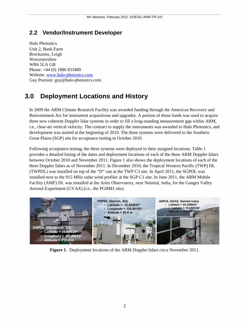
In 2009 the ARM Climate Research Facility was awarded funding through the American Recovery and Reinvestment Act for instrument acquisitions and upgrades. A portion of those funds was used to acquire three new coherent Doppler lidar systems in order to fill a long-standing measurement gap within ARM, i.e., clear-air vertical velocity. The contract to supply the instruments was awarded to Halo Photonics, and development was started at the beginning of 2010. The three systems were delivered to the Southern Great Plains (SGP) site for acceptance testing in October 2010.

Following acceptance testing, the three systems were deployed to their assigned locations. Table 1 provides a detailed listing of the dates and deployment locations of each of the three ARM Doppler lidars between October 2010 and November 2011. Figure 1 also shows the deployment locations of each of the three Doppler lidars as of November 2011. In December 2010, the Tropical Western Pacific (TWP) DL (TWPDL) was installed on top of the “D” van at the TWP C3 site. In April 2011, the SGPDL was installed next to the 915 MHz radar wind profiler at the SGP C1 site. In June 2011, the ARM Mobile Facility (AMF) DL was installed at the Aries Observatory, near Nainital, India, for the Ganges Valley Aerosol Experiment (GVAX) (i.e., the PGHM1 site).

Figure 1. Deployment locations of the ARM Doppler lidars circa November 2011.

http://www.halo-photonics.com/


3

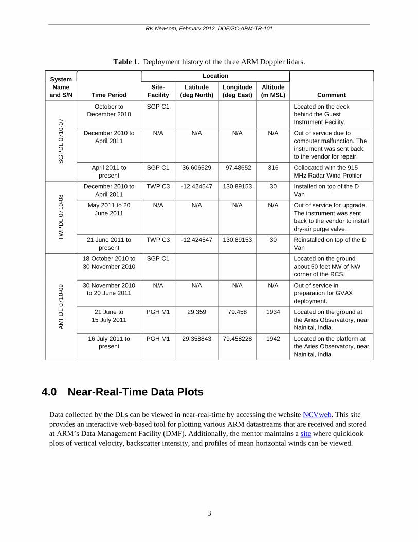
Table 1. Deployment history of the three ARM Doppler lidars.

System Name

and S/N Time Period

Location

Comment Site-

Facility Latitude

(deg North) Longitude (deg East)

Altitude (m MSL)

SG

PD

L 07

10-0

7

October to December 2010

SGP C1 Located on the deck behind the Guest Instrument Facility.

December 2010 to April 2011

N/A N/A N/A N/A Out of service due to computer malfunction. The instrument was sent back to the vendor for repair.

April 2011 to present

SGP C1 36.606529 -97.48652 316 Collocated with the 915 MHz Radar Wind Profiler

TWP

DL

0710

-08

December 2010 to April 2011

TWP C3 -12.424547 130.89153 30 Installed on top of the D Van

May 2011 to 20 June 2011

N/A N/A N/A N/A Out of service for upgrade. The instrument was sent back to the vendor to install dry-air purge valve.

21 June 2011 to present

TWP C3 -12.424547 130.89153 30 Reinstalled on top of the D Van

AM

FDL

0710

-09

18 October 2010 to 30 November 2010

SGP C1 Located on the ground about 50 feet NW of NW corner of the RCS.

30 November 2010 to 20 June 2011

N/A N/A N/A N/A Out of service in preparation for GVAX deployment.

21 June to 15 July 2011

PGH M1 29.359 79.458 1934 Located on the ground at the Aries Observatory, near Nainital, India.

16 July 2011 to present

PGH M1 29.358843 79.458228 1942 Located on the platform at the Aries Observatory, near Nainital, India.

4.0 Near-Real-Time Data Plots

Data collected by the DLs can be viewed in near-real-time by accessing the website NCVweb. This site provides an interactive web-based tool for plotting various ARM datastreams that are received and stored at ARM’s Data Management Facility (DMF). Additionally, the mentor maintains a site where quicklook plots of vertical velocity, backscatter intensity, and profiles of mean horizontal winds can be viewed.

http://plot.dmf.arm.gov/ncvweb/ncvweb.cgi

https://engineering.arm.gov/~newsom


4

5.0 Data Description and Examples

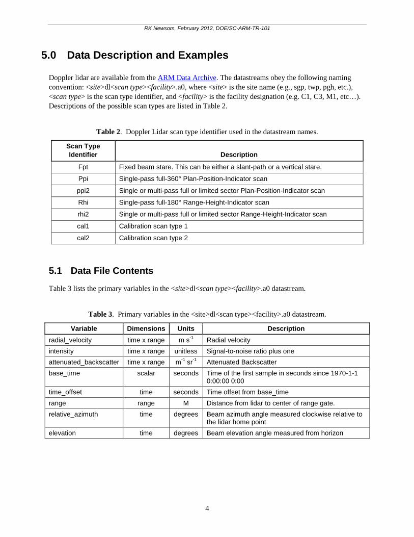
Doppler lidar are available from the ARM Data Archive. The datastreams obey the following naming convention: <site>dl<scan type><facility>.a0, where <site> is the site name (e.g., sgp, twp, pgh, etc.), <scan type> is the scan type identifier, and <facility> is the facility designation (e.g. C1, C3, M1, etc…). Descriptions of the possible scan types are listed in Table 2.

Table 2. Doppler Lidar scan type identifier used in the datastream names.

Scan Type Identifier Description

Fpt Fixed beam stare. This can be either a slant-path or a vertical stare.

Ppi Single-pass full-360° Plan-Position-Indicator scan

ppi2 Single or multi-pass full or limited sector Plan-Position-Indicator scan

Rhi Single-pass full-180° Range-Height-Indicator scan

rhi2 Single or multi-pass full or limited sector Range-Height-Indicator scan

cal1 Calibration scan type 1

cal2 Calibration scan type 2

5.1 Data File Contents

Table 3 lists the primary variables in the <site>dl<scan type><facility>.a0 datastream.

Table 3. Primary variables in the <site>dl<scan type><facility>.a0 datastream.

Variable Dimensions Units Description radial_velocity time x range m s-1 Radial velocity intensity time x range unitless Signal-to-noise ratio plus one attenuated_backscatter time x range m-1 sr-1 Attenuated Backscatter base_time scalar seconds Time of the first sample in seconds since 1970-1-1

0:00:00 0:00 time_offset time seconds Time offset from base_time range range M Distance from lidar to center of range gate. relative_azimuth time degrees Beam azimuth angle measured clockwise relative to

the lidar home point elevation time degrees Beam elevation angle measured from horizon

http://www.archive.arm.gov/


5

5.2 Annotated Examples

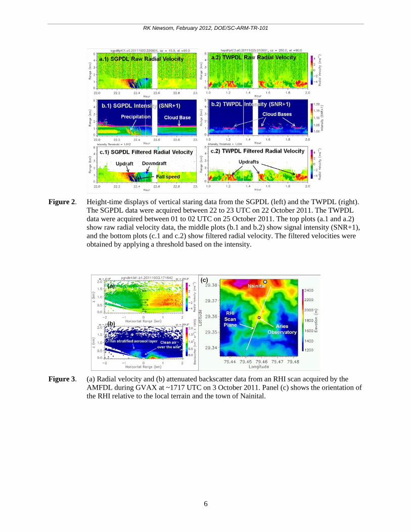
Figures 2 through 4 show annotated examples of data products from the ARM DLs. Figure 2 shows examples of vertical staring data from the SGPDL and the TWPDL. Figure 3 shows a representative example of a range-height indicator (RHI) scan from the AMFDL during GVAX, and Figure 4 shows a time-height cross-section of the mean wind speed and direction derived from SGPDL plan-position indicator (PPI) scan data.

The left side of Figure 2 shows time-height cross-sections of vertical velocity and backscatter intensity (SNR+1) from the SGPDL. This particular example was taken from a period of thunderstorm activity between 22 to 23 UTC on 22 October 2011. The backscatter intensity clearly shows a solid cloud base at about 1.3 km above ground level (AGL). The vertical velocity shows a significant updraft between about 2215 and 2224 UTC. This is immediately followed by an equally strong downdraft that lasts for roughly the same amount of time. Precipitation, which begins during the updraft period, is clearly visible in both the intensity and vertical velocity plots. Vertical velocities from the precipitation stand out in sharp contrast to the clear-air vertical velocities.

The right side of Figure 2 shows time-height cross sections of backscatter intensity and vertical velocity from the TWPDL between 01 and 02 UTC on 25 October 2011. This case corresponds with a very typical afternoon period at the Darwin site. The plots indicate active convection within the boundary layer and the presence of scattered fair-weather cumulus clouds. Cloud bases in this example occur at roughly 1.1 km AGL. One can clearly see the updrafts that occur below cloud bases and the downdrafts that occur during breaks in the clouds.

Figure 3 shows a typical example of radial velocity and backscatter measurements from an RHI scan taken by the AMFDL during GVAX on 3 October 2011. The orientation of the RHI scan relative to the local terrain and the town of Nainital, India, is shown in Figure 3c. The particular example shows a fairly complex vertical structure characterized by thin layers with distinct shifts in either wind speed or wind direction.

Finally, Figure 4 shows a time-height display of the mean horizontal winds derived from the SGPDL for the period from 26 through 28 September 2011. Profiles of the mean winds are derived from hourly PPI scan data using a modified velocity-azimuth display (VAD) algorithm (Banta et al. 2002, Browning et al. 1968). Wind speeds are represented in color, and the flow direction is represented by vectors. Vectors that point upward (downward) correspond to southerly (northerly) flow. This particular example shows the formation and dissipation of nocturnal low-level jets (LLJ), which is a characteristic feature of the Great Plains.


6

Figure 2. Height-time displays of vertical staring data from the SGPDL (left) and the TWPDL (right).

The SGPDL data were acquired between 22 to 23 UTC on 22 October 2011. The TWPDL data were acquired between 01 to 02 UTC on 25 October 2011. The top plots (a.1 and a.2) show raw radial velocity data, the middle plots (b.1 and b.2) show signal intensity (SNR+1), and the bottom plots (c.1 and c.2) show filtered radial velocity. The filtered velocities were obtained by applying a threshold based on the intensity.

Figure 3. (a) Radial velocity and (b) attenuated backscatter data from an RHI scan acquired by the

AMFDL during GVAX at ~1717 UTC on 3 October 2011. Panel (c) shows the orientation of the RHI relative to the local terrain and the town of Nainital.


7

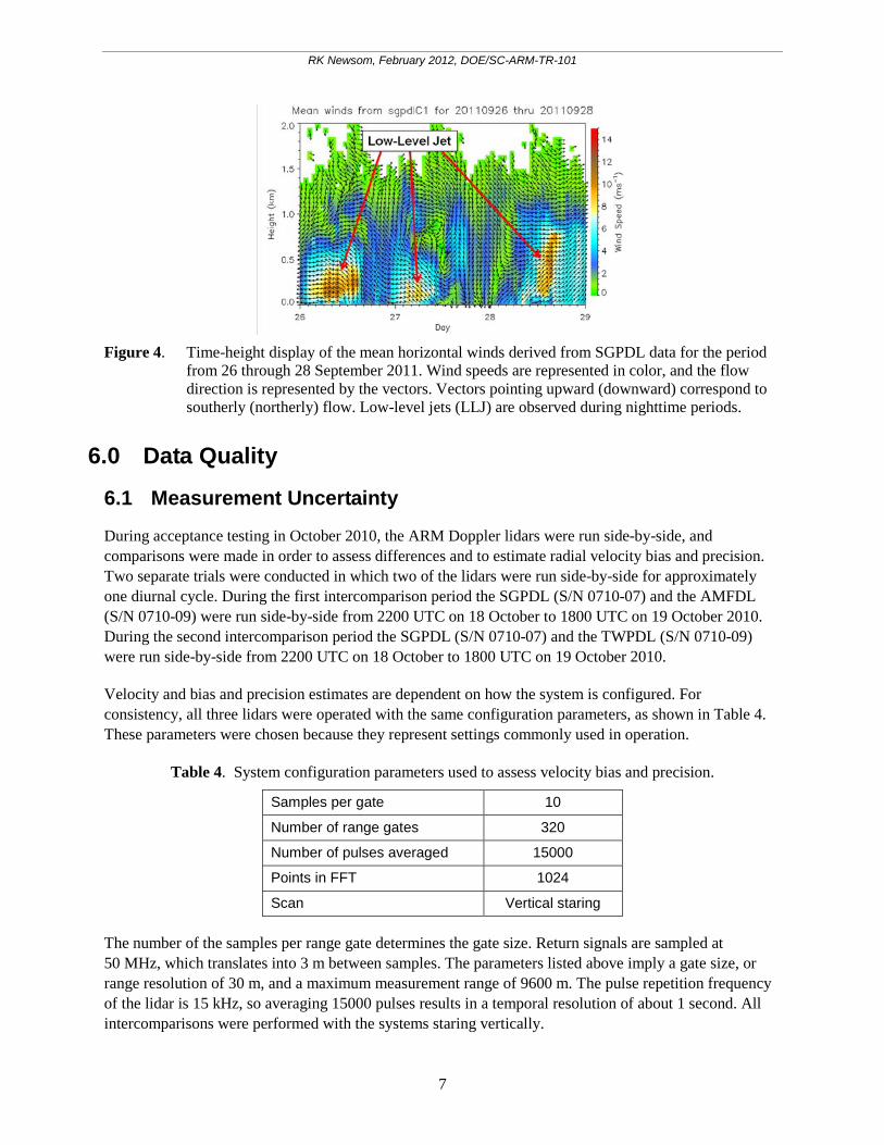
Figure 4. Time-height display of the mean horizontal winds derived from SGPDL data for the period

from 26 through 28 September 2011. Wind speeds are represented in color, and the flow direction is represented by the vectors. Vectors pointing upward (downward) correspond to southerly (northerly) flow. Low-level jets (LLJ) are observed during nighttime periods.

6.0 Data Quality

6.1 Measurement Uncertainty

During acceptance testing in October 2010, the ARM Doppler lidars were run side-by-side, and comparisons were made in order to assess differences and to estimate radial velocity bias and precision. Two separate trials were conducted in which two of the lidars were run side-by-side for approximately one diurnal cycle. During the first intercomparison period the SGPDL (S/N 0710-07) and the AMFDL (S/N 0710-09) were run side-by-side from 2200 UTC on 18 October to 1800 UTC on 19 October 2010. During the second intercomparison period the SGPDL (S/N 0710-07) and the TWPDL (S/N 0710-09) were run side-by-side from 2200 UTC on 18 October to 1800 UTC on 19 October 2010.

Velocity and bias and precision estimates are dependent on how the system is configured. For consistency, all three lidars were operated with the same configuration parameters, as shown in Table 4. These parameters were chosen because they represent settings commonly used in operation.

Table 4. System configuration parameters used to assess velocity bias and precision.

Samples per gate 10

Number of range gates 320

Number of pulses averaged 15000

Points in FFT 1024

Scan Vertical staring

The number of the samples per range gate determines the gate size. Return signals are sampled at 50 MHz, which translates into 3 m between samples. The parameters listed above imply a gate size, or range resolution of 30 m, and a maximum measurement range of 9600 m. The pulse repetition frequency of the lidar is 15 kHz, so averaging 15000 pulses results in a temporal resolution of about 1 second. All intercomparisons were performed with the systems staring vertically.


8

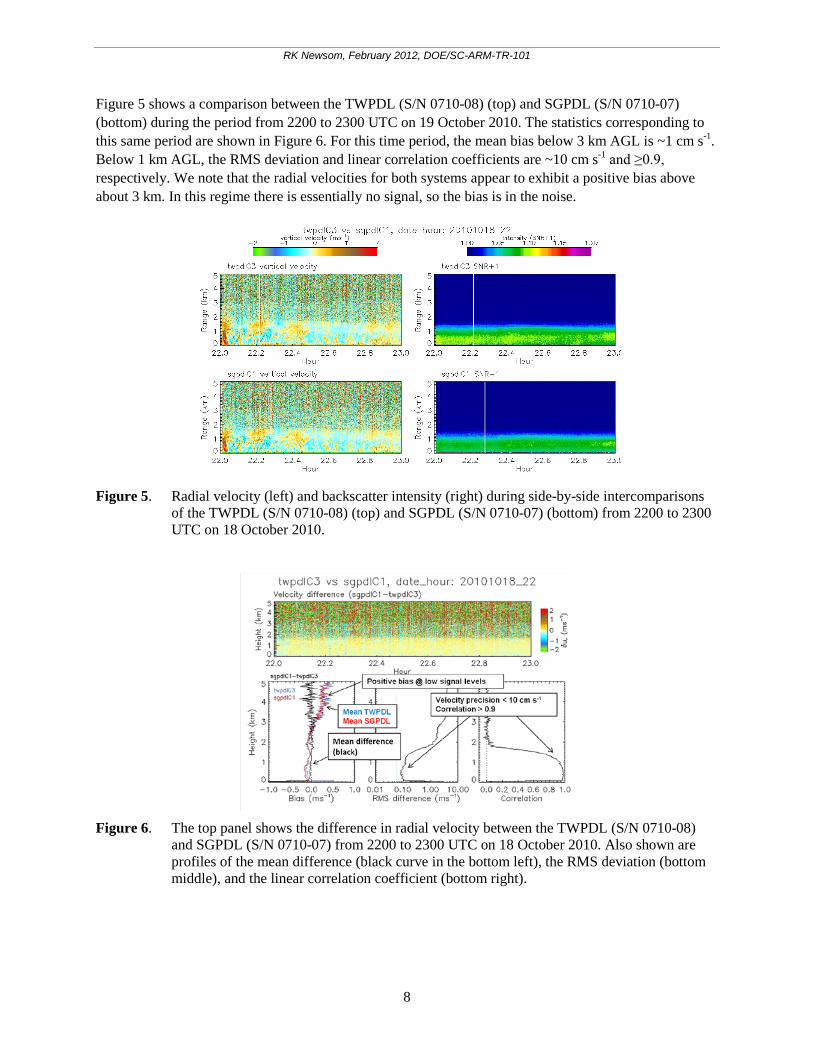
Figure 5 shows a comparison between the TWPDL (S/N 0710-08) (top) and SGPDL (S/N 0710-07) (bottom) during the period from 2200 to 2300 UTC on 19 October 2010. The statistics corresponding to this same period are shown in Figure 6. For this time period, the mean bias below 3 km AGL is ~1 cm s-1. Below 1 km AGL, the RMS deviation and linear correlation coefficients are ~10 cm s-1 and ≥0.9, respectively. We note that the radial velocities for both systems appear to exhibit a positive bias above about 3 km. In this regime there is essentially no signal, so the bias is in the noise.

Figure 5. Radial velocity (left) and backscatter intensity (right) during side-by-side intercomparisons

of the TWPDL (S/N 0710-08) (top) and SGPDL (S/N 0710-07) (bottom) from 2200 to 2300 UTC on 18 October 2010.

Figure 6. The top panel shows the difference in radial velocity between the TWPDL (S/N 0710-08)

and SGPDL (S/N 0710-07) from 2200 to 2300 UTC on 18 October 2010. Also shown are profiles of the mean difference (black curve in the bottom left), the RMS deviation (bottom middle), and the linear correlation coefficient (bottom right).


9

Estimates of velocity precision were also made during the intercomparison periods. The velocity precision is defined as the standard deviation of the measurement noise. The noise level is estimated from the difference between the zeroth and first lags of the autocovariance function (ACF) of the radial velocity time-series at a fixed range gate (Frehlich 2001).The autovariance function is given by

∑−−

=+ −−

−=

iN

kjjkijjiij wwww

iNACF

1

0,, ))((1

(1)

where jiw , is the radial velocity at time it and range jr . The mean radial velocity at range jr is denoted

by jw . The velocity precision is then estimated to be

2/110 )( jjj ACFACF −≈∆ (2)

The velocity precision is parameterized in terms of the mean signal-to-noise ratio (SNR) at range , jr i.e.

∑−

=

=1

0

1 N

iijj SNR

NSNR (3)

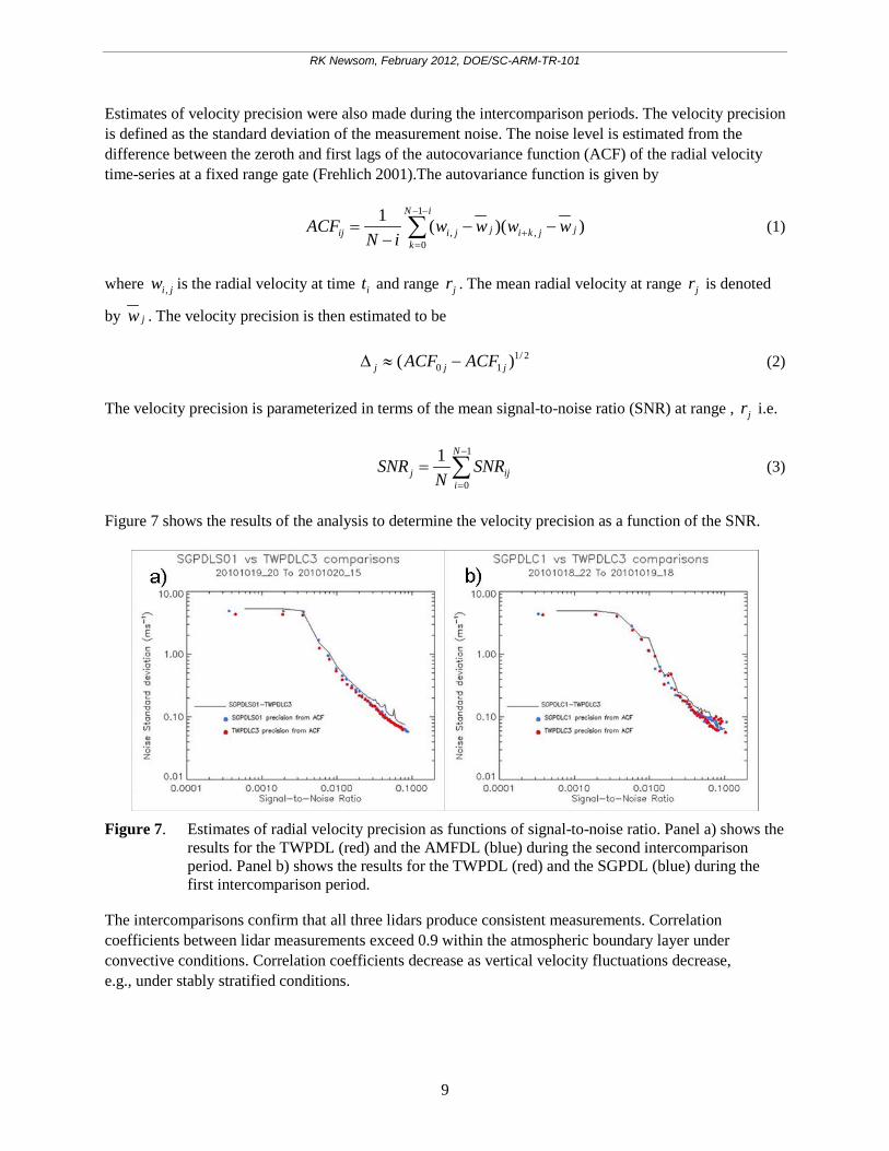
Figure 7 shows the results of the analysis to determine the velocity precision as a function of the SNR.

Figure 7. Estimates of radial velocity precision as functions of signal-to-noise ratio. Panel a) shows the

results for the TWPDL (red) and the AMFDL (blue) during the second intercomparison period. Panel b) shows the results for the TWPDL (red) and the SGPDL (blue) during the first intercomparison period.

The intercomparisons confirm that all three lidars produce consistent measurements. Correlation coefficients between lidar measurements exceed 0.9 within the atmospheric boundary layer under convective conditions. Correlation coefficients decrease as vertical velocity fluctuations decrease, e.g., under stably stratified conditions.


10

Estimates of velocity precision are less than 10 cm s-1 at high SNR and generally less than 20 cm s-1 within the atmospheric boundary layer (below ~2km). All three systems tend to show a positive bias in radial velocity at very low SNR. The magnitude of this bias appears to be system-dependent and can exceed 1.0 m s-1

6.2 Data Quality Health and Status

The Data Quality Office (DQO) website has links to tools for inspecting and assessing raw Doppler lidar data quality:

• DQ Explorer (Data Quality Explorer)

• NCVweb (Interactive web-based tool for viewing ARM data)

6.3 Data Reviews by Instrument Mentor

The instrument mentor conducts comprehensive data reviews monthly in conjunction with the generation of the Instrument Mentor Monthly Status (IMMS) report. The IMMS reports can be accessed by going to the instrument web page.

6.4 Data Assessments by Site Scientist/Data Quality Office

All DQ Office and most Site Scientist techniques for checking have been incorporated within DQ Explorer and can be viewed there.

7.0 Value-Added Products

There are currently no value-added products (VAPs) being generated operationally. However, the mentor has implemented a modified velocity-azimuth-display (VAD) algorithm for processing PPI scan data. The VAD algorithm generates vertical profiles of the mean horizontal wind speed and direction.

Quicklook plots of the VAD results can be viewed at https://engineering.arm.gov/~newsom/. Efforts are underway to implement the VAD algorithm as a VAP. Additionally, plans are underway to develop and implement an algorithm for computing vertical velocity statistics.

8.0 Instrument Details

8.1 Detailed Description

8.1.1 List of Components

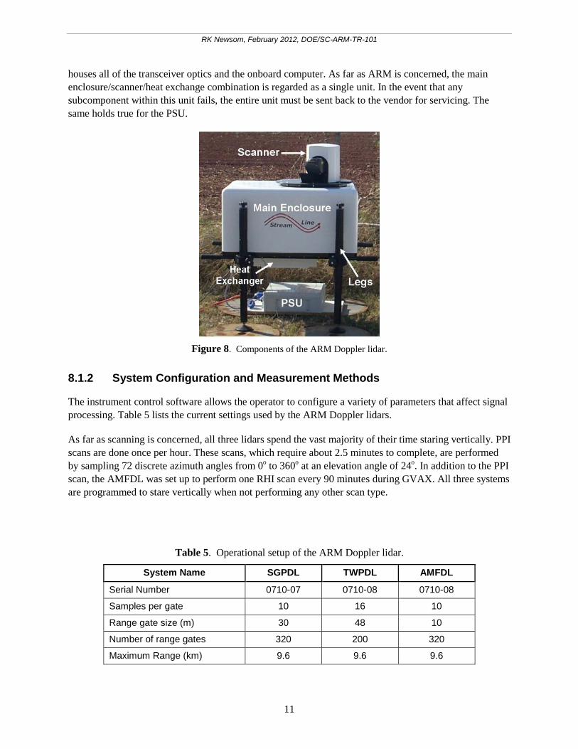
The major components of the ARM Doppler lidars consist of the main enclosure, the scanner, the heat exchanger, telescoping legs, and the power supply unit (PSU), as shown in Figure 8. The main enclosure

http://dq.arm.gov/

http://dq.arm.gov/dq-explorer/cgi-bin/main

http://plot.dmf.arm.gov/ncvweb/ncvweb.cgi

http://www.arm.gov/instruments/dl

http://dq.arm.gov/

http://dq.arm.gov/

https://engineering.arm.gov/~newsom/


11

houses all of the transceiver optics and the onboard computer. As far as ARM is concerned, the main enclosure/scanner/heat exchange combination is regarded as a single unit. In the event that any subcomponent within this unit fails, the entire unit must be sent back to the vendor for servicing. The same holds true for the PSU.

Figure 8. Components of the ARM Doppler lidar.

8.1.2 System Configuration and Measurement Methods

The instrument control software allows the operator to configure a variety of parameters that affect signal processing. Table 5 lists the current settings used by the ARM Doppler lidars.

As far as scanning is concerned, all three lidars spend the vast majority of their time staring vertically. PPI scans are done once per hour. These scans, which require about 2.5 minutes to complete, are performed by sampling 72 discrete azimuth angles from 0o to 360o at an elevation angle of 24o. In addition to the PPI scan, the AMFDL was set up to perform one RHI scan every 90 minutes during GVAX. All three systems are programmed to stare vertically when not performing any other scan type.

Table 5. Operational setup of the ARM Doppler lidar.

System Name SGPDL TWPDL AMFDL

Serial Number 0710-07 0710-08 0710-08

Samples per gate 10 16 10

Range gate size (m) 30 48 10

Number of range gates 320 200 320

Maximum Range (km) 9.6 9.6 9.6


12

Number of pulses averaged 15000 15000 15000

Dwell Time 1 sec 1 sec 1 sec

Points in FFT 1024 1024 1024

8.1.3 Specifications

Performance specifications of the ARM Doppler lidars are presented in Table 6. These instruments employ an eye-safe solid-state laser transmitter operating at a wavelength of 1.5 µm, low pulse energy (~100µJ), and high pulse repetition frequency (15 kHz). These instruments have full upper hemispherical scanning capability and provide range-resolved measurements of attenuated aerosol backscatter and radial velocity, i.e., the velocity component parallel to the beam. Control over the Doppler lidar is facilitated through a connection to the onboard computer. The onboard instrument control software allows the operator to adjust many system parameters and set up various scans. Further details are given by Pearson et al. (2002 and 2009).

Table 6. Specifications for the ARM Doppler lidars.

Manufacturer Halo Photonics Eye safety Class 1M Wavelength 1.5 µm Laser pulse energy ~100 µJ Laser pulse width 150 ns (22.5 m) Pulse rate 15 kHz Nyquist Velocity 19.4 ms-1 Unambiguous range 10 km Aperture 75 mm Volume approximately 0.5 m3 Power consumption < 300 W Mass approximately 85Kg Temporal resolution selectable from 0.1 to 30 seconds Range gate size 18 to 60m Velocity precision < 20 cm s-1

for SNR > -17 dB

Minimum range <100m, typically 75m Scanning Step-stare, full upper hemisphere Enclosure Weatherproof, temperature stabilized

8.2 Theory of Operation

The ARM Doppler lidars employ a monostatic design, in which pulses of highly columnated laser radiation are transmitted into the atmosphere. The laser operates at the near-IR wavelength of =oλ 1.5

µm. As the radiation propagates through the atmosphere, it is scattered by aerosol and cloud particles (molecular scattering is very weak in this wavelength regime). Backscattered radiation is collected by the transceiver and processed to generate estimates of radial velocity and attenuated backscatter. In general,


13

the backscattered radiation experiences a Doppler shift that depends on the light-of-sight (radial) velocity of the scatterers relative to the lidar. A “red” shift occurs if the scatterers are moving away from the lidar, and a “blue” shift occurs if the scatterers are moving toward the lidar.

The Doppler shift of the backscattered radiation is quite small relative the outgoing pulse. As an example, a wind velocity of 30 ms-1 would result in a Doppler shift of only 10 MHz on at 1.5 μm. This amounts to a shift of 50 ppb relative to the optical frequency of 200 THz. Nevertheless, it is possible to measure such small shifts with very good precision using heterodyne detection.

In coherent Doppler lidar, heterodyning is achieved by mixing the backscattered radiation with light from a frequency-stable continuous-wave laser, i.e., the so-called local oscillator (LO). The mixed signal exhibits a temporal modulation in the amplitude that oscillates at the frequency difference between the two beams. This is the signal that is detected, and the modulation frequency indicates the Doppler shift (Grund et al. 2001).

As an example, we assume a simple monochromatic backscattered field given by

( )φω += tAE cos (4)

where A is the amplitude, ω is the angular frequency, t is time, and φ is an arbitrary phase. The frequency ω is given by the known frequency of the outgoing pulse oω plus a small Doppler shift

Dopplerδω , i.e.

Dopplero δωωω += (5)

The local oscillator field is similarly represented as

( )LOLOLOLO tAE φω += cos (6)

where LOω is the known LO frequency.

In coherent detection the backscattered light and the LO are superimposed by optically combining and co-propagating the beams inside the transceiver. The combined beam is then directed onto a photo detector, which generates a signal in response the irradiance. The irradiance at the photo detector is given by

( ) ( ) ( )φωφω ∆+∆++++=+∝ ++ tAAtAAEEEEI LOLOLOLOH coscos222 (7)

where LOωωω +=+ , LOφφφ +=+ , LOωωω −=∆ , and LOφφφ −=∆ . The first three terms on the right-hand side of equation (7) oscillate at optical frequencies (100s of THz). These rapidly oscillating fields fall well outside of the photo detector’s pass band. The last term in equation (7) oscillates at the difference frequency LOωωω −=∆ , which is typically on the order of 10 MHz and well within the detector’s pass band. Thus, the signal coming off the photo-detector can be written as


14

( )φω ∆+∆∝ tts cos)( (8)

where

LOoDopplerLO ωωδωωωω −+=−=∆ (9)

Equation (8) represents the raw heterodyne signal that is detected. By knowing the frequency difference, if any, between the outgoing pulse and the local oscillator, it is possible to determine the Doppler shift of the backscattered radiation from an analysis of the Fourier transform of the raw heterodyne signal (Rye and Hardesty 1993a,1993b; Frehlich 1999). In practice, the raw signal is first downmixed to baseband and then digitized at an appropriate sampling rate. In the case of the ARM Doppler lidars, the raw signals are downmixed and sampled at 50MHz; thus, the receiver bandwidth is ±25MHz, which gives a Nyquist velocity of about 19 ms-1.

Real-time signal processing is a key aspect of the Doppler lidar. The signal processing unit handles gating of the raw signal, autovariance computations, accumulation, and Doppler frequency estimation. The time-resolved (and downmixed) heterodyne signal from a single laser pulse echo is subdivided, or gated, into a number of contiguous range bins. The complex autocovariance function for each range bin is computed and then accumulated over a user-specified number of laser pulses, pulseN . After pulseN pulses have been

processed in this manner, the Doppler frequency shift is estimated for each range bin. This is accomplished by computing the discrete Fourier transform of the accumulated autovariance functions and then locating the peaks in the resulting power spectra. The result of this computation produces estimates of Dopplerδω for each range bin.

Doppler shift estimates are converted to radial velocity using

πδωλ 4/Doppleroru −= (10)

where =oλ 1.5 µm is the wavelength of the outgoing pulse. The negative sign in equation (10) implies that a negative Doppler shift (red shift) results in a positive radial velocity. We note that negative shifts occur when scatterers are moving away from the lidar. This would correspond to a case in which the radial distance between the lidar and the scatterer increases with time, which by definition is a positive velocity.

In addition to radial velocity, the Doppler lidar produces estimates of the wideband signal-to-noise ratio, which by definition is the coherent signal power divided by the noise power in the full bandwidth.

8.3 Calibration

Radial velocities require no calibration.


15

8.4 Operation and Maintenance

8.4.1 User Manual

The operations manual is considered proprietary by the vendor. Thus, it is only made available to authorized personnel. Requests for information regarding the operation of the Doppler lidar should be directed to the instrument mentor.

8.4.2 Routine and Corrective Maintenance Documentation

Routine and corrective maintenance documentation is maintained by on-site technicians.

8.5 Glossary

See the ARM Glossary.

8.6 Citable References

Banta RM, RK Newsom, JK Lundquist, YL Pichugina, RL Coulter, and LD Mahrt. 2002. “Nocturnal low-level jet characteristics over Kansas during CASES-99.” Boundary-Layer Meteorology 105: 221–252.

Browning, K, and R Wexler. 1968. “The determination of kinematic properties of a wind field using Doppler radar.” Journal of Applied Meteorology 7: 105–113.

Frehlich, RG. 2001. “Estimation of velocity error for Doppler lidar measurements.” Journal of Atmospheric and Oceanic Technology 18: 1628–1639.

Frehlich, RG. 1999. “Maximum likelihood estimators for Doppler radar and lidar.” Journal of Atmospheric and Oceanic Technology 16: 1702–1709.

Grund, CJ, RM Banta, JL George, JN Howell, MJ Post, RA Richter, and AM Weickmann. 2001. “High-resolution Doppler lidar for boundary layer and cloud research.” Journal of Atmospheric and Oceanic Technology 18: 376–393.

Pearson et al. 2002. “Analysis of the Performance of a Coherent Pulsed Fiber Lidar for Aerosol Backscatter Applications.” Applied Optics 41: 6442–6450.

Pearson, GN, F Davies and C Collier. 2009. “An analysis of the performance of the UFAM pulsed Doppler lidar for observing the boundary layer.” Journal of Atmospheric and Oceanic Technology 26: 240–250.

Rye, BJ, and RM Hardesty. 1993a. “Discrete spectral peak estimation in incoherent backscatter heterodyne lidar. I. Spectral accumulation and the Cramer-Rao lower bound.” IEEE Transactions on Geoscience and Remote Sensing 31: 16–27.

http://www.arm.gov/about/glossary


16

Rye, BJ, and RM Hardesty. 1993b. “Discrete spectral peak estimation in incoherent backscatter heterodyne lidar. II. Correlogram accumulation.” IEEE Transactions on Geoscience and Remote Sensing 31: 28–35.

Werner, C. 2005. “Doppler wind lidar. Lidar: Range-Resolved Optical Remote Sensing of the Atmosphere.” C Weitkamp, Ed., Series in Optical Sciences 102: Springer, 339–342.

DISCLAIMER - ARM Climate Research Facility AMF Doppler Lidar . ARM Atmospheric Radiation Measurement...

Documents

Transcript of DISCLAIMER - ARM Climate Research Facility AMF Doppler Lidar . ARM Atmospheric Radiation Measurement...