Disasters, Recoveries, and Predictability

François Gourio�

April 2008

Abstract

I review the disaster explanation of the equity premium puzzle, discussed in Barro (2006) and

Rietz (1988). In the data, disasters are often followed by recoveries. I study how recoveries a¤ect

the implications of the model. This turns out to depend heavily on the elasticity of intertemporal

substitution (IES). For a high IES, the disaster model does not generate a sizeable equity premium.

I also study whether the disaster model can �t the time-series evidence on predictability of stock

returns, as argued by Gabaix (2007). I �nd that the model has di¢ culties matching these facts.

Finally, I propose a cross-sectional test of the disaster model: assets which do better in disasters

should have lower average returns. There seems to be little evidence supporting this prediction.

1 Introduction

Twenty years ago, Thomas A. Rietz (1988) showed that infrequent, large drops in consumption make

the theoretical equity premium large. Recent research has resurrected this �disaster�explanation of the

equity premium puzzle. Robert J. Barro (2006) measures disasters during the XXth century, and �nds

that they are frequent and large enough, and stock returns low enough relative to bond returns during

disasters, to make this explanation quantitatively plausible. Xavier Gabaix (2007) extends the model

to incorporate a time-varying incidence of disasters, and he argues that this simple feature can resolve

many asset pricing puzzles.1

This paper reviews the disaster-based explanations and adds to the debate in three dimensions.

First, all the papers in this literature assume that disasters are permanent. Mathematically, they model

log consumption per capita as the sum of a unit root process and a Poisson jump. However a casual look

at the data suggests that disasters are often followed by recoveries. The �rst contribution of this paper

is to measure recoveries and introduce recoveries in the Barro-Rietz model. In doing so, I follow Barro�s

suggestion that �a worthwhile extension would deal more seriously with the dynamics of crisis regimes�

�This paper merges three short papers of mine: �Disasters and recoveries� (AER P&P May 2008), �Time-series pre-

dictability in the disaster model�, and �A cross-sectional test of the disaster model�. I thank Robert Barro, John Campbell,

Xavier Gabaix, Ian Martin, Romain Ranciere, and Adrien Verdelhan for discussions or comments. Contact information:

Boston University, Department of Economics, 270 Bay State Road, Boston MA 02215. Email: fgourio@bu.edu. Tel.: (617)

353 4534.1The literature is growing rapidly, e.g. see Farhi and Gabaix (2007) for an application to the forward premium puzzle,

and Martin (2008) for a nonparametric formulation.

1

(p. 854). I �nd that the e¤ect of recoveries hinges on the intertemporal elasticity of substitution (IES):

when the IES is low, recoveries may increase the equity premium implied by the model; but when it

is high, the opposite happens. Hence, recoveries can have a powerful e¤ect on the implications of this

model. The implications for the pattern of P-D ratios and risk-free rates during disasters are however

challenging.

My second contribution is to study if the disaster model can account for the time-series predictability

of stock returns. I show theoretically that the model with a time-varying probability of disaster cannot

account for the �ndings of stock return and excess stock return predictability, if utility is CRRA,

regardless of the parameter values. Even using an Epstein-Zin utility function does not seem to help

quantitatively much.

Finally, I study a natural cross-sectional implication: assets which do well during disasters should

have low average (or expected) returns. I test this implication using as assets a variety of stocks, sorted

by industries, size, and other variables, for the United States during the XXth century. I �nd little

support for this idea - exposures to disasters are not signi�cantly correlated with average returns.

Collectively these �ndings raise signi�cant challenges for the disaster model. In particular, there is a

tension between the need for a high IES to reduce the volatility of risk-free interest rates, and the need

for a low IES to reduce the e¤ect of recoveries.

The rest of the paper is organized as follows. Section 2 presents the simple disaster model. Section

3 quanti�es the importance of recoveries in the data and in the model. Section 4 studies if the disaster

model can account for time-variation in equity return and risk premia, and Section 5 studies the cross-

sectional implications of the disaster model.

2 The Disaster model: a review

The Barro-Rietz model is a variant of the familiar Lucas tree asset pricing model. There is a represen-

tative agent with power utility:

E1Xt=0

�tC1� t

1� :

Barro and Rietz assume the following consumption process:

� logCt = �+ �"t; with probability 1� p;

= �+ �"t + log(1� b); with probability p;

where "t is iid N(0; 1): Hence, each period, with probability p, consumption drops by a factor b, e.g.

b = 40%: The realization of the disaster is iid and statistically independent of the �business cycle risk�

"t at all dates. Because risk-averse agents fear large changes in consumption, a small probability of a

large drop of consumption can make the theoretical equity premium large.

In this model, the P-D ratio is constant, since the consumption growth process is iid and utility is

CRRA. We have the following expression for the risk-free and for the equity premium:

logRf = � log � + �� 2�2

2� log

�1� p+ p(1� b)�

�;

2

log

�ERe

Rf

�= �2 + log

�(1� p+ p(1� b)) (1� p+ p(1� b)� )

1� p+ p(1� b)1�

�:

When p = 0; these formulas lead to the standard results of the iid lognormal model. When disasters

are possible, i.e. p > 0; we see that the risk-free rate is lower, and the equity premium is higher.

I �rst follow Barro�s calibration to illustrate the potential of this model to account for the equity

premium puzzle. Barro uses standard values for the trend growth �, the standard deviation of business

cycle shocks � and the discount rate �: � = 0:02; � = 0:025; � = 0:97: He sets risk aversion equal

to = 4, which implies an intertemporal elasticity of substitution of 1=4: Finally, the probability of

a disaster in a given year is p = 0:017, and the disaster size b is actually random: b is drawn from

the historical distribution of disasters, as measured by Barro (see the next section).2 These parameter

values leads to an arithmetic equity premium E�Re �Rf

�equal to 5.6%. By contrast, without the

disasters, the equity premium would be only 0.18%.

Government bonds are not risk-free in disasters. Barro argues that a reasonable calibration is that,

during disasters, bonds repay with probability 0:6 the full amount and with probability 0:4 repay a

fraction 1 � b: Taking this into account reduces the risk premium to 3.5%. (Barro also studies how

leverage may increase this number, and how survivorship bias may a¤ect our estimates of the equity

premium.) These numbers are driven by the very extreme disasters. For instance, if we consider only

the disasters which are less than 40% (which all occurred during World War II), the equity premium is

reduced to 0.8%.3

The disaster model has a constant P-D ratio, because disasters are iid: Hence it cannot address the

stock market volatility puzzle or the time-series predictability puzzle. However, a natural extension is to

make the probability of disasters p, or perhaps the size of disasters b, a stochastic process. Presumably,

when investors�expectations of b and p change, asset prices will move, generating changes over time in

the risk-free rate, the equity premium and the P-D ratio. This extension is studied in Section 4.

3 Disasters and Recoveries

I start by presenting the measure of disasters introduced by Barro (2006) and by measuring recoveries.

Then I extend the Barro-Rietz model to incorporate recoveries, and I discuss the implications.

3.1 Measuring Recoveries

Barro measures disasters as the total decline in GDP from peak to through. Using 35 countries (20

OECD countries and 15 countries from Latin America and Asia), he �nds 60 episodes of GDP declines

greater than 15% during the XXth century. These episodes are concentrated on World War I, the Great

Depression, and World War II, but there is also a signi�cant number of disasters in Latin America since

World War II. The mean decline is 29%. Figure 1 plots log GDP per capita for four countries (Germany,

Netherlands, the U.S., and Chile), and �gure 2 shows the data for Mexico, Peru, Urugay and Venezuela.

2This modi�es slightly the formulas above: an expectation over the disaster size b, conditional on a disaster occuring,

must be added to the formulas.3This extreme sensitivity to extreme events with tiny probability is emphasized by Martin (2008).

3

1900 1920 1940 1960 1980 2000

8

8.5

9

9.5

Germany

1900 1920 1940 1960 1980 2000

8

8.5

9

9.5

Netherlands

1900 1920 1940 1960 1980 2000

8.5

9

9.5

10

U.S.

1900 1920 1940 1960 1980 2000

8

8.5

9

Chile

Figure 1: Log GDP per capita (in 1990 dollars) for four countries: Germany, Netherlands, the U.S. and

Chile. The disaster start (resp.end) dates are taken from Barro (2006), and are shown with a vertical

full (resp. dashed) line.

The vertical full lines indicate the start of disasters, and the vertical dashed lines the end of disasters, as

de�ned by Barro.4 In many cases, GDP bounces back just after the end of the disaster, as predicted by

the neoclassical growth model following a capital destruction or a temporary decrease in productivity.5

To quantify the magnitude of recoveries, Table 1 present some statistics using the entire sample of

disasters6 identi�ed by Barro. Because Barro de�nes disasters such that the end of the disaster is the

trough, this computation implies that GDP goes up following the disaster. The key question is, How

much?

The �rst column reports the average across countries of the cumulated growth, in each of the �rst

�ve years following a disaster. The average growth rate is 11.1% in the �rst year after a disaster, and

the total growth in the �rst two years amounts to 20.9%. This is of course much higher than the average

growth across these countries over the entire sample, which is just 2.0%. The second column computes

how much of the �gap�from peak to trough is resorbed by this growth, i.e. how much lower is GDP

per capita compared to the previous peak. At the trough, on average GDP is 29.8% less than at the

previous peak. But on average, this gap is reduced after three years to 13.7%.

Of particular interest are the larger disasters, because diminishing marginal utility implies that

people care enormously about them (e.g., in the basic disaster model, a .2% probability of a 20%

disaster yields an equity premium of 0.5%, but a 1% probability of a 40% disaster yield an equity

premium of 1.8%) Columns 3 and 4 replicate these computations for the subsample of disasters larger

4The data is from Maddison (2003).5See however Cerra and Saxena (2007) for a di¤erent view.6Except the most recent episodes in Argentina, Indonesia and Urugay, for which the next �ve years of data are not yet

available.

4

1900 1920 1940 1960 1980 2000

7.4

7.6

7.8

8

8.2

8.4

8.6

8.8

Mexico

1900 1920 1940 1960 1980 2000

6.8

7

7.2

7.4

7.6

7.8

8

8.2

Peru

1900 1920 1940 1960 1980 2000

7.8

8

8.2

8.4

8.6

8.8

9Urugay

1900 1920 1940 1960 1980 2000

7

7.5

8

8.5

9

Venezuela

Figure 2: Log GDP per capita (in 1990 dollars) for four countries: Mexico, Peru, Urugay and Venezuela.

The disaster start (resp.end) dates are taken from Barro (2006), and are shown with a vertical full (resp.

dashed) line.

than 25%. These disasters are also substantially reversed, because the average growth in the �rst two

years after the disaster is over 30%. Measuring disasters and recoveries certainly deserves more study,

but it seems clear that the iid assumption is incorrect: growth is substantially larger after a disaster

than unconditionally. (However, recoveries might be less strong for consumption than for GDP if people

are able to smooth consumption during disasters.)

3.2 A Disaster model with Recoveries and Epstein-Zin utility

How do recoveries a¤ect the predictions of the disaster model? To study this question, I extend the

Barro-Rietz model and allow for recoveries. Recall that the consumption process in the Barro-Rietz

model is:

� logCt = �+ �"t; with probability 1� p;

= �+ �"t + log(1� b); with probability p;

where "t is iid N(0; 1): To allow for recoveries, I modify this process as follows: if there was a disaster in

the previous period, then, with probability �; consumption goes back up by an amount � log(1�b): This

is a particularly simple way of modelling recoveries. When � = 0; we have the Barro-Rietz model. When

� = 1, a recovery is certain. Below I consider more complicated (and more realistic) speci�cations.

When � > 0; the consumption process is not iid any more, and as a result the price-dividend ratio

moves over time (more details on this below). There is no useful closed form solution, but the price of

5

In percent All disasters (57 events) Disaster greater than 25% (27 events)

Years Growth Loss from Growth Loss from

after Trough from Trough previous Peak from Trough previous Peak

0 0 -29.8 0 -41.5

1 11.1 -22.8 16.1 -32.7

2 20.9 -16.8 31.3 -24.2

3 26.0 -13.7 38.6 -20.4

4 31.5 -10.2 45.5 -16.9

5 37.7 -6.1 52.2 -13.4

Table 1: Measuring Recoveries. The table reports the average of (a) the growth from the trough to

1,2,3,4,5 years after the trough and (b) the di¤erence from the current level of output to the previous

peak level, for 0,1,2,3,4,5 years after the trough.

equity can still be easily calculated using the standard recursion:

PtCt= Et

e��

�Ct+1Ct

�1� �1 +

Pt+1Ct+1

�!:

I use the same parameter values as Barro (see Section 2). Figure 3 depicts the equity premium, as

a function of the probability � of a recovery. This is a comparison across di¤erent economies which

are identical but for the parameter �. (In particular, I keep the same assumptions as Barro for the

government bond default.) For � = 0 we have, as in Section 3, an equity premium of 3.5%. The equity

premium is higher when the probability of a recovery is higher.

While this result may be surprising at �rst, it is actually easy to understand. Consider the e¤ect on

the price-dividend ratio, right after a disaster, of the possibility of recovery. Start from the present-value

identity: the price of a claim to fCtg satis�es

PtCt= Et

Xk�1

�k�Ct+kCt

�1� ;

hence the fact that a recovery may arise, i.e. that Ct+1; Ct+2; :::; is higher than would have been expected

without a recovery, can increase or decrease the stock price today, depending on whether > 1 or < 1:

The intuition is that good news about the future have two e¤ects: on the one hand, they increase future

dividends ( equal to consumption), which increases the stock price today (the cash-�ow e¤ect), but on

the other hand they increase interest rates, which lowers the stock price today (the discount-rate e¤ect).

The later e¤ect is stronger when interest rates rise more for a given change in consumption, i.e. when

the intertemporal elasticity of substitution (IES) is lower. Given a low IES, the price-dividend ratio

falls more when there is a possible recovery than when there are no recoveries. This in turn means that

equities are more risky ex-ante, and as a result the equity premium is larger.

This discussion clearly suggests that the IES plays a role by a¤ecting risk-free interest rates. While

Barro and Rietz used a low IES, this was merely because they required a signi�cant risk aversion. To

disentangle these two parameters, I extend the model and introduce recursive preferences, as in Epstein

6

0 0.1 0.2 0.3 0.4 0.5 0.6 0.7 0.8 0.9 10

1

2

3

4

5

6

7

8

Probabil ity of recovery (π )

Equi

ty p

rem

ium

 (% p

er y

ear)

Figure 3: This �gure plots the unconditional equity premium, as a function of the probability of recovery

following a disaster, in the CRRA model. Parameters as in Barro (2006).

and Zin (1989). This allows me to compute the predictions of the Barro-Rietz model when risk aversion

is large but the IES is not small. Utility is de�ned through the recursion:

Vt =

��1� e��

�C1��t + e��Et

�V 1��t+1

� 1��1��

� 11��

:

With these preferences, the IES is 1=� and the risk aversion to a static gamble is �: The stochastic

discount factor is:

Mt+1 = e���Ct+1Ct

��� Vt+1

Et(V1��t+1 )

11��

!���;

and it is straightforward to compute the equity premium and government bond price, taking default

into account, with this formula (see the appendix for computational details). Table 2 shows the (log

geometric unconditional) equity premium, as a function of the probability of a recovery, for four di¤erent

elasticities of substitution: 1=4 (Barro�s number), 1=2; 1 and 2: In this computation, the risk aversion �

is kept constant equal to 4: Note that the four lines intersect for � = 0 since in this case, consumption

growth is iid, and the IES does not a¤ect the equity premium.

For an IES= 0:25; we have the results of �gure 3. When the IES is not so low however, recoveries

reduce the equity premium. The intuition is that the decrease in dividends is transitory and thus in

disasters stock prices fall by a smaller amount than dividends do, making equities less risky than in the

iid case. These results are consistent with the literature on autocorrelated consumption growth and

log-normal processes (John Y. Campbell (1999), Ravi Bansal and Amir Yaron (2004)). While Bansal

and Yaron emphasize that the combination of positively autocorrelated consumption growth and an IES

7

Probability of a recovery � 0.00 0.30 0.60 0.90 1.00

IES = 0.25 3.31 4.62 5.91 7.19 7.64

IES = 0.50 3.31 3.30 3.03 2.26 1.68

IES = 1 3.31 2.69 1.94 1.00 0.54

IES = 2 3.31 2.42 1.52 0.63 0.30

Table 2: Unconditional log geometric equity premium, as a function of the intertemporal elasticity

of substitution (IES) and the probability of a recovery. This table sets risk aversion 4 and the other

parameters as in Barro (2006).

above unity can generate large risk premia, Campbell shows that when consumption growth is negatively

autocorrelated, risk premia are larger when the IES is below unity. Recoveries induce negative serial

correlation, so even though Campbell�s results do not directly apply (because the consumption process

is not lognormal), the intuition seems to go through.

Of course, there is no clear agreement on what is the proper value of the IES. The standard view is

that it is small (e.g. Robert Hall (1988)), but this has been challenged by several authors (see among

others Attanasio et al., Bansal and Yaron, Casey Mulligan (2004) Fatih Guvenen (2006), and Vissing

Jorgensen (2001)). How then, can we decide which IES is more reasonable for the purpose of studying

recoveries? The natural answer is to use data on asset prices during disasters.

Implications for asset prices during disasters

How can we decide which IES is more reasonable? The natural solution is to use data on asset prices

during disasters. A low IES implies huge interest rates following a disaster if consumers anticipate a

recovery, while a high IES implies moderately high interest rates, and a small increase in the P-D during

disasters. In the data, interest rates are not huge, but the P-D ratio tends to fall during disasters,

though not necessarily by a large amount. Hence, it is not clear which model �ts the data best. More

fundamentally, in the model, disasters are instantaneous while they are more gradual in the data, making

it di¢ cult to �nd an empirical counterpart to asset prices right after the disaster.

More precisely, �gures 4 and 5 depict the implications of the model with recoveries (� = 1 i.e. no

waiting) for two levels of IES (:25 and 2) and for any probability of recovery. The baseline disaster

model is thus the case where the probability of recovery is zero. The panels present the expected equity

return, risk free rate and risk premium as well as the P-D ratio, conditional on the current state (no

disaster in the previous period, or a 35% disaster just occurred).

These �gures reveal that when the IES is low (the Barro calibration), the possibility of a recovery

has a very large e¤ect on risk-free interest rates following a disasters: as consumers are momentarily

poor, they want to borrow against their future income, which drives the interest rate up. These huge

interest rates are certainly not observed in the data. (Perhaps, people did not anticipate the recoveries.)

The high IES case implies interest rates which are much smaller, because the interest rate does not need

to be so high to make people willing to lend. However, the high IES case also implies that the P-D

ratio increases following a disaster by a moderate amount; compare the bottom panels of Figure 5. In

contrast, the low IES model implies that the P-D ratio falls.

8

0 0.2 0.4 0.6 0.8 14

6

8

10

12No disaster in previous period

Me

an E

quity

 Ret

urn 

(% p

er y

ear

)

IES=.25IES=2

0 0.2 0.4 0.6 0.8 10

100

200

300

400

500Disaster in previous period

IES=.25IES=2

0 0.2 0.4 0.6 0.8 11

1.5

2

2.5

3

3.5

4

4.5

Probability of recovery ( π )

Me

an B

ond 

Re

turn

 (% p

er y

ear)

IES=.25IES=2

0 0.2 0.4 0.6 0.8 10

50

100

150

200

250

300

350

Probability of recovery ( π )

IES=.25IES=2

Figure 4: Asset price implications of the simple example.

0 0.2 0.4 0.6 0.8 10

2

4

6

8No disaster in previous period

Equi

ty P

rem

ium

 (% p

er y

ear)

IES=.25IES=2

0 0.2 0.4 0.6 0.8 10

50

100

150

200Disaster in previous period

IES=.25IES=2

0 0.2 0.4 0.6 0.8 10

10

20

30

40

50

60

Probability of recovery ( π )

P­D

 Rat

io

IES=.25IES=2

0 0.2 0.4 0.6 0.8 10

10

20

30

40

50

60

70

Probability of recovery ( π )

IES=.25IES=2

Figure 5: Asset price implications of the simple example.

9

These results are all driven by the changes in interest rates. The Campbell-Shiller approximation to

the P-D ratio is

logPtDt

= k + (1� �)Et1Xk=1

�k�1�ct+k;

where k is a constant and IES=1=�:7 Hence, future expected growth in consumption (=dividends) will

increase the asset price i¤ � < 1: In the data, we know that P-D ratios fall during disasters, and interest

rates are high, but not on the scale implied by the low IES calibration. Hence, it is not clear which

model �ts the data best. There may be additional elements which a¤ect these results. For instance,

if people become more fearful in disasters (because of high uncertainty or high risk aversion), then the

P-D ratio may fall as the equity premium is large, without having a large e¤ect on the interest rate.

However, this is not easy to make this explanation work quantitatively.

More realistic recovery processes

Clearly the recovery process studied above is too simple: recoveries might not occur right after

a disaster, they sometimes also occur more slowly. Moreover, the size of the recovery is somewhat

uncertain. To take these possibilities into account, I entertain the following Markov chain formulation.

Starting in the normal growth state, with probability p, there is a disaster. Next, with probability �

each period, you stay in a �waiting�state; with 1 � � each period, your recovery is determined: with

probability �1; consumption goes up by � log(1 � b), with probability �2 there is a partial recovery

� log(1� b2); and with probability �3 = 1� �1 � �2 there is no recovery. In any case, you then return

to the �normal state�.

Formally, the Markov matrix is:0BBBBBBBBB@

1� p p 0 0 0

(1� �)�3 0 � (1� �)�1 (1� �)�2(1� �)�3 0 � (1� �)�1 (1� �)�21� p p 0 0 0

1� p p 0 0 0

1CCCCCCCCCA;

where the �rst state is �normal growth�, the second state is the disaster, the third state is the �waiting�

state, and the fourth and �fth state are total or partial recoveries. Note that this formulation assumes

that in states 2 and 3 (i.e. after a disaster and in the waiting period) there is no probability of disaster,

but one can also consider the case where this is possible.8

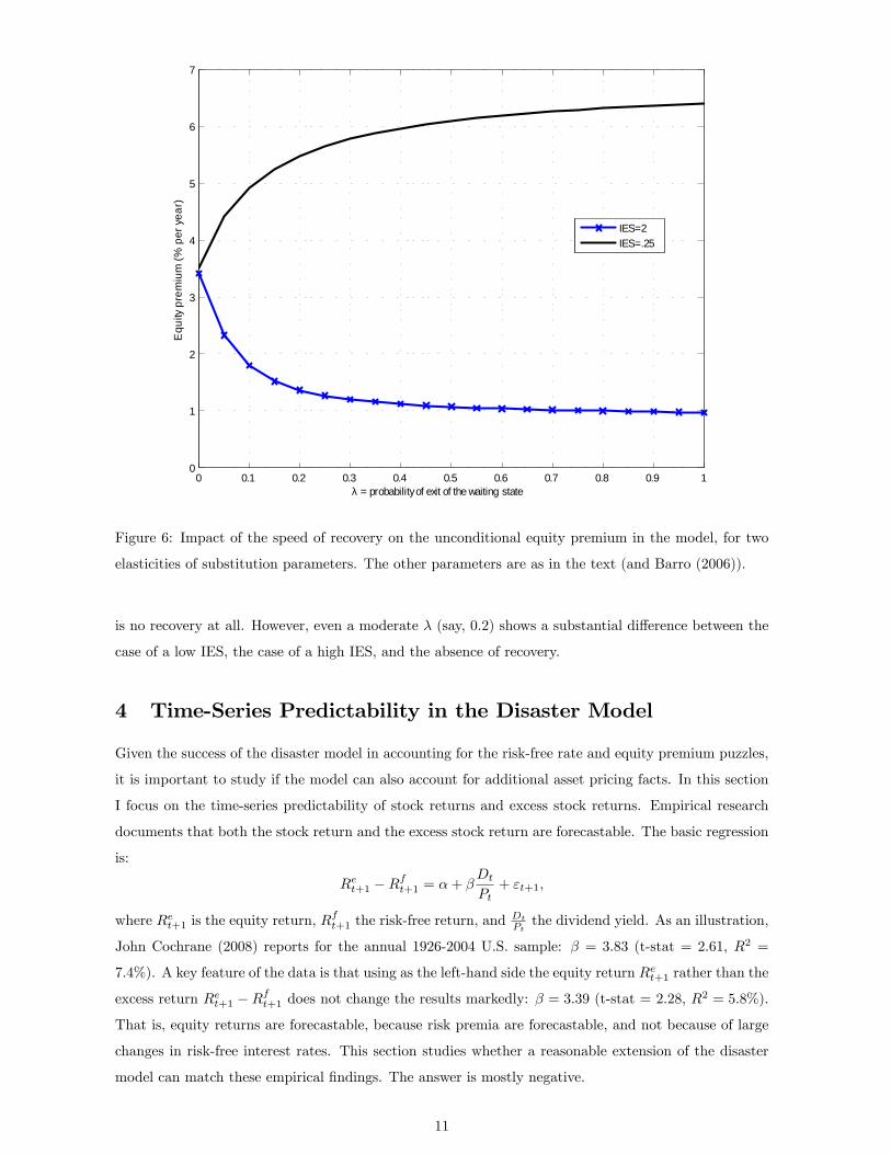
Figure 6 depicts the e¤ect of the speed of convergence on the equity premium. The previous com-

putation implicitly assumed � = 1, i.e. the decision of whether or not there is a recovery is immediate.

This picture shows the results when one varies this parameter (this �gure sets � = 0:7 : there is a 70%

chance of an eventual recovery, by a full amount, and a 30% change of no recovery). This �gure clearly

shows that when � is small, the equity premium converges to the value (3.5%) that we had when there

7Of course, this approximation is not valid since the consumption process is not log-normal, however it is useful to

understand the intuition for the results.8The matrix above is written for the case of a single disaster size b: In my computations, I use the historical distribution

of disaster sizes. Because the size of a recovery depends on the size of the disaster, I must actually have as many �disaster�,

�waiting�and �recovery�states as there are sizes of disasters.

10

0 0.1 0.2 0.3 0.4 0.5 0.6 0.7 0.8 0.9 10

1

2

3

4

5

6

7

λ = probability of exit of the waiting state

Equ

ity p

rem

ium

 (% p

er y

ear)

IES=2IES=.25

Figure 6: Impact of the speed of recovery on the unconditional equity premium in the model, for two

elasticities of substitution parameters. The other parameters are as in the text (and Barro (2006)).

is no recovery at all. However, even a moderate � (say, 0.2) shows a substantial di¤erence between the

case of a low IES, the case of a high IES, and the absence of recovery.

4 Time-Series Predictability in the Disaster Model

Given the success of the disaster model in accounting for the risk-free rate and equity premium puzzles,

it is important to study if the model can also account for additional asset pricing facts. In this section

I focus on the time-series predictability of stock returns and excess stock returns. Empirical research

documents that both the stock return and the excess stock return are forecastable. The basic regression

is:

Ret+1 �Rft+1 = �+ �

DtPt+ "t+1;

where Ret+1 is the equity return, Rft+1 the risk-free return, and

Dt

Ptthe dividend yield. As an illustration,

John Cochrane (2008) reports for the annual 1926-2004 U.S. sample: � = 3:83 (t-stat = 2.61, R2 =

7:4%). A key feature of the data is that using as the left-hand side the equity return Ret+1 rather than the

excess return Ret+1 �Rft+1 does not change the results markedly: � = 3:39 (t-stat = 2.28, R

2 = 5:8%).

That is, equity returns are forecastable, because risk premia are forecastable, and not because of large

changes in risk-free interest rates. This section studies whether a reasonable extension of the disaster

model can match these empirical �ndings. The answer is mostly negative.

11

More precisely, this section extends the disaster model to incorporate a time-varying probability (or

size) of disaster. The main result is that if utility is CRRA, the disaster model cannot account for

both �ndings of stock return and excess stock return predictability. This is also true when utility is of

the Epstein-Zin type, provided that the probability of disaster evolves in an iid fashion. The case of

Epstein-Zin utility and persistent changes in probability of disaster, which is somewhat more promising,

is analyzed through numerical simulations.

These results clarify and extend some �ndings of Xavier Gabaix (2007). Gabaix uses the �linearity-

generating�model (Gabaix 2007b), and expresses some of his results in terms of a �resilience�variable.

Expected returns change over time because the probability of a disaster, the size of consumption disaster,

or the size of dividend disaster changes over time, but my results show that only when the size of dividend

disaster changes over time, and the size of consumption disaster doesn�t, is the model consistent with

the evidence on time-series predictability. Empirical research suggests that the expected return on many

assets are correlated. In the consumption-based model, the expected returns can be positively correlated

because they are all a¤ected by properties of consumption (e.g., Campbell and Cochrane (1999)). But

if variation in expected returns is due to variation in the size of dividend disaster, it is not clear why

the expected returns across assets should be correlated.

4.1 Time-varying Disaster Probability with Power utility

The model is a standard �Lucas tree� endowment economy. There is a representative consumer who

has power utility (constant relative risk aversion):

E1Xt=0

�tC1� t

1� :

To generate variation in expected returns over time, we need to introduce some variation over time in

the riskiness of stocks. The natural idea is to make the probability of disaster-time varying. (The case

of a time-varying size of disasters is tackled below.) Assume, then, that the endowment follows the

following stochastic process:

� logCt+1 = �+ �"t+1; with probability 1� pt;

= �+ �"t+1 + log(1� b), with probability pt;

where "t+1 is iid N(0; 1) and 0 < b < 1 is the size of the disaster. Hence, in period t+1; with probability

pt, consumption drops by a factor b: The disaster probability pt 2 [0; 1] evolves over time according to

a �rst-order Markov process, governed by the transition probabilities F (pt+1jpt): Note that pt is the

probability of a disaster at time t+ 1; and it is drawn at time t: The Markov process is assumed to be

monotone, i.e. F (xjy1) � F (xjy2) for any x 2 [0; 1] and for any y1 � y2: This assumption means that

pt is positively autocorrelated. The Markov process is also assumed to have the Feller property.9 The

realization of the disaster, and the process fptg are further assumed to be statistically independent of "tat all dates. Finally, I assume that the realization of pt+1 is independent of the realization of disasters

9That is, the conditional expectation of a continuous function of the state tomorrow is itself a continuous function of

the state today.

12

at time t + 1, conditional on pt: That is, the new draw for the probability of disaster at time t + 2;

labelled pt+1; is independent of whether there is a disaster at time t + 1: This simpli�cation is crucial

to obtain analytical results. It implies that the P-D ratio is conditionally uncorrelated with current

dividend growth or consumption growth.

This simple economy has a single state variable, the probability of disaster p. We can express the

asset prices as a function of this state variable, which is assumed to be perfectly observed by the agents

in the economy. The risk-free rate satis�es the usual Euler equation:

Et

�

�Ct+1Ct

�� !Rft+1 = 1:

Computing this conditional expectation10 yields:

logRf (p) = � log � + �� 2�2

2� log

�1� p+ p(1� b)�

�:

When p = 0, this formula collapses to the well-known result of the iid lognormal model. Because b < 1,

we see that the risk-free rate is lower when p > 0; and the higher the probability of a disaster, the

lower the risk-free rate. This re�ects that a higher probability of disaster reduces expected growth and

increases risk, and thus leads agents to save, both for intertemporal substitution and for precautionary

reasons. This drives the risk-free rate down.11

The second asset we consider is a �stock�, i.e. an asset which pays out the consumption process.

The stock price satis�es the standard recursion:

PtDt

= Et

�

�Ct+1Ct

�1� �Pt+1Dt+1

+ 1

�!:

As usual, the price-dividend ratio depends only on the state variable, in this case p: Denote q(p) the

P-D ratio when pt = p: Given the assumption that the realization of disaster is independent of the new

draw for p, conditional on the current value of p; q satis�es the functional equation:

q(p) = �e(1� )�+(1� )�2

2

�1� p+ p(1� b)1�

� Z 1

0

(q(p0) + 1) dF (p0jp): (1)

Let g(p) = �e(1� )�+(1� )�2

2

�1� p+ p(1� b)1�

�: The function g is increasing if > 1 and is de-

creasing if < 1: This equation can be analyzed using standard tools from Stokey, Lucas and Prescott

(1989), leading to the following result:

Proposition 1 Assume that �def= max0�p�1 g(p) < 1: Then there exists a unique solution q� to equation

(1). Moreover, q� is nondecreasing if g is nondecreasing and is nonincreasing if g is nonincreasing.

Proof. De�ne B the set of continuous (and thus bounded) functions mapping [0; 1] into R+. De�ne

the operator T : B ! B, which maps a function q 2 B into a new function eq 2 B; de�ned by the10Note that this conditional expectation is an integral over three random variables: (1) the business cycle shock "t+1,

which is N(0; �2); (2) the realization of the disaster, which is a binomial variable determined by pt, (3) the new draw of

pt+1, given pt. The assumptions above imply that these three variables are conditionnally independent, which is why the

computation of the integral is simple.11An extension of the disaster model would have positive as well as negative disasters, thus creating a pure precautionary

savings e¤ect. However, diminishing marginal utility implies that the positive disasters typically do not matter much.

13

right-hand-side of (1), i.e.:

eq(p) = (Tq)(p) = g(p)Z 1

0

(q(p0) + 1) dF (p0jp) = g(p) + g(p)Z 1

0

q(p0)dF (p0jp): (2)

Since the Markov process F has the Feller property; T indeed maps B into B. Next we show that T is

a contraction. To see this, pick any two q1; q2 2 B, then for any p 2 [0; 1] :

(Tq1)(p)� (Tq2)(p) = g(p)

Z 1

0

(q1(p0)� q2(p0)) dF (p0jp);

j(Tq1)(p)� (Tq2)(p)j � �

Z 1

0

j(q1(p0)� q2(p0))j dF (p0jp)

� � kq1 � q2k1 ;

hence supp2[0;1] j(Tq1)(p)� (Tq2)(p)j = kTq1 � Tq2k1 � � kq1 � q2k1 ; where kfk1 = supx2[0;1] jf(x)j

is the sup norm. Since � < 1, this shows that T is a contraction.12 The contraction mapping theorem

implies that there exists a unique solution q� to the �xed point problem Tq = q: Because the Markov

process F is monotone, T satis�es a monotonicity property. More precisely, if g is nondecreasing, then

T maps nondecreasing functions into nondecreasing functions; and if g is nonincreasing, then T maps

nonincreasing functions into nonincreasing functions. This can be seen from (3). For instance if g is

nondecreasing: we know that if q is nondecreasing, the function p!R 10q(p0)dF (p0jp) is nondecreasing;

because both g and q are nonnegative and increasing, the product g(p)R 10q(p0)dF (p0jp) is nondecreas-

ing, and thus g(p) + g(p)R 10q(p0)dF (p0jp) is nondecreasing. Because the set of nondecreasing (resp.

nonincreasing) functions is closed under the sup norm, this result implies that the �xed point q� is non-

decreasing if g is nondecreasing and is nonincreasing if g is nonincreasing (see Theorem 4.7 in Stokey,

Lucas and Prescott (1989)).

We are now in position to compute the expected return on equity. Given the de�nition EtRet+1 =

Et (Pt+1 + Ct+1) =Pt; we have:

ERe(p) = Et

�Ct+1Ct

�Ep0jp

�q(p0) + 1

q(p)

�:

The Euler equation (1) implies that Ep0jp�q(p0)+1q(p)

�= 1

g(p) ; hence:

ERe(p) =e�+

�2

2 (1� p+ p(1� b))�e(1� )�+(1� )

2 �2

2 (1� p+ p(1� b)1� ):

Rearranging and taking logs yields:

logERe(p) = �� 2�2

2+ �2 � log � + log (1� p+ p(1� b))

(1� p+ p(1� b)1� ) :

Again we recognize the �rst four terms as the iid lognormal model. The last term, which varies over

time with p; is decreasing in p; as can be easily veri�ed by taking derivatives. A higher probability of

disaster reduces expected growth, reducing the expected return on equity.

The log equity premium is obtained as:

logERe(p)

Rf (p)= �2 + log

(1� p+ p(1� b)) (1� p+ p(1� b)� )(1� p+ p(1� b)1� ) :

12When g is increasing, we can alternatively use the Blackwell su¢ cient conditions (see Stokey, Lucas and Prescott

(1989), chapter 4) to establish this result, but when g is decreasing the Blackwell su¢ cient conditions do not hold.

14

Taking derivatives in this expression shows that this is an increasing function of p when p is small

enough.13 The following proposition summarizes the results:

Proposition 2 Assume that the Markov process F is monotone and satis�es the Feller property, and

that maxp2[0;1] �e(1� )�+(1� )�2

2

�1� p+ p(1� b)1�

�< 1: Then, (a) the risk-free rate and the expected

equity return are decreasing in p; (b) the price-dividend ratio is increasing in p if and only if > 1; (c)

for p small enough, the equity premium is increasing in p.

It is interesting to relate these results to the empirical evidence outlined in the introduction, i.e.

Covt(Pt=Dt; EtRet+1) < 0 and Covt(Pt=Dt; EtRet+1 � R

ft+1) < 0: Proposition 2 implies that, whatever

the value of , the model cannot match both facts. If > 1; then the equity premium and the P-D

ratio are both increasing in p; hence a high P-D ratio forecasts a high excess stock return, contrary

to the data. (The fact that a high P-D ratio corresponds to a high probability of disaster p is also

counterintuitive.) If < 1, then the P-D ratio and the equity return are both decreasing in p; and hence

a high P-D ratio forecasts a high equity return, contrary to the data. The reason why the disaster model

generates these counterfactual implications is that it predicts large variations in risk-free interest rates.

It is straightforward to allow for leverage. If we use the standard formulation, � logDt = �� logCt;

we simply need to replace in the formulas above the factor (1�b)1� by (1�b)�� . As a result, the P-D

ratio is increasing in p if and only if > �: But the fundamental conundrum remains: neither > �

nor � > allows the model to generate both the stock return and the excess stock return predictability.

Rather than having the probability of disaster p change over time, one may assume that it is the

size of disasters b that changes over time, i.e.

� logCt+1 = �+ �"t+1; with probability 1� p;

� logCt+1 = �+ �"t+1 + log(1� bt); with probability p:

If we make the same assumptions for b as the ones we did for p above, it is straightforward to prove the

following analogous result. De�ne g(b) = �e(1� )�+(1� )�2

2

�1� p+ p(1� b)1�

�. Assume b follows a

Markov process with support�b; b�with transition function F; and assume that the Markov process is

monotone and satis�es the Feller property, and that the independence assumptions hold.

Proposition 3 Assume maxb�b�b g(b) < 1: Then there exists a unique solution q� to the functional

equation de�ning the price-dividend ratio. Moreover, (a) the risk-free rate and the expected equity return

are decreasing in b; (b) the price-dividend ratio is increasing in b if and only if > 1; (c) if p is small

enough, the equity premium is increasing in b.

This extension thus does not resolve the previously noted conundrum. Finally, a last extension is to

only allow the size of dividend disasters to change over time. Assume, then, that the stochastic processes

13Because disasters are a binomial variable, the uncertainty is highest for intermediate values of p, and hence the risk

premium is not increasing over the entire range of values: if p is large enough, a further increase reduces the uncertainty

and thus the risk premium. This remark is not important in practice because disasters are always calibrated as rare events.

15

for consumption and dividends satisfy:

� logCt+1 = �+ �"t+1,

and � logDt+1 = �+ �"t+1,with probability 1� p;

or � logCt+1 = �+ �"t+1 + log(1� b);

and � logDt+1 = �+ �"t+1 + log(1� dt), with probability p;

where dt follows a monotone Feller Markov process with support�d; d�, and the independence as-

sumptions hold. Let g(d) = �e(1� )�+(1� )�2

2 (1� p+ p(1� d)(1� b)� ) : In this case, g is always

nonincreasing.

Proposition 4 Assume maxd�d�d g(d) < 1: Then there exists a unique solution q� to the functional

equation de�ning the price-dividend ratio. Moreover, (a) the risk-free rate is constant over time, (b) the

price-dividend ratio is decreasing in d; (b) the expected equity return and equity premium are increasing

in d.

Hence, this model is consistent with the two pieces of evidence on predictability. It also generates

the intuitive result that a high expected size of disaster leads to a low P-D ratio. However, it is unclear if

the assumption of that the size of the dividend disaster changes over time, but the size of a consumption

disaster does not, is empirically reasonable.

4.2 Time-varying Disaster Probability with Epstein-Zin utility

Since the failure of the disaster model in Proposition 2 is due to the fact that interest rates vary too much,

it is interesting to allow for Epstein-Zin utility so as to separate intertemporal elasticity of substitution

(IES) from risk aversion, and to use the IES parameter to reduce the volatility of the risk-free rate.

Utility is de�ned recursively as

Vt =

�(1� �)C1��t + �Et

�V 1��t+1

� 1��1��

� 11��

:

With these preferences, the IES is 1=� and the risk aversion to a static gamble is �: When � = �; or if

there is no risk, these preferences collapse to the familiar case of expected utility. In general we cannot

reduce compound lotteries, so that the intertemporal composition of risk matters: the agent prefers an

early resolution of uncertainty if � > �: The stochastic discount factor is:

Mt+1 = e���Ct+1Ct

��� Vt+1

Et(V1��t+1 )

11��

!���:

I assume that the stochastic process for the endowment is the same as in Proposition 2. The main result

is:

Proposition 5 Assume that the disaster probability is iid, i:e: F (pt+1jpt) = F (pt+1): Then (a) if � � 1,

the P-D ratio is increasing in p if and only if � > 1; (b) the risk-free rate and the expected return on

equity are both decreasing in p, and (c) the equity premium is increasing in p, for p small enough.

16

Proof. First, rewrite the utility recursion as:

VtCt=

0@1� e�� + e��Et � Vt+1Ct+1

�1�� �Ct+1Ct

�1��! 1��1��1A

11��

:

The state variable is the probability of a disaster p: Let g(pt) = Vt=Ct: Then g satis�es the functional

equation:

g(p)1�� = 1� e�� + e���Eg(p0)1��

� 1��1��

�1� p+ p(1� b)1��

� 1��1�� e(1��)�+(1��)(1��)

�2

2 ;

where the expectation is over p0 next period; given the iid assumption, this expectation is independent

of p. The price dividend ratio satis�es Pt=Ct = q(pt) with:

q(p) = Et

�Mt+1

Ct+1Ct

�1 +

Pt+1Ct+1

��

q(p) = Et

0@e���Ct+1Ct

�1�� Vt+1

Et(V1��t+1 )

11��

!��� �1 +

Pt+1Ct+1

�1A :Straightforward computations yield

q(p) = e��e(1��)�+(1��)(1��)�2

2

�1� p+ p(1� b)1��

� 1��1�� E

�g(p0)��� (1 + q(p0))

�E (g(p0)1��)

���1��

:

The expectation on the right-hand side is constant, given our iid assumption. Hence, if � > 1; the

price-dividend ratio q(p) is increasing in p if and only if (1� �)=(1� �) > 0 i.e. 1� � < 0 or � > 1; i.e.

an elasticity of substitution less than unity. The expected equity return is thus:

EtRet+1(p) = Et

�q(pt+1) + 1

q(p)

Ct+1Ct

�=

E (q(p0)) + 1

q(p)(1� p+ p(1� b)) e�+�2

2

=(1� p+ p(1� b)) e�+�2

2

e��e(1��)�+(1��)(1��)�2

2 (1� p+ p(1� b)1��)1��1��

E (q(p0) + 1)E�g(p0)1��

����1��

E (g(p0)��� (1 + q(p0)))

Hence,

logERe(p) = constant + ��+ �+�2

2(1� (1� �)(1� �)) + log (1� p+ p(1� b))

(1� p+ p(1� b)1��)1��1��

:

This expression is decreasing in p: The risk-free rate is:

Rf (p) =

Et

��Vt+1Ct+1

�1�� �Ct+1Ct

�1������1��

e��Et

��Ct+1Ct

��� �Vt+1Ct+1

����� =

�1� p+ p(1� b)1��

����1�� e(���)�+(���)(1��)

�2

2 E�g(p0)1��

����1��

e��e���+�2 �2

2 (1� p+ p(1� b)��)E (g(p0)���)

logRf (p) = constant + ��+ �+ (�� � � ��)�2

2+ log

�1� p+ p(1� b)1��

����1��

(1� p+ p(1� b)��) :

Taking derivatives with respect to p shows that this is a decreasing function of p for any �; �: Finally,

the log equity premium is:

logEtR

et+1(p)

Rf (p)= constant +

�2

2(1� (1� �)(1� �))� (�� � � ��)�

2

2+ log

(1� p+ p(1� b))�1� p+ p(1� b)��

�(1� p+ p(1� b)1��)

= constant +�2

2� + log

(1� p+ p(1� b))�1� p+ p(1� b)��

�(1� p+ p(1� b)1��) :

17

As in Section 2, it is easy to see by taking derivatives that this term is increasing in p for small p:

The conclusion from this result is that introducing Epstein-Zin preferences does not solve the conun-

drum when p is iid: the equity premium is increasing in p, while the expected equity return is decreasing

in p: Hence, no matter the values of � and �, it is impossible to generate the �ndings of stock return

and excess return predictability.

Numerical Experiments with persistent shocks to p

Of course, it may be that the iid assumption is too restrictive. It is not possible to obtain analytical

results with Epstein-Zin utility when the probability p is serially correlated. However, it is easy to solve

the model numerically (details are available upon request). For these computations, I set the parameters

as follows: � = e�0:03; � = 0:025; � = 0:02; � = 4. The process for consumption growth is the sum of

the iid normal shock "t and a Markov chain, described by the transition matrix:

Q =

0BBB@(1� p1)(1� �) (1� p1)� p1

(1� p2)� (1� p2)(1� �) p2

(1� p) 12 (1� p) 12 p

1CCCA ;where the third state is the disaster state, the �rst state is the low disaster probability state (i.e.,

p1 < p2), and the second state is the high probability of disaster state. The parameter � describes the

transition from the low-probability to the high-probability state. I set � = :2, p1 = :01 and p2 = :024

(so that on average the probability of disaster is 1:7 as in Barro (2006)) and I set the disaster size b

equal to 40%. Finally, I try di¤erent values for �, from 0:5 to 4 (i.e. ranging from an IES equal to .25

to one equal to 2).14

The main result is that the P-D ratio does not change a lot as the economy switches from state 1 to

state 2: If the IES is equal to 2, the P-D ratio decreases from 36.0 to 35.4; if the IES is equal to 0.25, the

P-D ratio increases from 21.1 to 23.3. The equity premium always increases, going from roughly 1.8%

to 3.6% (plus or minus 0.2%) for all values of the IES. The expected equity return increases by a small

amount if the IES is equal to 2, from 4.6% to 4.8%, but if the IES is equal to .25 it decreases signi�cantly

from 9.2% to 3.9%. These numerical results show that the low IES model still fails to generate the fact

that a high P-D forecasts low equity premia. The high IES model �ts qualitatively both the predictability

of stock returns and of equity risk premia. However, the success is not quantitative: the model predicts

tiny variations of P-D ratios and equity return and much larger variations in risk premia. Hence, even

in this version of the model, the movements in risk-free interest rates are still very large compared to

the data.15

Overall, my results suggest that it is di¢ cult for the disaster model to �t the facts on predictability

of stock returns and excess stock returns. With Epstein-Zin utility and with an IES above unity, the

model can �t the facts qualitatively, but not quantitatively.

14 I also follow Barro�s assumptions regarding bond default; i.e. in disasters, with probability :4, the government defaults

and repays 1� b = 60 cents on the dollar.15Note that this technical �trick�can be used to analyze other models: one can obtain exact analytical results, without

assuming log-linearity or log-normality. The critical assumption is that the state variable which determines the risk

premium is conditionally independent of the variable determining dividend growth or consumption. This assumption may

not be appealing for some models, but it is reasonable for the disaster model.

18

5 Cross-Sectional Implications of the Disaster Model

In this section I test whether the disaster model can make sense of the heterogeneity of expected returns

across stocks. As is well known from the empirical �nance literature, (1) small market capitalization

stocks earn higher returns than large stocks on average, (2) value stocks16 earn higher returns than

growth stocks on average (and this e¤ect is stronger among small �rms), and (3) stocks which went up

recently (winners) earn higher returns than past losers on average - the momentum anomaly. These

strategies have low risk by standard measures, such as the Capital Asset Pricing Model (Fama and French

(1996)), or the consumption-based model. Similarly, the cross-section of industry expected returns is

not well described by standard asset pricing models (Fama and French (1997)). Can we make sense of

these asset pricing puzzles using as measure of risk the �exposure to disaster�?

Of course, the di¢ culty is that it is hard to measure the exposure of a stock to a disaster. The

present note proposes two tests, corresponding to two measures of this exposure. First, I use 9-11 as

a natural experiment to measure the exposure of a stock to disasters. Second, I proxy the exposure to

disaster by the exposure to large downward market returns.

While there does not appear to be previous work which attempts to �t the disaster model to the

cross section of expected stock returns, a few papers conduct related empirical exercises. However,

several papers test for an asymmetry between upside and downside risk. Ang, Chen and Xing (2006)

�nd that downside risk is more important than upside risk. However, they do not distinguish between

large downside risk and small downside risk. Closer to this study is the work of Holli�eld, Routledge

and Zin (2004) and Polkovinchenko (2006) derive from �exotic�preferences consumption-based models

which lead agents to overweights bad outcomes.

5.1 Theory

The theory is a simple consequence of the Barro-Rietz model. Consider a Lucas tree economy with a

representative consumer who has power utility. Following Rietz (1988) and Barro (2006), assume that

the exogenous process for aggregate consumption is:

� logCt = �+ �c"t; with probability 1� p (no disaster),

= �+ �c"t + log(1� b); with probability p (disaster),

where "t is iid N(0; 1) and is independent of the realization of the disaster. Assume that there are some

assets, indexed by i, with dividends fDitg satisfying:

� logDit = �i + �i�"t + �it; if there is no disaster,

= �i + �i�"t + �i log(1� b) + �it if there is a disaster.

Hence, assets di¤er in (1) the drift of their dividends �i; (2) their exposure �i to �standard business

shocks� "t, (3) their exposure �i to disasters, and (4) some idiosyncratic shock �it which is iid and

independent of "t and the disaster. Standard computations lead to the log risk premium on asset i :

log

�ERiRf

�= �i �

2 + log

�(1� p+ p(1� b)� ) (1� p+ p(1� b)�i)

1� p+ p(1� b)�i�

�; (3)

16 i.e., stocks with high book-to-market ratios.

19

where is the risk aversion coe¢ cient. The �rst term in this formula is the standard result of the iid

lognormal case. The second term is new and re�ects the exposure to disasters �i. It is easy to verify

using this formula that assets with higher �i will have higher average returns. This is true in a long

sample that includes disasters and especially true in a small sample which does not include disasters.

Empirical research in �nance documents that the �rst term has little explanatory power, i.e. average

returns of stocks are not systematically correlated with consumption betas in the cross-section. However,

the second term could be much larger than the �rst one, by the same logic as the results of Rietz and

Barro. To illustrate this possibility, consider the following parameter values, similar to Barro (2006):

risk aversion = 4; probability of disaster p = 0:02; disaster size b = 0:4, volatility of consumption

growth outside disasters �c = :02: A claim to consumption (�i = �i = 1) has a risk premium of 2.73%,

i.e. its expected return is 2.73% larger than that of a perfectly risk-free asset.17 An asset which has

a consumption beta equal to 1, except during disasters, when it has a beta of 2, (i.e. �i = 2 and

�i = 1) has a risk premium of 4.60%. The second asset would thus earn substantially higher average

returns, and in a sample without disaster would earn higher returns in any period (if �it=0). It would

appear to be an arbitrage opportunity. During a disaster however, the second asset would have a return

of (approximately) �80%, while the �rst asset would have a return of (approximately) �40%. I now

proceed to test this implication of the disaster story.

5.2 The 9/11 Natural Experiment

The terrorist attacks of 9/11 o¤er an interesting example. On 9/17/01 (the �rst day of trading on the

NYSE after 9/11), the S&P 500 dropped 4.9%, but some industries fared very di¤erently: the S&P 500

consumer discretionary index fell 9.8%, the energy index 2.9%, the health care index 0.6%, while defense

industry stocks soared: Northrop Grumman was up 15.6% and Lockheed Martin 14.7%. Tables A1 and

A2 reports the list of the 50 stocks traded on the NYSE with the largest decline and largest increase

that day, together with their 2-digit SIC code.

While 9/11 is not a disaster according to Barro�s de�nition, many people feared at the time that it

marked the beginning of a disaster. The heterogeneity across stocks and industries in response to 9/11

is impressive and suggests a natural test: if we take these responses to the 9/11 �shock�as proxies for

the responses to a true disaster, do they justify the di¤erences in expected returns?

Figure 7 plots the mean monthly excess returns against the return on 9/17 for 48 industry portfolios.18

If the disaster story is true, industries which did well on 9/17 (e.g. defense, tobacco, gold, shipping and

railroad, coal) should have low average returns, and industries which did poorly (e.g. transportation,

aerospace, cars, leisure) should have high average returns, so we should see a negative relationship.

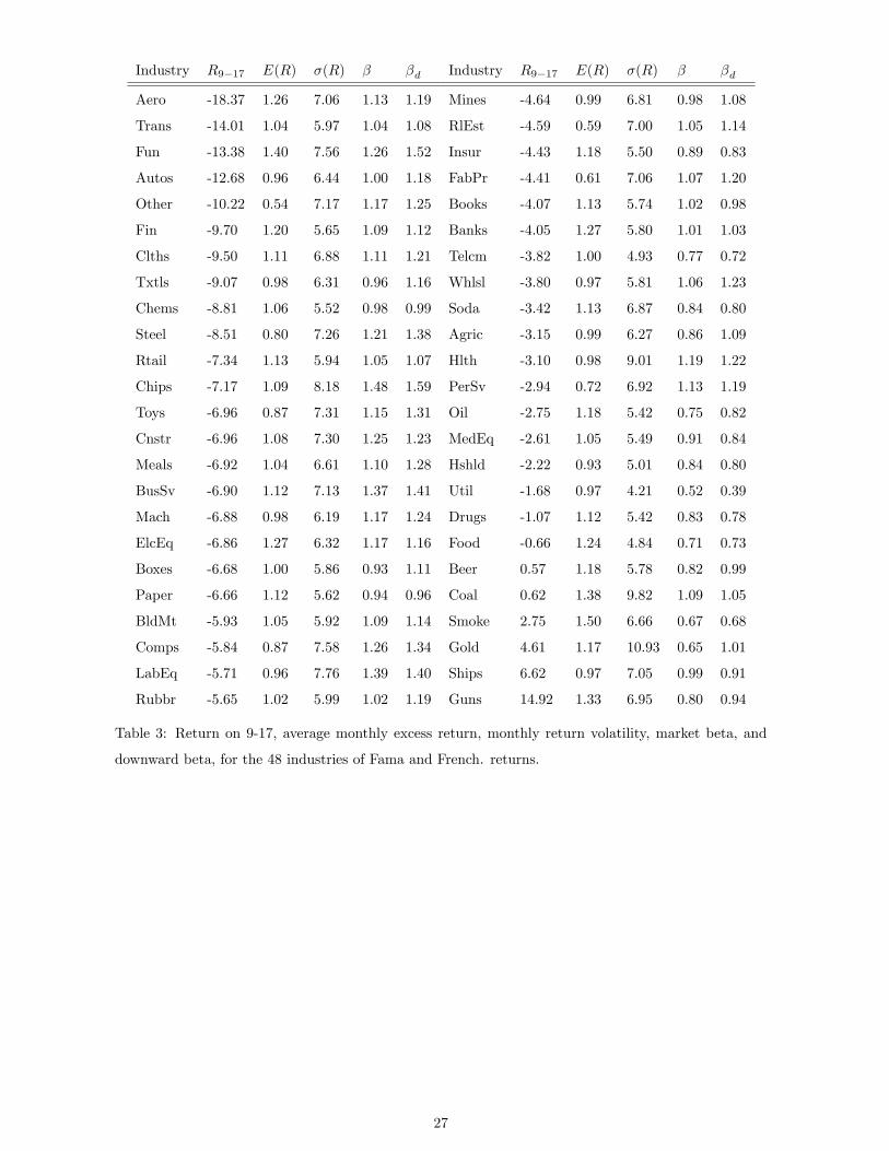
However, the correlation is slightly positive (0.20).19 Table 3 presents the 48 industries, sorted by their

return on 9/17, and the mean return, volatility of return, market beta, and disaster beta (to be de�ned

below).

17Barro (2006) also incorporates default of government bonds.18The 48 industry portfolios are taken from Prof. French�s website. These portfolios correspond roughly to two-digit

SIC industries. The mean excess return is calculated over the sample 1970-2004 using monthly data.19More formally, one could try and impose the formula (1) on this cross-section, but this does not work at all.

20

Figure 8 performs the same test for the 25 size and book-to-market sorted portfolios introduced

by Fama and French. In this case, the correlation is moderately negative (-0.16). Looking at the

other puzzles in the �nance literature, the Fama-French factor SMB was up 0.24%, HML was down

-0.93%, UMD was up 2.72%, and the small-value/small-growth excess return was -0.20%.20 Hence, only

HML and the small-value/small-growth excess return have the correct sign, and the magnitude is not

large. For instance, the value premium is roughly equal to the equity premium, so we would need value

stocks to do twice worse than growth stocks in disasters, i.e. we would require that HML was down by

approximately 10% on 9-11. This is ten times more than the data (-0.93%).

Of course one possible answer is that 9/11 is not the ideal experiment, and some stocks or industries,

such as aerospace may have been especially a¤ected by 9/11, more than they would be by another type

of disaster.

5.3 Measuring the Exposure to Large Downside Risk

The second test I perform is to compute the sensitivity of various portfolios of stocks to large declines

in the stock market more generally. Can the disaster explanation account for the cross-sectional puzzles

like value-growth, momentum, small-big which have attracted so much attention in the empirical �nance

literature?

Instead of taking the risk factor to be the market return, as in the CAPM, I pick the factor to

be the market return conditional on a large negative market return. Formally, I test the linear factor

model Mt = 1� bxt where xt =�Rmt+1 �R

ft+1

�� 1(Ri

t+1�Rft+1)<t

, where Rmt+1 is the market return and

Rft+1 is the risk-free return, and 1(:) is a characteristic function. I use monthly data and set arbitrarily

t = �10%. Since 1926 there have been 29 months where the excess market return is less than -10%.

This is equivalent to measuring the exposure of assets to large negative events by running the following

time series regression:

Rit+1 �Rft+1 = �i + �

di

�Rmt+1 �R

ft+1

�� 1(Ri

t+1�Rft+1)<t

+ "it+1; (4)

Securities which have a large �disaster beta��di do badly when the stock market does very badly. (This

can be justi�ed as an approximation to the model of section 2, since the market return in this case is

proportional to consumption growth.) I call this model the �Disaster CAPM�.

Following Cochrane (2001), I use GMM to estimate the factor model. For comparison, I also estimate

with the same procedure the CAPM. Table 4 presents the results, using three weighting matrix (the

identity matrix for the 1st stage, the optimal weighting matrix for the 2nd stage, and the Hansen-

Jagannathan recommended weighting matrix equal to the inverse of the covariance of returns). I use

three sets of test assets: the 6 Fama-French benchmark portfolios (intersection of 3 categories of size

and 2 categories of book-to-market), the 25 Fama-French size and book-to-market sorted portfolios, and

the 17 industry portfolios.21 Figure 9 presents the standard cross-sectional plots. This �gure makes

20SMB is a portfolio long small �rms and short large �rms; HML is long in �rms with high book-to-market and short

�rms in low book-to-market; UMD is long winners (�rms with high return in the past month) and short losers. All these

strategies generate signi�cant excess returns (see Table 4), which are not accounted for by CAPM or CCAPM betas.21Note that the 25 portfolios sample start only in July 1931, after the beginning of the Depression, due to missing data.

21

clear that the disaster model does not improve on the standard CAPM: the �t of the two models is very

similar. The statistics of Table 4 con�rm this: the J-statistic or the mean absolute pricing errors are

comparable across the two models, and are often worse for the disaster model.

The reason for the similarity of �t is simply that the disaster beta is highly correlated with the

market beta: for the 25 Fama-French portfolios, the correlation is over .96, and for the 17 industries

portfolios, it is over .95.

In Table 5, I perform the time-series regressions (4) for the excess returns HML, SMB, UMD and

small-value-small-growth. We see that the coe¢ cient �d does not explain very well the mean returns: for

UMD, it has the wrong sign, it is insigni�cant for SV-SG; for HML it is small and borderline signi�cant.

Only for SMB is there some empirical support for the disaster story: small �rms have indeed more

negative returns than large �rms when there is a big negative stock return.

The main problem with this section is that measuring the exposure to disasters is hard. However, the

preliminary conclusion is that there is little support in the data for disaster explanation when looking

at the cross-section of stock returns (value, momentum, industries), with the exception of size e¤ects.

[To be added: tests with consumption growth annual data during the Depression.]

Overall, there appears to be little support for this cross-sectional implication of the disaster model.

Of course, one may argue that the measures of exposure to disaster used in this note are highly imperfect.

It would be valuable to learn more about the historical properties of asset returns during disasters in

other countries and in other periods.

6 Conclusions

The disaster explanation of asset prices is attractive on several grounds: there are reasonable calibrations

which generate a sizeable equity premium. Disasters can easily be embedded in standard macroeconomic

models. Moreover, the explanation is consistent with the empirical �nance literature which documents

deviations from log-normality. Inference about extreme events is hard, so it is possible that investors�

expectations do not equal an objective probability. But precisely because the disaster explanation is not

rejected on a �rst pass, we should be more demanding, and study if it is robust and if it can account

quantitatively for other asset pricing puzzles. The current paper points toward some areas which would

bene�t from further study.

This is why I also consider the 6 benchmark portfolios, for which data is available since 1926.

22

References

[1] Ang, Andrew, Joe Chen and Yuhang Xing, 2006: �Downside Risk�, Review of Financial Studies,

19:1191-1239.

[2] Attanasio Orazio and Guglielmo Weber, 1989: �Intertemporal Substitution, Risk Aversion and the

Euler equation for Consumption�, Economic Journal 99: 5-73.

[3] Bansal Ravi and Amir Yaron, 2004: �Risks for the Long Run: A Potential Explanation of Asset

Pricing Puzzles�, Journal of Finance, 59: 1481-1509.

[4] Barro Robert, 2006: �Rare Disasters and Asset Markets in the Twentieth Century�, Quarterly

Journal of Economics 121:823-866.

[5] Barro, Robert, and Jose Ursua, 2008: �Consumption Disasters in the 20th Century�. Mimeo,

Harvard.

[6] Campbell, John, 1996. �Understanding Risk and Return�, Journal of Political Economy, 104(2):298-

345.

[7] Campbell, John, and John Cochrane, 1999: � By Force of Habit: A Consumption-Based Explana-

tion of Aggregate Stock Market Behavior�, Journal of Political Economy, 107(2):205�251.

[8] Campbell, John, 1999: �Asset Prices, Consumption, and the Business Cycle�, Chapter 19 in John

B. Taylor and Michael Woodford eds., Handbook of Macroeconomics, Volume 1, North-Holland:

Amsterdam, 1231-1303.

[9] Cerra, Valerie and Saxena Sweta. 2007: �The myth of economic recovery�. Forthcoming, American

Economic Review.

[10] Cochrane John, 2001: �Asset Pricing�, Princeton University Press

[11] Cochane John, 2007: �The Dog that did not Bark�, Review of Financial Studies, forthcoming.

[12] Epstein, Larry and Stanley Zin, 1989: �Substitution, Risk Aversion, and the temporal Behavior of

consumption and asset returns: A theoretical framework�, Econometrica 57: 937-969.

[13] Fama, Eugene and Kenneth French, 1996: �Multifactor Explanations of Asset Pricing Anomalies�.

Journal of Finance, 51(1):55-84.

[14] Fama, Eugene and Kenneth French, 1997: �Industry costs of equity�. Journal of Financial Eco-

nomics, 43:2, 153-193.

[15] Gabaix, Xavier. 2007. �Variable Rare Disasters: An Exactly Solved Framework for Ten Puzzles in

Macro-Finance�. Mimeo, NYU.

[16] Gabaix, Xavier, 2007b: �Linearity-Generating Processes: A Modelling Tool Yielding Closed Forms

for Asset Prices�. Mimeo NYU.

23

[17] Guvenen, Fathi, 2006: �Reconciling Con�icting Evidence on the Elasticity of Intertemporal Sub-

stitution: A Macroeconomic Perspective�, Journal of Monetary Economics 53: 1451-1472.

[18] Hansen, Lars and Kenneth Singleton, 1982: �Generalized instrumental variables estimation of

nonlinear rational expectations models�, Econometrica 50:1269-1286.

[19] Hall, Robert, 1988: �Intertemporal Substitution in Consumption�, Journal of Political Economy

96: 339-357.

[20] Holli�eld, Burt, Bryan Routledge and Stanley Zin, 2004: �Disappointment Aversion and the Cross-

Section of Returns�. Mimeo, CMU.

[21] Liu, Jun, Jun Pan and Tan Wang, 2005: �An Equilibrium Model of Rare-Event Premia and Its

Implication for Option Smirks�, Review of Financial Studies: 18:131�164.

[22] Maddison, Angus, 2003: The World Economy: Historical Statistics, Paris: OECD, 2003.

[23] Martin, Ian, 2007: �Consumption-Based Asset Pricing with Higher Cumulants�, Mimeo, Harvard.

[24] Mehra, Rajnish and Edward Prescott. 1985: �The Equity Premium: a Puzzle�. Journal of Monetary

Economics, 15:145-161.

[25] Mulligan Casey, 2004: �Capital, Interest and Aggregate Intertemporal Substitution�, Mimeo, Uni-

versity of Chicago.

[26] Polkovnichenko, Valery, 2006: �Downside Consumption Risk and Expected Returns�. Mimeo, U

Texas - Dallas.

[27] Ranciere, Romain, Aaron Tornell and Frank Westermann 2007: �Systemic Crises and Growth�,

Quarterly Journal of Economics, forthcoming.

[28] Rietz Thomas, 1988: �The Equity Premium: a Solution�, Journal of Monetary Economics 22:

117-131.

[29] Rodriguez, Carlos, 2006: �Consumption, the persistence of shocks, and asset price volatility�,

Journal of Monetary Economics, 53(8): 1741-1760.

[30] Stokey, Lucas and Prescott (1989). Recursive Methods in Economics Dynamics. Harvard University

Press.

[31] Vissing-Jorgensen Annette, 2002: �Limited Asset Market Participation and the Elasticity of In-

tertemporal Substitution�2002.�, Journal of Political Economy 110: 825:853.

24

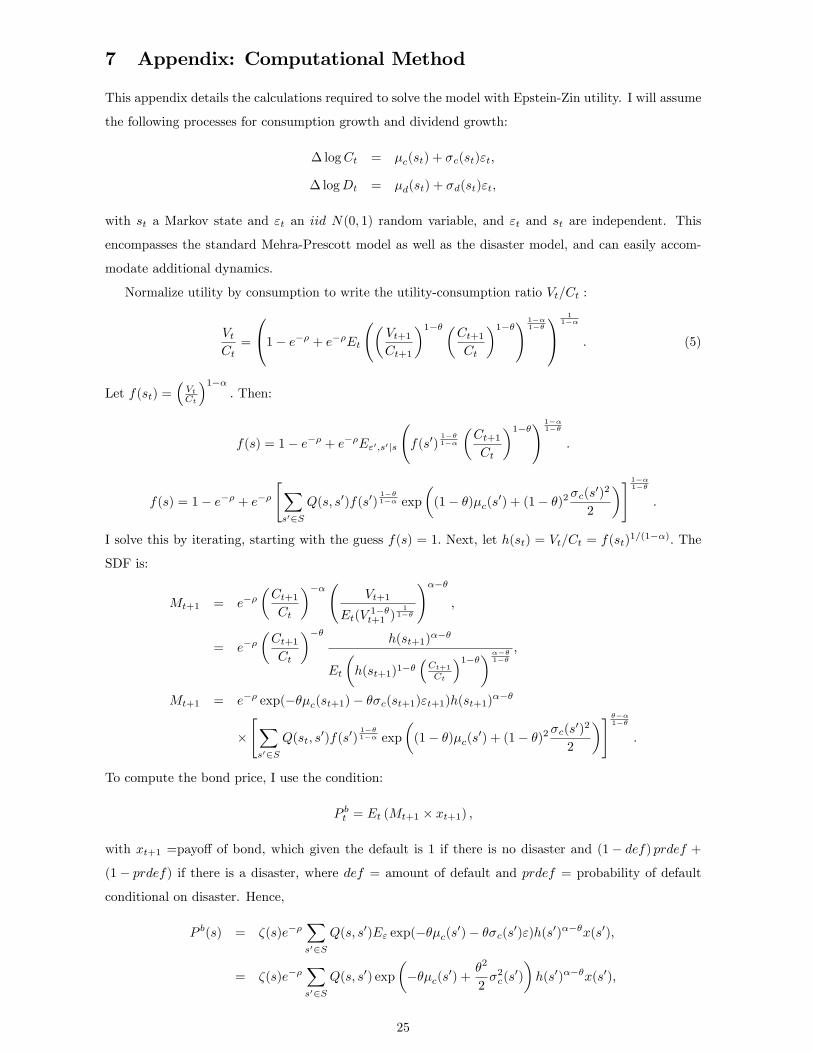
7 Appendix: Computational Method

This appendix details the calculations required to solve the model with Epstein-Zin utility. I will assume

the following processes for consumption growth and dividend growth:

� logCt = �c(st) + �c(st)"t;

� logDt = �d(st) + �d(st)"t;

with st a Markov state and "t an iid N(0; 1) random variable, and "t and st are independent. This

encompasses the standard Mehra-Prescott model as well as the disaster model, and can easily accom-

modate additional dynamics.

Normalize utility by consumption to write the utility-consumption ratio Vt=Ct :

VtCt=

0@1� e�� + e��Et � Vt+1Ct+1

�1�� �Ct+1Ct

�1��! 1��1��1A

11��

: (5)

Let f(st) =�VtCt

�1��: Then:

f(s) = 1� e�� + e��E"0;s0js

f(s0)

1��1��

�Ct+1Ct

�1��! 1��1��

:

f(s) = 1� e�� + e��"Xs02S

Q(s; s0)f(s0)1��1�� exp

�(1� �)�c(s0) + (1� �)2

�c(s0)2

2

�# 1��1��

:

I solve this by iterating, starting with the guess f(s) = 1: Next, let h(st) = Vt=Ct = f(st)1=(1��): The

SDF is:

Mt+1 = e���Ct+1Ct

��� Vt+1

Et(V1��t+1 )

11��

!���;

= e���Ct+1Ct

���h(st+1)

���

Et

�h(st+1)1��

�Ct+1Ct

�1������1��

;

Mt+1 = e�� exp(���c(st+1)� ��c(st+1)"t+1)h(st+1)���

�"Xs02S

Q(st; s0)f(s0)

1��1�� exp

�(1� �)�c(s0) + (1� �)2

�c(s0)2

2

�# ���1��

:

To compute the bond price, I use the condition:

P bt = Et (Mt+1 � xt+1) ;

with xt+1 =payo¤ of bond, which given the default is 1 if there is no disaster and (1� def) prdef +

(1� prdef) if there is a disaster, where def = amount of default and prdef = probability of default

conditional on disaster. Hence,

P b(s) = �(s)e��Xs02S

Q(s; s0)E" exp(���c(s0)� ��c(s0)")h(s0)���x(s0);

= �(s)e��Xs02S

Q(s; s0) exp

����c(s0) +

�2

2�2c(s

0)

�h(s0)���x(s0);

25

�(s) =

"Xs02S

Q(s; s0)f(s0)1��1�� exp

�(1� �)�c(s0) + (1� �)2

�c(s0)2

2

�# ���1��

:

The realized bond return is xt+1=P bt = x(st+1)=Pb(st); the expected bond return conditional on the

current state is cbr(s) = Et (xt+1) =Pb(st) =

Ps02S Q(st; s

0)x(s0)=P b(st); and the unconditional bond

return is E�Et (xt+1) =P

b(st)�=P

s2S �(s)cbr(s) where � is the ergodic distribution of the markov

chain fstg :

Finally, I calculate the value of equity with the standard recursion:

PtDt

= Et

�Mt+1

�1 +

Pt+1Dt+1

�Dt+1Dt

�;

which shows that PtDtis a function of the state variable st : PtCt = g(st): I again �nd g by iterating on

this recursion:

g(st) = Et

0BBB@e���Ct+1Ct

��� �Dt+1Dt

�0BBB@ h(st+1)

Et

�h(st+1)1��

�Ct+1Ct

�1��� 11��

1CCCA���

: (g(st+1) + 1)

1CCCA ;

g(s) = e���(s)Xs02S

Q(s; s0) exp

��d(s

0)� ��c(s0) +(�d(s

0)� ��c(s0))22

�h(s0)��� (g(s0) + 1) :

The conditional equity return is then:

ecr(s) =E"0;s0js

�(g(s0) + 1) Dt+1

Dt

�g(s)

=

Ps02S Q(s; s

0) (g(s0) + 1) exp(�d(s0) + �d(s

0)2=2)

g(s);

and the unconditional equity return is simplyP

s2S �(s)ecr(s):

26

Industry R9�17 E(R) �(R) � �d

Aero -18.37 1.26 7.06 1.13 1.19

Trans -14.01 1.04 5.97 1.04 1.08

Fun -13.38 1.40 7.56 1.26 1.52

Autos -12.68 0.96 6.44 1.00 1.18

Other -10.22 0.54 7.17 1.17 1.25

Fin -9.70 1.20 5.65 1.09 1.12

Clths -9.50 1.11 6.88 1.11 1.21

Txtls -9.07 0.98 6.31 0.96 1.16

Chems -8.81 1.06 5.52 0.98 0.99

Steel -8.51 0.80 7.26 1.21 1.38

Rtail -7.34 1.13 5.94 1.05 1.07

Chips -7.17 1.09 8.18 1.48 1.59

Toys -6.96 0.87 7.31 1.15 1.31

Cnstr -6.96 1.08 7.30 1.25 1.23

Meals -6.92 1.04 6.61 1.10 1.28

BusSv -6.90 1.12 7.13 1.37 1.41

Mach -6.88 0.98 6.19 1.17 1.24

ElcEq -6.86 1.27 6.32 1.17 1.16

Boxes -6.68 1.00 5.86 0.93 1.11

Paper -6.66 1.12 5.62 0.94 0.96

BldMt -5.93 1.05 5.92 1.09 1.14

Comps -5.84 0.87 7.58 1.26 1.34

LabEq -5.71 0.96 7.76 1.39 1.40

Rubbr -5.65 1.02 5.99 1.02 1.19

Industry R9�17 E(R) �(R) � �d

Mines -4.64 0.99 6.81 0.98 1.08

RlEst -4.59 0.59 7.00 1.05 1.14

Insur -4.43 1.18 5.50 0.89 0.83

FabPr -4.41 0.61 7.06 1.07 1.20

Books -4.07 1.13 5.74 1.02 0.98

Banks -4.05 1.27 5.80 1.01 1.03

Telcm -3.82 1.00 4.93 0.77 0.72

Whlsl -3.80 0.97 5.81 1.06 1.23

Soda -3.42 1.13 6.87 0.84 0.80

Agric -3.15 0.99 6.27 0.86 1.09

Hlth -3.10 0.98 9.01 1.19 1.22

PerSv -2.94 0.72 6.92 1.13 1.19

Oil -2.75 1.18 5.42 0.75 0.82

MedEq -2.61 1.05 5.49 0.91 0.84

Hshld -2.22 0.93 5.01 0.84 0.80

Util -1.68 0.97 4.21 0.52 0.39

Drugs -1.07 1.12 5.42 0.83 0.78

Food -0.66 1.24 4.84 0.71 0.73

Beer 0.57 1.18 5.78 0.82 0.99

Coal 0.62 1.38 9.82 1.09 1.05

Smoke 2.75 1.50 6.66 0.67 0.68

Gold 4.61 1.17 10.93 0.65 1.01

Ships 6.62 0.97 7.05 0.99 0.91

Guns 14.92 1.33 6.95 0.80 0.94

Table 3: Return on 9-17, average monthly excess return, monthly return volatility, market beta, and

downward beta, for the 48 industries of Fama and French. returns.

27

E (R) E(RjRm < �:1) E(RjRm < �:15) �d

HML 0.40 -0.68 0.15 0.08

t-stat 3.47 -0.53 0.09 1.90

SMB 0.24 -2.69 -2.68 0.18

t-stat 2.19 -3.63 -1.90 4.59

UMD 0.76 4.26 5.97 -0.24

t-stat 5.01 3.24 2.56 4.23

SV-SG 0.49 0.48 0.46 0.02

t-stat 4.14 0.41 0.33 0.41

Table 4: Mean returns on the HML, SMB, UMD and small growth-small value portfolios, for the full

sample, the sample of market declines greater than ten percent or �fteen percent, and the disaster beta.

­15 ­10 ­5 0 5 10

0.1

0.2

0.3

0.4

0.5

0.6

0.7

0.8

0.9

1

Agric

 Food

Soda

Beer

Smoke

T oys

Fun

 Books

Hshld

Clths

Hlth

MedEq

Drugs

Chems

Rubbr

T xtls

BldMtCnstr

Steel

FabPr

Mach

ElcEq

Autos

Aero

Ships

Guns

Gold

 Mines

Coal

 Oil

Uti l T elcm

PerSv

BusSv

Comps

Chips

LabEq

Paper

BoxesT rans

Whls l

Rtail

Meals

Banks

Insur

RlEs t

Fin

Other

return on sept 17, 2001

mea

n m

ont

hly 

exc

ess

 ret

urn

 197

0­2

004

Figure 7: Mean monthly excess return (1970-2004) and return on 9-17-01, for 48 portfolios of stocks

sorted by industry. Data from prof. French�s website.

28

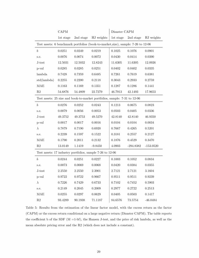
CAPM Disaster CAPM

1st stage 2nd stage HJ weights 1st stage 2nd stage HJ weights

Test assets: 6 benchmark portfolios (book-to-market,size), sample: 7-26 to 12-06

b 0.0251 0.0249 0.0219 0.1025 0.1076 0.0901

s.e. 0.0076 0.0074 0.0072 0.0430 0.0414 0.0390

J-test 12.5031 12.5032 12.8243 11.6305 11.6305 12.0926

p-val 0.0285 0.0285 0.0251 0.0402 0.0402 0.0335

lambda 0.7428 0.7359 0.6485 0.7261 0.7619 0.6381

std(lambda) 0.2255 0.2200 0.2118 0.3043 0.2933 0.2759

MAE 0.1163 0.1169 0.1351 0.1287 0.1286 0.1441

R2 54.6876 54.4809 22.7279 46.7913 42.1493 17.9653

Test assets: 25 size and book-to-market portfolios, sample: 7-31 to 12-06

b 0.0276 0.0252 0.0243 0.1213 0.0675 0.0823

s.e. 0.0079 0.0056 0.0053 0.0503 0.0405 0.0336

J-test 49.3752 49.3753 49.5270 42.8140 42.8140 46.9350

p-val 0.0017 0.0017 0.0016 0.0104 0.0104 0.0034

� 0.7879 0.7190 0.6920 0.7667 0.4265 0.5201

s.e. 0.2239 0.1597 0.1522 0.3181 0.2557 0.2127

MAE 0.1790 0.2011 0.2132 0.1876 0.4529 0.3470

R2 13.0149 1.1419 -9.8450 4.0903 -294.8382 -153.0520

Test assets: 17 industry portfolios, sample 7-26 to 12-06

b 0.0244 0.0251 0.0227 0.1003 0.1052 0.0834

s.e. 0.0073 0.0069 0.0068 0.0420 0.0384 0.0355

J-test 2.2550 2.2550 2.3901 2.7121 2.7121 3.1604

p-val 0.9722 0.9722 0.9667 0.9511 0.9511 0.9239

� 0.7226 0.7429 0.6733 0.7102 0.7452 0.5903

s.e. 0.2149 0.2045 0.2009 0.2977 0.2722 0.2513

MAE 0.0255 0.0297 0.0629 0.0405 0.0503 0.1417

R2 93.4289 90.1938 71.1187 84.6576 73.5754 -46.0484

Table 5: Results from the estimation of the linear factor model, with the excess return as the factor

(CAPM) or the excess return conditional on a large negative return (Disaster CAPM). The table reports

the coe¢ cient b of the SDF (M =1-bf), the Hansen J-test, and the price of risk lambda, as well as the

mean absolute pricing error and the R2 (which does not include a constant).

29

­9 ­8 ­7 ­6 ­5 ­4 ­3 ­2­0.5

0

0.5

1

1.5

S1

S2

S3

S4

S5

MS1

MS2

MS3MS4

MS5

M1

M2M3

M4

M5

ML1

ML2

ML3ML4

ML5

L1L2

L3L4

L5

return on sept 17, 2001

mea

n m

onth

ly e

xce

ss re

turn

 197

0­20

04

Figure 8: Mean monthly excess return (1970-2004), and return on 9-17-01, for 25 portfolios of �rms

sorted by size and book-to-market. Data from prof. French�s website.

30

0 0.5 10

0.2

0.4

0.6

0.8

1

1.2

1.4

6 FF benchmark assets

0 0.5 10

0.2

0.4

0.6

0.8

1

1.2

1.4

data

 mea

n ex

cess

 ret

urn,

 % p

er m

onth

0 0.5 1 1.50

0.5

1

1.5

25 size­BM

0 0.5 1 1.50

0.5

1

1.5

predicted mean excess return, % per month

0 0.5 10

0.2

0.4

0.6

0.8

1

1.2

17 industry portfolios

0 0.5 10

0.2

0.4

0.6

0.8

1

1.2

Figure 9: Estimation of two single-factor model: the CAPM (top panel) and the Disaster CAPM (bpttom

panel). The test assets are (a) left column: the 6 benchmark portfolios of Fama and French (sorted by

size and book-to-market), sample July 1926 to December 2006; (b) center column: the 25 Fama-French

size and book-to-market sorted portfolios, sample July 1931 to December 2006; (c) right column: the

17 industry portfolios, sample July 2006 to December 2006. The �gure displays the GMM 1st stage

results. The factors are demeaned prior to estimation.

31

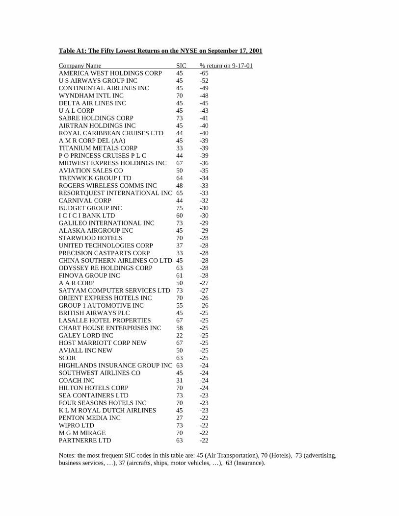
Table A1: The Fifty Lowest Returns on the NYSE on September 17, 2001 Company Name SIC % return on 9-17-01 AMERICA WEST HOLDINGS CORP 45 -65 U S AIRWAYS GROUP INC 45 -52 CONTINENTAL AIRLINES INC 45 -49 WYNDHAM INTL INC 70 -48 DELTA AIR LINES INC 45 -45 U A L CORP 45 -43 SABRE HOLDINGS CORP 73 -41 AIRTRAN HOLDINGS INC 45 -40 ROYAL CARIBBEAN CRUISES LTD 44 -40 A M R CORP DEL (AA) 45 -39 TITANIUM METALS CORP 33 -39 P O PRINCESS CRUISES P L C 44 -39 MIDWEST EXPRESS HOLDINGS INC 67 -36 AVIATION SALES CO 50 -35 TRENWICK GROUP LTD 64 -34 ROGERS WIRELESS COMMS INC 48 -33 RESORTQUEST INTERNATIONAL INC 65 -33 CARNIVAL CORP 44 -32 BUDGET GROUP INC 75 -30 I C I C I BANK LTD 60 -30 GALILEO INTERNATIONAL INC 73 -29 ALASKA AIRGROUP INC 45 -29 STARWOOD HOTELS 70 -28 UNITED TECHNOLOGIES CORP 37 -28 PRECISION CASTPARTS CORP 33 -28 CHINA SOUTHERN AIRLINES CO LTD 45 -28 ODYSSEY RE HOLDINGS CORP 63 -28 FINOVA GROUP INC 61 -28 A A R CORP 50 -27 SATYAM COMPUTER SERVICES LTD 73 -27 ORIENT EXPRESS HOTELS INC 70 -26 GROUP 1 AUTOMOTIVE INC 55 -26 BRITISH AIRWAYS PLC 45 -25 LASALLE HOTEL PROPERTIES 67 -25 CHART HOUSE ENTERPRISES INC 58 -25 GALEY LORD INC 22 -25 HOST MARRIOTT CORP NEW 67 -25 AVIALL INC NEW 50 -25 SCOR 63 -25 HIGHLANDS INSURANCE GROUP INC 63 -24 SOUTHWEST AIRLINES CO 45 -24 COACH INC 31 -24 HILTON HOTELS CORP 70 -24 SEA CONTAINERS LTD 73 -23 FOUR SEASONS HOTELS INC 70 -23 K L M ROYAL DUTCH AIRLINES 45 -23 PENTON MEDIA INC 27 -22 WIPRO LTD 73 -22 M G M MIRAGE 70 -22 PARTNERRE LTD 63 -22 Notes: the most frequent SIC codes in this table are: 45 (Air Transportation), 70 (Hotels), 73 (advertising, business services, …), 37 (aircrafts, ships, motor vehicles, …), 63 (Insurance).

Table A2: The Fifty Highest Returns on the NYSE on September 17, 2001 Company Name SIC % return on 9-17-01 COMDISCO INC 73 6.3 NELSON THOMAS INC 27 6.4 CARBO CERAMICS INC 32 6.4 JACOBS ENGINEERING GROUP INC 87 6.6 GOLDEN WEST FINANCIAL CORP 67 6.6 MACK CALI REALTY CORP 67 6.6 LORAL SPACE COMMUNICATIONS 48 7.1 HILB ROGAL HAMILTON CO 64 7.2 T V X GOLD INC 10 7.5 TRITON P C S HOLDINGS INC 48 7.8 VINTAGE PETROLEUM INC 13 7.9 BLACKROCK INC 62 7.9 FIRST AMERICAN CORP CALIF 63 7.9 GENCORP INC 30 8 C N O O C LTD 13 8.1 FEDERAL SIGNAL CORP 37 8.8 GENERAL DYNAMICS CORP 37 9.1 ORBITAL SCIENCES CORP 37 9.4 WILLIS GROUP HOLDINGS LIMITED 64 9.4 BROWN BROWN INC 64 9.7 MERIDIAN GOLD INC 10 9.7 HARRIS CORP 36 9.8 TELEFONICA MOVILES S A 48 10 CHINA MOBILE HONG KONG LTD 48 10 FLAGSTAR BANCORP INC 60 11 STURM RUGER CO INC 34 11 COMPANIA DE MINAS BV SA 10 11 NOKIA CORP 36 12 CAMPBELL RESOURCES INC NEW 10 13 U R S CORP NEW 87 14 TITAN CORP 36 14 LOCKHEED MARTIN CORP 37 15 TEFRON LTD 23 15 HECLA MINING CO 10 15 UNITED INDUSTRIAL CORP 87 15 GALLAGHER ARTHUR J CO 64 16 NORTHROP GRUMMAN CORP 37 16 COEUR D ALENE MINES CORP ID 10 16 TELEDYNE TECHNOLOGIES 87 18 GLAMIS GOLD LTD 10 18 U S AGGREGATES INC 14 19 WACKENHUT CORP 73 19 AMERICAN WATER WORKS INC 49 19 ALLIANT TECHSYSTEMS INC 36 21 EDO CORP 36 23 WACKENHUT CORP 73 27 RAYTHEON CO 38 27 BETHLEHEM STEEL CORP 33 28 DELTA WOODSIDE INDS INC NEW 50 29 L 3 COMMUNICATIONS HLDGS INC 36 38 ARMOR HOLDINGS INC 73 39