Disaster Mitigation Geotechnology 11 · 1.1 Soil particle density T m m m m w s a b s ... Standard...

Disaster Mitigation Geotechnology

11

Soft ground engineering

1 Physical tests

1.1 Soil particle density

Tmmm

mw

bas

ss

Picnometer

Soil particles m a

Distilled water

m b

Distilled water + soil particles

m s Soil particles

Distilled water

m a m b m s

ma, mb and ms do not include the mass of the picnometer.

1.2 Water content

ma mb mc

炉乾燥により蒸発

cb

ba

mm

mmw

×100 ＝ ×100

Evaporation by oven-drying

ma, mb and mc can include the mass of the plate.

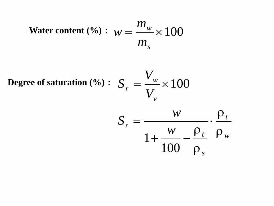
Water content (%)： 100s

w

m

mw

Degree of saturation (%)： 100v

w

rV

VS

w

t

s

t

r w

wS

1001

Enlarged photograph

of Sand

SEM image

of clay

r

s

w Sew

Physical Properties of soils

(low compressibility) sand < w, e < clay (high compressibility)

w=1.0g/cm3

s2.7g/cm3

Sr100%

Water content w vs.

Degree of saturation Sr

1.4 Liquid limit and plastic limit

Rock flour crashed by the glacial. SEM image of north European clay

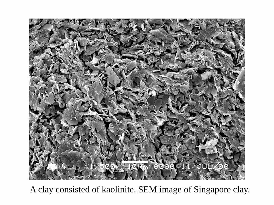
A clay consisted of kaolinite. SEM image of Singapore clay.

15mm

Liquid limit test

Is fall cone test used in Vietnam?

3mm でボロボロ

Plastic limit test

Collapse at 3mm in diameter

Plasticity index:

PLP wwI

c

P

(%)μm2thanfiner weightbyContents

indexPlasticity

F

IA

Activity:

0

20

40

60

80

100

120

0 40 80 120 160

液性限界 w L (% )

塑性指数

I

P

圧縮性：大

塑性：大

圧縮性：大

塑性：小

圧縮性：小

塑性：小

圧縮性：小

塑性：大

A線：I P =0.73(w L-20)

B線：w L=50

Qualitative evaluation of soil properties using a relationship

between plasticity index and liquid limit (=Plasticity chart)

Pla

stic

ity i

ndex

IP

Liquid limit wL (%)

B-line:

wL = 50

A-line:

IP = 0.73(wL – 20)

Compressibility: Small

Plasticity: Large Compressibility: Large

Plasticity: Large

Compressibility: Small

Plasticity: Small

Compressibility: Large

Plasticity: Small

w Lw p w n

0

5

10

15

20

0 40 80 120 160

含水比 w (% )

海底面からの深さ

(m

)

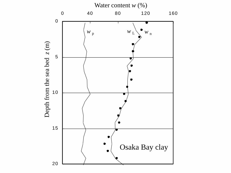
Osaka Bay clay

Water content w (%)

Dep

th f

rom

the

sea

bed

z

(m)

Question 1

A soil with a water content w of 100% collected from a

seabed is considered:

-How much is the liquid limit wL?

-Can you judge that this soil is sand, silt, or clay?

-How much is the void ratio e?

-How much is the effective unit weight g' ?

-How much is the overburden effective stress s'v0 at a

depth of 10 m from G.L.

How much is the compression index Cc?

Note that you can use the relation ship expressed as Cc = a ×(wL – b) with

a = 0.009 and b = 10 for e.g. European clays or

a = 0.0125 and b = 20 for e.g. Asian clays (Japanese clays), for example.

There are many proposals.

Question 2



-How much is the void ratio e? (Question 1)







Consolidation test

Methods for consolidation tests can be classifiedf into two types.

One type is called an incremental loading oedometer test (and

was commonly called a standard consolidation/oedometer test)

and the other is called a constant rate of strain loading

consolidation test.

Incremental loading consolidation (oedometer) test:

Standard specimens are 60 mm in diameter and 20 mm in

height, and are set in a metallic (e.g. stainless steel/brass)

consolidation ring with a high rigidity.

The consolidation tester (=oedometer) is set up, and loading

weights are prepared corresponding to the loading stages.

供試体重錘

供試体

(a) Before test (b) Load at the

third stage

Specimen Specimen loading

weight

供試体重錘

供試体

供試体

供試体

(a) Before test (b) Load at the

third stage

(d) Load at the

final stage (c) Load at the sixth stage

Specimen Specimen

Specimen Specimen

loading

weight

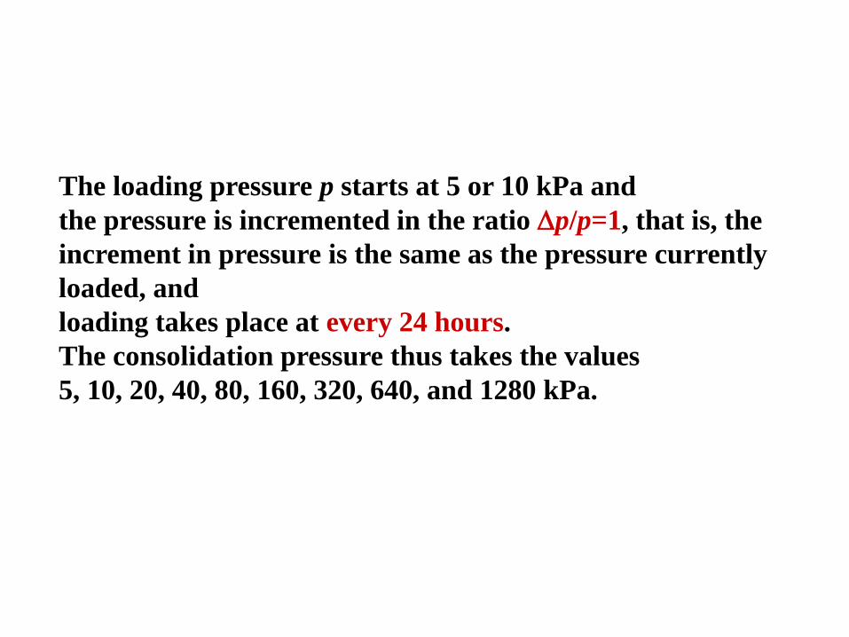
The loading pressure p starts at 5 or 10 kPa and

the pressure is incremented in the ratio Dp/p=1, that is, the

increment in pressure is the same as the pressure currently

loaded, and

loading takes place at every 24 hours.

The consolidation pressure thus takes the values

5, 10, 20, 40, 80, 160, 320, 640, and 1280 kPa.

The commonly employed consolidation test is the incremental

loading oedometer test in which the load is doubled each time.

However, in a “consolidation test at a constant rate of strain

(the CRS consolidation test),” the compressive strain is

produced at a constant rate. It is common to use an axial

strain rate of 0.01 to 0.02 %/min in testing.

The incremental loading oedometer test only yields data at

discrete points, but the CRS consolidation test has the

remarkable advantage of producing a continuous e – log p

relationship.

0.6

0.8

1.0

1.2

1.4

1.6

1.8

2.0

2.2

10 100 1000 10000

圧密圧力 s'v, p (kPa)

間隙比

e

CRS

段階載荷

pypy

0.6

0.8

1.0

1.2

1.4

1.6

1.8

2.0

2.2

10 100 1000 10000


間隙比

e

CRS

段階載荷

pypy

Consolidation pressure

Void

ratio

IL

py , pc , σ'p

It can be seen that most of the points measured by using

the incremental loading oedometer test, indicated by ,

almost agree with the results of the constant rate of

strain consolidation test.

However, the values for the consolidation yield stress py

are significantly different; the results of the constant rate

of strain (CRS) consolidation test, obtained from

continuous data,

give larger values.

0.6

0.8

1.0

1.2

1.4

1.6

1.8

2.0

2.2

10 100 1000 10000


間隙比

e

CRS

段階載荷

pypy

0.6

0.8

1.0

1.2

1.4

1.6

1.8

2.0

2.2

10 100 1000 10000


間隙比

e

CRS

段階載荷

pypy

Consolidation pressureConsolidation pressure

Void

ratio

Void

ratio

ILIL

When e – log p is calculated from the incremental loading

oedometer test data, one's attention is inevitably drawn to

the pressures for which data exists, and

the relationship cannot be correctly evaluated near the

consolidation yield stress py where there is a large

variation in curvature.

This is likely to be one reason that the value may be

miscalculated.

0.6

0.8

1.0

1.2

1.4

1.6

1.8

2.0

2.2

10 100 1000 10000


間隙比

e

CRS

段階載荷

pypy

0.6

0.8

1.0

1.2

1.4

1.6

1.8

2.0

2.2

10 100 1000 10000


間隙比

e

CRS

段階載荷

pypy

Consolidation pressureConsolidation pressure

Void

ratio

Void

ratio

ILIL

0

3

6

9

12

15

18

0 50 100 150 200

圧密降伏応力 p y (kPa)

深さ

z

(m

)

Consolidation yield stress py (kPa)

Depth

(m

)

Data from incremental

loading oedometer test (image)

Kansai Int. Airport

1000kPa

Dp/p

1.0 0.5 0.25

2000kPa

0

50

100

150

200

Ele

vation

z (

m)

0 1000 2000

pc, s'v0

s'v0

Dp/p

1.0 0.5 0.25

s'ys'v0

( 250)

( 200)

( 150)

( 100)

( 50)

0

0 1500 3000

Yield stress s'y (kPa)

0

50

100

150

200

Ele

vation

z (

m)

0 1000 2000 3000

pc, s'v0

s'v0

Incremental

loading

Constant strain rate

CRS -71m

K0 -72m

K0 -40m

K0 -98m

CRS -76m

CRS -101m

CRS -130m

CRS -158m

CRS -208m

0.4

0.6

0.8

1.0

1.2

1.4

1.6

1.8

2.0

2.2

10 100 1000 10000

Consolidation pressure s'v (kPa)

Vo

id r

atio

e

e – log p curves

obtained from CRS

consolidation test

wLwp wn

- 250

- 200

- 150

- 100

- 50

0

0 60 120

Water content w (%)

siltclay<5m

sand

( 250)

( 200)

( 150)

( 100)

( 50)

0

0 50 100

Fraction (%)

s'ys'v0

( 250)

( 200)

( 150)

( 100)

( 50)

0

0 1500 3000

Yield stress s'y (kPa)

- 250

- 200

- 150

- 100

- 50

0

1.0 1.5 2.0

OCR

-250

-200

-150

-100

-50

0E

leva

tio

n z

(m

)

H. clay

P. clay

P. clay

P. clay

P. clay

sand

sand

P. clay

P. clay

P. clay

Coefficient of

consolidation cv

cm2/day cm2/min cm2/s

m2/day m2/min

m2/s

1 6.94E-4 1.16E-5 1E-4 6.94E-8 1.16E-9

10 6.94E-3 1.16E-4 1E-3 6.94E-7 1.16E-8

100 6.94E-2 1.16E-3 1E-2 6.94E-6 1.16E-7

1000 6.94E-1 1.16E-2 1E-1 6.94E-5 1.16E-6

1.44 0.001 1.67E-5 1.44E-4 1E-7 1.67E-7

14.4 0.01 1.67E-4 1.44E-3 1E-6 1.67E-6

144 0.1 1.67E-3 1.44E-2 1E-5 1.67E-5

1440 1 1.67E-2 1.44E-1 1E-4 1.67E-4

Question 3

How much longer consolidation period is required for

a clay layer in 18-m thickness than a clay layer in 9-m

thickness? (note that these 2 layers have the same

consolidation characteristics)

How much longer consolidation period is required for

a clay layer with a coefficient of consolidation cv of 10

cm2/day than a clay layer with a cv of 100 cm2/day.

Explain an influence of loading stages on the

consolidation yield stress py obtained in the

incremental loading consolidation test.

Question 4

There is a 10-m thick marine clay deposit with a water

content w of 100% under the sea.

The water depth at this site is 2 m. If 4-m thick sand is

filled on this clay layer, how much settlement is

expected?

How long consolidation period is approximately

estimated up to 90%-degree of consolidation in 2

cases with a relatively larger cv value and relatively

smaller cv value?

Shear strength

In-situ test

Standard Penetration Test =SPT (N-value)

Cone Penetration Test = CPTU (qt, ud, fd)

Laboratory test

Undisturbed Sample Sampling Method

In Japan,

“sampling + laboratory tests” is for clayey soils

“SPT” is for sandy soils

Sampling

How to collect an undisturbed sample

Thin-walled tube sampler with fixed piston

For soft clay, Japanese standard

Role of piston is important

Denison sampler (Rotary double tube sampler)

For stiff clay

A scene of boring investigation.

Steel platform Spud barge

(S.E.P.)

Large-scale steel

platform and tower

100 m

eter

s lo

ng,

typic

ally

Rod coupling

Sampler head

Ball cone clamp Spider Adapter

Screw to attach the

sampling tube

Sampling tube

Inside diameter;

750.5 mm

External diameter

Venting bolt

Packing set screw

Packing Piston base

Piston rod

Chain

Turnbuckle

Swivel

Piston rod

Piston

Piston rod

Ball cone clamp

Spider

Adapter

Drain hole

Piston

Spring

Spring

Thin-walled tube sampler

with fixed piston

10

00

mm

×

○

Cone cramp

(a) (b) (c) (d)(a) (b) (c) (d)Sampling procedure using the Japanese thin-walled tube

sampler with fixed piston

Boring derrick is placed on the stage by crane.

Photos of boring survey in Japan

An old scene to assemble the boring derrick.

Anything can be assembled with scaffolding timbers and annealing wires.

A scene of boring investigation.

The clearance between the working deck and ground can provide an effective work.

Thin walled tube sampler with fixed piston.

(back: extension rod type, front: hydraulic operation type)

Thin walled tube sampler with

fixed piston:

Left: hydraulic operation type

Right: extension rod type

Thin walled tube sampler with fixed

piston (Hydraulic operation type).

Completely extended state. An o-ring

can be seen in the drainage holes.

Setting scene of the hydraulic operation type sampler.

The sampler is held by rod holder.

Sampler is efficiently lowered

by using rod tong.

in other countries

In case of extension rod type sampler, the inner rods must be connected.

Adjusting the level of sampler using the rod tong.

The assistant hands over the boring rod

from the derrick. The boring rods are rested against the

derrick.

The inner rod is fixed to the derrick

through the chain. Penetration length of

80 cm is marked by chalk on the boring

rod.

The sampler is penetrated into the bottom of bore hole in a fixed condition of the piston.

After the penetration, sampler was first

jacked up slowly.

The inner rod is removed

before detaching boring rod.

The sampler is lifted up.

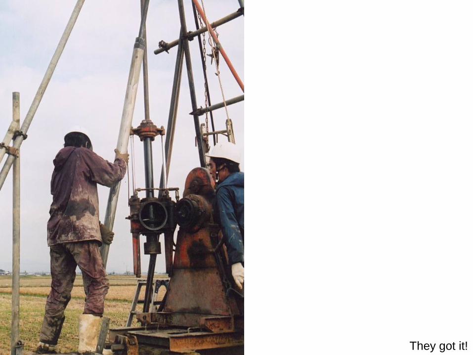
They got it!

Disturbance in the sampling

Stress release Inevitable

Mechanical disturbance

(Strain, Deformation, Crack)

Depends on the Sampling method

-Remolding type・・・Shallow and Soft clay

-Crack type・・・Deep and Stiff clay

Stress path

during the

sampling

A: Ideal sample

Impossible by

stress release

B: Perfect sample

No mechanical

disturbance

with stress release

Disturbance Ratio

R = s'p/s's 3—6

A: Ideal

P: Perfect

G: UU-test

F: UC-test

Boring

Sampling

Extruding

Trimming

Horizontal stress

Ver

tica

l st

ress

Disturbance ratio and Strength reduction

Range of R

Strength anisotropy

Difference between

Compressive and Extensive strengths

Inherent anisotropy by deposition

Induced anisotropy by stress anisotropy

(isotropic stress, K0-value)

10m 10m

Micro-structure of clay (SEM images)

Singapore clay Pusan clay

Pyrite: FeS2

Diatom: SiO2

Abundant Kaolin

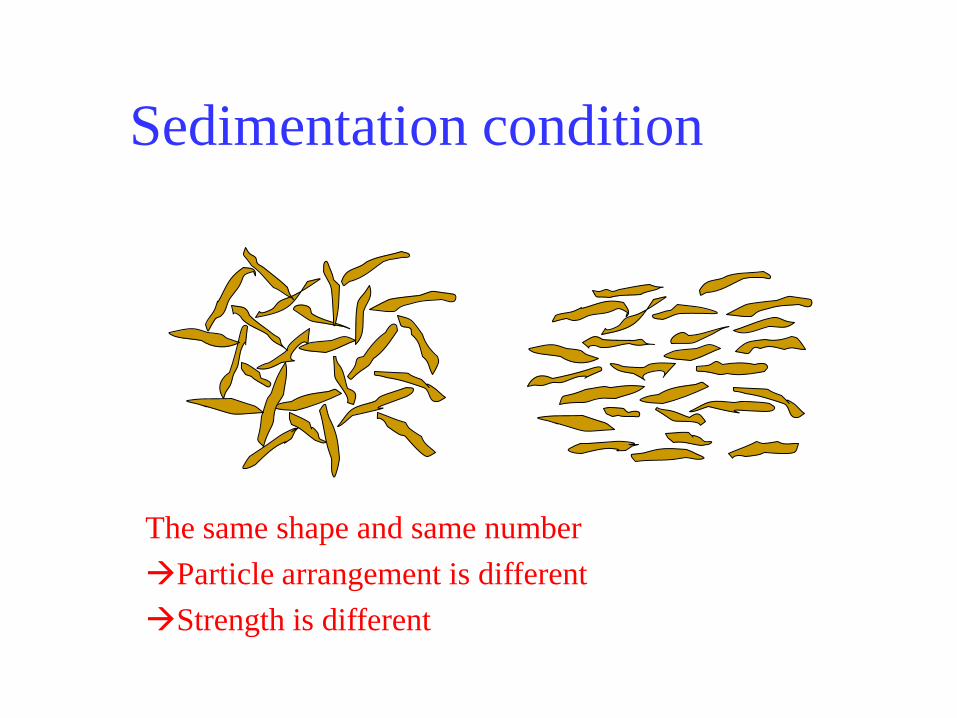
Sedimentation condition

The same shape and same number

Particle arrangement is different

Strength is different

Anisotropy on shearing direction

su＝(suc+2sus+sue)／4

su=(suc+sue)／2 or su=sus

Strength anisotropy sue/suc≒0.7

Triaxial

Extension

sue

Triaxial

Compression

suc

Direct

Shear

sus

56m

56m

83m

83m

193m

193m

142m

142m

-1400

-700

0

700

1400

0 700

Effective mean stress

p' (kPa)

De

via

tor

str

ess

q (

kP

a)

(b)

56m

56m

83m

83m

193m

193m

142m

142m

-1400

-700

0

700

1400

0 4 8 12

Axial stress e (%)

De

via

tor

str

ess

q (

kP

a)

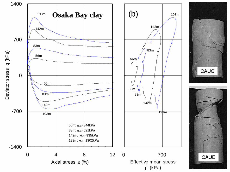
56m: s'v0=344kPa

83m: s'v0=521kPa

142m: s'v0=935kPa

193m: s'v0=1302kPa

(a)

Osaka Bay clay

Prerequisite for UC test Sampling by thin-walled tube sampler with fixed

piston moderate disturbance (= slight disturbance)

Followings cause “too much disturbance”

Sampling in slipshod manner

Using poor sampler

Shock during the transportation

Careless trimming

Shock into the specimen

Smaller strength is obtained Over design

Strain rate effect

Actual failure

UC，UU 0.88

Strain rate

Str

ength

rat

io a

gai

nst

s u a

t st

rain

rat

e of

1.0

%/m

in

Shear strength for design

su* = (qu/2) x c1 x c2 x c3

c1: correction factor for sample disturbance

c2: correction factor for strength anisotropy

c3: correction factor for strain rate

c1 = 1.0(perfect sample)／0.7(average disturbance)

c2 = ｛1.0(compression) +0.7(extension)｝／2 = 0.85

c3 = 0.85(e=1.0%／min and 0.01%／min)

c1 x c2 x c3 ≒ 1 ［Lucky Harmony］

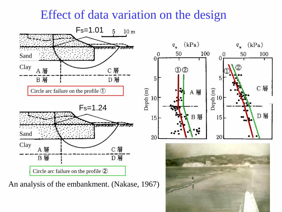
Effect of data variation on the design

An analysis of the embankment. (Nakase, 1967)

Fs=1.24

Fs=1.01

Circle arc failure on the profile ①

Circle arc failure on the profile ②

Dep

th (

m)

Dep

th (

m)

Clay

Sand

Clay

Sand

Application of UC strength based on the experience

An application for a failure of Japanese clay

Be careful for other marine clays with different characteristics (disturbance, anisotropy, strain rate effect)

#Stability analysis by using UC strength

Common sense in Japan, but

NOT Common in other countries

UU-test valid for crack type disturbance

CU-test (Consolidation with s'v0) valid for remolding type disturbance

To obtain a reliable test result …

Recompression method

Minimize the effect of disturbance

s'v0

s'v0

K0s'v0 s'h0=K0s'v0

s'v0

s'v0

K0s'v0 K0s'v0

In-situ Recompression

K0：Coefficient of earth

pressure at rest

Triaxial CU

compression and

Extension test

UC strength and

Triaxial compressive &

extensive strengths

10

30

50

70

0 50 100 150 200

非排水せん断強度 s u (kPa) 深さ

z (

m)

●： s uc

○： s ue

×： q u /2

Undrained shear strength c u (kN/m 2 )

c uc

c ue

Dep

th

z (

m)

The undrained shear strength (qu/2) obtained from UC test varies much, but the average value agrees with the mean value of the triaxial compressive and extensive strengths with recompression method.

Why the Triaxial test does not

become popular ?

Because it is costly (=expensive) !

The cost of Isotropic Consolidated Undrained

Compression Triaxial test (CIU-test) is more

than 10 times of UC test.

Anisotropic consolidation with recompression

method is more expensive

K0-consolidation is much more expensive

Practical application of Triaxial test is still

difficult today even in Japan!

Question 1

A soil with a water content w of 100% collected from a seabed is

considered:

-How much is the liquid limit wL?

In the shallow seabed, wL=wn then wL100%

-Can you judge that this soil is sand, silt, or clay?

clay


Using eSr = (s/w)w with s=2.7g/cm3, then e=2.7 (s/w=Gs)

-How much is the effective unit weight g' ?

g’= (s-w)g/(1+e)=(2.7-1.0)×9.8/(1+2.7)=4.5kN/m3

-How much is the overburden effective stress s'v0 at a depth of 10 m

from G.L.

s’v0=g’×z=4.5×10=45kN/m2

How much is the compression index Cc?

For Asian clays (Japanese clays)

Cc 0.0125×(wL – 20) is known as empirical equation, thus,

Cc 0.0125×(100 – 20) = 1.0

Question 2


considered:

-How much is the void ratio e? (Question 1)

Using eSr = (s/w)w with s=2.7g/cm3, then e=2.7


considered:




considered:



Question 3

How much longer consolidation period is required for a clay layer in 18-

m thickness than a clay layer in 9-m thickness? (note that these 2 layers

have the same consolidation characteristics)

Since required consolidation time is proportional to H2 (the law of

squared H), if thickness is twice, required consolidation time is 4 times.

How much longer consolidation period is required for a clay layer with a

coefficient of consolidation cv of 10 cm2/day than a clay layer with a cv

of 100 cm2/day.

Required consolidation time is proportional to 1/cv, if cv is 1/10 times,

required consolidation time becomes 10 times.

Explain an influence of loading stages on the consolidation yield stress

pc obtained in the incremental loading consolidation test.

Because compression curve obtained from incremental loading

oedometer test tends to yield at an existing data point, the consolidation

yield stress pc tends to be underestimated, in particular for a structured

clay by ageing effect. In order to solve this problem, it is useful that

either incremental loading ratio is decreased around pc in order to

obtain dense data set around pc or compression curve obtained

constant rate of strain consolidation test is used as a curve ruler in

order to fit the data set obtained from incremental loading oedometer

test.

Question 4

There is a 10-m thick marine clay deposit with a water content w of 100%

under the sea.

The water depth at this site is 2 m. If 4-m thick sand is filled on this clay

layer, how much settlement is expected?

wn=100 corresponds to e=2.7.

wL wn is empirically known for shallow depth seabed soil, and

using an empirical equation Cc = 0.0125×(wL – 20) for Japanese marine

clays, then Cc 1.0

g' = (s – w)g/(1+e) = (2.7 – 1.0)×9.8/(1+2.7) = 4.5kN/m3

At the middle depth of clay layer (z = 5m)

s'v0 = g ×z = 4.5×5 = 22.5kN/m2

Thus, effective unit weight of sand is g' = 9.8 kN/m3 (1kgf/cm3), and

above the water level, gt = 17.6kN/m3 (1.8kgf/cm3)

Incremental loading by filling is Dp = 2×9.8 + 2×17.6 = 54.8kN/m2

Therefore, consolidation settlement S can be estimated by the following

equation:

S = Cc×H / (1 + e)×log{(s' v0 + Dp) / s'v0}

=1.0×10 / (1 + 2.7)×log{(22.5 + 54.8) / 22.5} = 1.4m

Question 4 (cont’d)

How long consolidation period is approximately estimated up to 90%-

degree of consolidation in 2 cases with a relatively larger cv value and

relatively smaller cv value?

Approximately cv=10cm2/day in a case of slow consolidation, and

cv=100cm2/day in a case of rapid consolidation. When clay thickness is

10 m with double side drainage, maximum drainage distance H* is 5 m

(= 500 cm), and then

In a case of slow consolidation:

t90 = H*2/cv×Tv90 = 500×500 / 10×0.848 = 21200 day 58 year

In a case of rapid consolidation:

t90 = H*2/cv×Tv90 = 500×500 / 100×0.848 = 2120 day 5.8 year

where time factor at 90% degree of consolidation is Tv90 = 0.848.

In order to obtain the coefficient of consolidation cv, consolidation test

is strongly required.

Disaster Mitigation Geotechnology 11 · 1.1 Soil particle density T m m m m w s a b s ... Standard...

Documents

Transcript of Disaster Mitigation Geotechnology 11 · 1.1 Soil particle density T m m m m w s a b s ... Standard...