Sede Amministrativa: Università degli Studi di Padova

Dipartimento di Economia e Management “Marco Fanno”

Scuola di dottorato di ricerca in : Economia e Management

Ciclo: XXV

Econometrics of vice:

Idle students, partisan prosecutors and environmental predators.

Direttore della Scuola : Ch.mo Prof. Giorgio Brunello

Supervisore : Ch.mo Prof. Giorgio Brunello

Dottorando : Pablo Torija

1/113

2/113

PH.D. THESIS

Econometrics of vice:

Idle students, partisan prosecutors and

environmental predators.

Pablo Enrique Torija Jiménez.

University of Padova.

Supervisor:

Giorgio Brunello

3/113

4/113

To Karin and Emilito

5/113

6/113

Laß dir nichts einreden,

Sieh selber nach!

Was du nicht selber weißt,

Weißt du nicht.

Prüfe die Rechnung,

Du mußt sie bezahlen.

Bertolt Brecht

7/113

8/113

TABLE OF CONTENTS:

Page

Introduction (English) 11

Introduzione (Italiano) 15

Chapter 1. Straightening PISA: When students do not want to

answer standardized tests. 19

Chapter 2. Stories on corruption: How media and prosecutors

influence elections. 51

Chapter 3. Responding to the Climate Change Challenge:

Experimental Evidence 67

Acknowledgements 113

9/113

10/113

INTRODUCTION

(English)

This thesis is organized in three clearly differentiated chapters. The three of them

deal with currently relevant issues: The effect of low-quality of standardized tests on

research, the high levels of political corruption in Spain and the collective capacity of

tackle climate change.

In the first chapter “Straightening PISA: When Students do not Want to

Answer Standardized Tests”, I study one of the key elements on current education

policies: The standardized-tests. Concretely, I analyze how students approach standardized

tests in different ways. I use a measure of effort exerted by students belonging to different

countries and social groups in order to assess the impact of low effort on the student's final

score. The measure links an acknowledged psychological tests (Dot-Counting test) with one

PISA-item, in which students had to merely count dots. In this chapter, I measure to

which extent different effort levels may distort the score of students. This problem would

affect social-science research when standardized-tests are use. At the end of the chapter, I

propose a simple solution to design standard tests which would eliminate this problem.

Given the importance of standardized-tests on the design of education programs, this

paper may be a contribution to implement more accurate education policies.

The second chapter focuses on one key issue of Spanish current political crisis: The

level of political corruption. Political institutions developed during the Spanish transition

to democracy are currently criticized due to their inability to stop political corruption. For

instance, Spanish Attorney Generals are appointed by the government and their

impartiality is usually criticized. In “Stories on Corruption: How Media and

Prosecutors Influence Elections”, I analyze systematically the partiality of the last

11/113

two Attorney Generals. Concretely, I study whether Attorney Generals try to influence

elections by adjusting the tempo of their investigations to the electoral calendar. This

possibility is combined with the mass media editorial decisions. I analyze whether mass

media have a partisan bias and hide corruption activities of their preferred parties. For

doing so, I have created a unique database: I have coded the number of articles containing

the word “corruption” of the two main Spanish newspapers “El Pais” and “El Mundo”

every week in the last ten years. After the econometric analysis I found significant evidence

of the partisan behavior of both the Attorney Generals and mass media.

The last chapter is a joint work with Karolina Safarzynska from the

Wirtschaftsuniversität Wien.

“Responding to the Climate Change Challenge: Experimental Evidence”

tackles the problem of climate change and the capacity of societies to overcome it. This

chapter has also a different methodology. Precisely, it is based on experimental methods.

We consider isolated groups of individuals which must extract resources form a

renewable common-pool. The novelty is the study of the impact of resource uncertainty on

individual harvests in common-pool resource dilemmas together with the possibility of

group collapse. The uncertainty is modeled as a weather shock diminishing the groups'

resources, which is drawn from the distribution known in advance to participants. On the

other hand, the group collapses if the resources go below a certain threshold. In that case

all accumulated resource-extraction get lost. This can be interpreted as the minimum

harvests below which a group does not have sufficient nutrition to survive.

We find that in the long run, sufficiently severe weather shocks can induce

individuals to conserve resources. However, in the short-run uncertainty leads to resources

over-exploitation. In addition, our results suggest that resource uncertainty undermines

effectiveness of costly sanctioning. In some treatments, individuals can punish others at

their own cost. We found that the possibility to punish others induce individuals to harvest

significantly more resources in the beginning of the experiment, compared to the situation

12/113

when sanctioning is not possible. The presence of punishment paradoxically increases the

probability of resource exhaustion. We interpret these results in the context of the World

climate change. We conclude that the positive impact of environmental pressure on

individual behavior and the effect of new institutions are likely to come too late to prevent

damage to the environment.

13/113

14/113

INTRODUZIONE

(Italiano)

Questa tesi è organizzata in tre capitoli chiaramente differenziati. I tre capitoli

riguardano argomenti attualmente rilevanti: l’effetto della bassa qualità dei test

standardizzati in ricerca, gli alti livelli di corruzione politica in Spagna e la capacità

collettiva di rispondere ai cambiamenti climatici.

Nel primo capitolo “Rafforzando PISA: quando gli studenti non vogliono fare i test

standardizzati”, studio uno degli elementi chiave nelle attuali politiche per l’educazione: i

test standardizzati. Concretamente, analizzo come gli studenti affrontano i test

standardizzati in modi differenti. Uso una misura di sforzo fatto degli studenti che

appartengono a Paesi diversi e gruppi sociali diversi per stimare l’impatto del basso sforzo

nel punteggio finale degli studenti. La misura collega un test psicologico molto affermato (il

test di conta dei punti) con una domanda del test PISA, nella quale gli studenti devono

semplicemente contare i punti. In questo capitolo, misuro fino a che punto diversi livelli di

sforzo fatto degli studenti possono distorcere il punteggio del PISA. Questo problema

avrebbe degli effetti sulla ricerca nelle scienze sociali, quando vengono utilizzati i risultati

dei test standardizzati. Alla fine del capitolo, propongo una semplice soluzione per il design

di test standardizzati che elimini questo problema. Data l’importanza dei test

standardizzati nel design dei programmi educativi, questo articolo potrebbe essere un

contributo per implementare politiche educative più accurate.

Il secondo capitolo si focalizza su uno dei temi chiave della attuale crisi politica

spagnola: il livello di corruzione. Le istituzioni politiche sviluppate durante la transizione

spagnola verso la democrazia sono attualmente sotto forte critica a causa della loro

15/113

incapacità nel fermare la corruzione politica. Per esempio, i procuratori generali spagnoli

sono nominati dal governo e la loro imparzialità è spesso criticata. Nel capitolo “Storie

sulla corruzione: come i media e I procuratori influenzano le elezioni”, analizzo

sistematicamente la parzialità degli ultimi due procuratori generali. Concretamente, studio

se i procuratori generali tentano di influenzare le elezioni modificando la tempistica delle

loro indagini adattandola al calendario elettorale. Questa possibilità è combinata con le

decisioni editoriali dei mass media. Analizzo se i mass media hanno un pregiudizio

ideologico e nascondono le storie di corruzione dei loro partiti preferiti. Per fare questo, ho

creato un database unico: ho codificato il numero di articoli contenenti la parola

“corruzione” nei due quotidiani principali spagnoli, “El Pais” e “El Mundo”, ogni

settimana negli ultimi dieci anni. Dopo un’analisi econometria ho scoperto una evidenza

significativa di un comportamento partigiano sia dei procuratori generali che dei mass

media.

L’ultimo capitolo è un lavoro congiunto con Karolina Safarzynska della

Wirtschaftsuniversität Wien.

“Rispondendo alla sfida del cambiamento climatico: evidenze sperimentali” affronta

il problema del cambiamento climatico e la capacità delle società di superarlo. Questo

capitolo usa una metodologia differente. Precisamente si basa su metodi sperimentali.

Noi consideriamo gruppi isolati di individui che devono estrarre risorse da un bacino di

risorse rinnovabili.

La novità è lo studio dell’impatto dell’incertezza di risorse sui raccolti individuali nei

dilemma dei bacini di risorse rinnovabili, unita alla possibilità che il gruppo collassi.

L’incertezza è modellata come uno shock atmosferico che diminuisce le risorse dei gruppi,

che è estratto da una distribuzione conosciuta in anticipo dai partecipanti. D’altro canto il

gruppo collassa se le risorse scendono sotto una certa soglia. In quel caso tutta l’estrazione

accumulata di risorse viene persa. Questo potrebbe essere interpretato come il minimo

raccolto sotto al quale il gruppo non ha nutrimento sufficiente per sopravvivere.

16/113

Scopriamo che nel lungo termine, shock atmosferici abbastanza severi possono

indurre gli individui a conservare le risorse. Comunque, nel breve termine l’incertezza porta

ad un sovrasfruttamento delle risorse. Inoltre, i nostri risultati suggeriscono che l’incertezza

nelle risorse danneggia l’effettività del sanzionamento costoso. In alcuni trattamenti, gli

individui possono punire altri pagando un costo. Scopriamo che la possibilità di punire

altri induce gli individui a raccogliere significativamente più risorse all’inizio

dell’esperimento, comparato alla situazione in cui il sanzionamento non è possibile. La

presenza della punizione paradossalmente incrementa la probabilità di un esaurimento delle

risorse. Interpretiamo questi risultati nel contesto del cambiamento climatico mondiale.

Concludiamo che l’impatto positivo della pressione climatica sul comportamento

individuale e l’effetto di nuove istituzioni probabilmente arrivano troppo tardi per

prevenire un danno all’ambiente.

17/113

18/113

Straightening PISA:

When Students do not Want to Answer Standardized Tests.

Abstract

In this paper I analyze how students approach standardized tests in different ways. I use a

measure of effort exerted by students belonging to different countries and social groups in

order to assess the impact of low effort on the student's final score. I demonstrate how this

can distort the results of researches who use standardized test databases (eg. those

provided by PISA). I propose a simple solution to design standard tests that eliminate this

problem.

19/113

1. Introduction

There is a large amount of money invested in international standardized tests which

try to measure the knowledge, skills and cognitive abilities of students from all around the

world. Periodically, media show the results of the last PISA test, and the position of the

own country is analyzed in depth by experts on education. Moreover, there is a growing

amount of national standardized tests looking for the performance of schools, regions and

provinces within countries.

All those studies are used in many scientific articles and institutional reports,

covering a wide spectrum of topics and perspectives. Some scholars use those tests to look

for links between economic growth, mortality, productivity or inequality and school quality,

using a macro-economic perspective (Hanushek and Kimko, 2000; Bosworth and Collins,

2003; Jamison, Jamison, and Hanushek 2006, Soto 2006, Altinok and Murseli 2007,

Hanushek and Woessmann, 2009, Barro and Lee 2010). Other scientists analyze the impact

of different school systems or the effectiveness of private schooling in the light of these test

results (Vandenberghe, 2003; Dronkers, 2008). In addition, there are single-country

analyses (Simola 2005, Sahlberg 2007, or Lokan, Geenwood, Cresswell 2008), and cross-

country comparisons (Kim, Lavonen and Ogawa 2009; Martin 2004). Finally, there is a

group of studies which analyze the knowledge acquired by certain sub-populations of

students. They compare mainly the test performance between immigrants and natives or

between female and male within and across countries (Creswell 2002; Ammermüller 2005;

OECD 2006; Schleicher 2006; White 2007). Consequently, all these reports build the basis

for national and international educational policies (e.g. Erlt 2006, Backes-Gellner and Veen

2008, Lundahl and Waldow, 2009, Lundgren 2010).

However, these tests are surrounded by an aura of skepticism. Some authors have

written a holistic critic about standardized tests, in which they are arguing that such tests

are unable to measure the main aspects of educational life (Rochex 2006, Sjøberg 2007).

Other researchers criticize more technical aspects of the tests. They point out the secrecy

20/113

of the items, (Rochex 2006 , Yus Ramos et al 2011), the limitation to pen and paper

problems (Sjøberg 2007) and the cultural differences across countries that may affect how a

question is understood or how a given topic is taught in class (McQueen and Mendelovits

2003, Rochex 2006, Fensham 2007). Furthermore, there is a large number of authors who

have criticized the translation of the items (Grisay, 2002, McQueen and Mendelovits 2003)

or the design of the items itself (Rochex 2006, Dohn 2007 , Yus Ramos et al 2011 and

Alcaraz Salarirche et al 2011).

One of the oldest critiques to this kind of tests is that they require total

collaboration of the surveyed students, who should exert a large effort on the test

(Borghans, et. Al 2007 , Sjøberg 2007). From a theoretical point of view, this view is

defended by several authors (eg. William 2008) and empirically, many have analyzed the

role of effort in standardized tests, specially in PISA and TIMSS. For instance, Baumert

and Demmrich (2001) conducted an experiment with different treatments in order to

increase the effort of test-takers. They found that it would be possible to increase the effort

of PISA-test-takers by giving financial rewards or feedback. Also Wise and DeMars (2011)

consider the possibility of student making “fast-guessing” decisions in the test. These

authors proposed a method to filter them.

This paper analyzes the importance of low motivation in the students' final test

score and quantifies its impact on PISA-test-takers. Furthermore, it looks for the

determinants of full cooperation, and it shows the potential bias cross-country and

individual-level studies, if the lack of collaboration of students is not considered.

Section 2 explains whether different students present different degrees of willingness

to answer (WTA). This will be followed by an analysis of how the WTA of students can be

measured by using certain PISA-test items. Then I will show the similarities between the

PISA-test items and psychological tests which measure low collaboration.

Section 3 presents a statistical summary of the econometric techniques used for the

analysis of the PISA database. It shows the approach used to find the potential bias in

21/113

individual-level and a cross-country studies.

Section 4 contains the main results of the paper. I carry out a round of regressions

where the endogenous variable is the PISA-test score. I analyze whether the coefficient of

selected explanatory variables changes if the WTA of the student is considered. I also

measure the total effect of the WTA on the student PISA-test score. The effects of a

measurement problem due to the differences on WTA across countries is also analyzed.

Section 5 summarizes the results and adds some recommendations. Concretely, the

results show how not considering the WTA of students leads, at best, to low t-values and,

in general, to biased results on the studies that use standardized tests. The end of this

section contains also a proposal to better quantify the WTA of students. This measure can

be implemented in the future in order to solve the problem analyzed.

2. Willingness to answer standardized tests.

The quality of the data gathered determines the quality of standardized tests. Good

data assumes, of course, that the respondents do their best to answer the questions of

standardized tests and that they are willing to concentrate on the test-items (Sjøberg

2007).

In order to study the effort of standard test takers, we can start by analyzing how a

standardized test takes place. According to the PISA-test administrator manual of 2000,

the PISA-test takes approximately three hours. The instructions are read for ten to fifteen

minutes. Then the students start to answer the cognitive test divided into two parts with a

braek in between from five to twenty minutes. Once the second part of the test is finished,

students receive a questionnaire in order to collect personal data (OECD 2000a). The time

for the test may be excessive (Sjøberg 2007), and even other similar tests such us TIMSS

require less time. For instance in the 2003 version, the TIMSS-test took 72 minutes for the

4th grade and 90 for the 8th grade (IEA 2003).

It is noteworthy that there is no economic reward for answering properly, that there

22/113

is no feedback on their own performance and no information about the right solutions is

distributed among the students. Sjøberg (2007) discusses that students of different

countries react very differently to such test situations due to their cultural environment

and to their attitudes towards school and education. He explains how a Taiwanese school

director, before a standardized test, gathered students and parents giving them a speech

about the significant task that they were facing. After that, and prior to the test, the

students marched while the national anthem was played (Sjøberg 2007).

The importance of the willingness to answer (WTA) in different tests is not a new

issue. More than forty years ago, scholars have already identified this problem (Borghans,

et. al 2007). Some empirical studies have shown how the reward through performance-

related prizes, both in cash or in candies, increases IQ test scores and the outcome of other

standardized tests (Schmeichel, Vohs, and Baumeister, 2003; and Pailing and Segalowitz

2004).

To overcome the problem of low WTA, psychologists have developed several

psychometric tools. These tools try to calibrate the level of effort or collaboration of test

takers. The four most used tests are the Rey 15-Item Test, the Dot Counting Test, the Rey

Word Recognition Test, and the B Test (Nitch and Gassmire 2007). The validity of these

tools relies on the floor-effect principle, which is that their demanded tasks are easy

enough for all individuals, even with neuropsychological deficits (Rogers, Harrell, and Liff,

1993).

I will concentrate on the Dot Counting test due to its similarities with an item of

the PISA-test. The standard version of the Dot Counting test consists on twelve cards with

varying numbers of dots which range from 7 to 28. Subjects are asked to count the dots

and verbalize their counts as fast as possible (Boone, Lu, and Herzberg, 2002). The fact

that counting is one of the earliest, most important number skills that children learn and

use (Nye, Fluck and Buckley, 2001), is the main reason for using dot counting as a valid

measure of effort and collaboration.

23/113

Studies which use this technique have shown that, even considering the forced stress

of the situation, normal individuals commit errors in only 10% of the trials (Beetar and

Williams 1995). A higher percentage of mistakes must be explained by a low effort exertion

(Beetar and Williams 1995).

The PISA-test presents a similar question to the Dot Counting test, namely the

question M136Q01T from PISA 2000 (see illustration 1). In this question students have to

count a certain number of points and crosses ranging from 1 to 32. The second part of the

question asks for further computations, namely guessing the number of dots which the

consecutive set of dots and crosses should have. Students receive points only if the second

part of the question is correctly answer. Fortunately, the database of PISA is coded in such

way that it shows whether the adolescents counted the dots correctly.

ILLUSTRATION 1

Samples of M136Q01T and Dot-Counting test

From the PISA-test, 35.2% of the students made a mistake when counting the dots.

Even though, students were not under time pressure; could keep the figures with the dots

in front of them, allowing for further re-counting, and were provided with pen an paper.

The number of registered mistakes is three times more than the Dot-Counting test

considers as normal for motivated individuals. All students are able to count as PISA-test

monitors are instructed not to give the test to those individuals mentally unable to do it

(OECD 2000a). Being this is the case, we should accept that there is a large amount of

exam takers who are not fully collaborative or who are not willing to answer.

Four the analysis, I henceforth consider that individuals are willing to answer the

24/113

test only if they counted correctly the points.

An important issue is that the number of correct answers is not equally divided

across countries. If the low percentage of correct answers came from aleatory mistakes,

then the percentage of mistakes should be the same in all the countries were PISA-test is

carried out. Graph 1 illustrates these differences.

GRAPH 1

Percentage of correct counting per country

Furthermore, the WTA does not vary only across countries, but it changes at

different points of time during the PISA-test. At the beginning, students may be more

keen to answer carefully but at the end the may be tired, bored, upset, or even, as

mentioned by the School quality monitor manual, “totally out of control” (OECD 2000a).

These factors influence the psychological condition of the student and therefore reduce

their motivation (Pajares 2007).

This is reflected in the percentage of number of students who count the dot

correctly when the dot-counting question is situated in different positions within the PISA-

test. Precisely, the percentage of right counts decreases when the question is situated later

25/113

JPNHKG

KORGBR

IRLNZL

NLDAUS

DNKCAN

CHEFIN

BELSWE

RUSUSA

CZEDEU

HUNESP

ISLAUT

FRANOR

POLITA

LUXLVA

PRTMEX

GRCBRA

0

0,1

0,2

0,3

0,4

0,5

0,6

0,7

0,8

0,9

1

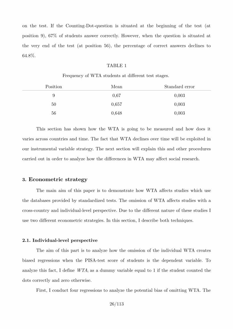
on the test. If the Counting-Dot-question is situated at the beginning of the test (at

position 9), 67% of students answer correctly. However, when the question is situated at

the very end of the test (at position 56), the percentage of correct answers declines to

64.8%.

TABLE 1

Frequency of WTA students at different test stages.

Position Mean Standard error

9 0,67 0,003

50 0,657 0,003

56 0,648 0,003

This section has shown how the WTA is going to be measured and how does it

varies across countries and time. The fact that WTA declines over time will be exploited in

our instrumental variable strategy. The next section will explain this and other procedures

carried out in order to analyze how the differences in WTA may affect social research.

3. Econometric strategy

The main aim of this paper is to demonstrate how WTA affects studies which use

the databases provided by standardized tests. The omission of WTA affects studies with a

cross-country and individual-level perspective. Due to the different nature of these studies I

use two different econometric strategies. In this section, I describe both techniques.

2.1. Individual-level perspective

The aim of this part is to analyze how the omission of the individual WTA creates

biased regressions when the PISA-test score of students is the dependent variable. To

analyze this fact, I define WTAi as a dummy variable equal to 1 if the student counted the

dots correctly and zero otherwise.

First, I conduct four regressions to analyze the potential bias of omitting WTA. The

26/113

first one considers only the PISA outcome and socioeconomic factors. The second one

includes also psychological aspects of the students. The third and fourth regressions

replicates the previous regressions (1 and 2) but incorporate WTAi.

These are the regressions expressed mathematically:

PISAi = α + β1 SEi + ei (1)

PISAi = α + β1 SEi + β2 PSi + ei (2)

PISAi = α + β1 SEi + β3 WTAi + ei (3)

PISAi = α + β1 SEi + β2 PSi + β3 WTAi + ei (4)

By comparing the vectors β1, it is possible to measure the existing bias of those

studies which use standardized tests at an individual-student level.

It can be argued, that there are other substantive variables not included in these

regressions which could be correlated with both WTAi and PISAi. Therefore, in order to

strength the validity of the coefficient β3, I conducted an instrumental variable (IV)

analysis.

Concretely, I exploit the fact that students answer mathematical questions in

different moments during the PISA test. Precisely, different students receive, randomly,

different set of questions, called booklets. In some booklets, students answer first the

mathematical part of PISA-test and later the reading and science parts. In these cases the

dot-counting question is at position 9.

In other booklets, students start with the reading and science exercises and answer

the mathematical part at the end. In those cases the dot-counting question is at position

50. As we have seen before, WTA declines over time meaning that those students

answering the mathematical questions at the beginning have provided a larger effort in the

mathematical part than those which answer the mathematical questions later on. This

difference helps us to avoid a weak instrument.

The formal econometric technique is the following: First, I create a dummy variable

(POS) equal to 0 if the mathematical questions were at the beginning (dot-counting in

27/113

position 9) and 1 if these questions were answered later in the test (dot-counting in

position 50). And I conduct instrumental variables:

PISAi = α + β1 SEi + β3IV WTAi + ei (IV 1)

Using POSi as an instrument for WTAi

WTAi = α + β1 SEi + β2 POS i +ui (IV 2)

As we will see, the coefficients of β3IV and β3 are statistically the same and therefore,

β3 is preferred. Due to this, all the computations related with the instrumental variables

can be looked up in appendices (Appendix 1).

Regarding the IV, please notice that I have decided not to use the questioner with

the psychological variables, because students of many countries have not answered them.

Consequently, this increases the number of observations. I have also eliminated the

observations when the question was in position 56 as many students did not manage to go

that far in the test. Including these observations could generate a selection bias. In order to

increase comparability, I have also eliminated this booklet form the OLS regressions.

Finally, we should take into account the possibility of a measurement error problem.

Precisely, the dot counting exercise in the PISA-test is not a perfect imitation of the Rey

Dot Counting test. Another measurement error could be that students might make

mistakes in spite of being motivated. The data set provided by PISA does not help us to

disentangle between these two sources of errors. If any of these factors is present, we would

obtain a downward estimation of the role of WTA.

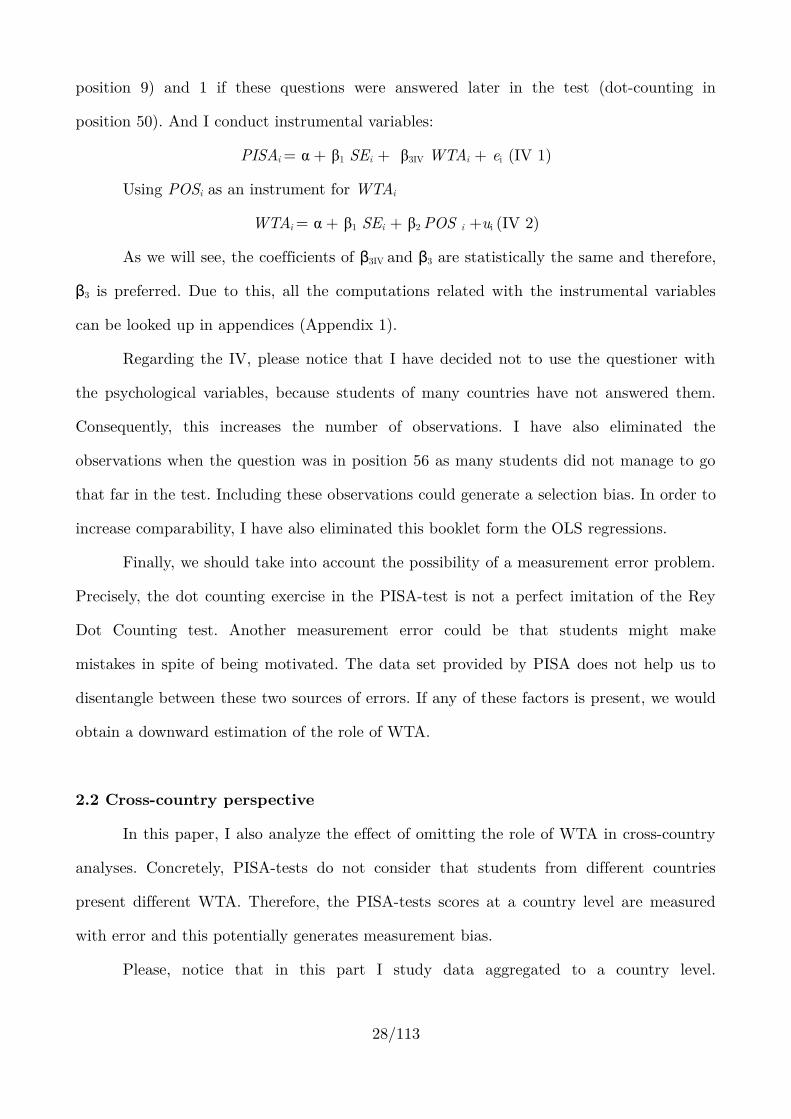
2.2 Cross-country perspective

In this paper, I also analyze the effect of omitting the role of WTA in cross-country

analyses. Concretely, PISA-tests do not consider that students from different countries

present different WTA. Therefore, the PISA-tests scores at a country level are measured

with error and this potentially generates measurement bias.

Please, notice that in this part I study data aggregated to a country level.

28/113

Therefore, WTAc is the percentage of students in a given country which counted correctly.

I will show whether WTA is correlated with the PISA-score at a country level. If

this is the case we have an non-classical measurement error which is more problematic

than the traditional measurement error. The regression is conducted as follows.

PISAc = α + β1 WTAc + ec (5)

Later, I will explain in detail the consequences of this problem. For doing so, I will

suppose that PISA is equal to the true quality of Education (Educc) plus an error term uc

PISAc = Educc + uc (6)

I will construct this error term relying in the theory which claims that PISA tests

and other standardized tests are a good measurement tool only when students are fully

motivated and cooperative (Sjøberg 2007; Borghans, Heckman, Lee and ter Weel 2007).

Educc should consider as motivated all the students of all countries. This is done by giving

to each country the extra points that every student would get if they where motivated -the

coefficient β3 from regression (4)- to every non motivated student:

u c=−β3(1−WTAc) (7)

Thanks to the estimation of this measurement error, I will be able to compute the

bias produced when PISA-test-score is used as a dependent variable in cross-country

regressions.

Finally, I will compare the differences between Educc and PISAc.

2.3 Further specifications:

In regressions (1) - (4) I use the PISA score as endogenous variable. There, I use the

student weights provided in the PISA-test database in order to obtain unbiased estimators.

Finally, I would like to clarify the statistical tools used for the regressions (1)-(4).

Concretely, PISA-test uses a technique called plausible numbers. Each student does not

receive one single grade but five different values which have to be taken into account when

performing an OLS regression. Because of that, I have modified the standard errorrs of the

29/113

coefficients of the regressions according to the instructions of OECD (2000b).

2.4 Variable description

I have included a number of socioeconomic variables to identify possible influences

on the PISA-test score and the level of motivation:

Private school ( priv ) : The variable priv is a dummy variable, equal to one if the

school attended by the student is private.

Economic status index ( eco ) : PISA index that combines the education of the parents

and their occupation at the time of the test being held. It is also correlated with time

preferences of the children and other non-cognitive variables (Heckman 2007).

Number of siblings ( nsib ) : The number of siblings affects the cognitive and non-

cognitive skills of students as parents must divide their effort in education among a larger

number of children (among others: Steelman, Powell, Werum and Carter 2002).

Language spoken at home ( langother ) : this variable is equal to one when the

language spoken at home is different from the official languages spoken in the country. A

low command of the language spoken may increase the relative difficulty of the exam for a

given student, increasing their fatigue and reducing her motivation (Pajares 2007).

Born abroad ( imm ): This variable is equal to one if the student is born in another

country. A student born abroad may not share the culture and the motivation of her

colleagues. It may also create special circumstances for the child's learning. (e.g. Bauer,

Lofstrom and Zimmermann 2000).

Female student ( female ): Gender factors may affect the motivation of the student.

Self-concept or interest in mathematics may differ across genders (e.g. Beaton et al., 1996).

This variable is equal to one for female students.

Country dummies: I have also included country dummies as intercepts of the

regression. Due to their number, country dummies are not shown in the tables.

In the next table I present a summary of these variables.

30/113

TABLE 2

Descriptive statistics (unweighted)

Observations Mean Standard Dev. Min Max

eco 32550 43.75 16.78 16 90

nsib 34220 1.86 1.32 0 12

langother 31638 0.05 0.22 0 1

priv 26455 0.19 0.39 0 1

imm 33209 0.07 0.25 0 1

female 34509 0.5 0.5 0 1Additionally, I have included the description of the psychological variables used in

the appendices (Appendix 2).

4. Results

This section presents the final analysis of the effect of WTA in the PISA-test. It is

divided into two parts. The first one includes the effects of omitting WTA when using

standardized tests at the individual-level, and the second one addresses the effect of

omitting WTA when standardized tests are used in a cross-country perspective.

3.1 Results at the individual-level

The first aim of the paper is to measure the consequences of omitting WTA, and to

measure the role of WTA in the individual PISA-test score.

The following table shows the coefficients of OLS regressions on PISA-test score

which include: Only socioeconomic factors (1), socioeconomic and psychological factors (2),

and the previous models and WTAi (3 and 4). I have also included the first and second

stages of the instrumental variable in order to compare the coefficient of WTA obtained

with OLS and the one obtained with IV methods (5 and 6). As I have mentioned before, a

detailed IV analysis con be found in the appendices (Appendix 1).

31/113

TABLE 3

Comparison of coefficients when considering WTA or not

Dependent variable: PISA-score Instrumental variables

1 2 3 4 5 1st -stage

62nd -stage

WTA 73.70 ***1.58

63.36 ***1.67

121.44 ***33.81

eco 1,33***0.04

1.22 ***0.04

1.08 ***0.04

0.94 ***0.04

0.003 *** 0.0002

0.89 ***0.12

nsib -7.65 ***0.58

-6.80 ***0.59

-6.08 ***0.052

-5.62 ***0.54

-0.02*** 0.003

-5.01 ***0.84

langother -36.18 ***3.94

-39.07 ***4.27

-34.61 ***3.61

-36.21 ***3.99

-0.037 * 0.021

-33.87 ***3.74

priv 18.44 ***2.28

13.08 ***2.27

13.65 ***2.12

9.71***2.14

0.07 *** 0.01

10.71 ***3.16

imm -21.87 ***3.03

-19.10 ***3.15

-17.68 ***2.76

-16.41 ***2.90

-0.06 *** 0.016

-14.02 ***3.30

female 12.80 ***1.33

7.59 ***1.29

13.76 ***1.23

9.60 ***1.32

-0.01 0.007

14.34 ***1.23

POS -0.03*** 0.007

constant 427.72 ***6.72

478.86 ***7.11

397.49 ***3.18

433.82 ***5.95

0.59*** 0.03

370.58 ***3.74

Psycho. variables?

NO YES NO YES NO NO

Number obs 18667 16071 18667 16071 18667 18667

R2 0.36 0.44 0.48 0.52 0.11 0.42Note: 1,2,3,4 Entries are plausible numbers coefficients with adjusted standard deviations below. R2 for OLS

regression. IV Entries are the coefficients for the IV strategy with robust standard deviations below. *** p< .

01; ** p < .05; * p <0.1. for two-tailed tests.

The first observation is that WTA is significant in both models (OLS and IV).

However a Hausman test indicates our preference for OLS models:

32/113

TABLE 4

Hausman test for endogenous regressors.

Endogeneity test of

endogenous regressors l2.16

Chi-sq(1) P-val 0.14

In general, the inclusion of WTA produces an increase in R2. Concretely, the

increase of variance explained from models 1 and 2 to models 3 and 4 is 12% and 8%

respectively. However, as I have mentioned before, this value can be a downward

estimation bias of the real impact of WTA. This is the first result of the paper:

Result 1: The willingness to answer accounts for at least for 8% to 12% of the total

variance of the PISA-test score.

As we can observe in column 5, many of the variables usually considered in

individual-level studies are correlated with WTA. This creates an omitted-variable

problem. If we exclude WTA from our regressions, the coefficients of the socioeconomic

variables change significantly. However, these changes vary from one variable to another.

The next table summarizes these changes.

33/113

TABLE 5

Percent change of the effect of socio-economic variables after using WTA

Variation without psycho. variables

Variation with psycho. variables

eco -23.1% -29.8%

nsib -25.8% -21.0%

langother -4.5% -7.9%

priv -35.1% -34.7%

imm -23.7% -16.4%

female 7.0% 20.9%

From a statistical perspective, whether the school is public or private is the variable

which experiences the largest variation. The influence of the private schooling in PISA-test

score declines if the WTA is considered. The effect of private schooling on learning is a hot

topic in education and labor studies (e.g. Vandenberghe, 2003; Dronkers, 2008). Further

research on the topic should take the fact into account that students coming from private

schools present significantly higher WTA.

Additionally, the differences in gender should be mentioned. Sulkunen (2007) claims

on this topic that PISA-test items are more interesting for girls that for boys (Sulkunen

2007). Moreover, if standardized tests are seen as a contribution to a public good (see

appendix 3), we should take into account that female students are usually more willing to

cooperate on such circumstances (e.g. Cadsby and Maynes 1998). Sulkunen (2007) suggests

that these problems, which are reflected also in our results, could be removed by changing

the items.

Finally, we cannot exclude that other individual or school characteristics are

affected by the omission of WTA. This could generate important research problems.

Together, all these effects represent the second main result of this paper.

34/113

Result 2: Results from PISA-tests studies which omit WTA are likely to be biased

due to the correlations between different socioeconomic variables and the WTA.

3.2. Cross-country perspective

So far I have analyzed the consequences of using these tests at an individual-level.

Now I analyze the problems which arise when researchers use those tests at a cross-country

level, with aggregated data.

First, I analyze whether the source of measurement error, WTA, is correlated with

the PISA-score at a country level.

TABLE 6

Regression of PISAc test on WTAc

Dependent variable: PISA

1

WTAc 225.89 ***(33.93)

Constant 329.46***(22.33)

R2 0.65

Number of Obs 32

Note: Entries are OLS coefficients with t-values in parentheses. *** p < .01; ** p < .05; * p < .10 for two-tailed tests.

The previous table shows the strong correlation between willingness to answer and

the PISA-test score. This provokes a non-classical measurement error (Fuller 1987). In

theory, non-classical measurement error can lead to an attenuation bias and it can even

reverse the sign of the effect of PISA if the measurement error is large (Fuller 1987). This

is the third result of the paper:

35/113

Result 3. The existence of measurement error problem creates an attenuation bias

when the standardized tests scores are used in a cross-country analysis.

It is possible to measure the level of attenuation biased produced when WTA is

omitted. Let's suppose that we want to analyze the impact of education quality (x) on a

given variable y :

y = βx + e (8)

But, we only have data on:

z = x + u (9)

Where z is the PISA-test score. Therefore, if E(u) = 0 and σ2xu ≠ 0, then the OLS-

estimator for β:

β=cov (x+u ,βx+e )

var (x+u)(10)

so that we have in this case:

plim β=β(σx

2+σxu)

σ x2+σu

2+2σxu

=(1−b uz )β (11)

where buz is the regression coefficient of a regression of u on z (Fuller 1987). In our

case, z is the PISA-test score and I have estimated u according to (7). Therefore, I can

calculate buz :

TABLE 7

Regression of uc on PISAc test

Dependent variable: uc

1

PISAc 0.16 ***(0.02)

Constant -78.41***(10.44)

R2 0.66

Number of Obs 32

Note: Entries are OLS coefficients with t-values in parentheses. *** p < .01; ** p < .05; * p < .10 for two-tailed tests.

36/113

According to this regression, we might conclude that the attenuation bias is around

16% when we use PISA-test score as a measurement of education quality.

Before presenting the conclusions, I include the new index (EDUC) showing the

position of the countries if WTA is considered. I normalize PISA and EDUC by giving the

value of 1 to the country with the largest score. I also include how many positions a given

country gains or looses with the new index.

37/113

TABLE 8Comparison PISA and EDUC

From the previous table, we can observe two main consequences of considering

WTA. First, there are several changes in the relative position of countries. Great Britain

and the Netherlands would be the countries which would lose the most positions if WTA is

taken into account, and Czech Republic the country which would gain the most. The

second consequence is that the differences in the educative systems across countries

diminish. The quality of educational systems seems to be much more similar when WTA is

considered.

38/113

PISA EDUC VariationHKG 1 HKG 1 0JPN 0,99 JPN 0,99 0KOR 0,98 KOR 0,98 0NZL 0,96 FIN 0,98 +1FIN 0,96 CZE 0,97 +3AUS 0,95 CAN 0,96 +1CAN 0,95 NZL 0,96 -3CZE 0,94 AUS 0,96 -2GBR 0,94 FRA 0,96 +2BEL 0,93 AUT 0,95 +2FRA 0,92 BEL 0,95 -1AUT 0,92 GBR 0,95 -4DNK 0,92 ISL 0,95 +1ISL 0,92 SWE 0,93 +1

SWE 0,91 NOR 0,93 +2IRL 0,9 DNK 0,93 -3NOR 0,89 CHE 0,91 +1CHE 0,89 USA 0,9 +1USA 0,88 IRL 0,9 -3DEU 0,88 DEU 0,9 0HUN 0,87 HUN 0,9 0RUS 0,85 POL 0,88 +2ESP 0,85 ESP 0,88 0POL 0,84 RUS 0,88 -2LVA 0,83 LVA 0,87 0NLD 0,82 ITA 0,86 +1ITA 0,82 PRT 0,86 +1PRT 0,81 GRC 0,85 +1GRC 0,8 LUX 0,84 +1LUX 0,8 NLD 0,83 -4MEX 0,69 MEX 0,74 0BRA 0,6 BRA 0,67 0

5. Conclusions

In this paper I have shown how some students may not be fully motivated during

standardized tests. I have analyzed this problem in depth, and I identify three main

results:

The willingness to answer of students accounts for the 8% - 12% of the PISA-test

variation.

Results obtained from using the PISA-test databases at the individual level are

likely to be biased if WTA is omitted.

Researches which consider the PISA-test databases at an a cross-country

perspective face a non-classical measurement if WTA is omitted.

Previous researches on education have used standardized tests assuming full

cooperation by the subjects. Therefore, we must be concerned with the validity of their

results, their conclusions and the proposals which emanate from their results.

I am aware of the differences between a pure motivation test, concretely the Dot-

Counting test, and the item M136Q01T from the PISA test. The results presented in this

paper do need to be taken with care but may still be used as a starting point for a better

use and design of standardized tests. For instance, it would be important to notice that

links between the socioeconomic variables and WTA are likely to vary across countries. For

instance, “Do girls and boys have a more similar WTA in Sweden than in Brazil?”, “How

do migrants from different countries approach these tests?”, etc.

In general, the problems previously mentioned and the limitations of this paper

could be avoided by introducing questions able to measure adequately the WTA of

students at different stages of standardized tests. Whether the used technique is the Dot-

Counting task or any other is a decision which must be made by expert psychologists.

However it is a relative cheap and easy to implement measure which could improve the

quality and exactness of social research

39/113

REFERENCES

Alcaraz Salarirche et al 2011 ¿Evalúa PISA la competencia lectora?, Revista de

Educación, 360. Enero-abril 2013 Forthcoming

Altinok, Nadir and Murseli, Hatidje, 2007. "International database on human capital

quality," Economics Letters, Elsevier, vol. 96(2), pages 237-244, August.

Ammermüller, A. (2005). 'Educational opportunities and the role of institutions',

ZEW Discussion Paper, No. 05-44.

Backes-Gellner, U. and Veen, S. (2008). The consequences of central exams on

educational quality standards and labour market outcomes. Oxford Review of Education,

43(5):569-588.

Bauer, P., Lofstrom, M., and K.F. Zimmermann (2000), “Immigration Policy,

Assimilation of Immigrants and Natives' Sentiments towards Immigrants: Evidence from 12

OECD-Countries”, Swedish Economic Policy Review, 7, 11-53.

Baumert, J., & Demmrich, A. (2001). Test motivation in the assessment of student

skills: The effects of incentives on motivation and performance. European Journal of

Psychology of Education, 16(3), 441-462.

Beaton, A. E., Martin, M. O., Mullis, I. V., Gonzales, E. J., Smith, T. A., & Kelly,

D. L. (1996). Science achievement in the middle school years: IEA's Third International

Mathematics and Science Study (TIMSS). Chestnut Hill, MA: Center for the Study of

Testing, Evaluation, and Educational Policy, Boston College.

Beetar, J. T., & Williams, J. M. (1995). Malingering response styles on the Memory

Assessment Scales and symptom validity tests. Archives of Clinical Neuropsychology, 10(1),

57-72.

Boone, K., Lu, P., & Herzberg, D. (2002a). The Dot Counting Test. Los Angeles:

Western Psychological Services

Ducksworth, A. L., Borghans, L., Heckman, J. J., & ter Weel, B. (2008). The

40/113

economics and psychology of cognitive and non-cognitive traits. NBER-Working Paper,

(13810).

Cadsby, C. B., & Maynes, E. (1998). Gender and free riding in a threshold public

goods game: Experimental evidence. Journal of Economic Behavior & Organization, 34(4),

603-620.

Cresswell, J., & Rowe, K. (2002). Boys in school and society. Aust Council for Ed

Research.

Dohn, N. (2007). Knowledge and skills for PISA - Assessing the assessment. Journal

of Philosophy of Education, 41(1), 1-16.

Dronkers, J., & Avram, S. (2009). Choice and Effectiveness of Private and Public

Schools in seven countries. A reanalysis of three PISA dat sets. Zeitschrift für Pädagogik,

55(6), 895-909.

Hanushek, E. A., & Kimko, D. D. (2000). Schooling, labor-force quality, and the

growth of nations. American economic review, 1184-1208.

Hanushek, E. A., & Woessmann, L. (2012). Do better schools lead to more growth?

Cognitive skills, economic outcomes, and causation. Journal of Economic Growth, 17(4),

267-321.

Corrigan, D., Dillon, J., & Gunstone, R. F. (Eds.). (2007). The re-emergence of

values in science education. Sense Publishers.

Fuller, W. A. (2009). Measurement error models (Vol. 305). Wiley. com.

Heckman, J. J. (2007). The economics, technology, and neuroscience of human

capability formation. Proceedings of the national Academy of Sciences, 104(33), 13250-

13255.

IEA (2003). TIMSS Assessments Frameworks and Specifications 2003, 2nd Edition.

The international Association for the Evaluation of Educational Achievement.

Jamison, E. A., Jamison, D. T., & Hanushek, E. A. (2007). The effects of education

quality on income growth and mortality decline. Economics of Education Review, 26(6),

41/113

771-788.

Kim, M., Lavonen, J., & Ogawa, M. (2009). Experts' opinion on the high

achievement of scientific literacy in PISA 2003: A comparative study in Finland and

Korea. Eurasia Journal of Mathematics, Science & Technology Education, 5(4), 379-393.

Lokan, J., Greenwood, L. & Cresswell, J. (2008). 15-up and counting, reading,

writing, reasoning: how literate are Australia's students: the PISA 2000 survey of students'

reading, mathematical and scientific skills. Camberwell, VIC: Australian Council for

Educational Research.

Lundahl, C. & Waldow, F. (2009) "Standardisations and ´Quick Languages´: the

shape-shifting of standardized measurement of pupil achievement in Sweden and

Germany". Comparative Education, on line publication , August 2009.

Lundgrenm, P. (2010). PISA as a Political Instrument: One History behind the

Formulating of the PISA Programme. CESE papers and reports.

Marin, D. (2004). A nation of poets and thinkers-Less so with eastern enlargement?

Austria and Germany. University of Munich Economics Discussion Paper No. 2004-06.

McQueen, J., & Mendelovits, J. (2003). PISA reading: Cultural equivalence in a

cross-cultural study. Language Testing, 20(2), 208-224.

Nitch, S. R., & Glassmire, D. M. (2007). Non-forced-choice measures to detect

noncredible cognitive performance. Assessment of feigned cognitive impairment: A

neuropsychological perspective, 78-86.

Nye, J., Fluck, M., & Buckley, S. (2001). Counting and cardinal understanding in

children with Down syndrome and typically developing children. Down's Syndrome:

Research and Practice, 7, 68-78.

OECD (2000a), Test administrator manual 2000. Organisation for Economic Co-

operation and Development.

OECD (2000b), Manual for the PISA database. Organisation for Economic Co-

operation and Development.

42/113

OECD, (2006): PISA Where Immigrant Students Succeed: A Comparative Review

of Performance. Organisation for Economic Co-operation and Development.

Pailing, P. E., & Segalowitz, S. J. (2004). The error related negativity as a state and‐

trait measure: Motivation, personality, and ERPs in response to errors. Psychophysiology,

41(1), 84-95.

Pajares, F. (1997). Current directions in self-efficacy research. Advances in

motivation and achievement, 10(149).

Ruiz, J. B., Gil, M. G., Navas, M. F., Ramos, R. Y., Ruiz, M. D. P. S., & Núñez, M.

J. S. (2011). " Todos queremos ser Finlandia": los efectos secundarios de Pisa. Teoría de la

Educación: Educación y Cultura en la Sociedad de la Información, 12(1), 320-339.

Barro, R. J., & Lee, J. W. (2012). A new data set of educational attainment in the

world, 1950–2010. Journal of Development Economics.

Rochex, J. Y. (2006). Social, methodological, and theoretical issues regarding

assessment: lessons from a secondary analysis of PISA 2000 Literacy Tests. Review of

Research in Education, 30, 163-212.

Rogers, R., Harrell, E. H., & Liff, C. D. (1993). Feigning neuropsychological

impairment: A critical review of methodological and clinical considerations. Clinical

Psychology Review, 13(3), 255-274.

Sahlberg, P. (2007). Education policies for raising student learning: The Finnish

approach. Journal of Education Policy, 22(2), 147-171.

Schleicher, A. (2006). Where immigrant students succeed: a comparative review of

performance and engagement in PISA 2003 1: OECD 2006. Intercultural Education, 17(5),

507-516.

Schmeichel, B. J., Vohs, K. D., & Baumeister, R. F. (2003). Intellectual performance

and ego depletion: role of the self in logical reasoning and other information processing.

Journal of personality and social psychology, 85(1), 33.

43/113

Simola, H. (2005). The Finnish miracle of PISA: Historical and sociological remarks

on teaching and teacher education. Comparative education, 41(4), 455-470.

Soto, M. (2009). The causal effect of education on aggregate income.Working Papers

0605, International Economics Institute, University of Valencia.

Steelman, L. C., Powell, B., & Werum, R. (2002). Reconsidering the effects of

sibling configuration: recent advances and challenges. Annual Review of Sociology, 28, 243-

269.

Sulkunen, S. (2007). Text Authenticity in International Reading Literacy

Assessment. Focusing on PISA 2000. Jyväskylä: Jyväskylä University Printing House

Svein Sjøberg (2007), PISA and 'Real Life Challenges': Mission Impossible? in

Hopman, ed., PISA according to PISA October 8, 2007

Urdan, T. C. (1997). Achievement goal theory: Past results, future directions.

Advances in motivation and achievement, 10.

Vandenberghe, V. (2000). Leaving teaching in the French-speaking Community of

Belgium: A duration analysis. Education economics, 8(3), 221-239.

Wiliam, D. (2008). Assessment in Education: Principles, Policy & Practice.

Assessment in Education: Principles, Policy and Practice, 15(3), 253-257.

Wise, S. L., Ma, L., Kingsbury, G. G., & Hauser, C. (2010). An investigation of the

relationship between time of testing and test- taking effort. In ‐ annual meeting of the

National Council on Measurement in Education, Denver, CO.

White, B. (2007). Are girls better readers than boys? Which boys? Which girls?.

Canadian Journal of Education/Revue canadienne de l'éducation, 554-581.

World values survey (2000) Official data file v.20090914 World Values Survey

Association (www.worldvaluessurvey.org) Aggregate File Producer: ASEP/JDS, Madrid.

44/113

APPENDICES

45/113

APPENDIX 1

IV Estimation

First-stage regression of WTA:

OLS estimation--------------

Estimates efficient for homoskedasticity onlyStatistics robust to heteroskedasticityN of obs = 18667Centered R2 = 0.1131

------------------------------------------------------------------------------ | Robust WTA | Coef. Std. Err. t P>|t| [95% Conf. Interval]-------------+---------------------------------------------------------------- eco | .0033586 .0002229 15.07 0.000 .0029217 .0037956 priv | .0719288 .0127195 5.66 0.000 .0469975 .0968601 imm | -.0564526 .0164705 -3.43 0.001 -.0887363 -.0241688 female | -.0118252 .0072962 -1.62 0.105 -.0261265 .0024761 nsib | -.0206573 .0029154 -7.09 0.000 -.0263717 -.0149428 langother | -.0367269 .0208317 -1.76 0.078 -.0775589 .0041052 POS | -.0329383 .0069024 -4.77 0.000 -.0464677 -.0194089 _cons | .5936111 .0339139 17.50 0.000 .5271368 .6600855

Summary results for first-stage regressions-------------------------------------------

(Underid) (Weak id)Variable | F( 1, 18639) P-val | AP Chi-sq( 1) P-val | AP F( 1, 18639)WTA | 22.77 0.0000 | 22.81 0.0000 | 22.77

IV (2SLS) estimation--------------------Number of obs = 18667Centered R2 = 0.4372

46/113

------------------------------------------------------------------------------ | Robust PISA | Coef. Std. Err. z P>|z| [95% Conf. Interval]-------------+---------------------------------------------------------------- WTA | 121.4422 33.81033 3.59 0.000 55.17519 187.7093 eco | .8999753 .1185693 7.59 0.000 .6675837 1.132367 priv | 10.70744 3.162769 3.39 0.001 4.50853 16.90636 imm | -14.02616 3.296453 -4.25 0.000 -20.48709 -7.565229 female | 14.34301 1.238203 11.58 0.000 11.91617 16.76984 nsib | -5.0104 .8370494 -5.99 0.000 -6.650987 -3.369814 langother | -33.87006 3.741478 -9.05 0.000 -41.20323 -26.5369 _cons | 370.5845 20.15628 18.39 0.000 331.0789 410.0901

Endogeneity test of endogenous regressors: 2.165 Chi-sq(1) P-val = 0.1412

47/113

APPENDIX 2

Psychological variables

General self-efficacy (GSE): PISA test, in its 2000 version, includes a measurement

of a general self-efficacy.

Mathematics self-efficacy (MSE) : This variable is derived from the level of

agreement with the following statements: “I get good marks in mathematics”;

“Mathematics is one of my best subjects”, and “I have always done well in mathematics”.

Task value (TV): The CCC questioner has a index of interest in mathematics.

Mastery approach (MA): This variable is derived from the answer to the question,

“I try to do my best to acquire the knowledge and skills taught”.

Performance approach (PA): I used the index of competitive learning presented in

the PISA databases.

Time preferences (TP): In order to analyze time preference and far-sightedness I

use the levels of agreement with the statement: “I study in order to get a good job”.

Self-regulation (SR): The data provided by PISA includes a self-regulation index.

TABLE A1

Description of physiological and socioeconomic variables

Variable Obs Mean Std. Dev. Min Max---+----------------------------------------------------------- GSE 35760 -.0191046 .9883728 -2.9 2.28 MSE 35109 .0000313 1.000667 -1.62 1.74 TV 35384 .0601063 1.009611 -1.93 2.27 MA 35228 2.779976 .8038993 1 4 PA 35371 .0437519 .9968005 -2.58 2.21 TP 35077 2.977792 .813518 1 4 SR 35726 .0093444 .9878579 -3.38 2.00

48/113

APPENDIX 3

The following table shows how different variables can determine whether students are

WTA at the country level.

TABLE A3

Regression of the % of collaborative students (WTA) and selected cultural variables.

Dependent variable: WTA

I II III IV

PISA 0,0026 ***(9.50)

0,0025 ***(8.21)

0,0023***(3,63)

0,0023***(8,21)

GDP per Capita 2000 3.66(0.24)

6,81(0,82)

3,95(0,28)

Expenditures in Education 2000

-5,89(-0,58)

Children unselfish 0,28***(3,64)

Constant -0,62***(-4,58)

-0,62***(-4,33)

-0,53*(-1,95)

-0,59***(-4,70)

R2 0,66 0,66 0,53 0,69

Number of Obs 30 30 23 30

Note: Entries are OLS coefficients with t-values in parentheses. *** p < .01; ** p < .05; * p < .10 for two-tailed tests.

Here, PISA is the Pisa-test score of the country, GDP per Capita 2000 Expenditures

in Education are expressed in millions of dollars, and Children unselfish refers to the

percentage of people that choose “unselfishness” as a main quality that children must learn

at home, according to the World Values Survey (World Values Survey, 2000) .

We can see how the variable Children unselfish is significant. This shows how the

effort contribution to the test can be understood as as public good experiment, where

students loose some utility by exerting effort to help the “advance of science” or the

researchers.

49/113

50/113

Stories on Corruption:

How Media and Prosecutors Influence Elections.

Abstract:

I analyse whether Attorney Generals try to influence elections by adjusting the tempo of

their investigations to the electoral calendar, and whether mass media have a partisan bias

and hide corruption activities of their preferred parties. For doing so, I have coded the

number of articles containing the word “corruption” of the two main Spanish newspapers,

finding significant evidence of both behaviours.

Key words: Mass media, prosecutor , political economy, corruption, newspaper, Spain

51/113

1. IntroductionProsecutors are the legal party responsible for presenting and directing the criminal

cases in countries ruled by inquisitorial or adversarial law systems. Although their position

may be obtained by public contest, their chief, the Attorney General (AG), is often

appointed by the party in government.

In many countries, e.g. USA or Spain, the political independence of Attorney

Generals is questioned by opposition parties. This notion is supported by different

empirical studies (Gordon, S. 2009 or Alt, J. and Lassen, D. 2010) which seem to indicate

that American prosecutors have shown signs of partisan bias.

Furthermore, there is a growing literature about the existence of media bias. See, for

instance, Groseclose, T. and Milyo, F. (2005), or for a more comprehensive view D'alessio,

D. and Allen, M. (2000). Such media, e.g. newspapers, are often used by citizens to gather

the information required for making their political decisions. Hence, it is not surprising

that, among others, Della Vigna S. and Kaplan E.( 2007), Gerber, A., et al. (2006) and

Lim, C. et al. (2010) have found that media can influence political outcomes.

In this paper I will try to show whether both political actors, i.e. mass media and

the AG., manoeuvre in order to influence elections:

Firstly, attorneys could adjust the tempo of their investigations on corruption to the

electoral calendar by accelerating or slowing them down. .

Secondly, mass media, as explained by Besley, T. and Prat, A. (2006), may decide

not to publish corruption news about cases or trials investigated by the AG.'s office when

52/113

this would negatively affect their preferred political party.

This is the first paper, to my knowledge, that will consider both actors

simultaneously. Another contribution of this paper will be the study of a young democracy,

namely Spain.

I have structured this paper as follows: In section 2 I show the empirical strategy;

then in section 3 I explain the econometric technique used. In section 4 I present the

results, and at the end I discuss their political meaning and their econometric validity.

2. Empirical strategy

The general idea of the empirical model is the following: If a given party A governs

a given region X then only A can extract rents in X. If there are elections in X, the AG.,

appointed by party B, can speed up or slow down the investigations in X in order to

present the case to the media at a time when most of the citizens are deciding on their

vote, which is usually around four weeks before elections take place (CIS, 2008). Then the

mass media must decide whether to publish those reports or not. If a media group is

biased towards A, then it can decide to hide those cases from its readers. On the contrary,

a newspaper with a bias towards B will publish those stories, thereby increasing the

number of news about corruption before the elections when A is the incumbent.

The AG. can also postpone the investigations on corruption of its preferred party

(B) just before the elections when B is the incumbent. If that is the case, both newspapers

53/113

will show a significant decrease in the publication of articles about corruption before

elections.

To find statistical evidence of this theory I will examine the quantitative

relationship between stories on corruption published by two ideologically-opposed

newspapers and the proximity to elections. This relationship will crucially depend on

whether incumbent party has appointed the AG. or not.

As the ideology of the AG. and the political preferences of media groups are both

important, I will run four different regressions: One regression for each of the two

newspapers analysed and for each of the last two AG.s in office. This will help us to

disentangle the possible partisan bias of the different actors.

3. Econometric technique

The two newspapers analysed are those with the largest number of readers, “El

País” with a Social Democrat ideology and “El Mundo”, that is conservative.

I have created the endogenous variables by counting how many articles with the

word “corruption” were weekly published in these newspapers from January 1999 to May

2011. I used searches in Google for the case of “El Mundo” and the internal search engine

of “El Pais”. The definitive database was made during June 2011.

The use of the word “corruption” can be seen as controversial in some cultures. To

qualify a person as “corrupt” or to judge some actions as “corrupt activities” can be

unusual in some countries. In Spain it is not the case. Newspapers use the word

54/113

“corruption” often and mainly to reflect political rent extraction.

The endogenous variable is therefore a count-variable and it requires the use of a

Poisson-like function. Concretely, I utilized a heterogeneous negative binomial regression

that allows for the control of the over-dispersion and the heteroskedasticity existing in the

data (Cameron, A.C. and Trivedi, P.K. 1998). The dispersion parameters are the

endogenous variable, a year indicator variable and a constant term.

In order to control for over-dispersion a heterogeneous negative binomial regression

modifies the coefficients of a Poisson distribution function. Notably, the coefficients of a

Poisson distribution satisfy:

(1)

Where:

t is the week indicator

a indicates the first week of study for given Atorney General. 1 for Mr. Cardenal

and 276 for Mr. Gómez

A is the last week of study for given Atorney General. 275 for Mr. Cardenal and 644

for Mr. Gómez

n reffers the newspaper: “El País” or “El mundo”

y represents the number of articles about corruption published

x is the vector of political and temporal variables

β is the vector of parameters

55/113

The Xs represent the exogenous variables that in this case I have divided into two

groups, temporal and political:

For the temporal exogenous variables, I have considered lagged variables of the

number of stories about corruption published, a dummy variable for the weeks belonging to

August, and due to the increase of corruption in Spain in the last years (Villoria, M. et al.

2011), I have also included a yearly indicator variable. The coefficients of these variables

are not presented in the result tables.

The political variables are the variables of interest. There are three of them, one for

each main political party: “Partido Socialista Obrero Español” (PSOE), social democratic,

“Partido Popular” (PP), conservative, and another one (OTHERS) that groups the smaller

parties that have governed only at a regional level.

A given political variable, e.g. PSOE, will be equal to the number of seats at stake

four weeks prior to an election if PSOE is the incumbent, and zero otherwise. In case of

several elections occurring at the same time, seats are added. Due to the ambiguity that

could arise in the European elections, I did not consider any of them.

For instance imagine that in the week 245 of the study there are elections in Galicia

(a Spanish region). If Galicia is governed by PSOE, then the variable PSOE would be

equal to the number of seats in the Galician parliament during the weeks 242, 243, 244,

245 and the variables PP and OTHERS would be equal to zero during those weeks.

56/113

4. Results

The first table shows the results of the regressions for the two newspapers when the

AG. was José Cardenal, appointed by the conservative party. The next one shows the

coefficients for the period when Cándido Gómez , appointed by PSOE, was in office.

TABLE 1.

Results with conservative AG.

Conservative AG.

El País El Mundo

PP 0,0012

(0,53)

0,0039

(0,37)

PSOE -0,0011

(-0,12)

-0,016

(-0,37)

OTHERS -0,0013

(-0,90)

-0,0013

(-0,06)

Dispersion parameters,

significant at 5%?

Yes No

N. Obs. 272 272

Pseudo R2 0,08 0,2

Note: Entries are heterogeneous negative binomial coefficients with t-values in parentheses. *** p < .01; ** p < .05; * p < .10 for two-tailed tests.

57/113

TABLE 2.

Results with social democratic AG.

Social democratic AG.

El País El Mundo

PP 0,0029

(3,39) ***

0,0011

(0,94)

PSOE -0,0013

(-2,01)**

-0,0022

(-1,99) **

OTHERS -0,0056

(-2,34)**

0,0035

(1,07)

Dispersion parameters

Significant at 5%?

Yes Yes

N. Obs. 369 369

Pseudo R2 0,09 0,09

Note: Entries are heterogeneous negative binomial coefficients with t-values in parentheses. *** p < .01; ** p < .05; * p < .10 for two-tailed tests.

As we can see in Table 1 there is no significant correlation between the political

variables for the first set of regressions.

If we observe Table 2 we see that once the AG. was appointed by the PSOE, there

is a significant change in the results. PP suffers a highly significant increase of news in “El

Pais” when this party is the incumbent, and PSOE and OTHERS a significant decrease. If

we compare it with “El Mundo”, the conservative newspaper, we see how PP and

OTHERS' variables become insignificant. The coefficient for PSOE in “El Mundo” is not

significantly different from the coefficient of “El Pais” for the same party. These are the

58/113

results predicted for a conservative biased media and a biased AG..

From a quantitative perspective and with a given election for a Parliament with 100

seats at stake, “El País” would write 30% more articles about corruption if PP is the

incumbent, and 10,8% less if PSOE is the incumbent, once calculated the average marginal

effect for both variables as explained by Hilbe, J.M. 2007

The dispersion parameters are significant for all the regressions but for the case of

“El Mundo” in Table 1. Consequently, we know that in case of excluding them we would

face over-dispersion problems and the t-values would not be valid.

5. Discussion

From the results presented in Table 1 we cannot say that the conservative AG. did

not have a partisan bias. Before the arrival to power of PP, the previous social democratic

government created a special prosecution office for corruption cases. His head, Carlos

Jiménez Villarejo, was appointed by the PSOE. He was finally dismissed by the PP in

2003. This duality could have eliminated a potential partisan bias when investigating

corruption. The lack of significant coefficients can also be explained due to the bad quality

of the data as the digital versions of both newspapers had just been launched.

The results of Table 2 are in line with the theoretical prediction: First, with a social

democratic AG. the social democratic party is likely to face less news about corruption

when it is the incumbent. Second, when the conservatives are the incumbent more news

59/113

about corruption may be published in the social democrat media groups but not in the

conservative ones.

The explanation of the coefficient of the variable OTHERS is more difficult to

explain. It has a negative coefficient for “El Pais” in the second period but a non-

significant in the case of “El Mundo”. It can be the case that “El Pais” publishes less news

about other parties in the second period of study due to the support that those parties

brought to PSOE during several years. In any case, their situation is still unclear mainly

due to the fact that these parties act as hinge parties.

Before coming to the conclusions, and in an attempt to strengthen the validity of

these results, I explain some other measures taken:

It could be argued that there is a double causality problem: a large amount of

articles about corruption could lead to anticipated elections. In the period studied, only in

two occasions there were anticipated elections, and none of them were anticipated because

of corruption:

The first case is the election of October 2003. In the region of Madrid after the

election of May 2003, none of the parties was able to obtain a majority in the regional

parliament and new elections were convoked three months later. The second case is the

regional election in Catalonia of November 2006. Catalonia after a long negotiation process

had a new “Estatuto de Autonomía”. This is the main law of the region only preceded by

the Constitution. The approval of the Estatuto broke up the coalition that governed

Catalonia and new elections took place.

60/113

During the time of study the amount of articles published online has increased

manifold. Thus, I have adjusted the data to control for this fact:

“El País”and “El Mundo” changed during these ten years. To account for the

successive increase of importance of their digital edition I counted how many times a

neutral set of words [ Tarde, Sombra, Partido, Mañana, Cien, Navidad, Semana, Día] was

written each year in the newspaper and I divided the endogenous variables for the average

of the use of that set of words.

It is also possible to argue that the national sections increase their number of

articles before an election in order to better inform their readers. This would, exogenously,

increase the chances of the word corruption to appear in newspaper articles. I also took

this into consideration:

I made more than one hundred week-observations to count the number of articles

for both “El País” and “El Mundo” during and outside the electoral campaign in their

national sections. I excluded, for obvious reasons, the weeks of the terrorist attack of

March the 11th (occurred in electoral campaign). “El País” writes 1.56 times more articles

in the national section in electoral campaign and “El Mundo” writes 1.5 times more. The

endogenous variables have been dividing accordingly

It could be argued that the different levels of diffusion of the newspapers in the

different regions can change their behaviour across elections which could lead to omitted-

variable bias problems. This has also been studied and it is not the case here:

I have created a variable for each newspaper equal to the percentage of people who

61/113

use that newspaper for getting informed about politics (according to CIS 2010) in each

region when the region faces elections. For instance in the previous example of Galicia, the

value for diffusion of the regression of “El Pais” is equal to 0,037 for the weeks 242, 243,

244 and 245. For “El Mundo” it would be 0,013. Both variables came to be insignificant

when adding them to their respective regressions.

Finally, some people may consider that the AG can increase the investigations of the

former office-holder. From a theoretical perspective, there are few papers analysing this

interesting possibility (eg. Bruno (2002)). Probably the main reason is that voters have a

short memory. This fact is called “voter's myopia” and probably the first good research on

the field was carried out by Hibbs (1982). In general, most of researches are not able to

find any effect of a given event in voters' behaviour for a period longer than one year

(Rowley and Schneider 2008). If the AG decides to increase the investigations of former

office-holders, she hardly would be able to post-pone those investigations enough years to

modify the voter's behaviour. That is the reason why I have not considered this possibility

in the paper.

62/113

6. Conclusions

The main results of this paper are:

1) Since the appointment of Cándido Gómez as Spanish Attorney General it

seems that there has been a significant political use of the public prosecution.

2) The newspaper “El Mundo” shows, in principle, a partisan bias by hiding

corruption reports on conservative politicians.

Therefore, in order to improve the quality of the Spanish Democratic system,

political measures should be taken to avoid partisan behaviour of Attorney Generals.

63/113

REFERENCES

Alt, J. & Lassen, D. (2010). Enforcement and Public Corruption: Evidence from US

States. EPRU Working Papers.

Besley, T. & Prat, A. (2006): Handcuffs for the Grabbing Hand? Media Capture and

Government Accountability. Mimeo, London School of Economics.

Bruno, V. (2002). Corruption in a Model of Growth: Political Reputation,

Competition and Shocks. Public Choice, Springer, vol. 110(1-2), pages 23-40, January.

Cameron, A. C. & Trivedi, P. K. (1998): Regression Analysis of Count Data.

Cambridge University Press, Cambridge U.K.

CIS, (2010). Barómetro de Mayo 2010. Centro de Investigaciones Sociológicas.

D’Alessio, D. & Allen, M. (2000) Media Bias in Presidential Elections. Journal of

Communication 50(4): 133–56.

Della Vigna, S. & Kaplan, E. (2007) The Fox News effect: Media bias and voting,

Quarterly Journal of Economics 122, 1187–1234.

Gerber, A., et al. (2006) Does the Media Matter? A Field Experiment Measuring

the Effect of Newspapers on Voting Behavior and Political Opinions. Working Paper Yale

University.

Gordon, S. (2009) Assessing Partisan Bias in Federal Public Corruption

Prosecutions. American Political Science Review. 103: 534-554

Groseclose, T. and Milyo, F. (2005) A measure of media bias. Quarterly Journal of

64/113

Economics CXX (2005), 1191–1237..

Hibbs, D.A., Jr. (1982) On the demand for economic outcomes: macroeconomic

outcomes and mass political support in the United States, Great Britain, and Germany.

Journal of Politics, 44, 426–462.

Hilbe, J.M. (2007) Negative Binomial Regression. Cambridge University Press,

Cambridge, UK.

Lim C. et al (2010) Measuring Media Influence on U.S. State Courts. Working

paper, Stanford University.

Rowley, C. K. & Schneider, F. (2008). Public choice and constitutional political

economy. In Readings in Public Choice and Constitutional Political Economy (pp. 3-29).

Springer US.

Villoria, M. (2011). Political Finance, Urban Development, and Political Corruption

in Spain. Money, corruption, and political competition in established and emerging

democracies, 121.

65/113

66/113

Responding to the Climate Change Challenge:

Experimental Evidence

AbstractIn the literature on common-pool resources, environmental uncertainty is often

ignored. In this paper, we report results from a laboratory experiment exploring the

impact of resource uncertainty on individual harvests in common-pool resource dilemmas.

The uncertainty is modelled as a weather shock diminishing resources, which is drawn from

the distribution known in advance to participants. We find that sufficiently severe weather

shocks can induce individuals to conserve resources. In addition, our results suggest that

resource uncertainty undermines effectiveness of costly sanctioning. The possibility to

punish others induce individuals to harvest significantly more resources in the beginning of

the experiment, compared to the situation when sanctioning is not possible. The presence

of punishment paradoxically increases the probability of resource exhaustion.

Key words: climate change, common pool resources, experimental economics, environmental shocks

67/113

1. IntroductionIn common-pool resource (CPR) dilemmas, individuals jointly harvest from a common-

pool resources such as water, forest or fishery. The CPR dilemmas entail a conflict between

the short-term interests of individuals and long-term welfare of a group. Harvesting less

today gives resources the time to renew itself, allowing everyone in the group to harvest

more in the future. On the other hand, if a majority of individuals fail to conserve

resources, future resource growth and expected payoffs can be substantially diminished,

causing in extreme cases resource exhaustion. Brand et al. (2012) show that unsustainable

harvests may lead to a downward spiral of increasing exploitation and disappointing

returns.

The CPR dilemmas have been investigated extensively both theoretically and

experimentally. So far, the effect of uncertainty in CPR is still not adequately understood.

This relates to the fact that even in the absence of stochastic factors, feedback between

behavior and resource growth induce non-linear dynamics difficult to study analytically

(Antoniadou et al., 2013). Yet, many CPR dilemmas that occur in practice are

characterized by environmental uncertainty over resource dynamics (Suleiman and

Rapoport, 1988). So far, the impact of uncertainty on harvesting strategies is ambiguous.

It has been shown that uncertainty may encourage more selfish behavior (Budescu et al.,

1992, 1995; Rapoport et al. 1992; 1993), but it can also encourage resource conservation

(Aflaki, 2010; Safarzynska, 2013), depending on how uncertainty and resource dynamics

are modeled. Moreover, the impact of uncertainty in common-pool resources on the

coevolution of harvesting strategies and institutions has been overlooked so far. Our

research aims to fill in this gap.

In this paper, we report results from a laboratory experiment exploring the impact

of resource uncertainty on individual harvests in common-pool resource dilemmas. In

particular, we study whether random shocks, which diminish resources, can induce

individuals to conserve resources. In addition, we examine how weather shocks affect

68/113

harvesting strategies in the presence of punishing. It has been shown in an important class

of experiments that overharvesting can be prevented in the presence of costly sanctioning

(Ostrom et al., 1992, 1994, Ostrom, 2006). However, there are concerns that the inclusion

of temporal and spatial dynamics may undermine effectiveness of costly punishment, unless

combined with communication (Janssen et al., 2011). We find that in the long run, weather

shocks can encourage resource conservation. Surprisingly, the possibility of punishing

others - given the same intensity and severity of weather shocks - increases the

probability of resource exhaustion. This can be explained by the fact that introducing the

possibility to punish others significantly increases total harvests in the first period of the

experiment, compared to the situation when individuals cannot punish others.

Our approach is motivated by the fact that the intensity and severity of natural

disasters is expected to increase in the forthcoming years due to climate change (IPCC,

2007). In this context, weather shocks can be interpreted as natural disasters, such as

flooding or droughts. Already, many of the major renewable resources like water, fisheries,

and forests are under threat or in a state of decline (Clark, 1973; Copeland and Taylor,

2009). There are concerns that climate change will further escalate their scarcity (Homer-

Dixon et al., 1993). For instance, overexploitation, often combined with habitat

destruction, threatens one-third of the endangered species (Lande et al., 1994). Notably,

resource exhaustion is not an inevitable result of environmental degradation or climate

change. Climate variability can trigger adaptive responses and societal resilience, increasing

opportunities for learning, innovation and institutional change (Ostrom, 2006). Yet, studies

of the impact of uncertainty on institutional arrangements in common pool dilemmas are

scarce (e.g., Kimbrough and Wilson, 2013).

In the proposed experiment, subjects decide how much resources to harvest from the

common-pool resources. Resources are renewable and re-grow according to the logistic

curve. Individual payoffs are determined by accumulated profits over the entire experiment.

This encourages individuals to overharvest resources. However, subjects are also aware that

69/113

they will not receive any reimbursements in case resources are exhausted. They are not

informed about the length of experiment, which encourages them to conserve resources. In

this context, we explore the trade-off between short- and long-term incentives. Harvesting

more today yields immediate higher profits, but it simultaneously replenishes resources,

diminishing their re-growth and increasing the probability of resource exhaustion. We

examine conditions (institutional arrangements) under which group benefits can overweight

individual incentives, and how uncertainty over resources affects harvesting strategies. In

particular, in our experiment, a random event, i.e. weather shocks diminishing resources,

occurs with the probability known in advance to the participants. The shock increases the

probability of resource exhaustion especially in groups, which resources are close to their

ecological limits.

Our approach relates to the theoretical and experimental literature on the effect of

environmental uncertainty on the equilibrium outcomes of the common pool resource

games (Budescu et al., 1992; Rapoport et al. 1992; 1993, Biel and Grling, 1995; Aflaki,

2010; Antoniadou et al., 2013; Kimbrough and Wilson, 2013). The evidence from many

theoretical models suggests that environmental uncertainty is likely to lead to more selfish

behavior. Results from our experiments show the contrary evidence. The difference can be

explained by the discrepancies in how environmental uncertainty has been modeled in the

previous work and in our experiment. In work by Rapoport and co-authors, individuals

decide how much to harvest, when the exact size of resources is unknown. Resources are

sampled from a commonly known probability distribution. Individuals receive requested

harvest only if the total group request is smaller than realized resources. The authors show

that if the risk associated with the resource size is high, increased risk about the resource

size leads to more consumption. In this approach, harvesting in the current period does not

affect future harvests. On the other hand, in our model, harvesting today increases the

chances of survival also in the future, and thus future payoffs, which is a source of a trade-

off between current and future payoffs. In another experiment by Kimbrough and Wilson

70/113

(2013), environmental shocks are conceptualized as a decrease in the productivity

parameter, which governs the maximum growth of resources within a patch (resources are

spatially distributed). Here, subjects move an avatar on the screen, collecting resources

from different patches. Changes in productivity are unknown to participants till they

occur. In this paper, weather shocks are random events, which diminishes resources. The

probability distribution from which the shock is drawn and the probability of shock

occurring is known to individuals. This allows us to study how the trade-off between

current and future payoffs is affected by resource uncertainty.

Our paper also relates to the literature on the governance of commons (Dietz et al.,

2003). In his influential article, Hardin (1968) argues that overharvesting of a CPR cannot

be prevented unless an external authority imposes sanctions on over-harvesters.

Subsequently, results from many field research has shown that many communities self-

organize and design effective institutions to prevent resource exhaustion even in the

absence of external interventions (Ostrom et al., 1992). In particular, it has been shown

that participants were willing to pay a fee in order to fine another participant. However,

there are concerns that punishment can cause welfare loss (Gachter and Hermann, 2011).

In addition, Janssen et al., (2011) show that costly punishments may have no positive

effect on resource harvesting unless combined with communication. In this paper, we

explore how environmental uncertainty affects the effectiveness of punishment in CPR. We

find that punishment can be perceived as additional risk factor of loss of future payoffs,

causing individuals to overharvest resources.

The reminder of this paper is as follows. In Section 2, we present a formal model of

common pool resources and discuss theoretial predictions. In Section 3, we describe the

experimental setting. Section 4 summarizes our findings, followed by conclusions in Section

5.

71/113

2. The theoretical setting

In each group j, n individuals i decide simultaneously on how much resources to

harvest from the common pool resources Rj. Individuals are allowed to harvest up to

jtijt Rnx 1< , where xij is a harvest by individual i in a group j. The duration of the game is

determined by collective decisions and the stochastic weather shocks. The game ends if

resources become exhausted, in our case if Rjt < 1. If individuals conserve resources, the

game can be played for infinite time periods. In the actual experiment, individuals has not

been informed about the length of the experiment to approximate this condition.

Total harvests Yj is defined as a sum of harvests by n individuals in group j:

jti

ijtjt RxY ≤= ∑ .

Resource dynamics follow the logistic curve:

jtjt

jtjtjt YKR

rRRR −−+=+ )(11 (1)

where r is the intrinsic growth rate of the resource, K is the carrying capacity,

)/( KRrR jtjt −1 captures the natural growth or regeneration of resources.

With probability p, weather shock θj diminishes resources. The shock is drawn

randomly from the uniform distribution U( , ).α β If a group runs out of resource,

individuals lose all their payoffs. We consider only negative weather shocks, which diminish

resources. This is because of the fact that in the presence of positive events, resource

conservation is not necessary to prevent group collapse.

In the absence of weather shocks, the sustainable level of harvests which prevents

group collapse requires that the total harvest does not exceed the intrinsic growth of

resources:

jj

jjjt Y

KR

rRR =−= )(1 (2).

Point A in Figure 1, which lies at the intersection of the intrinsic growth curve jtR

and the total harvest curve jtY , satisfies the condition given by equation 2. The weather

72/113

shock θj in Figure 1 shifts the “total harvest” curve upwards. Point B lies outside the

instinct growth curve, which implies that the total harvest exceeds the rate at which

resource renews itself. If individuals don’t constrain their harvest following the shock,

resources will be diminished from R1 to R2.

FIGURE 1.

The sustainable level of resources.

The optimal maximum sustainable harvests is the largest harvests at the maximum

sustainable growth jR

. The maximum sustainable growth requires that 0=∂∂

jt

jR

R , which

implies jR

=K/2. The maximum sustainable harvests, corresponding to this resource level,

is equal to jY =r*K/4. If resources are below the maximum sustainable growth, it is

optimal for individuals to constraint their harvests to give resources the time to renew

itself and reach the optimal level. On the other hand, if resources Rjt exceeds jR

, it is

optimal to harvest the excess of resources above the optimal level (Rjt- jR

), and the

renewal rate of resources jtR in the subsequent periods.

The maximum sustainable harvests by each individual (invoking symmetry of

harvests) in the absence of weather shocks equals to nK

rx jijt /)(

4= .

73/113

We analyze now, the question over the optimal harvest level at time t in the

presence of weather shocks. In time t, payoffs are equal to:

∑=

=T

tijtij xU

1 if 1>ijR for all t

0=ijU otherwise. (4).

This can be rewritten as:

∑=

=T

tijtjij xRPU

1)·( (5)

Where P(Rj) captures the probability that a group will not collapse. We will not

specify its functional form, however ],[)( 10∈jRP and 0>∂∂ RRP j /)( . Again it is

important to emphasize that payoffs are equal to 0 if resources fall below 1. This can be

interpreted as the minimum harvests below which a group does not have sufficient

nutrition to survive.

Assuming no discounting of future payoffs, the value of harvests for player i at time

t, satisfies the Hamilton–Jacobi–Bellman (HJB) equation. Based on (Antoniadou et al.,

2013):

)()(')()( jtjtijttijjtijt RERVUERV += (6)

where )()/()( jtijtjtjtjt EnxKRrRRE θ−−−= 1 is the growth rate of resources, and E(Uijt) is

the expected utility at time t

The first-order condition for a maximum is:

)(' jtijt RV =n ijt

ijt

xUE

∂∂ )(

and

)('' jtijt RV =n jtijt

ijt

RxUE∂∂

∂ ∂ )( (7)

We apply the envelop theorem to 6, which yields:

)(' jtijt RV = - jt

ijt

RUE

∂∂ )(

+ )('' jtijt RV · jtR + )(' jtijt RVjt

jt

RR

∂∂

(8)

74/113

After substituting 7 into 8, we derive the optimal level of resources to be harvested

harvested (see appendices for computations):

nRPRPKRrEKRrR

n

xx jtjtjtjtjt

T

tijt

ijt])(')([]·)([)]()([

*1211

21 −−+−−

+−

=∑

= θ (9).

Weather shocks affect in three ways the harvesting path. First, individuals reduce

their harvesting proportionally to the expected weather shock )(θE . Second, individuals

decrease their harvest levels if r(1-2Rjt/K) - 1 <0, as P(R)/P'(R) >0. This is the case of

the experiment (see Table 1 for parameter values). Third, individuals reduce their harvest

levels in the long term, once they accumulate profits as ∑=

≥T

tijtx

10 . Consequently, weather

shocks enhance resource conservation.

3. The experimental design

In this paper we test experimentally the effects of weather shocks diminishing

resources on individual harvests. In the experiment a group of 150 students at the

University of Vienna were asked to harvest resources from the common-pool of resources.

The students were divided into 6 different sessions, corresponding to six different

treatments. During each session, students were divided further into 5 groups. Each group

harvested resources from its own common pool of resources. Before the actual experiment,

students were asked to answer some questions to determine their social preferences, risk

aversion, and cognitive abilities (these questions are shown in the appendices). They were

also given the opportunity to learn dynamics of the game in the 10 trial periods preceding

the actual experiment. After the trial period, students were re-matched to form new

groups.

The actual experiment lasted for 41 periods. The average earnings were 13.58 € per

hour. Students were not informed about the duration of the experiment. In the first

treatment, students had to decide each time period how much resources to harvest.

75/113

Afterwards resources were diminished by their total harvests (equation 1) and re-grew

according to equation (2). The instructions contained Figure 2, which illustrates re-growth

of resources, depending on the amount of resources in the common pool. We will refer to

this session as the baseline (BL) treatment. In two other treatments, resources could be

diminished by a weather shock occurring with the probability p after the re-growth of

resources. We distinguish here between the Mild Weather treatment (MW) and the Severe

Weather treatment (SW). In the Mild Weather treatment, the probability and intensity of

weather shocks are less severe than in the Severe Weather treatment (see Table 1). We

repeated each treatment (BL, MW, SW) in the presence of costly sanctions. We will refer

to the baseline treatment with punishment as Only Punishment (OP), to the treatment

with mild weather shocks and punishment as Interaction Mild (IM), and to the treatment

with severe weather shocks and punishment as Interaction Strong (IS). In those

treatments, students could decide to spend some of their harvests on reducing harvests of

others, after observing how much resource others harvested in their group. Participants,

who were punished, lost twice as much of harvests as resources spend on punishment.

Appendices contain the concrete instructions for each treatment.

TABLE 1. Parameter values

Baseline (BL)

Mild Weather (MW)

Strong Weather(SW)

K 80Rt=0 45r 0.1n 5p 0 0.2 0.25α 0 0.2 1β 0 2.2 4

76/113

FIGURE 2.

Re-growth of resources

4. Results

In this section, we present results from our experiment. In Section 4.1, we compare

results at the group level between treatments. Section 4.2 presents results from the panel

regression analysis of individual data. Section 4.3 shows a brief analysis of the

characteristics of survivors. A summary of the variables used can be found in the

appendices.

4.1 Total harvests

Summary statistics of the results from the experiment are presented in Table 2. The

table compares the average survival time, i.e. how long groups harvest resources before

resources become exhausted or the experiment ends (in 41st period); the probability of

resource exhaustion; the average harvest over 41 periods and harvests in 41st period in

groups which survived till the end of the experiment; and the average harvests in the 1 st

period in all groups.

The probability of resources exhaustion increases with the severity of weather

77/113

shocks (see first column in Table 2). This can be explained, on the one hand, by the fact

that shocks diminish resources and bring them closer to their ecological limits. On the

other hand, weather shocks induce individuals to overharvest resources in the initial

periods of the experiment (see the last column in Table 2). This may be caused by the fact

that resource uncertainty is perceived as a risk of loss of future payoffs, causing individuals

to harvest more resources to compensate for such risk.

The probability of resource exhaustion is higher in the presence of costly

sanctioning, compared to treatments with no possibility to punish others, given the same

frequency and intensity of weather shocks (with the exception of mild shocks). This result

seems paradoxical: we expected that the possibility to impose sanctions on individuals

overharvesting resources would lower the probability of resource exhaustion. However, our

results suggest that subjects may perceive punishment as an addition (to environmental)

risk of loss of future payoffs, causing them to behave more selfishly and harvest initially

more resources. This result is in line previous studies, which show that spatial and

temporal dynamics reduce effectiveness of punishment (Janssen and Anderies, 2013). There

is also some evidence that punishment can lead to a significant payoff loss and limit

successful self-governance (Herrmann, et al., 2008; Gahter and Herrmann, 2011). In

particular, Herrmann et al. (2008) show that punishment is only beneficial if

complemented by strong social norms of cooperation. Otherwise, participants are likely to

punish not only free-riders, but also cooperators, referred to in the literature as anti-social

punishment. Rand and Nowak (2011) argue that selection can favor substantial levels of

antisocial punishments for a wide range of parameter settings.

Table 2 compares the average harvests in 41st period and over 41 periods among

groups which prevented resource exhaustion. We find that groups, which were given the

possibility to punish others, accumulated more harvests over the entire experiment, given

the same intensity of weather shocks. Sanctioning initially causes individual to harvest

more, yet over time it became effective in inducing individuals to conserve resources. Our

78/113

results from panel regressions of individual data in the next section confirm these results.

The average harvests in the first period was 22.57 among groups which collapsed before

the end of the experiment and 13.64 in groups which survived till the end of experiment.

This supports that initial harvests determine the probability of resource exhaustion.

TABLE 2.

Summary statistics across different treatments

Theaverage

survival time

Collapse

Prob.

The average harvests

in 41st period

among survivors

The average

harvests over

41 time periods

among survivors

The average

harvests

in 1st period

BL 36.8 1/5 0.58 1.67 14.8OP 26.8 3/5 0.95 1.78 16.32WM 24.2 3/5 0.1 1.33 21.1IM 21.8 3/5 0.5 1.63 20.76WS 16.4 4/5 0.2 1.56 18.18IS 10 5/5 0 0 26.4

Figures 3 and 4 illustrate dynamics of resources and total harvests over time for the

different treatments. All groups, with the exception of one group in the baseline treatment,

start by overharvesting resources.

The figure shows that most groups are unable to maintain resources at the optimal

level. Only one group in the baseline treatment was successful at achieving the optimal

path of extraction. On the other hand two groups have been able to reverse the negative

trend of diminishing resources. Members of these groups constraint their harvests so as to

allow resources to re-new itself over many periods. The actions of the group in IM

treatment are in line with the theoretical predictions. In three other groups, resource

dynamics exhibit a downward trend because of overharvesting by group members. Brandt

at al. (2012) suggest that unsustainable harvests may be a results of decreasing

expectation and diminishing payoffs, which result in a low cooperation. Individuals, who

79/113

expect low payoffs because of low productivity of resources, are less likely to conserve

them. Diminishing resources can be also explained by the shifting baseline syndrome. The

effect goes back to Pauly (1995), who observes that degradation of the environment can

lower standards of what is perceived to be the normal state of nature. As a result,

individuals often fail to conserve resources so as to allow resources to recover from weather

shocks. Instead they accept the degraded resources as their new reference point.

80/113

81/113

82/113

4.2 Individual harvests

In this section, we present results from the panel regression with the dependent

variable: individual harvests. We included as independent variables: resources, weather

shock and punishment received in the previous period, as well as the standard deviation of

harvests in the previous period so as to explore the impact of social inequalities on

harvesting strategies. In addition, we included two dummies for treatments with weather

shocks and punishment, one dummy for surviving groups and its interaction with the

punishment received in the previous period. Table 4 reports results from 5 estimated

models. Model 1 represents results from the regression with all independent variables.

Model 3 studies the effects of independent variables on harvesting during the first 5

periods, i.e. before any of groups collapsed. Model 4 examines how results change after the

14 period. We choose 14th period as a benchmark, as our initial analysis indicated that only

after 14th period weather shocks have a significant effect on harvesting.

83/113

TABLE 3. Dependent variable: harvests by individuals

Model 1Model 2

If period<6Model 3

if period> 14Model 4IMWM

Model 5IS

WS

Resources-1 0.046***(0.002)

0.071***(0.007)

0.01***(0.00)

0.075***(0.05)

0.05***(0.001)

Weather Shock-1 -0.004(0.01)

-0.019(0.06)

-0.018**(0.008)

0.043**(0.018)

0.003(0.017)

Punishment (received) -1

-0.021**(0.01)

-0.03(0.021)

0.4(0.33)

-0.17***(0.03)

-0.01(0.01)

Standard deviationof harvests – 1

0.27***(0.02)

0.22*(0.05)

0.17*(0.03)

-0.01(0.03)

-0.03(0.05)

Survivor -0,45***(0.06)

-0.93***(0.18)

0.00(0.02)

Punishment (received) – 1 · Survivor

-0.299***(0.05)

-0.2(0.12)

-0.63*(0.33)

Dummy Weather 0.106*(0.59)

0.0533(0.155)

-0,008(0,016)

Dummy Punishment

0.049(0.06)

0.3**(0.14)

0.022(0.016)

Constant -0.03(0.07)

-0.30(0.18)

0.01(0.02)

-0.29***(0.01)

-0.17***(0.03)

N obsN individuals

3000150

600150

159075

149550

67050

R2 withinbetweenoverall

0.420.290.30

0.430.030.31

0.090.720.31

0.150.310.22

0.050.130.13

Note: (1)-(3) Entries are panel data coefficients with random effects and AR(1) disturbance. (4) (5) Entries are panel data coefficients with fixed effects and AR(1) disturbance. Standard deviations below. *** p< .01; ** p < .05; * p <0.1.

two-tailed test.

84/113

Resources

In all versions of the model, individuals harvest more, the more resources there are

available to the group. Consistently with our expectations, the sign corresponding to the

variable past resources is positive and significant. This can be explained by the fact that

the larger the stock of resources, the higher their renewal rate, which allows individuals to

harvest more if resources are below their maximum growth rate (K/2). This in fact occurs

in all groups after the second period. Initially resources available to the group are equal to

45, thus above K/2=40. However, in the first period the average harvests are equal to

17.67, bringing resources well below their maximum renewal rate. In addition, the less

resources, the closer resources to its ecological limits. This increases the probability of

resource exhaustion, which explains the positive sign of the coefficients for the size of

resources.

Weather shocks

We find that in the late part of the experiment (after period 14) the more severe the

weather shocks are, the more likely environmental uncertainty is to induce individual to

conserve resources. This contrast with the results from preceding studies by Rapoport and

co-authors, who show that resource uncertainty leads to more selfish behavior. In their

model, which distinguishes our approach from Rapoports’ and others, harvesting decisions

have no impact on resource growth. In our experiment, weather shocks increase the

probability of resource exhaustion. We find that the closer resources to its ecological limits,

the more likely weather shocks encourage resource conservation. In favor of this hypothesis,

results from model 2 suggests that weather shocks have no significant impact on harvests

in the initial periods. Instead, weather shocks have a positive and significant impact on

resource conservation after the 14th period, i.e. when resources are already significantly

diminished.

Results from Model 4, where the estimated sample included data from two

85/113

treatments MW and IM, suggests that mild weather shocks have a significant effect on

harvests. On the other hand, in Model 5, where the sample included data from treatments

in the presence of severe weather shocks (IS and SW), weather shocks do not induce

individuals to conserve their harvests. It is important to emphasize that the positive

impact of uncertainty on resource conservation often came too late: many groups collapsed

in the presence of severe weather shocks because resource uncertainty induce them to

overharvest resources in the beginning of the experiment significantly diminishing the

resource stock.

Punishment

Since the seminal papers by Yamagishi (1986) and Ostrom et al. (1992), substantial

experimental evidence has shown that people are willing to punish defectors in common

pool resource and public goods dilemmas at the costs to themselves. We find that the

frequency of punishment increases with more severe weather shocks. In particular, in the

treatment with severe weather shocks (IS), individuals punish others substantially. The

imposed penalties often exceeded the extraction levels of individuals. This is because many

individuals were willing to punish over-harvesters simultaneously, which led to significant

payoff loss. Reducing harvests of others below what they harvested happened only

occasionally in other treatments (OP, IM).

In general, we find that costly sanctioning induces individuals to conserve resources

(Model 1). However, the positive effect of sanctioning can be only observed in late periods

of the experiment (Model 3), while it is insignificant in its early periods (Model 2). This

may suggest that the effectiveness of punishment depends on the probability of resource

exhaustion. As resources get closer to their ecological limits, which increases the

probability of resources exhaustion, the possibility to punish others significantly decreases

individual harvests. In particular, results from Model 3 show that after the 14h period,

punishments has a significant and negative impact on harvesting. Alternatively, these

86/113

results can be explained by the fact that individuals in groups which survive after the 14 th

period are more likely to be receptive to punishment. In the presence of severe weather

shocks, punishment turned out to be insignificant for encouraging resource conservation

(Model 5). Here, the average survival period is 10 (Table 2). Thus, no group survived long

enough so that punishment could reveal its positive effect on resource conservation.

Standard deviation of harvests

We find the standard deviation of harvests in the previous period have a significant

and positive impact on individual harvests in models (1)-(3). These results can reflect the

inequity aversion. Falk et al. (2000) show that a simple model of fairness explains many

stylized facts of common-pool resource experiments. In particular, the authors show that

the subjects are likely to act conditionally on what other subject do: if others are

cooperative they would conserve resources, while if others are hostile they retaliate. Along

this line, in many public good experiments, people contributed more to experimental

goods, the more others contribute, which has been referred to as “crowing in” (Bardsley

and Sausgruber, 2005; Velez et al., 2008). Similarly, in our experiment, individuals are

likely to adjust their extraction levels to match the average extraction of others, even at

the price of increasing the probability of resource exhaustion.

4.3 Survivors

In this section, survivor groups are defined as those groups which did not

collapse during the entire experiment. Individuals who belong to surviving groups have

different harvesting strategies than those groups which collapsed. First, they harvest less in

early stages of the experiment (Model 2). As discussed in Section 3, harvesting levels in

early periods are essential for survival. Second, surviving individuals are more sensitive to

punishment than the other participants. In particular, model 1 shows that the interaction

between Punishment received and survivor has a significant and negative on harvesting.

87/113

For each unit of punishment received; these individuals adapt more their behavior. Joffily

et al. (2011) have shown that receiving punishment triggers negative emotions and those

with most negative emotions adjust more their behavior in the direction of cooperation.

We conduct a probit regression on the probability of surviving given some group and

individual variables. The next table shows the results:

88/113

TABLE 4.Dependent variable: Survivor =1.

Model 6

Reciprocity 0.18 ***(0.03)

Male 0.63 ***(0.17)

Political orientation (Left-winger)

0.23 **(0.10)

Group Political orientation Stand. Dev.

-1.87 **(0.89)

Group Minimum IQ 2.05 **(0.73)

Treatment with Mild Weather -0.82 (0.74)

Treatment with Strong Weather -4.35 ***(1.37)

Treatment with Punishment -1.00(0.71)

Constant -0.30(1.28)

Num of Obs. 150

R2 0.52Note: Entries are probit coefficients with clustered by group standard deviations below. *** p< .01; ** p < .05; * p <0.1.

for two-tailed t-student test with 22 degrees of freedom.

Reciprocity.

Positive reciprocity is the extent to which an individual behaves in a nicer and more

cooperative way as a response to a friendly action (Falk and Fischbacher, 2006). Table 4

shows that survivors have a higher positive reciprocity. This can be explained by the fact

89/113

that individuals over-contribute in public good games because they include the earnings of

others in their own utility functions (Coleman, 1984; Van Dijk and Van Winden, 1997).

Also in common-pool resources dilemmas, more other-regarding individuals harvest lower

quantities (Chermak and Krause, 2002; Burton, 2003; Maldonado et al., 2003). Because of

their low harvesting levels, more other-regarding individuals enjoy higher surviving rates.

This circumstance may explain the evolution of group-beneficial behaviors (Boyd et al,

2003, Safarzynska 2013).

Gender

The evidence on gender difference in experiments on social dilemmas is not

conclusive. There is no clear evidence that female participant are more other-regarding

than males in social dilemmas (Croson and Gneezy, 2009). It seems that small differences

in experimental design and implementation are the drivers of these differences (Chermak

and Krause 2002). In our experiment, participants played a dictator game in order to

estimate other-regarding preferences of participants. In the dictator game, both males and

females behave similarly. Also, male and female participants score the same in the IQ test.

Political Orientation (individual and group level)

The importance of political affiliation for the level of resources harvested in

common-pool dilemmas has been shown in the seminal [??] experiment by Chermak and

Krause (2002). In particular, they show that individuals without political affiliation tend

to harvest more resources. In this paper, we measure political affiliation on a scale which

varies from 1 (very right) to 7 (very left). We find that left-wingers are more likely to

survive in our experiment. This goes in line with Putterman et al. (2010) who found that

in public game experiments, left-wingers tend to contribute more. In addition, we find that

groups are more likely to survive when their members are more politically alike. Groups

90/113

with member who share common values manage their collective resources more successfully

(Kiser and Ostrom, 1982). They are also able to better solve coordination problems

(Sugden, 1984).

Group Minimum IQ

At the beginning of the experiment, participants are asked to solve four

mathematical problems. This variable equals the number of mathematical questions solved

correctly by the individual of each group who solved the fewest. Table 4 shows that lower

IQ translates into a lower probability of group survival. It has been so far that low

cognitive skills are linked with fewer contributions in repeated public goods, especially at

early stages of the experiment (Putterman et al, 2010, Jones, 2011). These early harvesting

decisions are essential for the survival of the group survival (see Section 3).

5. Conclusions

The impact of uncertainty on strategic behavior in common-pool resource dilemmas

is not yet adequately understood. This relates to the fact that such games are difficult to

analyze analytically: resource dynamics and social interactions create complex dynamics,

where strategies depend not only on own past choices, but also on choices made by others.

To better grasp how resource uncertainty affects harvesting strategies and the evolution of

costly punishment, we conducted an experiment where weather shocks diminish resources.

Weather shocks are drawn from the known distribution with the certain probability.

Our results are in contrast to the evidence from conventional common-pool

experiments. In particular, the preceding studies have shown that uncertainty over the size

of resources is likely to induce individuals to behave more selfishly and to harvest more,

while costly punishment can encourage resource conservation. On the other hand, results

from our experiment suggest that severe weather shocks induce individuals to conserve

resources in the long run. However, the positive impact of uncertainty on resource

91/113

conservation often comes too late. Individuals are likely to start to conserve resources when

resources become scarce. As a result, many groups collapsed in the presence of weather

shocks because of overharvesting resources in the beginning of the experiment. This can be

explained by the fact that uncertainty causes individuals to initially overharvest resources

to account for the risk of loss of future payoffs.

The probability of resource exhaustion turned out to critically depend on the

harvests in the first period. Surprisingly, allowing for the possibility to punish others at the

cost to one self-induced individuals to overharvest resources in the beginning of the

experiment compared to the situation when costly sanctioning was not feasible. This may

relate to the fact that individuals perceive punishment as an additional risk of loss of

future payoffs.

Our research carries the implication for climate change debate. Some economists

argue that once the environmental pressure is sufficiently strong, the market will bring the

sustainable solution, and thus climate policies should not dominate policy discourse.

However, results from our experiment suggest that the positive impact of environmental

pressure on individual behavior is likely to come too late to prevent damage to the

environment. In addition, our research suggests that institutions such as sanctions can

actually speed up global warming initially, as individuals foreseeing that their payoffs will

be reduced by sanctions, consume more to account for the risk of loss of future payoffs.

Finally, we have seen how different individuals react differently to the same institutional

framework, depending in their intrinsic characteristics. This alerts us to the fact that

universal well-functioning institutions may be hard to develop.

92/113

REFERENCES

Aflaki, S. (2010). The effect of environmental uncertainty on the tragedy of the

commons.. INSEAD Working Paper 2010/84.

Antoniadou, E., Koulovatianos, C., & Mirman, L. J. (2013). Strategic exploitation of

a common-property resource under uncertainty. Journal of Environmental Economics and

Management, 65(1), 28-39.

Bardsley, N., & Sausgruber, R. (2005). Conformity and reciprocity in public good

provision. Journal of Economic Psychology, 26(5), 664-681.

Biel, A., & Gärling, T. (1995). The role of uncertainty in resource dilemmas.

Journal of Environmental Psychology, 15(3), 221-233.

Boyd, R., Gintis, H., Bowles, S., & Richerson, P. J. (2003). The evolution of

altruistic punishment. Proceedings of the National Academy of Sciences, 100(6), 3531-

3535.

Brandt, G., Merico, A., Vollan, B., & Schlüter, A. (2012). Human Adaptive

Behavior in Common Pool Resource Systems. PloS one, 7(12), e52763.

Budescu, D. V., Rapoport, A., & Suleiman, R. (1992). Simultaneous vs. sequential

requests in resource dilemmas with incomplete information. Acta Psychologica, 80(1), 297-

310.

Budescu, D. V., Rapoport, A., & Suleiman, R. (1995). Common pool resource

dilemmas under uncertainty: qualitative tests of equilibrium solutions. Games and

Economic Behavior, 10(1), 171-201.

Burton, P. S. (2003). Community enforcement of fisheries effort restrictions. Journal

of Environmental Economics and Management, 45(2), 474-491.

Chermak, J. M., & Krause, K. (2002). Individual response, information, and

intergenerational common pool problems. Journal of Environmental Economics and

Management, 43(1), 47-70.

93/113

Clark, C. W. (1973). The economics of overexploitation. Science, 181(4100), 630-

634.

Coleman, J. S. (1984). Introducing social structure into economic analysis. The

American Economic Review, 74(2), 84-88.

Copeland, B.R. & Taylor, M.S. (2009). Trade, tragedy, and the commons. American

Economic Review 99: 725-749.

Croson, R. T. (2000). Thinking like a game theorist: factors affecting the frequency

of equilibrium play. Journal of economic behavior & organization, 41(3), 299-314.

Croson, R., & Gneezy, U. (2009). Gender differences in preferences. Journal of

Economic Literature, 448-474.

Dietz, T. & Ostrom, E. & Stern, P.C. (2003). The struggle to govern the commons.

Science 302: 1907-1910.

Falk, A., & Fischbacher, U. (2006). A theory of reciprocity. Games and Economic

Behavior, 54(2), 293-315.

Falk, A. & Fehr, E. & Fisherbacher, U. (2002). Appropriating the commons – a

theoretical explanation. In Dietz, R., Dolsak, N., Ostrom E., Stern, P., Stonich, S., Weber.

E., (Eds.). The Drama of the Commons. Washington, DC: National Academy Press, 157-

192.

Fehr, E., & Gächter, S. (2000). Fairness and retaliation: The economics of

reciprocity. The journal of economic perspectives, 14(3), 159-181.

Fehr, E., & Schmidt, K. M. (1999). A theory of fairness, competition, and

cooperation. The quarterly journal of economics, 114(3), 817-868.

Fischbacher, U., Gächter, S., & Fehr, E. (2001). Are people conditionally

cooperative? Evidence from a public goods experiment. Economics Letters, 71(3), 397-404.

Forsythe, R., Horowitz, J. L., Savin, N. E., & Sefton, M. (1994). Fairness in simple

bargaining experiments. Games and Economic behavior, 6(3), 347-369.

Gachter, S. & Herrmann, B. (2011). The limits of self-governance when cooperators

94/113

get punished. Experimental evidnce from urban and rural Russia. European Economic

Review 55: 193-210.

Grling, T., Beil, A. & Gustafsson, M. (1998). Different kinds and roles of

environmental uncertainty. Journal of Environmental Psychology 18: 75-83.

Hardin, G. (1968). The tragedy of commons. Science 162: 1243.

Herrmann, B., Thoni, C. & Gather, S. (2008). Antisocial punishment across

societies. Science 319(5868), 1362-1367

Hine, D. & Gifford, R. (1996). Individual restraint and group efficiency in commons

dilemmas: the effects of two types of environmental uncertainty. Journal of Applied Social

Psychology 26: 993-1\009.

Homer-Dixon, T., Boutwell, J.H. & Rathjens, G.W. (1993). Environmental change

and violent conflict. Scientific American 286: 16-23.

IPCC (2007). Fourth Assessment Report. The united Nations Intergovernmental

Panel on Climate Change.

Janssen, M. A. (2010). Introducing ecological dynamics into common-pool resource

experiments. Ecology and Society, 15(2), 7.

Janssen, M.A. & Anderies, J.M. (2013). Governing the commons: learning form field

and laboratory experiments. Ecological Economics 70: 156-1570.

Janssen, M.A., Holahan, R., Lee, A. & Ostrom, E., (2011). Lab experiments for

the study of social-ecological systems. Science. 328(5978), 613-617.

Joffily, M., Masclet, D., Noussair, C., & Villeval, M. C. (2011). Emotions, sanctions

and cooperation.

Jones, G. (2011). National IQ and national productivity: The hive mind across Asia.

Asian Development Review, 28(1), 51-71.

Kimbrough, E. & Wilson, B.J. (2013). Insiders, outsiders, and the adaptability of

informal rules to ecological shocks. Ecological Economics 90: 29-40.

Lande, R., Engen, S. & Saether, B-E. (1994). Optimal harvesting, economic

95/113

discounting and extinction risk in fluctuation populations. Nature 372: 88-90.

Levi, M., & Stoker, L. (2000). Political trust and trustworthiness. Annual Review of

Political Science, 3(1), 475-507.

Maldonado, J., Sánchez, M., & del Pilar, R. (2009). Does Scarcity Exacerbate the

Tragedy of the Commons? Evidence from Fishers' Experimental Responses. Evidence from

Fishers' Experimental Responses (October 1, 2009). Documento CEDE, (2009-22).

Ostrom, E. (2006). The value-added of laboratory experiments for the study of

institutions and common-pool resources. Journal of Economic Behavior and Organization

61: 149-163.

Ostrom, E., Gardner, R. & Walker, J.M. (1994). Rules, games, and common-pool

resources. University of Michigan Press, Ann Arbor.

Ostrom, E., Walker, J. M. & Gardner, R., (1992). Convenants with and without a

sword - self-governance is possible. The American Political Science Review 86: 404–417.

Pauly, D. (1995). Anecdotes and the shifting baseline syndrome. Trends in Ecology

and Environment 10: 430.

Putterman, L., Tyran, J. R., & Kamei, K. (2010). Public goods and voting on

formal sanction schemes: An experiment. Journal of Public Economics, 95(9), 1213-1222

Rabin, M. (1998). Psychology and economics. Journal of economic literature, 36(1),

11-46.

Rand, D.G. & Nowal, M.A., (2011). The evolution of antisocial punishment in

optional public goods games. Nature Communications 2: 434.

Rapoport, A. & Suleiman, R. (1992). Equilibrium solutions for resource dilemmas.

Group Decision and Negotiation 1: 269-294.

Rapport, A., Budescu, D.V. & Suleiman, R. (1993). Sequential requests from

randomly distributed shared resources. Journal of Mathematical Psychology 37: 241-241.

Safarzynska, K. (2013). The coevolution of culture and environment. Journal of

Theoretical Biology 322: 46-57.

96/113

Suleiman, R. & Rapoport, A., (1988). Environmental and social uncertainty in

single-trial resource dilemmas. Acta Psychologica 68, 99–112.

Van Dijk, F., & Van Winden, F. (1997). Dynamics of social ties and local public

good provision. Journal of Public Economics, 64(3), 323-341.

Van Dijk, F., Sonnemans, J., & van Winden, F. (2002). Social ties in a public good

experiment. Journal of Public Economics, 85(2), 275-299.

Velez, M.A., Stranlund, J.K., Murphy, J.J., (2008). What motivates common pool

resource users? Experimental evidence from the field. Journal of Economic Behavior &

Organization, 70(3), 485-497.

Yamagishi, T., (1988). The provisioning of a sanctioning system as a public good.

Journal of Personality and Social Psychology 51: 110-116.

97/113

APPENDICES

98/113

APPENDIX 1

Theoretical derivations

Recall, the first-order condition for a maximum is:

)(' jtijt RV =n ijt

ijt

xUE

∂∂ )(

and

)('' jtijt RV =n jtijt

ijt

RxUE∂∂

∂ ∂ )( (7)

We apply the envelop theorem to 6, which yields:

)(' jtijt RV =-jt

ijt

RUE

∂∂ )(

+ )('' jtijt RV · jtR + )(' jtijt RVjt

jt

RR

∂∂

.

Where )()/()( jtijtjtjtjt EnxKRrRRE θ−−−= 1 is the growth rate of resources, and E(Uijt) is

the expected utility at time t. Then solving and substituting:

))/()(())(/()((')(')( KRrRnPnxEKRrRRnPxRPRnP jtjtijtjtjtjt

T

tijtjjt 211

1

−+−−−+−= ∑=

θ

))/()(()(/()((')(')(' 12111

2 −−+−−+−=− ∑=

KRrRnPEKRrRRnPxRPRPxn jtjtjtjtjt

T

tijtjjijt θ

or

nRPRPKRrEKRrR

n

xx jtjtjtjtjt

T

tijt

ijt])(')([]·)([)]()([

*1211

21 −−+−−

+−

=∑

= θ

99/113

APPENDIX 2

Variable description

Variable description

Variable | Obs Mean Std. Dev. Min Max-------------+-------------------------------------------------------- Resources | 3150 13.36219 13.18302 1.018642 45 Weather -1 | 3150 .1514286 .5499989 0 3.8 Punishment -1 | 3150 .1754921 1.126593 0 20

Variable | Obs Mean Std. Dev. Min Max-------------+-------------------------------------------------------- Sd Harvest -1| 600 .4152174 .749321 0 4.09878

Variable | Obs Mean Std. Dev. Min Max-------------+-------------------------------------------------------- Politics | 150 4.37 1.331636 1 7 Reciprocity | 150 5.533333 2.60012 0 11 Male | 150 .5666667 .4971957 0 1

Variable | Obs Mean Std. Dev. Min Max-------------+-------------------------------------------------------- IQMin | 30 .6 .6214555 0 2 Sd Politics | 30 1.087974 .3870224 .4483084 2.044601 Survivor | 30 .3666667 .4901325 0 1

100/113

APPENDIX 3

Instructions

101/113

INSTRUCTIONSWelcome

You are now taking part in a decision-making experiment. Depending on your decisions and decisions made by others, you may be able to earn a substantial amount of money.

The experiment consists of three parts. In the first part, we will ask you to answer some questions, which will appear on your screen. Once everybody has answered them, we will distribute a set of instructions. Afterwards, the second part of the experiment will start, during which you can learn dynamics of the game. The third part - of the actual experiment - will follow afterwards with some additional elements. This part will last much longer than the second part. We will distribute instructions for this part prior to its beginning.

102/113

Part 2

This is a trial part of the experiment, during which you will have a chance to learn dynamics of the game. You will be matched with 4 other participants. You will not know who is who in your group during or after the experiment.

You will be asked to collect tokens from the common pool of tokens. Your group starts with the common pool of 45 tokens.

Every member of your group, included yourself, will decide simultaneously on the number of tokens to collect. The number of tokens collected by each person cannot exceed 20% of all tokens available to the group. You will be informed about how many tokens were collected by others in your group. The decisions of group members will be displayed in a random order every period - it will not be possible to determine specifically who collected how many tokens.

The total number of tokens collected by the group will be subtracted from the common pool of tokens. Then, depending on the number of tokens left in the common pool, there will be a re-growth in the number of tokens (RG), according to:

RG=0.1*TC*(1-TC/80),

where TC is the number of tokens in the pool, and 80 is the maximum carrying capacity of the pool of tokens, i.e. beyond which the number of tokens will not increase further.

The graph below illustrates an increase in the number of tokens (RG) in the common pool, depending on the number of tokens in the common pool (TC):

103/113

For instance, if the number of tokens in the common pool is 40, then the expected re-growth of tokens is 2, and there will be 42 tokens available to your group in the next period.

You will be asked to collect tokens for some periods. However, this part of the experiment may also end if the number of tokens in the common pool of tokens goes below 1 [one]. In this case, everyone is your group loses all their tokens.

Your Earnings:

The aim of this part of the experiment is to give you the opportunity to learn dynamics of the game. You will not earn money.

Timing:

There is another important note. You will have a limited but a sufficient amount of time (some seconds) to decide how many tokens to collect. If you exceed this time, the decision will be taken for you.

Before starting:

In order to check if you understand these instructions, please answer the questions which will appear on your screen.

104/113

Part 3

In this part of the experiment, you will be asked to collect tokens for many periods - just as you did before. You will be randomly matched with 4 other participants, thus you will interact with different players than in the previous part of the experiment. In addition, there is the possibility of a random event occurring, which can be thought of as a shock destroying tokens in the common pool.

The random event:

In this part of the experiment, there is 25% of chances that your group will lose between 1 and 4 tokens due to a random event.

You will be informed whether your group lost some tokens before the beginning of the next period.

Your Earnings:

Your earnings will be equal to the number of tokens, which you collected. Each token is worth 1,2 Euro.

There is, nevertheless, an exception: if the number of tokens in the common token pool goes below 1 [one], everyone in your group will lose their tokens. In this case, your earnings will be zero in this part of the experiment.

105/113

Part 3

In this part of the experiment, you will be asked to collect tokens for many periods - just as you did before. You will be randomly matched with 4 other participants, thus you will interact with different players than in the previous part of the experiment. In addition, you will be allowed to reduce tokens collected by other group members at the cost to yourself.

Reductions:

After everyone decides how many tokens to collect, you will be allowed to reduce the number of tokens collected by others. You will see the number of tokens collected by others, and under it, a box where you can indicate how many tokens you want to spend on reducing tokens of others. For each token, which you spend on reducing tokens of someone in your group, it will make him/her lose twice as much. Other members of your group can decide to reduce your tokens.

If you lose tokens in a period, they will be deducted from tokens which you accumulated in other periods.

Your Earnings:

Your earnings will be equal to the number of tokens, which you collected. Each token is worth 1,2 Euro.

There is, nevertheless, an exception: if the number of tokens in the common token pool goes below 1 [one], everyone in your group will lose their tokens. In this case, your earnings will be zero in this part of the experiment.

106/113

Part 3

In this part of the experiment, you will be asked to collect tokens for many periods - just as you did before. You will be randomly matched with 4 other participants; thus you will interact with different players than in the previous part of the experiment. In addition, you will be allowed to reduce tokens collected by other group members at the cost to yourself. There is also the possibility of a random event occurring, which can be thought of as a shock destroying tokens in the common pool.

Reductions:

After everyone decides how many tokens to collect, you will be allowed to reduce the number of tokens collected by others. You will see the number of tokens collected by others, and under it, a box where you can indicate how many tokens you want to spend on reducing tokens of others. For each token, which you spend on reducing tokens of someone in your group, it will make him/her lose twice as much. Other members of your group can decide to reduce your tokens.

If you lose tokens in a period, they will be deducted from tokens which you accumulated in other periods.

The random event:

In this part of the experiment, there is the possibility that the number of tokens in the common pool will be reduced by a random event. Precisely, there is 25% of chances that your group will lose between 1 and 4 tokens.

You will be informed whether your group lost some tokens before the beginning of the next period.

Your Earnings:

Your earnings will be equal to the number of tokens, which you collected. Each token is worth 1,2 Euro.

There is, nevertheless, an exception: if the number of tokens in the common token pool goes below 1 [one], everyone in your group will lose their tokens. In this case, your earnings will be zero in this part of the experiment.

107/113

Part 3

In this part of the experiment, you will be asked to collect tokens for many periods - just as you did before. You will be randomly matched with 4 other participants, thus you will interact with different players than in the previous part of the experiment.

Your Earnings:

Your earnings will be equal to the number of tokens, which you collected. Each token is worth 1,2 Euro.

There is, nevertheless, an exception: if the number of tokens in the common token pool goes below 1 [one], everyone in your group will lose their tokens. In this case, your earnings will be zero in this part of the experiment.

108/113

APPENDIX 4

Measurement of other-regarding preferences, IQ and risk aversion

MEASUREMENT OF ENVIRONMENTAL PREFERENCES.You have the chance to donate some money to an environmental NGO.

You have 1 Euro. Howe many cents (from 0 to 100) would you donate:

DICTATOR GAME

You are matched with another person in this room. You have 1 Euro, which you can share with this person. How many cents would you keep for yourself?

MEASUREMENT OF POSITIVE RECIPROCITY

Imagine that the person, with whom you were matched, proposed different divisions of the Euro.

Would you give 30 cents to this person, at a cost of 10 cents to you, if that person had split the previous euro in the following way?

COGNITIVE SKILLS (IQ)

You have 20 seconds to respond to the following questions. For each right answer you earn 20 cents.

a) Which number comes next?

3, 5, 8, 13, 21, …

b) Which number is missing?

1 4 3

5 9 4

4 5 …

c) Which number comes next?

4, 54, 654, …

109/113

b) Which number is missing?

17 8 5 4

13 7 5 4

10 6 4 ...

1. RISK AVERSION:

Now we want to ask you to choose in which of the following lotters you would like to participate

You can decide to participate in lottery A or lottery B.

Each lottery results in a monetary reward (€) with some probability (%).

Please indicate which lottery you would prefer.

A: 70% of 1.00 €, 30% of 0.80€

B: 70% of 1.90€, 30% of 0.05€

A: 50% of 1.00 €, 50% of 0.80€

B: 50% of 1.90€, 50% of 0.05€

A: 40% of 1.00 €, 60% of 0.80€

B: 40% of 1.90€, 60% of 0.05€

110/113

APPENDIX 5

Questionnaire

Are you: (Male /Female)

Nationality

Are you a undergraduate student or a master student

In you are an undergraduate student, in which year of study are you currently? (1, 2, 3, 4, 5)

Which is your major: (Economics / Business, Management / A Social Science / Natural Science, Mathematics, etc, / Art, Language, Humanities / Others)

How would you describe the income of your parents from 1 to 7 where 1 = low and 7 = high

How much money do you spend every moth (apartment, food, clothes...)?

How would you describe your political outlook from 1 to 7 where 1 = very right-wing and 7 = very left-wing?

How often do you recycle paper? (Never / Not often / Sometimes /Always)

How often do you recycle glass? (Never / Not often / Sometimes /Always)

How often do you use a car? ( Less than once a week / Once or twice a week / Almost everyday / Everyday)

Do you turn off electronic devices once you are not using them? (Never/ Rarely/ Often/ Always)

How often do you buy new durable goods (clothes, computers, mobile phones)? (When new products appear on the market. / When the current product looks old / When the current product looks old is damaged a bit / When the current product is completely destroyed)

How often do you buy organic food? (Never/ Rarely/ Often/ Always)

How much do you know about environmental issues (pollution, sustainability...)? (I do not know much / I know something / I have a good knowledge / I have a deep knowledge)

111/113

112/113

ACKNOWLEDGEMENTS

Probably I am writing the last words of a three-year and a half project. It has been

extremely hard, but it is in a point of being completely done. Before I stop typing I want to thank

all the people that has make this possible:

First of all I want to thank my family, specially my parents Juanma and Sunsi, who has

been supporting me since the day I was born till today. Also to my sisters Elena and Alicia for all

those moments together.

I want to thank also to my supervisors, from this thesis and from the master thesis that I

wrote in Copenhagen three years ago. Their ideas and views have been essential during my last

years of academic career. They are Giorgio Brunello and David Lassen. In this line, I have to thank

Guglielmo Weber for his always precise advices.

The third chapter is a joint work with Karolina Safarzynska. I want to thank her and her

patience with me.

From an economic point of view, I want to thank to Fondazione Cariparo for the economic

grant that has covered my expenses and the Wirtschaftsuniversität Wien for the grant necessary

for conducting the last chapter.

There are many other persons that have contributed to this Ph.D. thesis. Probably the

persons who have devoted more time to this thesis are Mathias Kirchner, Paolo Roberti, and

Thomas Walter. Special thanks for the three of you.

I want to thank also to other people which have contributed here and there with ideas and

suggestions. They are Leonardo García, Francesco Lancia, Marco Piovesan, Joshua Sherman, James

Taverner, and to the audience of my presentations at the University of Padova, University of

Vienna, University Autonoma de Barcelona, University of Linz, University of Innsbruck, Unviersity

of Kracow, University of Vigo, and City University of London.

Finally, I cannot forget my student mates of Padova, for all the good and hard time we

spent together, these are Pietro Boneti, Michele Costola, Michele Fabrizi, Diana Gaspari and

Valeria Maggian.

113/113