DIRECTIONAL STATISTICS

Gary L. Gaile & James E. Burt

ISBN 0 86094 032 2

ISSN 0306-6142

© 1 980 G.L. Gaile & J.E. Burt

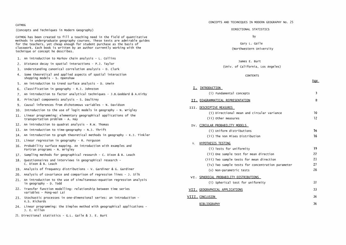
CONCEPTS AND TECHNIQUES IN MODERN GEOGRAPHY No. 25

DIRECTIONAL STATISTICS

by

Gary L. Gaile

(Northwestern University

James E. Burt

(Univ. of California, Los Angeles)

CONTENTS

I. INTRODUCTION

(i) Fundamental concepts

II. DIAGRAMMATICAL REPRESENTATION

III. DESCRIPTIVE MEASURES

(i) Directional mean and circular variance

(ii) Other measures

IV. CIRCULAR PROBABILITY MODELS

(i) Uniform distributions

(ii) The Von Mises Distribution

V. HYPOTHESIS TESTING

(i) Tests for uniformity

(ii) One sample test for mean direction

(iii) Two sample tests for mean direction

(iv) Two sample tests for concentration parameter

(v) Non-parametric tests

VI. SPHERICAL PROBABILITY DISTRIBUTIONS

(i) Spherical test for uniformity

VII. GEOGRAPHICAL APPLICATIONS

VIII. CONCLUSION

BIBLIOGRAPHY

Page

CATMOG

(Concepts and Techniques in Modern Geography)

CATMOG has been created to fill a teaching need in the field of quantitativemethods in undergraduate geography courses. These texts are admirable guidesfor the teachers, yet cheap enough for student purchase as the basis ofclasswork. Each book is written by an author currently working with thetechnique or concept he describes.

1. An introduction to Markov chain analysis - L. Collins

2. Distance decay in spatial interactions - P.J. Taylor

3. Understanding canonical correlation analysis - D. Clark

4. Some theoretical and applied aspects of spatial interactionshopping models - S. Openshaw

5. An introduction to trend surface analysis - D. Unwin

6. Classification in geography - R.J. Johnston

7. An introduction to factor analytical techniques - J.B.Goddard & A.Kirby

8. Principal components analysis - S. Daultrey

9. Causal inferences from dichotomous variables - N. Davidson

10. Introduction to the use of logit models in geography - N. Wrigley

11. Linear programming: elementary geographical applications of thetransportation problem - A. Hay

12. An introduction to quadrat analysis - R.W. Thomas

13. An introduction to time-geography - N.J. Thrift

14. An introduction to graph theoretical methods in geography - K.J. Tinkler

15. Linear regression in geography - R. Ferguson

16. Probability surface mapping. An introduction with examples andFortran programs - N. Wrigley

17. Sampling methods for geographical research - C. Dixon & B. Leach

18. Questionnaires and interviews in geographical research -C. Dixon & B. Leach

19. Analysis of frequency distributions - V. Gardiner & G. Gardiner

20. Analysis of covariance and comparison of regression lines - J. Silk

21. An introduction to the use of simultaneous-equation regression analysisin geography - D. Todd

22. Transfer function modelling: relationship between time seriesvariables - Pong-wai Lai

23. Stochastic processes in one-dimensional series: an introduction -K.S. Richards

24. Linear programming: the Simplex method with geographical applications -J. E. Killen

25. Directional statistics - G.L. Gaile & J. E. Burt

I INTRODUCTION

Direction is a geographical primitive. Together with distance it isimplicit in all spatial relationships. There are also many instances ingeography where explicit observations of direction are of interest. Recentadvances in mathematical statistics have provided rigorous techniques whichwill allow geographers explicitly to incorporate direction in their analyses.

Though arising quite naturally in geographical studies, directional dataoften behave strangely when subjected to the techniques commonly presentedin texts on quantitative geography. Even a technique as basic as computinga mean may lead to disturbing results. Suppose for example two observationsof wind direction are taken giving values of 45° and 315° with 0

0 as east.

The arithmetic mean of these two observations suggests that the averagewind direction is 180° (due west), a result which contradicts the intuitiveanswer of 0°. At first sight it might seem that the problem lies in the waydirection has been measured and that the solution is to transform thenumerical system of degrees into one which is suitable for traditional statis-tical analysis, but in actual fact it is the statistical techniques them-selves which require transformation to account for the special properties ofangular data. In the example above involving the mean of two angles theresults were dependent upon the choice of zero direction. Generally linearstatistics can be used with directional data only if the range of observationsis small (standard deviation less than 30

°) and the zero direction problem

obviated (Agterberg & Briggs, 1963).

The purpose of this monograph is to present a set of alternativetechniques which may be used when traditional analysis is not appropriate.Many of the concepts presented are analogous to those discussed in introduc-tory statistics texts and it is assumed the reader is familiar with thosetopics usually presented in first-year statistics, together with elementarytrigonometry. An excellent sourcebook and the stimulus for what follows isK.V. Mardia (1972).

(i) Fundamental Concepts

Traditional statistics are linear in the sense that variables areconsidered to be distributed on the number line. Movement from one end ofthe number line is movement towards the other end. In constructing ahistogram, for example, observations are measured with respect to a common(often arbitrary) origin and positions on the line are assigned to each.In directional statistics the observations are angles measured with respectto a reference direction or axis and the unit circle replaces the numberline. Each observation is positioned on the circumference of the circle sothat a vector joining the center of the circle and the observation formsan angle with reference axis equal to the observed angle (Figure 1).

In collecting observations on angular variables the reference (or zero)direction may be chosen purely for convenience; the only requirement isthat all observations be made using the same direction as zero. In thismonograph, as in most work in directional statistics, we will take the posi-tive x-axis as zero and measure all angles in a counterclockwise direction

Acknowledgements

The authors gratefully acknowledge the help of Kanti Mardia, William A.V.Clark, William Krumbein, and Susan Yardley. E. Batschelet and M.A.Stephens granted permission to use certain tables and figures.

3

Figure 2. Comparing polar coordinates and Cartesian coordinates.

5

Figure 1. The unit circle and the measurement of an angle.

The unit of measure of angles is also arbitrary so long as it isconsistent from observation to observation. In addition to the familiarsystem of degrees we will express angles in radians. The radian measure ofan angle is simply a dimensionless way of expressing its size. If a linesegment of length r is rotated about one of its end points through an angle

the ratio S divided by r. If the segment sweeps out an entire circle the

radian is approximately 57.3° (360°/2R).

Consider now an observation P on the circumference of a unit circle -a circle of radius one unit. Its position may be specified by its distancefrom the centre of the circle (one unit) together with its angular distance

to the positive x-axis allows one to convert from polar coordinates to the

4

its direction, in this case from 0 to P. This notation distinguishes avector from its length, in this case specified as simply OP. The vector is

vectors of unit length and operations are performed on the components of

an angle between 0 and 90 degrees. A constant is then added to the angle

Table 1. Constants to be used in determining the arctangent of an angle.

Sign of Numerator

The mechanics of the situation may be made clearer by considering thevectors to be successive movements of a particle. Vector A corresponds to

To find the direction of the resultant, therefore, one need only find

vector R has components:

by the Pythagorean Theorem:

In determining an arctangent care must be taken to observe the signs of the

Figure 3. A circular histogram of the Nairobi data.

7

II DIAGRAMMATICAL REPRESENTATION

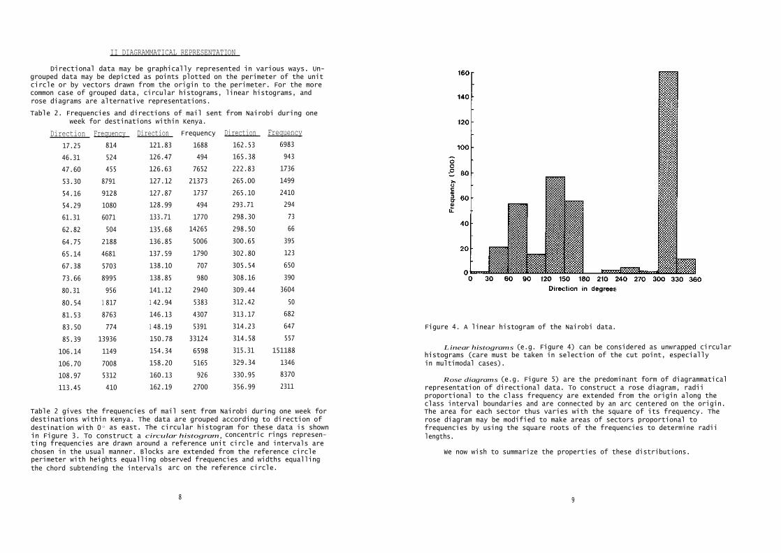
Directional data may be graphically represented in various ways. Un-grouped data may be depicted as points plotted on the perimeter of the unitcircle or by vectors drawn from the origin to the perimeter. For the morecommon case of grouped data, circular histograms, linear histograms, androse diagrams are alternative representations.

Table 2. Frequencies and directions of mail sent from Nairobi during oneweek for destinations within Kenya.

Table 2 gives the frequencies of mail sent from Nairobi during one week fordestinations within Kenya. The data are grouped according to direction ofdestination with 00 as east. The circular histogram for these data is shownin Figure 3. To construct a circular histogram, concentric rings represen-ting frequencies are drawn around a reference unit circle and intervals arechosen in the usual manner. Blocks are extended from the reference circleperimeter with heights equalling observed frequencies and widths equallingthe chord subtending the intervals arc on the reference circle.

8

Direction

17.25

Frequency

814

Direction

121.83

Frequency

1688

Direction

162.53

Frequency

6983

46.31 524 126.47 494 165.38 943

47.60 455 126.63 7652 222.83 1736

53.30 8791 127.12 21373 265.00 1499

54.16 9128 127.87 1737 265.10 2410

54.29 1080 128.99 494 293.71 294

61.31 6071 133.71 1770 298.30 73

62.82 504 135.68 14265 298.50 66

64.75 2188 136.85 5006 300.65 395

65.14 4681 137.59 1790 302.80 123

67.38 5703 138.10 707 305.54 650

73.66 8995 138.85 980 308.16 390

80.31 956 141.12 2940 309.44 3604

80.54 1 817 1 42.94 5383 312.42 50

81.53 8763 146.13 4307 313.17 682

83.50 774 1 48.19 5391 314.23 647

85.39 13936 150.78 33124 314.58 557

106.14 1149 154.34 6598 315.31 151188

106.70 7008 158.20 5165 329.34 1346

108.97 5312 160.13 926 330.95 8370

113.45 410 162.19 2700 356.99 2311

Figure 4. A linear histogram of the Nairobi data.

Linear histograms (e.g. Figure 4) can be considered as unwrapped circularhistograms (care must be taken in selection of the cut point, especiallyin multimodal cases).

Rose diagrams (e.g. Figure 5) are the predominant form of diagrammaticalrepresentation of directional data. To construct a rose diagram, radiiproportional to the class frequency are extended from the origin along theclass interval boundaries and are connected by an arc centered on the origin.The area for each sector thus varies with the square of its frequency. Therose diagram may be modified to make areas of sectors proportional tofrequencies by using the square roots of the frequencies to determine radiilengths.

We now wish to summarize the properties of these distributions.

9

( 3 )

and

Figure 5. A rose diagram of the Nairobi data.

III DESCRIPTIVE MEASURES

The example involving the mean of two angles showed that statisticscalculated using linear techniques are not appropriate in characterizing asample of angular observations. In this section several measures arepresented which can be used as directly analogous to measures which shouldbe familiar from linear statistics.

(i) Directional Mean and Circular Variance

It is ironic that the first arithmetic mean on record was calculated

10

that the centre of gravity of a set of points has coordinates equal to themean of the X coordinates and the mean of the Y coordinates; that is

(4)

( 5 )

Because

The mean direction possesses other interesting properties. For example,using the identities

(6)

(7)

it is not difficult to show that

(8)

( 9 )

The first property (equation 8), that deviates from the mean sum to

the sums of cosines of deviations to be maximized. For this very reason(9) is useful in characterizing the dispersion or spread of a sample. Infact the maximum given by (9) is actually the sample resultant length R..To see this use (7) to write

11

Circular variance is defined as

(10)

12 13

From Figure 2 it is seen that

thus

The resultant length R thus indicates the dispersion of a sample. For agroup of n vectors with identical directions,R will equal n and a sample ofperfectly opposing vectors would sum to zero. A large value of R therefore

indicates a dense bundle of vectors with small spread, and conversely forsmall R. In practice R is divided by n to facilitate comparison between

It sometimes happens that observations have 'sense' or orientation butnot direction. For example, one speaks of a road having a north-southorientation but a direction is not usually ascribed to the road in the way anautomobile travelling north on the road is said to have direction. Datapossessing orientation but not direction are called axial data or simply

orientation data. In a study of pebble orientation in sedimentary deposits,Krumbein (1939) showed that orientations may be converted to directionssimply by doubling the angles. This procedure yields the same angularmeasure for both components of the orientation.

(ii) Other Measures

Angular observations are often grouped into classes or segments of theunit circle. The U.S. Weather Service, for example, divides the circle intoeight classes of width 45° . A wind direction is reported according to theinterval within which it lies. The calculation of statistics for groupeddata is accomoplished by treating the observations of each class as if theyall fell at the class midpoint. Equations (4) and (5) may be used to find

Grouping a set of observations may bias an estimate slightly andto correct it perfectly it is necessary to apply a correction factor tostatistics other than the mean which have been calculated from grouped data.The correction is small, however, if the class interval is not large and mayusually be ignored as a matter of practice. For example, the correction toR is less than 3% for a class interval of 45

° (Mardia, 1972: 39).

Other descriptive measures such as median direction and circularmean deviation for directional data are shown in Table 4. In most casestheir calculation is straightforward and the meaning of each is comparableto that of its linear analog.

In closing this section we draw attention to the fact that thediscussion thus far has been confined to unit vectors. That is, only thedirection of the observations has been considered. All information concern-ing vector magnitudes is discarded when they are assigned unit length. Forexample, if wind speed and direction were measured only the direction 0would appear in the formulae given above.

magnitude by weighting each term in the summations according to an observat-ion's length. The resulting values would have clear physical interpretationbut statistical analysis as presented in the following sections would notbe possible. It is not difficult to see why this is so. Just as is thecase for linear statistics, directional statistical analysis is based onprobability density functions (p.d.f. ․ ). A p.d.f. is a non-negative functionwhose integral, extended over the entire x-axis in linear statistics and from0° to 360

° in directional statistics, is unity. The random variable

associated with a circular p.d.f. is an angle, and the function enables oneto make statements about the probability of observing particular angles. AsSteinmetz(1962) suggests, the use of vector lengths as weights involvespostulating that the longer a vector is, the more indicative of directionit is. It is more likely that vector length will appear in a geographicstudy as a random variable in its own right. To consider direction andmagnitude simultaneously would require a joint p.d.f.

We shall present only univariate distributions (indeed we know of nostudies using linear-directional bivariate p.d.f. ․ ). Returning to the ex-ample of wind speed and direction, it could be said that linear statisticswould enable one to investigate the marginal distribution of wind speed where-as the directional techniques presented here allow one to analyze the othermarginal.

IV CIRCULAR PROBABILITY MODELS

A large number of circular probability models exists; like linearprobability models, they may be either discrete or continuous. Several ofthe more important are discussed here.

Circular distribution functions and circular probability densityfunctions are defined in a manner similar to their linear counterparts. Con-sider a random variable X which is valued only on the circumference of a

Because

we may write

1514

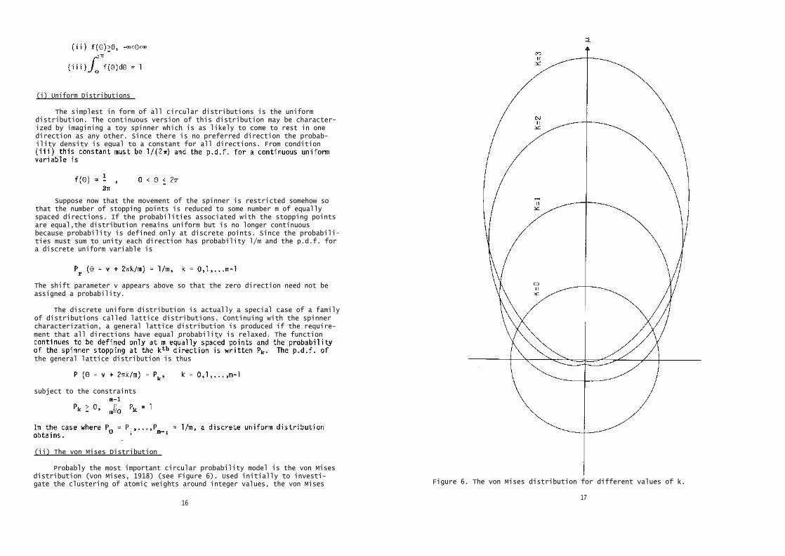
Figure 6. The von Mises distribution for different values of k.

17

(i) Uniform Distributions

The simplest in form of all circular distributions is the uniformdistribution. The continuous version of this distribution may be character-ized by imagining a toy spinner which is as likely to come to rest in onedirection as any other. Since there is no preferred direction the probab-ility density is equal to a constant for all directions. From condition

Suppose now that the movement of the spinner is restricted somehow sothat the number of stopping points is reduced to some number m of equallyspaced directions. If the probabilities associated with the stopping pointsare equal,the distribution remains uniform but is no longer continuousbecause probability is defined only at discrete points. Since the probabili-ties must sum to unity each direction has probability l/m and the p.d.f. fora discrete uniform variable is

The shift parameter v appears above so that the zero direction need not beassigned a probability.

The discrete uniform distribution is actually a special case of a familyof distributions called lattice distributions. Continuing with the spinnercharacterization, a general lattice distribution is produced if the require-ment that all directions have equal probability is relaxed. The function

the general lattice distribution is thus

subject to the constraints

(ii) The von Mises Distribution

Probably the most important circular probability model is the von Misesdistribution (von Mises, 1918) (see Figure 6). Used initially to investi-gate the clustering of atomic weights around integer values, the von Mises

16

distribution plays much the same role in circular statistical inference asthe Gaussian distribution does in linear statistics. It has two parameters -

(11)

where

ion so that (iii) is satisfied.

From (11) several important properties of the von Mises distributioncan be deduced which are analogous to those of the Gaussian. Like the linearnormal distribution it is completely determined by two parameters. The

symmetric about its mean.

The behaviour of (ii) under variation in k is also easy to see. As k

small values of k. Alternatively, as k grows large the distribution becomes

concentration parameter and it is somewhat analogous to the reciprocal ofthe normal distribution's variance.

Because of its pre-eminence in hypothesis testing, its characteristicscommon to the linear normal, and because it can be constructed as a condition-al distribution of the bivariate normal distribution, the von Mises is some-times called the 'circular normal distribution'. This name is somewhatimprecise for when a true linear normal distribution is extended directlyto the circle one obtains not a von Mises distribution but yet anothercircular distribution, the wrapped normal, which is important in the centrallimit theorem on the circle. In fact, the list of circular distributions islengthened considerably when it is realized that any linear distributionwith p.d.f. f(x) (continuous) or probability function p(x) (discrete) maybe wrapped around the circle by

and

respectively. Mardia (1972) discusses several wrapped distributions and

18

other circular distributions not mentioned here.

V HYPOTHESIS TESTING

A large number of inferential tests are available for variables distri-buted directionally, many of which are completely analogous to familiarlinear tests. In most cases assumptions about the parent distribution mustbe made, but a number of non-parametric tests exist which may be used whenassumptions about the population cannot be upheld. In this section, severalgeographical problems are analyzed to illustrate the variety and versatilityof hypothesis-testing techniques available in directional statistics. Unlessotherwise stated, the underlying population is assumed to approximate a vonMises distribution.

The procedure used in performing a test involving directional data isidentical to that used in linear statistics. The researcher forms a nullhypothesis which is tested against a mutually exclusive alternative hypothesis.The statistical theory on which the test is based allows one to reject thenull hypothesis with a known probability of error. The probability of errorassociated with retaining an untrue null hypothesis depends upon thealternate hypothesis and is in general unknown. For this reason hypothesesare usually formed with the experimenter playing the role of a prosecutortrying to prove the null hypothesis untrue.

(i) Tests for Uniformity

The first hypothesis-testing technique demonstrated addresses thequestion of whether there is a directional bias to the data. Tests of this

and there is no concentration around any particular direction.The Problem: Is the pattern of interaction around Nairobi directionallybiased? This type of problem is very common in spatial analyses. Tests foruniformity could be applied to hypotheses concerning von Thunen rings,Weberian transport costs, Christaller-type settlement patterns, or anyhypothesis involving an isotropic plane.The Data: The destinations within Kenya of all mail leaving Nairobi during oneweek were plotted. The directions of these destinations are the data andthe sample size is 63. The directions were measured by overlaying a pieceof transparent polar coordinate paper focussed on Nairobi but a protractorcould also be used. If the data had not been mapped but had been availablein Cartesian coordinates, the directions could have been determined bytrigonometric calculations based on the definitions that the cosine of the

are shown in Table 2.The Hypothesis: Given a von Mises distribution the hypothesis of uniformityis

19

the hypothesis of uniformity is rejected. There is evidence of directionalbias in the interactance pattern around Nairobi. The test outlined above

where C is the sum of the cosines of the angles (see Descriptive Measures section) and n is the size of the sample. A more detailed description ofthis test can be found in Stephens (1960).

5 0.413 0.522 0.611 0.7096 .376 .476 .560 .6527 .347 .441 .519 .6078 .324 .412 .486 .5699 .305 .388 .459 .538

10 .289 .368 .436 .51211 .275• .351 .416 .48912 .264 .336 .398 .46813 .253 .323 .383 .45114 .244 .311 .369 .43515 .235 .301 .357 .420

16 .228 .291 .345 .40717 .221 .282 .335 .3951 8 .215 .274 .326 .38419 .209 .267 .317 .37420 .204 .260 .309 .365

21 .199 .254 .302 .35622 .194 .248 .295 .34823 .190 .243 .288 .34124 .186 .238 .282 .33425 .182 .233 .277 .327

30 .17 .21 .25 .3035 .15 .20 .23 .2840 .14 .18 .22 .2645 .14 .17 .21 .2550 .13 .16 .20 .23

*Based on a table by Stephens with the kind permission of the author.

21

As was shown in Section 3, k is the concentration parameter of the vonMises distribution which is related (in a complex way) to circular variance.

5 0.677 0.754 0.816 0.879 0.9916 .618 .690 .753 .825 .9407 .572 .642 .702 .771 .8918 .535 .602 .660 .725 .8479 .504 .569 .624 .687 .808

10 .478 .540 .594 .655 .77511 .456 .516 .567 .627 .74312 .437 .494 .544 .602 .71613 .420 .475 .524 .580 .69214 .405 .458 .505 .560 .669

15 .391 .443 .489 .542 .64916 .379 .429 .474 .525 .63017 .367 .417 .460 .510 .61318 .357 .405 .447 .496 .59719 .348 .394 .436 .484 .583

20 .339 .385 .425 .472 .56921 .331 .375 .415 .461 .55622 .323 .367 .405 .451 .54423 .316 .359 .397 .441 .53324 .309 .351 .389 .432 .522

25 .303 .344 .381 .423 .51230 .277 .315 .348 .387 .47035 .256 .292 .323 .359 .43640 .240 .273 .302 .336 .40945 .226 .257 .285 .318 .386

50 .214 .244 .270 .301 .367100 .15 .17 .19 .21 .26

*Based on tables by Stephens and Batschelet with the kind permission ofthe authors.

Knowing (or assuming) the population to be von Mises allows the hypothesis of

20

(ii) One Sample Test for Mean Direction

This test asks whether the directional bias of the data clusters arounda specified direction. It is assumed that randomly sampled directions,

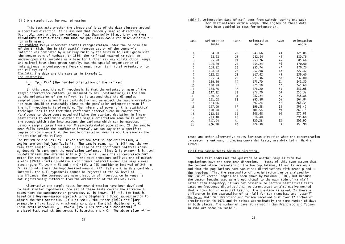
The Problem: Kenya underwent spatial reorganization under the colonialismof the British. The initial spatial reorganization of the country'sinterior was dominated by a railway built by the British to link Uganda withthe Kenyan port of Mombasa. In 1889, the railhead reached Nairobi, anundeveloped site suitable as a base for further railway construction. Kenyaand Nairobi have since grown rapidly. Has the spatial organization ofinteractance in contemporary Kenya changed from its initial orientation tothe railway axis?The Data: The data are the same as in Example 1.The Hypothesis:

In this case, the null hypothesis is that the orientation mean of theKenyan interactance pattern (as measured by mail destinations) is the sameas the orientation of the railway. It is assumed that the 63 anglessampled come from a von Mises distribution and we expect the sample orientat-ion mean should be reasonably close to the population orientation mean ifthe null hypothesis is plausible. The inferential power of this statisticaltechnique lies in the fact that confidence intervals can be constructed(analogous to those constructed utilizing the standard deviation in linearstatistics) to determine whether the sample orientation mean falls withinthe bounds which take into account the variance which can be expectedusing a sample taken from a von Mises-distributed population. If the samplemean falls outside the confidence interval, we can say with a specifieddegree of confidence that the sample orientation mean is not the same as theorientation of the railway.

meter for the population is unknown the test procedure utilizes one of Batsch-elet's (1971) charts to obtain a confidence interval around the sample mean(see Figure 7). As n = 63 and R = 0.4145, a 95% confidence interval of 246

° ±

27° is found. Since the hypothesized mean of 272

° falls within this confident

interval, the null hypothesis cannot be rejected at the 5% level ofsignificance. The contemporary mean direction of interactance in Kenya isnot significantly different from the orientation of the railway axis.

Alternative one sample tests for mean direction have been developedto test similar hypotheses. One set of these tests covers the infrequent

22

Table 7. Orientation data of mail sent from Nairobi during one weekfor destinations within Kenya. The angles of these datahave been doubled to test for orientation.

Case OrientationAngle

Case OrientationAngle

Case OrientationAngle

1 34.50 22 243.66 43 325.062 92.62 23 252.94 44 330.763 95.20 24 253.26 45 85.664 106.60 25 254.24 46 170.005 108.32 26 255.74 47 170.206 108.58 27 257.98 48 227.427 122.62 28 267.42 49 236.608 125.64 29 271.36 50 237.009 129.50 30 273.70 51 241.30

10 130.28 31 275.18 52 245.6011 134.76 32 276.20 53 251.0812 147.32 33 277.70 54 256.3213 160.62 34 282.24 55 258.8814 161.08 35 285.88 56 264.8415 163.06 36 292.26 57 266.3416 167.00 37 296.38 58 268.4617 170.78 38 301.56 59 269.16

1 8 212.28 39 308.68 60 270.6219 213.40 40 316.40 61 298.6820 217.94 41 320.26 62 301.9021 226.90 42 324.38 63 353.98

tests and other alternative tests for mean direction when the concentrationparameter is unknown, including one-sided tests, are detailed in Mardia(1972).

(iii) Two Sample Tests for Mean Direction

This test addresses the question of whether samples from twopopulations have the same mean direction. Tests of this type assume thatthe concentration parameters of the two populations, k1 and k2 are equaland that the populations have von Mises distributions with means p and 1-1 2

The Problem: That the seasonality of precipitation can be analyzed bythe use of vector lengths has been shown by Markham (1970), but becausethe vector lengths used were proportional to the magnitude of rainfallrather then frequency, it was not possible to perform statistical testsbased on frequency distributions. To demonstrate an alternative methodthat allows for inferential testing, the question is asked, Is there adifference in the seasonality of rainfall for San Francisco and Tucson?"The Data: Both San Francisco and Tucson received just over 12 inches ofprecipitation in 1971 and it rained approximately the same number of daysin both places. The number of days it rained in San Francisco and Tucsonin 1961 are shown in Table 8.

23

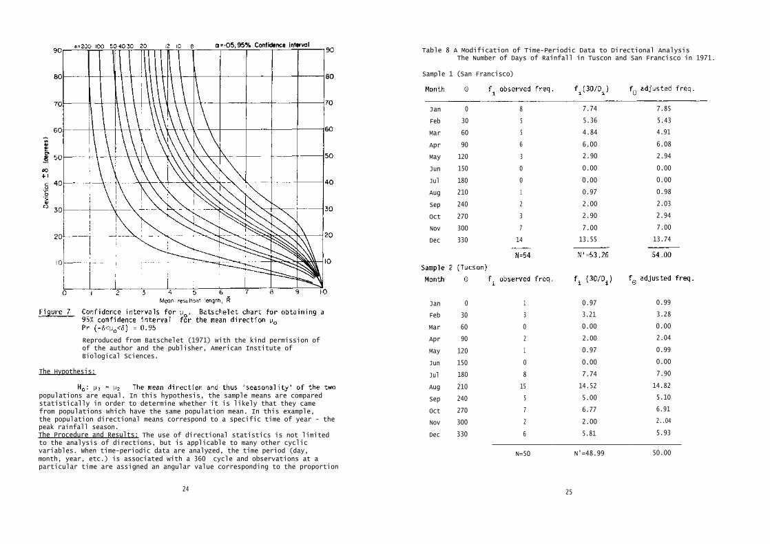
Jan 0 8 7.74 7.85

Feb 30 5 5.36 5.43

Mar 60 5 4.84 4.91

Apr 90 6 6.00 6.08

May 120 3 2.90 2.94

Jun 150 0 0.00 0.00

Jul 180 0 0.00 0.00

Aug 210 1 0.97 0.98

Sep 240 2 2.00 2.03

Oct 270 3 2.90 2.94

Nov 300 7 7.00 7.00

Dec 330 14 13.55 13.74

Reproduced from Batschelet (1971) with the kind permission ofof the author and the publisher, American Institute ofBiological Sciences.

The Hypothesis:

populations are equal. In this hypothesis, the sample means are comparedstatistically in order to determine whether it is likely that they camefrom populations which have the same population mean. In this example,the population directional means correspond to a specific time of year - thepeak rainfall season.The Procedure and Results: The use of directional statistics is not limitedto the analysis of directions, but is applicable to many other cyclicvariables. When time-periodic data are analyzed, the time period (day,month, year, etc.) is associated with a 360

° cycle and observations at a

particular time are assigned an angular value corresponding to the proportion

24

Table 8 A Modification of Time-Periodic Data to Directional AnalysisThe Number of Days of Rainfall in Tuscon and San Francisco in 1971.

Sample 1 (San Francisco)

Jan 0 1 0.97 0.99

Feb 30 3 3.21 3.28

Mar 60 0 0.00 0.00

Apr 90 2 2.00 2.04

May 120 1 0.97 0.99

Jun 150 0 0.00 0.00

Jul 180 8 7.74 7.90

Aug 210 15 14.52 14.82

Sep 240 5 5.00 5.10

Oct 270 7 6.77 6.91

Nov 300 2 2.00 2..04

Dec 330 6 5.81 5.93

N=50 N'=48.99 50.00

25

Since for a fixed resultant of the combined sample (R), the sum of the

26

The statistic G is approximately normally distributed with mean zeroand variance unity:

27

Table 8 (continued)

Combined Sample

Jan 0 9 8.71 8.86

Feb 30 8 8.57 8.72

Mar 60 5 4.84 4.92

Apr 90 8 8.00 8.14

May 120 4 3.87 3.94

Jun 150 0 0.00 0.00

Jul 180 8 7.74 7.87

Aug 210 16 15.48 15.75

Sep 240 7 7.00 7.12

Oct 270 10 9.68 9.84

Nov 300 9 9.00 9.15

Dec 330 20

N=104

10.35

N'.102.25

19.68

104.00

(12)

When the data are grouped by month, the frequencies must be adjusted toaccount for the inequality of class intervals. This can be accomplishedby creating a new year of 360 days having twelve months of thirty dayseach. The adjusted frequencies are found by:

where k is estimated by the use of Gumbel's (1954) Table 2 or Batschelet's(1971) Table B.

thus the hypothesis of equal mean directions is strongly rejected; it isconcluded that a seasonal difference exists in the precipitation patternsof the two locations.

(iv) Two Sample Tests for Concentration Parameter

This test addresses the question of whether the circular variances of

a von Mises distribution.The Problem: The analysis of river meanders is an important aspect offluvial geomorphology which has not been wholly integrated into the theoryof river systems. Most sinuosity indices (Mueller, 1968) of river meandersdo not measure the fundamental aspect of meander-changes in direction. Itis proposed here that the circular variance be used as a testable index ofstream meanders. For example, is the meander pattern of a plains river(the Little Missouri) different from the meander pattern of a mountainriver (the Klamath)?The Data: From the U.S.G.S. 1:24000 maps of the Klamath and Little Missouririvers, a starting point and fifty sample points at 1000 feet intervalsupstream were chosen for each river. Using a method similar to that ofThakur and Scheidegger (1968), each midstream point was linked to itsneighbour by astraight line whose direction was found relative to the directionof the main valley axis.The Hypothesis:

Table 9 Hypothetical Preferred Directions of Prospective Brides by17 Mysoreian Villagers

28 29

thus G = 3.853 which is greater than a critical value at the 95% levelof 1.96 and the null hypothesis is rejected. The two rivers have differentmeander patterns.

(v) Non-Parametric Tests

Except for the test for uniformity, the tests presented thus farrequire the assumption that the underlying population can be representedby a von Mises distribution. In directional statistics, as in linearstatistics, situations arise in which such assumptions about the form ofthe parent population are untenable. Fortunately, a variety of non-parametricdirectional tests exists which affords a fair amount of flexibility to theresearcher.The Problem: It has been suggested that the 'ritual custom of agni mullwhich prohibits the taking of a wife from the southeast or northwest of one'sown village' has affected mate selection in Mysoreian villages (McCormack,1958). Could directional statistics be used to test the adherence to thiscultural taboo?The Data: Table 9 presents hypothetical responses from 17 villagers to thequestion: 'Which direction would you prefer your wife to come from?'The Hypothesis:

The Procedure and Results: Single sample tests usually fall into one oftwo categories tests for uniformity and tests for symmetry. In testing thehypothesis that a distribution is symmetric about a given direction, it ispossible to use symmetry tests adapted from linear statistics. Schach (1969)has outlined the use of the Wilcoxon test for circular data and discussedits efficiency relative to tests for von Mises populations. The sign testwas evaluated in a similar manner and found to be more powerful than theWilcoxon test for small k and large n.

1 40 .111 .059 .052

2 54 .150 .118 .032

3 73 .203 .176 .027

4 85 .236 .235 .001

5 92 .256 .294 -.038

6 114 .317 .353 -.036

7 154 .428 .412 .016

8 170 .472 .471 .001

9 178 .494 .529 -.035

10 191 .531 .588 -.057

11 220 .611 .647 -.036

12 248 .689 .706 -.017

13 280 .778 .765 .013

14 293 .814 .824 -.010

15 307 .853 .882 -.029

16 321 .892 .941 -.049

17 346 .961 1.000 -.039

Stephens (1969b) has compared the relative power of the three tests using

Monte Carlo trials. Although the power of a test varies with the alternativeconsidered, in general it can be said that Kuiper's V-test is preferred,particularly for small samples.

Kuiper's test is similar to the Kolmogorov-Smirnov test in that it isbased on the maximum deviations of the observed distribution from theexpected. Following Mardia (1972, ch.7), a distribution function of fixedzero direction is defined by:

and

Testing at the 5% level, the critical value is 1.66 for n=17 and thus thenull hypothesis is not rejected. The cultural taboo is not validated bythe data.

VI SPHERICAL PROBABILITY DISTRIBUTIONS

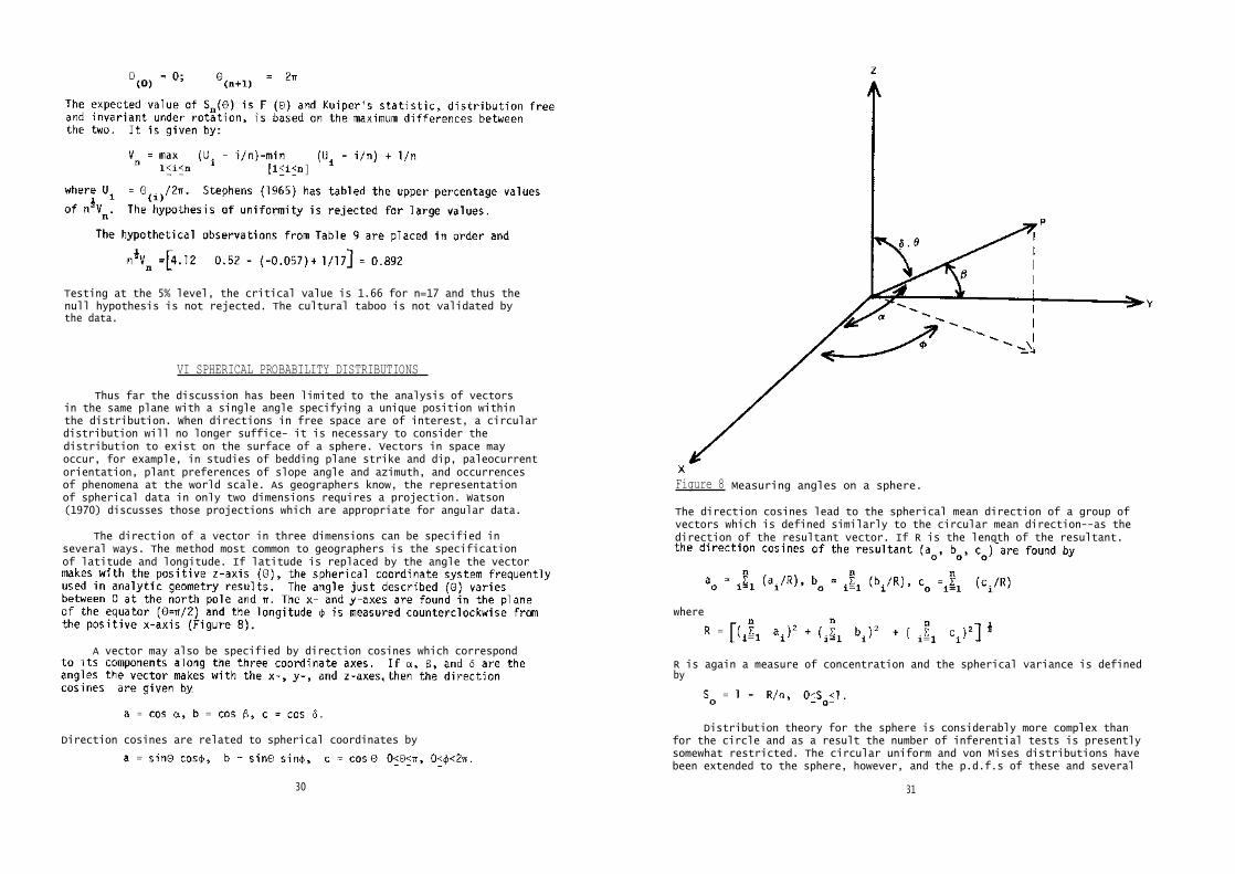
Thus far the discussion has been limited to the analysis of vectorsin the same plane with a single angle specifying a unique position withinthe distribution. When directions in free space are of interest, a circulardistribution will no longer suffice- it is necessary to consider thedistribution to exist on the surface of a sphere. Vectors in space mayoccur, for example, in studies of bedding plane strike and dip, paleocurrentorientation, plant preferences of slope angle and azimuth, and occurrencesof phenomena at the world scale. As geographers know, the representationof spherical data in only two dimensions requires a projection. Watson(1970) discusses those projections which are appropriate for angular data.

The direction of a vector in three dimensions can be specified inseveral ways. The method most common to geographers is the specificationof latitude and longitude. If latitude is replaced by the angle the vector

Figure 8 Measuring angles on a sphere.

The direction cosines lead to the spherical mean direction of a group ofvectors which is defined similarly to the circular mean direction--as thedirection of the resultant vector. If R is the length of the resultant.

where

A vector may also be specified by direction cosines which correspondR is again a measure of concentration and the spherical variance is definedby

Direction cosines are related to spherical coordinates by

30

Distribution theory for the sphere is considerably more complex thanfor the circle and as a result the number of inferential tests is presentlysomewhat restricted. The circular uniform and von Mises distributions havebeen extended to the sphere, however, and the p.d.f.s of these and several

31

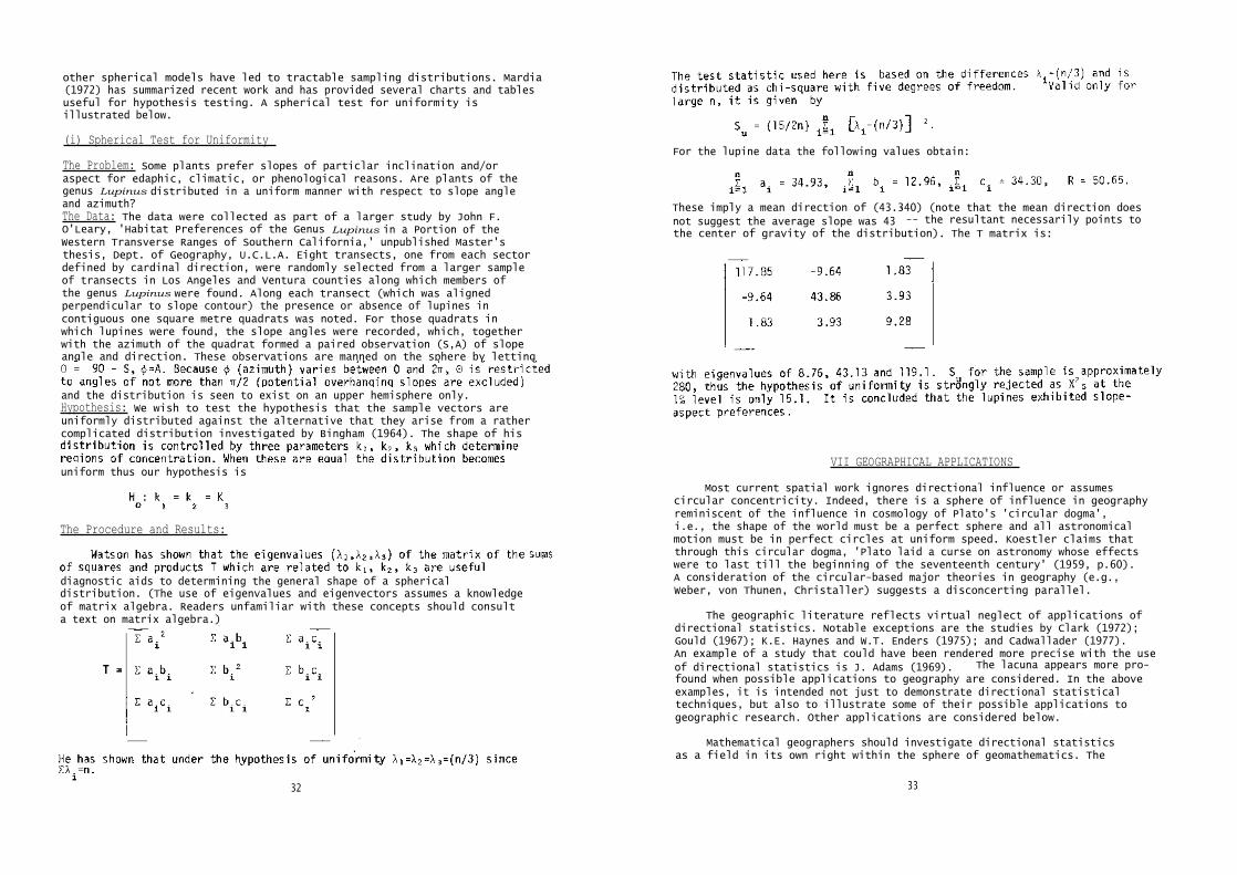
other spherical models have led to tractable sampling distributions. Mardia(1972) has summarized recent work and has provided several charts and tablesuseful for hypothesis testing. A spherical test for uniformity isillustrated below.

(i) Spherical Test for Uniformity

The Problem: Some plants prefer slopes of particlar inclination and/oraspect for edaphic, climatic, or phenological reasons. Are plants of thegenus Lupinus distributed in a uniform manner with respect to slope angleand azimuth?The Data: The data were collected as part of a larger study by John F.O'Leary, 'Habitat Preferences of the Genus Lupinus in a Portion of theWestern Transverse Ranges of Southern California,' unpublished Master'sthesis, Dept. of Geography, U.C.L.A. Eight transects, one from each sectordefined by cardinal direction, were randomly selected from a larger sampleof transects in Los Angeles and Ventura counties along which members ofthe genus Lupinus were found. Along each transect (which was alignedperpendicular to slope contour) the presence or absence of lupines incontiguous one square metre quadrats was noted. For those quadrats inwhich lupines were found, the slope angles were recorded, which, togetherwith the azimuth of the quadrat formed a paired observation (S,A) of slopeangle and direction. These observations are manned on the sphere by letting

and the distribution is seen to exist on an upper hemisphere only.Hypothesis: We wish to test the hypothesis that the sample vectors areuniformly distributed against the alternative that they arise from a rathercomplicated distribution investigated by Bingham (1964). The shape of his

uniform thus our hypothesis is

The Procedure and Results:

diagnostic aids to determining the general shape of a sphericaldistribution. (The use of eigenvalues and eigenvectors assumes a knowledgeof matrix algebra. Readers unfamiliar with these concepts should consulta text on matrix algebra.)

32

For the lupine data the following values obtain:

These imply a mean direction of (43.340) (note that the mean direction doesnot suggest the average slope was 43

°-- the resultant necessarily points to

the center of gravity of the distribution). The T matrix is:

VII GEOGRAPHICAL APPLICATIONS

Most current spatial work ignores directional influence or assumescircular concentricity. Indeed, there is a sphere of influence in geographyreminiscent of the influence in cosmology of Plato's 'circular dogma',i.e., the shape of the world must be a perfect sphere and all astronomicalmotion must be in perfect circles at uniform speed. Koestler claims thatthrough this circular dogma, 'Plato laid a curse on astronomy whose effectswere to last till the beginning of the seventeenth century' (1959, p.60).A consideration of the circular-based major theories in geography (e.g.,Weber, von Thunen, Christaller) suggests a disconcerting parallel.

The geographic literature reflects virtual neglect of applications ofdirectional statistics. Notable exceptions are the studies by Clark (1972);Gould (1967); K.E. Haynes and W.T. Enders (1975); and Cadwallader (1977).An example of a study that could have been rendered more precise with the useof directional statistics is J. Adams (1969). The lacuna appears more pro-

found when possible applications to geography are considered. In the aboveexamples, it is intended not just to demonstrate directional statisticaltechniques, but also to illustrate some of their possible applications togeographic research. Other applications are considered below.

Mathematical geographers should investigate directional statisticsas a field in its own right within the sphere of geomathematics. The

33

techniques may have further applications to the study of shape, pattern,and orientation. The quantitative analysis of shape is dominated by indicescalculated from distances (measured along radials, axes, or perimeters) andoften requiring the index to be relative to geometric shapes or shape suchas a circle or polygon. It might be possible to use Taylor's (1971) methodof overlaying a rectangular grid of points on the shape, and, rather thanmeasuring the distance from each circumscribed point to all other circum-scribed points, measure the direction (irrespective of initial orientation).The circular variance of the measured directions may be a useful alternativemeasure of shape and has the additional asset of being easily testedinferentially. Pattern has been analyzed through quadrat analysis, Lexisnumbers, and near-neighbor analysis - all distance-based statistics (withquasi-directional variation by Dacey and Tung, 1962). Only recently havedirectional characteristics of point patterns been analyzed (Haynes andEnders, 1975; Boots, 1974). The quantitative assessment of orientation,often attempted obliquely (Blair and Bliss, 1967), is definitively resolvedwith the use of directional statistics. Should geomathematicians manage totransfer the techniques of circular regression and vector trend surfaceanalysis from exploratory to operational status, the range of possibleapplications throughout the spatial sciences would be considerably increased.

Urban-economic geographers will find directional statistics complementaryto their existing base of structural research as well as to more contemporarydynamic concerns. Transport networks have definite directional attributesthat have been woefully neglected in research predominantly utilizinggraph-theoretic methodology. Using frequencies to depict magnitudes andchanges of flows, directional statistics can accomodate dynamic analysesof transport.

The dynamic notions of changing urban forms have been voiced in avariety of speculations from the historical evolution of Gottmann's (1961)'Megalopolis' through Friedmann and Miller's (1965) more general 'urbanfields'. Are cities represented by their delineated forms growing towardseach other (is there evidence for urban 'gravity')? Directional statisticscould test whether the growth of urban form is directionally biased towardsother urban areas. (A pilot study by one of the authors did not supportthis hypothesis.) Directional statistics can be applied to central placestudies. Mardia (1972) discusses theoretical lattice distributions that maybe well-suited to central place analysis and particularly to the Losch (1954)variant.

The urban-structural debate of Hoyt's (1933) sectors versus Burgess's(1925) rings has continued for decades. Comparative analysis of the twomodels has often been inconclusive, although Yeates (1965) was able todemonstrate the importance of direction on land value prediction by analysisalong individual sectors. Directional statistics could assist in theclarification of this dilemma. The generalized land surface values withina city posited by Berry et al. (1963) can be seen to have definite directionalattributes. Studies of urban-hinterland development surfaces have alsoisolated strong directional components.

Both Weber's and von Thunen's models are based on transport costswhich vary radically with respect to distance, depending on the existenceof transport arteries (von Thunen explicitly recognized this), yet themodels are most usually employed incorporating an assumption of concentric

34

transport costs. Hamilton (1967), in his concentric model of theindustrial structure of a metropolis, notes 'the 'wedging' effect oftransport lines on the distribution pattern'. The explicit incorporationof direction into these and similar models may be detrimental to theirelegance, but not to their utility.

Human geographers will find directional statistics an aid to theiranalyses of diffusion. Agricultural dispersions usually display a preferreddirection relative to their origin. Diffusion models are often concentric('wave-like') or hierarchic (essentially aspatial), but seldom directional.The mean information fields of Monte Carlo simulation of diffusion may bemodified to employ a polar-coordinate field, with probability values varyingin relation to theoretically- or empirically-derived mean direction andcircular variance. An example of the directional bias of diffusion can beseen in the analysis of Kenya mail data in Example 1 and 2. Cadwallader(1977) has used directional statistics to determine directional biases (framedependency) in cognitive maps.

Biogeographers and mathematical ecologists will find a variety of usesfor the techniques. Organisms not only diffuse non-randomly, but alsowith preferred direction. Zoogeographers will find that zoologists andethologists have already applied directional statistics to the migrationand orientation behaviour of ducks, turtles, and homing pigeons- the latterstudy offering the less-then-startling conclusion that homing pigeons flyhome. Plant geographers should note the application of the spherical(three-dimensional) techniques to the relationship between plant distributionsand physical features shown in Example 6.

The use of directional statistics has been more widespread in studiesallied to physical geography. The most common application has been in thestudy of bedding plane and grain axis orientation with the majority ofreferences appearing in the geologic rather than geographic literature (e.g.,Scheidegger, 1965; Williams, 1972; Mark, 1973). Steinmetz(1962) has tabledsome of the uses to which directional statistics have been put; otherreviews may be found in Jones (1968) and Pincus (1956).

Since many climatological processes are time-periodic (e.g., Example3), they are amenable to analysis using directional techniques. Otherclimatological applications include the study of wind directions which hasbeen preliminarily explored by meteorologists. Their initial researchindicates that the distributions of wind directions can be closely approxi-mated by a particular bivariate circular probability density function, butmuch inferential work remains to be done using this model.

Extending his wind power studies, Hardy (1977) has developed a new way

ized as in ordinary principal components analysis. In the case of Hardy'swork this has resulted in the delineation of regional wind patterns. Thetechnique has obvious potential application to other vector fields and itsrelationship to the techniques 'presented here should be examined.

35

VIII CONCLUSION

Directional statistics have been introduced as a set of techniqueswith considerable potential application to geographical research. Giventhat direction is an explicitly spatial concept, the adoption of thesetechniques by geographers will facilitate the inclusion of this geographicalprimitive into their analyses. As with linear statistics, an understandingof theory and models underlying directional statistics requires considerablemastery of mathematics, yet the simple application of the variety ofmathematically acceptable tests demonstrated in the examples of this workis not predicated on such mastery.

The fact that geographers have not rigorously included direction intheir research is understandable given the dominant use of linear statisticsin science. That a linear rather than a directional theory of statisticsdeveloped is ironical given the genesis of the arithmetic mean and thetheory of errors:

Indeed the theory of errors was developed by Gaussprimarily to analyze certain directional measurementsin astronomy. It is a historical accident that theobservational errors were sufficiently small to allowGauss to make a linear approximation and, as a result,he developed a linear rather than a directional theoryof errors (Mardia, 1972, p.xvii).

It is recommended that geographers be among the first to redirect theirapproach to quantitative analyses from the straight and narrow path ofhistorical accident.

BIBLIOGRAPHY

GENERAL

Fisher, R.A., (1959), Statistical Methods and Scientific Inference.(Edinburgh: Oliver & Boyd).

Gottman, J., (1961), Megalopolis. (N.Y.: Twentieth Century Fund).

Hoyt, H., (1933), One Hundred Years of Land Values in Chicago.(Chicago: Univ. of Chicago Press).

Koestler, A., (1959), The Sleepwalkers (N.Y.: MacMillan)

Losch, A., (1954), The Economics of Location . (New Haven: YaleUniversity Press).

THEORY

Ajne, B., (1968), A Simple Test for Uniformity of a Circular Distribution.Biometrika, 55, 343-54.

Batschelet, E., (1971), Recent Statistical Methods for Orientation Data.Animal Orientation, Symposium 7970 on Wallops Island.American Institute Biological Sciences. Washington.

36

Beran, R.J., (1969), Asymptotic theory of a class of tests for uniformityof a circular distribution. Annals of mathematicalStatistics, 40, 1196-1206.

Bingham, C., (1964), Distributions on the sphere and on the projectiveplane. Ph. D. Thesis. Yale University.

Blais, D.J. & Biss, T.H., (1967), The Measurement of shape in geography:an appraisal of methods and techniques. Bulletin of Quantit-ative Data for Geographers, Dept. of Geography, 11,Nottingham University.

Boots, B.N., (1974), Delauney triangles: an alternative approach to pointpattern analysis. Proceedings of the Association ofAmerican Geographers, 6, 26-29.

Dacey, M.F. & Tung, T., (1962), The identification of randomness in pointpatterns. Journal of Regional Science, 4, 83-96.

Gould, P.R., (1967), On the Geographical interpretation of eigenvalues .Transactions of the Institute of British Geographers,42, 53-86.

Gumbel, E.J., (1954), Applications of the circular normal distribution.Journal of the American Statistical Association,49, 267-297.

Jones, J.A., (1968), Statistical analysis of orientation data. Journal ofSedimentary Petrology, 38, 61-67.

Kuiper, N.H., (1960), Tests concerning random points on a circle. Ned.Akad. Wet. Proc., A63, 38-47.

Mardia, K.V., (1972), Statistics of Directional Data (N.Y.:Academic Press).

Mark, D.M., (1973), Analysis of axial orientation data, including tillfabrics. Bulletin Geological Society of America,84, 1369-74.

Mueller, J.E., (1968), An introduction to the hydraulic and topographicsinuosity indexes, Annals of the Association of AmericanGeographers, 58, 371-385.

Pincus, H.J., (1956), Some vector and arithmetic operations on two-dimens-ional orientation variates, with applications to geologic data.Journal of Geology, 64, 533-57.

Rayleigh, L., (1919), On the problem of random vibrations, and of randomflights in one, two, or three dimensions. Philosophical

magazine,37, 321 -47.

Schach, S., (1969), On a class of non-parametric two-sample tests forcircular distributions. Annals of Mathematical Statistics,40, 1791-800.

Scheidegger, A.E., (1965), On the statistics of the orientation of beddingplanes grain axes, and similar sedimentological data.U.S. Geological Survey Professional Paper, 525-C, C-164-67.

Steimitz, R., (1962), Analysis of vectoral data. Journal of Sedimentary

Petrology, 32, 801-17.

37

Stephens, M.A., (1965), The goodness-of-fit statistic V n : distribution andsignificance points. Biometrika, 52, 309-21.

Stephens, M.A., (1969b), A goodness-of-fit statistic for the circle, withsome comparisons. Biometrika, 56, 161-68.

Von Mises, R., (1968), Uber die 'Ganzzahligkeit' der Atomogewicht andverwandte Fragen. Physika Zeitschrift, 19, 490-500.

Watson, G.S., (1970), Orientation statistics in the earth sciences.Bulletin of the Geological Institutions of Universityof Uppsala, 2, 73-89

Watson, G.S. & Williams, E.J., (1956), On the construction of significancetests on the circle and the sphere. Biometrika, 43.

APPLIED

Adams, J., (1969), Directional Bias in Intra-Urban Migration. EconomicGeography, 45, 302-323.

Agterberg, F.P. & Briggs, G., (1963), Statistical Analysis of Ripple Marksin Atokan and Desmoinesian Rocks in the Arkoma Basin ofEastcentral Oklahoma. Journal of Sedimentary Petrology,33, 343-410.

Berry, B.J.L.; Tennant, R.S.; Garner, B.J. & Simmons, J.W., (1963),Commercial Structure and Commercial blight. (Chicago: universityof Chicago, Dept. of Geography, Resource Paper, 85).

Burgess, E.W., (1925), The growth of the city: an introduction to a researchproject. In The City, eds. R.E. Park, E.W. Burgess and R.D.McKenzie, (Chicago: Univ. of Chicago Press).

Cadwallader, M., (1977), Frame dependency in cognitive maps: analysis usingdirectional statistics. Geographical Analysis, 9, 284-292.

Clark, W.A.V., (1972), Some vector representations of intra-urbanresidential mobility. International Geography, 2, 796-798.

Friedmann, J. & Miller, J., (1965), The urban field. Journal of theAmerican Institute of Planners, 31, 312-319.

Hamilton, F.E.I., (1967), Models of industrial location. In Models inGeography, eds. R.J. Chorley & P. Haggett, (London: Methuen).

Hardy, D.M., (1977), Empirical Eigenvector Analysis of Vector Observations,Geophysical Research Letters, 4, 319-320.

Haynes, K.E. & Enders, W.T., (1975), Distance, direction, and entropy in theevolution of a settlement pattern. Economic Geography,51, 357-65.

Krumbein, W.C., (1939), Preferred orientation of pebbles in sedimentarydeposits. Journal of Sedimentary Petrology, 47,673-706.

Markham, C.C., (1970); Seasonality of precipitation in the United StatesAnnals of the Association of American Geographers,60, 592-97.

McCormack, W., (1958), Sister's daughter marriage in a Mysore Village.Man in India, 38.

38

Taylor, P.J., (1971), Distances within shapes: an introduction to a familyof finite frequency distributions. Geografiska Annaler,

53B, 4-53.

Thakur, B. & Scheidegger, A.E., (1968), A test for the statistical theory ofmeander formation. Water Resources Research, 4, 317-29.

Williams, P.W., (1972), Morphometric Analysis of polygonal karst in NewGuinea, Geological Society of American Bulletin,83,761-796.

Yeates, M., (1965), Some factors affecting the spatial distribution ofChicago land values. Economic Geography, 41, 57-70.

39

This series, Concepts and Techniques in Modern Geographyis produced by the Study Group in Quantitative Methods, ofthe Institute of British Geographers.For details of membership of the Study Group, write tothe Institute of British Geographers, 1 Kensington Gore,London, S.W.7.The series is published by Geo Abstracts, University ofEast Anglia, Norwich, NR4 7TJ, to whom all other enquiriesshould he addressed.