Direction-of-change forecasts based on conditional ...fdiebold/papers/paper73/CDMTT.pdf · Roberto...

Direction-of-change forecasts based onconditional variance, skewness and kurtosisdynamics: international evidence

Peter F. ChristoffersenDesautels Faculty of Management, McGill University, 1001 Sherbrooke Street West,Montreal, Quebec H3A1G5, Canada; email: [email protected], School of Economics and Management, University of Aarhus, Building 1322, DK-8000 AarhusC, Denmark

Francis X. DieboldDepartment of Economics, University of Pennsylvania, 3718 Locust Walk, Philadelphia,PA1914-6297, USA; email: [email protected], 1050 Massachusetts Avenue, Cambridge, MA 02138-5398, USA

Roberto S. MarianoSchool of Economics and Social Sciences, Singapore Management University, 90 Stanford Road, Singapore, 178903; email: [email protected]

Anthony S. TaySchool of Economics and Social Sciences, Singapore Management University, 90 Stanford Road, Singapore, 178903; email: [email protected]

Yiu Kuen TseSchool of Economics and Social Sciences, Singapore Management University, 90 Stanford Road, Singapore, 178903; email: [email protected]

Recent theoretical work has revealed a direct connection between assetreturn volatility forecastability and asset return sign forecastability. Thissuggests that the pervasive volatility forecastability in equity returnscould, through induced sign forecastability, be used to produce direction-of-change forecasts useful for market timing. We attempt to do so in an

123456789

10111213141516171819202122232425262728293031323334353637383940414243

44N

Journal of Financial Forecasting (1–22) Volume 1/ Number 2, Fall 2007

1

This work was supported by FQRSC, IFM2, SSHRC (Canada), the National Science Founda-tion, the Guggenheim Foundation, the Wharton Financial Institutions Center (US) andWharton – Singapore Management University Research Centre. We thank participants of the9th World Congress of the Econometric Society and numerous seminars for comments, but weemphasize that any errors remain ours alone.

JFF 07 08 06 PC 10/26/07 1:21 PM

international sample of developed equity markets, with some success, asassessed by formal probability forecast scoring rules such as the Brierscore. An important ingredient is our conditioning not only on conditionalmean and variance information, but also on conditional skewness andkurtosis information, when forming direction-of-change forecasts.

1 INTRODUCTION

Recent work by Christoffersen and Diebold (2006) has revealed a direct connec-tion between asset return volatility dependence and asset return sign dependence(and hence sign forecastability). This suggests that the pervasive volatilitydependence in equity returns could, through induced sign dependence, be used toproduce direction-of-change forecasts useful for market timing.

To see this, let Rt be a series of returns and �t be the information set available attime t. Pr[Rt � 0] is the probability of a positive return at time t. The conditionalmean and variance are denoted, respectively, as �t�1|t � E[Rt�1��t] and �2

t�1�t �

Var[Rt�1��t]. The return series is said to display conditional mean predictabilityif �t�1�t varies with �t; conditional variance predictability is defined similarly.If Pr[Rt � 0] exhibits conditional dependence, ie, Pr[Rt�1 � 0��t] varies with �t,then we say the return series is sign predictable (or the price series is direction-of-change predictable).

For clearer exposition, and to emphasize the role of volatility in return sign pre-dictability, suppose that there is no conditional mean predictability in returns, so�t�1�t � � for all t. In contrast, suppose that �2

t�1�t varies with t in a predictablemanner, in keeping with the huge literature on volatility predictability reviewed inAndersen et al (2006). Denoting D(�,� 2) as a generic distribution dependent onlyon its mean � and variance �2, assume

Then the conditional probability of positive return is

(1)

where F is the distribution function of the “standardized” return (Rt�1�t �

�)/�t�1�t). If the conditional volatility is predictable, then the sign of the return is

� 1 � F � � �

�t�1�t�

� 1 � Pr�Rt�1 � �

�t�1� t

� �

�t�1� t�

Pr(Rt�1 � 0 � �t) � 1 � Pr(Rt�1 0 � �t)

Rt�1��t ~ D(�,�2t�1�t)

1234567891011121314151617181920212223242526272829303132333435363738394041424344N

Journal of Financial Forecasting Volume 1/ Number 2, Fall 2007

P. F. Christoffersen et al2

JFF 07 08 06 PC 10/26/07 1:21 PM

predictable even if the conditional mean is unpredictable, provided � 0. Notealso that if the distribution is asymmetric, then the sign can be predictable evenif the mean is zero: time-varying skewness can be driving sign prediction inthis case.

In practice, interaction between mean and volatility can weaken or strengthenthe link between conditional volatility predictability and return sign predictability.For instance, time variation in conditional means of the sort documented in recentwork by Brandt and Kang (2004) and Lettau and Ludvigson (2005) wouldstrengthen our results. Interaction between volatility and higher-ordered condi-tional moments can similarly affect the potency of conditional volatility as apredictor of return signs.

In this paper, we use

(2)

to explore the sign predictability of one-, two- and three-month returns in threestock markets,1 in which we examine out-of-sample predictive performance. Wealso use an extended version of Equation (2) that explicitly considers the interac-tion between volatility and higher-ordered conditional moments. We estimate theparameters of the models recursively and we evaluate the performance of signprobability forecasts. We proceed as follows: in Section 2, we discuss our data andits use for the construction of volatility forecasts; in Section 3, we discuss ourdirection-of-change forecasting models and evaluation methods; in Section 4, wepresent our empirical results; and in Section 5, we conclude.

2 DATA AND VOLATILITY FORECASTS

Estimates and forecasts of realized volatility are central to our analysis; for back-ground, see Andersen et al (2003, 2006). Daily values for the period 1980:01 to2004:06 of the MSCI index for Hong Kong, UK and US were collected fromDatastream. From these, we constructed one-, two- and three-month returns andrealized volatility. The latter is computed as the sum of squared daily returnswithin each one-, two- and three-month period. We use data from 1980:01 to1993:12 as the starting estimation sample, which will be recursively expanded asmore data becomes available. We reserve the period 1994:01 to 2004:06 for ourforecasting application.

Tables 1 and 2 summarize some descriptive statistics of the return and the logof the square root of realized volatility (hereafter “log realized volatility”) for thethree markets. All markets have low positive mean returns for the period (see

Pr(Rt�1 � 0 � �t) � 1 � F��t�1�t

�t�1�t�

123456789

10111213141516171819202122232425262728293031323334353637383940414243

44N

Direction-of-change forecasts based on conditional variance, skewness and kurtosis dynamics

Research Paper www.journaloffinancialforecasting.com

3

1 The same analysis extended to 20 stock markets is available from the authors upon request.The results for the three markets shown are representative for the 20 markets.

JFF 07 08 06 PC 10/26/07 1:21 PM

1234567891011121314151617181920212223242526272829303132333435363738394041424344N



TABLE 1 Summary statistics of the full sample of returns, 1980:01–2004:06.

Mean Standard Skewness Kurtosis Jarque–Beradeviation p-value

Hong Kong1 month 0.008 0.091 –1.029 8.902 0.0002 months 0.016 0.125 –0.422 5.046 0.0003 months 0.025 0.164 –0.684 3.712 0.011

UK1 month 0.008 0.049 –1.228 8.236 0.0002 months 0.015 0.064 –0.611 4.186 0.0003 months 0.023 0.085 –1.047 5.254 0.000

US1 month 0.008 0.045 –0.841 6.124 0.0002 months 0.016 0.058 –0.884 5.875 0.0003 months 0.024 0.082 –0.799 4.237 0.000

Returns are in percent per time interval (one month, two months or one quarter, not annualized).

TABLE 2 Summary statistics of the full sample of realized volatility, 1980:01–2004:06.

Mean Standard Skewness Kurtosis Jarque–Bera deviation p-value

Hong Kong1 month –2.737 0.451 0.682 3.835 0.0002 months –2.357 0.427 0.719 3.659 0.0013 months –2.126 0.405 0.727 3.437 0.011

UK1 month –3.213 0.362 0.821 4.677 0.0002 months –2.843 0.341 0.909 4.496 0.0003 months –2.626 0.323 0.936 4.799 0.000

US1 month –3.226 0.400 0.566 4.619 0.0002 months –2.851 0.377 0.658 4.476 0.0003 months –2.637 0.367 0.679 4.523 0.000

“Volatility” refers to log of the square root of realized volatility computed from daily returns.

Table 1). Returns have negative skewness and are leptokurtic at all three frequen-cies. The p-values of the Jarque–Bera statistics indicate non-normality of allreturns series. Log realized volatility is positively skewed and slightly leptokurtic(see Table 2). As with the returns series, the p-values of the Jarque–Bera statisticsindicate non-normality of all volatility series.

Figure 1 presents the plots of the log realized volatilities. There appears to besome clustering of return volatility. Predictability of volatility is indicated by the

JFF 07 08 06 PC 10/26/07 1:21 PM

corresponding correlograms. As we move from the monthly frequency to thequarterly frequency, the autocorrelations diminish but still indicate predictability.The correlograms (none of which are reported here) of the return series of theindexes show that they are all serially uncorrelated.

Our method for forecasting the probability of positive returns will require fore-casts of volatility, which we discuss here. We use the data from 1980:01 to1993:12 as the base estimation sample. Out-of-sample one-step-ahead forecastsare generated for the period 1994:01 to 2004:06, with recursive updating ofparameter estimates, ie, a volatility forecast for period t � 1 made at time t willuse a model estimated over the period 1980:1 to t. In addition, we also choose ourmodels recursively: at each period, we select ARMA models for log-volatility byminimizing the Akaike information criterion (AIC).2

123456789

10111213141516171819202122232425262728293031323334353637383940414243

44N



5

2 We repeated the analysis using the SIC criterion, but because the subsequent probability fore-casts generated by the Schwarz information criterion (SIC), and the corresponding evaluationresults, are very similar to the AIC results, we report results only for the models selected by theAIC. The SIC results are available from the authors upon request.

FIGURE 1 Realized volatility.

1980:01 1993:12 2004:06−4

−2

−4

−2

−4

−2

−2−4

−2

−4

−2

−4

−2 −2−4

−4

−2

−4

0One month

Volatility (Hong Kong)

1980:01 1993:06 2004:03

0Two months

1980:01 1993:04 2004:02

0Three months

0 10 20−1 −1 −1

−1 −1 −1

−1 −1 −1

0

1

Volatility ACF (Hong Kong)

0 10 20

0

1

0 10 20

0

1

1980:01 1993:12 2004:06

0One month

Volatility (UK)

1980:01 1993:06 2004:03

0Two months

1980:01 1993:04 2004:02

0Three months

One month Two months Three months

0 10 20

0

1Volatility ACF (UK)

0 10 20

0

1

0 10 20

0

1

1980:01 1993:12 2004:06

0

Volatility (US)

1980:01 1993:06 2004:03

0

1980:01 1993:04 2004:02

0

0 10 20

0

1

Volatility ACF (US)

0 10 20

0

1

0 10 20

0

1

“Volatility” refers to the log of the square root of realized volatility constructed from daily returns.

JFF 07 08 06 PC 10/26/07 1:21 PM

Broadly speaking, the AIC favors ARMA(1,1) models, particular at themonthly frequency. In Figure 2, we display the volatility forecasts (with actual logrealized volatilities included for comparison) for the three markets. The forecastsgenerated by the AIC track actual log realized volatility fairly reasonably. Theratios of the mean square prediction errors (MSPEs) to the sample variance of logrealized volatility are given in Table 3. The forecasts capture a substantial amountof the variation in actual log realized volatility.

1234567891011121314151617181920212223242526272829303132333435363738394041424344N



FIGURE 2 Realized volatility and recursive realized volatility forecasts.

1994:01 1999:01 2004:06−4

−3

−2

−1Hong Kong (monthly)

Log

real

ized

vol

atili

tyLo

g re

aliz

ed v

olat

ility

Log

real

ized

vol

atili

ty

1994:01 1999:01 2004:03−3.5

−3

−2.5

−2

−1.5

−1

−3

−2.5

−2

−1.5

−1Hong Kong (two months)

1994:01 1999:01 2004:02

Hong Kong (quarterly)

1994:01 1999:01 2004:06−5

−4

−3

−2

−1UK (monthly)

1994:01 1999:01 2004:03−3.5

−3

−2.5

−2

−1.5

−3.5

−3

−2.5

−2

−1.5UK (two months)

1994:01 1999:01 2004:02

UK (quarterly)

1994:01 1999:01 2004:06−4.5

−4

−3.5

−3

−2.5

−2US (monthly)

1994:01 1999:01 2004:03−4

−3.5

−3

−2.5

−2

−1.5US (two months)

Actual Fcst

1994:01 1999:01 2004:02−3.5

−3

−2.5

−2

−1.5US (quarterly)

“Volatility” refers to log of the square root of realized volatility constructed from daily returns. “Fcst” is theone-step-ahead forecasts of volatility generated from recursively estimated ARMA models chosen recur-sively using the AIC criterion.

TABLE 3 Ratio of mean square prediction error (MSPE) of forecasts to samplevariance, realized volatility.

Hong Kong UK US

1 month 0.479 0.648 0.5372 months 0.632 0.756 0.5923 months 0.575 0.855 0.563

JFF 07 08 06 PC 10/26/07 1:21 PM

A comment on our notation: throughout this paper, we use �̂t to represent thesquare root of realized volatility. The symbol �̂t�1�t will represent the period tforecast of the square root of period t � 1 realized volatility. Note also that ourvolatility forecasting models use (and forecast) the log of these objects, so that�̂t�1�t actually represents the exponent of the forecasts of (log) realized volatil-ity. Finally, for simplicity of notation, we will also write Pr[Rt�1�t � 0] forPr[Rt�1 � 0��t].

3 FORECASTING MODELS AND EVALUATION METHODS

3.1 Forecasting models

We will evaluate the forecasting performance of two sets of forecasts and comparetheir performance against forecasts from a baseline model. Our baseline forecastsare generated using the empirical cumulative distribution function (cdf) of the Rt

using data from the beginning of our sample period right up to the time the fore-cast is made, ie, at period k, we compute

(3)

where I(·) is the indicator function.Our first forecasting model makes direct use of Equation (2). Using all avail-

able data at time k, we first regress Rt on a constant, log(�̂t), and [log(�̂t)]2, and

compute

(4)

where �̂t is the square root of (actual, not forecasted) realized volatility. Theperiod k�1 forecast is then generated by

(5)

ie, F̂ is the empirical cdf of (Rt � �̂t)/�̂t. The one-step-ahead volatility forecast�̂t�1�t is generated from a recursively estimated model selected, at each period, byminimizing the AIC, as described in the previous section. The one-step-aheadmean forecast �̂t�1�t is computed as

(6)

The coefficients �̂0, �̂1 and �̂2 are recursively estimated using Equation (4).

�̂t�1�t � �̂0 � �̂1log (�̂t�1�t) � �̂2 [ log(�̂t�1�t) ] 2

� 1 �1

k �

k

t�1

I�Rt � �̂t

�̂t

�̂k�1� k

�̂k�1� k�

P̂r(Rk�1� k � 0) � 1 � F̂��̂k�1� k

�̂k�1� k�

�̂t � �̂0 � �̂1log (�̂t) � �̂2 [ log(�̂t) ] 2, t � 1,...,k

P̂r (Rk�1�k � 0) �1

k �

k

t�1

I(Rt � 0)

123456789

10111213141516171819202122232425262728293031323334353637383940414243

44N



7

JFF 07 08 06 PC 10/26/07 1:21 PM

A linear relationship between the return mean and the time-varying log returnvolatility was first found in the seminal ARCH-in-Mean work of Engle et al(1987). A quadratic return mean specification is used here as the quadratic term issignificant for almost all series in the starting estimation sample. Although thecoefficients are recursively estimated, at each recursion no attempt is made torefine the model. We refer to forecasts from Equation (5) as non-parametric fore-casts (even though the realized volatility forecasts are generated using fully para-metric models) to differentiate it from forecasts from our next model.

The second model is an extension of Equation (1) and explicitly considers theinteraction between volatility, skewness and kurtosis. This is done by using theGram–Charlier expansion:

where �(·) is the distribution function of a standard normal, and 3 and 4 are,respectively, the skewness and excess kurtosis, with the usual notation for condi-tioning on �t. This equation can be rewritten as

with �0t � 1 � 3,t�1�t /6, �1t �� 4,t�1�t �t�1�t /8, �2t �� 3,t�1�t �2t�1�t /6 and �3t �

4,t�1�t �3t�1�t /24, where for notational convenience, we denote xt�1 � 1/�t�1�t.

Several points should be noted. The sign of returns is predictable for non-zero�t�1�t even when there is no volatility clustering, as long as the skewness and kur-tosis are time varying. On the other hand, even if �t�1�t is zero, sign predictabilityarises as long as conditional skewness dynamics is present, regardless of whethervolatility dynamics is present. If there is no conditional skewness and excess kur-tosis, the above equation is reduced to

so that normal approximation applies. If returns are conditionally symmetric butleptokurtic (ie, 3,t�1�t � 0 and 4,t�1�t � 0), then �0t � 1 and �2t � 0, and we have

Furthermore, if �t�1�t � 0, we have �1t � 0 and �1t � 0, and the converse is truefor �t�1�t � 0. Finally, if �t�1�t is small, as in the case of short investment horizons,

1 � F(��t�1�t xt�1) � 1 � �(��t�1�t xt�1)(1 � �1t xt�1 � �3t x3t�1)

1 � F(��t�1�t xt�1) � 1 � �(��t�1�t xt�1)

(�0t � �1t xt�1 � �2 t x2t�1 � �3t x3

t�1)

1 � F(��t�1�t xt�1) � 1 � �(��t�1�t xt�1)

� � ��t�1�t

�t�1�t�� 3,t�1�t

3! � �2t�1�t

�2t�1�t

� 1� � 4,t�1�t

4! ��3

t�1� t

� 3t�1�t

�3�t�1� t

�t�1� t�

1 � F ��t�1� t

�t�1� t� � 1 � ��t�1� t

�t�1� t�

1234567891011121314151617181920212223242526272829303132333435363738394041424344N



JFF 07 08 06 PC 10/26/07 1:21 PM

then �2t and �3t can safely be ignored, resulting in

Thus, conditional skewness affects sign predictability through �0t, and conditionalkurtosis affects sign predictability through �1t. When there is no conditional dynamics in skewness and kurtosis, the above equation is reduced to

(7)

for some time-invariant quantities �0 and �1.We use Equation (7) as our second model for sign prediction, ie, we generate

forecasts of the probability of positive returns as

(8)

where x̂ t�1�t � 1/�̂t�1�t, and where �̂t�1�t and �̂t�t�1�t are as defined earlier. We referto these as forecasts from the “extended” model. The parameters �0 and �1

are estimated by regressing 1 � I(Rt � 0) on �(��̂t x̂ t) and �(��̂t x̂ t)x̂ t fort � 1,…,k. Although we have not explicitly placed any constraints on this modelto require �(��̂t x̂ t)(�̂0 ��̂1x̂ t) to lie between 0 and 1, this was inconsequential asall our predicted probabilities turn out to lie between 0 and 1.

3.2 Forecast evaluation

We perform post-sample comparison of the forecast performance of Equations (5)and (8) for the sign of return. Both are compared against baseline forecasts[Equation (3)]. This is done for one-, two- and three-month returns. We assess theperformance of the forecasting models using Brier scores; for background, seeDiebold and Lopez (1996).

Two Brier scores are used:

where zt�1 � I(Rt�1 � 0). The latter is the traditional Brier score for evaluating theperformance of probability forecasts and is analogous to the usual MSPE. A scoreof 0 for Brier(Sq) occurs when perfect forecasts are made: where at each period,correct probability forecasts of 0 or 1 are made. The worst score is 2 and occurs ifat each period probability forecasts of 0 or 1 are made but turn out to be wrong

Brier(Sq) �1

T � k �

T

t�k

2( P̂r(Rt�1� t � 0) � zt�1)2

Brier(Abs) �1

T � k �

T

t�k

� P̂r(Rt�1� t � 0) � zt�1�

P̂r(Rt�1�t � 0) � 1 � �(��̂t�1�t x̂t�1)(�̂0 � �̂1 x̂t�1)

1 � F(��t�1�t xt�1) 1 � �(��t�1�t xt�1)(�0 � �1 xt�1)

1 � F(��t�1�t xt�1) � 1 � �(��t�1�t xt�1)(�0t � �1t xt�1)

123456789

10111213141516171819202122232425262728293031323334353637383940414243

44N



9

JFF 07 08 06 PC 10/26/07 1:21 PM

each time. Note that if we follow the usual convention where a correct probabilityforecast of I(Rt�1 � 0) is 1 that is greater than 0.5, then correct forecasts will havean individual Brier(Sq) score between 0 and 0.5, whereas incorrect forecasts haveindividual scores between 0.5 and 2. A few incorrect forecasts can therefore dom-inate a majority of correct forecasts.

For this reason, we also consider a modified version of the Brier score, whichwe call Brier(Abs). Like Brier(Sq), the best possible score for Brier(Abs) is 0. Theworst score is 1. Here correct forecasts have individual scores between 0 and 0.5,whereas incorrect forecasts carry scores between 0.5 and 1.

4 EMPIRICAL RESULTS

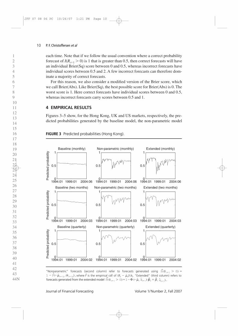
Figures 3–5 show, for the Hong Kong, UK and US markets, respectively, the pre-dicted probabilities generated by the baseline model, the non-parametric model

1234567891011121314151617181920212223242526272829303132333435363738394041424344N



FIGURE 3 Predicted probabilities (Hong Kong).

1994:01 1999:01 2004:060

0.5

1Baseline (monthly)

Pre

dict

ed p

roba

bilit

y

1994:01 1999:01 2004:060

0.5

1Non-parametric (monthly)

1994:01 1999:01 2004:060

0.5

1Extended (monthly)

Baseline (two months) Non-parametric (two months) Extended (two months)

Baseline (quarterly) Non-parametric (quarterly) Extended (quarterly)

1994:01 1999:01 2004:030

0.5

1

Pre

dict

ed p

roba

bilit

y

1994:01 1999:01 2004:030

0.5

1

1994:01 1999:01 2004:030

0.5

1

1994:01 1999:01 2004:020

0.5

1

Pre

dict

ed p

roba

bilit

y

1994:01 1999:01 2004:020

0.5

1

1994:01 1999:01 2004:020

0.5

1

forecasts generated from the extended model P̂r(Rt�1 � 0)�1��(��̂t x̂t�1)(̂�0 � �̂1 x̂t�1).where F̂ is the empirical cdf of (Rt � �̂t)/ �̂t. “Extended” (third column) refers to1 � F̂(��̂t�1�t/�̂t�1�t),

“Nonparametric” forecasts (second column) refer to forecasts generated using P̂r(Rt�1 � 0) �

JFF 07 08 06 PC 10/26/07 1:21 PM

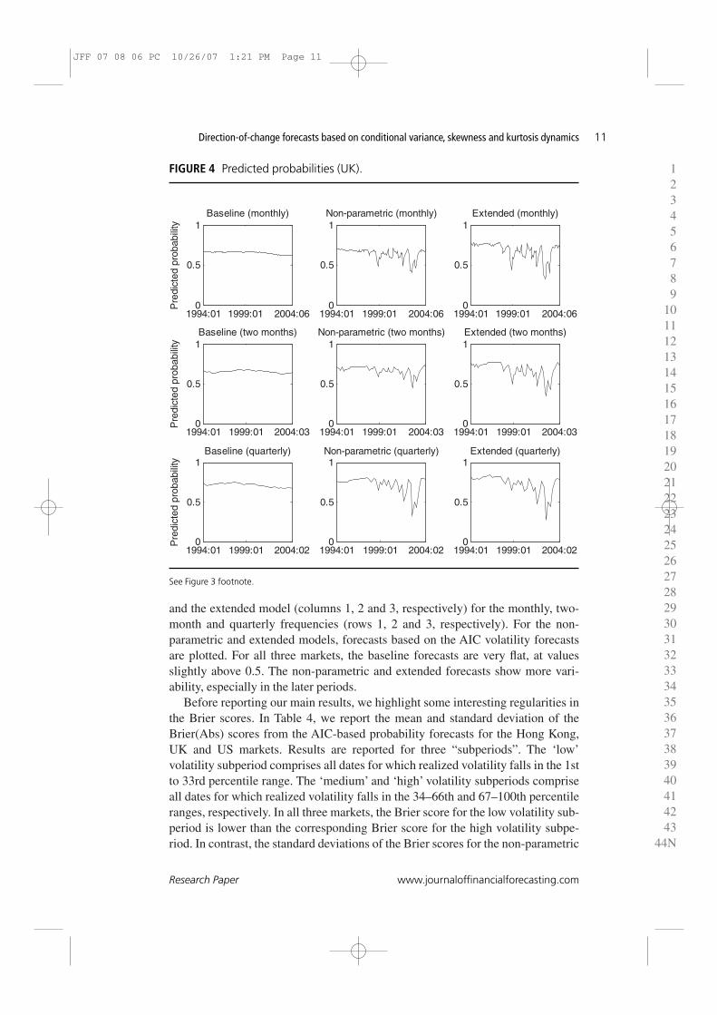
and the extended model (columns 1, 2 and 3, respectively) for the monthly, two-month and quarterly frequencies (rows 1, 2 and 3, respectively). For the non-parametric and extended models, forecasts based on the AIC volatility forecastsare plotted. For all three markets, the baseline forecasts are very flat, at valuesslightly above 0.5. The non-parametric and extended forecasts show more vari-ability, especially in the later periods.

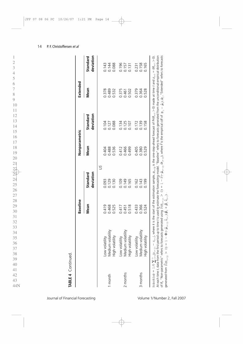
Before reporting our main results, we highlight some interesting regularities inthe Brier scores. In Table 4, we report the mean and standard deviation of theBrier(Abs) scores from the AIC-based probability forecasts for the Hong Kong,UK and US markets. Results are reported for three “subperiods”. The ‘low’volatility subperiod comprises all dates for which realized volatility falls in the 1stto 33rd percentile range. The ‘medium’ and ‘high’ volatility subperiods compriseall dates for which realized volatility falls in the 34–66th and 67–100th percentileranges, respectively. In all three markets, the Brier score for the low volatility sub-period is lower than the corresponding Brier score for the high volatility subpe-riod. In contrast, the standard deviations of the Brier scores for the non-parametric

123456789

10111213141516171819202122232425262728293031323334353637383940414243

44N



11

FIGURE 4 Predicted probabilities (UK).

1994:01 1999:01 2004:060

0.5

1

1994:01 1999:01 2004:060

0.5

1

1994:01 1999:01 2004:060

0.5

1

1994:01 1999:01 2004:030

0.5

1

1994:01 1999:01 2004:030

0.5

1

1994:01 1999:01 2004:030

0.5

1

1994:01 1999:01 2004:020

0.5

1

1994:01 1999:01 2004:020

0.5

1

1994:01 1999:01 2004:020

0.5

1

Baseline (monthly)

Pre

dict

ed p

roba

bilit

y

Non-parametric (monthly) Extended (monthly)



Pre

dict

ed p

roba

bilit

yP

redi

cted

pro

babi

lity

See Figure 3 footnote.

JFF 07 08 06 PC 10/26/07 1:21 PM

and extended models are higher in the low volatility subperiods than in the highvolatility subperiods. For instance, the mean Brier score for the extended model inthe US market at the monthly frequency is 0.378 in the low volatility subperiodand 0.532 in the high volatility subperiod. The standard deviation of the sameBrier scores falls from 0.143 in the low volatility subperiod to 0.088 in the highvolatility subperiod. These findings seem perfectly reasonable: we should expectour models to have more to say in subperiods of low volatility and little to say insubperiods of high volatility. In high volatility subperiods, the models tend to gen-erate probability forecasts that are close to 0.5. The corresponding Brier scores inturn tend to be close to 0.5, resulting in the lower standard deviation of Brierscores in high volatility subperiods.

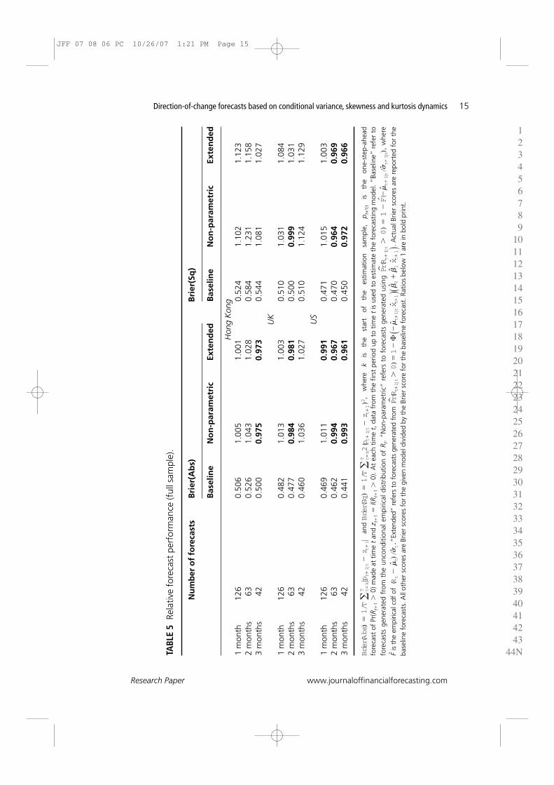
Our main results are reported in Tables 5–8. Table 5 contains our results forthe full forecast period. Tables 6–8 contain the results for the low, mediumand high volatility subperiods, respectively. In all four tables, both Brier(Abs)and Brier(Sq) are given for the baseline model. The Brier scores for the non-parametric and extended models are expressed relative to the baseline Brier

1234567891011121314151617181920212223242526272829303132333435363738394041424344N



FIGURE 5 Predicted probabilities (US).

1994:01 1999:01 2004:060

0.5

1

1994:01 1999:01 2004:060

0.5

1

1994:01 1999:01 2004:060

0.5

1

1994:01 1999:01 2004:030

0.5

1

1994:01 1999:01 2004:030

0.5

1

1994:01 1999:01 2004:030

0.5

1

1994:01 1999:01 2004:020

0.5

1

1994:01 1999:01 2004:020

0.5

1

1994:01 1999:01 2004:020

0.5

1

Baseline (monthly)

Pre

dict

ed p

roba

bilit

y

Non-parametric (monthly) Extended (monthly)



Pre

dict

ed p

roba

bilit

yP

redi

cted

pro

babi

lity

See Figure 3 footnote.

JFF 07 08 06 PC 10/26/07 1:21 PM

123456789

10111213141516171819202122232425262728293031323334353637383940414243

44N



13

TABL

E 4

Fore

cast

per

form

ance

, Brie

r(A

bs),

thre

e m

arke

ts.

Bas

elin

eN

on

par

amet

ric

Exte

nd

ed

Mea

nSt

and

ard

Mea

nSt

and

ard

Mea

nSt

and

ard

dev

iati

on

dev

iati

on

dev

iati

on

Hon

g K

ong

Low

vol

atili

ty0.

507

0.07

50.

510

0.20

80.

504

0.23

91

mon

thM

ediu

m v

olat

ility

0.49

10.

070

0.47

50.

168

0.47

50.

182

Hig

h vo

latil

ity0.

520

0.07

60.

537

0.13

70.

535

0.15

1

Low

vol

atili

ty0.

512

0.12

60.

518

0.29

80.

512

0.26

52

mon

ths

Med

ium

vol

atili

ty0.

487

0.12

10.

487

0.23

00.

488

0.20

3H

igh

vola

tility

0.57

90.

107

0.64

00.

173

0.62

20.

145

Low

vol

atili

ty0.

435

0.13

20.

390

0.24

10.

402

0.22

33

mon

ths

Med

ium

vol

atili

ty0.

515

0.14

40.

526

0.25

60.

524

0.22

2H

igh

vola

tility

0.55

10.

154

0.54

80.

202

0.53

40.

159

UK

Low

vol

atili

ty0.

430

0.13

70.

418

0.16

40.

388

0.22

41

mon

thM

ediu

m v

olat

ility

0.50

70.

157

0.51

60.

165

0.51

90.

215

Hig

h vo

latil

ity0.

500

0.15

10.

522

0.12

30.

531

0.15

3

Low

vol

atili

ty0.

398

0.10

60.

362

0.14

70.

333

0.18

12

mon

ths

Med

ium

vol

atili

ty0.

511

0.16

00.

526

0.17

80.

546

0.19

3H

igh

vola

tility

0.51

70.

160

0.51

40.

154

0.51

80.

158

Low

vol

atili

ty0.

343

0.15

60.

308

0.20

40.

288

0.22

63

mon

ths

Med

ium

vol

atili

ty0.

470

0.22

00.

484

0.24

70.

491

0.25

4H

igh

vola

tility

0.56

60.

201

0.63

80.

173

0.63

80.

162

JFF 07 08 06 PC 10/26/07 1:21 PM

1234567891011121314151617181920212223242526272829303132333435363738394041424344N



TABL

E 4

Con

tinue

d.

Bas

elin

eN

on

par

amet

ric

Exte

nd

ed

Mea

nSt

and

ard

Mea

nSt

and

ard

Mea

nSt

and

ard

dev

iati

on

dev

iati

on

dev

iati

on

US

Low

vol

atili

ty0.

419

0.09

30.

404

0.10

40.

378

0.14

31

mon

thM

ediu

m v

olat

ility

0.46

80.

129

0.48

80.

127

0.48

90.

144

Hig

h vo

latil

ity0.

525

0.13

00.

536

0.08

80.

532

0.08

8

Low

vol

atili

ty0.

417

0.10

90.

412

0.13

40.

375

0.19

62

mon

ths

Med

ium

vol

atili

ty0.

451

0.14

90.

466

0.12

50.

461

0.15

7H

igh

vola

tility

0.51

80.

165

0.49

90.

107

0.50

20.

131

Low

vol

atili

ty0.

433

0.16

20.

405

0.17

20.

379

0.23

13

mon

ths

Med

ium

vol

atili

ty0.

366

0.14

30.

380

0.13

90.

364

0.15

8H

igh

vola

tility

0.52

40.

199

0.52

90.

158

0.52

80.

165

, w

here

kis

the

sta

rt o

f th

e es

timat

ion

sam

ple,

pt�

1�tis

the

one

-ste

p-ah

ead

fore

cast

of

Pr(R

t�1

�0)

mad

e at

tim

e t

and

z t�

1�

I(R t

�1

�0)

.Brier(Abs)

�1/T �

t�k

T�pt�

1�t

�z t

�1�

At e

ach

time

t, d

ata

from

the

first

per

iod

up to

tim

e ti

s us

ed to

est

imat

e th

e fo

reca

stin

g m

odel

. “Ba

selin

e” re

fers

to fo

reca

sts

gene

rate

d fr

om th

e un

cond

ition

al e

mpi

rical

dis

trib

utio

nof

Rt.

“Non

-par

amet

ric”

refe

rs t

o fo

reca

sts

gene

rate

d us

ing

, whe

re F̂

is t

he e

mpi

rical

cdf

of

“Ext

ende

d” re

fers

to

fore

cast

s(R

t�

�̂t)/�̂

t.P̂r(R

t�1

�t�

0)

�1

�F̂(

��̂t�

1�t/�̂

t�1

�t)ge

nera

ted

from

.P̂r(R

t�1

�t�

0)

�1

��(�

�̂t�

1�tx̂ t

�1)(̂

�0

��̂1x̂ t

�1)

JFF 07 08 06 PC 10/26/07 1:21 PM

123456789

10111213141516171819202122232425262728293031323334353637383940414243

44N



15

TABL

E 5

Rela

tive

fore

cast

per

form

ance

(ful

l sam

ple)

.

Nu

mb

er o

f fo

reca

sts

Bri

er(A

bs)

Bri

er(S

q)

Bas

elin

eN

on

-par

amet

ric

Exte

nd

edB

asel

ine

No

n-p

aram

etri

cEx

ten

ded

Hon

g K

ong

1 m

onth

126

0.50

61.

005

1.00

10.

524

1.10

21.

123

2 m

onth

s63

0.52

61.

043

1.02

80.

584

1.23

11.

158

3 m

onth

s42

0.50

00.

975

0.97

30.

544

1.08

11.

027

UK

1 m

onth

126

0.48

21.

013

1.00

30.

510

1.03

11.

084

2 m

onth

s63

0.47

70.

984

0.98

10.

500

0.99

91.

031

3 m

onth

s42

0.46

01.

036

1.02

70.

510

1.12

41.

129

US

1 m

onth

126

0.46

91.

011

0.99

10.

471

1.01

51.

003

2 m

onth

s63

0.46

20.

994

0.96

70.

470

0.96

40.

969

3 m

onth

s42

0.44

10.

993

0.96

10.

450

0.97

20.

966

fore

cast

of

Pr(R

t�1

�0)

mad

e at

tim

e t

and

z t�

1�

I(Rt�

1�

0). A

t ea

ch t

ime

t, d

ata

from

the

firs

t pe

riod

up t

o tim

e t

is u

sed

to e

stim

ate

the

fore

cast

ing

mod

el. “

Base

line”

ref

er t

o

base

line

fore

cast

s. A

ll ot

her

scor

es a

re B

rier

scor

es f

or t

he g

iven

mod

el d

ivid

ed b

y th

e Br

ier

scor

e fo

r th

e ba

selin

e fo

reca

st. R

atio

s be

low

1 a

re in

bol

d pr

int.

fore

cast

s ge

nera

ted

from

the

unc

ondi

tiona

l em

piric

al d

istr

ibut

ion

of R

t. “N

on-p

aram

etric

” re

fers

to

fore

cast

s ge

nera

ted

usin

g ,

whe

re

P̂r(R

t�1

�t�

0)

�1

�F̂(

��̂t�

1�t/�̂

t�1

�t)F̂

is t

he e

mpi

rical

cdf

of

“Ext

ende

d” re

fers

to

fore

cast

s ge

nera

ted

from

. A

ctua

l Brie

r sc

ores

are

rep

orte

d fo

r th

eP̂r(R

t�1

�t�0

)�1

��

��̂t�1

�tx̂ t

�1

��̂0

��̂1x̂ t

�1

�(R

t�

�̂t)/�̂

t.

and

, w

here

k

is

the

star

t of

th

e es

timat

ion

sam

ple,

p t

+1�

tis

th

e on

e-st

ep-a

head

Brier(Sq

)�1/T �

t�k

T2(p

t�1

�t�z t

�1)2

Brier(Abs)

�1/T �

t�k

T�pt�

1�t

�z t

�1�

JFF 07 08 06 PC 10/26/07 1:21 PM

1234567891011121314151617181920212223242526272829303132333435363738394041424344N



TABL

E 6

Fore

cast

per

form

ance

, low

vol

atili

ty p

erio

ds (1

st t

o 33

rd p

erce

ntile

).

Nu

mb

er o

f fo

reca

sts

Bri

er(A

bs)

Bri

er(S

q)

Bas

elin

eN

on

-par

amet

ric

Exte

nd

edB

asel

ine

No

n-p

aram

etri

cEx

ten

ded

Hon

g K

ong

1 m

onth

420.

507

1.00

40.

993

0.52

61.

148

1.17

82

mon

ths

210.

512

1.01

11.

000

0.55

51.

269

1.18

63

mon

ths

140.

435

0.89

60.

923

0.41

11.

002

1.01

0U

K1

mon

th42

0.43

00.

972

0.90

40.

406

0.99

00.

985

2 m

onth

s21

0.39

80.

909

0.83

60.

338

0.89

60.

839

3 m

onth

s14

0.34

30.

897

0.83

90.

281

0.95

00.

929

US

1 m

onth

420.

419

0.96

40.

903

0.36

80.

944

0.88

72

mon

ths

210.

417

0.98

90.

899

0.37

01.

011

0.95

63

mon

ths

140.

433

0.93

40.

875

0.42

30.

902

0.91

1

See

Tabl

e 5

foot

note

.

JFF 07 08 06 PC 10/26/07 1:21 PM

123456789

10111213141516171819202122232425262728293031323334353637383940414243

44N



17

TABL

E 7

Fore

cast

per

form

ance

, med

ium

vol

atili

ty p

erio

ds (3

4–66

th p

erce

ntile

).

Nu

mb

er o

f fo

reca

sts

Bri

er(A

bs)

Bri

er(S

q)

Bas

elin

eN

on

-par

amet

ric

Exte

nd

edB

asel

ine

No

n-p

aram

etri

cEx

ten

ded

Hon

g K

ong

1 m

onth

420.

491

0.96

70.

966

0.49

21.

029

1.04

62

mon

ths

210.

487

1.00

01.

002

0.50

21.

144

1.10

43

mon

ths

140.

515

1.02

21.

019

0.56

81.

187

1.12

9U

K1

mon

th42

0.50

71.

017

1.02

30.

563

1.04

01.

116

2 m

onth

s21

0.51

11.

028

1.06

80.

572

1.07

21.

168

3 m

onth

s14

0.47

01.

029

1.04

50.

532

1.09

31.

133

US

1 m

onth

420.

468

1.04

31.

047

0.47

01.

080

1.10

62

mon

ths

210.

451

1.03

21.

023

0.44

91.

031

1.05

23

mon

ths

140.

366

1.04

00.

996

0.30

61.

065

1.02

1

See

Tabl

e 5

foot

note

.

JFF 07 08 06 PC 10/26/07 1:21 PM

1234567891011121314151617181920212223242526272829303132333435363738394041424344N



TABL

E 8

Fore

cast

per

form

ance

, hig

h vo

latil

ity p

erio

ds (6

6th–

100t

h pe

rcen

tile)

.

Nu

mb

er o

f fo

reca

sts

Bri

er(A

bs)

Bri

er(S

q)

Bas

elin

eN

on

-par

amet

ric

Exte

nd

edB

asel

ine

No

n-p

aram

etri

cEx

ten

ded

Hon

g K

ong

1 m

onth

420.

520

1.03

21.

029

0.55

21.

110

1.11

82

mon

ths

210.

579

1.10

51.

075

0.69

21.

265

1.17

63

mon

ths

140.

551

0.99

50.

970

0.65

21.

040

0.94

9U

K1

mon

th42

0.50

01.

044

1.06

30.

544

1.05

31.

121

2 m

onth

s21

0.51

70.

995

1.00

20.

583

0.98

41.

002

3 m

onth

s14

0.56

61.

127

1.12

60.

717

1.21

41.

204

US

1 m

onth

420.

525

1.02

11.

015

0.58

31.

009

0.99

72

mon

ths

210.

518

0.96

40.

969

0.58

80.

885

0.91

23

mon

ths

140.

524

1.00

91.

008

0.62

20.

974

0.97

7

See

Tabl

e 5

foot

note

.

JFF 07 08 06 PC 10/26/07 1:21 PM

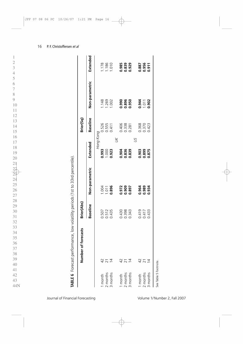
scores. A relative measure of less than 1 therefore implies improvement in fore-cast performance.

Table 5 reports improvement in the performance of the non-parametric orextended models over the baseline forecasts in half of the cases considered, whenusing Brier(Abs) as a measure of performance. All of the improvements, however,are very small. The situation is usually worse when the forecasts are evaluatedusing Brier(Sq) instead.

The fact that the non-parametric and extended models perform better duringlow volatility subperiods than during high volatility subperiods suggests that theirperformance relative to the baseline model might be better during low volatilitysubperiods than during high volatility subperiods. This is verified by the relativeperformances reported in Tables 6–8. In Table 6, the improvements are wide-spread and sometimes large. In a number of cases, the ratio of the Brier(Abs)scores for the extended/parametric models to the baseline model is less than 0.9.

123456789

10111213141516171819202122232425262728293031323334353637383940414243

44N



19

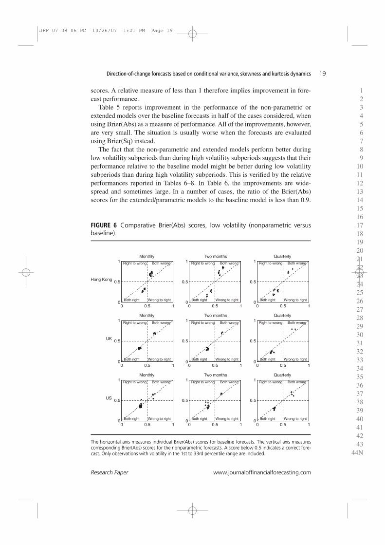
FIGURE 6 Comparative Brier(Abs) scores, low volatility (nonparametric versusbaseline).

0 0.5 10

0.5

1

Hong Kong

Monthly

Right to wrong

Both right

Both wrong Right to wrong Both wrong Right to wrong Both wrong

Wrong to right Both right Wrong to right Both right Wrong to right

Right to wrong

Both right



Right to wrong

Both right



0 0.5 10

0.5

1Two months

0 0.5 10

0.5

1Quarterly

0 0.5 10

0.5

1

UK

Monthly

0 0.5 10

0.5

1Two months

0 0.5 10

0.5

1Quarterly

0 0.5 10

0.5

1

US

Monthly

0 0.5 10

0.5

1Two months

0 0.5 10

0.5

1Quarterly

The horizontal axis measures individual Brier(Abs) scores for baseline forecasts. The vertical axis measurescorresponding Brier(Abs) scores for the nonparametric forecasts. A score below 0.5 indicates a correct fore-cast. Only observations with volatility in the 1st to 33rd percentile range are included.

JFF 07 08 06 PC 10/26/07 1:21 PM

When Brier(Sq) is used to measure forecast performance, there are fewerinstances where the non-parametric and extended models perform better than thebaseline. The notable differences between the Brier(Sq) scores and Brier(Abs)scores occur for Hong Kong, where Brier(Sq) shows no improvements from thenon-parametric and extended models.

The ratios under Brier(Abs) also show that the extended model performs muchbetter than the non-parametric model. We note also that for both Brier(Abs) andBrier(Sq), the performance of the non-parametric and extended models, relative tothe baseline, is generally better at the quarterly frequency than at the monthly fre-quency. This is to be expected, as the theory indicates that volatility-aided predic-tion depends on a sizable mean return, and the mean return increases in allmarkets as we go from monthly to quarterly frequencies.

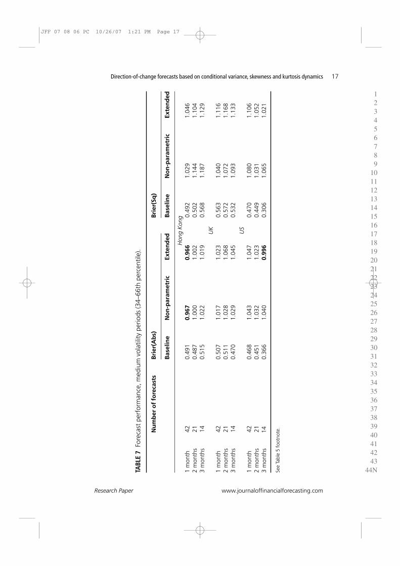
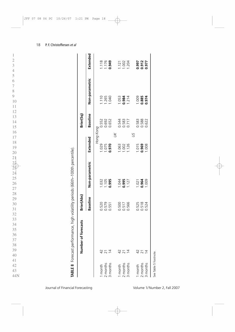
In the medium and high volatility subperiods in Tables 7 and 8, respectively,much less improvement in the performance of the non-parametric and extended

1234567891011121314151617181920212223242526272829303132333435363738394041424344N



FIGURE 7 Comparative Brier(Abs) scores, low volatility (extended model versusbaseline).

0 0.5 10

0.5

1

Hong Kong

Monthly

Right to wrong

Both right

Both wrong

Wrong to right

Right to wrong

Both right

Both wrong

Wrong to right

0 0.5 10

0.5

1Two months

0 0.5 10

0.5

1Quarterly

0 0.5 10

0.5

1

UK

Monthly

0 0.5 10

0.5

1Two months

0 0.5 10

0.5

1Quarterly

0 0.5 10

0.5

1

US

Monthly

0 0.5 10

0.5

1Two months

0 0.5 10

0.5

1Quarterly

Right to wrong

Both right

Both wrong

Wrong to right

Right to wrong

Both right

Both wrong

Wrong to right

Right to wrong

Both right

Both wrong

Wrong to right

Right to wrong

Both right

Both wrong

Wrong to right

Right to wrong

Both right

Both wrong

Wrong to right

Right to wrong

Both right

Both wrong

Wrong to right

Right to wrong

Both right

Both wrong

Wrong to right

The horizontal axis measures individual Brier(Abs) scores for baseline forecasts. The vertical axis measurescorresponding Brier(Abs) scores for the extended forecasts. A score below 0.5 indicates a correct forecast.Only observations with volatility in the 1st to 33rd percentile range are included.

JFF 07 08 06 PC 10/26/07 1:21 PM

models is found. It appears that volatility in these subperiods is simply too largerelative to the mean to be useful in guiding direction-of-change forecasts.

Figures 6 and 7 show a clear picture of the forecast performance of the non-parametric and extended models compared to the baseline forecasts. At each fre-quency, we show a scatterplot of the Brier(Abs) scores of individual forecasts.We include only observations when volatility is low, as previously defined. In bothfigures, the horizontal axis measures the Brier(Abs) scores for individual baselineforecasts. In Figure 6, the vertical axis measures the Brier(Abs) scores forindividual non-parametric forecasts. In Figure 7, the vertical axis measures theBrier(Abs) scores for individual forecasts from the extended model. In addition tothe scatterplots, we include a horizontal and vertical gridline at 0.5 and a 45° line.As a Brier(Abs) score below 0.5 indicates a correct forecast, points in the lowerleft quadrant indicate that both competing forecasts are correct, whereas a point inthe lower right quadrant indicates that the baseline forecast for this observation isincorrect, with the competing forecast correct. Points below the 45° line indicateimprovements in the Brier(Abs) scores over the baseline.

In all three markets, the non-parametric and extended models clearly providebetter signals than the baseline model when both the baseline and the competingforecasts are correct. However, for Hong Kong and UK, the performance of thenon-parametric and extended model is worse than the baseline model when thebaseline and the competing forecasts are wrong. Note that the upper left and lowerright quadrants of Figures 6 and 7 are mostly empty, which implies that the mod-els by and large make predictions that are similar to the baseline forecasts.Nonetheless, there is evidence that when volatility is low, forecasts of volatilitycan improve the quality of the signal, in the sense of providing probability fore-casts with improved Brier scores.

5 SUMMARY AND DIRECTIONS FOR FUTURE RESEARCH

Methodologically, we have extended the Christoffersen and Diebold (2006)direction-of-change forecasting framework to include the potentially importanteffects of higher-ordered conditional moments. Empirically, in an application to asample of three equity markets, we have verified the importance of allowingfor higher-ordered conditional moments and taken a step toward evaluating thereal-time predictive performance. In future work, we look forward to using ourdirection-of-change forecasts to formulate and evaluate actual trading strategiesand to exploring their relationships to the “volatility timing” strategies recentlystudied by Fleming et al (2003), in which portfolio shares are dynamicallyadjusted based on forecasts of the variance–covariance matrix of the underlyingassets.

REFERENCES

Andersen, T. G., Bollerslev, T., Diebold, F. X., and Labys, P. (2003). Modeling and forecast-ing realized volatility. Econometrica 71, 579–626.

123456789

10111213141516171819202122232425262728293031323334353637383940414243

44N



21

JFF 07 08 06 PC 10/26/07 1:21 PM

Andersen, T. G., Bollerslev, T., Christoffersen, P. F., and Diebold, F. X. (2006). Volatility andcorrelation forecasting. Handbook of Economic Forecasting, Elliott, G., Granger, C. W. J.and Timmermann, A. (eds). North-Holland, Amsterdam 777–878.

Brandt, M. W., and Kang, Q. (2004). On the relationship between the conditional meanand volatility of stock returns: a latent VAR approach. Journal of Financial Economics72, 217–257.

Christoffersen, P. F., and Diebold, F. X. (2006). Financial asset returns, direction-of-changeforecasting, and volatility dynamics. Management Science 52, 1273–1287.

Diebold, F. X. and Lopez, J. (1996). Forecast evaluation and combination. Handbookof Statistics, Maddala, G. S. and Rao, C. R. (eds). North-Holland, Amsterdam, pp. 241–268.

Engle, R. F., Lilien, D. M., and Robins, R. P. (1987). Estimating time varying risk premia inthe term structure: the Arch-M model. Econometrica 55, 391–407.

Fleming, J., Kirby, C., and Ostdiek, B. (2003). The economic value of volatility timing usingrealized volatility. Journal of Financial Economics 67, 473–509.

Lettau, M., and Ludvigson, S. (2005). Measuring and modeling variation in the risk-returntradeoff. Handbook of Financial Econometrics, Ait-Shalia, Y. and Hansen, L. P. (eds).North-Holland, Amsterdam, forthcoming.

1234567891011121314151617181920212223242526272829303132333435363738394041424344N



JFF 07 08 06 PC 10/26/07 1:21 PM

Direction-of-change forecasts based on conditional ...fdiebold/papers/paper73/CDMTT.pdf · Roberto...

Documents

Transcript of Direction-of-change forecasts based on conditional ...fdiebold/papers/paper73/CDMTT.pdf · Roberto...