Direct Solution of the Vorticity-stream Function Ordinary Differential Equations by a Chebyshev...

JOURNAL OF COMPUTATIONAL PHYSICS 52, 448-463 (1983)

Direct Solution of the Vorticity-Stream Function Ordinary Differential Equations by a Chebyshev Approximation

S. C. R. DENNIS

Department @Applied Mathematics, University of Western Ontario, London, Ontario, Canada

AND

L. QUARTAPELLE

Istituto di Fisica, Politecnico di Milano, Milan, Italy

Received August 24, 1982; revised January 19, 1983

A numerical method for solving the coupled vorticity-stream function equations in one dimension with an exact noniterative determination of the vorticity boundary values is presented. The one-dimensional form considered can represent the Fourier modes of a two- dimensional problem. The equations are separated by replacing the derivative specifications for the stream function at the boundary points with equivalent conditions of an integral type for the vorticity. A spectral approximation by means of Chebyshev polynomials is considered. The numerical properties of the algorithm are investigated against a few analytical examples which demonstrate the accuracy of the proposed method.

1. INTRODUCTION

The method of the truncated series expansion in orthogonal functions [ I ] has been widely used to obtain approximate solutions of the Navier-Stokes equations for viscous incompressible flows. The presence of no-slip boundary conditions, however, causes special difficulties which have limited so far the applications of Galerkin and collocation methods mainly to problems belonging to the following classes: turbulent flows with periodic boundary conditions [2-41; plane or axisymmetric flows in which no-slip conditions are prescribed only on two opposite sides of the computational domain [5-g]; and three-dimensional flows in plane channels with periodic conditions in directions parallel to the planes and no-slip conditions on the planes [ 10-131.

In the case of the vorticity-stream function equations, the no-slip conditions are troublesome since they imply the boundary specification of both the stream function and its normal derivative but none for the vorticity. The expansion method is thus employed to represent the dependence on only one spatial variable, whereas finite differences are typically used to discretize the spatial variable involved by the no-slip

448 0021.9991183 $3.00 Copyright 0 1983 by Academic Press. Inc. All rights of reproduction in any form reserved.

SPECTRAL VORTICITY CONDITIONS 449

boundary conditions [5-91. On the other hand, a formulation of the continuum problem is possible in which the above difficulty is circumvented by introducing conditions of an integral character for the vorticity. Conditions of this type have been successfully employed in one-dimensional form using finite differences (see, e.g., [9] and the references therein) and in two-dimensional form using both finite differences [ 141 and finite elements [ 151. Since expansion or spectral methods provide approximations of a global character, the use of exact integral conditions for the vorticity is expected to be especially appropriate for discretization methods of this type. It seems therefore worthwhile to investigate the applicability of the integral conditions to the spectral solution of the vorticity-stream function equations. Before addressing the fully two-dimensional equations with no-slip conditions prescribed on the entire boundary, it seems also convenient to consider the case of one-dimensional equations such as those governing the vorticity and stream function coefficients of a Fourier mode of a problem in two dimensions. In this note a direct (noniterative) algorithm is described for solving Chebyshev approximation to the pair of ordinary differential equations of this type which are coupled together by the double specification on the stream function. By virtue of the (one-dimensional) integral conditions for the vorticity, the equations typical of stationary or evolution problems are written in a factorized form. Two methods for computing the relevant quantities allowing such a splitting are considered: the first method is an adaptation to the present case of the formulation proposed by Glowinski and Pironneau for the bihar- manic problem in two dimensions [ 161; the second approach is based on the influence matrix method employed by Kleiser and Schumann in the calculation of three-dimensional plane channel flows by means of the primitive variables [ 12, 131. The problem of evaluating integrals of threefold products of Chebyshev polynomials is also considered. The integrals provide the interaction coefficients which are required in the iterative solution of the nonlinear Navier-Stokes equations by means of the proposed algorithm.

2. BASIC EQUATIONS

Let us consider the linear system of two second-order ordinary differential equations

(2.1)

Dyl= EC, (2.2)

where c and w are the unknown variables, y is a constant, E = E(X) and u = c(x) are given functions defined on the integration interval [x, , x,]. In Eqs. (2.1~(2.2) D is a second-order differential operator defined by

Lb=--~“+up’+v~,, (2.3)

450 DENNIS AND QUARTAPELLE

where u and u are given constants and the prime denotes the derivative with respect to x. Equations of this type are encountered when the method of series expansions is employed in the solution of the Navier-Stokes equations for plane or axymmetric viscous flows in terms of the vorticity and stream function variables [ 1). The dependence on one of the two spatial variables is represented by a truncated series of suitable orthogonal polynomials and a nonlinear system of coupled differential equations is obtained for the expansion coefficients which depend on the second spatial variable. In the case of stationary problems the equations are ordinary differential equations, whereas in time-dependent problems a system of partial differential equations with two independent variables is obtained. The latter, after the equations are discretized in time by finite differences, gives rise to a system of ordinary differential equations at each time level. In both cases, the solution of the resulting nonlinear system can be calculated iteratively by solving a finite number of pairs of linear second-order differential equations for the coefficients < and v in the series expansions of the vorticity and stream functions fields. The equations to be solved have the form given in Eqs. (2.1)-(2.3) with possibly additional nonconstant- coefficient terms in Eq. (2.1) coming from the nonlinear part of the vorticity transport equation (see Section 7.2). In stationary problems y = 0, whereas in transient problems, typically, y = Re/dt. Furthermore, using Cartesian coordinates E(X) = 1, whereas using a stretched radial variable for cylindrical or spherical domains E(X) = ezx.

As far as the conditions for these equations are concerned, the prescription of both components of the velocity at the boundary originates specifications for both the stream function and its derivative at xi and x2, so that Eqs. (2.1~(2.2) are typically supplemented by the boundary conditions

v4x,> = a,, I= 1, 2, (2.4)

v’(x,> = b, 3 I= 1,2, (2.5)

where a, and b,, I = 1,2, are specified from the normal and tangential components of the velocity on the boundary.

3. SPLITTING OF THE EQUATIONS

The simultaneous specification of IJ and w’ at each boundary point introduces a coupling betyeen the linear equations (2.1) and (2.2) for [ and t,u, respectively. It is possible, however, to obtain two independent conditions for the vorticity, and henceforth a complete splitting of the equations, by means of the simple Green’s identity in one dimension given by


Here Dt is the operator adjoint to D defined by Eq. (2.3), namely,

D+rpr-rp”-uqf+vcp. (3.2)

Notice that D is self-adjoint if and only if u = 0. From Green’s identity (3.1) it follows that EC = DI,u, with I = a, and @(xl) = b,, if and only if C satisfies the two integral conditions

i x2 @q, dx = -[bv, - a(~; + uy,)];: = c/, (3.3) x1

where q,, I = 1, 2, are such that

D+q,=O, ?,t4 = 4,7 m= 1,2. (3.4)

In Eq. (3.3) b = b(x,) E b, and a = a(~,) = a,; furthermore, in Eq. (3.4) a,,,, is the Kronecker delta. The problem given by Eqs. (2.1)-(2.4) can be restated as a system of two split ordinary differential equations

DC + y&C = o, I

x2 4v, dx = c/, I= 1,2; (3.5)

XI

Dv = 4, v(x,) = a, 3 1= 1,2. (3.6)

Each is supplemented by its own conditions, the former by integral conditions and the latter by conditions of the usual boundary-value type.

If the vorticity or its derivative is specified at one of the end points, say x, , there is only one integral condition on 4. In this case, the function q to be used in the integral condition satisfies the same equation and the same condition at xz valid for the function q2, namely,

D+q=O, ?(Xz) = 1. (3.7)

As far as the condition at x, is concerned, we have

r(x,)=O or v’tx,) + U?(X,> = 0 (3.7’)

according to whether the boundary condition specified at x, for w is I&,) or I$(x,), respectively.

4. DECOMPOSITION SCHEME FOR THE INTEGRALLY CONDITIONED VORTICITY

EQUATION

To simplify the notation, let us introduce the linear operator E = E(x) G D + y&(x) so that the vorticity equation (3.5) can be rewritten in the form

EC = u, 5

X2 @,I, dx = c,. (4.1) XI


Henceforth we will omit the specification I = 1, 2 for simplicity. The solution of the integrally conditioned vorticity equation (4.1) can be expressed in the form

C=Co+a,L+a2L, (4.2)

where &,,, m = 1, 2, and [,, are the solutions of the problems

EC,,, = 0, L(x,) = 4d 3 (4.3)

and

respectively. Thus a1 and a2 are the values of the vorticity at the end points x1 and x2. By imposing that [ satisfies the integral conditions, we find that the two- component vector a - {a,, a?} is the solution of the linear system

Au=&

where the matrix A and the vector B are defined by the relationships

(4.5)

A [,,, = I x2 4, ‘I/ dx, Xl

I,m= 1,2, (4.6)

P, = - jx2 4,j 9, dx + c/r XI

I= 1,2. (4.7)

By virtue of Green’s identity (3.1), matrix A is symmetric if and only if u = 0, i.e., if and only if D is self-adjoint. In the case u = u = 0 the present formulation becomes the one-dimensional equivalent of the split formulation for the biharmonic equation [141*

5. GLOWINSKI-PIRONNEAU METHOD

The problem defined by Eqs. (2.1)-(2.2) supplemented and coupled by conditions (2.4~(2.5) has been transformed into a cascade of independent problems (4.3), (4.4), (4.5), and (3.6) to be solved in sequence. However, instead of evaluating A and p directly through Eqs. (4.6) and (4.7), it is computationally more convenient to resort to a different characterization of these quantities which does not require to calculate the functions ‘I,. Such a method results from adapting the general formulation proposed by Glowinski and Pironneau for the direct solution of the biharmonic equation [ 161 to the present case of nonsymmetric one-dimensional equations. In place of the functions r,,,, m = 1, 2, solutions of problem (3.4), one introduces the functions W, = w,(x), m =. 1,2, defined such that

w,,,(x) = arbitrary, x, <X(X2, ~A-%) = 4d. (5.1)


Then A is calculated from the functions [,,, and lm, m = 1, 2, which are the solutions of the equations

EC, = 0, Ln(xJ = 4n, 7 (5.2)

Dw,,, = d,,,, Wmc4 = 0. (5.3)

By virtue of Green’s identity (3.1$, it is possible to obtain from Eq. (4.6)

A,, = I 1; [M?l - w:, - w,)w - w:,w;1 dr*

Similarly, from Eq. (4.7), B can be obtained from

(5.4)

EL, = (J, Mx,) = 09 (5.5)

Dwo = 4o > w&J = a/ 3 (5.6)

p, = - jx2 [(&Co - uly; - uy/,)w, - l&w;] dx - [bw,]$ (5.7) XI

Once the vorticity boundary values a, and a, have been obtained from the linear system

Aa=p (5.8)

the solution of the original problem is obtained from the equations

E<=a, K%) = a/, (5.9)

Dv = 4, W(Xr> = a,. (5.10)

Notice that, by exploiting the arbitrariness of W, for x, < x < x2, the functions w,, m = 1, 2, can be generated whenever required and need not be stored.

6. INFLUENCE MATRIX METHOD

An alternative method for evaluating A and B is provided by the influence (or capacitance) matrix method, which has been employed by Kleiser and Schumann to solve the similar problem of missing boundary conditions for the pressure variable in incompressible flows [ 12-131. By exploiting the linearity of Eqs. (2.1)-(2.2), one can expand the solution ([, IJ/) in the form

(6.1)

where (Co, IJI,J and ([,, w,), m = 1, 2, are the solutions of problems (5.5~(5.6) and


(5.2)-(5.3), respectively. By imposing the satisfaction of the derivative boundary conditions #(x,) = b,, I = 1, 2, the linear system Aa = p for a F (a,, aI) is obtained where A and p are defined by

A,, = wL(xA (6.2)

P, = --wlxx,) + b, * (6.3)

These expressions are much simpler than the corresponding expressions of the Glowinski-Pironneau method but they require the evaluation of pointwise derivatives, and this operation can give rise to numerical inaccuracies.

7. CHEBYSHEV APPROXIMATION

7.1 Vorticity-Stream Function Equations

The typical c-w equations to be solved in the algorithm discussed so far are of the form

4” + 246’ + UC + y&c = c7, Ctx,) = 4,

-w” + uy’ + VW = El, w(x,> = aI.

(7.1)

(7.2)

Let us assume that x, = -1 and x2 = 1. We expand 4 and w in a truncated series of Chebyshev polynomials 7’,(x) = cos [n cos - l(x)] in the respective forms

and v/(x) = $ v, T”(X). n=O

(7.3)

The discrete form of the vorticity equations and boundary conditions (7.1) is provided by the tau method [ 17-181 expressed by

-p + up + I$, + y -f E,Jp = (Jn, O<n<N-2, (7.4a) p=o

,fo t-K, = 4 7 (7.4b)

where we use the notation qc’ for the coefficients of the ith derivative of a Chebyshev series p(x) with coefficients p,,. The matrix E,, in Eq. (7.4a) is defined by

(7.4c)


where c, = 2 and c, = 1, n > 1. Similarly, the tau approximation of problem (7.2) is

N

-y/(*’ + my(‘) + uy/ 7 r n ” ” L %PCP, O<n<N-2, (7.5a)

p=o (7Sb)

The linear system of the vorticity equations (7.4) has a matrix of coefficients which is full if y # 0. The matrix of the coefficients for the stream function equations (7.5) has always nonzero entries only in the upper triangle and in the two first lower codiagonals. Due to the presence of the coefficients of the first derivative this matrix cannot be transformed to a nearly pentadiagonal form by means of the Haidvogel algorithm [ 191.

7.2 Nonconstant Coeflcient Terms

In typical fluid dynamic applications, the vorticity equation (7.1) contains additional terms with nonconstant coefficients which originate from the nonlinearities of the vorticity transport equation. In such cases, the operator E of the vorticity equation is redefined as

a = P + Y&(X)] c + f(x) C’ + g(x) 5 t h’(x) (I, (7.6)

where f, g, and h are assumed to be known functions. If they are expanded in Chebyshev truncated series and their Chebyshev coefficients are known, the presence of the new terms can be taken into account by adding to the left-hand side of Eq. (7.4a) the quantity

-1 N

pzo CP qio (Lnq~fs + *mm g, + Lnpqhq),

where

*npq = I +’ T,(x) T,(x) T,(x) dx -1 (1 - x2)“*

(7.8)

and

L nP4 = I + ’ T,(x) T,(x) T;(x) dx

(1 -x*)v* * (7.9) -1

Using well-known results [ 17, p. 521, the integrals are found to be

*npq = wktfv”,P+q + 4,,P-,,I. (7.10)


As far as the integrals Lnp4 are concerned, by means of known results we find, in terms of the function U,(cos 19) = [sin(n + 1)8]/sin 0 [ 17, p. 531,

L 4 +’ u 6) np? = - 4 11 -1

q+P+.Ax) dx + j’,’ ~l+“-;*j~,* dx (1 -x2)“*

+’ u +

I q-p+n-1(x> dx + +I Uq-p-n-1(4 dx

-1 (1 -x2)“* !’ -1 (1 -x*)1’* 1 a (7.11)

The integrals on the right can be evaluated using the results

I +* U”(X) dx=O if n is odd (positive or negative), -, (1 -x2)“*

=7l if n is even and > 0, (7.12)

Z-n if n is even and < 0.

We notice that, when the nonconstant coefficient terms are present, &,,, m = 1, 2, and henceforth A depend on the functions f, g, and h.

The two linear systems for the vorticity, Eqs. (7.4) and (7.7), and for the stream function, Eqs. (7.5), are solved by the LU decomposition. In the case of the stream function equations the matrix has a nearly triangular profile, and therefore the algorithm is modified to avoid the calculation in the lower triangle, but for the first two lower codiagonals.

In truly nonlinear problems, a substantial gain in computational efficiency can be obtained by evaluating the additional terms explicitly according to the pseudospectral technique described in [20].

7.3 Vorticity Integral Conditions

The spectral approximation of the equations for the Glowinski-Pironneau method is obtained as follows. The functions w,, m = 1, 2, satisfying Eq. (5.1) are approx- imated by the first two Chebyshev polynomials, i.e.,

w,(x)=$(l -x) and w*(x) = i( 1 + x). (7.13)

In the following we denote by w(x) = w,, + wr x (w,, = f and wr = r 4) either function defined in Eq. (7.13). Then, the approximation of the integrals occurring in Eq. (5.4) or (5.7) can be written as

I= j’: [(,cc - uv’ - uw) w - v/‘w’l dx = wo j;: r dx

+ WI j+lx~dx-(uw,+w,)j+‘t#dx-uw, j_il’xyl’dx, (7.14) -1 -1

where the variable < = EC - VW has been introduced. The integrals can be evaluated in


terms of the integrals of Chebyshev polynomials and of Chebyshev coefficients of r and w. By means of relationships (A. 1 l), (A.9), and (A. 18) of [ 181, we obtain

PO = 453 x4x) = 2 Pn T”(X), Pn=fkd,-, +t,+,h 1 <n<N- 1, (7.15)

1 PN=iCN--l N-l’ r

p=Y+ 1 (7.16)

p+nodd

and

“, 1 x@(x)= L - my, + 2 PW, T,(x),

1 (7.17)

n=o Crl p=n+z p+neven

respectively. By evaluating the integral of T,,(x), see [ 17, p. 541, the final expression of Eq. (7.14) is

even ptnodd

(

N

-uw,+ nyn+ 2 \’ PVp n p=‘;;+ 2 )I

2 gnZ

(7.18)

ptneven

Such an expression can be evaluated efficiently in only O(N) arithmetic operations using recurrence relations [ 18, p. 1171.

7.4 Numerical Tests

The calculations have been done in double precision on a UNIVAC 1100/80. The rate of convergence of Chebyshev approximations to the exact solution of the test problems is evaluated in terms of the relative L, error. Thus, the error of the Nth approximation (Pi to the function ~1 is defined by

EN(a)) = 119 - ~Nlt/ll~ll, (7.19)

where ]I rp ]I2 = 1~’ dx. In all numerical examples the Glowinski-Pironneau methods have been used.

Table I contains the relative error of Chebyshev and finite-difference solutions to the problem: u = ex, E = 1, y = 0, u = u = 1, [ = v = ex. We notice the infinite-order accuracy of the Chebyshev method as compared to the second-order accuracy of the centred difference approximation to Eqs. (5.1~(5.10). In both methods w is evaluated with an accuracy greater than [, a result typical of all the approximate calculations using the nonprimitive variables. Such a behaviour is confirmed by the numerical


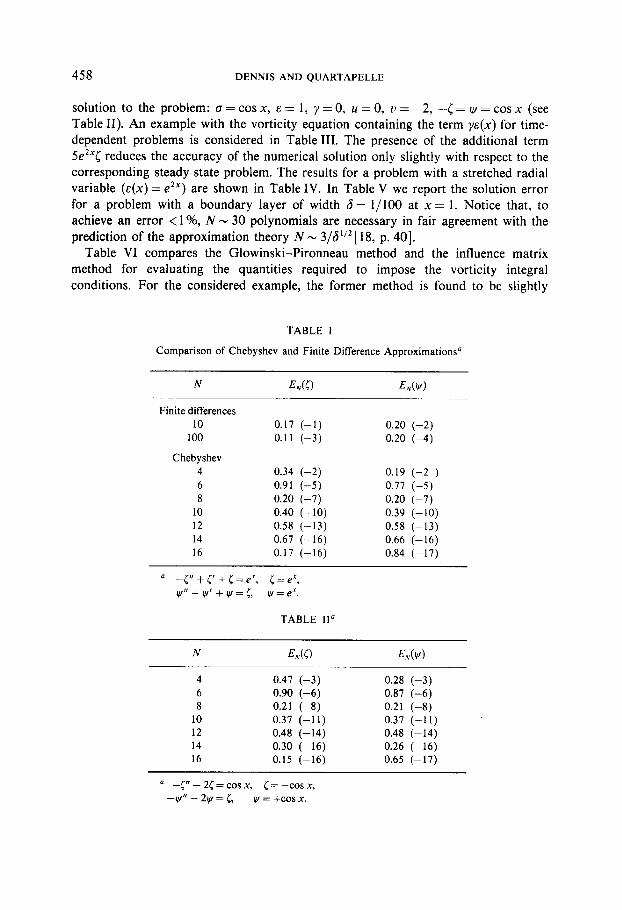
solution to the problem: u = cos x, E = 1, y = 0, u = 0, u = -2, -[ = ly = cos x (see Table II). An example with the vorticity equation containing the term YE(X) for time- dependent problems is considered in Table III. The presence of the additional term 5ezxc reduces the accuracy of the numerical solution only slightly with respect to the corresponding steady-state problem. The results for a problem with a stretched radial variable (E(X) = eZX) are shown in Table IV. In Table V we report the solution error for a problem with a boundary layer of width 6 = l/100 at x = 1. Notice that, to achieve an error < 1 %, N - 30 polynomials are necessary in fair agreement with the prediction of the approximation theory N - 3/~Yl’~ [ 18, p. 401.

Table VI compares the Glowinski-Pironneau method and the influence matrix method for evaluating the quantities required to impose the vorticity integral conditions. For the considered example, the former method is found to be slightly

TABLE I

Comparison of Chebyshev and Finite Difference Approximations”

N Ed0 E,,,(W)

Finite differences 10

100

Chebyshev 4 6 8

10 12 14 16

0.17 (-1) 0.11 (-3)

0.34 (-2) 0.19 (-2 ) 0.91 (-5) 0.77 (-5) 0.20 (-7) 0.20 (-7) 0.40 (-10) 0.39 (-10) 0.58 (-13) 0.58 (-13) 0.67 (-16) 0.66 (-16) 0.17 (-16) 0.84 (-17)

0.20 (-2) 0.20 (-4)

(I --C" t i' t 4 = ex, < = ex,

-w"ty'+w=& yl=e*.

TABLE II”

N EAL;) E,(v)

4 0.47 (-3) 0.28 (-3) 6 0.90 (-6) 0.87 (-6) 8 0.21 (-8) 0.21 (-8)

10 0.37 (-11) 0.37 (-11) 12 0.48 (-14) 0.48 (-14) 14 0.30 (-16) 0.26 (-16) 16 0.15 (-16) 0.65 (-17)

a -5” - 25 = cos x, [ = -cos x, -yl” - 2yl= [, qJ = +cos x.


TABLE III

Equations for Time-Dependent Problems’

N

4 0.71 (-2) 6 0.10 (-4) 8 0.20 (-7)

10 0.39 (-10) 12 0.57 (-13) 14 0.68 (-16) 16 0.30 (-16)

EdC) E,(v)

0.18 (-2) 0.73 (-5) 0.19 (-7) 0.39 (-10) 0.58 (-13) 0.65 (-16) 0.50 (-17)

“-~“+21;+5eZ”<=a(x), [=ex-‘, -I/ + 2yl= c, w=,X-‘.

TABLE IV

Equations for the Case of a Stretched Radial Variable’

N EN EN(v)

4 0.10 (+1) 0.23 (+O) 6 0.88 (-2) 0.42 (-2) 8 0.82 (-4) 0.94 (-4)

10 0.69 (-6) 0.15 (-5) 12 0.57 (-8) 0.20 (-7) 14 0.40 (-10) 0.20 (-9) 16 0.23 (-12) 0.15 (-11)

TABLE V

Resolution of a Boundary Layer”

N E,(C) E,(v)

32 0.14 (-1) 0.38 (-1) 40 0.62 (-3) 0.92 (-3) 48 0.15 (-4) 0.15 (-4) 56 0.23 (-6) 0.17 (-6) 64 0.20 (-8) 0.14 (-8)

a --r”+5’+r=(-.4*+A+1)eA’X-1’, -I#’ + u/’ + I// = [, A = 100; c(x) = eAtx-‘), v(x) = e.r’r-“/(-A* + A + 1).


TABLE VI

Comparison of Different Methods for Evaluating the Quantities

for the Vorticity Integral Conditions”

N E,&) E,(v)

Glowinski- Pironneau method

4 6 8

10 12 14 16

Influence matrix method

4 6 8

10

12 14 16

0.34 (-2) 0.19 (-2) 0.91 (-5) 0.77 (-5) 0.20 (-7) 0.20 (-7) 0.40 (-10) 0.39 (-10) 0.58 (-13) 0.58 (-13) 0.67 (-16) 0.66 (-16) 0.61 (-17) 0.53 (-17)

0.12 (-1) 0.94 (-3) 0.52 (-4) 0.95 (-5) 0.13 (-6) 0.22 (-7) 0.26 (-9) 0.42 (-10) 0.38 (-12) 0.63 (-13) 0.41 (-15) 0.71 (-16) 0.35 (-16) 0.40 (-17)

TABLE VII

Vorticity Equation with Nonconstant Coefficients”

Edi)

Oy= 1, u=ff=l, E(X) = t+,

f(x) = sin 3x, g(x) = sin 2x, h(x)‘= sin x, c(x) = exe’, y(x) = -e3’-‘/5.


TABLE VIII

Stream Function Containing Components Which Are Solutions of the Homogeneous Equation”

N E,v(i) E,(v)

4 0.29 (-1) 6 0.12 (-3) 8 0.32 (-6)

10 0.78 (-9) 12 0.18 (-11) 14 0.36 (-14) 16 0.27 (-16)

0.27 (-2) 0.25 (-4) 0.17 (-6) 0.86 (-9) 0.32 (-11) 0.96 (-14) 0.22 (-16)

a 4” t i’ t i = u(x), -W”tY’tyl=G

y(x) = exm’ f e”“*+” + eA2(xm”, A,,, = (1 f \/3)/2.

more accurate, which means that A and p are evaluated more accurately by the integral expressions (5.4) and (5.7) than by the local (pointwise) expressions (6.2) and (6.3). In Table VII we give the numerical results for a test problem in which the vorticity equation contains terms with nonconstant coefficients. It turns out that the presence of such additional terms reduces slightly the accuracy of only [ with respect to the case with f = g = h = 0 (cf. Table IV). Table VIII gives the error for a problem such that w contains also component solutions of the homogeneous equation DI,Y = 0 associated to Dty = C. By comparing with the results of Table VI, we see that the accuracy of both [ and v is affected. In Table IX we consider the same test problem of Table VI but modified by the specification of the vorticity at x = - 1. The comparison indicates that the global accuracy for problems with only one or two

TABLE IX

Vorticity Integral Condition at Only One Boundary Point”

N E,di) E,(v)

4 0.19 (-2) 6 0.74 (-5) 8 0.20 (-7)

10 0.39 (-10) 12 0.58 (-13) 14 0.65 (-16) 16 0.64 (-17)

0.17 (-2) 0.76 (-5) 0.20 (-7) 0.39 (-10) 0.58 (-13) 0.65 (-16) 0.68 (-17)

a -C”+C+[=exm’, [(-l)=e-‘, $(+l)= 1, -w”+w’tw=L y/(--l) = em*, w(+l) = 1.


TABLE X

Nonlinear Equations”

N E,&) E,(Y)

Number of iterations

6 0.97 (-5) 0.77 (-5) 5 8 0.21 (-7) 0.20 (-7) 6

10 0.40 (-10) 0.35 (-10) 8 12 0.59 (-13) 0.58 (-13) 10 14 0.67 (-17) 0.66 (-16) 11 16 0.17 (-16) 0.65 (-17) 12

vorticity integral conditions are almost identical. The last example is the nonlinear system

with u = u = 1 and exact solution t; = w = ex- ‘. The simple iterative scheme defined by v/O = 0, L(t#-‘)c = u, Dty’= <‘, i= 1, 2,..., is employed. The iteration is terminated when EN(ci) < E,,,(c) and EN($) < E,,,(W). The error and the number of iterations given in Table X show that the number of iterations to obtain a given accuracy is independent of the resolution N.

8. CONCLUSIONS

A direct algorithm for solving Chebyshev approximations to the vorticity-stream function equations has been presented. The method determines noniteratively the vorticity boundary values that make the no-slip conditions exactly satisfied. This is accomplished by solving four linear systems of two uncoupled second-order differential equations similar to the original c-w equations, plus an additional linear system of two algebraic equations with two unknowns. Some test calculations have demonstrated the accuracy and the effectiveness of the method. The algorithm can be employed in conjuction with the truncated series expansion method for calculating two-dimensional viscous flows with no-slip conditions prescribed on only two opposite sides of the computational domain. The present approach can also be generalized to solve the biharmonic equation in a rectangular two-dimensional domain as a system of two Poisson equations. By using a double expansion in Chebyshev polynomials and employing a direct spectral solver for the Poisson


equation with Dirichlet boundary conditions [21], one obtains a linear problem similar to Eq. (4.5) with 2(N + M + 2) unknowns, N and A4 being the number of Chebyshev polynomials for the expansions in the two spatial directions.

REFERENCES

1. M. D. VAN DYKE, Stanford University SUDAER No. 247, 1965. 2. S. A. ORSZAG AND G. S. PATTERSON, Phys. Rev. Lett. 28 (1972), 76. 3. B. FORNBERG, J. Comput. Phys. 25 (1977), 1. 4. C. M. TANG, J. Comput. Phys. 32 (1979), 80. 5. S. C. R. DENNIS AND J. D. A. WALKER, J. Fluid Mech. 48 (1971), 771. 6. F. NIEUWSTADT AND H. B. KELLER, Comput. and Fluids 1 (1973), 59. 7. S. A. ORSZAG AND M. ISRAELI, “Numerical Models of Ocean Circulation,” ISBN O-309-02225-8,

National Academy of Sciences, Washington, D. C., 1975, p. 284. 8. V. A. PATEL, Comput. and Fluids 4 (1976), 13; J. Comput. Phys. 28 (1978), 14. 9. S. C. R. DENNIS, S. N. SINGH, AND D. B. INGHAM, J. Fluid Mech. 101 (1982), 257.

10. S. A. ORSZAG AND L. C. KELLS, J. Fluid Mech. 96 (1980), 159. 11. P. MOIN AND J. KIM, J. Comput. Phys. 35 (1980), 381. 12. L. KLEISER AND U. SCHUMANN, Treatment of incompressibility and boundary conditions in 3-D

numerical spectral simulations of plane channel flows,” in “Proceedings of the Third GAMM Conference on Numerical Methods in Fluid Mechanics” (E. H. Hirschel, ed.), p. 165, Vieweg. Braunshweig, 1980.

13. L. KLEISER, “Numerische Simulationen zum laminarturbulenten Umschlagsprozess der ebenen PoiseuilleStr6mung,” dissertation, Karlsruhe, April 1982.

14. L. QUARTAPELLE, J. Comput. Phys. 40 (1981), 453. 15. L. QUARTAPELLE AND M. NAPOLITANO, Int. J. Numer. Methods Fluids, to appear 1983. 16. R. GLOWINSKI AND 0. PIRONNEAU, SIAM Rev. 21 (1979), 167. 17. L. Fox AND I. PARKER, “Chebyshev Polynomials in Numerical Analysis,” Oxford Univ. Press,

London/New York, 1968. 18. D. GOTTLIEB AND S. A. ORSZAG “Numerical Analysis of Spectral Methods: Theory and

Applications,” Sot. Ind. Appl. Math., Philadelphia, 1977. 19. D. B. HAIDVOGEL, Quasigeostrophic regional and general circulation modelling: An efficient

pseudospectral approximation technique, in “Computing Methods in Geophysical Mechanics” (R. P. Shaw, ed.), Vol. 25, Amer. Sot. Mech. Engrs., New York, 1977.

20. S. A. ORSZAG, J. Comput. Phys. 37 (1980), 70. 21. D. B. HAIDVOGEL AND T. ZANG, J. Comput. Phys. 30 (1979), 167.

Direct Solution of the Vorticity-stream Function Ordinary Differential Equations by a Chebyshev...

Documents

Transcript of Direct Solution of the Vorticity-stream Function Ordinary Differential Equations by a Chebyshev...