Direct Passive Navigation

IEEE TRANSACTIONS ON PATTERN ANALYSIS AND MACHINE INTELLIGENCE, VOL. PAMI-9, NO. 1, JANUARY 1987

[28] Y. R. Wang, "Characterization of binary patterns and their projec-tions," IEEE Trans. Comput., vol. C-24, Oct. 1985.

[29] R. Y. Wong and E. L. Hall, "Scene matching with invariant mo-ments," Comput. Graphics Image Processing, vol. 8, no. 1, Aug.1978.

[30] Z. Q. Wu and A. Rosenfeld, "Filtered projections as an aid in cornerdetection," Pattern Recognition, vol. 16, no. 1, 1983.

[31] K. Yamamoto and S. Mori, "Recognition of handprinted charactersby outermost point methods," in Proc. Fourth Conf. Pattern Rec-ognition, Kyoto, Japan, 1978, pp. 794-796.

Direct Passive NavigationSHAHRIAR NEGAHDARIPOUR AND BERTHOLD K. P. HORN

Abstract-In this correspondence, we show how to recover the mo-tion of an observer relative to a planar surface from image brightnessderivatives. We do not compute the optical flow as an intermediatestep, only the spatial and temporal brightness gradients (at a minimumof eight points). We first present two iterative schemes for solving ninenonlinear equations in terms of the motion and surface parameters thatare derived from a least-squares fomulation. An initial pass over therelevant image region is used to accumulate a number of moments ofthe image brightness derivatives. All of the quantities used in the it-eration are efficiently computed from these totals without the need torefer back to the image. We then show that either of two possible so-lutions can be obtained in closed form. We first solve a linear matrixequation for the elements of a 3 x 3 matrix. The eigenvalue decom-position of the symmetric part of the matrix is then used to computethe motion parameters and the plane orientation. A new compact no-tation allows us to show easily that there are at most two planar solu-tions.

Index Terms-Eigenvalue decomposition, least-squares, optical flow,planar surfaces, structure and motion.

I. INTRODUCTION

The problem of recovering rigid body motion and surface struc-ture from image sequences has been the topic of many researchpapers in the area of machine vision (the reader is referred to asurvey of previous literature [1]). Two types of approaches, dis-

Manuscript received March 11, 1985; revised November 13, 1985 andApril 30, 1986. Recommended for acceptance by W. B. Thompson. Thiscorrespondence describes research done at the Artificial Intelligence Lab-oratory of the Massachusetts Institute of Technology and the RoboticsGroup of the University of Hawaii. The M.I.T. artificial intelligence re-search was supported in part by the Advanced Research Projects Agencyof the Department of Defense under Office of Naval Research ContractN00014-75-C-0643 and in part by the System Development Foundation.The University of Hawaii Robotics Group was supported in part by theNational Science Foundation.

S. Negahdaripour is with the Artificial Intelligence Laboratory, Mas-sachusetts Institute of Technology, Cambridge, MA 02139.

B. K. P. Horn is with the Department of Electrical Engineering, Uni-versity of Hawaii, Honolulu, HI 96822, on leave from the Artificial Intel-ligence Laboratory, Massachusetts Institute of Technology, Cambridge,MA 02139.

IEEE Log Number 8609967.Note: A paper describing the iterative solution to this problem was sub-

mitted by the authors on March 11, 1985 and accepted for publication onNovember 13, 1985. A second paper describing the closed form solutionwas submitted on November 18, 1985. At the suggestion of the reviewersand the Editor these two papers have been consolidated into one paper,which was accepted for publication on April 30, 1986.

crete and continuous, have been pursued. In the discrete approach,information about the displacements of a finite number of discretepoints in the image is used to reconstruct the motion. To do thisone has to identify and match feature points in a sequence of im-ages. The minimum number of points required depends on thenumber of images. In the continuous approach, the optical flow,that is the apparent velocity of image brightness patterns, is used.

In much of the work on recovering surface structure and motion,it is assumed that either a correspondence between a sufficient num-ber of feature points in successive frames has been established orthat a reasonable estimate of the full optical flow field is available.

In general, identifying features involves determining gray-levelcorner points. For images of smooth objects, it is difficult to findgood features or corners. Further, the correspondence problem hasto be solved, that is, feature points from consecutive frames haveto be matched.

The computation of the local flow field exploits a constraintequation between the local intensity changes and the two compo-nents of the optical flow. This only gives the component of flow inthe direction of the intensity gradient. To compute the full flowfield, one needs additional constraints such as the heuristic as-sumption that the flow field is locally smooth [4], [5]. This, inmany cases, leads to an estimated optical flow field that is not thesame as the true motion field.

In this corrspondence, we determine the motion of an observerrelative to a planar surface directly from the image brightness de-rivatives witho4t the need to compute the optical flow as an inter-mediate step. We restrict ourselves to planar surfaces since onlythree parameters are needed to specify the surface structure. Wewill first derive the image brightness constraint equation for thecase of rigid body motion. A least squares formulation allows usto derive nine nonlinear equations, the so-called planar motion fieldequations, in terms of the motion and surface parameters. We pre-sent two iterative schemes for solving these equations. It is shownthat all of the quantities used in the iteration can be computed ef-ficiently from a number of moments of the image brightness deriv-atives that are accumulated through an initial pass of over the rel-evant image region. We therefore do not have to refer back to theimage. We also show that a closed-form solution to the same prob-lem can be obtained through a two-step procedure. We first solvea linear matrix equation for the elements of a 3 x 3 matrix equationusing brightness derivatives (at a minimum of eight points). Theeigenvalue decomposition of the symmetric part of this matrix al-lows us to compute the motion parameters and the plane orientationeasily.

II. PRELIMINARIESWe first recall some details about perspective projection, the

motion field, the brightness change constraint equation, rigid bodymotion, and planar surfaces. This we do using vector notation inorder to keep the resulting equations as compact as possible.

A. Perspective ProjectionLet the center of projection be at the origin of a Cartesian co-

ordinate system. Without loss of generality we assume that the ef-fective focal length is unity. The image is formed on the plane z= 1, parallel to the xy-plane, that is, the optical axis lies along thez-axis. Let R be a point in the scene. Its projection in the image isr, where

R.R * z

The z-component of r is clearly equal to one, that is r = 1.

B. Motion FieldThe motion field is the vector field induced in the image plane

by the relative motion of the observer with respect to the environ-

0162-8828/87/0100-0168$01.00 © 1987 IEEE

168


ment. The optical flow is the apparent motion of brightness pat-tems. Under favorable circumstances the optical flow is identicalto the motion field. The velocity of the image r of a point R isgiven by

dr d 1=- R.

For convenience, we introduce the notation r, and R, for the timederivatives of r and R, respectively. We then have

1 1rt = R 2R,- (Rt 2)R,R^ (R )'

which can also be written in the cornpact form

1rt= (R )2 (Z x (Rt x R)),

since a x (b x c) = (c a)b - (a b)c. The vector rt lies in theimage plane, and so (r, * ) = 0. Further, rt = 0, if RtlIR, asexpected.

Finally, noting that R = (R z)r, we get

1rt= R (Z' x (Rt x r)).

C. Rigid Body MotionIn the case of the observer moving relative to a rigid environ-

ment with translational velocity t and rotational velocity o, we findthat the motion of a point in the environment relative to the ob-server is given by

Rt= - x R - t.

Since R = (R * z)r, we can write this as

R= -(R *z)c x r - t.

Substituting for Rt in the formula derived above for rt, we obtain

r,= -(x (rx (rx At))).

It is important to remember that there is an inherent ambiguity here,since the same motion field results when distance and the transla-tional velocity are multiplied by an arbitrary constant. This can beseen easily from the above equation since the same image planevelocity is obtained if one multiplies both R and t by some con-stant.

D. Brightness Change EquationThe brightness of the image of a particular patch of a surface

depends on many factors. It may for example vary with the orien-tation of the patch. In many cases, however, it remains at leastaproximately constant as the surface moves in the environment. Ifwe assume that the image brightness of a patch remains constant,we have

dEdt-

or

aE dr aEar dt at

where aElar = (aElax, aElay, 0) T is the image brightness gra-dient. It is convenient to use the notation Er for this quantity andE, for the time derivative of the brightness. Then we can write thebrightness change equation in the simple form

Er * rt + Et = 0.Substituting for r, we get

E- Er * x (r x (rx w - R =

Now

Er *( x (r x t)) = (Er x z) (r x t) = ((Er x z) x r) *

and by similar reasoning

Er * (2 x (r x (r x 0))) = (((Er x z) x r) x r) * ,

so we have

Et-(((Erxz) xr) xr) * X + ((Er XZ) xr) t=O.R iTo make this constraint equation more compact, let us define c =Et, s = (Er X z) x r, and v = -s x r; then, finally,

c + v * c + R s t = 0.

This is the brightness change equation in the case of rigid bodymotion.

E. Planar SurfaceA particularly impoverished scene is one consisting of a single

planar surface. The equation for such a surface is

R * n = 1,where nIn is a unit normal to the plane, and I/InI is the perpen-dicular distance of the plane from the origin. Since R = (R * z)r,we can write this as

1r * n =

so the constraint equation becomes

c + v * X + (r * n)(s t) = 0.

This is the brightness change equation for a planar surface.Note again the inherent ambiguity in the constraint equation. It

is satisfied equally well by two planes with the same orientationbut at different distances provided that the translational velocitiesare in the same proportions.

III. RECOVERING MOTION AND STRUCTUREGiven image brightness E(x, y, t), and its spatial and time de-

rivatives, Er and Et, over some region I in the image plane, we areto recover the translational and rotational motions, t and c, as wellas the plane n. Using the constraint equation developed above, wecould do this using image information at just a small number ofpoints. At each point we get one constraint and we have nine un-knowns to recover-or rather, eight, since we can recover the dis-tance of the plane and the translational velocity only up to a scalefactor. We will first present the iterative method. The motion pa-rameters and the plane orientation are obtained from the solutionof nine nonlinear equations derived from a least-squares formnula-tion for minimizing the error in the brightness change constraintequation. We then present the closed-form solution to the sameproblem that involves a two-step procedure. First, we solve fornine intermediate parameters, the elements of a 3 x 3 matrix, usingbrightness derivatives at a minimum of eight points. We then solvefor the motion parameters and the plane orientation from the ei-genvalue decomposition of the symmetric part of this matrix.

A. Iterative Method: Least-Squares FormulationImage brightness values are distorted with sensor noise and

quantization error. These inaccuracies are further accentuated bymethods used for estimating the brightness gradient. Thus it is notadvisable to base a method on measurements at just a few points.Instead we propose to minimize the error in the brightness con-straint equation over the whole region I in the image plane. So wewish to minimize

J = i [c + v - c + (r * n)(s. t)]2 dx dy

169

IEEE TRANSACTIONS ON PATTERN ANALYSIS AND MACHINE INTELLIGENCE, VOL. PAMI-9, NO. 1. JANUARY 1987

by suitable choice of the translational and rotational motion vectorst and o, as well as the normal to the plane n.

For an extremum of J we must have

-=0 ,-=0, and -=0.ac at anThat is,

| [c + v co + (r n) (s t)]v dx dy = 0,

(r n) [c + v co + (r n) (s t)]s dx dy = 0,

(s t)[c + v co + (r n)(s t)]r dx dy = 0.

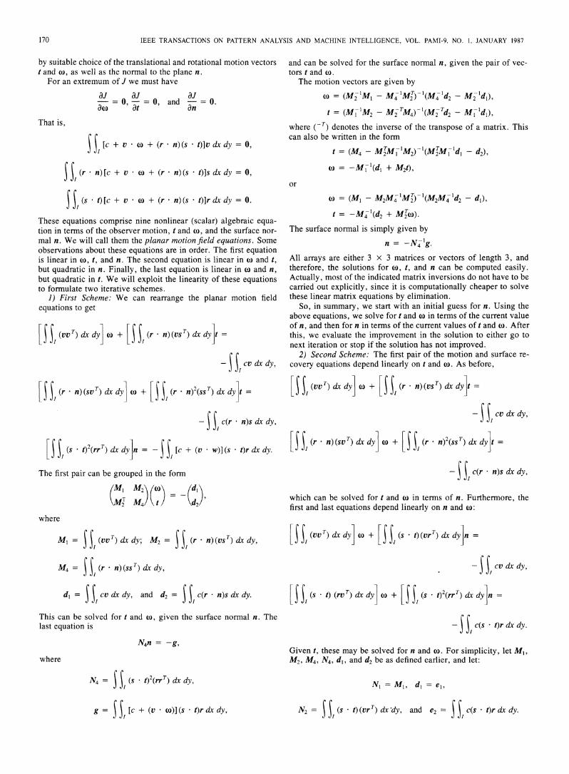
These equations comprise nine nonlinear (scalar) algebraic equa-tion in terms of the observer motion, t and c, and the surface nor-mal n. We will call them the planar motion field equations. Someobservations about these equations are in order. The first equationis linear in c, t, and n. The second equation is linear in o and t,but quadratic in n. Finally, the last equation is linear in o. and n,but quadratic in t. We will exploit the linearity of these equationsto formulate two iterative schemes.

1) First Scheme: We can rearrange the planar motion fieldequations to get

L|| (vvT)dxdyj c + (r n) (vs T) dx dyjt =

-|.| cv dx dy,

LH1(r * n)(svT) dx dy> o + Kl|(r * n)2(ssT) dx dyjt =

- | c(r - n)s dx dy,

and can be solved for the surface normal n, given the pair of vec-tors t and w.

The motion vectors are given by

X = (M2 AM - Ml4 M2T) '(M4 'd2 -M2 'dj),t =(Al-1M-2- M2TM4) -1(M -Td2 - MA 1dj),

where (-T) denotes the inverse of the transpose of a matrix. Thiscan also be written in the form

t - (M4 - M2jM1 1M2)-'(M2MI 1d1 - d2),

X = -M I(d1 + M2t),

or

X= (M1 - M2M4 1M2) -1(M2M4 1d2 - dl),

t = -Al4 '(d2 + M2T).The surface normal is simply given by

n = -N4 1g.All arrays are either 3 x 3 matrices or vectors of length 3, andtherefore, the solutions for w, t, and n can be computed easily.Actually, most of the indicated matrix inversions do not have to becarried out explicitly, since it is computationally cheaper to solvethese linear matrix equations by elimination.

So, in summary, we start with an initial guess for n. Using theabove equations, we solve for t and w in terms of the current valueof n, and then for n in terms of the current values of t and c. Afterthis, we evaluate the improvement in the solution to either go tonext iteration or stop if the solution has not improved.

2) Second Scheme: The first pair of the motion and surface re-covery equations depend linearly on t and w. As before,

i(VVT) dx dy1 c + L (r n) (vsT) dx dylt=

-.|| cv dx dy,

r)2 d|jn (r n)(svT) dx dy X + [ I. | (r E n)2(ssT) dx dyjt =IJ s )(r)d yn = - Is[c + (v w)] (s t)Ordx dy. I I

The first pair can be grouped in the form

( M20 (10\MTM4/ \ t/

(dI2

where

m1 = (vvT)dxdy; M2 = ||( n)(vsT)dxdy,

M4 = (r *n)(ssT) dx dy,

di= Sj cv dx dy, and d2 = ||c(r * n)s dx dy.

This can be solved for t and o, given the surface normal n. Thelast equation is

N4n = -g,

where

N4 = |(s *)2(rrT) dx dy,

c(r * n)s dx dy,

which can be solved for t and co in tenrms of n. Furthenmore, thefirst and last equations depend linearly on n and c:

(vv T) dx dyj + | (s It) (vrT)dx dyn =

-| & cv dx dy,

(s* t) (rv T) dx dyj X + (s * I)2(rrT) dx dyjn =

- ,V c(s * t)rdx dy.

Given t, these may be solved for n and o. For simplicity, let M1,M2, M4, N4, dl, and d2 be as defined earlier, and let:

N, = M1, d, = e ,

N2 = . (s * t)(vrT) dx-dy, and e2 = , c(s t)r dx dy.g = [c + (v w)](s * t)rdx dy,

170


Then

(MI M2\ (OP

MlT M4/\\ t /

and

(N1 N20 (coNT N41 nJ

The solution of the above equations is given by

X = (M2-'M1 - M4 M2T) '(M4 'd2 - M2 'd),

t = (MA1 M2 M2-TM4)- (MA2 Td2 M, 1dl),

and

c = (N -'N, - N-NT) -'(N -e2 N -le),

(N-'N2 N-TN4)- '(N-T2 N- le).

These may be rewritten in either of two asymmetrical forms shownearlier.

Again, most of the indicated matrix inversions do not have to becarried out explicitly, since we can solve the equations by elimi-nation.

In this scheme, we start with an initial guess for n. We solve fort and co in terms of the current value of n, and update t, then solvefor n and X in terms of the current value of t, and update n, and,finally, evaluate the improvement in the solution to either continuewith the next iteration or stop if the solution has not improved.

3) Division ofLabor: These methods would not be very attrac-tive, if we had to perform integrations over the whole image regionI during each iteration, in order to collect the matrices and vectorsappearing in the equations. Fortunately, this is not necessary. Onecan see this by writing the equations for the components of thematrices and vectors using the summation convention of tensor cal-culus (that is, there is an implicit summation over any index thatappears twice in an expression):

{Mlij=X ivjad dy.,

{M2}ij = |Visjrk dx dy1nk,

{} ij = |ssj rkrl dx dy]nknl,

{dl} -i cvi dx dy, {d2} = L csi rj dx dy1nj,

{Nl}ij= v|vvjdxdy,

{N2}ij= K1ViSkrjdXdY1tk,

{N41ij = jSkSlrirj dr dy]tktl,

-el}i= jcvidxdy, {e2}i= L||csIr,dxdyjt,

and

{g}i = L crisj dx dy tj + k|kri vj dYjtkwj

Ml = N, and d, = el do not depend on o, t, or n, and so needonly be computed once. Also, (cvi), (vivj), (csirj), (rkvisj), and

(rk r, si sj) depend only on r, Er, and E,, and so can be integratedover the image once. This appears to be a set of 3 + 9 + 9 + 27+ 81 = 129 numbers, but, because of symmetry in (vivj), and(rkrlsisi), only 81 numbers have to be stored. These accumulatedtotals represent all the image information needed to solve the mo-tion recovery problem.

In the first scheme, we only perform 279 multiplications per it-eration; The updating of the coefficients of the planar motion fieldequations involves 27 + 9 + 42 + 42 + 42 = 162 multiplicationsto compute M2, d2, M4, N4, and g (note that M4 and N4 are sym-metric). The updating of c, t, and n, in comparison, requires 117multiplications.

In the second scheme, 696 multiplications are carried out at eachiteration; we compute the matrices M2, M4 and the vector d2, re-quired for the first half of the iteration, in 27 + 42 + 9 = 78multiplications. The same number of multiplications is needed tocompute the matrices N2, N4 and the vector e2 required in the sec-ond half. Further, solving for X and t takes about 270 multiplica-tions, as does solving for w and n in the second half of each iter-ative step.

Through a selected example, we will show that the secondscheme has a much better convergence rate at the expense of morecomputation per iteration.

B. Uniqueness

It is important to establish whether more than one solution ispossible. In general, this is clearly so, since an image of uniformbrightness could correspond to an arbitrary uniform surface movingin an arbitrary way. So the brightness gradients, or lack of bright-ness gradients, can conspire to make the problem highly ambigu-ous. What we are interested in here is whether two different planarsurfaces can give rise to the same motion field given two differenttranslational and rotational motions of the imaging system.

In our terms then, the question becomes: given that the bright-ness change equation is satisfied for the motion t and w and theplanar surface n, is there another motion t' and c' and anotherplanar surface n' that satisfies the same equation at all points in theregion I and for all possible ways of marking the surface? Note thatwe have to consider a whole image region, since the problem isunderconstrained if we only have information along a line or at apoint in the image. We also have to include the condition that theconstraint should be satisfied for all possible surface markings toavoid the kind of ambiguity discussed above, where brightness gra-dients fortuitously line up with the motion field to create ambigu-ity.

1) Dual Solution: Suppose that two motions and two planar sur-faces satisfy the brightness change equation. Then, we have

C + v * X + (r * n) (s - t) = 0,

C + v o' + (r - n')(s * t') - 0.

Subtracting these equations, we get

v (c - wo') + (r * n)(s - t) - (r - n')(s * t') = 0.

Now v = -s x r, so

-(s X r) * (o - wo') + (r * n)(s t) - (r * n')(s t') = 0,

or

-r ((X- c') x s) + (r * n)(s * t) -(r * n')(s * t') = 0.

If we let o = (cWI, C02, Cv3)T then we can write

O 0i3 + W2co x s = s, where Q = 0)3° -cot,

W2 +WI 0°is a suitable (3 x 3) skew-symmetric matrix. The (i, j)th elementof Q equals WkEijk, where Eijk iS the permutation symbol. (It equals+1 when the ordered set i, j, k is obtained by an even permutation

171

di

el

e2


of the set 1, 2, and 3, it equals - 1 when the ordered set is obtainedby an odd permutation, and it is zero if two or more of the indexesare equal.)

Using this notation we can now write

-rT(Q -T s + rT(ntT) s - rT(n'ttT)s = 0,

or just

rT[_(j1- Q') + ntT - n't,T]s = 0.

This is to be true for all points r in the image region I and allpossible brightness gradients. So

(Q- Qf) + ntT - n't'T = 0,

where the zero on the right-hand side here represents a 3 x 3 ma-trix of zeros. Now QjT = _ , since Q is a skew-symmetric, sotaking the transpose of the equation we get

+(- Q) + tn T- t'n'T = 0.

Adding the two equations allows us to eliminate (Q - a'), andwe end up with

(ntT + tnT) = (nYtT + t'n T).

The trace (sum of the diagonal elements) of ntT is just (n t), sowe see immediately that (n t) = (n' * t'T). But the above matrixequation involving the dyadic products of n and t as well as of n'and t' is much more constraining.

Consider the following three possibilities:1) If In' = 0 or It' = 0, then their dyadic product is a 3 x 3

matrix of zeros. In this case the above equation is satisfied if andonly if Int = 0 or itl = 0.

2) If n'tlln, t'l|t and tntIt't = tnt Itt, then the two sums of dyadicproducts are equal and the above equation is satisfied.

3) If n'ttt, t'tln and ln't It't = tnt itl, then the two sums of dyadicproducts are also equal and the above equation is satisfied.

It turns out that there are no other ways to satisfy the equation.This can be shown using elementary properties of dyadic products(see [8]) or by inspection of the six components of the above equa-tion (because of symmetry there are only six independent compo-nents).

The first case above corresponds to purely rotational motion,because either the translational motion is zero, or the planar surfaceis infinitely far away, and the translation does not generate a per-ceptible component of the motion field. The solution is unique inthis case, because we find (Q- E') = 0, when we substitute backinto the matrix equation. (This is nothing new, since it has beenknown for some time that the solution is unique in the case of purelyrotational and purely translational motion [2].)

In the second case we find that ntT = nIt'T, since the vectors areparallel and the product of their size is constrained by the conditionn * t = n' * t', derived earlier. Thus once again (Q- Q') = 0.Nothing new is obtained here, since we already know that we canchange the lengths of the vectors n and t as long as the product oftheir lengths remains constant.

The third case is the most interesting. Here we have tnT =n't"T so that

Q Q') + (nt T _ tnT) = 0,

and thus- Q') x + (ntT - tnT)x = 0,

for an arbitrary vector x. That is,

x x (c - o') + x x (n x t) = 0,

for an arbitrary vector x, so that

Xl - (0' + fl x t = 0,

or o' = X + n x t. To summarize then, if we ignore scaling ofthe normal and the translational velocity, we obtain a dual solution,

TABLE ITHE TRUE MOTION AND SURFACE PARAMETERS, AND A SUMMARY OF THERESULTS OF A SIMULATION THAT CONVERGES TO THE TRUE SOLUTION

USING THE FIRST SCHEME

True Rotational Motion Parameters wl = .003 w2 = .001 U3 = -.01True Translational Motion Parameters ti = .0005 t2 = -.005 t3 = .0125True Parameters of the Surface n, = .2 n2 = .4 n3 = 1.0

Initial Guess for the Simulation

Iter. (Rotational Par's)No. WI W2 W3

10152025303540455055606570

.00531

.00429

.00353

.00318

.00305

.00302

.00300

.00300

.00300

.00300

.00300

.00300

.00300

.00260

.00178

.00137

.00117

.00107

.00103

.00101

.00101

.00100

.00100

.00100

.00100

.00100

n5 = 100. n2= 5- n3 = -1.

(Translational Par's)t1 t2 t3

(Surface Par's)ni n2 n3

-.01016 -.00069 -.00284 .01301 .35524 .1923-.01008 -.00006 -.00384 .01291 .27623 .2742-.01002-.01000-.01000-.01000-.01000-.01000-.01000-.01000-.01000-.01000-.01000

.00024

.00038

.00045

.00048

.00049

.00050

.00050

.00050

.00050

.00050

.00050

-.00454 .01270-.00485 .01257-.00495 .01252-.00499 .01250-.00500 .01250-.00500 .01250-.00500 .01250-.00500 .01250-.00500 .01250-.00500 .01250-.00500 .01250

.23725

.21718

.20755

.20323

.20137

.20058

.20024

.20010

.20004

.20002

.20000

.3448

.3814

.3945

.3984

.3996

.3999

.4000

.4000

.4000

.4000

.4000

1.1.1.1.1.1.1.1.1.1.1.1.1.

given by

n' t,t'=n and o' = +n Xt.

Hay was the first to show the existence of the dual solution [3],although the result has apparently been independently rediscoveredseveral times since then [6], [7], [9]. (The most recent papers [6],[7] came to our attention only after completion of our version ofthe proof.)

This dual solution is not different from the original one in thespecial case that the motion is perpendicular to the planar surface,that is, nitt. In this case the solution is unique. Further, if t =0, then n' * z = 0. This corresponds to a planar surface parallel tothe observer's line of sight, and may be considered to be a degen-erate case.

C. A Selected ExampleWe now present the results of a simulation. It is noteworthy to

mention that in all simulations performed, our algorithms haveconverged to a solution. However, the number of iterations forconvergence to a solution depends on the initial condition (as is thecase with all iterative schemes developed for solving nonlinearequations). In this example, we will demonstrate the sensitivity ofboth schemes to the initial condition. The image brightness func-tion was generated using a multiplicative sinusoidal pattern (onethat varies sinusoidally in both x and y directions), a 450 field ofview was assumed, and the image brightness gradients were com-puted analytically to avoid errors due to image brightness quanti-zation and finite difference approximations of the brightness gra-dient. In practice, the brightness at image points in two frameswould be discretized first, and the gradient computed using finitedifference methods.

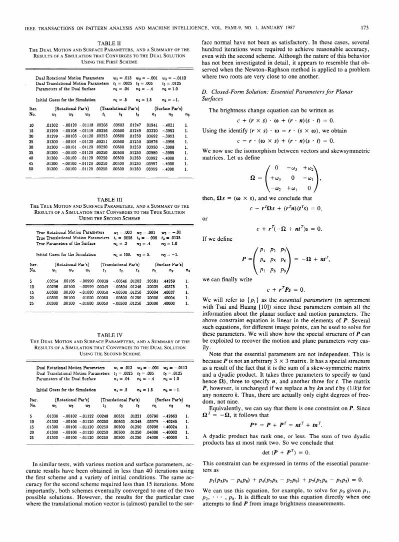
Table I shows the true motion and surface parameters, and theresults of a simulation that converged to the true solution using thefirst scheme described earlier. In Table II, the dual solution for thetrue motion and surface parameters, and the results of a simulationthat converged to the dual solution are tabulated. In both cases, thesolution after various number of iterations are given. The resultsshow that in the first case, the error in each parameter after lessthan 30 iterations is within 10 percent of the exact value. In thesecond case, this accuracy is achieved in less than 20 iterations.Similar results are presented in Tables III and IV for the secondscheme. Here, very good accuracy is achieved in less than 10 it-erations for the true solution and about 5 iterations for the dualsolution.

172


TABLE IITHE DUAL MOTION AND SURFACE PARAMETERS, AND A SUMMARY OF THERESULTS OF A SIMULATION THAT CONVERGES TO THE DUAL SOLUTION

USING THE FIRST SCHEME

Dual Rotational Motion Parameters wi1 = .013 W2 = -.001Dual Translational Motion Parameters ts = .0025 t2 = .005Parameters of the Dual Surface ni = .04 n2 = -.4


Iter. (Rotational Par's)No. ) W2 )W3

.01302

.01299

.01299

.01300

.01300

.01300

.01300

.01300

-.00120 -.01118-.00108 -.01119-.00103 -.01120-.00101 -.01120-.00101 -.01120-.00100 -.01120-.00100 -.01120-.00100 -.01120

W13 = -.0112t3 = .0125n3 = 1.0

nr = .5 n2 = 1.5 n3 = -1.

(Translational Par's)ts t2 t3

.002G6

.00256

.00253

.00251

.00250

.00250

.00250

.00250

.00503

.00500

.00500

.00500

.00500

.00500

.00500

.00500

.01247

.01249

.01250

.01250

.01250

.01250

.01250

.01250

(Surface Par's)n7 n2 n3

.01941

.03220

.03692

.03876

.03950

.03980

.03992

.03997

-.4021 1.-.3992 1.-.3993 1.-.3996 1.-.3998 1.-.3999 1.-.4000 1.-.4000 1.

50 .01300 -.00100 -.01120 .00250 .00500 .01250 .03999 -.4000 1.

TABLE IIITHE TRUE MOTION AND SURFACE PARAMETERS, AND A SUMMARY OF THERESULTS OF A SIMULATION THAT CONVERGES TO THE TRUE SOLUTION

USING THE SECOND SCHEME

True Rotational Motion Parameters wol = .003 W2 = .001 W3 = -.01True Translational Motion Parameters tl = .0005 t2 = -.005 t3 = .0125True Parameters of the Surface nv = .2 n2 = .4 n3 = 1.0


Iter. (Rotational Par's)No. usl so2 W3

nj = 100. n2 =5. n3 =-1.

(Translational Par's)ti t2. t3

.C0254 .00105 -.00990 .00039 -.00546 .01202

.GO296 .00100 -.00999 .00049 -.00504 .01246

.00300 .00100 -.01000 .00050 -.00500 .01250

.00300 .00100 -.01000 .00050 -.00500 .01250

.00300 .00100 -.01000 .00050 -.00500 .01250

(Surface Par's)ni n2 n3

.20581 .44259 1.

.20039 .40375 1.

.20004 .40037 1.

.20000 .40004 1.

.20000 .40000 1.

TABLE IVTHE DUAL MOTION AND SURFACE PARAMETERS, AND A SUMMARY OF THERESULTS OF A SIMULATION THAT CONVERGES TO THE DUAL SOLUTION

USING THE SECOND SCHEME

Dual Rotational Motion Parameters wos = .013 Wo2 = -.001 W3 = -.0112Dual Translational Motion Parameters t1 = .0025 t2 = .005 t3 = .0125Parameters of the Dual Surface n= .04 n2 = -.4 n3 = 1.0

Initial Guess for the Simulation n= .5 n2 = 1.5 n3 = -1.

Iter. (Rotational Par's) (Translational Par's) (Surface Par's)No. WIl 1u2 uW3 t5 t2 t3 n1 n2 n3

5 .01330 -.00102 -.01122 .00248 .00531 .01221 .03790 -.42663 1.10 .01303 -.00100 -.01120 .00250 .00503 .01248 .03979 -.40245 1.15 .01300 -.00100 -.01120 .00250 .00500 .01250 .03998 -.40024 1.20 .01300 -.00100 -.01120 .00250 .00500 .01250 .04000 -.40002 1.25 .01300 -.00100 -.01120 .00250 .00500 .01250 .04000 -.40000 1.

In similar tests, with various motion and surface parameters, ac-

curate results have been obtained in less than 40 iterations usingthe first scheme and a variety of initial conditions. The same ac-

curacy for the second scheme required less than 15 iterations. Moreimportantly, both schemes eventually converged to one of the twopossible solutions. However, the results for the particular case

where the translational motion vector is (almost) parallel to the sur-

face normal have not been as satisfactory. In these cases, severalhundred iterations were required to achieve reasonable accuracy,even with the second scheme. Although the nature of this behaviorhas not been investigated in detail, it appears to resemble that ob-served when the Newton-Raphson method is applied to a problemwhere two roots are very close to one another.

D. Closed-Form Solution: Essential Parameters for PlanarSurfaces

The brightness change equation can be written as

c + (r x s) o., + (r n)(s * t) = 0.

Using the identify (r x s) w0 = r (s x w), we obtain

c - r * (0 x s) + (r n)(s * t) = 0.

We now use the isomorphism between vectors and skewsymmetricmatrices. Let us define

/0 -L3 +W2\

Q= + (3 ° -WIl

<- 2 + (-1 °

then, Qs = (00 x s), and we conclude that

c - rTis + (rTn)(tTs) = 0,

or

c + rT(--fl + ntT)s = 0.

If we define

/ PI P2 P3\

P P4 P5 P6 =Q+ ntT

P7 P8 P9/we can finally write

c + rTPs = 0.

We will refer to {Pi } as the essential parameters (in agreementwith Tsai and Huang [10]) since these parameters contain all theinformation about the planar surface and motion parameters. Theabove constraint equation is linear in the elements of P. Severalsuch equations, for different image points, can be used to solve forthese parameters. We will show how the special structure of P canbe exploited to recover the motion and plane parameters very eas-ily.

Note that the essential parameters are not independent. This isbecause P is not an arbitrary 3 x 3 matrix. It has a special structureas a result of the fact that it is the sum of a skew-symmetric matrixand a dyadic product. It takes three parameters to specify 00 (andhence Ql), three to specify n, and another three for t. The matrixP, however, is unchanged if we replace n by kn and t by (I1k)t forany nonzero k. Thus, there are actually only eight degrees of free-dom, not nine.

Equivalently, we can say that there is one constraint on P. SinceQT = -Q2, it follows that

p* = p + pT = ntT + tn T.

A dyadic product has rank one, or less. The sum of two dyadicproducts has at most rank two. So we conclude that

det (P + pT) = 0.

This constraint can be expressed in terms of the essential parame-ters as

PI(PsP9 - P6P) + P4(P3P -P2P9) + P7(P2P6 - P3P5) = 0.

We can use this equation, for example, to solve for p9 given PI,P2, * * * , P8. It is difficult to use this equation directly when oneattempts to find P from image brightness measurements.

1015202530354045

510152025

173


There is a simple way around this problem, however. Note thatrTs = 0, because s = ((Er X z) x r). So rTIs = 0, and

c + rT(P + lI)s = 0,for arbitrary 1. If we let P' = P + II, we can write

c + rTP,s = 0,and conclude that we cannot recover P from image brightness mea-surements alone. To find P, we must impose the constraint det (P+ pT) = 0. To avoid dealing directly with the resulting nonlinearrelation between the essential parameters, we first find any P' thatsatisfies the above brightness change constraint equation for all im-age points being considered, and then determine 1 such that P =P' - II satisfies

det (P + pT) = 0.

Now,

det (P + pT) = det (P' + p,T - 211) = 0,so that 21 must be an eigenvalue of the real symmetric matrix

P -*= p' + p,TIt will become apparent, in the next section, that we ought to choosethe middle one of the three real eigenvalues of P'* for 21.

In summary, the overall plan is to find any matrix P' that satis-fies the image brightness constraint equation.

c + rTP,s = 0,at a suitable number of image points and consequently determineP'*. We can then solve for the middle eigenvalue of P'* (which is21) so as to construct the singular matrix P = P' - II, and fromthat we finally determine n and t as well as Q (and hence o) usingthe relationship

P= -Q + ntT.

1) Recovering Essential Parameters: We are looking for a ma-trix P' that satisfies the brightness change equation,

c + rTP,s = 0,

at a chosen number of image points. Now,rTP's = Trace {(srT)P'},

or

rTP's = Flat (srT) * Flat (P'),

where Flat (M) is the vector obtained from the matrix M by ad-joining its rows. So we can write the brightness change equationin the form

c + a p = 0,

where

Pi (pl, P2, * 9

a = (r1s1, rIs2, r1s3, r2s1, r2s2, r2s3, r3sI, r3s2, r3s3)T.

We first consider finding p' from the image brightness deriva-tives at the minimum number of points necessary. Later, we con-sider instead a least-squares procedure that takes into account in-formation in a whole image region.

From the derivatives of the brightness at the ith image point con-

sidered, we can construct the vector ai such that

aTp' = -c.

As discussed above, there are really only eight independent degreesof freedom. So we can arbitrarily fix one of the components of thevector p'. This means that we can solve for the other eight usingconstraint equations derived from eight image points.

Let p' = (pt, pt, ,p. , 0) T denote the solution obtained bysetting the last element equal to zero. If we define

a = (rlsl, rIS2, r1S3, r2s1, r2s2, r2S3, r3SI, r3S2),

then the above constraint equation reduces to

a T = -c.

Using eight independent points, we can solve the following linearmatrix equation:

Ap I = -c,where

The solution of the above equation is

p' = -A-1c.Image intensity values are corrupted with sensor noise and quan-

tization. These inaccuracies are further accentuated by methodsused for estimating the brightness gradient. Thus it is not advisableto base a method on measurements at just a few points. Instead wepropose to minimize the error in the brightness constraint equationover the whole region I in the image plane. So we choose the vectorp' that minimizes

| ~(dTpi + c)2 dxdy.

The solution, in this case, is given by

p= ( T dT dy) ca dx dy

In either case, we construct p' by adjoining a zero to the vectorp'. The result immediately gives us the matrix P'. We determinethe eigenvalues of P'* so that we can construct P* by subtractingthe identity matrix times twice the middle eigenvalue from P'*.We can also determine P by subtracting the identity matrix timesthe middle eigenvalue from P'. At this point, we are ready to re-cover t, o, and n.

Note that we do not have to repeat the eigenvalue-eigenvectoranalysis, since P* has the same eigenvectors as P'*, and its eigen-values are merely shifted so as to make the middle one equal tozero. This follows from the fact that if u and X are an eigenvector-eigenvalue pair of P'*, that is,

P'*u = Xu.then u and (X - 21) are an eigenvector-eigenvalue pair of P*,since

P*u = (P'* -21I) u = (X - 21)u.

2) Recovering Motion and Structure: We now show how tocompute the parameters of the translational motion and the planeorientation from the essential parameters. When we have done this,we will be able to also find the rotational parameters using

Q = ntT - P.

As we saw beforep* = p + pT = tnT + ntT,

since Q is skew-symmetric. Let us use the notation a = mnInti, andr = t, where

n tn =

In 1 and t= -

are the unit vectors in the directions of the surface normal and thetranslation vector, respectively. Then,

Trace (P*) = Trace (P) + Trace (pT) = 2n - t = 2or.

174


It turns out that nf and t can be easily recovered from the eigenvec-tors of the matrix P*. In the following lemma, we show that theeigenvectors of P* are combinations of the sought after vectors niand t.Lemma 1: Let P* = UAUT be the eigenvalue decomposition of

P (tnT + ntT). If n is not parallel to t, then,

A = Diag (r(T - 1), 0, a(r + 1)),

and,

U- t -n^ tn ti+ n 12(l1-rT)v -T 21+ )

Proof: Note that

P= u(t, T + nT).A~~~~~~~Now (t x n') is the eigenvector with eigenvalue zero since

P * (t x nf) = o(tnT + nt ) (t x n')= ut[fitfi] + an [tnit] = 0.

Since P* is real symmetric, it has three orthogonal eigenvectors.The other two eigenvectors must, therefore, be in the plane con-taining t and ni. Let u = at + fn^ and X denote an eigenvector-eigenvalue pair for some a and A (to be determined). Then,

a(t'nT + St)(at + ,3n) = X(at + ,Bn),

that becomes

o[a(t *i) + f3(nf ni)]t + a[al(t t) + 3(t ln)]nt = Xat + Xon3.Since (t = T, we can write

/rT - X af \/a 0

For this pair of homogeneous equations to have a nontrivial solu-tion for a and A, the determinant of the 2 x 2 coefficient matrixmust be zero, that is,

(r,T _ X)2 _ = 0,or

X U(r± 1).

Substituting for X into the earlier equations, we obtain

a = ±/.

Note that o(r - 1) < 0 and a(r + 1) > 0 because r < 1, as it isthe cosine of the angle between ni and t. So one eigenvalue is neg-ative and one is positive. (This is why we choose to make the mid-dle eigenvalue zero when constructing P* from P'*.) We find thateigenvectors corresponding to the eigenvalues XI = a(o - 1) andX3 = u(r + 1) are t - n' and t + ni, respectively. If we normalizethese, we obtain the unit vectors

t-nnt+_nul = , and U13 =

N2(1- T) s/2(1+ Tr)

Note that we can determine a = tlIti from

a = 2(X3 - X1)-

The equations for uI and U3 are linear in t and fi, and so can beeasily solved for these vectors:

n= (1 + T) 3- (l -)u

t^= +(l + T)U3 + V2(1- 7)UI.

The sign of the eigenvectors are arbitrary. If we change the sign oful, we obtain instead

2= ll+TU3 + V21(l - ')U11

t VI/(' + Tr)U3 - V2l(l - 'r)u1,where nt and t are interchanged. This is the dual solution.

The signs of the two eigenvectors can be chosen independently.This might suggest that there are a total of four different solutionsfor nf and t. We show next that two of these solutions can be dis-carded because they correspond to viewing the planar surface "frombehind." We assume that the visible part of the plane is the bound-ing surface of some solid object. We chose to define the orientationof the surface using the inward pointing normal n. The equation ofthe plane is R n = 1, or (r n) (R *z) = 1, since

R = (R )r.

Now, R * = Z is positive for points in front of the viewer, andso r * n must be positive for points on the visible portion of theplane. The equation r * n = 0 corresponds to a line in the image.Points on one side of this line, for which r * n > 0, can be imagesof points on the plane defined by the inward pointing normal n.Conversely, points on the other side of the line, where r * n < 0,cannot. They can be thought of as images of points on a parallelbut oppositely oriented plane corresponding to the vector -n. Weare analyzing brightness gradients for a particular image region. Ifr * n > 0 for points in this region, then n is a possible solution forthe surface normal. If r * n < 0 for points in this region, then -nis a possible solution. If r * n > 0 for some points and r * n < 0for others, then we are not dealing with the image of a single planarsurface.

Also, note that we can recover t and n up to a scale factor. Wecan let t to be a unit vector without loss of generality. Then, n canbe found as follows:

n = lnlJn = lnlltlnf = an,using the known value of a.

So far, we have assumed that n and t are not parallel. In thespecial case that tlIn, we have

P* = a(tiiT + t^iT) = 2annT

This dyadic product has rank one, that is, it only has one nonzeroeigenvalue. This is easy to show since any vector perpendicular tont is an eigenvector with zero eigenvalue. Also, fi is an eigenvectorwith eigenvalue 2a.

So if we find that P'* has two equal eigenvalues (that is P* hastwo zero eigenvalues), then we conclude that nf and t are paralleland equal to the eigenvector corresponding to the remaining eigen-value.We then solve for the rotation parameters by substituting the

solutions for n and t into the equation

Q = ntT- P.

Even though we gave a complete and compact proof of the dualsolution earlier, it is intriguing to confirm those results with ourclosed-form solution. We showed that the two solutions are relatedby

n'= lt, t' = (0' = 0) + n x t,

where we have arbitrarily set Itl = 1. The two solutions givenearlier for n and t already satisfy the duality relationship givenabove. The identity

(ntT - tnT) x = x x (n x t),

holds for any vector x. Using this in

WI X x = (c + n x t) x x = X x x + (n x t) x x,

we arrive at

w' x x = o x x - (ntT - tnT)x,

175


or

Q'x = (Q - ntT + tnT)x.

If this is to be true for all vectors x, we must have= Q- ntT + tnT

So, we finally obtain

-_' + n't'T = -_ + ntT -tnT + tnT,or,

-Q' + n't' = -Q + ntT= p.

We conclude that n', t', and c', as defined above, constitute asecond solution since they lead to the same set of essential param-eters.

IV. SUMMARYThe problem of recovering the motion of an observer relative to

a planar surface directly from the changing images (direct passivenavigation) was investigated and two solution procedures were pre-sented.We first formulated an unconstrained optimization problem.

Using conditions for optimality, it was reduced to solving a set ofnine simultaneous nonlinear equations that we termed the planarmotion field equations. Two iterative schemes for solving theseequations were given. It was shown that all information in the im-age concerning motion recovery can be captured by the momentsof the image brightness derivatives that constitute the coefficientsof the planar motion field equations. These moments are computedduring an initial pass over the relevant image regions so that thereis no need to refer back to the image after every iteration. Thisreduces the computation to accumulating 81 moments and perform-ing less than 300 multiplications per iteration in the first iterativescheme and approximately 700 multiplications in the second one.We also gave a compact proof that the problem can have at most

two planar solutions. Through a selected example with syntheticdata, it was shown that both schemes may converge to either of thetwo solutions, depending on the initial condition. In practice, oncea solution is obtained, the other can be computed using the equa-tions given for the dual solution.

In the tests carried out, both algorithms have converged to apossible solution, and accurate results have been obtained in lessthan 40 iterations using the first scheme, and in less than 15 itera-tions in the second one. As mentioned earlier, the results have not

been as satisfactory when the translational motion component isperpendicular to the planar surface. These cases required severalhundred iterations of either scheme for accurate solutions. It is con-ceivable that this special case that results in a unique planar solu-tion can be handled more appropriately by exploiting the fact thatthe translational motion is in the direction perpendicular to the sur-face.

Even though both schemes require approximately the same num-ber of computations for convergence to a solution (second schemeconverges faster but requires more computation), the second oneseems more appropriate for parallel implementation.We also presented a closed-fonn solution to the same problem.

We first employed the brightness change constraint equation thatwe developed for planar surfaces to compute 9 intermediate param-eters, the elements of a 3 x 3 matrix, from brightness derivativesat a minimum of eight image points. We referred to them as essen-tial parameters. The special structure of this matrix allows us tocompute the motion and plane parameters easily.

REFERENCES

[1] J. Barron, "A survey of approaches for determining optical flow, en-vironmental layout and egomotion," Univ. Toronto, Toronto, Ont.,Canada, Rep. RBCV-TR-84-5, Nov. 1984.

[2] A. R. Bruss and B. K. P. Horn, "Passive navigation," Comput. Vi-sion, Graphics, Image Processing, vol. 21, pp. 3-20, 1983.

[3] C. J. Hay, "Optical motion and space perception, an extention ofGibson's analysis," Psychol. Rev., vol. 73, pp. 550-565, 1966.

[4] E. C. Hildreth, 7he Measurement of Visual Motion. Cambridge,MA: M.I.T. Press, 1983.

[5] B. K. P. Horn and B. G. Schunk, "Determining optical flow," Ar-tificial Intell., vol. 17, pp. 185-203, 1981.

[6] H. C. Longuet-Higgins, "The visual ambiguity of a moving plane,"Proc. Roy. Soc. London, vol. B 223, pp. 165-175, 1984.

[7] S. J. Maybank, "The angular velocity associated with the optical flowfield due to a single moving rigid plane,'" in Proc. Sixth EuropeanConf. Artificial Intell., Sept. 1984, pp. 641-644.

[8] S. Negahdaripour and B. K. P. Horn, "Direct passive navigation,"M.I.T. A.I. Lab., Cambridge, MA, Al Memo 821, Feb. 1985.

[9] R. Y. Tsai, T. S. Huang, and W. L. Zhu, "Estimating three-dimen-sional motion parameters of a rigid planar patch, II: Singular valuedecomposition," IEEE Trans. Acoust., Speech, Signal Processing,vol. ASSP-30, Aug. 1982.

[10] R. Y. Tsai and T. S. Huang, "Uniqueness and estimation of three-dimensional motion parameters of rigid objects with curved sur-faces," IEEE Trans. Pattern Anal. Machine Intell., vol. PAMI-6,Jan. 1984.

176

Direct Passive Navigation

Documents

Transcript of Direct Passive Navigation