
Direct numerical prediction for the properties of complex ...
27
Direct numerical prediction for the properties of complex microstructure materials Andrei A. Gusev Institute of Polymers, Department of Materials, ETH-Zürich, Switzerland Outlook Unstructured mesh approach – Short fiber composites – Clay/Polymer nanocomposites for barrier applications – Voltage breakdown in random composites Regular grid approach – 3D X-ray micro-tomography – Aluminum infiltrated graphite matrix composites – Pglass/LDPE hybrid materials – Cellular materials
Transcript of Direct numerical prediction for the properties of complex ...

Direct numerical prediction for the propertiesof complex microstructure materials
Andrei A. Gusev
Institute of Polymers, Department of Materials, ETH-Zürich, Switzerland
Outlook
Unstructured mesh approach
– Short fiber composites
– Clay/Polymer nanocomposites for barrier applications
– Voltage breakdown in random composites
Regular grid approach
– 3D X-ray micro-tomography
– Aluminum infiltrated graphite matrix composites
– Pglass/LDPE hybrid materials
– Cellular materials
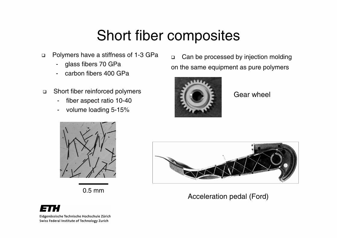
Short fiber compositesPolymers have a stiffness of 1-3 GPa
- glass fibers 70 GPa
- carbon fibers 400 GPa
Can be processed by injection molding
on the same equipment as pure polymers
Short fiber reinforced polymers
- fiber aspect ratio 10-40- volume loading 5-15%
Acceleration pedal (Ford)
Gear wheel
0.5 mm

Local fiber orientation statesArea with a high degree of orientation
Area with a low degree of orientation
Non-uniform fiber orientation states
⇒ non-uniform local material properties• stiffness
• thermal expansion• heat conductivity, etc.

Direct finite element predictionsPeriodic Monte Carlo configurations
– with non-overlapping spheres
– with non-overlapping fibers
Unstructured meshes (PALMYRA)– periodic morphology adaptive
– 107 tetrahedral elements
AAG, J. Mech. Phys. Solids, 1997, 45, 1449
AAG, Macromolecules, 2001, 34, 3081

ValidationShort glass-fiber-polypropylene granulate
– Hoechst, Grade 2U02 (8 vol. % fibers)– injection molded circular dumbbells
Image analysis– typical image frame (700x530 µm)
Measured fiber orientation distribution– transversely isotropic– statistics of 1.5·104 fibers
Measured phase properties– polypropylene matrix
E = 1.6 GPa, ν = 0.34, α = 1.1·10-4 K-1
– glass fibersE = 72 GPa, ν = 0.2, α = 4.9·10-6 K-1
– average fiber aspect ratio a = 37.3
0
100
200
300
0 30 60 90
angle θ
freq
uen
cy

ValidationMonte Carlo computer models
– 150 non-overlapping fibers
h PJ Hine, HR Lusti, AAGComp. Sci.Tecn. 2002, 62, 1927
h AAG, PJ Hine, IM WardComp. Sci.Tecn. 2000, 60, 535
Fiber orientation distribution– compared to the measured one
Effective properties
numerical measured
E11 [GPa] 5.14 ± 0.1 5.1 ± 0.25α11 [105·K-1] 3.1 ± 0.1 3.3 ± 1.5α33 [105·K-1] 11.7 ± 0.1 12.1 ± 0.2

Single fiber– unit vector p = (p1, p2, p3)
System with N fibers– 2nd order orientation tensor
– 4th order orientation tensor
Two step procedure
lkjiijkl ppppa =
1 φ
θ
p
2
3
Step 1: System with fully aligned fibers
– numerical prediction for Cijkl, αik, εik, etc.
Step 2: System with a given fiber orientation state
– orientation averaging– quick arithmetic calculation
jiij ppa =

Orientation averagingReference system with fully aligned fibers
– transversely isotropic
Effective elastic constants
A system with given aij and aijkl
Effective elastic constants
– Bi are related to the coefficients of Cref
AAG, Heggli, Lusti, Hine Adv. Eng. Mater. 2002– Direct & orientation averaging estimates– agree within 2-3%
⎟⎟⎟⎟⎟⎟⎟⎟
⎠
⎞
⎜⎜⎜⎜⎜⎜⎜⎜
⎝
⎛
=
66
66
44
222312
232212
121211
ref
00000
00000
00000
000
000
000
C
C
C
CCC
CCC
CCC
C
32
1
)()(
)(
542
31
jkiljlikklijijklklij
ikjliljkjkiljlikijkl
BBaaB
aaaaBaB
δδδδδδδδδδδδ
++++
++++=C

For transversely isotropic samples
As the trace of aij is 1, one needs only a11
Similarly, aijkl is solely determined by
Maximum entropy structures
⎟⎟⎟
⎠
⎞
⎜⎜⎜
⎝
⎛=
22
22
11
00
00
00
a
a
a
aij θ211 cos=a
θ41111 cos=a
The entropy of a system
pn is probability that the system is in state n
Maximum of S under a given a11
Comparison with image analysis data
nn
n ppS log∑−=
nnn θθθθ ∆+≤≤

Complex shape partsSteel molds (dies) are expensive
– on the order of $20k and more
Before any steel mold has been cut
– mold filling flow simulations
To optimize mold geometry & processing conditions• gate positions
• flow fronts
• local curing
• mold temperatures• cycle times
• etc.
Software vendors: Moldflow, Sigmasoft, etc.
– full 3D flow simulations instead of 2½ D
SigmaSoft GmbH, 2001

Computer-aided design of short fiber reinforced composite parts
MethodAAG, J. Mech. Phys. Solids, 1997, 45, 1449AAG, Macromolecules, 2001, 34, 3081
Short fibers:AAG, Hine, Ward, Comp. Sci.Tecn. 2000, 60, 535Hine, Lusti, AAG, Comp. Sci.Tecn. 2002, 62, 1445Lusti, Hine, AAG, Comp. Sci.Tecn. 2002, 62, 1927AAG, Lusti, Hine, Adv. Eng. Mater. 2002, 4, 927AAG, Heggli, Lusti, Hine, Adv. Eng. Mater. 2002, 4, 931Hine, Lusti, AAG, Comp. Sci.Tecn. 2004, 64, 1081
Spin-off company: MatSim GmbH, Zürich– Palmyra by MatSim, www.matsim.ch
Acknowledgements
– Professor U.W. Suter, ETH-Zürich
– Dr. P.J. Hine, IRC in Polymer Science & Technology, University of Leeds
– Dr. H.R. Lusti, ETH-Zürich– Professor I.M. Ward, University of Leeds
Performance of finished partAbaqus, Ansys, Nastran, etc.
Local material propertiesPalmyra + orientation averaging
Mold filling flow simulationsMoldFlow, SigmaSoft, etc.
Mold geometry,processing conditions

Voltage breakdown in random compositesDielectric parameters of pure polymers
– dielectric constants – voltage breakdown– determined by chemical composition– and processing route
Putting metal particles into polymers
– increasing dielectric constants– decreasing voltage breakdown
• local field magnifications
Periodic unstructured meshes– morphology-adaptive
Voltage breakdown mechanism– localized damage: pairs, triplets, etc– percolating path
E

Numerical procedureNumerical set up
– matrix: εM = 1& Ec = 1– inclusions: εI = 106
Apply a very small E– such that all local fields e are below Ec
Gradually increase E– when somewhere in the matrix e > Ec
– local voltage breakdown occurs– in the damaged sections, replace εM by εI
– go on
Computer model with 27 spheres– here, sphere volume fraction f = 0.3
Numerical predictions
– overall dielectric constant: εeff = 2.54– breakdown field: Eeff = 0.084– Adv. Eng. Mater. 5, 713 (2003)
E

Numerical predictionsNumerical estimates
– sphere volume fraction f = 0.1Composite voltage breakdown
– arrestingly, ensemble minimum valuesrepresentative already with only 8 spheres
Overall dielectric constants– remarkably, uniform RVE size is very small– ensemble vs. spatial averaging
Variable sphere volume loadings
Technological aspects
– relatively slow increase in εeff
– rapid decrease in Eef
0.0080.030.12Eeff
5.122.571.37εeff
0.50.30.1f

Aluminium / Graphite Composites
Squeeze casting process− graphite pre-form (porosity 14.5 vol-%)− infiltrated with aluminium melt (AlSi7Ba with 7 wt% Si & 0.25 wt% Ba )
3 phase composite: graphite (C), aluminium (Al), and pores
Al
C
Pore

3D X-ray tomography
Swiss Light Source (SLS)
Beamlines at SLS XTM (X-Ray Tomographic Microscopy)− at Materials Science beamline of SLS− beam energy of 10 keV
140 m
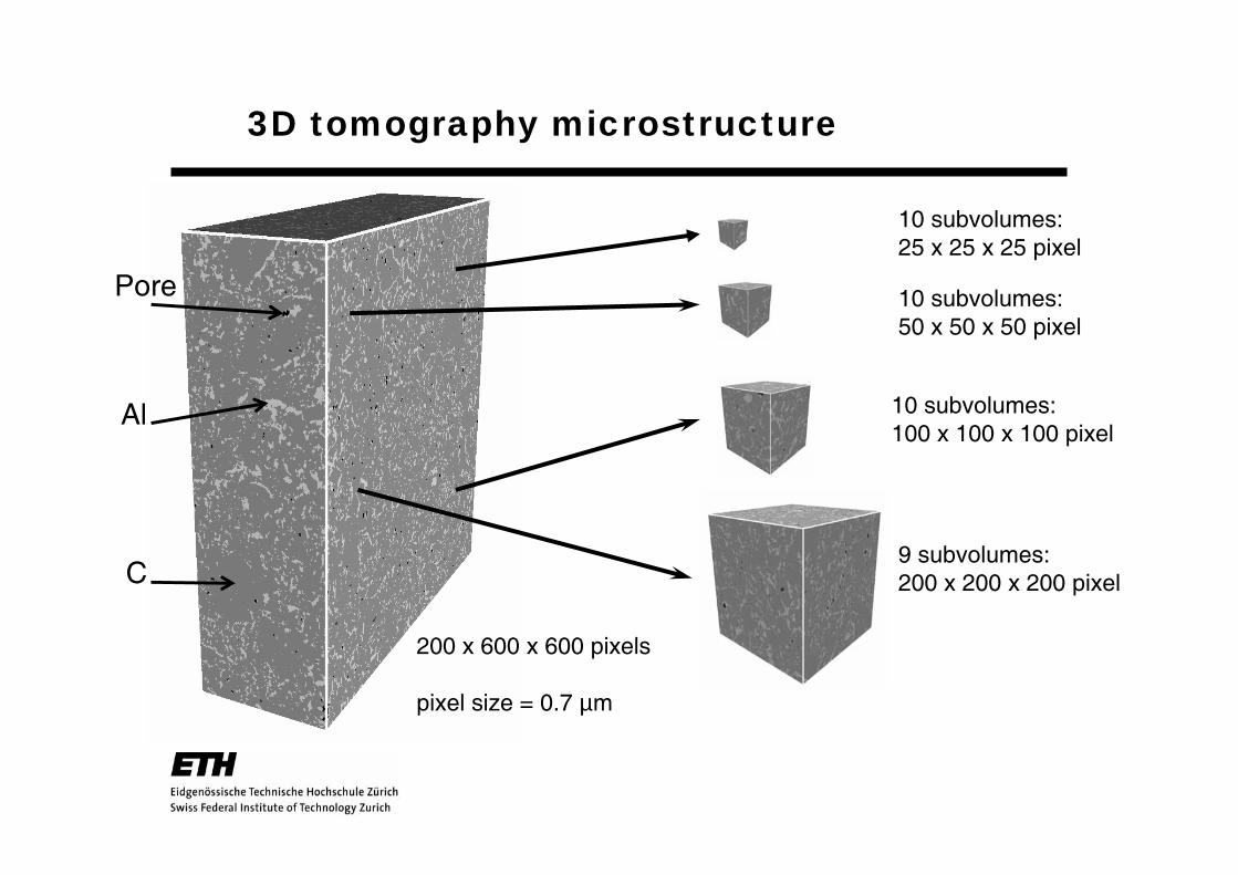
3D tomography microstructure
10 subvolumes:25 x 25 x 25 pixel
10 subvolumes:50 x 50 x 50 pixel
10 subvolumes:100 x 100 x 100 pixel
9 subvolumes:200 x 200 x 200 pixel
200 x 600 x 600 pixels
pixel size = 0.7 µm
Pore
Al
C

Effective conductivity
Technicalities:− serendipity family linear brick elements− iterative Krylov subspace solver− σeff from a linear response relation
Implementation− GRIDDER by MatSim GmbH
0gradφ)(σdiv =r
− for nodal potentials − with position dependent σ(r)
25 x 25 x 25 pixel model
FEM solution of Laplace’s equation
C
Al
Pore

Representative Volume Element Size
104 105 106 107 1080.01
0.1
1
10
N (number of pixels)
σ ef
f [10
6 /Ωm
] measured conductivity
upper Hashin-Shtrikman bound
lower Hashin-Shtrikman bound
Heggli, Etter, Uggowitzer, AAG, Adv. Eng. Mater. 2005 (accepted)

Pglass / Polymer hybrids
• Pglass: 0.5 SnF2 + 0.2 SnO + 0.3 P2O5− Tg ≈ 150 C− can be melt processed at ca. 200 C
• 50/50 (by volume) Pglass/LDPE hybrid− melt processed at about 200 C− J. Otaigbe of Univ. of Southern Mississippi− measured stiffness:
LDPE 0.2 GPaPglass 30 GPacomposite 1.2 GPa
Why is the composite stiffness so low ?Is the microstructure co-continuous ?
LDPEPglass
Adalja, Otaigbe, Thalacker, Polym. Eng. Sci. 2001, 41, 1055
DoM1

Slide 20
DoM1 Department of Materials, 2/1/2005

LDPE
Pglass
3D tomography microstructure
Numerical predictions for σeff assuming− either σ1 = 0 and σ2 = 1− or σ1 = 1 and σ2 = 0
Both phases percolateco-continuous microstructure
400 x 275 x 200 pixelspixel size ~ 5 µm

Property predictions (GRIDDER)
Predicted E is 7 times larger than the measured oneHypothesis: disintegration of Pglass phase
− under the influence of residual thermal stressesCritical sections:
− those with large von Mises stress & negative pressure
58
7.1
Effective
12150α [10-6/K]
300.2E [GPa]
PglassLDPE

Residual thermal stresses
( ) ( ) ( )[ ]213
232
2212
1 σσσσσστ −+−+−=
⎟⎟⎟
⎠
⎞
⎜⎜⎜
⎝
⎛=
332313
232212
131211
σσσσσσσσσ
σ
( )32131 σσσ ++=p
Local stress tensor
Pressure
Von Mises stress
Pglass, ∆T = -100 K

0.01 0.1 11E-3
0.01
0.1
1
E/E
s
Volume fraction
Stiffness of closed cell foams
Real foams:− with 1 < n < 2
Kirchhoff plate theory
− n = 1 reflects wall stretching− n = 3 reflects wall bending
Sparse form solver
− implemented in GRIDDER
27 cells
1024x1024x1024 grid
1E-3 0.01 0.1 10.0
0.5
1.0
1.5
C, n
Volume fraction
n
C
nss CEE )( ρρ=

Materials with cellular microstructure
Aluminum foam3D X-ray tomography
Closed cellcurved wall foam
Open cell foam
Understanding structure – property relationships− both 3D X-ray tomography and model microstructures− mechanical, thermal, electrical, and other properties

Conclusions & Perspectives
• Unstructured mesh approach (PALMYRA)– Linear tetrahedral elements– Remarkably efficient for object based representations– Currently: spheres, spheroids, platelets, and spherocylinders– Locking problems with fluids and rubbers
• Regular grid approach (GRIDDER)– Linear brick elements– Very large grids, 109 pixels and more– Appropriate for ordinary solids, rubbers and fluids– Property estimation companion for SCFT simulations
• For more on PALMYRA & GRIDDER technologies, visit www.matsim.ch


