Direct Multisearch for Multiobjective Optimization

DIRECT MULTISEARCH FOR MULTIOBJECTIVE OPTIMIZATION

A. L. CUSTODIO ∗, J. F. A. MADEIRA†, A. I. F. VAZ‡ , AND L. N. VICENTE§

Abstract. In practical applications of optimization it is common to have several conflictingobjective functions to optimize. Frequently, these functions are subject to noise or can be of black-box type, preventing the use of derivative-based techniques.

We propose a novel multiobjective derivative-free methodology, calling it direct multisearch(DMS), which does not aggregate any of the objective functions. Our framework is inspired bythe search/poll paradigm of direct-search methods of directional type and uses the concept of Paretodominance to maintain a list of nondominated points (from which the new iterates or poll centersare chosen). The aim of our method is to generate as many points in the Pareto front as possiblefrom the polling procedure itself, while keeping the whole framework general enough to accommodateother disseminating strategies, in particular when using the (here also) optional search step. DMSgeneralizes to multiobjective optimization (MOO) all direct-search methods of directional type.

We prove under the common assumptions used in direct search for single objective optimizationthat at least one limit point of the sequence of iterates generated by DMS lies in (a stationary formof) the Pareto front. However, extensive computational experience has shown that our methodologyhas an impressive capability of generating the whole Pareto front, even without using a search step.

Two by-products of this paper are (i) the development of a collection of test problems for MOOand (ii) the extension of performance and data profiles to MOO, allowing a comparison of severalsolvers on a large set of test problems, in terms of their efficiency and robustness to determine Paretofronts.

Key words. Multiobjective optimization, derivative-free optimization, direct-search methods,positive spanning sets, Pareto dominance, nonsmooth calculus, performance profiles, data profiles.

AMS subject classifications. 90C29, 90C30, 90C56.

1. Introduction. Many optimization problems involve the simultaneous opti-mization of different objectives or goals, often conflictual. In this paper, we areinterested in the development of derivative-free methods (see [9]) for Multiobjectiveoptimization (MOO). Such methods are appropriated when computing the derivativesof the functions involved is expensive, unreliable, or even impossible. Frequently, theterm black-box is used to describe objective and/or constraint functions for which,given a point, the value of the function is (hopefully) returned and no further in-formation is provided. The significant increase of computational power and softwaresophistication observed in the last decades opened the possibility of simulating largeand complex systems, leading to the optimization of expensive black-box functions.Such type of black-box functions also appear frequently in MOO problems (see, forinstance, [23]).

∗Department of Mathematics, FCT-UNL, Quinta da Torre, 2829-516 Caparica, Portugal([email protected]). Support for this author was provided by CMA/FCT/UNL under thegrant 2009 ISFL-1-297, and by FCT under the grant PTDC/MAT/098214/2008.

†IDMEC-IST, TU-Lisbon, Av. Rovisco Pais, 1040-001 Lisboa, Portugal and ISEL, Rua Conse-lheiro Emıdio Navarro, 1, 1959-007 Lisboa ([email protected]). Support for this author wasprovided by ISEL, IDMEC-IST, and FCT-POCI 2010.

‡Department of Production and Systems, University of Minho, Campus de Gualtar, 4710-057,Portugal ([email protected]). Support for this author was provided by Algoritmi Research Cen-ter and by FCT under the grant PTDC/MAT/098214/2008.

§CMUC, Department of Mathematics, University of Coimbra, 3001-454 Coimbra, Por-tugal ([email protected]). Support for this author was provided by FCT under the grantPTDC/MAT/098214/2008. Most of this work was developed while this author was visiting theCourant Institute of Mathematical Sciences of New York University under a FLAD scholarship.

1

In the classical literature of MOO, solution techniques are typically classified de-pending on the moment where the decision maker is able to establish preferences re-lating the different objectives (see [34]). Solution techniques with a prior articulationof preferences require an aggregation criterion before starting the optimization, com-bining the different objective functions into a single one. In the context of derivative-free optimization, this approach has been followed in [3, 32]. Different approachescan be considered when aggregating objectives, among which min-max formulations,weighted sums and nonlinear approaches (see, for instance, [42]), and goal program-ming [28]. In any case, the decision maker must associate weights or/and goals witheach objective function. Since the original MOO problem is then reduced to a singleobjective problem, a typical output will consist of a single nondominated point. If thepreferences of the decision maker change, the whole optimization procedure needs tobe reapplied.

Posteriori articulation of preferences solution techniques circumvent these diffi-culties, by trying to capture the whole Pareto front for the MOO problem. Weighted-sum approaches can also be part of these techniques, considering the weights as pa-rameters and varying them in order to capture the whole Pareto front. However, suchmethods might be time consuming and might not guarantee an even distribution ofpoints, specially when the Pareto front is nonconvex (see [13]). The normal boundaryintersection method [14] was proposed to address these difficulties, but it may pro-vide dominated points as part of the final output. The class of posteriori articulationof preferences techniques also includes heuristics such as genetic algorithms [41] andsimulated annealing [43].

The herein proposed algorithmic framework is a member of this latter class oftechniques, since it does not aggregate any of the objective functions. Instead, itdirectly extends, from single to multiobjective optimization, a popular class of di-rectional derivative-free methods, called direct search [9, Chapter 7]. Each iterationof these methods can be organized around a search step and a poll step. Given acurrent iterate (a poll center), the poll step in single objective optimization evaluatesthe objective function at some neighbor points defined by a positive spanning set anda step size parameter. We do the same for MOO but change the acceptance criterionof new iterates using Pareto dominance, which then requires the updating of a listof (feasible) nondominated points. At each iteration, polling is performed at a pointselected from this list and its success is dictated by changes in the list. Our frame-work encompasses a search step too, whose main purpose is to further disseminatethe search process of all the Pareto front.

We coined this new methodology direct multisearch (DMS) — as it reduces todirect search when there is only a single objective function. DMS extends to MOOall types of direct-search methods of directional type such as pattern search andgeneralized pattern search (GPS) [1, 30], generating set search (GSS) [30], and meshadaptive direct search (MADS) [2].

Our paper is divided as follows. Section 2 describes the proposed DMS algorithmicframework. An example illustrating how DMS works is described in Section 3. Theconvergence analysis can be found in Section 4 (and in an Appendix for the moretechnical details), where we prove, using Clarke’s nonsmooth calculus, that at leasta limit point of the sequence of iterates generated by DMS lies in (a stationary formof) the Pareto front.

Section 5 of this paper provides information about how our extensive numericalexperiments were performed, in particular we describe the set of test problems, the

2

solvers selected for comparison, the metrics used to assess the ability to computePareto fronts, and the use of performance and data profiles in MOO. In Section 6we report a summary of our computational findings, showing the effectiveness androbustness of DMS to compute a relatively accurate approximated Pareto front (evenwhen the initial list of nondominated points is initialized with a singleton and nosearch step is used). The paper ends with some final comments and discussion offuture work in Section 7.

In the remaining of the Introduction, we present concepts and terminology fromMOO used in our paper (see [36] for a more complete treatment). We pose a con-strained nonlinear MOO problem in the form:

min F (x) ≡ (f1(x), f2(x), . . . , fm(x))⊤

s.t. x ∈ Ω ⊆ Rn,

where we consider m (≥ 1) real-extended value objective functions or objective func-tion components fi : Rn → R ∪ +∞, i = 1, . . . ,m (forming the objective func-tion F (x)), and Ω represents the feasible region.

When several objective function components are present, given a point, it maybe impossible to find another one which simultaneously improves the value of all thefunctions at the given one. The concept of Pareto dominance is crucial for comparingany two points, and to describe it we will make use of the strict partial order inducedby the cone

Rm+ = z ∈ Rm : z ≥ 0,

defined by

F (x) ≺F F (y) ⇐⇒ F (y)− F (x) ∈ Rm+ \ 0.

Given two points x, y in Ω, we say that x ≺ y (x dominates y) when F (x) ≺F F (y).We will also say that a set of points in Ω is nondominated (or indifferent) when nopoint in the set is dominated by another one in the set.

As it is well known, the concept of minimization in single objective optimizationdoes not apply to MOO. In MOO problems it is common to have several conflictingobjective functions. Finding a point which corresponds to a minima for all the ob-jectives considered, meaning an ideal point, may be an unrealistic task. The conceptof Pareto dominance is used to characterize global and local optimality, by defining aPareto front or frontier as the set of points in Ω nondominated by any other one in Ω.

Definition 1.1. A point x∗ ∈ Ω is said to be a global Pareto minimizer of F inΩ if ∄y ∈ Ω such that y ≺ x∗. If there exists a neighborhood N (x∗) of x∗ such thatthe previous property holds in Ω ∩ N (x∗), then x∗ is called a local Pareto minimizerof F .

Rigorously speaking, the Pareto front is the set of global Pareto minimizers.However, the convergence results established for DMS are derived in terms of necessaryconditions for local Pareto minimization.

2. Direct multisearch for multiobjective optimization. In derivative-freeoptimization it is common to use an extreme barrier approach to deal with constraints.We adapt the extreme barrier function to multiobjective optimization (MOO) bysetting

FΩ(x) =

F (x) if x ∈ Ω,(+∞, . . . ,+∞)⊤ otherwise.

(2.1)

3

When a point is infeasible, the components of the objective function F are not evalu-ated, and the values of FΩ are set to +∞. This approach allows to deal with black-boxtype constraints, where only a yes/no type of answer is returned.

We present a general description for direct multisearch (DMS), which encom-passes algorithms using different globalization strategies, like those based on integerlattices and only requiring simple decrease of the objective function values for ac-cepting new iterates (see, for example, Generalized Pattern Search [1, 30] and MeshAdaptive Direct Search [2]), and also algorithms whose globalization strategy imposesa sufficient decrease condition for accepting new iterates (like Generating Set Searchmethods [30]).

Following the MOO terminology, described in the Introduction of the paper, theproposed algorithmic framework keeps a list of previously evaluated feasible nondo-minated points and corresponding step size parameters. This list plays an importantrole since it is what is returned to the user at the end of a run and since new iteratepoints (i.e., poll centers) are chosen from it. Also, as we will see later, success isdefined by a change in this list. Thus, we need to introduce the concept of iterate listin addition to the concept of iterate point (used in direct-search methods of directionaltype for single objective optimization).

As also happens for these methods in single objective optimization, each iterationis organized around a search step and a poll step, being the latter one responsible forthe convergence results. In DMS, the search step is also optional and used to possi-bly improve algorithmic performance. After having chosen one of the nondominatedpoints (stored in the current iterate list) as the iterate point (or poll center), each pollstep performs a local search around it.

In both the search and the poll steps, a temporary list of points is created first,which stores all the points in the current iterate list and all the points evaluatedduring the course of the step. This temporary list will then be filtered, removing allthe dominated points and keeping only the nondominated ones. Note that from (2.1),as we will later see in the description of the algorithm, the infeasible points evaluatedduring the course of the step are trivially removed.

The trial list is then extracted from this filtered list of feasible nondominatedpoints, and must necessarily include (for the purposes of the convergence theory) allthe nondominated points which belonged to the iterate list considered at the previousiteration. Different criteria can then be chosen to determine the trial list. A naturalpossibility is to define the trial list exactly as the filtered one. We will discuss thisissue in more detail after the presentation of the algorithmic framework. When thetrial list Ltrial is different from the current iterate list Lk, the new iterate list Lk+1

is set to Ltrial (successful search or poll step and iteration). Otherwise, Lk+1 = Lk

(unsuccessful poll step and iteration).

When using a sufficient decrease condition to achieve global convergence, onemakes use of a forcing function ρ : (0,+∞) → (0,+∞), i.e., a continuous and non-decreasing function satisfying ρ(t)/t → 0 when t ↓ 0 (see [30]). Typical examplesof forcing functions are ρ(t) = t1+a, for a > 0. To write the algorithm in generalterms, we will use ρ(·) to either represent the forcing function ρ(·) or the constant,zero function. Let D(L) be the set of points dominated by L and let D(L; a) ⊃ D(L)be the set of points whose distance in the ℓ∞ norm to D(L) is no larger than a > 0.For the purposes of the search step, we say that the point x is nondominated ifF (x) /∈ D(L; ρ(α)). When considering the poll step, the point x + αd is nondomi-nated if F (x+αd) /∈ D(L; ρ(α‖d‖)) (where d is a direction used in polling around x).

4

When ρ(·) is a forcing function requiring this improvement or decrease results in theimposition of a sufficient decrease condition.

As we will see later in the convergence analysis, the set of directions to be used forpolling is not required to positively span Rn (although for coherence with the smoothcase we will write it so in the algorithm below), and it is not necessarily drawn froma finite set of directions. In the following description of DMS, the elements of thelist are pairs of the form (x;α) but for simplicity we will continue to refer to thoseelements as points since in the majority of the cases our only interest is to appeal todominancy or nondominancy in the x part.

Algorithm 2.1 (Direct Multisearch for MOO).

Initialization

Choose x0 ∈ Ω with fi(x0) < +∞, ∀i ∈ 1, . . . ,m, α0 > 0, 0 < β1 ≤β2 < 1, and γ ≥ 1. Let D be a (possibly infinite) set of positive spanningsets. Initialize the list of nondominated points and corresponding step sizeparameters L0 = (x0;α0).

For k = 0, 1, 2, . . .

1. Selection of an iterate point: Order the list Lk in some way (somepossibilities are discussed later) and select the first item (x;α) ∈ Lk

as the current iterate and step size parameter (thus setting (xk;αk) =(x;α)).

2. Search step: Compute a finite set of points zss∈S (in a mesh ifρ(·) = 0, see Section A.1) and evaluate FΩ at each element. Set Ladd =(zs;αk), s ∈ S.Call Lfiltered = filter(Lk,Ladd) to eliminate dominated points fromLk ∪Ladd, using sufficient decrease to see if points in Ladd are nondom-inated relatively to Lk. Call Ltrial = select(Lfiltered) to determineLtrial ⊆ Lfiltered. If Ltrial 6= Lk declare the iteration (and the searchstep) successful, set Lk+1 = Ltrial, and skip the poll step.

3. Poll step: Choose a positive spanning set Dk from the set D. Eva-luate FΩ at the set of poll points Pk = xk + αkd : d ∈ Dk. SetLadd = (xk + αkd;αk), d ∈ Dk.Call Lfiltered = filter(Lk,Ladd) to eliminate dominated points fromLk ∪Ladd, using sufficient decrease to see if points in Ladd are nondom-inated relatively to Lk. Call Ltrial = select(Lfiltered) to determineLtrial ⊆ Lfiltered. If Ltrial 6= Lk declare the iteration (and the poll step)as successful and set Lk+1 = Ltrial. Otherwise, declare the iteration(and the poll step) unsuccessful and set Lk+1 = Lk.

4. Step size parameter update: If the iteration was successful thenmaintain or increase the corresponding step size parameters: αk,new

∈ [αk, γαk] and replace all the new points (xk + αkd;αk) in Lk+1 by(xk+αkd;αk,new), when success is coming from the poll step, or (zs;αk)in Lk+1 by (zs;αk,new), when success is coming from the search; replacealso (xk;αk), if in Lk+1, by (xk;αk,new).Otherwise decrease the step size parameter: αk,new ∈ [β1αk, β2αk] andreplace the poll pair (xk;αk) in Lk+1 by (xk;αk,new).

Next we address several issues left open during the discussion and presentationof the DMS framework.

List initialization. For simplicity, the algorithmic description presented initia-

5

lized the list with a single point, but different strategies, considering several feasiblepreviously evaluated points, can be used in this initialization, with the goal of im-proving the algorithmic performance. In Section 6.1, we suggest and numerically testthree possible ways of initializing the list. Note that a list initialization can also beregarded as a search step in iteration 0.

Ordering the iterate list. The number of elements stored in the list can varyfrom one to several, depending on the problem characteristics and also on the criteriaimplemented to determine the trial list. In a practical implementation, when theiterate list stores several points, it may be crucial to order it before selecting a pointfor polling, as a way of diversifying the search and explore different regions of Ω. Acrude ordering strategy could be, for instance, (i) to always add points to the end ofthe list and (ii) to move a point already selected as a poll center to the end of the list(doing it at the end of an iteration) for a better dissemination of the search of thePareto front. In Section 6.3 we will consider an ordering strategy defined by selectingthe poll centers using the values of a spread metric.

Search step and selection of the iterate point. The search step is optionaland, in the case of DMS (m > 1), it might act on the iterate list Lk rather than aroundan individual point. For consistency with single objective optimization (m = 1), weincluded the selection of the point iterate before the search step. If the search step isskipped or if it fails, this iterate point will then be the poll center. Another reasonfor this inclusion is to define a step size parameter for the search step.

Polling. As in single objective optimization, one either can have a complete pollstep, in which every poll point is evaluated, or an opportunistic poll step, in whichthe points in the poll set are sampled in a given order and sampling is stopped assoon as some form of improvement is found. In the algorithmic framework presentedabove, we have used complete polling, which can be a wise choice if the goal is tocompute the complete Pareto front. Opportunistic polling may be more suitable todeal with functions of considerably expensive evaluation. In this latter case, in orderto improve the algorithmic performance, the poll set should be appropriately orderedbefore polling [10, 12]. Since the convergence results will rely on the analysis of thealgorithmic behavior at unsuccessful iterations, which is identical independently ofthe polling strategy considered (opportunistic or complete), the results hold for bothvariants without any further modifications.

Filtering dominated points. Note that the filtering process of the dominatedpoints does not require comparisons among all the stored points since the currentiterate list Lk is already formed by nondominated points. Instead, only each addedpoint will be compared to the others, and, in particular, (i) if any of the points in thelist Lk ∪ Ladd dominates a point in Ladd, this added point will be discarded; (ii) ifan added point dominates any of the remaining points in the list Lk ∪ Ladd, all suchdominated points will be discarded. An algorithmic description of the procedure usedfor filtering the dominated points can be found in Figure 2.1.

Selecting the trial list. As we have pointed out before, a natural candidate forthe new iterate list is Ltrial = Lfiltered, in particular if our goal is to determine asmany points in the Pareto front as possible. However, other choices Ltrial ⊂ Lfiltered

can be considered. A more restrictive strategy, for instance, is to always consideran iterate list formed by a single point. In such a case, success is achieved if thenew iterate point dominates the current one. This type of algorithm fits in ourframework since it suffices to initialize the list as a singleton and to only consider inLtrial the point that dominates the one in Lk when it exists, or the point already

6

Algorithm 2.2: [L3]=filter(L1, L2)

Set L3 = L1 ∪ L2

for all x ∈ L2

do

for all y ∈ L3, y 6= x

do

if y ≺ xthen

L3 = L3\xif x ∈ L3

then

for all y ∈ L3, y 6= x

do

if x ≺ y

then

L3 = L3\yif y ∈ L2

then

L2 = L2\y

Fig. 2.1. Procedure for filtering the dominated points from L1 ∪ L2 (the set union should notallow element repetition), assuming that L1 is already formed by nondominated points.

Algorithm 2.3: [Ltrial]=select(Lfiltered)

Set Ltrial = Lfiltered

Algorithm 2.4: [Ltrial]=select(Lfiltered)

if Lk = xk * Lfiltered

then

Choose a x ∈ Lfiltered which dominated xk

Set Ltrial = xelse

Set Ltrial = Lk

Fig. 2.2. Two procedures for selecting the trial list Ltrial from the list of filtered nondominatedpoints Lfiltered. The list Lk represents the iterate list considered at the current iteration. Notethat in both algorithms all the nondominated points in Lk are included in Ltrial, as required for theconvergence theory.

in Lk, otherwise. An algorithmic description of these two procedures can be found inFigure 2.2.

3. A worked example. To illustrate how Algorithm 2.1 works, we will nowdescribe in detail its application to problem SP1 [25], defined by:

min F (x) ≡(

(x1 − 1)2 + (x1 − x2)2, (x1 − x2)

2 + (x2 − 3)2)⊤

s.t. − 1 ≤ x1 ≤ 5,

− 1 ≤ x2 ≤ 5.

As we will do later in Section 6.1 for the numerical experimentations, we willselect, here for the purposes of this example, the trial list from the filtered one as in

7

Algorithm 2.3 (setting Ltrial = Lfiltered). We will order the list by always addingpoints to the end of it and by moving a point already selected as a poll center to theend of the list (at the end of an iteration). No search step will be performed.

Initialization. Let us set the initial point x0 = (1.5, 1.5), corresponding to (f1(x0),f2(x0)) = (0.25, 2.25), and initialize the step size parameter as α0 = 1. The stepsize will be maintained at successful iterations and halved at unsuccessful ones, whichcorresponds to setting γ = 1 and β1 = β2 = 1

2 . Set D = D = [I2 −I2], where I2 standsfor the identity matrix of dimension 2. Initialize the iterate list of nondominated pointsas L0 = (x0; 1).

Iteration 0. The algorithm starts by selecting a point from L0, in this case the onlyavailable, (x0;α0). Since no search step is performed, the feasible points in the pollset P0 = (1.5, 1.5) + (1, 0), (1.5, 1.5) + (0, 1), (1.5, 1.5) + (−1, 0), (1.5, 1.5) + (0,−1)are evaluated (the filled diamonds plotted in Iteration 0 of Figure 3.1 represent thecorresponding function values). In this case, all the poll points were feasible, thus

Ladd = ((2.5, 1.5); 1), ((1.5, 2.5); 1), ((0.5, 1.5); 1), ((1.5, 0.5); 1).

The nondominated points are filtered from L0 ∪ Ladd, resulting in Lfiltered =((1.5, 1.5); 1), ((1.5, 2.5); 1). Only one of the evaluated poll points remained un-filtered (the circle in Iteration 0 of Figure 3.1 represents its corresponding functionvalue). According to Algorithm 2.3, Ltrial will coincide with Lfiltered. Since therewere changes in L0, the iteration is declared successful, and L1 = Ltrial = Lfiltered,being the step size maintained. The function values corresponding to the points in L1

are represented by squares in Iteration 0 of Figure 3.1. Note that we move the pollpoint to the end of the list, yielding the new order L1 = ((1.5, 2.5); 1), ((1.5, 1.5); 1).

Iteration 1. At the beginning of the new iteration, the algorithm selects a point fromthe two stored in L1. Suppose the point (x1;α1) = ((1.5, 2.5); 1) was selected. In thiscase, the poll set P1 = (2.5, 2.5), (1.5, 3.5), (0.5, 2.5), (1.5, 1.5) is evaluated (again,the corresponding function values are represented by filled diamonds in Iteration 1 ofFigure 3.1). Note that, by coincidence, two of the poll points share the same functionvalues. The list

Ladd = ((2.5, 2.5); 1), ((1.5, 3.5); 1), ((0.5, 2.5); 1), ((1.5, 1.5); 1)

is formed and L1 ∪ Ladd is filtered. Again, only one of the poll points was nondo-minated (the corresponding function value is represented by a circle in Iteration 1 ofFigure 3.1). Thus, the iteration was successful, the step size was maintained, and thenew list is

L2 = Ltrial = Lfiltered = ((1.5, 2.5); 1), ((1.5, 1.5); 1), ((2.5, 2.5); 1)

(the corresponding function values are represented by the squares in Iteration 1 ofFigure 3.1). Again, we move the poll point (in this case, ((1.5, 2.5); 1)) to the end ofthe list.

Iteration 2. The next iteration begins by selecting (x2;α2) = ((1.5, 1.5); 1) from thelist L2 (a previous poll center). After evaluating the corresponding poll points (the

8

0 0.5 1 1.5 2 2.5 3 3.51

2

3

4

5

6

7

8

Iteration0

f1

f2

0 0.5 1 1.5 2 2.5 3 3.5 4 4.50

1

2

3

4

5

6

7

8

Iteration1

f1

f2

0 0.5 1 1.5 2 2.5 3 3.5 4 4.50

1

2

3

4

5

6

7

8

Iteration2

f1

f2

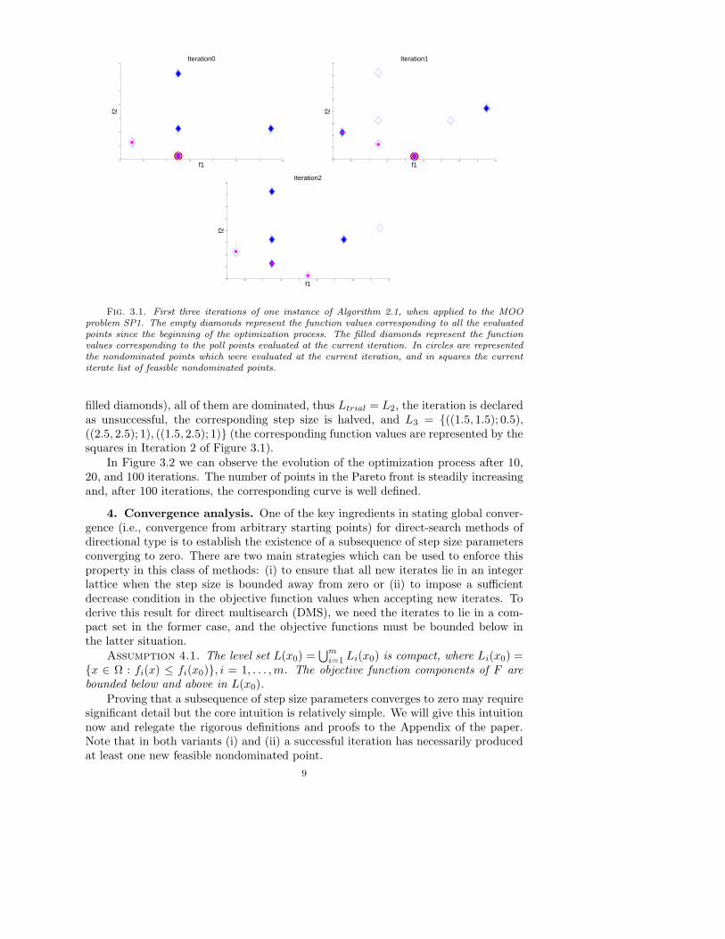
Fig. 3.1. First three iterations of one instance of Algorithm 2.1, when applied to the MOOproblem SP1. The empty diamonds represent the function values corresponding to all the evaluatedpoints since the beginning of the optimization process. The filled diamonds represent the functionvalues corresponding to the poll points evaluated at the current iteration. In circles are representedthe nondominated points which were evaluated at the current iteration, and in squares the currentiterate list of feasible nondominated points.

filled diamonds), all of them are dominated, thus Ltrial = L2, the iteration is declaredas unsuccessful, the corresponding step size is halved, and L3 = ((1.5, 1.5); 0.5),((2.5, 2.5); 1), ((1.5, 2.5); 1) (the corresponding function values are represented by thesquares in Iteration 2 of Figure 3.1).

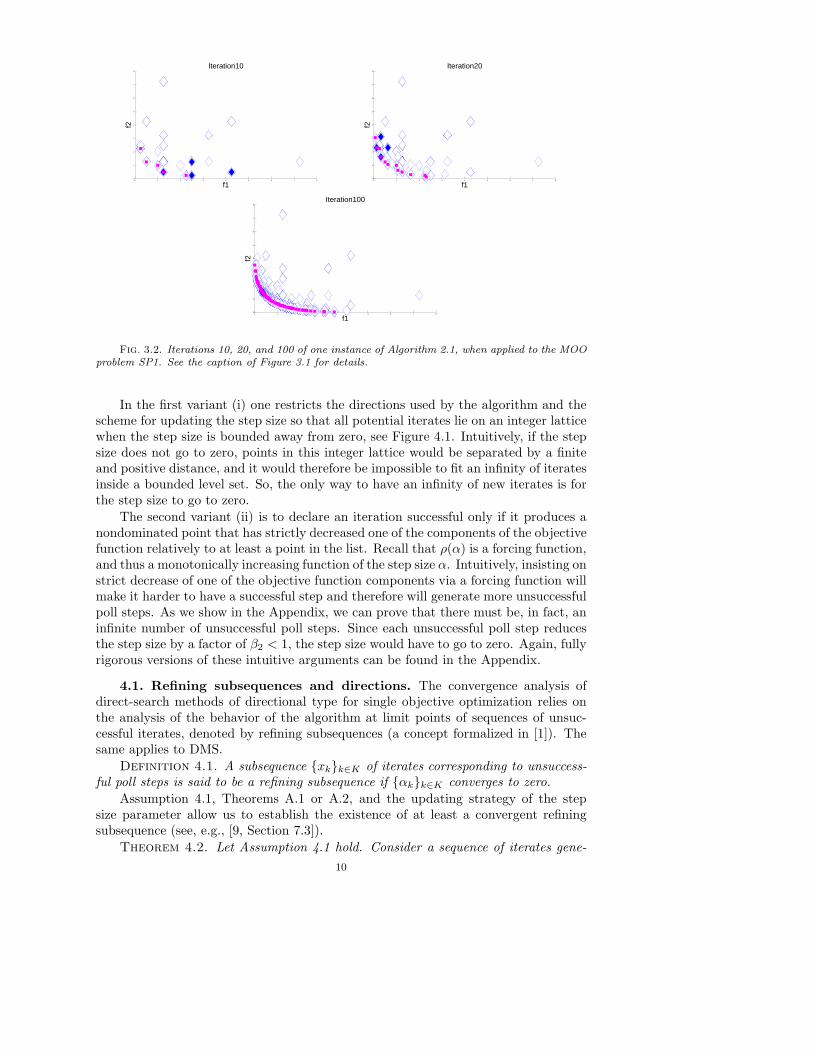
In Figure 3.2 we can observe the evolution of the optimization process after 10,20, and 100 iterations. The number of points in the Pareto front is steadily increasingand, after 100 iterations, the corresponding curve is well defined.

4. Convergence analysis. One of the key ingredients in stating global conver-gence (i.e., convergence from arbitrary starting points) for direct-search methods ofdirectional type is to establish the existence of a subsequence of step size parametersconverging to zero. There are two main strategies which can be used to enforce thisproperty in this class of methods: (i) to ensure that all new iterates lie in an integerlattice when the step size is bounded away from zero or (ii) to impose a sufficientdecrease condition in the objective function values when accepting new iterates. Toderive this result for direct multisearch (DMS), we need the iterates to lie in a com-pact set in the former case, and the objective functions must be bounded below inthe latter situation.

Assumption 4.1. The level set L(x0) =⋃m

i=1 Li(x0) is compact, where Li(x0) =x ∈ Ω : fi(x) ≤ fi(x0), i = 1, . . . ,m. The objective function components of F arebounded below and above in L(x0).

Proving that a subsequence of step size parameters converges to zero may requiresignificant detail but the core intuition is relatively simple. We will give this intuitionnow and relegate the rigorous definitions and proofs to the Appendix of the paper.Note that in both variants (i) and (ii) a successful iteration has necessarily producedat least one new feasible nondominated point.

9

0 1 2 3 4 5 6 7 80

1

2

3

4

5

6

7

8

Iteration10

f1

f2

0 1 2 3 4 5 6 7 80

1

2

3

4

5

6

7

8

Iteration20

f1

f2

0 1 2 3 4 5 6 7 80

1

2

3

4

5

6

7

8

Iteration100

f1

f2

Fig. 3.2. Iterations 10, 20, and 100 of one instance of Algorithm 2.1, when applied to the MOOproblem SP1. See the caption of Figure 3.1 for details.

In the first variant (i) one restricts the directions used by the algorithm and thescheme for updating the step size so that all potential iterates lie on an integer latticewhen the step size is bounded away from zero, see Figure 4.1. Intuitively, if the stepsize does not go to zero, points in this integer lattice would be separated by a finiteand positive distance, and it would therefore be impossible to fit an infinity of iteratesinside a bounded level set. So, the only way to have an infinity of new iterates is forthe step size to go to zero.

The second variant (ii) is to declare an iteration successful only if it produces anondominated point that has strictly decreased one of the components of the objectivefunction relatively to at least a point in the list. Recall that ρ(α) is a forcing function,and thus a monotonically increasing function of the step size α. Intuitively, insisting onstrict decrease of one of the objective function components via a forcing function willmake it harder to have a successful step and therefore will generate more unsuccessfulpoll steps. As we show in the Appendix, we can prove that there must be, in fact, aninfinite number of unsuccessful poll steps. Since each unsuccessful poll step reducesthe step size by a factor of β2 < 1, the step size would have to go to zero. Again, fullyrigorous versions of these intuitive arguments can be found in the Appendix.

4.1. Refining subsequences and directions. The convergence analysis ofdirect-search methods of directional type for single objective optimization relies onthe analysis of the behavior of the algorithm at limit points of sequences of unsuc-cessful iterates, denoted by refining subsequences (a concept formalized in [1]). Thesame applies to DMS.

Definition 4.1. A subsequence xkk∈K of iterates corresponding to unsuccess-ful poll steps is said to be a refining subsequence if αkk∈K converges to zero.

Assumption 4.1, Theorems A.1 or A.2, and the updating strategy of the stepsize parameter allow us to establish the existence of at least a convergent refiningsubsequence (see, e.g., [9, Section 7.3]).

Theorem 4.2. Let Assumption 4.1 hold. Consider a sequence of iterates gene-

10

x0

Fig. 4.1. An example of an integer lattice where all potential iterates must lie when the stepsize is bounded away from zero. The example corresponds to coordinate or compass search whereDk = [In − In] (In is the identity matrix of order n). The figure depicts a finite portion of that

integer lattice, which is given by x0 +α02r−

z : z ∈ Zn, where r− is some negative integer (see [9,Line 5 of Page 130]).

rated by Algorithm 2.1 under the scenarios of either Subsection A.1 (integer lattices)or Subsection A.2 (sufficient decrease). Then there is at least one convergent refiningsubsequence xkk∈K .

The first stationarity result in our paper will establish appropriate nonnegativityof generalized directional derivatives (see Definition 4.6) computed along certain limitdirections, designated as refining directions (a notion formalized in [2]).

Definition 4.3. Let x∗ be the limit point of a convergent refining subsequence.If the limit limk∈K′ dk/‖dk‖ exists, where K ′ ⊆ K and dk ∈ Dk, and if xk+αkdk ∈ Ω,for sufficiently large k ∈ K ′, then this limit is said to be a refining direction for x∗.

Note that refining directions exist trivially in the unconstrained case Ω = Rn.

4.2. Tangent cones and generalized derivatives. The main theoretical re-sult of this paper states that a limit point of the sequence of iterates generated bya DMS method is Pareto-Clarke stationary. In this subsection we introduce this de-finition of stationarity as well as other concepts related to nonsmooth calculus [7],required for the presentation and analysis of the DMS framework.

In single objective constrained optimization, a critical point has the property thatif one moves slightly away from it in any ‘feasible direction’, the objective functiondoes not improve. For multiobjective constrained optimization, the notion of criticalpoint changes somewhat. Essentially, a critical point will be a point on the local Paretofront (see Definition 1.1). As a result, it will have the property that moving slightlyaway from this point in any ‘feasible direction’ will not yield a better, dominatingpoint. This, in turn, means that as one moves away in a ‘feasible direction’, at leastone of the multiple objectives gets worse. We can formalize these intuitive ideas usingthe concept of Clarke tangent vector for the notion of ‘feasible direction’ and theconcept of Pareto-Clarke critical point for the notion of a ‘critical point on the Paretofront’. The definitions of these quantities are as follows.

We start by defining the Clarke tangent cone, which we will use to state Pareto-Clarke first-order stationarity. The Clarke tangent cone is a generalization of the

11

commonly used tangent cone in Nonlinear Programming (NLP) (see, e.g., [38, Defi-nition 12.2 and Figure 12.8]). Such generalization is convenient for our analysis, butshould not confuse a reader used to the basic definition of tangent cones in NLP. Thedefinition and notation are taken from [2].

Definition 4.4. A vector d ∈ Rn is said to be a Clarke tangent vector to the setΩ ⊆ Rn at the point x in the closure of Ω if for every sequence yk of elements of Ωthat converges to x and for every sequence of positive real numbers tk converging tozero, there exists a sequence of vectors wk converging to d such that yk+ tkwk ∈ Ω.

The set TClΩ (x) of all Clarke tangent vectors to Ω at x is called the Clarke tangent

cone to Ω at x.We will also need the definition of hypertangent cone since it is strongly related

to the type of iterates generated by a direct-search method of directional type. Thehypertangent cone is the interior of the Clarke tangent cone (when such interior isnonempty). Again we will follow the notation in [2].

Definition 4.5. A vector d ∈ Rn is said to be a hypertangent vector to the setΩ ⊆ Rn at the point x in Ω if there exists a scalar ǫ > 0 such that

y + tw ∈ Ω, ∀y ∈ Ω ∩B(x; ǫ), w ∈ B(d; ǫ), and 0 < t < ǫ.

The set of all hypertangent vectors to Ω at x is called the hypertangent cone toΩ at x and is denoted by TH

Ω (x). Note that the Clarke tangent cone is the closure ofthe hypertangent one.

If we assume that F (x) is Lipschitz continuous near x (meaning that each fi(x),i = 1, . . . ,m, is Lipschitz continuous in a neighborhood of x), we can define theClarke-Jahn generalized derivatives of the individual functions along directions d inthe hypertangent cone to Ω at x,

fi (x; d) = lim sup

x′ → x, x′ ∈ Ωt ↓ 0, x′ + td ∈ Ω

fi(x′ + td)− fi(x

′)

t, i = 1, . . . ,m. (4.1)

These derivatives are essentially the Clarke generalized directional derivatives [7], ex-tended by Jahn [27] to the constrained setting. The Clarke-Jahn generalized deriva-tives along directions v in the tangent cone to Ω at x, are computed by taking a limit,i.e., f

i (x; v) = limd∈THΩ

(x),d→v fi (x; d), for i = 1, . . . ,m (see [2]).

We are now able to introduce the definition of Pareto-Clarke stationarity whichwill play a key role in our paper.

Definition 4.6. Let F be Lipschitz continuous near a point x∗ ∈ Ω. We saythat x∗ is a Pareto-Clarke critical point of F in Ω if, for all directions d ∈ TCl

Ω (x∗),there exists a j = j(d) ∈ 1, . . . ,m such that f

j (x∗; d) ≥ 0.Definition 4.6 says essentially that there is no direction in the tangent cone that

is descent for all the objective functions. If a point is a Pareto minimizer (local orglobal), then it is necessarily a Pareto-Clarke critical point.

By assuming strict differentiability for each component of the objective functionat x∗ (meaning that the corresponding Clarke generalized gradient is a singleton), theprevious definition of Pareto-Clarke stationarity can be restated using the gradientvectors.

Definition 4.7. Let F be strictly differentiable at a point x∗ ∈ Ω. We say thatx∗ is a Pareto-Clarke-KKT critical point of F in Ω if, for all directions d ∈ TCl

Ω (x∗),there exists a j = j(d) ∈ 1, . . . ,m such that ∇fj(x∗)

⊤d ≥ 0.

12

4.3. Convergence results. We are now in a position to state the main conver-gence result of our paper. Recall that an unsuccessful poll step means that there is noimproving (or nondominating) point in the frame or stencil formed by the poll points.If the step size is large, this does not preclude the possibility of a nearby improvingpoint. However, as the step size approaches zero, the poll points allow us to recoverthe local sensitivities and this, together with some assumption of smoothness, implythat there is no locally improving ‘feasible direction’.

Theorem 4.8. Consider a refining subsequence xkk∈K converging to x∗ ∈ Ωand a refining direction d for x∗ in TH

Ω (x∗). Assume that F is Lipschitz continuousnear x∗. Then, there exists a j = j(d) ∈ 1, . . . ,m such that f

j (x∗; d) ≥ 0.Proof. Let xkk∈K be a refining subsequence converging to x∗ ∈ Ω and d =

limk∈K′′ dk/‖dk‖ ∈ THΩ (x∗) a refining direction for x∗, with dk ∈ Dk and xk+αkdk ∈ Ω

for all k ∈ K ′′ ⊆ K.For j ∈ 1, . . . ,m we have

fj (x∗; d) = lim sup

x′ → x∗, x′ ∈ Ω

t ↓ 0, x′ + td ∈ Ω

fj(x′ + td)− fj(x

′)

t

≥ lim supk∈K′′

fj(xk + αk‖dk‖(dk/‖dk‖))− fj(xk)

αk‖dk‖− rk

= lim supk∈K′′

fj(xk + αkdk)− fj(xk) + ρ(αk‖dk‖)

αk‖dk‖−

ρ(αk‖dk‖)

αk‖dk‖− rk

≥ lim supk∈K′′

fj(xk + αkdk)− fj(xk) + ρ(αk‖dk‖)

αk‖dk‖.

The first inequality follows from xkk∈K′′ being a feasible refining subsequence andthe fact that xk+αkdk is feasible for k ∈ K ′′. The term rk is bounded above by ν||d−dk/‖dk‖‖, where ν is the Lipschitz constant of F near x∗. Note, also, that the limitlimk∈K′′ ρ(αk‖dk‖)/(αk‖dk‖) is 0 for both globalization strategies (Subsections A.1and A.2). In the case of using integer lattices (Subsection A.1), one uses ρ(·) =0. When imposing sufficient decrease (Subsection A.2), this limit follows from theproperties of the forcing function and Assumption A.5.

Since xkk∈K is a refining subsequence, for each k ∈ K ′′, xk + αkdk is notnondominated relatively to Lk. Thus, for each k ∈ K ′′ it is possible to find j(k) ∈1, . . . ,m such that fj(k)(xk +αkdk)− fj(k)(xk) + ρ(αk‖dk‖) ≥ 0. Since the numberof objective functions components is finite, there must exists one, say j = j(d), forwhich there is an infinite set of indices K ′′′ ⊆ K ′′ such that

fj(d)(x∗; d) ≥ lim sup

k∈K′′′

fj(d)(xk + αkdk)− fj(d)(xk) + ρ(αk‖dk‖)

αk‖dk‖≥ 0.

If we assume strict differentiability of F at the point x∗, the conclusion of theabove result will be ∇fj(x∗)

⊤d ≥ 0.Convergence for a Pareto-Clarke critical point (see Definition 4.6) or a Pareto-

Clarke-KKT critical point (see Definition 4.7) can be established by imposing densityin the unit sphere of the set of refining directions associated with x∗. We note that thisassumption is stronger than just considering that the normalized set of directions Dis dense in the unit sphere.

13

Theorem 4.9. Consider a refining subsequence xkk∈K converging to x∗ ∈ Ω.Assume that F is Lipschitz continuous near x∗ and TH

Ω (x∗) 6= ∅. If the set of refiningdirections for x∗ is dense in TCl

Ω (x∗), then x∗ is a Pareto-Clarke critical point.If, in addition, F is strictly differentiable at x∗, then this point is a Pareto-Clarke-

KKT critical point.Proof. Given any direction v in the Clarke tangent cone, one has that

fj (x∗; v) = lim

d → vd ∈ TH

Ω (x∗)

fj (x∗; d),

for all j ∈ 1, . . . ,m (see [2]).Since the number of objective functions is finite, and from the previous theorem,

there must exist a sequence of directions dww∈W in THΩ (x∗), converging to v such

that fj (x∗; dw) ≥ 0 for all directions dw in that sequence and for some j = j(v) ∈

1, . . . ,m. The first statement of the theorem follows by taking limits of the Clarkegeneralized derivatives in this sequence (and the second one results trivially).

Note that the assumption of density of the set of refining directions in the unitsphere is not required only because of the presence of constraints. In fact, it is alsonecessary even without constraints because one can easily present examples where thecone of directions simultaneous descent for all objective functions can be as narrowas one would like.

In the following corollary, we state the previous results for the particular case ofsingle objective optimization, where the number of the objective function componentsequals one.

Corollary 4.10. Let m = 1 and F = (f1) = f .Under the conditions of Theorem 4.8, if d ∈ TH

Ω (x∗) is a refining direction for x∗,then f(x∗; d) ≥ 0.

Under the conditions of Theorem 4.9, the point x∗ is a Clarke critical point, i.e.,f(x∗; v) ≥ 0, ∀v ∈ TCl

Ω (x∗).If, additionally, we require the inclusion of all the nondominated points in the

iterate list, and if it is finite the number of iterations for which the cardinality of theiterate list exceeds one, we can establish first-order convergence for an ideal point.

Corollary 4.11. Consider the algorithmic variant where Ltrial = Lfiltered inall iterations (Algorithm 2.3). Assume that is finite the number of iterations for whichthe cardinality of Lkk∈K exceeds one.

Under the conditions of Theorem 4.8, if d ∈ THΩ (x∗) is a refining direction for x∗,

we have, for all j ∈ 1, . . . ,m, fj (x∗; d) ≥ 0.

Under the conditions of Theorem 4.9, the point x∗ is an ideal point, i.e.,

fj (x∗; v) ≥ 0, ∀j ∈ 1, . . . ,m, ∀v ∈ TCl

Ω (x∗).

Proof. Let us recall the proof of Theorem 4.8 until its last paragraph. Now, byassumption, it is possible to consider an infinite subset of indices K ′′′ ⊆ K ′′ such that|Lk| = 1, for each k ∈ K ′′′. The selection criterion for the iterate list ensures that foreach k ∈ K ′′′, xk +αkdk is dominated by xk and it follows trivially that f

j (x∗; d) ≥ 0for all j ∈ 1, . . . ,m. The proof of the second assertion follows the same type ofarguments of the proof of Theorem 4.9.

5. Test problems, solvers, metrics, and profiles.

14

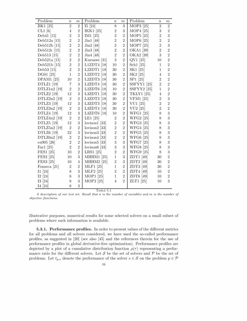
5.1. Test problems. We have collected 100 multiobjective optimization (MOO)problems reported in the literature involving only simple bounds constraints, i.e.,problems for which Ω = [ℓ, u] with ℓ, u ∈ Rn and ℓ < u. All test problems weremodeled by us in AMPL (A Modeling Language for Mathematical Programming) [22]and are available for public testing at http://www.mat.uc.pt/dms.

The problems and their dimensions are given in Table 5.1. To avoid a longpresentation we do not describe their mathematical formulations, which can be foundin the AMPL model files. We also provide in Table 5.1 the original references forthese problems — noting, however, that in some cases the formulation coded differedfrom the literature due to errors, mismatches or lack of information found in thecorresponding papers.

5.2. Solvers tested. We have considered in our numerical studies the followingpublicly available solvers for MOO without derivatives:

• AMOSA (Archived MultiObjective Simulated Annealing) [5] — www.isical.

ac.in/~sriparna_r/software.html;• BIMADS (BI-Objective Mesh Adaptive Direct Search) [3] tested only forproblems with two objective functions — www.gerad.ca/nomad/Project/

Home.html;• Epsilon-MOEA (Epsilon MultiObjective Evolutionary Algorithm) [16] — www.

iitk.ac.in/kangal/codes.shtml;• GAMULTI (Genetic Algorithms for Multiobjective, MATLAB toolbox) —www.mathworks.com;

• MOPSO (MultiObjective Particle Swarm Optimization) [8] — delta.cs.

cinvestav.mx/~ccoello/EMOO/EMOOsoftware.html;• NSGA-II (Nondominated Sorting Genetic Algorithm II, C version) [17] —www.iitk.ac.in/kangal/codes.shtml;

• NSGA-II (MATLAB implementation by A. Seshadri) — www.mathworks.

com/matlabcentral/fileexchange/10429-nsga-ii-a-multi-objective

-optimization-algorithm;• PAES (Pareto Archived Evolution Strategy) [29] — dbkgroup.org/knowles/

multi.However, in order to keep the paper to a reasonable size and not to confuse the

reader with excessive information, we are only reporting later (see Section 6.2) a partof the numerical tests that were performed. Besides five versions of our DMS, theselected solvers were AMOSA, BIMADS, and NSGA-II (C version), since these werethe ones who exhibited the best performance in the above mentioned test set. Thenumerical results regarding the remaining codes can be found in http://www.mat.

uc.pt/dms.

5.3. Metrics and profiles used for solver comparison. In the multiobjec-tive case, one is interested in assessing the ability of a solver to obtain points whichare Pareto optimal and to compute a highly diversified subset of the whole Paretofront. With these two goals in mind, we present in the next subsections the metricsused to assess the performance of the tested solvers. While there are other metricsin the literature, we have selected the ones presented herein due to their applicabilityto a large set of test problems. In particular, using a metric that considers the dis-tance from the obtained Pareto front to the true Pareto one implies the knowledgeof the latter for all the problems in the test set. In addition, presenting results for ametric that only considers a small number of test problems is meaningless. Despitenot including a metric that requires the true Pareto front, we present later, and for

15

Problem n m Problem n m Problem n mBK1 [25] 2 2 I5 [24] 8 3 MOP3 [25] 2 2CL1 [6] 4 2 IKK1 [25] 2 3 MOP4 [25] 3 2Deb41 [15] 2 2 IM1 [25] 2 2 MOP5 [25] 2 3Deb512a [15] 2 2 Jin1 [48] 2 2 MOP6 [25] 2 2Deb512b [15] 2 2 Jin2 [48] 2 2 MOP7 [25] 2 3Deb512c [15] 2 2 Jin3 [48] 2 2 OKA1 [39] 2 2Deb513 [15] 2 2 Jin4 [48] 2 2 OKA2 [39] 3 2Deb521a [15] 2 2 Kursawe [31] 3 2 QV1 [25] 10 2Deb521b [15] 2 2 L1ZDT4 [18] 10 2 Sch1 [25] 1 2Deb53 [15] 2 2 L2ZDT1 [18] 30 2 SK1 [25] 1 2DG01 [25] 1 2 L2ZDT2 [18] 30 2 SK2 [25] 4 2DPAM1 [25] 10 2 L2ZDT3 [18] 30 2 SP1 [25] 2 2DTLZ1 [19] 7 3 L2ZDT4 [18] 30 2 SSFYY1 [25] 2 2DTLZ1n2 [19] 2 2 L2ZDT6 [18] 10 2 SSFYY2 [25] 1 2DTLZ2 [19] 12 3 L3ZDT1 [18] 30 2 TKLY1 [25] 4 2DTLZ2n2 [19] 2 2 L3ZDT2 [18] 30 2 VFM1 [25] 2 3DTLZ3 [19] 12 3 L3ZDT3 [18] 30 2 VU1 [25] 2 2DTLZ3n2 [19] 2 2 L3ZDT4 [18] 30 2 VU2 [25] 2 2DTLZ4 [19] 12 3 L3ZDT6 [18] 10 2 WFG1 [25] 8 3DTLZ4n2 [19] 2 2 LE1 [25] 2 2 WFG2 [25] 8 3DTLZ5 [19] 12 3 lovison1 [33] 2 2 WFG3 [25] 8 3DTLZ5n2 [19] 2 2 lovison2 [33] 2 2 WFG4 [25] 8 3DTLZ6 [19] 22 3 lovison3 [33] 2 2 WFG5 [25] 8 3DTLZ6n2 [19] 2 2 lovison4 [33] 2 2 WFG6 [25] 8 3ex005 [26] 2 2 lovison5 [33] 3 3 WFG7 [25] 8 3Far1 [25] 2 2 lovison6 [33] 3 3 WFG8 [25] 8 3FES1 [25] 10 2 LRS1 [25] 2 2 WFG9 [25] 8 3FES2 [25] 10 3 MHHM1 [25] 1 3 ZDT1 [49] 30 2FES3 [25] 10 4 MHHM2 [25] 2 3 ZDT2 [49] 30 2Fonseca [21] 2 2 MLF1 [25] 1 2 ZDT3 [49] 30 2I1 [24] 8 3 MLF2 [25] 2 2 ZDT4 [49] 10 2I2 [24] 8 3 MOP1 [25] 1 2 ZDT6 [49] 10 2I3 [24] 8 3 MOP2 [25] 4 2 ZLT1 [25] 10 3I4 [24] 8 3

Table 5.1A description of our test set. Recall that n is the number of variables and m is the number of

objective functions.

illustrative purposes, numerical results for some selected solvers on a small subset ofproblems where such information is available.

5.3.1. Performance profiles. In order to present values of the different metricsfor all problems and all solvers considered, we have used the so-called performanceprofiles, as suggested in [20] (see also [45] and the references therein for the use ofperformance profiles in global derivative-free optimization). Performance profiles aredepicted by a plot of a cumulative distribution function ρ(τ) representing a perfor-mance ratio for the different solvers. Let S be the set of solvers and P be the set ofproblems. Let tp,s denote the performance of the solver s ∈ S on the problem p ∈ P

16

— lower values of tp,s indicate better performance. The performance ratio is definedby first setting rp,s = tp,s/mintp,s : s ∈ S, for p ∈ P and s ∈ S. Then, one definesρs(τ) = (1/|P|)|p ∈ P : rp,s ≤ τ|. Thus, the value of ρs(1) is the probability of thesolver s winning over the remaining ones. If we are only interested in determiningwhich solver is the best (in the sense of winning the most), we compare the valuesof ρs(1) for all the solvers. At the other end, solvers with the largest probabilitiesρs(τ) for large values of τ are the most robust ones (meaning the ones that solved thelargest number of problems in P).

5.3.2. Purity metric. The first metric considered by us is called Purity [4] andis used to compare the Pareto fronts obtained by different solvers. Again, let S bethe set of solvers and P be the set of problems. Let Fp,s denote the approximatedPareto front determined by the solver s ∈ S for problem p ∈ P . Let also Fp denotean approximation to the true Pareto front of problem p, calculated by first forming∪s∈SFp,s and then removing from this set any dominated points. The Purity metric

consists then in computing, for solver s ∈ S and problem p ∈ P , the ratio cFpp,s/cp,s,

where cFp

p,s = |Fp,s∩Fp| and cp,s = |Fp,s|. This metric is thus represented by a number

tp,s = cFp

p,s/cp,s between zero and one. Higher values for tp,s indicate a better Paretofront in terms of the percentage of nondominated points.

When using performance profiles to analyze the performance of the solvers mea-sured by the Purity metric, we need to set tp,s = 1/tp,s (then, again, lower values oftp,s indicate better performance). Note that when a solver s is not able to obtain asingle nondominated point in Fp, we obtain tp,s = 0, and thus tp,s = +∞, meaningthat solver s was ‘unable’ to solve problem p.

The Purity metric has shown to be sensitive to the number and type of solversconsidered in a comparison. In fact, when two ‘similar’ solvers produce similar ap-proximated Pareto fronts, their performance under the Purity metric deterioratessignificantly since many of these points will dominate each other. This effect willthen let a third solver easily win among the three. Thus, we decided to only comparesolvers in pairs when using the Purity metric. Still, since we have two solvers and alarge number of problems, we present the results using performance profiles.

An additional difficulty is the inclusion of stochastic solvers in numerical com-parisons. Since two different runs of such solvers may produce different solutions, wedecided to make 10 runs for each stochastic solver on each single problem. From these10 runs, we then selected the best and the worst run. The best run simply consistsof the run that has the higher percentage of nondominated solutions when comparedto the remaining ones (considering as a reference Pareto front the one obtained fromthe ten runs performed). In a similar way, the worst run is selected as the one withthe lowest percentage of nondominated points.

5.3.3. Spread metrics. The second type of metrics used by us tries to measurethe extent of the spread achieved in a computed Pareto front. Since we are interestedin computing a set of points that span the entire true Pareto front, the proposedmetrics have to consider first ‘extreme points’ in the objective function space Rm,which will be the same for the application of the metrics on any of the obtained fronts.The description of the computation of such ‘extreme points’ will be given later in thissubsection. We considered essentially two formulae for the spread metrics.

The first formula attempts at measuring the maximum size of the ‘holes’ of anapproximated Pareto front. Let us assume that solver s ∈ S has computed, forproblem p ∈ P , an approximated Pareto front with N points, indexed by 1, . . . , N ,

17

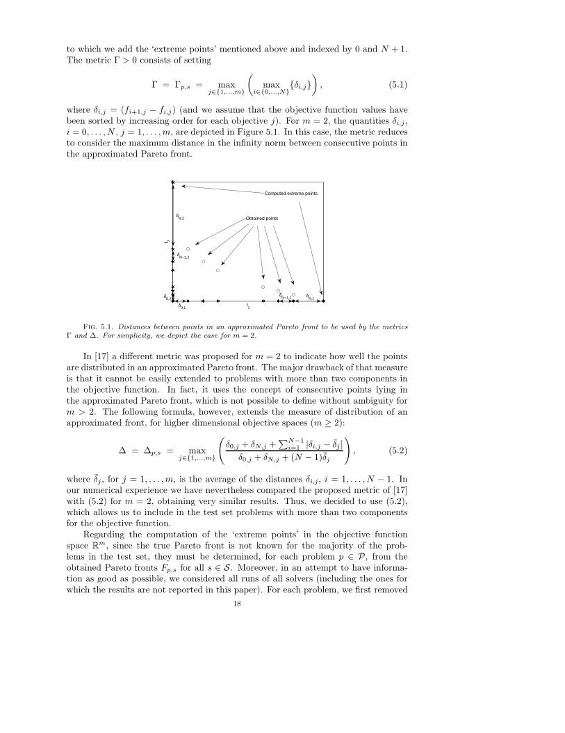
to which we add the ‘extreme points’ mentioned above and indexed by 0 and N + 1.The metric Γ > 0 consists of setting

Γ = Γp,s = maxj∈1,...,m

(

maxi∈0,...,N

δi,j

)

, (5.1)

where δi,j = (fi+1,j − fi,j) (and we assume that the objective function values havebeen sorted by increasing order for each objective j). For m = 2, the quantities δi,j ,i = 0, . . . , N , j = 1, . . . ,m, are depicted in Figure 5.1. In this case, the metric reducesto consider the maximum distance in the infinity norm between consecutive points inthe approximated Pareto front.

f1

f 2

Computed extreme points

Obtained points

δN,1

δ0,1

δ0,2

δN−1,1

δN,2

δN−1,2

Fig. 5.1. Distances between points in an approximated Pareto front to be used by the metricsΓ and ∆. For simplicity, we depict the case for m = 2.

In [17] a different metric was proposed for m = 2 to indicate how well the pointsare distributed in an approximated Pareto front. The major drawback of that measureis that it cannot be easily extended to problems with more than two components inthe objective function. In fact, it uses the concept of consecutive points lying inthe approximated Pareto front, which is not possible to define without ambiguity form > 2. The following formula, however, extends the measure of distribution of anapproximated front, for higher dimensional objective spaces (m ≥ 2):

∆ = ∆p,s = maxj∈1,...,m

(

δ0,j + δN,j +∑N−1

i=1 |δi,j − δj |

δ0,j + δN,j + (N − 1)δj

)

, (5.2)

where δj , for j = 1, . . . ,m, is the average of the distances δi,j , i = 1, . . . , N − 1. Inour numerical experience we have nevertheless compared the proposed metric of [17]with (5.2) for m = 2, obtaining very similar results. Thus, we decided to use (5.2),which allows us to include in the test set problems with more than two componentsfor the objective function.

Regarding the computation of the ‘extreme points’ in the objective functionspace Rm, since the true Pareto front is not known for the majority of the prob-lems in the test set, they must be determined, for each problem p ∈ P , from theobtained Pareto fronts Fp,s for all s ∈ S. Moreover, in an attempt to have informa-tion as good as possible, we considered all runs of all solvers (including the ones forwhich the results are not reported in this paper). For each problem, we first removed

18

the dominated points from the reunion of all these fronts. Then, for each componentof the objective function, we selected the pair corresponding to the highest pairwisedistance measured using fj(·). Note that this procedure can certainly be expensive ifwe have many points in all these fronts, but such computation can be implementedefficiently and, after all, it is part of the benchmarking and not of the optimizationitself.

We also need to use performance profiles when analyzing the results measured interms of the Γ and ∆ metrics since, again, one has the issue of having several solverson many problems. In these cases, we have set tp,s = Γp,s or tp,s = ∆p,s dependingon the metric considered.

5.3.4. Data profiles. One possible way of assessing how well derivative-freesolvers perform in terms of the number of evaluations is given by the so-called dataprofiles proposed in [37] for single objective optimization. Suppose that there is onlyone objective function f(x). For each solver, a data profile consists of a plot of thepercentage of problems that are solved for a given budget of function evaluations. Lethp,s be the number of function evaluations required for solver s ∈ S to solve problemp ∈ P (up to a certain accuracy). The data profile cumulative function is then definedby

ds(σ) =1

|P||p ∈ P : hp,s ≤ σ|. (5.3)

A critical issue related to data profiles is when a problem is considered as being solved.The authors in [37] suggested that a problem is solved (up to some level ε of accuracy)when

f(x0)− f(x) ≥ (1− ε)(f(x0)− fL), (5.4)

where x0 is the initial guess and fL is the best obtained objective function valueamong all solvers.

In the multiobjective case we need to consider instead a reference Pareto front Fp

in order to determine whether a problem p ∈ P has been solved or not. Then, asolver s is said to solve problem p, up to an accuracy of ε, if the percentage of pointsobtained in the reference Pareto front Fp is equal to or greater than 1− ε, i.e., if

|Fp,s ∩ Fp|

|Fp|/|S|≥ 1− ε, (5.5)

where Fp,s is the approximated Pareto front obtained by solver s on problem p. Notethat in (5.5) the number of points in Fp is divided by the number of solvers in S in anattempt to consider that all solvers are expected to contribute equally to the referencePareto front.

The reference Pareto front can be computed in a number of possible ways depen-ding on the choice of solvers (and on how long we let them run). To have meaningfulresults for our data profiles (in other words, a significant number of points in thenumerator of (5.5)), we considered only the solvers in the set S chosen for comparisonand a maximum number of 5000 function evaluations. The reference Pareto front isthen computed by forming the union of the output fronts of the solvers and eliminatingfrom there all the dominated points.

Following [37], we also divided σ in (5.3) by n+ 1 (the number of points neededto build a simplex gradient). Finally, note also that we did not consider any spread

19

metric for data profiles since such metrics might not decrease monotonically with thebudget σ of function evaluations (a consequence of this fact would be that a problemcould be considered unsolved after had been considered solved earlier in the runningsequence).

6. Numerical experience.

6.1. Comparing different DMS variants. The simplest possible version ofdirect multisearch (DMS), Algorithm 2.1, initializes the list of nondominated pointswith a singleton (L0 = (x0;α0)) and considers an empty search step in all iterations.This version is referred to as DMS(1). Since no initial guess has been provided alongwith the majority of the problems in our test set, it was our responsibility to definea default value for the initial point x0 to be used in DMS(1). A reasonable (perhapsthe most neutral) choice is x0 = (u+ ℓ)/2.

Since DMS is competing against population based algorithms, it is desirable toequip it with the possibility of starting from an initial list different from a singleton.Such a list can be computed by first generating a set S0 of points and then eliminatingfrom those the dominated ones. Let Snd

0 denote the resulting set. The initial list isthen given by L0 = (x;α0), x ∈ Snd

0 . We considered the three following ways ofgenerating S0 (taking |S0| = n and S0 ⊆ Ω = [ℓ, u] in all of them):

• DMS(n,line), where S0 is formed by equally spaced points on the line con-necting ℓ and u, i.e., S0 = ℓ+ (i/(n− 1))(u− ℓ), i = 0, . . . , n− 1;

• DMS(n,lhs), where S0 is generated using the Latin Hypercube Sampling strat-egy (see [35]). In this strategy, a multi-interval in Rn is partitioned into nmulti-subintervals of equal dimension and points are uniformly randomly gen-erated in each one of these multi-subintervals. The Latin Hypercube Sam-pling strategy generates random points by randomly permuting these pointsamong the multi-subintervals. Our numerical implementation uses the MAT-LAB function lhsdesign from the Statistics Toolbox, followed by a shiftingand scaling of the generated points in [0, 1]n to the multi-interval [ℓ, u];

• DMS(n,rand), where the n elements of S0 are uniformly randomly generatedin the multi-interval [ℓ, u] (see, for instance, [40]). In this case, our numericalimplementation uses the MATLAB function rand, followed by a shifting andscaling of the generated points in [0, 1]n to the multi-interval [ℓ, u].

Algorithm 2.1 allows for a variety of ways of selecting the trial list from thefiltered list. We chose to work with Algorithm 2.3, meaning that Ltrial = Lfiltered.The strategy chosen to manage the list consisted of always add points to the end ofthe list and move a point already selected as a poll center to the end of the list (atthe end of an iteration).

For all the variants tested (DMS(1), DMS(n,line), DMS(n,lhs), and DMS(n,rand)),we chose1 Dk = [In − In], where In is the identity matrix of order n. We have cho-sen ρ(·) as the constant, zero vector of dimension m. The step size parameter washalved in unsuccessful iterations and maintained in successful ones. Note that sincethe search step is empty these choices respect the requirements for global convergenceby integer lattices (see Section A.1).

Also, for all variants, we picked α0 = 1 and adopted a stopping criterion consisting

1It is important to note that the result of Theorem 4.9 was derived under the assumption thatthe set of refining directions was dense in the unit sphere. We also tried in our numerical setting touse a poll set Dk equal to [Qk − Qk] (where Qk is an orthogonal matrix computed by randomlygenerating the first column) but the results were not better.

20

0.5 1 1.5 2 2.5 30

0.1

0.2

0.3

0.4

0.5

0.6

0.7

0.8

0.9

1Purity performance profile

τ

ρ

DMS(1)DMS(n,line)

5 10 15 20 250

0.1

0.2

0.3

0.4

0.5

0.6

0.7

0.8

0.9

1

τ

ρ

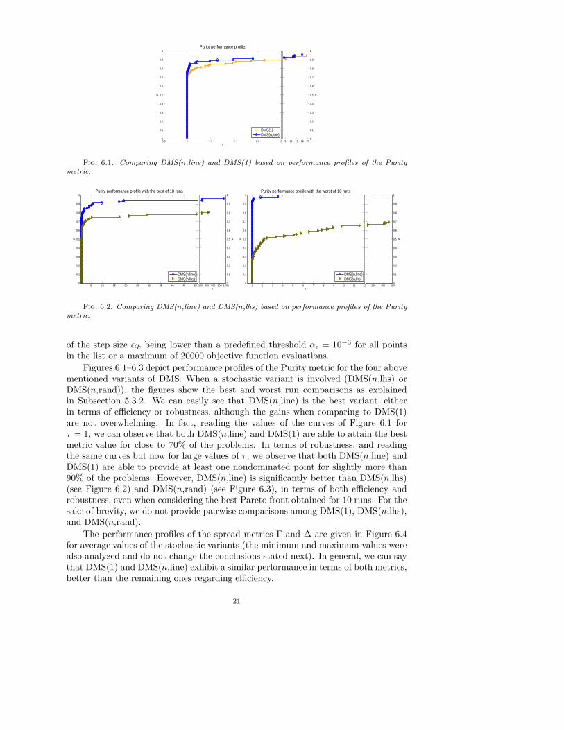
Fig. 6.1. Comparing DMS(n,line) and DMS(1) based on performance profiles of the Puritymetric.

5 10 15 20 25 30 35 40 45 500

0.1

0.2

0.3

0.4

0.5

0.6

0.7

0.8

0.9

1Purity performance profile with the best of 10 runs

τ

ρ

DMS(n,line)DMS(n,lhs)

200 400 600 800 10000

0.1

0.2

0.3

0.4

0.5

0.6

0.7

0.8

0.9

1

τ

ρ

1 2 3 4 5 6 7 8 9 10 11 120

0.1

0.2

0.3

0.4

0.5

0.6

0.7

0.8

0.9

1Purity performance profile with the worst of 10 runs

τ

ρ

DMS(n,line)DMS(n,lhs)

200 400 6000

0.1

0.2

0.3

0.4

0.5

0.6

0.7

0.8

0.9

1

τ

ρ

Fig. 6.2. Comparing DMS(n,line) and DMS(n,lhs) based on performance profiles of the Puritymetric.

of the step size αk being lower than a predefined threshold αǫ = 10−3 for all pointsin the list or a maximum of 20000 objective function evaluations.

Figures 6.1–6.3 depict performance profiles of the Purity metric for the four abovementioned variants of DMS. When a stochastic variant is involved (DMS(n,lhs) orDMS(n,rand)), the figures show the best and worst run comparisons as explainedin Subsection 5.3.2. We can easily see that DMS(n,line) is the best variant, eitherin terms of efficiency or robustness, although the gains when comparing to DMS(1)are not overwhelming. In fact, reading the values of the curves of Figure 6.1 forτ = 1, we can observe that both DMS(n,line) and DMS(1) are able to attain the bestmetric value for close to 70% of the problems. In terms of robustness, and readingthe same curves but now for large values of τ , we observe that both DMS(n,line) andDMS(1) are able to provide at least one nondominated point for slightly more than90% of the problems. However, DMS(n,line) is significantly better than DMS(n,lhs)(see Figure 6.2) and DMS(n,rand) (see Figure 6.3), in terms of both efficiency androbustness, even when considering the best Pareto front obtained for 10 runs. For thesake of brevity, we do not provide pairwise comparisons among DMS(1), DMS(n,lhs),and DMS(n,rand).

The performance profiles of the spread metrics Γ and ∆ are given in Figure 6.4for average values of the stochastic variants (the minimum and maximum values werealso analyzed and do not change the conclusions stated next). In general, we can saythat DMS(1) and DMS(n,line) exhibit a similar performance in terms of both metrics,better than the remaining ones regarding efficiency.

21

5 10 15 20 25 30 35 400

0.1

0.2

0.3

0.4

0.5

0.6

0.7

0.8

0.9


τ

ρ

DMS(n,line)DMS(n,rand)

200 300 400 5000

0.1

0.2

0.3

0.4

0.5

0.6

0.7

0.8

0.9

1

τ

ρ

10 20 30 40 50 60 700

0.1

0.2

0.3

0.4

0.5

0.6

0.7

0.8

0.9


τ

ρ

DMS(n,line)DMS(n,rand)

800 1000 1200 14000

0.1

0.2

0.3

0.4

0.5

0.6

0.7

0.8

0.9

1

τ

ρ

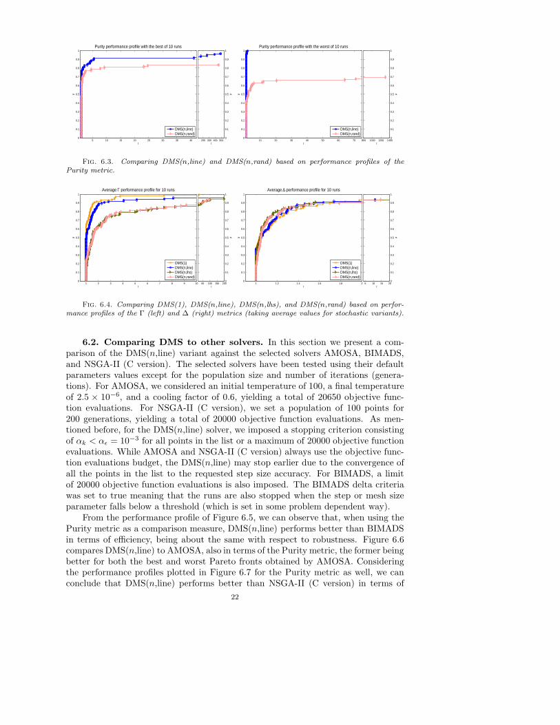
Fig. 6.3. Comparing DMS(n,line) and DMS(n,rand) based on performance profiles of thePurity metric.

1 2 3 4 5 6 7 8 9 100

0.1

0.2

0.3

0.4

0.5

0.6

0.7

0.8

0.9

1Average Γ performance profile for 10 runs

τ

ρ

DMS(1)DMS(n,line)DMS(n,lhs)DMS(n,rand)

50 100 150 2000

0.1

0.2

0.3

0.4

0.5

0.6

0.7

0.8

0.9

1

τ

ρ

1 1.2 1.4 1.6 1.8 20

0.1

0.2

0.3

0.4

0.5

0.6

0.7

0.8

0.9

1Average ∆ performance profile for 10 runs

τ

ρ

DMS(1)DMS(n,line)DMS(n,lhs)DMS(n,rand)

5 10 15 200

0.1

0.2

0.3

0.4

0.5

0.6

0.7

0.8

0.9

1

τ

ρ

Fig. 6.4. Comparing DMS(1), DMS(n,line), DMS(n,lhs), and DMS(n,rand) based on perfor-mance profiles of the Γ (left) and ∆ (right) metrics (taking average values for stochastic variants).

6.2. Comparing DMS to other solvers. In this section we present a com-parison of the DMS(n,line) variant against the selected solvers AMOSA, BIMADS,and NSGA-II (C version). The selected solvers have been tested using their defaultparameters values except for the population size and number of iterations (genera-tions). For AMOSA, we considered an initial temperature of 100, a final temperatureof 2.5 × 10−6, and a cooling factor of 0.6, yielding a total of 20650 objective func-tion evaluations. For NSGA-II (C version), we set a population of 100 points for200 generations, yielding a total of 20000 objective function evaluations. As men-tioned before, for the DMS(n,line) solver, we imposed a stopping criterion consistingof αk < αǫ = 10−3 for all points in the list or a maximum of 20000 objective functionevaluations. While AMOSA and NSGA-II (C version) always use the objective func-tion evaluations budget, the DMS(n,line) may stop earlier due to the convergence ofall the points in the list to the requested step size accuracy. For BIMADS, a limitof 20000 objective function evaluations is also imposed. The BIMADS delta criteriawas set to true meaning that the runs are also stopped when the step or mesh sizeparameter falls below a threshold (which is set in some problem dependent way).

From the performance profile of Figure 6.5, we can observe that, when using thePurity metric as a comparison measure, DMS(n,line) performs better than BIMADSin terms of efficiency, being about the same with respect to robustness. Figure 6.6compares DMS(n,line) to AMOSA, also in terms of the Purity metric, the former beingbetter for both the best and worst Pareto fronts obtained by AMOSA. Consideringthe performance profiles plotted in Figure 6.7 for the Purity metric as well, we canconclude that DMS(n,line) performs better than NSGA-II (C version) in terms of

22

1 1.5 2 2.5 3 3.5 4 4.5 5 5.50

0.1

0.2

0.3

0.4

0.5

0.6

0.7

0.8

0.9


τ

ρ

DMS(n,line)BIMADS

Fig. 6.5. Comparing DMS(n,line) and BIMADS based on performance profiles of the Puritymetric (only problems with two objective functions were considered).

10 20 30 40 50 60 70 80 90 100 1100

0.1

0.2

0.3

0.4

0.5

0.6

0.7

0.8

0.9


τ

ρ

DMS(n,line)AMOSA

200 400 600 800 10000

0.1

0.2

0.3

0.4

0.5

0.6

0.7

0.8

0.9

1

τ

ρ

10 20 30 40 50 60 70 80 90 100 1100

0.1

0.2

0.3

0.4

0.5

0.6

0.7

0.8

0.9


τ

ρ

DMS(n,line)AMOSA

200 400 600 800 10000

0.1

0.2

0.3

0.4

0.5

0.6

0.7

0.8

0.9

1

τ

ρ

Fig. 6.6. Comparing DMS(n,line) and AMOSA based on performance profiles of the Puritymetric.

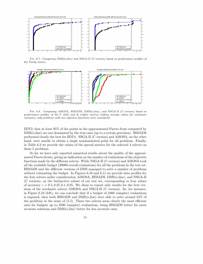
efficiency. Regarding robustness, and also looking at Figure 6.7, DMS(n,line) slightlyoutperforms NSGA-II (C version) when considering its worst Pareto front, and slightlylooses compared to its best Pareto front.

Figure 6.8 depicts the performance profiles using the spread metrics Γ and ∆(see (5.1) and (5.2)) for problems where m = 2 (again we only show the results foraverage values of the stochastic variants as the ones for minimum and maximumvalues do not affect our conclusions). One can observe that DMS(n,line) exhibits thebest overall performance for the Γ matric, although NSGA-II (C version) is slightlymore efficient in terms of the ∆ metric. Such conclusions are true mainly in terms ofefficiency, since the four solvers seem to be equally robust under both metrics. Theseconclusions are also supported from the performance profiles of Figure 6.9 where allthe problems are considered (m ≥ 2) and BIMADS is excluded due to its limitationto m = 2.

As previously mentioned, we did not use any metric which required the knowledgeof the true Pareto front. This set is known, however, for some of the problems, suchas Problems ZDT1–ZDT4 and ZDT6 (and is discontinuous for ZDT3).

When the true Pareto front is known, which is the case for these five problems (seehttp://www.tik.ee.ethz.ch/sop/download/supplementary/testproblems), onecan also use the Purity metric to compare the approximated Pareto fronts to thetrue one. Table 6.1 presents such results for the 5 problems under consideration.There are analytical expressions for the Pareto fronts of these problems, where f2 isgiven in terms of f1. We considered discretized forms of these fronts by letting f1vary in a equally spaced grid of step 10−5. One can see, for problems ZDT1 and

23

0.5 1 1.5 2 2.5 3 3.5 4 4.5 50

0.1

0.2

0.3

0.4

0.5

0.6

0.7

0.8

0.9


τ

ρ

DMS(n,line)NSGA−II (C version)

20 40 600

0.1

0.2

0.3

0.4

0.5

0.6

0.7

0.8

0.9

1

τ

ρ

0.5 1 1.5 2 2.5 3 3.50

0.1

0.2

0.3

0.4

0.5

0.6

0.7

0.8

0.9


τ

ρ

DMS(n,line)NSGA−II (C version)

10 20 300

0.1

0.2

0.3

0.4

0.5

0.6

0.7

0.8

0.9

1

τ

ρ

Fig. 6.7. Comparing DMS(n,line) and NSGA-II (C version) based on performance profiles ofthe Purity metric.

50 100 150 200 2500

0.1

0.2

0.3

0.4

0.5

0.6

0.7

0.8

0.9


τ

ρ

DMS(n,line)BIMADSNSGA−II (C version)AMOSA

500 1000 1500 20000

0.1

0.2

0.3

0.4

0.5

0.6

0.7

0.8

0.9

1

τ

ρ

0.5 1 1.5 2 2.5 3 3.5 4 4.5 5 5.5 60

0.1

0.2

0.3

0.4

0.5

0.6

0.7

0.8

0.9


τ

ρ


1000 2000 30000

0.1

0.2

0.3

0.4

0.5

0.6

0.7

0.8

0.9

1

τ

ρ

Fig. 6.8. Comparing AMOSA, BIMADS, DMS(n,line), and NSGA-II (C version) based onperformance profiles of the Γ (left) and ∆ (right) metrics (taking average values for stochasticvariants); only problems with two objective functions were considered.

ZDT2, that at least 95% of the points in the approximated Pareto front computed byDMS(n,line) are not dominated by the true ones (up to a certain precision). BIMADSperformed clearly the best for ZDT4. NSGA-II (C version) and AMOSA, on the otherhand, were unable to obtain a single nondominated point for all problems. Finally,in Table 6.2 we provide the values of the spread metrics for the selected 4 solvers onthese 5 problems.

So far we have only reported numerical results about the quality of the approxi-mated Pareto fronts, giving no indication on the number of evaluations of the objectivefunctions made by the different solvers. While NSGA-II (C version) and AMOSA tookall the available budget (20000 overall evaluations) for all the problems in the test set,BIMADS and the different versions of DMS managed to solve a number of problemswithout exhausting the budget. In Figures 6.10 and 6.11 we provide data profiles forthe four solvers under consideration, AMOSA, BIMADS, DMS(n,line), and NSGA-II(C version), on the biobjective subset of our test set, corresponding to four valuesof accuracy ε = 0.5, 0.25, 0.1, 0.05. We chose to report only results for the best ver-sions of the stochastic solvers AMOSA and NSGA-II (C version). So, for instance,in Figure 6.10 (left), we can conclude that if a budget of 1000 (simplex) evaluationsis imposed, then both BIMADS and DMS(n,line) were able to solve around 54% ofthe problems in the sense of (5.5). These two solvers seem clearly the most efficientones for budgets up to 2500 (simplex) evaluations, being BIMADS better for moreaccurate solutions and DMS(n,line) better for less accurate ones.

24

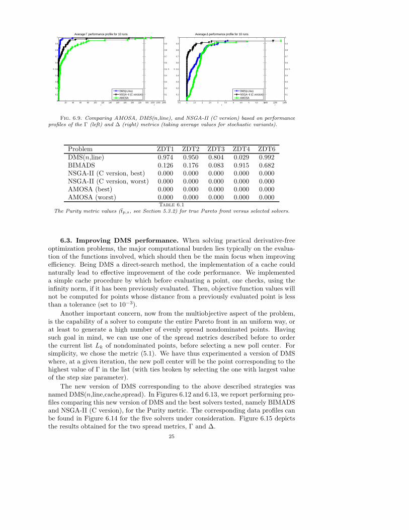
20 40 60 80 100 120 140 160 180 200 2200

0.1

0.2

0.3

0.4

0.5

0.6

0.7

0.8

0.9


τ

ρ

DMS(n,line)NSGA−II (C version)AMOSA

500 1000 1500 20000

0.1

0.2

0.3

0.4

0.5

0.6

0.7

0.8

0.9

1

τ

ρ

0.5 1 1.5 2 2.5 3 3.5 4 4.5 5 5.5 60

0.1

0.2

0.3

0.4

0.5

0.6

0.7

0.8

0.9


τ

ρ

DMS(n,line)NSGA−II (C version)AMOSA

1000 1200 14000

0.1

0.2

0.3

0.4

0.5

0.6

0.7

0.8

0.9

1

τ

ρ

Fig. 6.9. Comparing AMOSA, DMS(n,line), and NSGA-II (C version) based on performanceprofiles of the Γ (left) and ∆ (right) metrics (taking average values for stochastic variants).

Problem ZDT1 ZDT2 ZDT3 ZDT4 ZDT6DMS(n,line) 0.974 0.950 0.804 0.029 0.992BIMADS 0.126 0.176 0.083 0.915 0.682NSGA-II (C version, best) 0.000 0.000 0.000 0.000 0.000NSGA-II (C version, worst) 0.000 0.000 0.000 0.000 0.000AMOSA (best) 0.000 0.000 0.000 0.000 0.000AMOSA (worst) 0.000 0.000 0.000 0.000 0.000

Table 6.1The Purity metric values (tp,s, see Section 5.3.2) for true Pareto front versus selected solvers.

6.3. Improving DMS performance. When solving practical derivative-freeoptimization problems, the major computational burden lies typically on the evalua-tion of the functions involved, which should then be the main focus when improvingefficiency. Being DMS a direct-search method, the implementation of a cache couldnaturally lead to effective improvement of the code performance. We implementeda simple cache procedure by which before evaluating a point, one checks, using theinfinity norm, if it has been previously evaluated. Then, objective function values willnot be computed for points whose distance from a previously evaluated point is lessthan a tolerance (set to 10−3).

Another important concern, now from the multiobjective aspect of the problem,is the capability of a solver to compute the entire Pareto front in an uniform way, orat least to generate a high number of evenly spread nondominated points. Havingsuch goal in mind, we can use one of the spread metrics described before to orderthe current list Lk of nondominated points, before selecting a new poll center. Forsimplicity, we chose the metric (5.1). We have thus experimented a version of DMSwhere, at a given iteration, the new poll center will be the point corresponding to thehighest value of Γ in the list (with ties broken by selecting the one with largest valueof the step size parameter).

The new version of DMS corresponding to the above described strategies wasnamed DMS(n,line,cache,spread). In Figures 6.12 and 6.13, we report performing pro-files comparing this new version of DMS and the best solvers tested, namely BIMADSand NSGA-II (C version), for the Purity metric. The corresponding data profiles canbe found in Figure 6.14 for the five solvers under consideration. Figure 6.15 depictsthe results obtained for the two spread metrics, Γ and ∆.

25

Problem ZDT1 ZDT2 ZDT3 ZDT4 ZDT6Γ

DMS(n,line) 0.044 0.010 0.537 0.125 3.808BIMADS 0.040 0.035 0.197 0.145 1.791NSGA-II (C version) 0.053 0.161 0.172 7.135 1.894AMOSA 0.240 0.122 0.186 0.094 1.652

∆DMS(n,line) 0.555 0.492 1.464 0.696 1.184BIMADS 1.378 1.389 1.604 1.942 1.313NSGA-II (C version) 0.660 0.788 1.326 0.986 0.998AMOSA 0.800 0.795 1.284 0.915 1.287

Table 6.2The Γ and ∆ metrics values for the selected solvers. (Only average values are provided for

stochastic solvers.)

0 500 1000 1500 2000 25000

0.1

0.2

0.3

0.4

0.5

0.6

0.7

0.8

0.9

1Data profile with the best of 10 runs (ε=0.5)

σ

d s(σ)


0 500 1000 1500 20000

0.1

0.2

0.3

0.4

0.5

0.6

0.7

0.8

0.9


σ

d s(σ)


Fig. 6.10. Data profiles for AMOSA, BIMADS, DMS(n,line), and NSGA-II (C version) solvers(ε = 0.5 on the left and ε = 0.25 on the right).

From the observation of these profiles, we can conclude that the modificationsconsidered, implemented in the variant DMS(n,line,cache,spread), led to an even fur-ther improving of the efficiency and robustness of the basic DMS algorithm.

7. Conclusions. In this paper we introduced, analyzed, and tested a new algo-rithmic approach for multiobjective optimization (MOO) without derivatives. Thisapproach has been called direct multisearch (DMS) since it naturally generalizes directsearch (of directional type) from single to multiobjective optimization. The principlesof DMS are extremely simple. Instead of updating a single point per iteration, it up-dates an iterate list of feasible nondominated points. Iteration success is measured bychanges in the iterate list. Each iteration of DMS includes provision for an optionalsearch step. Polling is also applied, as in single objective optimization, at a selectedpoint of the iterate list. Both steps can add points to the iterate list, forming a filteredintermediate list, and there is significant flexibility in the way a trial list is formedfrom this filtered list.

The goal of DMS is to approximate the true (global, if possible) Pareto front,although theoretically one is only able to prove that there is a limit point in a sta-tionary form of this front, as no aggregation or scalarization technique is incorporatedin DMS. For this purpose, and to be able to state results for nonsmooth objectivefunctions, we used in this paper the notion of a Clarke-Pareto stationary or critical

26

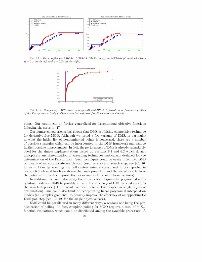
0 500 1000 1500 2000 25000

0.1

0.2

0.3

0.4

0.5

0.6

0.7

0.8

0.9


σ

d s(σ)


0 500 1000 1500 2000 25000

0.1

0.2

0.3

0.4

0.5

0.6

0.7

0.8

0.9


σ

d s(σ)


Fig. 6.11. Data profiles for AMOSA, BIMADS, DMS(n,line), and NSGA-II (C version) solvers(ε = 0.1 on the left and ε = 0.05 on the right).

0.5 1 1.5 2 2.5 3 3.5 4 4.50

0.1

0.2

0.3

0.4

0.5

0.6

0.7

0.8

0.9


τ

ρ

DMS(n,line,cache,spread)BIMADS

Fig. 6.12. Comparing DMS(n,line,cache,spread) and BIMADS based on performance profilesof the Purity metric (only problems with two objective functions were considered).

point. Our results can be further generalized for discontinuous objective functionsfollowing the steps in [47].

Our numerical experience has shown that DMS is a highly competitive techniquefor derivative-free MOO. Although we tested a few variants of DMS, in particularin what the initial list of nondominated points is concerned, there are a numberof possible strategies which can be incorporated in the DMS framework and lead tofurther possible improvements. In fact, the performance of DMS is already remarkablygood for the simple implementations tested on Sections 6.1 and 6.2 which do notincorporate any dissemination or spreading techniques particularly designed for thedetermination of the Pareto front. Such techniques could be easily fitted into DMSby means of an appropriate search step (such as a swarm search step; see [45, 46]for m = 1) or by selecting the poll centers using a spread metric (as reported inSection 6.3 where it has been shown that such procedure and the use of a cache havethe potential to further improve the performance of the more basic versions).

In addition, one could also study the introduction of quadratic polynomial inter-polation models in DMS to possibly improve the efficiency of DMS in what concernsthe search step (see [11] for what has been done in this respect in single objectiveoptimization). One could also think of incorporating linear polynomial interpolationmodels (i.e., simplex gradients) to possibly improve the efficiency of an opportunisticDMS poll step (see [10, 12] for the single objective case).

DMS could be parallelized in many different ways, a obvious one being the par-allelization of polling. In fact, complete polling for MOO requires a total of m|Dk|function evaluations, which could be distributed among the available processors. A

27

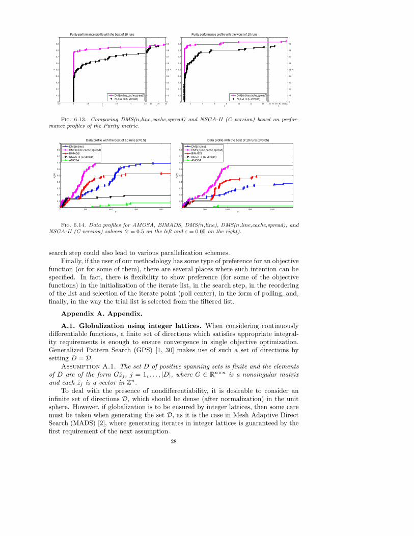
0.5 1 1.5 2 2.5 3 3.50

0.1

0.2

0.3

0.4

0.5

0.6

0.7

0.8

0.9


τ

ρ

DMS(n,line,cache,spread)NSGA−II (C version)

10 20 300

0.1

0.2

0.3

0.4

0.5

0.6

0.7

0.8

0.9

1

τ

ρ

2 4 6 8 10 12 140

0.1

0.2

0.3

0.4

0.5

0.6

0.7

0.8

0.9


τ

ρ

DMS(n,line,cache,spread)NSGA−II (C version)

20 40 60 80 100 1200

0.1

0.2

0.3

0.4

0.5

0.6

0.7

0.8

0.9

1

τ

ρ

Fig. 6.13. Comparing DMS(n,line,cache,spread) and NSGA-II (C version) based on perfor-mance profiles of the Purity metric.

0 500 1000 1500 20000

0.1

0.2

0.3

0.4

0.5

0.6

0.7

0.8

0.9


σ

d s(σ)

DMS(n,line)DMS(n,line,cache,spread)BIMADSNSGA−II (C version)AMOSA

0 500 1000 1500 20000

0.1

0.2

0.3

0.4

0.5

0.6

0.7

0.8

0.9


σ

d s(σ)


Fig. 6.14. Data profiles for AMOSA, BIMADS, DMS(n,line), DMS(n,line,cache,spread), andNSGA-II (C version) solvers (ε = 0.5 on the left and ε = 0.05 on the right).

search step could also lead to various parallelization schemes.Finally, if the user of our methodology has some type of preference for an objective

function (or for some of them), there are several places where such intention can bespecified. In fact, there is flexibility to show preference (for some of the objectivefunctions) in the initialization of the iterate list, in the search step, in the reorderingof the list and selection of the iterate point (poll center), in the form of polling, and,finally, in the way the trial list is selected from the filtered list.

Appendix A. Appendix.

A.1. Globalization using integer lattices. When considering continuouslydifferentiable functions, a finite set of directions which satisfies appropriate integral-ity requirements is enough to ensure convergence in single objective optimization.Generalized Pattern Search (GPS) [1, 30] makes use of such a set of directions bysetting D = D.

Assumption A.1. The set D of positive spanning sets is finite and the elementsof D are of the form Gzj, j = 1, . . . , |D|, where G ∈ Rn×n is a nonsingular matrixand each zj is a vector in Zn.

To deal with the presence of nondifferentiability, it is desirable to consider aninfinite set of directions D, which should be dense (after normalization) in the unitsphere. However, if globalization is to be ensured by integer lattices, then some caremust be taken when generating the set D, as it is the case in Mesh Adaptive DirectSearch (MADS) [2], where generating iterates in integer lattices is guaranteed by thefirst requirement of the next assumption.

28

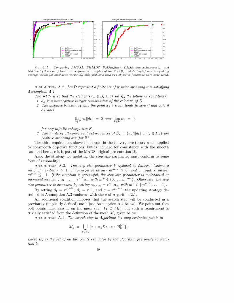
50 100 150 200 2500

0.1

0.2

0.3

0.4

0.5

0.6

0.7

0.8

0.9


τ

ρ


500 1000 1500 20000

0.1

0.2

0.3

0.4

0.5

0.6

0.7

0.8

0.9

1

τ

ρ

0.5 1 1.5 2 2.5 3 3.5 4 4.5 5 5.50

0.1

0.2

0.3

0.4

0.5

0.6

0.7

0.8

0.9


τ

ρ


1000 2000 30000

0.1

0.2

0.3

0.4

0.5

0.6

0.7

0.8

0.9

1

τ

ρ

Fig. 6.15. Comparing AMOSA, BIMADS, DMS(n,line), DMS(n,line,cache,spread), andNSGA-II (C version) based on performance profiles of the Γ (left) and ∆ (right) metrics (takingaverage values for stochastic variants); only problems with two objective functions were considered.

Assumption A.2. Let D represent a finite set of positive spanning sets satisfyingAssumption A.1.

The set D is so that the elements dk ∈ Dk ⊆ D satisfy the following conditions:1. dk is a nonnegative integer combination of the columns of D.2. The distance between xk and the point xk + αkdk tends to zero if and only if

αk does:

limk∈K

αk‖dk‖ = 0 ⇐⇒ limk∈K

αk = 0,

for any infinite subsequence K.3. The limits of all convergent subsequences of Dk = dk/‖dk‖ : dk ∈ Dk are

positive spanning sets for Rn.The third requirement above is not used in the convergence theory when applied

to nonsmooth objective functions, but is included for consistency with the smoothcase and because it is part of the MADS original presentation [2].

Also, the strategy for updating the step size parameter must conform to someform of rationality.

Assumption A.3. The step size parameter is updated as follows: Choose arational number τ > 1, a nonnegative integer mmax ≥ 0, and a negative integermmin ≤ −1. If the iteration is successful, the step size parameter is maintained orincreased by taking αk,new = τm

+

αk, with m+ ∈ 0, . . . ,mmax. Otherwise, the step

size parameter is decreased by setting αk,new = τm−

αk, with m− ∈ mmin, . . . ,−1.

By setting β1 = τmmin

, β2 = τ−1, and γ = τmmax

, the updating strategy de-scribed in Assumption A.3 conforms with those of Algorithm 2.1.

An additional condition imposes that the search step will be conducted in apreviously (implicitly defined) mesh (see Assumption A.4 below). We point out thatpoll points must also lie on the mesh (i.e., Pk ⊂ Mk), but such a requirement istrivially satisfied from the definition of the mesh Mk given below.

Assumption A.4. The search step in Algorithm 2.1 only evaluates points in

Mk =⋃

x∈Ek

x+ αkDz : z ∈ N|D|0 ,

where Ek is the set of all the points evaluated by the algorithm previously to itera-tion k.

29

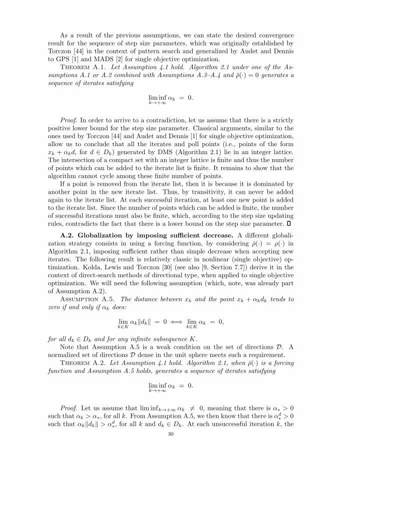
As a result of the previous assumptions, we can state the desired convergenceresult for the sequence of step size parameters, which was originally established byTorczon [44] in the context of pattern search and generalized by Audet and Dennisto GPS [1] and MADS [2] for single objective optimization.

Theorem A.1. Let Assumption 4.1 hold. Algorithm 2.1 under one of the As-sumptions A.1 or A.2 combined with Assumptions A.3–A.4 and ρ(·) = 0 generates asequence of iterates satisfying

lim infk→+∞

αk = 0.

Proof. In order to arrive to a contradiction, let us assume that there is a strictlypositive lower bound for the step size parameter. Classical arguments, similar to theones used by Torczon [44] and Audet and Dennis [1] for single objective optimization,allow us to conclude that all the iterates and poll points (i.e., points of the formxk + αkd, for d ∈ Dk) generated by DMS (Algorithm 2.1) lie in an integer lattice.The intersection of a compact set with an integer lattice is finite and thus the numberof points which can be added to the iterate list is finite. It remains to show that thealgorithm cannot cycle among these finite number of points.

If a point is removed from the iterate list, then it is because it is dominated byanother point in the new iterate list. Thus, by transitivity, it can never be addedagain to the iterate list. At each successful iteration, at least one new point is addedto the iterate list. Since the number of points which can be added is finite, the numberof successful iterations must also be finite, which, according to the step size updatingrules, contradicts the fact that there is a lower bound on the step size parameter.

A.2. Globalization by imposing sufficient decrease. A different globali-zation strategy consists in using a forcing function, by considering ρ(·) = ρ(·) inAlgorithm 2.1, imposing sufficient rather than simple decrease when accepting newiterates. The following result is relatively classic in nonlinear (single objective) op-timization. Kolda, Lewis and Torczon [30] (see also [9, Section 7.7]) derive it in thecontext of direct-search methods of directional type, when applied to single objectiveoptimization. We will need the following assumption (which, note, was already partof Assumption A.2).

Assumption A.5. The distance between xk and the point xk + αkdk tends tozero if and only if αk does:

limk∈K

αk‖dk‖ = 0 ⇐⇒ limk∈K

αk = 0,

for all dk ∈ Dk and for any infinite subsequence K.Note that Assumption A.5 is a weak condition on the set of directions D. A

normalized set of directions D dense in the unit sphere meets such a requirement.Theorem A.2. Let Assumption 4.1 hold. Algorithm 2.1, when ρ(·) is a forcing

function and Assumption A.5 holds, generates a sequence of iterates satisfying

lim infk→+∞

αk = 0.

Proof. Let us assume that lim infk→+∞ αk 6= 0, meaning that there is α∗ > 0such that αk > α∗, for all k. From Assumption A.5, we then know that there is αd

∗ > 0such that αk‖dk‖ > αd

∗, for all k and dk ∈ Dk. At each unsuccessful iteration k, the

30

corresponding step size parameter is reduced by at least β2 ∈ (0, 1), and thus thenumber of successful iterations must be infinite. Since ρ(·) is a non decreasing function,which satisfies ρ(t) > 0, for t > 0, there exists ρ∗ > 0 such that ρ(αk) ≥ ρ(α∗) ≥ ρ∗and ρ(αk‖dk‖) ≥ ρ(αd

∗) ≥ ρ∗, for all k and dk ∈ Dk, with ρ∗ = min(ρ(α∗), ρ(αd∗)),

taking into account what can happen in both the search and the poll steps.At each successful iteration, any new point added to the current iterate list will

define a hypercube of length no smaller than ρ∗ in the set of points nondominatedby those in the iterate list, where it will be later impossible to generate a new point.This and the fact that the number of successful iterations is infinite contradict As-sumption 4.1.

Acknowledgments. The authors would like to thank John Dennis (Rice Uni-versity) and Jorg Fliege (University of Southampton) for interesting discussions onderivative-free multiobjective optimization. We are also grateful to two anonymousreferees whose comments much improved the presentation of the paper.

REFERENCES

[1] C. Audet and J. E. Dennis Jr., Analysis of generalized pattern searches, SIAM J. Optim., 13(2002), pp. 889–903.

[2] , Mesh adaptive direct search algorithms for constrained optimization, SIAM J. Optim.,17 (2006), pp. 188–217.

[3] C. Audet, G. Savard, and W. Zghal, Multiobjective optimization through a series of single-objective formulations, SIAM J. Optim., 19 (2008), pp. 188–210.

[4] S. Bandyopadhyay, S. K. Pal, and B. Aruna, Multiobjective GAs, quantative indices, andpattern classification, IEEE Transactions on Systems, Man, and Cybernetics – Part B:Cybernetics, 34 (2004), pp. 2088–2099.

[5] S. Bandyopadhyay, S. Saha, U. Maulik, and K. Deb, A simulated anneling-based multiobjec-tive optimization algorithm: AMOSA, IEEE Transactions on Evolutionary Computation,12 (2008), pp. 269–283.

[6] F. Y. Cheng and X. S. Li, Generalized center method for multiobjective engineering optimiza-tion, Engineering Optimization, 31 (1999), pp. 641–661.

[7] F. H. Clarke, Optimization and Nonsmooth Analysis, John Wiley & Sons, New York, 1983.Reissued by SIAM, Philadelphia, 1990.

[8] C. A. Coello Coello and M. S. Lechuga, Mopso: A proposal for multiple objective particleswarm optimization, in Congress on Evolutionary Computation (CEC’2002), vol. 2, LosAlamitos,USA, 2002, IEEE Computer Society, pp. 1051–1056.

[9] A. R. Conn, K. Scheinberg, and L. N. Vicente, Introduction to Derivative-Free Optimiza-tion, MPS-SIAM Series on Optimization, SIAM, Philadelphia, 2009.

[10] A. L. Custodio, J. E. Dennis Jr., and L. N. Vicente, Using simplex gradients of nonsmoothfunctions in direct search methods, IMA J. Numer. Anal., 28 (2008), pp. 770–784.

[11] A. L. Custodio, H. Rocha, and L. N. Vicente, Incorporating minimum Frobenius normmodels in direct search, Comput. Optim. Appl., 46 (2010), pp. 265–278.

[12] A. L. Custodio and L. N. Vicente, Using sampling and simplex derivatives in pattern searchmethods, SIAM J. Optim., 18 (2007), pp. 537–555.

[13] I. Das and J. E. Dennis, A closer look at drawbacks of minimizing weighted sums of objec-tives for pareto set generation in multicriteria optimization problems, Struct. Multidiscip.Optim., 14 (1997), pp. 63–69.

[14] I. Das and J. E. Dennis Jr., Normal-boundary intersection: a new method for generating thepareto surface in nonlinear multicriteria optimization problems, SIAM J. Optim., 8 (1998),pp. 631–657.

[15] K. Deb, Multi-objective genetic algorithms: Problem difficulties and construction of test prob-lems, Evolutionary Computation, 7 (1999), pp. 205–230.

31

[16] K. Deb, M. Mohan, and S. Mishra, Towards a quick computation of well-spread pareto-optimal solutions, in Evolutionary Multi-Criterion Optimization (EMO 2003), C. Fonsecaet al., ed., vol. 2632 of Lecture Notes in Computer Science, 2003, pp. 222–236.

[17] K. Deb, A. Pratap, S. Agarwal, and T. Meyarivan, A fast and elitist multiobjective geneticalgorithm: NSGA-II, IEEE Transactions on Evolutionary Computation, 6 (2002), pp. 182–197.

[18] K. Deb, A. Sinha, and S. Kukkonen, Multi-objective test problems, linkages, and evolutionarymethodologies, in Proceedings of the 8th Annual Conference on Genetic and EvolutionaryComputation GECCO’06, New York, USA, 2006, ACM, pp. 1141–1148.

[19] K. Deb, L. Thiele, M. Laumanns, and E. Zitzler, Scalable multi-objective optimization testproblems, in Proceedings of the Congress on Evolutionary Computation (CEC’02), vol. 1,Honolulu, HI, 2002, IEEE Press, pp. 825–830.

[20] E. D. Dolan and J. J. More, Benchmarking optimization software with performance profiles,Math. Program., 91 (2002), pp. 201–213.

[21] C. M. Fonseca and P. J. Fleming, Multiobjective optimization and multiple constraint han-dling with evolutionary algorithms – Part I: A unified formulation, IEEE Transactions onSystems, Man, and Cybernetics – Part A: Systems and Humans, 28 (1998), pp. 26–37.

[22] R. Fourer, D. M. Gay, and B. W. Kernighan, A modeling language for mathematical pro-gramming, Management Sci., 36 (1990), pp. 519–554.

[23] A. L. Hoffmann, A. Y. D. Siem, D. den Hertog, J. H. A. M. Kaanders, and H. Huizenga,Derivative-free generation and interpolation of convex pareto optimal IMRT plans, Phys.Med. Biol., 51 (2006), pp. 6349–6369.

[24] S. Huband, L. Barone, L. While, and P. Hingston, A scalable multi-objective test problemtoolkit, in Evolutionary Multi-Criterion Optimization (EMO 2005), C. A. Coello Coelloet al., ed., vol. 3410 of Lecture Notes in Computer Science, Springer-Verlag, Berlin, Ger-many, 2005, pp. 280–295.

[25] S. Huband, P. Hingston, L. Barone, and L. While, A review of multiobjective test problemsand a scalable test problem toolkit, IEEE Transactions on Evolutionary Computation, 10(2006), pp. 477–506.

[26] C.-L. Hwang and A. S. Md. Masud, Multiple objective decision making, methods and applica-tions: a state-of-the-art survey, vol. 164 of Lecture Notes in Economics and MathematicalSystems, Springer-Verlag, Berlin, Germany, 1979.

[27] J. Jahn, Introduction to the Theory of Nonlinear Optimization, Springer-Verlag, Berlin, 1996.

[28] D. Jones and T. Merhdad, Practical Goal Programming, Springer, Berlin, 2010.

[29] J. D. Knowles and D. W. Corne, Approximating the nondominated front using the paretoarchived evolution strategy, Evolutionary Computation, 8 (2000), pp. 149–172.

[30] T. G. Kolda, R. M. Lewis, and V. Torczon, Optimization by direct search: New perspectiveson some classical and modern methods, SIAM Rev., 45 (2003), pp. 385–482.

[31] F. Kursawe, A variant of evolution strategies for vector optimization, in Parallel ProblemSolving from Nature – PPSN I, H. P. Schwefel and R. Manner, eds., vol. 496 of LectureNotes in Computer Science, Springer-Verlag, Berlin, Germany, 1991, pp. 193–197.

[32] G. Liuzzi, S. Lucidi, F. Parasiliti, and M. Villani, Multiobjective optimization techniquesfor the design of induction motors, IEEE Transactions on Magnetics, 39 (2003), pp. 1261–1264.

[33] A. Lovison, A synthetic approach to multiobjective optimization, SIAM J. Optim., (2011, toappear).

[34] R. T. Marler and J. S. Arora, Survey of multi-objective optimization methods for engineer-ing, Structural Multidisciplinary Optimization, 26 (2004), pp. 369–395.

[35] M. D. McKay, R. J. Beckman, and W. J. Conover, A comparison of three methods forselecting values of input variables in the analysis of output from a computer code, Techno-metrics, 42 (2000), pp. 55–61.

[36] K. Miettinen, Nonlinear Multiobjective Optimization, Kluwer Academic Publishers, New York,1999.

[37] J. J. More and S. M. Wild, Benchmarking derivative-free optimization algorithms, SIAM J.Optim., 20 (2009), pp. 172–191, http://www.mcs.anl.gov/~more/dfo.

[38] J. Nocedal and S. J. Wright, Numerical Optimization, Springer-Verlag, Berlin, second ed.,2006.

32

[39] T. Okabe, Y. Jin, M. Olhofer, and B. Sendhoff, On test functions for evolutionary multi-objective optimization, in Parallel Problem Solving from Nature – PPSN VIII, X. Yao et al.,ed., vol. 3242 of Lecture Notes in Computer Science, Springer-Verlag, Berlin, Germany,2004, pp. 792–802.

[40] T. J. Santner, B. J. Williams, and W. I. Notz, The Design and Analysis of ComputerExperiments, Springer-Verlag, New York, 2003.

[41] J. D. Schaffer, Multiple objective optimization with vector evaluated genetic algorithms, inProceedings of the 1st International Conference on Genetic Algorithms, Hillsdale, NJ, 1985,Lawrence Erlbaum Associates, pp. 93–100.

[42] R. Steuer, Multiple Criteria Optimization: Theory, Computation and Application, John Wiley& Sons, New York, 1986.

[43] A. Suppapitnarm, K. A. Seffen, G. T. Parks, and P. J. Clarkson, A simulated annealingalgorithm for multiobjective optimization, Engineering Optimization, 33 (2000), pp. 59–85.

[44] V. Torczon, On the convergence of pattern search algorithms, SIAM J. Optim., 7 (1997),pp. 1–25.

[45] A. I. F. Vaz and L. N. Vicente, A particle swarm pattern search method for bound constrainedglobal optimization, J. Global Optim., 39 (2007), pp. 197–219.

[46] , PSwarm: A hybrid solver for linearly constrained global derivative-free optimization,Optim. Methods Softw., 24 (2009), pp. 669–685.

[47] L. N. Vicente and A. L. Custodio, Analysis of direct searches for discontinuous functions,Math. Program., (2011, to appear).

[48] M. Olhofer Y. Jin and B. Sendhoff, Dynamic weighted aggregation for evolutionary multi-objective optimization: Why does it work and how?, in Proceedings of Genetic and Evo-lutionary Computation Conference GECCO’01, L. Spector et al., ed., San Francisco, CA,2001, Morgan Kaufmann, pp. 1042–1049.

[49] E. Zitzler, K. Deb, and L. Thiele, Comparison of multiobjective evolutionary algorithms:Empirical results, Evolutionary Computation, 8 (2000), pp. 173–195.

33

Direct Multisearch for Multiobjective Optimization

Documents

Transcript of Direct Multisearch for Multiobjective Optimization