Direct Estimation of Equity Market Impact

Direct Estimation ofEquity Market Impact∗

Robert Almgren†, Chee Thum‡,Emmanuel Hauptmann‡, and Hong Li‡

May 10, 2005§

Abstract

The impact of large trades on market prices is a widely discussedbut rarely measured phenomenon, of essential importance to sell-and buy-side participants. We analyse a large data set from theCitigroup US equity trading desks, using a simple but realistic the-oretical framework. We fit the model across a wide range of stocks,determining the dependence of the coefficients on parameters suchas volatility, average daily volume, and turnover. We reject the com-mon square-root model for temporary impact as function of traderate, in favor of a 3/5 power law across the range of order sizesconsidered. Our results can be directly incorporated into optimaltrade scheduling algorithms and pre- and post-trade cost estima-tion.

∗We are grateful to Stavros Siokos of Citigroup Equity Trading Strategy and to NeilChriss of SAC Capital Management for helpful feedback and perspective.

†University of Toronto Departments of Mathematics and Computer Science, andCitigroup Global Quantitative Research; [email protected].

‡Citigroup Global Quantitative Research, New York and London.§Original version December 20, 2004

1

Equity Market Impact May 10, 2005 2

Contents

1 Introduction 3

2 Data 52.1 Description and filters . . . . . . . . . . . . . . . . . . . . . . . 62.2 Variables . . . . . . . . . . . . . . . . . . . . . . . . . . . . . . . . 8

3 Trajectory Cost Model 133.1 Permanent and temporary impact . . . . . . . . . . . . . . . . 143.2 Choice of functional form . . . . . . . . . . . . . . . . . . . . . 16

4 Cross-Sectional Description 174.1 Parameter scaling . . . . . . . . . . . . . . . . . . . . . . . . . . 184.2 Model determination . . . . . . . . . . . . . . . . . . . . . . . . 184.3 Determination of coefficients . . . . . . . . . . . . . . . . . . . 204.4 Residual analysis . . . . . . . . . . . . . . . . . . . . . . . . . . . 22

5 Summary 24

References 26


1 Introduction

Transaction costs are widely recognized as a large determinant of invest-ment performance (see, for example, Freyre-Sanders, Guobuzaite, andByrne (2004)). Not only do they affect the realized results of an activeinvestment strategy, but they also control how rapidly assets can be con-verted into cash should the need arise. Such costs generally fall into twocategories:

• Direct costs are commissions and fees that are explicitly stated andeasily measured. These are important and should be minimized,but are not the focus of this paper.

• Indirect costs are costs that are not explicitly stated. For largetrades, the most important component of these is the impact of thetrader’s own actions on the market. These costs are notoriously dif-ficult to measure, but they are the most amenable to improvementby careful trade management and execution.

This paper presents a quantitative analysis of market impact costs basedon a large sample of Citigroup US equity brokerage executions. We use asimple theoretical model that lets us bring in the very important role ofthe rate of execution.

The model and its calibration are constructed to satisfy two criteria:

• Predicted costs are quantitatively accurate, as determined by directfit and by out-of-sample backtesting, as well as extensive consulta-tion with traders and other market participants. We hope to provideout-of-sample backtests in a future paper.

• The results may be used directly as input to an optimal portfo-lio trade scheduling algorithm. (The scheduling algorithm itself isnontrivial and will be published elsewhere.)

The results of this study are currently being implemented in Citigroup’sBest Execution Consulting Services (BECS) software, for use internally byall desks as well as clients of the Equity Division. The current work isfocused on the US market but work is underway to extend it to global eq-uities. BECS is the delivery platform for the next generation of Citigroup’strading analytic tools, both pre- and post-execution.

The pre-trade model presented here is an extension of the marketstandard existing model that has been delivered through the StockFacts


• Advantages

– Calibrated from real data

– Includes time component

– Incorporates intraday profiles

– Uses nonlinear impact functions

– Gives confidence levels for coefficients

• Disadvantages

– Based only on Citigroup trading data

– Small amount of data for small-cap stocks

– Small amount of data for very large trades

Table 1: Distinguishing features of our model

Pro software for the last 14 years (Sorensen, Price, Miller, Cox, and Birn-baum 1998). The new pre-trade model is based on better developed em-pirical foundations: it is based on real trading data taking time into con-sideration while verifying the results through post trade analysis. Table 1summarizes the advantages and some disadvantages of our approach.

Much work in both the academic and the industrial communities hasbeen devoted to understanding and quantifying market impact costs.Many academic studies have worked only with publically available datasuch as the trade and quote (TAQ) tick record from the New York Stock Ex-change. Breen, Hodrick, and Korajczyk (2002) regress net market move-ment over 5-minute and half-hour time periods against the net buy-sellimbalance during the same period, using a linear impact model; a similarmodel is developed in Kissell and Glantz (2003). Rydberg and Shephard(2003) develop a rich econometric framework for describing price mo-tions; Dufour and Engle (2000) investigate the key role of waiting timebetween successive trades. Using techniques from statistical physics,Lillo, Farmer, and Mantegna (2003) look for a power-law scaling in theimpact cost function, and find significant dependence on total marketcapitalization as well as daily volume, and Bouchaud, Gefen, Potters, andWyart (2004) discover nontrivial serial correlation in volume and pricedata.


The publically available datasets lack reliable classification of indi-vidual trades as buyer- or seller-initiated. Even more significantly, eachtransaction exists in isolation; there is no information on sequences oftrades that form part of a large transaction. Some academic studies haveused limited data sets made available by asset managers that do havethis information, where the date but not the time duration of the tradeis known (Chan and Lakonishok 1995; Holthausen, Leftwich, and Mayers1990; Keim and Madhavan 1996).

Our goal is to use a large proprietary data set to measure the indirectcosts experienced by large institutional traders, and to characterize thedependence of these costs on a few explanatory variables, so that thesecosts may be estimated and controlled. An essential variable incorpo-rated in our study is the rate of execution. We know of no other studythat has carried out this fit directly, although various models in use in theindustry (Alba 2002; de Ternay 2002; Weisberger and Kreichman 1999)are based on similar regressions on smaller samples. We describe ourdata set in Section 2.

The transaction cost model embedded in our analysis is based on themodel presented by Almgren and Chriss (2000) with nonlinear extensionsfrom Almgren (2003). The essential features of this model, as describedin Section 3 below, are that it explicitly divides market impact costs intoa permanent component associated with information, and a temporarycomponent arising from the liquidity demands made by execution in ashort time.

In Section 4 we carry out the regression to determine the model pa-rameters. In doing this, we extend the model to include dependenceof the coefficients on econometric variables such as volatility, etc. Thiscross-sectional analysis verifies the structure of the parameters chosenin Section 3.

2 Data

The data set on which we base our analysis contains, before filtering, al-most 700,000 US stock trade orders executed by Citigroup Equity Tradingdesks for the 19-month period from December 2001 through June 2003.(The model actually used within the BECS software is estimated on anon-going basis, to reflect changes in the trading environment.) We nowbriefly describe and characterize the raw data, and then the particularquantities of interest that we extract from it.


2.1 Description and filters

Each order is broken into one or more transactions, each of which maygenerate one or more executions. For each order, we have the followinginformation:

• The stock symbol, requested order size (number of shares) and sign(buy or sell) of the entire order. Client identification is removed.

• The times and methods by which transactions were submitted bythe Citigroup trader to the market. We take the time t0 of the firsttransaction to be the start of the order. Some of these transactionsare sent as market orders, some are sent as limit orders, and someare submitted to Citigroup’s automated VWAP server. Except forthe starting time t0, and except to exclude VWAP orders, we makeno use of this transaction information.

• The times, sizes, and prices of execution corresponding to eachtransaction. Some transactions are cancelled or only partially exe-cuted; we use only the completed price and size. We denote execu-tion times by t1, . . . , tn, sizes by x1, . . . , xn, and prices by S1, . . . , Sn.

All orders are completed within one day (though not necessarily com-pletely filled).

Figure 1 shows a typical example. A sell order for 2500 shares of DRIwas entered into the system at t0 =10:59 AM. The transactions submittedby the trader generatedn = 5 executions, of which the last one completedat tn =15:15. The dashed line in the figure shows the continuous-timeapproximation that we use in the data fitting: execution follows the av-erage day’s volume profile over the duration of the trade execution.

In addition, we have various additional pieces of information, such asthe instructions given by the client to the trader for the order, such as“over the day”, “market on close”, ”market on open”, “VWAP”, or blank.

The total sample contains 682,562 orders, but for our data analysiswe use only a subset.

1. To exclude small and thinly traded stocks, we consider only orderson stocks in in the Standard and Poor’s 500 index, which representabout half of the total number of orders but a large majority ofthe total dollar value. Even within this universe, we have enoughdiversity to explore dependence on market capitalization, and wehave both NYSE and OTC stocks.


9 10 11 12 13 14 15 160

500

1000

1500

2000

2500

Time of day

Sha

res

rem

aini

ng

Figure 1: A typical trading trajectory. The vertical axis represents sharesremaining; each step downwards is one execution. The trajectory startsat the first transaction (order submission) recorded in the system; theprogram ends when the last execution has been completed. The dashedline is the continuous-time approximation that we use in the modeling.

2. We exclude approximately 400 orders for which the stock exhibitsmore than 12.5% daily volatility (200% annual).

Furthermore, we want only orders that are reasonably representative ofthe active scheduling strategies that are our ultimate goal.

3. We exclude orders for which the client requested “market on close”or “market on open”. These orders are likely to be executed withstrongly nonlinear profiles, which do not satisfy our modeling as-sumption. (There are only a few hundred of these orders.)

4. We exclude orders for which the client requested VWAP execution.These orders have consistently long execution times and representvery small rates of trading relative to market volume. (These areabout 16% of the total number of orders.)

Also,

5. We exclude orders for which any executions are recorded after 4:10PM, approximately 10% of the total. In many cases, these orders use


Citigroup’s block desk for some or all of the transactions, and thefills are reported some time after the order is completed. Thereforewe do not have reliable time information.

This exclusion, together with our use of filled size in place of originallyrequested size, could be a source of significant bias. For example, ifclients and traders consistently used limit orders, orders might be filledonly if the price moved in a favorable direction. Analysis of our data setsuggests that this effect is not significant—for example, we obtain almostexactly the same coefficients with or without partially filled orders—andinformal discussions with traders confirm the belief that partial fills arenot the result of limit order strategy.

Most significantly, we exclude small orders since our goal is to esti-mate transaction costs in the range where they are significant. Specifi-cally, we include only orders that

6. have at least two completed transactions,

7. are at least 1000 shares, and

8. are at least 0.25% of average daily volume in that stock.

The results of our model are reasonably stable under changes in thesecriteria. After this filtering, we have 29,509 orders in our data set. Thelargest number of executions for any order is n = 548; the median isaround 5. The median time is around one-half hour.

Table 2 shows some descriptive statistics of our sample. Most of ourorders constitute only a few percent of typical market volume, and ourmodel is designed to work within this range of values. Orders larger thana few percent of daily volume have substantial sources of uncertainty thatare not modeled here, and we cannot claim that our model accuratelyrepresents them.

In addition to this proprietary data set, we also use the publicallyavailable Trade and Quote (TAQ) data from the New York Stock Exchange.

2.2 Variables

The goal of our study is to describe market impact in terms of a smallnumber of input variables. Here we define precisely what market impactswe are measuring, and what primary and auxiliary variables we will useto model them.


Mean Min Q1 Median Q3 MaxTotal cost (%) 0.04 -3.74 -0.11 0.03 0.19 3.55Permanent cost (I, %) 0.01 -3.95 -0.17 0.01 0.19 2.66Temporary cost (J, %) 0.03 -3.57 -0.11 0.02 0.17 2.33Shares/ADV (|X|, %) 1.51 0.25 0.38 0.62 1.36 88.62Time (days) 0.39 0.00 0.10 0.32 0.65 1.01Daily Vol. (%) 2.68 0.70 1.70 2.20 3.00 12.50Mean spread (%) 0.14 0.03 0.08 0.11 0.16 2.37

Table 2: Summary statistics of orders in our sample: mean and quartilelevels for each of several descriptive variables. The three cost variablesare signed, and are very nearly symmetrically distributed about zero (Iand J are defined in Section 3).

Observables Let S(t) be the price of the asset being traded. For eachorder, we define the following price points of interest:

S0 = market price before this order begins executing

Spost = market price after this order is completed

S̄ = average realized price on the order

The realized price S̄ =∑xjSj/

∑xj is computed from the transaction

data set (xj , Sj are the sizes and prices of the individual executions). Themarket prices S0 and Spost are bid-ask midpoints from TAQ.

The pre-trade price S0 is the price before the impact of the trade be-gins to be felt (this is an approximation, since some information mayleak before any record enters the system). We compute S0 from the lat-est quote just preceding the first transaction.

The post-trade price Spost should capture the “permanent” effects ofthe trade program. That is, it should be taken long enough after the lastexecution that any effects of temporary liquidity effects have dissipated.In repeatedly performing the fits described in Section 4 below, we havefound that one half-hour after the last execution is adequate to achievethis: for shorter time intervals the regressed values depend on the timelag, and at about this level the variation stops. That is, we define

tpost = tn + one half-hour.

The price Spost is taken from the first quote following tpost. If tpost isafter market close, then we carry over to the next morning. This risks


distorting the results by including excessive overnight volatility, but wehave found this to be give more consistent results than the alternative oftruncating at the close.

Based on these prices, we define the following impact variables:

Permanent impact: I = Spost − S0

S0

Realized impact: J = S̄ − S0

S0.

The “effective” impact J is the quantity of most interest, since it deter-mines the actual cash received or spent on the trade. In the model below,we will define temporary impact to be J minus a suitable fraction of I,and this temporary impact will be the quantity described by our theory.We cannot sensibly define temporary impact until we write this model.

On any individual order, the impacts I, J may be either positive ornegative. In fact, since volatility is a very large contributor to their values,they are almost equally likely to have either sign. They are defined so thatpositive cost is experienced if I, J have the same sign as the total orderX: for a buy order with X > 0, positive cost means that the price S(t)moves upward. We expect the average values of I, J, taken across manyorders, to have the same sign as X.

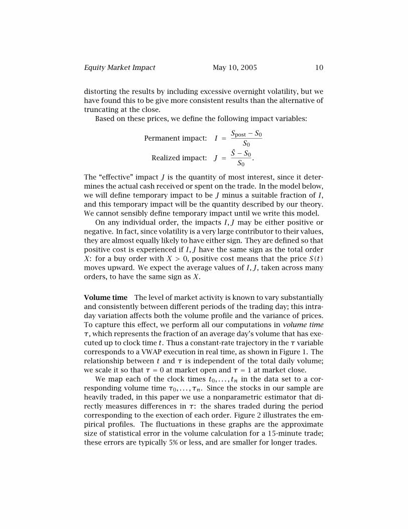
Volume time The level of market activity is known to vary substantiallyand consistently between different periods of the trading day; this intra-day variation affects both the volume profile and the variance of prices.To capture this effect, we perform all our computations in volume timeτ , which represents the fraction of an average day’s volume that has exe-cuted up to clock time t. Thus a constant-rate trajectory in the τ variablecorresponds to a VWAP execution in real time, as shown in Figure 1. Therelationship between t and τ is independent of the total daily volume;we scale it so that τ = 0 at market open and τ = 1 at market close.

We map each of the clock times t0, . . . , tn in the data set to a cor-responding volume time τ0, . . . , τn. Since the stocks in our sample areheavily traded, in this paper we use a nonparametric estimator that di-rectly measures differences in τ : the shares traded during the periodcorresponding to the exection of each order. Figure 2 illustrates the em-pirical profiles. The fluctuations in these graphs are the approximatesize of statistical error in the volume calculation for a 15-minute trade;these errors are typically 5% or less, and are smaller for longer trades.


To model more thinly traded stocks, or to implement the results ofa scheduling algorithm, one can make an analytical approximation. Forexample, one can choose a specific cubic function for the intraday profile,and estimate the shape of this function using a large variety of data.

Explanatory variables We want to describe the impacts I and J in termsof the input quantities

X =n∑j=1

xj = Total executed size in shares

T = τn − τ0 = Volume duration of active trading

Tpost = τpost − τ0 = Volume duration of impact.

As noted above, X is positive for a buy order, negative for sell. We haveexplored defining T using a size-weighted average of execution times butthe results are not substantially different. We make no use of the inter-mediate execution times τ1, . . . , τn−1, and make no use of the executionsizes except in computing the order size and the mean realised price.

We shall consistently use upper case T for elapsed volume intervals;they may be interpreted as the fraction of an average day’s volume thatwould execute between the starting and ending times.

In eventual application for trajectory optimization, the size X willbe assumed given, and the execution schedule, here represented by T ,will be optimized. In general, the solution will be a complicated time-dependent trajectory which will be parameterized by a time scale T . Forthe purposes of data modeling, we ignore the trajectory optimization andtake the schedules to be determined only by the single number T .

Auxiliary variables Although our goal is to explain the dependence ofthe impact costs I, J on order size X and trade time T , other marketvariables will influence the solution. The most important of these are

V = Average daily volume in shares, and

σ = Daily volatility.

V is a ten-day moving average. For volatility, we use an intraday esti-mator that makes use of every transaction in the day. We find that it isimportant to track changes in these variables not only between differentstocks but also across time for the same stock.


3

6

9

3

6

9

Pct ofDaily Volm

Pct ofDaily Volm

1000 1100 1200 1300 1400 1500 1600

Time of day (hours)

1.0

2.0

3.0

1.0

2.0

3.0

Volatilityof Period (%)

Volatilityof Period (%)

1000 1100 1200 1300 1400 1500 1600

Time of day (hours)

Figure 2: Ten-day average intraday volume profile (upper) and volatiltyprofile (lower), on 15-minute intervals. Our approach defines to a newtime scale determined empirically by the cumulative volume profile;implicitly this takes the volatility profile to be the same which is ap-proximately valid. Our estimation introduces statistical error which areroughly the same size as the fluctuations in these graphs.


These values serve primarily to “normalize” the active variable acrossstocks with widely varying properties. It seems natural that order sizeX should be measured as a fraction of average daily volume V : X/V is amore natural variable than X itself.

In our model presented below, order size as a fraction of average vol-ume traded during the time of execution will also be seen to be important.We estimate VT directly by taking the average volume that executed be-tween clock times t0 and tn over the previous 10 days. In fact, since inour model trade duration T appears only in the combination VT , thisavoids the need to measure T directly.

We use volatility to scale the impacts: a certain level of participationin the daily volume should cause a certain level of participation in the“normal” motion of the stock. Our empirical results show that volatilityis the most important scale factor for cost impact.

3 Trajectory Cost Model

The model we use is based on the framework developed by Almgren andChriss (2000) and Almgren (2003), with simplifications made to facilitatethe data fitting. The main simplification is the assumption that the rateof trading is constant (in volume time). In addition, we neglect cross-impact, since our data set has no information about the effect of tradingone stock on the price of another.

We decompose the price impact into two components:

• A permanent component that reflects the information transmit-ted to the market by the buy/sell imbalance. This component isbelieved to be roughly independent of trade scheduling; “stealth”trading is not admitted by this construction. In our data fit, thiscomponent will be independent of the execution time T .

• A temporary component reflects the price concession needed toattract counterparties within a specified short time interval. Thiscomponent is highly sensitive to trade scheduling; here, it will de-pend strongly on T .

More detailed conceptual frameworks have been developed (Bouchaud,Gefen, Potters, and Wyart 2004), but this easily-understood model hasbecome traditional in the industry and in academic literature (Madhavan2000).


The realized price impact is a combination of these two effects. Interms of the realized and permanent impact defined above and observedfrom the data, our model may be summarized as

Realized = Permanent + Temporary + Noise

with suitable coefficients and scaling depending on T . Thus the tempo-rary impact is obtained as a difference between the realized impact andthe permanent impact; it is not directly observable although we have atheoretical model for it.

We start with an initial desired order of X shares. We assume thatthis order is completed by uniform rate of trading over a volume timeinterval T . That is, the trade rate in volume units is v = X/T , and is heldconstant until the program is completed. Constant rate in these units isequivalent to VWAP execution during the time of execution. Note that vhas the same sign as X; thus v > 0 for an buy order and v < 0 for a sellorder. Market impact will move the price in the same direction as v .

3.1 Permanent and temporary impact

We now write our model in detail. In writing these expressions, we as-sume that the asset under discussion is a single stock, during a timeperiod within which the impact functions are reasonably homogeneous.Later we shall consider the question of how the impact functions varyacross time and among stocks.

Permanent impact Our model postulates that the asset price S(τ) fol-lows an arithmetic Brownian motion, with a drift term that depends onour trade rate v . That is,

dS = S0 g(v)dτ + S0σ dB,

where B(τ) is a standard Brownian motion (or Bachelier process), andg(v) is the permanent impact function; the only assumption we makeso far is that g(v) is increasing and has g(0) = 0. As noted above, τis volume time, representing the fraction average of an average day’svolume that has executed so far. We integrate this expression in time,taking v to equal X/T for 0 ≤ τ ≤ T , and get the permanent impact

I = T g(XT

)+ σ

√Tpost ξ (1)


where ξ ∼N (0,1) is a standard Gaussian variate.Note that if g(v) is a linear function, then the accumulated drift at

time τ is proportional to Xτ/T , the number of shares we have executedto time τ , and the total permanent impact I is proportional to the totalorder size X, independently of the time scale T .

Temporary impact The price actually received from our trades is

S̃(τ) = S(τ) + S0h(XT

),

where h(v) is the temporary impact function. For convenience, we havescaled it by the market price at the start of trading, since the time inter-vals involved are all less than one day.

This expression is a continuous-time approximation to a discrete pro-cess. A more accurate description would be to imagine that time is bro-ken into intervals such as, say, one hour or one half-hour. Within eachinterval, the average price we realise on our trades during that intervalwill be slightly less favorable than the average price that an unbiasedobserver would measure during that time interval. The unbiased priceis affected on previous trades that we have executed before this interval(as well as volatility), but not on their timing. The additional concessionduring this time interval is strongly dependent on the number of sharesthat we execute in this interval.

At constant liquidation rate, calculating the time average of the exe-cution price gives the temporary impact expression

J − I2= h

(XT

)+ σ

√√√√ T

12

(4− 3

TTpost

)χ − Tpost − T

2√Tpost

ξ

, (2)

where χ ∼ N(0,1) is independent of ξ. The term I/2 reflects the effecton the later execution prices of permanent impact caused by the earlierparts of the program.

The rather complicated error expression reflects the fluctuation of themiddle part of the Brownian motion on [0, T ] relative to its end point atTpost. It is used only for heteroskedasticity corrections in the regressionfits below.

Equations (1,2) give us explicit expressions for the permanent andtemporary cost components I, J in terms of the valus of the functionsg,h at known trade rates, together with estimates of the magnitude of


the error coming from volatility. The data-fitting procedure is in principlestraightforward: we compute the costs I, J from the transaction data,and regress those values against the order size and time as indicated, toextract directly the functions g(v),h(v).

3.2 Choice of functional form

We now address the question of what should be the structure of the per-manent impact function g(v) and the temporary impact function h(v).Even with our large sample, it is not possible to extract these functionspurely from the data; we must make a hypothesis about their structure.

We postulate that these functions are power laws, that is, that

g(v) = ±γ|v|α (3)

and

h(v) = ±η|v|β, (4)

where the numerical values of the (dimensionless) coefficients γ,η andthe exponents α,β are to be determined by linear and nonlinear regres-sion on the data. The sign is to be chosen so g(v) and h(v) have thesame sign as v .

The class of power law functions is extremely broad. It includes con-cave functions (exponent < 1), convex functions (exponent > 1), and lin-ear functions (exponent = 1). It is the functional form that is implicitlyassumed by fitting straight lines on a log-log plot, as is very common inphysics and has been done in this context, for example, by Lillo, Farmer,and Mantegna (2003).

We take the same coefficients for buy orders (v > 0) and sell orders(v < 0). It would be a trivial modification to introduce different coef-ficients γ± and η± for the two sides, but our exploratory data analysishas not indicated a strong need for this. Similarly, it would be possibleto use different coefficients for stocks traded on different exchanges butthis does not appear to be necessary.

We are far from neutral in the choice of the exponents. For the per-manent impact function, there is strong reason to prefer the linear modelwith α = 1. This is the only value for which the model is free from ar-bitrage (Huberman and Stanzl 2004) (nonlinear temporary impact func-tions do not introduce arbitrage). Furthermore, the linear function is theonly one for which the permanent price impact is independent of trading


time; this is a substantial conceptual simplification though of course itmust be supported by the data.

For temporary impact, there is ample empirical evidence indicatingthat the function should be concave, that is, 0 < β < 1. This evidencedates back to Loeb (1983) and is strongly demonstrated by the fits inLillo, Farmer, and Mantegna (2003). In particular, theoretical arguments(Barra 1997) suggest that the particular value β = 1

2 is especially plausi-ble, giving a square-root impact function.

Our approach is therefore as follows: We shall make unprejudicedfits of the power law functions to the entire data set, and determine ourbest estimates for the exponents α,β. We will then test the validity ofthe values α = 1 and beta = 1/2, to validate the linear and square rootcandidate functional forms.

Once the exponents have been selected, simple linear regression isadequate to determine the coefficients. In this regression, we use het-eroskedastic weighting with the error magnitudes from (1,2). The resultof this regression is not only values for the coefficients, but also a collec-tion of error residuals ξ and χ, which must be evaluated for normalityas the theory supposes.

Single stock fits Our data is just barely adequate to determine coeffi-cients for single stocks, for a few of the names that have largest represen-tation in our sample, and fixing the values for the exponents. We do notshow these results since they do not have enough statistical significanceto be useful. But they are a good starting point for the problem of realinterest, which is the proper way to scale the model across a universe ofstocks of widely varying properties.

4 Cross-Sectional Description

In the preceding discussion, we assumed a single asset, for which we as-sumed that changes in impact functions from one day to the next wereadequately handled by scaling the impact functions by daily volume andvolatility. But as noted above, single-stock fits are of only marginal sig-nificance for practical use.


4.1 Parameter scaling

Above we have assumed an “ideal” asset, all of whose properties are con-stant in time. For any real asset, the parameters that determine marketimpact will vary with time. For example, one would expect that executionof a given number of shares would incur higher impact costs on a daywith unusually low volume or with unusually high volatility.

We therefore assume that the natural variable for characterising thesize of an overall order or of a rate of trading is not shares per se butthe number of shares relative to a best estimate of the background flowfor that stock in the time period when trading will occur. That is, theimpact cost functions should be expressed in terms of the dimensionlessquantity X/VT rather than X itself, where V is the average number ofshares per day defined in Section 2.2.

Furthermore, we suppose the motion of the price should not be givenas a raw percentage figure, but should be expressed as a fraction of the“normal” daily motion of the price, as expressed by the volatility σ .

With both of these assumptions, we modify the expressions (1,2) to

I = σ T g(XVT

)+⟨noise

⟩(5)

J − I2= σ h

(XVT

)+⟨noise

⟩. (6)

where the “noise” is the error expressions depending on volatility. Nowg(·) and h(·) are dimensionless functions of a dimensionless variable;they are assumed to be constant in time for a single stock across dayswhen σ and V vary. We now investigate the dependence of these func-tions on cross-stock variables.

4.2 Model determination

In order to bring the full size of our data set into play, we must addressthe more complicated and less precise question of how the impact func-tions vary across stocks; that is, how they might depend on variablessuch as total market capitalization, shares outstanding, bid-ask spreador other quantities. We consider permanent and temporary impact sep-arately.

Permanent We insert a “liquidity factor” L into the permanent costfunction g(v), where L depends on the market parameters character-


izing each individual stock (in addition to daily volume and volatility).There are several candidates for the inputs to L:

• Shares outstanding: We constrain the form of L to be

L =(ΘV

)δ.

where Θ is the total number of shares outstanding, and the expo-nent δ is to be determined. The dimensionless ratio Θ/V is theinverse of “turnover,” the fraction of the company’s value tradedeach day. This is a natural explanatory variable, and has been usedin empirical studies such as Breen, Hodrick, and Korajczyk (2002).

• Bid-ask spread: We have found no consistent dependence on thebid ask spread across our sample, so we do not include it in L.

• Market capitalization: Market cap differs from shares outstandingby the price per share, so including this factor is equivalent to in-cluding a “price effect.” Our empirical studies suggest that there is apersistent price effect, as also found by Lillo, Farmer, and Mantegna(2003), but that the dependence is weak enough that we neglect itin favor of the conceptually simpler quantity Θ/V .

Temporary In extensive preliminary exploration, we have found thatthe temporary cost function h(v) does not require any stock-specificmodification: liquidity cost as a fraction of volatility depends only onshares traded as a fraction of average daily volume.

Determination of exponent After assuming the functional form ex-plained above, we confirm the model and determine the exponent δ byperforming a nonlinear regression of the form

Iσ= γ T sgn(X)

∣∣∣∣ XVT∣∣∣∣α (ΘV

)δ+ 〈noise〉 (7)

1σ

(J − I

2

)= η sgn(X)

∣∣∣∣ XVT∣∣∣∣β + 〈noise〉 (8)

where “noise” is again the heteroskedastic error term from (1), and sgnis the sign function. We use a modified Gauss-Newton optimization algo-


rithm to determine the values of γ, α, and δ that minimize the normal-ized residuals. The results are

α = 0.891 ± 0.10

δ = 0.267 ± 0.22

β = 0.600 ± 0.038.

Here, as throughout this paper, the error bars expressed with ± are onestandard deviation, assuming a Gaussian error model. Thus the “true”value can be expected to be within this range with 67% probability, andwithin a range twice as large with 95% probability.

From these values we draw the following conclusions:

• The value α = 1, for linear permanent impact, cannot reliably berejected. In view of the enormous practical simplification of linearpermanent impact, we choose to use α = 1.

• The liquidity factor is very approximately δ = 1/4.

• For temporary impact, our analysis confirms the concavity of thefunction with β strictly inferior to 1. This confirms the fact thatthe bigger the trades made by fund managers on the market, theless additional cost they experience per share traded. At the 95%confidence level, the square-root model β = 1/2 is rejected. We willtherefore fix on the temporary cost exponent β = 3/5. In compari-son with the square-root model, this gives slightly smaller costs forsmall trades, and slightly larger costs for large trades.

Note that because δ > 0, for fixed values of the number X of shares in theorder and the average daily volume V , the cost increases with Θ, the totalnumber of shares outstanding. In effect, a larger number of outstandingshares means that a smaller fraction of the company is traded each day,so a given fraction of that flow has greater impact.

Therefore these results confirm empirically the theoretical argumentsof Huberman and Stanzl (2004) for permanent impact that is linear inblock size, and the concavity of temporary impact as has been widelydescribed in the literature for both theoretical and empirical reasons.

4.3 Determination of coefficients

After fixing the exponent values, we determine the values of γ and ηby linear regression of the models (7,8), using the heteroskedastic error


estimates given in (1,2). We find

γ = 0.314 ± 0.041 (t = 7.7)η = 0.142 ± 0.0062 (t = 23).

The t statistic given here is computed under the assumption that theGaussian model expressed in (1,2) is valid; the error estimates are thevalue divided by the t statistic. Although the actual residuals are fat-tailed as we discuss below, these estimates indicate that the coefficientvalues are highly significant.

TheR2 values for these regressions are typically less than one percent,indicating that only a small part of the value of the dependent variablesI and J is explained by the model in terms of the independent variables.This is precisely what is expected, given the small size of the permanentimpact term relative to the random motion of the price due to volatilityduring the trade execution.

This persistent cost, though small, is of major importance since it is inaverage the cost incurred while trading by fund managers. Furthermore,since most orders are part of large portfolio trades, the volatility costactually experienced on the portfolio level is considerably lower thanexhibited in the stock-level analysis, increasing the significance of thefraction of impact cost estimated. As previously mentioned, the non-linear optimization of the volatility versus impact cost trade-off at theportfolio level is a subject of current work.

The dimensionless numbers γ and η are the “universal coefficients ofmarket impact:” according to our model they apply to every order andevery asset in the entire data set. To summarize, they are to be insertedinto the equations

I = γ σXV

(ΘV

)1/4+ 〈noise〉

J = I2+ sgn(X) ησ

∣∣∣∣ XVT∣∣∣∣3/5 + 〈noise〉

giving the expectation of impact costs; in any particular order the realizedvalues will vary greatly due to volatility. Recall that I is not a cost, butis simply the net price motion from pre-trade to post-trade. The actualcost experienced on the order is J.

We have chosen these simple forms in order to have a single modelthat applies reasonably well across the entire data set, which consistsentirely of large-cap stocks in the US markets. More detailed models


IBM DRIAverage daily volume V 6.561 M 1.929 MShares outstanding Θ 1728 M 168 MInverse turnover Θ/V 263 87Daily volatility (%) σ 1.57 2.26Normalized trade size X/V 0.1 0.1Normalized permanent I/σ 0.126 0.096Permanent price impact (bp) I 20 22Trade duration (days) T 0.1 0.2 0.5 0.1 0.2 0.5Normalized temporary K/σ 0.142 0.094 0.054 0.142 0.094 0.054Temporary impact cost (bp) K 22 15 8 32 21 12Realized cost (bp) J 32 25 18 43 32 23

Table 3: Example of permanent and temporary impact costs, for a pur-chase of 10% of day’s average volume, in two different large-cap stocks.The permanent cost is independent of time of execution. The tempo-rary cost depends on the time, but across different assets it is the samefraction of daily volatility. We write K = J − I/2.

could be constructed to capture more limited sets of dates or assets, or toaccount for variations across global markets. In practice, we expect thatthe coefficients, perhaps the exponents, and maybe even the functionalforms, will be continually updated to reflect the most recent data.

Examples In Figure 3 we show the impact cost functions, and in Table 3we show specific numerical examples for two large-cap stocks, when thecustomer buys 10% of the average daily volume. Because DRI turns over1/87 of its total float each day, whereas IBM turns over only 1/263, trad-ing one-tenth of one day’s volume causes a permanent price move of only0.1 times volatility for DRI, but 0.13 times for IBM; half of this is expe-rienced as cost. Because the permanent impact function is linear, thepermanent cost numbers are independent of the time scale of execution.

4.4 Residual analysis

The result of our analysis is not simply the values of the coefficientspresented above. In addition, our error formulation provides specificpredictions for the nature of the residuals ξ and χ for the permanent


0 0.05 0.1 0.15 0.20

0.05

0.1

0.15

0.2 0.001

0.01

0.1

IBM

DRI

Permanent

Normalized order size X/V

Nor

mal

ized

impa

ct I/

σ

0 0.2 0.4 0.6 0.8 10

0.05

0.1

0.15Temporary

Normalized trade rate X/VT

Nor

mal

ized

impa

ct I/

σ

Figure 3: Upper panel shows permanent price impact, giving normalizedprice motion in terms of normalized order size for three values of dailyturnover V/Θ = 0.001,0.01,0.1. Lower panel is temporary impact costfunction, in terms of normalized order rate. The examples from Table 3are also shown. For permanent cost the location on the graph dependson asset properties but not on time of trade execution; for temporarycost the location depends on time but not on asset.


and temporary impact as in Eqs. (1,2). Under the assumption that theasset price process is a Brownian motion with drift caused by our impact,these two variables should be independent standard Gaussians. We havealready used this assumption in the heteroskedastic regression, and nowwe want to verify it.

Figure 4 shows histograms and Q-Q plots of ξ and χ. The means arequite close to zero. The variances are reasonably close to 1, and the cor-relation is reasonably small. But the distribution is extremely fat-tailed,as is normal for returns distributions on short time intervals (Rydberg(2000) has a nice illustration), and hence does not indicate that the modelis poorly specified. Nonetheless, the structure of these residuals con-firms that our model is close to the best that can be done within theBrownian motion framework.

5 Summary

We have used a large data sample of US institutional orders, and a sim-ple but realistic theoretical model, to estimate price impact functions forequity trades on large-cap stocks. Within the range of order sizes con-sidered (up to about 10% of daily volume), this model can be used to givequantitatively accurate pre-trade cost estimates, and is in a form that canbe directly incorporated into optimal scheduling algorithms. Work is un-derway to refine the calibration to handle global markets, and the modelis currently being incorporated into Citigroup’s Best Execution Consult-ing Services software.

References

Alba, J. N. (2002). Transaction costs analysis: How to achieve best execution.In Best Execution: Executing Transactions in Securities Markets on behalfof Investors, pp. 6–17. European Asset Management Association. 5

Almgren, R. and N. Chriss (2000). Optimal execution of portfolio transac-tions. J. Risk 3(2), 5–39. 5, 13

Almgren, R. F. (2003). Optimal execution with nonlinear impact functionsand trading-enhanced risk. Appl. Math. Fin. 10, 1–18. 5, 13

Barra (1997). Market Impact Model Handbook. Barra. 17

Bouchaud, J.-P., Y. Gefen, M. Potters, and M. Wyart (2004). Fluctuationsand response in financial markets: The subtle nature of ‘random’ pricechanges. Quant. Finance 4(2), 176–190. 4, 13


−6 −4 −2 0 2 4 610

1

102

103

104

95%

ξ

−3 −2 −1 0 1 2 3−3

−2

−1

0

1

2

3ξ

−6 −4 −2 0 2 4 610

1

102

103

104

95%

χ

−3 −2 −1 0 1 2 3−3

−2

−1

0

1

2

3χ

Figure 4: Q-Q plots and logarithmic histograms of error residuals ξ andχ, for permanent and temporary impact respectively, from the entire 19-month sample (29,509 points). In the left column, the vertical axis is thenumber of sample values in the bin, on a log scale; the dashed line showsthe value that would be expected in a standard Gaussian distribution ofzero mean and unit variance (not adjusted to sample mean and variance).In the right column, the horizontal axis is the residual, and the verticalaxis is values of the cumulative normal; if the distribution were normalall points would lie on the dashed line. The distribution is clearly fattailed, but the standard Gaussian is a reasonable fit to the central part.


Breen, W. J., L. S. Hodrick, and R. A. Korajczyk (2002). Predicting equity liq-uidity. Management Science 48(4), 470–483. 4, 19

Chan, L. K. C. and J. Lakonishok (1995). The behavior of stock prices aroundinstitutional trades. J. Finance 50, 1147–1174. 5

de Ternay, A. (2002). Orders execution—emergence of a new added value:concerns, from regulator to operator. In Best Execution: Executing Trans-actions in Securities Markets on behalf of Investors, pp. 31–43. EuropeanAsset Management Association. 5

Dufour, A. and R. F. Engle (2000). Time and the price impact of a trade. J.Finance 55(6), 2467–2498. 4

Freyre-Sanders, A., R. Guobuzaite, and K. Byrne (Fall 2004). A review of trad-ing cost models: Reducing trading costs. J. Investing 13, 93–115. 3

Holthausen, R. W., R. W. Leftwich, and D. Mayers (1990). Large-block transac-tions, the speed of response, and temporary and permanent stock-priceeffects. J. Financial Econ. 26, 71–95. 5

Huberman, G. and W. Stanzl (2004). Price manipulation and quasi-arbitrage.Econometrica 72(4), 1247–1275. 16, 20

Keim, D. B. and A. Madhavan (1996). The upstairs market for large-blocktransactions: Analysis and measurement of price effects. Rev. FinancialStudies 9, 1–36. 5

Kissell, R. and M. Glantz (2003). Optimal Trading Strategies. Amacom. 4

Lillo, F., J. D. Farmer, and R. N. Mantegna (2003). Master curve for price-impact function. Nature 421, 129–130. 4, 16, 17, 19

Loeb, T. F. (1983). Trading cost: The critical link between investment infor-mation and results. Financial Analysts Journal 39(3), 39–44. 17

Madhavan, A. (2000). Market microstructure: A survey. J. Financial Markets 3,205–258. 13

Rydberg, T. H. (2000). Realistic statistical modelling of financial data. Inter-nat. Stat. Rev. 68(3), 233–258. 24

Rydberg, T. H. and N. Shephard (2003). Dynamics of trade-by-trade pricemovements: Decomposition and models. J. Financial Econ. 1(1), 2–25. 4

Sorensen, E. H., L. J. Price, K. L. Miller, D. E. Cox, and S. A. Birnbaum (1998).The Salomon Smith Barney global equity impact cost model. Technicalreport, Salomon Smith Barney. 4

Weisberger, D. and S. B. Kreichman (1999). The accurate measurement ofequity trading costs. Technical report, Salomon Smith Barney PortfolioTrading Strategies. 5

Direct Estimation of Equity Market Impact

Documents

Transcript of Direct Estimation of Equity Market Impact