Diptiman Sen Indian Institute of Science, Bangalore E...

The Kitaev modelDiptiman Sen

Indian Institute of Science, Bangalore

E-mail: [email protected]

Theoretical Physics Colloquium, TIFR

18th August, 2009

The Kitaev model – p.1/34

OutlineKitaev model and motivations for studying it

Mapping spin-1/2’s to Majorana fermionsConserved quantities and different sectorsComplete solution in the ground state sectorCorrelation functionsEffects of quenchingLarge-S model and spin wave theoryOutlook


OutlineKitaev model and motivations for studying itMapping spin-1/2’s to Majorana fermions

Conserved quantities and different sectorsComplete solution in the ground state sectorCorrelation functionsEffects of quenchingLarge-S model and spin wave theoryOutlook


OutlineKitaev model and motivations for studying itMapping spin-1/2’s to Majorana fermionsConserved quantities and different sectors

Complete solution in the ground state sectorCorrelation functionsEffects of quenchingLarge-S model and spin wave theoryOutlook


OutlineKitaev model and motivations for studying itMapping spin-1/2’s to Majorana fermionsConserved quantities and different sectorsComplete solution in the ground state sector

Correlation functionsEffects of quenchingLarge-S model and spin wave theoryOutlook


OutlineKitaev model and motivations for studying itMapping spin-1/2’s to Majorana fermionsConserved quantities and different sectorsComplete solution in the ground state sectorCorrelation functions

Effects of quenchingLarge-S model and spin wave theoryOutlook


OutlineKitaev model and motivations for studying itMapping spin-1/2’s to Majorana fermionsConserved quantities and different sectorsComplete solution in the ground state sectorCorrelation functionsEffects of quenching

Large-S model and spin wave theoryOutlook


OutlineKitaev model and motivations for studying itMapping spin-1/2’s to Majorana fermionsConserved quantities and different sectorsComplete solution in the ground state sectorCorrelation functionsEffects of quenchingLarge-S model and spin wave theory

Outlook


OutlineKitaev model and motivations for studying itMapping spin-1/2’s to Majorana fermionsConserved quantities and different sectorsComplete solution in the ground state sectorCorrelation functionsEffects of quenchingLarge-S model and spin wave theoryOutlook


Kitaev model

Kitaev, Ann. Phys. 321 (2006) 2

Some observations:

• A two-dimensional quantum spin model which is completely solvable

• Reduces to a problem of non-interacting Majorana fermions

• Excitations have Abelian or non-Abelian statistics

• Model has topological order


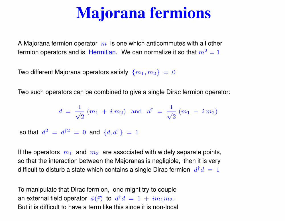
Majorana fermionsA Majorana fermion operator m is one which anticommutes with all otherfermion operators and is Hermitian. We can normalize it so that m2 = 1

Two different Majorana operators satisfy {m1, m2} = 0

Two such operators can be combined to give a single Dirac fermion operator:

d =1√2

(m1 + i m2) and d† =1√2

(m1 − i m2)

so that d2 = d†2 = 0 and {d, d†} = 1

If the operators m1 and m2 are associated with widely separate points,so that the interaction between the Majoranas is negligible, then it is verydifficult to disturb a state which contains a single Dirac fermion d†d = 1

To manipulate that Dirac fermion, one might try to couplean external field operator φ(~r) to d†d = 1 + im1m2.

But it is difficult to have a term like this since it is non-localThe Kitaev model – p.4/34

Majorana fermions · · ·

Majorana fermions separated by large distances from each other providea robust way of storing information

They may occur in certain situations such as in a fractional quantum Hallsystem with filling fraction equal to 5/2, at the core of half-vortices inlayered p−wave superconductors (such as Sr2RuO4), at theinterface of a ferromagnetic insulator and a superconductor onthe surface of a topological insulator, and perhaps in p−wavecondensates of spin-polarized 40K and 6Li atoms inoptical traps

Read and Green, Phys. Rev. B 61 (2000) 10267;Ivanov, Phys. Rev. Lett. 86 (2001) 268;Stern, von Oppen and Mariani, Phys. Rev. B 70 (2004) 205338;Tewari, Zhang, Das Sarma, Nayak and Lee, Phys. Rev. Lett. 100 (2008) 027001


Majorana fermions · · ·

Spin-1/2’s can be written in terms of Majorana fermions in many ways,all of which satisfy the anticommutation relations at the same site j andthe commutation relations between different sites j and k

• Can use three Majorana fermions (Shastry) to write σxj = − iby

j bzj ,

σyj = − ibz

j bxj and σz

j = − ibxj by

j , where the baj are Majorana fermions

• Can use four Majorana fermions (Kitaev) to write σxj = icjcx

j ,

σyj = icjcy

j and σzj = icjcz

j , where the cj and caj are Majorana

fermions, and the physical states are those which satisfy cjcxj cy

j czj = 1

Both these representations increase the dimension of the Hilbert space,giving some redundant states

This is the route Kitaev used to solve his model. We will follow a different routewhich involves Majorana fermions but does not introduce any redundant states

Feng, Zhang and Xiang, Phys. Rev. Lett. 98 (2007) 087204; Lee, Zhang and Xiang,Phys. Rev. Lett. 99 (2007) 196805; Chen and Nussinov, J. Phys. A 41 (2008) 075001


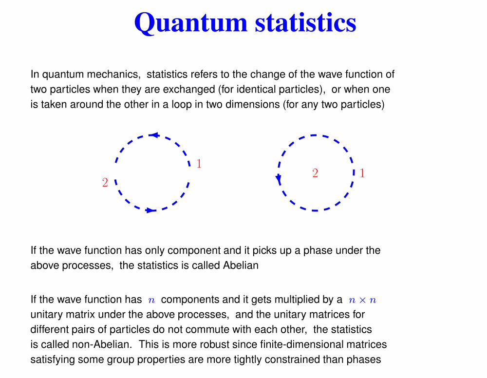
Quantum statisticsIn quantum mechanics, statistics refers to the change of the wave function oftwo particles when they are exchanged (for identical particles), or when oneis taken around the other in a loop in two dimensions (for any two particles)

1

212

If the wave function has only component and it picks up a phase under theabove processes, the statistics is called Abelian

If the wave function has n components and it gets multiplied by a n × n

unitary matrix under the above processes, and the unitary matrices fordifferent pairs of particles do not commute with each other, the statisticsis called non-Abelian. This is more robust since finite-dimensional matricessatisfying some group properties are more tightly constrained than phases


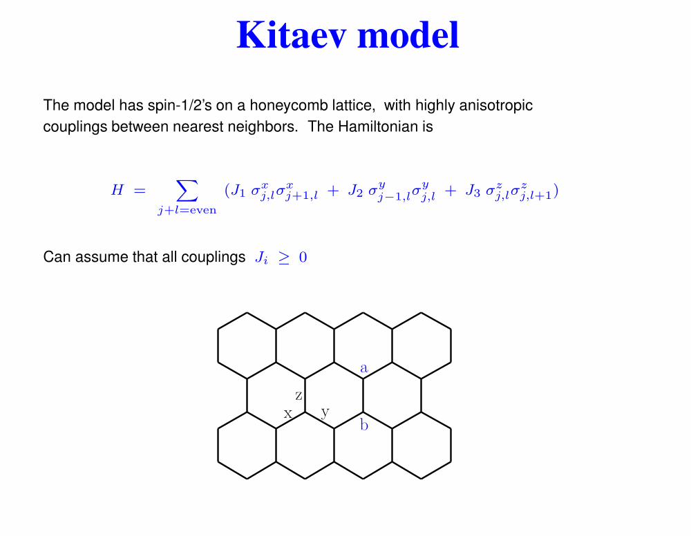
Kitaev modelThe model has spin-1/2’s on a honeycomb lattice, with highly anisotropiccouplings between nearest neighbors. The Hamiltonian is

H =X

j+l=even

(J1 σxj,lσ

xj+1,l + J2 σy

j−1,lσyj,l + J3 σz

j,lσzj,l+1)

Can assume that all couplings Ji ≥ 0

x yz

a

b


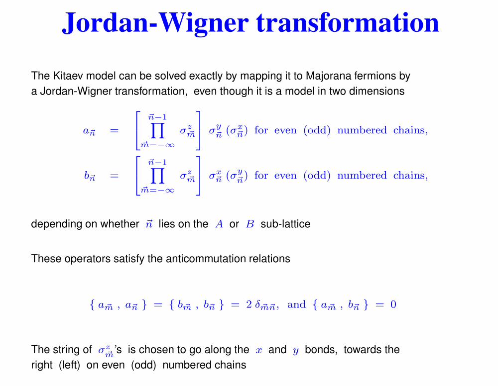
Jordan-Wigner transformationThe Kitaev model can be solved exactly by mapping it to Majorana fermions bya Jordan-Wigner transformation, even though it is a model in two dimensions

a~n =

2

4

~n−1Y

~m=−∞σz

~m

3

5 σy~n

(σx~n) for even (odd) numbered chains,

b~n =

2

4

~n−1Y

~m=−∞σz

~m

3

5 σx~n (σy

~n) for even (odd) numbered chains,

depending on whether ~n lies on the A or B sub-lattice

These operators satisfy the anticommutation relations

{ a~m , a~n } = { b~m , b~n } = 2 δ~m~n, and { a~m , b~n } = 0

The string of σz~m’s is chosen to go along the x and y bonds, towards the

right (left) on even (odd) numbered chainsThe Kitaev model – p.9/34

Jordan-Wigner transformation

H =X

j+l=even

(J1 σxj,lσ

xj+1,l + J2 σy

j−1,lσyj,l + J3 σz

j,lσzj,l+1)

The xx and yy interactions become local and quadratic in the Majoranafermions under the Jordan-Wigner transformation

The zz interaction would normally become non-local and quartic in thefermions

But in this model, this remains local and only couples fermions on nearestneighbor sites due to a large number of conserved quantities


Conserved quantities

x yz

12

3

4

56

W

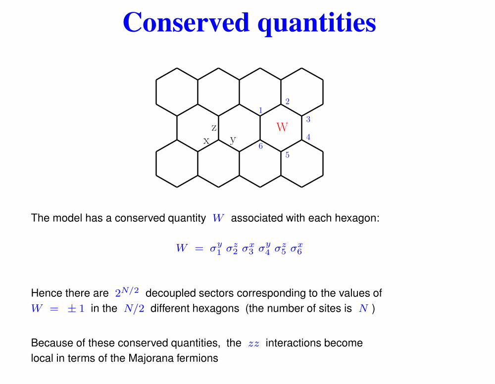
The model has a conserved quantity W associated with each hexagon:

W = σy1 σz

2 σx3 σy

4 σz5 σx

6

Hence there are 2N/2 decoupled sectors corresponding to the values ofW = ± 1 in the N/2 different hexagons (the number of sites is N )

Because of these conserved quantities, the zz interactions becomelocal in terms of the Majorana fermions


Kitaev model · · ·

1

2

W1

W2

W3

. . .

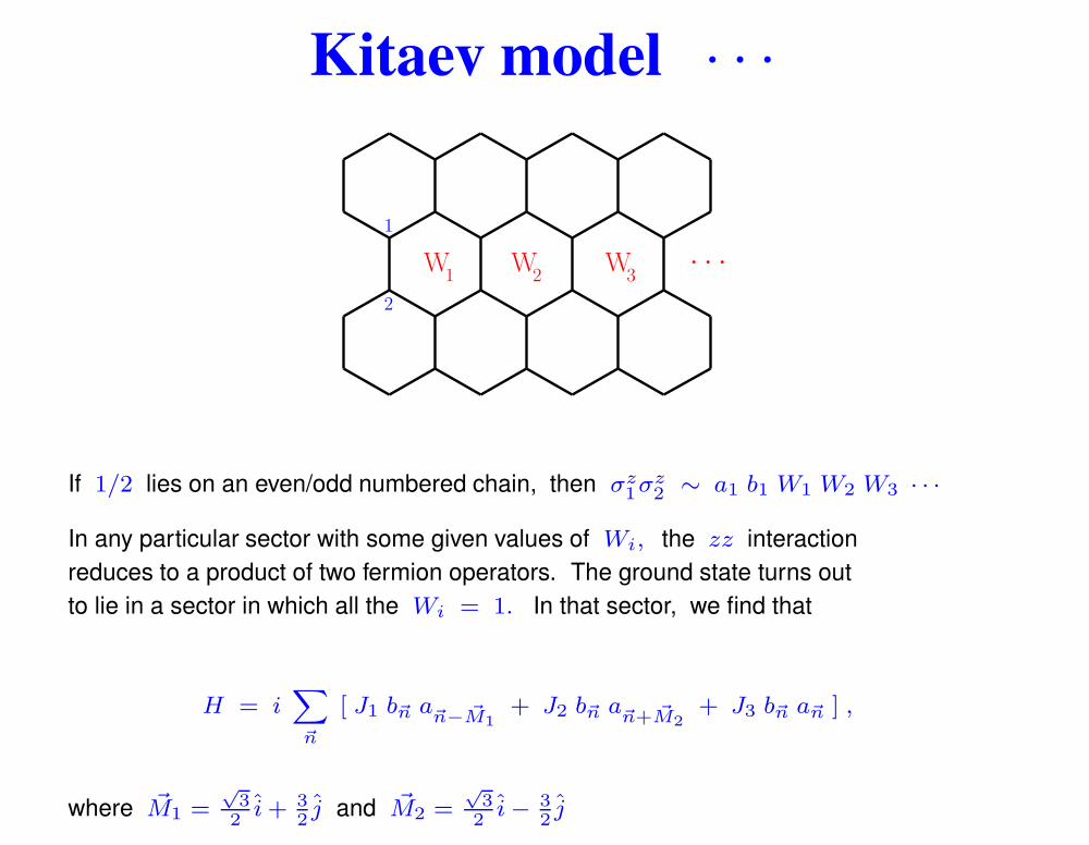
If 1/2 lies on an even/odd numbered chain, then σz1σz

2 ∼ a1 b1 W1 W2 W3 · · ·

In any particular sector with some given values of Wi, the zz interactionreduces to a product of two fermion operators. The ground state turns outto lie in a sector in which all the Wi = 1. In that sector, we find that

H = iX

~n

[ J1 b~n a~n− ~M1

+ J2 b~n a~n+ ~M2

+ J3 b~n a~n ] ,

where ~M1 =√

32

i + 32j and ~M2 =

√3

2i − 3

2j


Brillouin zoneDefine the Fourier transforms

a~n =

r

4

N

X

~k

[ a~kei~k·~n + a†

~ke−i~k·~n ],

b~n =

r

4

N

X

~k

[ b~kei~k·~n + b†

~ke−i~k·~n ],

where ~k runs over only half the Brillouin zone which looks as follows:

kx

ky

2π

3

−

2π

3

2π√

3


HamiltonianThe Hamiltonian of the Kitaev model is

H =X

~k

“

a†~k

b†~k

”

H~k

0

@

a~k

b~k

1

A ,

H~k= 2 [J3 + J1 cos(~k · ~M1) + J2 cos(~k · ~M2)] σ3

+ 2 [J1 sin(~k · ~M1) − J2 sin(~k · ~M2)] σ1,

where ~M1 =√

32

i + 32j and ~M2 =

√3

2i − 3

2j

This is a system of non-interacting Majorana fermions

Depending on the values of J1, J2, J3, there may or may not bea gap between the ground state and the first excited state


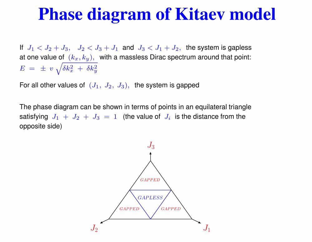
Phase diagram of Kitaev modelIf J1 < J2 + J3, J2 < J3 + J1 and J3 < J1 + J2, the system is gaplessat one value of (kx, ky), with a massless Dirac spectrum around that point:E = ± v

q

δk2x + δk2

y

For all other values of (J1, J2, J3), the system is gapped

The phase diagram can be shown in terms of points in an equilateral trianglesatisfying J1 + J2 + J3 = 1 (the value of Ji is the distance from theopposite side)

GAPLESS

GAPPEDGAPPED

GAPPED

J1J2

J3


Topological orderOn the surface of a torus, in the thermodynamic limit, the energy spectrumis independent of the product of the Wi along the two loops shown in red

The two loop variables can take the values ± 1 independently.Hence all energy levels have a degeneracy of 4

This is a signature of topological order

Recall: fractional quantum Hall states also have topological order. On a surfaceof genus g, (g = 0 and 1 for a sphere and a torus respectively), the groundstate for a quantum Hall state with filling fraction 1/3 has a degeneracy of 3g


Quantum statisticsBack to the Kitaev model on the plane: the ground state lies in the sector inwhich all the hexagonal quantities Wi = 1. This is called a vortex-free state

If Wi = −1 on any hexagon, it is called a vortex. The lowest energy statein a sector with one vortex is separated from the ground state by a finite gap;this is true in all the phases. The fermionic spectra can be gapped or gapless

In the gapped phases, the different particles (fermions and vortex) haveAbelian statistics. Taking any particle around any other, or exchangingtwo identical particles, only multiplies the wave function by ± 1

Difficult to discuss statistics for a gapless system as exchanging two particlesor taking one around the other produces low-energy excitations no matter howslowly the exchange is done, so the initial and final states are quite different

Adding a magnetic field at each site,P

i (hxσxi + hyσy

i + hzσzi ),

produces a gap, and makes it possible to discuss statistics.It also allows a vortex to move from one hexagon to anothersince the Wi do not commute with the magnetic field term


Quantum statistics · · ·

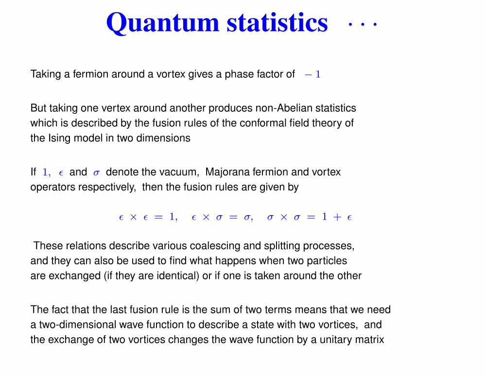
Taking a fermion around a vortex gives a phase factor of − 1

But taking one vertex around another produces non-Abelian statisticswhich is described by the fusion rules of the conformal field theory ofthe Ising model in two dimensions

If 1, ε and σ denote the vacuum, Majorana fermion and vortexoperators respectively, then the fusion rules are given by

ε × ε = 1, ε × σ = σ, σ × σ = 1 + ε

These relations describe various coalescing and splitting processes,and they can also be used to find what happens when two particlesare exchanged (if they are identical) or if one is taken around the other

The fact that the last fusion rule is the sum of two terms means that we needa two-dimensional wave function to describe a state with two vortices, andthe exchange of two vortices changes the wave function by a unitary matrix


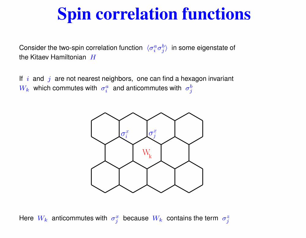
Spin correlation functionsConsider the two-spin correlation function 〈σa

i σbj〉 in some eigenstate of

the Kitaev Hamiltonian H

If i and j are not nearest neighbors, one can find a hexagon invariantWk which commutes with σa

i and anticommutes with σbj

σxi

σxj

Wk

Here Wk anticommutes with σxj because Wk contains the term σz

j


Spin correlation functions · · ·

Since we can choose every eigenstate of H to also be an eigenstateof Wk, with eigenvalue ± 1, we have〈σa

i σbj〉 = 〈Wkσa

i σbjWk〉 = 〈σa

i WkσbjWk〉 = − 〈σa

i σbj〉,

which implies that 〈σai σb

j〉 = 0

A similar argument shows that if i and j are nearest neighbors, andthe bond joining them has, say, an xx interaction, then 〈σa

i σbj〉 = 0

if either a or b is different from x

Thus, 〈σai σb

j〉 6= 0 only if i and j are nearest neighbors and a = b

is equal to the type of bond which joins i and j

Thus the two-spin correlation functions are extremely short-ranged andof a very special type

Baskaran, Mandal and Shankar, Phys. Rev. Lett. 98 (2007) 247201



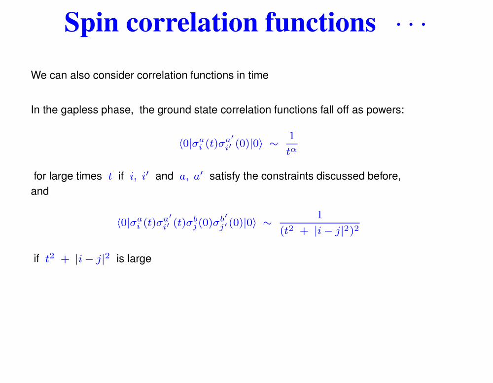
We can also consider correlation functions in time

In the gapless phase, the ground state correlation functions fall off as powers:

〈0|σai (t)σa′

i′ (0)|0〉 ∼ 1

tα

for large times t if i, i′ and a, a′ satisfy the constraints discussed before,and

〈0|σai (t)σa′

i′ (t)σbj(0)σ

b′

j′ (0)|0〉 ∼ 1

(t2 + |i − j|2)2

if t2 + |i − j|2 is large



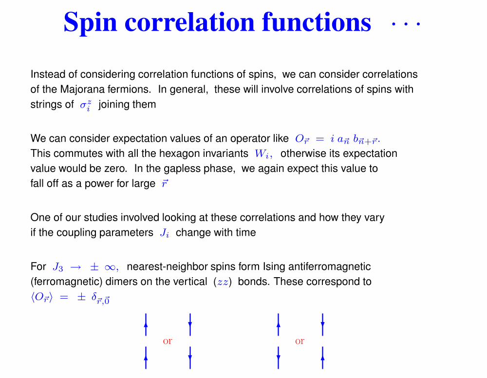
Instead of considering correlation functions of spins, we can consider correlationsof the Majorana fermions. In general, these will involve correlations of spins withstrings of σz

i joining them

We can consider expectation values of an operator like O~r = i a~n b~n+~r .

This commutes with all the hexagon invariants Wi, otherwise its expectationvalue would be zero. In the gapless phase, we again expect this value tofall off as a power for large ~r

One of our studies involved looking at these correlations and how they varyif the coupling parameters Ji change with time

For J3 → ± ∞, nearest-neighbor spins form Ising antiferromagnetic(ferromagnetic) dimers on the vertical (zz) bonds. These correspond to〈O~r〉 = ± δ~r,~0

or or


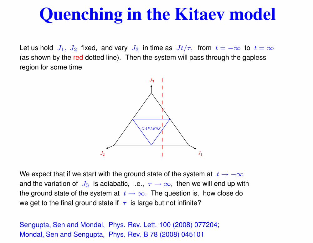
Quenching in the Kitaev modelLet us hold J1, J2 fixed, and vary J3 in time as Jt/τ, from t = −∞ to t = ∞(as shown by the red dotted line). Then the system will pass through the gaplessregion for some time

GAPLESS

J1J2

J3

We expect that if we start with the ground state of the system at t → −∞and the variation of J3 is adiabatic, i.e., τ → ∞, then we will end up withthe ground state of the system at t → ∞. The question is, how close dowe get to the final ground state if τ is large but not infinite?

Sengupta, Sen and Mondal, Phys. Rev. Lett. 100 (2008) 077204;Mondal, Sen and Sengupta, Phys. Rev. B 78 (2008) 045101 The Kitaev model – p.23/34

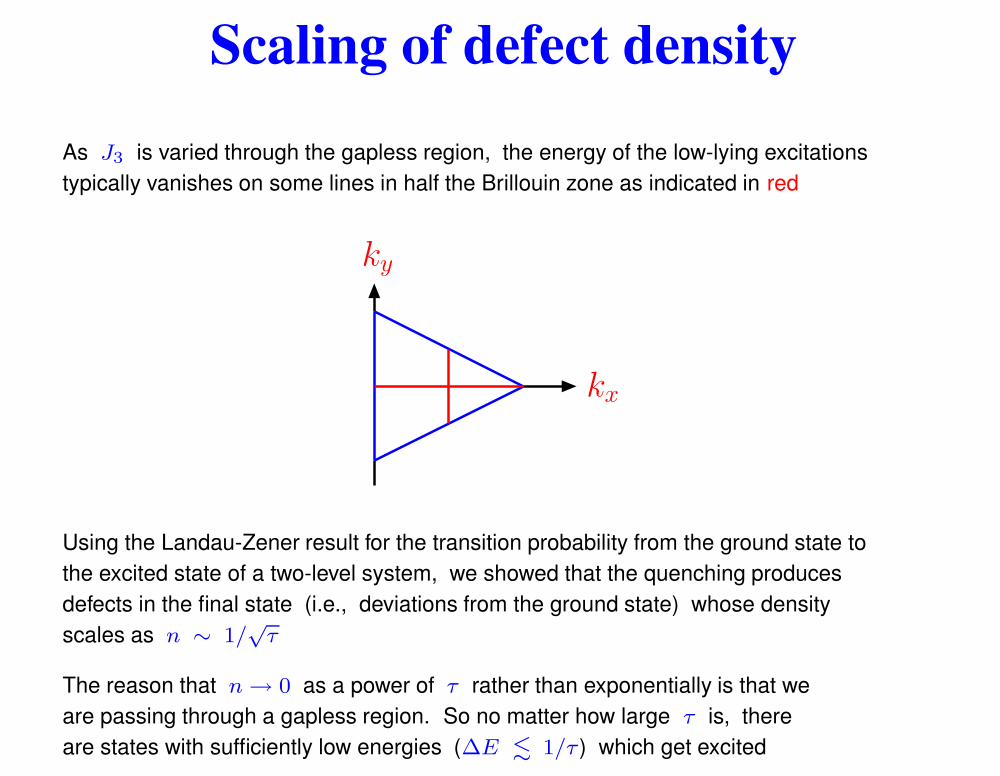
Scaling of defect densityAs J3 is varied through the gapless region, the energy of the low-lying excitationstypically vanishes on some lines in half the Brillouin zone as indicated in red

kx

ky

Using the Landau-Zener result for the transition probability from the ground state tothe excited state of a two-level system, we showed that the quenching producesdefects in the final state (i.e., deviations from the ground state) whose densityscales as n ∼ 1/

√τ

The reason that n → 0 as a power of τ rather than exponentially is that weare passing through a gapless region. So no matter how large τ is, thereare states with sufficiently low energies (∆E . 1/τ ) which get excited The Kitaev model – p.24/34

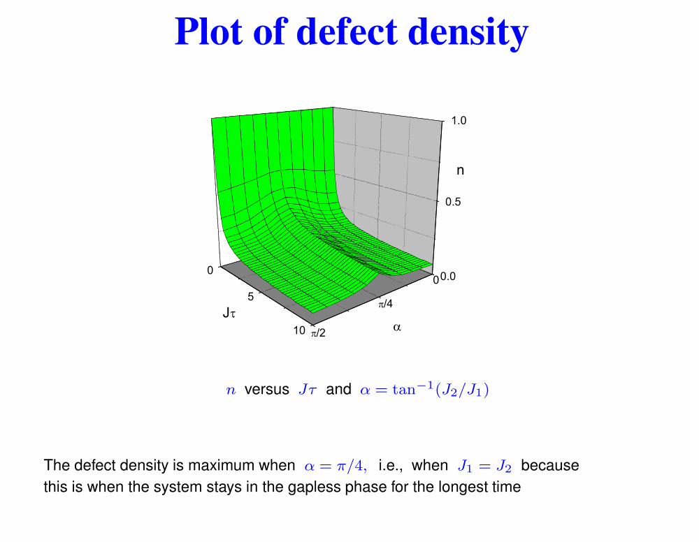
Plot of defect density

n versus Jτ and α = tan−1(J2/J1)

The defect density is maximum when α = π/4, i.e., when J1 = J2 becausethis is when the system stays in the gapless phase for the longest time


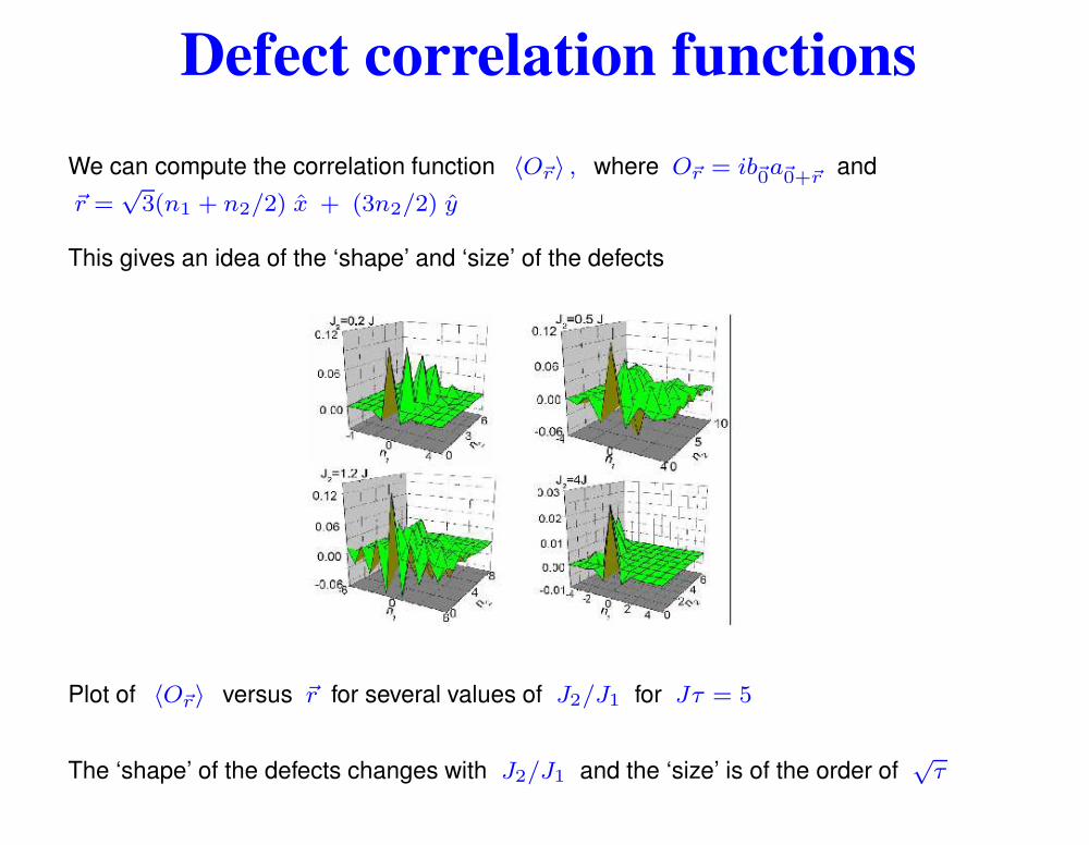
Defect correlation functionsWe can compute the correlation function 〈O~r〉 , where O~r = ib~0a~0+~r and~r =

√3(n1 + n2/2) x + (3n2/2) y

This gives an idea of the ‘shape’ and ‘size’ of the defects

Plot of 〈O~r〉 versus ~r for several values of J2/J1 for Jτ = 5

The ‘shape’ of the defects changes with J2/J1 and the ‘size’ is of the order of √τ


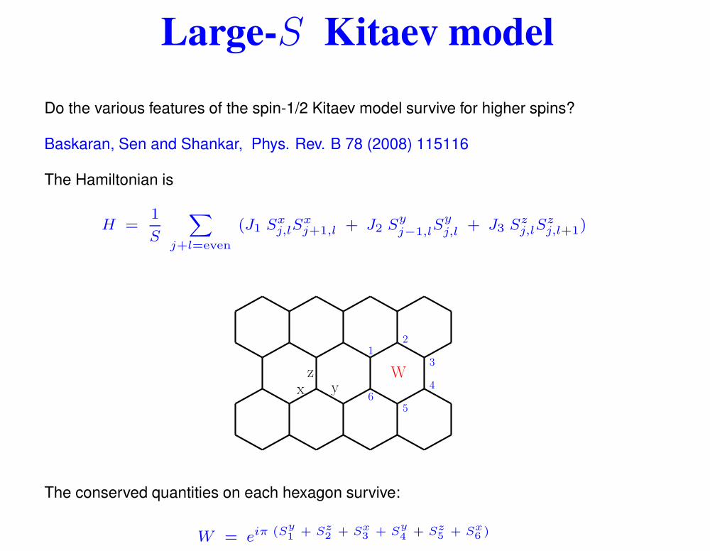
Large-S Kitaev modelDo the various features of the spin-1/2 Kitaev model survive for higher spins?

Baskaran, Sen and Shankar, Phys. Rev. B 78 (2008) 115116

The Hamiltonian is

H =1

S

X

j+l=even

(J1 Sxj,lS

xj+1,l + J2 Sy

j−1,lSyj,l + J3 Sz

j,lSzj,l+1)

x yz

12

3

4

56

W

The conserved quantities on each hexagon survive:

W = eiπ (Sy

1+ Sz

2+ Sx

3+ S

y

4+ Sz

5+ Sx

6) The Kitaev model – p.27/34

Large-S Kitaev model · · ·

H =1

S

X

j+l=even

(J1 Sxj,lS

xj+1,l + J2 Sy


j,lSzj,l+1)

The most interesting situation arises if J1 = J2 = J3

Then there are continuous families of classical ground states, for instance,all the spins on the A sublattice pointing in some direction and all the spinson the B sublattice pointing in the opposite direction

Apart from these continuous families, there is also a discrete set of groundstates in which pairs of nearest neighbor spins on, say, a xx bond pointalong the ± x direction

The number of such discrete states is equal to the number of dimer coveringsof the honeycomb lattice which is 1.175N times 1.414N (due to the choiceof ±), which gives 1.662N discrete classical ground states


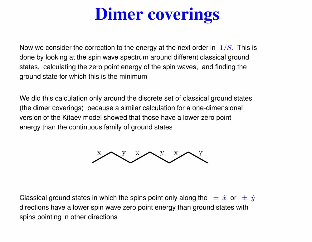
Dimer coveringsNow we consider the correction to the energy at the next order in 1/S. This isdone by looking at the spin wave spectrum around different classical groundstates, calculating the zero point energy of the spin waves, and finding theground state for which this is the minimum

We did this calculation only around the discrete set of classical ground states(the dimer coverings) because a similar calculation for a one-dimensionalversion of the Kitaev model showed that those have a lower zero pointenergy than the continuous family of ground states

x y x y x y

Classical ground states in which the spins point only along the ± x or ± y

directions have a lower spin wave zero point energy than ground states withspins pointing in other directions


Dimer coverings · · ·

For each dimer covering, there is a set of self-avoiding walks (SAWs) covering thelattice such that none of bonds appearing on the SAW is a dimer. For instance, aSAW is shown by 1’s below

1

1

1

1

1

1

1

To do a spin wave analysis, we make a Holstein-Primakoff transformation froma large spin to a harmonic oscillator. For a spin pointing in the z direction,we define Sz = S − (p2 + q2)/2, Sx =

√S q and Sy =

√S p

We then write the spin Hamiltonian up to second order in the p’s and q’sThe Kitaev model – p.30/34

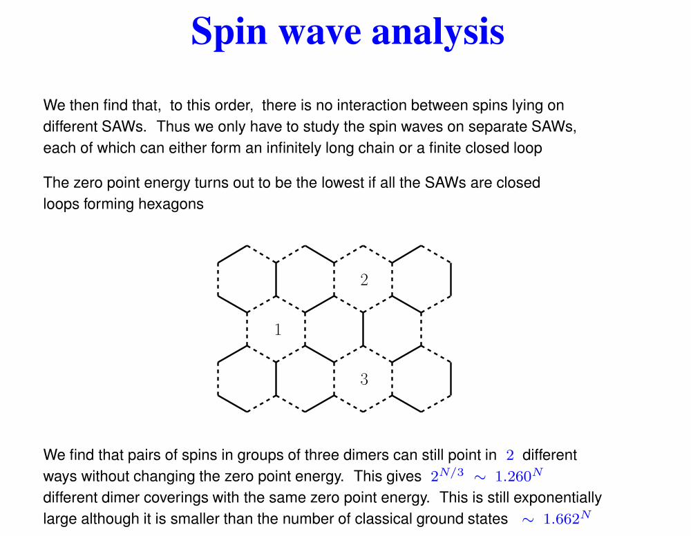
Spin wave analysisWe then find that, to this order, there is no interaction between spins lying ondifferent SAWs. Thus we only have to study the spin waves on separate SAWs,each of which can either form an infinitely long chain or a finite closed loop

The zero point energy turns out to be the lowest if all the SAWs are closedloops forming hexagons

1

2

3

We find that pairs of spins in groups of three dimers can still point in 2 differentways without changing the zero point energy. This gives 2N/3 ∼ 1.260N

different dimer coverings with the same zero point energy. This is still exponentiallylarge although it is smaller than the number of classical ground states ∼ 1.662N The Kitaev model – p.31/34

Spin wave analysis · · ·

H =1

S

X

j+l=even

(J1 Sxj,lS

xj+1,l + J2 Sy


j,lSzj,l+1)

What happens if the three couplings are not equal? If J3 is larger than theother two, the classical ground states are those in which pairs of spins oneach zz bond form antiferromagnetic dimers. The number of such states is2N/2 if the number of sites is N

The degeneracy between this discrete set of classical ground states is notbroken by the zero point energy of the spin waves


Generalizations of Kitaev modelThe Kitaev model involves three anticommuting matrices at each site, anda coordination number of three

This can be extended to a model obtained by replacing each point of thehoneycomb lattice by a triangle

Yao and Kivelson, Phys. Rev. Lett. 99 (2007) 247203

or to a lattice in three dimensions

Mandal and Surendran, Phys. Rev. B 79 (2009) 024426

The model can be generalized to have four anticommuting matrices (like the Diracmatrices) at each site, and a coordination number of four such as a square lattice

Yao, Zhang and Kivelson, Phys. Rev. Lett. 102 (2009) 217202

or more complicated lattices

Wu, Arovas and Hung, arXiv:0811.1380 The Kitaev model – p.33/34

Outlook

Effect of disorder and doping on the Kitaev model

Higher spin Kitaev models: a Jordan-Wigner transformation naturally leadsto Majorana fermion operators for half-odd-integer spins and hard coreboson operators for integer spins

The spin-1/2 Kitaev chain is completely solvable and is known to be gapless,while preliminary studies of the spin-1 model shows that it has a small gap.The integer spin chain has N conserved quantities while the half-odd-integerspin chain has N/2 conserved quantities


Diptiman Sen Indian Institute of Science, Bangalore E...

Documents

Transcript of Diptiman Sen Indian Institute of Science, Bangalore E...