1 

 

Author version: Environ. Monit. Assess., vol.182; 2011; 15–30

Dinoflagellate community structure from the stratified environment of the Bay of Bengal, with

special emphasis on Harmful Algal Bloom species

Ravidas Krishna Naik • Sahana Hegde • Arga Chandrashekar Anil

National Institute of Oceanography, Council of Scientific and Industrial Research, Dona Paula, Goa, 403004, India

ABSTRACT Harmful Algal Blooms have been documented along the coasts of India and the ill effects felt by

society at large. Most of these reports are from the Arabian Sea, west coast of India whereas its counterpart, the

Bay of Bengal (BOB) has remained unexplored in this context. The unique characteristic features of the BOB,

such as large amount of riverine fresh water discharges, monsoonal clouds, rainfall and weak surface winds make

the area strongly stratified. In this study, 19 potentially harmful species which accounted for approximately 14%

of the total identified species (134) of dinoflagellates were encountered in surface waters of the BOB during

November 2003 - September 2006. The variations in species abundance could be attributed to the seasonal

variations in the stratification observed in the BOB. The presence of frequently occurring HAB species in low

abundance (≤40 cell L-1) in stratified waters of the BOB may not be a growth issue. However, they may play a

significant role in the development of pelagic seed banks, which can serve as inocula for blooms if coupled with

local physical processes like eddies and cyclones. The predominance of Ceratium furca and Noctiluca scintillans,

frequently occurring HAB species during cyclone-prone seasons, point out their candidature for HABs.

Keywords Ceratium furca • Noctiluca scintillans • Bay of Bengal • Stratification • Cyclones • Eddies

R. K. Naik · S. Hegde · A. C. Anil ( ) Tel.: 091-832-2450404; fax: 091-832-2450615

National Institute of Oceanography,

Council of Scientific and Industrial Research,

Dona Paula, Goa, 403 004, India

E-mail: acanil@nio.org

2 

 

Introduction

Harmful Algal Blooms (HABs) are natural phenomena; historical records indicate their occurrence long before

the advent of human activities in coastal ecosystems. Recent surveys have demonstrated a dramatic increase and

geographic spread in HAB events in the last few decades (Anderson 1989; Smayda 1990; Hallegraeff 1993).

Thus, knowledge of the present geographic distribution and seasonal fluctuations in HAB species is important to

understand globally spreading HAB events (GEOHAB 2001). In fact, Hallegraeff (2010) has reported that

unpreparedness for such significant range expansions or spreading of HAB problems in poorly monitored areas

will be one of the greatest problems for human society in the future.

Among the total marine phytoplankton species, approximately 7% are capable of forming algal blooms (red

tides) (Sournia 1995); dinoflagellates are the most important group producing toxic and harmful algal blooms

(Steidinger 1983, 1993; Anderson 1989; Hallegraeff 1993) accounting for 75% of the total HAB species (Smayda

1997).

Blooms result from a coupling mechanism involving physical, chemical and biological factors. Though

dynamics of blooms is complex, the role or mechanism of chemical and biological factors are now reasonably

understood (Fistarol et al. 2004; Solé et al. 2006; GEOHAB 2006; Adolf et al. 2007; Waggett et al. 2008).

However comparable understanding about physical factors is lacking except for few examples (Maclean 1989;

Karl et al. 1997; Belgrano, 1999; Yin et al. 1999). Impacts of these factors in combination with local inter-annual

meteorological conditions will vary from one geographical location to the other and will thus influence bloom

dynamics differentially.

HAB studies in Indian waters indicate reasonable reports on HABs and their impacts along the west coast of

India. Direct impacts of HABs on human health have also been reported from Mangalore (Karunasagar et al.

1984); they related the death of a boy to an outbreak of Paralytic Shellfish Poisoning (PSP) following

consumption of clams. Dinoflagellate toxins have also been recorded in shellfish from surrounding estuaries near

Mangalore in 1985 and 1986 (Segar et al. 1989). Planktonic and cyst forms of Gymnodinium catenatum, a PSP-

producing dinoflagellate from this region were detected later on (Godhe et al. 1996) and the importance of close

monitoring of coastal waters, sediment and shellfish was highlighted.

Compared to the above regions, the Bay of Bengal (BOB), the eastern arm of the Indian Ocean, remains

relatively unexplored in the context of HAB studies. The BOB is known for its unique characteristic features:

large volume of freshwater input from river discharge and rainfall, warmer sea surface temperatures, monsoonal

clouds and reversal of currents. The riverine input into this area injects loads of nutrients and suspended sediment

3 

 

in the BOB (Gordon et al. 2002; Mukhopadhyay et al. 2006). These features point to the suitability of the BOB as

a zone prone for algal blooms including HAB events. However, the strongly stratified surface layer of the BOB

restricts the transport of nutrients from deeper layers to the surface (Prasanna Kumar et al. 2002). Thus, it is very

interesting to understand the seasonal variations in dinoflagellate community structure in this inimitable

geographic region.

Since taking oceanic cruises on regular intervals is not cost-effective, the ‘ships of opportunity’ programme,

supported by the Indian Expendable Bathythermograph (XBT) project, was used. Therefore, the present study on

the spatial and temporal distribution of dinoflagellates in the BOB, with emphasis on HAB species, is the first of

its kind from the region. The following objectives were addressed. (1) Dinoflagellate distribution in the surface

waters of the BOB and (2) Detailing of the HAB species present and their seasonal occurrence.

Materials and Methods

Study area and sampling

This study was conducted with the support of the XBT programme. Surface water samples were collected using

steel buckets from the moving ship. This method was selected in order to minimize the physical damage to cells

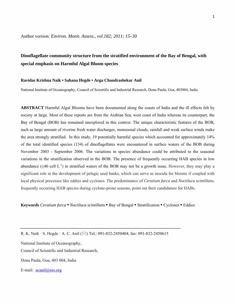
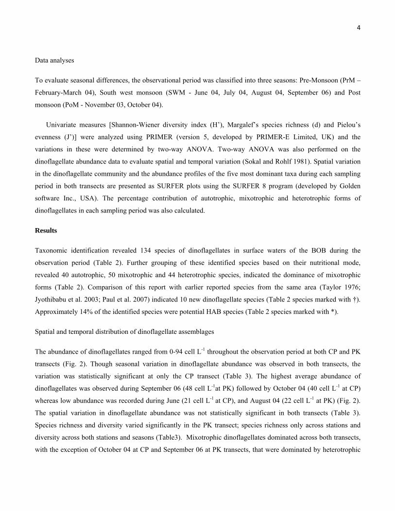
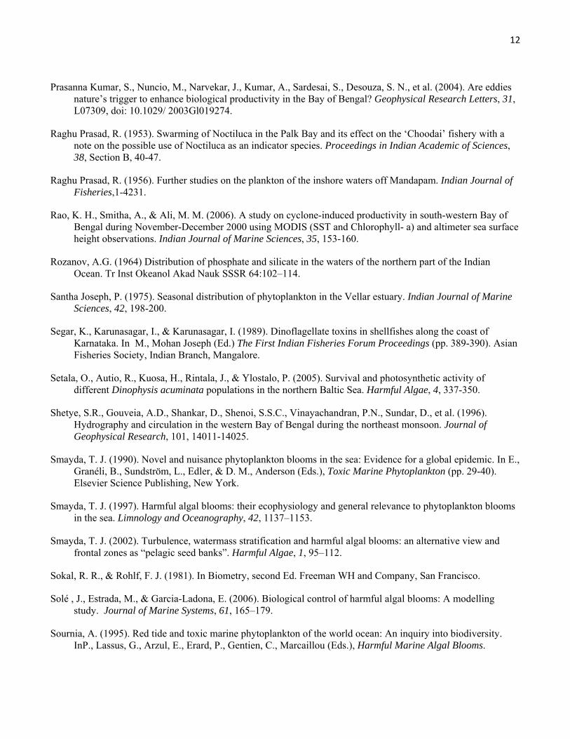
compared to the method of collecting samples using a pump. The samples were collected on 2 transects [Chennai

to Port Blair (CP, 12 stations) and Port Blair to Kolkata (PK, 10 stations)] (Fig. 1), from passenger ships plying

along these transects. Samples were collected at one degree intervals along both transect, from November 2003 to

September 2006 covering different seasons. Among the sampling stations from CP (central BOB) and PK

(northern BOB) transects, the majority were oceanic whereas, few stations are near the coast (Table 1). Samples

(1L) were fixed with Lugol’s iodine solution for the laboratory enumeration and identification of dinoflagellates

to the lowest possible taxonomic level.

Microscopic analysis

The 1L sample was kept for settling for 48 hours. After that, the volume was brought down to 100ml and then to

10 ml final concentration after another 48 hours settling period (method modified from Hasle 1978). From this 10

ml final concentration, 3 ml concentrated sample was taken in a petri dish (3.8 cm diameter) and examined under

an Olympus inverted microscope at 100X to 400X magnification. Identification of the dinoflagellate taxa was

carried out using the keys provided by Subramanyan (1968), Taylor (1976), Tomas (1997), Horner (2002) and

Hallegraeff (2003).

4 

 

Data analyses

To evaluate seasonal differences, the observational period was classified into three seasons: Pre-Monsoon (PrM –

February-March 04), South west monsoon (SWM - June 04, July 04, August 04, September 06) and Post

monsoon (PoM - November 03, October 04).

Univariate measures [Shannon-Wiener diversity index (H’), Margalef’s species richness (d) and Pielou’s

evenness (J’)] were analyzed using PRIMER (version 5, developed by PRIMER-E Limited, UK) and the

variations in these were determined by two-way ANOVA. Two-way ANOVA was also performed on the

dinoflagellate abundance data to evaluate spatial and temporal variation (Sokal and Rohlf 1981). Spatial variation

in the dinoflagellate community and the abundance profiles of the five most dominant taxa during each sampling

period in both transects are presented as SURFER plots using the SURFER 8 program (developed by Golden

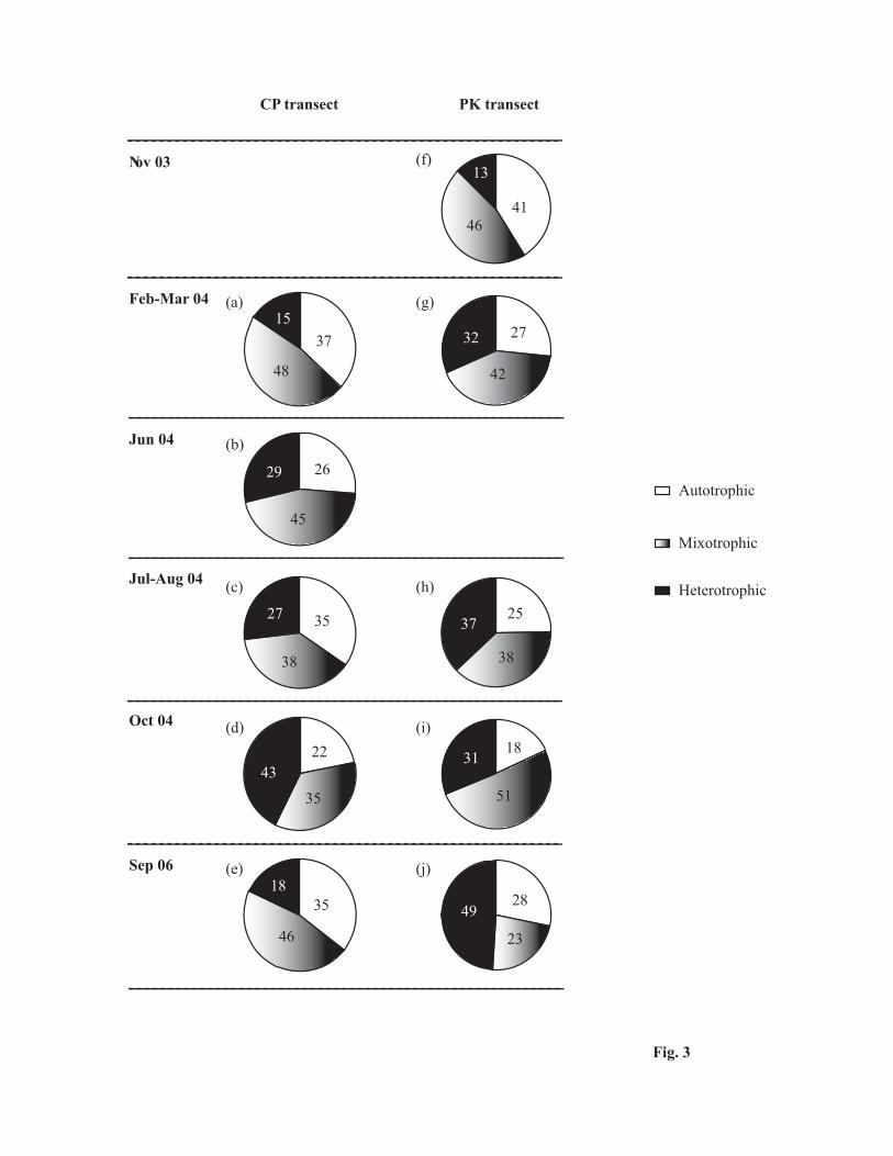
software Inc., USA). The percentage contribution of autotrophic, mixotrophic and heterotrophic forms of

dinoflagellates in each sampling period was also calculated.

Results

Taxonomic identification revealed 134 species of dinoflagellates in surface waters of the BOB during the

observation period (Table 2). Further grouping of these identified species based on their nutritional mode,

revealed 40 autotrophic, 50 mixotrophic and 44 heterotrophic species, indicated the dominance of mixotrophic

forms (Table 2). Comparison of this report with earlier reported species from the same area (Taylor 1976;

Jyothibabu et al. 2003; Paul et al. 2007) indicated 10 new dinoflagellate species (Table 2 species marked with †).

Approximately 14% of the identified species were potential HAB species (Table 2 species marked with *).

Spatial and temporal distribution of dinoflagellate assemblages

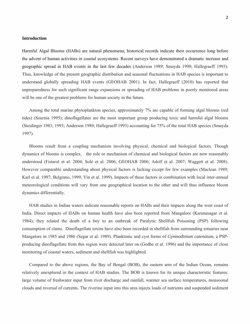
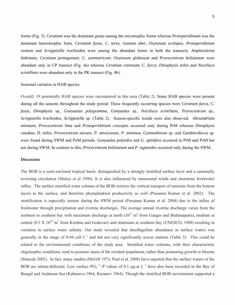
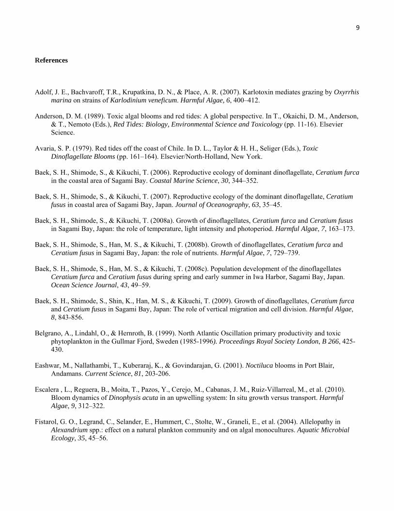
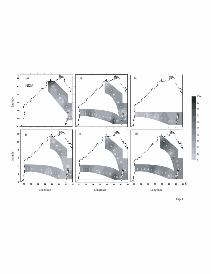
The abundance of dinoflagellates ranged from 0-94 cell L-1 throughout the observation period at both CP and PK

transects (Fig. 2). Though seasonal variation in dinoflagellate abundance was observed in both transects, the

variation was statistically significant at only the CP transect (Table 3). The highest average abundance of

dinoflagellates was observed during September 06 (48 cell L-1at PK) followed by October 04 (40 cell L-1 at CP)

whereas low abundance was recorded during June (21 cell L-1 at CP), and August 04 (22 cell L-1 at PK) (Fig. 2).

The spatial variation in dinoflagellate abundance was not statistically significant in both transects (Table 3).

Species richness and diversity varied significantly in the PK transect; species richness only across stations and

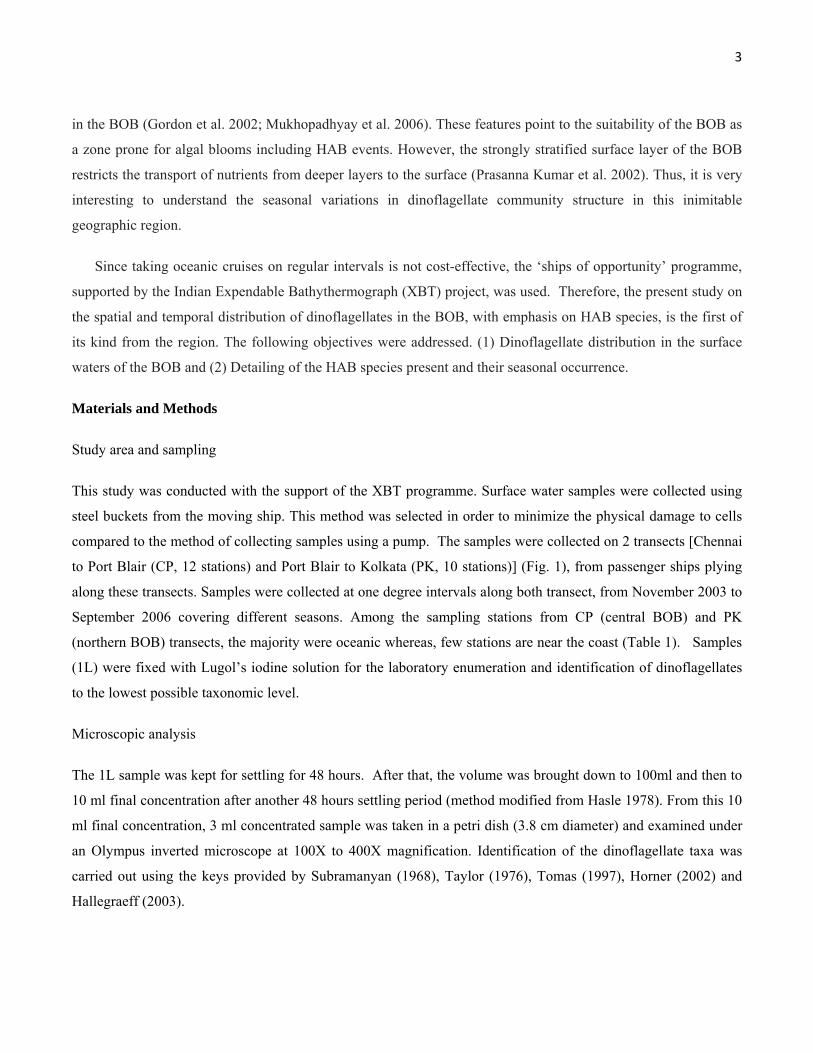
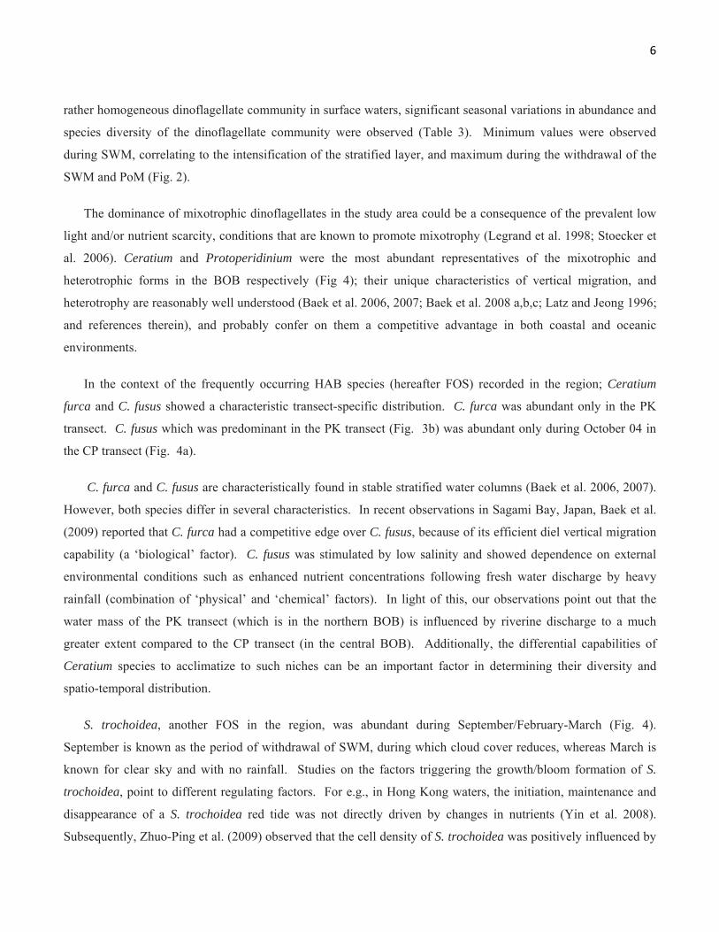
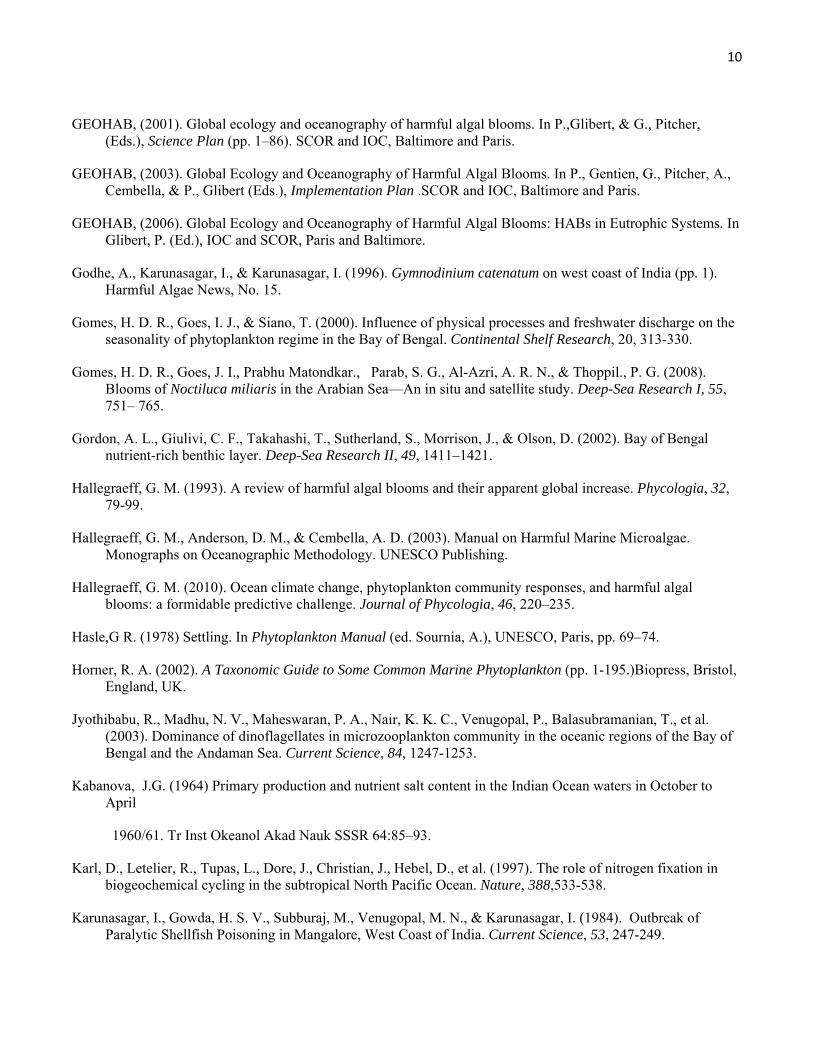
diversity across both stations and seasons (Table3). Mixotrophic dinoflagellates dominated across both transects,

with the exception of October 04 at CP and September 06 at PK transects, that were dominated by heterotrophic

5 

 

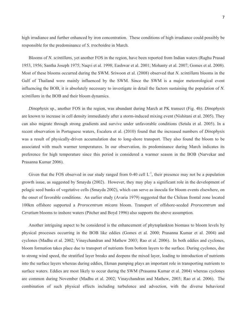
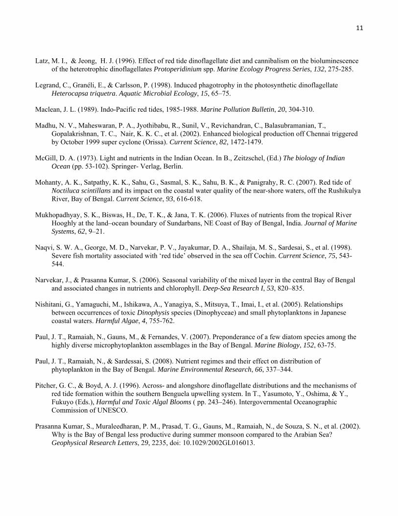
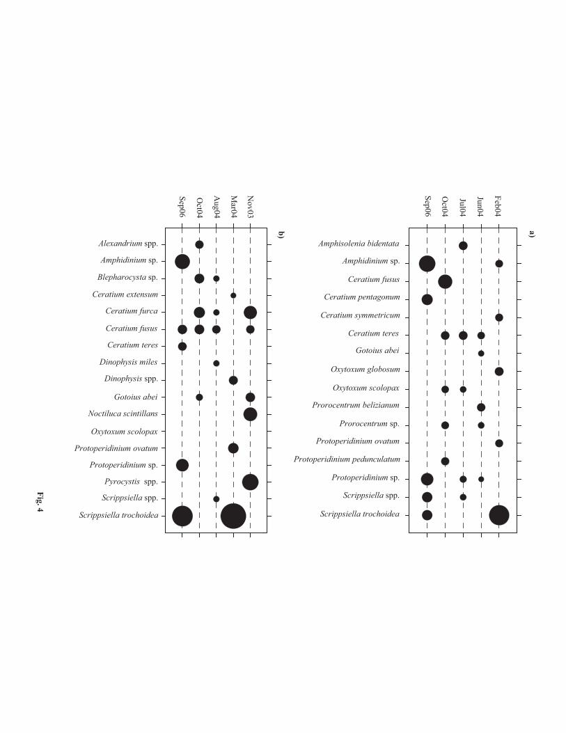
forms (Fig. 3). Ceratium was the dominant genus among the mixotrophic forms whereas Protoperidinium was the

dominant heterotrophic form. Ceratium fusus, C. teres, Gotoius abei, Oxytoxum scolopax, Protoperidinium

ovatum and Scrippsiella trochoidea were among the abundant forms in both the transects. Amphisolenia

bidentata, Ceratium pentagonum, C. symmetricum, Oxytoxum globosum and Prorocentrum belizianum were

abundant only in CP transect (Fig. 4a) whereas Ceratium extensum, C. furca, Dinophysis miles and Noctiluca

scintillans were abundant only in the PK transect (Fig. 4b).

Seasonal variation in HAB species

Overall, 19 potentially HAB species were encountered in this area (Table 2). Some HAB species were present

during all the seasons throughout the study period. These frequently occurring species were Ceratium furca, C.

fusus, Dinophysis sp., Gonyaulax polygramma, Gonyaulax sp., Noctiluca scintillans, Prorocentrum sp.,

Scrippsiella trochoidea, Scrippsiella sp. (Table 2). Season-specific trends were also observed. Alexandrium

minutum, Prorocentrum lima and Protoperidinium crassipes occurred only during PrM whereas Dinophysis

caudata, D. miles, Prorocentrum micans, P. mexicanum, P. minimus, Gymnodinium sp. and Gambierdiscus sp.

were found during SWM and PoM periods. Gonyaulax polyedra and G. spinifera occurred in PrM and PoM but

not during SWM. In contrast to this, Prorocentrum belizianum and P. sigmoides occurred only during the SWM.

Discussion

The BOB is a semi-enclosed tropical basin, distinguished by a strongly stratified surface layer and a seasonally

reversing circulation (Shetye et al 1996). It is also influenced by monsoonal winds and enormous freshwater

influx. The surface stratified water column of the BOB restricts the vertical transport of nutrients from the bottom

layers to the surface, and therefore phytoplankton productivity as well (Prasanna Kumar et al. 2002). The

stratification is especially intense during the SWM period (Prasanna Kumar et al. 2004) due to the influx of

freshwater through precipitation and riverine discharges. The average annual riverine discharge varies from the

northern to southern bay with maximum discharge at north (1012 m3 from Ganges and Brahmaputra), medium at

central (8.5 X 1010 m3 from Krishna and Godavari) and minimum at southern bay (UNESCO, 1988) resulting in

variation in surface water salinity. Our study revealed that dinoflagellate abundance in surface waters was

generally in the range of 0-94 cell L-1 and did not vary significantly across stations (Table 3). This could be

related to the environmental conditions of the study area. Stratified water columns, with their characteristic

oligotrophic conditions, tend to promote stasis of the resident population, rather than promoting growth or blooms

(Smayda 2002). In fact, many studies (McGill 1973; Paul et al. 2008) have reported that the surface waters of the

BOB are nitrate-deficient. Low surface PO4 3–-P values of 0.1 µg-at L–1 have also been recorded in the Bay of

Bengal and Andaman Sea (Kabanova 1964, Rozanov 1964). Though the stratified BOB environment supported a

6 

 

rather homogeneous dinoflagellate community in surface waters, significant seasonal variations in abundance and

species diversity of the dinoflagellate community were observed (Table 3). Minimum values were observed

during SWM, correlating to the intensification of the stratified layer, and maximum during the withdrawal of the

SWM and PoM (Fig. 2).

The dominance of mixotrophic dinoflagellates in the study area could be a consequence of the prevalent low

light and/or nutrient scarcity, conditions that are known to promote mixotrophy (Legrand et al. 1998; Stoecker et

al. 2006). Ceratium and Protoperidinium were the most abundant representatives of the mixotrophic and

heterotrophic forms in the BOB respectively (Fig 4); their unique characteristics of vertical migration, and

heterotrophy are reasonably well understood (Baek et al. 2006, 2007; Baek et al. 2008 a,b,c; Latz and Jeong 1996;

and references therein), and probably confer on them a competitive advantage in both coastal and oceanic

environments.

In the context of the frequently occurring HAB species (hereafter FOS) recorded in the region; Ceratium

furca and C. fusus showed a characteristic transect-specific distribution. C. furca was abundant only in the PK

transect. C. fusus which was predominant in the PK transect (Fig. 3b) was abundant only during October 04 in

the CP transect (Fig. 4a).

C. furca and C. fusus are characteristically found in stable stratified water columns (Baek et al. 2006, 2007).

However, both species differ in several characteristics. In recent observations in Sagami Bay, Japan, Baek et al.

(2009) reported that C. furca had a competitive edge over C. fusus, because of its efficient diel vertical migration

capability (a ‘biological’ factor). C. fusus was stimulated by low salinity and showed dependence on external

environmental conditions such as enhanced nutrient concentrations following fresh water discharge by heavy

rainfall (combination of ‘physical’ and ‘chemical’ factors). In light of this, our observations point out that the

water mass of the PK transect (which is in the northern BOB) is influenced by riverine discharge to a much

greater extent compared to the CP transect (in the central BOB). Additionally, the differential capabilities of

Ceratium species to acclimatize to such niches can be an important factor in determining their diversity and

spatio-temporal distribution.

S. trochoidea, another FOS in the region, was abundant during September/February-March (Fig. 4).

September is known as the period of withdrawal of SWM, during which cloud cover reduces, whereas March is

known for clear sky and with no rainfall. Studies on the factors triggering the growth/bloom formation of S.

trochoidea, point to different regulating factors. For e.g., in Hong Kong waters, the initiation, maintenance and

disappearance of a S. trochoidea red tide was not directly driven by changes in nutrients (Yin et al. 2008).

Subsequently, Zhuo-Ping et al. (2009) observed that the cell density of S. trochoidea was positively influenced by

7 

 

high irradiance and further enhanced by iron concentration. These conditions of high irradiance could possibly be

responsible for the predominance of S. trochoidea in March.

Blooms of N. scintillans, yet another FOS in the region, have been reported from Indian waters (Raghu Prasad

1953, 1956; Santha Joseph 1975; Naqvi et al. 1998; Eashwar et al. 2001; Mohanty et al. 2007; Gomes et al. 2008).

Most of these blooms occurred during the SWM. Sriwoon et al. (2008) observed that N. scintillans blooms in the

Gulf of Thailand were mainly influenced by the SWM. Since the SWM is a major meteorological event

influencing the BOB, it is absolutely necessary to investigate in detail the factors sustaining the population of N.

scintillans in the BOB and their bloom dynamics.

Dinophysis sp., another FOS in the region, was abundant during March at PK transect (Fig. 4b). Dinophysis

are known to increase in cell density immediately after a storm-induced mixing event (Nishitani et al. 2005). They

can also migrate through strong gradients and survive under unfavorable conditions (Setala et al. 2005). In a

recent observation in Portuguese waters, Escalera et al. (2010) found that the increased numbers of Dinophysis

was a result of physically-driven accumulation due to long-shore transport. They also found the bloom to be

associated with much warmer temperatures. In our observation, its predominance during March indicates its

preference for high temperature since this period is considered a warmer season in the BOB (Narvekar and

Prasanna Kumar 2006).

Given that the FOS observed in our study ranged from 0-40 cell L-1, their presence may not be a population

growth issue, as suggested by Smayda (2002). However, they may play a significant role in the development of

pelagic seed banks of vegetative cells (Smayda 2002), which can serve as inocula for bloom events elsewhere, on

the onset of favorable conditions. An earlier study (Avaria 1979) suggested that the Chilean frontal zone located

100km offshore supported a Prorocentrum micans bloom. Transport of offshore-seeded Prorocentrum and

Ceratium blooms to inshore waters (Pitcher and Boyd 1996) also supports the above assumption.

Another intriguing aspect to be considered is the enhancement of phytoplankton biomass to bloom levels by

physical processes occurring in the BOB like eddies (Gomes et al. 2000; Prasanna Kumar et al. 2004) and

cyclones (Madhu et al. 2002; Vinaychandran and Mathew 2003; Rao et al. 2006). In both eddies and cyclones,

bloom formation takes place due to transport of nutrients from bottom layers to the surface. During cyclones, due

to strong wind speed, the stratified layer breaks and deepens the mixed layer, leading to introduction of nutrients

into the surface layers whereas during eddies, Ekman pumping plays an important role in transporting nutrients to

surface waters. Eddies are most likely to occur during the SWM (Prasanna Kumar et al. 2004) whereas cyclones

are common during November (Madhu et al. 2002; Vinaychandran and Mathew, 2003; Rao et al. 2006). The

combination of such physical effects including turbulence and advection, with the diverse behavioral

8 

 

characteristics of dinoflagellates (e.g., migration, physiological adaptation) holds the key to understanding HAB

dynamics in stratified oceanic areas. Even though some of these physical processes may play a crucial role in the

formation of HABs, these processes are not well defined and thus knowledge in this context remains weak

(GEOHAB 2003). For e.g., the above studies were based on remote sensing (chlorophyll a) and primary

productivity values and none of the reported blooms/enhancement of phytoplankton biomass was taxonomically

characterized. In this context, the present investigation pointing out the presence of N. scintillans and C. furca

during November (Table 1) further strengthens their probable candidature for bloom formation in the region.

However, it should be noted that the present findings are based on the surface water distribution of

dinoflagellates from the BOB, but taking in to account the fact that phytoplankton tend to gather more in sub-

surface rather than surface waters, future studies on the depth-wise distribution of dinoflagellates and notably,

HAB species, will be a step forward.

Conclusions

The present study is the first of its kind detailing the HAB species from the stratified surface waters of the BOB

and their seasonal occurrence. The frequently occurring HAB species indicate their ability to survive even under

such conditions; their low abundance in the region may not be a growth issue but they may serve as inocula for

blooms if coupled with population triggering physical process like eddies and cyclones in the region. In this

scenario, the characteristic ability of FOS like C. furca and N. scintillans and their predominance during cyclone-

prone months, make their candidature stronger for future blooms in the region.

Acknowledgements

We are grateful to Dr. S.R. Shetye, Director of the National Institute of Oceanography (NIO), for his support and

encouragement. We are thankful to our colleagues of the department and cruise participants for their help at

various stages of the work. We acknowledge the funding support received from the Ministry of Earth Sciences

(MOES) under the Indian XBT programme and the Ballast water management programme, funded by the

Directorate General of Shipping, India. RKN is grateful to CSIR for awarding the senior research fellowship

(SRF) and also to POGO-SCOR for providing a fellowship to avail phytoplankton taxonomy training in SZN,

Italy. This is an NIO contribution (No. ####).

9 

 

References

Adolf, J. E., Bachvaroff, T.R., Krupatkina, D. N., & Place, A. R. (2007). Karlotoxin mediates grazing by Oxyrrhis marina on strains of Karlodinium veneficum. Harmful Algae, 6, 400–412.

Anderson, D. M. (1989). Toxic algal blooms and red tides: A global perspective. In T., Okaichi, D. M., Anderson, & T., Nemoto (Eds.), Red Tides: Biology, Environmental Science and Toxicology (pp. 11-16). Elsevier Science.

Avaria, S. P. (1979). Red tides off the coast of Chile. In D. L., Taylor & H. H., Seliger (Eds.), Toxic Dinoflagellate Blooms (pp. 161–164). Elsevier/North-Holland, New York.

Baek, S. H., Shimode, S., & Kikuchi, T. (2006). Reproductive ecology of dominant dinoflagellate, Ceratium furca in the coastal area of Sagami Bay. Coastal Marine Science, 30, 344–352.

Baek, S. H., Shimode, S., & Kikuchi, T. (2007). Reproductive ecology of the dominant dinoflagellate, Ceratium fusus in coastal area of Sagami Bay, Japan. Journal of Oceanography, 63, 35–45.

Baek, S. H., Shimode, S., & Kikuchi, T. (2008a). Growth of dinoflagellates, Ceratium furca and Ceratium fusus in Sagami Bay, Japan: the role of temperature, light intensity and photoperiod. Harmful Algae, 7, 163–173.

Baek, S. H., Shimode, S., Han, M. S., & Kikuchi, T. (2008b). Growth of dinoflagellates, Ceratium furca and Ceratium fusus in Sagami Bay, Japan: the role of nutrients. Harmful Algae, 7, 729–739.

Baek, S. H., Shimode, S., Han, M. S., & Kikuchi, T. (2008c). Population development of the dinoflagellates Ceratium furca and Ceratium fusus during spring and early summer in Iwa Harbor, Sagami Bay, Japan. Ocean Science Journal, 43, 49–59.

Baek, S. H., Shimode, S., Shin, K., Han, M. S., & Kikuchi, T. (2009). Growth of dinoflagellates, Ceratium furca and Ceratium fusus in Sagami Bay, Japan: The role of vertical migration and cell division. Harmful Algae, 8, 843-856.

Belgrano, A., Lindahl, O., & Hernroth, B. (1999). North Atlantic Oscillation primary productivity and toxic phytoplankton in the Gullmar Fjord, Sweden (1985-1996). Proceedings Royal Society London, B 266, 425-430.

Eashwar, M., Nallathambi, T., Kuberaraj, K., & Govindarajan, G. (2001). Noctiluca blooms in Port Blair, Andamans. Current Science, 81, 203-206.

Escalera , L., Reguera, B., Moita, T., Pazos, Y., Cerejo, M., Cabanas, J. M., Ruiz-Villarreal, M., et al. (2010). Bloom dynamics of Dinophysis acuta in an upwelling system: In situ growth versus transport. Harmful Algae, 9, 312–322.

Fistarol, G. O., Legrand, C., Selander, E., Hummert, C., Stolte, W., Graneli, E., et al. (2004). Allelopathy in Alexandrium spp.: effect on a natural plankton community and on algal monocultures. Aquatic Microbial Ecology, 35, 45–56.

10 

 

GEOHAB, (2001). Global ecology and oceanography of harmful algal blooms. In P.,Glibert, & G., Pitcher, (Eds.), Science Plan (pp. 1–86). SCOR and IOC, Baltimore and Paris.

GEOHAB, (2003). Global Ecology and Oceanography of Harmful Algal Blooms. In P., Gentien, G., Pitcher, A., Cembella, & P., Glibert (Eds.), Implementation Plan .SCOR and IOC, Baltimore and Paris.

GEOHAB, (2006). Global Ecology and Oceanography of Harmful Algal Blooms: HABs in Eutrophic Systems. In Glibert, P. (Ed.), IOC and SCOR, Paris and Baltimore.

Godhe, A., Karunasagar, I., & Karunasagar, I. (1996). Gymnodinium catenatum on west coast of India (pp. 1). Harmful Algae News, No. 15.

Gomes, H. D. R., Goes, I. J., & Siano, T. (2000). Influence of physical processes and freshwater discharge on the seasonality of phytoplankton regime in the Bay of Bengal. Continental Shelf Research, 20, 313-330.

Gomes, H. D. R., Goes, J. I., Prabhu Matondkar., Parab, S. G., Al-Azri, A. R. N., & Thoppil., P. G. (2008). Blooms of Noctiluca miliaris in the Arabian Sea—An in situ and satellite study. Deep-Sea Research I, 55, 751– 765.

Gordon, A. L., Giulivi, C. F., Takahashi, T., Sutherland, S., Morrison, J., & Olson, D. (2002). Bay of Bengal nutrient-rich benthic layer. Deep-Sea Research II, 49, 1411–1421.

Hallegraeff, G. M. (1993). A review of harmful algal blooms and their apparent global increase. Phycologia, 32, 79-99.

Hallegraeff, G. M., Anderson, D. M., & Cembella, A. D. (2003). Manual on Harmful Marine Microalgae. Monographs on Oceanographic Methodology. UNESCO Publishing.

Hallegraeff, G. M. (2010). Ocean climate change, phytoplankton community responses, and harmful algal blooms: a formidable predictive challenge. Journal of Phycologia, 46, 220–235.

Hasle,G R. (1978) Settling. In Phytoplankton Manual (ed. Sournia, A.), UNESCO, Paris, pp. 69–74.

Horner, R. A. (2002). A Taxonomic Guide to Some Common Marine Phytoplankton (pp. 1-195.)Biopress, Bristol, England, UK.

Jyothibabu, R., Madhu, N. V., Maheswaran, P. A., Nair, K. K. C., Venugopal, P., Balasubramanian, T., et al. (2003). Dominance of dinoflagellates in microzooplankton community in the oceanic regions of the Bay of Bengal and the Andaman Sea. Current Science, 84, 1247-1253.

Kabanova, J.G. (1964) Primary production and nutrient salt content in the Indian Ocean waters in October to April

1960/61. Tr Inst Okeanol Akad Nauk SSSR 64:85–93.

Karl, D., Letelier, R., Tupas, L., Dore, J., Christian, J., Hebel, D., et al. (1997). The role of nitrogen fixation in biogeochemical cycling in the subtropical North Pacific Ocean. Nature, 388,533-538.

Karunasagar, I., Gowda, H. S. V., Subburaj, M., Venugopal, M. N., & Karunasagar, I. (1984). Outbreak of Paralytic Shellfish Poisoning in Mangalore, West Coast of India. Current Science, 53, 247-249.

11 

 

Latz, M. I., & Jeong, H. J. (1996). Effect of red tide dinoflagellate diet and cannibalism on the bioluminescence of the heterotrophic dinoflagellates Protoperidinium spp. Marine Ecology Progress Series, 132, 275-285.

Legrand, C., Granéli, E., & Carlsson, P. (1998). Induced phagotrophy in the photosynthetic dinoflagellate Heterocapsa triquetra. Aquatic Microbial Ecology, 15, 65–75.

Maclean, J. L. (1989). Indo-Pacific red tides, 1985-1988. Marine Pollution Bulletin, 20, 304-310.

Madhu, N. V., Maheswaran, P. A., Jyothibabu, R., Sunil, V., Revichandran, C., Balasubramanian, T., Gopalakrishnan, T. C., Nair, K. K. C., et al. (2002). Enhanced biological production off Chennai triggered by October 1999 super cyclone (Orissa). Current Science, 82, 1472-1479.

McGill, D. A. (1973). Light and nutrients in the Indian Ocean. In B., Zeitzschel, (Ed.) The biology of Indian Ocean (pp. 53-102). Springer- Verlag, Berlin.

Mohanty, A. K., Satpathy, K. K., Sahu, G., Sasmal, S. K., Sahu, B. K., & Panigrahy, R. C. (2007). Red tide of Noctiluca scintillans and its impact on the coastal water quality of the near-shore waters, off the Rushikulya River, Bay of Bengal. Current Science, 93, 616-618.

Mukhopadhyay, S. K., Biswas, H., De, T. K., & Jana, T. K. (2006). Fluxes of nutrients from the tropical River Hooghly at the land–ocean boundary of Sundarbans, NE Coast of Bay of Bengal, India. Journal of Marine Systems, 62, 9–21.

Naqvi, S. W. A., George, M. D., Narvekar, P. V., Jayakumar, D. A., Shailaja, M. S., Sardesai, S., et al. (1998). Severe fish mortality associated with ‘red tide’ observed in the sea off Cochin. Current Science, 75, 543-544.

Narvekar, J., & Prasanna Kumar, S. (2006). Seasonal variability of the mixed layer in the central Bay of Bengal and associated changes in nutrients and chlorophyll. Deep-Sea Research I, 53, 820–835.

Nishitani, G., Yamaguchi, M., Ishikawa, A., Yanagiya, S., Mitsuya, T., Imai, I., et al. (2005). Relationships between occurrences of toxic Dinophysis species (Dinophyceae) and small phytoplanktons in Japanese coastal waters. Harmful Algae, 4, 755-762.

Paul, J. T., Ramaiah, N., Gauns, M., & Fernandes, V. (2007). Preponderance of a few diatom species among the highly diverse microphytoplankton assemblages in the Bay of Bengal. Marine Biology, 152, 63-75.

Paul, J. T., Ramaiah, N., & Sardessai, S. (2008). Nutrient regimes and their effect on distribution of phytoplankton in the Bay of Bengal. Marine Environmental Research, 66, 337–344.

Pitcher, G. C., & Boyd, A. J. (1996). Across- and alongshore dinoflagellate distributions and the mechanisms of red tide formation within the southern Benguela upwelling system. In T., Yasumoto, Y., Oshima, & Y., Fukuyo (Eds.), Harmful and Toxic Algal Blooms ( pp. 243–246). Intergovernmental Oceanographic Commission of UNESCO.

Prasanna Kumar, S., Muraleedharan, P. M., Prasad, T. G., Gauns, M., Ramaiah, N., de Souza, S. N., et al. (2002). Why is the Bay of Bengal less productive during summer monsoon compared to the Arabian Sea? Geophysical Research Letters, 29, 2235, doi: 10.1029/2002GL016013.

12 

 

Prasanna Kumar, S., Nuncio, M., Narvekar, J., Kumar, A., Sardesai, S., Desouza, S. N., et al. (2004). Are eddies nature’s trigger to enhance biological productivity in the Bay of Bengal? Geophysical Research Letters, 31, L07309, doi: 10.1029/ 2003Gl019274.

Raghu Prasad, R. (1953). Swarming of Noctiluca in the Palk Bay and its effect on the ‘Choodai’ fishery with a note on the possible use of Noctiluca as an indicator species. Proceedings in Indian Academic of Sciences, 38, Section B, 40-47.

Raghu Prasad, R. (1956). Further studies on the plankton of the inshore waters off Mandapam. Indian Journal of Fisheries,1-4231.

Rao, K. H., Smitha, A., & Ali, M. M. (2006). A study on cyclone-induced productivity in south-western Bay of Bengal during November-December 2000 using MODIS (SST and Chlorophyll- a) and altimeter sea surface height observations. Indian Journal of Marine Sciences, 35, 153-160.

Rozanov, A.G. (1964) Distribution of phosphate and silicate in the waters of the northern part of the Indian Ocean. Tr Inst Okeanol Akad Nauk SSSR 64:102–114.

Santha Joseph, P. (1975). Seasonal distribution of phytoplankton in the Vellar estuary. Indian Journal of Marine Sciences, 42, 198-200.

Segar, K., Karunasagar, I., & Karunasagar, I. (1989). Dinoflagellate toxins in shellfishes along the coast of Karnataka. In M., Mohan Joseph (Ed.) The First Indian Fisheries Forum Proceedings (pp. 389-390). Asian Fisheries Society, Indian Branch, Mangalore.

Setala, O., Autio, R., Kuosa, H., Rintala, J., & Ylostalo, P. (2005). Survival and photosynthetic activity of different Dinophysis acuminata populations in the northern Baltic Sea. Harmful Algae, 4, 337-350.

Shetye, S.R., Gouveia, A.D., Shankar, D., Shenoi, S.S.C., Vinayachandran, P.N., Sundar, D., et al. (1996). Hydrography and circulation in the western Bay of Bengal during the northeast monsoon. Journal of Geophysical Research, 101, 14011-14025.

Smayda, T. J. (1990). Novel and nuisance phytoplankton blooms in the sea: Evidence for a global epidemic. In E., Granéli, B., Sundström, L., Edler, & D. M., Anderson (Eds.), Toxic Marine Phytoplankton (pp. 29-40). Elsevier Science Publishing, New York.

Smayda, T. J. (1997). Harmful algal blooms: their ecophysiology and general relevance to phytoplankton blooms in the sea. Limnology and Oceanography, 42, 1137–1153.

Smayda, T. J. (2002). Turbulence, watermass stratification and harmful algal blooms: an alternative view and frontal zones as “pelagic seed banks”. Harmful Algae, 1, 95–112.

Sokal, R. R., & Rohlf, F. J. (1981). In Biometry, second Ed. Freeman WH and Company, San Francisco.

Solé , J., Estrada, M., & Garcia-Ladona, E. (2006). Biological control of harmful algal blooms: A modelling study. Journal of Marine Systems, 61, 165–179.

Sournia, A. (1995). Red tide and toxic marine phytoplankton of the world ocean: An inquiry into biodiversity. InP., Lassus, G., Arzul, E., Erard, P., Gentien, C., Marcaillou (Eds.), Harmful Marine Algal Blooms.

13 

 

Proceedings 6th International Conference on Toxic Marine Phytoplankton (pp. 103–112) France, 1993, Lavoisier.

Sriwoon, R., Pholpunthin, P., Lirdwitayaprasit, T., Kishino, M., & Furuya, K. (2008). Population dynamics of green Noctiluca scintillans (Dinophyceae) associated with the monsoon cycle in the upper gulf of Thailand. Journal of Phycologia, 44, 605-615.

Steidinger, K. A. (1983). A re-evaluation of toxic dinoflagellate biology and ecology. Progress in Phycologial Research, 2, 147–188.

Steidinger, K. A. (1993). Some taxonomic and biological aspects of toxic dinoflagellates. In I. A., Falconer (Ed.), Algal Toxins in Seafood and Drinking Water (pp. 1–28). Academic Press, London, San Diego.

Stoecker, D. K., Tillmann, U., & Granéli, E. (2006). Phagotrophy in harmful algae. In E., Granéli, J. T., Turner, (Eds.), Ecology of Harmful Algae (pp. 177–187). Springer-Verlag, Berlin, Germany.

Subrahmanyan, R. (1968). The Dinophyceae of the Indian Seas, Part 1, Genus Ceratium Schrank. Memoir ll, Marine Biological Association of India, City Printers, Ernakulam, Cochin – ll.

Taylor, F. J. R. (1976). Dinoflagellates from the International Indian Ocean Expedition. A report on material collected by R.V.Anton Bruun 1963-1964. Plates 1-46.

Tomas, C. R.(1997). Identifying Marine Phytoplankton (pp. 387-589). Academic Press, San Diego, California.

Vinayachandran, P. N., & Mathew, S. (2003). Phytoplankton bloom in the Bay of Bengal during the northeast monsoon and its intensification by cyclones. Geophysical Research Letters, 30, 15-72.

Waggett, R. J., Tester, P. A., & Place, A. R. (2008). Anti-grazing properties of the toxic dinoflagellate Karlodinium veneficum during predator–prey interactions with the copepod Acartia tonsa. Marine Ecology Progress Series, 366, 31-42.

Yin, K., Harrison, P. J., Chen, J., Huang, W., & Qian, P. (1999). Red tides during spring 1998 in Hong Kong: Is El Niño responsible? Marine Ecology Progress Series, 187, 289-294.

Yin, K., Song, X., Liu, S., Kan, J., & Qian, P. (2008). Is inorganic nutrient enrichment a driving force for the formation of red tides? A case study of the dinoflagellate Scrippsiella trochoidea in an embayment. Harmful Algae, 8, 54–59.

Zhuo-Ping, C., Wei-Wei, H., Min, A., & Shun-Shan, D. (2009).Coupled effects of irradiance and iron on the growth of a harmful algal bloom-causing microalga Scrippsiella trochoidea. Acta Ecologica Sinica, 29, 297-301.

14 

 

Legends to figures

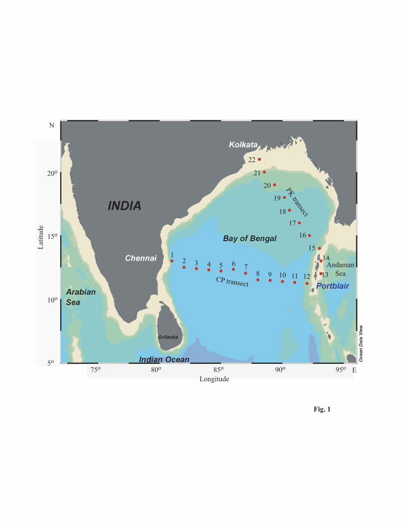
Fig. 1 Study area map showing station locations along the Chennai–Port Blair (CP) and Port Blair-Kolkata (PK)

transects in the Bay of Bengal

Fig. 2 Spatio-temporal variation in total dinoflagellate abundance (cell L-1) along the Chennai–Port Blair (CP) and

Port Blair–Kolkata (PK) transects in (a) Nov 03, (b) Feb-Mar 04, (c) Jun 04, (d) Jul-Aug 04, (e) Oct 04 and (f)

Sep 06.

Fig. 3 The percentage contribution of autotrophic, mixotrophic and heterotrophic dinoflagellates along the (a-e)

Chennai–Port Blair (CP) and (f-j) Port Blair–Kolkata (PK) transects. (a) Feb 04, (b) Jun 04, (c) Jul 04, (d) Oct 04,

(e) Sep 06, (f) Nov 03, (g) Mar 04, (h) Aug 04, (i) Oct 04 and (j) Sep 06.

Fig. 4 The five most abundant species during each sampling period at the (a) Chennai–Port Blair and (b) Port

Blair-Kolkata transects. The maximum diameter of circle corresponds to average 9 cell L-1.

AndamanSea

PK transect

CP transect

12 3 4 5 6 7

8 9 10 11 12 13

1415

16

1718

19

20

21

22

75o 80o 85o 90o 95o

LongitudeE

N

10o

5o

20o

15o

Latit

ude

Fig. 1

Longitude Longitude Longitude

Latit

ude

N

E

Latit

ude

(b) (c)

10

12

14

16

18

20

22

10

12

14

16

18

20

22

13

14

15

16

17

18

19

20

21

22

10

12

14

16

18

20

22

15

16

17

18

19

20

22

21

14

13

1 2 3 4 56 7 8 9

10 11 12

INDIAINDIA

INDIA

1 2 3 4 56 7 8 9

10 11 12

80 82 84 86 88 90 92 9410

12

14

16

18

20

22

80 82 84 86 88 90 92 9410

12

14

16

18

20

22

80 82 84 86 88 90 92 9410

12

14

16

18

20

22

15

16

17

18

19

20

22

21

14

13

1 2 4 56 7 8 9

10 11 12

3

80 82 84 86 88 90 92 9480 82 84 86 88 90 92 9480 82 84 86 88 90 92 94

15

16

17

18

19

20

22

21

14

13

1 2 3 4 56 7 8 9

10 11 12

80 82 84 86 88 90 92 9480 82 84 86 88 90 92 9480 82 84 86 88 90 92 94

15

16

17

18

19

20

22

21

14

13

1 2 3 4 56 7 8 9

10 11 12

0

10

20

30

40

50

60

70

80

90

100

(a) (b) (c)

(f)(e)(d)

Fig. 2

37

48

15

26

45

29

35

38

27

22

3543

35

46

18

4146

13

27

42

32

25

38

37

18

51

31

28

23

49

Autotrophic

Mixotrophic

Heterotrophic

(a)

(b)

(c)

(d)

(e)

(f)

(g)

(h)

(i)

(j)

Nov 03

Feb-Mar 04

Jun 04

Jul-Aug 04

Oct 04

Sep 06

CP transect PK transect

Fig. 3

b)

Feb04

Jun04

Jul04

Oct04

Sep06

Amphisolenia bidentata

Amphidinium sp.

Ceratium fusus

Ceratium pentagonum

Ceratium symmetricum

Ceratium teres

Gotoius abei

Oxytoxum globosum

Oxytoxum scolopax

Prorocentrum belizianum

Prorocentrum sp.

Protoperidinium ovatum

Protoperidinium pedunculatum

Protoperidinium sp.

Scrippsiella spp.

Scrippsiella trochoidea

a)

Oct04

Aug04

Mar04

Nov03

Sep06

Alexandrium spp.

Amphidinium sp.

Blepharocysta sp.

Ceratium extensum

Ceratium furca

Ceratium fusus

Ceratium teres

Dinophysis miles

Dinophysis spp.

Pyrocystis spp.

Gotoius abei

Noctiluca scintillans

Oxytoxum scolopax

Protoperidinium ovatum

Protoperidinium sp.

Scrippsiella spp.

Scrippsiella trochoideaFig. 4

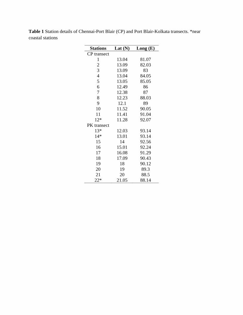
Table 1 Station details of Chennai-Port Blair (CP) and Port Blair-Kolkata transects. *near coastal stations

Stations Lat (N) Long (E) CP transect

1 13.04 81.07 2 13.09 82.03 3 13.09 83 4 13.04 84.05 5 13.05 85.05 6 12.49 86 7 12.38 87 8 12.23 88.03 9 12.1 89 10 11.52 90.05 11 11.41 91.04 12* 11.28 92.07

PK transect 13* 12.03 93.14 14* 13.01 93.14 15 14 92.56 16 15.01 92.24 17 16.08 91.29 18 17.09 90.43 19 18 90.12 20 19 89.3 21 20 88.5 22* 21.05 88.14

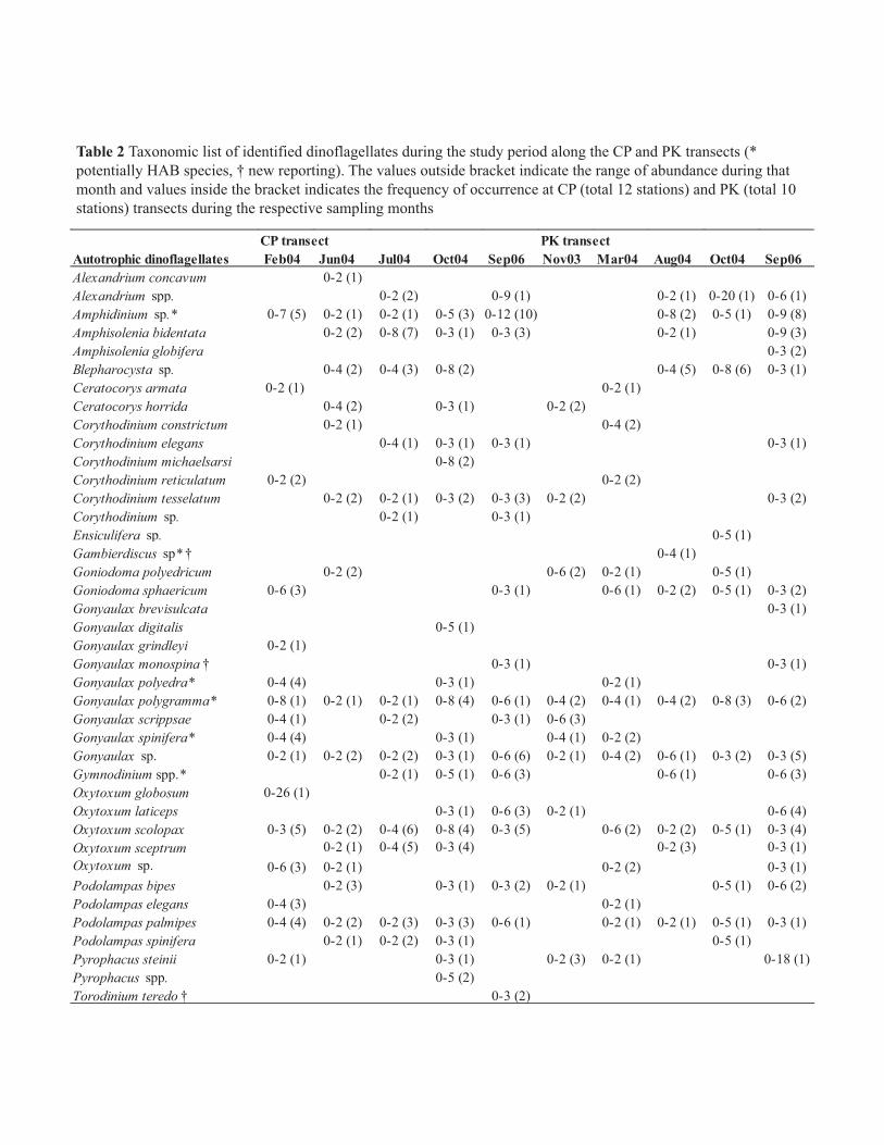
CP transect PK transectAutotrophic dinoflagellates Feb04 Jun04 Jul04 Oct04 Sep06 Nov03 Mar04 Aug04 Oct04 Sep06Alexandrium concavum 0-2 (1)Alexandrium spp. 0-2 (2) 0-9 (1) 0-2 (1) 0-20 (1) 0-6 (1)Amphidinium sp.* 0-7 (5) 0-2 (1) 0-2 (1) 0-5 (3) 0-12 (10) 0-8 (2) 0-5 (1) 0-9 (8)Amphisolenia bidentata 0-2 (2) 0-8 (7) 0-3 (1) 0-3 (3) 0-2 (1) 0-9 (3)Amphisolenia globifera 0-3 (2)Blepharocysta sp. 0-4 (2) 0-4 (3) 0-8 (2) 0-4 (5) 0-8 (6) 0-3 (1)Ceratocorys armata 0-2 (1) 0-2 (1)Ceratocorys horrida 0-4 (2) 0-3 (1) 0-2 (2)Corythodinium constrictum 0-2 (1) 0-4 (2)Corythodinium elegans 0-4 (1) 0-3 (1) 0-3 (1) 0-3 (1)Corythodinium michaelsarsi 0-8 (2)Corythodinium reticulatum 0-2 (2) 0-2 (2)Corythodinium tesselatum 0-2 (2) 0-2 (1) 0-3 (2) 0-3 (3) 0-2 (2) 0-3 (2)Corythodinium sp. 0-2 (1) 0-3 (1)Ensiculifera sp. 0-5 (1)Gambierdiscus sp* † 0-4 (1)Goniodoma polyedricum 0-2 (2) 0-6 (2) 0-2 (1) 0-5 (1)Goniodoma sphaericum 0-6 (3) 0-3 (1) 0-6 (1) 0-2 (2) 0-5 (1) 0-3 (2)Gonyaulax brevisulcata 0-3 (1)Gonyaulax digitalis 0-5 (1)Gonyaulax grindleyi 0-2 (1)Gonyaulax monospina † 0-3 (1) 0-3 (1)Gonyaulax polyedra* 0-4 (4) 0-3 (1) 0-2 (1)Gonyaulax polygramma* 0-8 (1) 0-2 (1) 0-2 (1) 0-8 (4) 0-6 (1) 0-4 (2) 0-4 (1) 0-4 (2) 0-8 (3) 0-6 (2)Gonyaulax scrippsae 0-4 (1) 0-2 (2) 0-3 (1) 0-6 (3)Gonyaulax spinifera* 0-4 (4) 0-3 (1) 0-4 (1) 0-2 (2)Gonyaulax sp. 0-2 (1) 0-2 (2) 0-2 (2) 0-3 (1) 0-6 (6) 0-2 (1) 0-4 (2) 0-6 (1) 0-3 (2) 0-3 (5)Gymnodinium spp.* 0-2 (1) 0-5 (1) 0-6 (3) 0-6 (1) 0-6 (3)Oxytoxum globosum 0-26 (1)Oxytoxum laticeps 0-3 (1) 0-6 (3) 0-2 (1) 0-6 (4)Oxytoxum scolopax 0-3 (5) 0-2 (2) 0-4 (6) 0-8 (4) 0-3 (5) 0-6 (2) 0-2 (2) 0-5 (1) 0-3 (4)Oxytoxum sceptrum 0-2 (1) 0-4 (5) 0-3 (4) 0-2 (3) 0-3 (1)Oxytoxum sp. 0-6 (3) 0-2 (1) 0-2 (2) 0-3 (1)Podolampas bipes 0-2 (3) 0-3 (1) 0-3 (2) 0-2 (1) 0-5 (1) 0-6 (2)Podolampas elegans 0-4 (3) 0-2 (1)Podolampas palmipes 0-4 (4) 0-2 (2) 0-2 (3) 0-3 (3) 0-6 (1) 0-2 (1) 0-2 (1) 0-5 (1) 0-3 (1)Podolampas spinifera 0-2 (1) 0-2 (2) 0-3 (1) 0-5 (1)Pyrophacus steinii 0-2 (1) 0-3 (1) 0-2 (3) 0-2 (1) 0-18 (1)Pyrophacus spp. 0-5 (2)Torodinium teredo † 0-3 (2)

Table 2 Taxonomic list of identified dinoflagellates during the study period along the CP and PK transects (* potentially HAB species, † new reporting). The values outside bracket indicate the range of abundance during that month and values inside the bracket indicates the frequency of occurrence at CP (total 12 stations) and PK (total 10 stations) transects during the respective sampling months

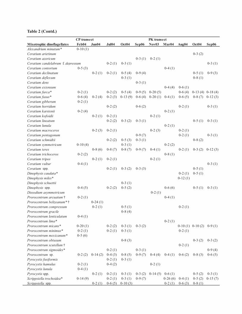
CP transect PK transectMixotrophic dinoflagellates Feb04 Jun04 Jul04 Oct04 Sep06 Nov03 Mar04 Aug04 Oct04 Sep06Alexandrium minutum* 0-10 (1)Ceratium arietinum 0-3 (2)Ceratium azoricum 0-3 (1) 0-2 (1)Ceratium candelabrum f. depressum 0-2 (1) 0-3 (1) 0-3 (1)Ceratium contortum 0-5 (3) 0-4 (1)Ceratium declinatum 0-2 (1) 0-2 (1) 0-5 (4) 0-9 (4) 0-5 (1) 0-9 (3)Ceratium deflexum 0-3 (1) 0-8 (1)Ceratium dens 0-3 (1)Ceratium extensum 0-4 (4) 0-6 (1)Ceratium furca* 0-2 (1) 0-2 (2) 0-5 (4) 0-9 (5) 0-20 (5) 0-6 (4) 0-13 (4) 0-18 (4)Ceratium fusus* 0-6 (4) 0-2 (4) 0-2 (3) 0-13 (9) 0-6 (4) 0-20 (1) 0-4 (1) 0-6 (5) 0-8 (7) 0-12 (3)Ceratium gibberum 0-2 (1)Ceratium horridum 0-2 (2) 0-6 (2) 0-2 (1) 0-3 (1)Ceratium karstenii 0-2 (4) 0-2 (1)Ceratium kofoidii 0-2 (1) 0-2 (1) 0-2 (1)Ceratium lineatum 0-2 (2) 0-3 (2) 0-3 (1) 0-5 (1) 0-3 (1)Ceratium lunula 0-2 (1)Ceratium macroceros 0-2 (3) 0-2 (1) 0-2 (3) 0-2 (1)Ceratium pentagonum 0-9 (7) 0-2 (1) 0-3 (1)Ceratium schmidtii 0-2 (2) 0-5 (3) 0-3 (1) 0-8 (2)Ceratium symmetricum 0-10 (4) 0-3 (1) 0-2 (2)Ceratium teres 0-8 (6) 0-8 (7) 0-8 (7) 0-9 (7) 0-4 (1) 0-2 (1) 0-3 (2) 0-12 (3)Ceratium trichoceros 0-2 (2) 0-8 (1)Ceratium tripos 0-2 (1) 0-2 (1) 0-2 (1)Ceratium vultur 0-4 (1) 0-3 (1)Ceratium spp. 0-2 (1) 0-3 (2) 0-3 (3) 0-5 (1)Dinophysis caudata* 0-2 (1) 0-5 (1)Dinophysis miles* 0-12 (1)Dinophysis schuettii 0-3 (1)Dinophysis spp. 0-4 (5) 0-2 (2) 0-5 (2) 0-6 (6) 0-5 (1) 0-3 (1)Dissodium asymmetricum 0-2 (1)Prorocentrum arcuatum † 0-2 (1) 0-4 (1)Prorocentrum belizeanum* † 0-24 (1)Prorocentrum compressum 0-2 (1) 0-5 (1) 0-2 (1)Prorocentrum gracile 0-8 (4)Prorocentrum lenticulatum 0-4 (1)Prorocentrum lima* 0-2 (1)Prorocentrum micans* 0-20 (1) 0-2 (2) 0-3 (1) 0-3 (2) 0-10 (1) 0-10 (2) 0-9 (1)Prorocentrum minimus* 0-2 (1) 0-2 (1) 0-3 (1) 0-2 (1)Prorocentrum mexicanum* 0-5 (6) Prorocentrum obtusum 0-8 (3) 0-3 (2) 0-3 (2)Prorocentrum scutellum † 0-2 (1)Prorocentrum sigmoides* 0-2 (1) 0-3 (1) 0-9 (4)Prorocentrum sp. 0-2 (2) 0-14 (2) 0-4 (3) 0-8 (5) 0-9 (7) 0-4 (4) 0-4 (1) 0-6 (2) 0-8 (3) 0-6 (5)Pyrocystis fusiformis 0-2 (1) 0-3 (1)Pyrocystis hamulus 0-2 (1) 0-4 (2) 0-2 (1)Pyrocystis lunula 0-4 (1)Pyrocystis spp. 0-2 (1) 0-2 (1) 0-3 (1) 0-3 (2) 0-14 (5) 0-6 (1) 0-5 (2) 0-3 (1)Scrippsiella trochoidea* 0-14 (9) 0-2 (1) 0-3 (1) 0-9 (7) 0-26 (6) 0-4 (1) 0-5 (2) 0-15 (7)Scrippsiella spp. 0-2 (1) 0-6 (5) 0-10 (3) 0-2 (1) 0-6 (3) 0-8 (1)

Table 2 (Contd.)

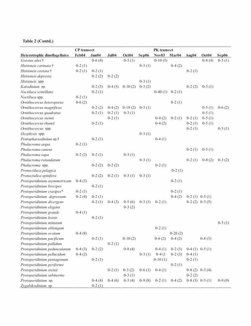
CP transect PK transectHeterotrophic dinoflagellates Feb04 Jun04 Jul04 Oct04 Sep06 Nov03 Mar04 Aug04 Oct04 Sep06Gotoius abei † 0-6 (4) 0-3 (1) 0-10 (5) 0-8 (4) 0-3 (1)Histioneis carinata † 0-2 (1) 0-3 (1) 0-4 (2)Histioneis costata † 0-2 (1) 0-2 (1) 0-2 (1)Histioneis depressa 0-2 (2) 0-2 (2)Histioneis spp. 0-3 (1)Katodinium sp. 0-2 (3) 0-4 (5) 0-10 (2) 0-3 (2) 0-2 (2) 0-5 (1)Noctiluca scintillans 0-2 (1) 0-40 (1) 0-2 (1)Noctiluca spp. 0-2 (1)Ornithocercus heteroporus 0-6 (2) 0-2 (1)Ornithocercus magnificus 0-2 (2) 0-4 (2) 0-18 (2) 0-3 (1) 0-5 (1) 0-6 (2)Ornithocercus quadratus 0-2 (1) 0-2 (1) 0-3 (1) 0-5 (1)Ornithocercus steinii 0-2 (1) 0-4 (2) 0-2 (1) 0-2 (1) 0-5 (1)Ornithocercus thumii 0-2 (1) 0-4 (2) 0-2 (1) 0-5 (1)Ornithocercus spp. 0-2 (1) 0-3 (1)Oxyphysis spp. 0-3 (1)Pentapharsodinium sp.† 0-2 (1) 0-4 (1)Phalacroma argus 0-2 (1)Phalacroma cuneus 0-2 (1) 0-5 (1)Phalacroma rapa 0-2 (2) 0-2 (1) 0-3 (1)Phalacroma rotundatum 0-3 (1) 0-2 (1) 0-8 (2) 0-3 (2)Phalacroma spp. 0-2 (2) 0-2 (2) 0-2 (1)Pronoctiluca pelagica 0-2 (1)Pronoctulica spinifera 0-2 (2) 0-2 (1) 0-3 (1) 0-3 (1)Protoperidinium asymmetricum 0-4 (3) 0-2 (1)Protoperidinium brevipes 0-2 (1)Protoperidinium crasipes* 0-2 (1) 0-2 (1)Protoperidinium depressum 0-2 (4) 0-2 (1) 0-4 (2) 0-2 (1) 0-5 (1)Protoperidinium divergens 0-2 (1) 0-4 (3) 0-5 (6) 0-3 (1) 0-2 (1) 0-2 (2) 0-3 (5)Protoperidinium elegans 0-3 (2)Protoperidinium grande 0-4 (1)Protoperidinium leonis 0-2 (1)Protoperidinium minutum 0-3 (1)Protoperidinium oblongum 0-2 (1)Protoperidinium ovatum 0-4 (8) 0-26 (2)Protoperidinium pacificum 0-2 (1) 0-10 (2) 0-6 (2) 0-4 (2) 0-8 (3)Protoperidinium pallidum 0-2 (1)Protoperidinium pedunculatum 0-4 (3) 0-2 (2) 0-8 (4) 0-4 (1) 0-2 (3) 0-4 (1) 0-5 (1)Protoperidinium pellucidum 0-4 (2) 0-3 (1) 0-4 (1 0-2 (3) 0-4 (1)Protoperidinium pentagonum 0-2 (1) 0-10 (1) 0-2 (1)Protoperidinium pyriforme 0-2 (1)Protoperidinium steinii 0-2 (1) 0-3 (2) 0-6 (1) 0-4 (1) 0-8 (2) 0-3 (4)Protoperidinium subinerme 0-3 (1) 0-2 (2)Protoperidinium sp. 0-4 (4) 0-4 (6) 0-3 (4) 0-9 (8) 0-2 (1) 0-4 (2) 0-8 (3) 0-5 (1) 0-9 (9)Zygabikodinium sp. 0-2 (1)

Table 2 (Contd.)

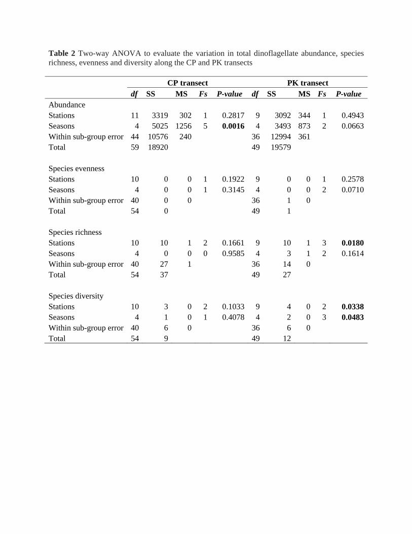
Table 2 Two-way ANOVA to evaluate the variation in total dinoflagellate abundance, species richness, evenness and diversity along the CP and PK transects CP transect PK transect df SS MS Fs P-value df SS MS Fs P-value Abundance Stations 11 3319 302 1 0.2817 9 3092 344 1 0.4943Seasons 4 5025 1256 5 0.0016 4 3493 873 2 0.0663Within sub-group error 44 10576 240 36 12994 361 Total 59 18920 49 19579 Species evenness Stations 10 0 0 1 0.1922 9 0 0 1 0.2578Seasons 4 0 0 1 0.3145 4 0 0 2 0.0710Within sub-group error 40 0 0 36 1 0 Total 54 0 49 1 Species richness Stations 10 10 1 2 0.1661 9 10 1 3 0.0180Seasons 4 0 0 0 0.9585 4 3 1 2 0.1614Within sub-group error 40 27 1 36 14 0 Total 54 37 49 27 Species diversity Stations 10 3 0 2 0.1033 9 4 0 2 0.0338Seasons 4 1 0 1 0.4078 4 2 0 3 0.0483Within sub-group error 40 6 0 36 6 0 Total 54 9 49 12