DIMENSION REDUCTION FOR CENSORED REGRESSION DATA

The Annals of Statistics1999, Vol. 27, No. 1, 1�23

DIMENSION REDUCTION FOR CENSOREDREGRESSION DATA

BY KER-CHAU LI,1 JANE-LING WANG2 AND CHUN-HOUH CHEN

University of California, Los Angeles, University of California, Davisand Academia Sinica, Taiwan

Without parametric assumptions, high-dimensional regression analy-sis is already complex. This is made even harder when data are subject tocensoring. In this article, we seek ways of reducing the dimensionality ofthe regressor before applying nonparametric smoothing techniques. If thecensoring time is independent of the lifetime, then the method of slicedinverse regression can be applied directly. Otherwise, modification isneeded to adjust for the censoring bias. A key identity leading to the biascorrection is derived and the root-n consistency of the modified estimate isestablished. Patterns of censoring can also be studied under a similardimension reduction framework. Some simulation results and an applica-tion to a real data set are reported.

1. Introduction. Survival data are often subject to censoring. When thisoccurs, the incompleteness of the observed data may induce a substantial biasin the sample. Several approaches have been suggested to overcome theassociated difficulties in regression, including the accelerated failure timemodel, censored linear regression, the Cox proportional hazard model andmany others. Survival analysis becomes even more intricate when the dimen-sion of the regressor increases. To apply any of the aforementioned methods,users are required to specify a functional form which relates the outcomevariables to the input ones. However, in reality, knowledge needed for anappropriate model specification is often inadequate. As a matter of fact, theacquisition of such information may well turn out to be one of the primarygoals of the study itself. Under such circumstances, it seems preferable tohave exploratory tools that rely less on such model specification. This is theissue to be addressed in this article. The dimension reduction approach of LiŽ .1991 will be extended to settings which allow for censoring in the data. Weshall offer methods of finding low-dimensional projections of the data forvisually examining the censoring pattern. We shall show how censoredregression data can still be analyzed without assuming the functional form apriori.

Received January 1997; revised September 1998.1 Supported in part by an NSF grant and a Guggenheim Fellowship. Part of the research was

carried out while visiting the Institute of Statistical Science, Academia Sinica, Taiwan, in 1994with support from the National Science Council, Taiwan, R.O.C.

2 Supported in part by NSF Grant DMS-93-12170.AMS 1991 subject classifications. 62G05, 62J20.Key words and phrases. accelated failure time model, censored linear regression, Cox model,

curse of dimensionality, hazard function, Kaplan-Meier estimate, regression graphics, slicedinverse regression, survival analysis

1

K.-C. LI, J.-L. WANG AND C.-H. CHEN2

Dimensionality sets a severe limitation even in the exploratory stage ofdata analysis. This is true even without the presence of censoring. Forexample, when the dimension is one or two, a two-dimensional or three-dimensional scatterplot of the response variable against the regressor ishelpful in obtaining general ideas about the shape of the regression function,the pattern of heterogeneity and other valuable structural information. How-ever, as the dimension increases, the total number of two-dimensional orthree dimensional scatterplots escalates quickly. Very soon this task couldturn into an extremely laborious exercise. Without proper guidance, it maynot be easy for us to put together a clear global picture about the data fromvarious plots. How to bypass the curse of dimensionality has been an impor-

Ž .tant issue; see, for example, Huber 1985 .Li’s framework for dimension reduction in regression begins with the

following formulation:

1.1 Y � g � � x, . . . , � � x, � .Ž . Ž .1 k

Ž .The main feature of 1.1 is that g is completely unknown and so is thedistribution of � , which is independent of the p-dimensional regressor x.

Ž .When k is smaller than p, 1.1 imposes a dimension reduction structure byclaiming that the dependence of Y on the p-dimensional x only comes fromthe k variates, � � x, . . . , � � x, but the functional form of the dependence1 kstructure is not specified. The k-dimensional space spanned by the k� vectors

Ž .is called the e.d.r. effective dimension reduction space and any vector in thisspace is referred to as an e.d.r. direction. The primary goal of Li’s approach isto estimate the e.d.r. directions so that we can plot y against the e.d.r.variates for visually exploring the structure of the regression and for moreeffectively applying various low-dimensional regression techniques to thereduced space. The notion of e.d.r. space and its role in regression graphics

Ž . Ž .are further explored in Cook 1994 and Cook and Weisberg 1994 .To incorporate censoring into the dimension reduction framework, let

Y o � the true unobservable lifetime,Ž .C � the censoring time,

� � the censoring indicator; � � 1, if Y o � C and � � 0, otherwise,

� o 4Y � min Y , C , the observed time.

We assume that

1.2 Y o follows model 1.1 ;Ž . Ž .1.3 Conditional on x, C is independent of Y o .Ž .

Ž .The observed sample consists of n i.i.d. observations, Y , x , � , i � 1, . . . , ni i iŽ . ofrom the distribution of Y, x, � . The continuous random variables, Y , C,

Ž .are not observed. Condition 1.3 is the usual independence assumption toŽ .ensure identifiability under the random censoring scheme. If 1.3 is violated,

then one needs more information on the censoring mechanism to build anappropriate model. This is not considered in this paper.

DIMENSION REDUCTION FOR CENSORED REGRESSION DATA 3

For k � 1, our formulation may include the generalized linear model� Ž .� �McCullagh and Nelder 1989 and the linear transformation model DoksumŽ .�1987 as special cases. The latter also includes several survival analysismodels such as the accelerated failure time model, the proportional hazard

�model, the proportional odds model and the logit and probit models DoksumŽ .�and Gasko 1990 .

Ž .Without censoring, sliced inverse regression SIR is a simple method forŽ .finding the e.d.r. space. Instead of directly estimating E Y � x , a p-dimen-

sional surface, the roles of x and Y are reversed�the focus turns to theŽ . pinverse regression E x � Y , which is a curve in R . Under appropriate

� Ž .�conditions Lemma 3.1 of Li 1991 , the inverse regression curve is shown tofall into a k-dimensional subspace. In particular, when the regressor distribu-tion has mean zero and with the identity covariance, this k-dimensionalsubspace coincides with the e.d.r. space. Exploring this connection, SIR beginswith a simple estimate of the inverse regression curve by partitioning thedata into several slices according to the Y values and computing the mean ofx within each slice; this is the slicing step. It is then followed by aneigenvalue decomposition step�a principal component type of analysis in-tended to locate the subspace containing the inverse regression curve. See LiŽ .1991 for further details. Properties of SIR have been studied in several

Ž . Ž .places: Carroll and Li 1992, 1995 , Chen and Li 1998 , Cook and WeisbergŽ . Ž . Ž . Ž .1991, 1994 , Duan and Li 1991 , Hsing and Carroll 1992 , Schott 1994 ,

Ž .Zhu and Ng 1995 .How does censoring affect SIR? This depends on the relationship between

the censoring time C and the regressor x. Section 2 considers the indepen-dence case in which1.4 C is independent of x and Y o .Ž .

We show that the general theory of SIR is applicable without modificationand the directions found by SIR are still consistent. Thus for the indepen-dence case, censoring does not introduce bias to the SIR estimates.

However, SIR will be affected by other censoring mechanisms that do notŽ .follow 1.4 . In Section 3, we introduce a general strategy to overcome this

difficulty. The proposed approach is to introduce a suitable weight functionfor the censored observations for offsetting bias in estimating the slice means.The weight function can be estimated by nonparametric estimation tech-niques for conditional survival functions. For simplicity, the kernel method isused and we establish the root-n consistency for the modified SIR.

In Section 4, we bring out a dimension reduction setting for studying theŽ .pattern of censoring when the independent censoring condition 1.4 is vio-

lated. We argue for the importance of visualizing the heavy censoring region,a nontrivial task in the high-dimensional situation. Data analysts have torecognize this region because heavy censoring sets severe limitations infinding the structure of regression. The dimension reduction assumption on C

Ž .is a natural counterpart of 1.2 ,1.5 C � h � � x, . . . , � � x, � � .Ž . Ž .1 c


Ž . Ž .Then 1.2 and 1.5 together allow us to treat the survival time andcensoring time equivalently. But to avoid confusion, we shall refer to � ’s anditheir linear combinations as e.d.r. censoring directions. In contrast, the e.d.r.directions for Y o will be called e.d.r. lifetime directions. Both censoring andlifetime directions as well as their linear combinations will be called jointe.d.r. directions. We show how to estimate the joint e.d.r. directions through adouble slicing procedure.

From the joint e.d.r. directions, we can recover the e.d.r. lifetime directionsby further applying the modified SIR strategy of Section 3. This is illustratedin Section 5. The performance of the procedure is examined through twosimulation studies. We apply our method to a data set about the study of

Ž .primary biliary cirrhosis PBC at the Mayo Clinic. Section 6 concludes thisarticle by summarizing our findings. Some questions are raised for furtherstudy.

( )2. SIR under the independence assumption 1.4 . Denote the uncen-oŽ o. Ž o o.sored inverse regression curve by � y � E x � Y � y . Without censoring

Ž o.i.e., Y � Y , the population version of SIR is based on the following eigen-value decomposition:

o b � b ,� i i x i

� �� ,1 p2.1Ž .

where2.2 o � cov E x � Y oŽ . Ž .Ž .�

and � cov x .Ž .x

The justification for using the first k eigenvectors b with nonzero eigen-iŽ .values to estimate the e.d.r. lifetime directions follows from Lemma 3.1 of Li

Ž .1991 , which can be stated as follows.

Ž .LEMMA 2.1. Assume that the dimension reduction assumption 1.2 holds.o �1Ž oŽ . Ž .. Ž .Then for any y , � y � E x falls into the e.d.r. lifetime space underx

the condition that

2.3 for any vector b , E b�x � � � x, . . . , � � x is linear .Ž . Ž .1 k

Ž .Design condition 2.3 has been discussed in several places. The perfor-mance of SIR is not very sensitive to this condition; see the discussion and

Ž . Ž . Ž .the rejoinder of Li 1991 , Cook 1994 , Cook and Weisberg 1991, 1994 .Ž .Carroll and Li 1995 . In view of the fact that most low-dimensional projec-

�tions of high-dimensional data often appear like normal distributions Di-Ž .� Ž .aconis and Freedman 1984 , Hall and Li 1993 argue for the generality of

this condition in high-dimensional situations. On the other hand, reweightingŽ .and subsampling methods can also be applied to achieve 2.3 : Brillinger

Ž . Ž .1991 , Cook and Nachtsheim 1994 . Further discussion on this condition canŽ .be found in Li 1997 .


Censoring alters the distribution of the observed time Y. Its effect on SIRŽ .can be studied by comparing the censored inverse regression curve � y �

Ž . oŽ o.E x � Y � y with the uncensored one � y . By conditioning, we have

2.4 E x � Y � y � E E x � Y o , C � Y � y .Ž . Ž . Ž .Ž .Ž . Ž o . Ž o.Under 1.4 , E x � Y , C is equal to E x � Y , implying that

2.5 E x � Y � y � E � o Y o � Y � y .Ž . Ž . Ž .Ž .oŽ o.Since Lemma 2.1 applies to � y , the following result is obtained.

Ž . Ž . �1Ž Ž . Ž ..LEMMA 2.2. Assume that 1.2 and 1.4 hold. Then � y � E xxŽ .falls into the e.d.r lifetime space under 2.3 .

Ž . Ž .To implement SIR on the data Y , x , i � 1, . . . , n, we follow Li 1991 .i iFirst we partition y� s into H intervals, I , h � 1, . . . , H. Then for eachi hinterval, we compute the partition slice mean x by averagingh

1x � x ,Ýh inh x �Ii h

where n is the number of cases falling into I . Then the covariance matrixh h

H nh ˆx � x x � x � � Ž . Ž .Ý h h �nh�1

is formed. Finally we conduct the eigenvalue decomposition

ˆ ˆ ˆ ˆ b � b ,� i i x i

ˆ ˆ � �� .1 p

Ž .With Lemma 2.2 and following the argument in Li 1991 , we obtain theˆroot-n consistency of SIR estimates b for finding e.d.r. lifetime directions.i

Thus censoring does not introduce bias to SIR. However, this is true onlywhen the censoring time is independent of the regressors and the true

Ž .lifetime. Without 1.4 , this appealing result vanishes and substantial biasŽ .may be induced by censoring under the more general condition 1.3 .

( )3. A strategy for modifying SIR under 1.3 . An ideal way of bypass-Ž .ing the difficulties caused by general censoring 1.3 is to slice the true

survival time Y o. At first sight, this does not appear feasible because undercensoring, Y o is unobservable. The promise comes from an identity derived inSection 3.1, which relates the conditional expectation of x in each slice to theobserved time Y and the censored indicator. This leads to a modified slicingstep by a suitable weighting scheme for offsetting the censoring bias inestimating the slice means. The consistency of this new procedure is dis-cussed in Section 3.2.


3.1. An identity. Let 0 � t � t � �� t � � � t be a partition on1 2 H H1� othe survival time. The expected value of x in a slice, m � E x � Y �j

� .4t , t , can be written asj j1

o o oE x1 Y � t , t . E x1 Y � t � E x1 Y � t½ 5Ž . � 4 � 4Ž . Ž .j j1 j j13.1 m � � ,Ž . j o oo E 1 Y � t � E 1 Y � tP Y � t , t � 4 � 4Ž . Ž ..� 4 j j1j j1

Ž .where 1 � is the indicator function. The two numerator terms take the sameŽ o .form, which involves the unobservable indicator 1 Y � t . They can be

converted into terms with Y and � via the identity,

3.2 E x1 Y o � t � E x1 Y � t E x1 Y � t , � � 0 w Y , t , x ,� 4 � 4 � 4Ž . Ž . Ž . Ž . Ž .

where for t� � t,

So t � xŽ .3.3 w t�, t , x � ,Ž . Ž . oS t� � xŽ .

o � o 4S t � x � P Y � t � xŽ .3.4Ž .

� conditional survival function for Y o , given x.

Consider the plane of variables Y o and C in Figure 1. The integrationo Žregion Y � t is decomposed into two parts. The first region area I in Fig-

. oure 1 with Y � t, C � t or equivalently, Y � t, contributes to the first termŽ . oon the right side of 3.2 . The second region with Y � t, C � t, falls into the

Žcensored area, � � 0. It is contained in the larger region dashed area II in. Ž .Figure 1 with Y � t and � � 0. The second term on the right side of 3.2

comes from integration over this larger region with the weight adjustment

FIG. 1. Integration regions.


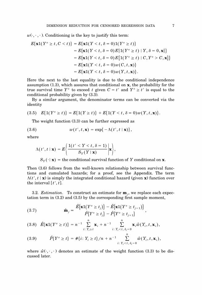
Ž .w �, � , � . Conditioning is the key to justify this term:

E x1 Y o � t , C � t � E x1 Y � t , � � 0 1 Y o � t� 4 � 4Ž . Ž . Ž .o� E x1 Y � t , � � 0 E 1 Y � t � Y , � � 0, x� 4Ž . Ž .o o� E x1 Y � t , � � 0 E 1 Y � t � C , Y � C , x� 4Ž . Ž .

� E x1 Y � t , � � 0 w C , t , x� 4Ž . Ž .� E x1 Y � t , � � 0 w Y , t , x .� 4Ž . Ž .

Here the next to the last equality is due to the conditional independenceŽ .assumption 1.3 , which assures that conditional on x, the probability for the

true survival time Y o to exceed t given C � t� and Y o � t� is equal to theŽ .conditional probability given by 3.3 .

By a similar argument, the denominator terms can be converted via theidentity

3.5 E 1 Y o � t � E 1 Y � t E 1 Y � t , � � 0 w Y , t , x .� 4 � 4 � 4Ž . Ž . Ž . Ž . Ž .

Ž .The weight function 3.3 can be further expressed as

3.6 w t�, t , x � exp � t�, t � x ,� 4Ž . Ž . Ž .where

1 t� � Y � t , � � 1Ž . t�, t � x � E x ,Ž . ½ 5S Y � xŽ .Y

S �� x � the conditional survival function of Y conditional on x.Ž .Y

Ž .Then 3.6 follows from the well-known relationship between survival func-tions and cumulated hazards; for a proof, see the Appendix. The termŽ . Ž . t�, t � x is simply the integrated conditional hazard given x function over

� �the interval t�, t .

3.2. Estimation. To construct an estimate for m , we replace each expec-jŽ . Ž .tation term in 3.2 and 3.5 by the corresponding first sample moment,

ˆ o ˆ oE x1 Y � t � E x1 Y � t� 4 � 4Ž . Ž .j j13.7 m � ,Ž . ˆ j o oˆ ˆP Y � t � P Y � t� 4 � 4j j1

n no �1 �1ˆ3.8 E x1 Y � t � n x n x w Y , t , x ,� 4Ž . Ž . Ž .ˆÝ Ýi i i i

i : Y �t i : Y �t , � �0i i i

no �1� 4 � 43.9 P Y � t � � i : Y � t n n w Y , t , x ,Ž . Ž .ˆÝi i i

i : Y �t , � �0i i

Ž . Ž .where w �, � , � denotes an estimate of the weight function 3.3 to be dis-ˆcussed later.


Ž .After estimating each slice mean by 3.7 , we can form the covariancematrix of the slice means in the usual way;

� m � x m � x �p ,ˆ ˆ ˆŽ . Ž .Ý� j j joj

ˆ o ˆ op � P Y � t � P Y � t .� 4 � 4ˆj j j1

Finally, we may conduct the eigenvalue decomposition as before to find theSIR directions

ˆ ˆo ˆ ˆ ˆoo b � b ,� i i x i

3.10Ž .ˆ ˆ � �� .1 p

Ž .Smoothing is needed in estimating w t�, t, x . There are several ways toproceed. For example, we can apply Beran’s estimates for conditional survival

Ž .functions and their variants. Under appropriate conditions, Beran 1981 andŽ .Dabrowska 1987, 1992 established the consistency of their estimates at

Ž .convergence rates slower than the root n rate similar to those commonlyfound in nonparametric regression. These consistency results lead to the

ˆ oconsistency of m as an estimate of m . It is easy to see that is alsoˆ h h �

Ž .consistent for the covariance matrix of the slice means m s. As in Li 1991 ,hˆwe can apply Lemma 2.1 to establish the consistency of b as estimates ofi

e.d.r. lifetime directions.Despite the slow rate of convergence in estimating conditional survival

� Ž .�functions hence the weight 3.3 , it is still possible to establish the root nconvergence for m . We only consider the kernel smoothing method here forˆ h

Ž . psimplicity. Let K � be a kernel function on R and h be the bandwidth inp nŽ . peach coordinate. We shall assume that h � o 1 and nh tends to infinity.n n

Ž .Further constraints will be imposed later. It is common for K � to take apŽ . Ž . Ž .product form, K x , . . . , x � K x �� K x , for some one-dimensionalp 1 p 1 pŽ . Ž .kernel function K � . Our kernel estimate of 3.6 is defined by setting

�1�1 n �p �1ˆn Ý S Y � x h K h x �xŽ . Ž .Ž .Ž .i : t �� Y � t , � �1 Y i i n p n ii iˆ3.11 t�, t � x � ,Ž . Ž .f xŽ .

n�1Ýn h�pK h�1 x � xŽ .Ž .j : Y � Y n p n j ij iˆ3.12 S Y � x � ,Ž . Ž .Y i i f xŽ .in

�1 �p �1ˆ3.13 f x � n h K h x � x .Ž . Ž . Ž .Ž .Ý n p n ii

A sketch proof of the following claim together with the regularity condi-tions needed is given in the Appendix.

Ž . Ž . Ž . Ž .LEMMA 3.1. Under the regularity conditions B.1 , B.3 , B.5 and B.8 ,given in the Appendix, m is a root-n consistent estimate for m , h � 1, . . . , H.ˆ h h


Ž .We can use this lemma and follow the same argument as in Li 1991 toshow that the modified SIR is root-n consistent. This is stated in the followingtheorem. The proof is omitted.

ˆTHEOREM 3.2. Under the assumption of Lemma 3.1, each b is a root-nhconsistent estimate for an e.d.r. direction.

Ž . Ž .Assume that f � and S �� x are d-times continuously differentiable andi Ž .that the kernel function satisfied the moment conditions Hx K x dx � 0 forp

d Ž .i � 1, . . . , d � 1, and Hx K x dx is nonzero. Then the regularity assump-ptions in Lemma 3.1 can be satisfied with bandwidth H � n�12 d providedp � d.

What we have presented so far in this section is a general strategy foroffsetting the bias due to censoring. The theoretical result of Theorem 3.2,however, may not help much in practice. The problem is that kernel smooth-ing only works well in the low-dimensional case. Thus, before applying thekernel method in estimating the weight function, we may want to reduce thedimensionality first. This is to be discussed in the next two sections.

4. Dimension reduction model for censoring time. Analyzing thecensoring pattern is an important step in studying the censored data. It helpsthe recognition of the information-poor region in x, the region where censor-ing is heavy and the regression structure is thus harder to explore. Some-times such an analysis may even become a primary part of the study. In someindustrial applications, Y o may be the potential yield of a production processand censoring C may occur because of machine malfunctioning, for example.In addition to learning how various input variables x may affect the potentialyield, quality control engineers may equally be interested in how they affectthe censoring rate; they need such knowledge to prevent machine malfunc-tioning as much as possible.

Like its counterpart Y o, we now assume that the censoring time C alsoŽ .has a dimension reduction structure given by 1.5 . Again, the functional form

of h and the distributional form of � � are both unspecified. This modelsuggests only that the dimension of the regressor can be reduced from p to c.The relationship between the e.d.r. space for the censoring time and the e.d.r.space for the true lifetime is arbitrary. They can be either identical, partlyoverlapped, or disjoint. Linear combinations of their elements form a spacewhich will be called the joint e.d.r. space. If Y o and C were used for slicing,then by the same argument used in deriving Lemma 2.1, it is easy to see that

4.1 �1 E x � Y o , C � E x falls into the joint e.d.r. space.Ž . Ž . Ž .Ž .x

Ž o .However, instead of Y , C , we can only observe Y and � . This suggestsŽ . Žthat Y and � can be used simultaneously for slicing. Let � Y, 0 � E x � Y �d

. Ž . Ž . Ž .y, � � 0 , and � Y, 1 � E x � Y � y, � � 1 . We may replace 2.1 withd

Cov � Y , � b � b ,Ž .Ž .d i i x i

� �� .1 p

4.2Ž .


Ž . Ž Ž o . .. Ž .By conditioning, E x � Y, � � E E x � Y , C � Y, � . Thus from 4.1 , we seethat

�1 � y , � � E x falls into the joint e.d.r. space.Ž . Ž .Ž .x d

Ž .This justifies the use of eigenvectors from 4.2 to estimate the joint e.d.r.space.

Ž .The sample version of 4.2 is easy to carry out. Denote the number of slicesŽ .for the uncensored � � 1 observations by H . Let I , j � 1, . . . , H be a1 1 j 1

partition of the positive real line into nonoverlapping intervals. Similarly,Ž .denote the number of slices for the censored � � 0 observations by H , and0

let I � , j � 1, . . . , H be another partition of the positive real line. We first0 j 0form the individual slice means by taking

n�1

x � np x 1 � � l , Y � I ,ˆ Ž .Ž . Ýl j l j i i i l ji�1

where p is the proportion of cases with � � l falling into interval I . Thenˆl j i l jˆ Žwe compute the covariance matrix for the slice means, � Ý Ý p x �ˆd l j l j l j

.Ž .x x � x . Finally we conduct the eigenvalue decompositionl j

ˆ ˆ ˆ ˆ ˆ b � b ,d di di x di4.3Ž .

ˆ ˆ � �� .d1 d p

Ž .Li 1991 proposed a chi-squared test for determining the number ofsignificant e.d.r. directions obtained by SIR. It should be clear that we can usethe same test for the double slicing case.

So far we have only located the joint e.d.r. directions. We shall show in thenext section how to use the procedure in Section 3 to recover the e.d.r.lifetime directions. Likewise, we can also recover the e.d.r. directions forcensoring time by exchanging the roles of censoring time and lifetime. Beforewe proceed, an example is given below to illustrate the double slicing proce-dure discussed in this section.

Ž .EXAMPLE 4.1. Take p � 6 and let x � x , . . . , x � be generated from the1 6standard normal distribution. Suppose

o � �Y � 4 � x � 1 � � ,Ž .1 1 1

C � 3 � � for x � 0, x x � 0,2 2 1 2 3

� 10 otherwise,where � � � � 0.1. Here � , � are normal random variables. Generate 3001 2 1 2cases. Sixty-six observations in the data set are censored. Now apply doubleslicing with the number of slices equal to 5 and 10, respectively, for thecensored and the uncensored groups. The eigenvalues of SIR are found to be

ˆ0.76, 0.35, 0.08, 0.06, . . . , indicating that the first two eigenvectors, b �d1ˆŽ . Ž1.14, 0.05, �0.03, �0.00, �0.04, 0.04 � and b � �0.06, 0.69, 0.74, �0.02,d2

.�0.10, �0.05 � are important. This is confirmed by the chi-squared test in LiŽ .1991 .


'Ž . Ž .Ž .The joint e.d.r. directions 1, 0, 0, 0, 0, 0 � and 1 2 0, 1, 1, 0, 0, 0 � areˆ ˆcaptured successfully by b and b . The censored cases are found to clusterd1 d2

Ž .in the first quadrant in the plot of the first two SIR variates; see Figure 2 c .Statistical information about the behavior of the true lifetime in that regionis very sparse.

5. Implementation of modified SIR. The directions found by doubleslicing can be used to relieve the difficulties encountered in Section 3 when

Ž .kernel smoothing is to be applied for estimating the weight function 3.3 .Under the dimension reduction assumptions for both the true lifetime and

Ž . Ž .the censoring time, 1.2 and 1.5 , it is easy to see that the dependence of theŽ .weight function 3.3 on x is only through joint e.d.r. variates. This suggests

the following two-stage procedure:

ˆŽ .1. Apply double slicing on Y, � and find the joint e.d.r. directions, b . Letdiˆ ˆ ˆŽ .B � b , . . . , b be the matrix formed by the first r significant direc-r d1 drtions.

�2. Apply r-dimensional kernel smoothing on B x, to obtain the weightrfunction w,ˆ

ˆ5.1 w t�, t , x � exp � t�, t � x ,Ž . Ž . Ž .� 4ˆ

where

t�, t � xŽ .�1�1 n �r �1ˆ ˆn Ý S Y � x h K h B x � xŽ . Ž .Ž . Ž .ž /i : t �� Y � t , � �1 Y i i n r n r ii i� ,

f xŽ .

5.2Ž .

Ž .FIG. 2. Three-dimensional scatterplot of Y against the first SIR variate x-axis and the secondŽ .SIR variate z-axis found by double slicing. The highlighted points are censored.


�1 n �r �1 ˆn Ý h K h B x � xŽ .ž /ž /j : Y � Y n r n r j ij iˆ5.3 S Y � x � max , c ,Ž . Ž .Y i i ½ 5f xŽ .in

�1 �r �1ˆ ˆ5.4 f x � n h K h B x � x .Ž . Ž . Ž .Ž .Ž .Ý n r n r ii

Ž .Note that a small positive number c set to 0.05 in our examples is used toˆ Ž .bound S Y � x away from zero. This is needed in order to increase theY i i

ˆ �1Ž . Ž .stability of the factor S Y � x in 5.2 . After estimating the weightY i iŽ . Ž .function, we can apply 3.7 � 3.9 and then carry out the eigenvalue decom-

Ž .position 3.10 to obtain estimates of e.d.r. lifetime directions.We first report two simulation studies to illustrate how this strategy

works. Then we apply our method to a data set concerning a study of primaryŽ .biliary cirrhosis in the liver PBC .

Ž .EXAMPLE 5.1. We take p � 6 and generate x � x , . . . , x � from the1 6standard normal distribution. The true survival time Y o and the censoringtime C are generated from

log � log �1 2oY � � ; C � � ,x x1 2� �

� �where � , � are independent uniform random variables from 0, 1 . Condi-1 2tional on x, Y o and C are seen to follow the exponential distributions withthe natural parameters , linking to x via � � x1; � � x 2 , respec-1 2 1 2tively.

Ž .We obtain 300 independent observations of Y, � ; among them, 138 casesare censored. We proceed with the SIR analysis. First, the method of double

Ž .slicing on Y and � as described by 4.3 gives eigenvalues 0.34, 0.27, 0.05, . . . .ˆ Ž .The first two eigenvectors, b � �0.67, �0.70, �0.08, 0.06, 0.11, 0.15 � andd1

ˆ Ž .b � 0.69, �0.73, 0.12, �0.04, �0.10, �0.12 �, are close to the joint e.d.r.d2space for Y o and C. We use these two directions to reduce the x dimension

Ž .before estimating the weight function w �, � , � . With the weight adjustmentŽ . Ž . Ž .given by 5.1 , we perform SIR as described by 3.7 � 3.10 to find the e.d.r.

lifetime directions. The eigenvalues are 0.40, 0.10, 0.03, . . . , and the leadingˆo ˆoŽ .eigenvector is b � �0.92, �0.12, �0.21, 0.08, 0.25, 0.11 �. We see that b is1 1

Ž .quite close to the true e.d.r. lifetime direction 1, 0, . . . , 0 �.For comparison, we also carry out the SIR analysis on Y without weight

adjustment as if the censoring were independent of x. The first directionŽ .�0.68, �0.69, �0.058, 0.07, 0.13, 0.08 � does have a substantial bias.Therefore the weight adjustment is crucial in this example.

We used the bivariate normal kernel function here and the bandwidth isset at 0.18. The sensitivity to the bandwidth choice seems mild.

EXAMPLE 5.2. Important prognostic variables affecting the hazard ratemay be different at different survival stages. In this example, we assume thatthe true survival time Y o follows an exponential distribution with the


TABLE 1The first three eigenvectors and eigenvalues of SIRfor Example 5.2 with the double slicing procedure

Ž .First vector �0.93, �0.11, 0.03, 0.03, 0.04, �0.06

Ž .Second vector 0.09, �0.76, �0.60, �0.01, 0.03, �0.13

Ž .Third vector �0.10, 0.55, �0.73, �0.03, �0.02, 0.27

Ž .Eigenvalues 0.52, 0.21, 0.15, 0.03, 0.01, 0.01

natural parameter equal to � 2 x1 until time � � log 2. From time � on, theadditional survival time follows the exponential distribution with the naturalparameter � 3 x 2. More specifically, we assume

Y * � exponential with parameter � � 2 x1 ,

Y ** � exponential with parameter � � 3 x 2 ,

Y o � Y *1 Y * � � � Y ** 1 Y * � � .Ž . Ž . Ž .

The censoring time C follows an exponential distribution with parameterequal to � x3�1 .

Ž .Again 300 independent observations of Y, � are obtained. Among them,98 cases are censored. The output of the double slicing procedure is given inTable 1. The first three eigenvectors, which have relatively larger eigenvaluescompared to the rest, are then used in estimating the weight function forfinding the true e.d.r. lifetime directions. After the weight adjustment, thefinal output of SIR is given in Table 2. Now we see that only the first twoeigenvectors stand out and the important variables x and x can be1 2identified.

EXAMPLE 5.3. The PBC data set collected at the Mayo Clinic between1974 and 1986 has been analyzed in the literature. The data set and a

Ž .detailed description can be found in Fleming and Harrington 1991 . Thereare originally seventeen regressors. Fleming and Harrington selected five ofthem in their final equation for fitting a Cox proportional model. These five

Ž .regressors plus another variable, the platelet count x below , will be used in5this illustration:

Y � number of days between registration and the earlier of death orcensoring;

� � 1 if Y is due to death; 0 otherwise;x � age in years;1

x � presence of edema;2

x � serum bilirubin, in mgdl;3

x � albumin, in gmdl;4


TABLE 2The first two eigenvectors and eigenvalues of SIR

for final result of Example 5.2 with weight adjustment

Ž .First vector �0.97, �0.15, 0.10, �0.04, 0.10, �0.15

Ž .Second vector 0.16, �0.95, �0.18, �0.02, �0.06, �0.20

Ž .Eigenvalues 0.66, 0.34, 0.05, 0.04, 0.02, 0.02

x � platelet count;5

x � prothrombin time.6

Cases with missing values are ignored and there are 308 cases remaining.We first apply double censoring with slice numbers H � H � 10. The first1 0two directions are significant, as judged from the sequence of output eigenval-ues 0.55, 0.15, 0.05, 0.0, 0.0, 0.0. Figure 3 shows the scatterplot of the first twoSIR variates. Two outliers labeled as 104 and 276 are found from the

Ž .three-dimensional plot not shown here of Y against the first two SIRvariates. They are removed. We apply double slicing again to the remaining306 cases. The SIR output essentially remains the same. This suggests thatthe dimension of the joint e.d.r. space is two.

We proceed to find the true e.d.r. lifetime directions. We take r � 2 and usethe two SIR directions reported in Table 3 to reduce the x dimension beforeestimating the weight function. The kernel function and the bandwidth arethe same as in Example 5.1. The output of the weighted SIR is given in

ˆoTable 4. Judging from the eigenvalue sequence, the first direction b is1

FIG. 3. Scatterplot of the first two SIR variates found by double slicing. �� observed, square �censored cases.


TABLE 3The first two eigenvectors and eigenvalues of SIR

for the PBC data in Example 5.3

Ž .First vector 0.02, 1.04, 0.10, �0.50, �0.00, 0.39

Ž .Second vector 0.02, �1.62, 0.17, �0.97, �0.00, �0.87

Ž .Eigenvalues 0.54, 0.16, 0.05, 0.01, 0.00, 0.00

clearly important. The second direction is also worth further examination.ˆo� ˆo�Ž . Ž .Figure 4 a and b show the scatterplots of Y against b x and against b x.1 2

Ž .Earlier analysis in Fleming and Harrington 1991 yields that the truelifetime depends on x through the variate Q � 0.0333x 0.7847x 1 20.8792 log x � 3.0553 log x 3.0157 log x . This variate turns out highly3 4 6

�oˆ 'correlated with the first SIR variate b x; the correlation coefficient is 0.858 .1� �o oˆ ˆ 'The correlation between Q and 1.3b x � 0.25b x is equal to 0.89 . Variable1 2

x makes very little contribution to the first two SIR variates, with a squared5multiple correlation of only 0.11. This is consistent with Fleming and Har-rington’s finding that platelet count is not important.

Finally, we estimate the censoring e.d.r. directions by reversing the roles ofcensoring time and the true lifetime. This amounts to replacing � with 1 � �throughout our estimation procedure. The output is given by Table 5 and

Ž .Figure 5. The assumption of independent censoring 1.4 is seen to be invalidfor this data set. We further notice that the first censoring time direction isquite close to the first lifetime direction. The correlation coefficient betweenthe first lifetime SIR variate and the first censoring SIR variate turns out to

'be 0.93 .Some caution needs to be taken regarding the design condition. Of special

Ž .concern is the second regressor presence of edema which is discrete andŽ .takes only three values 0, 0.5, 1 . Nevertheless, the corresponding regression

coefficient from Table 4 is 0.90, which is quite close to the coefficient 0.7847based on the Cox proportional hazard model. A further study would be tocarry out another SIR analysis by focusing on the group with x � 0. The2other groups have only 29 and 19 cases and thus it is not feasible to carry outseparate analyses for them.

TABLE 4The first two eigenvectors and eigenvalues of the

lifetime SIR directions for the PBC data in Example 5.3

Ž .First vector 0.02, 0.90, 0.09, �0.62, �0.00, 0.38

Ž .Second vector 0.03, �2.3, 0.20, �0.28, �0.00, �0.68

Ž .Eigenvalues 0.54, 0.16, 0.05, 0.02, 0.01, 0.00


FIG. 4. Scatterplot of Y against the first two lifetime SIR variates. �� observed, dot � censoredcases.

REMARK 5.1. In both of our simulation examples, we take p � 6. As theregressor dimension p gets larger, the problem certainly gets harder and onemight expect the performance of our procedure to deteriorate as well. Tostudy this effect, we vary p from 6 to 10, 15 and 20. The sample size is keptthe same, n � 300. For each simulation run, we compute an R-squared termfor evaluating how close to the true e.d.r. lifetime directions the estimateddirections are. For the set-up of Example 5.1, which has only one true e.d.r.lifetime direction, the R-squared term is simply the squared correlation

ô� � �coefficient between b x and � x. Since � x � x , the R-squared term is1 1 1 1ô Ž .equal to the square of the first coordinate of b . Table 6 left side panel gives1

a summary of the R-squared values for 100 simulation runs in each case. Forcomparison, the R-squared values for the SIR estimate without the weightadjustment are given in the right side panel. We can see that the improve-ment for the modified SIR procedure is still substantial for p as large as 20.

The set-up of Example 5.2 has two true e.d.r. lifetime directions. For thefirst modified SIR direction, the R-squared term is just the R-squared value

ô� � �for regressing b x against � x and � x linearly. This is equal to the sum of1 1 2ˆthe square of the first two coefficients in b . The R-squared value for theo

second modified SIR direction is defined similarly. A summary for 100simulation runs is given in Table 7.

TABLE 5The first two eigenvectors and eigenvalues of the

censoring time SIR variates for the PBC data in Example 5.3

Ž .First vector 0.01, 1.43, 0.05, �0.42, �0.00, 0.55

Ž .Second vector 0.02, 0.38, �0.15, 1.22, 0.00, 0.85

Ž .Eigenvalues 0.39, 0.22, 0.05, 0.03, 0.01, 0.00


FIG. 5. Scatterplot of Y against the first two censoring time SIR variates. �� observed, dot �censored observations.

6. Conclusion. We have demonstrated how to extend the dimensionŽ .reduction method of sliced inverse regression SIR to censored data. The

extension is straightforward if censoring time is independent of the regressor.Ž .SIR can be applied to the observed data Y , x directly. However, if censor-i i

ing time depends on the regressor, then SIR needs to be modified. We

TABLE 6Performance of modified SIR as the number of

Ž .regressors p increases under the setting ofExample 5.1 with 100 runs

2( )Mean standard deviation for R

p Modified SIR Original SIR

Ž . Ž .6 0.9172 0.0599 0.4751 0.1100

Ž . Ž .10 0.8630 0.0632 0.4736 0.0937

Ž . Ž .15 0.7963 0.0899 0.4322 0.0915

Ž . Ž .20 0.7576 0.0815 0.4152 0.0881


TABLE 7Ž .Performance of modified SIR as the number of regressors p increases

under the setting of Example 5.2 with 100 runs

2( )Mean standard deviation for R

p First modified SIR direction Second modified SIR direction

Ž . Ž .6 0.9730 0.0237 0.9132 0.0689

Ž . Ž .10 0.9434 0.0270 0.8455 0.0739

Ž . Ž .15 0.9239 0.0267 0.7911 0.0755

Ž . Ž .20 0.8933 0.0340 0.7149 0.1017

introduce a weight function in estimating the slice means. The estimation ofthe weight function requires nonparametric smoothing. There are two op-tions. The first one is to apply the kernel smoothing method of Section 3. This

Ž .is feasible only if the number of regressors is small e.g., p � 3 or if thesample size is substantially large. The other option, which seems morerealistic, is the two-stage procedure of Section 5. We conduct a double slicingSIR first to reduce the dimension of x before applying kernel smoothing. This

Ž .two-stage procedure relies on condition 1.5 , which assumes that the censor-ing variable also has a dimension reduction structure with respect to theregressor. This assumption appears reasonable and it offers the possibility ofexamining the censoring pattern visually.

The main feature that distinguishes our approach from most other meth-ods in survival analysis is that it does not require the estimation of g at thedimension reduction stage of data analysis. Instead, after the dimension isreduced, the estimation of g can be pursued by applying any low-dimensionalsmoothing methods. Furthermore, our approach can be used to check if apopular survival model is appropriate by examining the eigenvalues and thelow-dimensional plots generated by SIR. These plots provide valuable infor-mation about the general pattern of censoring, possible presence of outliersand the shape of the regression surface.

Imputation is a powerful way of dealing with the incomplete censoredobservation. We can impute the censored Y observation first and then apply

Ž .the SIR method in Li 1991 directly to the imputed data. One possibleŽ .imputation method is given in Fan and Gijbels 1994 . While their method is

effective for one or two regressors, it is not appropriate in the higher-dimen-sional situation. A feasible alternative is first to apply the dimension reduc-tion method as outlined in this article and then apply imputation to thereduced variables. This prospect merits further study.

The proof of root n consistency as outlined in the Appendix can perhaps beimproved with less strenuous assumptions. While this requires further theo-retical investigation, it should not affect the applicability of the procedureproposed here.


APPENDIX

( )A. Derivation of 3.6 . It suffices to show that

1 t � Y , � � 1Ž .oA.1 S t � x � exp E x .Ž . Ž . ½ 5S Y � xŽ .Y

Ž . Ž .First, the conditional independence assumption 1.3 implies that S y � x �YoŽ . Ž . Ž . � 4S y � x S y � x , where S y � x � P C � y � x . Using this relationship,C C

Ž .the expectation term in A.1 can be written aso o1 t � Y , � � 1 1 t � Y 1 Y � CŽ . Ž . Ž .

E x � E xo o o½ 5 ½ 5S Y � x S Y � x S Y � xŽ . Ž . Ž .Y C

1 t � Y oŽ .o o� E E 1 Y � C � x, Y � xŽ .Ž .o o o½ 5S Y � x S Y � xŽ . Ž .C

Ž . Ž Ž o . o. Ž o .By 1.3 again, we have E 1 Y � C � x, Y � S Y � x . The last expres-Csion is seen to become

o1 t � YŽ .E xo o½ 5S Y � xŽ .

The rest of the derivation is straightforward from the relationship betweenthe hazard and the survival functions.

B. Proof of Lemma 3.1. To obtain the root n consistency for m givenˆ hŽ . Ž . Ž .by 3.7 using the kernel estimates 3.11 � 3.13 , some regularity conditions

will be imposed. Let

w � h�pK h�1 x � x ,Ž .Ž .i j n p i j

u � w � E w � x .� 4i j i j i j j

Ž .We first require that the bias term of f x is of the root n,i

B.1 E w � x � f x � O n�12 .� 4Ž . Ž . Ž .i j j j p

The trade-off for imposing a smaller bias is the increasing of the variance, butby averaging out many point estimates over an interval, the variance willeventually remain small. The bias term, on the other hand, is harder to

Ž .cancel out. To ensure B1 , we need to use a bandwidth smaller than theŽ .usual optimal rate. With B.1 , we can write

ˆ �1 �12B.2 f x � f x n u O n .Ž . Ž . Ž . Ž .Ýi i k i pk

The rate of convergence for the term contributing to the variance is moreflexible. We need only assume that

B.3 n�1 u � O n�14 .Ž . Ž .Ý k i pk


Ž . Ž .Next we also assume that the bias for the kernel estimate of S t � x f xYalso has the root n rate

�12B.4 E 1 Y � Y w � x , Y � S Y � x f x � O n .Ž . Ž . Ž .Ž . Ž .k j k j j j Y j j j p

Ž .Typically with suitable smoothness conditions on S t � x , the same band-YŽ . Ž .width used to achieve B.1 may also imply B.4 . Denote

v � 1 Y � Y w � E 1 Y � Y w � x , Y .Ž . Ž .k j k j k j k j k j j j

Ž .Similarly to B.3 , we assume

B.5 n�1 v � O n�14 .Ž . Ž .Ý k j pk

ˆ ŽBy Taylor’s expansion, we can find the leading terms for the term S Y �Y j.�1x ,j

�1�1 �1 �12ˆ ˆS Y � x � f x S Y � x f x n v O nŽ . Ž . Ž .Ž . Ž . ÝY j j j Y j j j k j pž /

k

�1�1ˆ� f x f x S Y � xŽ . Ž . Ž .j j Y j jž�2�2 �1 �12�f x S Y � x n v O nŽ . Ž .Ž . Ýj Y j j k j p /

kB.6Ž .

�1 �2�1 �1� S Y � x � f x S Y � x n vŽ .Ž . Ž . ÝY j j j Y j j k jk

�1�1 �1 �12 f x S Y � x n u O n .Ž . Ž .Ž . Ýj Y j j k j pk

Ž . Ž .The last expression is obtained from B.2 and the assumptions B.3 andŽ .B.5 .

To proceed, let us simplify the notation by taking

f � f x , S Y � x � S , 1 � 1 Y � Y � t , � � 1 ,Ž . Ž . Ž .i i Y j j j i j i j j

ˆ ˆ � Y , t � x , � Y , t � x .Ž . Ž .i i i i i i

ˆŽ . Ž .Now apply B.2 and B.6 and expand the term :i�1�1 �1ˆ ˆ ˆ � f x n 1 S Y � x wŽ . Ž .Ýi i i j Y j j ji

j

� f �1 n�1 1 S�1 wÝi i j j jij

� f �1 n�1 1 w f �1S�2 n�1 vÝ Ýi i j ji j j k jj k

B.7Ž .


f �1 n�1 1 w f �1S�1 n�1 uÝ Ýi i j ji j j k jj k

� f �2 n�1 u n�1 1 S�1 w O n�12 .Ž .Ý Ýi k i i j j ji pž / ž /k j

The first term will converge to the cumulative hazard . Again, underisuitable smoothness and boundedness conditions on the hazard function, thesame bandwidth used before should give a bias term at the root n rate. Weshall assume that

�1 �12B.8 E 1 S w � x , Y � f � O n .Ž . Ž .i j j ji i i i i p

�1 Ž �1 .Let � � 1 S w � E 1 S w � x , Y , and denote the second, third andi j i j j ji i j j ji i iŽ . Ž . Ž . Ž .fourth terms on the right side of B.7 as I , II , III , respectively. Byi i i

Ž . Ž .B.8 , we can rewrite B.7 as

ˆ �1 �1 �12 � f n � � I II � III O n .Ž . Ž . Ž . Ž .Ý i i ii i i i j pj

Ž . � iDenote 1 � 1 Y � t, � � 0 , w � � . We can expand the second term oni i i iŽ .the right side of equation 3.8 to

�1 �1 ˆn 1 x w Y , t , x � n 1 x exp � Ž . � 4ˆÝ Ýi i i i i i ii i

� n�1 x 1 w n�2 x 1 w f �1�Ý Ýi i i i i i i i j

i i , jB.9Ž .

�1� n x 1 w I � II III .Ž . Ž . Ž .Ý i i ii i ii

Ž �12 .It remains to show that the second and third terms are O n .p� � � �Abbreviate the conditional expectation E �� x , Y by E �� i . Note that wei i

Ž . � � Ž . Ž �p .have E � � 0, E � � i � 0, var � � O h . The second term takes thei j i j i j nform of n�2Ý a � with a � x 1 w f �1. To evaluate its variance, we firsti, j i i j i i i i iobserve that

E a � a � � 0 if j � j�Ž .i i j i� i� j�

� O 1 if j � j�, i � i�Ž .� O h�p if i � i�, j � j�.Ž .n

From this, a straightforward calculation leads to

�2 �4 3 2 �p �1B.10 var n a � � n n O 1 n O h � O n .Ž . Ž . Ž .Ž .Ý i i j nž /i , j

Ž .The variance for the third term in B.9 can also be evaluated similarly. We�1 Ž . �2can rewrite n Ý x 1 w I as n Ý a v , with˜i i i i i j, k j k j

a � n�1Ý x 1 w f �11 f �1S�2 w ,˜j i i i i i i j j j ji

whereE v � j � 0, var v � O h�p .Ž . Ž .Ž .k j k j n

From this expression, we can calculate its variance and obtain a resultŽ . Ž �2 . Ž �1 .similar to B.10 : var n Ý a v � O n . The calculation for the vari-˜j, k j k j


�1 Ž .ance of n Ý x 1 w II can be carried out in exactly the same way. Finally,i i i i i�1 �2Ž .to deal with the term n Ý x 1 w III , we express it as n Ý a u withi i i i i i, k i k i�2 �1 �1a � x 1 w f n Ý 1 S w . Then again, by the same argument, the vari-i i i i i j i j j ji

ance is shown to have the order of n�1.Ž .We have now completed the proof for the root n convergence for 3.8 . The

Ž .proof for 3.9 is the same. Therefore, m is root n consistent, as claimed inˆ hLemma 3.1. �

REFERENCESŽ .BERAN, R. 1981 . Nonparametric regression with randomly censored survival data. Technicalreport, Univ. California, Berkeley.Ž .BRILLINGER. 1991 . Comment on ‘‘Sliced inverse regression for dimension reduction,’’ by K. C. Li.

J. Amer. Statist. Assoc. 86 333.Ž .CARROLL, R. J. and LI, K. C. 1992 . Measurement error regression with unknown link: dimen-

sion reduction and data visualization. J. Amer. Statist. Assoc. 87 1040�1050.Ž .CARROLL, R. J. and LI, K. C. 1995 . Binary regressors in dimension reduction models: a new look

at treatment comparisons. Statist. Sinica 5 667�688.Ž .CHEN, C. H. and LI, K. C. 1998 . Can SIR be as popular as multiple linear regression? Statist.

Sinica 8 289�316.Ž .COOK, R. D. 1994 . On the interpretation of regression plots. J. Amer. Statist. Assoc. 89

177�189.Ž .COOK, R. D. and NACHTSHEIM, C. J. 1994 . Re-weighting to achieve elliptically contoured

covariates in regression. J. Amer. Statist. Assoc. 89 592�599.Ž .COOK, R. D. and WEISBERG, S. 1991 . Comment on ‘‘Sliced inverse regression for dimension

reduction,’’ by K. C. Li. J. Amer. Statist. Assoc. 86 328�332.Ž .COOK, R. D. and WEISBERG, S. 1994 . An Introduction to Regression Graphics. Wiley, New York.

Ž .DABROWSKA, D. M. 1987 . Non-parametric regression with censored survival time data. Scand.J. Statist. 14 181�197.

Ž .DABROWSKA, D. M. 1992 . Variable bandwidth conditional Kaplan�Meier estimate. Scand. J.Statist. 19 351�361.

Ž .DIACONIS, P. and FREEDMAN, D. 1984 . Asymptotics of graphical projection pursuit. Ann. Statist.12 793�815.

Ž .DOKSUM, K. A. 1987 . An extension of partial likelihood methods for proportional hazard modelsto general transformation models. Ann. Statist. 15 325�345.

Ž .DOKSUM, K. A. and GASKO, M. 1990 . On a correspondence between models in binary regressionanalysis and in survival analysis. Internat. Statist. Rev. 58 243�252.

Ž .DUAN, N. and LI, K. C. 1991 . Slicing regression: a link-free regression method. Ann. Statist. 19505�530.

Ž .FAN, J. and GIJBELS, I. 1994 . Censored regression: local linear approximations and theirapplications, J. Amer. Statist. Assoc. 89 560�570.

Ž .FLEMING, T. R. and HARRINGTON, D. P. 1991 . Counting Processes and Survival Analysis. Wiley,New York.

Ž .HALL, P. and LI, K. C. 1993 . On almost linearity of low dimensional projection from highdimensional data. Ann. Statist. 21 867�889.

Ž .HSING, T. and CARROLL, R. J. 1992 . An asymptotic theory for sliced inverse regression. Ann.Statist. 20 1040�1061.Ž . Ž .HUBER, P. 1985 . Projection pursuit with discussion . Ann. Statist. 13 435�526.Ž . Ž .LI, K. C. 1991 . Sliced inverse regression for dimension reduction with discussion . J. Amer.Statist. Assoc. 86 316�342.Ž .LI, K. C. 1992 . Uncertainty analysis for mathematical models with SIR. In Probability and

Ž .Statistics Z. P. Jiang, S. H. Yan, P. Cheng and R. Wu, eds. 138�162. World ScientificPress, Singapore.


Ž .LI, K. C. 1997 . Nonlinear confounding in high dimensional regression. Ann. Statist. 25577�612.

Ž .MCCULLAGH, P. and NELDER, J. A. 1989 . Generalized Linear Models, 2nd. ed. Chapman andHall, London.

Ž .SCHOTT, J. R. 1994 . Determining the dimensionality in sliced inverse regression. J. Amer.Statist. Assoc. 89 141�148.

Ž .ZHU, L. X. and NG, K. W. 1995 . Asymptotics of sliced inverse regression. Statist. Sinica 5727�736.

K.-C. LI J.-L. WANG

DEPARTMENT OF MATHEMATICS DIVISION OF STATISTICS

UNIVERSITY OF CALIFORNIA UNIVERSITY OF CALIFORNIA

LOS ANGELES, CALIFORNIA DAVIS, CALIFORNIA

E-MAIL: [email protected]

C.-H. CHEN

INSTITUTE OF STATISTICAL SCIENCE

ACADEMIA SINICA

TAIWAN

DIMENSION REDUCTION FOR CENSORED REGRESSION DATA

Documents

Transcript of DIMENSION REDUCTION FOR CENSORED REGRESSION DATA