Digital Signal Processing Lecture 1 -...
29
Lecture 1 Introduction Review Applications Appendix Digital Signal Processing Lecture 1 - Introduction Electrical Engineering and Computer Science University of Tennessee, Knoxville August 20, 2015
Transcript of Digital Signal Processing Lecture 1 -...
Lecture 1
Introduction
Review
Applications
Appendix
Digital Signal ProcessingLecture 1 - Introduction
Electrical Engineering and Computer ScienceUniversity of Tennessee, Knoxville
August 20, 2015

Lecture 1
Introduction
Review
Applications
Appendix
Overview
1 Introduction
2 Review
3 Applications
4 Appendix
Lecture 1
Introduction
Review
Applications
Appendix
Basic building blocks in DSP
Frequency analysisSamplingFiltering

Lecture 1
Introduction
Review
Applications
Appendix
Clarification of terminologies
Discrete vs. DigitalContinuous-time vs. Discrete-time signalContinuous-valued vs. Discrete-valued signalDigital signal
Deterministic vs. Random signal
(a) Analog signal.(b) Discrete-time sig-nal.
(c) Digital signal.
Lecture 1
Introduction
Review
Applications
Appendix
Signal processing courses at UT
ECE 315 - Signals and Systems IECE 316 - Signals and Systems IIECE 505 - Digital Signal ProcessingECE 406/506 - Real-Time Digital Signal ProcessingECE 605 - Advanced Topics in Signal Processing
Lecture 1
Introduction
Review
Applications
Appendix
Examples
Automatic target recognitionBio/chemical agent detection in drinking water
Lecture 1
Introduction
Review
Applications
Appendix
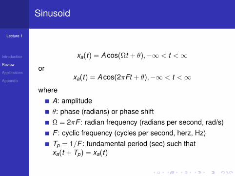
Sinusoid
xa(t) = A cos(Ωt + θ),−∞ < t <∞
orxa(t) = A cos(2πFt + θ),−∞ < t <∞
whereA: amplitudeθ: phase (radians) or phase shiftΩ = 2πF : radian frequency (radians per second, rad/s)F : cyclic frequency (cycles per second, herz, Hz)Tp = 1/F : fundamental period (sec) such thatxa(t + Tp) = xa(t)
Lecture 1
Introduction
Review
Applications
Appendix
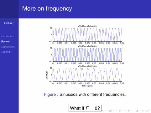
More on frequency
0 0.005 0.01 0.015 0.02 0.025 0.03 0.035 0.04 0.045 0.05−10
0
10x(t)=10cos(2pi(440)t)
0 0.005 0.01 0.015 0.02 0.025 0.03 0.035 0.04 0.045 0.05−10
0
10x(t)=10cos(2pi(880)t)
0 0.005 0.01 0.015 0.02 0.025 0.03 0.035 0.04 0.045 0.05−10
0
10x(t)=10cos(2pi(236)t)
Time t (sec)
Am
plitu
de
Figure : Sinusoids with different frequencies.
What if F = 0?
Lecture 1
Introduction
Review
Applications
Appendix
More on frequency - How does it sound?1
A440A880C236A tuning fork demo
1The multimedia materials are from McClellan, Schafer and Yoder,DSP FIRST: A Multimedia Approach. Prentice Hall, Upper Saddle River,New Jersey, 1998. Copyright (c) 1998 Prentice Hall.
Lecture 1
Introduction
Review
Applications
Appendix
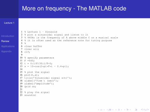
More on frequency - The MATLAB code
1 % Lecture 1 - Sinusoid2 % plot a sinusoidal signal and listen to it3 % 440Hz is the frequency of A above middle C on a musical scale4 % it is often used as the reference note for tuning purpose5 %6 clear buffer7 clear all;8 clf;9
10 % specify parameters11 F =440;12 t = 0:1/F/30:1/F*5;13 x = 10*cos(2*pi*F*t - 0.4*pi);1415 % plot the signal16 plot(t,x);17 title(’Sinusoidal signal x(t)’);18 xlabel(’Time t (sec)’);19 ylabel(’Amplitude’);20 grid on;2122 % play the signal23 sound(x)
Lecture 1
Introduction
Review
Applications
Appendix
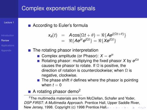
Complex exponential signals
According to Euler’s formula
xa(t) = A cos(Ωt + θ) = <Aej(Ωt+θ)= <AejθejΩt = <XejΩt
The rotating phasor interpretationComplex amplitude (or Phasor): X = ejθ
Rotating phasor: multiplying the fixed phasor X by ejΩt
causes the phasor to rotate. If Ω is positive, thedirection of rotation is counterclockwise; when Ω isnegative, clockwise.The phase shift θ defines where the phasor is pointingwhen t = 0
A rotating phasor demo2
2The multimedia materials are from McClellan, Schafer and Yoder,DSP FIRST: A Multimedia Approach. Prentice Hall, Upper Saddle River,New Jersey, 1998. Copyright (c) 1998 Prentice Hall.
Lecture 1
Introduction
Review
Applications
Appendix
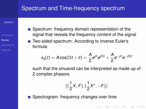
Spectrum and Time-frequency spectrum
Spectrum: frequency domain representation of thesignal that reveals the frequency content of the signalTwo-sided spectrum: According to inverse Euler’sformula
xa(t) = A cos(Ωt + θ) =A2
ejθejΩt +A2
e−jθe−jΩt
such that the sinusoid can be interpreted as made up of2 complex phasors
(12
X ,F ), (12
X ∗,−F )
Spectrogram: frequency changes over time
Lecture 1
Introduction
Review
Applications
Appendix
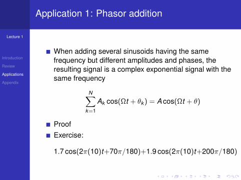
Application 1: Phasor addition
When adding several sinusoids having the samefrequency but different amplitudes and phases, theresulting signal is a complex exponential signal with thesame frequency
N∑k=1
Ak cos(Ωt + θk ) = A cos(Ωt + θ)
ProofExercise:
1.7 cos(2π(10)t+70π/180)+1.9 cos(2π(10)t+200π/180)
Lecture 1
Introduction
Review
Applications
Appendix
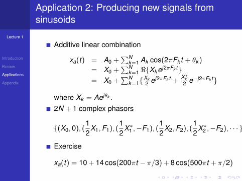
Application 2: Producing new signals fromsinusoids
Additive linear combination
xa(t) = A0 +∑N
k=1 Ak cos(2πFk t + θk )
= X0 +∑N
k=1<Xkej2πFk t= X0 +
∑Nk=1
Xk2 ej2πFk t +
X∗k
2 e−j2πFk t
where Xk = Aejθk .2N + 1 complex phasors
(X0,0), (12
X1,F1), (12
X ∗1 ,−F1), (
12
X2,F2), (12
X ∗2 ,−F2), · · ·
Exercise
xa(t) = 10 + 14 cos(200πt − π/3) + 8 cos(500πt + π/2)
Lecture 1
Introduction
Review
Applications
Appendix
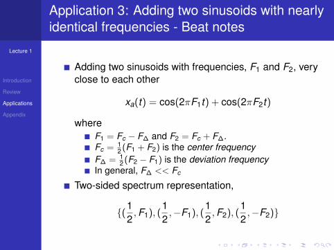
Application 3: Adding two sinusoids with nearlyidentical frequencies - Beat notes
Adding two sinusoids with frequencies, F1 and F2, veryclose to each other
xa(t) = cos(2πF1t) + cos(2πF2t)
whereF1 = Fc − F∆ and F2 = Fc + F∆.Fc = 1
2 (F1 + F2) is the center frequencyF∆ = 1
2 (F2 − F1) is the deviation frequencyIn general, F∆ << Fc
Two-sided spectrum representation,
(12,F1), (
12,−F1), (
12,F2), (
12,−F2)
Lecture 1
Introduction
Review
Applications
Appendix
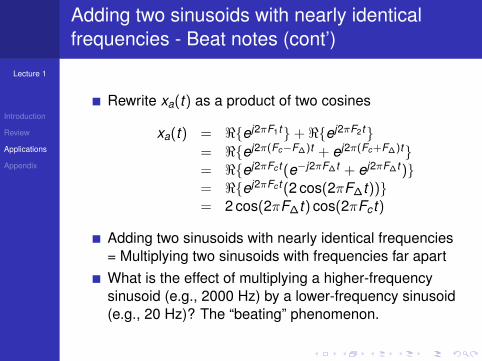
Adding two sinusoids with nearly identicalfrequencies - Beat notes (cont’)
Rewrite xa(t) as a product of two cosines
xa(t) = <ej2πF1t+ <ej2πF2t= <ej2π(Fc−F∆)t + ej2π(Fc+F∆)t= <ej2πFc t (e−j2πF∆t + ej2πF∆t )= <ej2πFc t (2 cos(2πF∆t))= 2 cos(2πF∆t) cos(2πFc t)
Adding two sinusoids with nearly identical frequencies= Multiplying two sinusoids with frequencies far apartWhat is the effect of multiplying a higher-frequencysinusoid (e.g., 2000 Hz) by a lower-frequency sinusoid(e.g., 20 Hz)? The “beating” phenomenon.
Lecture 1
Introduction
Review
Applications
Appendix
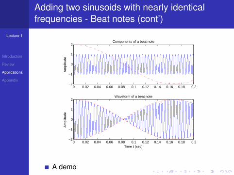
Adding two sinusoids with nearly identicalfrequencies - Beat notes (cont’)
0 0.02 0.04 0.06 0.08 0.1 0.12 0.14 0.16 0.18 0.2−2
−1
0
1
2Components of a beat note
Am
plitu
de
0 0.02 0.04 0.06 0.08 0.1 0.12 0.14 0.16 0.18 0.2−2
−1
0
1
2Waveform of a beat note
Time t (sec)
Am
plitu
de
A demo
Lecture 1
Introduction
Review
Applications
Appendix
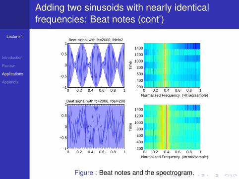
Adding two sinusoids with nearly identicalfrequencies: Beat notes (cont’)
0 0.2 0.4 0.6 0.8 1−1
−0.5
0
0.5
1Beat signal with fc=2000, fdel=2
0 0.2 0.4 0.6 0.8 1200
400
600
800
1000
1200
1400
Normalized Frequency (×π rad/sample)
Tim
e
0 0.2 0.4 0.6 0.8 1−1
−0.5
0
0.5
1Beat signal with fc=2000, fdel=200
0 0.2 0.4 0.6 0.8 1200
400
600
800
1000
1200
1400
Normalized Frequency (×π rad/sample)
Tim
e
Figure : Beat notes and the spectrogram.
Lecture 1
Introduction
Review
Applications
Appendix
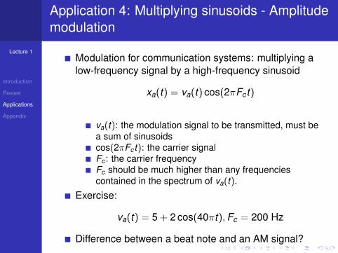
Application 4: Multiplying sinusoids - Amplitudemodulation
Modulation for communication systems: multiplying alow-frequency signal by a high-frequency sinusoid
xa(t) = va(t) cos(2πFc t)
va(t): the modulation signal to be transmitted, must bea sum of sinusoidscos(2πFc t): the carrier signalFc : the carrier frequencyFc should be much higher than any frequenciescontained in the spectrum of va(t).
Exercise:
va(t) = 5 + 2 cos(40πt),Fc = 200 Hz
Difference between a beat note and an AM signal?

Lecture 1
Introduction
Review
Applications
Appendix
Multiplying sinusoids - Amplitude modulation(cont’)
0 0.02 0.04 0.06 0.08 0.1 0.12 0.14 0.16 0.18 0.2−8
−6
−4
−2
0
2
4
6
8Waveform of the AM signal
Time t (sec)
Am
plitu
de
A demo
Lecture 1
Introduction
Review
Applications
Appendix
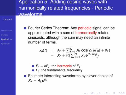
Application 5: Adding cosine waves withharmonically related frequencies - Periodicwaveforms
Fourier Series Theorem: Any periodic signal can beapproximated with a sum of harmonically relatedsinusoids, although the sum may need an infinitenumber of terms.
xa(t) = A0 +∑N
k=1 Ak cos(2πkF0t + θk )
= X0 + <∑N
k=1 Xkej2πkF0t
Fk = kF0: the harmonic of F0F0: the fundamental frequency
Estimate interesting waveforms by clever choice ofXk = Akejθk
Lecture 1
Introduction
Review
Applications
Appendix
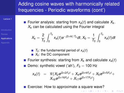
Adding cosine waves with harmonically relatedfrequencies - Periodic waveforms (cont’)
Fourier analysis: starting from xa(t) and calculate Xk .Xk can be calculated using the Fourier integral
Xk =2T0
∫ T0
0xa(t)e−j2πkt/T0dt ,X0 =
1T0
∫ T0
0xa(t)dt
T0: the fundamental period of xa(t)X0: the DC component
Fourier synthesis: starting from Xk and calculate xa(t)Demo: synthetic vowel (’ah’), F0 = 100 Hz
xa(t) = <X2ej2π2F0t + X4ej2π4F0t + X5ej2π5F0t +X16ej2π16F0t + X17ej2π17F0t
Exercise: How to approximate a square wave?
Lecture 1
Introduction
Review
Applications
Appendix
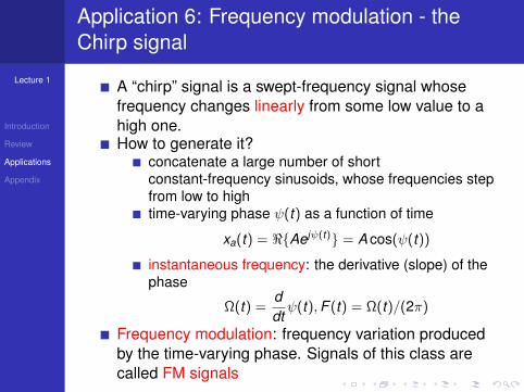
Application 6: Frequency modulation - theChirp signal
A “chirp” signal is a swept-frequency signal whosefrequency changes linearly from some low value to ahigh one.How to generate it?
concatenate a large number of shortconstant-frequency sinusoids, whose frequencies stepfrom low to hightime-varying phase ψ(t) as a function of time
xa(t) = <Aejψ(t) = A cos(ψ(t))
instantaneous frequency: the derivative (slope) of thephase
Ω(t) =ddtψ(t),F (t) = Ω(t)/(2π)
Frequency modulation: frequency variation producedby the time-varying phase. Signals of this class arecalled FM signals
Lecture 1
Introduction
Review
Applications
Appendix
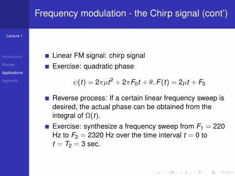
Frequency modulation - the Chirp signal (cont’)
Linear FM signal: chirp signalExercise: quadratic phase
ψ(t) = 2πµt2 + 2πF0t + θ,F (t) = 2µt + F0
Reverse process: If a certain linear frequency sweep isdesired, the actual phase can be obtained from theintegral of Ω(t).Exercise: synthesize a frequency sweep from F1 = 220Hz to F2 = 2320 Hz over the time interval t = 0 tot = T2 = 3 sec.
Lecture 1
Introduction
Review
Applications
Appendix
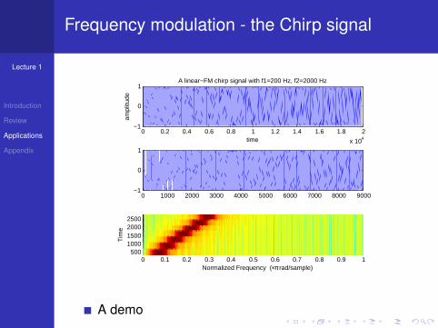
Frequency modulation - the Chirp signal
0 0.2 0.4 0.6 0.8 1 1.2 1.4 1.6 1.8 2
x 104
−1
0
1
time
ampl
itude
A linear−FM chirp signal with f1=200 Hz, f2=2000 Hz
0 1000 2000 3000 4000 5000 6000 7000 8000 9000−1
0
1
0 0.1 0.2 0.3 0.4 0.5 0.6 0.7 0.8 0.9 1500
1000150020002500
Normalized Frequency (×π rad/sample)
Tim
e
A demo
Lecture 1
Introduction
Review
Applications
Appendix
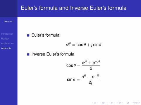
Euler’s formula and Inverse Euler’s formula
Euler’s formula
ejθ = cos θ + j sin θ
Inverse Euler’s formula
cos θ =ejθ + e−jθ
2
sin θ =ejθ − e−jθ
2j
Lecture 1
Introduction
Review
Applications
Appendix
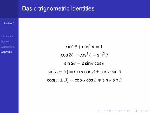
Basic trignometric identities
sin2 θ + cos2 θ = 1
cos 2θ = cos2 θ − sin2 θ
sin 2θ = 2 sin θ cos θ
sin(α± β) = sinα cosβ ± cosα sinβ
cos(α± β) = cosα cosβ ∓ sinα sinβ
Lecture 1
Introduction
Review
Applications
Appendix
Basic properties of the sine and cosinefunctions
Equivalence
sin θ = cos(θ − π/2) or cos θ = sin(θ + π/2)
Periodicity
cos(θ + 2kπ) = cos θ, when k is an integer
Evenness of cosine
cos(−θ) = cos θ
Oddness of sine
sin(−θ) = − sin θ
Lecture 1
Introduction
Review
Applications
Appendix
Basic properties of the sine and cosinefunctions (cont’)
Zeros of sine
sin(πk) = 0, when k is an integer
Ones of cosine
cos(2πk) = 1, when k is an integer
Minus ones of cosine
cos[2π(k +12
)] = −1, when k is an integer
Derivatives
d sin θdθ
= cos θ,d cos θ
dθ= − sin θ