Digital recording and numerical reconstruction of holograms

This article has been downloaded from IOPscience. Please scroll down to see the full text article.

2002 Meas. Sci. Technol. 13 R85

(http://iopscience.iop.org/0957-0233/13/9/201)

Download details:

IP Address: 128.54.47.91

The article was downloaded on 21/07/2010 at 04:54

Please note that terms and conditions apply.

View the table of contents for this issue, or go to the journal homepage for more

Home Search Collections Journals About Contact us My IOPscience

INSTITUTE OF PHYSICS PUBLISHING MEASUREMENT SCIENCE AND TECHNOLOGY

Meas. Sci. Technol. 13 (2002) R85–R101 PII: S0957-0233(02)37262-X

REVIEW ARTICLE

Digital recording and numericalreconstruction of hologramsUlf Schnars1,3 and Werner P O Juptner2

1 Im Grund 7, D-27628 Hagen, Germany2 Bremer Institut fur Angewandte Strahltechnik (BIAS), Klagenfurter Straße 2, D-28359Bremen, Germany

E-mail: schnars@t-online.de

Received 22 May 2002, accepted for publication 17 July 2002Published 7 August 2002Online at stacks.iop.org/MST/13/R85

AbstractThis article describes the principles and major applications of digitalrecording and numerical reconstruction of holograms (digital holography).

Digital holography became feasible since charged coupled devices(CCDs) with suitable numbers and sizes of pixels and computers withsufficient speed became available. The Fresnel or Fourier holograms arerecorded directly by the CCD and stored digitally. No film materialinvolving wet-chemical or other processing is necessary. The reconstructionof the wavefield, which is done optically by illumination of a hologram, isperformed by numerical methods. The numerical reconstruction process isbased on the Fresnel–Kirchhoff integral, which describes the diffraction ofthe reconstructing wave at the micro-structure of the hologram.

In the numerical reconstruction process not only the intensity, but alsothe phase distribution of the stored wavefield can be computed from thedigital hologram. This offers new possibilities for a variety of applications.Digital holography is applied to measure shape and surface deformation ofopaque bodies and refractive index fields within transparent media. Furtherapplications are imaging and microscopy, where it is advantageous torefocus the area under investigation by numerical methods.

Keywords: digital holography, holographic interferometry

1. Introduction

Dennis Gabor [1–3] invented holography in 1948 as a methodfor recording and reconstructing the amplitude and phase of awavefield. The word holography is derived from the Greekwords ‘holos’ meaning ‘whole’ or ‘entire’ and ‘graphein’meaning ‘to write’.

A hologram is the photographically or otherwise recordedinterference pattern between a wavefield scattered from theobject and a coherent background, called the reference wave.A hologram is usually recorded on a flat surface, but containsinformation about the entire three-dimensional wavefield.3 U Schnars works for AIRBUS Deutschland GmbH, but contributed to thiswork as a private individual.

This information is coded in the form of bright and darkmicrointerferences, usually not visible for the human eye dueto the high spatial frequencies. The object wave can bereconstructed by illuminating the hologram with the referencewave again. This reconstructed wave is indistinguishable fromthe original object wave. An observer sees a three-dimensionalimage which exhibits all the effects of perspective and depthof focus.

In the original set-up of Gabor the reference waveand object wave are located along the axis normal tothe photographic plate. This leads to a reconstructedimage superimposed by the bright reconstruction wave anda second image, the so-called ‘twin image’. Significantimprovements of this in-line holography were made by Leith

0957-0233/02/090085+17$30.00 © 2002 IOP Publishing Ltd Printed in the UK R85

Review Article

and Upatnieks [4, 5], who introduced an off-axis referencewave. With their set-up the two images and the reconstructionwave are spatially separated.

One major application of holography is holographicinterferometry (HI), developed in the late 1960s by Stetson andPowell [6, 7] and others. With HI it became possible to map thedisplacements of rough surfaces with an accuracy of a fractionof a micrometre. It is also possible to make interferometriccomparisons of stored wavefronts that exist at different times.

The development of computer technology made it possibleto transfer either the recording process or the reconstructionprocess into the computer. The first approach led to computergenerated holography (CGH), which allows us to generateartificial holograms by numerical methods. These computergenerated holograms are then optically reconstructed. Thistechnique is not considered here: we refer the interested readerto the literature, see, for example, [8–10].

Numerical hologram reconstruction was initiated byYaroslavskii et al [11–13] at the early 1970s. Theysampled optically enlarged parts of in-line and Fourierholograms recorded on a photographic plate. These digitized‘conventional’ holograms were reconstructed numerically.Onural and Scott [14–16] improved the reconstructionalgorithm and applied this method to particle measurement.Haddad et al [73] described a holographic microscope basedon numerical reconstruction of Fourier holograms.

A big step forward was the development of directrecording of Fresnel holograms with charged coupled devices(CCDs) by Schnars and Juptner [17, 18]. This method nowenables full digital recording and processing of holograms,without any photographic recording as an intermediate step.Within the scope of this article digital sampling and numericalhologram reconstruction is called digital holography.

Schnars and Juptner applied their method to interferome-try and demonstrated that digital hologram reconstruction of-fers much more possibilities than conventional (optical) pro-cessing. The phases of the stored light waves can be calcu-lated directly from the digital holograms, without generatingphase-shifted interferograms [19, 20]. Other methods of opti-cal metrology, such as shearography or speckle photography,can be derived numerically from digital holograms [21]. Thismeans that one can choose the interferometric technique (holo-gram interferometry, shearography or other technique) afterhologram recording by mathematical methods.

The use of electronics devices, such as CCDs, forthe recording of interferograms was already established inelectronic speckle pattern interferometry (ESPI, also calledTV holography), discovered independently from each otherby Butters and Leendertz [22], Macovski et al [23] andSchwomma [24]. In this method two speckle interferogramsare recorded at different states of the object under investigation.The speckle patterns are subtracted electronically. Theresulting fringe pattern has some similarities to that ofconventional or digital HI, but the main differences are thespeckle appearance of the fringes and the loss of phase inthe correlation process. The interference phase has to berecovered with phase-shifting methods [26–28], requiringadditional experimental effort (phase-shifting unit). DigitalHI and ESPI are competing methods: the image subtractionin ESPI is simpler than the numerical reconstruction of digital

Figure 1. Hologram recording.

holography, but the information content of digital holograms ishigher. ESPI is not considered here: we refer to correspondingarticles [25, 29, 30].

Since the mid-1990s digital holography has beenmodified, improved and applied to several measurementtasks [31–97].

Important steps are:

• improvements in the experimental techniques andreconstruction algorithm [31–50],

• applications in deformation analysis and shape measure-ment [51–55, 71, 111],

• the development of phase-shifting digital holography [56–64],

• applications in imaging, particle tracking and mi-croscopy [65–70, 73, 104],

• measurement of refractive index distributions withintransparent media [72, 74, 75],

• applications in encrypting information [76, 77],• the development of digital light-in-flight holography [78–

83],• the development of comparative digital holography [84].

Recently it has been demonstrated how to reconstruct digitalholograms optically using a liquid crystal device (LCD) [84]or a digital micromirror device (DMD) [98].

2. Foundations of holography

2.1. Hologram recording and reconstruction

The general set-up for recording off-axis holograms is shownin figure 1 [99, 100]. Light with sufficient coherence length issplit into two partial waves by a beamsplitter (BS). One waveilluminates the object, is scattered and reflected to the recordingmedium, e.g. a photographic plate. The second wave, calledthe reference wave, illuminates the plate directly. Both wavesare interfering. The interference pattern is recorded, e.g. bychemical development of the photographic plate. The recordedinterference pattern is called a hologram.

The original object wave is reconstructed by illuminatingthe hologram with the reference wave, figure 2. An observersees a virtual image, which is indistinguishable from the imageof the original object. The reconstructed image exhibits all theeffects of perspective and depth of focus.

R86

Review Article

Figure 2. Hologram reconstruction.

The holographic process is described mathematically asfollows:

O(x, y) = o(x, y) exp(iϕO (x, y)) (2.1)

is the complex amplitude of the object wave with real amplitudeo and phase ϕO and

R(x, y) = r(x, y) exp(iϕR(x, y)) (2.2)

is the complex amplitude of the reference wave with realamplitude r and phase ϕR .

Both waves interfere at the surface of the recordingmedium. The intensity is calculated by

I (x, y) = |O(x, y) + R(x, y)|2= (O(x, y) + R(x, y))(O(x, y) + R(x, y))∗

= R(x, y)R∗(x, y) + O(x, y)O∗(x, y)

+ O(x, y)R∗(x, y) + R(x, y)O∗(x, y) (2.3)

where * denotes the conjugate complex. The amplitudetransmission h(x, y) of the developed photographic plate (orany other recording media) is proportional to I (x, y):

h(x, y) = h0 + βτ I (x, y) (2.4)

where β is a constant, τ is the exposure time and h0 is theamplitude transmission of the unexposed plate. h(x, y) isalso called the hologram function. In digital holography usingCCDs as recording medium h0 can be neglected.

For hologram reconstruction the amplitude transmissionhas to be multiplied with the complex amplitude of thereconstruction (reference) wave:

R(x, y)h(x, y) = [h0 + βτ(r 2 + o2)]R(x, y)

+ βτr 2 O(x, y) + βτ R2(x, y)O∗(x, y). (2.5)

The first term on the right side of this equation is the referencewave, multiplied by a factor. It represents the undiffractedwave passing through the hologram (zero diffraction order).The second term is the reconstructed object wave, forming thevirtual image. The factor βτr2 only influences the brightnessof the image. The third term produces a distorted real imageof the object. For off-axis holography the virtual image, thereal image and the undiffracted wave are spatially separated.

2.2. Holographic interferometry

HI is an optical method to observe deformations of opaquebodies or refractive index variations in transparent media,e.g. fluids or gases. HI is a non-contact, non-destructivemethod with very high sensitivity. Optical path changes upto one hundredth of a wavelength are resolvable.

Two coherent wavefields, which are reflected from twodifferent states of the object, are interfering. This is achieved,for example, in double-exposure holography by the recordingof two wavefields on a single photographic plate. The firstexposure represents the object in its initial state and the secondexposure represents the object in its loaded (e.g. deformed)state. The hologram is reconstructed by illumination withthe reference wave. As a result of the superposition ofthe two holographic recordings with slightly different objectwaves only one image superimposed by interference fringesis reconstructed. From this holographic interferogram theobserver can determine optical path changes due to the objectdeformation or other effects.

In the real time technique the hologram is replaced,after processing, in exactly the same position in which itwas recorded. When it is illuminated with the referencewave, the reconstructed virtual image coincides with theobject. Interference patterns due to phase changes betweenthe holographically reconstructed initial object wave and theactual object wave are observable in real time.

The following mathematical description is valid for thedouble exposure and real time techniques. The complexamplitude of the object wave in the initial state is

O1(x, y) = o(x, y) exp[iϕ(x, y)] (2.6)

where o(x, y) is the real amplitude and ϕ(x, y) is the phase ofthe object wave.

Optical path changes due to deformations of the objectsurface can be described by a variation of the phase fromϕ to ϕ + �ϕ. �ϕ is the difference between the initial andactual phase, and is called the interference phase. The complexamplitude of the actual object wave is therefore denoted by

O2(x, y) = o(x, y) exp[i(ϕ(x, y) + �ϕ(x, y))]. (2.7)

The intensity of a holographic interference pattern isdescribed by the square of the sum of the complex amplitudes.It is calculated as follows:

I (x, y) = |O1 + O2|2 = (O1 + O2)(O1 + O2)∗

= 2o2(1 + cos(�ϕ)). (2.8)

Equation (2.8) describes the relation between the intensityof the interference pattern and the interference phase, whichcontains the information about the deformation.

It is not possible to calculate the interference phasedistribution correctly from one single fringe pattern, becausethe cosine is an even function (cos 30◦ = cos −30◦) and thesign of the argument is not determined unequivocally. In mostpractical cases distortions have to be considered in addition.The interference pattern is superimposed by speckle noiseand the brightness of the pattern varies due to the profile ofthe illuminating laser beam. Therefore several techniqueshave been developed to determine the interference phase by

R87

Review Article

Figure 3. Definition of the sensitivity vector.

recording additional information. The most commonly usedtechniques are the various phase-shifting methods [100–102].Three or more interferograms are reconstructed with mutualphase shifts. The interference phase is calculated from thesephase-shifted intensity distributions.

The interference phase is the key to calculate quantitiesrepresenting the object under investigation. These are thedisplacement vector field of the surface in the case of opaquebodies or refractive index changes within transparent media.A third application of HI is to measure the shape of bodies(contouring). In the following we describe the applicationof HI to measure surface displacements. For a detaileddescription of the other applications we refer to the literature,see, for example, [100].

The relation between the measured interference phase andthe displacement vector field �d(x, y, z) of the object surfaceunder investigation is given by the following equation [100, p72], [103]:

�ϕ(x, y) = 2π

λ�d(x, y, z)(�b − �s) = 2π

λ�d(x, y, z)�S (2.9)

where �b and �s are unit vectors in the illumination andobservation directions, see figure 3. The vector �S is calledthe sensitivity vector. The sensitivity vector is defined onlyby the geometry of the holographic arrangement. It givesthe direction in which the set-up has maximum sensitivity.At each point we measure the projection of the displacementvector onto the sensitivity vector. Equation (2.9) is the basisof all quantitative measurements of the deformation of opaquebodies.

In the general case of a three-dimensional deformationfield equation (2.9) contains the three components of �d asunknown parameters. In this case three interferograms of thesame surface with linear independent sensitivity vectors arenecessary to determine the displacement. In many practicalcases it is not the three-dimensional displacement field, but thedeformation perpendicular to the surface, which is of interest.In this case an optimized set-up with parallel illumination andobservation direction is used (�S = (0, 0, 2)). The componentdz is then calculated from the interference phase by

dz = �ϕλ

4π. (2.10)

A phase variation of 2π corresponds to a deformation of λ/2.

Figure 4. Digital holography: (a) recording, (b) reconstruction.

3. Digital holography

3.1. General principles

A general set-up for digital recording of off-axis hologramsis shown in figure 4 [18]. A plane reference wave and thewave reflected from the object are interfering at the surfaceof a CCD. The resulting hologram is electronically recordedand stored. The object is, in general, a three-dimensional bodywith diffusely reflecting surface, located at a distance d fromthe CCD.

In optical reconstruction the virtual image appears at theposition of the original object and the real image is formed alsoat a distance d, but in the opposite direction from the CCD, seefigure 4(b).

The diffraction of a light wave at an aperture (in this casea hologram) which is fastened perpendicular to the incomingbeam is described by the Fresnel–Kirchhoff integral [105, p266]:

�(ξ, η) = i

λ

∫ ∞

−∞

∫ ∞

−∞h(x, y)R(x, y)

exp(−i 2π

λρ)

ρ

× (12 + 1

2 cos θ)

dx dy (3.1)

withρ =

√(x − ξ)2 + (y − η)2 + d2 (3.2)

where h(x, y) is again the hologram function and ρ is thedistance between a point in the hologram plane and a pointin the reconstruction plane, see figure 5. The angle θ is alsodefined in figure 5. For a plane reference wave R(x, y) issimply given by the real amplitude:

R = r + i0 = r. (3.3)

The diffraction pattern is calculated at a distance d behindthe CCD plane, which means it reconstructs the complexamplitude in the plane of the real image.

Equation (3.1) is the basis for numerical hologramreconstruction. Because the reconstructed wavefield �(ξ, η)

is a complex function, both the intensity as well as the phasecan be calculated [19]. This is in contrast to the case of optical

R88

Review Article

Figure 5. Coordinate system.

hologram reconstruction, in which only the intensity is madevisible. This interesting property of digital holography is usedin digital HI, see section 4.

There are a few slightly different formulae of the Fresnel–Kirchhoff integral in the literature, which differ, for example,by the sign of the argument of the exponential function(exp(+i . . .) instead of exp(−i . . .)). However, with the ‘+’sign as well the same expressions result for the intensity andmagnitude of the interference phase used in digital HI.

The set-up of figure 4 is often used in digital holography,because a plane wave propagating perpendicularly to thesurface of the CCD can be easily arranged in the laboratory.Another advantage is that for this geometry the reconstructedreal image has no geometrical distortions (this can be derivedfrom the holographic imaging equations, see, for example,[100, pp 45–8]). Other recording geometries are discussedin section 3.6.

3.2. Reconstruction by the Fresnel transformation

3.2.1. Fresnel approximation. For x and y values as well asfor ξ and η values which are small compared to the distance dbetween the reconstruction plane and the CCD expression (3.2)can be replaced by the first terms of the Taylor series:

ρ = d +(ξ − x)2

2d+

(η − x)2

2d− 1

8

[(ξ − x)2 + (η − x)2]

d3+ · · ·

≈ d +(ξ − x)2

2d+

(η − y)2

2d(3.4)

with the additional approximation cos θ ≈ 1, and by replacingthe dominator in (3.1) by d the following expression results:

�(ξ, η) = i

λdexp

(−i

2π

λd

) ∫ ∞

−∞

∫ ∞

−∞R(x, y)h(x, y)

× exp

[−i

π

λd((ξ − x)2 + (η − y)2)

]dx dy. (3.5)

If we carry out the multiplications in the argument of theexponential under the integral we get

�(ξ, η) = i

λdexp

(−i

2π

λd

)exp

[−i

π

λd(ξ 2 + η2)

]

×∫ ∞

−∞

∫ ∞

−∞R(x, y)h(x, y) exp

[−i

π

λd(x2 + y2)

]

× exp

[i2π

λd(xξ + yη)

]dx dy. (3.6)

Figure 6. Reconstruction of the virtual image.

This equation is called the Fresnel approximation or Fresneltransformation. It enables reconstruction of the wavefield in aplane behind the hologram, in this case in the plane of the realimage. The intensity is calculated by squaring

I (ξ, η) = |�(ξ, η)|2. (3.7)

The phase is calculated by

ϕ(ξ, η) = arctanIm[�(ξ, η)]

Re[�(ξ, η)](3.8)

where Re denotes the real part and Im the imaginary part.Reconstruction of the virtual image is also possible by

introducing the imaging properties of a lens into the numericalreconstruction process [20, pp 35–6]. This lens correspondsto the eye lens of an observer watching through an opticallyreconstructed hologram. In the simplest case this lens islocated directly behind the hologram, figure 6. The imagingproperties of a lens with focal distance f are considered by acomplex factor [99, p 259]

L(x, y) = exp

[iπ

λ f(x2 + y2)

]. (3.9)

For a magnification of 1 a focal distance of f = d/2 hasto be used. The complex amplitude in the image plane is thencalculated by

�(ξ, η) = i

λdexp

(−i

2π

λd

)exp[−i

π

λd(ξ 2 + η2)]

×∫ ∞

−∞

∫ ∞

−∞R(x, y)L(x, y)h(x, y) exp

[−i

π

λd(x2 + y2)

]

× exp

[i2π

λd(xξ + yη)

]dx dy

R89

Review Article

= i

λdexp

(−i

2π

λd

)exp

[−i

π

λd(ξ 2 + η2)

]

×∫ ∞

−∞

∫ ∞

−∞R(x, y)h(x, y) exp

[+i

π

λd(x2 + y2)

]

× exp

[i2π

λd(xξ + yη)

]dx dy. (3.10)

Compared with (3.6) only the sign of the argument of the firstexponential function in the integral changes.

3.2.2. Discrete Fresnel transformation. For digitizationof the Fresnel transform (3.6) we introduce the followingsubstitutions [13]:

ν = ξ

λd; µ = η

λd. (3.11)

Herewith (3.6) becomes

�(ν,µ) = i

λdexp[−iπλd(ν2 + µ2)]

×∫ ∞

−∞

∫ ∞

−∞R(x, y)h(x, y) exp

[−i

π

λd(x2 + y2)

]× exp[i2π(xν + yµ)] dx dy. (3.12)

The factor exp(−i2π/λd) is omitted, since it only affectsthe overall phase. It has no effect on the intensity andinterference phase of digital HI.

A comparison of (3.12) with the definition of the two-dimensional Fourier transform shows that the Fresnel approx-imation is, up to a spherical phase factor, the inverse Fouriertransformation of R(x, y)h(x, y) exp[−iπ/λd(x2 + y2)]:

�(ν,µ) = i

λdexp[−iπλd(ν2 + µ2)]

× �−1

{R(x, y)h(x, y) exp

[−i

π

λd(x2 + y2)

]}. (3.13)

The function � can be digitized if the hologram functionh(x, y) is sampled on a rectangular raster of N × N points,with steps �x and �y along the coordinates. �x and �y arethe distances between neighbouring pixels on the CCD in thehorizontal and vertical directions. With these discrete valuesthe integrals of (3.12) are converted to finite sums:

�(m, n) = i

λdexp[−iπλd(m2�ν2 + n2�µ2)]

×N−1∑k=0

N−1∑l=0

R(k, l)h(k, l) exp

[−i

π

λd(k2�x2 + l2�y2)

]× exp[i2π(k�xm�ν + l�yn�µ)] (3.14)

for m = 0, 1, . . . , N − 1; n = 0, 1, . . . , N − 1.According to the theory of Fourier transform among �x ,

�y and �ν, �µ the following relation exists [106]:

�ν = 1

N�x; �µ = 1

N�y. (3.15)

After re-substitution:

�ξ = λd

N�x; �η = λd

N�y. (3.16)

Figure 7. Digital hologram.

With the use of these equations (3.14) converts to

�(m, n) = i

λdexp

[−iπλd

(m2

N 2�x2+

n2

N 2�y2

)]

×N−1∑k=0

N−1∑l=0

R(k, l)h(k, l) exp

[−i

π

λd(k2�x2 + l2�y2)

]

× exp

[i2π

(km

N+

ln

N

)]. (3.17)

This is the discrete Fresnel transform. The matrix� is calculated by multiplying R(k, l) with h(k, l) andexp[−iπ/(λd)(k2�x2 + l2�y2)] and applying an inversediscrete Fourier transform to the product. The calculation isdone most effectively using the fast Fourier transform (FFT)algorithm. The factor in front of the sum is only affecting thephase and can be neglected for most applications.

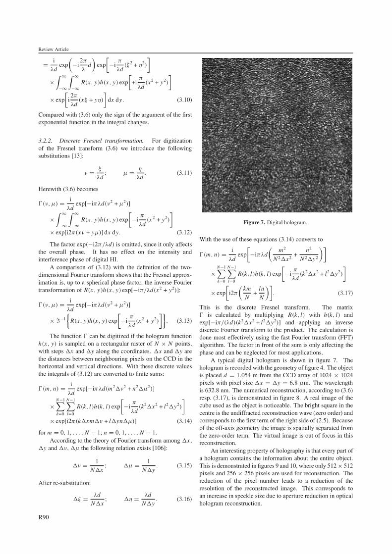
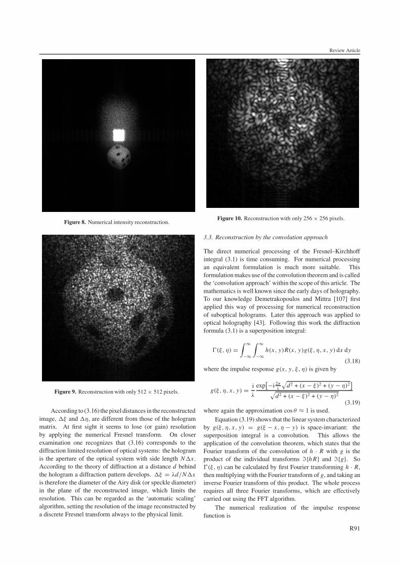
A typical digital hologram is shown in figure 7. Thehologram is recorded with the geometry of figure 4. The objectis placed d = 1.054 m from the CCD array of 1024 × 1024pixels with pixel size �x = �y = 6.8 µm. The wavelengthis 632.8 nm. The numerical reconstruction, according to (3.6)resp. (3.17), is demonstrated in figure 8. A real image of thecube used as the object is noticeable. The bright square in thecentre is the undiffracted reconstruction wave (zero order) andcorresponds to the first term of the right side of (2.5). Becauseof the off-axis geometry the image is spatially separated fromthe zero-order term. The virtual image is out of focus in thisreconstruction.

An interesting property of holography is that every part ofa hologram contains the information about the entire object.This is demonstrated in figures 9 and 10, where only 512 × 512pixels and 256 × 256 pixels are used for reconstruction. Thereduction of the pixel number leads to a reduction of theresolution of the reconstructed image. This corresponds toan increase in speckle size due to aperture reduction in opticalhologram reconstruction.

R90

Review Article

Figure 8. Numerical intensity reconstruction.

Figure 9. Reconstruction with only 512 × 512 pixels.

According to (3.16) the pixel distances in the reconstructedimage, �ξ and �η, are different from those of the hologrammatrix. At first sight it seems to lose (or gain) resolutionby applying the numerical Fresnel transform. On closerexamination one recognizes that (3.16) corresponds to thediffraction limited resolution of optical systems: the hologramis the aperture of the optical system with side length N�x .According to the theory of diffraction at a distance d behindthe hologram a diffraction pattern develops. �ξ = λd/N�xis therefore the diameter of the Airy disk (or speckle diameter)in the plane of the reconstructed image, which limits theresolution. This can be regarded as the ‘automatic scaling’algorithm, setting the resolution of the image reconstructed bya discrete Fresnel transform always to the physical limit.

Figure 10. Reconstruction with only 256 × 256 pixels.

3.3. Reconstruction by the convolution approach

The direct numerical processing of the Fresnel–Kirchhoffintegral (3.1) is time consuming. For numerical processingan equivalent formulation is much more suitable. Thisformulation makes use of the convolution theorem and is calledthe ‘convolution approach’ within the scope of this article. Themathematics is well known since the early days of holography.To our knowledge Demetrakopoulos and Mittra [107] firstapplied this way of processing for numerical reconstructionof suboptical holograms. Later this approach was applied tooptical holography [43]. Following this work the diffractionformula (3.1) is a superposition integral:

�(ξ, η) =∫ ∞

−∞

∫ ∞

−∞h(x, y)R(x, y)g(ξ, η, x, y) dx dy

(3.18)where the impulse response g(x, y, ξ, η) is given by

g(ξ, η, x, y) = i

λ

exp[−i 2π

λ

√d2 + (x − ξ)2 + (y − η)2

]√

d2 + (x − ξ)2 + (y − η)2

(3.19)where again the approximation cos θ ≈ 1 is used.

Equation (3.19) shows that the linear system characterizedby g(ξ, η, x, y) = g(ξ − x, η − y) is space-invariant: thesuperposition integral is a convolution. This allows theapplication of the convolution theorem, which states that theFourier transform of the convolution of h · R with g is theproduct of the individual transforms �{h R} and �{g}. So�(ξ, η) can be calculated by first Fourier transforming h · R,then multiplying with the Fourier transform of g, and taking aninverse Fourier transform of this product. The whole processrequires all three Fourier transforms, which are effectivelycarried out using the FFT algorithm.

The numerical realization of the impulse responsefunction is

R91

Review Article

g(k, l) = i

λ

exp[−i 2π

λ

√d2 +

(k − N

2

)2�x2 +

(l − N

2

)2�y2

]√

d2 +(k − N

2

)2�x2 +

(l − N

2

)2�y2

.

(3.20)The shift of the coordinates by N/2 is on symmetry reasons.

In short notation the reconstruction into the real imageplane is

�(ξ, η) = �−1{�(h · R) · �(g)}. (3.21)

The Fourier transform of g(k, l) can be calculated andexpressed analytically:

G(n, m)

= exp

−i

2πd

λ

√1 − λ2

(n + N 2�x2

2dλ

)2

N 2�x2− λ2

(m + N 2�y2

2dλ

)2

N 2�y2

.

(3.22)

This saves one Fourier transform for reconstruction:

�(ξ, η) = �−1{�(h · R) · G}. (3.23)

For the reconstruction of the virtual image a lenstransmission factor according to (3.9) has to be considered:

�(ξ, η) = �−1{�(h · R · L) · G}. (3.24)

The convolution approach can be applied also to theFresnel approximation [43].

The pixel sizes of the images reconstructed by theconvolution approach are equal to that of the hologram:

�ξ = �x; �η = �y. (3.25)

The pixel sizes of the reconstruction are thereforedifferent from those of the Fresnel approximation (3.16).Reconstruction of holograms by the convolution approachresult indeed in images with more or less pixels per unit lengththan those reconstructed by the Fresnel transform. However,the image resolution does not change due to the physical limitsdiscussed at the end of section 3.2.2. The convolution approachis advantageously applied to reconstruct in-line hologramsfrom particle distributions within transparent media. In thiscase the scale of the reconstructions should be the same forall reconstruction distances in order to localize particles orbubbles within the object volume.

3.4. Suppression of the DC term

The bright square in the centre of figure 8 is the undiffractedreconstruction wave. This zero-order or DC term disturbs theimage, because it covers all object parts lying behind. Methodshave been developed therefore to suppress this term [44].

To understand the cause of this DC term we considerthe hologram formation according to (2.3). The equationis rewritten by inserting the definitions of R and O andmultiplying the terms:

I (x, y) = r(x, y)2 +o(x, y)2 +2r(x, y)o(x, y) cos(ϕO − ϕR).

(3.26)The first two terms lead to the DC term in the

reconstruction process. The third term is statistically varying

between ±2ro from pixel to pixel in the CCD. The averageintensity of all pixels of the hologram matrix is

Im = 1

N 2

N−1∑k=0

N−1∑l=0

I (k�x, l�y) (3.27)

r 2 + o2 now can be suppressed by subtracting this averageintensity Im from the hologram:

I ′(k�x, l�y) = I (k�x, l�y) − Im(k�x, l�y) (3.28)

for k = 0, . . . , N − 1; l = 0, . . . , N − 1.The reconstruction of I ′ results in an image free of the

zero order.Instead of subtracting the average intensity it is also

possible to filter the hologram matrix by a high-pass with lowcut-off frequency [44].

Another method for suppressing the DC term is to measurethe intensities of the reference wave and object wave separately.However, this requires greater experimental effort due to theadditional measurements required.

3.5. Spatial frequency limitation

The light-sensitive material used to record holograms mustresolve the interference pattern resulting from superpositionof the waves scattered from all object points and the referencewave. The maximum spatial frequency, which has to beresolved, is determined by the maximum angle θmax betweenthese waves [108]:

fmax = 2

λsin

(θmax

2

). (3.29)

Photographic emulsions used in optical holography haveresolutions up to 5000 linepairs per millimetre (Lp mm−1).With these materials, holograms with angles between thereference and the object wave of up to 180◦ can be recorded.However, the distance between neighbouring pixels of a CCDis only of the order of �x ≈ 10 µm. The correspondingmaximum resolvable spatial frequency calculated by

fmax = 1

2�x(3.30)

is therefore of the order of 50 Lp mm−1. According to (3.29)the maximum angle between the reference and object wave istherefore limited to a few degrees. In this case the sine functionin (3.29) can be approximated by the argument

fmax ≈ θmax

λ. (3.31)

3.6. Recording set-ups

Typical set-ups used in digital holography are shown infigure 11. In figure 11(a) a plane reference wave accordingto (3.3) is used, which propagates perpendicularly to the CCD.The object is located unsymmetrical with respect to the centreline. This set-up is very simple, but the space occupied bythe object is not used effectively. In figure 11(b) the planereference wave is coupled into the set-up via a beamsplitter.This allows us to position the object symmetrically. At a given

R92

Review Article

Figure 11. Recording set-ups.

distance d objects with larger dimensions can be recorded.However, the DC term is in the centre of the reconstructedimage and has to be suppressed by the procedure described insection 3.4.

In figure 11(c) the reference wave impinges onto the CCDunder an angle α. The reference wave is described by

R = exp

(−i

2π

λx sin α

). (3.32)

Figure 11(d) is called lensless Fourier holography. It hasbeen realized also in digital holography [39]. The point sourceof the spherical reference wave is located in the plane of theobject:

R = exp(−i 2π

λ

√(d2 + x2 + y2)

)√

(d2 + x2 + y2)

≈ 1

dexp

(−i

2π

λd

)exp

(−i

π

λd(x2 + y2)

). (3.33)

Again the Fresnel approximation is used for the squareroot. Inserting this expression into the reconstruction formulafor the virtual image (3.10) leads to the following equation:

�(ξ, η) = C exp

[−i

π

λd(ξ 2 + η2)

]�−1{h(x, y)} (3.34)

where C is a complex constant. A lensless Fourier hologram istherefore reconstructed by a Fourier transform. The effect ofthe spherical phase factor associated with the Fresnel transformis eliminated by the use of a spherical reference wave with thesame curvature.

If objects with dimensions larger than a few centimetresare be recorded by CCDs, the recording distance d increasesup to several metres. This is not feasible in practice.Therefore set-ups have been developed which reduce theobject angle in order to make the spatial frequency spectrumresolvable [32, 109]. An example of such a set-up is shown infigure 12. A divergent lens is positioned between the object andthe target. This lens generates a reduced virtual image of theobject in a distance d ′. The object wavefield is not recorded,but rather that of the reduced virtual image. The referencewave is superimposed by a beamsplitter.

3.7. Phase-shifting digital holography

The amplitude and phase of a light wave can be reconstructedfrom a single hologram by the methods described in thepreceding sections. A completely different approach has beenproposed by Skarman [56, 57]. He used a phase-shiftingalgorithm to calculate the initial phase and therefore thecomplex amplitude in a certain plane, e.g. the image planeor any other plane. With this initial complex amplitude it ispossible to calculate the wave field in any other plane using theFresnel–Kirchhoff integral. Later this phase-shifting digitalholography was improved and applied to opaque objects byYamaguchi et al [58–60, 62–64].

The principal arrangement for phase-shifting digitalholography is shown in figure 13. The object wave andreference wave are interfering at the surface of a CCD.The reference wave is guided via a mirror mounted on apiezoelectric transducer (PZT). With this PZT the phase ofthe reference wave can be shifted stepwise. The principle ofphase-shifting interferometry is to record several (at least three)interferograms with mutual phase shifts. The object phase ϕO

is then calculated from these phase-shifted interferograms. Wewill not repeat here the various phase-shifting algorithms, butrefer the reader to the literature, see, for example, [100]. Thereal amplitude o(x, y) of the object wave can be measured fromthe intensity by blocking the reference wave.

As a result the complex amplitude

O(x, y) = o(x, y) exp

(+i

2π

λϕO (x, y)

)(3.35)

of the object wave is determined in the recording (x, y) plane.Now we can use the Fresnel–Kirchhoff integral to

calculate the complex amplitude in any other plane. An imageof the object is calculated by introducing an artificial lens withf = d/2 according to (3.9) at the recording plane. With theFresnel approximation the complex amplitude in the imageplane is then calculated by

�(ξ, η) = C exp

[−i

π

λd(ξ 2 + η2)

]

×∫ ∞

−∞

∫ ∞

−∞O(x, y)L(x, y) exp

[−i

π

λd(x2 + y2)

]

× exp

[i2π

λd(xξ + yη)

]dx dy

= C exp

[− iπ

λd(ξ 2 + η2)

] ∫ ∞

−∞

∫ ∞

−∞O(x, y)

× exp

[+i

π

λd(x2 + y2)

]exp

[i2π

λd(xξ + yη)

]dx dy.

(3.36)

R93

Review Article

Figure 12. Recording geometry for large objects.

Figure 13. Phase-shifting digital holography.

The advantage of phase-shifting digital holography isthat the reconstructed image is free from the zero-order termand from the conjugate image. However, the price for thisachievement is the higher technical effort: phase-shiftedinterferograms have to be generated, restricting the methodto slowly varying phenomena with constant phase during therecording cycle.

4. Digital holographic interferometry

4.1. Deformation measurement

In conventional HI two waves, scattered from an object indifferent states, are superimposed. The resulting holographicinterferogram carries information about the phase changebetween the waves in the form of dark and bright fringes.However, as described in section 2.2, the interference phasecannot be extracted unequivocally from a single interferogram.The interference phase is usually calculated from three or morephase-shifted interferograms by a phase-shifting algorithm.This requires additional experimental effort.

In digital holography a completely different way ofprocessing is possible [19]. In each state of the object adigital hologram is recorded. Instead of superimposing theseholograms as in conventional HI using photographic plates, thedigital holograms are reconstructed separately according to thetheory of section 3. From the resulting complex amplitudes�1(ξ, η) and �2(ξ, η) the phases are calculated:

ϕ1(ξ, η) = arctanIm �1(ξ, η)

Re �1(ξ, η)(4.1)

ϕ2(ξ, η) = arctanIm �2(ξ, η)

Re �2(ξ, η). (4.2)

The index 1 denotes the first (undeformed) state and theindex 2 is for the second (deformed) state. In (4.1) and (4.2) thephase takes values between −π and π , the principal values ofthe arctan function. The interference phase is now calculateddirectly by subtraction:

�ϕ ={

ϕ1 − ϕ2 if ϕ1 � ϕ2

ϕ1 − ϕ2 + 2π if ϕ1 < ϕ2.(4.3)

This equation permits the calculation of the interferencephase directly from the digital holograms. The generation andevaluation of an interferogram is not necessary.

An example of digital HI is shown in figure 14. Theupper left and upper right figures show two digital holograms,recorded at different states. Between the two recordings theknight has been tilted by a small amount. Each hologramis reconstructed separately by a numerical Fresnel transform.The reconstructed phases according to (4.1) and (4.2) aredepicted in the two figures of the middle row. The phasesvary randomly due to the surface roughness of the object.Subtraction of the phases according to (4.3) results in theinterference phase, lower left figure.

The interference phase is indefinite to an additive multipleof 2π . The information about the additive constant is alreadylost in the holographic interferometric process. This is not aconsequence of digital HI, but is valid for all interferometricmethods using wavelength as a length unit. To convertthe interference phase modulo 2π into a continual phasedistribution, one can apply the standard phase unwrappingalgorithm developed for conventional HI or ESPI. These phaseunwrapping procedures are therefore not repeated here, insteadwe refer to textbooks (see, for example, [100, pp 161–70]). Theunwrapped phase image of the example is shown in the lowerright picture of figure 14. This plot corresponds to the objectdisplacement, because the sensitivity vector is nearly constantand perpendicular over the whole surface.

An application of digital HI is the measurement oftransient deformations due to impact loading [32, 109],because only one single recording is necessary in eachdeformation state. As an example, we present the transientdeformation field of a plate made of fibre-reinforced material.The dimensions of the plate are 12 cm × 18 cm. Thereforethe optical set-up of figure 14 is used for hologram recording

R94

Review Article

Figure 14. Digital HI (from [110]).

in order to reduce the spatial frequencies. A pneumaticallyaccelerated steel ball hits the plate and causes a transientdeformation. Two holograms are recorded: the first exposuretakes place before the impact, when the plate is at rest.The second hologram is recorded a few microseconds afterthe impact. The holograms are recorded by a pulsed rubylaser with a pulse duration of about 30 ns. The secondhologram recording is triggered by a photoelectric barrier,which generates the start signal for the laser after the ball hascrossed. As a typical result, the interference phase modulo 2π

and the unwrapped phase are shown in figures 15 and 16. Theunwrapped phase corresponds to the deformation field 5 µsafter the impact.

4.2. Shape measurement

HI can produce an image of a three-dimensional objectmodulated by a fringe pattern corresponding to contours ofconstant elevation with respect to a reference plane [99, p 246].The shape of the object is determined by these contour fringesand by the geometry of the recording set-up. Holographiccontour fringes can be generated either by changing therecording wavelength (two-wavelength method), by varyingthe refractive index of the medium of light propagation(two-refractive index method) or by changing the angle ofillumination.

Figure 15. Interference phase modulo 2π .

Figure 16. Unwrapped phase, corresponding to deformation 5 µsafter the impact.

For shape measurement by the two-wavelength methodtwo holograms are recorded with different wavelengths λ1 andλ2. In conventional HI both holograms are recorded on a singlephotographic plate. Both holograms are now reconstructed byone wavelength, e.g. λ1. Therefore two images of the objectare generated. The image recorded and reconstructed by λ1 isan exact duplicate of the original object surface. The imagewhich has been recorded with λ1, but is reconstructed with λ2,is slightly shifted in observation direction with respect to theoriginal surface. These two reconstructed images interfere.For the special case of parallel illumination and observationdirections which do not vary across the surface the followingequation results for the height steps between neighbouringfringes:

�H = λ1λ2

2|λ1 − λ2| = �

2. (4.4)

This equation is valid for small wavelength differences. Theexpression

� = λ1λ2

|λ1 − λ2| (4.5)

is called the synthetic or equivalent wavelength.The concept of two-wavelength contouring has been

introduced also into digital holography [20, pp 59–60],[39, 71]. Two holograms are recorded with λ1 and λ2 and

R95

Review Article

stored electronically. In contrast to conventional HI usingphotographic plates, both holograms can be reconstructedseparately by the correct wavelengths, according to the theoryof section 3. From the resulting complex amplitudes �λ1(ξ, η)

and �λ2(ξ, η) the phases are calculated:

ϕλ1(ξ, η) = arctanIm �λ1(ξ, η)

Re �λ1(ξ, η)(4.6)

ϕλ2(ξ, η) = arctanIm �λ2(ξ, η)

Re �λ2(ξ, η). (4.7)

As for deformation analysis the phase difference is nowcalculated directly by subtraction:

�ϕ ={

ϕλ1 − ϕλ2 if ϕλ1 � ϕλ2

ϕλ1 − ϕλ2 + 2π if ϕλ1 < ϕλ2.(4.8)

This phase map is equivalent to the phase distribution of ahologram recorded with the synthetic wavelength �. A 2π

phase jump corresponds to a height step of �/2.One advantage of digital holography contouring is that

both holograms are reconstructed with the correct wavelength.Distortions resulting from hologram reconstruction with adifferent wavelength than the recording wavelength, as inoptical contouring, are therefore avoided. The other advantageis that the phase map according to (4.8) is calculated directlyfrom the holograms, without generating an interferencepattern. Recently digital holographic contouring with awavelength difference of �λ = 25 nm, corresponding to asynthetic wavelength of � = 10 µm and a depth resolution of0.5 µm (1/20 period), has been demonstrated [112].

A modified contouring approach, which is referredto as multiwavelength or wavelength scanning contouring,is to use more than two illumination wavelengths toeliminate ambiguities inherent to modulo 2π phasedistributions [53, 86, 90, 111]. The advantage of this techniqueis that it can also be used with objects that have phase steps orisolated object areas.

4.3. Measurement of refractive index variations

Another application of digital HI is the measurement ofrefractive index variations within transparent media [72, 74].Effects that influence the refractive index can be investigatedby this method. These effects are, for example, temperaturegradients in fluids or concentration variations in crystal growthexperiments.

A refractive index change in a transparent medium leadsto a change of the optical path length and thereby to aninterference phase between two light waves passing themedium before and after the change. The interference phasedue to refractive index variations is given by [99, p 217]

�ϕ(x, y) = 2π

λ

∫ l2

l1

[n(x, y, z) − n0] dz (4.9)

where n0 is the refractive index of the medium underobservation in its initial, unperturbed state and n(x, y, z) isthe final refractive index distribution. The light passes themedium in the z direction and the integration is taken alongthe propagation direction. Equation (4.9) is valid for small

Figure 17. Recording set-up for transparent phase objects.

refractive index gradients, where the light rays propagate alongstraight lines. The simplest case is that of a two-dimensionalphase object with no variation of refractive index in the zdirection. In this case the refractive index distribution n(x, y)

can be calculated directly from (4.9). In the general caseof a refractive index varying also in the z direction (4.9)cannot be solved without further information about the process.However, in many practical experiments only two-dimensionalphase objects have to be considered.

Figure 17 shows a set-up used in digital HI. The expandedlaser beam is divided into reference and object beams. Theobject passes the transparent phase object and illuminates theCCD. The reference beam impinges directly on the CCD.Both beams interfere and the hologram is digitally recorded.The set-up is very similar to a conventional Mach–Zehnderinterferometer. The difference is that the interference figureis here interpreted as a hologram, which can be reconstructedwith the theory of section 3. Therefore all features of digitalholography, like direct access to the phase or numerical re-focusing, are available.

As for deformation analysis two digital holograms arerecorded. The first exposure takes place before, and the secondafter, the refractive index change. These digital hologramsare reconstructed numerically. From the resulting complexamplitudes �1(ξ, η) and �2(ξ, η) the phases are calculatedby (4.1) and (4.2). Finally the interference phase is calculatedby subtracting according to (4.3).

In the reconstruction of holograms recorded by the set-upof figure 17 the undiffracted reference wave, the real image andthe virtual image are superimposed. This overlapping disturbsthe image. The undiffracted reference wave can be suppressedby filtering with the methods discussed in section 3.4. Theoverlapping of the unwanted twin image (either the virtualimage, if one focuses on the real image, or vice versa) can beavoided by slightly tilting one of the interfering waves. In thiscase the images are spatially separated.

The interferometer of figure 17 is sensitive to localdisturbances due to imperfections in optical components ordust particles. The influence of these disturbances can beminimized if a diffusing screen is placed in front of or behindthe phase object. In this case the unfocused twin image appearsonly as a diffuse background in the images, which does notdisturb the evaluation. In addition, if a diffuser is introduced,tilting of the interfering waves is not necessary for imageseparation. A disadvantage of using a diffuser is the generationof speckles due to the rough surface.

R96

Review Article

Figure 18. Interference phase modulo 2π of a liquid system(from [74]).

Figure 19. Digital holographic microscope.

In figure 18 a typical interference modulo 2π image of atransparent phase object is shown. The holograms are recordedwith the set-up of figure 17 (without diffuser). The objectvolume consists of a droplet of toluene, which is introducedinto the water/acetone liquid phase. The refractive indexchanges are caused by a concentration gradient, which isinduced by the mass transfer of acetone into the droplet.

5. Digital holographic microscopy

Another application of digital holography is microscopy,where the depth of focus is very limited due to the highmagnification. The investigation of a three-dimensional objectwith microscopic resolution requires certain refocusing steps.Digital holography offers the possibility to focus on differentobject layers by numerical methods. In addition, the imagesare free of aberrations due to the imperfections of opticallenses. Fundamental work in the field of digital holographicmicroscopy has been done by Haddad et al [73].

In order to obtain a high lateral resolution �ξ in thereconstructed image the object has to be placed near to theCCD. The necessary distance can be estimated by (3.16). Witha pixel size of �x = 10 µm, a wavelength of λ = 500 nm,

1000 × 1000 pixels and a required resolution of �ξ = 1 µm adistance of d = 2 cm results4. However, at such short distancesthe Fresnel approximation is no longer valid. The convolutionapproach has to be applied. On the other hand, the resolutionof an image calculated by this approach is determined by thepixel size of the CCD, see (3.25). Typical pixel sizes for highresolution cameras are in the range of 10 µm × 10 µm, toolow for microscopy. Therefore the reconstruction procedurehas to be modified [104].

The lateral magnification of the holographic reconstruc-tion can be derived from the holographic imaging equations.The lateral magnification of the reconstructed virtual imageis [99, p 25]

M =[

1 +d

d ′r

λ1

λ2− d

dr

]−1

(5.1)

where dr and d ′r describe the distances between the source

point of a spherical reference wave and the hologram plane inthe recording and reconstruction process, respectively. λ1 andλ2 are the wavelengths for recording and reconstruction. Thereconstruction distance d ′, i.e. the position of the reconstructedimage, can be calculated by

d ′ =[

1

d ′r

+λ2

λ1

1

d− 1

dr

λ2

λ1

]−1

. (5.2)

If the same reference wavefront is used for recording andreconstruction it follows that d ′ = d. Note that d, d ′, dr anddr ′ are always counted positive in this work.

Magnification can be introduced by changing thewavelength or position of the source point of the referencewave in the reconstruction process. In digital holography themagnification can be easily introduced by changing d ′

r . If thedesired magnification factor is determined the reconstructiondistance can be calculated using (5.1) and (5.2) with λ1 = λ2:

d ′ = d M. (5.3)

The magnification can be introduced by placing the sourcepoint of the reference wave at a distance

d ′r =

[1

d ′ − 1

d+

1

dr

]−1

. (5.4)

The reference wave is now described by

R(x, y) = exp(

−i2π

λ

√d ′2

r + (x − x ′r )

2 + (y − y ′r )

2

)(5.5)

where (x ′r , y ′

r ,−d ′r ) is the position of the reference source point

in the reconstruction process.A set-up for digital holographic microscopy is shown in

figure 19. The object is illuminated in transmission and thespherical reference wave is coupled to the set-up via a semi-transparent mirror. Reference and object waves are guided viaoptical fibres. A digital hologram of a USAF target recordedwith this set-up is shown in figure 20. The correspondingintensity reconstruction is depicted in figure 21. The resolutionis about 2.2 µm. We want to emphasize that, due to thechange of the reference source point in the reconstructionprocess, aberrations are introduced, which limit the achievableresolution.4 This is only an estimate, since equation (3.16) is not valid at short distances.

R97

Review Article

Figure 20. Digital hologram (from [104]).

Phase-shifting digital holography has also been appliedto microscopy [59, 60, 63]. In this case an ordinarymicroscope is used for image generation. The reference waveis superimposed in the image plane. After generation of theinitial phase by phase-shifting, as described in section 3.7, onecan focus on other planes by numerical methods. The qualityof the refocused images can be improved if a source of partialspatial coherence is used for hologram recording [61].

6. Concluding remarks

Digital holography has been established as an importantscientific tool for applications in imaging, microscopy,interferometry and other optical disciplines. The method ischaracterized by the following features:

• No wet-chemical or other processing of holograms.• From one digital hologram different object planes

can be reconstructed by numerical methods (numericalfocusing).

• Lensless imaging, i.e. no aberrations by imaging devices.• Direct phase reconstruction, i.e. phase differences in

HI can be calculated directly from holograms, withoutinterferogram generation and processing.

Digital HI is a competing technique to electronic specklepattern interferometry. ESPI has been used for many yearsin real time, i.e. the recording speed is only limited by theframe rate of the recording device (CCD). In contrast to ESPI,digital holography needs time for running the reconstructionalgorithm. However, the reconstruction time has been reduceddrastically in recent years due to the progress in computertechnology. Digital holograms with 1000 × 1000 pixels cannowadays be reconstructed almost in real time. It may beexpected therefore that the acceptance of digital holographywill increase in the future.

Figure 21. Numerical reconstruction with microscopic resolution.

References

[1] Gabor D 1948 A new microscopic principle Nature 161777–8

[2] Gabor D 1949 Microscopy by reconstructed wavefronts Proc.R. Soc. 197 454–87

[3] Gabor D 1951 Microscopy by reconstructed wavefronts:Proc. Phys. Soc. 64 449–69

[4] Leith E N and Upatnieks J 1962 Reconstructed wavefrontsand communication theory J. Opt. Soc. Am. 52 1123–30

[5] Leith E N and Upatnieks J 1964 Wavefront reconstructionwith diffused illumination and three-dimensional objectsJ. Opt. Soc. Am. 54 1295–301

[6] Powell R L and Stetson K A 1965 Interferometric vibrationanalysis by wavefront reconstructions J. Opt. Soc. Am. 551593–8

[7] Stetson K A and Powell R L 1965 Interferometric hologramevaluation and real-time vibration analysis of diffuseobjects J. Opt. Soc. Am. 55 1694–5

[8] Lee W H 1978 Computer-generated holograms: techniquesand applications Prog. Opt. 16 120–232

[9] Bryngdahl O and Wyrowski F 1990 Digitalholography—computer generated holograms Prog. Opt.28 1–86

[10] Schreier D 1984 Synthetische Holografie (Weinheim: VCH)[11] Kronrod M A, Yaroslavski L P and Merzlyakov N S 1972

Computer synthesis of transparency holograms Sov.Phys.–Tech. Phys. 17 329–32

[12] Kronrod M A, Merzlyakov N S and Yaroslavski L P 1972Reconstruction of holograms with a computer Sov.Phys.–Tech. Phys. 17 333–4

[13] Yaroslavskii L P and Merzlyakov N S 1980 Methods ofDigital Holography (New York: Consultants Bureau)

[14] Onural L and Scott P D 1987 Digital decoding of in-lineholograms Opt. Eng. 26 1124–32

[15] Liu G and Scott P D 1987 Phase retrieval and twin-imageelimination for in-line Fresnel holograms J. Opt. Soc. Am.A 4 159–65

[16] Onural L and Ozgen M T 1992 Extraction ofthree-dimensional object-location information directlyfrom in-line holograms using Wigner analysis J. Opt. Soc.Am. A 9 252–60

[17] Schnars U and Juptner W 1993 Principles of directholography for interferometry FRINGE 93: Proc. 2nd Int.

R98

Review Article

Workshop on Automatic Processing of Fringe Patterns edW Juptner and W Osten (Berlin: Akademie) pp 115–20

[18] Schnars U and Juptner W 1994 Direct recording ofholograms by a CCD-target and numerical reconstructionAppl. Opt. 33 179–81

[19] Schnars U 1994 Direct phase determination in holograminterferometry with use of digitally recorded hologramsJ. Opt. Soc. Am. A 11 2011–5 (Reprinted in: Hinsch K andSirohi R (ed) 1997 HolographicInterferometry—Principles and Techniques (SPIEMilestone Series vol 144) pp 661–5)

[20] Schnars U 1994 Digitale aufzeichnung und mathematischerekonstruktion von hologrammen in der interferometrieVDI-Fortschritt-Berichte (series 8 no 378) (Dusseldorf:VDI)

[21] Schnars U and Juptner W 1994 Digital reconstruction ofholograms in hologram interferometry and shearographyAppl. Opt. 33 4373–7 (Reprinted in, Hinsch K andSirohi R (ed) 1997 HolographicInterferometry—Principles and Techniques (SPIEMilestone Series vol 144) pp 656–60)

[22] Butters J N and Leendertz J A 1971 Holographic andvideotechniques applied to engineering measurementsJ. Meas. Control 4 349–54

[23] Macovski A, Ramsey D and Schaefer L F 1971 Time lapseinterferometry and contouring using television systemsAppl. Opt. 10 2722–7

[24] Schwomma O 1972 Austrian Patent 298, 830[25] Lokberg O 1980 Electronic speckle pattern interferometry

Phys. Technol. 11 16–22[26] Stetson K A and Brohinsky R 1985 Electrooptic holography

and its application to hologram interferometry Appl. Opt24 3631–7

[27] Creath K 1985 Phase shifting speckle-interferometry Appl.Opt. 24 3053–8

[28] Stetson K A and Brohinsky R 1987 Electrooptic holographysystem for vibration analysis and nondestructive testingOpt. Eng. 26 1234–9

[29] Lokberg O and Slettemoen G A 1987 Basic electronic specklepattern interferometry Appl. Opt. Opt. Eng. 10 455–505

[30] Doval A F 2000 A systematic approach to TV holographyMeas. Sci. Technol. 11 R1–36

[31] Schnars U and Juptner W 1994 Digitale Holografie—einneues Verfahren der Lasermeßtechnik Laser Optoelektron.26 40–5

[32] Schnars U, Kreis T and Juptner W 1996 Digital recordingand numerical reconstruction of holograms: reduction ofthe spatial frequency spectrum Opt. Eng. 35 977–82

[33] Schnars U, Geldmacher J, Hartmann H J and Juptner W 1995Mit digitaler Holografie den Stoßwellen auf der SpurF&M 103 338–41

[34] Schnars U, Kreis T and Juptner W 1995 CCD recording andnumerical reconstruction of holograms and holographicinterferograms Proc. SPIE 2544 57–63

[35] Schnars U, Kreis T and Juptner W 1995 Numerischerekonstruktion von hologrammen in derinterferometrischen Meßtechnik Proc. LASER 95 edW Waidelich (Berlin: Springer)

[36] Pedrini G, Froning P, Fessler H and Tiziani H J 1998 In-linedigital holographic interferometry Appl. Opt. 37 6262–9

[37] Cuche E, Bevilacqua F and Depeursinge C 1999 Digitalholography for quantitative phase-contrast imaging Opt.Lett. 24 291–3

[38] Pedrini G, Schedin S and Tiziani H 1999 Lensless digitalholographic interferometry for the measurement of largeobjects Opt. Commun. 171 29–36

[39] Wagner C, Seebacher S, Osten W and Juptner W 1999 Digitalrecording and numerical reconstruction of lensless Fourierholograms in optical metrology Appl. Opt. 38 4812–20

[40] Cuche E, Marquet P and Depeusinge C 2000 Spatial filteringfor zero-order and twin-image elimination in digitaloff-axis holography Appl. Opt. 39 4070–5

[41] Papp Z and Janos K 2001 Digital holography by tworeference beams Proc. SPIE 4416 112–15

[42] Xu L, Miao J and Asundi A 2000 Properties of digitalholography based on in-line configuration Opt. Eng. 393214–9

[43] Kreis T and Juptner W 1997 Principles of digital holographyProc. 3rd Int. Workshop on Automatic Processing ofFringe Patterns ed W Juptner and W Osten (Berlin:Akademie) pp 353–63

[44] Kreis T and Juptner W 1997 Suppression of the dc term indigital holography Opt. Eng. 36 2357–60

[45] Kreis T, Juptner W and Geldmacher J 1998 Digitalholography: methods and applications Proc. SPIE 3407169–77

[46] Kreis T, Juptner W and Geldmacher J 1998 Principles ofdigital holographic interferometry Proc. SPIE 347845–54

[47] Kim S, Lee B and Kim E 1997 Removal of bias and theconjugate image in incoherent on-axis triangularholography and real-time reconstruction of thecomplexhologram Appl. Opt. 36 4784–91

[48] Lai S, Kemper B and von Bally G 1999 Off-axisreconstruction of in-line holograms for twin-imageelimination Opt. Commun. 169 37–43

[49] Yang S, Xie X, Thuo Y and Jia C 1999 Reconstruction ofnear-field in-line holograms Opt. Commun. 159 29–31

[50] Grilli S, Ferraro P, De Nicola S, Finizio A, Pierattini G andMeucci R 2001 Whole optical wavefield reconstruction bydigital holography Opt. Express 9 294–302

[51] Schnars U, Hartmann H J and Juptner W 1995 Digitalrecording and numerical reconstruction of holograms fornondestructive testing Proc. SPIE 2545 250–3

[52] Kolenovic E, Lai S, Osten W and Juptner W 2001Endoscopic shape and deformation measurement bymeans of digital holography Proc. 4th Int. Workshop onAutomatic Processing of Fringe Patterns ed W Juptner andW Osten (Berlin: Akademie) pp 686–91

[53] Osten W, Seebacher S, Baumbach T and Juptner W 2001Absolute shape control of microcomponents using digitalholography and multiwavelength contouring Proc. SPIE4275 71–84

[54] Osten W, Seebacher S and Juptner W 2001 Application ofdigital holography for the inspection of microcomponentsProc. SPIE 4400 1–15

[55] Seebacher S 2001 Anwendung der Digitalen Holografie beider 3D-Form-und Verformungsmessung an Komponentender Mikrosystemtechnik (Bremen: University of BremenPublishing House)

[56] Wozniak K and Skarman B 1994 Digital holography in flowvisualization Final Report for ESA/ESTEC (purchaseorder 142722)

[57] Skarman B, Becker J and Wozniak K 1996 Simultaneous3D-PIV and temperature measurements using a newCCD-based holographic interferometer Flow Meas.Instrum. 7 1–6

[58] Yamaguchi I and Zhang T 1997 Phase-shifting digitalholography Opt. Lett. 22 1268–70

[59] Zhang T and Yamaguchi I 1998 Three-dimensionalmicroscopy with phase-shifting digital holography Opt.Lett. 23 1221–3

[60] Yamaguchi I, Kato J, Ohta S and Mizuno J 2001 Imageformation in phase-shifting digital holography andapplications to microscopy Appl. Opt. 40 6177–86

[61] Dubois F, Joannes L and Legros J C 1999 Improvedthree-dimensional imaging with a digital holographymicroscope with a source of partial spatial coherence Appl.Opt. 38 7085–94

[62] Yamaguchi I, Inomoto O and Kato J 2001 Surface shapemeasurement by phase shifting digital holography Proc.4th Int. Workshop on Automatic Processing of FringePatterns ed W Juptner and W Osten (Berlin: Akademie)pp 365–72

R99

Review Article

[63] Zhang T and Yamaguchi I 1998 3D microscopy withphase-shifting digital holography Proc. SPIE 3479152–9

[64] Inomoto O and Yamaguchi I 2001 Measurements ofBenard–Marangoni waves using phase-shifting digitalholography Proc. SPIE 4416 124–7

[65] Schnars U, Osten W, Juptner W and Sommer K 1995Advances of digital holography for experiment diagnosticsin space Proc. 46th Int. Astronautical Congress Oslo Paperno IAF-95-J.5.01

[66] Adams M, Kreis T and Juptner W 1999 Particle measurementwith digital holography Proc. SPIE 3823

[67] Adams M, Kreis T and Juptner W 1997 Particle size andposition measurement with digital holography Proc. SPIE3098 234–40

[68] Kreis T, Adams M and Juptner W 1999 Digital in-lineholography in particle measurement Proc. SPIE 3744

[69] Owen R B and Zozulya A A 2000 In-line digital holographicsensor for monitoring and characterizing marineparticulates Opt. Eng. 39 2187–97

[70] Xu L, Peng X, Miao J and Asundi A K 2001 Studies ofdigital microscopic holography with applications tomicrostructure testing Appl. Opt. 40 5046–51

[71] Seebacher S, Osten W and Juptner W 1998 Measuring shapeand deformation of small objects using digital holographyProc. SPIE 3479 104–15

[72] Kebbel V, Grubert B, Hartmann H J, Juptner W andSchnars U 1998 Application of digital holography tospace-borne fluid science measurements Proc. 49th Int.Astronautical Cong. (Melbourne) (Paris: IAF) Paper noIAF-98-J.5.03

[73] Haddad W, Cullen D, Solem J C, Longworth J M,McPherson A, Boyer K and Rhodes C K 1992Fourier-transform holographic microscope Appl. Opt. 314973–8

[74] Kebbel V, Adams M, Hartmann H J and Juptner W 1999Digital holography as a versatile optical diagnostic methodfor microgravity experiments Meas. Sci. Technol. 10893–9

[75] Dubois F, Joannes L, Dupont O, Dewandel J L and Logros JC 1999 An integrated optical set-up for fluid-physicsexperiments under microgravity conditions Meas. Sci.Technol. 10 934–45

[76] Javidi B and Nomura T 2000 Securing information by use ofdigital holography Opt. Lett. 25 28–30

[77] Tajahuerce E and Javidi B 2000 Encryptingthree-dimensional information with digital holographyAppl. Opt. 39 6595–601

[78] Pomarico J, Schnars U, Hartmann H J and Juptner W 1996Digital recording and numerical reconstruction ofholograms: a new method for displaying light-in-flightAppl. Opt. 34 8095–9

[79] Juptner W, Pomarico J and Schnars U 1996 Light-in-flightmeasurements by digital holography Proc. SPIE 2860

[80] Nilsson B and Carlsson T 1998 Direct three-dimensionalshape measurement by digital light-in-flight holographyAppl. Opt. 37 7954–9

[81] Nilsson B and Carlsson T 1999 Digital light-in-flightholography for simultaneous shape and deformationmeasurement Proc. SPIE 3835 127–34

[82] Nilsson B and Carlsson T 2000 Simultaneous measurementof shape and deformation using digital light-in-flightrecording by holography Opt. Eng. 39 244–53

[83] Carlsson T, Nilsson B and Gustafsson J 2001 System foracquisition of three-dimensional shape and movementusing digital light-in-flight holography Opt. Eng. 4067–75

[84] Osten W, Baumbach T, Seebacher S and Juptner W 2001Remote shape control by comparative digital holographyProc. 4th Int. Workshop on Automatic Processing ofFringe Patterns ed W Juptner and W Osten (Berlin:Akademie) pp 373–82

[85] Lai S, King B and Neifeld M A 2000 Wave frontreconstruction by means of phase-shifting digital in-lineholography Opt. Commun. 173 155–60

[86] Kim M K 2000 Tomographic three-dimensional imaging of abiological specimen using wavelength-scanning digitalinterference holography Opt. Express 7 305–10

[87] Frauel Y and Javidi B 2001 Neural network forthree-dimensional object recognition based on digitalholography Opt. Lett. 26 1478–80

[88] De Nicola S, Ferraro P, Finizio A and Pierattini G 2001 Opt.Lett. 26 974–6

[89] Stadelmaier A and Massig J H 2000 Compensation of lensaberrations in digital holography Opt. Lett. 25 1630–2

[90] Kim M K 1999 Wavelength-scanning digital interferenceholography for optical section imaging Opt. Lett. 241693–5

[91] Le Clerc F, Collot L and Gross M 2000 Numericalheterodyne holography with two-dimensionalphotodetector arrays Opt. Lett. 25 716–18

[92] Javidi B and Tajahuerce E 2000 Three-dimensional objectrecognition by use of digital holography Opt. Lett. 25610–12

[93] Takaki Y, Kawai H and Ohzu H 1999 Hybrid holographicmicroscopy free of conjugate and zero-order images Appl.Opt. 38 4990–6

[94] Tajahuerce E, Matoba O and Javidi B 2001 Shift-invariantthree-dimensional object recognition by means of digitalholography Appl. Opt. 40 3877–86

[95] Onural L 2000 Sampling of the diffraction field Appl. Opt. 395929–35

[96] Grunwald R, Griebner U, Elsaesser T, Kebbel V,Hartmann H J and Juptner W 2001 Femtosecondinterference experiments with thin-film micro-opticalcomponents Proc. 4th Int. Workshop on AutomaticProcessing of Fringe Patterns ed W Juptner and W Osten(Berlin: Akademie) pp 33–40

[97] De Nicola S, Ferraro P, Finizio A and Pierattini G 2001Compensation of Aberrations in Fresnel off-axis DigitalHolography Proc. 4th Int. Workshop on AutomaticProcessing of Fringe Patterns ed W Juptner and W Osten(Berlin: Akademie) pp 407–12

[98] Kreis T, Aswendt P and Hofling R 2001 Hologramreconstruction using a digital micromirror device Opt.Eng. 40 926–33

[99] Harriharan P 1984 Optical Holography (Cambridge:Cambridge University Press)

[100] Kreis T 1996 Holographic Interferometry (Berlin:Akademie)

[101] Juptner W 1978 Automatisierte auswertung holografischerinterferogramme mit dem Zeilen–Scanverfahren Proc.Fruhjahrsschule 78 Holografische Interferometrie inTechnik und Medizin (DGaO) ed H H Kreitlow andW Juptner

[102] Juptner W, Kreis T and Kreitlow H 1983 Automaticevaluation of holographic interferograms by referencebeam phase shifting Proc. SPIE 398 22–9

[103] Sollid J E 1969 Holographic interferometry applied tomeasurements of small static displacements ofdiffuselyreflecting surfaces Appl. Opt. 8 1587–95

[104] Kebbel V, Hartmann H-J and Juptner W 2001 Application ofdigital holographic microscopy for inspection ofmicro-opticalcomponents Proc. SPIE 4398189–98

[105] Klein M V and Furtak T E 1988 Optik German edn (Berlin:Springer)

[106] Brigham E O 1974 The Fast Fourier Transform (EnglewoodCliffs, NJ: Prentice-Hall)

[107] Demetrakopoulos T H and Mittra R 1974 Digital and opticalreconstruction of images from suboptical diffractionpatterns Appl. Opt 13 665–70

[108] Ostrovsky Y I, Butosov M M and Ostrovskaja G V 1980Interferometry by Holography (New York: Springer)

R100

Review Article

[109] Pedrini G, Zou Y L and Tiziani H 1995 Digital double-pulsedholographic interferometry for vibration analysis J. Mod.Opt. 42 367–74

[110] Schnars U and Juptner W 1995 Digitale Holografie(Handout) Annual Conf. of the Deutsche Gesellschaft furAngewandte Optik

[111] Wagner C, Osten W and Seebacher S 2000 Direct shapemeasurement by digital wavefront reconstructionandmultiwavelength contouring Opt. Eng. 39 79–85

[112] Juptner W 2000 Qualitat durch Lasertechnik–Zukunft fur das21. Jahrhundert Proc. LEF Symp. (Erlangen)

R101