Digital photography for assessing vegetation phenology in ... · 1 Digital photography for...

1

Digital photography for assessing vegetation phenology in two

contrasting northern ecosystems

Maiju Linkosalmi1, Mika Aurela

1, Juha-Pekka Tuovinen

1, Mikko Peltoniemi

2, Cemal M. Tanis

1, Ali N.

Arslan1, Pasi Kolari

3, Tuula Aalto

1, Juuso Rainne

1, Tuomas Laurila

1

1Finnish Meteorological Institute, Helsinki, Finland 5

2Natural Resources Institute Finland (LUKE), Vantaa, Finland

3Faculty of Biosciences, University of Helsinki, Helsinki, Finland

Correspondence to: Maiju Linkosalmi ([email protected])

Abstract. Digital repeat photography has become a widely used tool for assessing the annual course of vegetation phenology 10

of different ecosystems. A greenness measure derived from digital images potentially provides an inexpensive and powerful

means to analyze the annual cycle of ecosystem phenology. By using the Green Chromatic Coordinate (GCC), we examined

the feasibility of digital repeat photography for assessing the vegetation phenology in two contrasting high-latitude

ecosystems. While the seasonal changes in GCC are more obvious for the ecosystem that is dominated by annual plants

(open wetland), clear seasonal patterns were also observed for the evergreen ecosystem (coniferous forest). Limited solar 15

radiation restricts the use of images during the night and in wintertime, for which time windows were determined based on

images of a grey reference plate. The variability in cloudiness had only a minor effect on GCC, and GCC did not depend on

the sun angle and direction either. The GCC of wetland developed in tandem with the daily photosynthetic capacity

estimated from the atmosphere-ecosystem flux measurements. At the forest site, the seasonal GCC cycle correlated well with

the flux data in 2015 but there were some temporary deviations in 2014. The year-to-year differences were most likely 20

generated by meteorological conditions, especially the differences in temperature. In addition to depicting the seasonal

course of ecosystem functioning, GCC was shown to respond to physiological changes on a daily time scale. It seems that

our northern sites, with a short and pronounced growing season, suit especially well for the monitoring of phenological

variations with digital images.

25

1 Introduction

Phenology is an important factor in the ecology of ecosystems. The most distinctive phenomena comprising vegetation

phenology are the changes in plant physiology, biomass and leaf area (Migliavacca et al., 2011; Sonnentag et al., 2011;

2012; Bauerle et al., 2012). In part, these changes drive the carbon cycle of ecosystems, and they have various feedbacks to

the climate system through effects on surface albedo and aerodynamic roughness, and ecosystem–atmosphere exchanges of 30

Geosci. Instrum. Method. Data Syst. Discuss., doi:10.5194/gi-2015-34, 2016Manuscript under review for journal Geosci. Instrum. Method. Data Syst.Published: 11 March 2016c© Author(s) 2016. CC-BY 3.0 License.

2

various gases (e.g. H2O, CO2 and volatile organic compounds). Besides leaf area, gas exchange is modulated by seasonal

variations in stomatal conductance, photosynthesis and respiration (Richardson et al., 2013). Globally, these variations

contribute to the fluctuations in the atmospheric CO2 concentration (Keeling et al., 1996). In the long term, possible trends in

vegetation phenology can have a systematic effect on the mean CO2 level. Phenology further plays a role in the competitive

interactions, trophic dynamics, reproductive biology, primary production and nutrient cycling (Morisette et al., 2009). 5

Phenological phenomena are largely controlled by abiotic factors such as temperature, water availability and day length

(Bryant and Baird, 2003; Körner and Basler, 2010), and thus they are sensitive to climate change (Richardson et al., 2013;

Rosenzweig et al., 2007; Migliavacca et al., 2012).

Several studies have reported an advanced onset of the growing season during recent decades (Linkosalo et al., 2009: Delbart

et al., 2008; Nordli et al., 2008; Pudas et al., 2008). An earlier onset of growth has been observed to play a significant role in 10

the annual carbon budget of temperate and boreal forests, while lengthening autumns have a less clear effect (Goulden et al.,

1996; Berninger, 1997; Black et al., 2000; Barr et al., 2007; Richardson et al., 2009). This can be explained by the rapid C

accumulation that starts as soon as conditions turn favourable for photosynthesis and growth in spring, while the opposing

effect, i.e. ecosystem respiration, becomes increasingly important in summer and autumn (White and Nemani, 2003; Dunn et

al., 2007). 15

In general, camera monitoring has become feasible with the development of advanced but inexpensive digital cameras that

produce automated and continuous real-time data. It has been shown that simple time-lapse photography can facilitate

detection of vegetation phenophases and even the related variations in CO2 exchange (Wingate et al., 2015; Richardson et

al., 2007; Richardson et al., 2009). This provides new possibilities for monitoring and modelling of ecosystem functioning,

for verification of remote sensing products, and for analysis of ecosystem CO2 exchange fluxes and related balances. 20

Especially dynamic vegetation models and simulations of C cycle could be improved by more accurate information on the

timing of budburst and leaf senescence, as simple empirical parameterisations, typically based on degree-days or the onset

and offset dates of C uptake, are presently used as indicators of the growing season start and end (Baldocchi et al., 2005;

Delpierre et al., 2009; Richardson et al., 2013).

Digital cameras produce red-green-blue (RGB) colour channel information, from which different greenness indices can be 25

calculated. For example, canopy greenness has been expressed in terms of the so-called Green Chromatic Coordinate (GCC),

which has been related to vegetation activity and further to carbon uptake of forests and peatlands (Richardson et al., 2007;

2009; Ahrends et al., 2009; Ide et al., 2011; Sonnentag et al., 2011; Peichl et al., 2015). In temperate forests, the main driver

of gas exchange is leaf area that changes rapidly in spring and autumn, which is easy to detect. In evergreen conifer forests

the leaf area changes are much smaller, so it not obvious if a similar relationship can be established for them. In a peatland 30

environment, repeat images have been used to map the mean greenness of mire vegetation over a wide area (Peichl et al.,

2015; Sonnentag et al., 2007). Other types of peatland ecosystems have a more heterogeneous vegetation cover, in which

case it may be possible to simultaneously detect seasonality effects of different vegetation types. Thus digital repeat images


3

of differentially developing vegetation types could potentially help decomposing an integrated CO2 flux observation into

components allocated to these vegetation types.

Comparisons of phenological observations made at contrasting sites are needed for highlighting the phenological features

that can be extracted from camera monitoring at different sites (Wingate et al., 2015; Keenan et al., 2015; Toomey et al.,

2015; Sonnentag et al., 2012). Differences in the ecosystem characteristics may also affect the ideal set up of cameras and 5

the interpretation of images, for example in conjunction with surface flux data. The objectives of this study were to evaluate

the digital repeat photography as a method for monitoring vegetation phenology and to investigate the differences in the

phenology between two adjacent but contrasting ecosystems (pine forest and wetland) located in northern Finland. In

particular, we assess if the data obtained from such cameras can support the interpretation of the micrometeorological

measurements of CO2 fluxes conducted at the sites. 10

We expect that on the wetland the clear phenological pattern observed in CO2 fluxes coincides with the greenness variations

detected with cameras, i.e. with the regeneration of annual vegetation in spring and the senescence of annual parts in autumn.

For the evergreen pine forest, we expect a weaker but observable correlation of CO2 fluxes with the canopy greenness data,

because the greenness changes are subtle and only a fraction of the canopy regenerates annually (e.g., Wingate, 2015)

2 Materials and methods 15

2.1 Measurement sites

The study sites are located at Sodankylä in northern Finland, 100 km north of the Arctic circle. They represent two

contrasting ecosystems, a Scots pine (Pinus sylvestris) forest (67°21.708'N, 26°38.290'E, 179 m a.s.l.) and an open pristine

wetland (67°22.117'N, 26°39.244E, 180 m a.s.l.). The long-term (1981–2010) mean temperature and precipitation within the

area are -0.4 ˚C and 527 mm, respectively (Pirinen et al., 2012). 20

The Scots pine stand is located on fluvial sandy podzol and has a dominant tree height of 13 m and a tree density of 2100 ha–

1. The age of the trees within the camera scope is about 50 yr. A single-sided leaf area index (LAI) of 1.2 has been estimated

for the stand based on a forest inventory. The sparse ground vegetation consists of lichens (73%), mosses (12%) and

ericaceous shrubs (15%).

The wetland site is located on a mesotrophic fen that represents typical northern aapa mire. The vegetation mainly consists of 25

low species (Carex spp., Menyanthes trifoliata, Andromeda polifolia, Betula nana, Vaccinium oxycoccos, Sphagnum spp.).

There are no tall trees, only some B. pubescens and a few isolated Scots pines. Different types of vegetation are located on

drier (strings) and wetter (flarks) parts of the wetland.

Obviously, the physical surface structure (aerodynamic roughness length) differs between the pine forest and wetland sites.

Also, the microclimate and surface exchange of CO2 and sensible and latent heat differ due to different vegetation and soil 30

characteristics.


4

2.2 Cameras

The images analyzed in this study were taken automatically with StarDot Netcam SC 5 digital cameras. The setup included a

weather proof housing and connections to line current and a web server. The pictures were stored in the 8-bit JPEG format

every 30 minutes with 2592x1944 resolution and transferred automatically to a remote server. The daily collecting period

varied according to the time of the year roughly covering the daylight hours. 5

At the forest site, the cameras were mounted to a tower at two different heights: 29 m (‘canopy camera’) and 13 m (‘crown

camera’). The viewing angle of the canopy camera was 45° from the horizontal plane, while the crown camera was

positioned nearly horizontally. The images of the canopy camera covered parts of the forest canopy and some general

landscape. The crown camera was focused to individual trees to detect their phenological development (e.g. bud burst, shoot

growth, needle shedding) more closely. At the wetland site, the camera was adjusted in an angle of 45° on top of a 2-m pole. 10

This camera mostly observed the ground vegetation, with some B. pubescens and sky also visible in the images. All cameras

were placed facing the North to minimise lens flare and maximise illumination of the canopy.

2.3 Grey reference plates

At the forest site, grey reference plates were employed to monitor the stability of the image colour channels. The plates were

attached to the cameras in such a way that they are visible in every picture. The idea behind the reference plates is to detect 15

possible day-to-day shifts in the colour balance due to changing weather conditions, such as radiation variations. The

reference images should also not show any obvious seasonality (Petach et al., 2014). The grey colour of the plates is close to

the “true grey” in a sense that it has an equal mix of red, green and blue colour components. To achieve this, the reference

plates were painted with Tikkurila grey/1948 (RGB values: R=95, G=95, B=95).

2.4 Automatic image analysis 20

The digital images were analyzed with the FMIPROT software that has been designed as a toolbox for image processing for

phenological and meteorological purposes. FMIPROT calculates the colour fractions for red, green and blue channels. We

use the Green Chromatic Coordinate (GCC) defined as

GCC =∑ 𝐺

∑ 𝑅+∑ 𝐺+∑ 𝐵 , (1)

where ∑ 𝐺, ∑ 𝑅, ∑ 𝐵 are the sums of green, red and blue channel indices, respectively, of all pixels comprising an image. 25

Within each image, it is possible to define limited subareas of Regions of Interest (ROIs). The ROI feature of FMIPROT

makes it possible to limit the GCC calculation to an area that represents a homogeneous vegetation area. It also provides an

option for analyzing several subareas within the image simultaneously.


5

2.5 CO2 flux measurements

The ecosystem–atmosphere CO2 exchange was measured at both study sites by the micrometeorological eddy covariance

(EC) method. The EC measurements provide continuous data on the CO2 fluxes averaged on an ecosystem scale. The

vertical CO2 flux is obtained as the covariance of the high frequency (10 Hz) fluctuations of vertical wind speed and CO2

mixing ratio (Baldocchi 2003). At both sites, the EC measurement systems consisted of a USA-1 (METEK GmbH, 5

Elmshorn, Germany) three-axis sonic anemometer/ thermometer and a closed-path LI-7000 (Li-Cor., Inc., Lincoln, NE,

USA) CO2/H2O gas analyzer. The measurement systems and the data processing procedures have been presented in detail by

Aurela et al. (2009).

The CO2 fluxes obtained from the EC measurements represent the net ecosystem exchange (NEE) of CO2, which is the sum

of gross photosynthetic production (GPP) by plants and a respiration term that includes both the autotrophic respiration by 10

plants and the heterotrophic respiration by microbes. GPP is typically derived from the NEE data by using a dedicated flux

partitioning technique, for example based on nonlinear regressions with Photosynthetic Photon Flux Density (PPFD) and air

temperature as predictors (Reichstein, 2005). Instead of performing such a partitioning, we determined the daily GPP in

terms of the gross photosynthesis index (GPI); for details, see Aurela et al. (2001) where a similar index was termed ‘PI’.

GPI indicates the maximal photosynthetical activity in optimal radiation conditions. It is obtained by calculating the 15

differences of the daily averages of the daytime (Photosynthetic Photon Flux Density (PPFD) > 600 µmol m-2

s-1

) and night-

time (PPFD < 20 µmol m-2

s-1

) NEE. While the resulting GPI does not exactly scale with GPP, due to diurnal differences in

respiration, it provides a useful measure especially for depicting the seasonal GPP cycle, but it also responds to short-term

variations in air temperature and humidity (Aurela et al., 2001).

2.6 Meteorological measurements 20

An extensive set of supporting meteorological variables was measured at both measurement sites, including air temperature

and humidity, various soil parameters (temperature, humidity, soil heat flux and water table level) and different radiation

components (incoming and outgoing shortwave (SW) radiation, PPFD and net radiation). Here we used the temperature data

measured at 3 m height on the wetland and at 8 m at the forest site. From the SW radiation measurements we calculated the

surface albedo as the proportion of incident radiation that is reflected back to the atmosphere by the underlying surface. In 25

addition, cloudiness data were available from the nearby observatory.


6

3 Results and discussion

3.1 Testing the setup

Even though GCC is derived from the images in a systematic way by employing the FMIPROT software, it is necessary to

assess the effect that the environmental conditions may have on GCC. This assessment included the determination of both

the daily and seasonal time windows for data screening, evaluation of cloudiness effects and considerations of ROI selection. 5

3.1.1 Optimal time window for image analysis

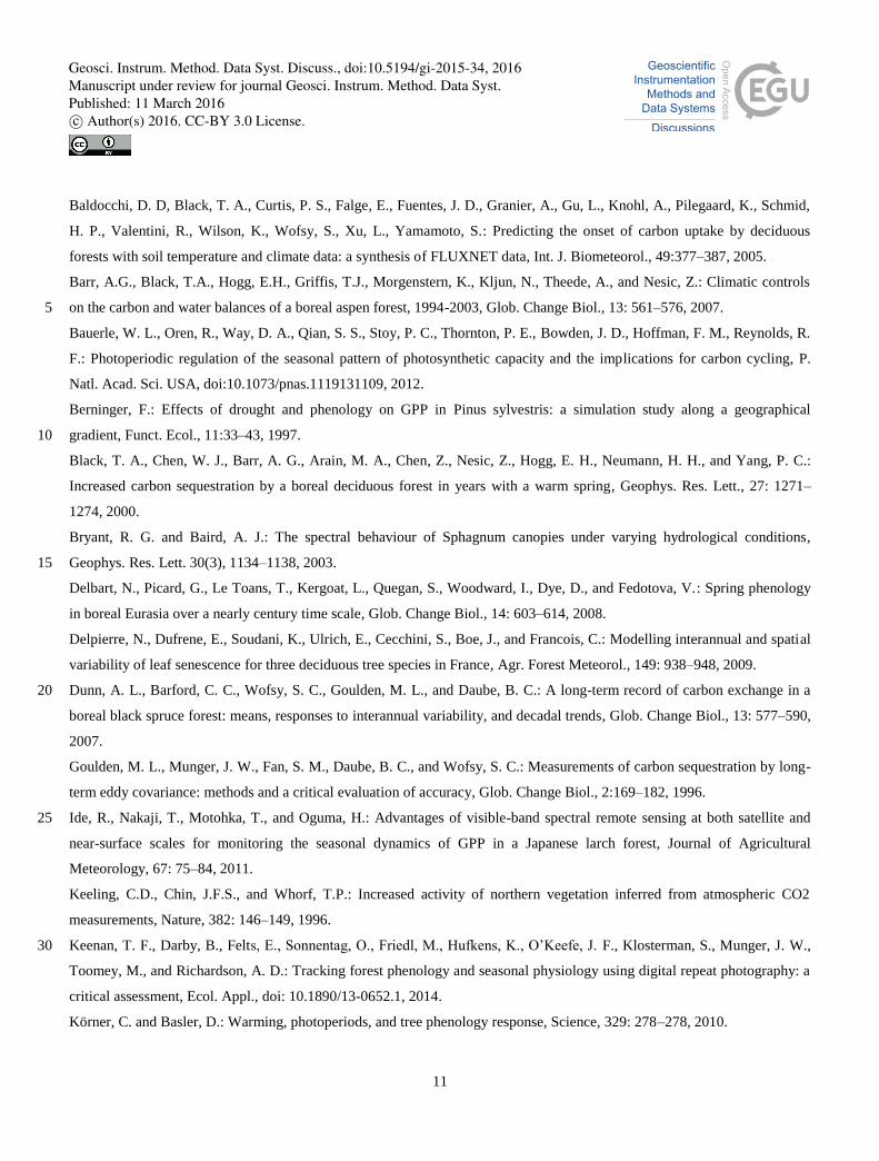
In order to determine the periods when low light levels significantly affect the GCC observation, the mean diurnal GCC

cycles during different months were calculated for the reference plate placed within the tree crown (Fig. 1). These cycles

show that from March to October the mean 30-min GCC values remained stable from 9.00 to 17.00 (local winter time,

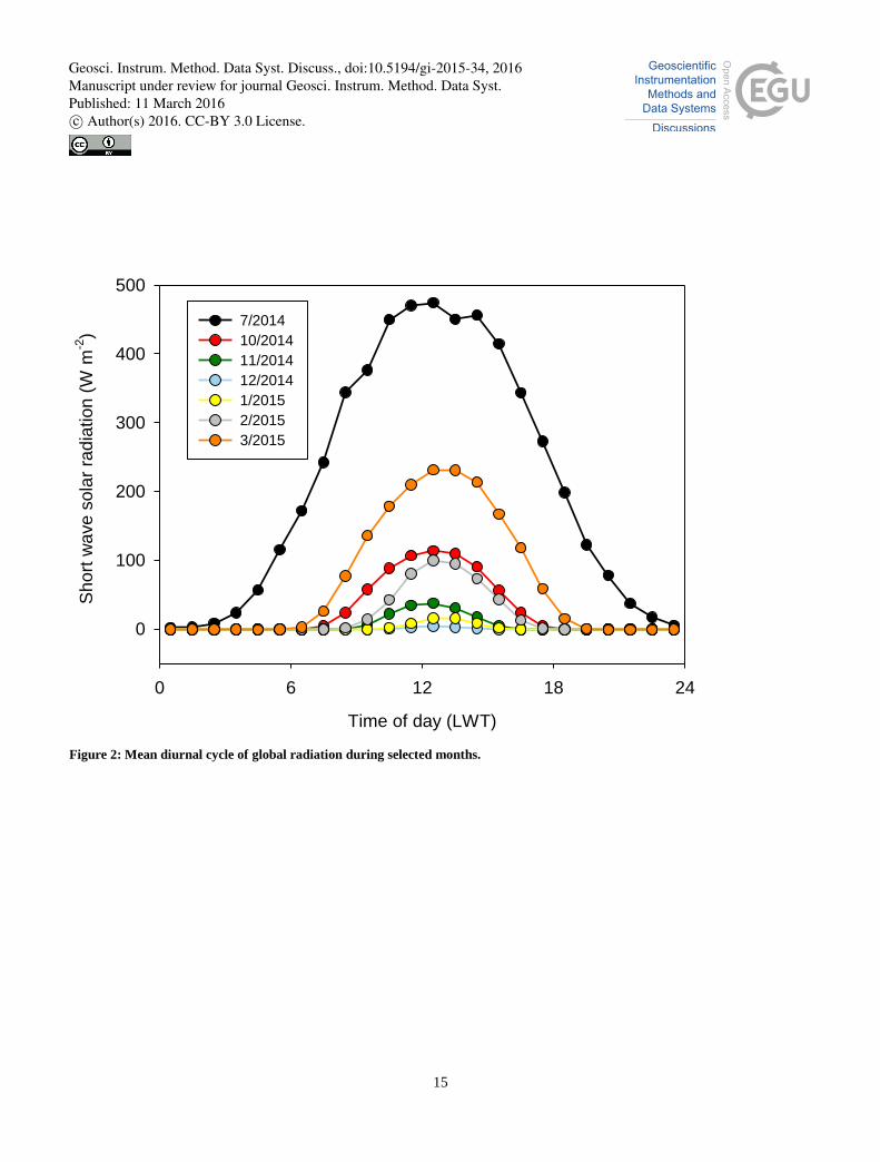
UTC+2). During the other months, the stable period was markedly shorter. In winter, solar radiation is low throughout the 10

day (Fig. 2), which was observed as a decreased GCC level even at noon; in addition, the variance of GCC increased

notably. Similarly, the nocturnal data show a large variance throughout the year, although at these latitudes, i.e. north of the

Arctic circle, it never gets completely dark during the summer months.

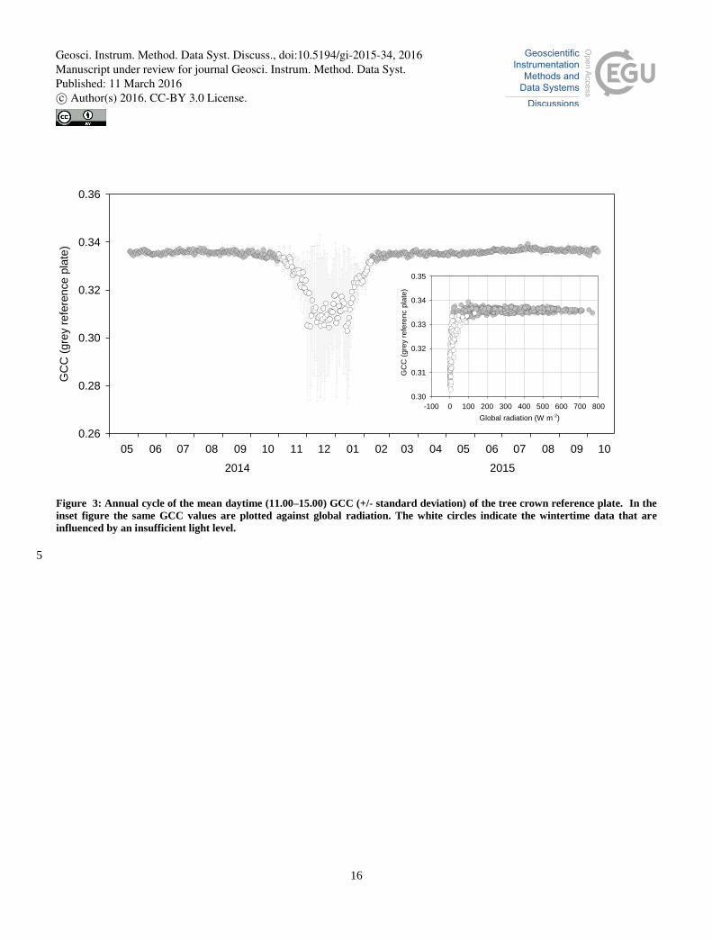
To further illustrate the annual cycle of the reference plate GCC, Fig. 3 shows the mean daytime GCC over a 17-month

period, with the daytime period here limited to 11.00–15.00. The reduction in the mean GCC occurred from November to 15

February, during which period the variance was also increased. This degradation of the signal in insufficient light conditions

must be taken into account, if GCC data are to be used for studying the effect of snow cover, and further investigated if other

measures of greenness are used. However, as the present study aims to observe the phenological development of ecosystems,

we limited the study period to 10 February – 31 October (Fig. 3). During this period, the reference GCC values were stable

varying between 0.332 and 0.339 (with an average of 0.336). The maximum standard deviation for the period was 0.0036. 20

3.1.2 Effect of cloudiness and sun angle

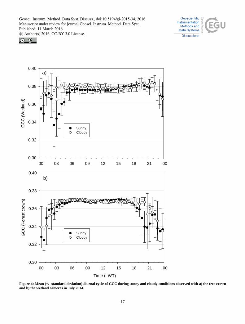
The influence of cloudiness on GCC was estimated from the data collected in July 2014. This particular month was selected

for the test because July represents the lushest growing season and in July 2014 sunny and cloudy days were equally

frequent. Based on the observations of cloudiness (CL, ranging from clear sky with CL = 0 to completely cloudy conditions

with CL = 8), the images were pooled to two contrasting cloudiness groups representing sunny (CL = 0–1) and cloudy (CL 25

= 7–8) conditions. During the daily period selected above (11.00–15.00), the differences in the mean GCC between sunny

and cloudy conditions were statistically insignificant (Mann-Whitney U test) (Fig. 4). The mean GCC difference between the

cloudy and sunny groups was 0.0014 and 0.0011 for the fen and forest, respectively. Sonnentag et al. (2012) found an

equivalently small, though in part statistically significant, difference between the diurnal GCC cycles of sunny and overcast

situations for their deciduous and coniferous forests. 30


7

The dependence of GCC on the sun angle with respect to ROI was also estimated from these data. The difference between

the mean minimum and maximum GCC within the daytime window was 0.0030 and 0.0020 for sunny and cloudy cases,

respectively. This is less than 5% of the seasonal amplitude of the GCC curve (0.069 between May and July) associated with

phenological greening of the fen. At the forest site, the corresponding values were 0.0022 (sunny) and 0.0012 (cloudy) and,

despite the lower annual amplitude (0.024 between May and July), the difference was less than 10% of the seasonal 5

variation.

3.1.3 Selection of the Region of Interest

The sensitivity of the GCC values to the selection of a subarea within an image, i.e. a region of interest, was tested by

comparing the GCC calculated for different vegetation patches. In particular, we wanted to examine, on one hand, if the

forest images are homogeneous and thus insensitive to the ROI definition; on the other hand, the wetland images may 10

provide an opportunity to simultaneously observe various microecosystems incorporated into a single image.

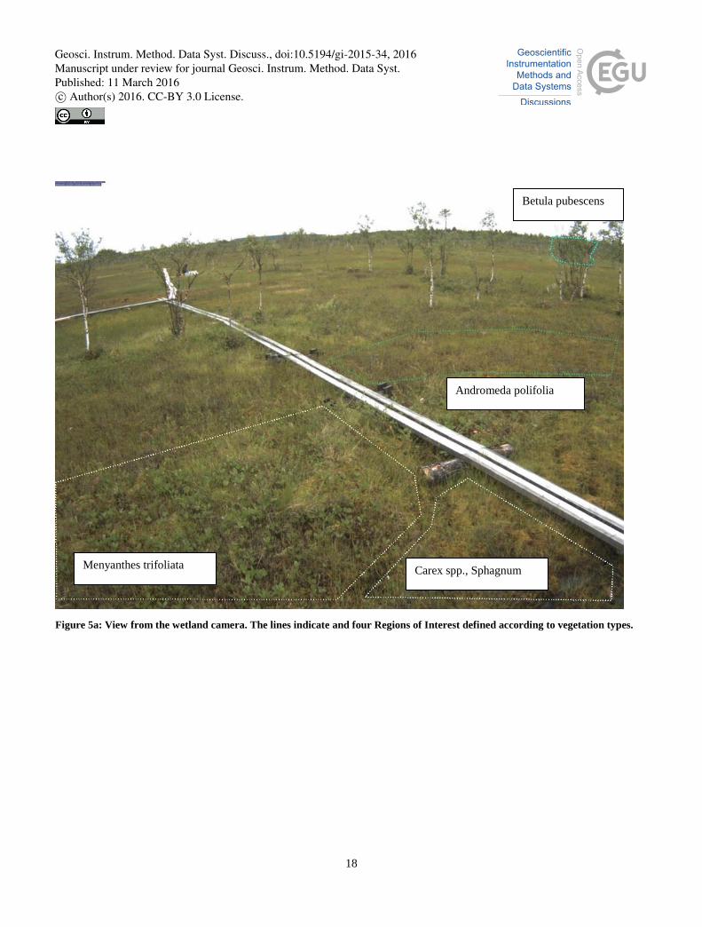
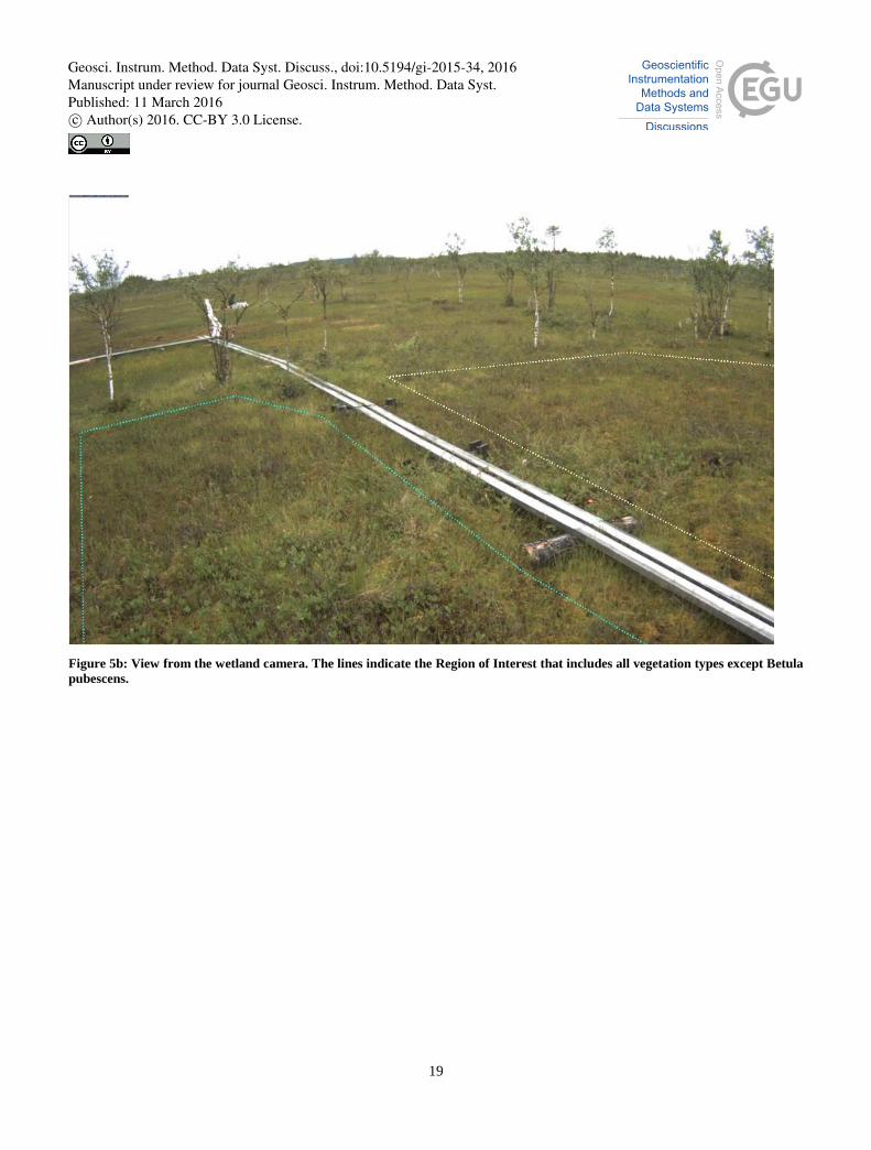
3.1.3.1 Wetland site

GCC was calculated separately for four different, clearly identifiable vegetation types at the wetland site. These vegetation

types were dominated by (1) bog-rosemary (Andromeda polifolia) and other shrubs, (2) sedges (Carex spp.) and Sphagnum

mosses, (3) big-leafed bogbean (Menyanthes trifoliate) and (4) downy birch (Betula pubescens) (Fig. 5a). The first three 15

ROIs include also other ground vegetation, while the fourth ROI is limited to the birch canopy. The GCC values were also

analyzed from a larger area that includes the three first vegetation types (Fig. 5b).

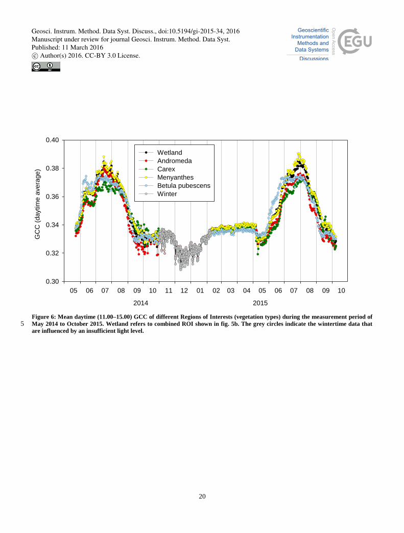
The GCC values of the ROIs defined according to vegetation types showed significant differences in the seasonal cycle, both

in the timing of the major changes in spring and fall and in the magnitude of the maximum GCC (Fig. 6). For example,

downy birch had the fastest growth onset, while the big-leafed bogbean had the largest growing-season maximum. These 20

features suggest that the parallel ROIs should be investigated further in conjunction with small-scale (chamber-based) flux

data. For further analysis, especially for comparing with our ecosystem-scale CO2 flux data, we chose to use the larger area

combining three vegetation types (Fig. 5b).

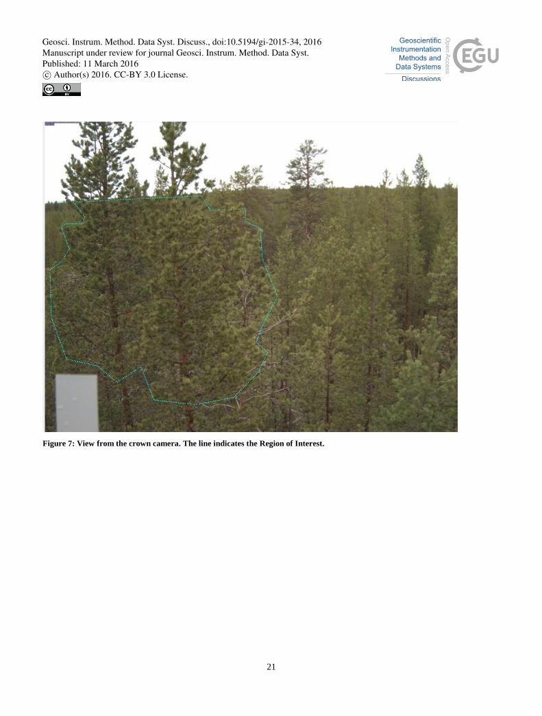
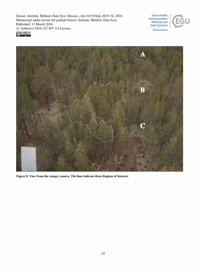
3.1.3.2 Forest site

The forest site had two cameras, one zoomed to the crown of a pine tree (Fig. 7) and the other providing a general view of 25

the canopy (Fig. 8). From the general canopy image, we subjectively selected three separate ROIs with an aim to define

similar homogenous areas of forest canopy (Fig. 8).

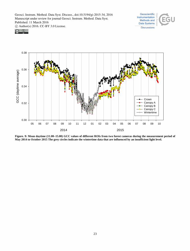
The daily mean GCC values of different canopy ROIs remained very similar throughout the time series (Fig. 9). The GCC

values determined from crown images differed from those from the camera with a general canopy view, most likely because

the cameras had different viewing angles and distances to the object. The contribution of ground is mixed with the canopy 30

signal, which partially explains why the GCC values in the distant canopy camera images are lower than in the crown


8

camera images. In winter, there is more snow visible behind the canopy in the smaller-scale ROIs. Thus, we decided on

using in further analysis only the images from the crown camera.

3.2 Phenological development

3.2.1 Wetland site

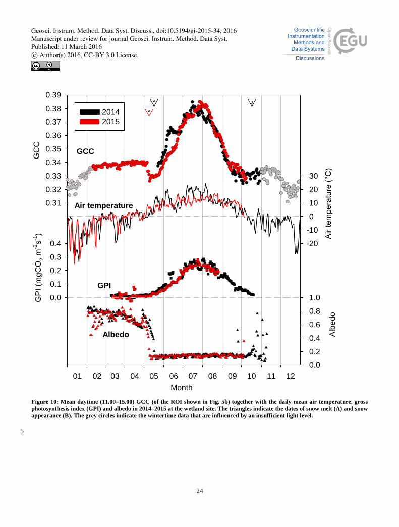
As previously observed by Peichel et al. (2015), at the wetland the growing season is clearly discernable in the development 5

of GCC data (Fig. 10). GCC started to increase as soon as the wetland vegetation started to grow. This growth onset took

place in May after the snow melt, for which the ground albedo provides a sensitive indicator by quantifying the proportion of

incident solar radiation that is reflected back to the atmosphere. However, the onset was preceded by a short period of

reduced GCC values, which were associated with the moist and dark soil.

The warm spells during late May and early June in 2014 induced a rapid emergence and growth of annual plants. Despite the 10

later snow melt that year, by mid-June the growing season had developed much further than in 2015. This difference is

clearly visible in the GCC as well as photosynthetic activity (GPI) data (Fig. 10). The cold period in late June 2014 ceased

this fast development, which is also well reflected in the GCC data that show a stabilization and even a temporary reduction

during that period. GPI shows a similar pattern, highlighting the coherence between the greenness observation and the actual

photosynthetic processes. 15

Following the earlier onset of the growing season in 2014, the peak of plant development was also observed earlier (Fig. 10).

However, the magnitude of the GCC maxima during the two years was very similar. From mid-August to mid-September,

the rate of GCC decline was approximately the same in 2014 and 2015. In mid-September, the slightly higher GCC in 2014

can be attributed to a warm period. By the first sub-zero values in daily mean temperatures, the GCC had decreased to its

minimum value, close to the springtime minimum, and by the snow fall in mid-October it had started increasing towards the 20

level observed for the fully snow-covered conditions in spring.

Previous observations suggest that especially the spring development is well correlated with the GCC of wetlands (Peichel et

al., 2015). Our results support these observations showing a strong relationship between GCC and GPI (Fig. S1), with a

correlation coefficient of 0.90 and 0.92 for the snow-free period in 2014 and 2015, respectively. Especially during the

springtime, the match between the GCC and GPI time series was remarkably close during both years, while in the autumn of 25

2014 GCC lagged slightly behind GPI.

3.2.2 Forest site

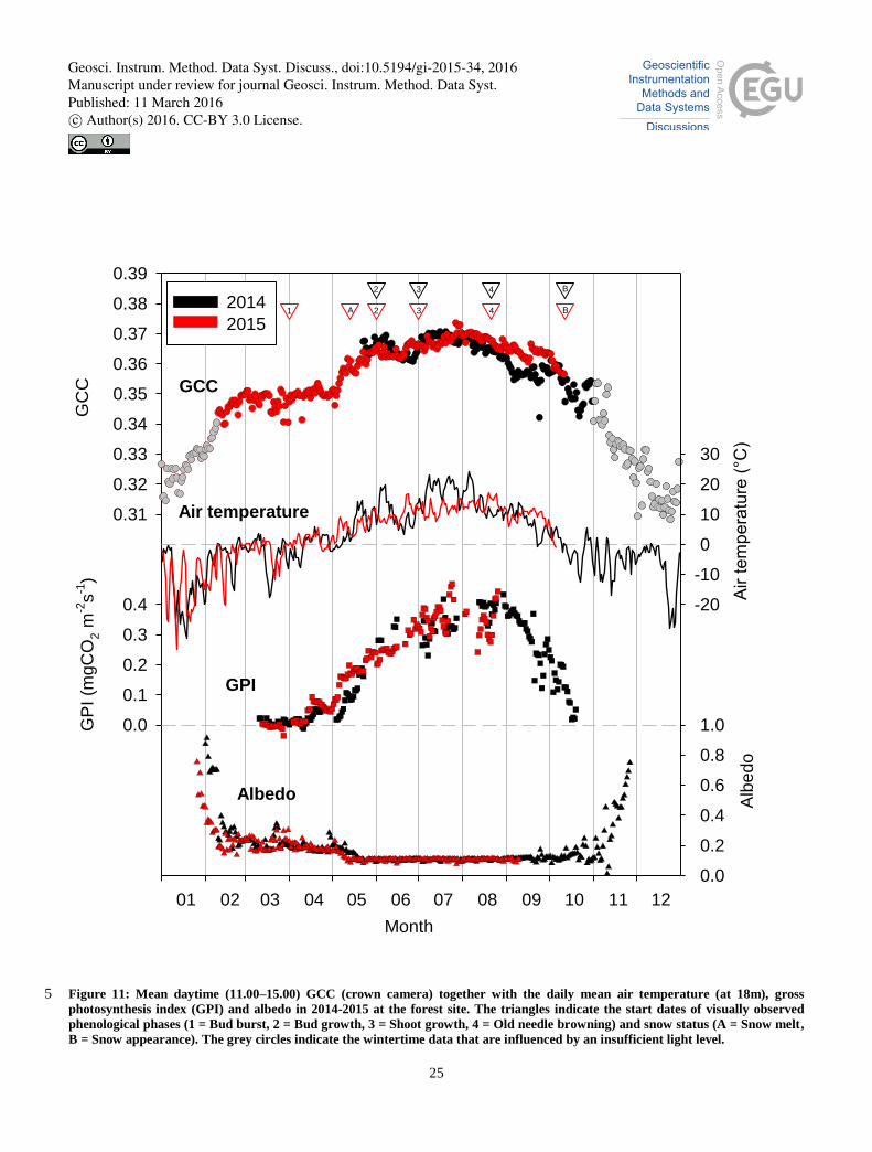
Due to the closeness of the measurement sites, the meteorological conditions in forest were similar to those observed at the

wetland (Figs. 10 and 11). However, the onset of photosynthetical activity differed slightly in the beginning of the growing

season: the warm days of early May 2015 were not observed at the wetland as an GPI increase due to the absence of annual 30

vegetation right after the snow melt, while the photosynthesis of boreal trees is triggered as soon as temperature reaches a


9

sufficient level. Thus the growing season in the forest started earlier in 2015 than in 2014, while that was not the case at the

wetland. Nevertheless, the warm period in late May – early June 2014 also enhanced the forest growth, and by mid-June

both GCC and GPI had surpassed the corresponding level in 2015. The cold period in late June 2014 was again observed as

reduced CO2 uptake and even a clearer reduction in GCC than at the wetland.

Although GCC is generally well correlated with the gross ecosystem photosynthesis during the start of the growing season 5

(Peichel et al., 2015; Toomey et al., 2015), for evergreen needleleaf forests it has been reported that such correlation is often

weaker (Toomey et al., 2015; Wingate et al., 2015). In our data, however, the simultaneous development of GCC and

photosynthesis was evident during the year with spring data available (Fig. S1).

Similarly to the wetland, the maximum GCC level at the forest site did not differ between 2014 and 2015, but this level was

reached slightly earlier in 2014. This was probably due to the higher temperatures during the first part of the growing season. 10

During both years, GCC started decreasing at the same time, i.e. in the end of July. This was slightly earlier than the start of

the senescence detected visually (Phase 4 in Fig. 11). In 2014 there was a clear phase difference between GCC and GPI, the

latter of which stayed at the maximum level until the end of August.

During both years, the photosynthetic activity continues until the end of August, but the interannnual comparison is not

possible here owing to the missing CO2 data in 2015. In both years GCC decreases to the wintertime level in the beginning 15

of October, at the same time as the daily mean temperature decreases below 0C.

In slight contrast to our original hypothesis, the phenological development of the pine canopy could be accurately monitored

with the GCC analysis, even though the GCC changes in forest were subtler than those observed for the wetland vegetation.

This was confirmed by subjectively identifying the phenological stages of the forest from the crown camera pictures (Fig.

11). In 2014, the cameras were installed too late to detect the bud burst, but the GCC time series was consistent with the 20

observation that the buds started their growth in the beginning of June and remained brown until the beginning of July, when

they started to green. The oldest needles in the trees started to brown on around the 20th of August in both years, which is in

accordance with the GCC and GPI data (Fig. 11).

4 Conclusions

The feasibility of digital repeat photography for assessing vegetation phenology was examined in two contrasting high-25

latitude ecosystems. While the seasonal changes in the greenness index GCC are more obvious for those ecosystems where

the vegetation is renewed every year (here an open wetland), seasonal patterns can also be observed in the evergreen

ecosystems (here a coniferous forest).

We examined the applicability and stability of the digital camera system by analyzing the images of a grey reference plate,

which was included in the camera view. Limited solar radiation restricts the use of images during the wintertime as well as 30

during the night-time. At our sites in northern Finland, the daytime radiation levels were sufficient for image analysis from

February to October. During that period, a diurnal window of 11:00–15:00 (local winter time) provides stable GCC data.


10

Outside these time windows, the mean GCC of the grey reference plate was markedly reduced and the noise in GCC

increased.

Our results show that the variability in cloudiness does not play a significant role in the GCC analysis. We pooled reference

plate images to two sets representing sunny and overcast conditions and found no significant difference between these data

sets. Similarly, there was no difference between the data collected before and after noon, indicating that the sun angle had an 5

insignificant influence on the GCC values.

We observed a clear seasonal GCC cycle at both sites. At the wetland, GCC developed in tandem with the daily

photosynthetic capacity estimated from the atmosphere-ecosystem flux measurements. At the forest site, the seasonal GCC

cycle correlated well with the flux data in 2015 but showed some temporary differences in 2014. This difference between the

years was most likely due to meteorological conditions, especially the differences in temperature. 10

In addition to depicting the seasonal course of ecosystem functioning, GCC was shown to respond to physiological changes

on a daily time scale. We observed that a two-week-long cold period in the end of June caused a simultaneous reduction in

GCC and photosynthesis at both sites, and that GCC reflected even shorter-term variations. It seems that our northern sites,

with a short and pronounced growing season, suit especially well for the monitoring of phenological variations with digital

images. 15

Acknowledgements

This work was supported by EU: The installation of the cameras and the development of the Image processing tool

(FMIPROT) was done within MONIMET Project (LIFE12ENV/FI/000409), funded by EU Life+ Programme (2013-2017)

(http://monimet.fmi.fi).

References 20

Ahrends, H. E., Etzold, S., Kutsch, W. L., Stoeckli, R., Bruegger, R., Jeanneret, F., Wanner, H., Buchmann, N., and Eugster,

W.: Tree phenology and carbon dioxide fluxes: use of digital photography for process-based interpretation at the ecosystem

scale, Clim. Res, 39: 261–274, doi: 10.3354/cr00811, 2009.

Aurela, M., Lohila, A., Tuovinen, J.-P., Hatakka, J., Riutta, T., and Laurila, T.: Carbon dioxide exchange on a northern

boreal fen, Boreal Environ. Res., 14: 699–710, 2009. 25

Aurela, M., Tuovinen, J.-P., and Laurila, T.; Net CO2 exchange of a subarctic mountain birch ecosystem, Theor. Appl.

Climatol., 70, 135-148, 2001.

Baldocchi, D.: Assessing the eddy covariance technique for evaluating carbon dioxide exchange rates of ecosystems: past,

present and future, Glob. Change Biol., 9: 479–492, 2003.


11

Baldocchi, D. D, Black, T. A., Curtis, P. S., Falge, E., Fuentes, J. D., Granier, A., Gu, L., Knohl, A., Pilegaard, K., Schmid,

H. P., Valentini, R., Wilson, K., Wofsy, S., Xu, L., Yamamoto, S.: Predicting the onset of carbon uptake by deciduous

forests with soil temperature and climate data: a synthesis of FLUXNET data, Int. J. Biometeorol., 49:377–387, 2005.

Barr, A.G., Black, T.A., Hogg, E.H., Griffis, T.J., Morgenstern, K., Kljun, N., Theede, A., and Nesic, Z.: Climatic controls

on the carbon and water balances of a boreal aspen forest, 1994-2003, Glob. Change Biol., 13: 561–576, 2007. 5

Bauerle, W. L., Oren, R., Way, D. A., Qian, S. S., Stoy, P. C., Thornton, P. E., Bowden, J. D., Hoffman, F. M., Reynolds, R.

F.: Photoperiodic regulation of the seasonal pattern of photosynthetic capacity and the implications for carbon cycling, P.

Natl. Acad. Sci. USA, doi:10.1073/pnas.1119131109, 2012.

Berninger, F.: Effects of drought and phenology on GPP in Pinus sylvestris: a simulation study along a geographical

gradient, Funct. Ecol., 11:33–43, 1997. 10

Black, T. A., Chen, W. J., Barr, A. G., Arain, M. A., Chen, Z., Nesic, Z., Hogg, E. H., Neumann, H. H., and Yang, P. C.:

Increased carbon sequestration by a boreal deciduous forest in years with a warm spring, Geophys. Res. Lett., 27: 1271–

1274, 2000.

Bryant, R. G. and Baird, A. J.: The spectral behaviour of Sphagnum canopies under varying hydrological conditions,

Geophys. Res. Lett. 30(3), 1134–1138, 2003. 15

Delbart, N., Picard, G., Le Toans, T., Kergoat, L., Quegan, S., Woodward, I., Dye, D., and Fedotova, V.: Spring phenology

in boreal Eurasia over a nearly century time scale, Glob. Change Biol., 14: 603–614, 2008.

Delpierre, N., Dufrene, E., Soudani, K., Ulrich, E., Cecchini, S., Boe, J., and Francois, C.: Modelling interannual and spatial

variability of leaf senescence for three deciduous tree species in France, Agr. Forest Meteorol., 149: 938–948, 2009.

Dunn, A. L., Barford, C. C., Wofsy, S. C., Goulden, M. L., and Daube, B. C.: A long-term record of carbon exchange in a 20

boreal black spruce forest: means, responses to interannual variability, and decadal trends, Glob. Change Biol., 13: 577–590,

2007.

Goulden, M. L., Munger, J. W., Fan, S. M., Daube, B. C., and Wofsy, S. C.: Measurements of carbon sequestration by long-

term eddy covariance: methods and a critical evaluation of accuracy, Glob. Change Biol., 2:169–182, 1996.

Ide, R., Nakaji, T., Motohka, T., and Oguma, H.: Advantages of visible-band spectral remote sensing at both satellite and 25

near-surface scales for monitoring the seasonal dynamics of GPP in a Japanese larch forest, Journal of Agricultural

Meteorology, 67: 75–84, 2011.

Keeling, C.D., Chin, J.F.S., and Whorf, T.P.: Increased activity of northern vegetation inferred from atmospheric CO2

measurements, Nature, 382: 146–149, 1996.

Keenan, T. F., Darby, B., Felts, E., Sonnentag, O., Friedl, M., Hufkens, K., O’Keefe, J. F., Klosterman, S., Munger, J. W., 30

Toomey, M., and Richardson, A. D.: Tracking forest phenology and seasonal physiology using digital repeat photography: a

critical assessment, Ecol. Appl., doi: 10.1890/13-0652.1, 2014.

Körner, C. and Basler, D.: Warming, photoperiods, and tree phenology response, Science, 329: 278–278, 2010.


12

Linkosalo, T., Häkkinen, R., Terhivuo, J., Tuomenvirta, H., and Hari, P.: The time series of flowering and leaf bud burst of

boreal trees (1846-2005) support the direct temperature observations of climatic warming, Agr. Forest Meteorol., 149: 453–

461, 2009.

Migliavacca, M., Galvagno, M., Cremonese, E., Rossini, M., Meroni, M., Sonnentag, O., Manca, G., Diotri, F., Busetto, L.,

Cescatti, A., Colombo, R., Fava, F., Morra di Cella, U., Pari, E., Siniscalco, C., and Richardson, A.: Using digital repeat 5

photography and eddy covariance data to model grassland phenology and photosynthetic CO2 uptake, Agr. Forest Meteorol.,

151: 1325–1337, 2011.

Migliavacca, M., Sonnentag, O., Keenan, T. F., Cescatti, A., O’Keefe, J., and Richardson, A. D.: On the uncertainty of

phenological responses to climate change, and implications for a terrestrial biosphere model, Biogeosciences, 9: 2063–2083,

2012. 10

Morisette, J. T., Richardson, A. D., Knapp, A. K., Fisher, J. I., Graham, E. A., Abatzoglou, J., Wilson, B. E., Breshears, D.

D., Henebry, G. M., Hanes, J. M., and Liang, L.: Tracking the rhythm of the seasons in the face of global change:

Phenological research in the 21st century, Front. Ecol. Environ., 7: 253–260, 2009.

Nordli, O., Wielgolaski, F. E., Bakken, A. K., Hjeltnes, S. H., Mage, F., Sivle, A., and Skre, O.: Regional trends for bud

burst and flowering of woody plants in Norway as related to climate change, Int. J. Biometeorol., 52: 625–639, 2008. 15

Peichl, M., Sonnentag, O., and Nilsson, M. B.: Bringing Color into the Picture: Using Digital Repeat Photography to

Investigate Phenology Controls of the Carbon Dioxide Exchange in a Boreal Mire, Ecosystems, 18(1):115–131. doi:

10.1007/s10021-014-9815-z, 2015.

Petach, A., Toomey, M., Aubrecht, D., Richardson, A. D: Monitoring vegetation phenology using an infrared-enabled

security camera, Agr. Forest Met., 195, 143-151, 2014. 20

Pudas, E., Leppälä, M., Tolvanen, A., Poikolainen, J., Venalainen, A., and Kubin, E.: Trends in phenology of Betula

pubescens across the boreal zone in Finland. Int. J. Biometeorol. 52: 251–259, 2008.

Reichstein, M., Falge, E., Baldocchi, D., Papale, D., Aubinet, M., Berbigier, P., Bernhofer, C., Buchmann, N., Gilmanov, T.,

Granier, A., Grünwald, T., Havránková, K., Ilvesniemi, H., Janous, D., Knohl, A., Laurila, T., Lohila, A., Loustau, D.,

Matteucci, G., Meyers, T., Miglietta, F., Ourcival, J.-M., Pumpanen, J., Rambal, S., Rotenberg, E., Sanz, M., Tenhunen, J., 25

Seufert, G., Vaccari, F., Vesala, T., Yakir, D., and Valentini, R.: On the separation of net ecosystem exchange into

assimilation and ecosystem respiration: review and improved algorithm, Glob. Change Biol., 11: 1424–1439, doi:

10.1111/j.1365-2486.2005.001002.x, 2005.

Richardson, A. D., Jenkins, J. P., Braswell, B. H., Hollinger, D. Y., Ollinger, S. V., and Smith, M.-L.: Use of digital webcam

images to track spring green-up in a deciduous broadleaf forest, Oecologia, 152:323–334, doi: 10.1007/s00442-006-0657-z, 30

2007.

Richardson, A. D., Hollinger, D. Y., Dail, D. B., Lee, J. T., Munger, J. W., and O’Keefe, J.: Influence of spring phenology

on seasonal and annual carbon balance in two contrasting New England forests, Tree Physiol., 29: 321–331, 2009.


13

Richardson, A. D., Keenan, T. F., Migliavacca, M., Ryua, Y., Sonnentag, O., and Toomey, M.: Climate change, phenology,

and phenological control of vegetation feedbacks to the climate system, Agr. Forest Meteorol., 169: 156– 173, 2013.

Rosenzweig, C., G. Casassa, D. J. Karoly, A. Imeson, C. Liu, A. Menzel, S. Rawlins, T. L. Root, B. Seguin, and P.

Tryjanowski: Supplementary material to chapter 1: Assessment of observed changes and responses in natural and managed

systems. Climate Change 2007: Impacts, Adaptation and Vulnerability. Contribution of Working Group II to the Fourth 5

Assessment Report of the Intergovernmental Panel on Climate Change, M. L. Parry, O. F. Canziani, J. P. Palutikof, P. J. van

der Linden and C. E. Hanson, Eds., Cambridge University Press, Cambridge, UK, 2007

Sonnentag, O., Chen, J. M., Roberts, D. A., Talbot, J., Halligan, K. Q., and Govind, A.: Mapping tree and shrub leaf area

indices in an ombrotrophic peatland through multiple endmember spectral unmixing, Remote Sens. Environ., 109: 342–360,

2007. 10

Sonnentag, O., Detto, M., Vargas, R., Ryu, Y., Runkle, B. R. K., Kelly, M., and Baldocchi, D. D.: Tracking the structural

and functional development of a perennial pepperweed (Lepidium latifolium L.) infestation using a multi-year archive of

webcam imagery and eddy covariance measurements, Agr. Forest Meteorol., 151: 916–926, 2011.

Sonnentag, O., Hufkens, K., Teshera-Sterne, C., Young, A. M., Friedl, M., Braswell, B. H., Milliman, T., O’Keefe, J., and

Richardson, A. D.: Digital repeat photography for phenological research in forest ecosystems, Agr. Forest Meteorol., 152: 15

159–177, 2012.

Toomey, M., Friedl, M., Frolking, S., Hufkens, K., Klosterman, S., Sonnentag, O., Baldocchi, D., Bernacchi, C., Biraud, S.

C., Bohrer, G., Brzostek, E., Burns, S. P., Coursolle, C., Hollinger, D. Y., Margolis, H. A., McCaughey, H., Monson, R. K.,

Munger, J. W., Pallardy, S., Phillips, R. P., Torn, M. S., Wharton, S., Zeri, M., and Richardson, A. D.: Greenness indices

from digital cameras predict the timing and seasonal dynamics of canopy-scale photosynthesis, Ecol. Appl., 25, 99–115, 20

2015

White, M. A., and Nemani, R. R.: Canopy duration has little influence on annual carbon storage in the deciduous broadleaf

forest, Glob. Change Biol., 9, 2003.

Wingate, L., Ogée, J., Cremonese, E., Filippa, G., Mizunuma, T., Migliavacca, M., Moisy, C., Wilkinson, M., Moureaux, C.,

Wohlfahrt, G., Hammerle, A., Hörtnagl, L., Gimeno, C., Porcar-Castell, A., Galvagno, M., Nakaji, T., Morison, J., Kolle, O., 25

Knohl, A., Kutsch, W., Kolari, P., Nikinmaa, E., Ibrom, A., Gielen, B., Eugster, W., Balzarolo, M., Papale, D., Klumpp, K.,

Köstner, B., Grünwald, T., Joffre, R., Ourcival, J.-M., Hellstrom, M., Lindroth, A., George, C., Longdoz, B., Genty, B.,

Levula, J., Heinesch, B., Sprintsin, M., Yakir, D., Manise, T., Guyon, D., Ahrends, H., Plaza-Aguilar, A., Guan, J. H., and

Grace, J.: Interpreting canopy development and physiology using a European phenology camera network at flux sites,

Biogeosciences, 12, 5995–6015, doi:10.5194/bg-12-5995-2015, 2015. 30


14

Figure 1: Mean diurnal cycle of GCC (+/- standard deviation) of the tree crown reference plate during selected months.

00 03 06 09 12 15 18 21 00

GC

C (

gra

y r

efe

ren

ce

pla

te)

0.24

0.26

0.28

0.30

0.32

0.34

0.36

7/2014

10/2014

11/2014

12/2014

1/2015

2/2015

3/2015

Time of day


15

Figure 2: Mean diurnal cycle of global radiation during selected months.

Time of day (LWT)

0 6 12 18 24

Sh

ort

wa

ve

so

lar

rad

iatio

n (

W m

-2)

0

100

200

300

400

500

7/2014

10/2014

11/2014

12/2014

1/2015

2/2015

3/2015


16

Figure 3: Annual cycle of the mean daytime (11.00–15.00) GCC (+/- standard deviation) of the tree crown reference plate. In the

inset figure the same GCC values are plotted against global radiation. The white circles indicate the wintertime data that are

influenced by an insufficient light level.

5

05 06 07 08 09 10 11 12 01 02 03 04 05 06 07 08 09 10

GC

C (

gre

y r

efe

rence p

late

)

0.26

0.28

0.30

0.32

0.34

0.36

Global radiation (W m-2)

-100 0 100 200 300 400 500 600 700 800G

CC

(gre

y r

efe

renc p

late

)0.30

0.31

0.32

0.33

0.34

0.35

2014 2015


17

Figure 4: Mean (+/- standard deviation) diurnal cycle of GCC during sunny and cloudy conditions observed with a) the tree crown

and b) the wetland cameras in July 2014.

00 03 06 09 12 15 18 21 00

GC

C (

We

tla

nd

)

0.30

0.32

0.34

0.36

0.38

0.40

Sunny

Cloudy

00 03 06 09 12 15 18 21 00

GC

C (

Fo

rest

cro

wn

)

0.30

0.32

0.34

0.36

0.38

0.40

Sunny

Cloudy

a)

b)

Time (LWT)


18

Figure 5a: View from the wetland camera. The lines indicate and four Regions of Interest defined according to vegetation types.

Menyanthes trifoliata

Andromeda polifolia

Carex spp., Sphagnum

Betula pubescens


19

Figure 5b: View from the wetland camera. The lines indicate the Region of Interest that includes all vegetation types except Betula

pubescens.


20

Figure 6: Mean daytime (11.00–15.00) GCC of different Regions of Interests (vegetation types) during the measurement period of

May 2014 to October 2015. Wetland refers to combined ROI shown in fig. 5b. The grey circles indicate the wintertime data that 5 are influenced by an insufficient light level.

2014 2015

05 06 07 08 09 10 11 12 01 02 03 04 05 06 07 08 09 10

GC

C (

daytim

e a

vera

ge)

0.30

0.32

0.34

0.36

0.38

0.40

Wetland

Andromeda

Carex

Menyanthes

Betula pubescens

Winter


21

Figure 7: View from the crown camera. The line indicates the Region of Interest.


22

Figure 8: View from the canopy camera. The lines indicate three Regions of Interest.


23

Figure. 9: Mean daytime (11.00–15.00) GCC values of different ROIs from two forest cameras during the measurement period of

May 2014 to October 2015 The grey circles indicate the wintertime data that are influenced by an insufficient light level.

05 06 07 08 09 10 11 12 01 02 03 04 05 06 07 08 09 10

GC

C (

daytim

e a

vera

ge)

0.30

0.32

0.34

0.36

0.38

Crown

Canopy A

Canopy B

Canopy C

Wintertime

2014 2015


24

Figure 10: Mean daytime (11.00–15.00) GCC (of the ROI shown in Fig. 5b) together with the daily mean air temperature, gross

photosynthesis index (GPI) and albedo in 2014–2015 at the wetland site. The triangles indicate the dates of snow melt (A) and snow

appearance (B). The grey circles indicate the wintertime data that are influenced by an insufficient light level.

5

01 02 03 04 05 06 07 08 09 10 11 12

0.39

0.38

0.37

0.36

0.35

0.34

0.33

0.32

0.31

0.4

0.3

0.2

0.1

0.0

30

20

10

0

-10

-20

1.0

0.8

0.6

0.4

0.2

0.0

2014

2015

GC

CG

PI

(mgC

O2 m

-2s

-1) Air t

em

pe

ratu

re (

°C)

Alb

ed

o

GCC

Air temperature

GPI

Albedo

Month

A

BA


25

Figure 11: Mean daytime (11.00–15.00) GCC (crown camera) together with the daily mean air temperature (at 18m), gross 5 photosynthesis index (GPI) and albedo in 2014-2015 at the forest site. The triangles indicate the start dates of visually observed

phenological phases (1 = Bud burst, 2 = Bud growth, 3 = Shoot growth, 4 = Old needle browning) and snow status (A = Snow melt,

B = Snow appearance). The grey circles indicate the wintertime data that are influenced by an insufficient light level.

01 02 03 04 05 06 07 08 09 10 11 12

0.39

0.38

0.37

0.36

0.35

0.34

0.33

0.32

0.31

0.4

0.3

0.2

0.1

0.0

30

20

10

0

-10

-20

1.0

0.8

0.6

0.4

0.2

0.0

2014

2015

GC

CG

PI

(mgC

O2 m

-2s

-1)

Air t

em

pe

ratu

re (

°C)

Alb

ed

o

GCC

Air temperature

GPI

Albedo

Month

1 2A 3

43

4

B2

B


Digital photography for assessing vegetation phenology in ... · 1 Digital photography for...

Documents

Transcript of Digital photography for assessing vegetation phenology in ... · 1 Digital photography for...