Digital Filters - vscht.czuprt.vscht.cz/prochazka/pedag/lectures/SP5_Filters.pdf · 5. Digital...

5. Digital Filters 71

5

Digital Filters

Any digital systems enabling transformation of a given sequence and using an algorithmic

mathematical approach to such a procedure are often called digital filters. Applications

of these structures cover many areas including system identification and modelling, signal

detection, interference cancelling and system control as well. The following section is

devoted to basic nonadaptive filters while adaptive systems will be discussed further.

5.1 Basic Principles and Methods

A very extensive theory of analog filters has been developed before digital systems started

to be so widely used. It is one of reasons why for many applications prototype analog filters

are designed at first and then transformed to their digital form [5, 23] enabling their more

precise and simple implementation. As such an approach has been described in many

references till now we shall concentrate our attention to the direct digital system design

in most cases.

5.1.1 Digital System Description

A general linear shift invariant discrete system can be described by the difference equation

y(n) +N∑

k=1

a(k)y(n − k) =N∑

k=0

b(k)x(n − k) (5.1)

or according to the mathematical analysis given above by its discrete transfer function

H(z) =Y (z)

X(z)=

N∑k=0

b(k)z−k

1 +N∑

k=1

a(k)z−k

(5.2)

or frequency response

H(ejωk) = H(z) |z=ejωk (5.3)

While the difference equation is essential for transformation of signal {x(n)} to {y(n)}the frequency response function enables the analysis and design of the discrete system

behaviour describing which frequency components of a given signal will be rejected. Basic

ideal frequency responses of various filters are summarised in Fig. 5.1 for digital frequency

ω ∈ 〈0, π). Filter design for approximation of such ideal characteristics presented in

Fig. 5.1 involves

• the estimation of the form of difference equation (5.1) resulting in finite impulse

response (FIR) filter for zero coefficients {a(1), a(2), · · · , a(N)} or infinite impulse

response (IIR) filter

• the evaluation of the difference equation coefficients

These steps are closely connected with demands covering the accuracy of the frequency

response approximation, system stability and its behaviour.

72 5. Digital Filters

FIGURE 5.1. Amplitude frequency characteristics of basic types of filters including (a) idealand real low-pass filter, (b) high-pass, (c) band-pass, and (d) band-stop filters

Example 5.1 Use the discrete system described by equation

y(n) − y(n − 1) + 0.5 y(n − 2) = 0.2 x(n − 1) + 0.2 x(n − 2)

to evaluate its response to the input sequence

x(n) = sin(0.1 n) + sin(2.5 n)

Solution: According to results of Example 3.5 the transfer function of a given system in

the formH(z) = 0.2

z + 1

z2 − z + 0.5implies the amplitude frequency response |H(ejω)| presented in Fig. 5.2 approximating

the low-pass filter. As the spectrum of the given sequence has only one its component in

the system pass-band the difference equation rejects the high frequency signal component

with results given in Fig. 5.2.

5.1.2 Elementary Digital Filters

In various applications very simple digital filters can be used even though their frequency

response is not quite well in comparison with the ideal one.

The moving average system can be described by the difference equation

y(n) =1

N

N−1∑k=0

x(n − k) (5.4)

taking into account N values of a given sequence. As

y(n) =1

N(x(n) + x(n−1) + x(n−2) + · · · + x(n−N +2) + x(n−N+1))

y(n−1) =1

N(x(n−1) + x(n−2) + x(n−3) + · · · + x(n−N+1) + x(n−N))


0 1 2 30

0.5

1

1.5

Frequency

AMPLITUDE FREQUENCY RESPONSE

0 20 40 60 80−2

−1

0

1

2

Index

INPUT SEQUENCE

0 1 2 3

0.1

0.2

0.3

0.4

Frequency

INPUT SEQUENCE SPECTRUM

0 20 40 60 80−2

−1

0

1

2

Index

OUTPUT SEQUENCE

FIGURE 5.2. Amplitude frequency response of the discrete system with the transfer func-tion H(z) = 0.2(z + 1)/(z2 − z + 0.5) and results of its application for processing of sequencex(n) = sin(0.1 n) + sin(2.5 n)

which implies thaty(n) − y(n−1) =

1

N(x(n) − x(n−N))

the discrete transfer function is in the form

H(z) =1

N

zN − 1

zN − zN−1(5.5)

and the frequency response can be expressed after a few mathematical operations (pre-

sented in Example 2.3 in the form

H(ejω) =1

Ne−jω(N−1)/2 sin ωN/2

sin ω/2(5.6)

with ∣∣H(ejω)∣∣ =

1

N

∣∣∣∣sin ωN/2

sin ω/2

∣∣∣∣ (5.7)

Graphic interpretation of this result is presented in Fig. 5.3 for N = 10 showing that

the moving average approximates the low-pass filter with N allowing to change its cutoff

frequency.

The exponential decay system can be described in a similar way by the difference

equation

y(n) =1∑N−1

k=0 v(k)

N−1∑k=0

v(k)x(n − k) (5.8)

for v(k) = v(1)k and v(1) ∈ (0, 1〉 which for v(1) = 1 stands for the moving average in

fact. Asy(n) − v(1) y(n − 1) =

1∑N−1k=0 v(k)

(x(n) − v(N) x(n − N))

the discrete transfer function can be expressed in the form

H(z) =1∑N−1

k=0 vk

zN − v(N)

zN − v(1)zN−1(5.9)



−1

0

1

−1.5−1

−0.50

0.51

1.50

0.2

0.4

0.6

0.8

1

Re(z)Im(z)

0 0.5 1 1.5 2 2.5 30

0.2

0.4

0.6

0.8

1

Frequency


0 0.5 1 1.5 2 2.5 3−3

−2

−1

0

1

2

3

Frequency

PHASE FREQUENCY RESPONSE

FIGURE 5.3. Magnitude and phase frequency response of the moving average system with thetransfer function H(z)=(zN−1)/(N (zN −zN−1)) for N =10 and its sketch in the complex plane

System amplitude frequency response for v(N) << 1 in form∣∣H(ejω)∣∣ ≈ 1 − v(1)√

1 + v(1)2 − 2v(1) cos ω(5.10)

presented in Fig. 5.4 represents the approximation of the low-pass filter again allowing to

use coefficient v(1) to change its cutoff frequency.

0 1 2 30

0.2

0.4

0.6

0.8

1

Frequency

Ampl

itude

EXPONENTIAL DECAY

0 1 2 3−3

−2

−1

0

1

2

3

Frequency

Phas

e

0 1 2 30

0.5

1

1.5

2

Frequency

Ampl

itude

SIGNAL DIFFERENTIATION

0 1 2 3−3

−2

−1

0

1

2

3

Frequency

Phas

e

FIGURE 5.4. Magnitude and phase frequency response of the exponential decay system and thedigital system for signal differentiation.


The signal differentiation described by the difference equation

y(n) = x(n) − x(n − 1) (5.11)

and the discrete transfer function

H(z) = 1 − z−1 (5.12)

has its frequency response in the form

H(ejω) = 1 − e−jω (5.13)

Its magnitude|H(ejω)| =

√(1 − cos ω)2 − sin2 ω = 2 sin(ω/2) (5.14)

presented in Fig. 5.4 represents a very simple approximation of the high-pass filter with

no possiblity of its cutoff frequency change.

5.2 Finite Impulse Response Filter

We shall study now the digital system described by the difference equation

y(n) =P−1∑k=0

h(k) x(n − k) (5.15)

derived from Eq. (5.1) which represents the general moving average system in fact. The

purpose of the following analysis will be in the estimation of P and evaluation of values

{h(0), h(1), · · · , h(P − 1)} standing for the impulse response approximating the ideal

frequency characteristics.

5.2.1 Linear Phase Systems

Definition 5.1 A system with its finite impulse response {h(0), h(1), · · · , h(P − 1)} is

called a linear phase system if its frequency characteristics can be expressed in the form

H(ejωk) =P−1∑n=0

h(n)e−jnωk =∣∣H(ejωk)

∣∣ e−jαωk (5.16)

for ωk = k 2πP

, k = 0, 1, · · · , P − 1.

Systems of this type [23] have an essential role in signal processing applications as

they cause the same delay for all signal frequency components in their passband and

preserve the shape of a given signal. In case that DFT [x(n)] stands for the discrete Fourier

transform of the input sequence the discrete Fourier transform of the system output can

be evaluated in the form

DFT [y(n)] =∣∣H(ejω)

∣∣ e−jαωDFT [x(n)] =∣∣H(ejω)

∣∣ DFT [x(n − α)] (5.17)

It is obvious that if all frequency components of the input signal are in the passband of

the system then y(n) = x(n − α) and the signal is delayed only.

Theorem 5.1 A finite impulse response system of length P is a linear phase system in

case thath(n) = h(P − 1 − n) (5.18)

for n = 0, 1, · · · , P − 1.


Proof: In case of even P it is possible to use the definition of the discrete Fourier transform

to find

H(ejωk =P−1∑n=0

h(n)e−jωkn =

P/2−1∑n=0

h(n)e−jωkn +P−1∑

n=P/2

h(n)e−jωkn

Using further Eq. (5.18) we can evaluate

H(ejωk) =

P/2−1∑n=0

h(n)e−jωkn +

P/2−1∑n=0

h(n)e−jωk(−n+P−1) =

= e−jωk(P−1)/2

P/2−1∑n=0

h(n)(e−jωk(n−(P−1)/2) + e−jωk(−n+(P−1)/2)) =

= e−jωk(P−1)/2

P/2−1∑n=0

2h(n) cos(ωk(n − P − 1

2))

Comparison of the last expression with Eq. (5.16) provides value of

α = (P − 1)/2 (5.19)

Similar results can be obtained for odd P.

5.2.2 Ideal Frequency Response Approximation

Let us assume an ideal low-pass filter according to Fig. 5.1(a) with its linear phase fre-

quency response in the form

H(ejω) =

{e−jαω for 0 < ω < ωc and 2π−ωc < ω < 2π0 for ωc ≤ ω ≤ 2π−ωc

(5.20)

with discrete values of ωk = k 2π/P approaching continuous variable ω for P → ∞. For

this conditions discrete Fourier transform is usually called Fourier transform only and we

can apply it for the approximation of the periodic extension of function (5.20) in the form

H(ejω) =∞∑

n=−∞h(n)e−jnω (5.21)

whereh(n) =

1

2π

∫ 2π

0

H(ejω)ejnωdω (5.22)

It is further possible to evaluate

h(n) =1

2π

∫ ωc

0

e−j(n−α)ωdω +1

2π

∫ ωc

2π−ωc

ej(n−α)ωdω =

=1

2π

[ej(n−α)ω

j(n − α)

]ωc

0

+1

2π

[ej(n−α)ω

j(n − α)

]2π

2π−ωc

=

=1

2πj(n − α)(ej(n−α)ω − 1 + 1 − e−j(n−α)ω) =

sin((n − α)ω)

π(n − α)

Using a finite sequence {h(n)} only limited to P values it is possible to use Eq. (5.19) to

define the linear phase impulse response in the form

h(n) =sin((n − (P − 1)/2)ωc)

π(n − (P − 1)/2)(5.23)


0 2 4 6 8 10 12−0.2

−0.1

0

0.1

0.2

0.3

Index

IMPULSE RESPONSE − P ODD

0 2 4 6 8 10 12−0.2

−0.1

0

0.1

0.2

0.3

Index

IMPULSE RESPONSE − P EVEN

FIGURE 5.5. Finite impulse response {h(n)} for P odd (P = 11) and even (P = 12)

for n = 0, 1, · · · , P − 1. The sketch of such an impulse response for odd and even P is

presented in Fig. 5.5. The magnitude and phase frequency characteristics for a chosen

length P and cutoff frequency is given in Fig. 5.6 confirming the assumption of the linear

phase.

The process of the impulse response restriction to P values only can be looked upon

as the scalar multiplication of the infinite impulse response by the rectangular window

presented in the previous chapter and causing the transition band of length 4π/P [23,

p.201]. The choice of P large enough can restrict the transition band under a given limit.

Comparison of finite impulse response filters for various length P is given in Fig. 5.7

presenting their amplitude frequency responses in dB defined as

H(ejωk) |dB= 20 log(|H(ejωk)|/|H(ejω0)|) (5.24)

with ω0 = 0 for the low-pass filter.

The design procedure of the finite impulse response filter is summarized in Algorithm 5.1

(with the choice of OMS = 0 for the low-pass system).


−1

0

1

−1.5−1

−0.50

0.51

1.50

0.2

0.4

0.6

0.8

1

Re(z)Im(z)

0 0.5 1 1.5 2 2.5 30

0.2

0.4

0.6

0.8

1

1.2

Frequency


0 0.5 1 1.5 2 2.5 3−3

−2

−1

0

1

2

3

Frequency


FIGURE 5.6. Magnitude and phase frequency characteristics of the finite impulse response filterof length P = 64 for cutoff frequency ωc = 0.8 [rad] and its sketch in the complex plane


0 1 2 3−70

−60

−50

−40

−30

−20

−10

0

10

Frequency


P=16

0 1 2 3−70

−60

−50

−40

−30

−20

−10

0

10

Frequency


P=64

FIGURE 5.7. Low-pass amplitude frequency response of the FIR filter limited by the rectangularwindow of various length and cutoff frequency ωc = 0.8 [rad]

5.2.3 Basic Impulse Response Modifications

Finite impulse response filter of the low-pass type with its cutoff frequency ωc derived

above can be very simply modified to form a band-pass filter with its pass-band 2ωc long

and the central frequency ωs. Original impulse response h(0), h(1), · · · , h(P − 1) implies

the magnitude frequency response

∣∣H(ejωk)∣∣ =

∣∣∣∣∣P−1∑n=0

h(n)e−jωkn

∣∣∣∣∣ (5.25)

The shift by ωs in frequency domain presented in Fig. 5.8 implies the band-pass magnitude

frequency response in the form

∣∣H(ej(ωk−ωs))∣∣ =

∣∣∣∣∣P−1∑n=0

h(n)e−j(ωk−ωs)n

∣∣∣∣∣ =

∣∣∣∣∣P−1∑n=0

h̃(n)e−jωkn

∣∣∣∣∣ (5.26)

Algorithm 5.1 Design of the low-pass and band-pass linear phase FIR filter.

• choice of the filter length P , the cutoff frequency OMC of the original low-passfilter and central frequency OMS of the band-pass filter (enabling the low-passfilter design for OMS = 0).

• evaluation of the original impulse response valuesp = 0 : P − 1;h = sin((p − (P − 1)/2) ∗ OMC)./(π ∗ (p − (P − 1)/2));

• definition of the complex impulse response values of the band-pass filterh = h. ∗ exp(j ∗ OMS ∗ p);

• evaluation and plot of a given number of values M of the filter frequency response[hh,w] = freqz (h, [1, zeros(1, P − 1)],M);clg; subplot(211);plot(w, abs(hh)); plot(w, angle(hh));pause

• evaluation of the system output for a given sequence x = [x(1), x(2), · · · , x(N)]for n = P : N

y(n) = h ∗ x(n : −1 : n − P + 1)′

end


LOW−PASS FIR FILTER

−10

1

−1

0

1

0

0.2

0.4

0.6

0.8

1

Re(z)Im(z)

0 0.5 1 1.5 2 2.5 30

0.2

0.4

0.6

0.8

1

Frequency

Ampl

itude

BAND−PASS FIR FILTER

−10

1

−1

0

1

0

0.2

0.4

0.6

0.8

1

Re(z)Im(z)

0 0.5 1 1.5 2 2.5 30

0.2

0.4

0.6

0.8

1

Frequency

Ampl

itude

FIGURE 5.8. Magnitude frequency response of the low-pass and band-pass FIR filter

whereh̃(n) = h(n)ejωsn (5.27)

represents the complex impulse response of the band-pass filter. The design procedure is

summarised in Algorithm 5.1.

It is obvious that owing to symmetry properties of the discrete Fourier transform it is

usually necessary to preserve this symmetry when designing digital filters.

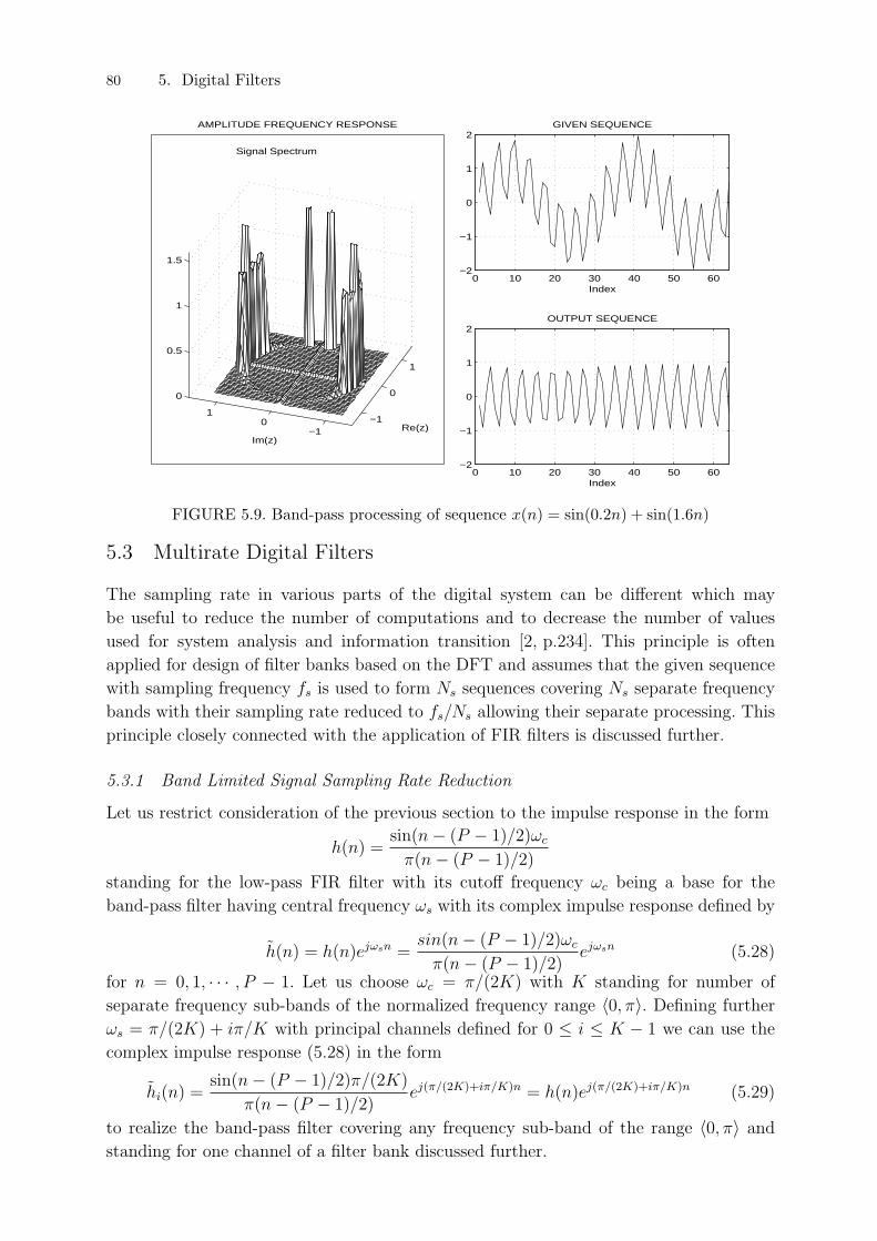
Example 5.2 Use the band-pass FIR filter of length P = 51 to extract the signal in the

frequency band 〈1, 2〉 [rad] from the original sequence

x(n) = sin(0.2n) + sin(1.6n)for n = 0, 1, · · · , N − 1.

Solution: Impulse response of the original low-pass filter for ωc = 0.5 [rad] is given by

Eq. (5.23) which must be then modified by ωs = 1.5 according to Eq. (5.27) to define the

complex impulse responseh̃(n) =

sin((n − (P − 1)/2)ωc)

π(n − (P − 1)/2ejωsn

for n = 0, 1, · · · , P − 1 standing for the band-pass filter in frequency band 〈1, 2〉 [rad]

presented in Fig. 5.9. Owing to symmetry properties it is further necessary to define the

complex impulse response

h̃∗(n) =sin((n − (P − 1)/2)ωc)

π(n − (P − 1)/2e−jωsn

of the complex conjugate filter. The given sequence processing can be based upon Eq. (5.15)

in the formy(n) =

P−1∑k=0

(h̃(k)x(n − k) + h̃∗(k)x(n − k))

for n = P, P + 1, · · · , N − 1.

Further impulse response modifications involve the application of other window de-

scribed till now [23]. Their use mentioned in the previous section enable more efficient

choice of the stop band attenuation and the transition width as well.



Signal Spectrum

−1

0

1

−10

1

0

0.5

1

1.5

Re(z)Im(z)

0 10 20 30 40 50 60−2

−1

0

1

2

Index

GIVEN SEQUENCE

0 10 20 30 40 50 60−2

−1

0

1

2

Index

OUTPUT SEQUENCE

FIGURE 5.9. Band-pass processing of sequence x(n) = sin(0.2n) + sin(1.6n)

5.3 Multirate Digital Filters

The sampling rate in various parts of the digital system can be different which may

be useful to reduce the number of computations and to decrease the number of values

used for system analysis and information transition [2, p.234]. This principle is often

applied for design of filter banks based on the DFT and assumes that the given sequence

with sampling frequency fs is used to form Ns sequences covering Ns separate frequency

bands with their sampling rate reduced to fs/Ns allowing their separate processing. This

principle closely connected with the application of FIR filters is discussed further.

5.3.1 Band Limited Signal Sampling Rate Reduction

Let us restrict consideration of the previous section to the impulse response in the form

h(n) =sin(n − (P − 1)/2)ωc

π(n − (P − 1)/2)

standing for the low-pass FIR filter with its cutoff frequency ωc being a base for the

band-pass filter having central frequency ωs with its complex impulse response defined by

h̃(n) = h(n)ejωsn =sin(n − (P − 1)/2)ωc

π(n − (P − 1)/2)ejωsn (5.28)

for n = 0, 1, · · · , P − 1. Let us choose ωc = π/(2K) with K standing for number of

separate frequency sub-bands of the normalized frequency range 〈0, π〉. Defining further

ωs = π/(2K) + iπ/K with principal channels defined for 0 ≤ i ≤ K − 1 we can use the

complex impulse response (5.28) in the form

h̃i(n) =sin(n − (P − 1)/2)π/(2K)

π(n − (P − 1)/2)ej(π/(2K)+iπ/K)n = h(n)ej(π/(2K)+iπ/K)n (5.29)

to realize the band-pass filter covering any frequency sub-band of the range 〈0, π〉 and

standing for one channel of a filter bank discussed further.


Example 5.3 Evaluate the amplitude frequency response of a FIR band-pass filter of

length P = 64, with K = 4 channels modified by the Hamming window and covering

channels with indices 0 and 3

Solution: Using the window function

W (n) = α − (1 − α) cos(2πn/(P − 1))

for n = 0, 1, · · · , P − 1 and α = 0.54 defined before to modify the complex impulse

response given by Eq. (5.29) it is possible to apply the FFT to obtain results presented in

Fig. 5.10. It is obvious that the passband having bandwidth BW = π/K [rad/s] (equal

to 1/(2K) [Hz]) is represented by M = P/(2K) samples.

Assume a band limited real sequence {y(n)} for n = 0, 1, · · · , N − 1 with its number of

samples N as the integer multiple of P and its spectrum being inside one of the previously

defined principal channel i for i ∈ 〈0, K−1〉 and its complex conjugate. Its spectrum is

defined by means of the discrete Fourier transform for N = P in the form

Y (k) =P−1∑n=0

y(n)e−jkn2π/P (5.30)

for k = 0, 1, · · · , P − 1. Using the inverse discrete Fourier transform it is possible to

evaluate

y(n) =1

P

P−1∑k=0

Y (k)ejkn2π/P (5.31)

Example 5.4 Evaluate the amplitude spectrum of sequence

y(n) = sin(2π0.16n)

for n = 0, 1, · · · , P − 1 and P = 64 and find band-pass filters dividing frequency range

〈0, π〉 to K = 4 sub-bands and including this spectrum.

0 20 40 60

−0.02

0

0.02

0.04

0.06

0.08

0.1

0.12

0.14

Index

IMPULSE RESPONSE

0 1 2 30

0.2

0.4

0.6

0.8

1

1.2ORIGINAL FIR FILTER

π/(2K) Frequency π

0 1 2 30

0.2

0.4

0.6

0.8

1

π/K Frequency π

i=0 i=3

BAND−PASS FIR FILTERS

FIGURE 5.10. Basic impulse response of FIR low-pass filter of length P = 64 and bandwidthBW = 1/(2K) for K = 4 channels modified by the Hamming window (α = 0.54) with itsfrequency response and related band-pass filters spectra covering channels i = 0 and 3.


0 20 40 60−1

−0.5

0

0.5

1

Index

GIVEN SEQUENCE

0 2 4 60

0.2

0.4

0.6

0.8

1

Frequency

SPECTRUM PLOT

i=1 i=6

FIGURE 5.11. The given sequence y(n) = sin(2π0.16n), n = 0, 1, · · · , N − 1 for N = 64 and itsspectrum with frequency responses of two band-pass filters of length P = 64 for K = 4, i = 1and 6.

Solution: Spectrum of the given sequence has its frequency component f = 0.16 included

in channel i = 1 covering the frequency band 〈0.125, 0.25〉 and its complex conjugate with

its index i = 6 according to Fig. 5.11.

The sampling rate reduction by the value K can be realized using each K-th

value of the original sequence only and it is possible to show that this reduced sequence

contains enough information enabling to reconstruct the whole original sequence again.

Theorem 5.2 Assume that a given sequence {y(n)}, n = 0, 1, · · · , P −1 has its spectrum

estimate Y (k), k = 0, 1, · · · , P − 1 for normalized sampling frequency fs = 1 in the range

〈0, 1). Then spectrum of the reduced sequence

{r(n) : r(n) = y(nK)} (5.32)

for n = 0, 1, · · · , 2M − 1 where 2M = P/K stands for an even integer is related to the

original one by equation

R(m) =1

K

K−1∑q=0

Y (m + q 2M) (5.33)

for m = 0, 1, · · · , 2M − 1 covering the frequency range 〈0, 1/K).

Proof: The Fourier transform of sequence {r(n)} defined by (5.32) can be expressed in

the form

R(m) =2M−1∑n=0

y(nK)e−jmn2π/(2M) (5.34)

for m = 0, 1, · · · , 2M − 1. After substitution for y(nK) from Eq. (5.31) we obtain

R(m) =2M−1∑n=0

1

P

P−1∑k=0

Y (k)ejknK2π/P e−jmn2π/(2M)

and taking into account that P = 2MK it is possible to write

R(m) =1

P

P−1∑k=0

Y (k)2M−1∑n=0

ejn(k−m)π/M

As the second sum is nonzero for (k−m) = q 2M only where q is any integer and its value

is equal to 2M = P/K it is possible to simplify the previous equation to the form given

by Eq. (5.33). As stated before the frequency range for the original normalized sampling

frequency fs = 1 is equal to 〈0, fs〉. The subsampling reduces the sampling frequency to

fr = fs/K for sequence {r(n)} and therefore its spectrum covers the frequency range

〈0, fr〉.


Result of this Theorem implies that the Fourier transform (5.30) of the original sequence

having P = 2MK values is reduced by subsampling defined by Eq. (5.32) to 2M values

only which can be evaluated as the average of K original values according to Eq. (5.33).

Example 5.5 Evaluate the spectrum of sequence {r(n)} related to sequence

y(n) = sin(2π0.16n)

studied in Example 5.4 by the reduction coefficient K = 4.

Solution: Results obtained from the definition of the DFT and relation (5.33) are presented

in Fig. 5.12. The original sequence of length P = 64 is reduced to P/K = 2M = 16 values

only. In the same way P = 64 spectrum values covering normalized frequency band 〈0, 1〉are reduced to 2M = 16 values only defining frequency range 〈0, 1/K〉. But owing to the

band limited given sequence it is still possible to distinguish parts due to channel i = 1

and its complex conjugate even for the reduced sequence spectrum. This property is quite

essential for further signal reconstruction.

0 20 40 60−1

−0.5

0

0.5

1

Index

REDUCED SEQUENCE

0 2 4 60

0.2

0.4

0.6

0.8

1

1.2

Frequency

REDUCED SEQUENCE SPECTRUM

0 20 40 60−1

−0.5

0

0.5

1

Index

DILUTED SEQUENCE

0 2 4 60

0.2

0.4

0.6

0.8

1

Frequency

DILUTED SEQUENCE SPECTRUM

FIGURE 5.12. The reduced sequence formed by each K-th value of the original signal (for K = 4)and the diluted sequence with their spectra

Signal reconstruction based on the reduced sequence defined above can be used

to verify that such a sequence can transmit enough information about the original band

limited signal.

Theorem 5.3 Let us dilute the reduced sequence {r(n):r(n)=y(nK)} for n=0, · · ·, 2M−1

where 2M = P/K stands for an even integer by (K − 1) zeros inserted among its each

adjacent values to form sequence

z(n) =

{y(n) for n = 0, K, 2K, · · · , (2M − 1)K0 for other values of n

(5.35)

and let us assume that the spectrum of the original signal {y(n)} is completely contained

in channel i of the band-pass filter defined by its impulse response h̃i(n) given by Eq. (5.29)


and its complex conjugate (related to h̃∗i (n)). Then the original signal can be reconstructed

by sequence

s(n) =P−1∑p=0

z(n−p) (h̃i(n) + h̃∗i (n)) (5.36)

for n = 0, 1, · · · , P − 1.

Proof: The discrete Fourier transform of sequence given by Eq. (5.35) can be evaluated in

the form

Z(k) =

(2M−1)K∑n=0,K,2K,···

y(n)e−jkn2π/P =2M−1∑q=0

y(qK)e−jkqK2π/P

for k = 0, 1, · · · , P − 1. Taking into account that P = 2MK we get sequence

Z(k) =2M−1∑q=0

y(qK)e−jkq2π/(2M) (5.37)

representing the periodic sequence with its period 2M samples long and owing to Eq. (5.34)

standing for the periodic extension of the DFT of the reduced sequence {r(n)}. This fact

implies that the original spectrum of sequence {y(n)} can be evaluated by the scalar

multiplication of spectrum Z(k) by the frequency response of channel i and its complex

conjugate. According to properties of DFT this multiplication corresponds to the convo-

lution in time domain given by Eq. (5.36).

Example 5.6 Evaluate the spectrum of sequence {z(n)} related to sequence

y(n) = sin(2π0.16n)

by Eq. (5.35) and use the convolution with the impulse response h̃i(n) and its complex

conjugate for channel i = 1 to estimate the original sequence.

Solution: Results obtained from the definition of the DFT or relation (5.37) are presented

in Fig. 5.12. It is possible to see that for P = 64 samples of sequence {z(n)} its spectrum

covering the frequency range 〈0, 1〉 [Hz] by P = 64 values is periodic with its period

P/K = 2M = 16 samples long which is equal to frequency band 1/K. Using Eq. (5.36)

it is possible to reconstruct the original sequence in the form presented in Fig. 5.13.

0 20 40 60−1

−0.5

0

0.5

1

Index

RECONSTRUCTED SEQUENCE

0 2 4 60

0.2

0.4

0.6

0.8

1

Frequency

RECONSTRUCTED SEQUENCE SPECTRUM

FIGURE 5.13. The output sequence {s(n)} defined by convolution of the diluted sequence andtwo complex conjugate impulse responses defining frequency bands of the original signal and theoutput sequence spectrum

It is possible to summarize results of the previous mathematical description in the

following way


• The real signal sampled with the frequency fs (according to sampling theorem) being

band limited to the couple of complex conjugate frequency bands each fs/(2K) long

may be subsampled in such way that each K-th sample is used for further processing

only

• The narrover the frequency band is the more substantial subsampling may be applied

allowing lower number of computations involved.

Results given above are very important for design of multirate adaptive filters [2] and

filter banks mention further.

5.3.2 Filter Bank Design

A filter bank [22] is very important signal processing tool usually based on band-pass FIR

filters and often using the multirate principle as well.

Let us assume that we would like to design a filter bank covering frequency range 〈0, π〉by K band-pass filters. Each of these channels can be defined by its complex finite impulse

response given by Eq. (5.29) enabling to find its output for a given sequence {x(n)} in

the form

yi(n) =P−1∑p=0

h̃i(p)x(n − p) (5.38)

Output signal can then be evaluated by equation

y(n) =2K−1∑i=0

viyi(n) (5.39)

where coefficients vi enable to define gain of separate channels and in case of their equal

value vi = 1 for i = 1, 2, · · · , 2K − 1. This structure can be used in case of the adaptive

signal processing as well with individual gains changed during the learning process of the

system.

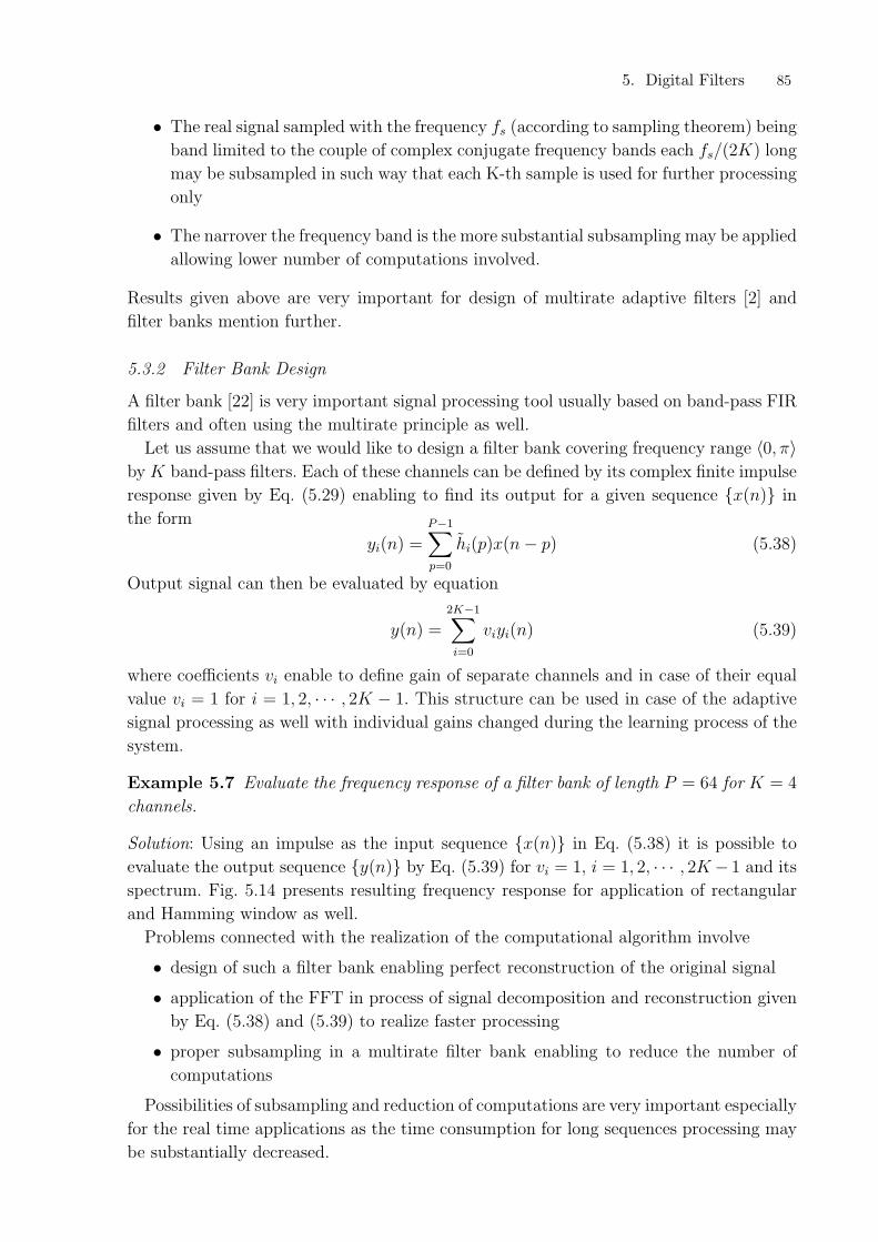
Example 5.7 Evaluate the frequency response of a filter bank of length P = 64 for K = 4

channels.

Solution: Using an impulse as the input sequence {x(n)} in Eq. (5.38) it is possible to

evaluate the output sequence {y(n)} by Eq. (5.39) for vi = 1, i = 1, 2, · · · , 2K − 1 and its

spectrum. Fig. 5.14 presents resulting frequency response for application of rectangular

and Hamming window as well.

Problems connected with the realization of the computational algorithm involve

• design of such a filter bank enabling perfect reconstruction of the original signal

• application of the FFT in process of signal decomposition and reconstruction given

by Eq. (5.38) and (5.39) to realize faster processing

• proper subsampling in a multirate filter bank enabling to reduce the number of

computations

Possibilities of subsampling and reduction of computations are very important especially

for the real time applications as the time consumption for long sequences processing may

be substantially decreased.


FILTER−BANK FREQUENCY RESPONSE

−1

0

1

−1.5−1

−0.50

0.51

1.50

0.2

0.4

0.6

0.8

1

Re(z)Im(z)

0 1 2 30

0.2

0.4

0.6

0.8

1

1.2

Frequency

SPECTRUM − RECTANGULAR WINDOW

0 1 2 30

0.2

0.4

0.6

0.8

1

Frequency

SPECTRUM − HAMMING WINDOW

FIGURE 5.14. Normalized frequency response of K = 4 channel FIR filter bank of length P = 64samples with the use of rectangular and Hamming window function and its sketch in the complexplane.

Example 5.8 Find the fast algorithm evaluating the outputs of all 2K filter bank channels

using the FIR band-pass filters of length P .

Solution: Assuming that P = 2MK and denoting p = q + r2K we can write Eq. (5.38) in

the form

yi(n) =2K−1∑q=0

M−1∑r=0

h̃i(q + r2K)x(n − q − r2K)

Using Eq. (5.29) and owing to periodicity

h̃i(q + r2K) = h(q + r2K)ej(π/(2K)+iπ/K)(q+r2K) =

= h(q + r2K)ejπ(q+r2K)/(2K)ejiq2π/(2K)

and therefore

yi(n) =2K−1∑q=0

ejiq2π/(2K)

M−1∑r=0

h(q + r2K)x(n − q − r2K)ejπ(q+r2K)/(2K) =

=2K−1∑q=0

g(n, q)ejiq2π/(2K) (5.40)

The last expression implies that it is possible for each n to evaluate g(n, q) at first and

then use the inverse DFT for evaluation of yi(n) for all indices i at once. In case that 2K

is a power of 2 the inverse FFT can be applied.

A simple method of the filter bank application based on Eq. (5.40) and (5.39) is pre-

sented in Algorithm 5.2. Further improvement of this algorithm may be achieved by the

use of multirate processing.


Algorithm 5.2 Processing of a sequence {x(n)}2Pn=1 by a filter bank composed of K

FIR filters of length P .

• definition of the filter length P , number of channels K and masking vector v =[v(1), v(2), · · · , v(2K)]

• definition of vector x = [x(1), x(2), · · · , x(2P )]

• definition of the basic impulse response

h = sin((0 : P−1) − (P−1)/2 ∗ π/(2 ∗ K))/(π((0 : P−1) − (P−1)/2))

• for n = P, P +1, · · · , 2P

– evaluation ofg(q) = x((n − q) : −2K : (n − q − (M − 1) ∗ 2K))∗

(h(q : 2K : (q + (M − 1) ∗ 2K)).∗exp(jπ(q + (1 : M − 1) ∗ 2K)/(2 ∗ K)))′;

for q = 0, 1, · · · , 2K − 1 and M = P/(2K) used in Eq. (5.40)

– evaluation of outputs f = [f(1), · · · , f(2K)] of separate bank channels basedon Eq. (5.40)

f = fft(g);

– evaluation of system output according to (5.39)y(n) = sum(f . ∗ v);

The multirate processing can be very efficient as it allows not to follow the sampling

theorem on a channel-by-channel basis as it is sufficient to meet it on the sum of channels.

The evaluation of outputs of K separate channels given by Eq. (5.38) or (5.40) can then be

performed for n = 0, K, 2K, · · · only. The diluted sequences {zi(n)} defined by equation

zi(n) =

{yi(n) for n = 0, K, 2K, · · ·0 for other values of n

(5.41)

similar to Eq. (5.35) can then be used for signal reconstruction. Modifying Eq. (5.36) for

complex signals restricted to one channel only we can use Eq. (5.39) in the form

y(n) =2K−1∑i=0

Bi

P−1∑p=0

zi(n − p)h̃i(p) (5.42)

After a few modifications [34] the FFT can be used in this stage as well.

It is obvious that in case of a complex band limited signal to a single channel even

stronger subsampling may be applied with such a reduction that only each (2K)-th sample

is used.

Example 5.9 Use the filter bank composed of K = 8 FIR filters of length P = 128 to

extract signal components in its channels 1 and 5 for

x(n) = sin(2πf1n) + sin(2πf2n) + 0.2 sin(2πf3n)

for f1 = 0.1, f2 = 0.15, f3 = 0.35 and n = 0, 1, · · · , 2P − 1.


0 20 40 60−2

−1

0

1

2

Time

GIVEN SEQUENCE

0 20 40 60−2

−1

0

1

2

Time

OUTPUT SEQUENCE

0 0.1 0.2 0.3 0.4 0.50

0.2

0.4

0.6

0.8

1

1.2

Frequency

SPECTRUM

i=1 i=5

FIGURE 5.15. Application of a filter bank of length P = 128 and K = 8 channels to processthe given sequence with active channel 1 and 5

Solution: Using the Algorithm 5.2 it is possible to evaluate the system output in form pre-

sented in Fig. 5.15 together with the signal spectrum and filter bank frequency response.

It is possible to see that the middle frequency component is excluded.

The last example presented the non-adaptive application of a filter bank with gains

of separate channels defined in advance. In many other applications their gain can be

adapted with respect to changing conditions in the observed system.

5.4 Infinite Impulse Response Filters

Digital filter is simply specified by the discrete transfer function H(z) with its behaviour

defined by the frequency response H(ejωi) = H(z) |z=ejωi . We shall study now a general

transfer function given as a rational function implying the sequence {h(n)} standing for

the infinite impulse response in the form

H(z) =Y (z)

X(z)=

N∑k=0

b(k)z−k

1 +N∑

k=1

a(k)z−k

=∞∑

k=0

h(k)z−k (5.43)

In comparison with the FIR system not so many coefficients are necessary in this case

enabling to process the given sequence by the difference equation

y(n) = −N∑

k=1

a(k)y(n − k) +N∑

k=0

b(k)x(n − k) (5.44)

On the other hand the problem of stability must be followed for IIR systems and the

phase characteristic is not linear as in FIR processes.


There are various digital filter design procedures enabling to evaluate coefficients of the

transfer function or the difference equation [30, 32, 23] and we shall mention some of them

only.

5.4.1 Least Squares Frequency Characteristics Approximation

Let us suppose a given set of the magnitude frequency response values |Hd(ejωi)| for

frequencies ωi, i = 0, 1, · · · ,M−1. Using the discrete transfer function given by Eq. (5.43)

we can apply the least square method to evaluate its vector of coefficients

w = [b(0), b(1), · · · , b(N), a(1), a(2), · · · , a(N)] (5.45)

minimizing the sum of squared errors defined as

J(w) =M−1∑i=0

(∣∣H(ejωi)∣∣ − ∣∣Hd(e

jωi)∣∣)2

(5.46)

under constraints that all poles of the discrete transfer function are inside the unit circle.

Theorem 5.4 Let us assume the discrete transfer function H(z). Then∣∣H(ejωi)∣∣2 = H(z) H(z−1) |z=ejωi (5.47)

Proof: As H(ejωi) = H(z) |z=ejωi has a complex value for each ωi its magnitude results

from the product of complex conjugate values of H(ejωi) and H(e−jωi).

Using Eqs. (5.43) and (5.47) in Eq. (5.46) we obtain the sum of squared errors in the

form

J(w) =M−1∑i=0

(√ ∑Nk=0 b(k)e−jkωi

∑Nk=0 b(k)ejkωi

(1 +∑N

k=1 a(k)e−jkωi)(1 +∑N

k=1 a(k)ejkωi)− ∣∣Hd(e

jωi)∣∣)2

(5.48)

After the evaluation of the gradient g = ∂J(w)/∂w we can use the steepest descent

method mentioned above to minimize the squared error given by Eq. (5.48). As no control

over stability is applied in this basic method the resulting poles outside the unit circle

must be modified using the following statement.

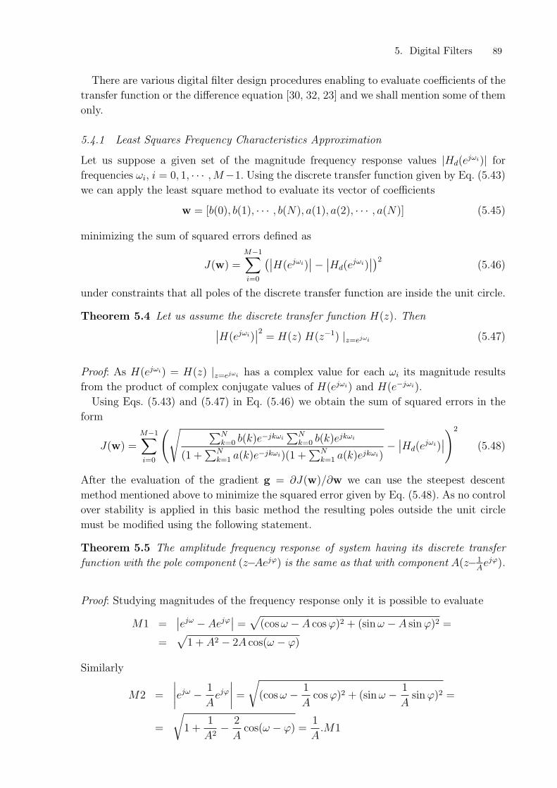
Theorem 5.5 The amplitude frequency response of system having its discrete transfer

function with the pole component (z−Aejϕ) is the same as that with component A(z−1Aejϕ).

Proof: Studying magnitudes of the frequency response only it is possible to evaluate

M1 =∣∣ejω − Aejϕ

∣∣ =√

(cos ω − A cos ϕ)2 + (sin ω − A sin ϕ)2 =

=√

1 + A2 − 2A cos(ω − ϕ)

Similarly

M2 =

∣∣∣∣ejω − 1

Aejϕ

∣∣∣∣ =

√(cos ω − 1

Acos ϕ)2 + (sin ω − 1

Asin ϕ)2 =

=

√1 +

1

A2− 2

Acos(ω − ϕ) =

1

A.M1


Re(z)

Im(z)

(a)

e j*ω

ω

A*e j*φ

φ

Re(z)

Im(z)

(b)

e j*ω

1/A*e j*φ

FIGURE 5.16. Illustration of poles resulting in the same amplitude frequency responses

Both cases are presented in Fig. 5.16.

This statement allows to use reciprocal poles instead of the original ones laying outside

the unit circle which after the gain correction preserve the magnitude response and result

in the stable discrete system.

Example 5.10 Evaluate coefficients of the discrete transfer function (5.43) for N = 3 re-

lated to the difference Eq. (5.44) approximating the ideal low-pass filter with its magnitude

frequency response

Hd(ejωi) =

{1 for i = 0, 1, 2, 30 for i = 4, 5, · · · ,M − 1

where ωi = i πM

, M = 10.

Solution: Using the following notation

g(ωi) =N∑

k=0

b(k)e−jkωi , g∗(ωi) =N∑

k=0

b(k)ejkωi

f(ωi) = 1 +N∑

k=1

a(k)e−jkωi , f ∗(ωi) = 1 +N∑

k=1

a(k)ejkωi

it is possible to express Eq. (5.48) in the form

J(w) =M−1∑i=1

(

√g(ωi)g∗(ωi)

f(ωi)f ∗(ωi)− ∣∣Hd(e

jωi)∣∣)2

with an asteric standing for the complex conjugate. Using further notation given by (5.45)

it is possible to evaluate gradients for k = 0, 1, · · · , N in the form

∂J(w)

∂bk

= 2M−1∑i=1

(√g(ωi)g∗(ωi)


jωi)∣∣) · 1

2

√f(ωi)f ∗(ωi)

g(ωi)g∗(ωi)· e−jkωig∗(ωi) + g(ωi)e

jkωi

f(ωi)f ∗(ωi)

and for k = 1, 2, · · · , N by the following expression

∂J(w)

∂ak

= 2M−1∑i=1

(√g(ωi)g∗(ωi)


jωi)∣∣) · 1

2

√f(ωi)f ∗(ωi)

g(ωi)g∗(ωi)

· −g(ωi)g∗(ωi)[e

−jkωif ∗(ωi) + f(ωi)ejkωi ]

(f(ωi)f ∗(ωi))2

Starting with the initial choice of the parameter vector w = [0.1, 0.2, 0.2, 0.1,−0.7, 0.5,−0.1]

it is possible to use the method of the steepest descent for its updating in the form

wnew = wold − c∂J(w)

∂w(5.49)


0 1 2 3

0

0.2

0.4

0.6

0.8

1

Frequency


it=0 it=5

0 1 2 3−3

−2

−1

0

1

2

3

Frequency



−1

0

1

−1.5−1

−0.50

0.51

1.50

0.2

0.4

0.6

0.8

1

Re(z)Im(z)

FIGURE 5.17. Result of the approximation of the desired frequency response with the processof the amplitude frequency response approximation

Results for the convergence factor c = 0.01 after 5 iterations and system stabilization is

presented in Fig. 5.17.

Computer processing of the discrete transfer function design for a given magnitude fre-

quency response is presented in Algorithm 5.3 using the MATLAB notation. The whole

procedure with further modifications is included in the special function enabling the co-

efficients estimation in the form

[b, a] = yulewalk(N,u,d)

for desired frequency response d defined for frequencies u.

Example 5.11 Use coefficients evaluated in Example 5.10 to process sequence

x(n) = sin(0.3n) + sin(2.2n) (5.50)

Solution: Using difference Eq. (5.44) for N = 3 in the form

y(n) = − a(1)y(n − 1) − a(2)y(n − 2) − a(3)y(n − 3) +

+ b(0)x(n) + b(1)x(n − 1) + b(2)x(n − 2) + b(3)x(n − 3)

it is possible to find solution presented in Fig. 5.18.

5.4.2 Analog System Simulation

As direct digital IIR filter design assumes rather complicated mathematical procedure

analog systems are often used to be transformed into their discrete form. This approach is

described in many books [30, 23, 5] and is based upon the chosen frequency characteristics

in the analytical form and the corresponding transfer function evaluation.

We shall briefly mention the Butterworth filter only with its monotonous magnitude

frequency response and squared gain factor for its low-pass version and normalized unit

sampling in the form


∣∣H(ejω)∣∣2 =

1

1 + tan2N (ω/2)tan2N (ωc/2)

(5.52)

for a given cutoff frequency ωc. This characteristics presented in Fig. 5.19 for various filter

orders N and chosen ωc = 1 approaches an ideal low-pass filter as N gets larger.

Relation ∣∣H(ejω)∣∣2 = H(z) H(z−1) |z=ejω

implies that

H(z).H(z−1) =∣∣H(ejω)

∣∣2ejω=z

=tan2N(ωc/2)

tan2N(ωc/2) + tan2N(ω/2)|ejω=z

As

tan(ω/2) =sin(ω/2)

cos(ω/2)=

1j(ejω/2 − e−jω/2)

ejω/2 + e−jω/2=

1

j

ejω − 1

ejω + 1the previous equation can be rewritten into the form

|H(z)|2 =tan2N(ωc/2)

tan2N(ωc/2) + (−1)N(

z−1z+1

)2N

= tan2N(ωc/2)(z + 1)2N

(z + 1)2N tan2N(ωc/2) + (−1)N(z − 1)2N

Evaluating 2N poles of this rational function it is possible to find [5] that N of them is

inside the unit circle defining the discrete transfer function in the form

H(z) = c(z + 1)N

(z − p(1))(z − p(2)) · · · (z − p(N))(5.53)

Coefficient c can be evaluated to achieve |H(ejω)| = 1 for ω = 0 resulting in equation

c =1

2N(1 − p(1))(1 − p(2)) · · · (1 − p(N)) (5.54)

Evaluating values of the characteristic polynomial it is further possible to define the

discrete transfer function in the form

H(z) = c

1 +

(N1

)z−1 +

(N2

)z−2 + · · · +

(NN

)z−N

1 + a(1)z−1 + · · · + a(N)z−N(5.55)

The whole design procedure is presented in Algorithm 5.4.

Example 5.12 Evaluate coefficients of the low-pass Butterworth filter of order N = 4

having cutoff frequency ωc = 1 and use it to process sequence

x(n) = sin(0.3n) + sin(2.2n)

0 50 100−2

−1

0

1

2

Index

GIVEN SEQUENCE

0 50 100−2

−1

0

1

2

Index

OUTPUT SEQUENCE

FIGURE 5.18. Sequence x(n)=sin(0.3n)+sin(2.2n) before and after processing by an IIR filter


Algorithm 5.3 Infinite impulse response filter design for

H(z) =

N∑k=0

b(k)z−k

1 +N∑

k=1

a(k)z−k

(5.51)

and desired magnitude frequency response

d = [d(1), d(2), · · · , d(M)]

for frequencies in range < 0, π > normalized to range 〈0, 1〉 defined by vector

u = [u(1), u(2), · · · , u(M)]

• choice of initial parameters w = [b, a] for b = [b(0), · · · , b(N)], a =[a(1), · · · , a(N)] and estimation of convergence factor c

• definition of frequency matrix

E =

⎡⎢⎢⎣

1 1 · · · 1exp(−ju1) exp(−ju2) · · · exp(−juM)

· · ·exp(−jNu1) exp(−jNu2) · · · exp(−jNuM)

⎤⎥⎥⎦

• iterative process including

– evaluation of vector g = b ∗ E and g∗ =conj(g)

– evaluation of vector f = [1, a] ∗ E and f∗ =conj(f)

– amplitude frequency response evaluationh =sqrt(g ∗ g∗)./(f ∗ f∗))

– gradient evuluation for k = 0, 1, · · · , N − 1q(k+1)=sum((h−d).∗h.∧(−1).∗(E(k, :).∗g∗+g.∗conj(E(k, :)))./(f ∗ f∗)

– gradient evaluation for k = 1, 2, · · · , Nq(k+N+1)= −sum((h−d). ∗ h. ∧ (−1). ∗ (g. ∗ g∗)./(f . ∗ f∗)...

. ∗ (E(k, :) ∗ f∗ + f∗conj(E(k, :)))

– coefficients updatingw = w − cq; b = w(1 : N + 1); a = w(N + 2 : 2 ∗ N + 1);

• final roots evaluationr =roots(a);

with possible modification for k = 1 : Nif abs(r(k)) > 0

b = b./abs(r(k));r(k) = 1/abs(r(k)∗exp(j∗angle(r(k))));

endand new coefficients definition

a =poly(r);

• final frequency plot presentation[h,u] =freqz(b, a,M); plot(u,abs(h);


0 0.5 1 1.5 2 2.5 30

0.2

0.4

0.6

0.8

1

N=8

4

2

Frequency

BUTTERWORTH FILTER

FIGURE 5.19. Magnitude frequency response of the low-pass Butterworth filter with its cutofffrequency ωc = 1.

Solution: Resulting difference equation

y(i) = −a(1)y(i−1)−· · ·−a(4)y(i−4)+c(x(i)+4x(i−1)+6x(i−2)+4x(i−3)+x(i−4))

(5.56)provides results presented in Fig. 5.20.

Simple modification of the method described above enables realization of the high-pass

or band-pass filter [5] as well.

5.5 Frequency Domain Signal Processing

Signal processing in frequency domain based upon the discrete Fourier transform is often

used for direct modifications of the signal spectrum. This approach assumes no evaluation

of the difference equation coefficients as the filtering process is realized in the frequency

domain only [18, p.292, 369]. Separate steps of the evaluation procedure consist of

• the transformation of the given signal {x(n)}N−1n=0 into the frequency domain by the

DFT

0 20 40 60−2

−1

0

1

2

Index

GIVEN SEQUENCE

0 1 2 30

0.2

0.4

0.6

0.8

1

Frequency

GIVEN SEQUENCE ANALYSIS

0 20 40 60−2

−1

0

1

2

Index

OUTPUT SEQUENCE

0 1 2 30

0.2

0.4

0.6

0.8

1

Frequency

OUTPUT SEQUENCE ANALYSIS

FIGURE 5.20. Results of the given sequence processing by the low-pass Butterworth filter oforder N = 4


Algorithm 5.4 The Butterworth low-pass filter design with its discrete transfer func-tion

H(z) = c(z + 1)N

(z − p(1))(z − p(2)) · · · (z − p(N))(5.57)

• the choice of order N and cutoff frequency ωc

• selection of N poles laying inside the unit circle from poles

p(i) =1 − tan2(ωc/2) + j2 tan(ωc/2) sin(θ(i))

1 − 2 tan(ωc/2) cos(θ(i)) + tan2(ωc/2)

for i = 1, 2, · · · , 2N where

θ(i) =

{(i − 1)π/N for n old(2i − 1)π/(2N) for n even

• definition of coefficient cc =prod(1 − p)/2N

• characteristic polynomial evaluationa = poly(p)

defining the difference equation

y(i) = − a(1)y(i − 1) − a(2)y(i − 2) − · · · − a(N)y(i − N)

+ c(x(i) +

(N1

)x(i − 1) +

(N2

)x(i − 2) + · · · +

(NN

)x(i − N))

• multiplication of the frequency samples {X(k)}N−1k=0 by values of the desired fre-

quency window function {H(k)}N−1k=0 to obtain modified frequency response {Y (k)}N−1

k=0

• the transformation to the time domain through the inverse DFT to obtain signal

{y(n)}N−1n=0

The FFT transform can be applied for this process as well and all necessary steps are

summarised using MATLAB notation in Algorithm 5.5 with presentation in Fig. 5.21.

The frequency window function {H(k)}N−1k=0 representing magnitude frequency response

{|H(ejωk)|}N−1k=0 for ωk = k.2π/N can stand for any type of digital filter and to evaluate real

signal {y(n)}N−1n=0 from a real signal {x(n)}N−1

n=0 it must keep the symmetry properties of

the DFT. It is obvious that it is necessary to use sequence of values with H(k) = H(N−k)

for k = 1, 2, · · · , N − 1.

Example 5.13 Apply the frequency domain signal processing for sequence

x(n) = sin(0.1n) + sin(1.3n) + sin(2n)

where n = 0, 1, · · · , N − 1 and N = 64 using the frequency window function

H(k) =

{1 for k = 0, 1, · · · , 10 and k = 54, 55, · · · , 630 for k = 11, · · · , 53

representing the low-pass filter with cutoff frequency ωc = 10(2π/N).= 0.98.

Solution: Using Algorithm 5.5 with slightly modified sketch of results it is possible to

obtain solution presented in Fig. 5.21 demonstrating that the lowest frequency component

is preserved only.


Algorithm 5.5 Frequency domain processing of signal x = [x(1), x(2), · · · , x(N)] fora window function h = [h(1), h(2), · · · , h(N)].

• definition of vectors x and h

• transformation to the frequency domain: X =fft(x)

• spectrum modification: Y = X. ∗ h

• transformation to the time domain: y =ifft(Y)

• sketch of resultssubplot(221);plot(x);plot(y) % plot of given sequencesf = (0 : N − 1)/N ;plot(f ,real(X), f ,h) % frequency characteristicsplot(f ,real(Y))

5.6 Space-Scale Filtering

5.6.1 Wavelet Coefficients Thresholding

5.6.2 Signal and Image Denoising

0 20 40 60−3

−2

−1

0

1

2

3GIVEN SEQUENCE

0 20 40 60−3

−2

−1

0

1

2

3OUTPUT SEQUENCE

0 0.2 0.4 0.6 0.8 1

0

10

20

30

40GIVEN SEQUENCE SPECTRUM

Frequency0 0.2 0.4 0.6 0.8 1

0

10

20

30

40MODIFIED SEQUENCE SPECTRUM

Frequency

DFT IDFT x(n) y(n)

X(k) Y(k)

H(k)

FIGURE 5.21. Principle of the frequency domain signal processing and its application for thelow-pass filtering of signal x(n) = sin(0.1n)+sin(1.3n)+sin(2n), n = 0, 1, · · · , N −1 for N = 64.


5.7 Summary

Digital filters are used in many engineering applications for non-adaptive and adaptive

signal processing enabling signal modification, its analysis, system identification and pro-

cess control as well. This chapter presented some basic principles and methods only for

signal processing in time and frequency domain.

The main interest has been devoted to finite impulse response filters owing to their not

too complicated design, no problems with their stability and linear phase characteristics.

The use of these systems covers many areas including filter banks studied in this chapter as

well in connection with multirate systems enabling to achieve a very fast signal processing.

Description and design of infinite impulse response filters has been restricted to the

application of the methods of the least squares for the frequency characteristic approxi-

mation and basic analog system simulation.

The application of the DFT for frequency domain signal processing presented a very

efficient method for the signal spectrum modification.

Digital Filters - vscht.czuprt.vscht.cz/prochazka/pedag/lectures/SP5_Filters.pdf · 5. Digital...

Documents

Transcript of Digital Filters - vscht.czuprt.vscht.cz/prochazka/pedag/lectures/SP5_Filters.pdf · 5. Digital...