Digital Filters in Radiation Detection and...

Digital Filters in Radiation Detection and Spectroscopy

Digital Radiation Measurement and Spectroscopy, Oregon State University, Abi Farsoni 1

Digital Radiation Measurement and Spectroscopy

NE/RHP 537

Detector PreamplifierHigh-Speed

ADCHistogram Memory

Digital Pulse Processing

•Digital Spectrometer

Detector PreamplifierAnalog Shaping

AmplifierMultichannel

AnalyzerHistogram Memory

•Classical Spectrometer

Classical and Digital Spectrometers


• Pulse processing algorithm is easy to edit

• No bulky analog electronics

• Post-processing

• Digital pulse shaping

• More cost-effective

• The algorithm is stable and reliable, no thermal noise or other fluctuations

• Effects, such as pile-up can be corrected or eliminated at the processing

level

• Signal capture and processing can be based more easily on coincidence

criteria between different detectors or different parts of the same detector

• Disadvantage: Lack of expert in (Digital Systems + Nuclear Spectroscopy)

Digital Spectrometers: Advantages

Detector PreamplifierHigh-Speed

ADCHistogram Memory

Digital Pulse Processing

•Digital Spectrometer

3 Digital Radiation Measurement and Spectroscopy, Oregon State University, Abi Farsoni

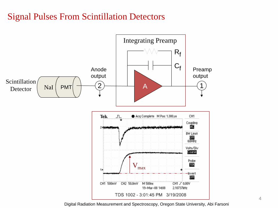
Signal Pulses From Scintillation Detectors

A NaI

Integrating Preamp

PMT

Rf Cf

2

Anode output

Preamp output

1 Scintillation Detector

Vmax


Digital Spectrometers: Digital Pulse Processor (Hardware)

• Analog Conditioning:

o Nyquist filter (𝐹𝑚𝑚𝑚 < 𝐹𝑎𝑎𝑎2

)

o Offset adjustment

o Amplification Gain

• High resolution, fast Analog-to-Digital Convertor (ADC)

• Processing Device:

o FPGA (Field-Programmable Gate Array)

o DSP (Digital Signal Processor)

• Interface:

• USB, PCI, Ethernet 5

A typical FPGA-based digital pulse processor for scintillation detector

Digital Radiation Measurement and Spectroscopy, Oregon State University, Abi Farsoni

Digital Spectrometers: Field-Programmable Gate Array (FPGA)

• FPGAs are an array of programmable logic cells interconnected by a network of wires and configurable switches.

• A FPGA has a large number of these cells available to form multipliers, adders, accumulators and so forth in complex digital circuits.

• FPGAs can be infinitely reprogrammed in-circuit in only a small fraction of a second.

• New FPGA devices provide integrated memory component, to be used as histogram memory.


Trigger

Threshold

Trigger

Enable

Memory Update

Shaping Filter

Histogram Memory

ADC

Detector

FPGA

Peak Detector

Address

Real Counter

Live Counter

Enable

Enable

Digital Spectrometers: Inside the FPGA

Control Unit (State Machine)

Shaping Time

Preamp


Digital Spectrometers: Trigger Module

Fast Triangular Filter

Threshold

From ADC

Trigger Module

Trigger State Machine

A A<B

B

Comparator Trigger Output


Start ?

START

STOP RESET

CNT

WR-BIN

RD-BASE

TRIGGER?

N ?

Pileup

INC-BIN

RD-BIN

SET-ADD PEAK

1. STOP: wait until receiving start pulse 2. RESET: start MCA by resetting counters,

buffers,… 3. START: wait for a trigger pulse 4. RD-BASE: read baseline 5. CNT: wait for N clock cycles 6. PEAK: take a sample from the shaped pulse

(peak) 7. AMP: calculate 𝒂𝒂𝒂 = 𝒂𝒑𝒂𝒑 − 𝒃𝒂𝒃𝒑𝒃𝒃𝒃𝒑

8. SET-ADD: locate and set memory address which corresponds to the pulse amplitude

9. RD-BIN: read current counts from the located address

10. INC-BIN: increment the count by one 11. WR-BIN: write the incremented count to

the same address, go to START state 12. START: wait for another trigger

9

Digital Spectrometers: MCA State Machine

AMP

MCA State Machine with 11 states



convolution x[n] y[n]

• A finite impulse response (FIR) filter is a filter whose impulse response (or

response to any finite length input) is of finite duration, because it settles to zero

in finite time. This is in contrast to infinite impulse response (IIR) filters, which

may have internal feedback and may continue to respond indefinitely.

h[n]

Digital Filters: Finite Impulse Response (FIR) Convolution Operation

10

• For FIR digital filters, the input-output

relation involves a finite sum of products

• Convolution operation defines how the

input signal is related to the output signal


• x[n] is the input signal

• y[n] is the output signal

• h[n] is impulse response (filter coefficients)

• n is the sample number

• N+1 is the filter size 0[ ] [ ] . [ ]

N

ky n h k x n k

=

= −∑

[ ] [0]. [ ] [1]. [ 1] ... [ ]. [ ]y n h x n h x n h N x n N= + − + + −

Digital Filters: Finite Impulse Response (FIR) Convolution Operation (Sum of Products)

11


h[n]


[4] [0]. [4] [1]. [3] [2]. [2] [3]. [1]y h x h x h x h x= + + +

x[0] x[1] x[2] x[3] x[4] x[5] x[6] x[7] x[8] x[9]

h[3] h[2] h[1] h[0]

4

x[0] x[1] x[2] x[3] x[4] x[5] x[6] x[7] x[8] x[9]

h[3] h[2] h[1] h[0]

5

[6] [0]. [6] [1]. [5] [2]. [4] [3]. [3]y h x h x h x h x= + + +

x[0] x[1] x[2] x[3] x[4] x[5] x[6] x[7] x[8] x[9]

h[3] h[2] h[1] h[0]

6

[5] [0]. [5] [1]. [4] [2]. [3] [3]. [2]y h x h x h x h x= + + +

...

...

...

Digital Filters: Finite Impulse Response (FIR) Convolution Operation

Clock #

Output Signal:

12

Filter Coefficients Input Signal

Output Signal:

Output Signal:

[ ] [0]. [ ] [1]. [ 1] [2]. [ 2] [3]. [ 3]y n h x n h x n h x n h x n= + − + − + −

Digital Filters: Finite Impulse Response (FIR) Convolution in Hardware (Realization)

Reg Reg Reg x[n-1] x[n-2] x[n-3]

x[n]

y[n]

h[0] h[1] h[2] h[3]



Digital Filters: Finite Impulse Response (FIR) Moving Average Filter: Noise Reduction

• Consider a digital filter whose output signal y[n] is the average of the four

most recent values of the input signal x[n]:

y[n] = ¼ ( x[n] + x[n-1] + x[n-2] + x[n-3] )

• Such a filter is referred to as a Moving Average Filter and is commonly used

for noise reduction.

• The amount of noise reduction is equal to the square-root of the number of

points in the average. For example, a 100 point moving average filter

reduces the noise by a factor of 10.

14



• In (a), a rectangular pulse is buried in

random noise.

• In (b) and (c), this signal is filtered with 11

and 51 point moving average filters,

respectively.

• As the number of points in the filter

increases, the noise becomes lower; however,

the edges becoming less sharp.

15

• Example of a moving average filter.



But how to implement a Moving Average Filter? Recall the convolution operation (sum of products)

y[n] = ¼ ( x[n] + x[n-1] + x[n-2] + x[n-3] )

In this example, h[n] should be:

h = [ ¼ , ¼ , ¼ , ¼ ]

OR

h = [ 1/N , 1/N , 1/N , 1/N ] , where N is the number of coefficients in the filter

[ ] [0]. [ ] [1]. [ 1] [2]. [ 2] [3]. [ 3]y n h x n h x n h x n h x n= + − + − + −

16


Digital Filters: Finite Impulse Response (FIR) Trapezoidal Filter: Pulse Shaping (for Pre-Amp pulses)

190 195 200 205 210 215 220 225 230 2350

5

10

15

20

25

h = [ .1, .1, .1, .1, .1, .1, .1, .1, .1, .1, 0, 0, 0, 0, 0, -.1, -.1, -.1, -.1, -.1, -.1, -.1, -.1, -.1, -.1 ]

Positive Averaging over L samples

Negative Averaging over L samples Gap

Length (L) = 10

Gap (G) = 5

Signal Input Filter Output

Peaking Time > Charge Collection Time

17

Digital Filters: Finite Impulse Response (FIR) Triangular Filter: Trigger

• Triangular filters with peaking time of 25 nsec and 50 nsec (with T=5 nsec) are:

h1 = [ -1, -1, -1, -1, -1, 1, 1, 1, 1, 1 ]

h2 = [-1, -1, -1, -1, -1, -1, -1, -1, -1, -1, 1, 1, 1, 1, 1 , 1, 1, 1, 1, 1]


• A triangular filter is a special trapezoidal filter with G=0.

Triangular Filter (20 nsec peaking time)


Digital Filters: Finite Impulse Response (FIR) Triangular Filter: Pulse Integration (for Anode pulses)

… -1 … … 1 …

L L

For pulses with negative polarity

For pulses with positive polarity

Pulse Integration Baseline Correction

… 1 … … -1 …

Anode output

Preamp output

Integration Time = L . Sampling Period ;

(The time over which scintillator emits most of its light ~ 99% ~ 4.6 decay time)

NaI: 230 * 4.6 = 1058 nsec

•G=0 (Triangle Filter)

•Unity Coefficients (no normalization)

19

900 950 1000 1050 1100 1150 1200 1250 1300 1350 1400 1450-15

-10

-5

0

5

10

15

20

25

30

35

40

L G Energy Filter (Trapezoidal), L=100,G=20

Trigger Filter (Triangular), L=5,G=0

L

… -1/L … … 1/L … ..0..

Triggering Threshold

Time (nsec)

AD

C U

nits

Trapezoidal and Triangular Filters

Preamp Output

Filter Response


900 950 1000 1050 1100 1150 1200 1250 1300 1350 1400 1450-15

-10

-5

0

5

10

15

20

25

30

35

40

Time (nsec)

AD

C U

nits

V1(max)

V2 (max)

Peak value is sampled

Pile-up is OK if (t2 - t1) > L+G

t2 – t1

Trapezoidal Filters, Pile-up Inspection and Correction

Preamp Output

Filter Response


Digital Filters: Finite Impulse Response (FIR) Trapezoidal and Triangular Filter: Response to Step Function



Digital Filters: Finite Impulse Response (FIR) Some Convolution Practices (with pen and paper!)

0[ ] [ ] . [ ]

N

ky n h k x n k

=

= −∑

Pre-Amp Pulse: x = [1, 1, 1, 1, 1, 1, 3, 3, 3, 3, 3, 3] Digital Filter: h = [ ½, ½, 0, 0, -½, -½ ] Using the Convolution equation, find y[5-11].


h[n]

23



Y[5] = (h[0].x[5-0]) + (h[1].x[5-1]) + (h[2].x[5-2]) + (h[3].x[5-3]) + (h[4].x[5-4]) + (h[5].x[5-5]) Y[5] = (h[0].x[5]) + (h[1].x[4]) + (h[2].x[3]) + (h[3].x[2]) + (h[4].x[1]) + (h[5].x[0]) Y[5] = (0.5 * 1) + (0.5 * 1) + (0 * 1) + (0 * 1) + (-0.5 * 1) + (-0.5 * 1) = 0



24





Y[10] =(h[0].x[10-0]) + (h[1].x[10-1]) + (h[2].x[10-2]) + (h[3].x[10-3]) + (h[4].x[10-4]) + (h[5].x[10-5]) Y[10] = (h[0].x[10]) + (h[1].x[9]) + (h[2].x[8]) + (h[3].x[7]) + (h[4].x[6]) + (h[5].x[5]) Y[10] = (0.5 * 3) + (0.5 * 3) + (0 * 3) + (0 * 3) + (-0.5 * 3) + (-0.5 * 1) = 1

25



Y[11] =(h[0].x[11-0]) + (h[1].x[11-1]) + (h[2].x[11-2]) + (h[3].x[11-3]) + (h[4].x[11-4]) + (h[5].x[11-5]) Y[11] = (h[0].x[11]) + (h[1].x[10]) + (h[2].x[9]) + (h[3].x[8]) + (h[4].x[7]) + (h[5].x[6]) Y[11] = (0.5 * 3) + (0.5 * 3) + (0 * 3) + (0 * 3) + (-0.5 * 3) + (-0.5 * 3) = 0

26

Digital Filters: Infinite Impulse Response (IIR) Trapezoidal shaping using recursive algorithm

27

• Digital filters can be realized in FPGA with minimum resources using recursive algorithm.

• In a recursive algorithm, to synthesis a trapezoidal output y[n] from a step input x[n], we can process the input in two steps.

• In the first step, the step input x[n] is first converted to a bipolar rectangular pulse r[n]. In the second step, r[n] is converted to a trapezoidal output using an accumulator.


28

𝑍 𝑡𝑡𝑡𝑡𝑡𝑡𝑡𝑡𝑡: 𝐻 𝑧 = � ℎ∞

𝑘=−∞

[𝑘]𝑧−𝑘

𝑥 𝑡 = 𝐴 𝑢 𝑡

𝑋 𝑧 = 𝐴

1 − 𝑧−1

𝑡 𝑡 = 𝐴 {𝑢 𝑡 − 𝑢 𝑡 − 𝑘 − 𝑢 𝑡 − 𝑙 + 𝑢 𝑡 − 𝑙 − 𝑘 }

𝑅 𝑧 = 𝐴1

1 − 𝑧−1−

𝑧−𝑘

1 − 𝑧−1−

𝑧−𝑙

1 − 𝑧−1+

𝑧−𝑙−𝑘

1 − 𝑧−1

𝑅 𝑧 = 𝐴

1 − 𝑧−1{1 − 𝑧−𝑘 − 𝑧−𝑙 + 𝑧−𝑙−𝑘}

𝑡 𝑡 = 𝑥 𝑡 ∗ 𝑣[𝑡]

𝑉 𝑧 = 𝑅(𝑧)𝑋(𝑧)

= 1 − 𝑧−𝑘 − 𝑧−𝑙 + 𝑧−𝑙−𝑘

𝑍 𝑡𝑡𝑡𝑡𝑡𝑡𝑡𝑡𝑡 𝑡𝑡 𝑡𝑡 𝑡𝑎𝑎𝑢𝑡𝑢𝑙𝑡𝑡𝑡𝑡 = 𝑊 𝑧 =𝑌(𝑧)𝑅(𝑧)

=1

1 − 𝑧−1




29

• The Z transfer function is: • And finally, by a reverse Z transform we can find the recursive algorithm for the

trapezoidal shaper:

𝒚 𝒃 = 𝒚 𝒃 − 𝟏 + (𝒙 𝒃 − 𝒙 𝒃 − 𝒑 ) − (𝒙 𝒃 − 𝒃 − 𝒙 𝒃 − 𝒃 − 𝒑 )

𝐻 𝑧 =𝑌(𝑧)𝑋(𝑧)

= 𝑉 𝑧 .𝑊 𝑧 =1 − 𝑍−𝑘 − 𝑍−𝑙 + 𝑍−𝑙−𝑘

1 − 𝑧−1

Z-k

+

-

+

- ∑

Z-1

+ Z-l ∑

+ ∑

𝒙 𝒃 − 𝒑

𝒙 𝒃 y 𝒃

𝒙 𝒃 − 𝒃 − 𝒙 𝒃 − 𝒃 − 𝒑

(𝒙 𝒃 − 𝒙 𝒃 − 𝒑 ) − (𝒙 𝒃 − 𝒃 − 𝒙 𝒃 − 𝒃 − 𝒑 )

𝒙 𝒃 − 𝒙 𝒃 − 𝒑

𝒚 𝒃 − 𝟏


Digital Filters in Radiation Detection and...

Documents

Transcript of Digital Filters in Radiation Detection and...