Digital Equalization of Fiber-Optic Transmission System ... · PDF fileiii Abstract In the...

Digital Equalization of Fiber-Optic Transmission System Impairments

i

Digital equalization of fiber-optic transmission system impairments

BY

Ting Luo, B.Eng.

A THESIS

SUBMITTED TO THE DEPARTMENT OF ELECTRICAL & COMPUTER ENGINEERING AND

THE SCHOOL OF GRADUATE STUDIES

OF MCMASTER UNIVERSITY

IN PARTIAL FULFILLMENT OF THE REQUIREMENTS

FOR THE DEGREE OF

MASTER OF APPLIED SCIENCE

Copyright by Ting Luo, September 2011

All Rights Reserved

ii

Master of Applied Science (2010) McMaster University

(Electrical & Computer Engineering) Hamilton, Ontario, Canada

TITLE: Digital equalization of fiber-optic transmission system impairments

AUTHOR: Ting Luo

B.Eng., (Electrical Engineering)

McMaster University, Hamilton, Canada

SUPERVISOR: Dr. Shiva Kumar

NUMBER OF PAGES: x, 53

iii

Abstract

In the past half century, numerous improvements have been achieved to make

fiber-optic communication systems overweigh other traditional transmission systems such

as electrical coaxial systems in many applications. However, the physical features

including fiber losses, chromatic dispersion, polarization mode dispersion, laser phase

noise, and nonlinear effect still post a huge obstruction in fiber-optic communication

system. In the past two decades, along with the evolution of digital signal processing

system, digital approach to compensate these effects become a more simple and

inexpensive solution.

In this thesis, we discuss digital equalization techniques to mitigate the fiber-optic

transmission impairments. We explain the methodology in our implementation of this

simulation tool. Several major parts of such digital compensation scheme, such as laser

phase noise estimator, fixed chromatic dispersion compensator, and adaptive equalizer,

are discussed. Two different types of adaptive equalizer algorithm are also compared and

discussed. Our results show that the digital compensation scheme using least mean square

(LMS) algorithm can perfectly compensate all linear distortion effects, and laser phase

noise compensator is optional in this scheme. Our result also shows that the digital

compensation scheme using constant modulus algorithm (CMA) has about 3~4db power

penalty compare to LMS algorithm. CMA algorithm has its advantage that it is capable of

iv

blind detection and self-recovery, but the laser phase noise compensator is not optional in

this scheme. A digital compensation scheme which combines CMA and LMS algorithm

would be a perfect receiver scheme for future work.

v

Acknowledgement

I would like to express my most sincere gratitude to my supervisor, Dr. Shiva Kumar,

for his insightful advices, patient guidance, and constant encouragement. He has taught

me not only powerful knowledge, but also the way to learn more and to think deeper. I

also would like to thank Dr. Xun Li who referent me to Dr. Shiva Kumar and gave me

many help in my undergraduate and graduate study. Thanks also go to Dr. Wei-Ping

Huang who introduced me into the world of fiber-optic communication system.

I want to appreciate all colleagues of Photonics Research Group and other friends in

both Canada and China for their warm-hearted help and unforgettable friendship.

Last, but not least, I would like to dedicate this work to my dear parents and beloved

for their continued and unconditional love and support.

vi

Notation and abbreviations

3D-IC Three-Dimensional Integrated Circuit

ADC Analog-Digital Converter

ASE Amplified Spontaneous Emission

AWGN Additive White Gaussian Noise

BER Bit Error Rate

CD Chromatic Dispersion

CMA Constant Modulus Algorithm

DCF Dispersion Compensating Fiber

DSF Dispersion-Shifted Fiber

DSP Digital Signal Processing

EDFA Erbium Doped Fiber Amplifier

GVD Group Velocity Dispersion

IC Integrated Circuit

ISI Inter-Symbol Interference

LMS Least Mean Square Algorithm

PDL Polarization Dependent Lose

PLL Phase Lock Loop

PM-QPSK Polarization-Multiplexing QPSK

vii

PMD Polarization Mode Dispersion

QPSK Quadrature Phase-Shift Keying

SOC System-On-A-Chip

SMF Single-Mode Fiber

WDM Wavelength-Division Multiplexing

viii

Contents

Abstract .......................................................................... iii

Acknowledgement .......................................................... v

Notation and abbreviations........................................... vi

Contents ....................................................................... viii

List of Figures ................................................................. x

Chapter 1 Introduction .................................................. 1

1.1 Introduction to Fiber-optic Communication ........................................................... 2

1.2 Distortion effects in Fiber-optic Communication System ...................................... 4

1.3 Thesis Layout .......................................................................................................... 7

Chapter 2 Background ................................................... 8

2.1 Laser Frequency Drift Estimation ........................................................................... 9

2.2 Chromatic Dispersion ............................................................................................. 9

2.3 Polarization Mode Dispersion ............................................................................... 12

2.4 Adaptive Equalization ........................................................................................... 14

Chapter 3 Phase Noise Compensation ........................ 16

3.1 Phase Noise Model ............................................................................................... 17

3.2 Phase Noise Compensation Algorithms ................................................................ 19

3.3 Performance .......................................................................................................... 25

Chapter 4 Dispersion Compensation .......................... 27

4.1 Chromatic Dispersion Model ................................................................................ 28

ix

4.2 Fixed Chromatic Dispersion Compensator ........................................................... 30

4.3 Polarization-Mode Dispersion Model ................................................................... 30

4.4 Adaptive Equalizer ................................................................................................ 31

4.5 System Overview .................................................................................................. 34

4.6 Least Mean Square Adaptive Equalizer ................................................................ 39

4.7 Constant Modulus Adaptive Equalizer ................................................................. 45

4.8 Performance comparison of LMS and CMA ........................................................ 46

Chapter 5 Conclusion and Future Work .................... 48

Bibliography ................................................................. 51

x

List of Figures

Figure 2.1 Illustration of pulse broadening effect due to chromatic dispersion ............ 10

Figure 2.2 Illustration of GVD and pulse broadening effect ......................................... 10

Figure 2.3 Illustration of pulse broadening effect due to PMD..................................... 13

Figure 3.1 Illustration of laser phase noise Wiener process .......................................... 17

Figure 3.2 Illustration of laser phase noise effect ......................................................... 18

Figure 3.3 Illustration of block phase noise compensation scheme. ............................. 24

Figure 3.4 Illustration of compensated received signal. ................................................ 25

Figure 4.1: Illustration of a Gaussian pulses pass through a dispersive fiber ............... 28

Figure 4.2 Structure map of a tap and delay equalizer with feedback. ......................... 31

Figure 4.3 Block diagram of adaptive equalizer for coherent system. .......................... 33

Figure 4.4 Block diagram of receiver layout using DSP compensation scheme .......... 34

Figure 4.5 Constellation map of received signal at different LMS receiver stage. ....... 35

Figure 4.6 Constellation map of received signal at different CMA receiver stage. ...... 38

Figure 4.7 BER vs. launch power optimization. ........................................................... 41

Figure 4.8 BER vs. filter bandwidth ratio optimization ................................................ 43

Figure 4.9 Pulse shape optimization. ............................................................................ 43

Figure 4.10 Illustration of two pulse shapes. ................................................................ 44

Figure 4.11 Performance comparison of CMA and LMS adaptive equalizer ............... 47

Chapter 1

Introduction

M.A.Sc Thesis— Ting Luo McMaster — Electrical and Computer Engineering

2

1.1 Introduction to Fiber-optic Communication

Optical fibers have been employed in telecommunication system for decades and the

market is still growing rapidly nowadays. It becomes more and more popular at both

long-haul and local wired transmission area owning to its many advantages such as high

capacity, low cost, no electromagnetic interferences, and huge bandwidth. While the

demand of fiber-optic system increases dramatically, the relative technology advances

significantly.

By the invention of laser in 1960s, fiber-optic communication system first found a

suitable optical source. Later in 1970, Corning Incorporated demonstrated titanium doped

silica glass with 17dB/Km attenuation and soon the attenuation is reduced to 4dB/Km.

Now there are both suitable optical source and transmission media for the first generation

of fiber-optic communication system. The first generation system operated around 0.8µm

and 45Mbit/s with repeater spacing (repeater is used to regenerate an optical signal by

converting it to an electrical signal, processing that electrical signal and then

retransmitting an optical signal based on the processed electrical signal pattern) in excess

of 10Km. The major limitation of this generation system comes from chromatic

dispersion (CD) which causes significant pulse broadening and thus inter-symbol

interference (ISI).

In order to reduce fiber dispersion effect, single-mode fiber (SMF) was introduced.


3

Comparing to multi-mode fiber, SMF is designed to support only one mode of

propagation light and thus has lower dispersion dramatically. This allows a higher system

symbol rate and longer repeater distance. In 1981, single-mode fiber-optic system

achieved 2Gbit/s at 1.3µm with 44km spacing [1].

Later in 1990, along with the development of silica fibers (low loss) and

dispersion-shifted fiber (DSF) (low dispersion while operating at low loss wavelength

1.5µm) the third-generation fiber-optic communication system emerged. This generation

system was characterized by operating at 1.5µm wavelength region (for latest 0.2dB/Km

loss) and 10Gbit/s with repeater spacing of up to 100Km [2].

The fourth-generation fiber-optic communication system evolution started from 1992

till 2001, owning to the invention of practical optical amplifier (erbium-doped fiber

amplifier (EDFA) more specifically) to replace repeaters and the wavelength-division

multiplexing (WDM) method to increase data capacity. Since 1992, fourth-generation

fiber-optic communication system bit rate start doubling every six months till a bit rate of

10TB/s was achieved by 2001.

Recently, owning to the revolution of integrated circuit (IC) design and the emerge of

system-on-a-chip (SOC) and three-dimensional integrated circuit (3D-IC) level IC, the

cost of high speed DSP system dropped tremendously while the available maximum

processing speed skyrocketed. Researchers started trying to use DSP device to replace the


4

complex and expensive optical device for channel compensation. This approach was first

proved to be feasible in 2003[3], and then various DSP algorithms have been proposed

and tested. Empowered by these technology advancements, fiber optic communication

system has become a versatile, reliable, and cost-efficient wired communication system

solution.

1.2 Distortion effects in Fiber-optic Communication System

As the fiber manufacturing technology advances, many distortion and impairment

effect in fiber-optic communication system decreased significantly. These effects include

but not limit to amplified spontaneous emission (ASE), laser phase noise, chromatic

dispersion (CD), polarization mode dispersion (PMD), and fiber nonlinearity. The first

effect, ASE, sets the hard constraints of any practical fiber-optic communication system.

It imposes the upper limit on system performance. The following three effects, laser

phase noise, CD, and PMD, are the distortion effects that can be compensated. They are

the soft constraints of fiber-optic communication systems. Depending on different

compensator performance, the overall system performance might vary a lot. The last

distortion effect, fiber nonlinearity which is increased as signal power increased, imposes

an upper power constraint to system.

Similar to all other transmission media, optical signal that transmitted in optical fiber

also suffers fiber loss and decays as it is transmitting through the fiber. Although the loss


5

of a fiber is extremely low compared to other transmission media (usually at 0.2dB/km

for 1.55 µm wavelength optical signal nowadays), optical signal decays along fiber link

and will become indistinguishable from noise. Generally, all fiber-optic communication

systems, especially long-haul systems, require optical amplifiers or optical repeaters to

amplify or reconstruct optical signal to ensure its signal-to-noise ratio stays above a

certain recoverable limit. Amplified spontaneous emission noise is the side effect of

employing such optical amplifier in system, and it can be modeled as additive white

Gaussian noise (AWGN).

Laser phase noise comes from the transmitter laser and local oscillator laser (used in

coherent receiver). It can be modeled as a Wiener process, a random walk like white

noise. This effect is hard to compensate by optical device. However, a DSP compensation

device can easily handle this effect. This is first of several prime motivations of using

DSP compensation system in fiber-optic communication system.

Chromatic dispersion (often referred as group velocity dispersion (GVD)) is a

frequency dependent dispersion which causes the optical signal that traveled through fiber

arrived at receiver at different time. This will cause the pulse broadening and

inter-symbol interference which was the major limitation of early fiber-optic

communication system. Although SMF, DSF, and dispersion compensating fiber (DCF)

have been invented to reduce and/or counteract this effect, these compensation


6

approaches are still quite expensive overall. This is another prime motivation of using

DSP compensation system in fiber-optic communication system, to reduce the system

cost.

Polarization mode dispersion (PMD) effect is a fiber only impairment that comes

from the random imperfections and asymmetries of the fiber cross section shape. As the

imperfections exist throughout the whole length of fiber which cause the optical signal in

two polarization travel at different speed and thus cause a random distortion of optical

signal. Because the imperfections are random and slowly time varying (due to thermal

stresses, mechanical stresses, and etc), the PMD effects are random and time-dependent.

Thus, in order to compensate this effect, a compensation device with a feedback

mechanism is required. This is also a prime motivation of using DSP compensation

system in fiber-optic communication system, since an optical device that provides such

function is very expensive and complex.

Fiber nonlinearity describes the optical nonlinearity effect which exhibit at high optic

launch power. When the electric field intensity of electromagnetic wave (light) is

comparable to the inter-atomic electric field of fiber, optical signal will interact with

atoms of fiber and generate new frequency components. Fiber nonlinearity increases as

optical signal power increases. Thus, it enforces an upper limit to the launch power of

fiber-optic communication system.


7

Our major focus in this thesis is about the electronic compensation method for laser

phase noise, chromatic dispersion, and polarization mode dispersion of fiber-optic

communication system. We will explore and provide insight for different DPS

compensation approaches that replace all traditional optical compensation fiber, time lens,

phase lock device and/or optical repeater in once.

1.3 Thesis Layout

The thesis is organized as follows:

In chapter 1, a brief introduction to our topic system is given with the content of each

chapter. A general explanation of system distortion effects is given in section 1.2.

In chapter 2, some background of digital coherent receiver and digital compensation

techniques are discussed.

In chapter 3, a comparison of different laser phase noise compensation scheme will

be shown. The basic concept of laser phase noise model is reviewed. Various

compensation techniques is introduced and compared.

In chapter 4, chromatic dispersion will be introduced to system along with its

compensation approaches. Polarization mode dispersion is also discussed. Both LMS and

CMA adaptive equalizer is reviewed, and their performance is compared.

In chapter 5, the work in this thesis is concluded.

Chapter 2

Background


9

In this chapter, we will review the background of the digital signal processing

algorithm for coherent receivers, especially focusing on the coherent QPSK phase and

polarization diversity receiver. We will discuss the several laser frequency drift (laser

phase noise) compensation techniques, LMS and CMA adaptive equalization technique,

and digital coherent receiver arrangement.

2.1 Laser Frequency Drift Estimation

Estimate and compensate the laser frequency drift is an important step in digital

coherent receiver. Different algorithms were proposed to remove signal phase and thus

estimate laser phase noise [4], [5]. Afterwards, many digital frequency estimation

schemes were proposed such as wiener filtering phase noise estimation[6],

symbol-by-symbol phase noise estimation[7], and block phase noise estimation[8][9].

Accompanied the prevailing M-th power laser phase estimation algorithm, many different

phase unwarping techniques were also proposed to handle phase wrap effect in M-th

power method [6], [8], [10]. The laser frequency drift estimator is discussed in chapter 3

in detail.

2.2 Chromatic Dispersion

The basic physics of chromatic dispersion is the frequency dependence of the

refractive index . Since , the velocity of light at frequency is


10

dependent on its refractive index in the media. The group velocity delay (GVD) of

different spectral components of emitted signal light is determined by the difference of

their refractive index. This frequency dependent dispersion causes the different spectral

components that sent at the same time to arrive at receiver at different time. In a common

communication system where signal pulse is sent consecutively, spectral components of

different pulses overlap due to such spectral broadening effect, and thus causes

inter-symbol interference effect (ISI).

Figure 2.1 Illustration of pulse broadening effect due to chromatic dispersion

Figure 2.2 Illustration of GVD and pulse broadening effect


11

The effects of chromatic dispersion can be modeled by expanding the

mode-propagation constant in a Tayler series about the center frequency as

following

where

|

thus

[

]

0

1

where c is the speed of light in vacuum, and is the first and second order

mode-propagation constant.

Chromatic dispersion is an accumulating effect as signal propagates along fiber.

Usually the propagation distance of the communication channel is known, and thus the

total chromatic dispersion effect can be modeled as following:

.

/

Equation 2.1 can also be expressed in terms of wavelength as following:

.

/


12

where

.

/

D is called the dispersion parameter and is expressed in units of

[27].

2.3 Polarization Mode Dispersion

Another source of pulse broadening is related to fiber birefringence. Any real fibers

have considerable variation in the shape of their core cross section along the fiber length.

They may also sustain non-uniform stress that break the cylindrical symmetry of the fiber.

These random imperfection and asymmetry cause fiber to lose degeneracy between the

orthogonally polarized fiber modes and gain birefringence. The degree of modal

birefringence is defined by

| |

where and are the mode indices for the orthogonally polarized fiber modes. [27]

Birefringence leads to a periodic power leakage between the two polarizations. The

period, referred to as the beat length, is given by

where is the wavelength of the optical signal. In most single mode fibers,

birefringence changes randomly along the fiber in both magnitude and direction. Thus,


13

optical signal travelled through fiber with linear polarization reaches a state of random

polarization. Furthermore, if both polarization components are excited by input signal

pulse different frequency spectral component of the signal pulse acquire different

polarization states, and thus lead to pulse broadening. [27]

Figure 2.3 Illustration of pulse broadening effect due to PMD

In a fiber with constant birefringence, pulse broadening effect can be modeled as

following

|

| | |

It is a bit different for conventional fiber in which birefringence varies randomly along

the fiber. In this case, the pulse broadening effect cannot be estimated by previous

formula, and only statistical mean dispersion can be calculated as follow

⟨ ⟩ √


14

where is the PMD parameter. Measured values of vary in the range between

0.01 √ to 10 √ .

These distortion effects are called the polarization mode dispersion and have been

studied extensively because it is a major performance degradation factor. In our

simulation, we have taken both polarization power leakage and differential group delay

variations into consideration.

2.4 Adaptive Equalization

In order to use digital coherent receiver to replace the former optical compensation

device and receiver, a suitable equalization scheme is required to compensate other linear

impairment effects such as PMD/PDL, CD. Several single channel (PMD/PDL ignored,

no polarization multiplexing is used) compensation schemes using adaptive equalizer

were introduced [6] [11]. For polarization multiplexed system, a modified scheme was

proposed theoretically in [12] with fixed tap weight. Later, adaptive adjusted tap weight

has been used in [7] (theoretical analysis) and [13]-[15] (experimental work). LMS

algorithm was used to adaptive update tap weight in order to compensate time-varying

impairment effects in [7], [13] and [15]. In [14] constant modulus algorithm (CMA [16]

[17]) is employed in steady of LMS. Afterwards, several slightly modified schemes were

described in [18]-[20]. These schemes add a complex FIR filters to compensate bulk CD

before adaptive equalizer. In [19] and [20], CMA algorithm is used in training stage for


15

initial tap weight conversion, and then LMS algorithm is used in receiving stage.

Chapter 3

Phase Noise Compensation


17

3.1 Phase Noise Model

Laser phase noise is come from the non-ideal oscillators used at both transmitter and

receiver side. Laser phase noise is a continuous-time stochastic Wiener process, which is

like a random walk in phase domain. The instantaneous frequency of a laser is modeled as

a white Gaussian noise. Therefore, the phase noise becomes a Wiener process.

Figure 3.1 Illustration of laser phase noise Wiener process, 25GHz system, laser

line-width = 10 MHz, 2.5 Mbits simulation length (0.1ms duration)

As shown in figure 3.1, the accumulation of phase noise is unbounded and thus could


18

cause a complete loss of signal phase information. In most fiber-optic communication

schemes, this effect is vital and must be compensated.

In this chapter, we assume all other impairments other than laser phase noise and

optical amplifier noise have been perfectly compensated. In this case, we will have

following formula:

( )

Where Rk is the received signal symbol at kΔT, ΔT is the sampling period, and Sk is

the modulated signal. Total phase noise off-set of previous symbol is θk-1, and additive

phase noise in k-th time interval is Δθk. The additive channel noise(ASE) is represented

as Nk.

(a) (b) (c)

Figure 3.2 Illustration of laser phase noise effect, 25GHz system, (a) laser line-width = 0

kHz, 300kbits length (1 ms) (b) laser line-width = 10 MHz, 25kbits length (1 s) (c) laser

line-width = 10 MHz, 2.5 Mbits length (0.1 ms)

Comparing figure 3.2 (b) to (a), we find out that laser phase noise will cause MPSK


19

signal phase shift and thus degrade the system performance. From the difference of figure

3.2 (b) and (c), we observed the impact of the phase shift accumulation effect over time.

It is obvious that laser phase noise has to be compensated or eventually the receiver will

lose track of correct signal-symbol mapping.

3.2 Phase Noise Compensation Algorithms

There are two different approaches to compensate laser phase noise, by using phase

lock loop (PLL) device to track signal phase in optical domain or using coherent detection

with DSP device to compensate it in electrical domain. In this chapter, we will focus on

DSP approach in electrical domain and discuss several different possible algorithms.

3.2.1 M-th Power Method

The first step of any DSP compensation algorithm is to isolate phase noise from

signal message phase. Assuming that we are using M-PSK modulation scheme, the signal

message phase is *

+, where Sk is modulated signal, =0,1,2, … ,M-1, M

is the number of phase levels. Since , where m=0,1,2,… , and

√ , we can only remove the signal message phase and thus isolate phase noise. This

is achieved by multiplying the received signal phase by M and then take exponential

function of the phase,

{[ ] }

{ { } }


20

, *

+ -

{[ ] }

( )

where θk is total laser phase noise, is total effective phase noise. When Nk=0,

.

However, the computation cost of this method is relatively high (70% higher in

computation time than equation 3.3) which lead us to introduce a small modification to

this method (equation 3.3) [21].

Thus, from equation 3.3, we can estimate current phase noise from lasers and channel.

Assuming that

( )

to ensure that we can track signal phase noise increment sample by sample, this method

can perfectly remove signal message phase from received signal and track signal phase

noise increment at each sample. It enables the DSP device to reconstruct the phase noise

model and thus compensate it.

Although M-th power method can perfectly remove signal message phase, it will also

remove any

component in phase noise and cause a phase wrapping effect to wrap

phase noise into

] range. We need a phase unwrapping routine to track this


21

effect and reverse it [22], [23]. Let current total phase noise to be

(3.5)

, phase wrapping effect will crop the

part, which is similar to signal message, and

output . is a integer that will minimize . Obviously, this

effect needs to be undone to prevent undesirable phase jump when changes.

3.2.2 Phase Unwrapping

As we discussed in section 3.1, laser phase noise is an accumulating effect and its

absolute value might and will eventually become larger than

. In order to still keep

track of phase noise after using M-th power method, we also need to monitor any change

of value p in equation 3.5. In order to achieve this objective, we employed the maximum

likelihood principle. First we assume that , which equals to , will always

lesser than

before taking M-power and being wrapped. Based on this assumption,

with following formula

[

(

)]

We are able to unwrap phase noise to its original phase index and avoid phase jump error.

However, the first assumption that we made is not necessary to be true in practical

system, especially looking it over large time span or in an extremely noisy system. As

stated in section 3.2.1, total phase noise in received signal comes from not only laser


22

phase noise, but also additive channel white noise. In fact, in a noisy system, total phase

noise in received signal mainly comes from channel noise. The combined effect of laser

phase noise and channel noise will almost for sure result in a violation of our assumption

within every millisecond or even lesser. We want to ensure that our unwrapping routine

will not introduce extra error when our first assumption is violated. This goal is achieved

by intentionally introducing a maximum compensation limit within a certain time interval.

This prevents the fast-varying zero-mean component of phase noise, which comes from

channel noise, from destroying our signal reception. In our software and simulations, this

limit is set to two times of the average of total laser phase noise that will be additively

introduced at current laser line-width configuration.

3.2.3 Phase Noise Compensation

Since we can track the phase noise change sample-by-sample, it is very easy to

counter rotate this effect and remove it from the received signal. We first implemented

this sample-by-sample compensation scheme on our system that has only laser phase

noise, and obtained a perfect compensation result. The compensated received signal

perfectly matched the transmitted signal, but when we start adding other impairment

effects into our simulation software the disadvantage of this scheme emerged. Owing to

its rapid update and precise tracking of any phase noise, this scheme was found out to be

relatively unstable when comparing to our next candidate scheme, block phase noise


23

compensation scheme.

Block phase noise compensation scheme was introduced to increase the stability of

phase noise compensation device and improve its performance [24], [25]. The major

difference between block phase noise compensation scheme and sample-by-sample

compensation scheme is how we evaluate or

. In

sample-by-sample compensation scheme, these two values are directly taken from the

measured result from last sample and thus will fluctuate promptly with additive Gaussian

white noise. Since we only intend to compensate laser phase noise and in fact only laser

phase noise can be effectively compensated, block compensation is employed to average

out additive white noise over certain number of previous samples. Block compensation

scheme works quite well in terms of removing additive channel white noise, but it also

introduce an extra parameter, block size, to optimize. We will discuss the optimization of

this parameter in section 3.3. By compensating phase noise block-wise and canceling a

large proportion of phase noise that come from channel white noise, we can force our

phase noise compensator to focus on laser phase noise tracking. The following figure

shows how it works.


24

Figure 3.3 Illustration of block phase noise compensation scheme, 25GHz system, laser

line-width = 1 Mhz, phase noise compensator block length = 8 samples, M-th Power

method.

Block phase noise estimator will try to “ignore” the rapid varying part of total phase noise

and only track the overall trend of laser phase noise. After estimation we will counter

rotate this effect and compensate the received signal.

Solid line: Received signal

phase without signal

message phase.

Dash line: Estimated phase

noise (Block-wise).


25

Figure 3.4 Illustration of compensated received signal, 25GHz system, laser line-width =

1 Mhz, phase noise compensator block length = 10 samples, M-th Power method.

3.3 Performance

Before testing the performance of our phase noise compensator, we need to optimize

of its block size. A suitable block size should neither be too large which will degrade its

ability to closely track slow varying laser phase noise, nor too small which will reduce the

averaging effect on white noise. At our testing laser line-width, 1 MHz, we found out that

a block size of 5~10 would be a suitable.

Received signal

Original transmitted signal

Received signal after compensation


26

Testing and comparing the performance of laser phase noise compensator is quite

difficult. Before we introduce the phase noise update limit, the simulation result is either

perfect or totally ruined. Due to the nature of M-th power method, phase noise

compensator without update limit has almost zero error tolerance. One error will ruin the

signal tracking and result in wrong detection of all following symbols. Thus we introduce

update limit to our compensator. After this, we have many performance tests and can

generally summarize our conclusion in table 3.1.

Have Phase Update Limit Don’t Have Update Limit

Block

size=30

Block

size=10

Block

size=2

Sample by

Sample

Block size=10 Sample by

Sample

Perfect

compensation.

But isn’t able

to closely

track laser

phase noise

drift.

Perfect

compensation.

Never yield

an extra error

in all

simulation.

Never lose

track of signal

phase.

Good.

Slightly

better than

sample by

sample

scheme.

Normal.

Performance

drop rapidly

when system

noise

increased.

Poor. Usually

don’t yield

any error but

not always the

case,

especially in

noisy system.

Worst.

Almost

never able

to stay in

track in a

100kbit

simulation

in noisy

system.

Table 3.1 Phase noise compensation scheme conclusion

Chapter 4

Dispersion Compensation


28

4.1 Chromatic Dispersion Model

Chromatic Dispersion or group-velocity dispersion (GVD) exhibit in any dielectric

medium due to the fact that

, and n is the frequency dependent refractive index.

Optical signal with different frequency will travel at different speed in media and arrive at

receiver at different time. The time difference can be calculated by

where L is the propagation length (distance travelled), is group-velocity

dispersion parameter, is the frequency spread between two reference optical signals,

D is the dispersion parameter and is usually expressed in units of ps/(km*nm), and is

wavelength difference between two reference optical signals.

-150 -100 -50 0 50 100 1500

0.1

0.2

0.3

0.4

0.5

0.6

0.7

0.8

0.9

1x 10

-3

t (ps)

Optical P

ow

er

-150 -100 -50 0 50 100 1500

1

2

3

x 10-4

t (ps)

Optical P

ow

er

-150 -100 -50 0 50 100 1500

1

2

x 10-4

t (ps)

Optical P

ow

er

-150 -100 -50 0 50 100 1500

0.5

1

1.5

2

2.5

3

3.5x 10

-4

t (ps)

Optical P

ow

er

1km5km

10km

0km

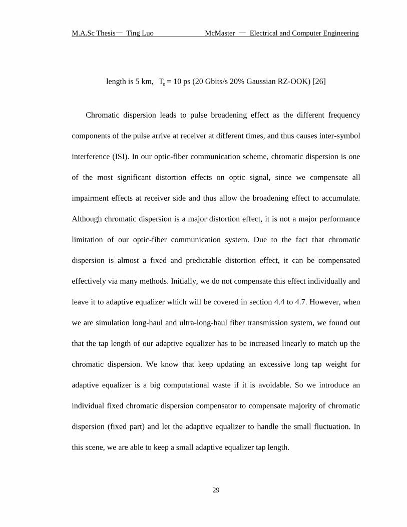
Figure 4.1: Illustration of a Gaussian pulses pass through a dispersive fiber, dispersion


29

length is 5 km, 0T = 10 ps (20 Gbits/s 20% Gaussian RZ-OOK) [26]

Chromatic dispersion leads to pulse broadening effect as the different frequency

components of the pulse arrive at receiver at different times, and thus causes inter-symbol

interference (ISI). In our optic-fiber communication scheme, chromatic dispersion is one

of the most significant distortion effects on optic signal, since we compensate all

impairment effects at receiver side and thus allow the broadening effect to accumulate.

Although chromatic dispersion is a major distortion effect, it is not a major performance

limitation of our optic-fiber communication system. Due to the fact that chromatic

dispersion is almost a fixed and predictable distortion effect, it can be compensated

effectively via many methods. Initially, we do not compensate this effect individually and

leave it to adaptive equalizer which will be covered in section 4.4 to 4.7. However, when

we are simulation long-haul and ultra-long-haul fiber transmission system, we found out

that the tap length of our adaptive equalizer has to be increased linearly to match up the

chromatic dispersion. We know that keep updating an excessive long tap weight for

adaptive equalizer is a big computational waste if it is avoidable. So we introduce an

individual fixed chromatic dispersion compensator to compensate majority of chromatic

dispersion (fixed part) and let the adaptive equalizer to handle the small fluctuation. In

this scene, we are able to keep a small adaptive equalizer tap length.


30

4.2 Fixed Chromatic Dispersion Compensator

A general long-haul fiber system will have a severe chromatic dispersion, resulting in

intensive inter-symbol interference (ISI). For example, a Gaussian pulse with T0= 10ps,

where T0 is the half-width at 1/e intensity point, travels through a 1000 km long fiber with

. At the end of fiber, this Gaussian pulse will be broadened 200 times

of the initial pules width. In order to compensate it, we need an equalizer, adaptive or

fixed, with at least 200 taps. Thus, with a fixed CD compensation, we do not have to

make our adaptive equalizer over 200 taps long. It will reduce the overall computation

cost dramatically due to the fact that a fixed tap weight do not need to be adjusted nor

updated at each iteration. By estimating the effective , we can introduce an inverse

dispersion to compensate the original dispersion just like dispersion compensating fiber

(DCF).

4.3 Polarization-Mode Dispersion Model

In our communication scheme, polarization-multiplexing QPSK (PM-QPSK),

polarization mode dispersion (PMD) is also an important distortion source that has to be

compensated properly. As we stated in section 1.2, compensating PMD requires an active

device that is able to self-adjust based on real time feedback, and the implementation of

such device in optical domain is very expansive and complex. However, the


31

implementation of such device in electrical domain is relatively much simpler and easier.

A tap and delay equalizer will able to handle it alone with many other distortion effects.

4.4 Adaptive Equalizer

Generally speaking, inter-symbol interference exists in all optical communication

system. A general tap and delay equalizer is the perfect device to compensate it and in

fact all linear distortion can be compensated. In most cases, we will operate optic-fiber

communication system in linear region where nonlinearity can be ignored. This is due to

the fact that the nonlinearity is hard to compensate while it comes and interacts with other

distortion effects and noises.

In a simple case where polarization multiplexing is not employed, PMD/PDL can be

neglected, and polarization alignment is done, we can illustrate the adaptive tap and delay

equalizer for this case in figure 4.2.

Figure 4.2 Structure map of a tap and delay equalizer with feedback.


32

[ ] [ ] [ ]

[ ] [ ] [ ]

[ ] { [ ] [ ] [ ] }

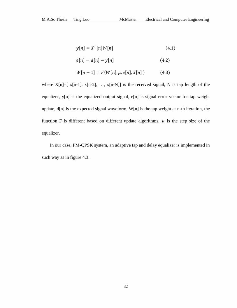
where X[n]=[ x[n-1], x[n-2], …, x[n-N]] is the received signal, N is tap length of the

equalizer, y[n] is the equalized output signal, e[n] is signal error vector for tap weight

update, d[n] is the expected signal waveform, W[n] is the tap weight at n-th iteration, the

function F is different based on different update algorithms, is the step size of the

equalizer.

In our case, PM-QPSK system, an adaptive tap and delay equalizer is implemented in

such way as in figure 4.3.


33

Xpol[n]

Ypol[n]

Xpol_o[n]

Ypol_o[n]

Figure 4.3 Block diagram of adaptive equalizer for coherent system.

Such scheme will also able to create an inverse jones matrix of fiber and thus able to

compensate cross-polarization interference. It will also able to handle any polarization

related distortion effect such as random polarization rotations.


34

4.5 System Overview

Figure 4.4 Block diagram of receiver layout using DSP compensation scheme

4.5.1 System with LMS adaptive equalizer

In our program, we implemented our DSP receiver according to figure 4.4. We

employ an ideal electrical filter right after the analog-digital converter (ADC) to reduce

total noise power. A fixed chromatic dispersion (CD) compensator is used after filter to

compensate bulk CD in long-haul communication system. It will remove majority of the

chromatic dispersion effect from signal and pass a relatively low distortion signal to

adaptive equalizer. The adaptive equalizer will then handle everything including

time-varying chromatic dispersion, laser phase noise, polarization- mode dispersion

(PMD), and other linear slow varying distortion effects. After equalizer, a phase noise

compensator is usually used to further tighten the signal from nearby constellation point.

However, phase noise compensator is not a must-have compensation device in the LMS

scheme since LMS adaptive equalizer also has the ability to handle phase noise and phase

rotation. In fact, via many different system simulations, we can conclude that if the LMS

Fiber Output Coherent Reciever Front End

ADC Digital Filter Fixed CD

Compensator Adaptive Equalizer

Phase Noise Compensator

Decision Device

DSP

Feedback


35

adaptive equalizer is optimized, a phase noise compensator is not necessary. In CMA

equalizer system, this statement is not valid, and we will cover this in more detail in

section 4.5.2. In optimal state, phase noise compensator may or may not improve system

bit error rate (BER) performance. Thus, phase noise compensator should be considered as

an optional device that ensures system performance when LMS adaptive equalizer

optimization is not guaranteed.

(a) (b)

(c) (d)

Figure 4.5 Constellation map of received signal at different LMS receiver stage.


36

Figure 4.5 (a) shows the signal constellation map after digital filter (before any

compensation). At this stage, the received signal is totally unreadable. Figure 4.5 (b)

shows the signal constellation map after fixed CD compensation. At this stage, major

chromatic dispersion effect has been removed and the signal becomes grouped and

somewhat distinguishable. Figure 4.5 (c) shows the signal constellation map after

adaptive Least Mean Square (LMS) equalizer. Most linear impairments have been

compensated now, and the signal is almost ready for detection. Figure 4.5 (d) shows the

signal constellation map after phase noise compensator. The signal constellation map is

more tightened and further away from nearby constellation point now. This will ensure

overall better system performance. Simulation parameters for figure 4.5: 30Gbit/s each

channel, PM-QPSK (4 channels), LMS adaptive equalizer used, launch power 0dbm,

transmitter and receiver laser line-width 1Mhz, ASE nsp=1.5, CD

, nonlinearity ⁄ , PMD Dp = 1 √ , lose

, 96k bits, , adaptive equalizer tap length =10, fiber length L =

10*115km. Figure 4.5 only shows the constellation maps for X polarization. Launch

power is the total power of two polarization signal unless otherwise stated.

After phase noise compensator (or adaptive equalizer if PN compensator is not

employed), signal is ready to pass through decision module. In decision module, signal

will be read based on maximum likelihood principle and the result will send back to


37

adaptive equalizer to generate reference signal d[n]. However, in our LMS algorithm, we

use soft decision result to generate reference signal d[n] instead of hard decision result

from output. Since the LMS algorithm is not capable of blind-detection, a training

sequence is required to train adaptive equalizer till the initial equalizer tap weight

converged. This training sequence is usually pre-defined and known. Receiver will use

this training sequence as desired signal d[n] in training stage. After a certain length of

training sequence have been applied (15k bits length in our program), the receiver change

to receiving stage and start using soft decision result to generate desired signal d[n].

4.5.2 System with CMA adaptive equalizer

Our CMA adaptive equalizer still follows the same receiver scheme described in

figure 4.4. As we mentioned in section 4.5.1, a phase noise compensator is no longer an

optional device in this scheme. Because CMA adaptive equalizer does not keep track on

current receiving bit and do not know the detail of default constellation point, it can only

restore the signal towards a QPSK scheme with a random rotation remained. A phase

noise compensator must be employed after CMA adaptive equalizer to remove this

random rotation (figure 4.6).


38

(a) (b)

(c) (d)

Figure 4.6 Constellation map of received signal at different CMA receiver stage.

Figure 4.6 (a) shows the signal constellation map after digital filter (before any

compensation). At this stage, the received signal is totally unreadable. Figure 4.6 (b)

shows the signal constellation map after fixed CD compensation. At this stage, major

chromatic dispersion effect has been removed and the signal becomes grouped and

somewhat distinguishable. Figure 4.6 (c) shows the signal constellation map after

adaptive CMA equalizer. The most linear impairments have been compensated, but the


39

signal is rotated randomly from default constellation point. Figure 4.6 (d) shows the

signal constellation map after phase noise compensator. The signal constellation map is

correctly rotated back to default constellation point now, and the signal is ready for

detection. Simulation parameters for figure 4.6: 30Gbit/s each channel, PM-QPSK (4

channels), launch power = -1dbm, transmitter and receiver laser line-width 1Mhz, ASE

nsp=1.5, CD , nonlinearity ⁄ , PMD Dp = 1

√ , lose , 96k bits, , adaptive equalizer tap length =10,

fiber length L = 10*115km. Figure 4.6 only shows the constellation maps for X

polarization.

4.6 Least Mean Square Adaptive Equalizer

Comparing to constant modulus algorithm (CMA), least mean square (LMS)

algorithms has many advantages including better stability, better performance, and faster

initialization speed. On the other hand, CMA is capable of blind detection and able to

self-recover in any case owing to its blind detection capability. There is no way to say one

is better than the other. It is just the matter of which one is best fit your need. We

implemented both solutions for our program.

As we discussed in section 4.4, a butterfly formation equalizer is used in our

PM-QPSK system. According to figure 4.3, we have


40

[ ] [ ] [ ]

[ ] [ ]

[ ] [ ] [ ]

[ ] [ ]

[ ] [ [ ] [ ]

[ ] [ ]]

[ ] 0

[ ]

[ ]

1

[ ] 0 [ ]

[ ]1

[ ] [ ] [ ]

Where , , , and are the tap weighs of adaptive equalizer, X[n] and

Y[n] is the input signal from x and y polarization, Xout[n] and Yout[n] is the compensated

signal output from equalizer. These formulas are true for both LMS and CMA adaptive

equalizer.

Specifically, LMS update its tap weigh according to equation 4.6 and 4.7.

[ ] 0

[ ]

[ ]

1

[ ] [ ] [ ]

[ ] [ ] [ ] [ ]

where d[n] is the reference signal, e[n] is the error vector.

A major disadvantage of LMS algorithm is that it requires a reference signal (desired

response) to compare with when updating its tap weigh. How should this reference signal


41

be generated is important to LMS algorithm. In our program, we employ two decision

devices for two purposes. The first one is the dedicated soft decision module which will

detect the estimated output signal of next bit, and then generate the desired response

d[n+1] based on the detection result. The adaptive equalizer will use this d [n+1] to

calculate new e[n+1] and [ ], and use the updated tap weigh to equalize I [n+1].

The result of them will now send to the second decision module (hard decision) for final

output. Similar to phase noise compensator, the separation of soft and hard decision is not

mandatory, and does not improve system performance dramatically.

4.6.1 Performance and optimization of LMS adaptive equalizer

Figure 4.7 BER vs. launch power optimization. Simulation parameters: 25Gbit/s each


42

channel, PM-QPSK (4 channels), launch power from -2dbm to 5dbm, transmitter and

receiver laser line-width 1Mhz, ASE nsp=1.5, CD , nonlinearity

⁄ , PMD Dp = 0.1 √ , lose , 96k bits, ,

adaptive equalizer tap length =10, fiber length L = 10*115km.

The center region in figure 4.7 (launch power from 0dbm to 3 dBm) is blank due to

the limitation of low simulation length which limits the minimum BER our simulation

program could obtain. In that power range, our simulations yield zero error and thus the

optimal launch power lies in that range. Because the BER is extremely low when

operating near optimal power range, our following simulation will be performed under

lower launch power.


43

Figure 4.8 BER vs. filter bandwidth ratio optimization. Simulation parameters: 25Gbit/s

each channel, PM-QPSK (4 channels), base bandwidth = 50Ghz, applied bandwidth =

base bandwidth * bandwidth ratio, launch power from -3dbm, transmitter and receiver

laser line-width 1Mhz, ASE nsp=1.5, CD , nonlinearity

⁄ , PMD Dp = 0.1 √ , lose , 96k bits, ,

adaptive equalizer tap length =10, fiber length L = 10*115km.

In this simulation, we notice that the filter bandwidth nearly does not affect out

system performance. In this case, we decided to set our bandwidth ratio to be 2 for future

simulation.

Figure 4.9 Pulse shape optimization. Simulation parameters: 25Gbit/s each channel,


44

PM-QPSK (4 channels), raised cosine pulse, applied bandwidth = base bandwidth *

bandwidth ratio, launch power from -3dbm, transmitter and receiver laser line-width

1Mhz, ASE nsp=1.5, CD , nonlinearity ⁄ , PMD

Dp = 0 ~ 1 √ , lose , 96k bits, , adaptive equalizer tap

length =10, fiber length L = 10*115km.

(a) (b)

Figure 4.10 Illustration of two pulse shapes. (a) alpha = 0.4, shaper (b) alpha = 0.8

smoother.

In this simulation, we not only found out that pulse shape (a) shown in figure 4.10

yields better performance, but also found out its interference with PMD. In our earlier

simulations, our simulation results always showed low PMD penalties. The lower the

PMD distortion effect the system has, the lower overall performance they system will

yield. This strange effect lead to this optimization which we found out that although

smoother pulse shape will reduce the signal bandwidth and should improve the


45

performance, it brings in another bigger problem that it lead to more ISI effect when

PMD exists. Thus, we choose figure 4.10 (a) pulse scheme for our simulations.

4.7 Constant Modulus Adaptive Equalizer

The major difference between CMA and LMS algorithm is how it updates the

adaptive equalizer tap weight. Due to the unique ability of CMA, CMA adaptive

equalizer does not need a desired signal (reference signal) to update itself which cause

CMA equalizer a blind-detection capable equalizer. The basic idea of CMA comes from

the nature of PSK system. All PSK constellation points have same modulus (distance

from origin) but different phase. Thus, CMA will calculate the cost (difference between

compensated signal modulus and standard modulus) of the current compensated signal,

and then update the tap weight to adapt the distortion effect. The blind-detection ability

comes from the fact that the CMA cost estimation does not rely on any signal

approximation but only the constant modulus, which is constant and specified in system

preset. CMA also natively only support PSK modulation scheme, but later advancement

also enable it to be used in some other modulation schemes like ASK by using complex

cost function. However, using PSK scheme can achieve the best CMA convergent rate

and stability.


46

[ ]

[ | [ ]|

| [ ]|

]

[ ] [ ] [ [ ]

[ ]]

[ ]

where cost[n] means the cost function of current sample, Mconstant means the standard

modulus of the system, [ ]* means complex conjugate, [ ]

T means transpose.

With the same system configuration, the optimization result of CMA equalizer is

generally the same as LMS. The detailed result will not present here for this reason.

4.8 Performance comparison of LMS and CMA

The following figure 4.11 shows a general system performance of LMS and CMA

adaptive equalizer. Generally, CMA has worse system performance than LMS algorithm

due to the fact that it does not keep track of current detection result even after system

converged. The blind-detection nature limits its compensation ability. However, the LMS

algorithm shows a nearly perfect system performance. Its performance almost overlapped

with ASE only case, meaning the LMS equalizer is almost able to compensate all linear

impairment effects. Another important advantage of LMS which is not shown in figure

4.11 is that the system stability. Once LMS equalizer have been optimized and converged,

it will almost never diverge again, and its maximum convergent time is limited and can be

calculated. However, the CMA doesn’t have such characteristic. The convergent time of


47

CMA generally decreased as the step size increased, but its stability also decreased

meanwhile.

Figure 4.11 Performance comparison of CMA and LMS adaptive equalizer. Simulation

parameters: 96k bits simulation length, 4 samples/symbol before ADC, 2 samples/symbol

after ADC, adaptive equalizer training length = 15k bits, 30G symbol/s per polarization

PM-QPSK system (120G bit/s total), laser line-width = 1MHz, number of WDM channels

= 1, 1550nm system, ASE nsp=1.5, CD , nonlinearity ⁄ ,

PMD Dp = 1 ps/(km-nm), lose , , adaptive equalizer tap length

=10, fiber length L = 10*115km. Note: CMA performance penalty also comes from

higher power nonlinearity effect which is not handled in receiver.

Chapter 5

Conclusion and Future Work


49

The laser frequency drift (laser phase noise), chromatic dispersion, and polarization

mode dispersion of the optical fiber could lead to performance degradation. In this thesis,

various electrical equalization techniques to mitigate these impairments are discussed.

In chapter 3, various techniques to compensate the laser phase noise are presented.

We discussed the M-th power method, unwarping algorithm, and update step size control

technique used in phase noise compensation module. Performance comparison of

different system configurations is also given in the end. We concluded that the block

phase noise compensation scheme with a block size of 10 and phase update limit enforced

is the best of all. We used this scheme in our following simulations.

In chapter 4, we discussed the implementation of both LMS and CMA adaptive

equalizer solution, and the corresponding phase noise compensator for both equalizers.

Although wavelength-division multiplexing (WDM) is not discussed in this thesis, such

system configuration is also supported in this tool. With this simulation tool, we are able

to compare the performance of many different system configurations, and examine the

impact of a specify system parameter change. Also, we are able to prove the performance

of DSP compensation device in varies situations.

Our results show that the DSP compensation scheme in coherent polarization

multiplexing QPSK is very effective in compensating linear distortion effects. The LMS

adaptive equalizer scheme has almost perfect compensating capability, while the CMA


50

adaptive equalizer scheme has bind-detection ability. Although the current version

simulation tool does not have the ability to use LMS and CMA adaptive equalizer

together, it still would be a very good future work direction. Combining the LMS and

CMA algorithm together, by using CMA in training stage and LMS in receiving stage,

might combine the advantage of both algorithms together. It will give such DSP receiver

not only the bind initialization and the capability to automatically recover from errors

from CMA, but also the near perfect compensation performance and stability from LMS.

Finally, there are still many directions we can improve our equalization techniques

such as experimental validation, additional function and mode support, and/or improved

simulation speed.


51

Bibliography [1] J. I. Yamada, S. Machida and T. Kimura, “2 Gbit/s optical transmission experiments

at 1.3 with 44 km single-mode fibre,” Electron. Lett. 17, 479 (1981).

[2] G. P. Agrawal, Fiber-Optic Communication Systems (John Wiley & Sons, New York,

2002).

[3] M. G. Taylor, "Coherent detection method using DSP to demodulate signal and

subsequent equalization of propagation impairments", European Conference on Optical

Communications, paper We4.P.111, Rimini, Italy, Sept. 2003.

[4] S. A. Tretter, “Estimating the Frequency of a Noisy Sinusoid by Linear Regression”

IEEE Transactions on Information Theory, vol. it-31, no. 6, pp. 832-835, Nov 1985.

[5] S. Kay, “A fast and Accurate Single Frequency Estimator” IEEE Transactions on

Acoustics Speech and Signal Processing, vol. 37, No. 12, pp. 1987-1990, Dec 1989.

[6] E. Ip and M. Kahn, “Feedforward carrier recovery for coherent optical

communications” J. Lightwave Technology, vol. 25, no. 9, pp. 2675-2692, Sep 2007.

[7] D. E. Crivelli, H. S. Carter, and M. R. Hueda, “Adaptive digital equalization in the

presence of chromatic dispersion, PMD, and phase noise in coherent fiber optic systems”

IEE Global Telecommunication Conference (GLOBECOM), Dallas, TX, 2004, vol. 4, pp.

2545-2551.

[8] A. Viterbi and A. Viterbi, “Nonlinear estimation of PSK-modulated carrier phase with


52

application to burst digital transmission” IEEE transactions on information theory, vol.

IT-29, no. 4, July 1983.

[9] D.-S. Ly-Gagnon, S. Tsukamoto, K. Katoh, and K. Kikuchi, “ Coherent detection of

optical quadrature phase shift keying signals with carrier phase estimation” J. Lightwave

Technology, vol. 24, no. 1, pp. 12-21, Jan. 2006.

[10] M. G. Taylor, “Accurate digital phase estimation process for coherent detection

using a parallel digital processor,” European Conference on Optical Communications,

paper Tu4.2.6, Glasgow, Scotland, Sep. 2005.

[11] S. Tsukamoto, K. Katoh, and K. Kikuchi, “Unrepeated transmission of 20 Gb/s

optical quadrature phase shift keying signal over 200 km standard single mode fiber

based on digital processing of homodyne detected signal for group velocity dispersion

compensation” IEEE Photon Technology Lett., vol. 18, no. 9, pp. 1016-1018, May 2006.

[12] E. Ip and M. Kahn, “Digital equalization of chromatic dispersion and polarization

mode dispersion” J. Lightwave Technology, vol. 25, no. 8, pp. 2033-2043, Aug. 2007.

[13] C. S. Fludger, T. Duthel, T. Wuth, and C. Schulien, “ Uncompensated transmission

of 86 Gbps polarization multiplexed RZ-QPSK over 100 km of NDSF employing

coherent equalization” European Conference on Optical Communications, paper Th4.3.3,

Cannes, France, Sep. 2006.

[14]A. Leven, N. Kaneda, Y. K. Chen, “A real-time CMA-based 10 Gb/s polarization


53

demultiplexing coherent receiver implemented in an FPGA” Optical Fiber

Communication Conference, paper OTuO2, San Diego, CA, Feb. 2008.

[15] C. S. Fludger, T. Duthel, D. van den Borne, C. Schulien, E. D. Schmidt, T. Wuth, J.

Geyer, E. D. Man, G. D. Khoe and H. de Waart, “Digital equalization of chromatic

dispersion and polarization mode dispersion” J. Lightwave Technology, vol. 28, no. 11,

pp. 1867-1875, Nov. 1980.

[16] D. Godard, “Self-recovering equalization and carrier tracking in two dimensional

data communication systems” IEE Transcation communication, vol. 28, no. 11, pp.

1867-1875, Nov. 1980.

[17] C. R. Johnson, P. Schniter, T. J. Endres, J. D. Behm, D. R. Brown, and R. A. Casas,

“Blind Equalization Using the Constant Modulus Criterion: A Review” Proceedings of

the IEEE, vol. 86, no. 10, Oct. 1998.

[18] C. Laperle, B. Villeneuve, Z. Zhan, D. McGhan, H. Sun, and M. O. Sullivan, “WDM

performance and PMD tolerance of a coherent 40 Gbit/s Dual-Polarization QPSK

Transceiver” J. Lightwave Technology, vol. 26, no. 1 pp. 168-175, Jan. 2008.

[19] S. J. Savory, G. Gavioli, R. I. Killey, and P. Bayvel, “ Electronic compensation of

chromatic dispersion using a digital coherent receiver” Optics Express, vol. 18, no. 5, pp.

2120-2126, Mar. 2007.

[20] J. Renaudier, G. Charlet, M. Salsi, O. B. Pardo, H. Mardoyan, P. Tran and S. Bigo,


54

“Linear fiber impairment mitigation of 40 Gbit/s polarization mulitiplexed QPSK by

digital processing in coherent receiver” J. Lightwave Technology, vol. 26, no. 1, pp.

36-42, Jan. 2008.

[21] M. Morelli and U. Mengali, “Feedforward Frequency Estimation for PSK: a Tutorial

Review,” European Trans. on Telecommunication, Vol. 2, pp.103-116, March/April 1998

[22] E. Ip and M. Kahn, “Feedforward carrier recovery for coherent optical

communications,” J. Lightwave Technology, Vol. 25, no. 9, pp.2684-2692, Sep. 2007

[23] M. G. Taylor, “Accurate digital phase estimation process for coherent detection

using a parallel digital processor,” European Conference on Optical Communications,

paper Tu4.2.6, Glasgow, Scotland, Sep. 2005

[24] A. Viterbi and A. Viterbi, “nonlinear estimation of PSK-modulated carrier phase

with application to burst digital transmission,” IEEE Trans, on Information Theory, vol.

IT-29, oo.4, July 1983.

[25] D.-S. Ly-Gagnon, S. Tsukamoto, K. Katoh, and K. Kikuchi, “Coherent detection of

optical quadrature phase-shift keying signals wiwth carrier phase estimation,” J.

Lightwave. Technology, vol. 24, no. 1, pp. 12-21, Jan. 2006

[26] X. Deng, “A modified split-step Fourier scheme for fiber-optic communication

system and its application to forward and backward propagation”, McMaster University,

2010.


55

[27] Govind P. Agrawal “Fiber-Optic Communication Systems” Wiley-Interscience, third

edition, 2002.

C.S Petrou, A. Vgenis, I. Roudas, J. Hurley, M. Sauer, J. Downie, Y. Mauro, and S.

Raghavan “Experimental testing of DSP algorithms for digital intradyne coherent QPSK

phase- and polarization-diversity receivers” 2010

Digital Equalization of Fiber-Optic Transmission System ... · PDF fileiii Abstract In the...

Documents

Transcript of Digital Equalization of Fiber-Optic Transmission System ... · PDF fileiii Abstract In the...