Digital Communication Systems - The Free Information Society

Digital Communication Systems

By:Behnaam Aazhang

Digital Communication Systems

By:Behnaam Aazhang

Online:<http://cnx.org/content/col10134/1.3/ >

C O N N E X I O N S

Rice University, Houston, Texas

©2008 Behnaam Aazhang

This selection and arrangement of content is licensed under the Creative Commons Attribution License:

http://creativecommons.org/licenses/by/1.0

Table of Contents

1 Chapter 1

2 Chapter 2

2.1 Review of Probability Theory . . . . . . . . . . . . . . . . . . . . . . . . . . . . . . . . . . . . . . . . . . . . . . . . . . . . . . . . . . . . . . . . 3

3 Chapter 3

3.1 Introduction to Stochastic Processes . . . . . . . . . . . . . . . . . . . . . . . . . . . . . . . . . . . . . . . . . . . . . . . . . . . . . . . . . 73.2 Second-order Description . . . . . . . . . . . . . . . . . . . . . . . . . . . . . . . . . . . . . . . . . . . . . . . . . . . . . . . . . . . . . . . . . . . 113.3 Linear Filtering . . . . . . . . . . . . . . . . . . . . . . . . . . . . . . . . . . . . . . . . . . . . . . . . . . . . . . . . . . . . . . . . . . . . . . . . . . . . .133.4 Gaussian Processes . . . . . . . . . . . . . . . . . . . . . . . . . . . . . . . . . . . . . . . . . . . . . . . . . . . . . . . . . . . . . . . . . . . . . . . . . 16

4 Chapter 4

4.1 Data Transmission and Reception . . . . . . . . . . . . . . . . . . . . . . . . . . . . . . . . . . . . . . . . . . . . . . . . . . . . . . . . . . .174.2 Signalling . . . . . . . . . . . . . . . . . . . . . . . . . . . . . . . . . . . . . . . . . . . . . . . . . . . . . . . . . . . . . . . . . . . . . . . . . . . . . . . . . . .174.3 Geometric Representation of Modulation Signals . . . . . . . . . . . . . . . . . . . . . . . . . . . . . . . . . . . . . . . . . . . . 214.4 Demodulation and Detection . . . . . . . . . . . . . . . . . . . . . . . . . . . . . . . . . . . . . . . . . . . . . . . . . . . . . . . . . . . . . . . 244.5 Demodulation . . . . . . . . . . . . . . . . . . . . . . . . . . . . . . . . . . . . . . . . . . . . . . . . . . . . . . . . . . . . . . . . . . . . . . . . . . . . . . 254.6 Detection by Correlation . . . . . . . . . . . . . . . . . . . . . . . . . . . . . . . . . . . . . . . . . . . . . . . . . . . . . . . . . . . . . . . . . . . 284.7 Examples of Correlation Detection . . . . . . . . . . . . . . . . . . . . . . . . . . . . . . . . . . . . . . . . . . . . . . . . . . . . . . . . . . 304.8 Matched Filters . . . . . . . . . . . . . . . . . . . . . . . . . . . . . . . . . . . . . . . . . . . . . . . . . . . . . . . . . . . . . . . . . . . . . . . . . . . . 324.9 Examples with Matched Filters . . . . . . . . . . . . . . . . . . . . . . . . . . . . . . . . . . . . . . . . . . . . . . . . . . . . . . . . . . . . . 344.10 Matched Filters in the Frequency Domain . . . . . . . . . . . . . . . . . . . . . . . . . . . . . . . . . . . . . . . . . . . . . . . . . 364.11 Performance Analysis . . . . . . . . . . . . . . . . . . . . . . . . . . . . . . . . . . . . . . . . . . . . . . . . . . . . . . . . . . . . . . . . . . . . . 384.12 Performance Analysis of Antipodal Binary signals with Correlation . . . . . . . . . . . . . . . . . . . . . . . . 384.13 Performance Analysis of Binary Orthogonal Signals with Correlation . . . . . . . . . . . . . . . . . . . . . . 394.14 Performance Analysis of Binary Antipodal Signals with Matched Filters . . . . . . . . . . . . . . . . . . . 414.15 Performance Analysis of Orthogonal Binary Signals with Matched Filters . . . . . . . . . . . . . . . . . . 42

5 Chapter 5

5.1 Digital Transmission over Baseband Channels . . . . . . . . . . . . . . . . . . . . . . . . . . . . . . . . . . . . . . . . . . . . . . .455.2 Pulse Amplitude Modulation Through Bandlimited Channel . . . . . . . . . . . . . . . . . . . . . . . . . . . . . . . . 455.3 Precoding and Bandlimited Signals . . . . . . . . . . . . . . . . . . . . . . . . . . . . . . . . . . . . . . . . . . . . . . . . . . . . . . . . . 46

6 Chapter 6

6.1 Carrier Phase Modulation . . . . . . . . . . . . . . . . . . . . . . . . . . . . . . . . . . . . . . . . . . . . . . . . . . . . . . . . . . . . . . . . . . 496.2 Dierential Phase Shift Keying . . . . . . . . . . . . . . . . . . . . . . . . . . . . . . . . . . . . . . . . . . . . . . . . . . . . . . . . . . . . . 516.3 Carrier Frequency Modulation . . . . . . . . . . . . . . . . . . . . . . . . . . . . . . . . . . . . . . . . . . . . . . . . . . . . . . . . . . . . . . 52

7 Chapter 7

7.1 Information Theory and Coding . . . . . . . . . . . . . . . . . . . . . . . . . . . . . . . . . . . . . . . . . . . . . . . . . . . . . . . . . . . . 557.2 Entropy . . . . . . . . . . . . . . . . . . . . . . . . . . . . . . . . . . . . . . . . . . . . . . . . . . . . . . . . . . . . . . . . . . . . . . . . . . . . . . . . . . . . 567.3 Source Coding . . . . . . . . . . . . . . . . . . . . . . . . . . . . . . . . . . . . . . . . . . . . . . . . . . . . . . . . . . . . . . . . . . . . . . . . . . . . . . 597.4 Human Coding . . . . . . . . . . . . . . . . . . . . . . . . . . . . . . . . . . . . . . . . . . . . . . . . . . . . . . . . . . . . . . . . . . . . . . . . . . . . 627.5 Channel Capacity . . . . . . . . . . . . . . . . . . . . . . . . . . . . . . . . . . . . . . . . . . . . . . . . . . . . . . . . . . . . . . . . . . . . . . . . . . 637.6 Mutual Information . . . . . . . . . . . . . . . . . . . . . . . . . . . . . . . . . . . . . . . . . . . . . . . . . . . . . . . . . . . . . . . . . . . . . . . . 657.7 Typical Sequences . . . . . . . . . . . . . . . . . . . . . . . . . . . . . . . . . . . . . . . . . . . . . . . . . . . . . . . . . . . . . . . . . . . . . . . . . . 677.8 Shannon's Noisy Channel Coding Theorem . . . . . . . . . . . . . . . . . . . . . . . . . . . . . . . . . . . . . . . . . . . . . . . . . 697.9 Channel Coding . . . . . . . . . . . . . . . . . . . . . . . . . . . . . . . . . . . . . . . . . . . . . . . . . . . . . . . . . . . . . . . . . . . . . . . . . . . . 717.10 Convolutional Codes . . . . . . . . . . . . . . . . . . . . . . . . . . . . . . . . . . . . . . . . . . . . . . . . . . . . . . . . . . . . . . . . . . . . . . 74Solutions . . . . . . . . . . . . . . . . . . . . . . . . . . . . . . . . . . . . . . . . . . . . . . . . . . . . . . . . . . . . . . . . . . . . . . . . . . . . . . . . . . . . . . . . 76

8 Homework

iv

9 Homework 1 of Elec 430 . . . . . . . . . . . . . . . . . . . . . . . . . . . . . . . . . . . . . . . . . . . . . . . . . . . . . . . . . . . . . . . . . . . . . . . . . 7910 Homework 2 of Elec 430 . . . . . . . . . . . . . . . . . . . . . . . . . . . . . . . . . . . . . . . . . . . . . . . . . . . . . . . . . . . . . . . . . . . . . . . .8111 Homework 5 of Elec 430 . . . . . . . . . . . . . . . . . . . . . . . . . . . . . . . . . . . . . . . . . . . . . . . . . . . . . . . . . . . . . . . . . . . . . . . .8312 Homework 3 of Elec 430 . . . . . . . . . . . . . . . . . . . . . . . . . . . . . . . . . . . . . . . . . . . . . . . . . . . . . . . . . . . . . . . . . . . . . . . .8713 Exercises on Systems and Density . . . . . . . . . . . . . . . . . . . . . . . . . . . . . . . . . . . . . . . . . . . . . . . . . . . . . . . . . . . . .8914 Homework 6 . . . . . . . . . . . . . . . . . . . . . . . . . . . . . . . . . . . . . . . . . . . . . . . . . . . . . . . . . . . . . . . . . . . . . . . . . . . . . . . . . . . . . 9115 Homework 7 . . . . . . . . . . . . . . . . . . . . . . . . . . . . . . . . . . . . . . . . . . . . . . . . . . . . . . . . . . . . . . . . . . . . . . . . . . . . . . . . . . . . . 9516 Homework 8 . . . . . . . . . . . . . . . . . . . . . . . . . . . . . . . . . . . . . . . . . . . . . . . . . . . . . . . . . . . . . . . . . . . . . . . . . . . . . . . . . . . . . 9717 Homework 9 . . . . . . . . . . . . . . . . . . . . . . . . . . . . . . . . . . . . . . . . . . . . . . . . . . . . . . . . . . . . . . . . . . . . . . . . . . . . . . . . . . . . . 99Glossary . . . . . . . . . . . . . . . . . . . . . . . . . . . . . . . . . . . . . . . . . . . . . . . . . . . . . . . . . . . . . . . . . . . . . . . . . . . . . . . . . . . . . . . . . . . . 100Index . . . . . . . . . . . . . . . . . . . . . . . . . . . . . . . . . . . . . . . . . . . . . . . . . . . . . . . . . . . . . . . . . . . . . . . . . . . . . . . . . . . . . . . . . . . . . . . 104Attributions . . . . . . . . . . . . . . . . . . . . . . . . . . . . . . . . . . . . . . . . . . . . . . . . . . . . . . . . . . . . . . . . . . . . . . . . . . . . . . . . . . . . . . . .106

Chapter 1

Chapter 1

1

2 CHAPTER 1. CHAPTER 1

Chapter 2

Chapter 2

2.1 Review of Probability Theory1

The focus of this course is on digital communication, which involves transmission of information, in itsmost general sense, from source to destination using digital technology. Engineering such a system requiresmodeling both the information and the transmission media. Interestingly, modeling both digital or analoginformation and many physical media requires a probabilistic setting. In this chapter and in the next one wewill review the theory of probability, model random signals, and characterize their behavior as they traversethrough deterministic systems disturbed by noise and interference. In order to develop practical models forrandom phenomena we start with carrying out a random experiment. We then introduce denitions, rules,and axioms for modeling within the context of the experiment. The outcome of a random experiment isdenoted by ω. The sample space Ω is the set of all possible outcomes of a random experiment. Such outcomescould be an abstract description in words. A scientic experiment should indeed be repeatable where eachoutcome could naturally have an associated probability of occurrence. This is dened formally as the ratioof the number of times the outcome occurs to the total number of times the experiment is repeated.

2.1.1 Random Variables

A random variable is the assignment of a real number to each outcome of a random experiment.

Figure 2.1

Example 2.1Roll a dice. Outcomes ω1, ω2, ω3, ω4, ω5, ω6

1This content is available online at <http://cnx.org/content/m10224/2.16/>.

3


ωi = i dots on the face of the dice.X (ωi) = i

2.1.2 Distributions

Probability assignments on intervals a < X ≤ b

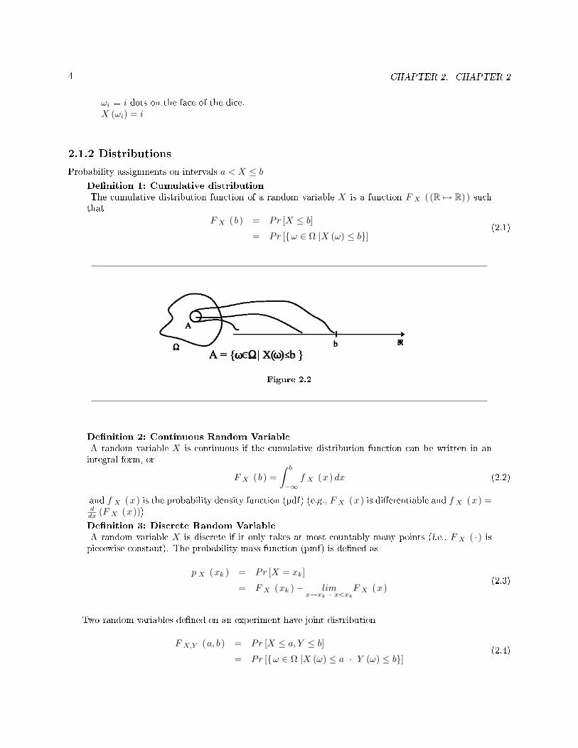
Denition 1: Cumulative distributionThe cumulative distribution function of a random variable X is a function F X ( (R 7→ R) ) suchthat

F X (b ) = Pr [X ≤ b]

= Pr [ω ∈ Ω |X (ω) ≤ b](2.1)

Figure 2.2

Denition 2: Continuous Random VariableA random variable X is continuous if the cumulative distribution function can be written in anintegral form, or

F X (b ) =∫ b

−∞f X (x ) dx (2.2)

and f X (x ) is the probability density function (pdf) (e.g., F X (x ) is dierentiable and f X (x ) =ddx (F X (x )))Denition 3: Discrete Random VariableA random variable X is discrete if it only takes at most countably many points (i.e., F X ( · ) ispiecewise constant). The probability mass function (pmf) is dened as

p X (xk ) = Pr [X = xk]

= F X (xk )− limx→xk · x<xk

F X (x )(2.3)

Two random variables dened on an experiment have joint distribution

F X,Y (a, b ) = Pr [X ≤ a, Y ≤ b]

= Pr [ω ∈ Ω |X (ω) ≤ a · Y (ω) ≤ b](2.4)

5

Figure 2.3

Joint pdf can be obtained if they are jointly continuous

F X,Y (a, b ) =∫ b

−∞

∫ a

−∞f X,Y (x, y ) dxdy (2.5)

(e.g., f X,Y (x, y ) = ∂2

∂x∂y (F X,Y (x, y )))Joint pmf if they are jointly discrete

p X,Y (xk, yl ) = Pr [X = xk, Y = yl] (2.6)

Conditional density function

fY |X (y|x) =f X,Y (x, y )f X (x )

(2.7)

for all x with f X (x ) > 0 otherwise conditional density is not dened for those values of x with f X (x ) = 0Two random variables are independent if

f X,Y (x, y ) = f X (x ) f Y (y ) (2.8)

for all x ∈ R and y ∈ R. For discrete random variables,

p X,Y (xk, yl ) = p X (xk ) p Y (yl ) (2.9)

for all k and l.

2.1.3 Moments

Statistical quantities to represent some of the characteristics of a random variable.

g (X) = E [g (X)]

=

∫∞−∞ g (x) f X (x ) dx if continuous∑

k (g (xk) p X (xk )) if discrete

(2.10)


• MeanµX = X (2.11)

• Second momentE[X2]

= X2 (2.12)

• Variance

V ar (X) = σ(X)2

= (X − µX)2

= X2 − µX2

(2.13)

• Characteristic functionΦX (u) = ejuX (2.14)

for u ∈ R, where j =√−1

• Correlation between two random variables

RXY = XY ∗

=

∫∞−∞

∫∞−∞ xy∗f X,Y (x, y ) dxdy if X and Y are jointly continuous∑

k (∑

l (xky∗l p X,Y (xk, yl ))) if X and Y are jointly discrete

(2.15)

• Covariance

CXY = Cov (X,Y )

= (X − µX) (Y − µY )∗

= RXY − µXµ∗Y

(2.16)

• Correlation coecient

ρXY =Cov (X,Y )σXσY

(2.17)

Denition 4: Uncorrelated random variablesTwo random variables X and Y are uncorrelated if ρXY = 0.

Chapter 3

Chapter 3

3.1 Introduction to Stochastic Processes1

3.1.1 Denitions, distributions, and stationarity

Denition 5: Stochastic ProcessGiven a sample space, a stochastic process is an indexed collection of random variables dened foreach ω ∈ Ω.

Xt (ω) , t ∈ R (3.1)

Example 3.1Received signal at an antenna as in Figure 3.1.

Figure 3.1


7


For a given t, Xt (ω) is a random variable with a distribution

First-order distribution

FXt (b) = Pr [Xt ≤ b]

= Pr [ω ∈ Ω |Xt (ω) ≤ b](3.2)

Denition 6: First-order stationary processIf FXt (b) is not a function of time then Xt is called a rst-order stationary process.

Second-order distribution

FXt1 ,Xt2(b1, b2) = Pr [Xt1 ≤ b1, Xt2 ≤ b2] (3.3)

for all t1 ∈ R, t2 ∈ R, b1 ∈ R, b2 ∈ RNth-order distribution

FXt1 ,Xt2 ,...,XtN(b1, b2, . . . , bN ) = Pr [Xt1 ≤ b1, . . . , XtN

≤ bN ] (3.4)

Nth-order stationary : A random process is stationary of order N if

FXt1 ,Xt2 ,...,XtN(b1, b2, . . . , bN ) = FXt1+T ,Xt2+T ,...,XtN +T

(b1, b2, . . . , bN ) (3.5)

Strictly stationary : A process is strictly stationary if it is Nth order stationary for all N .

Example 3.2Xt = cos (2πf0t+ Θ(ω)) where f0 is the deterministic carrier frequency and Θ(ω) : (Ω → R)is a random variable dened over [−π, π] and is assumed to be a uniform random variable; i.e.,

fΘ (θ) =

12π if θ ∈ [−π, π]

0 otherwise

FXt (b) = Pr [Xt ≤ b]

= Pr [cos (2πf0t+ Θ) ≤ b](3.6)

FXt (b) = Pr [−π ≤ 2πf0t+ Θ ≤ − (arccos (b))] + Pr [arccos (b) ≤ 2πf0t+ Θ ≤ π] (3.7)

FXt (b) =∫ −(arccos(b))−2πf0t

−π−2πf0t12πdθ +

∫ π−2πf0t

arccos(b)−2πf0t12πdθ

= (2π − 2arccos (b)) 12π

(3.8)

fXt (x) = ddx

(1− 1

πarccos (x))

=

1π√

1−x2 if |x| ≤ 1

0 otherwise

(3.9)

This process is stationary of order 1.

9

Figure 3.2

The second order stationarity can be determined by rst considering conditional densities andthe joint density. Recall that

Xt = cos (2πf0t+ Θ) (3.10)

Then the relevant step is to nd

Pr [Xt2 ≤ b2 | Xt1 = x1] (3.11)

Note thatXt1 = x1 = cos (2πf0t+ Θ) ⇒ Θ = arccos (x1)− 2πf0t (3.12)

Xt2 = cos (2πf0t2 + arccos (x1)− 2πf0t1)

= cos (2πf0 (t2 − t1) + arccos (x1))(3.13)

Figure 3.3


FXt2 ,Xt1(b2, b1) =

∫ b1

−∞fXt1

(x1)Pr [Xt2 ≤ b2 | Xt1 = x1] dx1 (3.14)

Note that this is only a function of t2 − t1.

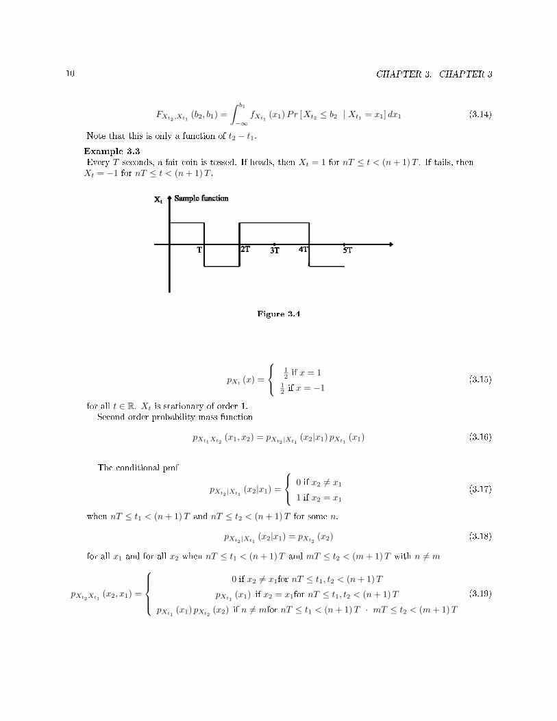
Example 3.3Every T seconds, a fair coin is tossed. If heads, then Xt = 1 for nT ≤ t < (n+ 1)T . If tails, thenXt = −1 for nT ≤ t < (n+ 1)T .

Figure 3.4

pXt(x) =

12 if x = 1

12 if x = −1

(3.15)

for all t ∈ R. Xt is stationary of order 1.Second order probability mass function

pXt1Xt2(x1, x2) = pXt2 |Xt1

(x2|x1) pXt1(x1) (3.16)

The conditional pmf

pXt2 |Xt1(x2|x1) =

0 if x2 6= x1

1 if x2 = x1

(3.17)

when nT ≤ t1 < (n+ 1)T and nT ≤ t2 < (n+ 1)T for some n.

pXt2 |Xt1(x2|x1) = pXt2

(x2) (3.18)

for all x1 and for all x2 when nT ≤ t1 < (n+ 1)T and mT ≤ t2 < (m+ 1)T with n 6= m

pXt2Xt1(x2, x1) =

0 if x2 6= x1for nT ≤ t1, t2 < (n+ 1)T

pXt1(x1) if x2 = x1for nT ≤ t1, t2 < (n+ 1)T

pXt1(x1) pXt2

(x2) if n 6= mfor nT ≤ t1 < (n+ 1)T · mT ≤ t2 < (m+ 1)T

(3.19)

11

3.2 Second-order Description2

3.2.1 Second-order description

Practical and incomplete statistics

Denition 7: MeanThe mean function of a random process Xt is dened as the expected value of Xt for all t's.

µXt= E [Xt]

=

∫∞−∞ xf Xt (x ) dx if continuous∑∞k=−∞ (xkp Xt

(xk )) if discrete

(3.20)

Denition 8: AutocorrelationThe autocorrelation function of the random process Xt is dened as

RX (t2, t1) = E [Xt2Xt1∗]

=

∫∞−∞

∫∞−∞ x2x1

∗f Xt2 ,Xt1(x2, x1 ) dx1dx2 if continuous∑∞

k=−∞(∑∞

l=−∞(xlxk

∗p Xt2 ,Xt1(xl, xk )

))if discrete

(3.21)

Fact 3.1:If Xt is second-order stationary, then RX (t2, t1) only depends on t2 − t1.Proof:

RX (t2, t1) = E [Xt2Xt1∗]

=∫∞−∞

∫∞−∞ x2x1

∗f Xt2 ,Xt1(x2, x1 ) dx2dx1

(3.22)

RX (t2, t1) =∫∞−∞

∫∞−∞ x2x1

∗f Xt2−t1 ,X0 (x2, x1 ) dx2dx1

= RX (t2 − t1, 0)(3.23)

If RX (t2, t1) depends on t2 − t1 only, then we will represent the autocorrelation with only one variableτ = t2 − t1

RX (τ) = RX (t2 − t1)

= RX (t2, t1)(3.24)

Properties

1. RX (0) ≥ 02. RX (τ) = RX (−τ)∗3. |RX (τ) | ≤ RX (0)

Example 3.4Xt = cos (2πf0t+ Θ(ω)) and Θ is uniformly distributed between 0 and 2π. The mean function

µX (t) = E [Xt]

= E [cos (2πf0t+ Θ)]

=∫ 2π

0cos (2πf0t+ θ) 1

2πdθ

= 0

(3.25)



The autocorrelation function

RX (t+ τ, t) = E [Xt+τXt∗]

= E [cos (2πf0 (t+ τ) + Θ) cos (2πf0t+ Θ)]

= 1/2E [cos (2πf0τ)] + 1/2E [cos (2πf0 (2t+ τ) + 2Θ)]

= 1/2cos (2πf0τ) + 1/2∫ 2π

0cos (2πf0 (2t+ τ) + 2θ) 1

2πdθ

= 1/2cos (2πf0τ)

(3.26)

Not a function of t since the second term in the right hand side of the equality in (3.26) is zero.

Example 3.5Toss a fair coin every T seconds. Since Xt is a discrete valued random process, the statisticalcharacteristics can be captured by the pmf and the mean function is written as

µX (t) = E [Xt]

= 1/2× (−1) + 1/2× 1

= 0

(3.27)

RX (t2, t1) =∑

k

(∑l

(xkxlp Xt2 ,Xt1

(xk, xl )))

= 1× 1× 1/2 + (−1×−1× 1/2)

= 1

(3.28)

when nT ≤ t1 < (n+ 1)T and nT ≤ t2 < (n+ 1)T

RX (t2, t1) = 1× 1× 1/4 + (−1×−1× 1/4) + (−1× 1× 1/4) + 1×−1× 1/4

= 0(3.29)

when nT ≤ t1 < (n+ 1)T and mT ≤ t2 < (m+ 1)T with n 6= m

RX (t2, t1) =

1 if nT ≤ t1 < (n+ 1)T · nT ≤ t2 < (n+ 1)T

0 otherwise(3.30)

A function of t1 and t2.

Denition 9: Wide Sense StationaryA process is said to be wide sense stationary if µX is constant and RX (t2, t1) is only a function oft2 − t1.

Fact 3.1:If Xt is strictly stationary, then it is wide sense stationary. The converse is not necessarily true.

Denition 10: AutocovarianceAutocovariance of a random process is dened as

CX (t2, t1) = E[(Xt2 − µX (t2))Xt1 − µX (t1)

∗]= RX (t2, t1)− µX (t2)µX (t1)

∗ (3.31)

The variance of Xt is V ar (Xt) = CX (t, t)Two processes dened on one experiment (Figure 3.5).

13

Figure 3.5

Denition 11: CrosscorrelationThe crosscorrelation function of a pair of random processes is dened as

RXY (t2, t1) = E [Xt2Yt1∗]

=∫∞−∞

∫∞−∞ xyf Xt2 ,Yt1

(x, y ) dxdy(3.32)

CXY (t2, t1) = RXY (t2, t1)− µX (t2)µY (t1)∗

(3.33)

Denition 12: Jointly Wide Sense StationaryThe random processes Xt and Yt are said to be jointly wide sense stationary if RXY (t2, t1) is afunction of t2 − t1 only and µX (t) and µY (t) are constant.

3.3 Linear Filtering3

Integration

Z (ω) =∫ b

a

Xt (ω) dt (3.34)

Linear Processing

Yt =∫ ∞

−∞h (t, τ)Xτdτ (3.35)

Dierentiation

Xt′ =

d

dt(Xt) (3.36)

Properties

1. Z =∫ b

aXt (ω) dt =

∫ b

aµX (t) dt

2. Z2 =∫ b

aXt2dt2

∫ b

aXt1

∗dt1 =∫ b

a

∫ b

aRX (t2, t1) dt1dt2



Figure 3.6

µY (t) =∫∞−∞ h (t, τ)Xτdτ

=∫∞−∞ h (t, τ)µX (τ) dτ

(3.37)

If Xt is wide sense stationary and the linear system is time invariant

µY (t) =∫∞−∞ h (t− τ)µXdτ

= µX

∫∞−∞ h (t′) dt′

= µY

(3.38)

RY X (t2, t1) = Yt2Xt1∗

=∫∞−∞ h (t2 − τ)XτdτXt1

∗

=∫∞−∞ h (t2 − τ)RX (τ − t1) dτ

(3.39)

RY X (t2, t1) =∫∞−∞ h (t2 − t1 − τ ′)RX (τ ′) dτ ′

= h ∗RX (t2 − t1)(3.40)

where τ ′ = τ − t1.

RY (t2, t1) = Yt2Yt1∗

= Yt2

∫∞−∞ h (t1, τ)Xτ

∗dτ

=∫∞−∞ h (t1, τ)RY X (t2, τ) dτ

=∫∞−∞ h (t1 − τ)RY X (t2 − τ) dτ

(3.41)

RY (t2, t1) =∫∞−∞ h (τ ′ − (t2 − t1))RY X (τ ′) dτ ′

= RY (t2 − t1)

=∼h ∗RY X (t2, t1)

(3.42)

where τ ′ = t2 − τ and∼h (τ) = h (−τ) for all τ ∈ R. Yt is WSS if Xt is WSS and the linear system is

time-invariant.

15

Figure 3.7

Example 3.6Xt is a wide sense stationary process with µX = 0, and RX (τ) = N0

2 δ (τ). Consider the randomprocess going through a lter with impulse response h (t) = e−(at)u (t). The output process isdenoted by Yt. µY (t) = 0 for all t.

RY (τ) = N02

∫∞−∞ h (α)h (α− τ) dα

= N02

e−(a|τ|)

2a

(3.43)

Xt is called a white process. Yt is a Markov process.

Denition 13: Power Spectral DensityThe power spectral density function of a wide sense stationary (WSS) process Xt is dened to bethe Fourier transform of the autocorrelation function of Xt.

SX (f) =∫ ∞

−∞RX (τ) e−(j2πfτ)dτ (3.44)

if Xt is WSS with autocorrelation function RX (τ).

Properties

1. SX (f) = SX (−f) since RX is even and real.2. V ar (Xt) = RX (0) =

∫∞−∞ SX (f) df

3. SX (f) is real and nonnegative SX (f) ≥ 0 for all f .

If Yt =∫∞−∞ h (t− τ)Xτdτ then

SY (f) = F (RY (τ))

= F(h∗

∼h ∗RX (τ)

)= H (f)

∼H (f)SX (f)

= (|H (f) |)2SX (f)

(3.45)

since∼H (f) =

∫∞−∞

∼h (t) e−(j2πft)dt = H (f)∗

Example 3.7Xt is a white process and h (t) = e−(at)u (t).

H (f) =1

a+ j2πf(3.46)


SY (f) =N02

a2 + 4π2f2(3.47)

3.4 Gaussian Processes4

3.4.1 Gaussian Random Processes

Denition 14: Gaussian processA process with mean µX (t) and covariance function CX (t2, t1) is said to be a Gaussian process if

any X = (Xt1 , Xt2 , . . . , XtN)T

formed by any sampling of the process is a Gaussian random vector,that is,

fX (x) =1

(2π)N2 (detΣX)

12e−( 1

2 (x−µX)T ΣX−1(x−µX)) (3.48)

for all x ∈ Rn where

µX =

µX (t1)

...

µX (tN )

and

ΣX =

CX (t1, t1) . . . CX (t1, tN )

.... . .

CX (tN , t1) . . . CX (tN , tN )

. The complete statistical properties of Xt can be obtained from the second-order statistics.

Properties

1. If a Gaussian process is WSS, then it is strictly stationary.2. If two Gaussian processes are uncorrelated, then they are also statistically independent.3. Any linear processing of a Gaussian process results in a Gaussian process.

Example 3.8X and Y are Gaussian and zero mean and independent. Z = X + Y is also Gaussian.

φX (u) = ejuX

= e−“

u22 σ2

X

” (3.49)

for all u ∈ RφZ (u) = eju(X+Y )

= e−“

u22 σ2

X

”e−“

u22 σ2

Y

”= e

−“

u22 (σ2

X+σ2Y )” (3.50)

therefore Z is also Gaussian.


Chapter 4

Chapter 4

4.1 Data Transmission and Reception1

We will develop the idea of data transmission by rst considering simple channels. In additional modules,we will consider more practical channels; baseband channels with bandwidth constraints and passbandchannels.

Simple additive white Gaussian channels

Figure 4.1: Xt carries data, Nt is a white Gaussian random process.

The concept of using dierent types of modulation for transmission of data is introduced in the moduleSignalling (Section 4.2). The problem of demodulation and detection of signals is discussed in Demodulationand Detection (Section 4.4).

4.2 Signalling2

Example 4.1Data symbols are "1" or "0" and data rate is 1

T Hertz.

1This content is available online at <http://cnx.org/content/m10115/2.9/>.2This content is available online at <http://cnx.org/content/m10116/2.11/>.

17


Pulse amplitude modulation (PAM)

Figure 4.2

Pulse position modulation

Figure 4.3

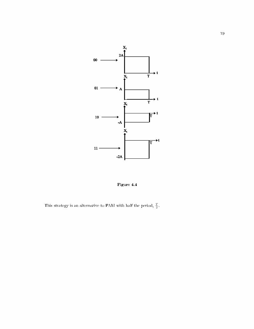
Example 4.2: ExampleData symbols are "1" or "0" and the data rate is 2

T Hertz.

19

Figure 4.4

This strategy is an alternative to PAM with half the period, T2 .


Figure 4.5

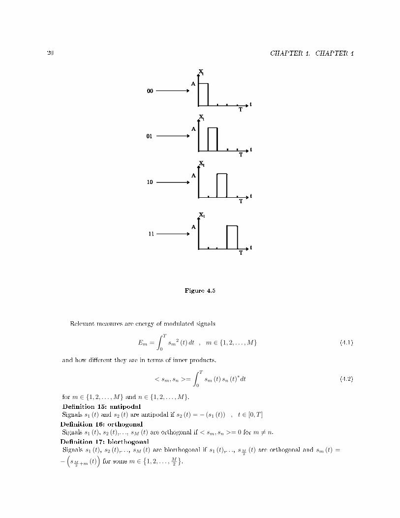
Relevant measures are energy of modulated signals

Em =∫ T

0

sm2 (t) dt , m ∈ 1, 2, . . . ,M (4.1)

and how dierent they are in terms of inner products.

< sm, sn >=∫ T

0

sm (t) sn (t)∗dt (4.2)

for m ∈ 1, 2, . . . ,M and n ∈ 1, 2, . . . ,M.Denition 15: antipodalSignals s1 (t) and s2 (t) are antipodal if s2 (t) = − (s1 (t)) , t ∈ [0, T ]Denition 16: orthogonalSignals s1 (t), s2 (t),. . ., sM (t) are orthogonal if < sm, sn >= 0 for m 6= n.

Denition 17: biorthogonalSignals s1 (t), s2 (t),. . ., sM (t) are biorthogonal if s1 (t),. . ., sM

2(t) are orthogonal and sm (t) =

−(sM

2 +m (t))for some m ∈

1, 2, . . . , M

2

.

21

It is quite intuitive to expect that the smaller (the more negative) the inner products, < sm, sn > for allm 6= n, the better the signal set.

Denition 18: Simplex signalsLet s1 (t) , s2 (t) , . . . , sM (t) be a set of orthogonal signals with equal energy. The signals s1 (t),. . .,˜sM (t) are simplex signals if

sm (t) = sm (t)− 1M

M∑k=1

(sk (t)) (4.3)

If the energy of orthogonal signals is denoted by

Es =∫ T

0

sm2 (t) dt , m ∈ 1, 2, ...,M (4.4)

then the energy of simplex signals

Es =(

1− 1M

)Es (4.5)

and

< sm, sn >=−1

M − 1Es , m 6= n (4.6)

It is conjectured that among all possible M -ary signals with equal energy, the simplex signal set resultsin the smallest probability of error when used to transmit information through an additive white Gaussiannoise channel.

The geometric representation of signals (Section 4.3) can provide a compact description of signals andcan simplify performance analysis of communication systems using the signals.

Once signals have been modulated, the receiver must detect and demodulate (Section 4.4) the signalsdespite interference and noise and decide which of the set of possible transmitted signals was sent.

4.3 Geometric Representation of Modulation Signals3

Geometric representation of signals can provide a compact characterization of signals and can simplifyanalysis of their performance as modulation signals.

Orthonormal bases are essential in geometry. Let s1 (t) , s2 (t) , . . . , sM (t) be a set of signals.Dene ψ1 (t) = s1(t)√

E1where E1 =

∫ T

0s1

2 (t) dt.

Dene s21 =< s2, ψ1 >=∫ T

0s2 (t)ψ1 (t)∗dt and ψ2 (t) = 1√

E2

(s2 (t)− s21ψ1) where E2 =∫ T

0(s2 (t)− s21ψ1 (t))2dtIn general

ψk (t) =1√Ek

sk (t)−k−1∑j=1

(skjψj (t))

(4.7)

where Ek =∫ T

0

(sk (t)−

∑k−1j=1 (skjψj (t))

)2

dt.

The process continues until all of the M signals are exhausted. The results are N orthogonal signalswith unit energy, ψ1 (t) , ψ2 (t) , . . . , ψN (t) where N ≤ M . If the signals s1 (t) , . . . , sM (t) are linearlyindependent, then N = M .



The M signals can be represented as

sm (t) =N∑

n=1

(smnψn (t)) (4.8)

with m ∈ 1, 2, . . . ,M where smn =< sm, ψn > and Em =∑N

n=1

(smn

2). The signals can be represented

by sm =

sm1

sm2

...

smN

Example 4.3

Figure 4.6

ψ1 (t) =s1 (t)√A2T

(4.9)

s11 = A√T (4.10)

s21 = −(A√T)

(4.11)

ψ2 (t) = (s2 (t)− s21ψ1 (t)) 1√E2

=(−A+ A

√T√

T

)1√E2

= 0

(4.12)

23

Figure 4.7

Dimension of the signal set is 1 with E1 = s112 and E2 = s21

2.

Example 4.4

Figure 4.8

ψm (t) = sm(t)√Es

where Es =∫ T

0sm

2 (t) dt = A2T4

s1 =

√Es

0

0

0

, s2 =

0

√Es

0

0

, s3 =

0

0√Es

0

, and s4 =

0

0

0√Es

dmn = |sm − sn| =

√√√√ N∑j=1

((smj − snj)

2)

=√

2Es , (4.13)

is the Euclidean distance between signals.

Example 4.5Set of 4 equal energy biorthogonal signals. s1 (t) = s (t), s2 (t) = s⊥ (t), s3 (t) = − (s (t)), s4 (t) =−(s⊥ (t)

).

The orthonormal basis ψ1 (t) = s(t)√Es, ψ2 (t) = s⊥(t)√

Eswhere Es =

∫ T

0sm

2 (t) dt

s1 =

√Es

0

, s2 =

0√Es

, s3 =

−(√Es

)0

, s4 =

0

−(√Es

). The four signals

can be geometrically represented using the 4-vector of projection coecients s1, s2, s3, and s4 as aset of constellation points.


Signal constellation

Figure 4.9

d21 = |s2 − s1|=

√2Es

(4.14)

d12 = d23

= d34

= d14

(4.15)

d13 = |s1 − s3|= 2

√Es

(4.16)

d13 = d24 (4.17)

Minimum distance dmin =√

2Es

4.4 Demodulation and Detection4

Consider the problem where signal set, s1, s2, . . . , sM, for t ∈ [0, T ] is used to transmit log2M bits. Themodulated signal Xt could be s1, s2, . . . , sM during the interval 0 ≤ t ≤ T .


25

Figure 4.10: rt = Xt + Nt = sm (t) + Nt for 0 ≤ t ≤ T for some m ∈ 1, 2, . . . , M.

Recall sm (t) =∑N

n=1 (smnψn (t)) for m ∈ 1, 2, . . . ,M the signals are decomposed into a set of or-thonormal signals, perfectly.

Noise process can also be decomposed

Nt =N∑

n=1

(ηnψn (t)) + Nt (4.18)

where ηn =∫ T

0Ntψn (t) dt is the projection onto the nth basis signal, Nt is the left over noise.

The problem of demodulation and detection is to observe rt for 0 ≤ t ≤ T and decide which one of theM signals were transmitted. Demodulation is covered here (Section 4.5). A discussion about detection canbe found here (Section 4.6).

4.5 Demodulation5

4.5.1 Demodulation

Convert the continuous time received signal into a vector without loss of information (or performance).

rt = sm (t) +Nt (4.19)

rt =N∑

n=1

(smnψn (t)) +N∑

n=1

(ηnψn (t)) + Nt (4.20)

rt =N∑

n=1

((smn + ηn)ψn (t)) + Nt (4.21)

rt =N∑

n=1

(rnψn (t)) + Nt (4.22)

Proposition 4.1:The noise projection coecients ηn's are zero mean, Gaussian random variables and are mutuallyindependent if Nt is a white Gaussian process.Proof:

µη (n) = E [ηn]

= E[∫ T

0Ntψn (t) dt

] (4.23)



µη (n) =∫ T

0E [Nt]ψn (t) dt

= 0(4.24)

E [ηkηn∗] = E

[∫ T

0Ntψk (t) dt

∫ T

0Nt′

∗ψk (t′)∗dt′]

=∫ T

0

∫ T

0NtNt′

∗ψk (t)ψn (t′) dtdt′(4.25)

E [ηkηn∗] =

∫ T

0

∫ T

0

RN (t− t′)ψk (t)ψn∗dtdt′ (4.26)

E [ηkηn∗] =

N0

2

∫ T

0

∫ T

0

δ (t− t′)ψk (t)ψn (t′)∗dtdt′ (4.27)

E [ηkηn∗] = N0

2

∫ T

0ψk (t)ψn (t)∗dt

= N02 δkn

=

N02 if k = n

0 if k 6= n

(4.28)

ηk 's are uncorrelated and since they are Gaussian they are also independent. Therefore, ηk ≈Gaussian

(0, N0

2

)and Rη (k, n) = N0

2 δkn

Proposition 4.2:The rn's, the projection of the received signal rt onto the orthonormal bases ψn (t)'s, are indepen-dent from the residual noise process Nt.

The residual noise Nt is irrelevant to the decision process on rt.Proof: Recall rn = smn + ηn, given sm (t) was transmitted. Therefore,

µr (n) = E [smn + ηn]

= smn

(4.29)

V ar (rn) = V ar (ηn)

= N02

(4.30)

The correlation between rn and Nt

E[Ntrn

∗]

= E

[(Nt −

N∑k=1

(ηkψk (t))

)smn + ηn

∗

](4.31)

E[Ntrn

∗]

= E

[Nt −

N∑k=1

(ηkψk (t))

]smn + E [ηkηn

∗]−N∑

k=1

(E [ηkηn∗]ψk (t)) (4.32)

E[Ntrn

∗]

= E

[Nt

∫ T

0

Nt′∗ψn (t′)∗dt′

]−

N∑k=1

(N0

2δknψk (t)

)(4.33)

E[Ntrn

∗]

=∫ T

0

N0

2δ (t− t′)ψn (t′) dt′ − N0

2ψn (t) (4.34)

27

E[Ntrn

∗]

= N02 ψn (t)− N0

2 ψn (t)

= 0(4.35)

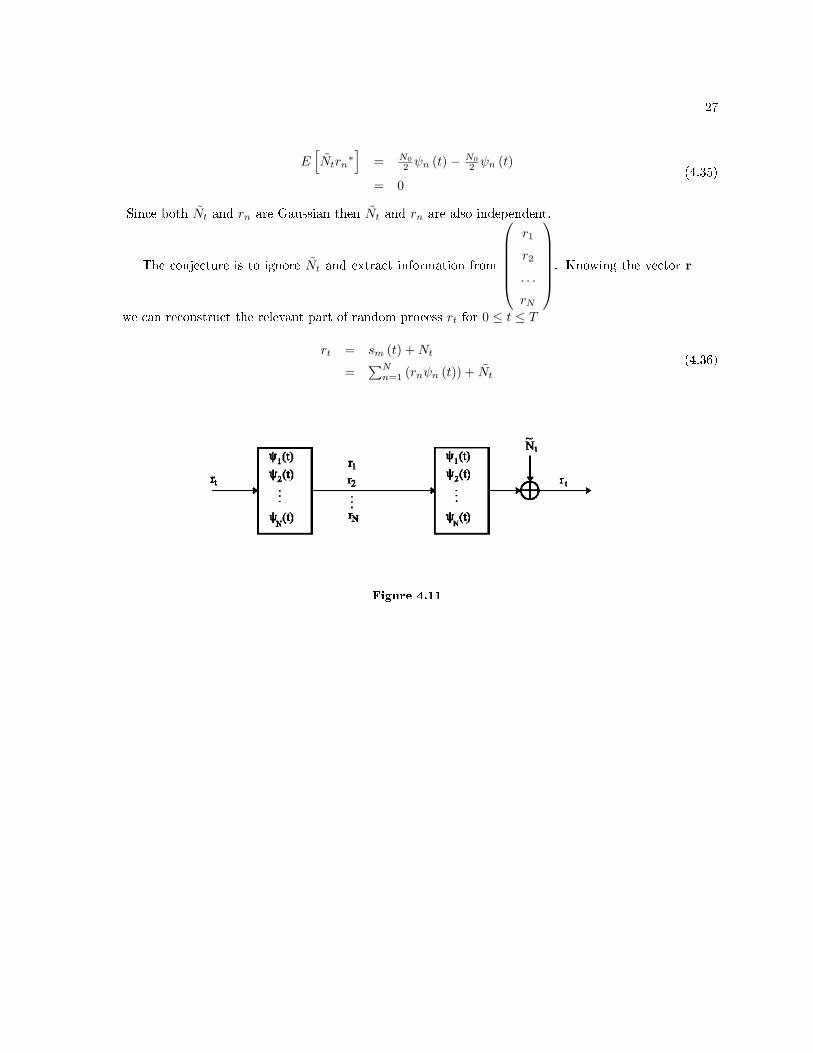
Since both Nt and rn are Gaussian then Nt and rn are also independent.

The conjecture is to ignore Nt and extract information from

r1

r2

. . .

rN

. Knowing the vector r

we can reconstruct the relevant part of random process rt for 0 ≤ t ≤ T

rt = sm (t) +Nt

=∑N

n=1 (rnψn (t)) + Nt

(4.36)

Figure 4.11


Figure 4.12

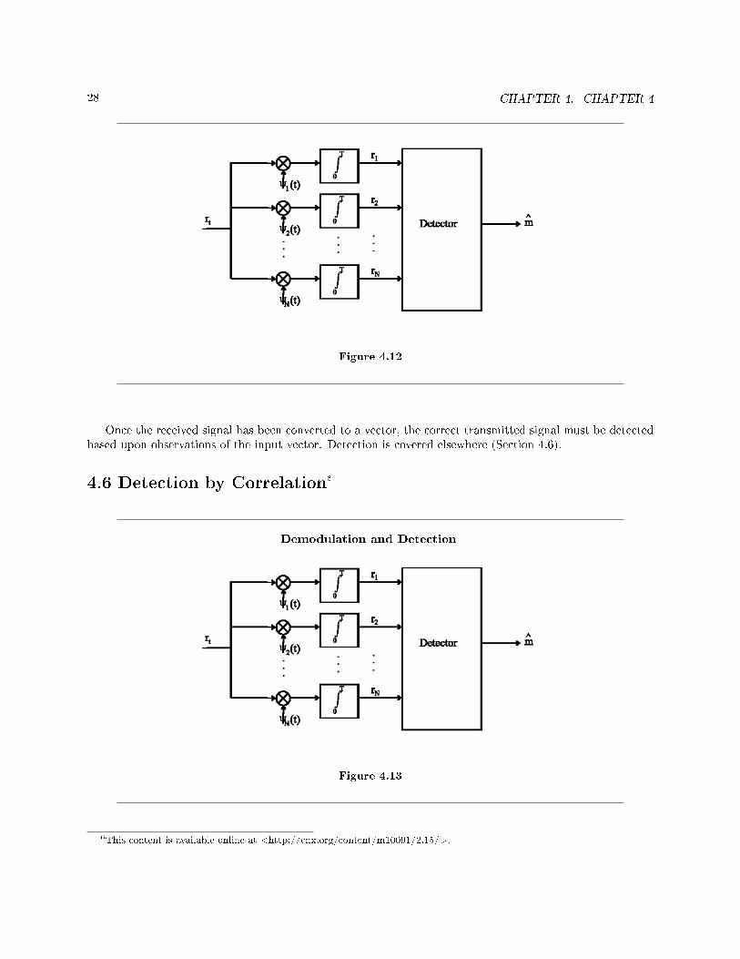
Once the received signal has been converted to a vector, the correct transmitted signal must be detectedbased upon observations of the input vector. Detection is covered elsewhere (Section 4.6).

4.6 Detection by Correlation6

Demodulation and Detection

Figure 4.13


29

4.6.1 Detection

Decide which sm (t) from the set of s1 (t) , . . . , sm (t) signals was transmitted based on observing r =r1

r2

...

rN

, the vector composed of demodulated (Section 4.5) received signal, that is, the vector of projection

of the received signal onto the N bases.

m = arg max1≤m≤M

Pr [sm (t) was transmitted | r was observed] (4.37)

Note that

Pr [sm | r] , Pr [sm (t)was transmitted | r was observed] =fr|sm

Pr [sm]fr

(4.38)

If Pr [sm was transmitted] = 1M , that is information symbols are equally likely to be transmitted, then

arg max1≤m≤M

Pr [sm | r] = arg max1≤m≤M

fr|sm(4.39)

Since r (t) = sm (t)+Nt for 0 ≤ t ≤ T and for some m = 1, 2, . . . ,M then r = sm +η where η =

η1

η2...

ηN

and ηn's are Gaussian and independent.

fr|sm=

1(2πN0

2

)N2e

−(PNn=1((rn−smn)2))

2N02 , rn ∈ R (4.40)

m = arg max1≤m≤M

fr|sm

= arg max1≤m≤M

lnfr|sm

= arg max1≤m≤M

−(

N2 ln (πN0)

)− 1

N0

∑Nn=1

((rn − smn)2

)= arg min

1≤m≤M

∑Nn=1

((rn − smn)2

)(4.41)

where D (r, sm) is the l2 distance between vectors r and sm dened as D (r, sm) ,∑N

n=1

((rn − smn)2

)m = arg min

1≤m≤MD (r, sm)

= arg min1≤m≤M

(‖ r ‖)2 −(2 < r, sm > +(‖ sm ‖)2

) (4.42)

where ‖ r ‖ is the l2 norm of vector r dened as ‖ r ‖,√∑N

n=1

((rn)2

)m = arg max

1≤m≤M2 < r, sm > −(‖ sm ‖)2 (4.43)

This type of receiver system is known as a correlation (or correlator-type) receiver. Examples of the useof such a system are found here (Section 4.7). Another type of receiver involves linear, time-invariant ltersand is known as a matched lter (Section 4.8) receiver. An analysis of the performance of a correlator-typereceiver using antipodal and orthogonal binary signals can be found in Performance Analysis (Section 4.11).


4.7 Examples of Correlation Detection7

The implementation and theory of correlator-type receivers can be found in Detection (Section 4.6).

Example 4.6

Figure 4.14

m = 2 since D (r, s1) > D (r, s2) or (‖ s1 ‖)2 = (‖ s2 ‖)2 and < r, s2 >>< r, s1 >.

Figure 4.15

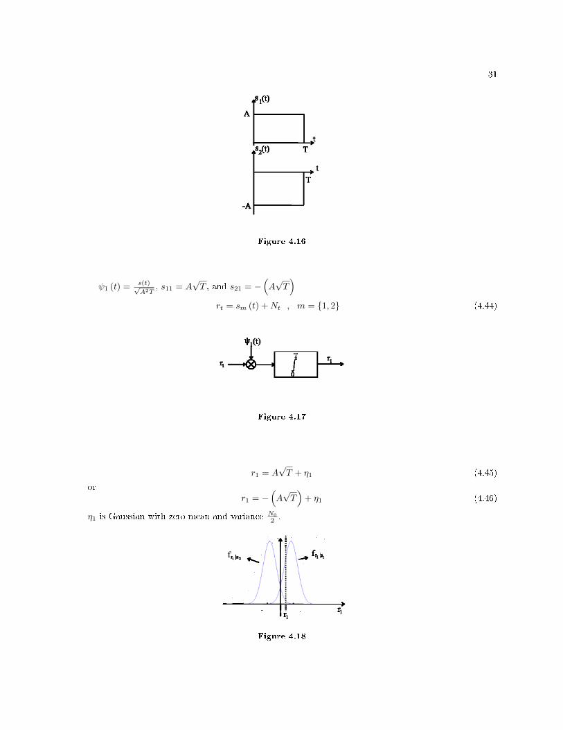
Example 4.7Data symbols "0" or "1" with equal probability. Modulator s1 (t) = s (t) for 0 ≤ t ≤ T ands2 (t) = − (s (t)) for 0 ≤ t ≤ T .


31

Figure 4.16

ψ1 (t) = s(t)√A2T

, s11 = A√T , and s21 = −

(A√T)

rt = sm (t) +Nt , m = 1, 2 (4.44)

Figure 4.17

r1 = A√T + η1 (4.45)

orr1 = −

(A√T)

+ η1 (4.46)

η1 is Gaussian with zero mean and variance N02 .

Figure 4.18


m = argmaxA√Tr1,−

(A√Tr1

), since A

√T > 0 and Pr [s1] = Pr [s1] then the MAP

decision rule decides.s1 (t) was transmitted if r1 ≥ 0s2 (t) was transmitted if r1 < 0An alternate demodulator:

rt = sm (t) +Nt ⇒ r = sm + η (4.47)

4.8 Matched Filters8

Signal to Noise Ratio (SNR) at the output of the demodulator is a measure of the quality of the demod-ulator.

SNR =signal energy

noise energy(4.48)

In the correlator described earlier, Es = (|sm|)2 and σηn2 = N0

2 . Is it possible to design a demodulatorbased on linear time-invariant lters with maximum signal-to-noise ratio?

Figure 4.19

If sm (t) is the transmitted signal, then the output of the kth lter is given as

yk (t) =∫∞−∞ rτhk (t− τ) dτ

=∫∞−∞ (sm (τ) +Nτ )hk (t− τ) dτ

=∫∞−∞ sm (τ)hk (t− τ) dτ +

∫∞−∞Nτhk (t− τ) dτ

(4.49)


33

Sampling the output at time T yields

yk (T ) =∫ ∞

−∞sm (τ)hk (T − τ) dτ +

∫ ∞

−∞Nτhk (T − τ) dτ (4.50)

The noise contribution:

νk =∫ ∞

−∞Nτhk (T − τ) dτ (4.51)

The expected value of the noise component is

E [νk] = E[∫∞−∞Nτhk (T − τ) dτ

]= 0

(4.52)

The variance of the noise component is the second moment since the mean is zero and is given as

σ(νk)2 = E[νk

2]

= E[∫∞−∞Nτhk (T − τ) dτ

∫∞−∞Nτ '

∗hk

(T − τ '

)∗dτ '] (4.53)

E[νk

2]

=∫∞−∞

∫∞−∞

N02 δ(τ − τ '

)hk (T − τ)hk

(T − τ '

)∗dτdτ '

= N02

∫∞−∞ (|hk (T − τ) |)2dτ

(4.54)

Signal Energy can be written as (∫ ∞

−∞sm (τ)hk (T − τ) dτ

)2

(4.55)

and the signal-to-noise ratio (SNR) as

SNR =

(∫∞−∞ sm (τ)hk (T − τ) dτ

)2

N02

∫∞−∞ (|hk (T − τ) |)2dτ

(4.56)

The signal-to-noise ratio, can be maximized considering the well-known Cauchy-Schwarz Inequality(∫ ∞

−∞g1 (x) g2 (x)∗dx

)2

≤∫ ∞

−∞(|g1 (x) |)2dx

∫ ∞

−∞(|g2 (x) |)2dx (4.57)

with equality when g1 (x) = αg2 (x). Applying the inequality directly yields an upper bound on SNR(∫∞−∞ sm (τ)hk (T − τ) dτ

)2

N02

∫∞−∞ (|hk (T − τ) |)2dτ

≤ 2N0

∫ ∞

−∞(|sm (τ) |)2dτ (4.58)

with equality hoptk (T − τ) = αsm (τ)∗ , . Therefore, the lter to examine signal m should be

Matched Filterτhopt

m (τ) = sm (T − τ)∗ , (4.59)

The constant factor is not relevant when one considers the signal to noise ratio. The maximum SNR isunchanged when both the numerator and denominator are scaled.

2N0

∫ ∞

−∞(|sm (τ) |)2dτ =

2Es

N0(4.60)

Examples involving matched lter receivers can be found here (Section 4.9). An analysis in the frequencydomain is contained in Matched Filters in the Frequency Domain (Section 4.10).

Another type of receiver system is the correlation (Section 4.6) receiver. A performance analysis of bothmatched lters and correlator-type receivers can be found in Performance Analysis (Section 4.11).


4.9 Examples with Matched Filters9

The theory and rationale behind matched lter receivers can be found in Matched Filters (Section 4.8).

Example 4.8

Figure 4.20

s1 (t) = t for 0 ≤ t ≤ Ts2 (t) = −t for 0 ≤ t ≤ Th1 (t) = T − t for 0 ≤ t ≤ Th2 (t) = −T + t for 0 ≤ t ≤ T

Figure 4.21

s1 (t) =∫ ∞

−∞s1 (τ)h1 (t− τ) dτ , 0 ≤ t ≤ 2T (4.61)

s1 (t) =∫ t

0τ (T − t+ τ) dτ

= 12 (T − t) τ2|t0 + 1

3τ3|t0

= t2

2

(T − t

3

) (4.62)


35

s1 (T ) =T 3

3(4.63)

Compared to the correlator-type demodulation

ψ1 (t) =s1 (t)√Es

(4.64)

s11 =∫ T

0

s1 (τ)ψ1 (τ) dτ (4.65)

∫ t

0s1 (τ)ψ1 (τ) dτ = 1√

Es

∫ t

0ττdτ

= 1√Es

13 t

3(4.66)

Figure 4.22

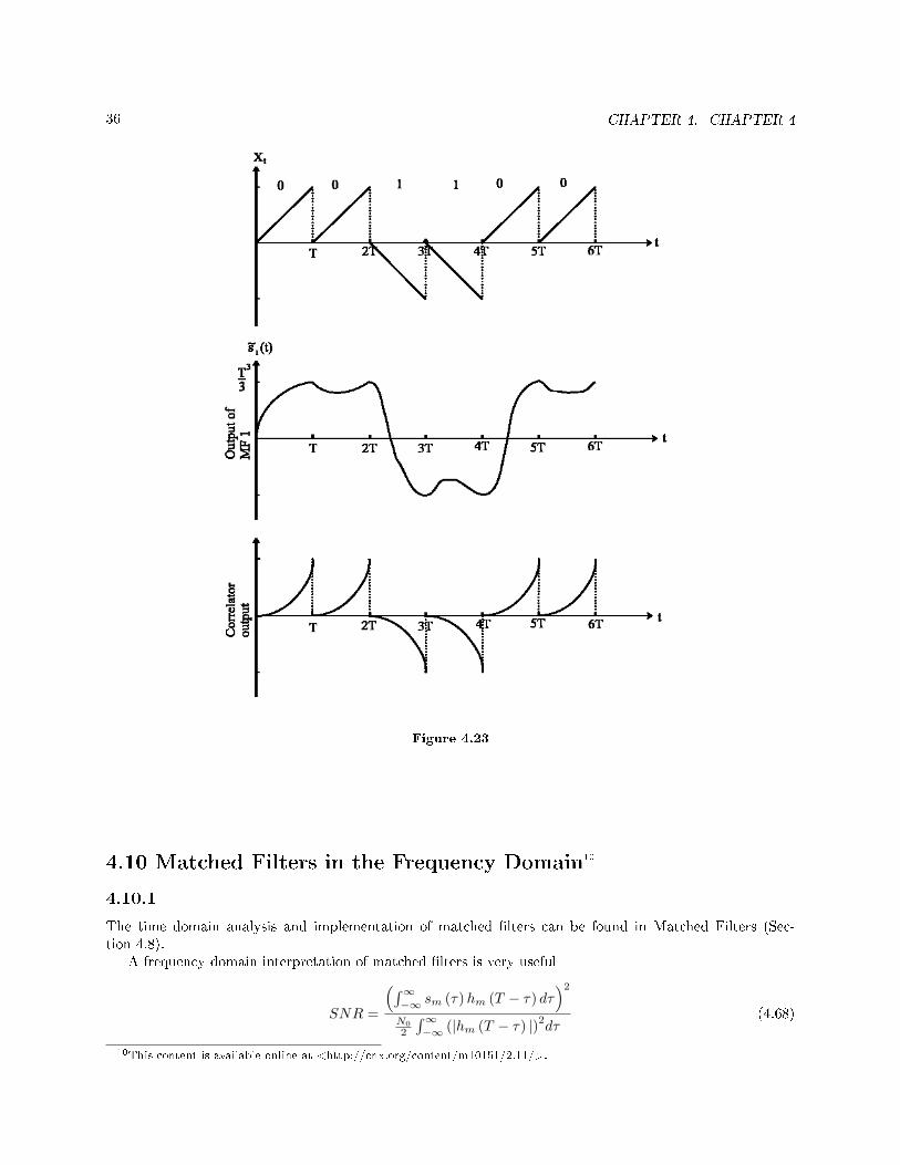
Example 4.9Assume binary data is transmitted at the rate of 1

T Hertz.0 ⇒ b = 1 ⇒ s1 (t) = s (t) for 0 ≤ t ≤ T1 ⇒ b = −1 ⇒ s2 (t) = − (s (t)) for 0 ≤ t ≤ T

Xt =P∑

i=−P

(bis (t− iT )) (4.67)


Figure 4.23

4.10 Matched Filters in the Frequency Domain10

4.10.1

The time domain analysis and implementation of matched lters can be found in Matched Filters (Sec-tion 4.8).

A frequency domain interpretation of matched lters is very useful

SNR =

(∫∞−∞ sm (τ)hm (T − τ) dτ

)2

N02

∫∞−∞ (|hm (T − τ) |)2dτ

(4.68)


37

For the m-th lter, hm can be expressed as

sm (T ) =∫∞−∞ sm (τ)hm (T − τ) dτ

= F−1 (Hm (f)Sm (f))

=∫∞−∞Hm (f)Sm (f) ej2πfT df

(4.69)

where the second equality is because∼sm is the lter output with input Sm and lter Hm and we can now

dene Hm (f) = Hm (f)∗e−(j2πfT ) , then

sm (T ) =< Sm (f) , Hm (f) > (4.70)

The denominator ∫ ∞

−∞(|hm (T − τ) |)2dτ =

∫ ∞

−∞(|hm (τ) |)2dτ (4.71)

hm ∗ hm (0) =∫∞−∞ (|Hm (f) |)2df

= < Hm (f) ,Hm (f) >(4.72)

hm ∗ hm (0) =∫∞−∞Hm (f) ej2πfTHm (f)∗e−(j2πfT )df

= < Hm (f) , Hm (f) >(4.73)

Therefore,

SNR =

(< Sm (f) , Hm (f) >

)2

N02 < Hm (f) , Hm (f) >

≤ 2N0

< Sm (f) , Sm (f) > (4.74)

with equality whenHm (f) = αSm (f) (4.75)

or

Matched Filter in the frequency domain

Hm (f) = Sm (f)∗e−(j2πfT ) (4.76)

Matched Filter

Figure 4.24

sm (t) = F−1(sm (f) sm (f)∗

)=

∫∞−∞ (|sm (f) |)2ej2πftdf

=∫∞−∞ (|sm (f) |)2cos (2πft) df

(4.77)


where F−1 is the inverse Fourier Transform operator.

4.11 Performance Analysis11

In this section we will evaluate the probability of error of both correlator type receivers and matched lterreceivers. We will only present the analysis for transmission of binary symbols. In the process we willdemonstrate that both of these receivers have identical bit-error probabilities.

4.11.1 Antipodal Signals

rt = sm (t) +Nt for 0 ≤ t ≤ T with m = 1 and m = 2 and s1 (t) = − (s2 (t))An analysis of the performance of correlation receivers with antipodal binary signals can be found here

(Section 4.12). A similar analysis for matched lter receivers can be found here (Section 4.14).

4.11.2 Orthogonal Signals

rt = sm (t) +Nt for 0 ≤ t ≤ T with m = 1 and m = 2 and < s1, s2 >= 0An analysis of the performance of correlation receivers with orthogonal binary signals can be found here

(Section 4.13). A similar analysis for matched lter receivers can be found here (Section 4.15).It can be shown in general that correlation and matched lter receivers perform with the same symbol

error probability if the detection criteria is the same for both receivers.

4.12 Performance Analysis of Antipodal Binary signals with

Correlation12

Figure 4.25

The bit-error probability for a correlation receiver with an antipodal signal set (Figure 4.25) can be foundas follows:

Pe = Pr [m 6= m]

= Pr[b 6= b

]= π0Pr [r1 < γ|m=1] + π1Pr [r1 ≥ γ|m=2]

= π0

∫ γ

−∞ f r1,s1(t) (r ) dr + π1

∫∞γf r1,s2(t) (r ) dr

(4.78)


39

if π0 = π1 = 1/2, then the optimum threshold is γ = 0.

f (r1|s1(t)) (r ) = [U+EF3B]

(√Es,

N0

2

)(4.79)

f (r1|s2(t)) (r ) = [U+EF3B]

(−(√

Es

),N0

2

)(4.80)

If the two symbols are equally likely to be transmitted then π0 = π1 = 1/2 and if the threshold is set tozero, then

Pe = 1/2∫ 0

−∞

1√2πN0

2

e−„

(|r−√

Es|)2

N0

«dr + 1/2

∫ ∞

0

1√2πN0

2

e−„

(|r+√

Es|)2

N0

«dr (4.81)

Pe = 1/2∫ −

“q2EsN0

”−∞

1√2πe−((|r′|)2)

2 dr′ + 1/2∫ ∞q

2EsN0

1√2πe

− „

|r′′|«2!

2 dr′′

(4.82)

with r′ = r−√

EsqN02

and r′′

= r+√

EsqN02

Pe = 12Q(√

2Es

N0

)+ 1

2Q(√

2Es

N0

)= Q

(√2Es

N0

) (4.83)

where Q (b) =∫∞

b1√2πe−(x2)

2 dx.

Note that

Figure 4.26

Pe = Q

(d12√2N0

)(4.84)

where d12 = 2√Es = (‖ s1 − s2 ‖)2 is the Euclidean distance between the two constellation points (Fig-

ure 4.26).This is exactly the same bit-error probability as for the matched lter case.A similar bit-error analysis for matched lters can be found here (Section 4.14). For the bit-error analysis

for correlation receivers with an orthogonal signal set, refer here (Section 4.13).

4.13 Performance Analysis of Binary Orthogonal Signals with

Correlation13

Orthogonal signals with equally likely bits, rt = sm (t)+Nt for 0 ≤ t ≤ T , m = 1, m = 2, and < s1, s2 >= 0.



4.13.1 Correlation (correlator-type) receiver

rt ⇒ r = (r1, r2)T = sm + η (see Figure 4.27)

Figure 4.27

Decide s1 (t) was transmitted if r1 ≥ r2.

Pe = Pr [m 6= m]

= Pr[b 6= b

] (4.85)

Pe = 1/2Pr [r ∈ R2 | s1 (t) transmitted] + 1/2Pr [r ∈ R1 | s2 (t) transmitted] =1/2∫R2

∫f r,s1(t) (r) dr1dr2 + 1/2

∫R1

∫f r,s2(t) (r) dr1dr2 =

1/2∫R2

∫1q

2πN02

e−((|r1−

√Es|)2)

N01√πN0

e−((|r2|)

2)N0 dr1dr2+1/2

∫R1

∫1q

2πN02

e−((|r1|)

2)N0

1√πN0

e−((|r2−

√Es|)2)

N0 dr1dr2

(4.86)

Alternatively, if s1 (t) is transmitted we decide on the wrong signal if r2 > r1 or η2 > η1 +√Es or when

η2 − η1 >√Es.

Pe = 1/2∫∞√

Es

1√2πN0

e−(η′2)

2N0 dη′ + 1/2Pr [r1 ≥ r2 | s2 (t) transmitted]

= Q(√

Es

N0

) (4.87)

Note that the distance between s1 and s2 is d12 =√

2Es. The average bit error probability Pe = Q(

d12√2N0

)as we had for the antipodal case (Section 4.12). Note also that the bit-error probability is the same as forthe matched lter (Section 4.15) receiver.

41

4.14 Performance Analysis of Binary Antipodal Signals with

Matched Filters14

4.14.1 Matched Filter receiver

Recall rt = sm (t) +Nt where m = 1 or m = 2 and s1 (t) = − (s2 (t)) (see Figure 4.28).

Figure 4.28

Y1 (T ) = Es + ν1 (4.88)

Y2 (T ) = −Es + ν2 (4.89)

since s1 (t) = − (s2 (t)) then ν1 is [U+EF3B](0, N0

2 Es

). Furthermore ν2 = −ν1. Given ν1 then ν2 is

deterministic and equals −ν1. Then Y2 (T ) = − (Y1 (T )) if s1 (t) is transmitted.If s2 (T ) is transmitted

Y1 (T ) = −Es + ν1 (4.90)

Y2 (T ) = Es + ν2 (4.91)

ν1 is [U+EF3B](0, N0

2 Es

)and ν2 = −ν1.

The receiver can be simplied to (see Figure 4.29)

Figure 4.29

If s1 (t) is transmitted Y1 (T ) = Es + ν1.



If s2 (t) is transmitted Y1 (T ) = −Es + ν1.

Pe = 1/2Pr [Y1 (T ) < 0 | s1 (t)] + 1/2Pr [Y1 (T ) ≥ 0 | s2 (t)]

= 1/2∫ 0

−∞1q

2πN02 Es

e−((|y−Es|)2)

N0Es dy + 1/2∫∞0

1q2π

N02 Es

e−((|y+Es|)2)

N0Es dy

= Q

(EsqN02 Es

)= Q

(√2Es

N0

)(4.92)

This is the exact bit-error rate of a correlation receiver (Section 4.12). For a bit-error analysis for orthogonalsignals using a matched lter receiver, refer here (Section 4.15).

4.15 Performance Analysis of Orthogonal Binary Signals with

Matched Filters15

rt ⇒ Y =

Y1 (T )

Y2 (T )

(4.93)

If s1 (t) is transmitted

Y1 (T ) =∫∞−∞ s1 (τ)hopt

1 (T − τ) dτ + ν1 (T )

=∫∞−∞ s1 (τ) s∗1 (τ) dτ + ν1 (T )

= Es + ν1 (T )

(4.94)

Y2 (T ) =∫∞−∞ s1 (τ) s∗2 (τ) dτ + ν2 (T )

= ν2 (T )(4.95)

If s2 (t) is transmitted, Y1 (T ) = ν1 (T ) and Y2 (T ) = Es + ν2 (T ).


43

Figure 4.30

H0

Y =

Es

0

+

ν1

ν2

(4.96)

H1

Y =

0

Es

+

ν1

ν2

(4.97)

where ν1 and ν2 are independent are Gaussian with zero mean and variance N02 Es. The analysis is identical

to the correlator example (Section 4.13).

Pe = Q

(√Es

N0

)(4.98)

Note that the maximum likelihood detector decides based on comparing Y1 and Y2. If Y1 ≥ Y2 thens1 was sent; otherwise s2 was transmitted. For a similar analysis for binary antipodal signals, refer here(Section 4.14). See Figure 4.31 or Figure 4.32.


Figure 4.31

Figure 4.32

Chapter 5

Chapter 5

5.1 Digital Transmission over Baseband Channels1

Until this point, we have considered data transmissions over simple additive Gaussian channels that are nottime or band limited. In this module we will consider channels that do have bandwidth constraints, and arelimited to frequency range around zero (DC). The channel is best modied as g (t) is the impulse responseof the baseband channel.

Consider modulated signals xt = sm (t) for 0 ≤ t ≤ T for some m ∈ 1, 2, . . . ,M . The channel outputis then

rt =∫∞−∞ xτg (t− τ) dτ +Nt

=∫∞−∞ Sm (τ) g (t− τ) dτ +Nt

(5.1)

The signal contribution in the frequency domain is

Sm (f) = Sm (f)G (f) , (5.2)

The optimum matched lter should match to the ltered signal:

Hoptm (f) = Sm (f)∗G (f)∗e(−j)2πft , (5.3)

This lter is indeed optimum (i.e., it maximizes signal-to-noise ratio); however, it requires knowledge ofthe channel impulse response. The signal energy is changed to

Es =∫ ∞

−∞

(|Sm (f) |

)2

df (5.4)

The band limited nature of the channel and the stream of time limited modulated signal create aliasingwhich is referred to as intersymbol interference. We will investigate ISI for a general PAM signaling.

5.2 Pulse Amplitude Modulation Through Bandlimited Channel2

Consider a PAM system b−10,. . ., b−1, b0 b1,. . .This implies

xt =∞∑

n=−∞(ans (t− nT )) , an ∈ M levels of amplitude (5.5)


45


The received signal is

rt =∫∞−∞

(∑∞n=−∞ (ans (t− (τ − nT )))

)g (τ) dτ +Nt

=∑∞

n=−∞

(an

∫∞−∞ s (t− (τ − nT )) g (τ) dτ

)+Nt

=∑∞

n=−∞ (ans (t− nT ) +Nt)

(5.6)

Since the signals span a one-dimensional space, one lter matched to s (t) = s∗g (t) is sucient.The matched lter's impulse response is

hopt (t) = s∗g (T − t) , (5.7)

The matched lter output is

y (t) =∫∞−∞

∑∞n=−∞ (ans (t− (τ − nT ))hopt (τ)) dτ + ν (t)

=∑∞

n=−∞

(an

∫∞−∞ s (t− (τ − nT ))hopt (τ) dτ

)+ ν (t)

=∑∞

n=−∞ (anu (t− nT )) + ν (t)

(5.8)

The decision on the kth symbol is obtained by sampling the MF output at kT :

y (kT ) =∞∑

n=−∞(anu (kT − nT )) + ν (kT ) (5.9)

The kth symbol is of interest:

y (kT ) = aku (0) +∞∑

n=−∞(anu (kT − nT )) + ν (kT ) (5.10)

where n 6= k.Since the channel is bandlimited, it provides memory for the transmission system. The eect of old

symbols (possibly even future signals) lingers and aects the performance of the receiver. The eect ofISI can be eliminated or controlled by proper design of modulation signals or precoding lters at thetransmitter, or by equalizers or sequence detectors at the receiver.

5.3 Precoding and Bandlimited Signals3

5.3.1 Precoding

The data symbols are manipulated such that

yk (kT ) = aku (0) + ISI + ν (kT ) (5.11)


47

5.3.2 Design of Bandlimited Modulation Signals

Recall that modulation signals are

Xt =∞∑

n=−∞(ans (t− nT )) (5.12)

We can design s (t) such that

u (nT ) =

large if n = 0

zero or small if n 6= 0(5.13)

where y (kT ) = aku (0) +∑∞

n=−∞ (anu (kT − nT )) + ν (kT ) (ISI is the sum term, and once again, n 6= k .)Also, y (nT ) = s∗g∗hopt (nT ) The signal s (t) can be designed to have reduced ISI.

5.3.3 Design Equalizers at the Receiver

Linear equalizers or decision feedback equalizers reduce ISI in the statistic yt

5.3.4 Maximum Likelihood Sequence Detection

y (kT ) =∞∑

n=−∞(an (kT − nT )) + ν (k (T )) (5.14)

By observing y (T ) , y (2T ) , . . . the date symbols are observed frequently. Therefore, ISI can be viewed asdiversity to increase performance.

Chapter 6

Chapter 6

6.1 Carrier Phase Modulation1

6.1.1 Phase Shift Keying (PSK)

Information is impressed on the phase of the carrier. As data changes from symbol period to symbol period,the phase shifts.

sm (t) = APT (t) cos(

2πfct+2π (m− 1)

M

), m ∈ 1, 2, . . . ,M (6.1)

Example 6.1Binary s1 (t) or s2 (t)

6.1.2 Representing the Signals

An orthonormal basis to represent the signals is

ψ1 (t) =1√Es

APT (t) cos (2πfct) (6.2)

ψ2 (t) =−1√Es

APT (t) sin (2πfct) (6.3)

The signal

Sm (t) = APT (t) cos(

2πfct+2π (m− 1)

M

)(6.4)

Sm (t) = Acos

(2π (m− 1)

M

)PT (t) cos (2πfct)−Asin

(2π (m− 1)

M

)PT (t) sin (2πfct) (6.5)

The signal energy

Es =∫∞−∞A2PT

2 (t) cos2(2πfct+ 2π(m−1)

M

)dt

=∫ T

0A2(

12 + 1

2cos(4πfct+ 4π(m−1)

M

))dt

(6.6)


49


Es =A2T

2+

12A2

∫ T

0

cos

(4πfct+

4π (m− 1)M

)dt ≈ A2T

2(6.7)

(Note that in the above equation, the integral in the last step before the aproximation is very small.)Therefore,

ψ1 (t) =

√2TPT (t) cos (2πfct) (6.8)

ψ2 (t) =

(−

(√2T

))PT (t) sin (2πfct) (6.9)

In general,

sm (t) = APT (t) cos(

2πfct+2π (m− 1)

M

), m ∈ 1, 2, . . . ,M (6.10)

and ψ1 (t)

ψ1 (t) =

√2TPT (t) cos (2πfct) (6.11)

ψ2 (t) =

√2TPT (t) sin (2πfct) (6.12)

sm =

√Escos

(2π(m−1)

M

)√Essin

(2π(m−1)

M

) (6.13)

6.1.3 Demodulation and Detection

rt = sm (t) +Nt, for somem ∈ 1, 2, . . . ,M (6.14)

We must note that due to phase oset of the oscillator at the transmitter, phase jitter or phase changesoccur because of propagation delay.

rt = APT (t) cos(

2πfct+2π (m− 1)

M+ φ

)+Nt (6.15)

For binary PSK, the modulation is antipodal, and the optimum receiver in AWGN has average bit-errorprobability

Pe = Q(√

2Es

N0

)= Q

(A√

TN0

) (6.16)

The receiver wherert = ±APT (t) cos (2πfct+ φ) +Nt (6.17)

The statistics

r1 =∫ T

0rtαcos

(2πfct+ φ

)dt

= ±∫ T

0αAcos (2πfct+ φ) cos

(2πfct+ φ

)dt+

∫ T

0αcos

(2πfct+ φ

)Ntdt

(6.18)

r1 = ±

(αA

2

∫ T

0

cos(4πfct+ φ+ φ

)+ cos

(φ− φ

)dt

)+ η1 (6.19)

51

r1 = ±αA2Tcos

(φ− φ

)+∫ T

0

±(αA

2cos(4πfct+ φ+ φ

))dt+ η1 ≈ ±

(αAT

2cos(φ− φ

))+ η1 (6.20)

where η1 = α∫ T

0Ntcos

(ωct+ φ

)dt is zero mean Gaussian with variance ≈ α2N0T

4 .

Therefore,

Pe = Q

(2 αAT

2 cos(φ−φ)2

qα2N0T

4

)= Q

(cos(φ− φ

)A√

TN0

) (6.21)

which is not a function of α and depends strongly on phase accuracy.

Pe = Q

(cos(φ− φ

)√2Es

N0

)(6.22)

The above result implies that the amplitude of the local oscillator in the correlator structure does not playa role in the performance of the correlation receiver. However, the accuracy of the phase does indeed play amajor role. This point can be seen in the following example:

Example 6.2

xt′ = −1iAcos (− (2πfct′) + 2πfcτ) (6.23)

xt = −1iAcos (2πfct− (2πfcτ′ − (2πfcτ + θ′))) (6.24)

Local oscillator should match to phase θ.

6.2 Dierential Phase Shift Keying2

The phase lock loop provides estimates of the phase of the incoming modulated signal. A phase ambiguityof exactly π is a common occurance in many phase lock loop (PLL) implementations.

Therefore it is possible that, θ = θ + π without the knowledge of the receiver. Even if there is no noise,if b = 1 then b = 0 and if b = 0 then b = 1.

In the presence of noise, an incorrect decision due to noise may results in a correct nal desicion (inbinary case, when there is π phase ambiguity with the probability:

Pe = 1−Q

(√2Es

N0

)(6.25)

Consider a stream of bits an ∈ 0, 1 and BPSK modulated signal∑n

(−1anAPT (t− nT ) cos (2πfct+ θ)) (6.26)

In dierential PSK, the transmitted bits are rst encoded bn = (an ⊕ bn−1) with initial symbol (e.g. b0)chosen without loss of generality to be either 0 or 1.

Transmitted DPSK signals ∑n

(−1bnAPT (t− nT ) cos (2πfct+ θ)

)(6.27)



The decoder can be constructed as

(bn−1 ⊕ bn) = (bn−1 ⊕ an ⊕ bn−1)

= (0⊕ an)

= an

(6.28)

If two consecutive bits are detected correctly, if bn = bn and bn−1 = bn−1 then

an =(bn ⊕ bn−1

)= (bn ⊕ bn−1)

= (an ⊕ bn−1 ⊕ bn−1)

= an

(6.29)

if bn = (bn ⊕ 1) and bn−1 = (bn−1 ⊕ 1). That is, two consecutive bits are detected incorrectly. Then,

an =(bn ⊕ bn−1

)= (bn ⊕ 1⊕ bn−1 ⊕ 1)

= (bn ⊕ bn−1 ⊕ 1⊕ 1)

= (bn ⊕ bn−1 ⊕ 0)

= (bn ⊕ bn−1)

= an

(6.30)

If bn = (bn ⊕ 1) and bn−1 = bn−1, that is, one of two consecutive bits is detected in error. In this case therewill be an error and the probability of that error for DPSK is

P e = Pr [an 6= an]

= Pr[bn = bn, bn−1 6= bn−1

]+ Pr

[bn 6= bn, bn−1 = bn−1

]= 2Q

(√2Es

N0

) [1−Q

(√2Es

N0

)]≈ 2Q

(√2Es

N0

) (6.31)

This approximation holds if Q is small.

6.3 Carrier Frequency Modulation3

6.3.1 Frequency Shift Keying (FSK)

The data is impressed upon the carrier frequency. Therefore, the M dierent signals are

sm (t) = APT (t) cos (2πfct+ 2π (m− 1) ∆ft+ θm) (6.32)

for m ∈ 1, 2, . . . ,MThe M dierent signals have M dierent carrier frequencies with possibly dierent phase angles since

the generators of these carrier signals may be dierent. The carriers are

f1 = fc (6.33)


53

f2 = fc + ∆f

fM = fc + (M − 1) ∆f

Thus, the M signals may be designed to be orthogonal to each other.

< sm, sn >=∫ T

0A2cos (2πfct + 2π (m− 1) ∆ft + θm) cos (2πfct + 2π (n− 1) ∆ft + θn) dt =

A2

2

∫ T

0cos (4πfct + 2π (n + m− 2) ∆ft + θm + θn) dt+A2

2

∫ T

0cos (2π (m− n) ∆ft + θm − θn) dt =

A2

2sin(4πfcT+2π(n+m−2)∆fT+θm+θn)−sin(θm+θn)

4πfc+2π(n+m−2)∆f+A2

2

(sin(2π(m−n)∆fT+θm−θn)

2π(m−n)∆f− sin(θm−θn)

2π(m−n)∆f

)(6.34)

If 2fcT + (n+m− 2) ∆fT is an integer, and if (m− n) ∆fT is also an integer, then < Sm, Sn >= 0 if∆fT is an integer, then < sm, sn >≈ 0 when fc is much larger than 1

T .In case , θm = 0

< sm, sn >≈A2T

2sinc (2 (m− n) ∆fT ) (6.35)

Therefore, the frequency spacing could be as small as ∆f = 12T since sinc (x) = 0 if x = ±1 or ±2.

If the signals are designed to be orthogonal then the average probability of error for binary FSK withoptimum receiver is

−P e = Q

(√Es

N0

)(6.36)

in AWGN.Note that sinc (x) takes its minimum value not at x = ±1 but at ±1.4 and the minimum value is −0.216.

Therefore if ∆f = 0.7T then

−P e = Q

(√1.216Es

N0

)(6.37)

which is a gain of 10log1.216 ≈ 0.85dθ over orthogonal FSK.

Chapter 7

Chapter 7

7.1 Information Theory and Coding1

In the previous chapters, we considered the problem of digital transmission over dierent channels. Infor-mation sources are not often digital, and in fact, many sources are analog. Although many channels are alsoanalog, it is still more ecient to convert analog sources into digital data and transmit over analog channelsusing digital transmission techniques. There are two reasons why digital transmission could be more ecientand more reliable than analog transmission:

1. Analog sources could be compressed to digital form eciently.2. Digital data can be transmitted over noisy channels reliably.

There are several key questions that need to be addressed:

1. How can one model information?2. How can one quantify information?3. If information can be measured, does its information quantity relate to how much it can be compressed?4. Is it possible to determine if a particular channel can handle transmission of a source with a particular

information quantity?

Figure 7.1

Example 7.1The information content of the following sentences: "Hello, hello, hello." and "There is an examtoday." are not the same. Clearly the second one carries more information. The rst one can becompressed to "Hello" without much loss of information.

In other modules, we will quantify information and nd ecient representation of information (Entropy (Sec-tion 7.2)). We will also quantify how much (Section 7.5) information can be transmitted through channels,reliably. Channel coding (Section 7.9) can be used to reduce information rate and increase reliability.


55


7.2 Entropy2

Information sources take very dierent forms. Since the information is not known to the destination, it isthen best modeled as a random process, discrete-time or continuous time.

Here are a few examples:

• Digital data source (e.g., a text) can be modeled as a discrete-time and discrete valued random processX1, X2, . . ., where Xi ∈ A,B,C,D,E, . . . with a particular pX1 (x), pX2 (x), . . ., and a specicpX1X2 , pX2X3 , . . ., and pX1X2X3 , pX2X3X4 , . . ., etc.

• Video signals can be modeled as a continuous time random process. The power spectral density isbandlimited to around 5 MHz (the value depends on the standards used to raster the frames of image).

• Audio signals can be modeled as a continuous-time random process. It has been demonstrated thatthe power spectral density of speech signals is bandlimited between 300 Hz and 3400 Hz. For example,the speech signal can be modeled as a Gaussian process with the shown (Figure 7.2) power spectraldensity over a small observation period.

Figure 7.2

These analog information signals are bandlimited. Therefore, if sampled faster than the Nyquist rate,they can be reconstructed from their sample values.

Example 7.2A speech signal with bandwidth of 3100 Hz can be sampled at the rate of 6.2 kHz. If the samplesare quantized with a 8 level quantizer then the speech signal can be represented with a binarysequence with the rate of

6.2× 103log28 = 18600 bitssample

samplessec

= 18.6kbitssec

(7.1)


57

Figure 7.3

The sampled real values can be quantized to create a discrete-time discrete-valued randomprocess. Since any bandlimited analog information signal can be converted to a sequence of discreterandom variables, we will continue the discussion only for discrete random variables.

Example 7.3The random variable x takes the value of 0 with probability 0.9 and the value of 1 with probability0.1. The statement that x = 1 carries more information than the statement that x = 0. The reasonis that x is expected to be 0, therefore, knowing that x = 1 is more surprising news!! An intuitivedenition of information measure should be larger when the probability is small.

Example 7.4The information content in the statement about the temperature and pollution level on July 15thin Chicago should be the sum of the information that July 15th in Chicago was hot and highlypolluted since pollution and temperature could be independent.

I (hot, high) = I (hot) + I (high) (7.2)

An intuitive and meaningful measure of information should have the following properties:

1. Self information should decrease with increasing probability.2. Self information of two independent events should be their sum.3. Self information should be a continuous function of the probability.

The only function satisfying the above conditions is the -log of the probability.

Denition 19: Entropy1. The entropy (average self information) of a discrete random variable X is a function of itsprobability mass function and is dened as

H (X) = −

(N∑

i=1

(p X (xi ) log (p X (xi )))

)(7.3)

where N is the number of possible values of X and p X (xi ) = Pr [X = xi]. If log is base 2 thenthe unit of entropy is bits. Entropy is a measure of uncertainty in a random variable and a measureof information it can reveal.2. A more basic explanation of entropy is provided in another module3.

Example 7.5If a source produces binary information 0, 1 with probabilities p and 1− p. The entropy of thesource is

H (X) = − (plog2p)− (1− p) log2 (1− p) (7.4)

3"Entropy" <http://cnx.org/content/m0070/latest/>


If p = 0 then H (X) = 0, if p = 1 then H (X) = 0, if p = 1/2 then H (X) = 1 bits. The source hasits largest entropy if p = 1/2 and the source provides no new information if p = 0 or p = 1.

Figure 7.4

Example 7.6An analog source is modeled as a continuous-time random process with power spectral densitybandlimited to the band between 0 and 4000 Hz. The signal is sampled at the Nyquist rate. Thesequence of random variables, as a result of sampling, are assumed to be independent. The samplesare quantized to 5 levels −2,−1, 0, 1, 2. The probability of the samples taking the quantizedvalues are

12 ,

14 ,

18 ,

116 ,

116

, respectively. The entropy of the random variables are

H (X) = −(

12 log2

(12

))− 1

4 log2

(14

)− 1

8 log2

(18

)− 1

16 log2

(116

)− 1

16 log2

(116

)= 1

2 log22 + 14 log24 + 1

8 log28 + 116 log2 (16) + 1

16 log216

= 12 + 1

2 + 38 + 4

8

= 158

bitssample

(7.5)

There are 8000 samples per second. Therefore, the source produces 8000 158 = 15000 bits

sec of infor-mation.

Denition 20: Joint EntropyThe joint entropy of two discrete random variables (X, Y ) is dened by

H (X,Y ) = −

∑i

∑j

(p X,Y (xi, yj ) log (p X,Y (xi, yj )))

(7.6)

The joint entropy for a random vector X = (X1, X2, . . . , Xn)Tis dened as

H (X) = −

(∑x1

(∑x2

(· · ·∑xn

(p X (x1, x2, . . . , xn ) log (p X (x1, x2, . . . , xn )))

)))(7.7)

Denition 21: Conditional EntropyThe conditional entropy of the random variable X given the random variable Y is dened by

H (X|Y ) = −

∑i

∑j

(p X,Y (xi, yj ) log

(pX|Y (xi|yj)

)) (7.8)

59

It is easy to show that

H (X) = H (X1) +H (X2|X1) + · · ·+H (Xn|X1X2 . . . Xn−1) (7.9)

and

H (X,Y ) = H (Y ) +H (X|Y )

= H (X) +H (Y |X)(7.10)

If X1, X2, . . ., Xn are mutually independent it is easy to show that

H (X) =n∑

i=1

(H (Xi)) (7.11)

Denition 22: Entropy RateThe entropy rate of a stationary discrete-time random process is dened by

H = limn→∞

H (Xn|X1X2 . . . Xn) (7.12)

The limit exists and is equal to

H = limn→∞

1nH (X1, X2, . . . , Xn) (7.13)

The entropy rate is a measure of the uncertainty of information content per output symbol of thesource.

Entropy is closely tied to source coding (Section 7.3). The extent to which a source can be compressedis related to its entropy. In 1948, Claude E. Shannon introduced a theorem which related the entropy to thenumber of bits per second required to represent a source without much loss.

7.3 Source Coding4

As mentioned earlier, how much a source can be compressed should be related to its entropy (Section 7.2).In 1948, Claude E. Shannon introduced three theorems and developed very rigorous mathematics for digitalcommunications. In one of the three theorems, Shannon relates entropy to the minimum number of bits persecond required to represent a source without much loss (or distortion).

Consider a source that is modeled by a discrete-time and discrete-valued random process X1, X2, . . .,Xn, . . . where xi ∈ a1, a2, . . . , aN and dene pXi (xi = aj) = pj for j = 1, 2, . . . , N , where it is assumedthat X1, X2,. . . Xn are mutually independent and identically distributed.

Consider a sequence of length n

X =

X1

X2

...

Xn

(7.14)

The symbol a1 can occur with probability p1. Therefore, in a sequence of length n, on the average, a1 willappear np1 times with high probabilities if n is very large.

Therefore,P (X = x) = pX1 (x1) pX2 (x2) . . . pXn

(xn) (7.15)



P (X = x) ≈ p1np1p2

np2 . . . pNnpN =

N∏i=1

(pinpi) (7.16)

where pi = P (Xj = ai) for all j and for all i.A typical sequence X may look like

X =

a2

...

a1

aN

a2

a5

...

a1

...

aN

a6

(7.17)

where ai appears npi times with large probability. This is referred to as a typical sequence. The probabilityof X being a typical sequence is

P (X = x) ≈∏N

i=1 (pinpi) =

∏Ni=1

((2log2pi

)npi)

=∏N

i=1

(2npilog2pi

)= 2n

PNi=1(pilog2pi)

= 2−(nH(X))

(7.18)

where H (X) is the entropy of the random variables X1, X2,. . ., Xn.For large n, almost all the output sequences of length n of the source are equally probably with

probability ≈ 2−(nH(X)). These are typical sequences. The probability of nontypical sequences are neg-ligible. There are Nn dierent sequences of length n with alphabet of size N . The probability of typicalsequences is almost 1.

# of typical seq.∑k=1

(2−(nH(X))

)= 1 (7.19)

61

Figure 7.5

Example 7.7Consider a source with alphabet A,B,C,D with probabilities 1

2 ,14 ,

18 ,

18. Assume X1, X2,. . .,

X8 is an independent and identically distributed sequence with Xi ∈ A,B,C,D with the aboveprobabilities.

H (X) = −(

12 log2

(12

))− 1

4 log2

(14

)− 1

8 log2

(18

)− 1

8 log2

(18

)= 1

2 + 24 + 3

8 + 38

= 4+4+68

= 148

(7.20)

The number of typical sequences of length 8

28 148 = 214 (7.21)

The number of nontypical sequences 48 − 214 = 216 − 214 = 214 (4− 1) = 3× 214

Examples of typical sequences include those with A appearing 8 12 = 4 times, B appearing 8 1

4 = 2times, etc. A,D,B,B,A,A,C,A, A,A,A,A,C,D,B,B and much more.

Examples of nontypical sequences of length 8: D,D,B,C,C,A,B,D, C,C,C,C,C,B,C,C andmuch more. Indeed, these denitions and arguments are valid when n is very large. The probabilityof a source output to be in the set of typical sequences is 1 when n → ∞. The probability of asource output to be in the set of nontypical sequences approaches 0 as n→∞.

The essence of source coding or data compression is that as n→∞, nontypical sequences never appear asthe output of the source. Therefore, one only needs to be able to represent typical sequences as binary codesand ignore nontypical sequences. Since there are only 2nH(X) typical sequences of length n, it takes nH (X)bits to represent them on the average. On the average it takes H (X) bits per source output to represent asimple source that produces independent and identically distributed outputs.

Theorem 7.1: Shannon's Source-CodingA source that produced independent and identically distributed random variables with entropy Hcan be encoded with arbitrarily small error probability at any rate R in bits per source output ifR ≥ H. Conversely, if R < H, the error probability will be bounded away from zero, independentof the complexity of coder and decoder.


The source coding theorem proves existence of source coding techniques that achieve rates close to theentropy but does not provide any algorithms or ways to construct such codes.

If the source is not i.i.d. (independent and identically distributed), but it is stationary with mem-ory, then a similar theorem applies with the entropy H (X) replaced with the entropy rate H =lim

n→∞H (Xn|X1X2 . . . Xn−1)

In the case of a source with memory, the more the source produces outputs the more one knows aboutthe source and the more one can compress.

Example 7.8The English language has 26 letters, with space it becomes an alphabet of size 27. If modeled asa memoryless source (no dependency between letters in a word) then the entropy is H (X) = 4.03bits/letter.

If the dependency between letters in a text is captured in a model the entropy rate can bederived to be H = 1.3 bits/letter. Note that a non-information theoretic representation of a textmay require 5 bits/letter since 25 is the closest power of 2 to 27. Shannon's results indicate thatthere may be a compression algorithm with the rate of 1.3 bits/letter.

Although Shannon's results are not constructive, there are a number of source coding algorithms for discretetime discrete valued sources that come close to Shannon's bound. One such algorithm is the Human sourcecoding algorithm (Section 7.4). Another is the Lempel and Ziv algorithm.

Human codes and Lempel and Ziv apply to compression problems where the source produces discretetime and discrete valued outputs. For cases where the source is analog there are powerful compressionalgorithms that specify all the steps from sampling, quantizations, and binary representation. These arereferred to as waveform coders. JPEG, MPEG, vocoders are a few examples for image, video, and voice,respectively.

7.4 Human Coding5

One particular source coding (Section 7.3) algorithm is the Human encoding algorithm. It is a sourcecoding algorithm which approaches, and sometimes achieves, Shannon's bound for source compression. Abrief discussion of the algorithm is also given in another module6.

7.4.1 Human encoding algorithm

1. Sort source outputs in decreasing order of their probabilities2. Merge the two least-probable outputs into a single output whose probability is the sum of the corre-

sponding probabilities.3. If the number of remaining outputs is more than 2, then go to step 1.4. Arbitrarily assign 0 and 1 as codewords for the two remaining outputs.5. If an output is the result of the merger of two outputs in a preceding step, append the current codeword

with a 0 and a 1 to obtain the codeword the the preceding outputs and repeat step 5. If no output ispreceded by another output in a preceding step, then stop.

Example 7.9X ∈ A,B,C,D with probabilities 1

2 ,14 ,

18 ,

18

5This content is available online at <http://cnx.org/content/m10176/2.10/>.6"Compression and the Human Code" <http://cnx.org/content/m0092/latest/>

63

Figure 7.6

Averagelength = 121 + 1

42 + 183 + 1

83 = 148 . As you may recall, the entropy of the source was

also H (X) = 148 . In this case, the Human code achieves the lower bound of 14

8bits

output .

In general, we can dene average code length as

` =∑x∈X

(p X (x ) ` (x)) (7.22)

where X is the set of possible values of x.It is not very hard to show that

H (X) ≥ ` > H (X) + 1 (7.23)

For compressing single source output at a time, Human codes provide nearly optimum code lengths.The drawbacks of Human coding

1. Codes are variable length.2. The algorithm requires the knowledge of the probabilities, p X (x ) for all x ∈ X.

Another powerful source coder that does not have the above shortcomings is Lempel and Ziv.

7.5 Channel Capacity7

In the previous section, we discussed information sources and quantied information. We also discussed howto represent (and compress) information sources in binary symbols in an ecient manner. In this section,we consider channels and will nd out how much information can be sent through the channel reliably.

We will rst consider simple channels where the input is a discrete random variable and the output isalso a discrete random variable. These discrete channels could represent analog channels with modulationand demodulation and detection.



Figure 7.7

Let us denote the input sequence to the channel as

X =

X1

X2

...

Xn

(7.24)

where Xi ∈ X a discrete symbol set or input alphabet.The channel output

Y =

Y1

Y2

Y3

...

Yn

(7.25)

where Yi ∈ Y a discrete symbol set or output alphabet.The statistical properties of a channel are determined if one nds pY|X (y|x) for all y ∈ Y

nand for all

x ∈ Xn. A discrete channel is called a discrete memoryless channel if

pY|X (y|x) =n∏

i=1

(pYi|Xi

(yi|xi))

(7.26)

for all y ∈ Y nand for all x ∈ Xn

.

Example 7.10A binary symmetric channel (BSC) is a discrete memoryless channel with binary input and binaryoutput and pY |X (y = 0|x = 1) = pY |X (y = 1|x = 0). As an example, a white Gaussian channel

with antipodal signaling and matched lter receiver has probability of error of Q(√

2Es

N0

). Since

the error is symmetric with respect to the transmitted bit, then

pY |X (0|1) = pY |X (1|0)

= Q(√

2Es

N0

)= ε

(7.27)

65

Figure 7.8

It is interesting to note that every time a BSC is used one bit is sent across the channel with probabilityof error of ε. The question is how much information or how many bits can be sent per channel use, reli-ably. Before we consider the above question a few denitions are essential. These are discussed in mutualinformation (Section 7.6).

7.6 Mutual Information8

Recall that

H (X,Y ) = −

(∑x

(∑y

(p X,Y (x, y ) log (p X,Y (x, y )))

))(7.28)

H (Y ) +H (X|Y ) = H (X) +H (Y |X) (7.29)

Denition 23: Mutual InformationThe mutual information between two discrete random variables is denoted by I (X;Y ) and denedas

I (X;Y ) = H (X)−H (X|Y ) (7.30)

Mutual information is a useful concept to measure the amount of information shared between inputand output of noisy channels.

In our previous discussions it became clear that when the channel is noisy there may not be reliablecommunications. Therefore, the limiting factor could very well be reliability when one considers noisychannels. Claude E. Shannon in 1948 changed this paradigm and stated a theorem that presents the rate(speed of communication) as the limiting factor as opposed to reliability.

Example 7.11Consider a discrete memoryless channel with four possible inputs and outputs.



Figure 7.9

Every time the channel is used, one of the four symbols will be transmitted. Therefore, 2 bits aresent per channel use. The system, however, is very unreliable. For example, if "a" is received, thereceiver can not determine, reliably, if "a" was transmitted or "d". However, if the transmitter andreceiver agree to only use symbols "a" and "c" and never use "b" and "d", then the transmissionwill always be reliable, but 1 bit is sent per channel use. Therefore, the rate of transmission wasthe limiting factor and not reliability.

This is the essence of Shannon's noisy channel coding theorem, i.e., using only those inputs whose corre-sponding outputs are disjoint (e.g., far apart). The concept is appealing, but does not seem possible withbinary channels since the input is either zero or one. It may work if one considers a vector of binary inputsreferred to as the extension channel.

Xinputvector =

X1

X2

...

Xn

∈ Xn= 0, 1n

Youtputvector =

Y1

Y2

...

Yn

∈ Y n= 0, 1n

67

Figure 7.10

This module provides a description of the basic information necessary to understand Shannon's NoisyChannel Coding Theorem (Section 7.8). However, for additional information on typical sequences, pleaserefer to Typical Sequences (Section 7.7).

7.7 Typical Sequences9

If the binary symmetric channel has crossover probability ε then if x is transmitted then by the Law of LargeNumbers the output y is dierent from x in nε places if n is very large.

dH (x,y) ≈ nε (7.31)

The number of sequences of length n that are dierent from x of length n at nε is n

nε

=n!

(nε)! (n− nε)!(7.32)

Example 7.12x = (0, 0, 0)T

and ε = 13 and nε = 3 1

3 . The number of output sequences dierent from x by one

element: 3!1!2! = 3×2×1

1×2 = 3 given by (1, 0, 1)T, (0, 1, 1)T

, and (0, 0, 0)T.

Using Stirling's approximationn! ≈ nne−n

√2πn (7.33)

we can approximate n

nε

≈ 2n(−(εlog2ε)−(1−ε)log2(1−ε)) = 2nHb(ε) (7.34)

where Hb (ε) ≡ − (εlog2ε) − (1− ε) log2 (1− ε) is the entropy of a binary memoryless source. For any xthere are 2nHb(ε) highly probable outputs that correspond to this input.

Consider the output vector Y as a very long random vector with entropy nH (Y ). As discussed earlier(Example 7.1), the number of typical sequences (or highly probably) is roughly 2nH(Y ). Therefore, 2n is thetotal number of binary sequences, 2nH(Y ) is the number of typical sequences, and 2nHb(ε) is the number ofelements in a group of possible outputs for one input vector. The maximum number of input sequences thatproduce nonoverlapping output sequences

M = 2nH(Y )

2nHb(ε)

= 2n(H(Y )−Hb(ε))(7.35)



Figure 7.11

The number of distinguishable input sequences of length n is

2n(H(Y )−Hb(ε)) (7.36)

The number of information bits that can be sent across the channel reliably per n channel usesn (H (Y )−Hb (ε)) The maximum reliable transmission rate per channel use

R = log2Mn

= n(H(Y )−Hb(ε))n

= H (Y )−Hb (ε)

(7.37)

The maximum rate can be increased by increasing H (Y ). Note that Hb (ε) is only a function of the crossoverprobability and can not be minimized any further.

The entropy of the channel output is the entropy of a binary random variable. If the input is chosen tobe uniformly distributed with pX (0) = pX (1) = 1

2 .Then

pY (0) = (1− ε) pX (0) + εpX (1)

= 12

(7.38)

and

pY (1) = (1− ε) pX (1) + εpX (0)

= 12

(7.39)

Then, H (Y ) takes its maximum value of 1. Resulting in a maximum rate R = 1 −Hb (ε) when pX (0) =pX (1) = 1

2 . This result says that ordinarily one bit is transmitted across a BSC with reliability 1 − ε. Ifone needs to have probability of error to reach zero then one should reduce transmission of information to1−Hb (ε) and add redundancy.

69

Recall that for Binary Symmetric Channels (BSC)

H (Y |X) = px (0)H (Y |X = 0) + px (1)H (Y |X = 1)

= px (0) (− ((1− ε) log2 (1− ε)− εlog2ε)) + px (1) (− ((1− ε) log2 (1− ε)− εlog2ε))

= − ((1− ε) log2 (1− ε))− εlog2ε

= Hb (ε)

(7.40)

Therefore, the maximum rate indeed was

R = H (Y )−H (Y |X)

= I (X;Y )(7.41)

Example 7.13The maximum reliable rate for a BSC is 1 −Hb (ε). The rate is 1 when ε = 0 or ε = 1. The rateis 0 when ε = 1

2

Figure 7.12

This module provides background information necessary for an understanding of Shannon's Noisy Chan-nel Coding Theorem (Section 7.8). It is also closely related to material presented in Mutual Information(Section 7.6).

7.8 Shannon's Noisy Channel Coding Theorem10

It is highly recommended that the information presented in Mutual Information (Section 7.6) and in TypicalSequences (Section 7.7) be reviewed before proceeding with this document. An introductory module on thetheorem is available at Noisy Channel Theorems 11.

Theorem 7.2: Shannon's Noisy Channel CodingThe capacity of a discrete-memoryless channel is given by

C = maxpX(x) I (X;Y ) |pX (x) (7.42)

where I (X;Y ) is the mutual information between the channel input X and the output Y . If thetransmission rate R is less than C, then for any ε > 0 there exists a code with block length n large

10This content is available online at <http://cnx.org/content/m10180/2.10/>.11"Noisy Channel Coding Theorem" <http://cnx.org/content/m0073/latest/>


enough whose error probability is less than ε. If R > C, the error probability of any code with anyblock length is bounded away from zero.

Example 7.14If we have a binary symmetric channel with cross over probability 0.1, then the capacity C ≈ 0.5bits per transmission. Therefore, it is possible to send 0.4 bits per channel through the channelreliably. This means that we can take 400 information bits and map them into a code of length1000 bits. Then the whole code can be transmitted over the channels. One hundred of those bitsmay be detected incorrectly but the 400 information bits may be decoded correctly.

Before we consider continuous-time additive white Gaussian channels, let's concentrate on discrete-timeGaussian channels

Yi = Xi + ηi (7.43)

where the Xi's are information bearing random variables and ηi is a Gaussian random variable with varianceσ2

η. The input Xi's are constrained to have power less than P

1n

n∑i=1

(Xi

2)≤ P (7.44)

Consider an output block of size nY = X + η (7.45)

For large n, by the Law of Large Numbers,

1n

n∑i=1

(ηi

2)

=1n

n∑i=1

((|yi − xi|)2

)≤ ση

2 (7.46)

This indicates that with large probability as n approaches innity, Y will be located in an n-dimensionalsphere of radius

√nση

2 centered about X since (|y − x|)2 ≤ nση2

On the other hand since Xi's are power constrained and ηi and Xi's are independent

1n

n∑i=1

(yi

2)≤ P + ση

2 (7.47)

|Y| ≤ n(P + ση

2)

(7.48)

This mean Y is in a sphere of radius√n (P + ση

2) centered around the origin.How many X's can we transmit to have nonoverlapping Y spheres in the output domain? The question

is how many spheres of radius√nση

2 t in a sphere of radius√n (P + ση

2).

M =

“√n(ση

2+P )”n“√

nση2”n

=(1 + P

ση2

)n2

(7.49)

71

Figure 7.13

Exercise 7.1 (Solution on p. 76.)

How many bits of information can one send in n uses of the channel?

The capacity of a discrete-time Gaussian channel C = 12 log2

(1 + P

ση2

)bits per channel use.

When the channel is a continuous-time, bandlimited, additive white Gaussian with noise power spectraldensity N0

2 and input power constraint P and bandwidth W . The system can be sampled at the Nyquistrate to provide power per sample P and noise power

ση2 =

∫W

−WN02 df

= WN0

(7.50)

The channel capacity 12 log2

(1 + P

N0W

)bits per transmission. Since the sampling rate is 2W , then

C =2W2log2

(1 +

P

N0W

)bits/trans. x trans./sec (7.51)

C = Wlog2

(1 +

P

N0W

)bits

sec(7.52)

Example 7.15The capacity of the voice band of a telephone channel can be determined using the Gaussian model.The bandwidth is 3000 Hz and the signal to noise ratio is often 30 dB. Therefore,

C = 3000log2 (1 + 1000) ≈ 30000bits

sec(7.53)

One should not expect to design modems faster than 30 Kbs using this model of telephone channels.It is also interesting to note that since the signal to noise ratio is large, we are expecting to transmit10 bits/second/Hertz across telephone channels.

7.9 Channel Coding12

Channel coding is a viable method to reduce information rate through the channel and increase reliability.This goal is achieved by adding redundancy to the information symbol vector resulting in a longer coded



vector of symbols that are distinguishable at the output of the channel. Another brief explanation of channelcoding is oered in Channel Coding and the Repetition Code13. We consider only two classes of codes, blockcodes (Section 7.9.1: Block codes) and convolutional codes (Section 7.10).

7.9.1 Block codes

The information sequence is divided into blocks of length k. Each block is mapped into channel inputs oflength n. The mapping is independent from previous blocks, that is, there is no memory from one block toanother.

Example 7.16k = 2 and n = 5

00 → 00000 (7.54)

01 → 10100 (7.55)

10 → 01111 (7.56)

11 → 11011 (7.57)

information sequence ⇒ codeword (channel input)

A binary block code is completely dened by 2k binary sequences of length n called codewords.

C = c1, c2, . . . , c2k (7.58)

ci ∈ 0, 1n(7.59)

There are three key questions,

1. How can one nd "good" codewords?2. How can one systematically map information sequences into codewords?3. How can one systematically nd the corresponding information sequences from a codeword, i.e., how

can we decode?

These can be done if we concentrate on linear codes and utilize nite eld algebra.A block code is linear if ci ∈ C and cj ∈ C implies (ci ⊕ cj) ∈ C where ⊕ is an elementwise modulo 2

addition.Hamming distance is a useful measure of codeword properties

dH (ci, cj) = #of places that they are dierent (7.60)

Denote the codeword for information sequence e1 =

1

0

0

0...

0

0

by g1 and e2 =

0

1

0

0...

0

0

by g2,. . ., and ek =

13"Repetition Codes" <http://cnx.org/content/m0071/latest/>

73

0

0

0

0...

0

1

by gk. Then any information sequence can be expressed as

u =

u1

...

uk

=

∑ki=1 (uiei)

(7.61)

and the corresponding codeword could be

c =k∑

i=1

(uigi) (7.62)

Thereforec = uG (7.63)

with c = 0, 1nand u ∈ 0, 1k

where G =

g1

g2...

gk

, a kxn matrix and all operations are modulo 2.

Example 7.17In Example 7.16 with

00 → 00000 (7.64)

01 → 10100 (7.65)

10 → 01111 (7.66)

11 → 11011 (7.67)

g1 = (0, 1, 1, 1, 1)Tand g2 = (1, 0, 1, 0, 0)T

and G =

0 1 1 1 1

1 0 1 0 0

Additional information about coding eciency and error are provided in Block Channel Coding14.

Examples of good linear codes include Hamming codes, BCH codes, Reed-Solomon codes, and manymore. The rate of these codes is dened as k

n and these codes have dierent error correction and errordetection properties.

14"Block Channel Coding" <http://cnx.org/content/m0094/latest/>


7.10 Convolutional Codes15

Convolutional codes are one type of code used for channel coding (Section 7.9). Another type of code usedis block coding (Section 7.9.1: Block codes).

7.10.1 Convolutional codes

In convolutional codes, each block of k bits is mapped into a block of n bits but these n bits are not onlydetermined by the present k information bits but also by the previous information bits. This dependencecan be captured by a nite state machine.

Example 7.18A rate 1

2 convolutional coder k = 1, n = 2 with memory length 2 and constraint length 3.

Figure 7.14

Since the length of the shift register is 2, there are 4 dierent rates. The behavior of theconvolutional coder can be captured by a 4 state machine. States: 00, 01, 10, 11,

For example, arrival of information bit 0 transitions from state 10 to state 01.The encoding and the decoding process can be realized in trellis structure.


75

Figure 7.15

If the input sequence is

1 1 0 0

the output sequence would be

11 10 10 11

The transmitted codeword is then 11 10 10 11. If there is one error on the channel 11 00 10 11

Figure 7.16

Starting from state 00 the Hamming distance between the possible paths and the receivedsequence is measured. At the end, the path with minimum distance to the received sequence ischosen as the correct trellis path. The information sequence will then be determined.

Convolutional coding lends itself to very ecient trellis based encoding and decoding. They are verypractical and powerful codes.


Solutions to Exercises in Chapter 7

Solution to Exercise 7.1 (p. 71)

log2

((1 +

P

ση2

)n2)

(7.68)

Chapter 8

Homework

77

78 CHAPTER 8. HOMEWORK

Chapter 9

Homework 1 of Elec 4301

Elec 430 homework set 1. Rice University Department of Electrical and Computer Engineering.

Exercise 9.1The current I in a semiconductor diode is related to the voltage V by the relation I = eV − 1. IfV is a random variable with density function fV (x) = 1

2e−(|x|) for −∞ < x <∞, nd f I (y ); the

density function of I.

Exercise 9.2Show that if AB = then Pr [A] ≤ Pr [Bc]

Show that for any A, B, C we have Pr [A⋃B⋃C] = Pr [A] + Pr [B] + Pr [C]− Pr [A

⋂B]−

Pr [A⋂C]− Pr [B

⋂C] + Pr [A

⋂B⋂C]

Show that if A and B are independent the Pr [A⋂Bc] = Pr [A]Pr [Bc] which means A and Bc

are also independent.

Exercise 9.3Suppose X is a discrete random variable taking values 0, 1, 2, . . . , n with the following probability

mass function p X (k ) =

n!k!(n−k)!θ

k(1− θ)n−kif k = 0, 1, 2, . . . , n

0 otherwisewith parameter θ ∈ [0, 1]

Find the characteristic function of X.Find X and σ2

X

Hint: See problems 3.14 and 3.15 in Proakis and Salehi

Exercise 9.4Consider outcomes of a fair dice Ω = ω1, ω2, ω3, ω4, ω5, ω6. Dene events A =

ω |an even number appears and B = ω |a number less than 5 appears. Are these events dis-joint? Are they independent? (Show your work!)

Exercise 9.5This is problem 3.5 in Proakis and Salehi.

An information source produces 0 and 1 with probabilities 0.3 and 0.7, respectively. The outputof the source is transmitted via a channel that has a probability of error (turning a 1 into a 0 or a0 into a 1) equal to 0.2.

What is the probability that at the output a 1 is observed?What is the probability that a 1 was the output of the source if at the output of the channel a

1 is observed?


79

80 CHAPTER 9. HOMEWORK 1 OF ELEC 430

Exercise 9.6Suppose X and Y are each Gaussian random variables with means µX and µY and variances σ2

X

and σ2Y . Assume that they are also independent. Show that Z = X +Y is also Gaussian. Find the

mean and variance of Z.

Chapter 10


Elec 430 homework set 2. Rice University Department of Electrical and Computer Engineering.

10.1 Problem 1

Suppose A and B are two Gaussian random variables each zero mean with A2 < ∞ and B2 < ∞. Thecorrelation between them is denoted by AB. Dene the random process Xt = A+Bt and Yt = B +At.

• a) Find the mean, autocorrelation, and crosscorrelation functions of Xt and Yt.• b) Find the 1st order density of Xt, fXt (x)• c) Find the conditional density of Xt2 given Xt1 , fXt2 |Xt1

(x2|x1). Assume t2 > t1

Hint: see Proakis and Salehi problem 3.28

• d) Is Xt wide sense stationary?

10.2 Problem 2

Show that if Xt is second-order stationary, then it is also rst-order stationary.

10.3 Problem 3

Let a stochastic process Xt be dened by Xt = cos (Ωt+ Θ) where Ω and Θ are statistically independentrandom variables. Θ is uniformaly distributed over [−π, π] and Ω has an unknown density fΩ (ω).

• a) Compute the expected value of Xt.• b) Find an expression for the correlation function of Xt.• c) Is Xt wide sense stationary? Show your reasoning.• d) Find the rst-order density function fXt (x).


81

Chapter 11


11.1 Problem 1

Consider a ternary communication system where the source produces three possible symbols: 0, 1, 2.a) Assign three modulation signals s1 (t), s2 (t), and s3 (t) dened on t ∈ [0, T ] to these symbols, 0, 1,

and 2, respectively. Make sure that these signals are not orthogonal and assume that the symbols have anequal probability of being generated.

b) Consider an orthonormal basis ψ1 (t), ψ2 (t), ..., ψN (t) to represent these three signals. Obviously Ncould be either 1, 2, or 3.

Figure 11.1


83


Now consider two dierent receivers to decide which one of the symbols were transmitted when rt =sm (t) +Nt is received where m = 1, 2, 3 and Nt is a zero mean white Gaussian process with SN (f) = N0

2for all f . What is fr|sm(t) and what is fY|sm(t)?

Figure 11.2

Find the probability that m 6= m for both receivers. Pe = Pr [m 6= m].

11.2 Problem 2

Proakis and Salehi problems 7.18, 7.26, and 7.32

11.3 Problem 3

Suppose our modulation signals are s1 (t) and s2 (t) where s1 (t) = e−(t2) for all t and s2 (t) = − (s1 (t)).The channel noise is AWGN with zero mean and spectral height N0

2 . The signals are transmitted equallylikely.

85

Figure 11.3

Find the impulse response of the optimum lter. Find the signal component of the output of the matchedlter at t = T where s1 (t) is transmitted; i.e., u1 (t). Find the probability of error Pr [m 6= m].

In this part, assume that the power spectral density of the noise is not at and in fact is

SN (f) =1

(2πf)2 + α2(11.1)

for all f , where α is real and positive. Can you show that the optimum lter in this case is a cascade of twolters, one to whiten the noise and one to match to the signal at the output of the whitening lter?

Figure 11.4

c) Find an expression for the probability of error.

Chapter 12


Exercise 12.1Suppose that a white Gaussian noise Xt is input to a linear system with transfer function givenby

H (f) =

1 if |f | ≤ 2

0 if |f | > 2(12.1)

Suppose further that the input process is zero mean and has spectral height N02 = 5. Let Yt denote

the resulting output process.

1. Find the power spectral density of Yt. Find the autocorrelation of Yt (i.e., RY (τ)).2. Form a discrete-time process (that is a sequence of random variables) by sampling Yt at time

instants T seconds apart. Find a value for T such that these samples are uncorrelated. Arethese samples also independent?

3. What is the variance of each sample of the output process?

Figure 12.1

Exercise 12.2Suppose that Xt is a zero mean white Gaussian process with spectral height N0

2 = 5. Denote Yt

as the output of an integrator when the input is Yt.


87


Figure 12.2

1. Find the mean function of Yt. Find the autocorrelation function of Yt, RY (t+ τ, t)2. Let Zk be a sequence of random variables that have been obtained by sampling Yt at everyT seconds and dumping the samples, that is

Zk =∫ kT

(k−1)T

Xτdτ (12.2)

Find the autocorrelation of the discrete-time processes Zk's, that is, RZ (k +m, k) =E (Zk+mZk)

3. Is Zk a wide sense stationary process?

Exercise 12.3Proakis and Salehi, problem 3.63, parts 1, 3, and 4

Exercise 12.4Proakis and Salehi, problem 3.54

Exercise 12.5Proakis and Salehi, problem 3.62

Chapter 13

Exercises on Systems and Density1

Exercise 13.1Consider the following system

Figure 13.1

Assume that Nτ is a white Gaussian process with zero mean and spectral height N02 .

If b is "0" then Xτ = ApT (τ) and if b is "1" then Xτ = (−A) pT (τ) where pT (τ) = 1 if 0 ≤ τ ≤ T

0 otherwise. Suppose Pr [b = 1] = Pr [b = 0] = 1/2.

1. Find the probability density function ZT when bit "0" is transmitted and also when bit "1" istransmitted. Refer to these two densities as f ZT ,H0 (z ) and f ZT ,H1 (z ), where H0 denotesthe hypothesis that bit "0" is transmitted and H1 denotes the hypothesis that bit "1" istransmitted.

2. Consider the ratio of the above two densities; i.e.,

Λ (z) =f ZT ,H0 (z )f ZT ,H1 (z )

(13.1)

and its natural log ln (Λ (z)). A reasonable scheme to decide which bit was actually trans-mitted is to compare ln (Λ (z)) to a xed threshold γ. (Λ (z) is often referred to as thelikelihood function and ln (Λ (z)) as the log likelihood function). Given threshold γ is used


89

90 CHAPTER 13. EXERCISES ON SYSTEMS AND DENSITY

to decide b = 0 when ln (Λ (z)) ≥ γ then nd Pr[b 6= b

](note that we will say b = 1 when

ln (Λ (z)) < γ).

3. Find a γ that minimizes Pr[b 6= b

].

Exercise 13.2Proakis and Salehi, problems 7.7, 7.17, and 7.19

Exercise 13.3Proakis and Salehi, problem 7.20, 7.28, and 7.23

Chapter 14

Homework 61

Homework set 6 of ELEC 430, Rice University, Department of Electrical and Computer Engineering

14.1 Problem 1

Consider the following modulation system

s0 (t) = APT (t)− 1 (14.1)

ands1 (t) = − (APT (t))− 1 (14.2)

for 0 ≤ t ≤ T where PT (t) =

1 if 0 ≤ t ≤ T

0 otherwise

Figure 14.1


91

92 CHAPTER 14. HOMEWORK 6

The channel is ideal with Gaussian noise which is µN (t) = 1 for all t, wide sense stationary withRN (τ) = b2e−(|τ |) for all τ ∈ R. Consider the following receiver structure

rt = sm (t) +Nt

(a)

(b)

Figure 14.2

• a) Find the optimum value of the threshold for the system (e.g., γ that minimizes the Pe). Assumethat π0 = π1

• b) Find the error probability when this threshold is used.

14.2 Problem 2

Consider a PAM system where symbols a1, a2, a3, a4 are transmitted where an ∈ 2A,A,−A,− (2A). Thetransmitted signal is

Xt =4∑

n=1

(ans (t− nT )) (14.3)

where s (t) is a rectangular pulse of duration T and height of 1. Assume that we have a channel withimpulse response g (t) which is a rectangular pulse of duration T and height 1, with white Gaussian noisewith SN (f) = N0

2 for all f .

• a) Draw a typical sample path (realization) of Xt and of the received signal rt (do not forget to add abit of noise!)

• b) Assume that the receiver knows g (t). Design a matched lter for this transmission system.• c) Draw a typical sample path of Yt, the output of the matched lter (do not forget to add a bit of

noise!)• d) Find an expression (or draw) u (nT ) where u (t) = s ∗ g ∗ hopt (t).

14.3 Problem 3

Proakis and Salehi, problem 7.35

93

14.4 Problem 4

Proakis and Salehi, problem 7.39

Chapter 15

Homework 71

Exercise 15.1Consider an On-O Keying system where s1 (t) = Acos (2πfct+ θ) for 0 ≤ t ≤ T and s2 (t) = 0for 0 ≤ t ≤ T . The channel is ideal AWGN with zero mean and spectral height N0

2 .

1. Assume θ is known at the receiver. What is the average probability of bit-error using anoptimum receiver?

2. Assume that we estimate the receiver phase to be θ and that θ 6= θ. Analyze the performanceof the matched lter with the wrong phase, that is, examine Pe as a function of the phaseerror.

3. When does noncoherent become preferable? (You can nd an expression for the Pe of non-coherent receivers for OOK in your textbook.) That is, how big should the phase error bebefore you would switch to noncoherent?

Exercise 15.2Proakis and Salehi, Problems 9.4 and 9.14

Exercise 15.3A coherent phase-shift keyed system operating over an AWGN channel with two sided powerspectral density N0

2 uses s0 (t) = ApT (t) cos (ωct+ θ0) and s1 (t) = ApT (t) cos (ωct+ θ1) where|θi| ≤ π

3 , i ∈ 0, 1 , are constants and that fcT = integer with ωc = 2πfc.

1. Suppose θ0 and θ1 are known constants and that the optimum receiver uses lters matchedto s0 (t) and s1 (t). What are the values of Pe0 and Pe1?

2. Suppose θ0 and θ1 are unknown constants and that the receiver lters are matched to s0 (t) =ApT (t) cos (ωct) and s1 (t) = ApT (t) cos (ωct+ π) and the threshold is zero.

Hint: Use a correlation receiver structure.

What are Pe0 and Pe1 now? What are the minimum values of Pe0 and Pe1 (as a function ofθ0 and θ1)?


95

Chapter 16

Homework 81


Exercise 16.2Proakis and Salehi, Problem 9.21

Exercise 16.3Proakis and Salehi, Problems 4.1, 4.2, and 4.3



97

Chapter 17

Homework 91





Exercise 17.5For this problem of the homework, please either make up a problem relevant to chapters 6 or 7of the notes or nd one from your text book or other books on Digital Communication, state theproblem clearly and carefully and then solve.

note: If you would like to choose one from your textbook, please reserve your problem on thewhite board in my oce. (You may not pick a problem that has already been reserved.)

Please write the problem and its solution on separate pieces of paper so that I can easily reproduceand distribute them to others in the class.


99

100 GLOSSARY

Glossary

A antipodal

Signals s1 (t) and s2 (t) are antipodal if s2 (t) = − (s1 (t)) , t ∈ [0, T ]

Autocorrelation

The autocorrelation function of the random process Xt is dened as

RX (t2, t1) = E [Xt2Xt1∗]

=

∫∞−∞

∫∞−∞ x2x1

∗f Xt2 ,Xt1(x2, x1 ) dx1dx2 if continuous∑∞

k=−∞(∑∞

l=−∞(xlxk

∗p Xt2 ,Xt1(xl, xk )

))if discrete

(3.21)

Autocovariance

Autocovariance of a random process is dened as

CX (t2, t1) = E[(Xt2 − µX (t2))Xt1 − µX (t1)

∗]= RX (t2, t1)− µX (t2)µX (t1)

∗ (3.31)

B biorthogonal

Signals s1 (t), s2 (t),. . ., sM (t) are biorthogonal if s1 (t),. . ., sM2

(t) are orthogonal and

sm (t) = −(sM

2 +m (t))for some m ∈

1, 2, . . . , M

2

.

C Conditional Entropy

The conditional entropy of the random variable X given the random variable Y is dened by

H (X|Y ) = −

∑i

∑j

(p X,Y (xi, yj ) log

(pX|Y (xi|yj)

)) (7.8)

Continuous Random Variable

A random variable X is continuous if the cumulative distribution function can be written in anintegral form, or

F X (b ) =∫ b

−∞f X (x ) dx (2.2)

and f X (x ) is the probability density function (pdf) (e.g., F X (x ) is dierentiable andf X (x ) = d

dx (F X (x )))

Crosscorrelation

The crosscorrelation function of a pair of random processes is dened as

RXY (t2, t1) = E [Xt2Yt1∗]

=∫∞−∞

∫∞−∞ xyf Xt2 ,Yt1

(x, y ) dxdy(3.32)

CXY (t2, t1) = RXY (t2, t1)− µX (t2)µY (t1)∗

(3.33)

GLOSSARY 101

Cumulative distribution

The cumulative distribution function of a random variable X is a function F X ( (R 7→ R) ) suchthat

F X (b ) = Pr [X ≤ b]

= Pr [ω ∈ Ω |X (ω) ≤ b](2.1)

D Discrete Random Variable

A random variable X is discrete if it only takes at most countably many points (i.e., F X ( · ) ispiecewise constant). The probability mass function (pmf) is dened as

p X (xk ) = Pr [X = xk]

= F X (xk )− limx→xk · x<xk

F X (x )(2.3)

E Entropy Rate

The entropy rate of a stationary discrete-time random process is dened by

H = limn→∞

H (Xn|X1X2 . . . Xn) (7.12)

The limit exists and is equal to

H = limn→∞

1nH (X1, X2, . . . , Xn) (7.13)

The entropy rate is a measure of the uncertainty of information content per output symbol ofthe source.

Entropy

1. The entropy (average self information) of a discrete random variable X is a function of itsprobability mass function and is dened as

H (X) = −

(N∑

i=1

(p X (xi ) log (p X (xi )))

)(7.3)

where N is the number of possible values of X and p X (xi ) = Pr [X = xi]. If log is base 2then the unit of entropy is bits. Entropy is a measure of uncertainty in a random variable and ameasure of information it can reveal.

2. A more basic explanation of entropy is provided in another module2.

F First-order stationary process

If FXt(b) is not a function of time then Xt is called a rst-order stationary process.

G Gaussian process

A process with mean µX (t) and covariance function CX (t2, t1) is said to be a Gaussian process

if any X = (Xt1 , Xt2 , . . . , XtN)T

formed by any sampling of the process is a Gaussian randomvector, that is,

fX (x) =1

(2π)N2 (detΣX)

12e−( 1

2 (x−µX)T ΣX−1(x−µX)) (3.48)

2"Entropy" <http://cnx.org/content/m0070/latest/>

102 GLOSSARY

for all x ∈ Rn where

µX =

µX (t1)

...

µX (tN )

and

ΣX =

CX (t1, t1) . . . CX (t1, tN )

.... . .

CX (tN , t1) . . . CX (tN , tN )

. The complete statistical properties of Xt can be obtained from the second-order statistics.

J Joint Entropy

The joint entropy of two discrete random variables (X, Y ) is dened by

H (X,Y ) = −

∑i

∑j

(p X,Y (xi, yj ) log (p X,Y (xi, yj )))

(7.6)

Jointly Wide Sense Stationary

The random processes Xt and Yt are said to be jointly wide sense stationary if RXY (t2, t1) is afunction of t2 − t1 only and µX (t) and µY (t) are constant.

M Mean

The mean function of a random process Xt is dened as the expected value of Xt for all t's.

µXt = E [Xt]

=

∫∞−∞ xf Xt (x ) dx if continuous∑∞k=−∞ (xkp Xt

(xk )) if discrete

(3.20)

Mutual Information

The mutual information between two discrete random variables is denoted by I (X;Y ) anddened as

I (X;Y ) = H (X)−H (X|Y ) (7.30)

Mutual information is a useful concept to measure the amount of information shared betweeninput and output of noisy channels.

O orthogonal

Signals s1 (t), s2 (t),. . ., sM (t) are orthogonal if < sm, sn >= 0 for m 6= n.

P Power Spectral Density

The power spectral density function of a wide sense stationary (WSS) process Xt is dened to bethe Fourier transform of the autocorrelation function of Xt.

SX (f) =∫ ∞

−∞RX (τ) e−(j2πfτ)dτ (3.44)

if Xt is WSS with autocorrelation function RX (τ).

GLOSSARY 103

S Simplex signals

Let s1 (t) , s2 (t) , . . . , sM (t) be a set of orthogonal signals with equal energy. The signalss1 (t),. . ., ˜sM (t) are simplex signals if

sm (t) = sm (t)− 1M

M∑k=1

(sk (t)) (4.3)

Stochastic Process

Given a sample space, a stochastic process is an indexed collection of random variables denedfor each ω ∈ Ω.

Xt (ω) , t ∈ R (3.1)

U Uncorrelated random variables

Two random variables X and Y are uncorrelated if ρXY = 0.

WWide Sense Stationary

A process is said to be wide sense stationary if µX is constant and RX (t2, t1) is only a functionof t2 − t1.

104 INDEX

Index of Keywords and Terms

Keywords are listed by the section with that keyword (page numbers are in parentheses). Keywordsdo not necessarily appear in the text of the page. They are merely associated with that section. Ex.apples, 1.1 (1) Terms are referenced by the page they appear on. Ex. apples, 1

A analysis, 4.11(38), 4.12(38), 4.13(39), 4.14(41), 4.15(42)antipodal, 4.2(17), 20, 4.11(38), 4.12(38), 4.13(39), 4.14(41), 4.15(42)autocorrelation, 3.2(11), 11autocovariance, 3.2(11), 12AWGN, 4.1(17), 4.5(25)

B bandwidth, 4.1(17), 17bandwidth constraints, 5.1(45)baseband, 4.1(17), 17bases, 4.3(21)basis, 4.3(21)binary symbol, 4.12(38), 4.13(39), 4.14(41), 4.15(42)biorthogonal, 4.2(17), 20bit-error, 4.11(38), 4.12(38), 4.13(39), 4.14(41), 4.15(42)bit-error probability, 4.11(38), 4.12(38), 4.13(39), 4.14(41), 4.15(42)block code, 7.9(71)

C capacity, 7.8(69)carrier phase, 6.1(49)Cauchy-Schwarz inequality, 4.8(32), 4.9(34), 4.10(36)channel, 4.1(17), 7.1(55), 7.5(63), 7.6(65), 7.8(69)channel capacity, 7.5(63)channel coding, 7.1(55), 7.9(71), 7.10(74)coding, 7.1(55)communication, 7.6(65)conditional entropy, 7.2(56), 58Continuous Random Variable, 4convolutional code, 7.10(74)correlation, 4.6(28), 29, 4.7(30), 4.11(38)correlator, 4.7(30), 4.8(32), 4.9(34), 4.10(36), 4.11(38), 4.12(38), 4.13(39), 4.14(41), 4.15(42)correlator-type, 4.6(28)crosscorrelation, 3.2(11), 13CSI, 4.8(32), 4.9(34), 4.10(36)

Cumulative distribution, 4

D data transmission, 4.1(17), 17demodulation, 4.4(24), 4.5(25), 4.6(28), 4.7(30)detection, 4.4(24), 4.5(25), 4.6(28), 4.7(30)dierential phase shift keying, 6.2(51)discrete memoryless channel, 64Discrete Random Variable, 4distribution, 3.1(7)DPSK, 6.2(51)

E Elec 430, 11(83), 13(89)entropy, 7.1(55), 7.2(56), 57, 7.3(59), 7.7(67)entropy rate, 7.2(56), 59equalizers, 46error, 4.11(38), 4.12(38), 4.13(39), 4.14(41), 4.15(42)

F First-order stationary process, 8frequency modulation, 6.3(52)frequency shift keying, 6.3(52)FSK, 6.3(52)

G Gaussian, 4.1(17), 4.5(25)Gaussian channels, 5.1(45)Gaussian process, 3.4(16), 16geometric representation, 4.3(21)

H Hamming distance, 7.9(71)homework, 9(79), 10(81), 11(83), 12(87), 13(89), 14(91), 15(95), 16(97), 17(99)Human, 7.4(62)

I independent, 5information, 7.2(56), 7.3(59)information theory, 7.1(55), 7.3(59), 7.4(62), 7.5(63), 7.7(67), 7.8(69), 7.9(71), 7.10(74)intersymbol interference, 45, 5.2(45),

INDEX 105

5.3(46)ISI, 5.2(45), 5.3(46)

J joint entropy, 7.2(56), 58Jointly Wide Sense Stationary, 13

L linear, 4.8(32), 4.9(34), 4.10(36)

M Markov process, 3.3(13)matched lter, 4.8(32), 4.9(34), 4.10(36), 4.11(38), 4.12(38), 4.13(39), 4.14(41), 4.15(42), 5.2(45)maximum likelihood sequence detector, 5.3(46)mean, 3.2(11), 11modulated, 24modulation, 4.4(24), 4.5(25), 4.6(28), 4.7(30), 5.2(45), 6.1(49), 6.2(51)modulation signals, 46mutual information, 7.6(65), 65

O optimum, 45orthogonal, 4.2(17), 20, 4.3(21), 4.11(38), 4.12(38), 4.13(39), 4.14(41), 4.15(42)

P PAM, 4.2(17), 5.2(45)passband, 4.1(17), 17phase changes, 50phase jitter, 50phase lock loop, 6.2(51)phase shift keying, 6.1(49)power spectral density, 3.3(13), 15PPM, 4.2(17)precoding, 46, 5.3(46)probability theory, 2.1(3)PSK, 6.1(49)

pulse amplitude modulation, 4.2(17), 5.2(45)pulse position modulation, 4.2(17)

R random process, 3.1(7), 3.2(11), 3.3(13), 3.4(16), 4.1(17)receiver, 4.6(28), 4.7(30), 4.11(38), 4.12(38), 4.13(39), 4.14(41), 4.15(42)

S sequence detectors, 46Shannon, 7.1(55)Shannon's noisy channel coding theorem, 7.8(69)signal, 4.2(17), 4.3(21), 4.12(38), 4.13(39), 4.14(41), 4.15(42)signal binary symbol, 4.11(38)Signal to Noise Ratio, 32signal-to-noise ratio, 4.8(32), 4.9(34), 4.10(36)simplex, 4.2(17)Simplex signals, 21SNR, 4.8(32), 4.9(34), 4.10(36)source coding, 7.1(55), 7.3(59), 7.4(62)stationary, 3.1(7)stochastic process, 3.1(7), 7, 3.2(11), 3.3(13), 3.4(16)

T time-invariant, 4.8(32), 4.9(34), 4.10(36)transmission, 7.5(63)typical sequence, 7.3(59), 60, 7.7(67)

U Uncorrelated random variables, 6

W white process, 3.3(13)wide sense stationary, 3.2(11), 12

106 ATTRIBUTIONS

Attributions

Collection: Digital Communication Systems

Edited by: Behnaam AazhangURL: http://cnx.org/content/col10134/1.3/License: http://creativecommons.org/licenses/by/1.0

Module: "Review of Probability Theory"By: Behnaam AazhangURL: http://cnx.org/content/m10224/2.16/Pages: 3-6Copyright: Behnaam AazhangLicense: http://creativecommons.org/licenses/by/1.0

Module: "Introduction to Stochastic Processes"By: Behnaam AazhangURL: http://cnx.org/content/m10235/2.15/Pages: 7-10Copyright: Behnaam AazhangLicense: http://creativecommons.org/licenses/by/1.0

Module: "Second-order Description"By: Behnaam AazhangURL: http://cnx.org/content/m10236/2.13/Pages: 11-13Copyright: Behnaam AazhangLicense: http://creativecommons.org/licenses/by/1.0

Module: "Linear Filtering"By: Behnaam AazhangURL: http://cnx.org/content/m10237/2.10/Pages: 13-16Copyright: Behnaam AazhangLicense: http://creativecommons.org/licenses/by/1.0

Module: "Gaussian Processes"By: Behnaam AazhangURL: http://cnx.org/content/m10238/2.7/Pages: 16-16Copyright: Behnaam AazhangLicense: http://creativecommons.org/licenses/by/1.0

Module: "Data Transmission and Reception"By: Behnaam AazhangURL: http://cnx.org/content/m10115/2.9/Pages: 17-17Copyright: Behnaam AazhangLicense: http://creativecommons.org/licenses/by/1.0

ATTRIBUTIONS 107

Module: "Signalling"By: Behnaam AazhangURL: http://cnx.org/content/m10116/2.11/Pages: 17-21Copyright: Behnaam AazhangLicense: http://creativecommons.org/licenses/by/1.0

Module: "Geometric Representation of Modulation Signals"By: Behnaam AazhangURL: http://cnx.org/content/m10035/2.13/Pages: 21-24Copyright: Behnaam AazhangLicense: http://creativecommons.org/licenses/by/1.0

Module: "Demodulation and Detection"By: Behnaam AazhangURL: http://cnx.org/content/m10054/2.14/Pages: 24-25Copyright: Behnaam AazhangLicense: http://creativecommons.org/licenses/by/1.0

Module: "Demodulation"By: Behnaam AazhangURL: http://cnx.org/content/m10141/2.13/Pages: 25-28Copyright: Behnaam AazhangLicense: http://creativecommons.org/licenses/by/1.0

Module: "Detection by Correlation"By: Behnaam AazhangURL: http://cnx.org/content/m10091/2.15/Pages: 28-29Copyright: Behnaam AazhangLicense: http://creativecommons.org/licenses/by/1.0

Module: "Examples of Correlation Detection"By: Behnaam AazhangURL: http://cnx.org/content/m10149/2.10/Pages: 30-32Copyright: Behnaam AazhangLicense: http://creativecommons.org/licenses/by/1.0

Module: "Matched Filters"By: Behnaam AazhangURL: http://cnx.org/content/m10101/2.14/Pages: 32-33Copyright: Behnaam AazhangLicense: http://creativecommons.org/licenses/by/1.0

Module: "Examples with Matched Filters"By: Behnaam AazhangURL: http://cnx.org/content/m10150/2.10/Pages: 34-36Copyright: Behnaam AazhangLicense: http://creativecommons.org/licenses/by/1.0

108 ATTRIBUTIONS

Module: "Matched Filters in the Frequency Domain"By: Behnaam AazhangURL: http://cnx.org/content/m10151/2.11/Pages: 36-38Copyright: Behnaam AazhangLicense: http://creativecommons.org/licenses/by/1.0

Module: "Performance Analysis"By: Behnaam AazhangURL: http://cnx.org/content/m10106/2.10/Pages: 38-38Copyright: Behnaam AazhangLicense: http://creativecommons.org/licenses/by/1.0

Module: "Performance Analysis of Antipodal Binary signals with Correlation"By: Behnaam AazhangURL: http://cnx.org/content/m10152/2.11/Pages: 38-39Copyright: Behnaam AazhangLicense: http://creativecommons.org/licenses/by/1.0

Module: "Performance Analysis of Binary Orthogonal Signals with Correlation"By: Behnaam AazhangURL: http://cnx.org/content/m10154/2.11/Pages: 39-40Copyright: Behnaam AazhangLicense: http://creativecommons.org/licenses/by/1.0

Module: "Performance Analysis of Binary Antipodal Signals with Matched Filters"By: Behnaam AazhangURL: http://cnx.org/content/m10153/2.11/Pages: 41-42Copyright: Behnaam AazhangLicense: http://creativecommons.org/licenses/by/1.0

Module: "Performance Analysis of Orthogonal Binary Signals with Matched Filters"By: Behnaam AazhangURL: http://cnx.org/content/m10155/2.9/Pages: 42-44Copyright: Behnaam AazhangLicense: http://creativecommons.org/licenses/by/1.0

Module: "Digital Transmission over Baseband Channels"By: Behnaam AazhangURL: http://cnx.org/content/m10056/2.12/Pages: 45-45Copyright: Behnaam AazhangLicense: http://creativecommons.org/licenses/by/1.0

Module: "Pulse Amplitude Modulation Through Bandlimited Channel"By: Behnaam AazhangURL: http://cnx.org/content/m10094/2.7/Pages: 45-46Copyright: Behnaam AazhangLicense: http://creativecommons.org/licenses/by/1.0

ATTRIBUTIONS 109

Module: "Precoding and Bandlimited Signals"By: Behnaam AazhangURL: http://cnx.org/content/m10118/2.6/Pages: 46-47Copyright: Behnaam AazhangLicense: http://creativecommons.org/licenses/by/1.0

Module: "Carrier Phase Modulation"By: Behnaam AazhangURL: http://cnx.org/content/m10128/2.10/Pages: 49-51Copyright: Behnaam AazhangLicense: http://creativecommons.org/licenses/by/1.0

Module: "Dierential Phase Shift Keying"By: Behnaam AazhangURL: http://cnx.org/content/m10156/2.7/Pages: 51-52Copyright: Behnaam AazhangLicense: http://creativecommons.org/licenses/by/1.0

Module: "Carrier Frequency Modulation"By: Behnaam AazhangURL: http://cnx.org/content/m10163/2.10/Pages: 52-53Copyright: Behnaam AazhangLicense: http://creativecommons.org/licenses/by/1.0

Module: "Information Theory and Coding"By: Behnaam AazhangURL: http://cnx.org/content/m10162/2.10/Pages: 55-55Copyright: Behnaam AazhangLicense: http://creativecommons.org/licenses/by/1.0

Module: "Entropy"By: Behnaam AazhangURL: http://cnx.org/content/m10164/2.16/Pages: 56-59Copyright: Behnaam AazhangLicense: http://creativecommons.org/licenses/by/1.0

Module: "Source Coding"By: Behnaam AazhangURL: http://cnx.org/content/m10175/2.10/Pages: 59-62Copyright: Behnaam AazhangLicense: http://creativecommons.org/licenses/by/1.0

Module: "Human Coding"By: Behnaam AazhangURL: http://cnx.org/content/m10176/2.10/Pages: 62-63Copyright: Behnaam AazhangLicense: http://creativecommons.org/licenses/by/1.0

110 ATTRIBUTIONS

Module: "Channel Capacity"By: Behnaam AazhangURL: http://cnx.org/content/m10173/2.8/Pages: 63-65Copyright: Behnaam AazhangLicense: http://creativecommons.org/licenses/by/1.0

Module: "Mutual Information"By: Behnaam AazhangURL: http://cnx.org/content/m10178/2.9/Pages: 65-67Copyright: Behnaam AazhangLicense: http://creativecommons.org/licenses/by/1.0

Module: "Typical Sequences"By: Behnaam AazhangURL: http://cnx.org/content/m10179/2.10/Pages: 67-69Copyright: Behnaam AazhangLicense: http://creativecommons.org/licenses/by/1.0

Module: "Shannon's Noisy Channel Coding Theorem"By: Behnaam AazhangURL: http://cnx.org/content/m10180/2.10/Pages: 69-71Copyright: Behnaam AazhangLicense: http://creativecommons.org/licenses/by/1.0

Module: "Channel Coding"By: Behnaam AazhangURL: http://cnx.org/content/m10174/2.11/Pages: 71-73Copyright: Behnaam AazhangLicense: http://creativecommons.org/licenses/by/1.0

Module: "Convolutional Codes"By: Behnaam AazhangURL: http://cnx.org/content/m10181/2.7/Pages: 74-75Copyright: Behnaam AazhangLicense: http://creativecommons.org/licenses/by/1.0

Module: "Homework 1 of Elec 430"By: Behnaam AazhangURL: http://cnx.org/content/m10370/2.6/Pages: 79-80Copyright: Behnaam AazhangLicense: http://creativecommons.org/licenses/by/1.0


ATTRIBUTIONS 111



Module: "Exercises on Systems and Density"By: Behnaam AazhangURL: http://cnx.org/content/m10449/2.6/Pages: 89-90Copyright: Behnaam AazhangLicense: http://creativecommons.org/licenses/by/1.0

Module: "Homework 6 of Elec 430"Used here as: "Homework 6"By: Behnaam AazhangURL: http://cnx.org/content/m10451/2.3/Pages: 91-93Copyright: Behnaam AazhangLicense: http://creativecommons.org/licenses/by/1.0




About ConnexionsSince 1999, Connexions has been pioneering a global system where anyone can create course materials andmake them fully accessible and easily reusable free of charge. We are a Web-based authoring, teaching andlearning environment open to anyone interested in education, including students, teachers, professors andlifelong learners. We connect ideas and facilitate educational communities.

Connexions's modular, interactive courses are in use worldwide by universities, community colleges, K-12schools, distance learners, and lifelong learners. Connexions materials are in many languages, includingEnglish, Spanish, Chinese, Japanese, Italian, Vietnamese, French, Portuguese, and Thai. Connexions is partof an exciting new information distribution system that allows for Print on Demand Books. Connexionshas partnered with innovative on-demand publisher QOOP to accelerate the delivery of printed coursematerials and textbooks into classrooms worldwide at lower prices than traditional academic publishers.

Digital Communication Systems - The Free Information Society

Documents

Transcript of Digital Communication Systems - The Free Information Society