DIGITAL AUDIO EFFECTS BY ORCHISAMA DAS

BIEE, 3rd YEAR, ROLL-001211102017 JADAVPUR UNIVERSITY

CONTENTS

TOPIC PAGE NO.

Abstract 3

The Guitar Processor 4-5

Spectrogram 6-7

The Effects 8

Overdrive/Distortion 9-18

Wah-wah 19-24

Tremolo 25-27

Flanger 28-30

Conclusion 31

References 32

ABSTRACT

• Audio signal processing, sometimes referred to as audio processing, is the intentional alteration of auditory signals or sound, often through an audio effect or effects unit. As audio signals may be electronically represented in either digital or analog format, signal processing may occur in either domain. Analog processors operate directly on the electrical signal, while digital processors operate mathematically on the digital representation of that signal.

• In this report, implementations and algorithms of digital audio effects have been explored from a signal processing viewpoint. MATLAB codes of all effects have been included and the results have been shown visually. Audio results had been demonstrated and discussed in the seminar. The concept of the guitar processor is introduced first, followed by its set up. An introduction to understanding the spectrogram is given next preceding the discussion of five effects- Overdrive, Distortion/Fuzz, Wah-wah, Tremolo and Flanger.

THE GUITAR PROCESSOR

• The guitar processor is essentially a DSP processor, which is used to create various sound effects that are used extensively in all genres of music.

• Digital Processors are not bulky, come in an all-in-one console and are easy to operate.

• Many effects can be cascaded in a chain to produce a variety of rich and unique sounds.

BOSS ME-50

SETTING UP THE PROCESSOR

ELECTRIC GUITAR

PROCESSOR

AMPLIFIER

I/P O/P

PRODUCES ELECTRICAL VIBRATIONS

PROCESSES INCOMING SIGNAL

AMPLIFIES PROCESSED SIGNAL

SPECTROGRAM Before analyzing any of the effects, it is important to understand the spectrogram.

A technical explanation would be: A spectrogram is a plot of the Short Time Fourier Transform (STFT) coefficients of a signal. STFT is used to analyze non-stationary signals (signals with time variant frequency). The signal is partitioned into short stationary windows and Fourier coefficients corresponding to each windowed frame are calculated to give the STFT coefficients.

A more intuitive explanation: It is a visual tool for observing frequency domain properties of signals. It is a 3D plot of time, frequency and amplitude of a signal. However, we see it as a 2D graph, with time on the x-axis, frequency on the y-axis and the amplitude is represented by the intensity of colour in decibels. Deeper the colour, more is the energy content of that particular frequency in the signal. Red (0 to 10dB) indicates highest energy and blue (-100 dB to -80dB) indicates least energy.

For example: A sine wave has a single frequency component, its fundamental frequency. The spectrogram of a stationary sine wave of 200Hz should ideally only have a single red line at 200Hz. Due to various windowing effects, what we get is a frequency band around 200Hz. The frequency resolution of this band can be improved by increasing the window length.

SPECTROGRAM OF A SINE WAVE OF 200Hz OF DURATION 0.7s IN ALL THE FOLLOWING MATLAB CODES, THE TEST INPUT HAS BEEN TAKEN AS A SINE WAVE OF 200Hz.

THE EFFECTS

• Some of the essential effects available in every processor are: • Distortion/Overdrive • Wah-wah • Flanger • Tremolo • Delay • Reverb At the heart of all these effects, lie simple algorithms and mathematics that is used to alter the sound of a signal. These effects can be generated by simple MATLAB codes, and we can create our own processor, at a minimal cost!

DISTORTION/OVERDRIVE/FUZZ

• The most popular effect used in rock music is distortion.

• Distortion is the result of a non-linear characteristic curve, which causes the input signal to be clipped at the output.

• Depending on the non-linearity and extent of clipping, this effect can also be called ‘Overdrive’ or ‘Fuzz’.

TYPES OF CLIPPING-HARD AND SOFT

• WHAT IS CLIPPING? In a power amplifier, if the Volume or Signal Gain is turned up so high that the signal Amplitude or Gain becomes greater than that the amplifier can reproduce, the top of the waveform (Sine Wave) can no longer be reached. Therefore, this part of wave cannot be reproduced. The resulting waveform is chopped off or “Clipped”.

• There are two basic types of clipping – Soft Clipping and Hard Clipping.

• With Soft Clipping, there is a more gradual or gentle transition from the normal part of the Sine Wave to the cropped off peak. Soft Clipping provides a smoother more pleasing to the ear distortion.

• Hard Clipping is where there is an abrupt transition from the normal part of the Sine Wave to the chopped off peak. Hard Clipping tends to provide a less pleasing to the ear type of distortion.

SYMMETRICAL AND ASYMMETRICAL CLIPPING

• There are subgroups of Hard and Soft Clipping – Symmetrical and Asymmetrical Clipping

• Symmetrical Clipping is when both the Positive and Negative sides of the wave are chopped equally. In asymmetrical clipping the clipping on either side is unequal.

• All of the Harmonics are Odd in Symmetrical Clipping. Asymmetrical Clipping on the other hand adds Even Harmonics to the equation.

OVERDRIVE

• For overdrive, Symmetrical soft clipping of input values has to be performed. A simple three layer non-linear soft saturation scheme may be: 𝑓 𝑥 = 2𝑥 𝑓𝑜𝑟 0 ≤ 𝑥 <

1

3

=3− 2−3𝑥 2

3 𝑓𝑜𝑟

1

3≤ 𝑥 <

2

3

=1 𝑓𝑜𝑟2

3≤ 𝑥 ≤ 1

MATLAB CODE

function [y] = overdrive(x, Fs)

% y=symclip(x)

% Overdrive simulation

% x - input

N=length(x);

y=zeros(1,N); % Preallocate y

th=1/3; % threshold for symmetrical soft clipping

% by Schetzen Formula

for i=1:1:N,

if abs(x(i))< th, y(i)=2*x(i);end; if abs(x(i))>=th, if x(i)> 0, y(i)=(3-(2-x(i)*3).^2)/3; end; if x(i)< 0, y(i)=-(3-(2-abs(x(i))*3).^2)/3; end; end; if abs(x(i))>2*th, if x(i)> 0, y(i)=1;end; if x(i)< 0, y(i)=-1;end; end; end; end

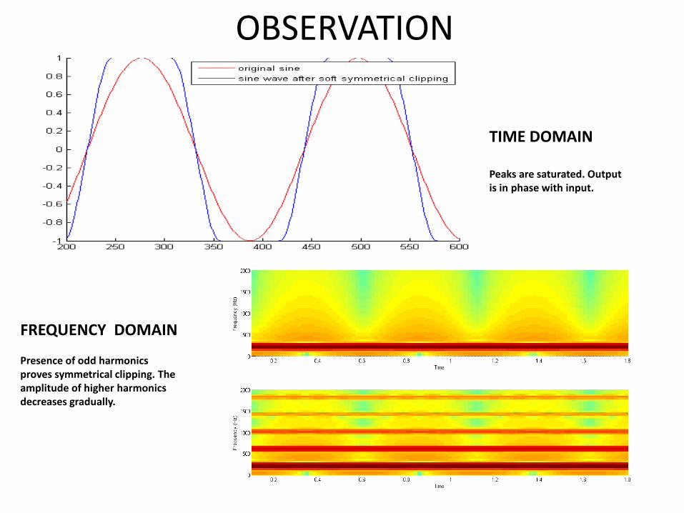
OBSERVATION

TIME DOMAIN Peaks are saturated. Output is in phase with input.

FREQUENCY DOMAIN Presence of odd harmonics proves symmetrical clipping. The amplitude of higher harmonics decreases gradually.

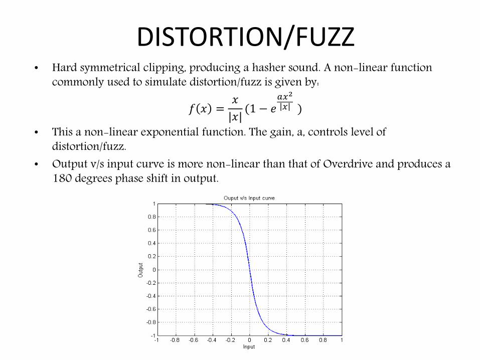
DISTORTION/FUZZ • Hard symmetrical clipping, producing a hasher sound. A non-linear function

commonly used to simulate distortion/fuzz is given by:

𝑓 𝑥 =𝑥

|𝑥|(1 − 𝑒

𝑎𝑥2

𝑥 )

• This a non-linear exponential function. The gain, a, controls level of distortion/fuzz.

• Output v/s input curve is more non-linear than that of Overdrive and produces a 180 degrees phase shift in output.

MATLAB CODE function [y] = fuzz(x, Fs)

% Distortion based on an exponential function

% x - input

% gain - amount of distortion,

% mix - mix of original and distorted sound

%1=only distorted

gain = 11;

mix = 0.1;

q=x./abs(x);

y=q.*(1-exp(gain*(q.*x)));

y=mix*y+(1-mix)*x;

end

OBSERVATION

TIME DOMAIN Hard clipping of peaks. Output is 180 degrees out of phase with the input.

FREQUENCY DOMAIN Presence of odd harmonics. Amplitude of odd harmonics greater than that of overdrive. Hence the colour of odd harmonic bands in spectrum is deeper.

WAH-WAH • A band-pass filter with time-varying resonant frequency and a small bandwidth.

Filtered signal is mixed with direct signal.

• The Wah filter can be also called a state variable filter. A state variable filter is a type of active filter. It consists of one or more integrators, connected in some feedback configuration. One configuration is such that it can produce band pass, low pass and high pass outputs from a single input.

LET’S UNDERSTAND BAND-PASS FILTERS

• A high pass filter followed by a low-pass filter gives a band pass filter.

• Centre Frequency Equation 𝑓𝑟 = (𝑓𝐿𝑥𝑓𝐻)

• Where, ƒr is the resonant or centre frequency • ƒL is the lower -3dB cut-off frequency point • ƒH is the upper -3db cut-off frequency point

FREQUENCY RESPONSE OF A SECOND ORDER BAND PASS FILTER

In case of Wah filters, the resonant frequency (f center) varies with time and the bandwitdth is small.

BLOCK DIAGRAM OF WAH FILTER

DIFFERENCE EQUATIONS: 𝑦𝑙 𝑛 = 𝐹1𝑦𝑏 𝑛 + 𝑦𝑙 𝑛 − 1 𝑦𝑏 𝑛 = 𝐹1𝑦ℎ 𝑛 + 𝑦𝑏 𝑛 − 1

𝑦ℎ 𝑛 = 𝑥 𝑛 − 𝑦𝑙 𝑛 − 1 − 𝑄1𝑦𝑏 𝑛 − 1 Where

𝐹1 = 2 sin 𝑝𝑖 ∗𝑓𝑐

𝑓𝑠

𝑄1 = 2𝑑 fc=cut off frequency, d= damping.

MATLAB CODE function [y] = wah(x, Fs) %EFFECT COEFFICIENTS % lower the damping factor the smaller the pass band damp = 0.05; % min and max centre cutoff frequency of variable bandpass filter minf=500; maxf=3000; % wah frequency, how many Hz per second are cycled through Fw = 2000; % change in centre frequency per sample (Hz) delta = Fw/Fs; % create triangle wave of centre frequency values Fc=minf:delta:maxf while(length(Fc) < length(x) ) Fc= [ Fc (maxf:-delta:minf) ]; Fc= [ Fc (minf:delta:maxf) ]; end % trim tri wave to size of input Fc = Fc(1:length(x));

% difference equation coefficients

• EXPLANATION: In the code, the center frequency (or resonant frequency) is varied as a triangle wave with values between 500Hz to 3000Hz with a step size of 2000/fs (sampling frequency is 44100Hz for all audio applications).

% must be recalculated each time Fc changes F1 = 2*sin((pi*Fc(1))/Fs); % this dictates size of the pass bands Q1 = 2*damp; yh=zeros(size(x)); % create empty out vectors yb=zeros(size(x)); yl=zeros(size(x)); % first sample, to avoid referencing of negative signals yh(1) = x(1); yb(1) = F1*yh(1); yl(1) = F1*yb(1); % apply difference equation to the sample for n=2:length(x), yh(n) = x(n) - yl(n-1) - Q1*yb(n-1); yb(n) = F1*yh(n) + yb(n-1); yl(n) = F1*yb(n) + yl(n-1); F1 = 2*sin((pi*Fc(n))/Fs); end %normalise maxyb = max(abs(yb)); yb = yb/maxyb; end

OBSERVATION

TIME DOMAIN Gradually decaying amplitude envelope indicates amplitude modulation.

FREQUENCY DOMAIN The effect of decaying amplitude also evident in spectrogram. Colour intensity of band at 200Hz decreases gradually.

TREMOLO • Modulation is the process where parameters of a sinusoidal signal (amplitude, frequency and phase) are modified or varied by an audio signal. • Amplitude Modulation (AM) is defined by: 𝑦 𝑛 = 1 + 𝑎 × 𝑚 𝑛 𝑥(𝑛) a is the modulation index. x(n) is the audio carrier signal m(n) is a low-frequency oscillator modulator. • When x(n) and m(n) both sine waves with frequencies fc and fx respectively ,we get three frequencies in the AM wave: carrier, difference and sum: fc; fc - fx; fc + fx.

• AM = (1 + a cos 2𝜋𝑓𝑥t) cos 2𝜋𝑓𝑐t

= cos 2𝜋𝑓𝑐 t +𝑎

2*cos 2𝜋 𝑓𝑐 + 𝑓𝑥 𝑡 + cos 2𝜋 𝑓𝑐 − 𝑓𝑥 𝑡+

• In tremolo, the modulation frequency is set below 20Hz.

MATLAB CODE

function [y] = tremolo(x,Fs)

index = 1:length(x);

Fx = 5; %modulation frequency

alpha = 0.5;

trem=(1+ alpha*sin(2*pi*index*(Fx/Fs)))’;

y = trem.*x;

end

TIME DOMAIN Amplitude Modulation by a modulating sine wave of low frequency is observed. The amplitude envelope varies sinusoidally.

OBSERVATION

• To observe the effect of amplitude modulation visually, in the previous code, we set Fx=1000Hz and Fc remains 200Hz;and in the spectrum, we find peaks at 200Hz,800Hz and 1200Hz.

SPECTROGRAM OF AM WAVE

FLANGER • A simple delay filter may be expressed as: 𝑦 𝑛 = 𝑎𝑥 𝑛 + 𝑏𝑥 𝑛 − 𝑀 ; where the delay is of M samples.

• In flange effect, M varies sinusoidally between 0-3ms with a frequency of 1Hz.

MATLAB CODE function [y] = flanger(x,Fs)

% parameters to vary the effect %

max_time_delay=0.003; % 3ms max delay in seconds

rate=1; %rate of flange in Hz

index=1:length(x);

% sin reference to create oscillating delay

sin_ref = (sin(2*pi*index*(rate/Fs)))';

%convert delay in ms to max delay in samples

max_samp_delay=round(max_time_delay*Fs);

% create empty output vector

y = zeros(length(x),1);

• EXPLANATION: Max_delay_dur=3ms

No of samples corresponding to 3ms=Fs*0.003=44100*0.003=132.3=132

Delay of 0.003s means delay of 132 samples

Delay will vary sinusoidally as a whole number between 0 and 132

samples.(0 to 3 ms)

% to avoid referencing of negative samples y(1:max_samp_delay)=x(1:max_samp_delay); % set amp suggested coefficient from page 71 DAFX amp=0.7; % for each sample for i = (max_samp_delay+1):length(x), cur_sin=abs(sin_ref(i)); %abs of current sin val 0-1 % generate delay from 1-max_samp_delay and ensure whole number cur_delay=ceil(cur_sin*max_samp_delay); % add delayed sample y(i) = (amp*x(i)) + amp*(x(i-cur_delay)); end end

OBSERVATION

TIME DOMAIN AM wave with modulation index>1 and modulation frequency of 2Hz.

FREQUENCY DOMAIN Intensity of frequency band at 200Hz increases and decreases alternately indicating sinusoidal modulation.

CONCLUDING…

• There are many more effects that are commonly used in guitar processors, like Reverb, Chorus, Phaser etc. Keep discovering them!

• These effects are readily available in any audio editing software like Audacity, or any DAWs like FL studio. So even if you don’t have a guitar processor, that won’t stop you from having fun with these effects!

• Now we know the signal processing that goes behind music production!There is huge scope for creating new effects. There is no end to the creativity, both musical and technical, that can be displayed in this area.

THANK YOU

REFERENCES • DAFX: Digital Audio Effects by Udo Zolzer

Copyright q 2002 John Wiley & Sons, Ltd.

• Chapter 7: Digital Audio Effects by Prof David Marshall and Dr Kirill Sidorov, Cardiff School of Computer Science.

• Multi-Effect Processor for Acoustic Guitar by Eduardo Fonseca Montero

Javier Galdon Romero, Ignacio Perez Pablos, Estrella Merino Siles, Lutz

Ehrig.

• www.electronics-tutorials.ws

• dsp.stackexchange.com

• www.wikipedia.org

• All codes written in MATLAB R2012a and audio edited in Audacity.