DiGASP Distribution Grid Analysis and Simulation with ...

Schlussbericht 23. Januar 2014

DiGASP – Distribution Grid Analysis and Simulation with Photovoltaics

2/106

D:\4868.000_Verteilte_Einspeisung_Photovol\3_Bearbeitungsdossier_1\34_Berichte und Konferenzen\2013_12 Final Report\FinalReport_Digasp_BFE.docx

2

Auftraggeber: Bundesamt für Energie BFE Forschungsprogramm Photovoltaik CH-3003 Bern www.bfe.admin.ch

Kofinanzierung: ewz AG, CH-8050 Zürich Basler & Hofmann AG, CH-8032 Zürich Austria: Austrian Research Promotion Agency (FFG) Germany: Federal Ministry for the Environment, Nature Conservation and Nuclear Safety (BMU)

Auftragnehmer: Basler & Hofmann AG Forchstrasse 395 CH-8032 Zürich www.baslerhofmann.ch

Autoren: Christof Bucher, Basler & Hofmann AG, [email protected] Jethro Betcke, Carl von Ossietzky University (Germany) Benoît Bletterie, AIT Austrian Institute of Technology GmbH (Austria)

BFE-Bereichsleiter: Dr. Stefan Oberholzer BFE-Programmleiter: Dr. Stefan Nowak BFE-Vertrags- und Projektnummer: SI/500549, SI/500549-01

Für den Inhalt und die Schlussfolgerungen ist ausschliesslich der Autor dieses Berichts verantwortlich.

http://www.bfe.admin.ch/

http://www.baslerhofmann.ch/

mailto:[email protected]

3/106


3

Table of Contents

Preface ........................................................................................................................ 6 Acknowledgement ....................................................................................................... 7 Abstract ....................................................................................................................... 8

Deutsche Kurzfassung ................................................................................................ 9 1 Introduction ........................................................................................................ 10

1.1 History of Photovoltaics ................................................................................ 10 1.2 Traditional Distribution Grid Planning ........................................................... 11 1.3 Smart Grid .................................................................................................... 12

1.4 Grid Integration of Photovoltaic Systems ..................................................... 13 1.5 Publications within this Project ..................................................................... 14

2 Problem Formulation .......................................................................................... 15

2.1 Research Questions ..................................................................................... 15 2.2 Scope of Research ....................................................................................... 15 2.3 Outside the Scope ........................................................................................ 16

2.4 Definitions .................................................................................................... 16 2.4.1 PV Penetration....................................................................................... 17 2.4.2 PV Hosting Capacity .............................................................................. 17

2.4.3 Standard Test Conditions (STC) ............................................................ 17 2.4.4 Kilowatt-peak (kWp) ............................................................................... 17

2.4.5 APC ratio ............................................................................................... 17 3 Temporal Simulation Resolution ........................................................................ 18

3.1 Objective ...................................................................................................... 18

3.2 Background of Temporal Resolutions .......................................................... 18 3.3 Data Source to Investigate Effects of Variable Temporal Resolution ........... 19

3.4 Methodology ................................................................................................. 19 3.4.1 Data Aggregation ................................................................................... 20

3.4.2 Variation of Temporal Resolution........................................................... 20

3.4.3 Voltage Calculation ................................................................................ 20 3.4.4 Power Percentile Calculation ................................................................. 21 3.4.5 Curtailed Load and Curtailed Solar Energy ........................................... 21

3.5 Results ......................................................................................................... 22 3.5.1 Voltage Drop and Rise ........................................................................... 22

3.5.2 Power Percentiles .................................................................................. 23 3.5.3 Curtailed Load and Curtailed Solar Energy ........................................... 24

3.6 Interpretation ................................................................................................ 25 3.6.1 Interpretation of Typical Timescales ...................................................... 26

3.7 Temporal Resolution in DiGASP .................................................................. 27

4 Models and Methods .......................................................................................... 28 4.1 Introduction .................................................................................................. 28

4.2 Framework ................................................................................................... 28 4.2.1 Simulation Acceleration Using Voltage Sensitivity Matrix (VSM) ........... 29

4.3 Data Sources ............................................................................................... 30 4.3.1 Load Profiles .......................................................................................... 30 4.3.2 Irradiance Data ...................................................................................... 30

4.4 Load Profile Generator ................................................................................. 30 4.4.1 Overview ................................................................................................ 31

4/106


4

4.4.2 Domestic Load Pattern .......................................................................... 32 4.4.3 Statistical Analysis of Load Pattern ........................................................ 32

4.4.4 Generation of Load Profiles ................................................................... 36 4.4.5 Validation ............................................................................................... 37 4.4.6 Use of the Load Profile Generator in DiGASP ....................................... 38

4.5 Meteo Data Generator .................................................................................. 38

4.5.1 Introduction to the Irradiance Generator ................................................ 38 4.5.2 Irradiance Generator .............................................................................. 39 4.5.3 Generator for Wind- and Temperature Data .......................................... 41

4.6 Monte Carlo Simulation ................................................................................ 41 4.6.1 Problem Formulation ............................................................................. 41

4.6.2 Required Number of Simulations ........................................................... 41 4.6.3 Limitations ............................................................................................. 42

5 Control Algorithms .............................................................................................. 43 5.1 DACHCZ ...................................................................................................... 43 5.2 Correlation with Load ................................................................................... 43

5.3 Reactive Power Control (RPC) ..................................................................... 43 5.4 Active Power Curtailment (APC) .................................................................. 44

5.4.1 Constant APC ........................................................................................ 44 5.4.2 Smart APC ............................................................................................. 44 5.4.3 Droop-based APC .................................................................................. 45 5.4.4 Stability Issues with Droop-based APC ................................................. 45

5.4.5 Optimised APC ...................................................................................... 45 5.5 Different Orientations of PV Systems ........................................................... 45

5.6 Storage ......................................................................................................... 46 5.7 Demand Side Management (DSM) .............................................................. 46 5.8 On Load Tap Change Transformer (OLTC) ................................................. 46

6 Simulation Results and Interpretation ................................................................ 47 6.1 Lumped Model ............................................................................................. 47

6.1.1 DACHCZ ................................................................................................ 48 6.1.2 Correlation with Load ............................................................................. 49

6.1.3 Reactive Power Control (RPC) .............................................................. 50 6.1.4 Active Power Curtailment (APC) ............................................................ 51 6.1.5 Different Orientations of PV Systems .................................................... 55 6.1.6 Storage .................................................................................................. 58

6.1.7 Demand Side Management (DSM) ........................................................ 60 6.1.8 On Load Tap Change Transformer (OLTC) ........................................... 63

6.2 Radial Network ............................................................................................. 64 6.2.1 DACHCZ ................................................................................................ 64 6.2.2 Correlation with Load ............................................................................. 64

6.2.3 Reactive Power Control (RPC) .............................................................. 66 6.2.4 Active Power Curtailment (APC) ............................................................ 67 6.2.5 Different Orientations of PV Systems .................................................... 68

6.2.6 Storage .................................................................................................. 70 6.2.7 Demand Side Management (DSM) ........................................................ 70 6.2.8 On Load Tap Change Transformer (OLTC) ........................................... 70

6.3 Case Study "Luchswiesenstrasse" ............................................................... 72

6.3.1 DACHCZ ................................................................................................ 73 6.3.2 Correlation with Load ............................................................................. 76 6.3.3 Reactive Power Control (RPC) .............................................................. 80

6.3.4 Active Power Curtailment (APC) ............................................................ 81

5/106


5

6.3.5 Different Orientations of PV Systems .................................................... 82 6.3.6 Storage .................................................................................................. 82

6.3.7 Demand Side Management (DSM) ........................................................ 82 6.3.8 On Load Tap Change Transformer (OLTC) ........................................... 82

6.4 Monte Carlo Results ..................................................................................... 84 7 Conclusion ......................................................................................................... 87

8 Outlook ............................................................................................................... 88 8.1 Measurement and Analysis of Load Patterns ............................................... 88 8.2 Dissertation .................................................................................................. 88 8.3 Further Research ......................................................................................... 88

9 References ......................................................................................................... 89

9.1 Papers and Reports Published within this Project ........................................ 89 9.2 General References ..................................................................................... 89 9.3 Dissemination: Presentations and Articles Hold and Published by Christof Bucher ................................................................................................................... 92

Appendix ................................................................................................................... 94

A: Optimised APC .................................................................................................. 94 B: Combination of Smart APC and Different Module Orientations and Tilt Angles 98

C: Self Consumption Ratio for Different Module Orientations .............................. 101 D: Self Sufficiency Ratio for Different Module Orientations .................................. 104

6/106


6

Preface

When this project was in preparation in the beginning of 2010, Germany just celebrated 10 GWp of installed PV capacity. Switzerland and Austria were still far away from 100 MWp each, and the Spanish PV boom was already over. The "50.2 Hertz problem" – the fact that all PV power plants in Germany (and probably in the rest of the UCTE grid) had to switch off immediately if the grid frequency should rise above 50.2 Hertz and thereby most probably provoke a UCTE-wide blackout – was already built in and identified, but the remedy against it had not been found yet.

Many scientific and industrial papers that explained how to integrate more PV power systems into the grid were published. The inverter manufacturers reacted quickly and implemented a broad variety of functionality into their devices, allowing owners of PV power plants many fancy operation modes. But the grid operators were not ready yet. Their job seemed to be by far more difficult, as they were forced to change their grids completely without knowing where the future was going to take them. Thinking rather in decades than in years, grid operators of course hesitated to install a couple of iPhones in every substation to make their grid look smart.

In this environment, the idea of "DiGASP" was born. A simulation method should be found which was able to bring all possible approaches to increase the PV hosting capacity of a distribution grid together and to compare them. In a few simple tables or graphs, the authors wanted to show the benefits of various grid integration measures, always keeping the grid in the main focus.

Today – almost four years later – the 50.2 Hertz problem has almost been solved and the first methods to increase the PV hosting capacity of a grid are being implemented in the grid codes of Germany. But there's still the same uncertainty about how the grid is going to develop, and neither the grid operators nor the operators of PV power plants really know how to integrate all solar energy into the grid. This project will not solve all these problems and uncertainties. But it will show and give both qualitative and quantitative answers to the question "How much PV can be integrated into the low voltage distribution grid?" and "How can these limitations be mitigated or removed?"

7/106


7

Acknowledgement

The authors would like to thank the PV ERA NET organisation for having brought experts from different countries together. Thanks to this network, knowledge was shared between institutions of different countries, and many synergies could be drawn on.

This project could only be undertaken thanks to funding by the national funding agencies of Switzerland, Germany and Austria. A special thanks to Dr Stefan Nowak from the Swiss Federal Office of Energy (SFOE), who not only supported the project in his administrative capacity, but also joined every general project meeting and gave his valuable feedback.

The authors would also like to thank the ewz (Elektrizitätswerk der Stadt Zürich) and especially Hansruedi Luternauer and Dr Lukas Küng for their wide-ranging support and access to the data of the distribution grid of the city of Zürich. Performing realistic grid simulations, the access to grid and measurement data is often critical. The ewz spared no effort in finding a solution to provide the data which was requested: This was not always an easy task given the confidentiality requirements on much of the information.

The scientific support of the project was provided by Dr Göran Andersson and his team of doctoral students. A big thank you for all the support they have given during the course of the project.

Last but not least I would like to thank Peter Darlington, who corrected the spelling and grammar of all the publications of DiGASP including this final report and made sure that proper British English language was applied.

8/106


8

Abstract

The PV hosting capacity of a low voltage distribution grid is investigated in detail in this project. A simulation framework is set up in order to simulate various methods and approaches to increase the PV hosting capacity of a distribution grid. The simulation approach is mainly based on two algorithms: The first algorithm generates stochastic household load profiles and the second generates stochastic irradiance data, both using a sampling rate of one to five minutes for most simulations. Applying this data to an electrical power distribution grid containing a significant number of photovoltaic systems, realistic power flow and system voltage scenarios are obtained. The results are used to precisely answer a broad range of questions concerning grid integration of photovoltaic systems.

The main purpose of this simulation framework is to find the maximum photovoltaic power which can be installed in a given distribution grid and to evaluate different measures to raise this limit. These methods consider 1) state of the art grid connection 2) correlation between load and PV 3) use of reactive power control 4) active power curtailment 5) orientation change of PV power systems 6) application of decentralised storage, 7) demand side management and 8) on load tap changing transformers.

These methods are applied to three network cases: First to a lumped load and PV model consisting of one line and one load and PV cluster. In a second step, this model is extended to a radial feeder consisting of ten network nodes, and finally the simulation approach is tested in a case study using part of the distribution power grid of the city of Zurich.

In the results of this project, it is shown that the PV hosting capacity of a distribution power grid can be increased significantly using the investigated methods and measures. The "costs and benefits" of every method in terms of technical impacts on the PV power plants and the grid are quantified.

9/106


9

Deutsche Kurzfassung

Photovoltaikanlagen (PV-Anlagen) im Netzverbund haben seit der Jahrtausendwende weltweit ein beispielloses Marktwachstum erfahren. Die elektrischen Netze wie auch die Normengebung für die Anschlussbedingungen von PV-Anlagen in den Netzen konnten mit diesem Wachstum nicht Schritt halten. Einer der Gründe dafür ist, dass viele technische Fragen in diesem Gebiet noch nicht zufriedenstellend beantwortet sind.

"Wie viel Photovoltaik verträgt ein Verteilnetz" ist die zentrale Frage dieses Projekts. Der Fokus liegt dabei auf Niederspannungs-Verteilnetzen (Netzebene 6 und 7) in sowohl städtischen wie auch ländlichen Wohngebieten der Schweiz. Alle in diesem Projekt verwendeten Methoden und Modelle werden jedoch anhand von allgemeinen Netzstrukturen eingeführt und validiert, so dass die Resultate den Anspruch auf Allgemeingültigkeit innerhalb des jeweils vorgestellten Scopes erheben dürfen.

Dieser Schlussbericht besteht inhaltlich aus zwei Hauptteilen: Im Kapitel 4 werden die Methoden der Simulationen vorgestellt, im Kapitel 6 die Resultate der Simulationen.

Das im Kapitel 4.2 vorgestellte Simulationsmodell bildet die Basis der Methodik dieses Projekts. Es besteht aus einem Lastprofilgenerator zur realistischen Nachbildung von Haushaltslasten und einem Meteodatengenrator, welcher stochastische Einstrahlungs-, Wind- und Temperaturzeitreihen für einen Standort generiert. In einem auf MATLAB basierenden Framework werden die Meteodaten zu Leistungsdaten von PV-Anlagen umgerechnet und mit den generierten Haushaltslastprofilen sowie vorgegebenen Netzdaten in der AC-Lastflussberechnung von MATPOWER ausgewertet.

Der zweite Hauptteil (Kapitel 6) besteht aus Resultaten, welche durch die Anwendung des Simulationsmodells auf verschiedene Netze und PV-Regelungsalgorithmen generiert werden. Verschiedene Berechnungsmethoden und Regelungsalgorithmen zur Bestimmung der Aufnahmekapazität von Photovoltaik im Verteilnetz werden anhand von drei Netztypen ausgewertet. Es sind dies:

Die herkömmlichen Anschlussbedingungen nach DACHCZ

Berücksichtigung der Korrelation zwischen PV und Haushaltslasten

Blindleistungsregelung

Wirkleistungsreduktion

Unterschiedliche Neigungen und Ausrichtungen der PV-Module

Lastmanagement

Dezentrale Speicher

Stufentransformatoren

10/106


10

1 Introduction

1.1 History of Photovoltaics

When Alexandre Becquerel 1839 observed the influence of light on the electric behaviour of an electrode in an electrolyte, he had not established the transformation of light energy to electrical energy. Only in 1876 did William Adams and Richard Day demonstrate the first solar cell, based on solid selenium. Inspired by their publication, research started on photovoltaic cells.

In the early 20th century, Albert Einstein theoretically explained the photoelectric effect, for which he was awarded the Nobel Prize in 1921. Various discoveries and research successes were achieved in the coming years, but no industrial product could be built until the Bell Laboratories produced the first crystalline silicon solar cells in the early 1950's with an efficiency of 4 %.

The first real applications, and the driving force for the development of solar cells in the coming decades, were in the space industry. In 1958 the first US satellite equipped with batteries and solar cells was sent to space. Up to today, almost all satellites take their energy from solar cells.

Fig. 1: Evolution of global PV cumulative installed capacity 2000-2012 (MW). Source: EPIA Global Market Outlook [7].

For a long time, space technology remained the main area of application for PV, until the oil crisis in 1973 provoked a global change of thinking and the use of photovoltaic systems for terrestrial electricity supply was discussed seriously for the first time. By the mid-seventies various research facilities were committed to improving the efficiency of solar panels. During

11/106


11

the eighties and nineties the efficiency of photovoltaic cells was raised from less than 10 % to around 16 %.

In the early nineties the first national funding programs started to appear, providing financial incentives for people willing to install solar power. These programs marked the beginning of the commercial use and trade in photovoltaics. In the year 2000 the PV market started to grow more rapidly thanks to the incentives mentioned and to increasingly lower module prices.

In 2005 Spain approved a new national energy plan along with other European governments. The aim of this plan was to increase renewable energy production to 30 % of the country's overall energy consumption by 2010. To reach these targets the government supported each technology with substantial incentives. In case of photovoltaics this meant a feed in tariff of 43 to 45 Eurocents or 8-10 times more than the average market price for conventional power. These circumstances lead to a dramatic increase of PV Installations. In 2007 the government realized that they were about to overshoot their target and devised new regulations to reduce feed in tariffs by the end of 2008. This lead to an even greater run on PV installations with 2'500 MW capacity installed in 2008, more than 100 times the amount installed in 2005. At this point Spain accounted for 43 % of the global PV market. Following the reduction of the feed in tariffs the local PV market in Spain collapsed and the installation capacity was reduced to a maximum of 500MW per year.

In 2009 Germany replaced Spain as the leading market in Europe but overall growth was limited. In general investments were roughly in line with consumer demand until 2009. Thanks to constant growth of the PV market, many new manufacturers started to appear and simultaneously companies started expanding their production capacity. This led to a huge increase in spending during 2010 and 2011. In 2010, in Germany, Italy and the Czech Republic, installation increased the cumulative installed capacity by a factor of 2. Just as in the Spanish market, the Czech Market collapsed in the following year, but the German and Italian market continued to grow.

By the end of 2011, production capacities had been raised to 60 GW which exceeded the predicted market volume for 2012 by a factor of 2. Combined with other changes in the solar market such as the revised EEG in Germany, the market in the PV book-to-bill ratio turned negative in the first half of 2012 indicating a downturn of the industry.

Prices of modules fell to an all-time low which left manufacturers having to produce products with cash-costs exceeding sales prices. Inevitably many PV companies became insolvent [8].

1.2 Traditional Distribution Grid Planning

Today's high voltage transmission grids could not be operated safely if they could not be simulated using power flow computation, state estimation and further grid simulation methods. Up until today, this has not been necessary for distribution grids. Issues which are handled in the distribution grid planning are [9]:

Estimation of energy demand

Connection to high and medium voltage grid

Low voltage distribution

12/106


12

Protection against electric shocks

Protection of devices in the low voltage grid

Voltage surge protection

Power factor correction, reactive power

Harmonics, flickering

Special power sources and loads

Electromagnetic compatibility (EMC)

Distribution grids are traditionally planned as unidirectional: Power flows only from the higher voltage levels to the loads. Voltage drops are assumed from the transformer to the loads, therefore the transformer voltage is set slightly above to maintain a reasonably high voltage at the load.

Having an estimation of the demand (both energy and power consumption characteristics), the electrical equipment is chosen using diversity factors, coincidence factors and further tabulated design criteria.

However, the coincidence or correlation between PV and loads is neglected by these traditional methods. This is an element which will be investigated in detail in this project. Furthermore, modern photovoltaic power inverters offer a wide range of grid integration options, which are not covered in traditional distribution grid planning.

1.3 Smart Grid

"Smart grids are nothing new. We have always had smart grids, just not on the distribution level." (small talk with Prof. Göran Andersson, 2010)

Smart grid technology has been implemented in domestic installations since 1960 but was not common until 1990. Today modern building automation systems rely on a network of various household appliances communicating with each other. By continuously measuring different parameters and communication with controllers the system can optimize energy use and turn off redundant appliances. The basic idea of a smart grid on distribution level relies on a similar principle to that applied to building automation systems.

Most of the electricity grid throughout Europe is based on technology that was developed more than 30 years ago. Even today most of the energy we consume is produced in large centralized power plants and distributed by a one way energy grid. Up until now this outdated system has been able to maintain its position as the method of operation. In recent years however, the conventional power grid has been faced with new challenges which have put electricity networks under pressure to change [10].

There are three main driving forces that are forcing energy suppliers to rethink their method of distribution. The most common factor is the increasing number of decentralized power plants that are connected to the grid. To maintain grid stability the grid operators need to know which plant produces which amount of energy. To achieve this, a communication network between the decentralized power plants and the grid operator is necessary.

13/106


13

Simultaneously, the number of intermittent renewable energy sources connected to the grid has also been rising. Contrary to base load power sources, these power sources have a fluctuating output. The most common intermittent energy sources are photovoltaics and wind energy. The output of these sources is dependent on the local weather and can therefore influence the amount of energy produced.

The final main factor is the EU Energy and Climate Package which has set various targets for 2020. In short the aim is to reduce greenhouse gas emissions, increase the share of renewable energy sources and reduce primary energy consumption. All these targets will influence the way energy is produced, distributed und consumed.

A smart grid consists of an electrical grid with additional sensors to gather information on grid conditions such as energy production and consumption. The gathering of this information is essential since energy demand must be equivalent to energy production at any time to guarantee grid stability. There are various methods to regulate grid stability. Through demand side management, grid operators are able to turn off certain loads on the demand side to reduce and shift peak demand. Flexible price structures as used in a demand response scheme are set to reduce the customer's consumption during high load periods.

Thanks to the permanent surveillance of the grid, the loads and the energy production of all those involved can interact with each other and regulating measures can be taken. This allows for an energy efficient system that is able to handle fluctuating energy sources whilst maintaining grid stability [11].

1.4 Grid Integration of Photovoltaic Systems

When distribution grids were first built, their task was simple: To receive electrical power from a central feeder and to deliver it to distributed loads. With the increasing share of distributed generation (DG) and particularly photovoltaics, power flow started to invert at certain points in time. This caused directly some new challenges, e.g. in the fields of voltage control and protection.

The first reaction of the utilities was to limit the maximum PV power in the grid to a limit lower than the permitted load power. This impeded in many cases the realisation of PV power plants on rooftops.

To mitigate this limitation, the European Photovoltaic Industries Association (EPIA) collected a list of 14 measures to increase the share of PV in the transmission and distribution grid [13]:

1. Enhanced fault ride through capability

2. Enhanced inverters with short circuit power output

3. Frequency dependent power reduction

4. Improved feed-in prognosis

5. Stepwise power reduction*

6. 3-phase grid connection

7. Voltage VAr control at PV converter*

8. MV/LV on load tap changer*

14/106


14

9. MV/MV or LV/LV booster transformer

10. Voltage control at customer connection

11. Demand response*

12. “Classic” network reinforcement

13. Storage (central)

14. Storage (distributed)*

The measures marked with an asterisk (*) plus the correlation between PV and load and the analysis of different orientations of PV modules will be discussed in this project.

1.5 Publications within this Project

Four papers and two technical reports where published within this project. The full references are given in chapter 9.1.

Generation of Domestic Load Profiles – an Adaptive Top-Down Approach [1].

Simulation of Distribution Grids with Photovoltaics by Means of Stochastic Load Profiles and Irradiance Data [2].

Effects of Variation of Temporal Resolution on Domestic Power and Solar Irradiance Measurements [3].

Increasing the PV Hosting Capacity of Distribution Power Grids – a Comparison of Seven Methods [4].

Development and Validation of the DiGASP Weather Generator, Technical report [5].

Implementation of local voltage control by PV inverters in LV networks – Considerations on the parameterisation and stability issues, Technical Report [6].

15/106


15

2 Problem Formulation

2.1 Research Questions

The central research question of this project is: "How much PV can be integrated into the low voltage distribution power system?" This question will be answered not only using the current practice in grid connection technologies, but also using several available technologies to increase the PV hosting capacity of a low voltage grid.

Today, a broad range of grid integration measures for PV power systems is known and is partly available on the market (chapter 5). It is a major goal of this project to evaluate several of these measures and to compare their performance based on one uniform simulation environment in order to obtain consistent results.

The results produced in this project should end up in new "rules of thumb", tables and graphs to estimate the PV hosting capacity of a distribution grid and the benefit of a specific grid integration measure. It is of course not possible to calculate the PV hosting capacity and the impact of a certain measure on any specific low voltage distribution grid only out of the results of this project, but it will be possible to make an estimation about what effects could be expected and which further investigations should be made.

Alongside these quantitative answers to "what-if-questions", the distribution of worst case situations is investigated. For optimised grid design, it is important to know whether a critical situation occurs once a day or only once in a year. By means of Monte Carlo simulations, such questions will be answered.

2.2 Scope of Research

This project investigates the low voltage distribution grid and the connected transformer (grid level 6 and 7, see Fig. 2). The main focus is therefore on the grid voltage, but also the current loading is investigated. The grid at the medium voltage side of the transformer (grid level 6) is modelled as a constant voltage feeder.

Within grid level 6 and 7, domestic household loads and PV power plants are modelled and simulated. Correlation between these loads and PV is studied in detail. In the case study, beside the domestic household loads, certain assumptions for industrial loads are made, without however modelling them in detail. All loads and PV power plants are modelled symmetrically on three phases, asymmetries are neglected.

To simulate PV power plants, various control algorithms are used. They are taken from previous publications and are sometimes slightly modified. Algorithms for reactive power control and active power curtailment are studied in considerable detail, whereas demand side management for example is only treated superficially using rough estimations regarding its potential.

16/106


16

Fig. 2: Traditional electricity transport trough seven grid levels. Source: Swissgrid [14]

2.3 Outside the Scope

As the medium voltage is modelled as a constant voltage feeder, system wide aspects such as frequency and energy balances do not fall within the scope of this project. If a rainy summer fills all the water reservoirs and therefore compensates for bad solar energy yield, this does therefore not affect the simulation results.

Concerning power quality, only the steady state voltage is analysed. Other power quality aspects such as flicker, harmonics, transients or phase asymmetries which are not inherently coupled with PV power in the grid, are not investigated.

Many control algorithms are used in this project. To fit them into the simulation framework some adaptions and optimisations are made. It is however outside the scope of this project to implement new control algorithms.

2.4 Definitions

Most terms used in this report are well defined, normally by a standardisation organisation such as ISO1 or BIPM2. However, some terms are used inconsistently in literature or lack an official definition and will therefore be defined in the following sections. Even terms which are very specific and might not be known by the reader are defined here, e.g. "Standard Test Conditions".

1 ISO: International Organisation for Standardisation

2 BIPM: Bureau international des poids et mesures, the International Bureau of Weights and Measures

17/106


17

2.4.1 PV Penetration

The "PV penetration" of grid A is defined as the yearly solar energy fed into grid A divided by the yearly energy consumption of all consumers connected to grid A. A PV penetration of 100 % in a rural grid results therefore normally in a PV peak power which is higher than peak load.

2.4.2 PV Hosting Capacity

The "PV hosting capacity" is the maximum PV penetration at which no technical or legal constraints in the grid are violated. If not explicitly mentioned, the relevant constraint to be fulfilled is to keep the maximum voltage rise limited to 3 %.

2.4.3 Standard Test Conditions (STC)

STC are the conditions under which a solar cell and a PV module are tested in the laboratory. The STC test results are used as the primary information to characterise a PV module. STC are defined as follows:

Irradiance of ⁄

Cell Temperature of

Air Mass of

This corresponds roughly to the ideal conditions a module could face in operation.

2.4.4 Kilowatt-peak (kWp)

Kilowatt-peak has become a standard term in recent years. It is normally used as a unit, which according to SI definitions is not correct. However, one kilowatt-peak is defined here (in accordance with the vernacular) as the number of PV modules which have a power output of one kilowatt under standard test conditions.

2.4.5 APC ratio

The APC ratio (ratio of active power curtailment) is defined as the nominal inverter power divided by the nominal DC power (in kWp) of the PV modules:

18/106


18

3 Temporal Simulation Resolution

3.1 Objective

In order to study power flow and voltage stability in a distribution power grid, it is obvious that a temporal resolution of one hour is not sufficient. Clearly, it will not be possible to perform long term simulations with a temporal resolution of one second or less, as too much computational power would be required. The objective of this chapter is therefore to find an appropriate temporal resolution for the DiGASP simulations.

The higher the temporal resolution of a simulation, the more accurate are the results. An optimum trade-off is however needed in order to minimize the computational power. This optimum turns out to be between one and five minutes.

Once this optimum of one to five minutes is given, estimation of the accuracy loss should be made. The investigations and results in this chapter provide a base for such an estimation.

3.2 Background of Temporal Resolutions

Different metering purposes in electric power grids require different temporal resolutions. Billing of domestic electricity consumption is traditionally based on annual meter values. Electric energy trading is normally done on a one hour basis, whereas electricity metering for large customers is done on a 15 minute basis [15]. Due to the large requirement for data storage and expensive measuring equipment, the availability of measurements with a temporal resolution of less than 15 minutes is poor. The measurement data used in this report is presented in chapter 4.3.

In previous studies, the temporal resolution of measurement data has already been analysed. Wright et al. [17] consider five minute values to be insufficient, but do not look beyond one minute measurement data. Furthermore the consequences of excessively low temporal resolution are not studied in detail. Widén et al. [18] compare ten-minute and one-hour data aggregation for domestic load measurements and photovoltaic power plants, concluding that hourly data is sufficient for voltage rise investigations.

The specifications of the voltage characteristics of electricity supplied by public distribution networks are defined in EN 50160:2010 [19]. In accordance with section 4.2.2.2 of EN 50160, the voltage in the distribution grid must be within the limits of ±10 % for 95 % of the time based on mean 10 minute rms values over a week.

In this chapter, the ratio of calculated voltages applying different temporal resolutions is analysed. Voltage rise and drop caused by distributed photovoltaic systems and domestic loads are compared. Theoretical values of curtailed load (CL) and curtailed solar energy (CSE) due to voltage violations are calculated. Whenever household loads and solar irradiance are to be represented realistically in terms of maximum power, maximum voltage and energy flows, a temporal resolution of one minute is proposed for simulation purposes.

However, this does not apply to the analysis of transient currents and voltages in the grid, where much higher temporal resolutions are required. In contrast, the proposed temporal resolution might be too high if only a broad overview of the energy flows in a grid are to be obtained.

19/106


19

3.3 Data Source to Investigate Effects of Variable Temporal Resolution

This chapter focuses on long-term measurements with a temporal resolution of one second. The poor availability of such measurement data is assumed to be the main reason why investigations as shown here have not yet been published.

Three household measurement sets with a temporal resolution of one second and a measurement period of several days to several weeks were available for this report:

Thirty households in Austria [20]

Seven households in the USA [21]

Four households in Switzerland [22]

The horizontal global irradiance was measured with a resolution of second on the roof of Oldenburg University (3.15° N, 8.17° E) using a Kipp and Zonen CM 11 pyranometer, which was calibrated by the manufacturer in March 2010. In this investigation, measurements from the period June 2011 to April 2012 are analysed [23].

A sample of a one-day household load pattern and irradiance profile is shown in Fig. 3. Both the household load and the irradiance data are plotted in the original temporal resolution of and a reduced resolution of .

Fig. 3: Load and irradiance measurement of one summer day. Temporal resolution of 1 second and 15 minutes.

3.4 Methodology

The aim of this chapter is to find the optimum temporal resolution for representing voltage, power and energy in distribution grids with a high share of domestic households and photovoltaic power plants. Consequentely, the following three methodologies are used to analyse the data:

analysis of maximum calculated voltage

analysis of the power percentiles

analysis of energy curtailment

20/106


20

3.4.1 Data Aggregation

To investigate the effects of data aggregation, measurement data sets are merged. As only 41 household load patterns are available (see section 3.3), different days of a single household are merged into one day, if the cumulative effect of more than the available number of households is investigated.

3.4.2 Variation of Temporal Resolution

All measurement data presented in section II is available with a temporal resolution of one second. Corresponding data is aggregated in this chapter to temporal resolutions of 5 s, 15 s, 30 s, 1 min, 15 min, 30 min and 1 hr, using the arithmetic mean value of the aggregated data points.

Fig. 4: Setup of the power grid consisting of a) one feeder and one household, b) of one feeder and n households and c) one feeder and a photovoltaic power plant.

3.4.3 Voltage Calculation

Several approaches study the effects of the temporal resolution on distribution grid simulation. First the voltages in a simple power grid consisting of a feeder and one or several households (Fig. 4) are computed. The line is modelled using the π-model [24]. The voltage at the household node is calculated using (1).

(

) (

)( ) (1)

where denotes the feeder node, the household node, is the series admittance,

the shunt susceptance and the voltage.

The current from the household node towards the line can be expressed as a function of

and the complex conjugated apparent power consumption at node (2).

21/106


21

(2)

Solving (1) for the voltage at the household node , (3) is found.

√( )

( )

( )

(3)

If the shunt susceptance is neglected and the voltage at the household node is close to

the feeder voltage ( ), (3) is simplified to (4).

(4)

As the feeder voltage is kept constant, the voltage deviation at the household node is proportional to the load at the household node. This means that all voltages calculated in this chapter are essentially proportional to the power which is consumed or fed in at the given point. The results are presented as voltage deviations as a function of the temporal resolution in accordance with (5),

( ) ( )

( ) (5)

which can be simplified to (6).

( )

( )

( )

(6)

Because the reactive power consumption has only a small influence on the voltage in the low voltage grid, the complex conjugated apparent power is set to the active power

.

3.4.4 Power Percentile Calculation

A second approach used in this project to investigate the effects of different temporal resolutions on load and irradiance data is to calculate the power percentiles, as presented in Wright et al. [17]. A change in the percentiles for lower temporal resolutions indicates information loss due to the change of the temporal resolution.

3.4.5 Curtailed Load and Curtailed Solar Energy

If a given voltage tolerance band is to be respected, only limited power can be consumed or fed into the grid. In this calculation method, the line is dimensioned such that the power consumption and production independently cause voltage dips and rises of exactly 3 % if the temporal resolution is 1 hr. The curtailed load (CL) and the curtailed solar energy (CSE) are

22/106


22

the energies which cause voltage deviations beyond 3 %. Their computation is done in accordance with (7).

( ) ∑ [ ( ) ( ) ]

( )

⏟

∑ [ ( ) ( )]

( )

⏟

(7)

where

{ ( )

TR denotes the temporal resolution, ( ) the power at the time , ( ) is the total number of measurements for the given temporal resolution. Part A is the total energy demanded when a voltage violation occurs; Part B is the energy which theoretically still could be served during the voltage violation.

The tolerance of 3 % is chosen to minimise effects of line losses and to follow the dimensioning practices promoted in the D-A-CH-CZ-compendium [25].

3.5 Results

The results are presented in three sections in accordance with the methods presented in chapter 3.4:

Voltage drop and rise

Power percentiles

Curtailed load and curtailed solar energy

3.5.1 Voltage Drop and Rise

Averaging data reduces peak values and increases the minimum measured values. The measured peak power and thus the maximum expected voltage dip within one hour vary considerably depending on the temporal resolution used for the measurement. A sample

worst case scenario is given by a power impulse of during . This value can only be measured if a temporal resolution of is applied. Using a sampling rate of , the

maximum power detected would be in the same situation. Given a temporal resolution of one hour this value would decrease to the meaningless value of . The voltage

deviation computed with (6) using a temporal resolution of one hour would therefore deviate by a factor of from the real value.

Fig. 5 (a) shows the ratio of maximum voltage changes for different temporal resolutions and different numbers of aggregated households using (6). Fig. 5 (b) shows the same analysis for power fed into the grid by solar irradiance. A comparison of both graphs shows that the solar

23/106


23

irradiance data causes a similar ratio of maximum voltage changes as an aggregation of about five to ten households.

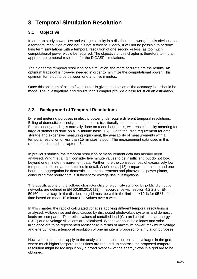
3.5.2 Power Percentiles

Fig. 6 shows different power percentiles of the measurement data. It is conspicuous that the percentile (which approximately represents peak power) drops drastically if lower temporal resolutions are applied. This means that power peaks are clipped. The obverse effect can be observed with the percentile which represents low power: If the temporal

resolution is lower than about , this percentile rises.

The comparison between household data and irradiance data again shows similarities

between a certain number of aggregated households and the irradiance data. The percentile for a single household drops about if the temporal resolution in increased

from to . The same percentile of ten households as well as of the irradiance data drops about , whereas the percentile of households only drops about . In terms of power percentile variation the irradiance data can be compared to an aggregation of ten to fifty household load patterns.

Fig. 5: Ratio of maximum voltage changes caused by household loads (a) and irradiance (b) applying different temporal resolutions, using (6).

24/106


24

Fig. 6: Percentiles of load measurement of one (a), ten (b) and two hundred (c) households given in power per household. Percentiles of irradiance data (d). The percentiles are shown as a function of the temporal resolution. Because the percentiles vary over several decades, the plots are split into three parts.

3.5.3 Curtailed Load and Curtailed Solar Energy

The line voltage of a line designed to withstand household loads with voltage deviations of less than on an hourly basis obviously deviates more than if voltage deviation

25/106


25

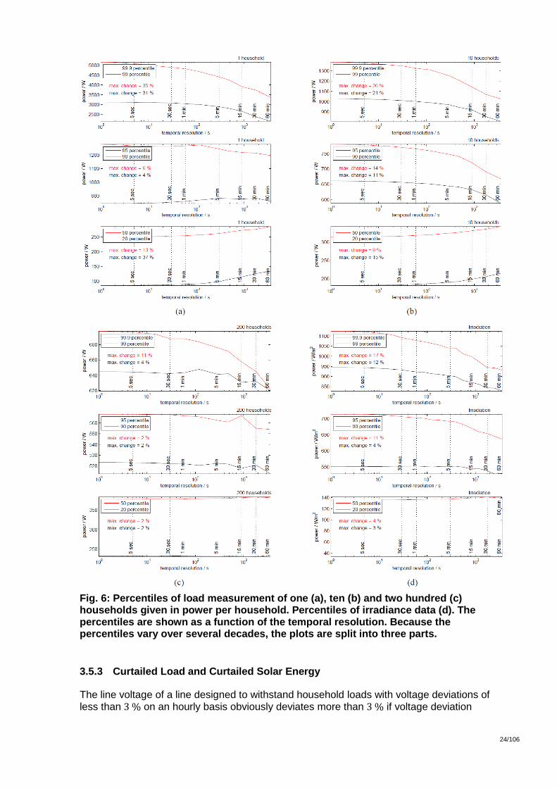
calculations with a higher temporal resolution are made (see section 3.5.1). Fig. 7 shows the percentage of CL for different numbers of households (a) and a photovoltaic power plant (b).

If only one household is connected to the grid which is designed to withstand the peak power on a one hour average basis, about of the load cannot be served. This number decreases rapidly if more households are connected to the grid. In addition, the curves representing many households are flatter than those representing only a few households. This means that the impact of excessively low temporal resolution decreases not only in absolute but also in relative values with an increasing number of households on the grid.

Fig. 7: (a) Curtailed load (CL) and (b) curtailed solar energy (CSE). This Energy has to be curtailed, if a line is designed based on TR = 1 h.

The results are not linear and depend on the household(s) investigated. Looking at the American measurement data set, CL goes up to for a single household. This means that in the given American data set, households consume more energy at peak power than in the other data sets.

The CSE reaches a maximum of if the maximum temporal resolution of one second is applied. This corresponds again to five to ten aggregated households.

Generally, the impact of a low temporal resolution on energy is much lower than on power. Nevertheless, similar characteristics can be observed in both cases.

3.6 Interpretation

The three methods presented to analyse the change of the statistical properties of domestic load and irradiance data have one common outcome: The higher the temporal resolution, the fewer the effects of temporal resolution variation.

26/106


26

Fig. 8: Weighted and normalised second derivative (differential quotient) of the three presented results and their mean value. All voltage changes, percentiles and energy curtailment curves are used. This is an objective indication for plot reversals and thus “change of changes” in the result graphs.

One approach to find the optimum resolution is to identify the major change in the results presented. Fig. 8 shows the second derivative of all three methods presented in chapter 6 with respect to the temporal resolution. It is calculated using differential quotients and the discrete temporal resolutions shown in the graph. The peak of the bold curve at and at

denotes the major bend in the result curves. This means that changing the temporal resolution stepwise from to , the highest loss of information takes place between

and . The conservative but reasonable choice is therefore to choose as the optimal temporal resolution.

3.6.1 Interpretation of Typical Timescales

The proposed temporal resolution of one minute data can be found again in the daily use of household appliances. A broad range of widely spread electrical devices consuming relatively high power are switched on and off for several minutes, but normally for not less than one minute and not longer than five to ten minutes. Such devices are:

Thermal switching electrical ovens

Toasters

Hair dryers

Electric kettles

The authors of this project assume that the use of these devices is a dominant reason for the behaviour of the measured domestic load patterns.

Similar reasoning can be applied to the solar irradiance. The minimal required temporal resolution is determined by days with scattered clouds. During such conditions, the time between clear sky - cloudy sky transitions is in the range of several minutes to an hour [26], [27].

27/106


27

3.7 Temporal Resolution in DiGASP

In this project, simulations are basically done with a temporal resolution of one or five minutes. But since one year has 525'600 minutes, a power flow computation of one year with a temporal resolution of one second needs a lot of computational power. For some repeated simulations, a lower temporal resolution is therefore chosen. The final results are in this case corrected linearly in accordance with the deviations between two test simulations, which differ only in the temporal resolution.

28/106


28

4 Models and Methods

4.1 Introduction

One objective of this project is to present or to provide a simulation platform which allows precise and efficient simulation of PV power plants in low voltage distribution grids. Such a simulation platform is presented in this chapter. It consists of the following sections:

The simulation framework

The data sources for load and irradiance modelling

The load profile generator

The meteo data generator and

The Monte Carlo Simulation approach

With the content and results of this chapter, it will be possible to perform the simulations which are necessary to answer the principal question of this project, which addresses how much PV can be integrated into a low voltage distribution power grid.

4.2 Framework

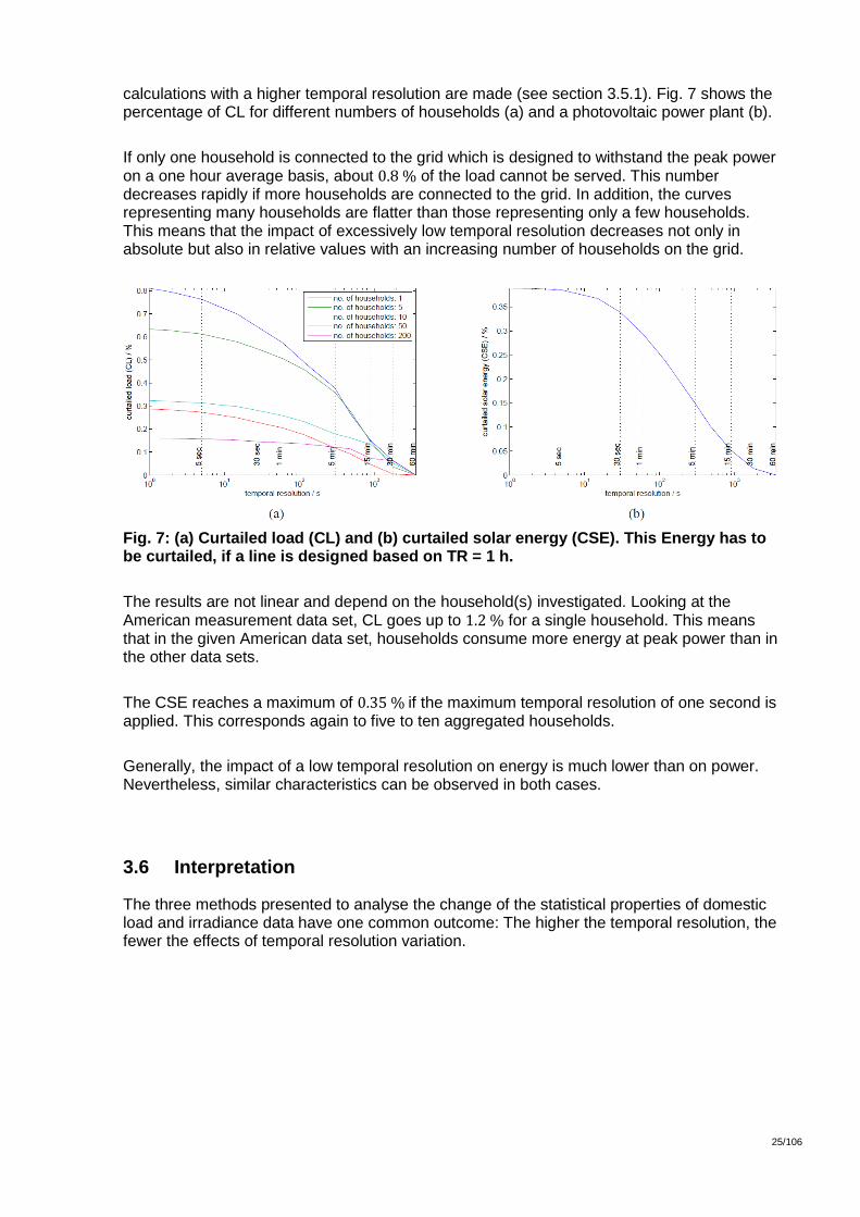
An overview of the simulation procedure is given in Fig. 9. Starting from the grid topology which contains information about households and PV power plants, the required load profiles and irradiance data are generated. The actual consumption of the households is simulated using additional information about demand side management (DSM). The maximum power output of each PV plant is computed using the irradiance profile and a reference temperature profile.

Given the power demand and the power production of every node in the grid, an AC load flow computation is performed using Matpower [28]. The nodal voltages are fed back to the active power curtailment (APC) and reactive power control (RPC) algorithm.

The modular topology of this scheme permits the enabling and disabling of different functionalities of the simulation procedure. The functionalities which are currently implemented are presented in chapter 5.

29/106


29

Fig. 9: Simulation procedure with demand side management (DSM), maximum power point tracking (MPPT), active power curtailment (APC) and reactive power control (RPC). 4.2.1 Simulation Acceleration Using Voltage Sensitivity Matrix (VSM)

In many cases, only the critical simulation times (e.g. when maximum or minimum voltages occur) are of interest. If this is the case, only a small number of time steps must be simulated. The VSM can be used to estimate voltages and make a choice of critical time steps.

The VSM consists of two symmetrical matrices VSMP and VSMQ, where denotes the number of nodes in a distribution grid (8). In the following equations, the procedure to calculate VSMP is described. VSMQ can be obtained in exactly the same way, just replacing p by q.

[

]

(8)

The coefficients of the VSM are defined as the voltage change at node , if a given

power is applied to node .

load profile

generation DSM

irradiance

generation

energy demand MPPT

power output

APC, RPC

power flow computation voltages, currents

distribution grid households, PV systems, grid topology

30/106


30

(9)

If all voltages in the system are close to , the voltage deviations are proportional to the power applied to the nodes and hence the coefficients are constant. This condition is

given in (10).

(10)

The derivation of the coefficients is done empirically in this project. A test load is applied

to every node, and the voltages are simulated using the power flow simulation tool MATPOWER.

To calculate or rather estimate the voltage at node , the voltage deviations caused by all

power fed in the grid must be summed up and added to (11).

∑

∑

(11)

Using (11), the voltages of any grid with known VSM can be estimated with only little computational power; even if the number of time steps is high (e.g. 1 minute steps during one year). The most critical time steps can then be selected and simulated using a power flow simulation tool. Especially for Monte Carlo simulations, this is a very useful way to accelerate grid simulation.

4.3 Data Sources

4.3.1 Load Profiles

The load profiles used in the simulations of this project where generated using the load profile generator of chapter 4.4. Measurements of the electricity demand of 50 households in Zurich were recorded in 2013, but they were not yet available for the simulations.

4.3.2 Irradiance Data

Irradiance data is taken from the meteo data generator presented in chapter 4.5 and from test reference years of METEONORM [29].

4.4 Load Profile Generator

The objective is to generate a load profile which can be used for distribution system power flow and voltage analysis. The algorithm should be fast and allow the generation of a large number of load profiles with only little computational power.

31/106


31

When distribution systems are simulated nowadays, household loads are normally represented with an aggregated load profile. Such an aggregated load profile is sufficiently accurate for the system as a whole, but does not represent individual households. In order to investigate the correlation between household loads and distributed power generation, high resolution household load profiles are needed. As the number of profiles needed is large, the algorithm to generate them must be fast.

It is not of interest whether a certain appliance is used at a certain time, but the overall power demand of a household must be realistic. The following statistical criteria must therefore be met:

The load distribution function (load histogram) at any time

The mean load duration of any load at any time

The sum of a large number of load profiles must correspond to a given reference load profile.

It must be possible easily to generate a large number of load profiles.

The generated power factor ( ) must statistically correspond to the measured power factor for every load at any time.

Excluded from the criteria to be met are auto-correlations within a single load profile. They are typically produced by thermal switching loads such as fridges and freezers, but also by stoves and ovens.

4.4.1 Overview

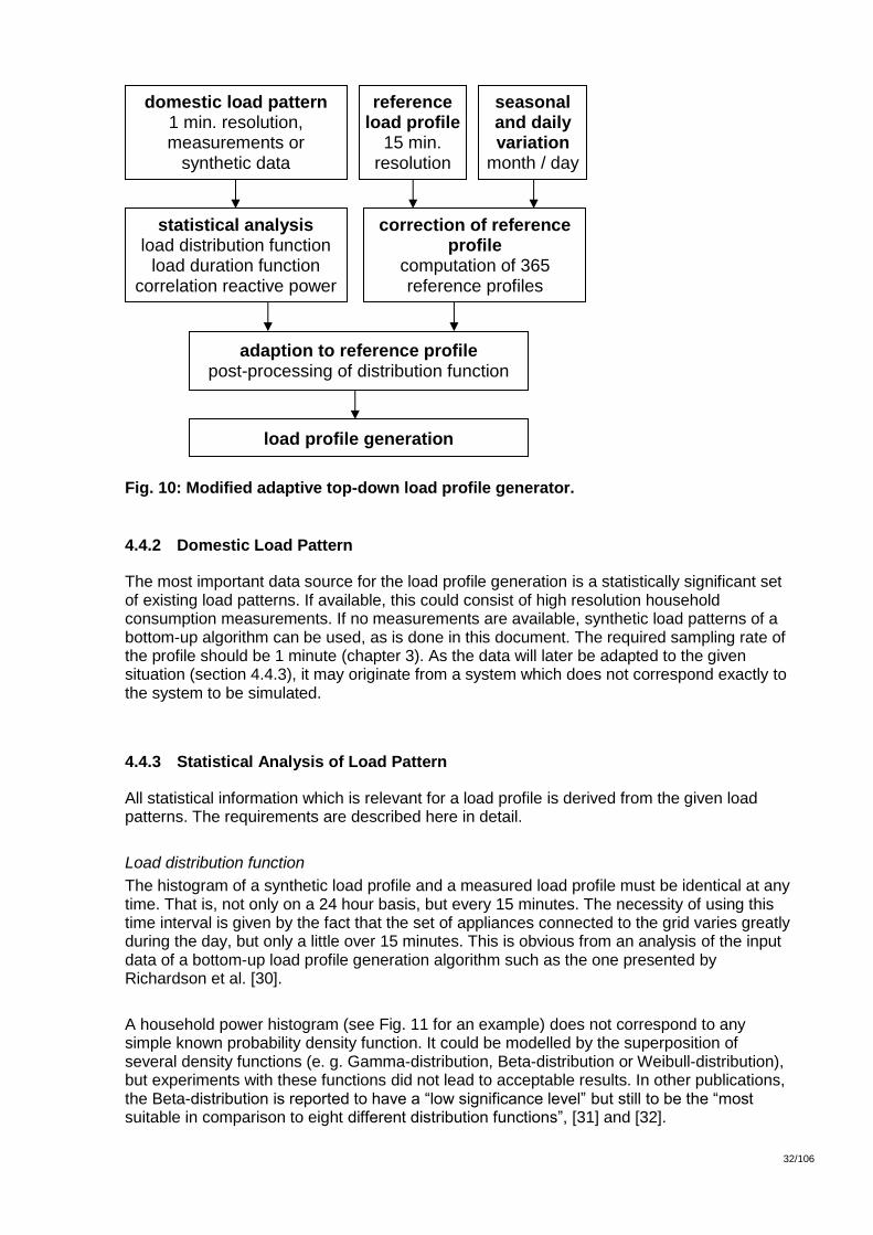
The load patterns which are statistically analysed are generated with the bottom-up algorithm presented by Richardson et al. [58]. As this algorithm is based on consumer data from the UK, a few configuration modifications are made to obtain results close to continental European electricity consumption patterns. The main steps of the top-down load profile generation algorithm presented in this document are shown in Fig. 10. In the following sections, these steps are described in detail.

32/106


32

Fig. 10: Modified adaptive top-down load profile generator.

4.4.2 Domestic Load Pattern

The most important data source for the load profile generation is a statistically significant set of existing load patterns. If available, this could consist of high resolution household consumption measurements. If no measurements are available, synthetic load patterns of a bottom-up algorithm can be used, as is done in this document. The required sampling rate of the profile should be 1 minute (chapter 3). As the data will later be adapted to the given situation (section 4.4.3), it may originate from a system which does not correspond exactly to the system to be simulated.

4.4.3 Statistical Analysis of Load Pattern

All statistical information which is relevant for a load profile is derived from the given load patterns. The requirements are described here in detail.

Load distribution function

The histogram of a synthetic load profile and a measured load profile must be identical at any time. That is, not only on a 24 hour basis, but every 15 minutes. The necessity of using this time interval is given by the fact that the set of appliances connected to the grid varies greatly during the day, but only a little over 15 minutes. This is obvious from an analysis of the input data of a bottom-up load profile generation algorithm such as the one presented by Richardson et al. [30].

A household power histogram (see Fig. 11 for an example) does not correspond to any simple known probability density function. It could be modelled by the superposition of several density functions (e. g. Gamma-distribution, Beta-distribution or Weibull-distribution), but experiments with these functions did not lead to acceptable results. In other publications, the Beta-distribution is reported to have a “low significance level” but still to be the “most suitable in comparison to eight different distribution functions”, [31] and [32].

domestic load pattern 1 min. resolution, measurements or

synthetic data

reference load profile

15 min. resolution

statistical analysis load distribution function

load duration function correlation reactive power

adaption to reference profile post-processing of distribution function

load profile generation

seasonal and daily variation

month / day

correction of reference profile

computation of 365 reference profiles

33/106


33

Integrating and normalising the household power histogram leads to the cumulative distribution function (CDF).

( )

∫ ( )

(12)

where is the number of measurements in the histogram (Fig. 11), is the household power (x-axis in the histogram) and ( ) the absolute frequency of the household power measurements.

The distribution of the household power is modelled with a set of linear functions, each modelling one segment of the CDF. The sampling points for these linear functions are derived by putting all power measurements of in a strictly monotonic increasing row. This row is approximated with 20 sampling points chosen on a logarithmic power scale.

Fig. 11: Household power histogram for time span 8 pm to 8:15 pm.

Fig. 12: Stepwise linear cumulative distribution functions (CDF) for 2 am and 8 pm (red), based on the histogram in Fig. 3 and Eq. 1 (blue).

Fig. 12 shows two sample CDFs, generated for and . The CDFs are based on

generated power samples from to and to . Both time intervals are represented by power samples.

The stepwise linear CDFs (red in Fig. 12) can be described with pairs of power Pi and its corresponding cumulative probability ( ) where denotes the power segment and the

time. The load sectors are defined in logarithmically distributed steps, using the following Matlab command:

load_sector = logspace(log10(Pmin), log10(Pmax),21)

34/106


34

The data to be stored for the load profile generation algorithm consists therefore of pairs

of ( ( )⁄ ) for every , this demands a matrix with the dimension of . The

construction of the matrix is shown in (13).

[

]

(13)

As is time independent, it must not be stored in every row. For improved understanding, this is nevertheless done.

To generate a load profile, for each sampling time a uniformly distributed random variable ( ) is selected. With the CDF in Fig. 12 (equivalent to the matrix in (13)) the

corresponding household power is calculated. Although there is only one CDF for , power samples can be drawn with any arbitrary sampling rate.

Load duration function

Using a constant sampling rate of and generating a load profile as presented above, the load changes every minute, the statistical time to the next load change is not considered.

Analysing the time span during which a load remains constant within a given load sector, the load duration curve in Fig. 13 is found. The load sectors are the same as in Fig. 12.

Fig. 13: Load duration curve: Mean time during which the load remains in a certain load sector.

The load duration curve varies during the day. This can be observed in Fig. 13, which shows

the load duration curves at and . The mean time during which a load in the first sector (7 to 10 Watts) stays constant is only 10 minutes in the evening, whereas it is almost 40 minutes in the morning.

Investigating the distribution function of the load duration, an exponential behaviour was observed. In the algorithm presented here, the sampling of the load duration is therefore done using an exponentially distributed random variable with a mean value given by the load duration curve. Using a more appropriate distribution function for the load duration could further improve the accuracy of the load profile generator.

35/106


35

A resulting sample profile using the load duration curve is shown in Fig. 14.

Fig. 14: Sample load profile using the top-down approach. Correlation of active and reactive power

In a bottom-up approach, an appropriate power factor ( ) can be allocated to every appliance. As individual appliances are not modelled in the top-down algorithm, a different approach must be found. Because of the appliance-dependency of the power factor, a dependency of the cumulative household power is assumed. This fact is confirmed by

statistical analysis of measurement data (Fig. 15). Each load segment has a characteristic

distribution of the power factor. Similar to the load duration curve, the CDF of the power factor varies throughout the day.

Fig. 15: Cumulative distribution function (CDF) for power factor cos(-) for different load sectors. Adaptation to reference load profile

A distribution system operator (DSO) normally knows the cumulative power consumption (often denoted as “reference load profile”) of his system. The red solid line in Fig. 16 shows the reference load profile of the ewz system (Elektrizitätswerk der Stadt Zürich, electricity utility of Zurich).

It is an obvious requirement that the expectation value of a large number of individual load profiles must correspond to the reference load profile. This constraint is expressed in 0.

( ( )) ( ( )) (14)

where denotes the expectation value.

36/106


36

This criterion is fulfilled by shifting the sampling points ( ) of the load CDF described in

(13). In order to change the characteristics of the CDFs as little as possible, the load sectors

are kept constant and the corresponding sampling points are stretched by means of a geometric sequence:

Primary sampling points: [ ( ) ( )]

Modified sampling points: [ ( ) ( ) ( ) ( )]

Terms of geometric sequence: ( ) ( )

Where and is found by the Newton-Raphson method implemented in Matlab, solving (14). For easier computation the modified sampling points are renormalised by

multiplication of each sampling point with the term ( ( ) )⁄ .

Each sampling point ( ) of (13) is thus modified as follows:

( ) ( ) ( )

( ( ) ) (15)

Using electricity consumption statistics [33], reference load profiles for different seasons and weekdays can be obtained.

4.4.4 Generation of Load Profiles

Using the statistical analysis of the preceding chapter, a synthetic load profile can be generated. The following list shows the algorithm for generating a load profile:

1) Create an empty load profile matrix LP with rows and columns.

2) Set .

3) Pick a uniformly distributed random number ( ) ( ).

4) Calculate the corresponding power according to the CDF by linear interpolation of the sampling points of the modified matrix (13).

5) Pick a uniformly distributed random number ( ).

6) Calculate the corresponding ( ) according to the CDF in Fig. 15.

7) Pick an exponentially distributed random number with the expectation value found on the load duration curve (Fig. 13). Set .

8) If , set .

9) For [ ] fill in the load profile matrix LP with the calculated power in the first column and the calculated ( ) in the second column.

10) If finish, otherwise go back to step 3.

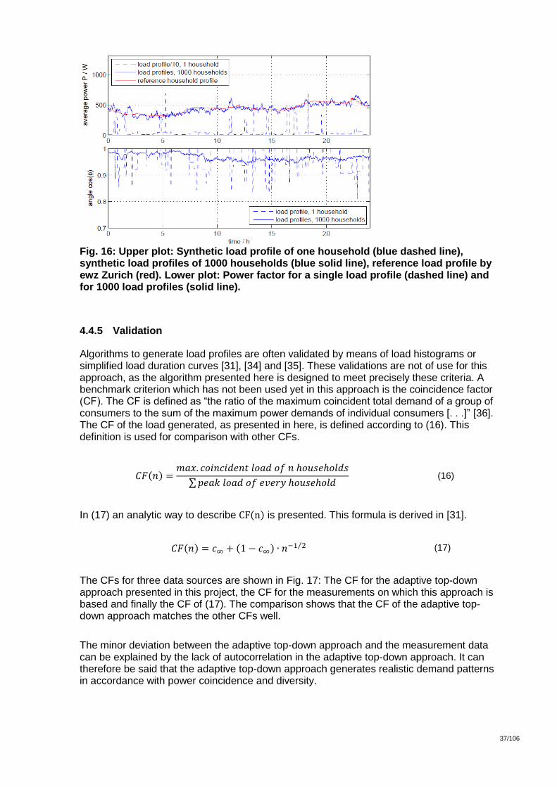
In Fig. 16 (top) a single load profile (blue dashed line) and the average power of 1000 load profiles (blue solid line) are shown. The red line shows the reference load profile. The corresponding power factor for both the single and the average load profiles is shown in the lower part of Fig. 16.

37/106


37

Fig. 16: Upper plot: Synthetic load profile of one household (blue dashed line), synthetic load profiles of 1000 households (blue solid line), reference load profile by ewz Zurich (red). Lower plot: Power factor for a single load profile (dashed line) and for 1000 load profiles (solid line).

4.4.5 Validation

Algorithms to generate load profiles are often validated by means of load histograms or simplified load duration curves [31], [34] and [35]. These validations are not of use for this approach, as the algorithm presented here is designed to meet precisely these criteria. A benchmark criterion which has not been used yet in this approach is the coincidence factor (CF). The CF is defined as “the ratio of the maximum coincident total demand of a group of consumers to the sum of the maximum power demands of individual consumers [. . .]” [36]. The CF of the load generated, as presented in here, is defined according to (16). This definition is used for comparison with other CFs.

( )

∑ (16)

In (17) an analytic way to describe ( ) is presented. This formula is derived in [31].

( ) ( ) ⁄ (17)

The CFs for three data sources are shown in Fig. 17: The CF for the adaptive top-down approach presented in this project, the CF for the measurements on which this approach is based and finally the CF of (17). The comparison shows that the CF of the adaptive top-down approach matches the other CFs well.

The minor deviation between the adaptive top-down approach and the measurement data can be explained by the lack of autocorrelation in the adaptive top-down approach. It can therefore be said that the adaptive top-down approach generates realistic demand patterns in accordance with power coincidence and diversity.

38/106


38

Fig. 17: Coincidence Factor (CF): Adaptive Top-Down Approach, measurement data and CF published in [31].

This validation is done using individual load profiles of one day, applying (16). If the validation is carried out with load profiles of one year instead, the CF would decrease even more to about 0.1 for 100 households. This is due to the fact that power peaks of a single household occur not every day, but with a high probability at least once a year. If on top of the yearly load profile a temporal resolution of one hour is applied (instead of one minute), Fig. 17 becomes true again. The high power peaks of single households are smoothed out (chapter 3).

4.4.6 Use of the Load Profile Generator in DiGASP

During the main project time, no high resolution measurement data was available. Household loads were therefore simulated using the load profile generator which was fed with artificial bottom-up load patterns. Receiving one year measurement data from ewz in autumn 2013, the main simulation results were repeated and validated with both real measurement data as well as artificial load profiles generated with the load profile generator using the new measurements as input data.

4.5 Meteo Data Generator

This chapter provides a short summary of the report "Development and Validation of the DiGASP Weather Generator" [5].

4.5.1 Introduction to the Irradiance Generator

The irradiance generator is at the heart of the weather generator and built up from the following steps: Using the Heliosat method hourly values of the clear sky index k, which is a measure for cloud transmittance, are calculated from nine years of Meteosat Second Generation measurements. The goodness of the distribution of these values is improved using a new method based on feature transformation. To be able to create more than nine synthetic years the diurnal patterns of neighbouring days are randomly interchanged. Using a modified version of the Skartveit and Olseth method, minute values of k are generated from the hourly values. Multiplication with the clear sky irradiance from the Dumortier model gives the high resolution global horizontal irradiance.

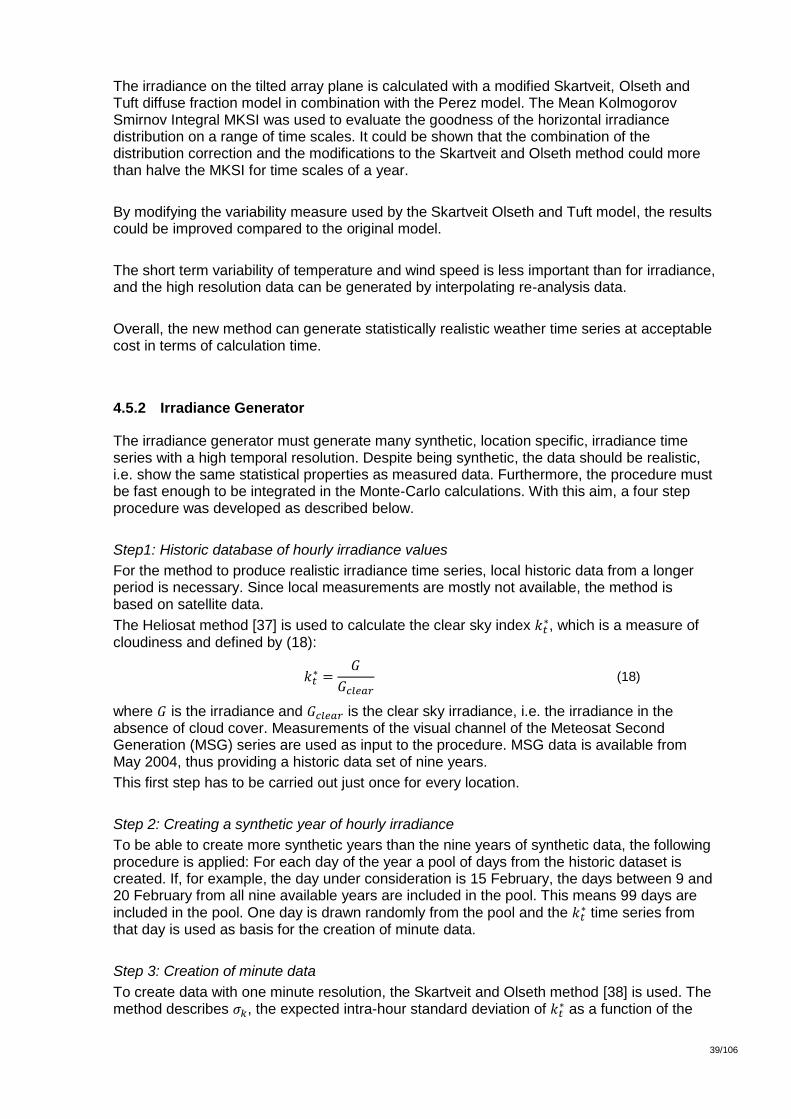
39/106


39

The irradiance on the tilted array plane is calculated with a modified Skartveit, Olseth and Tuft diffuse fraction model in combination with the Perez model. The Mean Kolmogorov Smirnov Integral MKSI was used to evaluate the goodness of the horizontal irradiance distribution on a range of time scales. It could be shown that the combination of the distribution correction and the modifications to the Skartveit and Olseth method could more than halve the MKSI for time scales of a year.

By modifying the variability measure used by the Skartveit Olseth and Tuft model, the results could be improved compared to the original model.

The short term variability of temperature and wind speed is less important than for irradiance, and the high resolution data can be generated by interpolating re-analysis data.

Overall, the new method can generate statistically realistic weather time series at acceptable cost in terms of calculation time.

4.5.2 Irradiance Generator

The irradiance generator must generate many synthetic, location specific, irradiance time series with a high temporal resolution. Despite being synthetic, the data should be realistic, i.e. show the same statistical properties as measured data. Furthermore, the procedure must be fast enough to be integrated in the Monte-Carlo calculations. With this aim, a four step procedure was developed as described below.

Step1: Historic database of hourly irradiance values

For the method to produce realistic irradiance time series, local historic data from a longer period is necessary. Since local measurements are mostly not available, the method is based on satellite data.

The Heliosat method [37] is used to calculate the clear sky index , which is a measure of

cloudiness and defined by (18):

(18)

where is the irradiance and is the clear sky irradiance, i.e. the irradiance in the absence of cloud cover. Measurements of the visual channel of the Meteosat Second Generation (MSG) series are used as input to the procedure. MSG data is available from May 2004, thus providing a historic data set of nine years.

This first step has to be carried out just once for every location.

Step 2: Creating a synthetic year of hourly irradiance

To be able to create more synthetic years than the nine years of synthetic data, the following procedure is applied: For each day of the year a pool of days from the historic dataset is created. If, for example, the day under consideration is 15 February, the days between 9 and 20 February from all nine available years are included in the pool. This means 99 days are included in the pool. One day is drawn randomly from the pool and the

time series from that day is used as basis for the creation of minute data.

Step 3: Creation of minute data

To create data with one minute resolution, the Skartveit and Olseth method [38] is used. The method describes , the expected intra-hour standard deviation of

as a function of the

40/106


40

standard deviation of three hourly values. For each hour a value of is randomly drawn from a Weibull distribution whose shape is determined by . The value of is in its turn used to determine the parameters of a linear combination of two β-functions, that describe the distribution of the variable , which is a normalised

. The value of is drawn randomly

from this distribution to obtain high resolution versions of , which is finally multiplied with

to obtain the high resolution values of , where is calculated with the Dumortier model [39].

Fig. 18 shows the synthetic data for a sample day in comparison with the original measured data. The distribution of the synthetic data is compared with the distribution of measured data in Fig. 19. It shows that, although the Skartveit and Olseth method was originally designed to produce data with a five minute resolution, there is a relatively good agreement between the two distributions. A further adaptation of the method is in development.

Fig. 18: Example of a measured and synthetic irradiance time series.

Fig. 19: Distribution of measured and synthetic irradiance with a one-minute resolution based on two years of measurements at Oldenburg University.

41/106


41

4.5.3 Generator for Wind- and Temperature Data

For the temperature and wind data, measurements from the Affoltern weather station provided by MeteoSwiss are used. The data has a temporal resolution of ten minutes. Since temperature and wind speed do not fluctuate as rapidly as solar irradiance, a cubic spline interpolation method is used to obtain a one-minute resolution. To conserve the correlation with the irradiance data, data from the same dates that were drawn in the irradiance lottery are used. If the temperature or wind data was not available for that date, it was taken from the same day in a different year. The year was determined by comparing the irradiance sums of the chosen date.

4.6 Monte Carlo Simulation

Monte Carlo simulations are often used to numerically compute or estimate values, which could not be calculated arithmetically or only with considerable effort. Three major steps are necessary:

1. Randomisation of input data

2. Calculation of output

3. Evaluation of output (e.g. calculation of mean value from output)

In this project Monte Carlo simulations are used to calculate the distribution of maximum voltages in a distribution grid.

4.6.1 Problem Formulation

Many simulations which are performed in this project are based on the analysis of worst case situations. The PV hosting capacity for example is derived by simulating one full year with various PV penetration scenarios. The PV penetration is increased unless the voltage rises above a critical value, usually given by . The corresponding PV penetration is defined as the PV hosting capacity of the grid.

The aim of the Monte Carlo simulations is to investigate and visualise the distribution of these worst case situations. If a certain overvoltage is likely to occur once in a year, but very unlikely to occur repeatedly, there might be better solutions to handle this overvoltage than to dimension the grid for it.

4.6.2 Required Number of Simulations

In the corollary 1 of [40], Calafiore states the minimum number of scenarios which is required to satisfy a confidence level and a probability level of a -dimensional problem (19).

⌈

(

)

(

)⌉ (19)

42/106


42

To calculate the expectation value ( ) of the maximum voltage on a given summer day with a confidence level of ( ), only 26 scenarios are required. If the 90-percentile

is to be calculated ( ), 155 scenarios are needed. For the 98-percentile, this figure is 924 and for the 99-percentile it is 1983.

In this project, the number of scenarios used is 1000. The results presented in Fig. 65 have therefore a confidence level of up to the 98-percentile.

4.6.3 Limitations

The major drawback of Monte Carlo simulations is the req7uired computational power. To simulate a full year with a temporal resolution of one minute, 525'600 time steps must be simulated. If 1000 scenarios must be simulated in a Monte Carlo simulation, the simulation consists of almost 525.6 million time steps and thus 525.6 million power flow problems which must be solved. Even if a fast computer could solve 1000 power flow problems within a second, it would need more than six days and nights to perform the simulation.

This is neither practical nor necessary. With the following two measures, this problem is mitigated massively:

A broad range of scenarios and methods are simulated in this project. However, Monte Carlo simulations must mainly investigate the statistical nature of solar irradiance vs. domestic load profiles. Therefore, only a much reduced number of scenarios and methods are actually simulated with a Monte Carlo approach (chapter 0).

Searching for the maximum PV hosting capacity of a distribution grid, only the critical time steps must be simulated. These are mainly weekends in summer (low load, high PV production). The critical voltages are found using the voltage sensitivity matrix (section 4.2.1).

43/106


43

5 Control Algorithms

"Replace copper with intelligence" could be the slogan of this project. In this chapter the "intelligent alternatives to copper" are presented: They relate to the seven methods and control algorithms which allow the PV hosting capacity of an LVDG to be increased.

All control algorithms used in this project were presented in various publications written by various authors. It is an objective of this project to collect and adapt these algorithms to the simulation framework, to optimise them if necessary and, most importantly, to compare their performance in terms of increasing PV hosting capacity of an LVDG. Whenever the control algorithms are modified, the modifications are explained in detail.

The following eight sections (section 5.1 to section 5.8) contain eight methods which can be used to integrate PV into the LVDG. The first method, called "DACHCZ", is currently used in Switzerland to determine the PV hosting capacity of an LVDG [41]. In the following studies, it is always used as the reference method if the performance of another method is shown with relative figures.

5.1 DACHCZ

The "Technical Rules for the Assessment of Network Disturbances (DACHCZ)" published by the associations of electric utilities of Germany, Austria, Switzerland and the Czech Republic accept in normal situations a maximum relative voltage rise of 3 % in the low voltage grid (reference). To compute the voltage rise, all loads must be set to zero, and the maximum possible power output of all PV power systems must be considered with a coincidence factor of one. This is the most important rule in Switzerland, according to which PV power systems are to be installed today.

Not only in the DACHCZ approach, but in all further computations in this project, a maximum voltage rise of 3 % is considered to be the limit of the voltage tolerance. The computation of this 3 % is however done with a range of different assumptions.

5.2 Correlation with Load

In this power flow computation method, the loads in the grid are no longer set to zero. Realistic load patterns are used to compute the load power which reduces and limits the PV production peak at any time. In order to obtain realistic load patterns with a high temporal resolution, the load profile generator is presented in section 4.4.

5.3 Reactive Power Control (RPC)

In accordance with Swiss grid codes, PV power plants must supply their power with a power factor of cos(phi) = 1. In Germany, this rule was changed in 2011 in accordance with the VDE AR 4105 [42], where a dynamic power factor down to 0.95 lagging is required in normal cases. Consuming reactive power while feeding in active power will reduce the voltage rise in a power system and therefore lead to higher PV hosting capacity of the grid.

44/106


44

RPC is often done using a droop factor [43]. If the grid voltage exceeds the voltage

, the PV inverter starts to consume reactive power (under-excited or inductive

operation). The droop factor is defined as shown in (20).

(20)

where is the maximum reactive power capacity of the inverter and the

voltage, at which the inverter will consume . The reactive power consumption is

given by (21).

( ) (21)

is bound by three constraints, (22) to (24):

(22)

(23)

( ) ( ) (24)

where is the active power output, is the apparent power output, is the rated AC

power, ( ) is the power factor and ( ) is the minimum power factor of the PV

plant at node .

5.4 Active Power Curtailment (APC)

Curtailing PV power or, expressed alternatively cutting the peak power will cause energy losses. Because the power peaks of PV power occur relatively seldom, only little energy is lost even when a substantial percentage of the power is cut. Using APC is therefore a powerful instrument to integrate more PV energy in the power grid.

5.4.1 Constant APC

If a PV power plant is designed with an APC ratio < 1, APC is applied intrinsically. This is the most simple and widespread use of APC and therefore mainly used in the simulations of this project.

5.4.2 Smart APC

The purpose of APC is to relieve the grid. The same effect as curtailing active power can be reached if an additional load is connected to the grid at the same place where the PV power

45/106


45

plant is located. The power of the load can now be withdrawn from the PV power in order to calculate their effect on the grid. In practice this means that not the output of the PV power plant must be limited, but the maximum power flow from a building to a grid.

5.4.3 Droop-based APC

The APC algorithm works in a similar manner to that described in Tonkoski et al. [44]. The PV power inverter connected to node of the grid measures the local AC grid voltage .

If this voltages exceeds the individually configured voltage , the power output of the

inverter is reduced using a constant droop factor , see (25).

(25)

where is the rated power of the PV plant at node and the maximum

tolerable voltage. The power output of the PV plant is then calculated using (26).

( ) (26)

In a very simple grid (one feeder, one line, one load (section 6.1), the droop-based APC is identical to the smart APC (5.4.2).

5.4.4 Stability Issues with Droop-based APC

If RPC or APC are used as a function of the grid voltage, this corresponds to a closed-loop control system which can potentially be instable. A stabiliser is proposed in [6]. Whenever droop based APC algorithms are used in DiGASP, this stabiliser is used. Using this stabiliser for multi node networks, its performance is however far from perfect: In a 10 node radial network for example, roughly 10 to 20 iteration steps were needed for the algorithm to converge. This is the reason, why many simulations in this project are made using a static and not a droop based APC (constant limitation of the active power).

5.4.5 Optimised APC

An approach to optimise the constant APC is derived in Appendix A.

5.5 Different Orientations of PV Systems

The daily peak of the irradiance occurs at midday, if a PV power plant is installed horizontally or elevated southwards. If PV panels are mounted eastwards or westwards, the peak is shifted into the morning or afternoon. As it is the peak power which mainly limits the hosting capacity, shifting the peak can increase it.

46/106


46

5.6 Storage

Instead of curtailing peak power to relieve the power grid, excess energy can be stored in decentralised storage systems. From the power and energy rating of the storage, an additional PV hosting capacity can be determined.

5.7 Demand Side Management (DSM)

Whether or not DSM contributes significantly to the PV hosting capacity of a power grid depends largely on the assumptions which are considered. In this project, it is simply assumed that water boilers are available in every household, and that they can be charged whenever required within 24 hours.

5.8 On Load Tap Change Transformer (OLTC)

The distribution system is normally run asymmetrically: The secondary transformer voltage (LV) is set to about 1.03 pu, which leads to a high negative voltage tolerance, but only to a small positive voltage tolerance. Having an OLTC transformer, the tap change ratio and thus the secondary voltage can be shifted while the transformer is in operation. With this, the positive voltage tolerance can roughly be doubled.

47/106


47

6 Simulation Results and Interpretation

Eight different methods and algorithms to compute the PV hosting capacity of an LVDG have been described in chapter 5. In this chapter the results of the simulations performed with these methods are presented. Basically all methods are applied to the following three different networks:

1. Lumped model: The most simple network consisting of one feeder and one node.

2. Radial network: A single feeder consisting of an arbitrary number of nodes (normally ten).

3. Case Study: The network "Luchswiesenstrasse" of ewz in Zurich, a feeder consisting of two parallel 1000 kVA transformers and roughly 160 nodes.

The influence of various parameters such as number of households in a grid or line length in a radial network on the PV hosting capacity is of major interest. Therefore the results are presented in graphs using several variable parameters. If a certain parameter is relevant but not varied, the standard values given in Tab. 1 are used in the simulation. Deviations from these standard parameters are described separately, if applicable.

Parameter Shortcut Range Standard value

number of households nrHH 1 – 1000 -

Number of nodes 1 – 20 10

tilt angle 0° – 90° 0° / 20°

module orientation N/E/S/W/EW S

line length 100 m – 2000 m 100 m per segment

power factor cos(phi) 0.8 – 1.0 1.0

APC ratio 0.5 – 1.0 1.0

correlation with loads corr yes / no no

Tap change ratio TCR 0.97 – 1.03 1.0

Location Zürich / Jungfraujoch Zürich

Tab. 1: List of parameters, their range and standard values used in the simulations.

6.1 Lumped Model

The "lumped model" consists of the simplest possible network: One feeder, one line and one node (Fig. 20). At the node, a load and a PV power plant is connected. The load consists of 1 to 1000 households, the PV power plant is maximised in accordance with the following rules:

48/106


48

Maximum voltage dip: 6 % --> defines the grid impedance with given loads

Maximum voltage rise: 3 % --> defines the maximum PV hosting capacity

With the lumped model, a number of effects that appear when PV and household loads are connected to the same grid can be studied. One important example is the effect of correlation between PV and load. This principle can be studied even if no specific grid (or only the "lumped model grid" in Fig. 20) is considered.

The results presented in this and the following chapters will show that not only the benefit of correlation with loads, but even the effects of most of the other methods to compute the PV hosting capacity of an LVDG can be predicted, if the results of the lumped model simulation are known.

Fig. 20: Simple network consisting of one feeder, one line and one node (lumped model).

The line in Fig. 20 is dimensioned for a voltage dip of 6 % at peak load. The line impedance depends therefore mainly on the number of households which are connected to the line. In other words: The weakest possible line to serve the households safely is chosen. This is of course a rather conservative approach – in reality many lines are overdimensioned. The generic results of DiGASP apply therefore mainly for those grids which are operated at their limits only to serve the household loads.

6.1.1 DACHCZ

The amount of PV in the grid (the PV penetration) is increased in this calculation until the maximum relative voltage rise (all loads are set to zero in this simulation) reaches 3 %. The maximum PV power per household ranges from 4.8 kWp per household (one household connected to the node) to 0.4 kWp per household (1000 households). This corresponds to a PV penetration of over 150 % for the one household case and about 15 % for the 1000 household case (Fig. 21). The reason for this large decrease is the coincidence factor of the household loads, which allows reducing the grid (diameter of cables) per household in the 1000 household case. Fig. 21 is therefore quite in line with the plotted values of the coincidence factor (Fig. 17) provided that load profiles of one whole year are considered. In other words: The power peaks of a single household lead to a massive overdimensioning in the one household case. PV power plants profit from this oversized grid.

Fee

de

r

Line

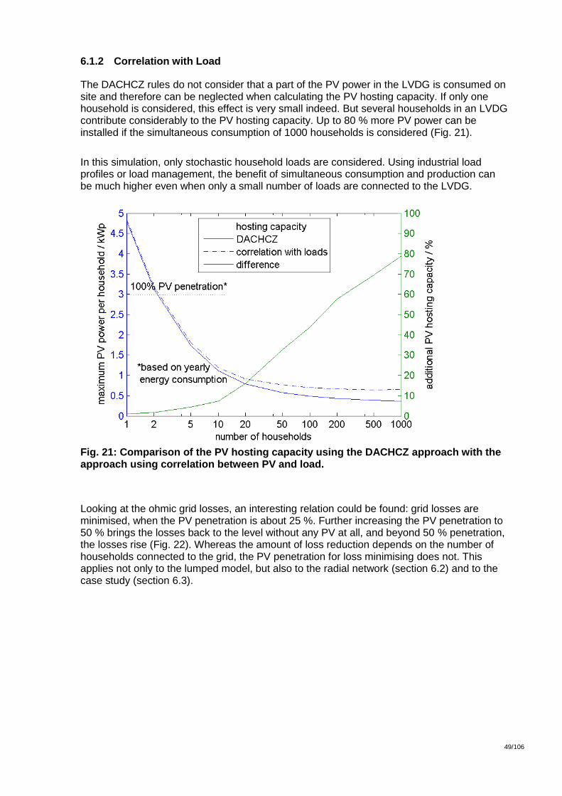
49/106


49

6.1.2 Correlation with Load

The DACHCZ rules do not consider that a part of the PV power in the LVDG is consumed on site and therefore can be neglected when calculating the PV hosting capacity. If only one household is considered, this effect is very small indeed. But several households in an LVDG contribute considerably to the PV hosting capacity. Up to 80 % more PV power can be installed if the simultaneous consumption of 1000 households is considered (Fig. 21).

In this simulation, only stochastic household loads are considered. Using industrial load profiles or load management, the benefit of simultaneous consumption and production can be much higher even when only a small number of loads are connected to the LVDG.

Fig. 21: Comparison of the PV hosting capacity using the DACHCZ approach with the approach using correlation between PV and load.

Looking at the ohmic grid losses, an interesting relation could be found: grid losses are minimised, when the PV penetration is about 25 %. Further increasing the PV penetration to 50 % brings the losses back to the level without any PV at all, and beyond 50 % penetration, the losses rise (Fig. 22). Whereas the amount of loss reduction depends on the number of households connected to the grid, the PV penetration for loss minimising does not. This applies not only to the lumped model, but also to the radial network (section 6.2) and to the case study (section 6.3).

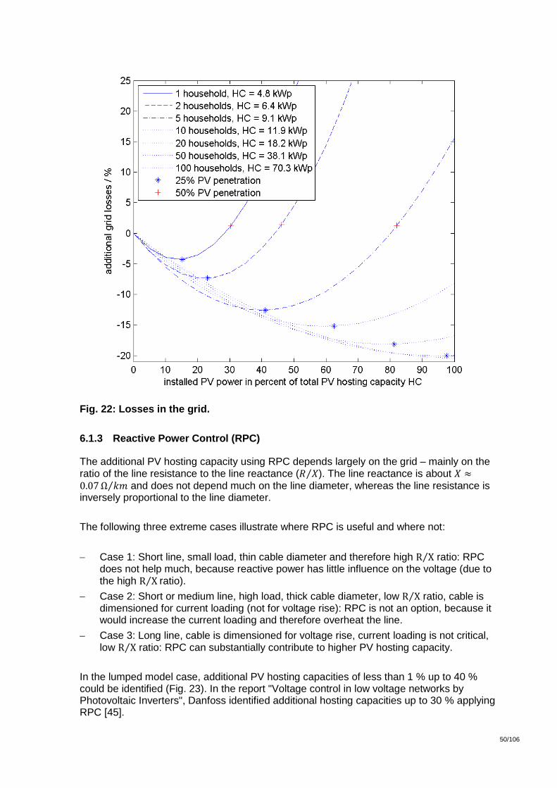
50/106


50

Fig. 22: Losses in the grid.

6.1.3 Reactive Power Control (RPC)

The additional PV hosting capacity using RPC depends largely on the grid – mainly on the ratio of the line resistance to the line reactance ( ⁄ ). The line reactance is about ⁄ and does not depend much on the line diameter, whereas the line resistance is inversely proportional to the line diameter.

The following three extreme cases illustrate where RPC is useful and where not:

Case 1: Short line, small load, thin cable diameter and therefore high ⁄ ratio: RPC does not help much, because reactive power has little influence on the voltage (due to the high ⁄ ratio).

Case 2: Short or medium line, high load, thick cable diameter, low ⁄ ratio, cable is dimensioned for current loading (not for voltage rise): RPC is not an option, because it would increase the current loading and therefore overheat the line.

Case 3: Long line, cable is dimensioned for voltage rise, current loading is not critical, low ⁄ ratio: RPC can substantially contribute to higher PV hosting capacity.

In the lumped model case, additional PV hosting capacities of less than 1 % up to 40 % could be identified (Fig. 23). In the report "Voltage control in low voltage networks by Photovoltaic Inverters", Danfoss identified additional hosting capacities up to 30 % applying RPC [45].

51/106


51

Fig. 23: Reactive power control depending on line length.

6.1.4 Active Power Curtailment (APC)

If a PV power plant is equipped with a inverter (instead of a inverter), the PV power in the grid can roughly be doubled. The PV energy in the grid is not doubled, because a part of it is curtailed. Fig. 24 illustrates the energy which is lost (red part) and fed

into the grid (black part). The lost energy is only about of the total energy.

52/106


52

Fig. 24: Curtailing of PV power.

The amount of energy which is actually lost by the application of APC is highly dependent on the yearly sum of irradiation into the plane of modules. Fig. 25 shows the relation between the APC ratio and the yearly energy curtailment for the locations Zürich and Jungfraujoch (in the Alps, 3'471 m above sea level), for four and five different tilt angles.

An inverters power rating in Zürich should hence not be much bigger than of the nominal DC power. If the PV modules are not inclined towards the south but installed

horizontally, even with APC ratio less than one per cent of the energy yield is lost.

A completely different situation is predominant on Jungfraujoch. Due to much higher solar

irradiation as well as high albedo caused by the snow, even an APC ratio of leads to an energy loss of .

Fig. 25: Yearly energy curtailment as a function of the APC ratio.

53/106


53

Plotting the additional PV hosting capacity versus the loss of energy yield, Fig. 26 is obtained. This graph is plotted for the location of Zurich, but it looks similar to the graph for Jungfraujoch. Furthermore it does not depend so much on the tilt angle of the PV modules. The reason is that power peaks at a sunny place with optimally tilted PV modules are much higher than power peaks of the same plant at a less sunny place. Curtailing a certain percentage of energy will therefore lead to different APC ratios, but to similar (relative) increases of the PV hosting capacity.

Fig. 26: Additional PV hosting capacity using APC.

Using "smart APC", the energy consumed by the household loads simultaneously with the PV power production must not be curtailed by the power inverter, but can be recovered. If only one household is connected to a PV power plant, roughly of the energy loss can

be recovered (for an APC ratio of ). However, if the smart APC approach is used for 100 households and the corresponding maximum PV penetration, almost of the potential energy curtailment can be recovered.

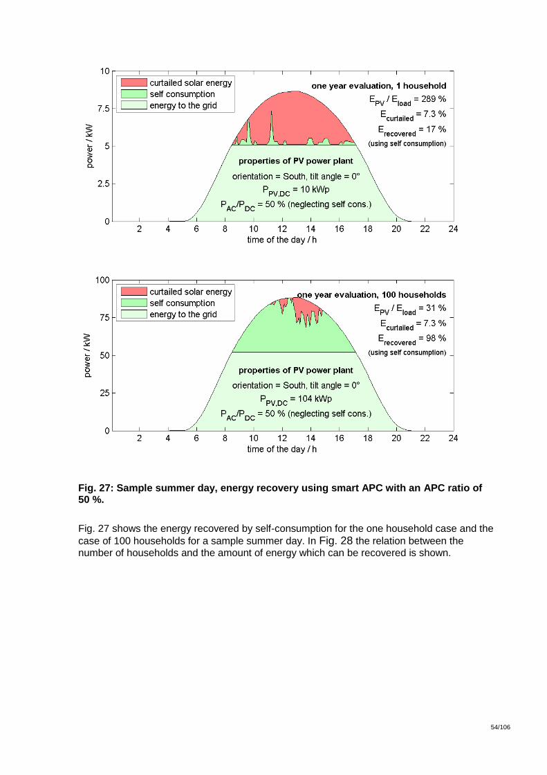
54/106


54

Fig. 27: Sample summer day, energy recovery using smart APC with an APC ratio of 50 %.

Fig. 27 shows the energy recovered by self-consumption for the one household case and the

case of 100 households for a sample summer day. In Fig. 28 the relation between the

number of households and the amount of energy which can be recovered is shown.

55/106


55

Fig. 28: Energy recovery using smart APC with an APC ratio of 50 %.

Fig. 25 to Fig. 28 promote low APC ratios, but sizing of the inverter is not only a question of

optimising APC losses. If RPC is used, the inverter needs apparent power reserves. If an excessively small inverter is used, there are no reserves left. Having an inverter which operates a substantial part of its time at nominal power, the lifetime of the inverter might be reduced.

The idea of operating a power inverter most of the time in its highest efficiency point is however not as important as 20 years ago, because the efficiency curves of inverters are fairly constant over a broad range of operating points.

6.1.5 Different Orientations of PV Systems

For most of the previous simulations, PV modules were oriented towards the South. If the PV modules are not oriented towards the South, but for example towards East and West, the PV hosting capacity changes (Fig. 29).

There are two effects which affect the change of the PV hosting capacity: Different azimuth- and tilt angles result both in different energy yields and different power peaks.

56/106


56

Fig. 29: Variable orientation and tilt angle change the energy per maximum AC power and thus the PV hosting capacity.

The red line in Fig. 29 represents the modules oriented to the South. This is not a bad option, as the ratio between energy yield and power peak (and thus the PV hosting capacity) is high. If the PV modules are turned towards the East or West, the energy yield decreases faster than the power peak and the PV hosting capacity therefore decreases also. For example the peak power of a PV power plant which is located in Zürich and oriented towards the East with a tilt angle of 70 degrees is still as high as the peak of a horizontally mounted PV power

plant. The energy yield in contrast decreases from almost ⁄ to ca. ⁄ . If only such plants were installed in a grid, the PV hosting capacity would

thus decrease by about .

It is however the mixture of different orientations which increases the PV hosting capacity: Having an East-West-oriented PV plant, the PV hosting capacity of the LVDG increases by roughly , if the tilt angle is about . For standard tilt angles of , the PV hosting capacity does not change much compared with a horizontal installation.

57/106


57

In Fig. 30 the combination of APC, correlation between PV and load and different orientations and tilt angles are investigated. The question to be answered by Fig. 30 is: "What percentage of the available solar energy can be fed into the grid, if smart APC is used, and the PV modules are oriented towards the East and West with variable tilt angles?" First of all, the graphs give the known picture if the tilt angle of the PV modules is zero. Less than

of the solar energy is fed into the grid in the one household case, and close to if more than 100 households are connected at the same node. If the tilt angle is now increased

to about , all energy can be fed into the grid independently of the number of households.

A combination of different orientations and smart APC therefore enables a doubling of the PV hosting capacity of an LVDG without wasting any solar energy.

The effect of the combination of APC and different orientations of the module (East, South and East-West) can be found in Appendix B: Combination of Smart APC and Different Module Orientations and Tilt Angles.

The self consumption ratio (amount of PV power consumed real-time on site) is presented in Appendix C: Self Consumption Ratio, the self sufficiency ratio (amount of energy consumed delivered by PV real-time on site) is shown in Appendix

58/106


58

D: Self Sufficiency Ratio for Different Module Orientations. Both ratios state the relative benefit of East-West oriented modules, but in both cases this benefit is only a few per cent additional self consumption and self sufficiency. Surprisingly, the North façade is most beneficial for the grid. But as the energy yield of a North façade system is about four times smaller than the yield of a corresponding optimal tilted system, this benefit is not in reality a determining factor.

Fig. 30: Combination of APC, correlation with load and different orientations.

6.1.6 Storage

The basic principle of the use of storage is illustrated in Fig. 31. The AC output of a PV power plant combined with a storage system is limited to . The energy which is

provided in excess of is stored locally and released when the power output of the PV power plant drops under .

59/106


59

Fig. 31: Principal use of storage in the LVDG.

The PV hosting capacity in this case is doubled; orientation of the PV modules, correlation between generation and load etc. is ignored.

The main variable of interest in this simulation is the capacity of the storage. In Fig. 32 the additional PV hosting capacity is given as a function of the storage capacity in nominal hours of operation of the PV power plant. The four graphs (each representing one PV module orientation) each consist of four segments. Starting from bottom left, each segment stands for a typical storage use.

Segment 1 (from 0 to about 0.1 nominal operating hours): In this segment, the very peaks of the power production are stored. As the APC analysis already showed (section 6.1.4), there is not much energy in the power peaks. Therefore a large increase of the PV hosting capacity can be reached with only a very limited storage capacity. It might however be cheaper to simply curtail this energy than to install storage capability.

Segment 2 (from 0.1 to 4 nominal operating hours): In the second segment, the storage is charged over one day at the most and discharged by night. Four nominal operating hours is precisely the amount of storage that is needed to run a PV power plant for two consecutive sunny summer days with a constant power output over 24 hours.

Segment 3 (from 4 to 8 nominal operating hours): If the energy of more than four nominal operating hours is stored, energy must be stored over at least two days. A large amount of storage is therefore needed, with a rather small increase in the PV hosting capacity.

Segment 4 (more than 8 nominal operating hours): The trend continues – increasing the storage capacity only marginally increases the PV hosting capacity. Storing energy over several days or even from summer to winter needs very large amounts of storage, but the PV hosting capacity remains almost constant.

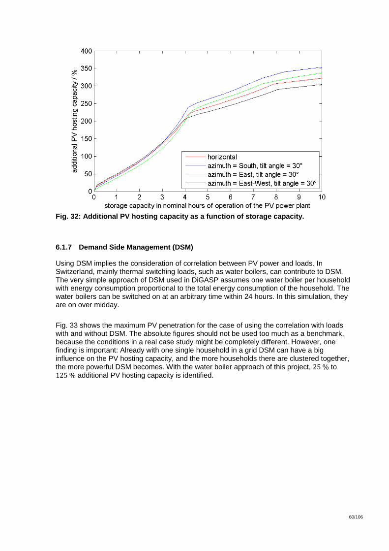
60/106


60

Fig. 32: Additional PV hosting capacity as a function of storage capacity.

6.1.7 Demand Side Management (DSM)

Using DSM implies the consideration of correlation between PV power and loads. In Switzerland, mainly thermal switching loads, such as water boilers, can contribute to DSM. The very simple approach of DSM used in DiGASP assumes one water boiler per household with energy consumption proportional to the total energy consumption of the household. The water boilers can be switched on at an arbitrary time within 24 hours. In this simulation, they are on over midday.

Fig. 33 shows the maximum PV penetration for the case of using the correlation with loads with and without DSM. The absolute figures should not be used too much as a benchmark, because the conditions in a real case study might be completely different. However, one finding is important: Already with one single household in a grid DSM can have a big influence on the PV hosting capacity, and the more households there are clustered together, the more powerful DSM becomes. With the water boiler approach of this project, to additional PV hosting capacity is identified.

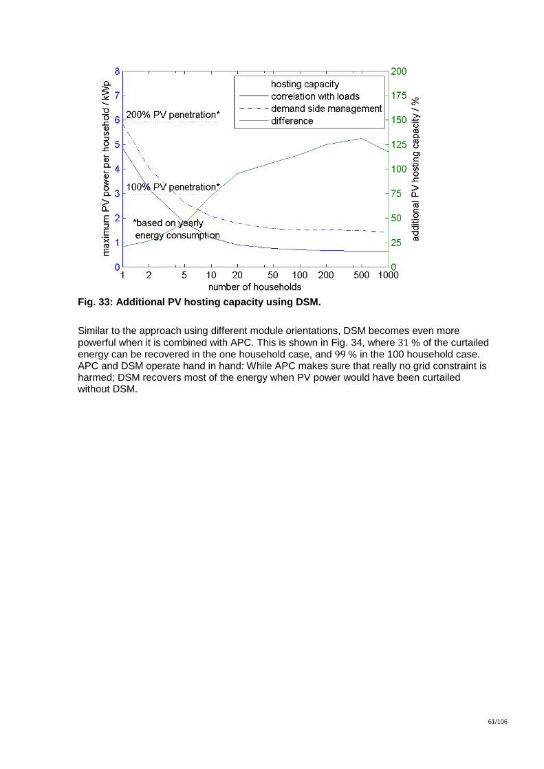
61/106


61

Fig. 33: Additional PV hosting capacity using DSM.

Similar to the approach using different module orientations, DSM becomes even more

powerful when it is combined with APC. This is shown in Fig. 34, where of the curtailed energy can be recovered in the one household case, and in the 100 household case. APC and DSM operate hand in hand: While APC makes sure that really no grid constraint is harmed; DSM recovers most of the energy when PV power would have been curtailed without DSM.

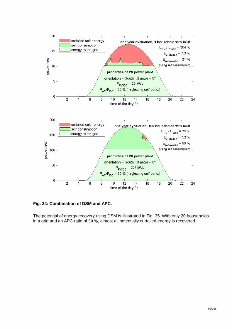
62/106


62

Fig. 34: Combination of DSM and APC.

The potential of energy recovery using DSM is illustrated in Fig. 35. With only 20 households in a grid and an APC ratio of , almost all potentially curtailed energy is recovered.

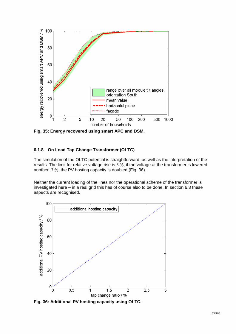
63/106


63

Fig. 35: Energy recovered using smart APC and DSM.

6.1.8 On Load Tap Change Transformer (OLTC)

The simulation of the OLTC potential is straightforward, as well as the interpretation of the results. The limit for relative voltage rise is , if the voltage at the transformer is lowered

another , the PV hosting capacity is doubled (Fig. 36).

Neither the current loading of the lines nor the operational scheme of the transformer is investigated here – in a real grid this has of course also to be done. In section 6.3 these aspects are recognised.

Fig. 36: Additional PV hosting capacity using OLTC.

64/106


64

6.2 Radial Network

A radial network consisting of one feeder and ten nodes is used as a generic simulation approach. Each node is equipped with between one and twenty households and a PV power plant.

Fig. 37: Generic network consisting of one feeder and ten nodes.

The dimensioning of the line is done in a similar manner as for the lumped model: The weakest possible line to serve the loads is chosen. To keep the simulation as generic as possible, the line from the feeder to the last node always has the same diameter. The diameter depends again on the peak load and therefore on the number of households connected to each node.

As noted previously (section 6.1), many simulation results using the radial network are almost identical to those using a lumped model. In the following sections the simulation results are presented. The focus is therefore on characterising similarities and differences to the lumped model simulations.

6.2.1 DACHCZ

The DACHCZ approach is a typical example where the results of the lumped load model (Fig. 21) and the radial network (Fig. 38) are very similar. Because the radial network has ten nodes, the minimum number of households investigated here is ten. The maximum number of households is limited to 200 (which means 20 households per node), otherwise the power supply with only one line would no longer be realistic.

One fact is rather surprising in this simulation: Basically the PV hosting capacity falls as more households are connected to the grid. This effect was explained previously (section 6.1). However, if more than 100 households are connected, the PV hosting capacity rises again. This is due to the fact that the power factor ( ) of the load is slightly inductive and the line

for 200 households (which has a low ⁄ ratio) must therefore be selected to be thicker than normal. As the PV power plants operate with ( ) , the ratio PV to load can be increased.


Having the weakest possible grid to serve the loads, the PV hosting capacity of a lumped model represents the previously mentioned 10 node feeder quite well in several aspects.

1 2 9 10

Fee

de

r

Line

Node

65/106


65

One of them is the additional PV hosting capacity respecting the correlation between PV and load (Fig. 38).

Fig. 38: Comparison of the PV hosting capacity using the DACHCZ approach with the approach using correlation between PV and load.

A familiar picture can be shown not only in terms of PV hosting capacity, but also regarding the grid losses: Fig. 39 confirms the findings of Fig. 22. The losses are minimised at a PV penetration of roughly , independent of the number of households and thus the grid impedance. The amount of loss reductions however depend on the number of households and range from for only a few households to for several hundred households.

Just to forestall one result of the case study: In the real grid (section 6.3), the grid losses are also minimised at PV penetration, saving about of the loss energy. A very similar result was presented by Danfoss [47] in summer 2013. Without being able to adduce evidence, the minimisation of the grid losses at PV penetration seems to be a general rule.

66/106


66

Fig. 39: Grid losses depending on the PV penetration and the number of households.


Using RPC is a good option if the voltage rise on a line is critical, but not the thermal loading. In this case the additional PV hosting capacity found in Fig. 40 is found for the test feeder.

Fig. 40: PV hosting capacity and additional hosting capacity using RPC.

RPC is mainly a question of the ratio or the grid impedance angle. With a ratio

larger than about five (this corresponds to a grid impedance angle of , the effect of RPC is

rather small (Fig. 41). Ignoring the transformer, a line diameter larger than is

67/106


67

necessary to get ⁄ . Similar results are obtained by Shayani et al. [46], promising installed PV power of up to twice the load peak power when RPC is used.

Fig. 41: PV hosting capacity and additional hosting capacity using RPC depending on line length.


Again the prediction of the lumped model applies almost one to one to the ten node test

feeder. Fig. 42 shows the gain of additional PV hosting capacity, if an APC ratio of is applied. The percentage gain is independent of the number of households, because limiting the output power of a PV power plant to allows the installation of twice as much PV power independent of loads in the grid. The energy yield is not doubled but increases only with about - the reason is given in Fig. 26.

68/106


68

Fig. 42: PV hosting capacity and additional hosting capacity using APC.


The calculations shown in in Fig. 29 are repeated in Fig. 43 using only irradiance data from Zurich. The results are similar to those for the lumped model: The East-West system has the most beneficial energy to power ratio and therefore the maximum PV hosting capacity, but only for large tilt angles. For small tilt angles it is still the South oriented system which is ideal, because of its high energy yield which does not increase the maximum specific AC power output.

69/106


69

Fig. 43: Specific energy yield, maximum specific AC power and additional PV hosting capacity using different orientations.

70/106


70

6.2.6 Storage

Storage systems are not investigated for the single feeder model. The generic results in the lumped model section 6.1 apply even here – as long as no specific storage control adapted to the network topology is used. Such specific studies are however not within the scope of this project but can be found for example in [48], [49] and [50].


To present generic results for DSM is not possible as the potential of DSM is discussed somewhat controversially [51], [52] and [53]. Using the water boiler approach (see chapter 5.7) additional PV hosting capacity of to is found (Fig. 44). The differences to section 6.1.7 can be explained mainly with different load and water boilers which are used, however they have the same stochastic properties.

Fig. 44: Additional PV hosting capacity using DSM.


As mentioned in section 6.1.8, a tap change ratio of allows the doubling of the PV hosting capacity regarding voltage change (Fig. 45).

Similarly to the use of RPC, it is no longer sufficient to investigate only the voltage change, because thermal loading of the cables might now also become critical. In the simulation of

Fig. 45 there is however still a current loading reserve of about .

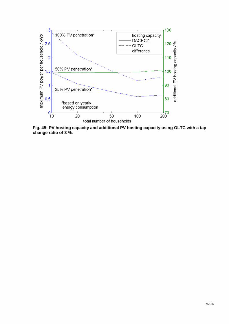
71/106


71

Fig. 45: PV hosting capacity and additional PV hosting capacity using OLTC with a tap change ratio of 3 %.

72/106


72

6.3 Case Study "Luchswiesenstrasse"

Both the lumped model and the radial feeder give generic results which can be used to predict the impact of PV systems on various LVDGs. But as they are generic, they do not represent a real system.

In this chapter, the part "Luchswiesenstrasse" of the Zurich LVDG is simulated using the methods demonstrated in the previous chapters. The most important parameters in the study are shown in Tab. 2. An overview of the area using Google Earth is given in Fig. 46.

Parameter Value

Number of facilities (households, companies etc.) 1550

Maximum load 1300 kW

Yearly consumption 5200 MWh

MV / LV transformer 2 x 1000 kVA

Number of lines / number of nodes 162 / 155

PV roof potential3 3624 kWp

Tab. 2: Parameters of the case study "Luchswiesenstrasse".

Fig. 46: Area "Luchswiesenstrasse" in Zurich.

3 All roofs used. PV module efficiency of 15 % assumed. The official solar cadastre of Zurich only

counts the roofs facing south, which results in a roughly 50 % lower PV roof potential.

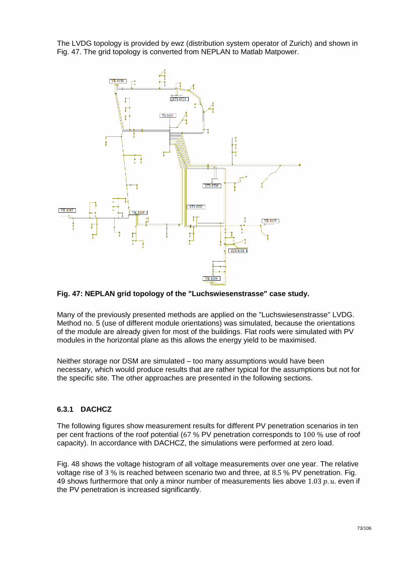
73/106


73

The LVDG topology is provided by ewz (distribution system operator of Zurich) and shown in Fig. 47. The grid topology is converted from NEPLAN to Matlab Matpower.

Fig. 47: NEPLAN grid topology of the "Luchswiesenstrasse" case study.

Many of the previously presented methods are applied on the "Luchswiesenstrasse" LVDG. Method no. 5 (use of different module orientations) was simulated, because the orientations of the module are already given for most of the buildings. Flat roofs were simulated with PV modules in the horizontal plane as this allows the energy yield to be maximised.

Neither storage nor DSM are simulated – too many assumptions would have been necessary, which would produce results that are rather typical for the assumptions but not for the specific site. The other approaches are presented in the following sections.

6.3.1 DACHCZ

The following figures show measurement results for different PV penetration scenarios in ten

per cent fractions of the roof potential ( PV penetration corresponds to use of roof capacity). In accordance with DACHCZ, the simulations were performed at zero load.

Fig. 48 shows the voltage histogram of all voltage measurements over one year. The relative

voltage rise of is reached between scenario two and three, at PV penetration. Fig. 49 shows furthermore that only a minor number of measurements lies above even if the PV penetration is increased significantly.

74/106


74

Fig. 48: Histogram showing the absolute number of voltage measurements.

Fig. 49: Relative number of voltage measurements under a certain voltage.

As the roof capacity is far higher than the PV hosting capacity of the grid, methods to increase the PV hosting capacity should be examined. To check thermal power capacity of the lines, the relative current loading of the 162 lines is simulated (Fig. 50).

75/106


75

Fig. 50: Relative current loading of the lines.

At a PV penetration level of , even the most loaded line is only loaded up to of its

thermal capacity. A minor current overload is only reached at a penetration level of - in this case the maximum current loading is for one single line. However, the second

most loaded line carries only of its thermal capacity. Increasing the PV penetration to , only 3 of 162 lines are overloaded.

This shows clearly that the thermal loading of the cables is not a primary concern when increasing the PV hosting capacity of this LVDG.

Fig. 51: Maximum and minimum voltage in the DACHCZ simulation with 20.1 % PV penetration over one year.

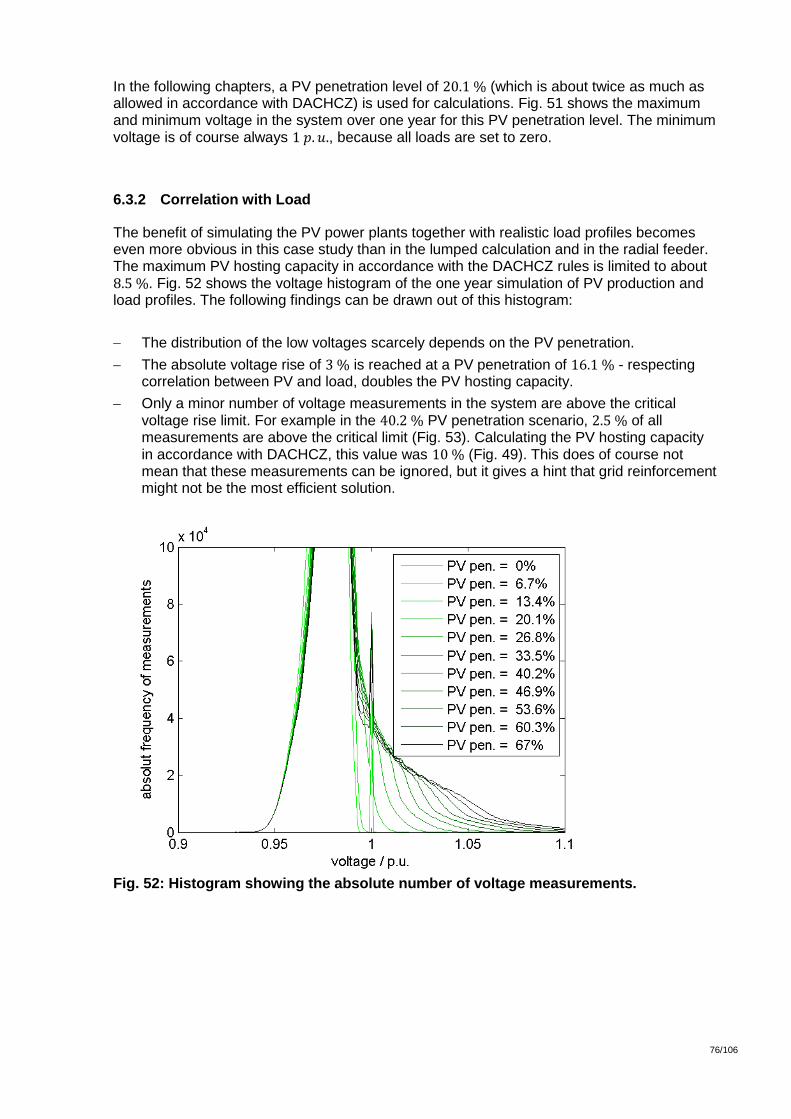
76/106


76

In the following chapters, a PV penetration level of (which is about twice as much as allowed in accordance with DACHCZ) is used for calculations. Fig. 51 shows the maximum and minimum voltage in the system over one year for this PV penetration level. The minimum voltage is of course always , because all loads are set to zero.


The benefit of simulating the PV power plants together with realistic load profiles becomes even more obvious in this case study than in the lumped calculation and in the radial feeder. The maximum PV hosting capacity in accordance with the DACHCZ rules is limited to about . Fig. 52 shows the voltage histogram of the one year simulation of PV production and load profiles. The following findings can be drawn out of this histogram:

The distribution of the low voltages scarcely depends on the PV penetration.

The absolute voltage rise of is reached at a PV penetration of - respecting correlation between PV and load, doubles the PV hosting capacity.

Only a minor number of voltage measurements in the system are above the critical voltage rise limit. For example in the PV penetration scenario, of all measurements are above the critical limit (Fig. 53). Calculating the PV hosting capacity in accordance with DACHCZ, this value was (Fig. 49). This does of course not mean that these measurements can be ignored, but it gives a hint that grid reinforcement might not be the most efficient solution.

Fig. 52: Histogram showing the absolute number of voltage measurements.

77/106


77

Fig. 53: Relative number of voltage measurements under a certain voltage.

Up to a PV penetration of , the loads are the dominant factor for current loading (Fig.

54). The most loaded line is loaded up to even in the no PV scenario. The first line is overloaded only in the PV penetration scenario. Increasing the PV penetration to

, 2 of 162 lines are overloaded.

Fig. 54: Relative current loading of the lines.

These results show that up to a certain extent, PV is a relief for the grid. The investigation of grid losses is one method to evaluate the impact of PV on the grid. Not only the same characteristics but even the same figures are found monitoring grid losses as a function of the PV penetration (Fig. 55): At a penetration level of , the losses are minimised by

78/106


78

almost . This corresponds quite closely to the 1000 households' case in the lumped model investigations.

The total yearly consumption in the case study area is . The grid losses without

PV are about , which corresponds to . If the PV penetration is increased to , the grid losses decrease to which is of the energy supplied to the

loads. The reduced losses of correspond roughly to the energy yield of a PV power plant.

Fig. 55: Additional grid losses caused by PV.

The distribution over the year of the grid losses for the scenario with PV hosting capacity are shown in Fig. 56. The loss reduction is bigger in summer than in winter, both in relative and absolute numbers. The average power dissipation over one year is about

without PV and for the PV hosting capacity scenario.

79/106


79

Fig. 56: Grid loss distribution over the year, given in average power.

Comparing Fig. 57 with Fig. 51 gives a good impression of the voltage damping effects of the loads in the grid. All though loads and solar irradiance are both stochastic and not reliable, the highest voltage in the system was reduced from to

Fig. 57: Maximum and minimum voltage in the DACHCZ simulation with 20.1 % PV penetration over one year.

80/106


80


The PV hosting capacity of the "Luchswiesenstrasse" grid is if the loads are ignored,

and if they are considered. These values are true if the power factor ( ) is equal to one. Decreasing the power factor to ( ) inductive (lagging), the PV hosting

capacity increases by about if loads are used in the simulation. Further decreasing of ( ) to increases the PV hosting capacity by another to (Fig. 58).

In the no load simulation, the beneficial effect of RPC would be even bigger because the loads are already inductive and therefore limit the voltage reduction effect.

Fig. 58: PV hosting capacity and additional PV hosting capacity using RPC.

As the PV penetration can be increased if RPC is used, the current loading of the lines should be monitored. Fig. 59 shows the respective relative current loadings for six scenarios. Only in the last scenario (PV penetration of corresponding to the maximum PV hosting capacity using RPC and correlation of PV and loads), one line is slightly overloaded ( ).

81/106


81

Fig. 59: Relative current loading for the maximum PV hosting capacity of six scenarios using RPC.


From the PV hosting capacity per household rises to if the APC ratio is limited to . The energy losses are slightly higher than in this case (Fig. 60).

Fig. 60: PV hosting capacity and energy losses depending on APC ratio.

Increasing the PV penetration using APC does however not change the maximum relative current loading in the grid (Fig. 61). This means that the maximum thermal stress of the

82/106


82

cables only depends on the AC power of the PV power systems and not on their nominal DC power.

Fig. 61: Relative current loading using APC.


As the roof orientations and correspondingly the orientation of the PV power systems is given in the case study, this investigation is not pursued.

6.3.6 Storage

Both storage systems and DSM are not investigated in the case study. Too many assumptions would have been necessary, and the results would have been specific to these assumptions rather than for the concept itself.


With the same reasons as for the storage method (section 6.3.6), DSM is not investigated in this study.


The benefit in increasing the PV hosting capacity of an LVDG using OLTC is shown in section 6.1.8. Fig. 62 shows the voltage profile (minimum and maximum system voltage) with

and without OLTC for a PV penetration scenario of . The OLTC operation scheme of this simulation is not optimised but simply cuts overvoltages and raises undervoltages.

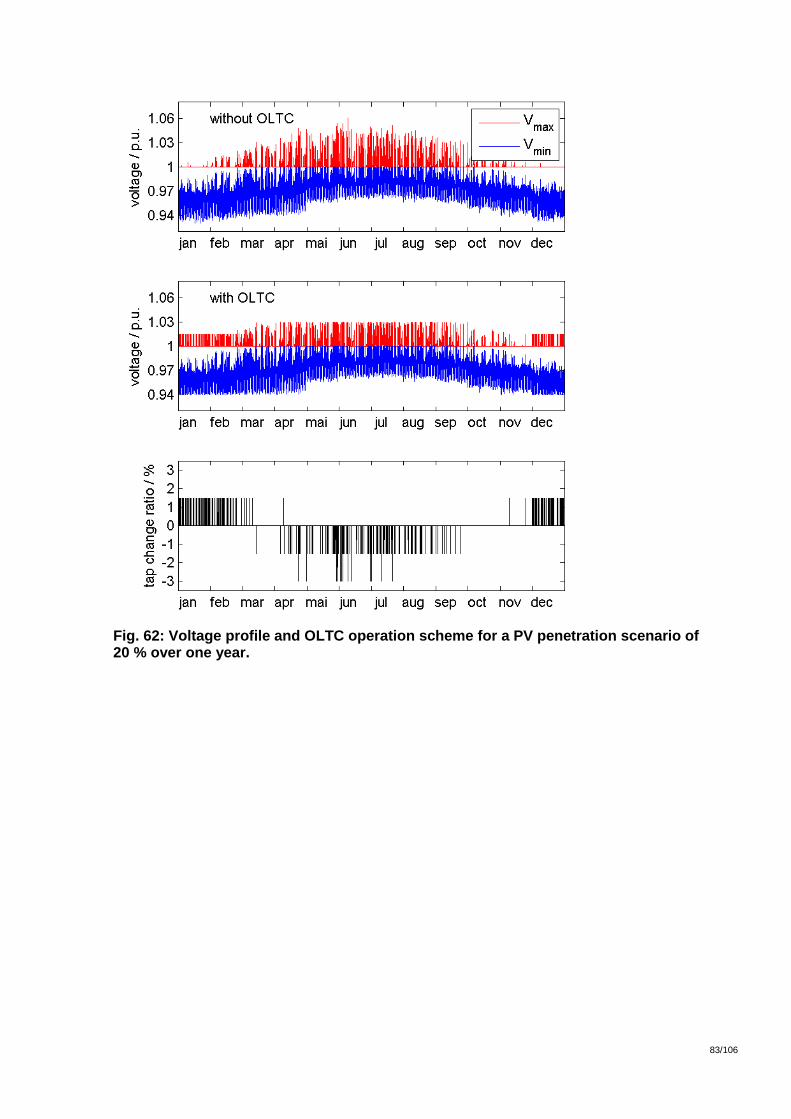
83/106


83

Fig. 62: Voltage profile and OLTC operation scheme for a PV penetration scenario of 20 % over one year.

84/106


84

6.4 Monte Carlo Results

All previous PV hosting capacities are derived using worst case scenarios: The highest voltage peak over one year defines the PV hosting capacity of a network.

With Monte Carlo simulations a more realistic view on the occurrence of these worst case scenarios can be obtained. Fig. 21 compares the PV hosting capacity of a simple lumped model network using the DACHCZ approach with the correlation approach. The derivation of the PV hosting capacity with the DACHCZ approach is repeated in this chapter using 100 simulations of the 21st June (Fig. 63).

The maximum voltage rise within a day is still used to compute the PV hosting capacity of the grid, but as 100 days are simulated, the worst case within a day differs from day to day. However, Fig. 63 shows clearly that most results are rather close together and go in line with Fig. 21. Using the DACHCZ approach, conventional simulations (non-Monte Carlo) are therefore quite significant.

Fig. 63: Results of Monte Carlo Simulation of the 21st June using the DACHCZ approach and the lumped model (chapter 6.1).

Assuming the minimum PV hosting capacity found in Fig. 63 and simulating 1000 summer days with this hosting capacity, the distribution of maximum voltages in Fig. 64 is found. Even if loads in the grid are ignored, the critical voltage is unlikely to occur.

85/106


85

Fig. 64: Maximum voltage during the 21st June (1000 days are simulated), no load.

Critical voltages are even less likely if the loads in the grid are no longer ignored. While the correlation between a PV power plant and one household still gives similar results to the no load case (Fig. 65), only ten households shift the maximum daily voltage from towards .

While in section 6.1.2 an additional PV hosting capacity of was predicted, Fig. 65 shows that most of the time the absolute voltage rise using the DACHCZ approach in a grid

with 100 households does not even exceed . The PV penetration could therefore be more than doubled without causing too many violations.

The data of Fig. 65 is listed in Tab. 3 in absolute values. The total number of simulated days is . The highest voltage simulated in the 100 household case is , but it

occurs twice in 1000 midsummer days. In of all days the voltage stays below .

Clearly the remaining of all days with voltages must also be dealt with. This could be done with a smart APC approach (section 5.4.2), limiting the power output only in those moments when PV production is high and the loads are low.

Fig. 28 (energy recovery using smart APC with an APC ratio of ) reinforces the

message of Fig. 65: The more households that are connected to the grid, the less energy is lost using the presented smart APC approach.

86/106


86

Fig. 65: Maximum voltage during the 21st June (1000 days are simulated), with household loads.

Voltage (p.u.) NrHH 1

1.0

01

1.0

02

1.0

03

1.0

04

1.0

05

1.0

06

1.0

07

1.0

08

1.0

09

1.0

10

1.0

11

1.0

12

1.0

13

1.0

14

1 0 0 0 0 1 5 0 0 0 0 0 9 16 21 15

2 0 0 0 0 2 4 0 0 0 0 4 13 16 19 10

5 0 0 0 1 2 3 0 0 1 2 9 20 18 20 25

10 0 0 0 3 2 1 0 2 5 18 19 20 17 21 15

20 0 2 2 2 1 7 11 18 13 20 20 18 10 8 13

50 7 4 9 12 10 25 22 24 17 12 7 15 23 64 94

100 109 22 16 26 52 63 87 99 125 120 107 80 47 22 15

200 588 124 94 76 51 30 18 8 4 0 2 2 3 0 0

500 997 2 1 0 0 0 0 0 0 0 0 0 0 0 0

1000 1k 0 0 0 0 0 0 0 0 0 0 0 0 0 0

Voltage (p.u.) NrHH 1

.01

5

1.0

16

1.0

17

1.0

18

1.0

19

1.0

20

1.0

21

1.0

22

1.0

23

1.0

24

1.0

25

1.0

26

1.0

27

1.0

28

1.0

29

1.0

30

1 21 6 18 16 21 1 3 27 185 285 123 82 84 42 6 13

2 21 17 19 8 18 1 8 54 282 214 103 89 64 16 9 9

5 13 13 12 12 3 11 61 254 247 100 89 47 24 7 4 2

10 9 8 11 7 14 126 280 203 91 62 39 13 11 3 0 0

20 11 13 30 116 233 220 127 53 27 15 6 2 2 0 0 0

50 181 177 148 89 35 16 4 3 2 0 0 0 0 0 0 0

100 6 2 2 0 0 0 0 0 0 0 0 0 0 0 0 0

200 0 0 0 0 0 0 0 0 0 0 0 0 0 0 0 0

500 0 0 0 0 0 0 0 0 0 0 0 0 0 0 0 0

1000 0 0 0 0 0 0 0 0 0 0 0 0 0 0 0 0

Tab. 3: Absolute number of days with the corresponding voltage (data of histogram in Fig. 65, N=1000).

87/106


87

7 Conclusion

In this report the maximum PV hosting capacity of a low voltage distribution grid has been investigated. Although there are several results which only apply to specific grids and network topologies, a range of general conclusions can be drawn which are likely to apply to most grids:

Considering the loads in the grid increases the PV hosting capacity from a few per cent for a single household to more than 50 % for a large number of households.

Reactive power control can be a powerful way to integrate more PV in the LV distribution grid – however not in all situations. Whether RPC increases the PV hosting capacity or not depends on the specific grid topology – mainly on the ratio between grid resistance and grid reactance.

Active power curtailment is able to solve almost every LV grid integration issue, but it is a waste of energy. The smart way to deal with APC is to implement a whole range of measures which reduce the average power fed into the grid (considering the loads, using DSM or using storage), and to cut the remaining peaks with APC. The PV hosting capacity of an LV grid can therefore easily be doubled and only a few per cent of energy is lost, if any at all.

The application of different orientations of PV systems is not too promising. An east-west-facing system reduces the power peak significantly, but the energy yield is reduced by about the same percentage. The amount of energy which can be fed into the distribution grid is thereby not changed a lot, unless PV module tilt angles of more than 50 % are applied, which is normally not economic.

Whatever problem could not be solved employing the above measures can be solved using storage systems. Four hours of nominal operation stored in local storage increases the PV hosting capacity of an LVDG to more than 200 %.

Depending on the loads which can be switched dynamically, demand side management may or may not be a powerful tool. Even DSM cannot guarantee a certain load at a certain point in time. The best way to use DSM is therefore in a combination with a smart APC algorithm.

On load tap change transformers could double the PV hosting capacity of the LVDG mainly in rural areas where current loadings of the lines are not an issue but voltage drop is significant. But municipal areas are not excluded either. It is however necessary to simulate the whole LVDG to assess the applicability of OLTC transformers.

25 % PV penetration minimises grid losses by 5 % to 20 % depending on the number of households which are connected to the grid. The more households, the bigger the benefit. However, the penetration which minimises the losses is 25 % in all cases.

88/106


88

8 Outlook

8.1 Measurement and Analysis of Load Patterns

In November 2012, ewz started gathering field measurements of load consumption data with a temporal resolution of one minute for 53 customers. The measurements will be analysed and used to calibrate the load profile generator (section 4.4). Certain simulations will be recomputed depending on the deviations between the randomised load profiles used in this project and the measured load profiles.

The measurements will be presented in a separate report.

8.2 Dissertation

This project is the main part of the dissertation of the principal author (Christof Bucher). Within a year of the publication of this report, the publication of the dissertation is planned, including the work described in chapter 8.1.

8.3 Further Research

As a next step, the results of this project should be verified by case studies. Independent of this project, many case studies are already on-going, and certain results have already been verified (for example the loss minimisation at a PV penetration of 25 % by Danfoss [47]).

The conclusions of this project show that regarding LVDG, a large amount of our electricity needs can be covered by PV systems. However, significantly higher barriers might occur regarding not only the LVDG but the whole electricity grid. Frequency stability, control reserve or storage requirements are issues which might be affected considerably if a lot of PV will be introduced into the electricity grid – even if it will be connected to the LVDG. Measures presented in this report should therefore in future not only be optimised for the LVDG, but for the whole electricity supply system.

89/106


89

9 References

9.1 Papers and Reports Published within this Project

[1] Christof Bucher, Göran Andersson, Generation of Domestic Load Profiles – an Adaptive Top-Down Approach, proceedings of PMAPS 2012, Istanbul, Turkey, 2012.

[2] Christof Bucher, Jethro Betcke, Göran Andersson, Benoît Bletterie, Lukas Küng, "Simulation of Distribution Grids with Photovoltaics by Means of Stochastic Load Profiles and Irradiance Data", in proceedings of the 27th European Photovoltaic Solar Energy Conference and Exhibition, Frankfurt, Germany, 2012, pp. 3795 - 3800.

[3] Christof Bucher, Jethro Betcke, Göran Andersson, "Effects of Variation of Temporal Resolution on Domestic Power and Solar Irradiance Measurements", Powertech 2013, Grenoble, France, 16-20 June 2013.

[4] Christof Bucher, Göran Andersson, Lukas Küng, "Increasing the PV Hosting Capacity of Distribution Power Grids – a Comparison of Seven Methods", in proceedings of the 28th European Photovoltaic Solar Energy Conference and Exhibition, Paris, France, 2013.

[5] Jethro Betcke, Jan Kühnert, Thomas Scheidtsteger, Development and Validation of the DiGASP Weather Generator, Technical report, Carl von Ossietzky University of Oldenburg Energy and Semiconductor Research Laboratory Energy Meteorology group, August 2013.

[6] In press: Benoît Bletterie et al., Implementation of local voltage control by PV inverters in LV networks – Considerations on the parameterisation and stability issues. Technical report, AIT, Vienna, Austria, December 2013.

9.2 General References

[7] EPIA, "Global Market Outlook for Photovoltaics 2013-2017", European Photovoltaic Industry Association (EPIA), 2013, Brussels – Belgium.

[8] Finlay Colville, "The PV industry at the end of 2012: reasons to be fearful", Solarbuzz. Available at: http://www.solarbuzz.com/sites/default/files/solarbusiness_focus_v5.pdf

[9] Schneider Electric, "Planungskompendium Energieverteilung unter Berücksichtigung von IEC, EN, HD, DIN VDE", Hüthig Verlag, 2007, Heidelberg, Germany.

[10] "The European Electricity Grid Initiative (EEGI)", entsoe and EDSO, Version V2, May 2010, Available at http://www.smartgrids.eu/documents/EEGI/EEGI_Implementation_plan_May%202010.pdf

[11] "Weissbuch Smart Grid", Verein Smart Grid Schweiz VSGS, February 2013. Available at: http://www.smartgrid-schweiz.ch/media/files/Weissbuch_Smart_Grid.pdf

[12] Marktmodell für die elektrische Energie – Schweiz. Grundsatzdokument zur Regelung der zentralen Aspekte der Organisation des Strommarktes Schweiz. Verband Schweizerischer Elektrizitätsunternehmen VSE, Aarau, Switzerland, 2009. Available at: http://www.strom.ch/de/dossiers/strommarkt/branchendokumente.html

[13] EPIA, Competing in the Energy Sector - Preliminary Project Results, European Photovoltaic Industry Association (EPIA), Paris, March 2011.

[14] Various grid levels transport electricity, swissgrid. Available at: http://www.swissgrid.ch/swissgrid/en/home/grid/transmission_system/grid_levels.html

[15] R. Baumann et al., “Metering Code Schweiz”, Technische Bestimmungen zu Messung und Messdatenbereitstellung, Verband Schweizerischer Elektrizitätsunternehmen VSE/AES, Aarau, Switzerland, 2011.

http://www.solarbuzz.com/sites/default/files/solarbusiness_focus_v5.pdf

http://www.smartgrids.eu/documents/EEGI/EEGI_Implementation_plan_May%202010.pdf

http://www.smartgrids.eu/documents/EEGI/EEGI_Implementation_plan_May%202010.pdf

http://www.smartgrid-schweiz.ch/media/files/Weissbuch_Smart_Grid.pdf

http://www.strom.ch/de/dossiers/strommarkt/branchendokumente.html

http://www.swissgrid.ch/swissgrid/en/home/grid/transmission_system/grid_levels.html

90/106


90

[16] P. Hallberg, “Final Guidelines of Good Practice on Regulatory Aspects of Smart Metering for Electricity and Gas”, European Regulators Group for Electricity and Gas, Council of European Energy Regulators ASBL, Brussels, February 2011.

[17] A. Wright, S. Firth, “The nature of domestic electricity loads and effects of time averaging on statistics and on-site generation calculations”, Institute of Energy and Sustainable Development, De Montfort University, Leicester, UK, 2006.

[18] J. Widén, E. Wäckelgård, J. Paatero, P. Lund, “Impacts of different data averaging times on statistical analysis of distributed domestic photovoltaic systems”, in Solar Energy, March 2010, Vol. 84, No. 3., pp. 492-500.

[19] Voltage characteristics of electricity supplied by public distribution networks, EN 50160:2010, March 2010.

[20] A. Einfalt et al., “Development of concepts for ADRES Autonomous Decentralized Regenerative Energy Systems”, in Austrian Climate and Energy Fund, 1. AS, Project no: 815674, final report, Vienna 2011.

[21] J. Zico Kolter, M. J. Johnson, “REDD: A public data set for energy disaggregation research”, in proceedings of the SustKDD workshop on Data Mining Applications in Sustainability, 2011.

[22] M. Weiss, A. Helfenstein, F. Mattern, T. Staake, “Leveraging smart meter data to recognize home appliances”, in proceedings of the IEEE International Conference on Pervasive Computing and Communications (PerCom 2012), pp. 190-197, Lugano, Switzerland, March 2012.

[23] J. Kühnert, T. Behrendt, E. Lorenz, A. Hammer, J. Betcke, D. Heinemann, “Spectral and reflection effects for different PV technologies based on ground measurements and satellite data”, in proceedings of 26th EUPVSEC Hamburg, 5. - 9. September 2011.

[24] G. Andersson, “Modelling and Analysis of Electric Power Systems”, EEH - Power Systems Laboratory, ETH Zürich, September 2009.

[25] G. Bartak, H. Holenstein, J. Meyer, “Technical Rules for the Assessment of Network Disturbances”, VEÖ Austria, VSE Switzerland, CSRES Czech Republic, VDN Germany, 2nd edition, 2007.

[26] H. Suehrcke, P.G. MCCormick, “The frequency distribution of instantaneous insolation values”, in Solar Energy 40, pp. 413-422, 1988.

[27] A. Woyte, R. Belmans, J. Nijs, “Fluctuations in instantaneous clearness index: Analysis and statistics”, in Solar Energy 81, pp. 195-206, 2007.

[28] R. D. Zimmerman, C. E. Murillo-Sánchez, and R. J. Thomas, Matpower: Steady-State Operations, Planning and Analysis Tools for Power Systems Research and Education, Power Systems, IEEE Transactions on, vol. 26, no. 1, pp. 12{19, Feb. 2011.

[29] METEONORM V6.1, www.meteotest.ch, Meteotest, Fabrikstrasse 14, Bern, Switzerland.

[30] Ian Richardson, Murray Thomson, David Infield, A high-resolution domestic building occupancy model for energy demand simulations, 2008, Centre for Renewable Energy Systems Technology, Loughborough University, Leicestershire, England.

[31] J. Dickert, P. Schegner, Residential Load Models for Network Planning Purposes, 2010, Technische Universität Dresden, Germany.

[32] R. Herman, C. Gaunt, S. Heunis, Voltage drop effects depending on different customer feeder connections, 1998, South African Institute of Electrical Engineers.

[33] ÜZ Lülsfeld, Standardisierte Lastprofile, www.uez.de/Standardisierte_Lastprofile.html, accessed March 7 2012.

[34] Marianne M. Armstrong, Mike C. Swinton, Hajo Ribberink, Ian Beausoleil-Morrison, Jocelyn Millette, Synthetically derived profiles for representing occupant-driven electric loads in Canadian Housing, 2009, National Research Council Canada, Ottawa.

http://www.meteotest.ch/

http://www.uez.de/Standardisierte_Lastprofile.html,

http://www.uez.de/Standardisierte_Lastprofile.html,

91/106


91

[35] Fintan J. McLoughlin, Aidan Duffy, Michael Conlon, The Generation of Domestic Electricity Load Profiles through Markov Chain Modelling, 2010, Department of Civil and Structural Engineering, School of Civil and Building Services, Dublin, Ireland.

[36] Frank Jay, J. A. Goetz, IEEE Standard Dictionary of Electrical and Electronic Terms, 3rd ed., 1984, The Institute of Electrical and Electronics Engineers, New York, USA.

[37] A. Hammer, D. Heinemann, C. Hoyer, R. Kuhlemann, E. Lorenz, R. Müller, H. Beyer, Solar energy assessment using remote sensing technologies, Remote Sensing of Environment, vol. 86, pp.423-432, 2003.

[38] A. Skartveit, J.A. Olseth, The probability density and autocorrelation of short-term global and beam irradiance, Solar Energy, vol. 49, no. 6, pp 477-487, 1992.

[39] D. Dumortier, Modelling global and diffuse horizontal irradiances under cloudless skies with different turbidities, daylight II final report. Technical Report jou2-crt92-0144, CNRS-ENTPE, Vaulx-en-Velin, France, 1995.

[40] G.C. Calafiore, M.C. Campi, The Scenario Approach to Robust Control Design, Politecnico di Torino, IEEE Transactions on Automatic Control, June 2006.

[41] Gerhard Bartak, Hansjörg Holenstein, Jan Meyer, Technical Rules for the Assessment of Network Disturbances, 2nd ed., Austria, Germany, Czech Republic, Switzerland, 2007.

[42] VDE-AR-N 4105, Technical requirements for the connection to and parallel operation with low-voltage distribution networks, VDE VERLAG GMBH, Berlin, Germany, 2011.

[43] Georg Kerber, Rolf Witzmann, Hannes Sappl, Voltage limitation by autonomous reactive power control of grid connected photovoltaic inverters, Compatibility and Power Electronics, 2009. CPE '09, pp.129-133, 20-22 May 2009.

[44] Reinaldo Tonkoski, Luiz A. C. Lopes, Tarek H. M. El-Fouly, Droop-based active power curtailment for overvoltage prevention in grid connected PV inverters, Industrial Electronics (ISIE), 2010 IEEE International Symposium, vol., no., pp.2388-2393, 4-7 July 2010.

[45] Adrian Constantin, Radu Dan Lazar, Søren Bækhøj Kjær, "Voltage control in low voltage networks by Photovoltaic Inverters, Case-study Bornholm", Danfoss Solar Inverters A/S, Denmark, December 2012.

[46] Rafael Amaral Shayani, Marco Aurélio Gonçalves de Oliveira, Photovoltaic Generation Penetration Limits in Radial Distribution Systems, Power Systems, IEEE Transactions on, vol.26, no.3, pp.1625-1631, Aug. 2011.

[47] Dr. Søren Bækhøj Kjær et al., Voltage Control in Low Voltage Networks by Photovoltaic Inverters – PVNET.DK, 28th EUPVSEC 2013 Paris, Danfoss Solar Inverters, Sønderborg, Denmark.

[48] Yannick Riesen, Pengcheng Ding, Samuel Monnier, Nicolas Wyrsch and Christophe Ballif, "Peak Shaving Capability of Household Grid-Connected PV System with local Storage: A Case Study", Ecole Polytechnique Fédérale de Lausanne (EPFL), Institute of Microengineering (IMT), Photovoltaics and Thin Film Electronics Laboratory Neuchatel, in proceedings of the 28th European Photovoltaic Solar Energy Conference and Exhibition, Paris, France, 2013.

[49] Christopher Williams, Jann Binder, Michael Danzer, Frank Sehnke, Martin Felder, "Battery Charge Control Schmemes for Increased Grid Compatibility of Decentralized PV Systems", Zentrum für Sonnenenergie- und Wasserstoff-Forschung Baden-Württemberg, in proceedings of the 28th European Photovoltaic Solar Energy Conference and Exhibition, Paris, France, 2013.

[50] Evangelos Vrettos, Andreas Witzig, Roland Kurmann, Stephan Koch and Göran Andersson, "Maximizing Local PV Utilization using Small-Scale Batteries and Flexible Thermal Loads", Power Systems Laboratory, ETH Zürich, in proceedings of the 28th European Photovoltaic Solar Energy Conference and Exhibition, Paris, France, 2013.

92/106


92

[51] Martin Stötzer, Phillip Gronstedt, Zbigniew Styczynski, Demand Side Management Potential A Case Study for Germany, CIRED, 21st International Conference on Electricity Distribution, Frankfurt, June 2011.

[52] I. Rohmund, B. Kester, Demand Side Management Potential Study, EnerNOC Utility Solutions Consulting, CA, August 2013.

[53] Kathrin Degen, Charles Efferson, Fabian Frei, Lorenz Götte, Rafael Lalive, Smart Metering, Beratung oder Sozialer Vergleich. Was beeinflusst den Elektrizitätsverbrauch? ewz-Studie Smart Metering. Zusammenfassung der Resultate. ewz Zürich, Universität Lausanne, Universität Zürich, Switzerland, July 2013.

[54] Johannes Brantl, New Challenges for DSO, E.ON Bavaria, IEA PVPS Task 14 meeting, Kassel, 2012.

[55] Reinaldo Tonkoski, Luiz A. C. Lopes, Tarek H. M. El-Fouly, Coordinated Active Power Curtailment of Grid Connected PV Inverters for Overvoltage Prevention, Sustainable Energy, IEEE Transactions on, vol.2, no.2, pp.139-147, April 2011.

[56] Chia-Hung Lin, Wei-Lin Hsieh, Chao-Shun Chen, Cheng-Ting Hsu, Te-Tien Ku, Optimization of Photovoltaic Penetration in Distribution Systems Considering Annual Duration Curve of Solar Irradiation, Power Systems, IEEE Transactions on, vol.27, no.2, pp.1090-1097, May 2012.

[57] Ruifeng Yan, Tapan Kumar Saha, Investigation of Voltage Stability for Residential Customers Due to High Photovoltaic Penetrations, Power Systems, IEEE Transactions on, vol.27, no.2, pp.651-662, May 2012.

[58] Ian Richardson, Graeme Hodgson, Murray Thomson, David Infield, Alice Delahunty, Simulation of high-resolution domestic electricity demand based on a building occupancy model and its applicability to the study of demand side management, Centre for Renewable Energy Systems Technology, Loughborough University, Leicestershire, England, 2008.

[59] R. D. Zimmerman, C. E. Murillo-Sánchez, and R. J. Thomas, Matpower: Steady-State Operations, Planning and Analysis Tools for Power Systems Research and Education, Power Systems, IEEE Transactions on, vol. 26, no. 1, pp. 12{19, Feb. 2011.

[60] Almut Kirchner et al., Analyse des schweizerischen Energieverbrauchs 2000-2006 nach Verwendungszwecken, Swiss Federal Office of Energy, Bern, Switzerland, April 2008.

[61] Alois Huser, Thomas Grieder, Geräteausstattung und Stromverbrauch von Schweizer Haushalten, Bulletin SEV / VSE 4/06, Aarau, Switzerland, 2006.

[62] Stephan Koch, Johanna L. Mathieu and Duncan S. Callaway, Modeling and Control of Aggregated Heterogeneous Thermostatically Controlled Loads for Ancillary Services, 17th Power Systems Computation Conference, Stockholm, Sweden, 2011.

[63] Families, households – Data, indicators. Distribution of households according to type, Swiss Federal Office of Energy, Bern, Switzerland, www.bfs.admin.ch/bfs/portal/en/index/themen/01/04/blank/key/haushaltstypen.html, accessed July 18 2012.

9.3 Dissemination: Presentations and Articles Hold and Published by Christof Bucher

[64] Oral presentation: "Auswirkungen eines hohen Photovoltaikanteils auf das Niederspannungsnetz", national PV session Switzerland, 23th March 2012, Baden, Switzerland.

http://www.bfs.admin.ch/bfs/portal/en/index/themen/01/04/blank/key/haushaltstypen.html,

http://www.bfs.admin.ch/bfs/portal/en/index/themen/01/04/blank/key/haushaltstypen.html,

93/106


93

[65] Oral presentation: " Wie viel Photovoltaik (PV) verträgt ein Verteilnetz ohne Netzausbau?", Energie-Apéro Aargau, October 2013, three presentations in Baden, Lenzburg and Aarau, Switzerland.

[66] Oral presentation: "Distribution Grid Analysis and Simulation with Photovoltaics (DiGASP)", 22th January 2013, Oldenburg, Germany.

[67] Visual presentation: "Leistungsreduktion bei PV-Anlagen. Energieverschwendung oder günstige Massnahme zur besseren Netzintegration?", national PV session Switzerland, 11th March 2013, Basel, Switzerland.

[68] Oral presentation: " Einbindung dezentrale Erzeugung – Wann muss ausgebaut werden?", Innovationsforum Energie, 15th March 2013, Zürich.

[69] Oral presentation: " Comparison of 7 measures to integrate PV in the low voltage grid, using stochastic irradiance data", IEA PVPS & SHC workshop, PVSEC 2013, 1st October 2013, Paris, France.

[70] Oral presentation: " Distribution Grid Analysis and Simulation with Photovoltaics (DiGASP) ", ewz, 22th October 2013, Zürich, Switzerland.

[71] Oral presentation: " Methoden zur Erhöhung des Solarstromanteils im Niederspannungsnetz ", Elektrizitätswerke Schönau (EWS), 8th November 2013, Schönau, Germany.

[72] Article (in press): " Wie viel Solarstrom verträgt das Niederspannungsnetz?", Bulletin VSE/electrosuisse, spring 2014.

[73] Dissertation (in press): " Distribution Grid Analysis and Simulation with Photovoltaics (DiGASP) ", spring 2014, Zürich, Switzerland.

94/106


94

Appendix

A: Optimised APC

Whenever APC was used in this project, identical parameters were used for all PV power plants in a network. In this section parameters are chosen individually for every plant. With an optimisation algorithm the APC losses are minimised.

1. Definitions

Homogeneous APC: Homogeneous APC in a power grid means that only one single APC ratio is applied to all PV power systems in the grid.

APC loss: The lost / curtailed solar energy is denoted as "APC loss".

APCn: APC ratio of node n.

Single line feeder: The test feeder used in this document is a single line with N nodes:

2. Optimisation Problem Formulation

The optimum APC ratios of different PV power systems in order to minimise APC losses are to be found.

Minimise:

∑

(27)

Subjected to:

(28)

The following parameters have been used in this document:

The optimisation problem is formulated in Matlab using the fmincon-function and the

active-set-algorithm.

n=2 n=1 n=3

grid

U1, APC1

n=N

U0 =1pu

U2, APC2

Un, APCn

UN, APC

N

95/106


95

3. Optimisation Results

Both the homogeneous and the optimised APC algorithm limit the maximum voltage rise to the given reference value of 3 % (here shown as 1.03 per unit), see Fig. 66. However in the optimised APC algorithm, the PV power plants at the remote network nodes must limit their AC power much more than those plants close to the feeder.

In a ten node network hosting roughly twice as much PV power as possible without APC, the APC losses are reduced from 8.9 % in the homogeneous APC approach to 7.2 % in the optimised approach. This is a difference of roughly 20 %.

Fig. 66: APC optimisation results. Comparison of homogeneous and optimised APC ratios.

Depending on the amount of PV which is hosted in the single line feeder, different APC ratios must be applied. Fig. 67 shows various APC ratios for different PV hosting scenarios. 100 % PV penetration denotes in this case the maximum amount of PV that can be hosted by the single feeder without any APC (APC ratio = 1 for all PV plants).

96/106


96

Fig. 67: APC ratios for different PV penetration scenarios. 100 % PV (constant APC ratio of 1) stands for the maximum PV power which can be hosted without any APC taking place.

Looking at the APC losses, a typical APC loss curve is found (Fig. 68). For every PV penetration scenario, the optimal APC algorithm reduces the APC losses by 15 % - 20 %.

The relative loss reduction obviously does not depend much on the PV penetration, but it depends on the length of the feeder (Fig. 69). The shorter the feeder, the smaller is the loss reduction. There is however a saturation of the loss reduction which starts at about the ten node feeder: The loss reduction cannot augment much more than 20 %.

Fig. 68: APC losses for homogeneous and optimal APC ratios depending on the PV penetration.

97/106


97

Fig. 69: Relative reduction of APC losses using optimised APC depending on the feeder length. The range of PV penetration in the feeder is between 100 % and 280 % of the PV hosting capacity.

Using APC can significantly increase the PV hosting capacity of a distribution power grid, but it causes losses in energy yield. These losses can be reduced by 15 % - 20 % applying optimum APC ratios. However, using optimum APC ratios the APC losses vary greatly from node to node. Close to the feeder, only minimal losses have to be considered, whereas the losses remote from the feeder are considerably higher.

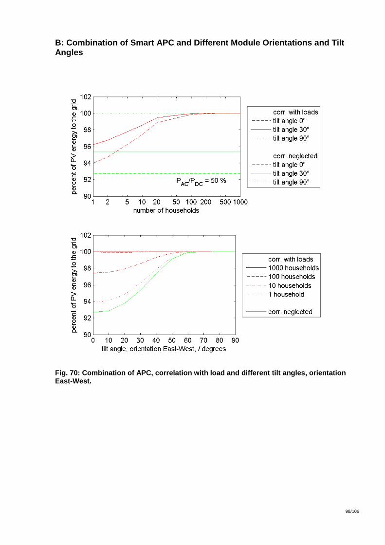
98/106


98

B: Combination of Smart APC and Different Module Orientations and Tilt Angles

Fig. 70: Combination of APC, correlation with load and different tilt angles, orientation East-West.

99/106


99

Fig. 71: Combination of APC, correlation with load and different tilt angles, orientation East.

100/106


100

Fig. 72: Combination of APC, correlation with load and different tilt angles, orientation South.

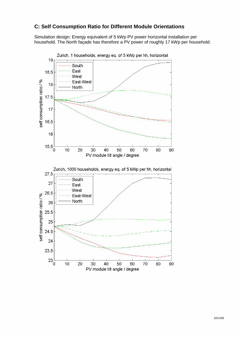
101/106


101

C: Self Consumption Ratio for Different Module Orientations

Simulation design: Energy equivalent of 5 kWp PV power horizontal installation per household. The North façade has therefore a PV power of roughly 17 kWp per household.

102/106


102

Simulation design: Maximum PV output power corresponds to household peak load. The horizontal installation of a single household system has 10 kWp, the North façade of the single household roughly 37 kWp.

103/106


103

Simulation design: Constant installed power. Every household has 5 kWp.

104/106


104

D: Self Sufficiency Ratio for Different Module Orientations

Simulation design: Energy equivalent of 5 kWp PV power horizontal installation per household. The North façade has therefore a PV power of roughly 17 kWp per household.

105/106


105

Simulation design: Maximum PV output power corresponds to household peak load. The horizontal installation of a single household system has 10 kWp, the North façade of the single household roughly 37 kWp.

106/106


106

Simulation design: Constant installed power. Every household has 5 kWp.

DiGASP Distribution Grid Analysis and Simulation with ...

Documents

Transcript of DiGASP Distribution Grid Analysis and Simulation with ...