Differential Optical Absorption Spectroscopy of … Optical Absorption Spectroscopy of Trace Gas...

Differential Optical Absorption Spectroscopy of Trace Gas Species and Aerosols in the

Upper Ohio River Valley

Dissertation

Presented in Partial Fulfillment of the Requirements for the Degree Doctor of Philosophy

in the Graduate School of The Ohio State University

By

Christopher Paul Beekman, B.S.

Environmental Science Graduate Program

The Ohio State University

2010

Dissertation Committee:

Heather C. Allen, Advisor

Catherine A. Calder

Bryan G. Mark

Franklin W. Schwartz

Copyright by

Christopher P. Beekman

2010

ii

Abstract

In this research, it is hypothesized that recently developed theoretical considerations of

atmospheric radiative transfer in horizontally in-homogeneous atmospheres can be applied to the

remote measurement of anthropogenic plumes. To this end, a MAX-DOAS spectrometer,

designed around a B&W-TEK BTU142 spectrometer was constructed and characterized. It was

found that the MAX-DOAS spectrometer has a measured resolution of 0.282 nm, and a noise

level of 178 counts at 75% pixel saturation, sufficient to resolve accurately the absorptions of

important atmospheric species, including SO2, NO2, HCHO, and O4. The theory of MAX-DOAS

spectral analysis was examined in detail, in particular the processing of reference absorption

cross-section spectra for use in regression analyses of scattered solar radiation. For the purposes

of inversion, optimal estimation software was designed and investigated for suitability in

retrieving vertical profiles of atmospheric species. This software is shown to perform well under

conditions of both typical and non-typical noise levels using synthetic spectral data and known

profiles of three atmospheric species. Furthermore, an extensive examination of the residuals of

DOAS spectral analysis was performed, to validate the assumption of normally distributed errors

in the inversion process. Investigated methodologies were applied to spectral data collected over

nine days in 2008 in the Upper Ohio River Valley. Aerosol extinction coefficient profiles were

successfully retrieved, with an average peak value of 0.549 km-1. For the same measurement

period, in-plume measurements of SO2 and NO2 concentration from a coal-fired power plant were

conducted using recently developed methodologies to account for in-plume solar radiative

transfer effects.

iii

Dedication

Dedicated to my wife, Gina, who has been a bottomless well of love and patience, and to

my son, Troy Benjamin, for providing me with all the motivation I could ever need.

iv

Acknowledgements

My sincerest thanks to Dr. Catherine A. Calder and Dr. Radu Herbei of the Statistics

Department of The Ohio State University, for their input and attention to detail

concerning the spectral analysis portion of this research and the development of the

Markov Chain Monte Carlo inversion of atmospheric profiles, the subject of a future

paper. Additionally, I thank Gerald Allen and Dr. Franklin Schwartz for their assistance

in the mapping portions of this dissertation.

v

Vita

1998………………………………………………………………..Shadyside High School

2002………………….....................................B.S. Chemistry and Environmental Science,

Muskingum College

2004 to present……………………………………………...Graduate Teaching Associate,

Department of Chemistry, The Ohio State University

Publications

L. F. Voss, M. F. Bazerbashi, C. P. Beekman, C. M. Hadad, and H. C. Allen, “Oxidation

of oleic acid at air/liquid interfaces.” Journal of Geophysical Research-Atmospheres,

112, 2007.

C. P. Beekman and William J. Mitsch, “Soil Characteristics in a bottomland hardwood

forest five years after hydrologic restoration.” William H. Schiermeier Olentangy River

Wetland Research Park at The Ohio State University Annual Report 2005, 2006.

Fields of Study

Major Field: Environmental Science Graduate Program

vi

Table of Contents

Abstract……………………………………………………………………………………ii

Dedication………………………………………………………………………………...iii

Acknowledgements……………………………………………………………………….iv

Vita…………………………………………………………………………………...........v

List of Figures……………………………………………………………………………..x

List of Tables……………………………………………………………………………xix

Chapter1: Introduction………...…………………………………………………………..1

Chapter 2: Important Tropospheric Chemistries…………………………………………..7

2.1: Introduction to Relevant Tropospheric Chemistry…………………………...7

2.2: The HOx, NOx, and O3 cycles………………………………………………...7

2.3: Tropospheric Formaldehyde…………………………...……………………11

2.4: Sulfur Dioxide Chemistry…………………………………………………...12

Chapter 3: Structure and Physics of the Atmosphere……………………………………16

3.1: Introduction to Atmospheric Structure and Physics………………………...16

3.2: Delineation of Atmospheric Regions……....………………....……………..16

3.3: Solar Radiation and Radiative Transfer……………………………………..20

vii

3.4: Mathematical Description of Atmospheric Scattering………………………22

3.5: Absorption by Atmospheric Gases………………………………………….24

3.6: Radiative Transfer Modeling………………………………………………..25

3.6a: MCARaTS…………………………………………………………26

3.6b: SCIATRAN………………………………………………………..27

Chapter 4: Instrumentation………………………………………………………………29

4.1: Introduction………………………………………………………………….29

4.2: Instrument Components and Construction………………………………….29

4.3: Instrument Function…………………………….…………………………...31

4.4: Electronic Offset…………………………………………………………….33

4.5: Dark Current………………………………………………………………...36

4.6: Noise Considerations………………………………………………………..38

Chapter 5: Spectral Analysis……………………………………………………………..41

5.1: Introduction: Principles of Differential Optical Absorption Spectroscopy…41

5.2: Species Measurable by Differential Techniques……………………………47

5.3: Analysis Window Selection…………………………………………………51

5.4: Procession of Absorption Cross-section Spectra……………………………55

5.4a: Recording of spectral data by spectrophotometers………………...56

5.4b: Convolution with the instrument function…………………………60

5.4c: Spline to grid of spectrometer……………………………………...66

5.4d: Absorption cross-section processing in practice……………….......70

5.5: Determination of Optical Depth…………………………………………….73

5.6: Determination of Differential Optical Depth………………………………..75

viii

5.7: Determination of Differential Absorption Cross-Sections………………….78

5.8: Least-squares Regression to Derive Concentration or Slant Column

Density…………………………………………………………………………...80

5.9: Least-squares Regression with Calibration Correction……………………..89

5.10: The Ring Effect…………………………………………………………….98

5.11: Concluding Remarks on DOAS Data Analysis……………………………98

5.12: Summary of Methodology: Spectral Analysis……………………………100

Chapter 6: Profile and Concentration Retrieval of Atmospheric Species………………109

6.1: Slant Column Density……………………………………………………...109

6.2: Classical (geometric) Air Mass Factors……………………………………111

6.3: Layer Air Mass Factors…………………………………………………….113

6.4: Statistical Inversion, Maximum A-posteriori Solution…………………….117

6.4a: Mathematical Description………………………………………...117

6.4b: Noise Consideration in Profile Inversion…………………………120

6.4c: Inversion of Synthetic Data……………………………………….127

Chapter 7: Aerosol Extinction Profiles and Trace Gas Concentrations in the Ohio River

Valley…………………………………………………………………………………...140

7.1: Introduction………………………………………………………………...140

7.2: Aerosol Optical Properties and Prior Profile Determination………………143

7.3: DOAS Analysis of O4...................................................................................148

7.4: Inversion of Aerosol Extinction Coefficient Profiles……………………...149

7.5: Conclusions, Aerosol Extinction Coefficient Inversion…………………...155

7.6: DOAS Analysis of SO2, NO2, and HCHO………………………………...159

ix

7.6a: SO2 Fitting Window………………………………………………159

7.6b: NO2 Fitting Window……………………………………………...160

7.6c: HCHO Fitting Window…………………………………………...160

7.7: Gaussian Plume Modeling of NO2 and SO2.................................................161

7.8: Radiative Transfer Modeling of NO2 and SO2 Air Mass Factors………….163

7.9: Plume Mixing Ratios, NO2 and SO2……………………………………….166

7.10: Formaldehyde…………………………………………………………….170

Chapter 8: Summary and Conclusions……………….…………………………………173

8.1: Summary…………………………………………………………………...173

8.2: Recommendations for Future Work……………………………………….176

References……………………………………………....………………………………179

x

List of Figures

Figure 3.1: Vertical profiles of atmospheric temperature and pressure, shown with

atmospheric layers as delineated by temperature. Data from the U.S. Standard

Atmosphere, 1976. ............................................................................................................ 19

Figure 4.1: Multi-Axis Differential Optical Absorption Spectrometer used in this

research. ............................................................................................................................ 31

Figure 4.2: Emission line of a mercury vapor penlamp at 334 nm, measured with a

differential optical absorption spectrometer, shown with a Lorentzian lineshape. FWHM

is 0.282 nm........................................................................................................................ 33

Figure 4.3: Electronic offset for the BWTEK spectrometer used in this research. Offset

was recorded from 10,000 spectra using a 6 ms integration time, with no light reaching

the detector........................................................................................................................ 35

Figure 4.4: Dark current correction for the BWTEK spectrometer recorded with no light

reaching the detector, using a 60 second integration time. ............................................... 37

Figure 4.5: Root mean squared error of the B&W-TEK spectrometer used in this

research. The total noise was calculated as the root mean squared error of thirty spectra

of an Ocean Optics deuterium-tungsten light source, Mini-D2T. .................................... 39

Figure 5.1: An absorption band shown as a departure from the true I0(λ) as in laboratory

spectroscopy and as a departure from I’0(λ), as in differential spectroscopy. .................. 43

xi

Figure 5.2: Pre-processing of both collected atmospheric intensities (left) and reference

absorption cross-sections (right), shown with references to relevant sections of this

document. The necessary output for subsequent analysis procedures are the design

matrix A, data matrix B, the wavelength pixel mapping function for the j species to be

analyzed, as well as the convolved reference absorption cross-sections with their original

wavelength grids. .............................................................................................................. 46

Figure 5.3: Absolute absorption cross-section of nitric acid. The lack of peaked structure

necessary for differential analysis is clearly evident. ....................................................... 48

Figure 5.4: Absolute and differential absorption of NO2. Two strong differential features

are indicated by the arrows. .............................................................................................. 49

Figure 5.5: Differential absorption cross-sections of 10 species commonly found in

DOAS analysis. The spectra were taken from: NO37, NO238, HONO39, SO2

40, HCHO41,

Benzene42, ClO43, BrO44, O345, and O4

46.......................................................................... 51

Figure 5.6: Attenuation of the solar spectrum during collection and pixelation by a

spectrophotometer............................................................................................................. 58

Figure 5.7: Convolution of the absorption cross-section of NO2 by the instrument

function of a DOAS spectrophotometer. In this case, the convolution was implemented

by multiplication in the frequency domain. ...................................................................... 64

Figure 5.8: Convolution of a spectral line with low and high resolution Gaussian

instrument functions. In trace a, a spectral line is convolved with the instrument function

of the DOAS instrument, with full-width at half maximum 0.8 nm. b shows the

convolution of the same spectral line with a theoretical instrument function of full-width

at half maximum 0.2 nm. c demonstrates the convolution of the product in b with the

xii

lower resolution instrument function of a. It can be seen that the product of c is identical

to the product of a. Thus, the instrument function of the high resolution spectrum does

not need to be removed prior to convolution. ................................................................... 65

Figure 5.9: Results of a cubic spline interpolation of the high resolution NO2 absorption

cross-section to the wavelength grid of a lower resolution DOAS spectrometer. Traces a

and b show the original spectrum plotted as discrete data points and as a continuous

spectrum, respectively. Traces c and d show the spectrum after a cubic spline

interpolation to the relatively rough grid of the DOAS instrument, as discrete data points

and as a continuous spectrum, respectively. The reduction in information content

between traces a and c is clearly visible. .......................................................................... 67

Figure 5.10: Differential absorption cross-section of NO2 collected by a low-resolution

DOAS spectrometer (blue trace) and a spectrum processed from a high resolution

spectrum after convolution and cubic spline interpolation (red trace). For comparison, a

4th order polynomial, representing the broad-band instrument function of each

instrument, has been removed from both spectra. The slight differences can be attributed

to variations in calibration between the two instruments, and can be corrected in the

fitting process.................................................................................................................... 72

Figure 5.11: Optical depth spectrum, collected on August 14, 2007. The spectrum shown

here represents the natural log of I0 and I, a Fraunhoffer reference spectrum and off axis

spectrum, respectively, shown in the inset, according to the Beer-Lambert Law. The

strong overall slant of the optical depth spectrum is the result of Rayleigh and Mie

scattering, as well as the slowly varying components of atmospheric absorbers. It is this

xiii

slowly varying trend that must be separated prior to least squares analysis to determine

concentrations or slant column densities. ......................................................................... 74

Figure 5.12: Broad-band component of an optical depth spectrum, determined by three

methods. The top row of traces show the slowly varying component of the optical depth

spectrum, determined by least squares regression of a 4th order polynomial, a moving

average smoothed optical depth spectrum, and a Bartlett (triangular) windowing smooth.

Below each function is the differential optical depth, calculated as the difference between

the optical depth and the respective slowly varying function. Although minor differences

are present in each of the three differential absorption spectra, these are largely confined

to the end regions. ............................................................................................................. 77

Figure 5.13: The differential absorption cross-section of NO2. A polynomial of 4th order

(blue trace) was fit by linear least squares regression to the absolute absorption cross-

section of NO2 (red trace). Subtraction of this polynomial, representative of the broad-

band absorption features as well as the instrumental effects, yields the desired differential

absorption cross-section.................................................................................................... 79






wavelength grids. .............................................................................................................. 81

Figure 5.14: The derivation of differential optical depth from measured intensity spectra.

........................................................................................................................................... 85

xiv

Figure 5.15: Construction of design matrix A, for least squares analysis. The matrix is

composed of the convolved, interpolated differential absorption cross-sections of NO2,

O4, and a synthetic Ring spectrum.................................................................................... 86

Figure 5.16: Measured and modeled differential optical depth spectra. The modeled

spectrum was obtained through a linear least squares regression of NO2, O4, and a

synthetic Ring spectrum to a measured differential optical depth spectra. Residuals

(lower trace) were calculated as the difference between the measured and modeled

spectra. For this wavelength interval, where NO2 is the primary absorber of solar

radiation as discussed in Section 5.3, the residuals are unlikely to be the result of the

exclusion of an absorbing species from the design matrix27. The cause of these relatively

large residuals is likely due to slight misalignments between the measured data and the

reference differential absorption cross-sections and the incomplete removal of solar

features, a common problem in the analysis of solar spectroscopic data. This

misalignment was illustrated previously in Figure 5.9. .................................................... 88

Figure 5.17: NO2 differential cross-section with altered wavelength pixel mapping

functions. Altering the wavelength pixel mapping functions can shift, stretch, and

squeeze a spectrum, analogous to changing the wavelength calibration of an instrument.

The spectra shown were calculated by first altering the wavelength pixel mapping

function as shown, then interpolated by cubic spline to the wavelength grid of the DOAS

spectrophotometer............................................................................................................. 93

Figure 5.18: Logic flow for a typical DOAS analysis including correction for wavelength

misalignment. The process of determining wavelength pixel mapping coefficients is

xv

performed as a separate step from the linear least squares analysis to determine

concentrations, in accordance with the Beer-Lambert Law of absorption. ...................... 94

Figure 5.19: Analysis of a differential optical depth spectrum with and without correction

for wavelength misalignment. The improvement in the magnitude of the residuals is

clearly visible, although the improvement is modest........................................................ 96






wavelength grids. ............................................................................................................ 101

Figure 5.20: Least squares regression analysis of collected differential optical depth

spectrum to derive individual slant column densities for the jth species included in the

regression model. ............................................................................................................ 104

Figure 5.21: Regression analysis, including iterative calibration procedure. ................. 106

Figure 6.1: Flow-diagram of interpretation of scattered solar radiation data. ................ 111

Figure 6.2: Geometries of ground-based MAX-DOAS, considering the single scattering

case for an absorber located in the stratosphere (Top) and for an absorber in the

troposphere (Bottom). ..................................................................................................... 112

Figure 6.3: Schematic of the Layer Air Mass Factor concept with discrete vertical layers

of the atmosphere indicated as Layer 1, 2, and 3, with concentrations c1, c2 and c3, within

each layer, respectively................................................................................................... 115

Figure 6.4: Histograms of the residuals from the MAX-DOAS analysis of NO2........... 123

xvi

Figure 6.5: Histogram of the full NO2 analysis for the July 16, 2008 data set. .............. 124

Figure 6.6: Amplitudes of Fourier Transformed synthetic white noise, the residuals

resulting from a DOAS analysis of NO2 from the July 16, 2008 data set, and a synthetic

absorption spectra. .......................................................................................................... 126

Figure 6.7: NO2, HCHO, and ozone profiles used to generate synthetic MAX-DOAS

data. The synthetic differential optical depth spectra for the 2.5° line of sight is also

shown in the lower two traces, both before and after addition of random noise. ........... 128

Figure 6.8: A-priori profiles for each of the three species included in the retrieval. Also

shown in the figures (light gray traces) are the upper and lower boundaries of the

climatology used here. These traces represent the first standard deviation for each

species. ............................................................................................................................ 130

Figure 6.9: True, a-priori, and retrieved profiles retrieved from synthetic differential

optical depth spectra with a small degree of Gaussian noise, mean zero, standard

deviation 0.000035.......................................................................................................... 131

Figure 6.10: Percent difference between the true and retrieved profiles inverted from

synthetic spectral data with a small degree of added white noise................................... 132

Figure 6.11: Retrieved differential optical depths resulting from the inversion of synthetic

data with a small degree of added Gaussian noise, shown with the corresponding

measured synthetic data, at the 2.5° and 20° lines of sight............................................. 134

Figure 6.12: True, a-priori, and retrieved profiles resulting from the inversion of synthetic

spectral data to which a higher degree of Gaussian noise has been added. .................... 135

Figure 6.13: Percent difference between the true and retrieved profiles to 12 km, for

synthetic spectral data to which a higher degree of Gaussian noise has been added...... 136

xvii

Figure 6.14: Retrieved differential optical depths to which a high degree of Gaussian

noise has been added, for the 2.5° and 20° lines of sight. .............................................. 137

Figure 7.1: Topographic map of the study area. Blue dots represent the two sampling

locations, where the MAX-DOAS instrument was deployed. Red dots represent coal fired

power plants. ................................................................................................................... 141

Figure 7.2: Aerosol extinction coefficient profile as derived from Gaussian plume model

AERMOD and scaled to previously measured optical properties of aerosols in the Ohio

River Valley. ................................................................................................................... 147

Figure 7.3: Aerosol extinction coefficient profiles for September 17, 2008. The peak

value of each profile is shown in the upper right corner of each trace. The profiles are

inverted from O4 absorption spectra collected at viewing angles 2.5°, 5°, 7°, 10°, and 15°.

......................................................................................................................................... 150




......................................................................................................................................... 150




......................................................................................................................................... 151

Figure 7.6: Averaging kernels for the first seven altitudes used in inversion of aerosol

extinction coefficients for September 17, 2008, at 1:14 PM. ......................................... 152

xviii

Figure 7.7: Measured and modeled O4 differential optical depth spectra. The modeled

data is a result of a forward model (F(x)) run using the retrieved profile of aerosol

extinction at 350 nm for September 17, 2008 at 1:14 PM. ............................................. 154

Figure 7.8: Average aerosol extinction coefficient profile for the entire September 2008

collection period. Error bars represent the standard deviation of the data set. The aerosol

profile shown here was used for all subsequent radiative transfer applications in this

research ........................................................................................................................... 155

Figure 7.9: Aerosol extinction coefficient (km-1) plotted with relative humidity values.

......................................................................................................................................... 157

Figure 7.10: Example of the analysis of SO2 from the WinDOAS analysis software from

the July 16, 2008 collection period. ................................................................................ 160

Figure 7.11: NO2 and SO2 profiles generated from the EPA Gaussian Plume model

AERMOD and compiled from the highest 3-hour averages for the month of July, 2008.

......................................................................................................................................... 163

Figure 7.12: Cross-sectional view of the NO2 plume as specified in the three-dimensional

grid of the MCARaTS radiative transfer model as a perturbation to the horizontally

homogeneous atmosphere............................................................................................... 164

Figure 7.13: Peak mixing ratios of NO2 determined from measured slant column

densities. Error bars indicate the Root Mean Squared Error of the regression............... 167

Figure 7.14: Peak mixing ratios of SO2 determined from measured slant column densities.

Error bars indicate the Root Mean Squared error of the regression. .............................. 168

xix

List of Tables

Table 5.1: Wavelength windows of common analytes used in past differential optical

absorption studies.............................................................................................................. 54

1

CHAPTER 1: INTRODUCTION Multi-Axis Differential Optical Absorption Spectroscopy, or MAX-DOAS, is an

extension of the well-known zenith (upward looking) collection of scattered solar

radiation remote sensing method1. In a Multi-Axis collection configuration, scatted solar

radiation is collected not only pointing to the zenith, but also at off-axis angles relative to

the horizon. As the majority of atmospheric scattering occurs in the lowest few

kilometers of the troposphere, MAX-DOAS methods are especially sensitive to boundary

layer species. This enhanced sensitivity to tropospheric species was first noted in 1993

during twilight measurements of OClO in Antarctica2. MAX-DOAS measurements can

be accomplished with relatively simple instruments, consisting of a light collection

device, angular pointing mechanism, and a UV-visible spectrometer of moderate (~1 nm)

resolution. The information which can be collected with MAX-DOAS instruments

represents an intermediate-scale measurement, between that of point monitoring methods

and those measurements taken by satellites, with spatial resolutions of tens of kilometers.

While it is difficult to define the horizontal resolution of MAX-DOAS measurements,

rough estimates based on aerosol-limited visibility calculated using the aerosol model

OPAC place this resolution between 10 and 25 km, although consideration for different

wavelengths and measurement geometries must also be given.

2

MAX-DOAS measurements collected at different elevation angles contain

information on the vertical distribution of atmospheric gases and aerosols1. These

measurements can be coupled to a model of atmospheric radiative transfer and, using

statistical methods of inversion, be used to retrieve the vertical profiles of trace gas and

aerosol species3,4. Additionally, using assumed or realistic profiles of the species of

interest, MAX-DOAS data can be efficiently converted to atmospheric vertical columns,

and, in some cases, concentration. The ability to retrieve the vertical distribution of trace

gases and aerosols is a significant aspect of the method, as spatially resolved information

is typically unobtainable using conventional, point monitoring techniques. These point

monitoring techniques, often collected at ground level, are important in understanding the

impacts of emissions and pollution on human health, but provide little to no information

on processes and emissions above ground level. Additionally, there are relatively few

techniques that can provide vertically resolved information from a ground-based

platform. Other methodologies, such as airplane or balloon soundings using conventional

instrumentation modified for above-ground sampling, have been used to obtain similar

profile information, but entail significant expense compared to the relatively inexpensive

instrumentation necessary for MAX-DOAS methodologies. The high degree of expertise

and maintenance required for balloon or airplane based soundings and the limitations of

the vehicles themselves serve to limit the temporal resolution of these methodologies,

compared to MAX-DOAS methods, which can obtain a full series of angular

measurements necessary to retrieve a single profile in 15 to 30 minutes time. If only a

single observation angle is necessary, temporal resolution could theoretically be on the

3

order of a minute or less, limited by the absorption signal strength of the species of

interest and the capabilities of the spectrometer itself.

An under-represented application of the MAX-DOAS methodology is the ability

to monitor isolated plumes, for example, those emitted from natural sources, such as

volcanoes, and anthropogenic sources, such as industrial stacks. The technique has been

implemented on a limited basis to the study of volcanic plumes, but as of this writing,

only a single example can be found in the literature concerning the monitoring of an

emissions plume from an industrial source5,6. As both SO2 and NO2, major atmospheric

pollutants emitted in large amounts by coal-fired power plants, can be resolved with

MAX-DOAS, a major goal of this research is the extension of the method for this

purpose. In addition, the vertical distribution of aerosol extinction can be extracted from

the absorption signature of O41,7. From these data, a relatively comprehensive picture of

regional atmospheric conditions can be determined with only a single instrument. The

ability to monitor in plume concentrations of pollutant species is a significant

improvement to traditional ground based monitoring methods, as conducted by

environmental regulatory agencies, as these methods provide only the ground level

concentration of a particular species. While important in regards to human health, such

methods cannot predict the impacts of emissions downwind of the emission point,

whereas in-plume measurements can.

Two of the target species in this research, SO2 and NO2, have important

implications to not only regional atmospheric chemistries, but also impact significantly

areas well outside of their emission point due to long range transport. For example, some

estimates of acid deposition (primarily SO42-) in the Mid-Atlantic region, by back

4

trajectory analysis, attribute 37% to emission sources in the Ohio River Valley8. Long

range transport of NOx species, considered precursors to ozone, from the same region,

have been shown to impact the concentration of ozone significantly in the Mid-Atlantic

region, and have been estimated to contribute 49% of ozone transport to this region9.

MAX-DOAS measurements, combined with wind speed data and models of atmospheric

dispersion, can provide estimates of emissions from single sources with a high level of

temporal resolution. Such information has the potential to be invaluable in correlating

large-scale modeling of pollutant transport with downwind observations.

Equally important as the measurement of emitted trace gas species within a plume

is the ability to derive information on the vertical distribution of aerosols from the

absorption signature of the O4 species. Aerosols, which vary drastically their

composition and optical properties both regionally and temporally, represent the largest

source of uncertainty in climate change models10. Regional measurements of aerosols by

MAX-DOAS methods could provide a significant improvement to these uncertainties.

The relatively simple nature of the instrument itself would lend itself to large-scale

networks of aerosol monitoring instruments. Extraction of aerosol distributions from

scattered sunlight spectra, however, is not a simple matter, requiring sophisticated

statistical inversions methods and well-characterized estimates of the aerosol distribution

and optical properties beforehand. To this end, the use of dispersion models and prior

measurements of aerosol composition and concentration for this purpose were examined

in this research.

In this research, a MAX-DOAS spectrometer was constructed, characterized, and

deployed in the Upper Ohio River Valley, a region well known for industrial activity and

5

atmospheric air pollution, for nine days in the summer of 2008, spanning the months of

July, August, and September. From the data collected during this time period, vertical

profiles of aerosols were retrieved using optimal Bayesian estimation methods, and the

mixing ratios of SO2 and NO2 within a power plant plume were determined.

It is hypothesized in this research that application of newly proposed theoretical

methods of radiative transfer in horizontally inhomogeneous atmospheres, specifically

volcanic plumes11, can be applied to the monitoring of an anthropogenic plume emitted

from a coal-fired power plant. Also hypothesized is that interpretation of MAX-DOAS

data collected near to an emissions source can be interpreted and correlated with the

output of a sophisticated Gaussian plume model. It is anticipated that the marriage of

these techniques will aid significantly in the development of MAX-DOAS as a regulatory

tool, providing information on above-ground plumes which cannot be gathered easily

using conventional point monitoring techniques. Such measures are significant in their

ability to provide information on the long-range transport and downwind impacts of such

industrial plumes. In this dissertation, the scientific phenomenon relevant to MAX-

DOAS measurements and their interpretation are presented. Additionally,

instrumentation and analysis procedures performed in the collection and analysis of

spectral data collected in the Upper Ohio River Valley are described. Chapter 2 details

important tropospheric chemistries, focusing in large part on chemical cycles involving

SO2 and NO2, the primary target species of this work. Chapter 3 presents the structure

and physics of the atmosphere, which is important in the modeling of atmospheric

radiative transfer, a necessary process for the proper interpretation of measured scattered

solar radiation. The MAX-DOAS instrument used in this research is described in

6

Chapter 4, including details on the characterization of the instruments resolution and

noise. Spectral analysis of scattered solar radiation is presented in Chapter 5, examining

the conditioning of both measured spectral data and regression analysis. Interpretation of

data generated by the spectral analysis procedures of Chapter 5, including the role of

atmospheric radiative transfer models in the processing of MAX-DOAS data and the

retrieval of vertical profiles, are given in Chapter 6. Results of the field study in the

Upper Ohio River Valley are presented in Chapter 7.

7

CHAPTER 2: IMPORTANT TROPOSPHERIC CHEMISTRIES

2.1 Introduction to Relevant Tropospheric Chemistry

This chapter will focus on the most important and well-known atmospheric

chemical processes relevant to this research, as the targeted species undergo chemical

transformations, which determine their ultimate fate in the atmosphere. In addition to

being the most important atmospheric chemical cycles for this research, those reviewed

in this chapter involve chemical species with sufficient concentrations and structure in

their UV-visible absorption cross-sections to be detected by scattered sunlight DOAS

instruments. The temperature inversion of the stratosphere serves to constrain vertical

mixing and exchange of gaseous molecules between the troposphere and stratosphere. A

vast array of geochemical and anthropogenic emissions from the surface of the Earth is

vertically mixed within the troposphere. The troposphere, although well shielded from

the most energetic wavelengths of incoming solar radiation, receives sufficient solar

radiation energies to enable photochemistry to occur. As such, the chemical cycles of the

troposphere are unique and many. In large part, the chemistry of the troposphere is

oxidation involving fast radical reactions.

2.2 The HOx, NOx, and O3 Cycles

The primary oxidant of the troposphere is the hydroxyl radical, OH. This species

reacts rapidly with most reduced non-radical species and is able to react quickly with

hydrocarbons by abstraction of H atoms to produce H2O. Production of OH radical

proceeds by the following reactions12:

(R2.1) )(123 DOOhO +→+ υ

(R2.2) MOMDO +→+)(1

. (R2.3) OHOHDO 2)( 21 →+

Photolytic production of O(1D) occurs within the narrow wavelength region 300 to 320

nm, and was, prior to the 1970’s, thought to occur with such low frequency due to the

high degree of absorption by the stratospheric ozone layer that oxidation by the OH

radical was thought to be negligible. Although still a subject of some debate, the global

mean concentration of hydroxyl radical is though to be ~ 1.0x106 molecules cm-3. The

hydroxyl radical, although measurable only by high intensity, high resolution long-path

instruments13, is considered the most important oxidant in the troposphere, and is of

primary importance to many of the chemical cycles reviewed here14.

It is not surprising that oxides of nitrogen, the most abundant gaseous species in

the atmosphere, play an important role in tropospheric (and stratospheric) chemistry.

Oxides of nitrogen occur in both polluted regions as a by-product of combustion, and in

remote atmospheres due to the action of lightning, volcanic activity, and naturally

occurring fires. Nitrogen-oxides are frequently grouped under the terms NOx and NOy.

NOx is defined as both NO and NO2, and NOy is defined as NOx and its reservoir species,

including N2O5 and HNO3. Of primary importance in the troposphere is the photolysis of

NO2 and the production of ozone. The cycle begins with the photolysis of NO2 at

wavelengths below 424 nm15:

8

ONOhNO +→+ υ2 (R2.4)

MOMOO +→++ 32 (R2.5)

where M is any third body that absorbs excess vibration energy and stabilizes the newly

formed O3 molecule. O3 can go on to react with NO to regenerate NO2 and O2 by the

reaction15:

223 ONONOO +→+ . (R2.6)

In addition to these three primary reactions, several other reactions occur in the NOx

cycle, including the reservoir species HNO3 and NO2. These reactions are as follows15:

22 ONONOO +→+ (R2.7)

MNOMNOO +→++ 32 (R2.8)

23 2NONONO →+ (R2.9)

MNOMNOO +→++ 2 (R2.10)

MONMNONO +→++ 5232 (R2.11)

MNONOMON ++→+ 3252 . (R2.12)

All of the above reactions occur in both remote and polluted regions, but additional

reactions must be included to explain deviations from the photo-stationary state.

Consider a polluted atmosphere, where fossil fuel combustion enhances not only

NOx concentrations but also the concentrations of hydrocarbons, RH, through incomplete

fuel combustion. In this case, not only must the NOx/ozone cycle be considered, but also

the oxidation of RH species by the hydroxyl radical. RH oxidation produces RO2 and

HO2, which in turn can produce NO2 without destroying O3. Thus, the presence of RH in

9

sufficient concentrations allows for the concentration of O3 to increase beyond typical

background concentration of 30 ppb. In polluted, particularly urban, regions, the

photochemical reactions presented here are frequently referred to as the “photochemical

smog cycle”, a phenomenon that, in some areas, maintains the concentration of O3 at or

above 80 ppb for extended periods of time. As such, this is considered a serious health

and environmental problem, O3 being toxic to both plant and animal life.

The enhanced O3 production described above is initiated by the photolysis of

ozone and the production of hydroxyl radical, by Reactions 2.1 – 2.3. Under conditions

of elevated hydrocarbon concentration, the abstraction of an H atom by the hydroxyl

radical yields water and RO2 radical by12:

. (R2.13) OHROOHRH O22

2 +⎯→⎯+

The resultant RO2, or peroxy radical, can react with NO to produce NO2 by the

following12:

22 NORONORO +→+ . (R2.14)

NO2 produced by this reaction can go on to produce O3 by Reactions 2.4 and 2.5. The

RO radical produced can undergo several reactions, but the usual case is the formation of

carbonyl species and the HO2 radical, by the following reactions12:

22 ' HOCHORORO +→+ (R2.15)

22 NOOHNOHO +→+ . (R2.16)

The resultant R’CHO can undergo several reactions, including reaction with hydroxyl

radical or photolysis12:

OHCHOROHCHOR 2''' +→+ (R2.17)

10

(R2.18) 2"' 2 HOCHORhCHOR O +⎯→⎯+ υ

2' HROhCHOR +→+ υ (R2.19)

HO2 radical produced by Reactions 2.15 and 2.18can react with NO as per Reaction 2.16

to produce further hydroxyl radical. In remote regions, where NOx concentrations are

relatively low, HO2 radical typically self reacts to produce H2O2 and O2, terminating the

HOx cycle14. In polluted regions, where NOx concentrations are high, the HOx cycle is

terminated typically by the reaction of NO2 with hydroxyl radical12:

MHNOMOHNO +→++ 32 . (R2.20)

The reactions detailed here are of primary importance to this research, and

comprise a great proportion of typical tropospheric chemistries. The reactions involving

the generic hydrocarbon RH are extended in Section 2.3 to the species formaldehyde,

HCHO.

2.3 Tropospheric Formaldehyde

11

The treatment of organic molecules in the production of tropospheric ozone

detailed above will be extended for the trace gas formaldehyde, as this species has several

strong absorption bands in the UV-visible region, and is quite easily monitored by typical

MAX-DOAS instruments, and is the most common atmospheric aldehyde, ranging in

concentration from 100 ppt in remote regions to 45 ppb in polluted cities16. The reactions

of formaldehyde are also critical in understanding and tracking of polluted air masses

using CO as a tracer, as HCHO is a source of atmospheric CO. As such, the

formaldehyde molecule is an important species in understanding global carbon cycles.

Formaldehyde is both emitted from anthropogenic sources such as incomplete

combustion, and is also a product of the oxidation of atmospheric hydrocarbons. The

formaldehyde molecule undergoes both photolysis and reaction with the hydroxyl radical

by the following15:

HCOHhHCHO +→+ υ (R2.21)

COHhHCHO +→+ 2υ (R2.22)

OHHCOOHHCHO 2+→+ . (R2.23)

The HOx cycle is extended by the reaction of H radical with O2 to form HO2 radical, as

does the HCO radical. CO produced by the photolysis of HCHO can undergo further

reaction with the hydroxyl radical to produce CO2 via15:

HCOOHCO +→+ 2 (R2.24)

and is therefore a critical reaction in understanding global climate change.

2.4 Sulfur Dioxide Chemistry

Sulfur dioxide (SO2) is a by-product of coal and diesel combustion. It has a strong

absorption spectrum below ~300 nm, and can, in some circumstances, be monitored by

remote sensing techniques. In this research, the weaker absorption bands above 305 nm

are probed. The oxidation of SO2 is an important cycle leading to the formation of

sulfate aerosols and contributing to the lowering of the pH of rainwater, commonly

known as acid rain. The primary route of gas phase SO2 oxidation is reaction with the

hydroxyl radical via the reaction14:

MHOSOMOHSO +→++ 22 (R2.25)

followed by further oxidation to sulfite via14:

3222 SOHOOHOSO +→+ . (R2.26)

Sulfite can then rapidly react to form sulfuric acid by14:

12

MSOHMOHSO +→++ 4223 . (R2.27)

The average lifetime of SO2 is approximately one week based on the reaction with the

hydroxyl radical, but this lifetime is further decreased by deposition mechanisms. In

addition to these gas phase reactions, oxides of sulfur participate in a variety of

heterogeneous chemistries involved in aerosol formation and growth14.

Gas-phase SO2 is readily dissolved in liquid water, a phenomenon that leads to a

rich variety of oxidation reactions with other atmospheric species in the aerosol/aqueous

phase. This high solubility leads to the greater importance of heterogeneous SO2

oxidation relative to oxidation in the gas phase. Dissolved SO2 forms different chemical

species through several aqueous phase equilibrium reactions. For simplicity of notation,

these species are typically indicated simply by S(IV), for sulfur species in the 4+

oxidation state. Sulfur species with the 4+ oxidation state include SO2*H2O, HSO3-1, and

SO3-2. Giving rise to these species are the following aqueous equilibrium reactions14:

aqg OHSOMOHSO 222)(2 •↔++ (R2.28)

(R2.29) +− +↔• HHSOOHSO aq 3)(22

. (R2.30) +−− +↔ HSOHSO 233

Once incorporated into the aqueous phase of a droplet or aerosol, S(IV) can undergo

oxidation reactions with co-dissolved atmospheric species. This includes metal-catalyzed

oxidation with O2, reaction with nitrogen oxides or ozone, and oxidation by reaction with

H2O2 or organic peroxides. It is not the aim of this thesis to present a full treatment of

these various oxidation processes, especially when the relative importance of the

chemistry of several of these processes in the real atmosphere is considered. Over the

13

acidic pH range found in typical atmospheric aerosols, the oxidation of S(IV) by H2O2 is

the dominant reaction, the rate of which is fairly constant over this pH range14.

Therefore, only the oxidation by peroxides will be detailed here.

Aqueous aerosol phase oxidation of S(IV) by peroxides is an important

phenomenon in tropospheric aerosol chemistry, as the rate of reaction is relatively fast

compared to oxidation by, for example, dissolved ozone. Although concentrations of

H2O2 are low in troposphere, the high solubility (Henry’s Law constant = 1x105 M atm-1)

of H2O2 leads to enhanced concentrations in the aqueous aerosol phase. This

enhancement drives rates higher relative to other species less prone to dissolution. In

addition, peroxides can form from organic reactions within the aerosol or droplet,

independent of the gas phase peroxide concentration. As stated above, the peroxide

oxidation rates of S(IV) are relatively independent of pH, over the normal range of

typically acidic particulates or droplets. The mechanism for this oxidation processes

proceeds as follows, assuming S(IV) has previously been solvated into the aerosol

phase12,14:

(R2.31) aqOHHSOOHHSO 24223 +↔+ −

(R2.32) −− +↔+ ASOHHAHSO 424

. (R2.33) +−− +↔ HSOHSO 233

Similar mechanisms to those above are applicable to organic hydro-peroxides, although

these reactions are of limited importance due to low concentrations of organic hydro-

peroxides in “typical” tropospheric aerosols or droplets. H2O2, being ubiquitous to both

remote and polluted regions, is therefore considered the most important oxidant of

14

15

aqueous phase S(IV), and indeed is considered the dominant oxidation pathway of SO2 in

general12.

The reaction presented in this chapter detail the most important reactions

involving the species monitored during the MAX-DOAS field study, presented in

Chapter 7. This includes NO2, HCHO, SO2, and indirectly, aerosols via the derivation of

vertical profiles of aerosol extinction coefficients. It should be noted that the discussion

was largely limited to tropospheric reactions outside of the marine environment. In those

environments, halogen chemistries play a much larger role, whereas in the atmospheres

examined in this research, halogens are of minor importance. While important on a

global scale, these reactions are not germane to this research.

16

CHAPTER 3: STRUCTURE AND PHYSICS OF THE ATMOSPHERE

3.1 Introduction to Atmospheric Structure and Physics

Interpretation of MAX-DOAS data, or measured scattered solar radiation in

general, requires knowledge of the structure and physics of the atmosphere, in particular

those aspects that control the scattering and absorption of photons. The complex

relationship between absorption signatures measured by a ground-based observer requires

and the true atmospheric state can only be determined through accurate radiative transfer

calculations. Presented here are the important physics and phenomena that control the

structure of the atmosphere and the propagation of photons in the atmosphere.

3.2 Delineation of Atmospheric Regions

In the study of atmospheric sciences, it is commonplace to separate the

atmosphere into distinct domains or layers. The primary factor in the delineation of the

atmosphere is the vertical profile of temperature. Unlike pressure, which decreases

exponentially with altitude (see Figure 3.1) due to the action of gravity on the

atmosphere, the vertical distribution of temperature has a complex structure determined

by external sources and sinks of heat energy. Atmospheric temperature and pressure

profiles, taken from the U.S. Standard Atmosphere, 1976, are shown in Figure 3.117.

Here, the delineation of the atmosphere into distinct layers is presented, following Jacob,

199912. Examination of the enthalpy, H of an air mass:

PVEH += 3.1

where P is pressure, V is volume, and E is the internal energy of the air mass and the

change in enthalpy:

)()( PVddQdWPVddEdH ++=+= . 3.2

where dW represents the work performed on the system, equivalent to –PdV, and dQ

represents heat added to the system. Expansion of d(PV) to PdV and VdP gives:

VdPdQdH += . 3.3

If this air mass is to be subjected to a thermodynamic cycle of: A. an adiabatic rise from

altitude z to altitude z + dz followed by, B. an isothermal compression from z + dz to z,

and finally C. an isobaric heating at altitude z, the air mass is returned to its original

thermodynamic state. The change in enthalpy for the individual cycles A, B, and C can

be expressed as:

dTmCdQdHanddHVdPdH pCBA −==== ,0, . 3.4

Under the assumption of no net thermodynamic change, the process can be summarized

as:

0=++ CBA dHdHdH . 3.5

Substituting VdP for dHA and mCPdT for dHC, where m is the mass of the air parcel and

CP the specific heat of air, we obtain:

dTmCVdP P= . 3.6

The quantity dP can be replaced by -ρairg, the density of the air mass -ρair multiplied by

the acceleration due to gravity. The mass of air parcel, m, can be replaced by the quantity

-ρairV. Doing so yields the equation for the adiabatic lapse rate12:

17

18.9 −==Γ kmKCg

P

. 3.7

If this adiabatic lapse rate was maintained in the real atmosphere, a state of equilibrium

would exist, giving a temperature profile that decreases from the surface by the lapse rate.

We know, however, that in the real atmosphere heat exchanges do occur, thus the

familiar atmospheric structure (Figure 3.1) is obtained12.

Variations in heating force the stratification of the atmosphere into five distinct

layers. The troposphere extends from the surface of the Earth to approximately 10 to 15

km altitude. Within the troposphere, temperature typically decreases with altitude.

Vertical mixing, driven by solar heating of air masses and the surface of the Earth, occurs

rapidly within the troposphere. Between the troposphere and the stratosphere is a

transition region, referred to as the tropopause, where the temperature gradient is

relatively small. From the tropopause to approximate 45 to 55 km is the stratosphere.

The stratosphere contains the protective ozone layer, which shields the surface of the

Earth from harmful shortwave radiation. Exothermic photolysis of ozone releases heat,

thus the temperature within the stratosphere increases with altitude. The temperature

inversion within the stratosphere inhibits vertical mixing both within the stratosphere

itself and between the troposphere and stratosphere. Distinct chemistries within the

troposphere and stratosphere are largely a result of the limited of interchange between the

two layers. Above the stratosphere are the mesosphere, from 50 to 80 km altitude, the

thermosphere, and lastly the exosphere, where gas molecules are capable of escaping the

gravitational force of the Earth. These three layers are referred to collectively as the

18

upper atmosphere, and are beyond the scope of this research, which focuses primarily on

the troposphere.

Figure 3.1: Vertical profiles of atmospheric temperature and pressure, shown with atmospheric

layers as delineated by temperature. Data from the U.S. Standard Atmosphere, 1976.

19

20

3.3 Solar Radiation and Radiative Transfer

Solar radiation is the primary driver of the stratification of the atmosphere, the

general circulation of air masses, and many, if not most, atmospheric chemistries. Solar

energy received at the top of the atmosphere is well approximated by a blackbody at 5770

K14. The mean total amount of light energy received per unit area, known as the solar

constant, is 1368 W m-2. The spectral distribution of this blackbody radiation is strongly

attenuated by absorption due to atmospheric several main atmospheric species, primarily

O3, O2, CO2, and H2O14. Absorption by these species is critical to the maintenance of

life, shielding living matter from harmful ultra-violet radiation and supporting the natural

greenhouse effect. In addition to the primary absorbers listed above, many atmospheric

species, present at much lower concentrations, also absorb solar radiation. These minor

absorbers are the primary focus of this thesis.

Propagation of solar radiation through the atmosphere, including absorption,

scattering, and emission processes can be described by the well-developed science and

mathematics collective known as atmospheric radiative transfer. Interpretation of remote

sensing data often requires replicating the experimental conditions with mathematical

models of solar radiative transfer, and this is especially true when scattered solar

radiation is the primary data quantity. A brief presentation of the major mathematical

principles and equations related to the propagation of solar radiation, as applied to

ground-based remote sensing applications, is given here.

The complexity of radiative transfer necessitates several assumptions, most

importantly that the atmosphere can be divided into horizontally homogenous vertical

layers. Such an assumption is commonplace in the available discussions of radiative

transfer, and is frequently referred to as the plane-parallel approximation. This

convention is maintained throughout this chapter. Secondly, it is assumed that the

atmosphere is bound on two sides by optical thickness τ = 0 and τ = τd, where τd is the

optical thickness of the entire scattering atmosphere. Both the position of the sun in the

sky relative to an observer on the ground, and the direction of propagation of solar

radiation can be defined by two angles, θ, the solar zenith angle, and φ, the azimuth

angle. Angles defining radiation propagating in the Sun to Earth direction are denoted θ0

and φ0. This notation is further extended to the functions µ0 = cos(θ0) and µ = cos(θ).

These functions are further expanded by assigning propagation in the Sun to Earth

direction as negative (-) and in the Earth to Sun direction as positive (+). With these

conventions, the radiance transmitted through the atmosphere from the Sun to the surface

of the Earth can be defined as Lλ(τd;-µ, φ).

Using these conventions and definitions, a formal expression for atmospheric

radiative transfer can be expressed, following the form of Chandrasekhar18, as:

( ) ( ) ( φµτφµτ

τ)φµτ

µ λλλ ,;,;

,;JL

L−=

∂∂

. 3.8

In the above expression, the radiative transfer equation (RTE), function Jλ is known as

the source function, and contains all equations for scattering, absorption, and emission

necessary for replication the measurement conditions. Lλ(τd;-µ, φ) again represents the

Sun to surface radiance. The formal solution to equation 3.8 is given by:

( ) ( ) ( ) ( )∫ −⎥⎦⎤

⎢⎣⎡ −−+⎟

⎠⎞⎜

⎝⎛−−=−

d dJLL ddd

τ

λλλ µτφµτµ

ττµ

τφµφµτ0

',;''expexp,;0,; 3.9

21

No formal solution to equation 3.9 exists, but various approximation methods have been

applied to render the problem solvable. A full treatment of these methods are not within

the scope of this thesis, but will be expanded upon in the description of the various

radiative transfer models used for this research.

3.4 Mathematical Description of Atmospheric Scattering

To accurately model the propagation of radiation within the atmosphere,

consideration must be given to scattering due to gas molecules and particulate matter

(aerosols). From the perspective of radiative transfer modeling, a common way of

mathematically expressing the nature of atmospheric scattering is the phase function,

which is applicable to both Rayleigh and Mie scattering. When the scattering particle is

of much smaller diameter than the wavelength of light impinging upon it, the scattering

treatment is said to be in the Rayleigh regime. Defining the scattering angle Θ as the

angle between the incident and scattered beam, the phase function for Rayleigh scattering

can be written as15:

( ) ( 02

2

26

2

2

cos121

8F

mmDP P Θ+

+−

⎟⎠⎞

⎜⎝⎛=Θ

λπ

πλ ) . 3.10

Here, DP is the diameter of the particle, m the refractive index of the particle normalized

by the refractive index of air (1.0003 + 0i at 589 nm)15, and F0 is the intensity of the

incident radiation. Assuming that the term 21

2

2

+−

mm is independent on wavelength, the

familiar expression for the proportionality of the irradiance of Rayleigh scattered light,

1/λ4, can be applied. From this equation, it is apparent that the intensity of scattering

decreases with longer wavelengths.

22

A phase function for scattering by larger particles, where the size of the particle

is approximately the same as the impinging wavelength, or Mie scattering, can be

defined, similar to that defined for Rayleigh scattering. An elegant solution to this

problem was proposed in 1941 by Henyey and Greenstein, and the approximation is

known as the Henyey-Greenstein approximation or simply the HG phase function

approximation. In their solution, a single parameter g, or asymmetry factor, is introduced

into the phase function equation. The Mie scattering phase function under this

approximation can be expressed as19:

( )[ ] 2/32

2

cos211

41)(

Θ−+

−=Θ

gggP

π. 3.11

The asymmetry factor is defined as the intensity weighted average of the cosine of the

scattering angle, and is expressed as15:

( ) ( ) ( )

( ) ( )∫

∫

ΘΘΘ

ΘΘΘΘ= π

π

0

0

sin

sincos

21

dF

dFg . 3.12

In contrast to the symmetric Rayleigh scattering phase function, the Mie scattering phase

function allows for asymmetries in the distribution of scattering angles. Thus, for g = 1,

scattering is entirely in the forward direction, for g = 0, scattering is isotropic, and for g =

-1, scattering is entirely in the backwards direction. Non-integer values within these

ranges therefore describe the distribution of scattering angles about a particle.

To simplify notation, Mie scattering phase function equation can be re-expressed

in terms of the cosine of the scattering angle as18:

23

( ) [ ] 2/32

2

211

21

µµ

gggP

−+

−= (3.13)

where µ = cos(Θ). As the phase function is a probability density function, it is subject to

the normalization condition:

. (3.14) ( )∫−

=1

1

1µµ dP

The phase function can be easily expanded by Legendre polynomials Ln using the form:

. (3.15) ( ) ( )∑∞

=

+=Θ1

)(12n

nn LgnP µ

Here, n is the order of the polynomial. In this form, the phase function can be rapidly

calculated with minimal computational effort.

3.5 Absorption by Atmospheric Gases

In addition to molecular (Rayleigh) and particulate (Mie) scattering, a third

process contributes to the extinction of solar radiation passing through the Earth’s

atmosphere, the absorption of radiation by gaseous species. If we consider an absorbing

layer of thickness dz and a beam of light of intensity F, then the loss of light due to

absorption can be expressed following the form of Seinfeld15, as:

FdzbdF a−= . (3.16)

Here, the absorption coefficient is ba, in units of m-1, and the entire path length including

the absorbing media runs from z1 to z2. The absorption coefficient ba results from the

multiplication of an individual molecule’s absorption cross-section (expressed as m2

molecule-1) and the number density of that species in the layer, in units of molecules m-3.

Integration of equation 3.16 yields15:

24

( ) ( ) ( )azFzF δ−= exp12 (3.17)

where δa is the dimensionless absorption optical thickness. If the medium is

homogeneous, then equation 3.17 can be rewritten as15:

( ) ( ) ( )( )1212 exp zzbzFzF a −−= . (3.18)

In this form, the extinction of light due to atmospheric absorption is known as the Beer-

Lambert Law of Extinction. Overall absorbance within the layer can be expressed by15:

( ) ( )

( )1

21

zFzFzFa −

= . (3.19)

The description of atmospheric absorption presented here through the Beer-Lambert Law

is expanded in Chapter 5 of this thesis, in a form more practical to the application of

differential optical absorption spectroscopy principles.

3.6 Radiative Transfer Modeling

Interpretation of MAX-DOAS data often requires radiative transfer modeling to

simulate the radiative transfer condition at the time of measurement. For this research,

two distinct radiative transfer models, MCARaTS, the Monte Carlo Atmospheric

Radiative Transfer Simulator20 developed at the Japan Agency for Marine-Earth Science

and Technology, and SCIATRAN, developed at the University of Bremen21-23 were

implemented. In this research, the MCARaTS model was used in situations requiring

radiative transfer calculations in the presence of horizontal inhomegeneities in the

atmosphere, such as an isolated plume, and SCIATRAN was used for all calculations in

which the atmosphere could be treated as horizontally homogeneous.

25

3.6a MCARaTS

The radiative transfer model MCARaTS is a forward propagating Monte Carlo

algorithm capable of radiative transfer calculations of both incoming and outgoing solar

radiation. MCARaTS v. 0.10 was implemented in this research to simulate the radiative

transfer in a horizontally inhomogeneous atmosphere, such as the power plant plume

examined here. The physical dimensions of the modeling domain are specified in a

three-dimensional Cartesian grid, within which the user can specify the location of the

observing instrument and the location of any horizontal in-homogeneities of atmospheric

gases, aerosols, as well as pressure and temperature. Instrumental characteristics, such as

observation angle, and the solar geometries are also simulated within the model.

The fundamental equations of the MCARaTS model are detailed here, following

the form and description of Iwabuchi, 200620. As a first step, the simulated photons are

initialized across the model domain. In the case of solar radiation, photons are distributed

uniformly at the top of the atmosphere. Radiative power of each photon in the simulation

is given as:

( )

TOT

y xSRC

N

dxdyyxFE

∫ ∫=

,. (3.20)

Here, NTOT is the number of simulated photons and FSRC is the source irradiance.

Collision points (scattering and absorption) are determined from a uniform random

number between 0 and 1. At each collision of order n, a weight is applied to each photon

based on the average single scattering albedo at the collision point, single scattering being

the ratio of the scattering coefficient within a layer to the extinction coefficient of that

layer. The ray tracing of any photon is continued or terminated randomly based on a 26

27

random number Russian roulette method. If the tracing is continued, the type of

scattering or collision event is determined randomly based on the distribution of

scattering coefficients. If the even was a scattering event, the scattering angle is

determined from the phase function distribution, as described in Section 3.4. The process

repeats for each photon until termination criteria are achieved. The advantage of Monte

Carlo radiative transfer is that an analytical solution to the radiative transfer equation is

unnecessary and the method closely simulates the physical processes of radiation

propagation in the atmosphere. At the expense of simplicity is the need to simulate large

numbers of photons (1x106 or greater) to achieve reasonable accuracy. This translates

into often lengthy simulation times, and is exacerbated by the need to simulate the narrow

field of view of most MAX-DOAS instruments.

3.6b SCIATRAN

The radiative transfer model SCIATRAN is a successor version of the well known

GOMETRAN model23. SCIATRAN solves numerically the radiative transfer equation

(equation 3.9) using several approximation methods, including the Combined Differential

Integral technique in a fully spherical atmosphere, including the effects of atmospheric

refraction24. Within SCIATRAN, the geographic coordinates of the observer define the

modeling domain. The distribution of all gases, aerosols, and atmospheric parameters are

treated as horizontally homogeneous profiles specified by external data files. The

primary advantages of the SCIATRAN model is the ability to calculate radiative transfer

quantities across multiple wavelengths, relatively short solution times, and the ability to

calculate quasi-analytically, rather than by numerical perturbation, the Jacobian matrices

necessary for inversion of atmospheric profiles from scattered light observations.

28

Application of SCIATRAN v. 2.2.2 in this research is limited to those species that are to

be distributed homogeneously in the horizontal direction, and is thus un-suitable to

species considered to be part of a distinct plume in the atmosphere.

29

CHAPTER 4: INSTRUMENTATION

4.1 Introduction

The MAX-DOAS spectrometer used in this research was designed around

emerging miniature UV-visible spectrometer technology. This allows the instrument to

be light-weight and portable, and accurate in angular control and spectral quality. High-

quality data and analyses are ensured by careful characterization of the resolution and

noise characteristics of the spectrometer. These instrumental characteristics are

important to the spectral analysis procedures described in Chapter 5. In this chapter,

details on both the design and characterization of the instrument used in this research are

presented.

4.2 Instrument Components

The differential absorption spectrometer used in this work consists of three basic

components. These are the spectrometer, light collection hardware, and the instrument

mount. Aside from the instrument mounting/support hardware, all components are

enclosed within a Pelican model 1500 air-tight case, which has been modified to accept

computer and power cables. The case itself is packed with silica-gel desiccant to prevent

condensation on sensitive spectrometer components due to the thermoelectric cooling of

the CCD (Charge Coupled Device) detector. The air-tight case is necessary to isolate the

spectrometer as much as possible from ambient conditions. The spectrometer used in this

30

study is a B&W-TEK miniature UV-visible CCD spectrometer, model BTU142E. The

2048 element CCD array is thermo-electrically cooled to a temperature of 15° Celsius.

The spectrometer optics are optimized for low stray-light below 350 nm. This

optimization is necessary as light in the ultra-violet region is more easily scattered by

imperfections in the optical system, which can lead to erroneous signals recorded by the

detector and the loss of intensity due to scattering. Measured spectral resolution, as

determined by the full-width at half-maximum of the emission lines of a mercury vapor

pen lamp, is 0.282 ± 0.005 nm. Light collection optics in the DOAS spectrometer used in

this study are quite simple, consisting of a 25.4 mm planar-convex lens, with a focal

length of 100 mm, mounted inside of optically black tubing. The lens itself is protected

from dust and moisture by a 25.4 mm fused silica window mounted in the front of the

optical tubing approximately 3 cm away from the focusing lens. A Teflon o-ring

clamped to both sides of the window further isolate the focusing optic from the

surrounding atmosphere. Incoming scattered solar radiation is focused onto a

solarization-resistant Ocean Optics 600 µm quartz fiber multi-mode optic cable mounted

on an adjustable X-Y-Z mount, which enables fine-tuning of the alignment to the focal

point of the lens. The fiber optic couples directly to the USB spectrometer. The case

housing the spectrometer and optical collection hardware is mounted inside of a cast

aluminum frame, which allows for the adjustment of the elevation angle by moving the

entire case assembly. Control of the elevation angle is manual, and is done by moving

the assembly to one of fourteen machined preset positions, including the zenith. The

aluminum frame is itself mounted to a cast aluminum tripod with height-adjustable legs.

Azimuthal (typically measured from North) angle can be adjusted with a thumbscrew on

the neck of the tripod.

This setup, although requiring manual adjustment of the elevation angle and

particular attention and effort in ensuring that the instrument and mount are level, allows

for very stable angle control, yet is relatively lightweight and portable. Figure 4.1 shows

a picture of the MAX-DOAS instrument used in this research.

Figure 4.1: Multi-Axis Differential Optical Absorption Spectrometer used in this research.

In addition to the portability and ease of operation by a single operator, the use of manual

angular control as opposed to electronic angular control enables the instrument to be

powered by a 12-volt battery for several hours.

4.3 Instrument Function

The slit, resolution, or instrument function, of a spectrophotometer describes the

attenuation of light by diffraction and optical elements that occurs during the collection

31

and dispersion of electromagnetic radiation. These phenomena affect the resolution of

the instrument, that is, the smallest separation between spectral peaks, which can be

distinguished. Accurate knowledge of the spectrometers instrument function is crucial

when reference absorption cross-sections from outside sources are used in the DOAS

analysis procedure, as these spectra must be conditioned with the instrument function of

the DOAS spectrometer, as described in Chapter 5. To determine the instrument function

of the DOAS spectrometer, a 25 mm Oriel mercury vapor pen-lamp was mounted to an

optical post secured to a breadboard. The front of the DOAS telescope was positioned

150 mm from the pen-lamp. Seven individual spectra were collected, each the result of a

400 ms integration time collection, averaging 150 spectra. The emission line at ~ 334 nm

was then fitted by linear regression by a Lorentzian function of the form:

( )( ) ⎥

⎥⎦

⎤

⎢⎢⎣

⎡

+−=

220

2

0 ,,;γ

γγxx

IIxxf (4.1)

where x0 is the center position of the peak, I the peak height, and γ the half-width at

half-maximum. Twice fit parameter γ (2γ) is the full-width at half-maximum for the peak

in question. An example of this regression using a Lorentizan function is shown in

Figure 4.2.

32

Figure 4.2: Emission line of a mercury vapor penlamp at 334 nm, measured with a differential

optical absorption spectrometer, shown with a Lorentzian lineshape. FWHM is 0.282 nm.

4.4 Electronic Offset

To avoid complications in the analog to digital conversion of recorded spectra, a

typical CCD detector will add an amount of signal to each pixel electronically. This is

known as electronic offset. The implication of electronic offset is that even when no light

strikes a pixel, a non-zero value is recorded during sampling. Electronic offset is added

to each scan during the collection period, and is therefore proportional to the number of

scans averaged during a collection period. Note that electronic offset is independent of

integration time. Under normal laboratory conditions, when the same number of scans is

used for both the reference and sample intensities in an absorption experiment, electronic

offset is effectively cancelled out. However, in DOAS applications, in particular those

using a single reference intensity for an entire measurement period with varying numbers

of scans, the effects of electronic offset must be accounted for. This situation would

arise, for example, when a zenith sky reference, collected at solar noon when the

33

34

pathlength, and thus absorptions, are at a minimum, is used as the reference intensity for

all other spectra collected during a full day of measurements. A correction for electronic

offset can be measured by collecting a large number of spectra using a short integration

(exposure) time. For the spectrometer used in this research, an offset correction spectrum

was generated by blocking all light sources from reaching the detector optics, and

collecting 10,000 scans at 6 ms integration time, the minimum achievable integration

time of the spectrometer. The electronic offset of the B&W-TEK spectrometer used for

this research is shown in Figure 4.3. Average electronic offset for 10,000 scans at each

pixel is 1039 ± 0.7 counts.

Figure 4.3: Electronic offset for the BWTEK spectrometer used in this research. Offset was recorded

from 10,000 spectra using a 6 ms integration time, with no light reaching the detector.

As the electronic offset is dependent on the number of acquired scans comprising a

spectrum, the offset must be scaled prior to removal. A spectrum can be corrected for

offset by the following equation:

( ) ( ) ( )λλλ OffsetOSMSII ectedOffsetCorr −= . (4.2)

Here, MS is the number of scans in the measured spectrum, OS the number of scans in the

Offset spectrum, and I(λ) the original measured spectra.

35

36

4.5 Dark Current

Dark current is a noise component of spectra collected with a CCD detector which

arises from thermally excited electrons which reach the conduction band of the CCD, and

are thus recorded as signal. Cooling of the CCD chip reduces the magnitude of the dark

current by impeding thermal excitation, although some dark current is invariably present

in all measurements. At a constant temperature, the magnitude of the dark current is

proportional to the integration time. For longer integration times, more thermally excited

electrons reach the conduction band of the CCD chip and recorded as part of the signal.

As with electronic offset, a dark current correction can be recorded, although most

modern spectrometer control packages, such as the one used in this research, dark current

is automatically compensated for. To record a dark current correction spectrum, long

integration times are used, collecting a single scan only. Here, an integration time of 60

seconds was used to collect the dark current spectrum, with no light reaching the detector.

The dark current correction for the B&W-TEK spectrometer is shown in Figure 4.4.

Figure 4.4: Dark current correction for the BWTEK spectrometer recorded with no light reaching

the detector, using a 60 second integration time.

Due to the dependency of the magnitude of the dark current signal with integration time,

the dark current must be scaled prior to subtraction when correcting collected spectra.

This is done by the following equation:

( ) ( ) ( )λλλ tDarkCurrentDCtMII tCorrectedDarkCurren −= . (4.3)

Here, tM is the integration time of the measured spectrum to be corrected and tDC is the

integration time of the dark current spectrum.

37

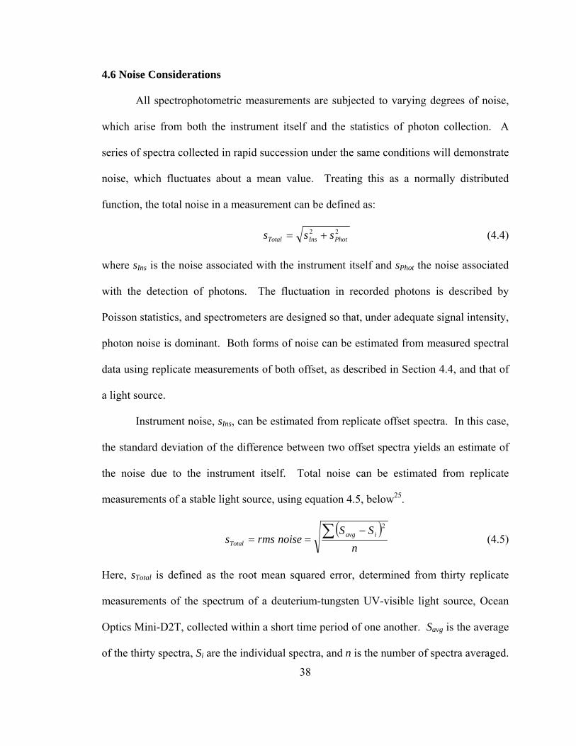
4.6 Noise Considerations

All spectrophotometric measurements are subjected to varying degrees of noise,

which arise from both the instrument itself and the statistics of photon collection. A

series of spectra collected in rapid succession under the same conditions will demonstrate

noise, which fluctuates about a mean value. Treating this as a normally distributed

function, the total noise in a measurement can be defined as:

22PhotInsTotal sss += (4.4)

where sIns is the noise associated with the instrument itself and sPhot the noise associated

with the detection of photons. The fluctuation in recorded photons is described by

Poisson statistics, and spectrometers are designed so that, under adequate signal intensity,

photon noise is dominant. Both forms of noise can be estimated from measured spectral

data using replicate measurements of both offset, as described in Section 4.4, and that of

a light source.

Instrument noise, sIns, can be estimated from replicate offset spectra. In this case,

the standard deviation of the difference between two offset spectra yields an estimate of

the noise due to the instrument itself. Total noise can be estimated from replicate

measurements of a stable light source, using equation 4.5, below25.

( )

nSS

noisermss iavgTotal

∑ −==

2

(4.5)

Here, sTotal is defined as the root mean squared error, determined from thirty replicate

measurements of the spectrum of a deuterium-tungsten UV-visible light source, Ocean

Optics Mini-D2T, collected within a short time period of one another. Savg is the average

of the thirty spectra, Si are the individual spectra, and n is the number of spectra averaged.

38

All spectra have been corrected for dark current, and were collected at 100 ms integration

time. From these measurements and equation 4.5, the total noise was determined to be

178 counts at 75% saturation. Figure 4.5 shows the root mean square error spectra of the

B&W-TEK spectrometer used in this research.

Figure 4.5: Root mean squared error of the B&W-TEK spectrometer used in this research. The total

noise was calculated as the root mean squared error of thirty spectra of an Ocean Optics deuterium-

tungsten light source, Mini-D2T.

39

40

For the B&W-TEK spectrometer used in this research, sTotal was calculated as 178 counts.

The total noise value calculated here is only valid if sufficient photons are collected, thus

ensuring that photon noise is the dominant source of noise. To ensure this criterion is

met, recorded intensities are typically maintained at ~75% of the saturation value of the

pixels (~65,000 counts for B&W-TEK BTU142), although this cannot always be

achieved across the entire wavelength region of a spectrometer.

CHAPTER 5: SPECTRAL ANALYSIS

5.1 Introduction: Principles of Differential Optical Absorption Spectroscopy

Differential Optical Absorption Spectroscopy, or DOAS, is a spectroscopic

technique used to determine the concentration of atmospheric constituents by application

of the Beer-Lambert Law:

(5.1) lceII )(0 )()( λσλλ −=

where I(λ) is the transmitted intensity of light at wavelength λ with initial intensity I0(λ),

after transmission along pathlength l in centimeters, containing concentration c in units of

molecules per cm3 of a constituent with absorption cross-section σ with units cm2 per

molecule 26. From equation 5.1, the optical density, OD(λ), can be defined as:

( ) lcIIOD )()()(ln)( 0 λσλλλ −== (5.2)

and the concentration of the constituent can be determined using the relationship:

))(/()( lODc λσλ −= . (5.3)

equations 5.1-5.3 are applicable in most laboratory settings, but in the open atmosphere

using light path-lengths of several kilometers, the Beer-Lambert Law must be modified to

include extinction from elastic Rayleigh and Mie scattering processes27. Here, extinction

refers to the loss of light from a direct beam, and can be thought of as both scattering and

absorption. Rayleigh scattering, the elastic scattering of light by air molecules, is treated

as an additional extinction process with extinction cross-section σR(λ).

41

The overall extinction due to Rayleigh scattering, )(λε R , can be defined as a

function of wavelength and the concentration of scattering species using the

expression

scatterc

28,29:

scatterRR c)()( λσλε = . (5.4)

In like manner, elastic scattering by aerosols (Mie) is also treated as an extinction process

with wavelength dependent extinction cross-section )(λσ M , and overall extinction 27:

nMM

−= λσλε )( (5.5)

where n is an integer between 1 and 4 26. Thus, equation 5.1 can be re-written to include

the extinction due to Rayleigh and Mie scattering. Additional absorbing species are also

included by summing over all species j:

. (5.6) ⎥⎦

⎤⎢⎣

⎡++−= ∑ )()()()()( 0 λελελσλλ MRj

jj cleII

The processes outlined above describe absolute extinction using the Beer-Lambert

Law, in which the features of a spectrum are described as the attenuation of source

intensity . Spectroscopic analysis in the atmosphere, however, often requires the use of

differential as opposed to absolute extinction. As most atmospheric absorbers and

scatterers are present or assumed to be present in the air mass probed, it is difficult to

obtain reference intensity I

0I

0(λ) containing no spectral signature of the jth absorbing

species or extinction due to Rayleigh and Mie scattering. Differential optical absorption

spectroscopy overcomes this limitation by modification of the reference intensity, and

isolating those spectral features which differ from that estimation. To illustrate this,

consider the spectrum of Figure 5.1.

42

Figure 5.1: An absorption band shown as a departure from the true I0(λ) as in laboratory

spectroscopy and as a departure from I’0(λ), as in differential spectroscopy.

Here, two absorption bands are defined as the difference in intensity between points

where the spectrum is relatively smooth (λ1 and λ3), and points where the spectrum has

changed rapidly in intensity (λ2 and λ4), as opposed to departures from true intensity ,

as is the case for laboratory extinction measurements. If those points on the smooth

portion of the spectrum are extrapolated, they will describe a smooth, broad-band

0I

43

function absent of narrow-band features, given in Figure 5.1 as )('0 λI . This implies that

a separation is possible, isolating the broad-band, smooth features of the spectrum from

narrow-band features. If the extrapolated smooth portion is subtracted from the overall

spectrum, the narrow-band, or differential features can be isolated. As the extinctions

due to Rayleigh and Mie scattering, given by equations 5.4 and 5.5, are broad-band

features with respect to wavelength, the differential, narrow-band structure of the

measured spectrum is considered to represent only absorption features. However, such a

separation also removes those absorptions or broad-bandwidth absorption features. If the

DOAS technique is to be quantitative, a means of isolating the narrow-band, differential

features from the absorption cross-sections σ of those species present at the time of

collection must also be used 26,27,30-33.

By analogy to the extrapolation and removal of the broad-band component of a

measured spectrum shown in Figure 5.1, the absorption cross-section of the jth species

can also be separated into narrow-band and broad-band components. Thus, each cross-

section is expressed as the sum:

bandnarrowjbandbroadjj )())( λσλσλσ += (5.7)

Using the broad-band component of equation 5.7, the reference intensity I’0(λ), in the

absence of differential absorption, previously defined as the extrapolation of the smooth

points of the measured intensity spectrum, can be mathematically defined as:

(5.8) ⎥⎦

⎤⎢⎣

⎡++−= ∑ )()())(exp)()(' 00 λελελσλλ MRjbandnarrow

jj clII

44

Accordingly, the intensity I(λ) can be described using the narrow-band component of the

absorption cross-section of the jth species. Lastly, following the Beer-Lambert Law, the

differential optical depth, DOD(λ), can be defined as:

∑−==j

jbandnarrowj clIIDOD )())(/)('ln()( 0 λσλλλ (5.9)

In practice, the extrapolation of the broad-band components, and separation of the

narrow-band components of both atmospheric intensity and absorption cross-section

spectra is accomplished by robust mathematical techniques, the details of which are given

in sections 5.6 and 5.7 of this chapter.

To determine the concentration of the jth species, the differential absorption cross-

section σi(λ)rapid is fitted by least squares regression to the measured differential optical

depth, as described in section 5.8 of this chapter. The resultant fit coefficient is the

concentration of the jth species, or in the case of an unknown pathlength, the differential

slant column density of the jth species1,27. The least squares fitting procedure often

includes a correction for wavelength calibration differences between the measured

differential optical depth spectrum and the reference differential absorption cross-

sections, as well as corrections for stray light in the measurement spectrometer.

Additional corrections for instrumental spectral broadening and noise are also made prior

to the least squares fit. Each step of the differential spectral analysis presented above and

the fundamental scientific basis for each process is detailed in this chapter. The

rudimentary steps of this analysis, and the relevant sections of this chapter in which each

processes is described, are shown in Figure 5.2.

45

Figure 5.2: Pre-processing of both collected atmospheric intensities (left) and reference absorption

cross-sections (right), shown with references to relevant sections of this document. The necessary

output for subsequent analysis procedures are the design matrix A, data matrix B, the wavelength

pixel mapping function for the j species to be analyzed, as well as the convolved reference absorption

cross-sections with their original wavelength grids.

Note that no distinction has been made at this point between continuous and measured,

discrete spectra. The concept of discrete spectra is introduced later, and was purposely

omitted from the above description of differential absorption, which is a description of

the physical nature of light absorption. In points of discussion where this distinction is

made, discrete data points will be indicated by the subscript i and the subscript iHR,

indicating the wavelength grid of the DOAS spectrophotometer and the higher resolution

wavelength grids of reference absorption cross-sections, respectively.

46

47

5.2 Species Measurable by Differential Techniques

DOAS techniques for the UV-visible region are concerned with molecules that

absorb light in the 310 to 770 nm wavelength region. Electromagnetic radiation below

310 nm is strongly attenuated by the Hartley band of ozone, and wavelengths below 180

nm are almost completely absorbed by atmospheric oxygen34,35. Differential

spectroscopy is also possible for longer wavelengths, but is limited by the strong

absorptions of H2O and CO2 in the infrared. In practice, the nature of the excitation light

source also limits wavelength coverage, and therefore the number of species capable of

being analyzed.

The Max-Plank Institute maintains a database of atmospheric species which

absorb light within the UV-visible wavelength region, and currently contains

approximately 670 species36. This is a significant reduction in the number of species to

be considered in light of the vast number of gaseous species present in the atmosphere at

any given time. Despite the large number of atmospheric species capable of absorbing

UV-visible light, the majority of atmospheric species are unsuitable for differential

spectroscopic applications. Even if the species is a strong absorber, or is present in high

concentrations, that species cannot be detected using differential techniques if it lacks

sufficient narrow-band absorption features, or structure, in its absorption cross-section

spectrum, as described in section 5.126,32,33. For example, Figure 5.3 shows the absolute

absorption cross-section of nitric acid. Despite a relatively large absolute absorption

cross-section, nitric acid lacks the narrow, structured absorption features necessary for

differential spectral analysis.

Figure 5.3: Absolute absorption cross-section of nitric acid. The lack of peaked structure necessary

for differential analysis is clearly evident.

That is, if the extrapolation and differentiation of Figure 5.1 is applied to the cross-

section of nitric acid, the resultant spectrum would be a monotonous function that would

not impart distinct narrow-band features to an absorption spectrum. The vast majority of

absorbers of ultra-violet or visible radiation present in the atmosphere demonstrate

absorption spectra similar to that of nitric acid, having little or no narrow-band absorption

features, which can alternatively be thought of as multiple peaks and valleys in the

absorption cross-section. In contrast, Figure 5.4 shows the absolute and differential

absorption cross-sections of NO2. Note the broad-band component of the absorption 48

cross-section, calculated here as a moving average smoothed version of the original

spectrum.

Figure 5.4: Absolute and differential absorption of NO2. Two strong differential features are

indicated by the arrows.

The broad-band component represents not only the overall trend in the absorption, but

also the shape of the excitation light source and any broad-band instrument effects, for

example, poor transmission of certain wavelengths in the optical components. Arrows

indicate examples of the narrow-band structure necessary for differential spectral

analysis.

Of the approximately 670 documented gaseous species that absorb UV-visible

radiation in the atmosphere, only a small percentage of those species have absorption 49

50

spectra with the characteristic narrow-band structure necessary for differential spectral

analysis. At the time of writing, approximately 20 gaseous species capable of being

detected and analyzed by UV-visible differential absorption spectroscopy, using either

natural or artificial light sources, have been identified27. Figure 5.5 shows the absorption

cross-sections of 10 atmospherically relevant species which have been detected and/or

quantified using differential optical absorption spectroscopy. Note the narrow-band

absorption features of each spectrum in contrast to the relatively smooth nature of nitric

acid shown in Figure 5.3

Figure 5.5: Differential absorption cross-sections of 10 species commonly found in DOAS analysis.

The spectra were taken from: NO37, NO238, HONO39, SO2

40, HCHO41, Benzene42, ClO43, BrO44, O345,

and O446

5.3 Analysis Window Selection

As important as the selection of species to be included in the differential analysis

is the narrowing of available wavelengths to smaller wavelength regions, or, as

commonly presented in the literature, the selection of analysis windows where species of

interest absorb strongly. Equation 5.9, defining differential absorption, could

51

52

theoretically be applied across the entire UV-visible wavelength region, limited only by

the spectral coverage of the DOAS instrument. In practice, however, only limited regions

of the entire spectral region of the instrument are used for differential analysis30,31.

Although there is no single rule dictating the selection of the spectral windows for

analysis, there are three important guidelines. First, the spectral window chosen must

contain significant differential absorption structure of the species of interest. Illustrations

such as Figure 5.5, which show the differential absorption features of a great many

species detectable by differential methods, are a valuable tool in wavelength region

selection. Secondly, wavelength regions should be selected where there is minimal

interference from other species also demonstrating differential absorption. Ideally, a

wavelength region where only the species of interest absorbs would be selected, although

this situation is rarely encountered. As an example, consider the absorption of NO2,

which covers a large portion of the UV-visible wavelength region. Based on Figure 5.5,

it would be prudent to analyze atmospheric spectra for NO2 above approximately 400 nm,

based on the lack of absorption structure of other species at these higher wavelengths,

although consideration to the capabilities of the particular spectrometer used must be

given. Above 400 nm, it is apparent that NO2 has strong differential features, with only

minor interference from the O4 collisional complex. Although extinction due to

absorption scales with both the magnitude of the absorption cross-section and

concentration, analysis window selection is primarily based on the presence of absorption

features. The most appropriate choice for an NO2 fitting window would therefore be

selected above 400 nm. It should also be noted that even if a species is not a target

analyte but absorbs differentially in a selected wavelength interval, that species must be

53

included in the analysis by equation 5.9, even if that species is not anticipated to be

present at concentrations above the detection limit of the instrument.

Lastly, the spectra of the excitation light source must be considered. In many

cases, the emission spectrum of the light source will exhibit significant structure, which

may interfere with differential analysis. If sun or moonlight is used as a source, much

care must be taken to avoid regions where strong solar Fraunhoffer (native emission lines

in the solar spectrum) lines occur1. Removal of these spectral features can be difficult

even when a reference solar spectrum is subtracted from the measured data, due to the

broadening of solar lines from molecular rotational Raman scattering, also known as the

Ring effect47,48.

The selection of wavelength windows for differential analysis is greatly simplified

by the amount of research conducted using the differential technique over more than

three decades. For the majority of species shown in Figure 5.5, as well as several others,

standard wavelength windows, or intervals, for their analysis have been established in the

literature, following the guidelines detailed above. Only for a newly discovered species

exhibiting differential absorption features, an infrequent occurrence, would a rigorous

analysis to determine the most appropriate analysis window be necessary, although some

consideration to the individual instrument and atmospheric conditions during the time of

collection must be given. Table 5.1 summarizes the analysis windows used for ten of the

most common species quantifiable by differential optical absorption spectroscopy. From

Table 5.1, it can be seen that the majority of the species shown can be quantified within

several spectral windows. Note the difference in windows between techniques using

artificial and solar light. These differences can be attributed to the avoidance of spectral

54

features associated with the Fraunhoffer lines found in the solar spectrum. Note that

artificial light sources are capable of projecting wavelengths of radiation which do not

reach the surface of the Earth from natural sunlight.

SPECIES LIGHT SOURCE / INTERVAL(nm) REFERENCE

Benzene Artificial, 250-290 49

BrO Solar, 346-359 50

ClO Artificial, 284-302 51

Formaldehyde (HCHO) Artificial, 323-335

Solar, 335-357

30,52,53

HONO Artificial, 350-375 33

NO2 Artificial, 323-335

Artificial, 345-380

Solar, 430-455

Artificial, 400-450

Solar, 430-441

1,30,32,54-56

NO3 Lunar, 656-668

Lunar, 646-682

Solar, 640-680

57-59

O3 Artificial, 325-350

Solar, 400-453

Solar, 315-330

31,32,60-62

O4 Solar, 347-388, 415-682

Solar, 335-367

Solar, 460-490

7,63,64

SO2 Solar, 303-313

Solar, 307-316

Solar, 316-325

5,65,66

Table 5.1: Wavelength windows of common analytes used in past differential optical absorption

studies.

55

5.4 Processing of Absorption Cross-Section Spectra Prior to Differential Analysis

Analysis of measured differential optical absorption spectra to determine the

concentration of gaseous species relies on the availability of high-quality absorption

cross-section spectra (σ(λiHR), equation 5.1 for discrete case), which can be processed and

subsequently fitted by least squares techniques to the measured optical depth spectra. To

this end, absorption cross-sections can be measured in the laboratory using the DOAS

instrument, a suitable light source, and a gas handling system to deliver species of interest

into an optical cell32. The advantage of this method of acquiring reference absorption

cross-sections is that the collected spectra will include all spectral artifacts introduced by

the instrumentation, as well as a consistent wavelength calibration and resolution as

collected atmospheric spectra. However, laboratory collection of high-quality absorption

cross-section data requires a gas handling system, standardized trace gases, and

temperature control capabilities. At the lower resolution of a typical DOAS

spectrometer, these spectra will typically be of use only for that particular instrument.

As an alternative to laboratory measured trace gas absorption spectra, it is

commonplace within the DOAS scientific community to use absorption spectra published

from laboratories dedicated to the acquisition of temperature dependent, high-resolution

gaseous absorption spectra. The earliest measurements of NO3 and other trace species by

differential methods relied on absorption cross-section data collected in such a manner,

and that precedence continues in the most current DOAS literature58,64. In addition to

being of much higher quality than what is capable of a typical DOAS instrument (typical

resolution of ~1 nm), such spectra are readily available and maintained in electronic

databases, such as that of the Max-Plank Institute, Division of Atmospheric Chemistry.

56

In order to use absorption cross-sections collected from outside sources, a number of

preprocessing steps are necessary27. The disadvantages of using spectra from outside

sources, aside from the additional mathematical processing necessary, is the need for

intensive instrumental characterization to realize the effects of stray light and spectral

artifacts on measured spectra versus those collected from outside sources. The

mathematical techniques used in the preprocessing of absorption cross-section spectra are

detailed in Sections 5.4b-5.4d of this thesis. However, it is necessary first to examine the

scientific basis of these techniques, which are strongly rooted in principles of

spectroscopy, optics, and digital signal processing, and are detailed in section 5.4a,

below.

5.4a Recording of spectral data by spectrophotometers

Differential optical absorption spectroscopy is a spectrophotometric technique,

and as such, there are several common elements to all DOAS instruments. All DOAS

instruments require a suitable light source, such as the Sun, a high intensity UV-visible

lamp, or UV-visible laser. Suitable optics, capable of collecting light emitted by the

source and directing that light to the spectrophotometer, such as telescopes, focusing

lenses, and fiber optics are also necessary. Details of the instrument used in this work are

presented in Chapter 4. Once directed to the spectrophotometer, collected light is

focused onto an entrance slit, then to a wavelength selection component. The wavelength

selector, whether a prism, filter, or grating, separates the collected white light into its

component wavelengths and disperses these wavelengths onto a detector. The detector

registers the intensity of light at discrete wavelength intervals as an analog signal, which

is subsequently converted to a digital signal suitable for computer storage or readout.

57

This process has several implications on the information content as well as appearance of

the collected spectrum, and thus the mathematical treatment applied.

To illustrate the process of spectral collection and the attenuation of a given

spectrum by the collection and discretizaton of the spectral signal, consider a spectrum of

solar radiation prior to passing through the Earth’s atmosphere. The sun itself is

considered a spherical light source, located 1.5 x 108 kilometers from the Earth’s surface,

with a diameter of 1.4 x 106 kilometers. Un-attenuated by the Earth’s atmosphere, the

sun approximates a blackbody emitter with a temperature of approximately 5770 K,

emitting a continuum of electromagnetic radiation from approximately 200 to 3000 nm14.

This continuum passes through the Earth’s atmosphere and, ignoring absorption

processes for the purposes of demonstration, is assigned intensity I(λ), as in Figure 5.6a,

adapted from Stutz and Platt, 199667.

Figure 5.6: Attenuation of the solar spectrum during collection and pixelation by a

spectrophotometer.

Intensity I(λ) is gathered by the collection optics of the instrument and directed to the

entrance slit of the spectrophotometer. Changes to the shape of the intensity spectrum are

introduced by the collection optics and the limited resolution of the spectrometer itself,

giving altered continuous intensity spectrum I(λ)*, as in Figure 5.6b. How the instrument

58

alters the continuous spectrum can be described by function F, known as the response or

instrument function, and intensity I(λ)* given by 27,68:

(5.10) ∫+∞

∞−

−= ')'()'()*( λλλλλ dFII

Recording of the continuous, convolved spectrum I(λ)* by the detector, which maps

wavelength ranges to discrete pixels or bins, destroys the continuous nature of the

spectrum and degrades information content, yielding intensity spectrum I(pixel)*.

I(pixel)* can alternatively be expressed in terms of discrete wavelengths as I(λ(i))*, if

each pixel is assigned a wavelength by a calibration function, as detailed in section 5.9.

As I(λ(i))* represents an actual intensity spectrum collected by a DOAS

instrument, the model of attenuation in the atmosphere, previously defined for continuous

spectra by equation 5.6 above, can be modified to better express the discrete, instrument

function attenuated nature of the data as:

(5.11) ⎥⎦

⎤⎢⎣

⎡++−= ∑ )()()*)(*)()*( 0 iMiRji

jjii cleII λελελσλλ

where *)( ij λσ is the absorption cross-section of the jth species, which has been subjected

to instrument function convolution (*) and discretization to the wavelength grid of the

DOAS spectrophotometer )( iλ . Following the differential absorption methods detailed

in section 5.1, optical depth, previously defined by equation 5.2, can be expressed for the

discrete, convolved case for j trace gas species as:

( ) ∑−==j

jijiii clIIOD *)(*)(*)(ln)( 0 λσλλλ . (5.12)

59

In like manner, the differential optical depth, previously defined for the continuous case

by equation 5.9, can be expressed for actual data as:

∑−==j

jrapidijiii clIIDOD *)()*)(/*)('ln()( 0 λσλλλ . (5.13)

Equation 5.13 serves as the regression model for the spectral analysis employed in this

research, as it deals with discrete, instrument attenuated spectra as encountered in actual

analysis.

Manipulation and processing of absorption cross-section spectra attempts to

replicate, as closely as possible, the attenuation of spectra as they are collected and

recorded by a spectrophotometer. In a DOAS framework, the goal is to apply the above

principles to absorption cross-sections collected with a spectrophotometer different than

that of the DOAS instrument, so that the resultant spectra are as if they were collected

with the DOAS spectrophotometer itself. The mathematical routines used to replicate the

effects of the instrument function as well as discretization to the pixels of the DOAS

spectrophotometer are detailed in sections 5.4b and 5.4c, respectively.

5.4b Convolution with the instrument function

The instrument function of a spectrophotometer describes the attenuation of light

by diffraction and optical elements that occurs during the collection and dispersion of

electromagnetic radiation. These effects can be both broad-band, introduced, for

example, by poor transmission of certain wavelengths in the optical setup, or narrow-

band, such as the effects introduced by diffraction, and stray light impinging on certain

regions of the detector 69. As the DOAS technique is primarily concerned with narrow-

band phenomena over limited wavelength ranges, broad-band instrumental effects are

60

largely removed as the slowly varying component of measured and reference spectra, as

described in Section 5.1. However, the narrow-band effects of spectral sampling must be

accounted for if using absorption cross-sections collected with spectrophotometers other

than that of the DOAS instrument. Narrow-band effects can be attributed to both the

diffraction efficiency of the wavelength separation device and the optical setup of the

spectrometer which determines the resolution of the instrument, as well as to artifacts

introduced to measured spectra, from, for example, faulty detector pixels. Spectral

artifacts can be detected and removed through instrument characterization, and are not

typically considered to be part of the instrument function. Henceforth, the term

instrument function will refer to those processes that control the resolution of the

instrument, unless explicitly stated otherwise. In general, the instrument function can be

determined by measuring the spectrum of several emission lines with known line widths.

For the case of the spectrophotometer used in this research, the instrument function is a

Gaussian function with full width at half maximum of 0.282 nm, as described in Chapter

4. In Figure 5.6 above, the alteration of the spectrum from trace a to b shows these

narrow-band effects, and can be thought of as a “smearing out” of the fine structure

present in the continuum spectrum.

Equation 5.10, describing the attenuation of the continuum intensity with the

instrument function F:

(5.10) ∫+∞

∞−

−= ')'()'()*( λλλλλ dFII

is not practical for DOAS applications, however, as continuum signals are not dealt with.

A more practical presentation of convolution is the generalized, discrete form, which can

61

be applied to any two signals. In this form, the equation is referred to as the convolution

sum, expressed as 70:

(5.14) ∑−

=

−=1

0)()()(

M

jjiFjhiy

where h is any signal of length M running from 0 to M-1, such as an absorption cross-

section, and F is any signal of length N running from 0 to N-1, such as the instrument

function of the DOAS instrument. M and N are indices representing, for example, a

spectrum running from λ1 to λ2. The resultant signal y, the convolution of the two

signals, is an N + M -1 point signal running from 0 to N + M -2. By the above equation,

each point of y at index i can be calculated individually70. For instrument or filter

functions F larger than 64 data points, convolution using equation 5.13 becomes

relatively slow. By the convolution theorem, convolution in the time domain, as in

equation 5.14, is equivalent to multiplication in the frequency domain. Thus, equation

5.14 can be expressed for the frequency domain as:

(5.15) ))](())(([)( 1 jiFjhiy −ℑ∗ℑℑ= −

where is the Fourier transform to the frequency domain and the inverse Fourier

transform to the time (wavelength) domain

ℑ 1−ℑ

68. By equation 5.15, absorption cross-section

spectra of trace gases can be convolved with the instrument function of the DOAS

instrument, smoothing the high resolution spectra as if it were collected with the DOAS

instrument itself. This convolution transforms )( iHRλσ to *)( iHRλσ , more representative

of a spectrum collected with the DOAS instrument. Again, instrument function in this

context refers only to those processes contributing to the resolution of the instrument.

62

63

Two important properties of the convolution theorem must be accounted for to

ensure a proper convolution. First, both the spectra and instrument function must have

the same number of elements prior to transformation to the frequency domain. Secondly,

the convolution theorem treats signals as if they were periodic, which can produce

wraparound issues if not dealt with properly. The first issue is easily dealt with by

padding the signals with zeroes to achieve the same number of elements. The second

issue is also dealt with by padding both signals with zeroes to length M + N-1, where M

and N are the original signal lengths for the spectrum and instrument function.

An example of this convolution is shown in Figure 5.7, using the NO2 absorption

cross-section of Figure 5.4.

Figure 5.7: Convolution of the absorption cross-section of NO2 by the instrument function of a DOAS

spectrophotometer. In this case, the convolution was implemented by multiplication in the

frequency domain.

The graphs shown in Figure 5.7 were obtained following the convolution routine as

detailed by Press and adapted for implementation in Mathcad71. For practical purposes,

however, the time consuming process of convolution as described above has been

incorporated into most software written for the purpose of DOAS spectral analysis, for

example the WinDOAS and SCIATRAN software implemented in this research 72,73. 64

Note that although spectra collected from outside sources contain the instrument

function of the original instrumentation, the resolution of those instruments are typically

much finer than that of a DOAS spectrophotometer, and as such can be ignored 27. This

is demonstrated in Figure 5.8, showing the broadening of a spectral line by a high and

low resolution spectrophotometer, as well as the broadening of a spectral line collected

by a high resolution instrument (0.2 nm) and subsequent convolution by the instrument

function of an Ocean Optics spectrometer (PC2000) used for parts of this research (0.8

nm).

Figure 5.8: Convolution of a spectral line with low and high resolution Gaussian instrument

functions. In trace a, a spectral line is convolved with the instrument function of the DOAS

instrument, with full-width at half maximum 0.8 nm. b shows the convolution of the same spectral

line with a theoretical instrument function of full-width at half maximum 0.2 nm. c demonstrates the

convolution of the product in b with the lower resolution instrument function of a. It can be seen that

the product of c is identical to the product of a. Thus, the instrument function of the high resolution

spectrum does not need to be removed prior to convolution.

65

66

Again, this method is useful for degrading the resolution of narrow-band spectral

features, but does not correct for any slowly varying, broad-band instrumental features

(non-resolution component). Removal of those features is accomplished by high pass

filtering of the absorption cross-sections, Section 5.7.

5.4c Spline to grid of spectrometer

The final step in the recording of a spectrum by a DOAS spectrophotometer as

detailed in Section 5.4a above is the discretization of the continuous spectrum to the

individual pixels of the detector. In the case of high resolution cross-section spectra

obtained from outside sources, which have previously been pixilated to the detector of the

spectrophotometer with which they were collected, this can be thought of as re-mapping

the spectrum to the pixels of the DOAS detector. As the high resolution absorption cross-

sections have much finer wavelength spacing and different wavelength-pixel mapping

functions than that of a typical DOAS instrument, it is often not possible to find matching

wavelength points. Therefore, it is desirable to use a mathematical routine to interpolate

the high resolution spectra to the wavelength grid of the DOAS instrument, imitating the

discretization of the spectrum as described in section 5.4a. The most common approach

to the interpolation problem in DOAS analysis is to implement the cubic spline. This

method provides a relatively fast means of estimating the value of a point using values

surrounding it, and is relatively robust against nonlinearities in the detector’s wavelength

pixel mapping67. A rigorous investigation of interpolation errors in the framework of

differential spectroscopy was conducted in 1996 by Roscoe, Fish and Jones, which

determined that the cubic spline was superior over both linear and quadratic interpolation

methods over a large range of theoretical spectrophotometer resolutions and wavelength

pixel mapping nonlinearities74.

Interpolating reference absorption cross-sections to the wavelength grid of a

DOAS spectrophotometer, as mentioned previously, is a necessary step in the spectral

analysis process if the references are to be fitted by least squares methods to differential

optical depth spectra74. By this process, the discretization of a continuous or in the case

of high-resolution spectra, relatively continuous, spectra can be accomplished. Using the

instrument function convolved cross-section of NO2 from Figure 5.7, the process of

interpolation by cubic splines can be demonstrated.

Figure 5.9: Results of a cubic spline interpolation of the high resolution NO2 absorption cross-section

to the wavelength grid of a lower resolution DOAS spectrometer. Traces a and b show the original

spectrum plotted as discrete data points and as a continuous spectrum, respectively. Traces c and d

show the spectrum after a cubic spline interpolation to the relatively rough grid of the DOAS

instrument, as discrete data points and as a continuous spectrum, respectively. The reduction in

information content between traces a and c is clearly visible.

67

68

Figure 5.9 demonstrates the application of cubic spline interpolation from the fine grid of

the original spectrum to the relatively “rough” grid of a DOAS spectrophotometer. Over

an arbitrary wavelength region of 415.00 to 416.00 nm, the convolved, high resolution

reference spectrum of Voigt38 has N = 101 data points, evenly spaced at 0.01 nm

intervals. Over the same wavelength region, the detector of an Ocean Optics USB2000

spectrometer used in this research has N = 12 data points, evenly spaced at 0.1 nm

intervals from 414.93 to 416.03 nm. In this case, an operator could theoretically select

manually those data points from the high-resolution spectrum of NO2. However, this is

not done for the purposes of demonstrating the cubic spline interpolation. Cubic spline

interpolation techniques are more representative of the actual process of sampling

discrete points from a continuous spectrum that occurs when a spectrophotometer records

data. Based on Figure 5.9, it can be shown that despite the ~6 fold reduction in

information content, the interpolated spectrum strongly resembles the original. The

mathematical details of the cubic spline interpolation used to produce the above spectra

are given below.

Given a function, or in this case a spectrum, f(x) at known points x1, x2, …, xN

without an analytical expression of f(x) that allows the calculation of values at arbitrary

points, it is still possible to estimate the value at an arbitrary point by means of an

interpolation scheme. A very simple scheme, for example, would be to draw a smooth

curve through the known points of f(x) and estimate arbitrary values from that curve. In

the framework of spectral analysis, however, a more exacting, mathematical means of

estimating data points, in this case the points are the wavelength bins of the DOAS

detector, is desired. For this, as mentioned above, the cubic spline interpolation scheme

is used. Using the arbitrary function )( ii xyy = , for Ni ...1= , and focusing on the interval

xj to xj+1, linear interpolation in that interval can be given as:

1++= jj ByAyy (5.16)

where

jj

j

xxxx

A−

−=

+

+

1

1 jj

j

xxxx

AB−

−=−=

+1

1 . (5.17)

Equation 5.16 is a linear equation with zero second derivative within each interval and an

infinite second derivative at each abscissa xj. The cubic spline is based on finding an

interpolation formula that has a smooth first derivative and continuous second derivative

both within a given interval and at its boundaries 71. To fulfill both conditions, a cubic

polynomial can be added to the right hand side of each interval within equation 5.16,

whose second derivative varies linearly from to and has zero values at x"jy "

1+jy j and xj+1.

To accomplish this, equation 5.16 can be re-written as:

(5.18) "1

"1 ++ +++= jjjj DyCyByAyy

where

21

3 ))((61

jj xxAAC −−= + 21

3 ))((61

jj xxBBD −−= + (5.19)

An additional caveat of the cubic spline is that the first derivative of y must be

continuous across the boundary between two intervals. Requiring this continuity and

using it to derive equations for the first and second derivatives of y is the main aspect of

the cubic spline. The first derivative of equation 5.18 can be written as:

"11

2"

1

2

1

1 )(6

13)(6

13+++

+

+ −−

+−−

−−

−= jjjjjj

jj

jj yxxByxxAxxyy

dxdy (5.20)

69

In order to impart continuity to the first derivative across interval boundaries, equation

5.20 is evaluated for x = xj across interval xj-1 to xj and set to be equal to the same

equation evaluated for the interval xj to xj+1. This new equation can be written for the

interval j = (2, …, N-1), with rearrangement, as:

1

1

1

1"1

1"11"1

1

636 −

−

+

++

+−+−

−

−

−−

−

−=

−+

−+

−

jj

jj

jj

jjj

jjj

jjj

jj

xxyy

xxyy

yxx

yxx

yxx

(5.21)

Equation 5.21 represents N-2 linear equations with N unknowns y”. To obtain a unique

solution, two further boundary conditions must be specified, and are typically applied at

x1 and xN. The most common way of applying boundary conditions is to set one or both

of and equal to zero, and is frequently referred to as the “natural” cubic spline 1"y Ny"

71. Additional boundary conditions can be applied in the interpolation process, and in

most high quality calculation software packages several options are available to the user.

For practical purposes, however, the “natural” cubic spline yields satisfactory results with

minimal computational effort.

5.4d Absorption cross-section processing in practice

To this point, the processing of absorption cross-section spectra to make them

suitable for inclusion in the differential optical depth least squares fitting procedure has

been detailed from the standpoint of replicating the physical processes that occur during

the collection of a spectrum by a DOAS spectrophotometer. These processes include

convolution with the resolution component of the instrument function to replicate the

limited resolution of the DOAS spectrophotometer and cubic spline interpolation to

replicate the discretization that occurs when the detector bins a spectrum that is

continuous in wavelength to the pixels of the detector. At this point, it is beneficial to

70

71

compare an absorption cross-section collected with the DOAS spectrophotometer to that

of a high-resolution spectrum from a secondary source that has been processed by the

mathematical routines described in Sections 5.4b and 5.4c. An additional step, the least

squares regression and removal of a 4th order polynomial, representative of the broad-

band instrument function, has been performed for both the measured and processed

spectra. This additional step is detailed further in Section 5.7. For the sake of

completeness, the example NO2 spectrum used in previous examples will be used, and

compared to an absorption cross-section of NO2 collected with the Ocean Optics

USB2000 spectrophotometer used for parts of this research.

Figure 5.10: Differential absorption cross-section of NO2 collected by a low-resolution DOAS

spectrometer (blue trace) and a spectrum processed from a high resolution spectrum after

convolution and cubic spline interpolation (red trace). For comparison, a 4th order polynomial,

representing the broad-band instrument function of each instrument, has been removed from both

spectra. The slight differences can be attributed to variations in calibration between the two

instruments, and can be corrected in the fitting process.

The data shown in Figure 5.10 are quite remarkable, as it demonstrates several

important aspects of the processing of spectral data prior to least squares analysis to

derive concentration. Firstly, the effectiveness of the instrument function convolution is

apparent by comparison of the peak widths between the two spectra. Although not

represented for the purposes of visualization, the red trace was interpolated to the

wavelength grid of the DOAS spectrophotometer, a reduction in data from 11,000 values

to 1080. The above also demonstrates the effectiveness of the regression and removal of

slowly varying functions, in this case a 4th order polynomial, as representative of the

slowly varying component of the absorption cross-section (equation 5.7) as well as any

72

73

broad-band features introduced through instrumentation. The removal of broad-band

features from spectral data is discussed in further detail in Sections 5.6 and 5.7 of this

chapter. Additionally, Figure 5.10 highlights an important source of error in differential

analysis, that is, the slight wavelength misalignment between the reference absorption

cross-sections and the DOAS instrument. To correct this misalignment, an adjustment of

the wavelength calibration of each reference spectrum is included in the least squares

analysis procedure 67,75,76. This correction is detailed in Section 5.9.

5.5 Determination of Optical Depth

The primary data that is analyzed in differential optical absorption spectroscopy

are collected intensity spectra. As the technique is based on the absorption of light by

trace gas species, the analysis is based on the Beer-Lambert Law, equation 5.1. For each

intensity spectrum to be analyzed, a Fraunhoffer reference spectrum must be selected,

which is used to remove spectral lines associated with solar radiation. Reference

intensities are chosen such that a minimum amount of absorption features are present.

Following equation 5.12, the natural logarithm of the ratio of the reference intensity and

spectrum of interest is calculated. The resultant spectrum is known as the optical depth.

This division is usually sufficient to remove those spectral features associated with the

light source and isolate those features associated with extinction processes, such as

scattering and absorption. In a laboratory setting, where scattering is assumed to be

negligible, the resultant spectrum would contain only those features associated with

absorption. Figure 5.11 shows an optical depth spectrum calculated from scattered solar

radiation spectra collected on August 14, 2007 using equation 5.12.

Figure 5.11: Optical depth spectrum, collected on August 14, 2007. The spectrum shown here

represents the natural log of I0 and I, a Fraunhoffer reference spectrum and off axis spectrum,

respectively, shown in the inset, according to the Beer-Lambert Law. The strong overall slant of the

optical depth spectrum is the result of Rayleigh and Mie scattering, as well as the slowly varying

components of atmospheric absorbers. It is this slowly varying trend that must be separated prior to

least squares analysis to determine concentrations or slant column densities.

For spectra collected in the open atmosphere, the optical depth spectrum contains not

only narrow-band absorption features but those features associated with scattering and

broad-band extinctions, as in equation 5.11, above. These features are clearly visible in

Figure 5.11 as the overall slant or trend in the optical depth. The removal of these broad-

band features is a critical aspect of the DOAS technique, and is discussed in Section 5.6,

below.

74

75

5.6 Determination of Differential Optical Depth

In most DOAS applications, the broad-band features associated with Rayleigh and

Mie scattering, as well as absorption, are removed prior to least squares fitting, or

included in the fit routine as is the case for this research. In either case, these features are

treated as smooth functions26,27,30,31,77. On the surface, the assignment of scattering

features to an all-encompassing function seems arbitrary, but is strongly rooted in the

physics of light scattering. By equations 5.4 and 5.5, describing the extinction of light by

air molecules and particulate matter, respectively, simple representations of scattering can

be calculated. It is fortunate that extinction by air molecules and aerosols can be well-

approximated by simple power functions, as a full treatment of scattering in the

atmosphere would be computationally costly27. A more advanced treatment of

atmospheric scattering, necessary for the modeling of solar radiation in the atmosphere, is

given elsewhere in this thesis (Chapter 2), as it is not fully relevant to the discussion of

differential spectral analysis excepting the slowly varying behavior with wavelength. It

was previously demonstrated in sections 5.1 and 5.2 of this chapter that atmospheric

intensity spectra and the absorption cross-section spectra of trace gases have a broad-

band and narrow-band component, which can be separated using equation 5.7. As the

broad-band component of the cross-section is un-quantifiable in the presence of Rayleigh

and Mie scattering, the DOAS application is concerned only with the narrow-band

component, as in Figure 5.1. Therefore, the spectral analysis task is to isolate these

features and remove the un-quantifiable content, that is, scattering and broad-band

absorption. As in section 5.1, this can be thought of as the extrapolation and subtraction

of those points of a spectrum which do not change rapidly with wavelength. To

76

accomplish this, a slowly varying broad-band function must be removed from the

measured optical depth spectrum as well as the reference absorption cross-sections to be

included in the least squares fit to determine slant column densities or concentrations,

depending on the experimental setup. It should be noted that while the removal of the

broad-band trend in both the optical depth and absorption cross-section spectra prior to

concentration determination is mathematically sound by equations 5.7, 5.8, and 5.9, the

usual practice is to include the slowly varying component as an additional fit parameter,

as is the case in this research 73. This method can be thought of as the superposition of

the narrow-band components of the absorption cross-sections onto a broad-band trend.

The former method, however, makes for a more effective demonstration of differential

absorption.

Figure 5.12 illustrates the use of several broad-band functions to determine the

differential optical depth for the spectrum of Figure 5.11, above.

Figure 5.12: Broad-band component of an optical depth spectrum, determined by three methods.

The top row of traces show the slowly varying component of the optical depth spectrum, determined

by least squares regression of a 4th order polynomial, a moving average smoothed optical depth

spectrum, and a Bartlett (triangular) windowing smooth. Below each function is the differential

optical depth, calculated as the difference between the optical depth and the respective slowly

varying function. Although minor differences are present in each of the three differential absorption

spectra, these are largely confined to the end regions.

The regression of these broad-band functions serves as the extrapolation of the smooth

component of a spectrum, as demonstrated in Figure 5.1. From Figure 5.12, the choice of

function for the determination of differential optical depth, representing the extinction

due to Rayleigh and Mie scattering in the atmosphere, has only a relatively minor impact

on the final spectrum. It should also be noted that the DOAS technique is concerned only

with absorptions that are differential to a consistent function that is slowly varying with

respect to the absorption features present. Thus, the broad-band function could also be

represented as, for example, a sine or square wave, as long as the same function is 77

78

applied over the same wavelength region for each spectrum included in the model and the

spacing between the peaks is greater than that of the absorption cross-sections in the

model, although such a method would invariably introduce structure, and thus error, into

the regression, in addition to being a non-physical representation of broad-band features.

In the available software routines for DOAS analysis, the polynomial regression method

is typically used, and as such is commonplace in the literature73. Experience has also

shown that the polynomial method is more easily implemented and performs faster than

other methods of high pass filtering within various differential absorption fit routines, and

is the method implemented in this research.

5.7 Determination of Differential Absorption Cross-sections

Analogous to the determination of differential optical depth from measured

atmospheric intensity spectrum, the absolute absorption cross-sections to be used in the

determination of concentration or slant column density must be processed to remove

those features that are slowly varying with respect to wavelength, to conform to the

restrictions of equation 5.13. Broad-band features in absolute absorption cross-sections,

collected under laboratory conditions in which Rayleigh and Mie scattering are minimal,

are attributed to the general shape of the excitation source, the broad-band component of

the instrument function, and the natural shape of the absorption spectrum itself 27. Figure

5.4 shows the determination of the differential absorption cross-section of NO2, as

determined by a moving average smooth of the original spectrum. In practice, however,

absolute absorption cross-sections are truncated in wavelength to match that of the DOAS

spectrophotometer, and possibly further truncated to isolate wavelength regions where

interference from the light source and other absorbing species is minimal, as discussed in

section 5.3.26,27,32. Figure 5.13 below shows the differential absorption cross-section

calculation for NO2, that is, wavelength truncation, followed by the fit and removal of a

4th order polynomial. The wavelength interval chosen here, 350 to 460 nm, encompasses

several fitting windows used in previous DOAS research, as shown in Table 5.1.

Figure 5.13: The differential absorption cross-section of NO2. A polynomial of 4th order (blue trace)

was fit by linear least squares regression to the absolute absorption cross-section of NO2 (red trace).

Subtraction of this polynomial, representative of the broad-band absorption features as well as the

instrumental effects, yields the desired differential absorption cross-section.

79

Previously, several methods for calculating the broad-band component of spectra

were demonstrated, including the regression of a polynomial and the calculation of a

moving average smoothed version of the original spectrum. Although the choice of

method has little impact on the final appearance of the differential spectra, as shown in

Figure 5.12, experience has shown that the moving average smooth method is more

80

effective over very large wavelength regions, of, for example, 500 nm or more, where a

polynomial regression often fails to accurately capture the overall trend in such large

wavelength intervals. However, the latter method, in which the spectra are truncated to

isolate the wavelength region of interest first, followed by least squares regression of a

polynomial, is computationally faster, as there are fewer mathematical processes

involved, an important factor in writing and assessing DOAS retrieval algorithms. In

either case, the determination of the differential absorption cross-sections should be

consistent with the method used to derive the differential optical depth from measured

data 27. As such, the polynomial regression is implemented in this research.

5.8 Least-squares Regression to Derive Concentration or Slant Column Density

The earliest DOAS measurements were primarily concerned with the detection of

various trace atmospheric species, such as NO3, NO2, and HCHO. The concept of

simultaneous fitting by least squares techniques the differential absorption cross-sections

of gas species to measured optical depth spectra was introduced in 1983 and expanded to

the analysis of spectra using the sun as a light source in 198731,61. These early techniques

for the least squares analysis of spectra were purely linear algorithms to solve equation

5.13 for unknown quantity c, the concentration of the jth trace gas species. This process

can be thought of as the modeling of measured differential optical depth spectra through

the linear combination of differential absorption cross-sections61. The basic linear

procedure for spectral analysis is shown in Figure 5.2, shown again below for

completeness. Also shown in this figure are the relevant sections of this chapter in which

each step is fully detailed.






Although more sophisticated algorithms have been developed for the task of DOAS

spectral analysis accounting for any calibration variations between the measured and

reference data (section 5.9), those portions of the analysis based on the Beer-Lambert

Law of absorption are solved by linear ordinary least squares methods67,76. This

Additional least squares fitting, for example, the determination of the polynomial

representing the broad-band component of a spectrum, is also conducted by procedures

detailed below.

81

Models of the type presented in equation 5.13, above, can be generalized as:

(5.22) ∑=

=M

kkk xXaxy

1)()(

where X1(x), …, XM(x) are fixed functions of x, and y the data to be modeled. These

arbitrary functions are known as basis functions, and represent in the DOAS model the

differential absorption cross-sections of trace gas species. While the basis functions can

be completely non-linear with respect to x, the term linear describes dependence of the

model on parameters ak 71. A merit, or cost function for the model can be defined as:

∑ ∑=

=

⎥⎥⎦

⎤

⎢⎢⎣

⎡ −=

N

i i

M

k ikki xXay

1

2

12)(

σχ (5.23)

where σ is the measurement error of the ith data point. In the special case of unknown

measurement error, σ may be set to the constant value of 171,78. Selection of model

parameters ak is done to minimize the merit or cost function. The least squares procedure

detailed in this Section is presented in matrix form, according to literature precedence

67,71,78.

Following the matrix representation of least squares procedures, matrix A, the

design matrix, is constructed from the M basis functions at N points xi as:

i

ijij

xXA

σ)(

= (5.24)

In the context of differential optical absorption, design matrix A would contain the

differential absorption cross-sections of trace gas species, which have been convolved by

the instrument function of the DOAS instrument and interpolated to the wavelength grid

of the DOAS detector. A vector b of length M can be defined as:

82

i

ii

yb

σ= (5.25)

containing measured data y. A third vector containing the parameters to be fitted, a, is

also defined. It is necessary here to examine the merit function, whose minimum occurs

where the derivative of χ2 with respect to parameters ak is equal to zero. The derivative

of χ2 is given by:

∑ ∑= =

⎥⎦

⎤⎢⎣

⎡−=

N

iik

M

jijji

i

xXxXay1 1

2 )()(10σ

(5.26)

With rearrangement and substitution, equation 5.26 can be written as:

(5.27) k

M

jjkj a βα =∑

=1

where α is defined as:

∑=

=N

i i

ikijkj

xXxX

12

)()(σ

α (5.28)

and β as:

∑=

=N

i i

ikik

xXy1

2

)(σ

β (5.29)

Equations 5.28 and 5.29 can be expressed as matrix operations, with α expressed as:

[α] = AT · A (5.30)

and β expressed as:

[β] = AT · b. (5.31)

In like manner, equations 5.30 and 5.31 can be substituted into equation 5.27, and with

re-arrangement to solve for parameters a, given as:

83

84

a = (AT A)-1 AT β (5.32)

the usual presentation of the least squares equations71,78. With these equations, an

example least squares analysis of a differential optical depth spectrum is demonstrated

below, emphasizing the construction of the design matrix following the recommendations

of Sections 5.2 and 5.3 of this chapter.

The optical depth spectra shown in Figure 5.11, collected on August 14, 2007 will

be used for the purposes of demonstration here. Again, the task is to fit, by least squares

regression, the differential absorption cross-sections of absorbers to the measured

differential optical depth. For this example, the wavelength interval 430-455 was chosen,

as the analyte of interest is NO2. Based on Figure 5.5 above, it is initially anticipated that

only NO2 and O4 will differentially absorb light within this wavelength interval. It is also

anticipated that there is a difference in the width of spectral lines present in the solar

reference intensity versus that of intensity spectrum of interest. Therefore, an additional

synthetic Ring correction spectrum will be fitted to remove any residual solar features.

Following the procedures detailed in sections 5.5 and 5.6 of this chapter, the natural

logarithm of the reference intensity divided by the intensity spectrum of interest is

calculated according to the discrete Beer-Lambert Law of absorption, equation 5.12

above. This optical depth spectrum is then truncated to the chosen wavelength interval,

430-455 nm, and a 4th order polynomial is fitted by least squares regression to the result.

This polynomial is subtracted from the resultant spectrum, representing broad-band

absorption and scattering features, as in the first trace of Figure 5.12 above. This process

of calculating the differential optical depth from measured atmospheric intensity spectra

is summarized in Figure 5.14.

Figure 5.14: The derivation of differential optical depth from measured intensity spectra.

The resultant differential optical depth spectrum is the measured data, y as in equation

5.22. Differential absorption cross-sections of NO2, O4, and the Ring spectrum are the

basis functions of the model, and are gathered in design matrix A, as detailed above.

Note that the basis functions have been convolved by the instrument function of the

DOAS spectrophotometer, interpolated by cubic spline to the wavelength grid, and

truncated to match the chosen wavelength interval.

The construction of the design matrix A is shown in Figure 5.15. Following

construction of the design matrix, the coefficients a, representing the contribution of each

basis function, are calculated according to a = (AT · A)-1 AT · β, as in equation 5.32. 85

Figure 5.15: Construction of design matrix A, for least squares analysis. The matrix is composed of

the convolved, interpolated differential absorption cross-sections of NO2, O4, and a synthetic Ring

spectrum.

In the context of DOAS analysis, the coefficients represent the concentration or slant

column density of each species of interest. The modeled spectrum is calculated as the

sum of each basis function, multiplied by their respective parameter a. Error analysis,

discussed elsewhere, is performed during the least squares analysis, although at this

point, visual inspection of the modeled and measured spectra is beneficial. This enables

the initial quality of the fit to be assessed, including if the correct differential cross-

sections were included in the fit. Examination of the residuals, the difference between

86

87

the measured and modeled data, can serve as a means to identify additional absorbers that

may be present. The ability to detect unknown atmospheric absorbers is a powerful

advantage of the DOAS technique over more traditional means of atmospheric

characterization.

Following the example least squares regression of Figures 5.14 and 5.15, the

measured and modeled spectra, as well as the fit residual, are shown in Figure 5.16.

Based on the example regression of Figure 5.16, it appears that the chosen model

approximates the measured data well. However, the magnitude of the residuals is quite

large relative to the original data.

Figure 5.16: Measured and modeled differential optical depth spectra. The modeled spectrum was

obtained through a linear least squares regression of NO2, O4, and a synthetic Ring spectrum to a

measured differential optical depth spectra. Residuals (lower trace) were calculated as the difference

between the measured and modeled spectra. For this wavelength interval, where NO2 is the primary

absorber of solar radiation as discussed in Section 5.3, the residuals are unlikely to be the result of

the exclusion of an absorbing species from the design matrix27. The cause of these relatively large

residuals is likely due to slight misalignments between the measured data and the reference

differential absorption cross-sections and the incomplete removal of solar features, a common

problem in the analysis of solar spectroscopic data.

To correct such errors, most differential analysis algorithms include a calibration

correction for the reference data, as discussed in the following section of this chapter.

88

89

5.9 Least-squares Regression with Calibration Correction

The linear least squares method presented in section 5.8 is applicable if the

reference absorption cross-sections as well as the differential optical depth spectra have,

after cubic spline interpolation, the same calibration function, or more commonly in the

DOAS literature, wavelength-pixel mapping function. That is, the functions describing

which wavelengths are registered by each pixel of the detector are identical. For

reference absorption cross-sections collected from outside sources using different

instrumentation, this situation is unlikely. Further discrepancies in the wavelength-pixel

mappings can be introduced by different measurement conditions, such as temperature

and pressure, changes in which can alter the dispersion and thus wavelength registration

of the DOAS spectrophotometer67. These discrepancies were clearly illustrated

previously in Figure 5.10, above, showing the NO2 absorption cross-section as recorded

by the DOAS spectrophotometer and as calculated from a high resolution cross-section.

Misalignment between the reference absorption cross-sections and the measured data can

lead to concentration or slant column density estimations of poor quality. Several

solutions have been proposed to deal with the effects of wavelength misalignment, all

based upon the process of iteratively modifying the calibration function of the reference

spectra while at the same time maintaining the linearity of the absorption phenomenon as

described by the Beer-Lambert Law67,75,76. As with all of the algorithms implemented in

the analysis of differential absorption spectra, these methods attempt to replicate, as

closely as possible, the physical phenomena involved in the collection of spectroscopic

data. In this case, the process can be viewed as the recalibration of the reference

absorption cross-sections to more closely match the calibration of the DOAS instrument,

followed by the linear least squares analysis as presented in Section 5.8, replicating the

linear relationship between absorption and the concentration of the jth species. The

details of this method along with a sample application are given below.

During the collection and recording process of a spectrophotometer, light is

dispersed by the wavelength separation device onto the pixel array of the detector. Each

individual pixel records the intensities of a range of wavelengths, which is subsequently

recorded as a single intensity at a central wavelength. The signal intensity I(i) at the ith

pixel can be expressed by the integral:

(5.33) ∫+

=)1(

)(

)()(i

i

dIiIλ

λ

λλ

and is applicable to each pixel i of the detector, in the absence of instrumental faults67.

Note that the convention of using an asterisk to denote spectra which have been collected

or convolved by the instrument function has been dropped, as it is assumed that all

spectra subjected to this alignment procedure have previously been conditioned for the

linear regression. The smaller this range of wavelengths is about the central wavelength

of each pixel, the finer the resolution of the instrument. Equation 5.33 is inherent to each

instrument, and represents one factor in the overall resolution of that instrument. The

central wavelength assigned to each pixel across the detector array, however, must be

defined by the operator. Assignment of central wavelengths for each pixel is the process

of wavelength calibration for a spectrophotometer, and the usual procedure is to measure

the spectra of several species or light sources with features appearing at well-known

wavelengths, followed by the assignment of central wavelengths by mathematical means

to each pixel79. The usual mathematical method is to define a function, usually a

90

polynomial, which describes the relationship between pixel number and central

wavelength80. For a typical array detector, the calibration function, also known as the

wavelength-pixel mapping function, can be expressed as:

. (5.34) ∑=

×=q

k

kk ii

0)( γλ

The vector of parameters γk determines the mapping assignment of wavelengths to the

pixels of the detector. Changes to γ0 introduce an overall shift in the assignment of

wavelengths, thus a shift in wavelength of recorded spectra. Changes to γ1 introduce

linear distortions to the wavelength mapping, and can be thought of as a stretching or

squeezing of recorded spectra. Theoretically, the calibration function can be extended to

k = ∞, although for a typical spectrometer, calibration functions beyond k = 0..2 (second-

order polynomials) are usually unnecessary to fully define the wavelength to pixel

mapping 67,79. Thus, equation 5.34 can be written for k = 0..2 as:

. (5.35) 2210)(: iii ×+×+=ΓΙ γγγλ

91

The notation ΓΙ , chosen for consistency with the literature, will be used henceforth to

indicate the wavelength-pixel mapping or calibration function of the instrument67.

Calculation of the coefficients γk is a straightforward procedure, following the least

squares equations introduced in section 5.8. For k = 0..2, as in equation 5.35, the design

matrix A is constructed such that its columns contain i2, i1, and i0. Matrix β is

constructed from wavelengths λ(i). By equation 5.32, the coefficients a resulting from

the matrix calculation are the values γk. For larger k, the design matrix is simply

extended to include all ik. Iteratively changing the wavelength-pixel mapping of the

reference differential absorption cross-sections prior to cubic spline interpolation (Section

5.4c) to the fixed grid of the DOAS spectrometer is the basic process included in DOAS

analysis routines to correct for wavelength misalignment prior to least squares analysis.

As an example, consider the conditioned NO2 absorption cross-section of Figure

5.10, which has been convolved by the instrument function of the DOAS instrument, and

interpolated to the rougher grid of the DOAS detector. Prior to interpolation, the

spectrum had a wavelength spacing of 0.01 nm, from 311.00 to 523.20 nm, binned to

21,221 individual pixels, arbitrarily numbered 0 to 21,220. By least squares regression, a

polynomial ΓΙ, following the form of equation 5.33, can be found to describe the

relationship between pixel number and associated wavelength. For the regression, matrix

β is constructed from the wavelengths 311.00 to 523.20, and the design matrix A contains

columns i2, i1, and i0, where i = 0..21,220. For the NO2 spectrum here, the resultant

polynomial is:

(5.36) 2001.000.311)(: iii ×+×+=ΓΙ λ

In this case, with equal wavelength spacing, the second order term is not required to fully

express the wavelength-pixel mapping of the NO2 spectrum, although the term is

included for the purposes of demonstration. Alteration of the first term, equivalent to γ0,

will introduce an overall shift in the NO2 spectrum, alteration of the second term will

“stretch” or “squeeze” the spectrum linearly, and alteration of the third term introduces

higher order changes to the spectrum that are mostly unnecessary in differential analysis

of atmospheric spectra 67. Examples of this effect are demonstrated in Figure 5.17, using

the differential spectrum of Figure 5.10, above.

92

Figure 5.17: NO2 differential cross-section with altered wavelength pixel mapping functions.

Altering the wavelength pixel mapping functions can shift, stretch, and squeeze a spectrum,

analogous to changing the wavelength calibration of an instrument. The spectra shown were

calculated by first altering the wavelength pixel mapping function as shown, then interpolated by

cubic spline to the wavelength grid of the DOAS spectrophotometer.

Note that the spectrum has been truncated in wavelength after adjustment to ΓΙ, for the

purposes of comparison.

The example spectra in Figure 5.17 were calculated by arbitrary adjustment of the

wavelength pixel mapping function. In the context of differential analysis, the goal of

correcting wavelength misalignment is to improve the overall quality of the concentration

retrieval, based on the Beer-Lambert Law. Thus, the correction of wavelength

misalignments must be performed from a rigorous statistical standpoint. Typically, a

multi-step algorithm is applied, combining the linear least squares regression detailed

93

previously to determine the concentration of each species included in the model with a

non-linear Levenberg-Marquardt analysis to derive the wavelength pixel mapping

coefficients γk from equation 5.35. Non-linear analysis is necessary here, as the

relationship between the magnitudes of the fit coefficients a (concentration), and the

calibration functions for each differential absorber cannot be expressed linearly. The

details of the Levenberg-Marquardt method are presented elsewhere, as a full description

of the method is not relevant to the spectral analysis presented in this chapter. The

overall process is illustrated in Figure 5.18, adapted from Stutz and Platt 199667.

Figure 5.18: Logic flow for a typical DOAS analysis including correction for wavelength

misalignment. The process of determining wavelength pixel mapping coefficients is performed as a

separate step from the linear least squares analysis to determine concentrations, in accordance with

the Beer-Lambert Law of absorption.

94

By this method, the wavelength pixel mapping functions of the differential absorbers

included in the least squares model are iteratively changed until a stopping condition,

usually a specific value of the Chi-squared error or a maximum number of iterations, is

achieved.

To illustrate the effects of including wavelength alignment in the differential

analysis of atmospheric spectra, consider the example regression of Figure 5.16.

Previously, this spectrum was analyzed by purely linear means, considering only three

absorption features, without wavelength corrections. Prior to the original least squares

analysis, the absorption cross-sections were processed according to the methods detailed

above, including truncation, removal of the underlying broad-band component of the

absorption cross-section, convolution by a 0.8 nm FWHM instrument function of the

Ocean Optics DOAS spectrophotometer, and interpolation to a common wavelength grid.

Thus, the wavelength pixel mapping function of each of the three spectra is given as:

(5.37) 2610011.90982.0944.428)(: iii ××+×+=Γ −−Ι λ

Following the procedure outlined in Figure 5.18 and adapted for implementation in

Mathcad, the regression procedure with wavelength alignment correction yields new

wavelength pixel mapping functions of:

262 997.010011.9996.00982.0024.0944.428)(: iiiNO ×××+××++=Γ −−−λ (5.38)

26 540.510011.9077.10982.0732.0944.428)(: iiiRing ×××+××++=Γ −−λ (5.39)

264 514.1910011.9233.10982.0491.0944.428)(: iiiO ×××+××++=Γ −−λ (5.40)

From equations 5.38-5.40, it can be shown that for this example, the initial wavelength

pixel mapping functions for each species included in the regression model needed little

95

modification to reach the Chi-squared minimum. For DOAS analysis, this is a typical

result76. Comparison to the original purely linear regression shows that in this case,

modification of the wavelength alignment had only a minimal effect on the overall

quality of the regression, as determined by the magnitude of the residuals. This

comparison is illustrated in Figure 5.19.

Figure 5.19: Analysis of a differential optical depth spectrum with and without correction for

wavelength misalignment. The improvement in the magnitude of the residuals is clearly visible,

although the improvement is modest.

96

97

The entire DOAS analysis process, including the wavelength calibration process

implemented in the data analysis, is summarized in Section 5.12.

The only modest improvement in the magnitude of the residuals for this example

is not necessarily indicative of a poorly designed regression model. Differential analysis

using natural light sources suffers from the problematic removal of solar spectral lines,

despite the subtraction of a solar reference intensity and inclusion of the Ring effect in

the regression model1. A further technique, known as the I0 effect correction, can be

implemented to reduce the presence of solar lines in the residuals, although this is

typically only necessary in the presence of very weak absorbers. As such, the method is

currently not implemented in this research. The basis of the technique is the modification

of the absorption cross-sections to appear as if each was collected using the sun as a light

source and not a relatively smooth artificial light source. This is very similar to the

instrument function convolution necessary to replicate the limited resolution of the

DOAS spectrophotometer, and is detailed in Section 5.2 of this chapter.

Although no strict guidelines exist for the amount of shift and stretch/squeeze that

is to be permitted in the wavelength alignment algorithm, indeed, the Levenberg-

Marquardt method allows an infinite amounts, it is often prudent to apply limitations to

the re-calibration. It should be remembered that absorption of electro-magnetic radiation

is a physical process that can be well described using the principles of quantum

mechanics. Thus, absorptions recorded by a properly calibrated DOAS

spectrophotometer and reference absorption cross-sections collected on properly

calibrated instruments should initially be very closely aligned. Experience has shown

that significant differences are strong indicators of instrumental problems, poorly

98

designed regression models, and algorithm errors. Shifts modifying γ0 by more than a

nanometer or two, and shifts/squeezes modifying γ1 by several tenths of a decimal, should

be viewed with skepticism, calling into question the quality of the regression model76.

5.10 The Ring Effect

The Ring effect is thought to be the result of in-elastic scattering in the

atmosphere, and is often attributed to Rotational Raman scattering81. The effect of this

in-elastic scattering is to broaden the Fraunhofer lines in measured solar spectra. Thus,

for spectra collected at different elevation angles, and by extension varying degrees of

Rotational Raman scattering, complete removal of these solar features becomes

problematic. This introduces interferences with the weak absorptions of atmospheric

trace species. To correct for the Ring effect, a correction spectrum is often included in

regression analysis, and is treated exactly like any other differential absorption cross-

section 61. In this research, a synthetic Ring correction spectrum, calculated by

convolution of a high resolution solar spectrum with the rotational Raman spectra of N2

and O2 is used for the correction48,82.

5.11 Concluding Remarks on DOAS Data Analysis

The mathematical techniques detailed here are applicable to all differential

spectroscopy applications, including satellite, ground based solar, and ground based

artificial light source platforms. Despite recent efforts to unify the presentation of DOAS

data, the sheer number of individual processes that are performed prior to and during

differential analysis necessitate the reporting of several pieces of information, for the

purposes of replication by others 83. Thus, it is typical to report the species included in

the regression model, the wavelength interval over which the data was analyzed, choice

99

of representative slowly varying function, and the full width at half maximum of the

instrument function. Constraints placed on the degree of shift and squeeze allowed by

the non-linear analysis of wavelength calibration are also reported. The reporting of

errors for the retrieved concentrations or slant column densities is a poorly developed

aspect of the method 67,84. Typically, the least squares regression error is reported for

each species, and often a graph showing an exemplary analysis, is included in

publications. The exemplary analysis will show the residuals of the analysis, which, as

stated above, provides a good first approximation of the quality of the regression model

chosen. However, the residuals present a statistical challenge, as they do not scatter

randomly about the model function, nor is the content of a particular channel of the

residuals independent of adjacent channels84. Despite three decades of testing and

refinement, statistical analysis in differential spectroscopy is an underdeveloped aspect of

the science. The least squares error is therefore an underestimate of the true error,

reported between 2 and 5 times less67,85. Other methods have been applied to estimate the

true spectral evaluation error, although these methods are often conservative

overestimates. For example, the root-mean-square of the residual scatter and peak to

peak magnitudes of the residual have been used as estimates of the evaluation error 86,87.

Therefore, a rigorous statistical method is needed to bridge the gap between the

underestimates of error by least squares and the overestimates calculated by alternative

means. Although several methods have been proposed, including Monte Carlo methods

and the use of synthetic residuals, these techniques are often time consuming, not

completely representative of the residuals encountered in actual DOAS analysis, or are

difficult to implement in the linear/nonlinear algorithms necessary to compensate for

wavelength misalignments67,84. Development of statistical analysis methods to

characterize the evaluation error more fully, which are statistically and physically sound

as well as rapidly implemented, is a promising field of differential spectroscopic research.

5.12 Summary of Methodology: Spectral Analysis

The scientific basis and reasoning for the individual mathematical operations

necessary for a complete DOAS analysis of collected atmospheric intensities, using

reference absorption cross-sections collected from secondary sources, were presented in

this chapter. For completeness, a summary of those operations, presented in the order in

which they are performed, is given in this section.

Common to all DOAS algorithms are several mathematical operations. The

purpose of these operations is to prepare the data and references to make them suitable

for analysis, as per the requirements of equation 5.13, replicated here for completeness:

∑−==j

jrapidijiii clIIDOD *)()*)(/*)('ln()( 0 λσλλλ (5.13)

These operations can be collectively referred to as pre-processing, as they occurring prior

to any quantitative determinations, such as least squares regression, and are common to

all DOAS analysis routines. The basic steps are shown in Figure 5.2, repeated here for

completeness.

100






Pre-processing of the collected atmospheric spectra is straightforward, as shown

in the left most box of Figure 5.2. Not shown in Figure 5.2 is the selection of the spectral

region to analyze and the selection of species to include in the regression model, which of

course should be done prior to any subsequent analysis. Also, the truncation of the

spectra to the analysis region needs only to be performed for the collected spectra prior to

analysis, as the cubic spline interpolation performs this task when implemented. All

spectra to be analyzed are divided by a solar Fraunhoffer reference spectrum, which is

typically collected from a zenith viewing angle near the same time as the off axis spectra

101

102

to be analyzed. The negative natural logarithm of the result is then calculated, yielding

the optical depth. As detailed above, the optical depth represents an attenuation or

departure of the spectral features from the Fraunhoffer reference, as per the Beer-Lambert

Law of absorption. However, it is known that broad-band departures or differences

cannot be quantified by the DOAS observation technique, and therefore are removed.

This is done by the regression of a polynomial of third or fourth order to the optical depth

and subsequent subtraction of that polynomial. The resultant differential optical depth

now still represent absorptions, only now the spectral features represent departures from a

function rather than departures from a known reference, as would be the case for a

standard Beer-Lambert analysis. The differential optical depth spectrum to be analyzed

is collected in a vector β and stored for subsequent analysis. Once differential optical

depth has been calculated, no further mathematical processing of the data is necessary.

The pre-processing stage of DOAS analysis must also prepare the reference

absorption cross-sections collected from secondary sources for initial analysis. Unlike

the differential optical depth calculation, many of the processes presented in Figure 5.2

must be repeated several times if an iterative type of regression scheme is implemented.

Regardless of the chosen method, the cross-section processing shown in Figure 5.2 is

common to all DOAS analysis algorithms. Firstly, the chosen absorption cross-sections

are convolved with the instrument function of the DOAS instrument using a frequency

domain multiplication method, as detailed in section 5.4b. The relationship between the

pixel number and wavelength for each reference spectrum is established by a polynomial

regression. The resultant function is known as the wavelength registration or wavelength

pixel mapping function, which is to be used if calibration differences are to be corrected

103

for in the regression analysis. Convolved cross-sections are then interpolated to the

wavelength grid of the DOAS spectrometer, and as with the raw data, are subjected to

polynomial regression and subsequent subtraction. The resultant differential absorption

cross-sections are assembled into design matrix A for the initial regression analysis.

Necessary outputs from the pre-processing stage are 1. The data vector β, containing the

differential optical depth spectra to be analyzed and, 2. Design matrix Α, containing the

convolved, interpolated differential absorption cross-sections. Additional outputs,

necessary for more advanced regression analysis methods, are 3. The wavelength pixel

mapping functions for each of the j reference absorption cross-sections, which relate the

original pixel number to the original wavelength grid of each spectra, as obtained from its

primary source and, 4. The wavelength pixel mapping function of the DOAS

spectrometer. Note that the reference absorption cross-sections with their original

wavelength grids, which have been subjected only to convolution and no other

mathematical processing, are also required.

Following the initial pre-processing stage, the differential optical depth spectra

are subjected to quantitative analysis. The most basic form of analysis is a linear least

squares regression, as shown in Figure 5.20.

Figure 5.20: Least squares regression analysis of collected differential optical depth spectrum to

derive individual slant column densities for the jth species included in the regression model.

Design matrix A, constructed from the convolved, interpolated reference absorption

cross-sections and data matrix β are manipulated algebraically to derive the slant column

densities of the jth species included in the regression model. The resultant coefficient

vector a contains these slant column densities, and the best fit can be constructed by

summation of each of the jth absorption cross-sections multiplied by its respective aj

coefficient. Subtraction of the best fit from the collected differential optical depth

spectrum yields the fit residual spectrum, a useful quantity in assessing the quality of the

regression. The most common expression of error in DOAS spectral analysis is the root

mean square of the residuals. Treating the residuals as the difference between the

104

measured data and the estimator (results of the regression analysis), the root mean square

of the residuals can be defined as:

( )∑ −=i

Modeledii DODDODRMS 2, (5.41)

In the equation above, DODi is the measured differential optical depth, DODi, Modeled is the

estimated differential optical depth from the linear least squares analysis, and i denotes

individual wavelengths or pixels.

The linear least squares regression presented in Figure 5.2 is often sufficient for

DOAS applications. The accuracy can be improved, however, if the slight misalignments

between the reference absorption cross-sections and the DOAS instrument are corrected,

as discussed in section 5.9. In procedures of this type, the regression model of Figure 5.2

is combined with a means of adjusting the wavelength pixel mapping functions of each of

the j species included in the model prior to interpolation and regression analysis. In this

manner, the shape and position of the differential structure can be altered slightly to

minimize regression errors, and can be thought of as a real-time re-calibration of the

original reference spectra. The entire iterative process is summarized in Figure 5.21,

starting with the four outputs from the pre-processing steps.

105

Figure 5.21: Regression analysis, including iterative calibration procedure.

To begin the analysis with calibration correction, an initial regression, as in Figure

5.20, is performed. This calculation provides an initial set of coefficients a, representing

the slant column density for the respective species, and an initial Chi-squares value.

Should the Chi-squares value be equal to or below a user-defined threshold, typically 10-5

106

107

to 10-6, the algorithm terminates without wavelength calibration. If the Chi-squares value

exceeds this threshold, the iterative process is started. The original, convolved cross-

sections, generated previously in the pre-processing stage, are multiplied by their

respective coefficients, aj. Using the Levenberg-Marquardt iterative method, the

wavelength pixel mapping function of each cross-section is modified, thus shifting and

stretching the cross-section spectra in wavelength space, as described in section 5.9.

These modified cross-sections are then interpolated to the wavelength grid of the

spectrometer, subjected to a polynomial regression and subsequent subtraction of that

polynomial, as in the pre-processing steps. At this point in the iteration, the Chi-squares

value is calculated, and compared to the user-defined threshold. If the value is less than

or equal to the threshold, the least squares procedure to calculated slant column density is

implemented, and the results of this regression represent the final slant column densities.

Should the Chi-squares value be greater than the threshold, a least squares regression is

implemented to calculated new slant column densities with the re-mapped absorption

cross-sections, which are subsequently passed the next iteration, along with the

shifted/stretched absorption cross-sections and modified wavelength grids. The entire

loop continues until the Chi-squares value is less than or equal to the user defined

threshold value.

The procedures outlined here represent the basic algorithms implemented in the

various DOAS retrieval software packages. Although some variation does exist between

specific algorithms, the overall goal is the re-calibration of the reference absorption

cross-sections, which produce slant column densities with a minimal amount of error.

108

The critical and underdeveloped aspect of the science, however, is the quantification and

analysis of the residual errors, a key aspect of profiling the vertical distribution of trace

gas absorbers.

CHAPTER 6: PROFILE AND CONCENTRATION RETRIEVAL OF

ATMOSPHERIC SPECIES

6.1 Slant Column Density

In Chapter 5, the analysis of atmospheric spectra to determine the concentration

or slant column density of the ith species with differential absorption cross-

section rapidi )(λσ was detailed for application to all DOAS platforms, independent of the

light source. Equation 5.1 expressed the Beer-Lambert Law of Absorption as I(λ) =

I0(λ) exp(-σ(λ)cl), with c equal to concentration in molecules per cm3, l equal to path-

length in the atmosphere in units cm, and σ(λ) the wavelength dependent absorption

cross-section of an atmospheric absorber in units cm2. With an artificial light source or

direct-looking natural light source, the path-length l is known, and the regression yields c,

the concentration of a particular species. For instruments collecting scattered radiation,

the path-length is not readily defined64. Therefore, the slant column density is defined as

the concentration integrated over path-length l, or 88:

(6.1) ∫=l

dllcSCD0

)(

For the unique case of scattered radiation, the differential Beer-Lambert Law is expressed

as:

( ) ( ) ( )( ) ))((/'ln 0 irapidi

i SCDIIDOD λσλλλ ∑−== (6.2)

109

110

and the least squares regression procedure detailed in Chapter 5 yields SCDs for each

species included in the regression model 1.

The slant column density is defined along the slant path covered in the (real or

simulated) measurement, while the vertical column density (VCD) is defined along a

light path parallel to the surface normal. This vertical column extends from the surface

up into the zenith, or alternatively from a space or airborne instrument to the surface of

the Earth. The SCDs retrieved through the regression analysis of atmospheric spectra

represent, as stated previously, the integrated concentration of a species over a particular

light path. No information on the location of an absorber can be derived directly from the

SCDs themselves, and SCDs are dependent on the position of the light source (solar

zenith angle) in the sky. Thus, two measurements of the same vertical profile collected at

different solar zenith angles will yield different SCDs 61. Interpretation of the spectral

data, either SCDs themselves or the differential absorption spectra from which they are

derived, can be interpreted by two different methodologies. The first method discussed

here is that of converting slant column densities to their vertical representation. The

second method is the statistical inversion of the differential absorption spectra to retrieve

vertical profiles. These two different methodologies, starting from the spectral data itself,

are outlined in Figure 6.1.

Figure 6.1: Flow-diagram of interpretation of scattered solar radiation data.

A much more useful quantity than the slant column density is the vertical column

density, or VCD, which is independent of light path and viewing geometry, enabling the

comparison of measurements taken at different solar zenith angles and locations. To

convert slant column densities to vertical column densities requires the use of a

conversion factor, or air mass factor.

6.2 Classical (geometric) Air Mass Factors

The traditional expression for the air mass factor, or AMF, is given by:

VCDSCDAMF = (6.3)

More appropriately, the AMF is expressed with its geometric dependencies as:

VCD

SCDAMF ),,,(),,,( φαϑλφαϑλ = (6.4)

where λ denotes wavelength, ϑ denotes solar zenith angle, α denotes the elevation angle

111

of the instrument’s telescope, and φ is the relative azimuth angle, the angle between the

instrument direction and the sun 1. These geometries are illustrated in Figure 6.2.

Figure 6.2: Geometries of ground-based MAX-DOAS, considering the single scattering case for an

absorber located in the stratosphere (Top) and for an absorber in the troposphere (Bottom).

112

For simplicity,φ , the relative azimuth angle is assumed to be 180°. If f is taken as the

fraction of the total vertical column V residing below the scattering altitude, the SCD is

approximated as1:

)1(cos

1)1(sin

1≤⋅

⎥⎥⎥

⎦

⎤

⎢⎢⎢

⎣

⎡⋅−+⋅≈ aVaaS

AStratABL321321 ϑα

(6.5)

By equation 6.5, an absorber in the boundary layer, ABL, enhances the air mass factor

approximately by the αsin

1 relationship, indicative of the strong relationship between

AMF and the elevation angle of the instrument’s telescope. For an absorber located in

the stratosphere, AStrat, the dependence of the AMF on solar zenith angle is approximated

by the ϑcos

1 relationship 1. The geometric methods for the calculation of air mass

factors assume single scattering, and neglect many factors, such as surface albedo and

Mie scattering. As such, they should only be considered approximations of the true air

mass factor. More appropriate methods of air mass factor determination have been

developed that enable the calculation of air mass factors for discrete intervals or

atmospheric layers. Combined with sophisticated models of radiative transfer, more

advanced treatments of the vertical distribution of trace gases can be used, which

subsequently enable the estimation of the vertical profile or shape of a trace gas species

from multiple measurements of the same profile at different elevation angles α.

6.3 Layer Air Mass Factors

Layer air mass factors, also referred to as box air mass factors, are an extension of

the air mass factor concept presented in the previous Section that allows, through

113

radiative transfer modeling and inversion methods, the retrieval of vertical information

for absorbing species, specifically the vertical distribution or profile of a species. It is

necessary first to understand the primary data quantity, the slant column density, and its

representations. Previously, the slant column density of an absorber was defined as the

path integrated concentration of an absorbing species, or:

(6.1) ∫=l

dllcSCD0

)(

For a single absorbing species, this can be discretized as the sum:

(6.6) ∑=

∆∆=n

jjjj llcSCD

1)(

Where is the length of the jjl∆ th light path of n total light paths, and cj is the

concentration of the absorber averaged over segment jl∆ 89. In the context of trace gas

profile retrieval and atmospheric radiative transfer modeling, jl∆ represents discrete

layers of the atmosphere, within which the concentrations of trace and abundant gases,

aerosols, temperature, and pressure are assumed to be constant. To visualize the

discretization of atmospheric absorbers, consider Figure 6.3, adapted from v. Friedeburg,

200389:

114

Figure 6.3: Schematic of the Layer Air Mass Factor concept with discrete vertical layers of the

atmosphere indicated as Layer 1, 2, and 3, with concentrations c1, c2 and c3, within each layer,

respectively.

The solid gray line, extending from the top of the atmosphere to the detector,

represents light that has not been attenuated. This un-attenuated light path covers Layers

1, 2 and 3. For each segment, l∆ , the first index gives the segment or layer number, and

the second indicates the light path number. The weight of the concentration in each

segment along the un-attenuated path is therefore l∆ . In the presence of scattering,

however, the weights of each concentration can be changed, as in the light path

represented by the dotted arrow. For this light path, which is scattered to the detector in

Layer 2, the light paths are different than that of the un-attenuated beam. In Layer 1,

light path is equal to light path2,1l∆ 1,1l∆ . However, in Layer 2, path is smaller than 2,2l∆

115

that its un-scattered equivalent, 1,2l∆ . In Layer 3, path 2,3l∆ is longer than its un-

scattered equivalent, . Thus, the weights of the concentration are smaller in Layer 2

and larger in Layer 3 relative to an un-scattered light path, and a purely geometrical

approximation of the air mass factor would overestimate the vertical column density in

Layer 2, and underestimate the vertical column density in Layer 3. This limitation can be

overcome, however, by expressing the slant column density as the sum of each box in

terms of its vertical extension

1,3l∆

v∆ , and the air mass factor for each individual segment:

(6.7) ∑=

∆=n

jjjj AvcSCD

1

The use of layer air mass factors enables a series of SCD measurements collected

under different conditions, i.e., telescope elevation angle, to be combined in a series of

linear equations. Thus, the kth SCD can be expressed as:

(6.8) ∑=

∆=n

jkjjjk AvcSCD

1,

When several SCDs from a series of measurements are taken into account, a linear

system can be expressed as 89:

(6.9)

onnnoo

nnn

nnn

AvcAvcAvcS

AvcAvcAvcSAvcAvcAvcS

,,2220,111

1,2,2222,1222

1,1,2221,1111

∆++∆+∆=

∆++∆+∆=

∆++∆+∆=

K

K

K

K

The solution of the above equations, concentrations c at different altitude levels, can also

be thought of as the vertical profile of a species. Thus, the layer air mass factors A can

alternatively be thought of as “weighting functions” in the framework of DOAS inversion

4. In the inversion methods described here, the air mass factors A are formed into a

116

matrix A which relates the measured slant column densities to the unknown trace gas

profiles. The matrix A and the noise present in the measured data determine the

solvability of the problem. The relationship between this matrix A the weighting

function matrix WF, presented in the following section, can be expressed as90:

σ/// dzIcWFA ⋅−= (6.10)

6.4 Statistical Inversion, Maximum A-posteriori Solution

6.4a: Mathematical description of the Maximum A-posteriori Solution

The layer air mass concept allows the concentration of a gas species to be defined

at discrete layers within a model of the atmosphere and the enhancement of the

absorption signal within a discrete layer due to scattering, geometry, and several other

important parameters. As stated above, MAX-DOAS techniques have the disadvantage

that the quantity that is measured has a complex relationship to the desired information,

in this case, the vertical profile of a given trace gas 91. Additionally, the problem is ill-

posed, whereby there is no unique mathematical solution. Furthermore, there are

components of the profiles which contribute no information to the measured quantities,

and could, in theory, be infinite in size 3. The function in question predicts the results of

measurements given relevant physical parameters, and is referred to as the forward model

function. Here, the forward model function is a linearized representation of the radiative

transfer equation. Inverse methods deal with the inversion of this function, that is,

mathematical techniques to retrieve information on the physical state based on remotely

sensed data. The maximum a-posteriori method and its applications to the inversion of

remotely sensed data have been detailed greatly in the literature, and the details of the

117

maximum a-posteriori method, following the form of Rodgers, are presented briefly

here4.

The relationship between the forward model function and the measurement vector

can be expressed by the statistical model:

( ) ε+= xFy (6.11)

where x represents the state vector containing the physical parameters of the

measurement and ε represents random measurement noise. Given a forward model,

measurements and their error statistics, as well as prior knowledge of the possible states,

one can assign a probability distribution function to the possible states that are consistent

with the measurements and prior knowledge. Here, square brackets denote probability

distribution. Bayes theorem allows for the expression of the conditional posterior pdf of x

given y, [x|y], as:

[ ] [ ][ ] [ ]yxxyyx /|| = (6.12)

where [x] is the pdf of the prior state, [y] the pdf of the measurement, and [y | x] the

conditional pdf of y given x. Taking -2 times the logarithm of the above, known as the

Bayes theorem, (thus assuming Gaussian distributed distributions) gives:

[ ] ]ln[2]ln[2]|ln[2|ln2 yxxyyx +−−=− . (6.13)

If Gaussian distributed measurement error, Sε, is included in the above equation, and -

2lnP(y) is replaced with a constant, c, the previous equation can now be expressed as:

[ ] ( )( ) ( )( ) [ ] cxxFySxFyyx T +−−−=− − ln2|ln2 1ε . (6.14)

118

Differentiation of equation 6.14 with respect to state x, indicating the derivative of the

forward model with respect to state x, KxF =δδ , and setting the result equal to zero

yields:

[ ] ( )( ) ( ) [ ]( ) 0][1|ln 1 =+−= − xxxxFySKxyx T δδδδ ε . (6.15)

This is an explicit expression for the desired state to retrieve. The matrix K, containing

the partial derivatives of intensity with respect to each state parameter at a given altitude

and wavelength, is referred to in the remote sensing literature as the weighting function

matrix. Continuing under the assumption of Gaussian distributed pdfs, a scalar cost

function can be defined using the above equations as:

( ) ( ) ( ) ( )aaT

aT xxSxxKxySKxy −−+−−= −− 112

εχ . (6.16)

It is readily apparent from this cost function that the best solution is one that minimizes

both the difference between the measured data and the model (the likelihood), and the

information in the prior. Minimization of this cost leads to the maximum a-posteriori

solution for the desired state vector, namely:

( ) ( )aT

aT

a KxySKSKSKxx −++= −−−− 1111ˆ εε . (6.17)

The maximum a-posteriori method presented above has been implemented in this

study as a program written in the Matlab mathematical programming language. Briefly,

the algorithm performs all tasks necessary for a complete inversion of MAX-DOAS

measurements. Firstly, the algorithm executes the forward model SCIATRAN, and

subsequently collects the weighting function matrices K for the desired state vectors

(trace gas or aerosol profiles), as well as model intensities at the wavelengths and

altitudes specified in the forward model control files. Both, of course, are a function of

119

120

the state vector for that iteration. Following execution of the forward model, external

files containing the measured spectral data to be inverted, the a priori profiles of the

atmospheric species, and the measured and a priori co-variances are read by the

algorithm. Prior to inversion, the measured and modeled data are conditioned for

suitability in the algorithm. By the DOAS method presented in Chapter 5 of this

manuscript, the measured and modeled data are processed to derive the differential

optical depth for each line of sight over the wavelength region of interest, using the

corresponding intensity from the zenith viewing angle as the reference intensity I0(λ).

Analogous to the spectral data, the weighting functions of each species are also converted

to their differential form. Calculation of the differential optical depths and the

differential weighting functions are the most time intensive component of the inversion

algorithm, aside from the calculation of the weighting functions themselves. The

differential weighting function and optical depths are then subjected to the maximum a-

posteriori method. An iterative approach is necessary, as the problem is posed as a linear

representation of a non-linear process. The results are assessed for convergence

according to pre-defined criteria, the algorithm continuing if convergence is not achieved,

terminating if convergence is achieved. In this algorithm, the inversion is terminated if

the relative change in the scalar cost function is less than a set value, or if a pre-

determined number of iterations have been executed. At each iteration, both covariance

matrices remain constant.

6.4b: Noise Considerations in Profile Inversion

Throughout this work the assumption of Gaussian noise in the measurements was

made. For differential optical absorption spectra, this assumption is often not fully valid,

121

and some explanation is therefore needed. In most light detection applications, including

MAX-DOAS, the noise introduced by the collection of photons by a photodetector (shot-

noise) can be described by Poisson statistics. However, in most MAX-DOAS

applications, sufficient amounts of photons are collected, and the error contribution of

shot noise is rendered very small compared to the optical depths of absorbing species. A

second source of error in the spectral data is that of reproducible structure in the

residuals. This is often caused by detector artifacts and the absorption features of one or

several unknown or un-quantifiable absorbers. Such errors can be non-Gaussian in

nature, and be highly correlated. In most instances, however, the fit of a common

residual can, in large part, eliminate errors of this kind. Lastly, the occurrence of

irregular and non-reproducible artifacts, which can be interpreted falsely as absorption

features, are a particular challenge to the classification of errors for the purposes of

inversion84. The effect of these artifacts is to render typical measures of evaluation error

partially invalid. For example, the root means square value of the residual is often used

as a measure of the quality of fit in DOAS analysis, and is often used as a measure of the

measurement covariance in various Bayesian inversion schemes for remotely sensed data.

In the presence of non-random errors, however, this value typically overestimates the

degree of error significantly. Categorization of true errors in MAX-DOAS measurements

is a significant challenge which, to date, has not been sufficiently addressed. Thus, the

assumption of Gaussian error at this point is neither correct nor incorrect relative to other

assumed error distributions.

122

However, in most applications, the magnitude of the errors is typically 2x10-5 to

2x10-4, approximately one order of magnitude lower than that of the measured optical

depths84.

Figure 6.4: Histograms of the residuals from the MAX-DOAS analysis of NO2.

In Figure 6.4, histograms of residuals from twelve randomly selected analyses of NO2

from the July 16, 2008 data collected in the Ohio River Valley are shown. The non-

123

Gaussian distribution of the individual residuals is apparent in several of these plots.

When the entirety of the July 16, 2008 NO2 residuals are considered, however, the results

are much more normal in their distribution, as can be seen in Figure 6.5.

Figure 6.5: Histogram of the full NO2 analysis for the July 16, 2008 data set.

Thus, for any individual spectrum (line of sight), the residuals may not be perfectly

normal in their distribution, but the residuals for a large data set, for example, a complete

12 hour collection period, approximate a normal distribution. It is fully acknowledge that

while the distribution of errors may be incorrectly specified for individual spectra, under

124

125

most DOAS conditions the magnitude of the errors relative to the measured optical

depths is assumed to render this misspecification of minor importance to the resultant

inversion. This is especially true when considering large numbers of spectra, such as that

shown in Figure 6.5.

A frequency analysis of the residuals of single spectra from the same data set was

also performed. For this, a complex fast Fourier transform was performed on the

residuals using Mathcad 13 software. In addition to the residuals, an FFT was also

performed on a white-noise spectra generated using Mathcad 13 with zero mean and

standard deviation 3.9x10-3, as well as on a synthetic differential absorption spectra

generated using absorption cross-sections and the resultant coefficients of the DOAS

analysis, containing absorption features of NO2, O4, and HCHO. This synthetic spectrum

contains only a small degree of noise, with an RMS value of approximately 10-7. The

results of the frequency analysis are shown in Figure 6.6:

Figure 6.6: Amplitudes of Fourier Transformed synthetic white noise, the residuals resulting from a

DOAS analysis of NO2 from the July 16, 2008 data set, and a synthetic absorption spectra.

The frequency analysis reveals several interesting characteristics of the residual

spectra. Firstly, a large proportion of the frequencies of the residual are very similar to

that of the pure white noise spectra. This information allows for various carefully chosen

noise-reduction techniques to be applied within the DOAS analysis to reduce the

magnitude of this white noise. Reductions in the RMS value of the residuals of 40% or

better were achieved in this research using carefully chosen de-noising criteria. Such

methods introduced only slight differences in the retrieved slant column densities, often

5% or less. However, further inspection of the frequency content of the residual shows

that some low frequency information is present. These frequencies are very similar to

those in the synthetic absorption spectra, the rightmost trace of Figure 6.6. Thus, it can

be assumed that the residuals contain absorption or absorption-like features which cannot

be eliminated by common de-noising techniques without affecting information on the

absorption of trace species. Therefore, characterization of the statistical distribution of 126

127

the low-frequency component of the residuals is critical. These features, however,

represent only a small proportion of the error present in DOAS analyses presented in this

research. The clear dominance of white noise in the residuals, however, provides a

measure of validation to the treatment of spectral measurement error in the inversions of

aerosol extinction coefficients in this research as normally distributed with a magnitude

given by their root mean square.

6.4c: Inversion of Synthetic Data

Inversion using the maximum a-posteriori method was demonstrated using

simulated off-axis spectra generated by the forward model SCIATRAN. This experiment

also served to validate the inversion routine developed for this research. Here, the state

vector is composed of vertical profiles of the trace gases O3, NO2, and HCHO. These

profiles were generated using the standard deviation at each altitude from the MPI Mainz

climatology database92. For O3, the initial standard deviations for the lowest altitude

regions were artificially increased for the purposes of this research, as the initial data set

varied very little. Additionally, the concentrations of HCHO were increased from their

initial climatology values. Other species, specifically O2, N2, H2O, CO2, were also

included in the simulation, but lack the absorption features necessary for inversion.

These species were therefore kept constant for all simulations and inversions.

Distributions of O2, N2, H2O, and CO2 were taken also from the MPI Mainz climatology

database for the month of August, at 45° North latitude. The profiles for the three

absorbing trace gas species are shown in Figure 6.7:

Figure 6.7: NO2, HCHO, and ozone profiles used to generate synthetic MAX-DOAS data. The

synthetic differential optical depth spectra for the 2.5° line of sight is also shown in the lower two

traces, both before and after addition of random noise.

128

A set of five spectra (at the telescope angles 2.5°, 5°, 7°, 10°, 20° and 90°) were

generated by the forward model at a constant solar zenith angle of 35°, and an instrument

azimuth angle of 95°, for the wavelength region 333 to 363 nm. This particular solar

geometry provides a significantly enhanced pathlength through the atmosphere without

approaching the angular limitations of the forward model, SCIATRAN. The wavelength

region was selected as the absorption by HCHO is quite strong here and spectral analysis

within this window is frequently used in other DOAS applications to determine various

aerosol optical properties. The observer elevation was treated as being 0.2 km above sea

129

level, and the top of the atmosphere (TOA) was set at 60 km. To the simulated spectra,

Gaussian noise of zero mean and standard deviation 0:0014 was added. The noise-added

data are shown for the 2.5° line of sight in Figure 6.6. Using the same synthetic spectra,

a second set of data was also generated, this time adding a smaller degree of Gaussian

noise, with zero mean and standard deviation 0:000035. These data sets are referred to

throughout this research as high-noise and low-noise data, respectively. Both sets of data

(low-noise and high-noise) were used as the measurement vector y in separate runs of the

maximum a-posteriori inversion algorithm detailed above. A third inversion, using the

measurement vector prior to the addition of any artificial noise, was also conducted as a

point of comparison.

Using the synthetic differential optical depths with the lower degree of added

Gaussian noise as the measurement vector y, the profiles of O3, NO2, and HCHO were

successfully retrieved using the maximum a-posteriori algorithm. For this inversion, the

diagonal elements of the inverse measurement covariance matrix Sε, containing the

inverse variances of the measured data, was set to 6:0x10-8. This value was determined

from the root mean square of the fit residual resulting from a DOAS spectral analysis

described in Chapter 5 of the 10° line of sight, using the 90° line of sight spectrum as the

reference intensity. Similar values of the residual RMS were obtained from the other

lines of sight. As no correlation was assumed for the fit residuals, the off-diagonal

elements of the noise covariance matrix were set to zero. The diagonal elements of the a-

priori covariance matrix, Sa were set for each species as the variance at each altitude for

the climatology detailed above. The a-priori and first standard deviations for each

species are shown in Figure 6.8:

Figure 6.8: A-priori profiles for each of the three species included in the retrieval. Also shown in the

figures (light gray traces) are the upper and lower boundaries of the climatology used here. These

traces represent the first standard deviation for each species.

As no difference was introduced in the trace gas concentrations between the a -priori

profiles and the true profiles above 12 km, the a-priori covariance at these altitudes were

set to 0.01% of the a-priori profile, effectively cutting-off the retrieval above 12 km. In

addition to stabilizing the retrieval, limiting the altitudes at which the inversion is

conducted also reflects the lack of sensitivity of ground based MAX-DOAS

measurements to trace gas profiles above approximately 5 km. The results of the

inversion using low-noise data are shown in Figure 6.9:

130

Figure 6.9: True, a-priori, and retrieved profiles retrieved from synthetic differential optical depth

spectra with a small degree of Gaussian noise, mean zero, standard deviation 0.000035.

131

The retrieved profiles from the low-noise data shown in Figure 6.9 demonstrate

the performance of the maximum a-posteriori technique. The retrieved profile for O3

shows a slight agreement with the true profile, capturing the concentration enhancement

of the true profile relative to the a-priori, but failing to resolve the shape of the true

profile. This result was not un-anticipated, as the high concentrations of O3 present in the

stratosphere lead to a strong O3 absorption signal in the reference (zenith) spectrum.

Consequently, the logarithmic ratio of the off-axis and zenith lines of sight contains only

a small amount of information on the O3 absorption in the troposphere. Thus, the

majority of information is contributed from the a-priori, and the presence of O3 here can

be considered a negative control within the experiment. The average absolute difference

between the true O3 profile and retrieved profile below 12km is 11%, with the greatest

agreement occurring between 0.58 and 3.2 km. In this region, the absolute percent

difference is less than 10% for all altitudes. For NO2, a higher degree of agreement at all

altitude levels up to approximately 4 km was achieved. Lack of structure in the a-priori

profile of NO2 did not significantly impact the retrieved values, and the enhancement of

NO2 between 1 and 2 km was effectively retrieved, although the exact altitude of peak

enhancement was not. The average absolute percent difference for the retrieved NO2

profile was 19%. Within the altitudes of enhanced NO2 concentration, the average

percent difference is 6%. Lastly, the retrieved HCHO profile also shows strong

agreement with the true profile, especially at altitudes below 2 km. Above 2 km, the

level of agreement is not as pronounced, capturing the shape but not absolute values, of

the HCHO profile. The overall absolute percent difference is 17%, but, as was the case

for NO2, within the region of enhanced concentration, agreement was 12%. The percent

variation between the true and retrieved profiles is shown in Figure 6.10. For

comparison, using data to which no additional noise was introduced, the average absolute

percent differences for O3, NO2, and HCHO were 11, 20, and 11%, respectively.

Figure 6.10: Percent difference between the true and retrieved profiles inverted from synthetic

spectral data with a small degree of added white noise.

132

133

Despite varying degrees of agreement between the true and retrieved profiles, the

resultant retrieved spectral data shows remarkable agreement with the measurement

vector. At the 20° line of sight, where the smallest differential optical depths occur, the

root mean square of the residual was 2:78x10-4, or 36% of the root mean square value of

the measured differential optical depth. This is approximately equal to the 0.42 noise-to-

signal rms ratio of the original measurement vector. A comparison between the measured

and retrieved differential optical depths is shown in Figure 6.11:

Figure 6.11: Retrieved differential optical depths resulting from the inversion of synthetic data with a

small degree of added Gaussian noise, shown with the corresponding measured synthetic data, at the

2.5° and 20° lines of sight.

Analogous to the inversion using the low-noise data, the profiles of O3, NO2, and

HCHO were also successfully retrieved using the maximum a-posteriori algorithm and

the differential optical depths to which Gaussian noise of 0.00014 standard deviation had

been added. To reflect the additional noise present in the data, the diagonal elements of

the inverse measurement covariance matrix Sε were set to 1:3x10-6, as determined from

the RMS value of the fit residual at the 10° line of sight. Diagonal elements of the a-

134

priori covariance matrix Sa were the same as in the inversion using the noise free

measurement vector, and again no correlation between altitudes was considered. The

resultant profiles from this inversion are shown in Figure 6.12:

Figure 6.12: True, a-priori, and retrieved profiles resulting from the inversion of synthetic spectral

data to which a higher degree of Gaussian noise has been added.

As anticipated, the agreement between the retrieved and true profiles is considerably less

than that achieved with the low-noise measurements. The best agreement was obtained

with the HCHO profile, likely due to the high concentrations, and therefore large spectral

signature in the measured data, as well as the relatively close match in shape between the

a-priori profile and the true profile. The average absolute percent difference between the

true and retrieved HCHO profile in this case was 17%. As with the inversion of the low

noise spectral data, the agreement in the region of enhanced concentration is considerably

better than other altitude regions. The inversion fails to capture the enhancement in the

NO2 profile between 1 and 2 km, but some degree of enhanced concentration is retrieved.

135

For NO2, the average absolute percent difference is 37% approximately twice that

achieved with the low noise data. In this inversion, the retrieved O3 profile changed very

little from the a-priori profile, and little to no information on the true profile was

retrieved. The percent difference between the true and retrieved profiles are shown in

Figure 6.13:

Figure 6.13: Percent difference between the true and retrieved profiles to 12 km, for synthetic

spectral data to which a higher degree of Gaussian noise has been added.

As with inversion of the low-noise data set, the retrieved spectral data, shown in

Figure 6.14, shows agreement with the measured data despite the considerable difference

between the true and retrieved profiles of NO2 and O3. Examination of the root mean

square values of the residuals at the 2.5° and 20° lines of sight, 1:3x10-3 and 1:1x10-3

respectively, reveals that convergence was achieved within the level of noise added to the

measurements, approximately 9:7x10-4.

136

Figure 6.14: Retrieved differential optical depths to which a high degree of Gaussian noise has been

added, for the 2.5° and 20° lines of sight.

The maximum a-posteriori method implemented in this work was successful in

inverting the simulated measurements, and achieving convergence in agreement with the

level of noise added to both sets of simulated data. However, these inversions also

demonstrate the potential for solutions that, while statistically optimal, do not accurately

represent the true atmospheric state. This can be interpreted in a geometric sense as the

convergence to a local minimum on the chi-square error surface, a not-uncommon

occurrence in the inversion of non linear problems using Gauss-Newton or Levenberg-

137

138

Marquardt type methods93. It should also be noted that the level of noise added to the

spectra in the inversion of the high-noise data for this work is significantly greater than

what is typically encountered in actual MAX-DOAS applications, where residual root

mean square values are approximately 10% of the differential optical depth, dependent

upon the instrument, signal strength, and the wavelength region that is analyzed.

Improvements to the retrieved profiles presented in this work could have likely been

achieved through optimization of the retrieval altitude grid. In addition to the issue of

local minima, maximum a-posteriori estimates determined by traditional non-linear

search algorithms often reflect a strong dependence on the shape of the a-priori values.

This is a reflection of the second term of the cost function, which has an increasingly

strong contribution when solutions are far from the a priori state(s)93. The strong

influence of the shape of the a-priori profile is undesirable, excepting the case where the

prior state is well characterized. However, despite the shortcomings of the maximum a-

posteriori method, there are many appealing characteristics of the method, not the least of

which are the many post-inversion statistics that can be generated by the method. These

include methods to characterize, for example, the contribution of the a-priori values to the

solution, and methods to estimate the vertical resolution of the measurement system4.

The maximum a-posteriori cost function is also useful in instances where a well

characterized a-priori profile and covariance data is unavailable. In such instances, a

realistic profile shape is assumed, and the off diagonal elements of the a-priori covariance

matrix can be artificially constructed as to constrain the shape or smoothness of the

retrieved profiles. This method follows the form of Twomey-Tikhonov type

regularization, where the maximum and minimum possible values are un-constrained,

139

whereas the shape of the profile is94,95. In general, the maximum a-posteriori method is

an effective tool in the inversion of vertical profiles using remotely sensed data, given the

availability of quality a-priori profiles and spread statistics, as well measurements which

have well-characterized and minimal noise.

140

CHAPTER 7: AEROSOL EXTINCTION PROFILES AND TRACE

GAS CONCENTRATIONS IN THE OHIO RIVER VALLEY

7.1 Introduction

The MAX-DOAS spectrometer described in Chapter 4 was deployed in the Ohio

River Valley for nine days in the summer of 2008; July 15th, 16th, and 17th, August 11th,

12th, and 13th, and September 17th, 18th, and 19th. The area of study, located

approximately 20 km south of Wheeling, West Virginia at Latitude 39.92°, Longitude -

80.76° is strongly influenced by three coal-fired power plants. Shown in Figure 7.1 is a

topographic map of the study area, showing the three coal-fired power plants in question,

as well as the two sampling locations, located 1.3 and 6.9 km from Power Plant #1.

Spectra were recorded at elevation angles of 0°, 2.5°, 5°, 7°, 10°, and 20° for the July and

August sampling periods, with a typical measurement set collected within 25 minutes.

During the September sampling period, the 20° observation angle was replaced with a

15° elevation angle. Spectra were recorded at Sampling Site #1, located 1.3 km away

from Power Plant #1 on July 15, and September 17 to September 19. Spectra were

collected at Sampling Site #2, 6.9 km away from Power Plant #1, on July 16 and 17, as

well as August 11, 12, and 13. The MAX-DOAS spectrometer was directed to scan

perpendicularly across the emissions plume of Power Plant #1, using an azimuth angle of

162° at Sampling Site #1, and an azimuth angle of 173° at Sampling Site #2. Integration

times for collection ranged from 150 to 6000 ms, depending on atmospheric conditions

and solar position, and dark current was subtracted by the instrumentation software.

It has been assumed here that the zenith elevation angle, used as the reference

spectrum in the analysis of collected spectra, represents background conditions outside of

the plume. In some previous studies of volcanic plumes, reference spectra were collected

at different azimuth angles, pointing well away from the plume96,97. This was done to

Figure 7.1: Topographic map of the study area. Blue dots represent the two sampling locations,

where the MAX-DOAS instrument was deployed. Red dots represent coal fired power plants.

141

142

ensure that the slant column densities from spectra collected looking into the plume were

the result of only the absorption signature of the plume itself. For the measurement

conditions of this research, such lines of sight, along a different azimuth angle, were

unavailable, due to line of sight obstructions. Therefore, the slant column density of the

highest angular line of sight, determined using the zenith spectra of each measurement

series as the reference, taken above the plume, was subtracted from the other off-axis

measurements, serving to isolate the slant column density of the plume itself from the

total atmosphere.

The Ohio River Valley, a heavily industrialized region, has long been known to

be a source of atmospheric NOx, SO2, O3, and particulate matter. Long-range transport of

these species is of particular concern to the Mid-Atlantic region of the United States,

where these species and their deposition is a serious environmental concern. It has been

previously estimated that the Upper Ohio River Valley contributes as much as 37% of the

total sulfur deposition in this region8. Industrial activity in addition to coal combustion,

such as chemical manufacturing and metal smelting, contribute a significant amount of

particulate matter and particulate matter precursors to the atmosphere in Ohio. 2004

measurements of ambient PM2.5 at The Ohio University Surface Air Monitoring Station

by a Tapered Element Oscillating Microbalance estimated number densities of 15.3 ± 8.1

µg m-3, slightly above EPA National Air Quality Standards of 15.0 µg m-3 annual

average98. Thus aerosols and particulate matter are serious health and environmental

concern in the Ohio River Valley. The aim of this study was therefore to utilize the

MAX-DOAS technique to monitor remotely the emissions of a coal fired power plant and

to retrieve the extinction coefficients of aerosols in this region.

143

7.2 Aerosol Optical Properties and Prior Profile Determination

In Chapter 6, the interpretation of data collected using MAX-DOAS techniques

and the need for accurate radiative transfer modeling to this end was discussed. As

aerosols are involved significantly in the scattering of light in the atmosphere, and are

much more variable than the distributions of the major gaseous scattering species (O2 and

N2), determination of their vertical distribution is necessary for accurate radiative transfer

in subsequent gaseous species analysis. Aerosols, while not directly measurable by most

passive remote sensing instruments, can be measured by using the absorption signal of

O4, a collisional complex of O2, whose concentration is proportional to the square of the

O2 pressure99. As the vertical distribution of O2, and thus O4, is well known, the species

serves as a standard whose strength of absorption is largely dependent on the distribution

of atmospheric scattering species, in this case, aerosols. It is convenient to MAX-DOAS

applications in the UV-visible region that O4 has several strong absorption bands in this

wavelength region, as shown previously in Figure 5.446. Here, the inversion of

atmospheric aerosol extinction coefficient profiles using the absorption bands of O4 is

presented.

Prior to the inversion of aerosol extinction coefficient profiles, the optical

properties of aerosols within the Ohio Valley were estimated. As a first step, the vertical

distribution of aerosols in the study area was modeled using the EPA regulatory model

AERMOD, a sophisticated Gaussian plume model which accounts for both local

meteorology and the effects of elevated terrain. AERMOD is composed of three distinct

components, named AERMET, AERMAP, and AERMOD. AERMET is a

meteorological data processor which accepts as input hourly surface and twice daily

144

upper air soundings from the National Weather Service and conditions these data for

input into the AERMOD programming structure and calculates boundary layer stability

conditions100. Surface observation data were obtained from the National Weather Service

Station located at the Wheeling/Ohio County Airport, ID 469482. Upper air soundings

were obtained from the National Weather Service Station KPIT, located at the Greater

Pittsburgh International Airport. The AERMAP module is a terrain processor that

characterizes the terrain for elevation and surface roughness and generates a grid of

receptors that serve as virtual sampling sites in the AERMOD model. AERMAP uses

Digital Elevation Maps (DEM) from the United States Geological Survey. These maps

were downloaded from the USGS National Map Seamless server, and encompass a 30 by

30 km region centered on the coordinates of the sampling location, Latitude 39.92°,

Longitude -80.76°. The AERMOD module corrects for any differences in the coordinate

systems used in the DEM files. The receptor grid for aerosol modeling applications used

in this research was defined on a polar grid centered on the sampling location and

extending for 640 points on the map grid. A horizontal spacing of 1000 m was used

between each ring of the sampling grid to a distance of 20 km. At each grid point,

flagpole receptors were defined from the surface to 3 km, spaced every 100 m to 750

meters, 250 meters to 1 km, and every 1000 m to 3km. Within the AERMOD module

itself, the source or sources are specified by emission type, location on the map grid,

stack height, exit velocity, and exit gas temperature. All relevant statistics for the three

sources impacting the area of study were obtained from the Ohio Environmental

Protection Agency Emissions Inventory and the West Virginia Department of

Environmental Protection Emissions Inventory for 2008. Locations of the sources were

145

acquired from digital raster images downloaded from the USGS National Map Seamless

Server. For each study period modeled within AERMOD, the aerosol vertical profile,

given as µg m-3 was collected as a 24 hour average from the flagpole receptors 10 km

distant from the sampling location and in the direction of the prevailing winds for that

period.

The vertical profiles modeled with AERMOD account only for those PM2.5

aerosols directly emitted from the sources in question. Additionally, the inversion

algorithm used in this research assumed that the aerosol distribution was horizontally

homogeneous and not concentrated within the emission plumes. Thus, as stated above,

the profile was constructed from receptors 10 km distant from the center of the modeling

domain, to simulate as closely as possible the more regional distribution of aerosols as

opposed to those aerosols freshly emitted from a point source. The assumption that the

aerosols are not concentrated in the plumes is supported by typical aerosol concentration

values initially modeled within AERMOD, ranging from 0.001 to 3.65 µg m-3. It is fully

acknowledged that some degree of error has been introduced to the inversion based on

this assumption, as a very few modeled periods exceeded 100 µg m-3. Additional

information on the validity of this assumption is given in Section 7.5. As such, the

profiles are not a completely accurate description of the true aerosol distribution, lacking

consideration for aerosol chemistries and formation. Thus, the concentration values were

not directly used, instead only the shape of the vertical profile was used in this research,

scaled to match previously published data on the optical properties of aerosols in this

region. To overcome the lack of modeled aerosol concentration data, the optical

properties of aerosols in the Ohio River Valley were simulated within the software

146

package OPAC (Optical Properties of Aerosols and Clouds)101 using the aerosol

composition data collected at The Ohio University Air Quality Center in Athens, Ohio in

2004 and 2005 by M. Kim and others102. Within OPAC, the particle number density was

varied until the peak aerosol extinction coefficient was 0.30 km-1 at 350 nm, based on

seasonal haze measurements in the Eastern United States103. Subsequent points from the

modeled vertical distribution were scaled in like manner. For altitudes above 3 km,

extinction coefficients were derived in like manner from the U.S. Standard Atmosphere,

197617. This profile of aerosol extinction coefficient was taken as the a-priori profile in

the Bayesian inversion scheme, as described in Chapter 6. The a-priori variance of the

profile was set as 0.32, based on the standard deviation of previous measurements of

aerosol concentration in the Ohio Valley by R.L.N. Yatavelli and others98. The aerosol

extinction coefficient profile is shown in Figure 7.2.

Figure 7.2: Aerosol extinction coefficient profile as derived from Gaussian plume model AERMOD

and scaled to previously measured optical properties of aerosols in the Ohio River Valley.

In addition to the aerosol extinction coefficient, OPAC generates, based on composition,

other optical properties of atmospheric aerosols necessary for the forward model

SCIATRAN used in this inversion. In this case, the Henyey-Greenstein asymmetry

factor and phase function were also calculated. For the aerosol composition used in this

research, the asymmetry factor was calculated to be 0.756. It was assumed that this value

was uniform from the surface to the maximum altitude used in the inversion routine, 10

km.

147

148

7.3 DOAS Analysis of O4

The inversion methodology described in Section 6.4 was adapted for the inversion

of aerosol profiles using the O4 absorption signal. For inversion of trace gas species, the

weighting function matrix for each species represents the change in optical depth due to a

change in concentration of that species. This is true also for the weighting functions of

aerosol extinction coefficients calculated by the forward model SCIATRAN, excepting

that the weighting function will represent the change in all absorptions due to a change in

aerosol extinction. Thus, the forward model must be limited to only the O4 absorption, so

that the weighting function matrix is limited to representing only the change in O4

absorption due to a change in aerosol extinction, and not the change of absorption by

additional species. As such, the measured data y in the inversion scheme must be only

the differential absorption of the O4 species. These data were generated by performing

the differential analysis detailed in Chapter 5. Details of the DOAS regression performed

for O4 are described here.

The fitting window chosen for this analysis was 336 to 368 nm, which contains

two O4 absorption bands. In addition to the O4 absorption cross-section46, cross-sections

of NO238, O3

45, HCHO41, Glyoxal104, and BrO105 were included in the regression. Also

included in the regression was a 2nd order polynomial and a synthetic Ring spectrum

calculated from a high resolution solar spectrum82. In all cases, the zenith line of sight

spectrum for angle collection series was used as the reference intensity. All fitting

operations were done using the DOAS analysis software WinDOAS73. The root mean

square (RMS) value of the residuals for each line of sight serves as the noise-covariance

149

matrix in the inversion scheme described in Chapter 6. This value was typically 2x10-3 or

less for all lines of sight.

7.4 Inversion of Aerosol Extinction Coefficient Profiles

Aerosol extinction coefficient profiles were inverted using the Matlab inversion

routine as described in Chapter 6, using the aerosol extinction coefficient profile

described in Section 7.2 as the a-priori profile with a variance of 0.32. Weighting

function matrices of aerosol extinction coefficients were generated using the forward

model SCIATRAN. The inversion was performed for the data measured during

September 2008, the most cloud-free collection period. Each profile was inverted from

spectra collected at elevation angles 2.5°, 5°, 7°, 10°, and 15° degrees, using the zenith

line of sight as the reference intensity. As the problem is a non-linear one, multiple

iterations were required to reach convergence, defined here as a change in the scalar cost

function (equation 6.16) less than or equal to 5%. Convergence was typically achieved in

two or three iterations. The results of the inversions for the September collection period

are shown in Figures 7.3 to 7.5. Each series represents a two-hour time step for each day

of collection.

Figure 7.3: Aerosol extinction coefficient profiles for September 17, 2008. The peak value of each

profile is shown in the upper right corner of each trace. The profiles are inverted from O4 absorption

spectra collected at viewing angles 2.5°, 5°, 7°, 10°, and 15°.




150




The optimal estimation method used for the inversion of the aerosol extinction

profiles attempts to retrieve the best possible solution (profile) from an infinite set of

possible solutions. Constraints, represented by the noise and measurement covariance

matrices, allow this solution to be determined. Inversion of this type can be characterized

by the averaging kernel, A. The averaging kernel represents the sensitivity of the

retrieved state to the true state. Averaging kernels are calculated by3,4,91:

( ) KSKSKSKA Ta

T 1111 −−−− += εε . (7.1)

The rows of A are the averaging kernels, and at each point describe how the true

atmospheric state is smoothed by the retrieval. Under ideal circumstances, the averaging

kernel would be an identity matrix, although such circumstances are rarely encountered

in remote sensing. Typical averaging kernels for the inversion of aerosol extinction

151

coefficients at 350 nm taken from the inversion of data collected on September 17, 2008

at 1:14 PM are shown in Figure 7.6.

Figure 7.6: Averaging kernels for the first seven altitudes used in inversion of aerosol extinction

coefficients for September 17, 2008, at 1:14 PM.

Several important pieces of information can be gathered from examination of the

averaging kernels3,4,91. Firstly, it is apparent that the majority of sensitivity is found

below 2 km, with the bulk of the information in the measurements coming from the

lowest 500 meters. Secondly, the width of each averaging kernel (i.e. FWHM) serves as

an indicator of the resolution of the measurement. To approximately 0.480 km, the

152

153

vertical resolution was estimated to be 200 m. Above 0.480 km, the vertical resolution of

the measurements is much less, approximately 1.2 km. Lastly, as stated above, ideal

averaging kernels would have a value of 1. Peak averaging kernel values in the inversion

presented here have a typical value of 0.4, indicating that a significant portion of the

information in the retrieval is derived from the a-priori profile and not the measurements

themselves. This is largely a product of the deficit of information on the vertical

distribution of aerosol profiles in the Ohio River Valley and the highly variable nature of

the available aerosol measurement data sets. In these inversions, this uncertainty was

reflected in the relatively large a-priori covariance, 0.32. The weak constraint on the

profiles indicates the uncertainty in the a-priori profile, resulting in the interpretation of

spectral noise as data4. The constraint on the aerosol profiles, and thus the averaging

kernels, could be improved through both vertical profile soundings in this region and

more extensive chemical/physical modeling beyond the capabilities of AERMOD.

Despite the shortcomings of the a-priori profile and its covariance, the retrieved

profiles of aerosol extinction yielded excellent agreement with measured O4 absorption

spectra. The average root mean squares of the residuals were 1.1x10-3, 1.1x10-3, and

1.6x10-3, for September 17, 18, and 19, respectively. These can be compared to typical

O4 differential optical depths of 4x10-3 to 6x10-3. Figure 7.7 shows the measured and

modeled O4 differential absorption spectra for the 7° line of sight of September 17, 2008

at 1:14 PM.

Figure 7.7: Measured and modeled O4 differential optical depth spectra. The modeled data is a result

of a forward model (F(x)) run using the retrieved profile of aerosol extinction at 350 nm for

September 17, 2008 at 1:14 PM.

As the secondary purpose of the aerosol inversion was to define a vertical profile of

aerosol extinction to improve the accuracy of subsequent radiative transfer modeling, for

example, the calculation of air mass factors for trace gas species, the close agreement

between the measured and modeled data indicates that the effects of mis-specification of

the aerosol profile on the radiative transfer modeling of other atmospheric species have

been minimized. That is, any spurious spectral data of other gas species have been

assumed to arise from the spectral analysis or the quality of the measured data itself and

not from the incorrect specification of aerosol extinction properties in the radiative

transfer model. To this end, all other radiative transfer modeling in this work used the

154

average extinction coefficient profile from the entire September 2008 collection period.

This data is shown in Figure 7.8.

Figure 7.8: Average aerosol extinction coefficient profile for the entire September 2008 collection

period. Error bars represent the standard deviation of the data set. The aerosol profile shown here

was used for all subsequent radiative transfer applications in this research

7.5 Conclusions, Aerosol Extinction Coefficient Inversion

155

Optical properties of aerosols were calculated from previous measurements of the

composition of aerosols in the Ohio River Valley using the software package OPAC and

used to scale a modeled vertical distribution of aerosols in this region generated using the

EPA regulatory model AERMOD. Using this profile as the a-priori in the Bayesian

inversion scheme described in Chapter 6 implemented in a Matlab program coupled to

the radiative transfer model SCIATRAN, vertical profiles of the aerosol extinction

156

coefficient at 350 nm for the September 2008 collection period were retrieved using

measured differential optical depth spectra of the O4 species. The O4 species is a

collisional dimer of O2 and therefore its distribution is well known. Thus, this species

serves as an atmospheric constant whose absorption signal is primarily a function of

scattering and the optical properties of the atmosphere. The retrieved aerosol profiles

show remarkable agreement with the measured spectral data, but, due to the lack of

information available on the distribution of aerosols in this region, are strongly dependent

on the a-priori values. The weakly constrained problem leads to the interpretation of

spectral noise as data. An average aerosol extinction coefficient profile for the

September 2008 collection period was calculated from all retrieved profiles in the data

set, with a peak aerosol extinction coefficient of 0.549 km-1. This profile was

implemented in all other radiative transfer applications in this research.

During the daylight hours of the September 2008 study period, peak aerosol

extinction coefficient values show a distinct trend of decreasing values from the morning

measurements to a late afternoon minimum, followed by an increase near sunset.

Although there is some difficulty in correlating data collected with remote sensing

measurements with bulk atmospheric properties, the daily trend in aerosol extinctions can

in this case be understood by examination of the time series of relative humidity. Outside

of aerosol composition, relative humidity is major factor in controlling the aerosol

extinction values. Figure 7.9 shows the peak aerosol extinction coefficient values for the

September 2008 sampling period, plotted with relative humidity, collected from the

National Weather Service monitoring station located at the Wheeling/Ohio County

Airport, ID 469482.

Figure 7.9: Aerosol extinction coefficient (km-1) plotted with relative humidity values.

The correlation between aerosol extinction coefficient and relative humidity is apparent

in the traces shown in Figure 7.9. Inorganic aerosols, the dominant species of aerosol in

the Ohio River Valley98, are primarily hygroscopic in nature. Uptake of atmospheric

water vapor by hygroscopic particulate matter increases the diameter of the aerosol, and

therefore the extinction coefficient of that particular aerosol species. A relative humidity

increase from 50% to 90% can lead to an enhancement in aerosol extinction coefficients

by as much as 250%106.

157

The correlation between aerosol extinction coefficient and relative humidity lend

support to the assumption that the treatment of aerosols as a horizontally homogeneous

species, as opposed to an anomaly in the atmospheric distribution, for the purposes of

inversion. Gillani and Wilson defined a three-stage process in the formation of aerosols

within plumes, the earliest stage of which representing a young plume approximately 1 hr

in age. This earliest stage is characterized primarily by lack of interaction of the plume

with the background atmosphere, based on observations of O3 and aerosol formation107.

This earliest stage is characterized primarily by a deficit of O3 due to reaction with NO,

by R7.1107:

223 ONOONO +→+ . (R7.1)

As described in Chapter 2, the photo-stationary cycle of O3 concentration can be

broken by addition of other molecules to the NOx/O3 system, allowing additional O3

production pathways to occur. It is expected that the plume examined here can be

characterized by this early stage, based on the estimated downwind distance where the

line of sight of the DOAS instrument transects the plume, approximately 900 m. A

deficit in O3 relative to the background was also observed as negative slant column

densities of O3 throughout the entire measurement period. As stated previously, the lack

of interaction between the plume and the ambient air would inhibit the relative humidity

mediated growth of aerosols in this stage of plume development. Thus, were the plume

the primary contributor to the O4 absorption signal (and thus aerosols), it is likely the

correlation to relative humidity would not be observed. It can therefore be concluded that

the average aerosol extinction coefficient profile shown in Figure 7.8 represents the

regional distribution of aerosol extinction at 350 nm in the Ohio River Valley, and that

158

159

the plume, while a source of particulate matter, is not dominant above background

aerosols given the relatively young age, dependence on the retrieved values on ambient

relative humidity, and observation of an O3 deficit within the plume suggesting minimal

interaction between the plume and the ambient atmosphere.

7.6 DOAS Analysis of SO2, NO2, and HCHO

In addition to the O4 species, the collected scattered solar radiation spectra were

analyzed to determine the slant column densities of SO2, NO2, and HCHO. For each

species, as with the O4 analysis, the zenith line of sight spectra from each angular

collection series was used as the reference intensity. A description of the fitting

operations used to calculate the slant column densities and implemented in the DOAS

analysis software WindDOAS for each of these three species is presented here.

7.6a SO2 Fitting Window

The SO2 fitting window used in this research was 303 to 324 nm. To each

differential optical depth spectra, the differential absorption cross-sections of SO2108,

NO238, BrO105, O3

45, and a synthetic Ring correction spectra were fitted82. All parameters

were subjected to a shift and stretch algorithm, as described in Chapter 5, to correct for

wavelength misalignments between the reference cross-sections and the DOAS

spectrometer. In addition to the absorption cross-sections above, a 2nd order polynomial

was included in the regression to account for broad-band extinction processes. An

example of the SO2 regression, showing the fitted SO2 absorption and the measured SO2

differential optical depth is shown in Figure 7.10.

Figure 7.10: Example of the analysis of SO2 from the WinDOAS analysis software from the July 16,

2008 collection period.

7.6b NO2 Fitting Window

The wavelength window used for the analysis of NO2 was 399 to 420 nm. In this

window, the absorption cross-sections of NO238, O3

45, O446, and a Ring correction

spectrum82 were fitted to the differential optical depth. A polynomial of 3rd order was

also included in each regression. Again, the zenith line of sight spectrum for each

angular measurement series was used as the reference intensity. All cross-sections were

subjected to a non-linear shift and stretch algorithm to correct for any wavelength

misalignments between the absorption cross-sections and the DOAS spectrometer.

7.6c HCHO Fitting Window

The fitting window for HCHO was 311 to 347 nm. In this wavelength window,

the absorption cross-sections of HCHO, NO238, O3

45, and O446, as well as a Ring

160

161

correction spectrum82 were included in each regression analysis. Broad-band features

were accounted for using a 4th order polynomial, and the zenith sky spectrum for each

angular measurement series was used as the reference intensity. All cross-sections were

subjected to a non-linear shift and stretch algorithm to correct any wavelength

misalignments.

7.7 Gaussian Plume Modeling of NO2 and SO2

As with the O4 species, proper interpretation of the results of the DOAS spectral

analysis for SO2 and NO2 required vertical profiles of these species representative of the

atmospheric condition. Due to the horizontally inhomogeneous distribution of these

species close to the point source (Power Plant #1), a true optimal inversion, as was

conducted for the aerosol extinction coefficients, was not possible. Thus, alternative

methods to estimate the concentration of these species from the spectral data were

applied. The concept of the air mass factor, as introduced in Chapter 6, was used. This

being the case, it is not necessary to determine the absolute concentrations of the species

to be analyzed prior to radiative transfer modeling, only the relative shape of the vertical

profile, as air mass factors are independent of the absolute concentraton90. Regardless of

this stipulation, AERMOD simulations of the entire measurement period were conducted

with the same eye to accuracy used in the modeling of aerosol profiles. A modified polar

grid of 24 angles radiating from Power Plant # 1, located at 50 m distant, then every 100

m to a final distance of 900 m was used. At each of these 240 receptor points, ten

flagpole receptors, from 100 m to 1000m altitude were also included. As with the aerosol

simulation, emissions were specified in the AERMOD using the Emissions Inventory of

the Ohio Environmental Protection Agency and the West Virginia Department of

162

Environmental Protection for the three coal-fired power plants simulated. The profiles of

NO2 and SO2 were assembled from the highest 3-hour averages of each species at the

receptor radius of 900m, within 45° of the prevailing winds, for the month of July 2008.

Additionally, background profiles of each species were selected from the highest 3-hour

averages of each species at the receptor location nearest sampling site 1, well outside of

the prevailing winds and influence of the plume emissions. Above 1000m, the modeled

concentrations were merged with concentration data from the U.S. 1976 Standard

Atmosphere17. The vertical profiles of NO2 and SO2 representing the emission plume are

shown in Figure 7.11.

Figure 7.11: NO2 and SO2 profiles generated from the EPA Gaussian Plume model AERMOD and

compiled from the highest 3-hour averages for the month of July, 2008.

7.8 Radiative Transfer Modeling of NO2 and SO2 Air Mass Factors

The horizontal in-homogeneities of NO2 and SO2 necessitate the used of a

radiative transfer model in which such profiles can be specified. For this research, the

radiative transfer model MCARaTS was used to calculated air mass factors for the

conversion of SO2 and NO2 slant column densities to vertical column densities, and

subsequently concentrations. Within MCARaTS, horizontally homogenous parameters

are specified as simple vertical profiles. Within each pixel of the three dimensional grid,

these parameters are equal in the x and y directions. Horizontal in-homogeneities of

163

atmospheric properties are specified as perturbations to the homogenous profiles within

specific pixels. In addition to the amount of perturbation, the location in the three

dimensional Cartesian grid must also be specified. In the z direction, this is a simple

matter, but specification in the x and y directions require an estimate of the plume size.

From the AERMOD modeled profiles, the plume width was estimated to be 235 m in

diameter, and this value was used to specify the location of the plumes within the

Cartesian grid. The cross-sectional view of the NO2 plume, as specified in MCARaTS, is

shown in Figure 7.12. The length of the plume was assumed to span the entire length of

the modeling domain.

Figure 7.12: Cross-sectional view of the NO2 plume as specified in the three-dimensional grid of the

MCARaTS radiative transfer model as a perturbation to the horizontally homogeneous atmosphere.

Air mass factors for NO2 and SO2 were simulated for each measurement collected

during the nine-day study. Each measurement is specified in the model as a solar

164

azimuth, solar zenith, and instrument observation angle. For each measurement, 1x109

photons were simulated, at 413.45 and 304 nm, for NO2 and SO2, respectively. Air mass

factors within MCARaTS are calculated as the layer average pathlength normalized by

the vertical size of each layer.

A 2009 paper on the radiative transfer in volcanic plumes and the application to

passive DOAS systems introduced the novel concept of a plume air mass factor,

abbreviated here as PAMF11. Traditional AMFS, described by equation 6.3:

VCDSCDAMF = (6.3)

are calculated as the ratio of the slant column density to the vertical column density, and

the respective VCD for any measured SCD is calculated by division of the SCD by the

respective air mass factor. Analogous to this concept are the AMFs calculated by

MCARaTS, which represent the pathlength of scattered radiation in the atmosphere

divided by the vertical height of a particular layer. The PAMF concept extends the air

mass factor by calculating the ratio of the measured slant column density to the slant

column along a straight line through the plume, as opposed to the vertical direction.

Again, this concept can be extended to the AMFs calculated by MCARaTS, using the

pathlength of the scattered radiation and the straight path through the plume calculated

from the measurement geometry at each line of sight. This relationship is expressed by

equation 7.3 as:

geometric

measured

LightPathLightPath

PAMF = (7.3)

165

Plume air mass factors were calculated using equation 7.3, geometric path lengths for

each line of sight for the measurement period, and the total vertical height of the

166

modeling domain within MCARaTS, as well as the modeled air mass factors described

above. These plume air mass factors were used to convert the measured slant column

densities of NO2 and SO2. It should be noted that the differential form of the air mass

factors, analogous to the differential slant column densities resulting from the regression

analysis of DOAS data were used for this conversion. These differential air mass factors

were calculated by subtracting the air mass factor of the zenith line of sight for each

measurement series from the air mass factors calculated for the off-axis elevation angles.

7.9 Plume Mixing Ratios, NO2 and SO2

As detailed above, plume air mass factors calculated from the radiative transfer

model MCARaTS were used to convert measured NO2 and SO2 slant column densities to

their geometric pathlength analog of vertical column densities, in units of molecules cm-2.

Using the estimated size of the plume, 235 m, the vertical column densities of NO2 and

SO2 were converted to concentration, and subsequently mixing ratios. A temperature of

298 K was assumed in the conversion of concentration to mixing ratio (ppb). The time

series of peak mixing ratios, assumed to correspond with center of the emission plume,

are shown in Figure 7.13 and 7.14 for NO2 and SO2, respectively.

Figure 7.13: Peak mixing ratios of NO2 determined from measured slant column densities. Error

bars indicate the Root Mean Squared Error of the regression.

167

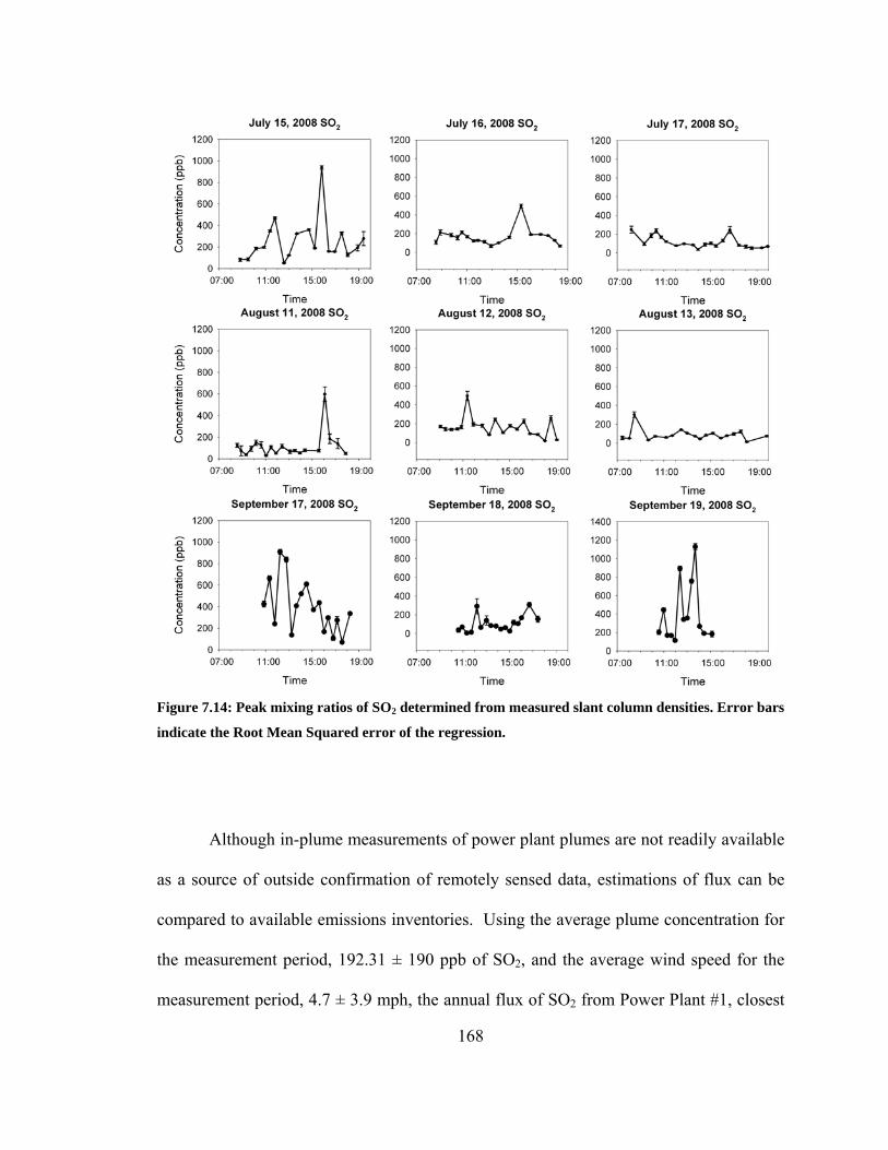
Figure 7.14: Peak mixing ratios of SO2 determined from measured slant column densities. Error bars

indicate the Root Mean Squared error of the regression.

Although in-plume measurements of power plant plumes are not readily available

as a source of outside confirmation of remotely sensed data, estimations of flux can be

compared to available emissions inventories. Using the average plume concentration for

the measurement period, 192.31 ± 190 ppb of SO2, and the average wind speed for the

measurement period, 4.7 ± 3.9 mph, the annual flux of SO2 from Power Plant #1, closest

168

169

to the sampling locations, was calculated. The size of the plume was estimated based on

the plume width, 235 m, and the approximate sampling distance downwind of the source,

900 m. Using a sampling time of 25 minutes, the annual flux of SO2 was estimated to be

1551 tons year-1. This is significantly different from the stated annual emissions of

Power Plant #1, approximate 14,000 tons year-1, from the 2008 Ohio EPA Emissions

Inventory. However, extrapolation of a full year of emissions from nine days of data

unquestionably introduces error, and, given the highly variable nature of both the wind

speed and concentrations within the plume, the estimate seems less poor. Only for an

extended period of monitoring could the variations in the type of coal being burnt and

proprietary information on the combustion rates from a particular source, as well as

variations in wind speed, be accounted for in a flux estimation. Application of the same

assumptions for NO2 yielded a flux of 71.2 tons year-1, although this measurement cannot

be compared directly to emissions data, which report only NOx. Despite the significant

discrepancies in the estimate of annual flux from the nine-day measurement period shown

here, the average concentration of SO2 for the collection period, 192.31 ± 190 ppb, is

very similar to the highest average value of SO2 for the entire measurement period, 208

ppb, obtained from AERMOD simulations. Although not as reliable as secondary

measurements within the plume itself, the agreement between these values is exceptional

given the only hourly time resolution of the AERMOD model and the limited angular

resolution of the MAX-DOAS instrument itself, and provides a measure of validation for

the methodology developed in this work.

Application of MAX-DOAS techniques to the monitoring of anthropogenic

emissions plumes is under-represented in the scientific literature. At the time of writing

170

this document, a single example was available. In that research, scans were made

perpendicular to a plume to monitor the concentration of ClO, SO2, and NO26. Based on

geometric analysis, the size of the plume was estimated, and the concentration calculated

by dividing the measured slant column densities by this plume size. Realistic values of

all three species were obtained. However, that study, published prior to the introduction

of the plume air mass factor, as proposed by Kern11 and applied in this research, neglects

the effects of radiative transfer in the horizontally in-homogeneous plume. It was found

in this work that failure to the consider the effects of radiative transfer in estimating the

concentration of SO2 and NO2 can result in concentration values, on average, 85% higher

than those methods accounting for radiative transfer, and under-estimations of NO2

concentration by an average of 5.9%. These results are not surprising, based on the

approximate order of magnitude difference in scattering efficiencies for wavelengths 413

and 305 nm, using the relationship 1/λ4. It is therefore crucial in the monitoring of SO2

plumes to account for the effects of radiative transfer.

7.10 Formaldehyde

Spectral data collected during the measurement period demonstrated strong, clear

absorptions attributed to the atmospheric species formaldehyde, HCHO. However, only

slant columns from the July 15, 2008 data set had acceptable levels of error in the

regression results. HCHO itself is not considered to be a product of coal combustion, and

is typically associated with the combustion of petroleum109. The slant column densities

of HCHO also did not show the clear plume structure (enhancement at lines of sight

pointing within the plume) demonstrated by both SO2 and NO2. Therefore, it was

assumed that the observed HCHO was not present in the plume, but rather distributed

171

throughout the atmosphere, as was the case for aerosols in this research. As such, the

radiative transfer model SCIATRAN was used to simulate the air mass factors of HCHO

for the July 15, 2008 collection period, using vertical profiles from the MPI Mainz

climatology database92. These air mass factors (differential) were subsequently used to

calculate the vertical column densities of HCHO.

From this analysis, vertical column densities of HCHO were determined from the

2.5, 5, and 7 lines of sight. Although little information can be garnered from a single day

of measurement, indeed, there is a considerable deficit in the literature on the global

distribution of HCHO in general, the average vertical column of HCHO measured from

the July 15th, 2008 was 2.3x1016 molecules cm-2. Within the available literature, only a

single point of comparison, based on the simulation of HCHO columns in North America

using the three-dimensional model GEOS-Chem. The results of this simulation predict a

vertical HCHO column of approximately 1.5x1016 molecules cm-2110:

The modeled column of HCHO over the Upper Ohio River Valley, approximately

1.5x1016 molecules cm-2, is comparable to the average measured value from July 15,

2008 over the same region. Given the deficit in available data, this comparison serves

only to confirm that the chosen analysis method, that is, simulating the air mass factors of

HCHO treating the species as horizontally homogeneous and the wavelength region

chosen for the analysis of HCHO are adequate. Further investigation and measurement

would be required to draw any further conclusions on the distribution of HCHO over this

region. However, the assumed horizontally homogeneous nature of HCHO in this region

would lend itself to the Bayesian inversion techniques presented previously for the

extinction coefficient of aerosols, should a suitable a-priori profile and spread statistics

172

become available in the future. Application of a photochemical model could produce

similar data in the absence of vertical soundings of HCHO.

173

CHAPTER 8: SUMMARY AND CONCLUSIONS

8.1 Summary

In this research, it was hypothesized that the MAX-DOAS method could be

applied to the monitoring of anthropogenic plumes, accounting fully for radiative transfer

within the isolated plume, a methodology applied previously only in theory11.

Additionally, it was hypothesized that sophisticated Gaussian plume models could be

used in both the interpretation of MAX-DOAS data collected by scanning vertically

across the height of a plume and in the evaluation of that data for accuracy. To this end,

a nine-day field study in the Upper Ohio River Valley near Wheeling, West Virginia was

conducted, during which spectra of scattered solar radiation were collected at multiple

elevation angles perpendicular to the plume of a coal-fired power plant. This data was

subsequently analyzed to determine the absorption contributions of SO2, NO2, and O4.

To ensure accurate radiative transfer simulations for the interpretation of MAX-

DOAS data, the O4 absorption signal was used in a maximum a-posteriori inversion

methodology to retrieve the vertical distribution of aerosols over the region. Based on

this inversion, an average profile of aerosol extinction coefficient at 350 nm was

obtained. This profile had a peak extinction coefficient of 0.549 km-1 at approximately

500 m above the ground. Additionally, the retrieved aerosol profiles demonstrated a

degree of correlation to changing atmospheric conditions over the course of each day, in

particular to relative humidity, a well-known controlling factor in the growth, and

174

therefore change, in aerosol extinction coefficients and optical properties15. To generate

the a-priori aerosol profile used in the inversion, the EPA regulatory model AERMOD

was used in conjunction with previous measurements of aerosol composition in the Ohio

River Valley98,102 and a model of aerosol optical properties101. The averaged extinction

coefficient profile obtained from the inversion was used in all subsequent radiative

transfer modeling applications in this research.

The spectral data collected during the nine-day field study was also analyzed to

determine the absorption contribution of NO2 and SO2, important atmospheric species

released in large amounts by coal-fired power plants. Proper interpretation of plume

data, previously based on the assumption that the light path through a plume was defined

as a straight line, required the use of a model of radiative capable of simulating the

effects of an isolated plume within an otherwise horizontally homogeneous atmosphere.

Accounting for radiative transfer within the plume itself was previously demonstrated

only in theoretical calculations, in which the concept of the Plume Air Mass Factor,

PAMF, was introduced11. In this research, PAMFs were simulated using the radiative

transfer model MCARaTS, a Monte Carlo radiative transfer program which defines the

modeling domain as a three-dimensional grid of cells, within which the concentration of a

species can be defined in each individual cell. To determine the size, shape, and altitude

of the SO2 and NO2 emissions plumes, the EPA regulatory model AERMOD was again

used to simulate the distribution of these two gases within a similar three-dimensional

grid. The plumes generated by AERMOD were based on the emissions inventory of the

facilities emitting pollutants in this region, provided by the Ohio Environmental

Protection Agency and the West Virginia Department of Environmental Protection.

175

Additional meteorological data, also used as input to the model AERMOD, were gathered

from the National Weather Service. The Plume Air Mass Factors simulated within

MCARaTS were used to convert measured slant column densities of SO2 and NO2 to

plume column densities. Based on geometric and AERMOD simulations, the size of the

plume, 235 m, was used to convert the plume column densities to mixing ratios within

the plume itself. Although a direct comparison of NO2 would only be possible using a

sophisticated chemical/physical dispersion model, the SO2 mixing ratios within the plume

can be readily compared to values obtained with the AERMOD simulation. In this case,

the measured, average concentration over the nine day sampling period was determined

to be 192.31 ± 190 ppb, and the highest average value of SO2 was determined to be 208

ppb. As stated previously, while not a direct, secondary measurement of the plume

concentration, the modeled results provide a measure of validation to the MAX-DOAS

results. Accounting for the radiative transfer within the horizontally inhomogeneous

atmosphere, in addition to giving results comparable to modeled data, can be compared to

more traditional methods of concentration estimation within a plume; that is, ignoring the

effects of radiative transfer. For the data set used in this research, failure to account for

the effects of radiative transfer yielded SO2 mixing ratios 85% higher than this method,

accounting for radiative transfer, and under-estimations of NO2 concentration by an

average of 5.9%. This is not surprising, based on the increased scattering of photons at

lower wavelengths.

In addition to SO2 and NO2, the absorption signal of HCHO, a product of

atmospheric oxidation of gaseous hydrocarbons, was analyzed. The quality of the

regression analysis for this species was quite poor and only limited information on the

176

species could be derived. In this case, the vertical column density of HCHO was

determined to be 2.3x1016 molecules cm-2, comparable to modeled results over the Ohio

River Valley110. Despite the deficit of usable data on HCHO gathered from this field

study, these preliminary results suggest firstly that the vertical profile of HCHO can be

treated as being distributed homogeneously over the region, thus lending itself to

inversion using traditional radiative transfer models and the maximum a-posteriori

inversion methodology. Secondly, the deficit of HCHO data within the literature, both

for the Ohio River Valley itself but also globally, provides ample opportunity for future

work in this field. As few profiles of HCHO have been measured vertically,

determination of the vertical distribution of this species is an ideally application of more

sophisticated physical/photochemical models.

8.2 Recommendations for Future Work

During the course of this research, shortcomings to the methodology were

recognized. Several recommendations, including modifications to the instrument,

application of emerging inversion methodologies, are given here. Firstly, the instrument

itself, initially designed as a sequential, manually operated MAX-DOAS, would benefit

greatly from the addition of automated spectral collection. For this automation to be

implemented properly, any control software must assure that the correct saturation levels

of the detector are achieved prior to collection. Secondly, rather than collecting singular

spectra at each elevation angle sequentially, a CCD array should be implemented in place

of the single row detector used in this research. In this manner, multiple telescopes, each

set to a pre-defined elevation angle, could be used, and the light collected by each

telescope directed to different regions of the CCD array by split fiber optic cables.

177

Addition of single, wide field-of-view telescope, coupled to a secondary CCD array,

would serve as a UV-visible camera, capable of imaging the plume in question.

Temporally resolved images of the plume could provide real time information on the

shape and size of the plume being proved, and would be beneficial in flux estimates

requiring plume volume estimates. Such an instrument would have a temporal resolution

limited only by the strictures of properly collecting scattered solar radiation and not the

adjustment of the elevation angle during sequential scans. Additional telescopes could

also be positioned at different azimuth angles, an emerging technique in the retrieval of

aerosol micro-physical properties using inversion methodologies7. An instrument of this

type would be capable of collecting angularly resolved spectral data with excellent

temporal resolution. The great deal of data which could theoretically be collected with

such an instrument would lend itself to emerging retrieval methodologies which do not

require the calculation of the large weighting function matrices which typify traditional

inversion methods, including the maximum a-posteriori method used in this research.

It is suggested here that Markov Chain Monte Carlo methods, implemented

previously for the inversion of oceanic circulation profiles111 and satellite data112, would

be ideal for interpreting data collected by next-generation DOAS instruments. This

method does not require the computationally intensive calculation of weighting function

matrices, nor is the method prone to converging at a local minimum on the Chi-squared

surface of the cost function, a common problem with traditional non-linear search

algorithms113. Application of the Markov Chain Monte Carlo method, coupled to a three-

dimensional radiative transfer model, could also be extended to the inversion of

horizontally in-homogeneous species, in which case the calculation of a weighting

178

function matrix would be cumbersome. Future applications of the MAX-DOAS method

to the monitoring of anthropogenic plumes should seek to improve the angular and

temporal resolution of the instrument and take advantage of emerging inversion

techniques, which can be quickly adapted to the inversion of profiles, plumes, and

microphysical properties.

179

REFERENCES

1. G. Hönninger, C. V. Friedeburg, and U. Platt, Atmospheric Chemistry and

Physics, 4, 231–254 (2004).

2. R. W. Sanders, S. Solomon, J. P. Smith, et al., Journal of Geophysical

Research, 98, 7219-7228 (1993).

3. C. D. Rodgers, Reviews of Geophysics and Space Physics, 13, 609-624 (1976).

4. C. D. Rodgers, Inverse Methods for Atmospheric Sounding: Theory and

Practice, World Scientific, Singapore, 2000.

5. B. Galle, C. Oppenheimer, A. Geyer, et al., Journal of Volcanology and

Geothermal Research, 119, 241-254 (2002).

6. C. Lee, Y. J. Kim, H. Lee, et al. in Advanced Environmental Monitoring; Y. J.

Kim, and U. Platt, Eds.; Springer, 2008.

7. T. Wagner, B. Dix, C. v. Friedeburg, et al., Journal of Geophysical Research,

109(2004).

8. S. E. Schwartz, Science, 243, 753-763 (1989).

9. B. F. Taubman, J. C. Hains, A. M. Thompson, et al., Journal of Geophysical

Research, 111(2006).

10. S. E. Schwartz, and M. O. Andreae, Science, 272, 1121-1122 (1996).

180

11. C. Kern, T. Deutschmann, L. Vogel, et al., Bulletin of Volcanology, 71(2009).

12. D. J. Jacob, Introduction to Atmospheric Chemistry, Princeton University

Press, Princeton, New Jersey, 1999.

13. M. Hausmann, U. Brandenburger, T. Brauers, et al., Journal of Geophysical

Research, 102, 16011-16022 (1997).

14. B. J. Finlayson-Pitts, and J. N. Pitts Jr., Chemistry of the Upper and Lower

Troposphere, Academic Press, SanDiego, California, 2000.

15. J. H. Seinfeld, and S. N. Pandis, Atmospheric Chemistry and Physics: From

Air Pollution to Climate Change, John Wiley and Sons, Inc., New York, 1998.

16. C. Hak, I. Pundt, S. Trick, et al., Atmospheric Chemistry and Physics, 5, 2881-

2900 (2005).

17. COESA. NOAA, 1976, p 227.

18. S. Chandrasekhar, Radiative Transfer, Dover, New York, 1960.

19. L. C. Henyey, and J. L. Greenstein, Astrophysics Journal, 93, 70-83 (1941).

20. H. Iwabuchi, Journal of the Atmospheric Sciences, 63, 2324-2339 (2006).

21. A. Rozanov, V. Rozanov, M. Buchwitz, et al., Advances in Space Research, 36,

1015-1019 (2005).

22. A. Rozanov, V. Rozanov, and J. P. Burrows, Journal of Quantitative

Spectroscopy and Radiative Transfer, 69, 491-512 (2001).

23. V. V. Rozanov, K.-U. Eichmann, R. de Beek, et al., Advances in Space

Research, 29, 1831-1835 (2002).

24. A. Rozanov, V. Rozanov, and J. P. Burrows, Jounal of Geophysical Research,

105, 22937-22943 (2000).

181

25. D. A. Skoog, F. J. Holler, and T. A. Nieman, Principles of Instrumental

Analysis, Saunders College Publishing, 1971.

26. J. M. C. Plane, and N. Smith. in Spectroscopy in Environmental Science; R. J.

H. Clark, and R. E. Hester, Eds.; John Wiley and Sons, Inc., 1995.

27. U. Platt. in Air Monitoring by Spectroscopic Techniques; M. W. Sigrist, Ed.;

John Wiley and Sons, New York, 1994, p 27-84.

28. C. Frohlich, and G. E. Shaw, Applied Optics, 19, 1773-1775 (1980).

29. D. R. Bates, Planetary and Space Science, 32, 785-790 (1984).

30. U. Platt, D. Perner, and H. W. Patz, Journal of Geophysical Research, 84,

6329-6338 (1979).

31. U. Platt, and D. Perner, Springer Ser. Opt. Sci., 39, 95-105 (1983).

32. J. M. C. Plane, and C.-F. Nien, Rev. Sci. Instrum., 63, 1867-1876 (1992).

33. D. Perner, and U. Platt, Geophysical Research Letters, 6, 917-920 (1979).

34. J. D. Ingle, and S. R. Crouch, Spectrochemical Analysis, Prentice Hall, Upper

Sadle River, New Jersey, 1988.

35. H. Okabe, Photochemistry of Small Molecules, Wiley-Interscience, New York,

1978.

36. H. Keller-Rudek, and G. K. Moortgat. Max-Planck-Institut für Chemie,

Atmospheric Chemistry Division, Mainz, Germany.

37. B. A. Thompson, P. Harteck, and R. R. R. Jr., Jounal of Geophysical

Research, 68, 6431-6436 (1963).

38. S. Voigt, J. Orphal, and J. P. Burrows, Journal of Photochemistry and

Photobiology A: Chemistry, 149, 1-7 (2002).

182

39. J. Stutz, E. S. Kim, U. Platt, et al., Jounal of Geophysical Research, 105,

14585-14592 (2000).

40. K. Bogumil, J. Orphal, T. Homann, et al., Journal of Photochemistry and


41. C. A. Cantrell, J. A. Davidson, A. H. McDaniel, et al., Journal of Physical

Chemistry, 94, 3902-3908 (1990).

42. T. Etzkorn, B. Klotz, S. Sørensen, et al., Atmospheric Environment, 33, 525-

540 (1999).

43. F. G. Simon, W. Schnieder, G. K. Moortgat, et al., Journal of Photochemistry

and Photobiology A: Chemistry, 55, 1-23 (1990).

44. D. M. Wilmouth, T. F. Hanisco, N. M. Donahue, et al., Journal of Physical

Chemistry, 103, 8935-8945 (1999).

45. S. Voigt, J. Orphal, K. Bogumil, et al., Journal of Photochemistry and

Photobiology A: Chemistry, 143(2001).

46. G. D. Greenblatt, J. J. Orlando, J. B. Burkholder, et al., Journal of

Geophysical Research, 95, 18577-18582 (1990).

47. G. W. Kattawar, A. T. Young, and T. J. Humphreys, The Astrophysical

Journal, 243, 1049-1057 (1981).

48. D. J. Fish, and R. L. Jones, Geophysical Research Letters, 22, 811-814 (1995).

49. G. Barrefors, The Science of the Total Environment, 189/190, 287-292 (1996).

50. S. R. Aliwell, M. V. Roozendael, P. V. Johnston, et al., Journal of Geophysical

Research, 107, 10-11-10-20 (2002).

183

51. J. Stutz, R. Ackermann, J. D. Fast, et al., Geophysical Research Letters,

29(2002).

52. P. K. Dasgupta, J. Li, G. Zhang, et al., Environmental Science and

Technology, 39, 4767-4783 (2004).

53. A. Heckel, A. Richter, T. Tarsu, et al., Atmospheric Chemistry and Physics, 5,

909-918 (2005).

54. Y. Yoshii, H. Kuze, and N. Takeuchi, Applied Optics, 42, 4362-4368 (2003).

55. Y. Xue, J. Niu, W. Liu, et al., Japanese Journal of Applied Physics, 39, 622-

627 (2000).

56. C. v. Friedeburg, I. Pundt, K.-U. Mettendorf, et al., Atmospheric

Environment, 39, 977-985 (2005).

57. B. J. Allan, J. M. C. Plane, H. Coe, et al., Journal of Geophysical Research,

107(2002).

58. J. F. Noxon, R. B. Norton, and W. R. Henderson, Geophysical Research

Letters, 5, 675-678 (1978).

59. T. Wagner, C. Otten, K. Pfeilsticker, et al., Geophysical Research Letters, 27,

3441-3444 (2000).

60. U. Platt, L. Marquard, T. Wagner, et al., Geophysical Research Letters, 24,

1759-1762 (1997).

61. S. Solomon, A. L. Schmeltekopf, and R. W. Sanders, Geophysical Research

Letters, 92, 8311-8319 (1987).

62. A. Petritoli, F. Ravegnani, G. Giovanelli, et al., Applied Optics, 41, 5593-5599

(2002).

184

63. T. Wagner, C. v. Friedeburg, M. Wenig, et al., Journal of Geophysical

Research, 107(2002).

64. R. Sinreich, U. Frieß, T. Wagner, et al., Faraday Discussions, 130, 153-164

(2005).

65. P. Wang, A. Richter, M. Bruns, et al., Atmospheric Chemistry and Physics, 6,

329-338 (2006).

66. N. Bobrowski, G. Honninger, B. Galle, et al., Nature, 423, 273-276 (2003).

67. J. Stutz, and U. Platt, Applied Optics, 35, 6041-6053 (1996).

68. D. Goorvitch, Journal of Quantitative Spectroscopy and Radiative Transfer, 67,

253-257 (2000).

69. E. Hecth, Optics, Addison Wesley, San Francisco, California, 2002.

70. S. W. Smith, The Scientist and Engineer's Guide to Digital Signal Processing,

California Technical Publishing, San Diego, California, 1997.

71. W. H. Press, S. A. Teukolsky, W. T. Vetterling, et al., Numerical Recipes in C:

The Art of Scientific Computing, Cambridge University Press, Cambridge, 1988.

72. SCIATRAN. Institute of Remote Sensing, University of Bremen, Germany,

Bremen, Germany, 2007.

73. M. van Roozendael, and C. Fayt, (2001).

74. H. K. Roscoe, D. J. Fish, and R. L. Jones, Applied Optics, 35, 427-432 (1996).

75. C. Caspar, and K. Chance. Third European Remote-Sensing Satellite

Scientific Symposium: Space at the Service of Our Environment, The Netherlands,

1997, pp 609-614.

76. J. H. G. M. van Geffen, and R. F. v. Oss, Applied Optics, 42, 2739-2753 (2003).

185

77. J. F. Noxon, Science, 189, 547-549 (1975).

78. D. L. Albritton, A. L. Schmeltekoph, and R. N. Zare. in Molecular

Spectroscopy: Modern Research; K. N. Rao, Ed.; Academic Press, New York, 1976, p

1-67.

79. OceanOptics. Ocean Optics, Incorporated, Dunedin, FL, 2007.

80. P. Pelikan, M. Ceppan, and M. Liska, Applications of Numerical Methods in

Molecular Spectroscopy, CRC Press, Boca Raton, 1994.

81. M. Vountas, V. V. Rozanov, and J. P. Burrows, Jounal of Quantitative


82. K. V. Chance, and R. J. D. Spurr, Applied Optics, 36, 5224-5230 (1997).

83. M. Wenig, B. Jahne, and U. Platt, Applied Optics, 44, 3246-3252 (2005).

84. M. Hausmann, U. Brandenburger, T. Brauers, et al., Applied Optics, 36, 462-

475 (1999).

85. J. Stutz, and U. Platt, Applied Optics, 36, 1105-1115 (1997).

86. N. Smith, J. M. C. Plane, C.-F. Nien, et al., Atmospheric Environment, 29,

2887-2897 (1995).

87. J. Harder, and G. H. Mount. in Remote Sensing of Atmospheric Chemistry; J.

L. McElroy, and R. J. McNeal, Eds.; SPIE, 1991.

88. L. C. Marquard, T. Wagner, and U. Platt, Journal of Geophysical Research,

105, 1315-1327 (2000).

89. C. v. Friedeburg. in Natural Sciences and Mathematics; Ruperto-Carola

University of Heidelberg, Heidelberg, Germany, 2003, p 244.

186

90. T. Wagner, J. P. Burrows, T. Deutschmann, et al., Atmospheric Chemistry

and Physics, 7, 1809-1833 (2007).

91. R. Schofield, B. J. Connor, K. Kreher, et al., Journal of Quantitative


92. C. Bruhl, and P. J. Crutzen. in The Atmospheric Effects of Stratospheric

Aircraft, Nasa Reference Publication 1993, 1993, p 103-104.

93. M. J. Reider, and G. Kirchengast, Radio Science, 35, 45-56 (2000).

94. A. N. Tikhonov, Dokl. Acad. N., 151, 501-504 (1963).

95. S. Twomey, Journal of the Association for Computing Machinery, 10, 97-101

(1963).

96. M. Edmonds, R. A. Herd, B. Galle, et al., Bulletin of Volcanology, 65, 578-586

(2003).

97. G. G. Salerno, M. R. Burton, C. Oppenheimer, et al., Journal of Volcanology

and Geothermal Research, 181, 141-153 (2009).

98. R. L. N. Yatavelli, J. K. Fahrni, M. Kim, et al., Atmospheric Environment, 40,

6650-6665 (2006).

99. D. Perner, and U. Platt, Geophysical Research Letters, 7, 1053-1056 (1980).

100. USEPA. U. S. Environmental Protection Agency Office of Air Quality

Planning and Standards, Emissions Monitoring and Analysis Division, Research

Triangle Park, North Carolina, 2004.

101. M. Hess, P. Koepke, and I. Schult, Bulletin of the American Meteorological

Society, 79, 831-844 (1998).

187

102. M. Kim, S. R. Deshpande, and K. C. Crist, Atmospheric Environment, 41,

9231-9243 (2007).

103. B. A. Schichtel, R. B. Husar, S. R. Falke, et al., Atmospheric Environment, 35,

5205-5210 (2001).

104. A. Horowitz, R. Meller, and G. K. Moortgat, Journal of Photochemistry and


105. O. C. Fleischmann, M. Hartmann, J. P. Burrows, et al., Journal of

Photochemistry and Photobiology A: Chemistry, 168, 117-132 (2004).

106. S.-C. Yoon, and J. Kim, Atmospheric Environment, 40, 4328-4338 (2006).

107. N. V. Gillani, and W. E. Wilson, Annals of the New York Academy of Sciences,

38, 276-296 (1980).

108. A. C. Vandaelea, A. Tsoulib, M. Carleerb, et al., Environmental Pollution,

116, 193–201 (2002).

109. B. P. Wert, M. Trainer, A. Fried, et al., Jounal of Geophysical Research, 108,

8.1-8.14 (2003).

110. D. B. Millet, D. J. Jacob, S. Turquety, et al., Journal of Geophysical Research,

111(2006).

111. I. W. McKeague, G. Nicholls, K. Speer, et al., Journal of Marine Research, 63,

683-704 (2005).

112. H. Haario, M. Laine, M. Lehtinen, et al., Journal of the Royal Statistical

Society, 66, 591-607 (2004).

113. L. Tierney, The Annals of Statistics, 22, 1701-1728 (1994).

Differential Optical Absorption Spectroscopy of … Optical Absorption Spectroscopy of Trace Gas...

Documents

Transcript of Differential Optical Absorption Spectroscopy of … Optical Absorption Spectroscopy of Trace Gas...