Differential Expression Analysis: RNA-Seq

2011 Winter School in Mathematical and Computational Biology!Tuesday, 5 July 2011!

Davis McCarthy!Bioinformatics Division!

Walter + Eliza Hall Institute of Medical Research!

Study development: same DNA, different form/function

Source: Wikipedia 2

Find genes driving disease

DNA Sequence Ain’t Everything

RNA-Seq

•  Use of ultra high-throughput sequencing (‘next-’ or ‘second’-generation) technologies for the study of gene expression

•  Discover gene activity and function by finding differentially expressed genes

•  My focus: statistical methods for differential expression analysis

3

DE Analysis is Crazy (Statistically Speaking)

•  Make inference on DE for ~20,000 genes…simultaneously…from 6 samples

•  Ultra high-dimensional data •  Degrees of freedom? •  Analytical methods still open research

4

The Point!•  Good DE analysis of RNA-Seq data requires:!

1.  Good statistical models for DE!2.  Understanding and proper modeling of the

variability in RNA-seq data!3.  Efficient, useable statistical software !

•  Negative Binomial GLM methods can be used to analyze complex experimental designs while accounting for biological variation!

•  edgeR software implements these methods !

5

DE Analysis Happens in R •  R: free, open-source statistical software •  Bioconductor: repository for free, open-source, R

packages for bioinformatics •  Several packages currently available for DE analysis

of RNA-seq data in R: –  baySeq [Hardcastle & Kelly, 2010] –  DEGSeq [Wang et al, 2010] –  DESeq [Anders & Huber, 2010] –  edgeR [Robinson, McCarthy & Smyth, 2010] –  NBPSeq [Di et al, 2011] (+ more methods with less refined code, e.g. TSPM [Auer

& Doerge, 2011]) •  I work on edgeR, so this is my favourite •  edgeR is only package so far with full GLM capabilities

6

Outline

1.  RNA-Seq and Models for Differential Expression

2.  Accounting for Biological Variation 3.  NB GLMs in edgeR Handle Complex

Designs 4.  Case Study: Paired Design Tumour vs

Normal

7

RNA-SEQ AND DE MODELS

High-throughput sequencing, RNA-Seq, Count Data, Statistical Models, Current State of Play

8

Differential expression (DE) testing

Fig: Oshlack, Robinson & Young, Genome Biology, 2010

9

Long pipeline to go from reads to results in an RNA-Seq study

RNA-Seq Data for DE Analysis is a Table of Counts

Tag ID! A1! A2! B1! B2!ENSG00000124208! 478! 619! 4830! 7165!ENSG00000182463! 27! 20! 48! 55!ENSG00000125835! 132! 200! 560! 408!ENSG00000125834! 42! 60! 131! 99!ENSG00000197818! 21! 29! 52! 44!ENSG00000125831! 0! 0! 0! 0!ENSG00000215443! 4! 4! 9! 7!ENSG00000222008! 30! 23! 0! 0!ENSG00000101444! 46! 63! 54! 53!ENSG00000101333! 2256! 2793! 2702! 2976!

…! … tens of thousands more tags …!

** very high dimensional data ** 10

We Assess DE for Each Gene

•  For EACH GENE, is the mean expression level for the gene under one condition significantly different from the mean expression level under a different condition?

Tag ID! A1! A2! B1! B2!ENSG00000124208! 478! 619! 4830! 7165!ENSG00000182463! 27! 20! 48! 55!ENSG00000125835! 132! 200! 560! 408!ENSG00000125834! 42! 60! 131! 99!

…! … tens of thousands more tags …!

11

Model Variability to Assess DE

•  Want to assess DE for ~20 000 genes simultaneously

•  Which differences are real, which likely to have appeared by chance?

•  Answer this question with a statistical model for DE

•  Need to understand variability and model it appropriately

12

Significance of Differences Depends on Variability of Samples

13

!!

!

!!!!!

!!

!

!

!!

!

!

020

4060

8010

0

Low variance samplesR

ead

coun

t

x

x

mean=49 sd=6

mean=73 sd=5

Difference in means unlikely due to chance

!

!

!

!!

!!

! !

!

!

!

!

!

!

!

050

100

200

300

High variance samplesR

ead

coun

t

xx

Significance of Differences Depends on Variability of Samples

14

mean=61 sd=62

mean=114 sd=119

Difference in means

more likely due to chance

There are Several Options for Creating a Model for DE for Count Data

Transform count data and apply standard methodology: •  Gaussian (normal) model using transformed counts (e.g. log transform)

Analyze using models for count data: •  Poisson •  Negative binomial (NB) + other possibilities

Whatever approach we take, we must account for biological variation

15

Test DE by Fitting a Model for Each Gene

•  Fit a statistical model for DE to each gene, accounting for biological variability

•  Test null hypothesis of zero DE against alternative of some DE

•  Tens of thousands of hypothesis tests •  Multiple testing (usu. control FDR)

16

ACCOUNTING FOR BIOLOGICAL VARIATION

Importance of variance model, Technological & Biological Variation, Coefficient of Variation, Negative Binomial Model

17

RNA-Seq Data Exhibits Technical and Biological Variation

•  Two levels of variation in any RNA-Seq experiment

1.  Relative abundance (expression level) of each gene will vary between RNA samples, due mainly to biological causes.

2.  There is measurement error – uncertainty with which the abundance of each

gene in each sample is estimated by the sequencing technology.

18

19

Counts from a Single RNA Sample Can be Modeled with Poisson Distribution

RNA sample

M = total number of reads ≈ 20 million λg = true proportion of gene g yg = number of reads for gene g

Read 1 Read 2 Read 3 Read 4 Read 5 Read 6 …

Short reads

Map reads to genome

What we’re interested in

What we observe

Large M, small λi yg approximately Poisson, µg = Mλg

20

A Small RNA-Seq Experiment (Tech Reps)

RNA from stem cells RNA from luminal cells

λg1 λg2

λg3 λg4

yg1 yg2 yg3 yg4

Genes g = 1, …, 30k

M1 M2

M3 M4

E(ygi) = Mi λgi Reads Mi ≈ 20 million

True Technical Reps Show Poisson Variation for Each Gene

Data: Marioni et al., Genome Res, 2008

21 binned variance, sample variance

Liver tissue vs kidney tissue

22

A Small RNA-Seq Experiment (Biological Reps)

RNA from stem cells RNA from luminal cells

λg1 λg2

λg3 λg4

yg1 yg2 yg3 yg4

Genes g = 1, …, 30k

M1 M2

M3 M4

E(ygi) = Mi λgi Reads Mi ≈ 20 million

Poisson Sequencing Variation Leads to Coefficient of Variation

•  Technical replicate counts for a gene vary according to a Poisson law, i.e. sequencing variation is Poisson

•  Biological CV (BCV) is the coefficient of variation with which the (unknown) true abundance of the gene varies between RNA samples.

•  Let BCV2 = φ •  If you can determine BCV then you have a quadratic

mean-variance relationship var(ygi)= µgi + φgµgi

2 with φg=Biological CV2

23

Biological Coefficient of Variation Dominates Technical

•  Separate biological and technical variation •  Technical CV decreases as size of counts increases.

BCV does not. •  BCV likely to be the dominant source of uncertainty for

high-count genes •  Reliable estimation of BCV is crucial for realistic

assessment of DE in RNA-Seq experiments.

CV2(ygi) = var( ygi ) / µgi2 = 1/µgi + φg

24

Total CV2 = Technical CV2 + Biological CV2

Biological Replicate Data shows Quadratic Mean-Variance Relationship

(development cycle of slime mould, 2 samples at hr00, & 2 at hr04)

binned variance, sample variance

Data: Parikh et al, Genome Biology, 2010

BCV = 0.38

25

Quadratic Mean-Variance Relationship Leads to Negative Binomial Model

•  (With a couple of assumptions) counts follow a negative binomial distribution

E(ygi) = Mi λgi, ygi ~ NegBin( µgi, φg)

•  Reasonable model for DE in RNA-seq data that accounts for biological variation

26

NB GLMS IN EDGER HANDLE COMPLEX DESIGNS

Generalized Linear Models, NB Model, Estimating BCV, Flexibility

27

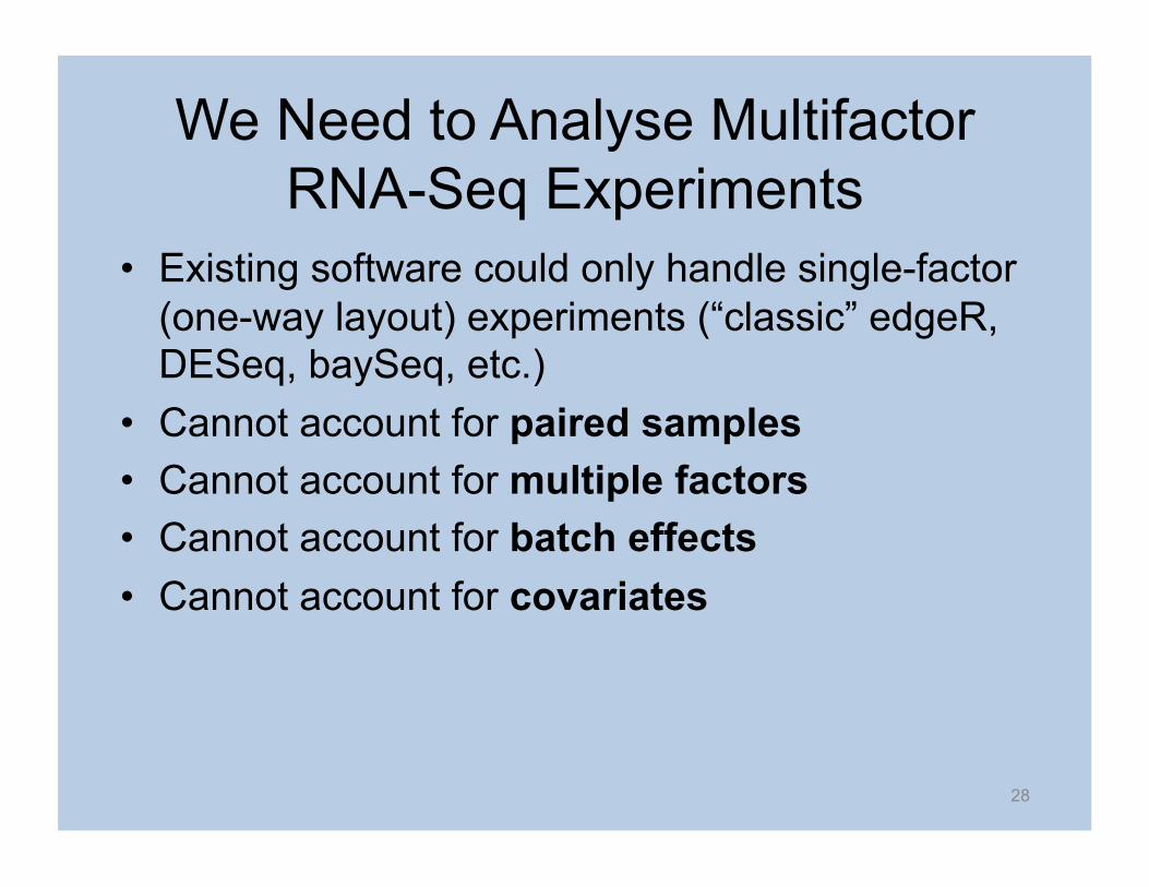
We Need to Analyse Multifactor RNA-Seq Experiments

•  Existing software could only handle single-factor (one-way layout) experiments (“classic” edgeR, DESeq, baySeq, etc.)

•  Cannot account for paired samples •  Cannot account for multiple factors •  Cannot account for batch effects •  Cannot account for covariates

28

Inference on Differentially Expressed Genes May Be Wrong If Information Ignored

29

!

!

!

!

!

!

1 2 3 4 5 6

020

4060

8010

0

Sample

Rea

d co

unt Normal

Cancer

Difference between cancer and normal samples looks not significant

!

!

!

!

!

!

1 2 3 4 5 6

020

4060

8010

0

Sample

Rea

d co

unt

Differentially Expression Found When Accounting for Patient Effect

30

Patient 1 Patient 2 Patient 3

Cancer Normal

2-fold difference between cancer and normal within each patient

GLM Methods Are Flexible

•  GLM (generalized linear model) approach handles complicated designs – any design that can be expressed as a linear model

•  Fit full model and a null (smaller) model to the data to each gene (i.e. fit 20,000 models)

•  Use a likelihood-ratio test to determine DE •  GLM methods apply to NB distribution

31

Sharing Information Across Genes Improves BCV Estimation

•  Variance structure (BCV) estimated from dataset as a whole

•  Stabilize estimates & inference – important for small sample sizes

•  Common BCV for all genes – estimated from all of the data

•  Common conditional likelihood •  Acts like a Bayesian prior distribution

32

edgeR Overcomes Issues with Estimating BCV

•  In edgeR we allow BCV that: –  varies between genes (“tagwise”), and –  shows a systematic trend with respect to gene

expression •  Weighted likelihood (cf empirical Bayes) to

obtain genewise BCVs squeezed towards common BCV

•  Cox-Reid APL (approx. conditional inference) used to estimate common/trended/genewise BCV for GLMs

33

NB GLM methods can be used to analyse multifactor experiments while accounting for

biological variation

34

CASE STUDY: PAIRED DESIGN TUMOUR VS NORMAL

NB GLMs improve the analysis of an RNA-Seq experiment studying differential expression from paired oral squamous cell carcinoma and normal oral tissue samples from 3 patients

35

We Aim to Find Genes DE between Normal and Tumour, Accounting for Patient Effects

•  RNA-seq data from Tuch et al (2010) – SOLiD v3.0 •  Comparing oral squamous cell carcinoma tissue to

matched healthy oral tissue •  6 samples, paired design

Normal Tumour Patient 8 N8 T8 Patient 33 N33 T33 Patient 51 N51 T51

36

Include Patient and Tissue Effects in Additive GLM Approach

•  A log-linear model fitted to the counts ygi for each gene

•  Model includes a patient factor (three levels) and a tissue factor (tumour & normal)

•  We can estimate the baseline patient expression levels for each gene.

•  Likelihood ratio tests are used to test the null hypothesis that the tumour vs normal log-fold change for each gene is zero (after accounting for patient effects)

37

Including Patient Effect Reduces BCV Estimate

•  Cox-Reid takes experimental design into account when estimating BCV –  corrects for baseline differences between patients

•  Estimated (common) BCV = 40% •  True expression levels show substantial biological

variability, even accounting for patient effects •  Treating the three tumour samples as independent

replicates would yield a higher BCV of 52% •  Paired design is successful in correcting for some

patient to patient variation – increases power

38

Common BCV is Too Simple: Substantial subset of genes shows strong evidence of greater variability than implied by common BCV

Data: Tuch et al., 2008 39

Tagwise BCV Gives Best Overall Fit to These Data

Deviance goodness of fit statistics transformed to normality for QQ-plot

•  Common BCV rejected for 39 genes at a family-wise error rate of 0.05 •  Allowing an abundance trend on the BCV does not reduce the number of outlier genes for which the BCV is rejected, but tagwise BCV drastically does •  Poisson model rejected for 72% of genes (not shown)

40

GLM Approach Compares Favourably to Original Analysis

•  A more formal analysis that assesses statistical significance relative to biological variation

•  GLM approach finds more DE genes with statistical evidence

•  GLM approach yields biologically relevant DE genes

41

CONCLUSION Software Implementation, Applications, Final Points

42

NB GLMs Show Great Utility for DE Analysis of RNA-Seq Data

•  NB GLMs can be used to analyse differential expression in multifactorial RNA-Seq experiments while accounting for biological variation.

•  Case studies show these methods to be useful on small and large datasets with very different characteristics

•  Implementation in the edgeR package offers flexible, highly efficient statistical tools

43

Special Acknowledgement

•  Yunshun (Andy) Chen: PhD student, WEHI Bioinformatics – Cox-Reid APL (estimating BCV for GLMs) – making the GLM fit secure (line search etc.) + much more

44

45

Acknowledgements!WEHI Bioinformatics

Gordon Smyth Yunshun Chen Mark Robinson Terry Speed edgeR Users

Thanks!