1

Proceedings of IDETC/CIE 2007 ASME 2007 International Design Engineering Technical Conferences & Computers and Information in Engineering

Conference September 4-7, 2007, Las Vegas, Nevada, USA

DETC2007-34290

DIFFERENTIAL EVOLUTION APPLIED TO THE DESIGN OF A THREE-DIMENSIONAL VEHICULAR STRUCTURE

Felipe Antonio Chegury Viana

fchegury@mecanica.ufu.br

Fernando César Gama de Oliveira

fcoliveira@mecanica.ufu.br

Jose Antonio Ferreira Borges

zeborges@mecanica.ufu.br

Valder Steffen, Jr*

vsteffen@mecanica.ufu.br

School of Mechanical Engineering Federal University of Uberlândia

Avenida João Naves de Ávila, 2121, Uberlândia, MG, Brazil 38400-902

* Professor and author of correspondence, Phone: +55 (34) 3239-4148, Fax: +55 (34) 3239-4206

ABSTRACT

The purpose of this paper is to demonstrate the application

of Differential Evolution to a realistic design optimization test

problem. The present contribution regards the improvements

implemented to the original basic algorithm as well as the

application of a new algorithm for dealing with the unique

challenges associated with real world optimization problems.

The selected example is a three-dimensional vehicular structure

optimization problem modeled using the commercial Finite

Element software ANSYS® that has a combination of

continuous and discrete design variables. The use of traditional

gradient-based optimization algorithms is thus not practical.

The numerical results presented indicate that the Differential

Evolution algorithm is able to find the optimum design for the

proposed problem. The algorithm is robust in the sense that it is

capable of dealing with the numerical noise involved in the

modeling of the system and to manipulate discrete design

variables, accordingly.

1 INTRODUCTION According to Venter and Sobieski in [1], in the recent years

non-gradient based, probabilistic search algorithms have

attracted much attention from the scientific community. Even

though classical methods (where the search process is guided by

information about the gradient) have been widely used due to

their computational efficiency, they have difficulties when a

local minimum is found. It is quite often erroneously interpreted

as the global one. In the other hand, nature-inspired methods are

in general zero-order methods, and consequently they do not

need information about the gradient. These algorithms generally

mimic some natural phenomena, for example Ant Colony

Optimization (ACO), Genetic Algorithms (GA) and Particle

Swarm Optimization (PSO). ACO is inspired in the behavior of

real ants and their communication scheme by using pheromone

trail; GA models the evolution of a species as based on Darwin's

principle of survival of the fittest; while PSO reproduces the

search procedure used by a swarm of birds when looking for

food. They have several advantages, such as easiness to code,

robustness, efficiency in making use of parallel computing

architectures, and trend to find the global, or near global,

solution. As a consequence of the large number of function

evaluations required by the algorithm, this is seen as a

disadvantage of this type of method, due to heavy

computational effort usually observed [2].

In this paper, a recent type of heuristic, named Differential

Evolution (DE) is investigated. The DE algorithm was first

introduced by Storn and Price [3], [4] as a method of

mathematical optimization of multidimensional functions. The

present paper focuses on enhancements to the basic DE

algorithm. These include the introduction of a set of

convergence criteria, dealing with multi-objective and

constrained optimization problems, discrete problems,

additional randomness, and composed DE schemes. The

enhanced version of the algorithm is applied to the design of a

three-dimensional vehicular structure encompassing one

discrete and thirty two continuous design variables.

2

2 BASIC DIFFERENTIAL EVOLUTION OPTIMIZATION ALGORITHM

Even though the DE community has adopted biological terms to

describe arithmetic operations on real (and discrete) variables,

i.e., mutation and recombination, the operations are more akin

to dynamics/thermodynamics and physics than they are to

biology. Selection is perhaps the DE's most Darwinian aspect,

but even here, competition for survival is more limited than in

most evolutionary algorithms. The main idea behind DE is how

possible solutions taken from the population of individuals are

set, recombined and chosen to evolve the population to the next

generation. This way, the weighted-difference scheme seems to

be the most important feature of the present heuristic.

2.1 Algorithm Description

In a population of individuals (seen as potential solutions), a

fixed number of vectors are randomly initialized, and then

evolved over the optimization task to explore the design space

and hopefully to locate the optimum of the objective function.

Each iteration new vectors are generated by the combination of

vectors that are randomly chosen from the current population

(this is also referred to as “mutation” in the DE literature). The

out coming vectors are then mixed with a predetermined target

vector. This operation is called “recombination” and produces a

“trial vector”. Finally, the “trial vector” is accepted for the next

generation if and only if it yields a reduction in the value of the

objective function. This last operator is referred to as

“selection”. As can be seen, the basic algorithm preserves some

common aspects of the traditional simple GA (specially the

nomenclature of some operators, such as selection, crossover

and mutation).

In terms of representation, a population of m individuals is

expressed as a m n× matrix, [ ]1 2, , ,

T

m= …P x x x where

[ ]1 2, , ,

T

nx x x=x … is a vector of design variables that

corresponds to a single individual. The outline of a basic DE is

as shown in Figure 1.

The DE community has established the following notation to

determine how the mutation and crossover operators work

together [3], [4]: DE/x/y/z

where:

• x specifies the vector to be mutated, which currently can be

one of the following:

− “rand”: a randomly chosen population vector,

− “best”: the vector of best objective value from the

current population,

− “rand-to-best”: this scheme takes both a randomly

chosen individual and the best one.

• y is the number of difference vectors used, and

• z denotes the crossover scheme, which can be either “bin”

(independent binomial experiments) or “exp” (exponential

crossover).

Figure 1. Basic scheme for DE.

2.2 Mutation

As described before, the DE mutation is the operator that first

adds the weighted difference between two individuals to a third

individual. Table 1 gives more details about each mutation

scheme.

Table 1. Different implementations of the DE mutation.

Type Updating

Equation

Target

Vector

Population

Size

“rand/1” 1 2 3( )

trial r r rF= + −x x x x

1rx 3>

“rand/2” 1

2 3 4 5( )

trial r

r r r rF

= +

− + −

x x

x x x x 1r

x 5>

“best/1” 2 3( )

trial best r rF= + −x x x x

bestx 3>

“best/2”

1 2 3 4( )

trial best

r r r rF

= +

− + −

x x

x x x x best

x 5>

“rand-to-

best/1” 1 2( )

trial

best r rF

= +

− + −

x x

x x x x x 5>

“rand-to-

best/2” 1 2 3 4

( )

( )

trial best

r r r r

F

F

= + − +

− + −

x x x x

x x x x x 6>

where:

• trial

x is the trial vector (individual);

• { }1, 2, 3, 4, 5 1, 2, ,r r r r r m∈ … are random integer

indexes and mutually different;

• F is a real constant factor [ ] 0, 2∈ , which controls the

amplification of the differential variation;

3

• best

x is the best individual of the current population; and

• x is the current individual.

In DE, mutation is the first step of the design variable

update. The complement of this process is done by the

crossover operator. There are two types of crossovers: binary

and exponential. The superiority of each crossover scheme over

the other can not be uniquely defined, which means that this is a

problem-dependent operator. In other words, a strategy that

works out to be the best for a given problem may not work well

when applied to a different problem. Thus, the final trial vector,

trialx , is formed in such a way that the i-th coordinate is given

by:

, if crossover is applicable,

, otherwise

1, 2, , .

mutation

ì

trial

i

xx

x

i n

=

= …

(1)

In practical terms, DE has a parameter that controls the

crossover, namely the crossover probability, CR . In

exponential crossover, the crossover is performed in a loop

controlled by a uniform random number, rn and a counter that

ranges from 0 to n−1. The first time a randomly picked number

between 0 and 1 goes beyond the CR value, no crossover is

performed and the remaining of the n variables are left intact

[3], [4], [5]. Table 2 shows a C-like pseudo-code for the

exponential crossover.

Table 2. Pseudo-code for the DE exponential crossover.

counter = 0;

do{

rn = rand();

if (rn < CR) {

x(counter) = xmutation(counter);

}

counter = counter + 1;

}while( (rn < CR) and (counter < n) );

In the binomial crossover, the operation is performed on

each of the n variables whenever a randomly picked number

between 0 and 1 is lesser than the CR value [3], [4], [5]. Table

3 shows a C-like pseudo-code for the binomial crossover.

It can be noticed that for high values of CR, the exponential

and binomial crossovers yield similar results.

2.3 Selection

Selection is the simplest DE operator. It is used to decide

whether of not the new vector,new

x , should become a member

of the next generation. The approach is straightforward: the

objective function value of the new individual, ( )new

f x , is

compared with the one of the target vector, target

( )f x . If there is

an improvement, new

x is set to the next generation; otherwise,

targetx is retained.

Table 3. Pseudo-code for the DE binomial crossover.

counter = 0;

do{

rn = rand();

if (rn < CR) {

x(counter) = xmutation(counter);

}

counter = counter + 1;

}while( counter < n );

2.4 Remarks about DE

Storn in [5] gives a set of practical rules useful when it comes to

choose the DE parameters, namely:

• A population size of 10 times the number of design

variables is a good choice for many applications.

• Most often the crossover probability, CR , must be

considerably lower than one (e.g. 0.3). However, if no

convergence can be achieved, [ ] 0.8, 1CR ∈ should be

tried. This is especially true when using exponential

crossover.

• The higher the population size is chosen, the lower the

weighting factor F .

• F is usually chosen [ ] 0.5, 1∈ .

Last but not least, it is worth mentioning that combining the

six mutation schemes shown in Table 1 with the two previously

presented crossover schemes, it can be explored a total number

of twelve DE strategies. By following the DE/x/y/z notation:

DE/rand/1/bin, DE/rand/1/exp, DE/rand/2/bin, DE/rand/2/exp,

DE/best/1/bin, DE/best/1/exp, DE/best/2/bin, DE/best/2/exp,

DE/rand-to-best/1/bin, DE/rand-to-best/1/exp, DE/rand-to-

best/2/bin, and DE/rand-to-best/2/exp.

3 ENHANCEMENTS TO THE BASIC ALGORITHM

3.1 Convergence Criteria

A set of robust convergence criteria is important for any

general-purpose optimizer. Most implementations of the DE

algorithm also implement some convergence criterion. A

convergence criterion is necessary to avoid any additional

function evaluations after an optimum solution is found. Ideally,

the convergence criterion should not have any problem specific

parameters. The current implementation of the DE algorithm

repeats an iterative loop until at least one stop criterion is

achieved. The implemented stopping criteria are shown in Table

4.

4

Table 4. Stopping criteria.

Criterion Description Default Value

Iterations Maximum number of

iterations. 100

Time

The total time (in

seconds) allowed for the

optimization task.

∞

Objective

limit

The lowest value allowed

for the objective

function.

−∞

Iterations for

convergence

Number of consecutive

iterations without

improvements allowed

for the optimization task.

15

Time for

convergence

Time without

improvements allowed

for the optimization task.

∞

Other control variables are also important in the evaluation

of the stopping criteria, namely:

• Objective Convergence: percentage of the objective value

used for checking convergence (default equal to 0.1%).

• Minimum number of iterations: the optimization task will

run at list a minimum number of iterations before starting

to check the stopping criteria (default equal to 5 iterations).

3.2 Multi-Objective and Constrained Optimization

The general optimization problem is the multi-objective

constrained case. In this scenario, numerical optimization solves

the following nonlinear, constrained problem: find the point in

the design space, ∗x , that will minimize the set of objective

functions:

( )

( )( )

( )

1

2=

P

F

F

F

x

xF x

x

� (2)

subject to:

( )

( )

, 1, 2, ,

, 1, 2, ,

, 1, 2, ,

l u

i i i

j

j

x x x i N

G j M

H j M M L

≤ ≤ =

=

= + +

x

x

…

…

…

(3)

where:

• ( )F x is the vector of objective functions,

• l u

i i ix x x≤ ≤ imposes the side constraints to the design

space, and

• ( )jG x and ( )j

H x are the inequality and equality

constraints, respectively.

The basic DE algorithm is defined for unconstrained

problems only. Since most engineering problems are multi-

objective and/or constrained problems in one way or the other,

it is important to add the capability of dealing with this type of

problem. For the sake of simplicity, it was decided to deal with

multiple objectives by making use of the “Weighted Min-Max

Method” [6]. This approach combines all objective functions to

form a single scalar function, as follows:

( ) ( )( )( )( ) max o

k k kJ w F F= −

xx x x (4)

where, w is a vector of weights and ( )oF x is the ideal

point[[6]], which is defined as

( ) ( ){ }min | Feasible space , 1,2, ,o

k x kF F k P= ∈ = …x x x .

Generally, the relative value of the weights reflects the relative

importance of the objectives.

Following the same idea of keeping the formulation as

simple as possible, constraints are handled by making use of the

“Classical Exterior Penalty Function” [7], [8]. This technique

penalizes unfeasible individuals by modifying the objective

function in the unfeasible space. The idea is to increase the

value of the objective function ( )F x in this region. This means

that during the optimization task, all individuals will tend to the

feasible space. The formulation follows the scheme proposed

below:

( ) ( ) ( )J F penalty= +x x x (5)

where ( )penalty x is zero, if no violation occurs, and positive

otherwise.

In addition, this method puts all constraints together by

using a set of functions fj(x) given by:

( ){ }

( )

max 0, , if 1( )

, if 1 .

j

j

j

G j Mf

H M j L

≤ ≤=

+ ≤ ≤

xx

x (6)

In this method, the objective function is given by:

( ) ( )1

L

j

j

penalty r fβ

=

= ∑x x (7)

where r and β are constants. The choice of r depends on the

problem and must be defined by the user. On the other hand, a

common choice for β is 2β = .

3.3 Discrete Design Variables

Nature-inspired algorithms such as ACO, DE, and GA differ

historically at this point, since the ACO one was originally

introduced to solve combinatorial optimization problems, DE,

was first used to deal with continuous problems and, GA was

initially designed to solve discrete problems. However, this

aspect does not make unfeasible the implementation of each

algorithm to solve continuous, discrete or discrete-continuous

problems. A simple modification can make the algorithms able

to deal with the design variables as integer numbers. The

procedure is straightforward: the respective discrete variable of

each individual is rounded to its closest integer value before to

evaluate the objective function. This method, although simple,

has shown to be quite effective in several problems tested.

5

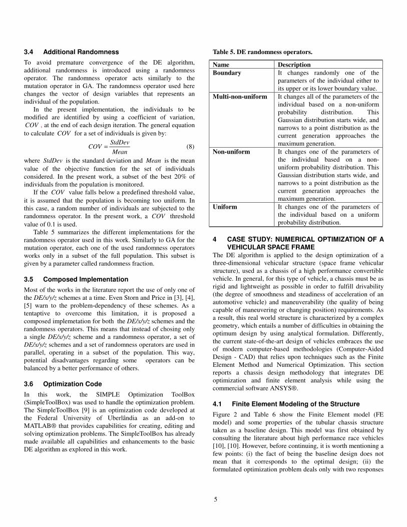
3.4 Additional Randomness

To avoid premature convergence of the DE algorithm,

additional randomness is introduced using a randomness

operator. The randomness operator acts similarly to the

mutation operator in GA. The randomness operator used here

changes the vector of design variables that represents an

individual of the population.

In the present implementation, the individuals to be

modified are identified by using a coefficient of variation,

COV , at the end of each design iteration. The general equation

to calculate COV for a set of individuals is given by:

StdDev

COVMean

= (8)

where StdDev is the standard deviation and Mean is the mean

value of the objective function for the set of individuals

considered. In the present work, a subset of the best 20% of

individuals from the population is monitored.

If the COV value falls below a predefined threshold value,

it is assumed that the population is becoming too uniform. In

this case, a random number of individuals are subjected to the

randomness operator. In the present work, a COV threshold

value of 0.1 is used.

Table 5 summarizes the different implementations for the

randomness operator used in this work. Similarly to GA for the

mutation operator, each one of the used randomness operators

works only in a subset of the full population. This subset is

given by a parameter called randomness fraction.

3.5 Composed Implementation

Most of the works in the literature report the use of only one of

the DE/x/y/z schemes at a time. Even Storn and Price in [3], [4],

[5] warn to the problem-dependency of these schemes. As a

tentaptive to overcome this limitation, it is proposed a

composed implemetation for both the DE/x/y/z schemes and the

randomness operators. This means that instead of chosing only

a single DE/x/y/z scheme and a randomness operator, a set of

DE/x/y/z schemes and a set of randomness operators are used in

parallel, operating in a subset of the population. This way,

potential disadvantages regarding some operators can be

balanced by a better performance of others.

3.6 Optimization Code

In this work, the SIMPLE Optimization ToolBox

(SimpleToolBox) was used to handle the optimization problem.

The SimpleToolBox [9] is an optimization code developed at

the Federal University of Uberlândia as an add-on to

MATLAB® that provides capabilities for creating, editing and

solving optimization problems. The SimpleToolBox has already

made available all capabilities and enhancements to the basic

DE algorithm as explored in this work.

Table 5. DE randomness operators.

Name Description

Boundary It changes randomly one of the

parameters of the individual either to

its upper or its lower boundary value.

Multi-non-uniform It changes all of the parameters of the

individual based on a non-uniform

probability distribution. This

Gaussian distribution starts wide, and

narrows to a point distribution as the

current generation approaches the

maximum generation.

Non-uniform It changes one of the parameters of

the individual based on a non-

uniform probability distribution. This

Gaussian distribution starts wide, and

narrows to a point distribution as the

current generation approaches the

maximum generation.

Uniform It changes one of the parameters of

the individual based on a uniform

probability distribution.

4 CASE STUDY: NUMERICAL OPTIMIZATION OF A VEHICULAR SPACE FRAME

The DE algorithm is applied to the design optimization of a

three-dimensional vehicular structure (space frame vehicular

structure), used as a chassis of a high performance convertible

vehicle. In general, for this type of vehicle, a chassis must be as

rigid and lightweight as possible in order to fulfill drivability

(the degree of smoothness and steadiness of acceleration of an

automotive vehicle) and maneuverability (the quality of being

capable of maneuvering or changing position) requirements. As

a result, this real world structure is characterized by a complex

geometry, which entails a number of difficulties in obtaining the

optimum design by using analytical formulation. Differently,

the current state-of-the-art design of vehicles embraces the use

of modern computer-based methodologies (Computer-Aided

Design - CAD) that relies upon techniques such as the Finite

Element Method and Numerical Optimization. This section

reports a chassis design methodology that integrates DE

optimization and finite element analysis while using the

commercial software ANSYS®.

4.1 Finite Element Modeling of the Structure

Figure 2 and Table 6 show the Finite Element model (FE

model) and some properties of the tubular chassis structure

taken as a baseline design. This model was first obtained by

consulting the literature about high performance race vehicles

[10], [10]. However, before continuing, it is worth mentioning a

few points: (i) the fact of being the baseline design does not

mean that it corresponds to the optimal design; (ii) the

formulated optimization problem deals only with two responses

6

(mass and torsional stiffness). In a more realistic scenario, it

would be necessary to include other factors such as dynamic

responses, manufacture constraints, etc. In this specific paper,

the focus is on the capability of DE in handling mechanical

engineering problems, exemplified as the standard structural

optimization problem of mass reduction (vehicular frame

structure), while increasing the stiffness.

Figure 2. Baseline for the vehicular space frame structure.

4.2 Optimization Problem Formulation

According to the literature [10],[10],[12], for design purposes

the most effective strategy should consider both the mass

reduction and the increase of the torsional stiffness.

Vanderplaats [13] literally affirms that “for automobiles, a ten

percent mass reduction will increase fuel economy by about

seven percent. Only a one percent economy improvement will

save nearly three billion dollars per year in the U.S. at the

pump”. On the other hand, torsional stiffness is related to the

drivability and maneuverability [10], [10].

Considering the present case study, the geometry of both the

front side and the back side of the structure can not be changed,

since they are designed to receive other elements such as

engine, fuel tank, etc. Thus, to achieve the design goals, the

central part of the structure, the thickness and the external

diameter of the tubes are assumed as design variables.

Regarding the central part of the chassis, a total number of

31 nodal coordinates are assumed as continuous variables. The

bounds for these variables are defined as an interval for which

the center is taken from the baseline design. In the present

work, the bounds range from 0.75 to 1.25 of the baseline

value. It means that the baseline design is placed at the center of

the design space and each node can be shifted to a position that

has coordinates varying from 75% to 125% of the baseline

counterparts. About the tube, the external diameter is a discrete

variable that can assume one of the values shown in Table 7.

For all these diameter values, the thickness ranges from 31.06 10 m

−× to 33.00 10 m−× . It is worth mentioning that these

values were obtained from commercial steel tubes found in the

market. This way, the optimization is defined as a problem of

32 design variables (31 continuous and 1 discrete).

Table 6. Properties of the baseline model.

Element type NDOF per

element

NDOF of the

model FE

model BEAM04 12 18675

Young’s

modulus 2

N m Poisson ratio

Density 3

Kg m Material

112.1 10× 0.3 7850

Mass

[ ]Kg

Torsional stiffness

[ ]degKgf m⋅ General

139.52 1,728.1

Table 7. External diameter.

Design variable

values 1 2 3 4 5

Corresponding

diameter

310 m

− ×

38.10

41.27

44.45

47.60

50.80

Then, in order to explore the capabilities of the DE

algorithm to handle both multi-objective and constrained

optimization problems, four formulations for the optimization

problem were tested. The first one takes both mass and stiffness

requirements as constraints of the design and using the facilities

of the “Classical Exterior Penalty Function”. The optimization

problem is defined as the minimization of a dummy objective

function given by:

( ) 0F =x (9)

subject to:

( )

( )

1

max

2

min

Mass constraint: 1.0 0

Stiffness constraint: 1.0 0

MassG

M

KG

K

= − ≤

= − ≤

x

x

(10)

The second formulation takes the mass reduction as

objective and makes the stiffness requirement as a constraint

function. The optimization problem is defined as the

minimization of the objective function given by:

( )max

Mass objective:Mass

FM

=x (11)

7

subject to:

( )min

Stiffness constraint: 1.0 0K

GK

= − ≤x (12)

The third formulation takes the stiffness increasing as

objective and makes the mass reduction as a constraint function.

The optimization problem is defined as the minimization of the

objective function given by:

( )min

Stiffness objective:K

FK

= −x (13)

subject to:

( )max

Mass constraint: 1.0 0Mass

GM

= − ≤x (14)

Finally, the fourth formulation takes both the mass reduction

and the stiffness increasing as objectives to build a multi-

objective problem to be solved by using the “Weighted Min-

Max Method”:

( )( )( )

1

2

=F

F

xF x

x (15)

where:

( )

( )

1

max

2

min

Mass objective:

Stiffness objective:

MassF

M

KF

K

=

= −

x

x

(16)

For all the previously presented formulations, max

100 [ ]M Kg=

and [ ]min2,500 degK Kgf m= ⋅ are given. These values have

two main purposes: (i) normalization (scaling) of the responses,

since the magnitudes of the mass and the torsional stiffness are

quite different; and (ii) mainly in the constrained formulation,

they behave like limit values for the responses.

5 RESULTS Table 8 shows the setup for the DE algorithm used for all

formulations studied. As can be observed, the population size is

only 3.125 times the number of design variables. This is much

smaller than the suggested value of 10 times the number of

design variables. However, since a FE analysis is required

during the evaluation of the objective function, a reduced

number of function evaluations appear as one of the

requirements for this optimization problem. Thus, the

enhancements in the basic DE algorithm play an important role

in the success of the optimization task. In this sense, the total

number of function evaluations, i.e. 5000, is divided in such a

way that the DE dynamics can be fully explored. In other

words, the set of parameters must allow for both global and

local searches. One way to see how this can be achieved is

through the contrast between the population size and the

number of iterations. Small number of iterations means short

global and local exploration phases and one way to improve the

algorithm’s performance under these conditions is using a larger

set of points. In the present work, the balance is achieved by

using the parameters shown in Tab. 8.

Table 8. DE parameters setup.

Population

size Iterations

Amplification

factor (F)

Crossover

probability

(CR)

100 50 0.8 0.5

DE strategies

DE randomness

operators (randomness

fraction of 5%)

DE/rand/1/exp,

DE/rand/2/exp,

DE/best/2/exp,

DE/rand-to-best/1/exp

Boundary

Multi-non-uniform

Non-uniform

Uniform

Table 9 illustrates the final results obtained regarding the four

different problem formulations (as presented in the previous

section). In general, it can be observed that all cases show some

improvement for the values of both the mass and the torsional

stiffness as compared with the original baseline design.

Analyzing only the final mass value, it is hard to decide which

design is the best. However, by also considering the torsional

stiffness value, the result found for formulation #3 seems to be

slightly better from a compromise solution point of view. Figure

3 shows how the final design looks like in this case. As

explained before, in this case only the total mass and the

torsional stiffness were considered. In a more realistic picture

other responses of interest could make the task more difficult

and probably the results would not be as good as the above

presented.

Table 9. Design optimization results.

Mass Torsional stiffness

Formulation Value

[ ]Kg % of

reduction

Value

[ ]degKgf m⋅

% of

increasing

#1 107.51 22.9429 2,484.2 43.7533

#2 115.32 17.3452 2,493.3 44.2798

#3 106.83 23.4303 2,856.3 65.2856

#4 106.53 23.6454 2,242.1 29.7436

Baseline 139.52 1,728.1

8

Figure 3. Final design obtained by using formulation #3.

Figure 4 shows the DE performance along the iterations of

the optimization task. Figure 4-(a) illustrates the range of the

objective function value; it can be observed that during the first

iterations the exploring optimization process is more global

than local, which reflects at the end of the optimization task.

Figure 4-(b) gives the histogram of the objective function

values for the final population; if compared with the range of

the initial population, it can be seen that the population

converged to a smaller region of the design space. Figure 4-(c)

shows the evolution of the COV over the iterations; it is

possible to notice that the subset of the population behaves

more uniformly than the full population itself. Finally, Figure 4-

(d) illustrates how the stopping criteria evolve during the

optimization task.

As a way to assess the efficiency of DE in accomplishing the

optimization, the results obtained for formulation #3 are

compared with the results obtained through a hybrid cascade-

type scheme by using a population-based algorithm for global

search and a point-based algorithm for local search. More

specifically, the global search is performed by three different

algorithms, namely ACO, GA and PSO. The local search is

performed by a Nelder-Mead simplex direct search algorithm

(fminsearch MATLAB function). Since ACO, GA and PSO are

used only for global search, both the population size and the

number of iterations are set as 50. It is worth mentioning that at

the local search phase only continuous variables are

manipulated by fminsearch. In summary, this setup for the

optimization has two aims: (i) take advantage of the strong

points of each algorithm, and (ii) keep the number of function

evaluations as low as possible.

Table 10 shows the results obtained. It can be seen that even

when the hybrid schemes were more efficient in reducing the

mass, they were not efficient in the improvement of the

torsional stiffness.

Table 10. DE versus hybrid schemes.

Mass Torsional stiffness

Formulation Value

[ ]Kg % of

reduction

Value

[ ]degKgf m⋅

% of

increasing

DE 106.83 23.4303 2,856.3 65.2856

ACO +

fminsearch 100 28.3257 1765.08 2.1399

GA +

fminsearch 100.03 28.3042 1809.56 4.7138

PSO +

fminsearch 108.55 22.1975 1933.4 11.8801

Baseline 139.52 1,728.1

6 CONCLUSIONS AND FUTURE WORK

The present contribution demonstrated the application of

Differential Evolution to solve a realistic design optimization

test problem. Improvements were implemented in the original

basic algorithm. The selected case study was a three-

dimensional vehicular structure optimization problem modeled

using the commercial Finite Element software ANSYS® . A

combination of continuous and discrete design variables was

successfully handled by the algorithm. It is also important to say

that the algorithm used was able to handle constraint functions

and performed satisfactorily in the context of multicriteria

optimization design. Finally, a comparison with hybrid schemes

encourages the authors in the sense of exploring the DE

capabilities for global and local searches in the optimal design

of mechanical systems.

9

(a) Objective range. (b) Objective diversity of the final population.

(c) Coefficient of variation (COV). (c) Stop criteria.

Figure 4. DE performance.

7 ACKNOWLEDGEMENTS

Mr. Felipe Viana and Mr. Fernando Oliveira are both thankful

to CNPq Brazilian Research Agency for their PhD and Master

scholarships, respectively. Dr. Valder Steffen acknowledges

CNPq for the partial financing of the present work (Proc.

470346/2006-0).

8 REFERENCES

[1] Venter, G. and Sobieski, J. S., 2002, Particle Swarm

ptimization, Proceedings of the 43rd

AIAA/ASME/ASCE/AHS/ASC Structures, Structural

Dynamics, and Materials Conference, Denver, USA.

[2] Viana, F. A. C. and Steffen Jr, V., 2005, Natural Methods

Applied to Direct and Inverse Problems. In Balthazar, J.

M., Brasil, R. M. L. R. F., Macau, E. E. N. and Pontes, B.

R., eds, Proceedings of the Workshop on Nonlinear

Phenomena Modeling and Their Applications, Rio Claro,

Brazil.

[3] Storn, R. and Price, K., Differential Evolution - a simple

and efficient adaptive scheme for global optimization over

continuous spaces. Technical Report TR-95-012,

International Computer Science Institute, Berkley, March

1995.

[4] Storn, R. and Price, K., Differential Evolution - A Simple

and Efficient Heuristic for Global optimization over

Continuous Spaces. Journal of Global Optimization,

11:341–359, 1997.

[5] Storn, R., On the Usage of Differential Evolution for

Function Optimization. In 1996 Biennial Conference of

the North American Fuzzy Information Processing

Society, Berkeley, USA, pages 519–523, June 19-22

1996.

[6] Marler, R. T. and Arora, J. S., Survey of Multi-Objective

Optimization Methods for Engineering. Structural and

Multidisciplinary Otpimization, 26:369–395, 2004.

[7] Michalewicz, Z., Genetic Algorithms, Numerical

Optimization and Constraints. In Proceedings of the 6th

International Conference on Genetic Algorithms,

Pittsburgh, pages 151–158, July 15-19, 1995.

10

[8] Coello, C. A. C., Theoretical and Numerical Constraint-

Handling Techniques used in Evolutionary Algorithms: a

Survey of the State of the Art. Computer Methods in

Applied Mechanics and Engineering, Volume 191, Issues

11-12, pp 1245-1287, 2002.

[9] Viana, F. A. C. and Steffen Jr, V., "SIMPLE Optimization

ToolBox - Users Guide," 2th edition,

http://www.geocities.com/fchegury/, [downloaded at

November 2006].

[10] Tompson, L.L.; Raju, S.; Law, E.H.; 1998; “Design of a

Winston Cup Chassis for Torsional Stiffness”; SAE

Technical Paper Series No. 983053 – Motorsports

Engineering Conference Proceedings Volume 1: Vehicle

Design and Safety; Dearborn, Michigan, USA.

[11] Aird, F.; “Race Car Chassis Design and Construction”;

MBI Publishing Company; 1997.

[12] Happian, J.S.; 2002; “An Introduction to Modern Vehicle

Design”; ISBN 0 7680 0596 5 ON –R-295; Society of

Automotive Engineers, Inc.; Reed Educational and

Professional Publishing.

[13] Vanderplaats, G. N.; “Structural Optimization for statics,

dynamics and beyond”. In XI DINAME - International

Symposium on Dynamic Problems of Mechanics, Ouro

Preto, Brazil, February 28 - March 04, 2005.