Differential Equations, Dynamical Systems, and an Introduction to ...
432
Transcript of Differential Equations, Dynamical Systems, and an Introduction to ...


DIFFERENTIAL EQUATIONS,
DYNAMICAL SYSTEMS, AND
AN INTRODUCTION
TO CHAOS

This is volume 60, 2ed in the PURE AND APPLIED MATHEMATICS SeriesFounding Editors: Paul A. Smith and Samuel Eilenberg

DIFFERENTIAL EQUATIONS,
DYNAMICAL SYSTEMS, AND
AN INTRODUCTION
TO CHAOS
Morris W. HirschUniversity of California, Berkeley
Stephen SmaleUniversity of California, Berkeley
Robert L. DevaneyBoston University
Amsterdam Boston Heidelberg London New York Oxford
Paris San Diego San Francisco Singapore Sydney Tokyo
Academic Press is an imprint of Elsevier

Senior Editor, Mathematics Barbara HollandAssociate Editor Tom SingerProject Manager Kyle SarofeenMarketing Manager Linda BeattieProduction Services Beth Callaway, Graphic WorldCover Design Eric DeCiccoCopyediting Graphic WorldComposition Cepha Imaging Pvt. Ltd.Printer Maple-Vail
This book is printed on acid-free paper.
Copyright 2004, Elsevier (USA)
All rights reserved.No part of this publication may be reproduced or transmitted in any form or by any means,electronic or mechanical, including photocopy, recording, or any information storage andretrieval system, without permission in writing from the publisher.
Permissions may be sought directly from Elsevier’s Science & Technology RightsDepartment in Oxford, UK: phone: (+44) 1865 843830, fax: (+44) 1865 853333, e-mail:[email protected]. You may also complete your request on-line via the ElsevierScience homepage (http://elsevier.com), by selecting “Customer Support” and then“Obtaining Permissions.”
Academic PressAn imprint of Elsevier525 B Street, Suite 1900, San Diego, California 92101-4495, USAhttp://www.academicpress.com
Academic PressAn imprint of Elsevier84 Theobald’s Road, London WC1X 8RR, UKhttp://www.academicpress.com
Library of Congress Cataloging-in-Publication Data
Hirsch, Morris W., 1933-Differential equations, dynamical systems, and an introduction to chaos/Morris W.
Hirsch, Stephen Smale, Robert L. Devaney.p. cm.
Rev. ed. of: Differential equations, dynamical systems, and linear algebra/Morris W.Hirsch and Stephen Smale. 1974.Includes bibliographical references and index.ISBN 0-12-349703-5 (alk. paper)1. Differential equations. 2. Algebras, Linear. 3. Chaotic behavior in systems. I. Smale,
Stephen, 1930- II. Devaney, Robert L., 1948- III. Hirsch, Morris W., 1933-Differential Equations, dynamical systems, and linear algebra. IV. Title.
QA372.H67 2003515’.35--dc22
2003058255
PRINTED IN THE UNITED STATES OF AMERICA03 04 05 06 07 08 9 8 7 6 5 4 3 2 1
Contents
Preface x
CHAPTER 1 First-Order Equations 1
1.1 The Simplest Example 1
1.2 The Logistic Population Model 4
1.3 Constant Harvesting and Bifurcations 7
1.4 Periodic Harvesting and Periodic
Solutions 9
1.5 Computing the Poincaré Map 12
1.6 Exploration: A Two-Parameter Family 15
CHAPTER 2 Planar Linear Systems 21
2.1 Second-Order Differential Equations 23
2.2 Planar Systems 24
2.3 Preliminaries from Algebra 26
2.4 Planar Linear Systems 29
2.5 Eigenvalues and Eigenvectors 30
2.6 Solving Linear Systems 33
2.7 The Linearity Principle 36
CHAPTER 3 Phase Portraits for Planar Systems 39
3.1 Real Distinct Eigenvalues 39
3.2 Complex Eigenvalues 44
v

vi Contents
3.3 Repeated Eigenvalues 47
3.4 Changing Coordinates 49
CHAPTER 4 Classification of Planar Systems 61
4.1 The Trace-Determinant Plane 61
4.2 Dynamical Classification 64
4.3 Exploration: A 3D Parameter Space 71
CHAPTER 5 Higher Dimensional Linear Algebra 75
5.1 Preliminaries from Linear Algebra 75
5.2 Eigenvalues and Eigenvectors 83
5.3 Complex Eigenvalues 86
5.4 Bases and Subspaces 89
5.5 Repeated Eigenvalues 95
5.6 Genericity 101
CHAPTER 6 Higher Dimensional Linear Systems 107
6.1 Distinct Eigenvalues 107
6.2 Harmonic Oscillators 114
6.3 Repeated Eigenvalues 119
6.4 The Exponential of a Matrix 123
6.5 Nonautonomous Linear Systems 130
CHAPTER 7 Nonlinear Systems 139
7.1 Dynamical Systems 140
7.2 The Existence and Uniqueness
Theorem 142
7.3 Continuous Dependence of Solutions 147
7.4 The Variational Equation 149
7.5 Exploration: Numerical Methods 153
CHAPTER 8 Equilibria in Nonlinear Systems 159
8.1 Some Illustrative Examples 159
8.2 Nonlinear Sinks and Sources 165
8.3 Saddles 168
8.4 Stability 174
8.5 Bifurcations 176
8.6 Exploration: Complex Vector Fields 182

Contents vii
CHAPTER 9 Global Nonlinear Techniques 189
9.1 Nullclines 189
9.2 Stability of Equilibria 194
9.3 Gradient Systems 203
9.4 Hamiltonian Systems 207
9.5 Exploration: The Pendulum with Constant
Forcing 210
CHAPTER 10 Closed Orbits and Limit Sets 215
10.1 Limit Sets 215
10.2 Local Sections and Flow Boxes 218
10.3 The Poincaré Map 220
10.4 Monotone Sequences in Planar Dynamical
Systems 222
10.5 The Poincaré-Bendixson Theorem 225
10.6 Applications of Poincaré-Bendixson 227
10.7 Exploration: Chemical Reactions That
Oscillate 230
CHAPTER 11 Applications in Biology 235
11.1 Infectious Diseases 235
11.2 Predator/Prey Systems 239
11.3 Competitive Species 246
11.4 Exploration: Competition and
Harvesting 252
CHAPTER 12 Applications in Circuit Theory 257
12.1 An RLC Circuit 257
12.2 The Lienard Equation 261
12.3 The van der Pol Equation 262
12.4 A Hopf Bifurcation 270
12.5 Exploration: Neurodynamics 272
CHAPTER 13 Applications in Mechanics 277
13.1 Newton’s Second Law 277
13.2 Conservative Systems 280
13.3 Central Force Fields 281
13.4 The Newtonian Central Force
System 285

viii Contents
13.5 Kepler’s First Law 289
13.6 The Two-Body Problem 292
13.7 Blowing Up the Singularity 293
13.8 Exploration: Other Central Force
Problems 297
13.9 Exploration: Classical Limits of Quantum
Mechanical Systems 298
CHAPTER 14 The Lorenz System 303
14.1 Introduction to the Lorenz System 304
14.2 Elementary Properties of the Lorenz
System 306
14.3 The Lorenz Attractor 310
14.4 A Model for the Lorenz Attractor 314
14.5 The Chaotic Attractor 319
14.6 Exploration: The Rössler Attractor 324
CHAPTER 15 Discrete Dynamical Systems 327
15.1 Introduction to Discrete Dynamical
Systems 327
15.2 Bifurcations 332
15.3 The Discrete Logistic Model 335
15.4 Chaos 337
15.5 Symbolic Dynamics 342
15.6 The Shift Map 347
15.7 The Cantor Middle-Thirds Set 349
15.8 Exploration: Cubic Chaos 352
15.9 Exploration: The Orbit Diagram 353
CHAPTER 16 Homoclinic Phenomena 359
16.1 The Shil’nikov System 359
16.2 The Horseshoe Map 366
16.3 The Double Scroll Attractor 372
16.4 Homoclinic Bifurcations 375
16.5 Exploration: The Chua Circuit 379
CHAPTER 17 Existence and Uniqueness Revisited 383
17.1 The Existence and Uniqueness
Theorem 383
17.2 Proof of Existence and Uniqueness 385

Contents ix
17.3 Continuous Dependence on Initial
Conditions 392
17.4 Extending Solutions 395
17.5 Nonautonomous Systems 398
17.6 Differentiability of the Flow 400
Bibliography 407
Index 411
Preface
In the 30 years since the publication of the first edition of this book, muchhas changed in the field of mathematics known as dynamical systems. In theearly 1970s, we had very little access to high-speed computers and computergraphics. The word chaos had never been used in a mathematical setting, andmost of the interest in the theory of differential equations and dynamicalsystems was confined to a relatively small group of mathematicians.
Things have changed dramatically in the ensuing 3 decades. Computers areeverywhere, and software packages that can be used to approximate solutionsof differential equations and view the results graphically are widely available.As a consequence, the analysis of nonlinear systems of differential equationsis much more accessible than it once was. The discovery of such compli-cated dynamical systems as the horseshoe map, homoclinic tangles, and theLorenz system, and their mathematical analyses, convinced scientists that sim-ple stable motions such as equilibria or periodic solutions were not always themost important behavior of solutions of differential equations. The beautyand relative accessibility of these chaotic phenomena motivated scientists andengineers in many disciplines to look more carefully at the important differen-tial equations in their own fields. In many cases, they found chaotic behavior inthese systems as well. Now dynamical systems phenomena appear in virtuallyevery area of science, from the oscillating Belousov-Zhabotinsky reaction inchemistry to the chaotic Chua circuit in electrical engineering, from compli-cated motions in celestial mechanics to the bifurcations arising in ecologicalsystems.
As a consequence, the audience for a text on differential equations anddynamical systems is considerably larger and more diverse than it was in
x

Preface xi
the 1970s. We have accordingly made several major structural changes tothis text, including the following:
1. The treatment of linear algebra has been scaled back. We have dispensedwith the generalities involved with abstract vector spaces and normedlinear spaces. We no longer include a complete proof of the reductionof all n × n matrices to canonical form. Rather we deal primarily withmatrices no larger than 4 × 4.
2. We have included a detailed discussion of the chaotic behavior in theLorenz attractor, the Shil’nikov system, and the double scroll attractor.
3. Many new applications are included; previous applications have beenupdated.
4. There are now several chapters dealing with discrete dynamical systems.5. We deal primarily with systems that are C∞, thereby simplifying many of
the hypotheses of theorems.
The book consists of three main parts. The first part deals with linear systemsof differential equations together with some first-order nonlinear equations.The second part of the book is the main part of the text: Here we concentrate onnonlinear systems, primarily two dimensional, as well as applications of thesesystems in a wide variety of fields. The third part deals with higher dimensionalsystems. Here we emphasize the types of chaotic behavior that do not occur inplanar systems, as well as the principal means of studying such behavior, thereduction to a discrete dynamical system.
Writing a book for a diverse audience whose backgrounds vary greatly posesa significant challenge. We view this book as a text for a second course indifferential equations that is aimed not only at mathematicians, but also atscientists and engineers who are seeking to develop sufficient mathematicalskills to analyze the types of differential equations that arise in their disciplines.Many who come to this book will have strong backgrounds in linear algebraand real analysis, but others will have less exposure to these fields. To makethis text accessible to both groups, we begin with a fairly gentle introductionto low-dimensional systems of differential equations. Much of this will be areview for readers with deeper backgrounds in differential equations, so weintersperse some new topics throughout the early part of the book for thesereaders.
For example, the first chapter deals with first-order equations. We beginthis chapter with a discussion of linear differential equations and the logisticpopulation model, topics that should be familiar to anyone who has a rudimen-tary acquaintance with differential equations. Beyond this review, we discussthe logistic model with harvesting, both constant and periodic. This allowsus to introduce bifurcations at an early stage as well as to describe Poincarémaps and periodic solutions. These are topics that are not usually found inelementary differential equations courses, yet they are accessible to anyone

xii Preface
with a background in multivariable calculus. Of course, readers with a limitedbackground may wish to skip these specialized topics at first and concentrateon the more elementary material.
Chapters 2 through 6 deal with linear systems of differential equations.Again we begin slowly, with Chapters 2 and 3 dealing only with planar sys-tems of differential equations and two-dimensional linear algebra. Chapters5 and 6 introduce higher dimensional linear systems; however, our empha-sis remains on three- and four-dimensional systems rather than completelygeneral n-dimensional systems, though many of the techniques we describeextend easily to higher dimensions.
The core of the book lies in the second part. Here we turn our atten-tion to nonlinear systems. Unlike linear systems, nonlinear systems presentsome serious theoretical difficulties such as existence and uniqueness of solu-tions, dependence of solutions on initial conditions and parameters, and thelike. Rather than plunge immediately into these difficult theoretical questions,which require a solid background in real analysis, we simply state the impor-tant results in Chapter 7 and present a collection of examples that illustratewhat these theorems say (and do not say). Proofs of all of these results areincluded in the final chapter of the book.
In the first few chapters in the nonlinear part of the book, we introducesuch important techniques as linearization near equilibria, nullcline analysis,stability properties, limit sets, and bifurcation theory. In the latter half of thispart, we apply these ideas to a variety of systems that arise in biology, electricalengineering, mechanics, and other fields.
Many of the chapters conclude with a section called “Exploration.” Thesesections consist of a series of questions and numerical investigations dealingwith a particular topic or application relevant to the preceding material. Ineach Exploration we give a brief introduction to the topic at hand and providereferences for further reading about this subject. But we leave it to the reader totackle the behavior of the resulting system using the material presented earlier.We often provide a series of introductory problems as well as hints as to howto proceed, but in many cases, a full analysis of the system could become amajor research project. You will not find “answers in the back of the book” forthese questions; in many cases nobody knows the complete answer. (Except,of course, you!)
The final part of the book is devoted to the complicated nonlinear behaviorof higher dimensional systems known as chaotic behavior. We introduce theseideas via the famous Lorenz system of differential equations. As is often thecase in dimensions three and higher, we reduce the problem of comprehendingthe complicated behavior of this differential equation to that of understandingthe dynamics of a discrete dynamical system or iterated function. So we thentake a detour into the world of discrete systems, discussing along the way howsymbolic dynamics may be used to describe completely certain chaotic systems.

Preface xiii
We then return to nonlinear differential equations to apply these techniquesto other chaotic systems, including those that arise when homoclinic orbitsare present.
We maintain a website at math.bu.edu/hsd devoted to issues regard-ing this text. Look here for errata, suggestions, and other topics of interest toteachers and students of differential equations. We welcome any contributionsfrom readers at this site.
It is a special pleasure to thank Bard Ermentrout, John Guckenheimer, TassoKaper, Jerrold Marsden, and Gareth Roberts for their many fine commentsabout an earlier version of this edition. Thanks are especially due to DanielLook and Richard Moeckel for a careful reading of the entire manuscript.Many of the phase plane drawings in this book were made using the excellentMathematica package called DynPac: A Dynamical Systems Package for Math-ematica written by Al Clark. See www.me.rochester.edu/˜clark/dynpac.html.And, as always, Ki��er Devaney digested the entire manuscript; all errors thatremain are due to her.

Acknowledgements
I would like to thank the following reviewers:
Bruce Peckham, University of MinnesotaBard Ermentrout, University of PittsburghRichard Moeckel, University of MinnesotaJerry Marsden, CalTechJohn Guckenheimer, Cornell UniversityGareth Roberts, College of Holy CrossRick Moeckel, University of MinnesotaHans Lindblad, University of California San DiegoTom LoFaro, Gustavus Adolphus CollegeDaniel M. Look, Boston University
xiv

1First-Order Equations
The purpose of this chapter is to develop some elementary yet importantexamples of first-order differential equations. These examples illustrate someof the basic ideas in the theory of ordinary differential equations in the simplestpossible setting.
We anticipate that the first few examples in this chapter will be familiar toreaders who have taken an introductory course in differential equations. Laterexamples, such as the logistic model with harvesting, are included to give thereader a taste of certain topics (bifurcations, periodic solutions, and Poincarémaps) that we will return to often throughout this book. In later chapters, ourtreatment of these topics will be much more systematic.
1.1 The Simplest Example
The differential equation familiar to all calculus students
dx
dt= ax
is the simplest differential equation. It is also one of the most important.First, what does it mean? Here x = x(t ) is an unknown real-valued functionof a real variable t and dx/dt is its derivative (we will also use x ′ or x ′(t )for the derivative). Also, a is a parameter; for each value of a we have a
1

2 Chapter 1 First-Order Equations
different differential equation. The equation tells us that for every value of tthe relationship
x ′(t ) = ax(t )
is true.The solutions of this equation are obtained from calculus: If k is any real
number, then the function x(t ) = keat is a solution since
x ′(t ) = akeat = ax(t ).
Moreover, there are no other solutions. To see this, let u(t ) be any solution andcompute the derivative of u(t )e−at :
d
dt
(u(t )e−at ) = u′(t )e−at + u(t )(−ae−at )
= au(t )e−at − au(t )e−at = 0.
Therefore u(t )e−at is a constant k, so u(t ) = keat . This proves our assertion.We have therefore found all possible solutions of this differential equation. Wecall the collection of all solutions of a differential equation the general solutionof the equation.
The constant k appearing in this solution is completely determined if thevalue u0 of a solution at a single point t0 is specified. Suppose that a functionx(t ) satisfying the differential equation is also required to satisfy x(t0) = u0.Then we must have keat0 = u0, so that k = u0e−at0 . Thus we have determinedk, and this equation therefore has a unique solution satisfying the specifiedinitial condition x(t0) = u0. For simplicity, we often take t0 = 0; then k = u0.There is no loss of generality in taking t0 = 0, for if u(t ) is a solution withu(0) = u0, then the function v(t ) = u(t − t0) is a solution with v(t0) = u0.
It is common to restate this in the form of an initial value problem:
x ′ = ax , x(0) = u0.
A solution x(t ) of an initial value problem must not only solve the differentialequation, but it must also take on the prescribed initial value u0 at t = 0.
Note that there is a special solution of this differential equation when k = 0.This is the constant solution x(t ) ≡ 0. A constant solution such as this is calledan equilibrium solution or equilibrium point for the equation. Equilibria areoften among the most important solutions of differential equations.
The constant a in the equation x ′ = ax can be considered a parameter.If a changes, the equation changes and so do the solutions. Can we describe

1.1 The Simplest Example 3
qualitatively the way the solutions change? The sign of a is crucial here:
1. If a > 0, limt→∞keat equals ∞ when k > 0, and equals −∞ when k < 0;2. If a = 0, keat = constant;3. If a < 0, limt→∞keat = 0.
The qualitative behavior of solutions is vividly illustrated by sketching thegraphs of solutions as in Figure 1.1. Note that the behavior of solutions is quitedifferent when a is positive and negative. When a > 0, all nonzero solutionstend away from the equilibrium point at 0 as t increases, whereas when a < 0,solutions tend toward the equilibrium point. We say that the equilibrium pointis a source when nearby solutions tend away from it. The equilibrium point isa sink when nearby solutions tend toward it.
We also describe solutions by drawing them on the phase line. Because thesolution x(t ) is a function of time, we may view x(t ) as a particle moving alongthe real line. At the equilibrium point, the particle remains at rest (indicated
x
t
Figure 1.1 The solution graphs and phaseline for x ′ = ax for a > 0. Each graphrepresents a particular solution.
t
x
Figure 1.2 The solution graphs andphase line for x ′ = ax for a < 0.

4 Chapter 1 First-Order Equations
by a solid dot), while any other solution moves up or down the x-axis, asindicated by the arrows in Figure 1.1.
The equation x ′ = ax is stable in a certain sense if a �= 0. More precisely,if a is replaced by another constant b whose sign is the same as a, then thequalitative behavior of the solutions does not change. But if a = 0, the slightestchange in a leads to a radical change in the behavior of solutions. We thereforesay that we have a bifurcation at a = 0 in the one-parameter family of equationsx ′ = ax .
1.2 The Logistic Population Model
The differential equation x ′ = ax above can be considered a simplistic modelof population growth when a > 0. The quantity x(t ) measures the populationof some species at time t . The assumption that leads to the differential equa-tion is that the rate of growth of the population (namely, dx/dt ) is directlyproportional to the size of the population. Of course, this naive assumptionomits many circumstances that govern actual population growth, including,for example, the fact that actual populations cannot increase with bound.
To take this restriction into account, we can make the following furtherassumptions about the population model:
1. If the population is small, the growth rate is nearly directly proportionalto the size of the population;
2. but if the population grows too large, the growth rate becomes negative.
One differential equation that satisfies these assumptions is the logisticpopulation growth model. This differential equation is
x ′ = ax(1 − x
N
).
Here a and N are positive parameters: a gives the rate of population growthwhen x is small, while N represents a sort of “ideal” population or “carryingcapacity.” Note that if x is small, the differential equation is essentially x ′ = ax[since the term 1 − (x/N ) ≈ 1], but if x > N , then x ′ < 0. Thus this simpleequation satisfies the above assumptions. We should add here that there aremany other differential equations that correspond to these assumptions; ourchoice is perhaps the simplest.
Without loss of generality we will assume that N = 1. That is, we willchoose units so that the carrying capacity is exactly 1 unit of population, andx(t ) therefore represents the fraction of the ideal population present at time t .

1.2 The Logistic Population Model 5
Therefore the logistic equation reduces to
x ′ = fa(x) = ax(1 − x).
This is an example of a first-order, autonomous, nonlinear differential equa-tion. It is first order since only the first derivative of x appears in the equation.It is autonomous since the right-hand side of the equation depends on x alone,not on time t . And it is nonlinear since fa(x) is a nonlinear function of x . Theprevious example, x ′ = ax , is a first-order, autonomous, linear differentialequation.
The solution of the logistic differential equation is easily found by the tried-and-true calculus method of separation and integration:∫
dx
x(1 − x)=
∫a dt .
The method of partial fractions allows us to rewrite the left integral as∫ (1
x+ 1
1 − x
)dx .
Integrating both sides and then solving for x yields
x(t ) = Keat
1 + Keat
where K is the arbitrary constant that arises from integration. Evaluating thisexpression at t = 0 and solving for K gives
K = x(0)
1 − x(0).
Using this, we may rewrite this solution as
x(0)eat
1 − x(0) + x(0)eat.
So this solution is valid for any initial population x(0). When x(0) = 1,we have an equilibrium solution, since x(t ) reduces to x(t ) ≡ 1. Similarly,x(t ) ≡ 0 is also an equilibrium solution.
Thus we have “existence” of solutions for the logistic differential equation.We have no guarantee that these are all of the solutions to this equation at thisstage; we will return to this issue when we discuss the existence and uniquenessproblem for differential equations in Chapter 7.

6 Chapter 1 First-Order Equations
x
t
x�1
x�0
Figure 1.3 The slope field, solution graphs, and phase line forx ′ = ax(1 – x).
To get a qualitative feeling for the behavior of solutions, we sketch theslope field for this equation. The right-hand side of the differential equationdetermines the slope of the graph of any solution at each time t . Hence wemay plot little slope lines in the tx–plane as in Figure 1.3, with the slope of theline at (t , x) given by the quantity ax(1 − x). Our solutions must thereforehave graphs that are everywhere tangent to this slope field. From these graphs,we see immediately that, in agreement with our assumptions, all solutionsfor which x(0) > 0 tend to the ideal population x(t ) ≡ 1. For x(0) < 0,solutions tend to −∞, although these solutions are irrelevant in the contextof a population model.
Note that we can also read this behavior from the graph of the functionfa(x) = ax(1 − x). This graph, displayed in Figure 1.4, crosses the x-axis atthe two points x = 0 and x = 1, so these represent our equilibrium points.When 0 < x < 1, we have f (x) > 0. Hence slopes are positive at any (t , x)with 0 < x < 1, and so solutions must increase in this region. When x < 0 orx > 1, we have f (x) < 0 and so solutions must decrease, as we see in both thesolution graphs and the phase lines in Figure 1.3.
We may read off the fact that x = 0 is a source and x = 1 is a sink fromthe graph of f in similar fashion. Near 0, we have f (x) > 0 if x > 0, so slopesare positive and solutions increase, but if x < 0, then f (x) < 0, so slopes arenegative and solutions decrease. Thus nearby solutions move away from 0 andso 0 is a source. Similarly, 1 is a sink.
We may also determine this information analytically. We have f ′a (x) =
a − 2ax so that f ′a (0) = a > 0 and f ′
a (1) = −a < 0. Since f ′a (0) > 0, slopes
must increase through the value 0 as x passes through 0. That is, slopes arenegative below x = 0 and positive above x = 0. Hence solutions must tendaway from x = 0. In similar fashion, f ′
a (1) < 0 forces solutions to tend towardx = 1, making this equilibrium point a sink. We will encounter many such“derivative tests” like this that predict the qualitative behavior near equilibriain subsequent chapters.

1.3 Constant Harvesting and Bifurcations 7
0.8
0.5 1
Figure 1.4 The graph of thefunction f (x) = ax(1 – x) witha = 3.2.
x
x�1
x��1
x�0t
Figure 1.5 The slope field, solution graphs, and phase line for x ′ = x – x 3 .
Example. As a further illustration of these qualitative ideas, consider thedifferential equation
x ′ = g (x) = x − x3.
There are three equilibrium points, at x = 0, ±1. Since g ′(x) = 1 − 3x2, wehave g ′(0) = 1, so the equilibrium point 0 is a source. Also, g ′(±1) = −2, sothe equilibrium points at ±1 are both sinks. Between these equilibria, the signof the slope field of this equation is nonzero. From this information we canimmediately display the phase line, which is shown in Figure 1.5. �
1.3 Constant Harvesting and
Bifurcations
Now let’s modify the logistic model to take into account harvesting of the pop-ulation. Suppose that the population obeys the logistic assumptions with the

8 Chapter 1 First-Order Equations
x
0.5h�1/4
h�1/4
h�1/4
fh(x)
Figure 1.6 The graphs of the functionfh(x) = x(1 – x) – h.
parameter a = 1, but is also harvested at the constant rate h. The differentialequation becomes
x ′ = x(1 − x) − h
where h ≥ 0 is a new parameter.Rather than solving this equation explicitly (which can be done — see
Exercise 6 at the end of this chapter), we use the graphs of the functions
fh(x) = x(1 − x) − h
to “read off ” the qualitative behavior of solutions. In Figure 1.6 we displaythe graph of fh in three different cases: 0 < h < 1/4, h = 1/4, and h > 1/4.It is straightforward to check that fh has two roots when 0 ≤ h < 1/4, oneroot when h = 1/4, and no roots if h > 1/4, as illustrated in the graphs. As aconsequence, the differential equation has two equilibrium points x� and xr
with 0 ≤ x� < xr when 0 < h < 1/4. It is also easy to check that f ′h(x�) > 0, so
that x� is a source, and f ′h(xr ) < 0 so that xr is a sink.
As h passes through h = 1/4, we encounter another example of a bifurcation.The two equilibria x� and xr coalesce as h increases through 1/4 and thendisappear when h > 1/4. Moreover, when h > 1/4, we have fh(x) < 0 for allx . Mathematically, this means that all solutions of the differential equationdecrease to −∞ as time goes on.
We record this visually in the bifurcation diagram. In this diagram we plotthe parameter h horizontally. Over each h-value we plot the correspondingphase line. The curve in this picture represents the equilibrium points for eachvalue of h. This gives another view of the sink and source merging into asingle equilibrium point and then disappearing as h passes through 1/4 (seeFigure 1.7).
Ecologically, this bifurcation corresponds to a disaster for the species understudy. For rates of harvesting 1/4 or lower, the population persists, provided

1.4 Periodic Harvesting and Periodic Solutions 9
x
1/4h
Figure 1.7 The bifurcation diagram forfh(x) = x(1 – x) – h.
the initial population is sufficiently large (x(0) ≥ x�). But a very small changein the rate of harvesting when h = 1/4 leads to a major change in the fate ofthe population: At any rate of harvesting h > 1/4, the species becomes extinct.
This phenomenon highlights the importance of detecting bifurcations infamilies of differential equations, a procedure that we will encounter manytimes in later chapters. We should also mention that, despite the simplicity ofthis population model, the prediction that small changes in harvesting ratescan lead to disastrous changes in population has been observed many times inreal situations on earth.
Example. As another example of a bifurcation, consider the family ofdifferential equations
x ′ = ga(x) = x2 − ax = x(x − a)
which depends on a parameter a. The equilibrium points are given by x = 0and x = a. We compute g ′
a(0) = −a, so 0 is a sink if a > 0 and a source ifa < 0. Similarly, g ′
a(a) = a, so x = a is a sink if a < 0 and a source if a > 0.We have a bifurcation at a = 0 since there is only one equilibrium point whena = 0. Moreover, the equilibrium point at 0 changes from a source to a sinkas a increases through 0. Similarly, the equilibrium at x = a changes from asink to a source as a passes through 0. The bifurcation diagram for this familyis depicted in Figure 1.8. �
1.4 Periodic Harvesting and
Periodic Solutions
Now let’s change our assumptions about the logistic model to reflect thefact that harvesting does not always occur at a constant rate. For example,

10 Chapter 1 First-Order Equations
x x�a
a
Figure 1.8 The bifurcationdiagram for x ′ = x2 – ax.
populations of many species of fish are harvested at a higher rate in warmerseasons than in colder months. So we assume that the population is harvestedat a periodic rate. One such model is then
x ′ = f (t , x) = ax(1 − x) − h(1 + sin(2π t ))
where again a and h are positive parameters. Thus the harvesting reaches amaximum rate −2h at time t = 1
4 + n where n is an integer (representing the
year), and the harvesting reaches its minimum value 0 when t = 34 +n, exactly
one-half year later. Note that this differential equation now depends explicitlyon time; this is an example of a nonautonomous differential equation. As inthe autonomous case, a solution x(t ) of this equation must satisfy x ′(t ) =f (t , x(t )) for all t . Also, this differential equation is no longer separable, so wecannot generate an analytic formula for its solution using the usual methodsfrom calculus. Thus we are forced to take a more qualitative approach.
To describe the fate of the population in this case, we first note that the right-hand side of the differential equation is periodic with period 1 in the timevariable. That is, f (t + 1, x) = f (t , x). This fact simplifies somewhat theproblem of finding solutions. Suppose that we know the solution of all initialvalue problems, not for all times, but only for 0 ≤ t ≤ 1. Then in fact weknow the solutions for all time. For example, suppose x1(t ) is the solution thatis defined for 0 ≤ t ≤ 1 and satisfies x1(0) = x0. Suppose that x2(t ) is thesolution that satisfies x2(0) = x1(1). Then we may extend the solution x1 bydefining x1(t + 1) = x2(t ) for 0 ≤ t ≤ 1. The extended function is a solutionsince we have
x ′1(t + 1) = x ′
2(t ) = f (t , x2(t ))
= f (t + 1, x1(t + 1)).

1.4 Periodic Harvesting and Periodic Solutions 11
Figure 1.9 The slope field for f (x) =x (1 – x) – h (1 + sin (2πt)).
Thus if we know the behavior of all solutions in the interval 0 ≤ t ≤ 1, thenwe can extrapolate in similar fashion to all time intervals and thereby knowthe behavior of solutions for all time.
Secondly, suppose that we know the value at time t = 1 of the solutionsatisfying any initial condition x(0) = x0. Then, to each such initial conditionx0, we can associate the value x(1) of the solution x(t ) that satisfies x(0) = x0.This gives us a function p(x0) = x(1). If we compose this function with itself,we derive the value of the solution through x0 at time 2; that is, p(p(x0)) =x(2). If we compose this function with itself n times, then we can computethe value of the solution curve at time n and hence we know the fate of thesolution curve.
The function p is called a Poincaré map for this differential equation. Havingsuch a function allows us to move from the realm of continuous dynamicalsystems (differential equations) to the often easier-to-understand realm ofdiscrete dynamical systems (iterated functions). For example, suppose thatwe know that p(x0) = x0 for some initial condition x0. That is, x0 is a fixedpoint for the function p. Then from our previous observations, we know thatx(n) = x0 for each integer n. Moreover, for each time t with 0 < t < 1, wealso have x(t ) = x(t + 1) and hence x(t + n) = x(t ) for each integer n.That is, the solution satisfying the initial condition x(0) = x0 is a periodicfunction of t with period 1. Such solutions are called periodic solutions of thedifferential equation. In Figure 1.10, we have displayed several solutions of thelogistic equation with periodic harvesting. Note that the solution satisfyingthe initial condition x(0) = x0 is a periodic solution, and we have x0 =p(x0) = p(p(x0)) . . .. Similarly, the solution satisfying the initial conditionx(0) = x0 also appears to be a periodic solution, so we should have p(x0) = x0.
Unfortunately, it is usually the case that computing a Poincaré map for adifferential equation is impossible, but for the logistic equation with periodicharvesting we get lucky.

12 Chapter 1 First-Order Equations
t�0
x0x(1)�p(x0) x(2)�p(p(x0))
x0
t�1 t�2
∧
Figure 1.10 The Poincaré map for x ′ = 5x(1 – x) –0.8(1 + sin (2π t)).
1.5 Computing the Poincaré Map
Before computing the Poincaré map for this equation, we introduce someimportant terminology. To emphasize the dependence of a solution on theinitial value x0, we will denote the corresponding solution by φ(t , x0). Thisfunction φ : R × R → R is called the flow associated to the differentialequation. If we hold the variable x0 fixed, then the function
t → φ(t , x0)
is just an alternative expression for the solution of the differential equationsatisfying the initial condition x0. Sometimes we write this function as φt (x0).
Example. For our first example, x ′ = ax , the flow is given by
φ(t , x0) = x0eat .
For the logistic equation (without harvesting), the flow is
φ(t , x0) = x(0)eat
1 − x(0) + x(0)eat.
Now we return to the logistic differential equation with periodic harvesting
x ′ = f (t , x) = ax(1 − x) − h(1 + sin(2π t )).

1.5 Computing the Poincaré Map 13
The solution satisfying the initial condition x(0) = x0 is given by t → φ(t , x0).While we do not have a formula for this expression, we do know that, by thefundamental theorem of calculus, this solution satisfies
φ(t , x0) = x0 +∫ t
0f (s, φ(s, x0)) ds
since
∂φ
∂t(t , x0) = f (t , φ(t , x0))
and φ(0, x0) = x0.If we differentiate this solution with respect to x0, we obtain, using the chain
rule:
∂φ
∂x0(t , x0) = 1 +
∫ t
0
∂f
∂x0(s, φ(s, x0)) · ∂φ
∂x0(s, x0) ds.
Now let
z(t ) = ∂φ
∂x0(t , x0).
Note that
z(0) = ∂φ
∂x0(0, x0) = 1.
Differentiating z with respect to t , we find
z ′(t ) = ∂f
∂x0(t , φ(t , x0)) · ∂φ
∂x0(t , x0)
= ∂f
∂x0(t , φ(t , x0)) · z(t ).
Again, we do not know φ(t , x0) explicitly, but this equation does tell us thatz(t ) solves the differential equation
z ′(t ) = ∂f
∂x0(t , φ(t , x0)) z(t )
with z(0) = 1. Consequently, via separation of variables, we may computethat the solution of this equation is
z(t ) = exp
∫ t
0
∂f
∂x0(s, φ(s, x0)) ds

14 Chapter 1 First-Order Equations
and so we find
∂φ
∂x0(1, x0) = exp
∫ 1
0
∂f
∂x0(s, φ(s, x0)) ds.
Since p(x0) = φ(1, x0), we have determined the derivative p′(x0) of thePoincaré map. Note that p′(x0) > 0. Therefore p is an increasing function.
Differentiating once more, we find
p′′(x0) = p′(x0)
(∫ 1
0
∂2f
∂x0∂x0(s, φ(s, x0)) · exp
(∫ s
0
∂f
∂x0(u, φ(u, x0)) du
)ds
),
which looks pretty intimidating. However, since
f (t , x0) = ax0(1 − x0) − h(1 + sin(2π t )),
we have
∂2f
∂x0∂x0≡ −2a.
Thus we know in addition that p′′(x0) < 0. Consequently, the graph of thePoincaré map is concave down. This implies that the graph of p can cross thediagonal line y = x at most two times. That is, there can be at most two valuesof x for which p(x) = x . Therefore the Poincaré map has at most two fixedpoints. These fixed points yield periodic solutions of the original differentialequation. These are solutions that satisfy x(t +1) = x(t ) for all t . Another wayto say this is that the flow φ(t , x0) is a periodic function in t with period 1 whenthe initial condition x0 is one of the fixed points. We saw these two solutionsin the particular case when h = 0. 8 in Figure 1.10. In Figure 1.11, we againsee two solutions that appear to be periodic. Note that one of these solutionsappears to attract all nearby solutions, while the other appears to repel them.We will return to these concepts often and make them more precise later inthe book.
Recall that the differential equation also depends on the harvesting param-eter h. For small values of h there will be two fixed points such as shown inFigure 1.11. Differentiating f with respect to h, we find
∂f
∂h(t , x0) = −(1 + sin 2π t )
Hence ∂f /∂h < 0 (except when t = 3/4). This implies that the slopes of theslope field lines at each point (t , x0) decrease as h increases. As a consequence,the values of the Poincaré map also decrease as h increases. Hence there is aunique value h∗ for which the Poincaré map has exactly one fixed point. Forh > h∗, there are no fixed points for p and so p(x0) < x0 for all initial values.It then follows that the population again dies out. �

1.6 Exploration: A Two-Parameter Family 15
1
1
2 3 4 5
Figure 1.11 Several solutions of x ′ =5x (1 – x) – 0.8 (1 + sin (2π t )).
1.6 Exploration: A Two-Parameter
Family
Consider the family of differential equations
x ′ = fa,b(x) = ax − x3 − b
which depends on two parameters, a and b. The goal of this exploration isto combine all of the ideas in this chapter to put together a complete pictureof the two-dimensional parameter plane (the ab–plane) for this differentialequation. Feel free to use a computer to experiment with this differentialequation at first, but then try to verify your observations rigorously.
1. First fix a = 1. Use the graph of f1,b to construct the bifurcation diagramfor this family of differential equations depending on b.
2. Repeat the previous step for a = 0 and then for a = −1.3. What does the bifurcation diagram look like for other values of a?4. Now fix b and use the graph to construct the bifurcation diagram for this
family, which this time depends on a.5. In the ab–plane, sketch the regions where the corresponding differential
equation has different numbers of equilibrium points, including a sketchof the boundary between these regions.
6. Describe, using phase lines and the graph of fa,b(x), the bifurcations thatoccur as the parameters pass through this boundary.
7. Describe in detail the bifurcations that occur at a = b = 0 as a and/or bvary.

16 Chapter 1 First-Order Equations
8. Consider the differential equation x ′ = x − x3 − b sin(2π t ) where |b| issmall. What can you say about solutions of this equation? Are there anyperiodic solutions?
9. Experimentally, what happens as |b| increases? Do you observe anybifurcations? Explain what you observe.
E X E R C I S E S
1. Find the general solution of the differential equation x ′ = ax + 3 wherea is a parameter. What are the equilibrium points for this equation? Forwhich values of a are the equilibria sinks? For which are they sources?
2. For each of the following differential equations, find all equilibriumsolutions and determine if they are sinks, sources, or neither. Also, sketchthe phase line.
(a) x ′ = x3 − 3x
(b) x ′ = x4 − x2
(c) x ′ = cos x
(d) x ′ = sin2 x
(e) x ′ = |1 − x2|3. Each of the following families of differential equations depends on a
parameter a. Sketch the corresponding bifurcation diagrams.
(a) x ′ = x2 − ax
(b) x ′ = x3 − ax
(c) x ′ = x3 − x + a
4. Consider the function f (x) whose graph is displayed in Figure 1.12.
x
b
f (x)
Figure 1.12 The graph of thefunction f.

Exercises 17
(a) Sketch the phase line corresponding to the differential equation x ′ =f (x).
(b) Let ga(x) = f (x)+a. Sketch the bifurcation diagram correspondingto the family of differential equations x ′ = ga(x).
(c) Describe the different bifurcations that occur in this family.
5. Consider the family of differential equations
x ′ = ax + sin x
where a is a parameter.
(a) Sketch the phase line when a = 0.
(b) Use the graphs of ax and sin x to determine the qualitative behaviorof all of the bifurcations that occur as a increases from −1 to 1.
(c) Sketch the bifurcation diagram for this family of differentialequations.
6. Find the general solution of the logistic differential equation withconstant harvesting
x ′ = x(1 − x) − h
for all values of the parameter h > 0.7. Consider the nonautonomous differential equation
x ′ ={
x − 4 if t < 5
2 − x if t ≥ 5.
(a) Find a solution of this equation satisfying x(0) = 4. Describe thequalitative behavior of this solution.
(b) Find a solution of this equation satisfying x(0) = 3. Describe thequalitative behavior of this solution.
(c) Describe the qualitative behavior of any solution of this system ast → ∞.
8. Consider a first-order linear equation of the form x ′ = ax + f (t ) wherea ∈ R. Let y(t ) be any solution of this equation. Prove that the generalsolution is y(t ) + c exp(at ) where c ∈ R is arbitrary.
9. Consider a first-order, linear, nonautonomous equation of the formx ′(t ) = a(t )x .
(a) Find a formula involving integrals for the solution of this system.
(b) Prove that your formula gives the general solution of this system.

18 Chapter 1 First-Order Equations
10. Consider the differential equation x ′ = x + cos t .
(a) Find the general solution of this equation.
(b) Prove that there is a unique periodic solution for this equation.
(c) Compute the Poincaré map p : {t = 0} → {t = 2π} for this equa-tion and use this to verify again that there is a unique periodicsolution.
11. First-order differential equations need not have solutions that are definedfor all times.
(a) Find the general solution of the equation x ′ = x2.
(b) Discuss the domains over which each solution is defined.
(c) Give an example of a differential equation for which the solutionsatisfying x(0) = 0 is defined only for −1 < t < 1.
12. First-order differential equations need not have unique solutions satis-fying a given initial condition.
(a) Prove that there are infinitely many different solutions of thedifferential equations x ′ = x1/3 satisfying x(0) = 0.
(b) Discuss the corresponding situation that occurs for x ′ = x/t ,x(0) = x0.
(c) Discuss the situation that occurs for x ′ = x/t 2, x(0) = 0.
13. Let x ′ = f (x) be an autonomous first-order differential equation withan equilibrium point at x0.
(a) Suppose f ′(x0) = 0. What can you say about the behavior ofsolutions near x0? Give examples.
(b) Suppose f ′(x0) = 0 and f ′′(x0) �= 0. What can you now say?
(c) Suppose f ′(x0) = f ′′(x0) = 0 but f ′′′(x0) �= 0. What can you nowsay?
14. Consider the first-order nonautonomous equation x ′ = p(t )x wherep(t ) is differentiable and periodic with period T . Prove that all solutionsof this equation are periodic with period T if and only if
∫ T
0p(s) ds = 0.
15. Consider the differential equation x ′ = f (t , x) where f (t , x) is continu-ously differentiable in t and x . Suppose that
f (t + T , x) = f (t , x)

Exercises 19
for all t . Suppose there are constants p, q such that
f (t , p) > 0, f (t , q) < 0
for all t . Prove that there is a periodic solution x(t ) for this equation withp < x(0) < q.
16. Consider the differential equation x ′ = x2 − 1 − cos(t ). What can besaid about the existence of periodic solutions for this equation?

This Page Intentionally Left Blank

2Planar Linear Systems
In this chapter we begin the study of systems of differential equations. A systemof differential equations is a collection of n interrelated differential equationsof the form
x ′1 = f1(t , x1, x2, . . . , xn)
x ′2 = f2(t , x1, x2, . . . , xn)
...
x ′n = fn(t , x1, x2, . . . , xn).
Here the functions fj are real-valued functions of the n +1 variables x1, x2, . . . ,xn , and t . Unless otherwise specified, we will always assume that the fj are C∞functions. This means that the partial derivatives of all orders of the fj existand are continuous.
To simplify notation, we will use vector notation:
X =⎛⎜⎝x1
...xn
⎞⎟⎠ .
We often write the vector X as (x1, . . . , xn) to save space.
21

22 Chapter 2 Planar Linear Systems
Our system may then be written more concisely as
X ′ = F(t , X)
where
F(t , X) =⎛⎜⎝f1(t , x1, . . . , xn)
...fn(t , x1, . . . , xn)
⎞⎟⎠ .
A solution of this system is then a function of the form X(t ) =(x1(t ), . . . , xn(t )) that satisfies the equation, so that
X ′(t ) = F(t , X(t ))
where X ′(t ) = (x ′1(t ), . . . , x ′
n(t )). Of course, at this stage, we have no guaranteethat there is such a solution, but we will begin to discuss this complicatedquestion in Section 2.7.
The system of equations is called autonomous if none of the fj depends ont , so the system becomes X ′ = F(X). For most of the rest of this book we willbe concerned with autonomous systems.
In analogy with first-order differential equations, a vector X0 for whichF(X0) = 0 is called an equilibrium point for the system. An equilibrium pointcorresponds to a constant solution X(t ) ≡ X0 of the system as before.
Just to set some notation once and for all, we will always denote real variablesby lowercase letters such as x , y , x1, x2, t , and so forth. Real-valued functionswill also be written in lowercase such as f (x , y) or f1(x1, . . . , xn , t ). We willreserve capital letters for vectors such as X = (x1, . . . , xn), or for vector-valuedfunctions such as
F(x , y) = (f (x , y), g (x , y))
or
H (x1, . . . , xn) =⎛⎜⎝h1(x1, . . . , xn)
...hn(x1, . . . , xn)
⎞⎟⎠ .
We will denote n-dimensional Euclidean space by Rn , so that Rn consists ofall vectors of the form X = (x1, . . . , xn).

2.1 Second-Order Differential Equations 23
2.1 Second-Order Differential Equations
Many of the most important differential equations encountered in scienceand engineering are second-order differential equations. These are differentialequations of the form
x ′′ = f (t , x , x ′).
Important examples of second-order equations include Newton’s equation
mx ′′ = f (x),
the equation for an RLC circuit in electrical engineering
LCx ′′ + RCx ′ + x = v(t ),
and the mainstay of most elementary differential equations courses, the forcedharmonic oscillator
mx ′′ + bx ′ + kx = f (t ).
We will discuss these and more complicated relatives of these equations atlength as we go along. First, however, we note that these equations are aspecial subclass of two-dimensional systems of differential equations that aredefined by simply introducing a second variable y = x ′.
For example, consider a second-order constant coefficient equation of theform
x ′′ + ax ′ + bx = 0.
If we let y = x ′, then we may rewrite this equation as a system of first-orderequations
x ′ = y
y ′ = −bx − ay .
Any second-order equation can be handled in a similar manner. Thus, for theremainder of this book, we will deal primarily with systems of equations.

24 Chapter 2 Planar Linear Systems
2.2 Planar Systems
For the remainder of this chapter we will deal with autonomous systems inR2, which we will write in the form
x ′ = f (x , y)
y ′ = g (x , y)
thus eliminating the annoying subscripts on the functions and variables. Asabove, we often use the abbreviated notation X ′ = F(X) where X = (x , y)and F(X) = F(x , y) = (f (x , y), g (x , y)).
In analogy with the slope fields of Chapter 1, we regard the right-hand sideof this equation as defining a vector field on R2. That is, we think of F(x , y)as representing a vector whose x- and y-components are f (x , y) and g (x , y),respectively. We visualize this vector as being based at the point (x , y). Forexample, the vector field associated to the system
x ′ = y
y ′ = −x
is displayed in Figure 2.1. Note that, in this case, many of the vectors overlap,making the pattern difficult to visualize. For this reason, we always draw adirection field instead, which consists of scaled versions of the vectors.
A solution of this system should now be thought of as a parameterized curvein the plane of the form (x(t ), y(t )) such that, for each t , the tangent vector atthe point (x(t ), y(t )) is F(x(t ), y(t )). That is, the solution curve (x(t ), y(t ))winds its way through the plane always tangent to the given vector F(x(t ), y(t ))based at (x(t ), y(t )).
Figure 2.1 The vector field, direction field, andseveral solutions for the system x ′ = y, y ′ = –x.

2.2 Planar Systems 25
Example. The curve (x(t )y(t )
)=
(a sin ta cos t
)
for any a ∈ R is a solution of the system
x ′ = y
y ′ = −x
since
x ′(t ) = a cos t = y(t )
y ′(t ) = −a sin t = −x(t )
as required by the differential equation. These curves define circles of radius|a| in the plane that are traversed in the clockwise direction as t increases.When a = 0, the solutions are the constant functions x(t ) ≡ 0 ≡ y(t ). �
Note that this example is equivalent to the second-order differential equa-tion x ′′ = −x by simply introducing the second variable y = x ′. This is anexample of a linear second-order differential equation, which, in more generalform, can be written
a(t )x ′′ + b(t )x ′ + c(t )x = f (t ).
An important special case of this is the linear, constant coefficient equation
ax ′′ + bx ′ + cx = f (t ),
which we write as a system as
x ′ = y
y ′ = − c
ax − b
ay + f (t )
a.
An even more special case is the homogeneous equation in which f (t ) ≡ 0.
Example. One of the simplest yet most important second-order, linear, con-stant coefficient differential equations is the equation for a harmonic oscillator.This equation models the motion of a mass attached to a spring. The springis attached to a vertical wall and the mass is allowed to slide along a hori-zontal track. We let x denote the displacement of the mass from its natural

26 Chapter 2 Planar Linear Systems
resting place (with x > 0 if the spring is stretched and x < 0 if the spring iscompressed). Therefore the velocity of the moving mass is x ′(t ) and the accel-eration is x ′′(t ). The spring exerts a restorative force proportional to x(t ).In addition there is a frictional force proportional to x ′(t ) in the directionopposite to that of the motion. There are three parameters for this system: mdenotes the mass of the oscillator, b ≥ 0 is the damping constant, and k > 0 isthe spring constant. Newton’s law states that the force acting on the oscillatoris equal to mass times acceleration. Therefore the differential equation for thedamped harmonic oscillator is
mx ′′ + bx ′ + kx = 0.
If b = 0, the oscillator is said to be undamped; otherwise, we have a dampedharmonic oscillator. This is an example of a second-order, linear, constantcoefficient, homogeneous differential equation. As a system, the harmonicoscillator equation becomes
x ′ = y
y ′ = − k
mx − b
my .
More generally, the motion of the mass-spring system can be subjected to anexternal force (such as moving the vertical wall back and forth periodically).Such an external force usually depends only on time, not position, so we havea more general forced harmonic oscillator system
mx ′′ + bx ′ + kx = f (t )
where f (t ) represents the external force. This is now a nonautonomous,second-order, linear equation. �
2.3 Preliminaries from Algebra
Before proceeding further with systems of differential equations, we need torecall some elementary facts regarding systems of algebraic equations. We willoften encounter simultaneous equations of the form
ax + by = α
cx + dy = β

2.3 Preliminaries from Algebra 27
where the values of a, b, c , and d as well as α and β are given. In matrix form,we may write this equation as(
a bc d
)(x
y
)=
(α
β
).
We denote by A the 2 × 2 coefficient matrix
A =(
a bc d
).
This system of equations is easy to solve, assuming that there is a solution.There is a unique solution of these equations if and only if the determinant ofA is nonzero. Recall that this determinant is the quantity given by
det A = ad − bc .
If det A = 0, we may or may not have solutions, but if there is a solution, thenin fact there must be infinitely many solutions.
In the special case where α = β = 0, we always have infinitely manysolutions of
A
(x
y
)=
(0
0
)
when det A = 0. Indeed, if the coefficient a of A is nonzero, we have x =−(b/a)y and so
−c
(b
a
)y + dy = 0.
Thus (ad − bc)y = 0. Since det A = 0, the solutions of the equation assumethe form (−(b/a)y , y) where y is arbitrary. This says that every solution lieson a straight line through the origin in the plane. A similar line of solutionsoccurs as long as at least one of the entries of A is nonzero. We will not worrytoo much about the case where all entries of A are 0; in fact, we will completelyignore it.
Let V and W be vectors in the plane. We say that V and W are linearlyindependent if V and W do not lie along the same straight line through theorigin. The vectors V and W are linearly dependent if either V or W is thezero vector or if both lie on the same line through the origin.
A geometric criterion for two vectors in the plane to be linearly independentis that they do not point in the same or opposite directions. That is, V and W

28 Chapter 2 Planar Linear Systems
are linearly independent if and only if V �= λW for any real number λ. Anequivalent algebraic criterion for linear independence is as follows:
Proposition. Suppose V = (v1, v2) and W = (w1, w2). Then V and W arelinearly independent if and only if
det
(v1 w1
v2 w2
)�= 0.
For a proof, see Exercise 11 at the end of this chapter. �
Whenever we have a pair of linearly independent vectors V and W , we mayalways write any vector Z ∈ R2 in a unique way as a linear combination of Vand W . That is, we may always find a pair of real numbers α and β such that
Z = αV + βW .
Moreover, α and β are unique. To see this, suppose Z = (z1, z2). Then wemust solve the equations
z1 = αv1 + βw1
z2 = αv2 + βw2
where the vi , wi , and zi are known. But this system has a unique solution (α, β)since
det
(v1 w1
v2 w2
)�= 0.
The linearly independent vectors V and W are said to define a basis for R2.Any vector Z has unique “coordinates” relative to V and W . These coordinatesare the pair (α, β) for which Z = αV + βW .
Example. The unit vectors E1 = (1, 0) and E2 = (0, 1) obviously form abasis called the standard basis of R2. The coordinates of Z in this basis are justthe “usual” Cartesian coordinates (x , y) of Z . �
Example. The vectors V1 = (1, 1) and V2 = (−1, 1) also form a basis of R2.Relative to this basis, the coordinates of E1 are (1/2, −1/2) and those of E2 are

2.4 Planar Linear Systems 29
(1/2, 1/2), because (1
0
)= 1
2
(1
1
)− 1
2
(−1
1
)(
0
1
)= 1
2
(1
1
)+ 1
2
(−1
1
)
These “changes of coordinates” will become important later. �
Example. The vectors V1 = (1, 1) and V2 = (−1, −1) do not form a basisof R2 since these vectors are collinear. Any linear combination of these vectorsis of the form
αV1 + βV2 =(
α − β
α − β
),
which yields only vectors on the straight line through the origin, V1,and V2. �
2.4 Planar Linear Systems
We now further restrict our attention to the most important class of planarsystems of differential equations, namely, linear systems. In the autonomouscase, these systems assume the simple form
x ′ = ax + by
y ′ = cx + dy
where a, b, c , and d are constants. We may abbreviate this system by using thecoefficient matrix A where
A =(
a bc d
).
Then the linear system may be written as
X ′ = AX .
Note that the origin is always an equilibrium point for a linear system. Tofind other equilibria, we must solve the linear system of algebraic equations
ax + by = 0
cx + dy = 0.

30 Chapter 2 Planar Linear Systems
This system has a nonzero solution if and only if det A = 0. As we sawpreviously, if det A = 0, then there is a straight line through the origin onwhich each point is an equilibrium. Thus we have:
Proposition. The planar linear system X ′ = AX has
1. A unique equilibrium point (0, 0) if det A �= 0.2. A straight line of equilibrium points if det A = 0 (and A is not the 0
matrix). �
2.5 Eigenvalues and Eigenvectors
Now we turn to the question of finding nonequilibrium solutions of the linearsystem X ′ = AX . The key observation here is this: Suppose V0 is a nonzerovector for which we have AV0 = λV0 where λ ∈ R. Then the function
X(t ) = eλt V0
is a solution of the system. To see this, we compute
X ′(t ) = λeλt V0
= eλt (λV0)
= eλt (AV0)
= A(eλt V0)
= AX(t )
so X(t ) does indeed solve the system of equations. Such a vector V0 and itsassociated scalar have names:
Definition
A nonzero vector V0 is called an eigenvector of A if AV0 = λV0
for some λ. The constant λ is called an eigenvalue of A.
As we observed, there is an important relationship between eigenvalues,eigenvectors, and solutions of systems of differential equations:
Theorem. Suppose that V0 is an eigenvector for the matrix A with associ-ated eigenvalue λ. Then the function X(t ) = eλt V0 is a solution of the systemX ′ = AX. �

2.5 Eigenvalues and Eigenvectors 31
Note that if V0 is an eigenvector for A with eigenvalue λ, then any nonzeroscalar multiple of V0 is also an eigenvector for A with eigenvalue λ. Indeed, ifAV0 = λV0, then
A(αV0) = αAV0 = λ(αV0)
for any nonzero constant α.
Example. Consider
A =(
1 31 −1
).
Then A has an eigenvector V0 = (3, 1) with associated eigenvalue λ = 2 since(1 31 −1
)(3
1
)=
(6
2
)= 2
(3
1
). �
Similarly, V1 = (1, −1) is an eigenvector with associated eigenvalue λ = −2.Thus, for the system
X ′ =(
1 31 −1
)X
we now know three solutions: the equilibrium solution at the origin togetherwith
X1(t ) = e2t(
3
1
)and X2(t ) = e−2t
(1
−1
).
We will see that we can use these solutions to generate all solutions of this sys-tem in a moment, but first we address the question of how to find eigenvectorsand eigenvalues.
To produce an eigenvector V = (x , y), we must find a nonzero solution(x , y) of the equation
A
(x
y
)= λ
(x
y
).
Note that there are three unknowns in this system of equations: the twocomponents of V as well as λ. Let I denote the 2 × 2 identity matrix
I =(
1 00 1
).

32 Chapter 2 Planar Linear Systems
Then we may rewrite the equation in the form
(A − λI )V = 0,
where 0 denotes the vector (0, 0).Now A − λI is just a 2 × 2 matrix (having entries involving the variable
λ), so this linear system of equations has nonzero solutions if and only ifdet (A − λI ) = 0, as we saw previously. But this equation is just a quadraticequation in λ, whose roots are therefore easy to find. This equation will appearover and over in the sequel; it is called the characteristic equation. As a functionof λ, we call det(A − λI ) the characteristic polynomial. Thus the strategy togenerate eigenvectors is first to find the roots of the characteristic equation.This yields the eigenvalues. Then we use each of these eigenvalues to generatein turn an associated eigenvector.
Example. We return to the matrix
A =(
1 31 −1
).
We have
A − λI =(
1 − λ 31 −1 − λ
).
So the characteristic equation is
det(A − λI ) = (1 − λ)(−1 − λ) − 3 = 0.
Simplifying, we find
λ2 − 4 = 0,
which yields the two eigenvalues λ = ±2. Then, for λ = 2, we next solve theequation
(A − 2I )
(x
y
)=
(0
0
).
In component form, this reduces to the system of equations
(1 − 2)x + 3y = 0
x + (−1 − 2)y = 0

2.6 Solving Linear Systems 33
or −x + 3y = 0, because these equations are redundant. Thus any vector ofthe form (3y , y) with y �= 0 is an eigenvector associated to λ = 2. In similarfashion, any vector of the form (y , −y) with y �= 0 is an eigenvector associatedto λ = −2. �
Of course, the astute reader will notice that there is more to the story ofeigenvalues, eigenvectors, and solutions of differential equations than what wehave described previously. For example, the roots of the characteristic equationmay be complex, or they may be repeated real numbers. We will handle all ofthese cases shortly, but first we return to the problem of solving linear systems.
2.6 Solving Linear Systems
As we saw in the example in the previous section, if we find two real rootsλ1 andλ2 (with λ1 �= λ2) of the characteristic equation, then we may generate a pairof solutions of the system of differential equations of the form Xi(t ) = eλi t Vi
where Vi is the eigenvector associated to λi . Note that each of these solutions isa straight-line solution. Indeed, we have Xi(0) = Vi , which is a nonzero pointin the plane. For each t , eλi t Vi is a scalar multiple of Vi and so lies on thestraight ray emanating from the origin and passing through Vi . Note that, ifλi > 0, then
limt→∞ |Xi(t )| = ∞
and
limt→−∞ Xi(t ) = (0, 0).
The magnitude of the solution Xi(t ) increases monotonically to ∞ along theray through Vi as t increases, and Xi(t ) tends to the origin along this rayin backward time. The exact opposite situation occurs if λi < 0, whereas, ifλi = 0, the solution Xi(t ) is the constant solution Xi(t ) = Vi for all t .
So how do we find all solutions of the system given this pair of specialsolutions? The answer is now easy and important. Suppose we have two distinctreal eigenvalues λ1 and λ2 with eigenvectors V1 and V2. Then V1 and V2 arelinearly independent, as is easily checked (see Exercise 14). Thus V1 and V2
form a basis of R2, so, given any point Z0 ∈ R2, we may find a unique pair ofreal numbers α and β for which
αV1 + βV2 = Z0.

34 Chapter 2 Planar Linear Systems
Now consider the function Z (t ) = αX1(t ) + βX2(t ) where the Xi(t ) are thestraight-line solutions previously. We claim that Z (t ) is a solution of X ′ = AX .To see this we compute
Z ′(t ) = αX ′1(t ) + βX ′
2(t )
= αAX1(t ) + βAX2(t )
= A(αX1(t ) + βX2(t )).
= AZ (t )
This last step follows from the linearity of matrix multiplication (see Exercise13). Hence we have shown that Z ′(t ) = AZ (t ), so Z (t ) is a solution. Moreover,Z (t ) is a solution that satisfies Z (0) = Z0. Finally, we claim that Z (t ) is theunique solution of X ′ = AX that satisfies Z (0) = Z0. Just as in Chapter 1,we suppose that Y (t ) is another such solution with Y (0) = Z0. Then we maywrite
Y (t ) = ζ (t )V1 + μ(t )V2
with ζ (0) = α, μ(0) = β. Hence
AY (t ) = Y ′(t ) = ζ ′(t )V1 + μ′(t )V2.
But
AY (t ) = ζ (t )AV1 + μ(t )AV2
= λ1ζ (t )V1 + λ2μ(t )V2.
Therefore we have
ζ ′(t ) = λ1ζ (t )
μ′(t ) = λ2μ(t )
with ζ (0) = α, μ(0) = β. As we saw in Chapter 1, it follows that
ζ (t ) = αeλ1t , μ(t ) = βeλ2t
so that Y (t ) is indeed equal to Z (t ).As a consequence, we have now found the unique solution to the system
X ′ = AX that satisfies X(0) = Z0 for any Z0 ∈ R2. The collection of all suchsolutions is called the general solution of X ′ = AX . That is, the general solutionis the collection of solutions of X ′ = AX that features a unique solution of theinitial value problem X(0) = Z0 for each Z0 ∈ R2.

2.6 Solving Linear Systems 35
We therefore have shown the following:
Theorem. Suppose A has a pair of real eigenvalues λ1 �= λ2 and associatedeigenvectors V1 and V2. Then the general solution of the linear system X ′ = AXis given by
X(t ) = αeλ1t V1 + βeλ2t V2. �
Example. Consider the second-order differential equation
x ′′ + 3x ′ + 2x = 0.
This is a specific case of the damped harmonic oscillator discussed earlier,where the mass is 1, the spring constant is 2, and the damping constant is 3.As a system, this equation may be rewritten:
X ′ =(
0 1−2 −3
)X = AX .
The characteristic equation is
λ2 + 3λ + 2 = (λ + 2)(λ + 1) = 0,
so the system has eigenvalues −1 and −2. The eigenvector corresponding tothe eigenvalue −1 is given by solving the equation
(A + I )
(xy
)=
(00
).
In component form this equation becomes
x + y = 0
−2x − 2y = 0.
Hence, one eigenvector associated to the eigenvalue −1 is (1, −1). In similarfashion we compute that an eigenvector associated to the eigenvalue −2 is(1, −2). Note that these two eigenvectors are linearly independent. Therefore,by the previous theorem, the general solution of this system is
X(t ) = αe−t(
1−1
)+ βe−2t
(1
−2
).
That is, the position of the mass is given by the first component of the solution
x(t ) = αe−t + βe−2t
36 Chapter 2 Planar Linear Systems
and the velocity is given by the second component
y(t ) = x ′(t ) = −αe−t − 2βe−2t . �
2.7 The Linearity Principle
The theorem discussed in the previous section is a very special case of thefundamental theorem for n-dimensional linear systems, which we shall provein Section 6.1 of Chapter 6. For the two-dimensional version of this result,note that if X ′ = AX is a planar linear system for which Y1(t ) and Y2(t )are both solutions, then just as before, the function αY1(t ) + βY2(t ) is alsoa solution of this system. We do not need real and distinct eigenvalues toprove this. This fact is known as the linearity principle. More importantly, ifthe initial conditions Y1(0) and Y2(0) are linearly independent vectors, thenthese vectors form a basis of R2. Hence, given any vector X0 ∈ R2, we maydetermine constants α and β such that X0 = αY1(0) + βY2(0). Then thelinearity principle tells us that the solution X(t ) satisfying the initial conditionX(0) = X0 is given by X(t ) = αY1(t ) + βY2(t ). Hence we have produced asolution of the system that solves any given initial value problem. The existenceand uniqueness theorem for linear systems in Chapter 6 will show that thissolution is also unique. This important result may then be summarized:
Theorem. Let X ′ = AX be a planar system. Suppose that Y1(t ) and Y2(t )are solutions of this system, and that the vectors Y1(0) and Y2(0) are linearlyindependent. Then
X(t ) = αY1(t ) + βY2(t )
is the unique solution of this system that satisfies X(0) = αY1(0) +βY2(0). �
E X E R C I S E S
1. Find the eigenvalues and eigenvectors of each of the following 2 × 2matrices:
(a)
(3 11 3
)(b)
(2 11 1
)
(c)
(a b0 c
)(d)
(1 3√2 3
√2
)

Exercises 37
1. 2.
3. 4.
Figure 2.2 Match these direction fields withthe systems in Exercise 2.
2. Find the general solution of each of the following linear systems:
(a) X ′ =(
1 20 3
)X (b) X ′ =
(1 23 6
)X
(c) X ′ =(
1 21 0
)X (d) X ′ =
(1 23 −3
)X
3. In Figure 2.2, you see four direction fields. Match each of these directionfields with one of the systems in the previous question.
4. Find the general solution of the system
X ′ =(
a bc a
)X
where bc > 0.5. Find the general solution of the system
X ′ =(
0 00 0
)X .
6. For the harmonic oscillator system x ′′ + bx ′ + kx = 0, find all valuesof b and k for which this system has real, distinct eigenvalues. Find the

38 Chapter 2 Planar Linear Systems
general solution of this system in these cases. Find the solution of thesystem that satisfies the initial condition (0, 1). Describe the motion ofthe mass in this particular case.
7. Consider the 2 × 2 matrix
A =(
a 10 1
).
Find the value a0 of the parameter a for which A has repeated realeigenvalues. What happens to the eigenvectors of this matrix as aapproaches a0?
8. Describe all possible 2 × 2 matrices whose eigenvalues are 0 and 1.9. Give an example of a linear system for which (e−t , α) is a solution for
every constant α. Sketch the direction field for this system. What is thegeneral solution of this system.
10. Give an example of a system of differential equations for which (t , 1) isa solution. Sketch the direction field for this system. What is the generalsolution of this system?
11. Prove that two vectors V = (v1, v2) and W = (w1, w2) are linearlyindependent if and only if
det
(v1 w1
v2 w2
)�= 0.
12. Prove that if λ, μ are real eigenvalues of a 2×2 matrix, then any nonzerocolumn of the matrix A − λI is an eigenvector for μ.
13. Let A be a 2×2 matrix and V1 and V2 vectors in R2. Prove that A(αV1 +βV2) = αAV1 + βV2.
14. Prove that the eigenvectors of a 2 × 2 matrix corresponding to distinctreal eigenvalues are always linearly independent.

3Phase Portraits for
Planar Systems
Given the linearity principle from the previous chapter, we may now computethe general solution of any planar system. There is a seemingly endless numberof distinct cases, but we will see that these represent in the simplest possi-ble form nearly all of the types of solutions we will encounter in the higherdimensional case.
3.1 Real Distinct Eigenvalues
Consider X ′ = AX and suppose that A has two real eigenvalues λ1 < λ2.Assuming for the moment that λi �= 0, there are three cases to consider:
1. λ1 < 0 < λ2;2. λ1 < λ2 < 0;3. 0 < λ1 < λ2.
We give a specific example of each case; any system that falls into any one ofthese three categories may be handled in a similar manner, as we show later.
Example. (Saddle) First consider the simple system X ′ = AX where
A =(
λ1 00 λ2
)
39

40 Chapter 3 Phase Portraits for Planar Systems
with λ1 < 0 < λ2. This can be solved immediately since the system decouplesinto two unrelated first-order equations:
x ′ = λ1x
y ′ = λ2y .
We already know how to solve these equations, but, having in mind whatcomes later, let’s find the eigenvalues and eigenvectors. The characteristicequation is
(λ − λ1)(λ − λ2) = 0
so λ1 and λ2 are the eigenvalues. An eigenvector corresponding to λ1 is (1, 0)and to λ2 is (0, 1). Hence we find the general solution
X(t ) = αeλ1t(
1
0
)+ βeλ2t
(0
1
).
Since λ1 < 0, the straight-line solutions of the form αeλ1t (1, 0) lie on thex-axis and tend to (0, 0) as t → ∞. This axis is called the stable line. Sinceλ2 > 0, the solutions βeλ2t (0, 1) lie on the y-axis and tend away from (0, 0) ast → ∞; this axis is the unstable line. All other solutions (with α, β �= 0) tendto ∞ in the direction of the unstable line, as t → ∞, since X(t ) comes closerand closer to (0, βeλ2t ) as t increases. In backward time, these solutions tendto ∞ in the direction of the stable line. �
In Figure 3.1 we have plotted the phase portrait of this system. The phaseportrait is a picture of a collection of representative solution curves of the
Figure 3.1 Saddle phaseportrait for x ′ = –x,y ′ = y.

3.1 Real Distinct Eigenvalues 41
system in R2, which we call the phase plane. The equilibrium point of a systemof this type (eigenvalues satisfying λ1 < 0 < λ2) is called a saddle.
For a slightly more complicated example of this type, consider X ′ = AXwhere
A =(
1 31 −1
).
As we saw in Chapter 2, the eigenvalues of A are ±2. The eigenvector associatedto λ = 2 is the vector (3, 1); the eigenvector associated to λ = −2 is (1, −1).Hence we have an unstable line that contains straight-line solutions of theform
X1(t ) = αe2t(
3
1
),
each of which tends away from the origin as t → ∞. The stable line containsthe straight-line solutions
X2(t ) = βe−2t(
1
−1
),
which tend toward the origin as t → ∞. By the linearity principle, any othersolution assumes the form
X(t ) = αe2t(
3
1
)+ βe−2t
(1
−1
)
for some α, β. Note that, if α �= 0, as t → ∞, we have
X(t ) ∼ αe2t(
3
1
)= X1(t )
whereas, if β �= 0, as t → −∞,
X(t ) ∼ βe−2t(
1
−1
)= X2(t ).
Thus, as time increases, the typical solution approaches X1(t ) while, as timedecreases, this solution tends toward X2(t ), just as in the previous case.Figure 3.2 displays this phase portrait.
In the general case where A has a positive and negative eigenvalue, we alwaysfind a similar stable and unstable line on which solutions tend toward or away

42 Chapter 3 Phase Portraits for Planar Systems
Figure 3.2 Saddle phaseportrait for x ′ = x + 3y,y ′ = x – y.
from the origin. All other solutions approach the unstable line as t → ∞, andtend toward the stable line as t → −∞.
Example. (Sink) Now consider the case X ′ = AX where
A =(
λ1 00 λ2
)
but λ1 < λ2 < 0. As above we find two straight-line solutions and then thegeneral solution:
X(t ) = αeλ1t(
1
0
)+ βeλ2t
(0
1
).
Unlike the saddle case, now all solutions tend to (0, 0) as t → ∞. The questionis: How do they approach the origin? To answer this, we compute the slopedy/dx of a solution with β �= 0. We write
x(t ) = αeλ1t
y(t ) = βeλ2t
and compute
dy
dx= dy/dt
dx/dt= λ2βeλ2t
λ1αeλ1t= λ2β
λ1αe(λ2−λ1)t .
Since λ2 −λ1 > 0, it follows that these slopes approach ±∞ (provided β �= 0).Thus these solutions tend to the origin tangentially to the y-axis. �

3.1 Real Distinct Eigenvalues 43
(a) (b)
Figure 3.3 Phase portraits for (a) a sink and(b) a source.
Since λ1 < λ2 < 0, we call λ1 the stronger eigenvalue and λ2 the weakereigenvalue. The reason for this in this particular case is that the x-coordinates ofsolutions tend to 0 much more quickly than the y-coordinates. This accountsfor why solutions (except those on the line corresponding to the λ1 eigen-vector) tend to “hug” the straight-line solution corresponding to the weakereigenvalue as they approach the origin.
The phase portrait for this system is displayed in Figure 3.3a. In this case theequilibrium point is called a sink.
More generally, if the system has eigenvalues λ1 < λ2 < 0 with eigenvectors(u1, u2) and (v1, v2), respectively, then the general solution is
αeλ1t(
u1
u2
)+ βeλ2t
(v1
v2
).
The slope of this solution is given by
dy
dx= λ1αeλ1t u2 + λ2βeλ2t v2
λ1αeλ1t u1 + λ2βeλ2t v1
=(
λ1αeλ1t u2 + λ2βeλ2t v2
λ1αeλ1t u1 + λ2βeλ2t v1
)e−λ2t
e−λ2t
= λ1αe(λ1−λ2)t u2 + λ2βv2
λ1αe(λ1−λ2)t u1 + λ2βv1,
which tends to the slope v2/v1 of the λ2 eigenvector, unless we have β = 0. Ifβ = 0, our solution is the straight-line solution corresponding to the eigen-value λ1. Hence all solutions (except those on the straight line corresponding

44 Chapter 3 Phase Portraits for Planar Systems
to the stronger eigenvalue) tend to the origin tangentially to the straight-linesolution corresponding to the weaker eigenvalue in this case as well.
Example. (Source) When the matrix
A =(
λ1 00 λ2
)
satisfies 0 < λ2 < λ1, our vector field may be regarded as the negative of theprevious example. The general solution and phase portrait remain the same,except that all solutions now tend away from (0, 0) along the same paths. SeeFigure 3.3b. �
Now one may argue that we are presenting examples here that are muchtoo simple. While this is true, we will soon see that any system of differentialequations whose matrix has real distinct eigenvalues can be manipulated intothe above special forms by changing coordinates.
Finally, a special case occurs if one of the eigenvalues is equal to 0. As wehave seen, there is a straight-line of equilibrium points in this case. If theother eigenvalue λ is nonzero, then the sign of λ determines whether the othersolutions tend toward or away from these equilibria (see Exercises 10 and 11at the end of this chapter).
3.2 Complex Eigenvalues
It may happen that the roots of the characteristic polynomial are complexnumbers. In analogy with the real case, we call these roots complex eigenvalues.When the matrix A has complex eigenvalues, we no longer have straight linesolutions. However, we can still derive the general solution as before by using afew tricks involving complex numbers and functions. The following examplesindicate the general procedure.
Example. (Center) Consider X ′ = AX with
A =(
0 β
−β 0
)
and β �= 0. The characteristic polynomial is λ2 + β2 = 0, so the eigenvaluesare now the imaginary numbers ±iβ. Without worrying about the resultingcomplex vectors, we react just as before to find the eigenvector corresponding

3.2 Complex Eigenvalues 45
to λ = iβ. We therefore solve
(−iβ β
−β −iβ
)(x
y
)=
(0
0
)
or iβx = βy , since the second equation is redundant. Thus we find a complexeigenvector (1, i), and so the function
X(t ) = eiβt(
1
i
)
is a complex solution of X ′ = AX .Now in general it is not polite to hand someone a complex solution to a
real system of differential equations, but we can remedy this with the help ofEuler’s formula
eiβt = cos βt + i sin βt .
Using this fact, we rewrite the solution as
X(t ) =(
cos βt + i sin βt
i(cos βt + i sin βt )
)=
(cos βt + i sin βt
− sin βt + i cos βt
).
Better yet, by breaking X(t ) into its real and imaginary parts, we have
X(t ) = XRe(t ) + iXIm(t )
where
XRe(t ) =(
cos βt
− sin βt
), XIm(t ) =
(sin βt
cos βt
).
But now we see that both XRe(t ) and XIm(t ) are (real!) solutions of the originalsystem. To see this, we simply check
X ′Re(t ) + iX ′
Im(t ) = X ′(t )= AX(t )
= A(XRe(t ) + iXIm(t ))
= AXRe + iAXIm(t ).

46 Chapter 3 Phase Portraits for Planar Systems
Equating the real and imaginary parts of this equation yields X ′Re = AXRe and
X ′Im = AXIm, which shows that both are indeed solutions. Moreover, since
XRe(0) =(
1
0
), XIm(0) =
(0
1
),
the linear combination of these solutions
X(t ) = c1XRe(t ) + c2XIm(t )
where c1 and c2 are arbitrary constants provides a solution to any initial valueproblem.
We claim that this is the general solution of this equation. To prove this, weneed to show that these are the only solutions of this equation. Suppose thatthis is not the case. Let
Y (t ) =(
u(t )
v(t )
)
be another solution. Consider the complex function f (t ) = (u(t )+ iv(t ))eiβt .Differentiating this expression and using the fact that Y (t ) is a solution of theequation yields f ′(t ) = 0. Hence u(t ) + iv(t ) is a complex constant timese−iβt . From this it follows directly that Y (t ) is a linear combination of XRe(t )and XIm(t ).
Note that each of these solutions is a periodic function with period 2π /β.Indeed, the phase portrait shows that all solutions lie on circles centered atthe origin. These circles are traversed in the clockwise direction if β > 0,counterclockwise if β < 0. See Figure 3.4. This type of system is called acenter. �
Figure 3.4 Phaseportrait for a center.

3.3 Repeated Eigenvalues 47
Example. (Spiral Sink, Spiral Source) More generally, consider X ′ =AX where
A =(
α β
−β α
)
and α, β �= 0. The characteristic equation is now λ2 − 2αλ + α2 + β2, so theeigenvalues are λ = α ± iβ. An eigenvector associated to α + iβ is determinedby the equation
(α − (α + iβ))x + βy = 0.
Thus (1, i) is again an eigenvector. Hence we have complex solutions of theform
X(t ) = e(α+iβ)t(
1
i
)
= eαt(
cos βt
− sin βt
)+ ieαt
(sin βt
cos βt
)= XRe(t ) + iXIm(t ).
As above, both XRe(t ) and XIm(t ) yield real solutions of the system whoseinitial conditions are linearly independent. Thus we find the general solution
X(t ) = c1eαt(
cos βt
− sin βt
)+ c2eαt
(sin βt
cos βt
).
Without the term eαt , these solutions would wind periodically around circlescentered at the origin. The eαt term converts solutions into spirals that eitherspiral into the origin (when α < 0) or away from the origin (α > 0). In thesecases the equilibrium point is called a spiral sink or spiral source, respectively.See Figure 3.5. �
3.3 Repeated Eigenvalues
The only remaining cases occur when A has repeated real eigenvalues. Onesimple case occurs when A is a diagonal matrix of the form
A =(
λ 00 λ
).

48 Chapter 3 Phase Portraits for Planar Systems
Figure 3.5 Phase portraits for a spiral sink and aspiral source.
The eigenvalues of A are both equal to λ. In this case every nonzero vector isan eigenvector since
AV = λV
for any V ∈ R2. Hence solutions are of the form
X(t ) = αeλt V .
Each such solution lies on a straight line through (0, 0) and either tends to(0, 0) (if λ < 0) or away from (0, 0) (if λ > 0). So this is an easy case.
A more interesting case occurs when
A =(
λ 10 λ
).
Again both eigenvalues are equal to λ, but now there is only one linearlyindependent eigenvector given by (1, 0). Hence we have one straight-linesolution
X1(t ) = αeλt(
1
0
).
To find other solutions, note that the system can be written
x ′ = λx + y
y ′ = λy .

3.4 Changing Coordinates 49
Thus, if y �= 0, we must have
y(t ) = βeλt .
Therefore the differential equation for x(t ) reads
x ′ = λx + βeλt .
This is a nonautonomous, first-order differential equation for x(t ). One mightfirst expect solutions of the form eλt , but the nonautonomous term is also inthis form. As you perhaps saw in calculus, the best option is to guess a solutionof the form
x(t ) = αeλt + μteλt
for some constants α and μ. This technique is often called “the method ofundetermined coefficients.” Inserting this guess into the differential equationshows that μ = β while α is arbitrary. Hence the solution of the system maybe written
αeλt(
1
0
)+ βeλt
(t
1
).
This is in fact the general solution (see Exercise 12).Note that, if λ < 0, each term in this solution tends to 0 as t → ∞. This
is clear for the αeλt and βeλt terms. For the term βteλt this is an immediateconsequence of l’Hôpital’s rule. Hence all solutions tend to (0, 0) as t → ∞.When λ > 0, all solutions tend away from (0, 0). See Figure 3.6. In fact,solutions tend toward or away from the origin in a direction tangent to theeigenvector (1, 0) (see Exercise 7).
3.4 Changing Coordinates
Despite differences in the associated phase portraits, we really have dealt withonly three types of matrices in these past three sections:(
λ 00 μ
),
(α β
−β α
),
(λ 10 λ
),
where λ may equal μ in the first case.Any 2 × 2 matrix that is in one of these three forms is said to be in canonical
form. Systems in this form may seem rather special, but they are not. Given

50 Chapter 3 Phase Portraits for Planar Systems
Figure 3.6 Phaseportrait for a system withrepeated negativeeigenvalues.
any linear system X ′ = AX , we can always “change coordinates” so that thenew system’s coefficient matrix is in canonical form and hence easily solved.Here is how to do this.
A linear map (or linear transformation) on R2 is a function T : R2 → R2
of the form
T
(x
y
)=
(ax + by
cx + dy
).
That is, T simply multiplies any vector by the 2 × 2 matrix(a bc d
).
We will thus think of the linear map and its matrix as being interchangeable,so that we also write
T =(
a bc d
).
We hope no confusion will result from this slight imprecision.Now suppose that T is invertible. This means that the matrix T has an inverse
matrix S that satisfies TS = ST = I where I is the 2 × 2 identity matrix. Itis traditional to denote the inverse of a matrix T by T−1. As is easily checked,the matrix
S = 1
det T
(d −b
−c a
)
3.4 Changing Coordinates 51
serves as T−1 if det T �= 0. If det T = 0, then we know from Chapter 2 thatthere are infinitely many vectors (x , y) for which
T
(x
y
)=
(0
0
).
Hence there is no inverse matrix in this case, for we would need
(x
y
)= T−1T
(x
y
)= T−1
(0
0
)
for each such vector. We have shown:
Proposition. The 2 × 2 matrix T is invertible if and only if det T �= 0. �
Now, instead of considering a linear system X ′ = AX , suppose we considera different system
Y ′ = (T−1AT )Y
for some invertible linear map T . Note that if Y (t ) is a solution of this newsystem, then X(t ) = TY (t ) solves X ′ = AX . Indeed, we have
(TY (t ))′ = TY ′(t )
= T (T−1AT )Y (t )
= A(TY (t ))
as required. That is, the linear map T converts solutions of Y ′ = (T−1AT )Yto solutions of X ′ = AX . Alternatively, T−1 takes solutions of X ′ = AX tosolutions of Y ′ = (T−1AT )Y .
We therefore think of T as a change of coordinates that converts a givenlinear system into one whose coefficient matrix is different. What we hopeto be able to do is find a linear map T that converts the given system into asystem of the form Y ′ = (T−1AT )Y that is easily solved. And, as you mayhave guessed, we can always do this by finding a linear map that converts agiven linear system to one in canonical form.
Example. (Real Eigenvalues) Suppose the matrix A has two real, distincteigenvalues λ1 and λ2 with associated eigenvectors V1 and V2. Let T be thematrix whose columns are V1 and V2. Thus TEj = Vj for j = 1, 2 where the
52 Chapter 3 Phase Portraits for Planar Systems
Ej form the standard basis of R2. Also, T−1Vj = Ej . Therefore we have
(T−1AT )Ej = T−1AVj = T−1(λjVj)
= λjT−1Vj
= λjEj .
Thus the matrix T−1AT assumes the canonical form
T−1AT =(
λ1 00 λ2
)
and the corresponding system is easy to solve. �
Example. As a further specific example, suppose
A =(−1 0
1 −2
)
The characteristic equation is λ2 + 3λ + 2, which yields eigenvalues λ = −1and λ = −2. An eigenvector corresponding to λ = −1 is given by solving
(A + I )
(x
y
)=
(0 01 −1
)(x
y
)=
(0
0
)
which yields an eigenvector (1, 1). Similarly an eigenvector associated to λ =−2 is given by (0, 1).
We therefore have a pair of straight-line solutions, each tending to the originas t → ∞. The straight-line solution corresponding to the weaker eigenvaluelies along the line y = x ; the straight-line solution corresponding to thestronger eigenvalue lies on the y-axis. All other solutions tend to the origintangentially to the line y = x .
To put this system in canonical form, we choose T to be the matrix whosecolumns are these eigenvectors:
T =(
1 01 1
)
so that
T−1 =(
1 0−1 1
).

3.4 Changing Coordinates 53
Finally, we compute
T−1AT =(−1 0
0 −2
),
so T−1AT is in canonical form. The general solution of the system Y ′ =(T−1AT )Y is
Y (t ) = αe−t(
1
0
)+ βe−2t
(0
1
)
so the general solution of X ′ = AX is
TY (t ) =(
1 01 1
)(αe−t
(1
0
)+ βe−2t
(0
1
))
= αe−t(
1
1
)+ βe−2t
(0
1
).
Thus the linear map T converts the phase portrait for the system
Y ′ =(−1 0
0 −2
)Y
to that of X ′ = AX as shown in Figure 3.7. �
Note that we really do not have to go through the step of converting aspecific system to one in canonical form; once we have the eigenvalues andeigenvectors, we can simply write down the general solution. We take thisextra step because, when we attempt to classify all possible linear systems, thecanonical form of the system will greatly simplify this process.
T
Figure 3.7 The change of variables T in the case of a (real)sink.

54 Chapter 3 Phase Portraits for Planar Systems
Example. (Complex Eigenvalues) Now suppose that the matrix Ahas complex eigenvalues α ± iβ with β �= 0. Then we may find a com-plex eigenvector V1 + iV2 corresponding to α + iβ, where both V1 and V2 arereal vectors. We claim that V1 and V2 are linearly independent vectors in R2.If this were not the case, then we would have V1 = cV2 for some c ∈ R. Butthen we have
A(V1 + iV2) = (α + iβ)(V1 + iV2) = (α + iβ)(c + i)V2.
But we also have
A(V1 + iV2) = (c + i)AV2.
So we conclude that AV2 = (α + iβ)V2. This is a contradiction since theleft-hand side is a real vector while the right is complex.
Since V1 + iV2 is an eigenvector associated to α + iβ, we have
A(V1 + iV2) = (α + iβ)(V1 + iV2).
Equating the real and imaginary components of this vector equation, we find
AV1 = αV1 − βV2
AV2 = βV1 + αV2.
Let T be the matrix whose columns are V1 and V2. Hence TEj = Vj forj = 1, 2. Now consider T−1AT . We have
(T−1AT )E1 = T−1(αV1 − βV2)
= αE1 − βE2
and similarly
(T−1AT )E2 = βE1 + αE2.
Thus the matrix T−1AT is in the canonical form
T−1AT =(
α β
−β α
).
We saw that the system Y ′ = (T−1AT )Y has phase portrait corresponding toa spiral sink, center, or spiral source depending on whether α < 0, α = 0, or

3.4 Changing Coordinates 55
α > 0. Therefore the phase portrait of X ′ = AX is equivalent to one of theseafter changing coordinates using T . �
Example. (Another Harmonic Oscillator) Consider the second-orderequation
x ′′ + 4x = 0.
This corresponds to an undamped harmonic oscillator with mass 1 and springconstant 4. As a system, we have
X ′ =(
0 1−4 0
)X = AX .
The characteristic equation is
λ2 + 4 = 0
so that the eigenvalues are ±2i. A complex eigenvector associated to λ = 2i isa solution of the system
−2ix + y = 0
−4x − 2iy = 0.
One such solution is the vector (1, 2i). So we have a complex solution of theform
e2it(
12i
).
Breaking this solution into its real and imaginary parts, we find the generalsolution
X(t ) = c1
(cos 2t
−2 sin 2t
)+ c2
(sin 2t
2 cos 2t
).
Thus the position of this oscillator is given by
x(t ) = c1 cos 2t + c2 sin 2t ,
which is a periodic function of period π .

56 Chapter 3 Phase Portraits for Planar Systems
T
Figure 3.8 The change of variables T in the case of acenter.
Now, let T be the matrix whose columns are the real and imaginary parts ofthe eigenvector (1, 2i). That is
T =(
1 00 2
).
Then, we compute easily that
T−1AT =(
0 2−2 0
),
which is in canonical form. The phase portraits of these systems are shownin Figure 3.8. Note that T maps the circular solutions of the system Y ′ =(T−1AT )Y to elliptic solutions of X ′ = AX . �
Example. (Repeated Eigenvalues) Suppose A has a single real eigen-value λ. If there exist a pair of linearly independent eigenvectors, then infact A must be in the form
A =(
λ 00 λ
),
so the system X ′ = AX is easily solved (see Exercise 15).For the more complicated case, let’s assume that V is an eigenvector and
that every other eigenvector is a multiple of V . Let W be any vector for whichV and W are linearly independent. Then we have
AW = μV + νW
Exercises 57
for some constants μ, ν ∈ R. Note that μ �= 0, for otherwise we would have asecond linearly independent eigenvector W with eigenvalue ν. We claim thatν = λ. If ν − λ �= 0, a computation shows that
A
(W +
(μ
ν − λ
)V
)= ν
(W +
(μ
ν − λ
)V
).
This says that ν is a second eigenvalue different from λ. Hence we must haveν = λ.
Finally, let U = (1/μ)W . Then
AU = V + λ
μW = V + λU .
Thus if we define TE1 = V , TE2 = U , we get
T−1AT =(
λ 10 λ
)
as required. Thus X ′ = AX is again in canonical form after this change ofcoordinates. �
E X E R C I S E S
1. In Figure 3.9 on page 58, you see six phase portraits. Match each of thesephase portraits with one of the following linear systems:
(a)
(3 5
−2 −2
)(b)
(−3 −25 2
)(c)
(3 −25 −2
)
(d)
(−3 5−2 3
)(e)
(3 5
−2 −3
)(f )
(−3 5−2 2
)

58 Chapter 3 Phase Portraits for Planar Systems
1.
4.
2.
5.
3.
7.
Figure 3.9 Match these phase portraits with the systems in Exercise 1.
2. For each of the following systems of the form X ′ = AX
(a) Find the eigenvalues and eigenvectors of A.
(b) Find the matrix T that puts A in canonical form.
(c) Find the general solution of both X ′ = AX and Y ′ = (T−1AT )Y .
(d) Sketch the phase portraits of both systems.
(i) A =(
0 11 0
)(ii) A =
(1 11 0
)
(iii) A =(
1 1−1 0
)(iv) A =
(1 1
−1 3
)
(v) A =(
1 1−1 −3
)(vi) A =
(1 11 −1
)
3. Find the general solution of the following harmonic oscillator equations:
(a) x ′′ + x ′ + x = 0
(b) x ′′ + 2x ′ + x = 0
4. Consider the harmonic oscillator system
X ′ =(
0 1−k −b
)X
where b ≥ 0, k > 0 and the mass m = 1.

Exercises 59
(a) For which values of k, b does this system have complex eigenvalues?Repeated eigenvalues? Real and distinct eigenvalues?
(b) Find the general solution of this system in each case.
(c) Describe the motion of the mass when the mass is released fromthe initial position x = 1 with zero velocity in each of the cases inpart (a).
5. Sketch the phase portrait of X ′ = AX where
A =(
a 12a 2
).
For which values of a do you find a bifurcation? Describe the phaseportrait for a-values above and below the bifurcation point.
6. Consider the system
X ′ =(
2a bb 0
)X .
Sketch the regions in the ab–plane where this system has different typesof canonical forms.
7. Consider the system
X ′ =(
λ 10 λ
)X
with λ �= 0. Show that all solutions tend to (respectively, away from)the origin tangentially to the eigenvector (1, 0) when λ < 0 (respectively,λ > 0).
8. Find all 2 × 2 matrices that have pure imaginary eigenvalues. That is,determine conditions on the entries of a matrix that guarantee that thematrix has pure imaginary eigenvalues.
9. Determine a computable condition that guarantees that, if a matrix Ahas complex eigenvalues, then solutions of X ′ = AX travel around theorigin in the counterclockwise direction.
10. Consider the system
X ′ =(
a bc d
)X
where a + d �= 0 but ad − bc = 0. Find the general solution of thissystem and sketch the phase portrait.

60 Chapter 3 Phase Portraits for Planar Systems
11. Find the general solution and describe completely the phase portrait for
X ′ =(
0 10 0
)X .
12. Prove that
αeλt(
10
)+ βeλt
(t1
)
is the general solution of
X ′ =(
λ 10 λ
)X .
13. Prove that a 2×2 matrix A always satisfies its own characteristic equation.That is, if λ2 + αλ + β = 0 is the characteristic equation associated to A,then the matrix A2 + αA + βI is the 0 matrix.
14. Suppose the 2 × 2 matrix A has repeated eigenvalues λ. Let V ∈ R2.Using the previous problem, show that either V is an eigenvector for Aor else (A − λI )V is an eigenvector for A.
15. Suppose the matrix A has repeated real eigenvalues λ and there exists apair of linearly independent eigenvectors associated to A. Prove that
A =(
λ 00 λ
).
16. Consider the (nonlinear) system
x ′ = |y|y ′ = −x .
Use the methods of this chapter to describe the phase portrait.

4Classification of
Planar Systems
In this chapter, we summarize what we have accomplished so far using adynamical systems point of view. Among other things, this means that wewould like to have a complete “dictionary” of all possible behaviors of 2 × 2autonomous linear systems. One of the dictionaries we present here is geo-metric: the trace-determinant plane. The other dictionary is more dynamic:this involves the notion of conjugate systems.
4.1 The Trace-Determinant Plane
For a matrix
A =(
a bc d
)
we know that the eigenvalues are the roots of the characteristic equation, whichcan be written
λ2 − (a + d)λ + (ad − bc) = 0.
The constant term in this equation is det A. The coefficient of λ also has aname: The quantity a + d is called the trace of A and is denoted by tr A.
61

62 Chapter 4 Classification of Planar Systems
Thus the eigenvalues satisfy
λ2 − (tr A)λ + det A = 0
and are given by
λ± = 1
2
(tr A ±
√(tr A)2 − 4 det A
).
Note that λ+ + λ− = tr A and λ+λ− = det A, so the trace is the sum of theeigenvalues of A while the determinant is the product of the eigenvalues ofA. We will also write T = tr A and D = det A. Knowing T and D tells usthe eigenvalues of A and therefore virtually everything about the geometry ofsolutions of X ′ = AX . For example, the values of T and D tell us whethersolutions spiral into or away from the origin, whether we have a center, andso forth.
We may display this classification visually by painting a picture in the trace-determinant plane. In this picture a matrix with trace T and determinant Dcorresponds to the point with coordinates (T , D). The location of this pointin the TD–plane then determines the geometry of the phase portrait as above.For example, the sign of T 2 − 4D tells us that the eigenvalues are:
1. Complex with nonzero imaginary part if T 2 − 4D < 0;2. Real and distinct if T 2 − 4D > 0;3. Real and repeated if T 2 − 4D = 0.
Thus the location of (T , D) relative to the parabola T 2 − 4D = 0 in the TD–plane tells us all we need to know about the eigenvalues of A from an algebraicpoint of view.
In terms of phase portraits, however, we can say more. If T 2 − 4D < 0, thenthe real part of the eigenvalues is T /2, and so we have a
1. Spiral sink if T < 0;2. Spiral source if T > 0;3. Center if T = 0.
If T 2 − 4D > 0 we have a similar breakdown into cases. In this region, botheigenvalues are real. If D < 0, then we have a saddle. This follows since D is theproduct of the eigenvalues, one of which must be positive, the other negative.Equivalently, if D < 0, we compute
T 2 < T 2 − 4D
so that
±T <√
T 2 − 4D.

4.1 The Trace-Determinant Plane 63
Thus we have
T +√
T 2 − 4D > 0
T −√
T 2 − 4D < 0
so the eigenvalues are real and have different signs. If D > 0 and T < 0 thenboth
T ±√
T 2 − 4D < 0,
so we have a (real) sink. Similarly, T > 0 and D > 0 leads to a (real) source.When D = 0 and T �= 0, we have one zero eigenvalue, while both
eigenvalues vanish if D = T = 0.Plotting all of this verbal information in the TD–plane gives us a visual
summary of all of the different types of linear systems. The equations abovepartition the TD–plane into various regions in which systems of a particulartype reside. See Figure 4.1. This yields a geometric classification of 2 × 2 linearsystems.
Det
Tr
T2�4D
Figure 4.1 The trace-determinant plane. Any resemblance to any of theauthors’ faces is purely coincidental.

64 Chapter 4 Classification of Planar Systems
A couple of remarks are in order. First, the trace-determinant plane is atwo-dimensional representation of what is really a four-dimensional space,since 2 × 2 matrices are determined by four parameters, the entries of thematrix. Thus there are infinitely many different matrices corresponding to eachpoint in the TD–plane. While all of these matrices share the same eigenvalueconfiguration, there may be subtle differences in the phase portraits, such as thedirection of rotation for centers and spiral sinks and sources, or the possibilityof one or two independent eigenvectors in the repeated eigenvalue case.
We also think of the trace-determinant plane as the analog of the bifurcationdiagram for planar linear systems. A one-parameter family of linear systemscorresponds to a curve in the TD–plane. When this curve crosses the T -axis,the positive D-axis, or the parabola T 2 − 4D = 0, the phase portrait of thelinear system undergoes a bifurcation: A major change occurs in the geometryof the phase portrait.
Finally, note that we may obtain quite a bit of information about the systemfrom D and T without ever computing the eigenvalues. For example, if D < 0,we know that we have a saddle at the origin. Similarly, if both D and T arepositive, then we have a source at the origin.
4.2 Dynamical Classification
In this section we give a different, more dynamical classification of planar linearsystems. From a dynamical systems point of view, we are usually interestedprimarily in the long-term behavior of solutions of differential equations.Thus two systems are equivalent if their solutions share the same fate. Tomake this precise we recall some terminology introduced in Section 1.5 ofChapter 1.
To emphasize the dependence of solutions on both time and the initial con-ditions X0, we let φt (X0) denote the solution that satisfies the initial conditionX0. That is, φ0(X0) = X0. The function φ(t , X0) = φt (X0) is called the flow ofthe differential equation, whereas φt is called the time t map of the flow.
For example, let
X ′ =(
2 00 3
)X .
Then the time t map is given by
φt (x0, y0) = (x0e2t , y0e3t ) .
Thus the flow is a function that depends on both time and the initial values.

4.2 Dynamical Classification 65
We will consider two systems to be dynamically equivalent if there is afunction h that takes one flow to the other. We require that this function bea homeomorphism, that is, h is a one-to-one, onto, and continuous functionwhose inverse is also continuous.
Definition
Suppose X ′ = AX and X ′ = BX have flows φA and φB. These twosystems are (topologically) conjugate if there exists a homeo-morphism h : R2 → R2 that satisfies
φB(t , h(X0)) = h(φA(t , X0)).
The homeomorphism h is called a conjugacy. Thus a conjugacytakes the solution curves of X ′ = AX to those of X ′ = BX .
Example. For the one-dimensional linear differential equations
x ′ = λ1x and x ′ = λ2x
we have the flows
φ j(t , x0) = x0eλj t
for j = 1, 2. Suppose that λ1 and λ2 are nonzero and have the same sign.Then let
h(x) =
⎧⎪⎨⎪⎩
xλ2/λ1 if x ≥ 0
−|x|λ2/λ1 if x < 0
where we recall that
xλ2/λ1 = exp
(λ2
λ1log(x)
).
Note that h is a homeomorphism of the real line. We claim that h is a conjugacybetween x ′ = λ1x and x ′ = λ2x . To see this, we check that when x0 > 0
h(φ1(t , x0)) = (x0eλ1t )λ2/λ1

66 Chapter 4 Classification of Planar Systems
= xλ2/λ10 eλ2t
= φ2(t , h(x0))
as required. A similar computation works when x0 < 0. �
There are several things to note here. First, λ1 and λ2 must have the samesign, because otherwise we would have |h(0)| = ∞, in which case h is not ahomeomorphism. This agrees with our notion of dynamical equivalence: Ifλ1 and λ2 have the same sign, then their solutions behave similarly as eitherboth tend to the origin or both tend away from the origin. Also, note thatif λ2 < λ1, then h is not differentiable at the origin, whereas if λ2 > λ1
then h−1(x) = xλ1/λ2 is not differentiable at the origin. This is the reasonwhy we require h to be only a homeomorphism and not a diffeomorphism(a differentiable homeomorphism with differentiable inverse): If we assumedifferentiability, then we must have λ1 = λ2, which does not yield a veryinteresting notion of “equivalence.”
This gives a classification of (autonomous) linear first-order differentialequations, which agrees with our qualitative observations in Chapter 1.There are three conjugacy “classes”: the sinks, the sources, and the special“in-between” case, x ′ = 0, where all solutions are constants.
Now we move to the planar version of this scenario. We first note thatwe only need to decide on conjugacies among systems whose matrices are incanonical form. For, as we saw in Chapter 3, if the linear map T : R2 → R2
puts A in canonical form, then T takes the time t map of the flow of Y ′ =(T−1AT )Y to the time t map for X ′ = AX .
Our classification of planar linear systems now proceeds just as in theone-dimensional case. We will stay away from the case where the systemhas eigenvalues with real part equal to 0, but you will tackle this case in theexercises.
Definition
A matrix A is hyperbolic if none of its eigenvalues has real part0. We also say that the system X ′ = AX is hyperbolic.
Theorem. Suppose that the 2 × 2 matrices A1 and A2 are hyperbolic. Then thelinear systems X ′ = AiX are conjugate if and only if each matrix has the samenumber of eigenvalues with negative real part. �
Thus two hyperbolic matrices yield conjugate linear systems if both sets ofeigenvalues fall into the same category below:
1. One eigenvalue is positive and the other is negative;
4.2 Dynamical Classification 67
2. Both eigenvalues have negative real parts;3. Both eigenvalues have positive real parts.
Before proving this, note that this theorem implies that a system with a spiralsink is conjugate to a system with a (real) sink. Of course! Even though theirphase portraits look very different, it is nevertheless the case that all solutionsof both systems share the same fate: They tend to the origin as t → ∞.
Proof: Recall from the previous discussion that we may assume all systemsare in canonical form. Then the proof divides into three distinct cases.
Case 1
Suppose we have two linear systems X ′ = AiX for i = 1, 2 such that each Ai
has eigenvalues λi < 0 < μi . Thus each system has a saddle at the origin. Thisis the easy case. As we saw previously, the real differential equations x ′ = λixhave conjugate flows via the homeomorphism
h1(x) ={
xλ2/λ1 if x ≥ 0
−|x|λ2/λ1 if x < 0.
Similarly, the equations y ′ = μiy also have conjugate flows via an analogousfunction h2. Now define
H (x , y) = (h1(x), h2(y)).
Then one checks immediately that H provides a conjugacy between these twosystems.
Case 2
Consider the system X ′ = AX where A is in canonical form with eigenvaluesthat have negative real parts. We further assume that the matrix A is not in theform (
λ 10 λ
)
with λ < 0. Thus, in canonical form, A assumes one of the following twoforms:
(a)
(α β
−β α
)(b)
(λ 00 μ
)

68 Chapter 4 Classification of Planar Systems
with α, λ, μ < 0. We will show that, in either case, the system is conjugate toX ′ = BX where
B =(−1 0
0 −1
).
It then follows that any two systems of this form are conjugate.Consider the unit circle in the plane parameterized by the curve X(θ) =
(cos θ , sin θ), 0 ≤ θ ≤ 2π . We denote this circle by S1. We first claim that thevector field determined by a matrix in the above form must point inside S1. Incase (a), we have that the vector field on S1 is given by
AX(θ) =(
α cos θ + β sin θ
−β cos θ + α sin θ
).
The outward pointing normal vector to S1 at X(θ) is
N (θ) =(
cos θ
sin θ
).
The dot product of these two vectors satisfies
AX(θ) · N (θ) = α(cos2 θ + sin2 θ) < 0
since α < 0. This shows that AX(θ) does indeed point inside S1. Case (b) iseven easier.
As a consequence, each nonzero solution of X ′ = AX crosses S1 exactlyonce. Let φA
t denote the time t map for this system, and let τ = τ (x , y) denotethe time at which φA
t (x , y) meets S1. Thus∣∣∣φAτ (x ,y)(x , y)
∣∣∣ = 1.
Let φBt denote the time t map for the system X ′ = BX . Clearly,
φBt (x , y) = (e−t x , e−t y).
We now define a conjugacy H between these two systems. If (x , y) �= (0, 0),let
H (x , y) = φB−τ (x ,y)φ
Aτ (x ,y)(x , y)
and set H (0, 0) = (0, 0). Geometrically, the value of H (x , y) is given byfollowing the solution curve of X ′ = AX exactly τ (x , y) time units (forward

4.2 Dynamical Classification 69
tB�r (tA
r (x, y))
tAr (x, y)
�H(x, y)
(x, y)
S1
Figure 4.2 The definitionof τ (x, y).
or backward) until the solution reaches S1, and then following the solutionof X ′ = BX starting at that point on S1 and proceeding in the opposite timedirection exactly τ time units. See Figure 4.2.
To see that H gives a conjugacy, note first that
τ(φA
s (x , y)) = τ (x , y) − s
since
φAτ−sφ
As (x , y) = φA
τ (x , y) ∈ S1.
Therefore we have
H(φA
s (x , y)) = φB−τ+sφ
Aτ−s
(φA
s (x , y))
= φBs φB−τ φ
Aτ (x , y)
= φBs
(H (x , y)
).
So H is a conjugacy.Now we show that H is a homeomorphism. We can construct an inverse
for H by simply reversing the process defining H . That is, let
G(x , y) = φA−τ1(x ,y)φ
Bτ1(x ,y)(x , y)
and set G(0, 0) = (0, 0). Here τ1(x , y) is the time for the solution of X ′ = BXthrough (x , y) to reach S1. An easy computation shows that τ1(x , y) = log rwhere r2 = x2 + y2. Clearly, G = H−1 so H is one to one and onto. Also, Gis continuous at (x , y) �= (0, 0) since G may be written
G(x , y) = φA− log r
(x
r,y
r
),

70 Chapter 4 Classification of Planar Systems
which is a composition of continuous functions. For continuity of G at theorigin, suppose that (x , y) is close to the origin, so that r is small. Observe thatas r → 0, − log r → ∞. Now (x/r , y/r) is a point on S1 and for r sufficientlysmall, φA
− log r maps the unit circle very close to (0, 0). This shows that G is
continuous at (0, 0).We thus need only show continuity of H . For this, we need to show that
τ (x , y) is continuous. But τ is determined by the equation
∣∣φAt (x , y)
∣∣ = 1.
We write φAt (x , y) = (x(t ), y(t )). Taking the partial derivative of |φA
t (x , y)|with respect to t , we find
∂
∂t
∣∣φAt (x , y)
∣∣ = ∂
∂t
√(x(t ))2 + (y(t ))2
= 1√(x(t ))2 + (y(t ))2
(x(t )x ′(t ) + y(t )y ′(t )
)= 1∣∣φA
t (x , y)∣∣((
x(t )
y(t )
)·(
x ′(t )y ′(t )
)).
But the latter dot product is nonzero when t = τ (x , y) since the vector fieldgiven by (x ′(t ), y ′(t )) points inside S1. Hence
∂
∂t
∣∣φAt (x , y)
∣∣ �= 0
at (τ (x , y), x , y). Thus we may apply the implicit function theorem to showthat τ is differentiable at (x , y) and hence continuous. Continuity of H at theorigin follows as in the case of G = H−1. Thus H is a homeomorphism andwe have a conjugacy between X ′ = AX and X ′ = BX .
Note that this proof works equally well if the eigenvalues have positive realparts.
Case 3
Finally, suppose that
A =(
λ 10 λ
)

4.3 Exploration: A 3D Parameter Space 71
with λ < 0. The associated vector field need not point inside the unit circle inthis case. However, if we let
T =(
1 00 ε
),
then the vector field given by
Y ′ = (T−1AT )Y
now does have this property, provided ε > 0 is sufficiently small. Indeed
T−1AT =(
λ ε
0 λ
)
so that (T−1AT
(cos θ
sin θ
))·(
cos θ
sin θ
)= λ + ε sin θ cos θ .
Thus if we choose ε < −λ, this dot product is negative. Therefore the changeof variables T puts us into the situation where the same proof as in Case 2applies. This completes the proof. �
4.3 Exploration: A 3D Parameter Space
Consider the three-parameter family of linear systems given by
X ′ =(
a bc 0
)X
where a, b, and c are parameters.
1. First, fix a > 0. Describe the analog of the trace-determinant plane inthe bc–plane. That is, identify the bc–values in this plane where the cor-responding system has saddles, centers, spiral sinks, etc. Sketch theseregions in the bc–plane.
2. Repeat the previous question when a < 0 and when a = 0.3. Describe the bifurcations that occur as a changes from positive to negative.4. Now put all of the previous information together and give a description
of the full three-dimensional parameter space for this system. You couldbuild a 3D model of this space, create a flip-book animation of the changes
72 Chapter 4 Classification of Planar Systems
as, say, a varies, or use a computer model to visualize this image. In anyevent, your model should accurately capture all of the distinct regions inthis space.
E X E R C I S E S
1. Consider the one-parameter family of linear systems given by
X ′ =(
a√
2 + (a/2)√2 − (a/2) 0
)X .
(a) Sketch the path traced out by this family of linear systems in thetrace-determinant plane as a varies.
(b) Discuss any bifurcations that occur along this path and compute thecorresponding values of a.
2. Sketch the analog of the trace-determinant plane for the two-parameterfamily of systems
X ′ =(
a bb a
)X
in the ab–plane. That is, identify the regions in the ab–plane where thissystem has similar phase portraits.
3. Consider the harmonic oscillator equation (with m = 1)
x ′′ + bx ′ + kx = 0
where b ≥ 0 and k > 0. Identify the regions in the relevant portion of thebk–plane where the corresponding system has similar phase portraits.
4. Prove that H (x , y) = (x , −y) provides a conjugacy between
X ′ =(
1 1−1 1
)X and Y ′ =
(1 −11 1
)Y .
5. For each of the following systems, find an explicit conjugacy between theirflows.
(a) X ′ =(−1 1
0 2
)X and Y ′ =
(1 01 −2
)Y
(b) X ′ =(
0 1−4 0
)X and Y ′ =
(0 2
−2 0
)Y .

Exercises 73
6. Prove that any two linear systems with the same eigenvalues ±iβ, β �= 0are conjugate. What happens if the systems have eigenvalues ±iβ and ±iγwith β �= γ ? What if γ = −β?
7. Consider all linear systems with exactly one eigenvalue equal to 0. Whichof these systems are conjugate? Prove this.
8. Consider all linear systems with two zero eigenvalues. Which of thesesystems are conjugate? Prove this.
9. Provide a complete description of the conjugacy classes for 2 × 2 systemsin the nonhyperbolic case.

This Page Intentionally Left Blank

5Higher Dimensional
Linear Algebra
As in Chapter 2, we need to make another detour into the world of linear alge-bra before proceeding to the solution of higher dimensional linear systems ofdifferential equations. There are many different canonical forms for matrices inhigher dimensions, but most of the algebraic ideas involved in changing coor-dinates to put matrices into these forms are already present in the 2×2 case. Inparticular, the case of matrices with distinct (real or complex) eigenvalues canbe handled with minimal additional algebraic complications, so we deal withthis case first. This is the “generic case,” as we show in Section 5.6. Matriceswith repeated eigenvalues demand more sophisticated concepts from linearalgebra; we provide this background in Section 5.4. We assume throughoutthis chapter that the reader is familiar with solving systems of linear algebraicequations by putting the associated matrix in (reduced) row echelon form.
5.1 Preliminaries from Linear Algebra
In this section we generalize many of the algebraic notions of Section 2.3 tohigher dimensions. We denote a vector X ∈ Rn in coordinate form as
X =⎛⎜⎝x1
...xn
⎞⎟⎠ .
75

76 Chapter 5 Higher Dimensional Linear Algebra
In the plane, we called a pair of vectors V and W linearly independent if theywere not collinear. Equivalently, V and W were linearly independent if therewere no (nonzero) real numbers α and β such that αV + βW was the zerovector.
More generally, in Rn , a collection of vectors V1, . . . , Vk in Rn is said to belinearly independent if, whenever
α1V1 + · · · + αkVk = 0
with αj ∈ R, it follows that each αj = 0. If we can find such α1, . . . , αk , not allof which are 0, then the vectors are linearly dependent. Note that if V1, . . . , Vk
are linearly independent and W is the linear combination
W = β1V1 + · · · + βkVk ,
then the βj are unique. This follows since, if we could also write
W = γ1V1 + · · · + γkVk ,
then we would have
0 = W − W = (β1 − γ1)V1 + · · · (βk − γk)Vk ,
which forces βj = γj for each j , by linear independence of the Vj .
Example. The vectors (1, 0, 0), (0, 1, 0), and (0, 0, 1) are clearly linearly inde-pendent in R3. More generally, let Ej be the vector in Rn whose jth componentis 1 and all other components are 0. Then the vectors E1, . . . , En are linearlyindependent in Rn . The collection of vectors E1, . . . , En is called the standardbasis of Rn . We will discuss the concept of a basis in Section 5.4. �
Example. The vectors (1, 0, 0), (1, 1, 0), and (1, 1, 1) in R3 are also linearlyindependent, because if we have
α1
⎛⎝1
00
⎞⎠ + α2
⎛⎝1
10
⎞⎠ + α3
⎛⎝1
11
⎞⎠ =
⎛⎝α1 + α2 + α3
α2 + α3
α3
⎞⎠ =
⎛⎝0
00
⎞⎠ ,
then the third component says that α3 = 0. The fact that α3 = 0 in the secondcomponent then says that α2 = 0, and finally the first component similarlytells us that α1 = 0. On the other hand, the vectors (1, 1, 1), (1, 2, 3), and(2, 3, 4) are linearly dependent, for we have
1
⎛⎝1
11
⎞⎠ + 1
⎛⎝1
23
⎞⎠ − 1
⎛⎝2
34
⎞⎠ =
⎛⎝0
00
⎞⎠ .
�

5.1 Preliminaries from Linear Algebra 77
When solving linear systems of differential equations, we will oftenencounter special subsets of Rn called subspaces. A subspace of Rn is a col-lection of all possible linear combinations of a given set of vectors. Moreprecisely, given V1, . . . , Vk ∈ Rn , the set
S = {α1V1 + · · · + αkVk | αj ∈ R}is a subspace of Rn . In this case we say that S is spanned by V1, . . . , Vk .Equivalently, it can be shown (see Exercise 12 at the end of this chapter) that asubspace S is a nonempty subset of Rn having the following two properties:
1. If X , Y ∈ S , then X + Y ∈ S ;2. If X ∈ S and α ∈ R, then αX ∈ S .
Note that the zero vector lies in every subspace of Rn and that any linearcombination of vectors in a subspace S also lies in S .
Example. Any straight line through the origin in Rn is a subspace of Rn ,since this line may be written as {tV | t ∈ R} for some nonzero V ∈ Rn . Thesingle vector V spans this subspace. The plane P defined by x + y + z = 0 inR3 is a subspace of R3. Indeed, any vector V in P may be written in the form(x , y , −x − y) or
V = x
⎛⎝ 1
0−1
⎞⎠ + y
⎛⎝ 0
1−1
⎞⎠ ,
which shows that the vectors (1, 0, −1) and (0, 1, −1) span P . �
In linear algebra, one often encounters rectangular n × m matrices, but indifferential equations, most often these matrices are square (n × n). Conse-quently we will assume that all matrices in this chapter are n × n. We writesuch a matrix
A =
⎛⎜⎜⎜⎝
a11 a12 . . . a1n
a21 a22 . . . a2n...
an1 an2 . . . ann
⎞⎟⎟⎟⎠
more compactly as A = [aij ].For X = (x1, . . . , xn) ∈ Rn , we define the product AX to be the vector
AX =⎛⎜⎝∑n
j=1 a1j xj
...∑nj=1 anjxj
⎞⎟⎠ ,

78 Chapter 5 Higher Dimensional Linear Algebra
so that the ith entry in this vector is the dot product of the ith row of A withthe vector X .
Matrix sums are defined in the obvious way. If A = [aij ] and B = [bij ] aren × n matrices, then we define A + B = C where C = [aij + bij ]. Matrixarithmetic has some obvious linearity properties:
1. A(k1X1 + k2X2) = k1AX1 + k2AX2 where kj ∈ R, Xj ∈ Rn ;2. A + B = B + A;3. (A + B) + C = A + (B + C).
The product of the n × n matrices A and B is defined to be the n × n matrixAB = [cij ] where
cij =n∑
k=1
aikbkj ,
so that cij is the dot product of the ith row of A with the jth column of B. Wecan easily check that, if A, B, and C are n × n matrices, then
1. (AB)C = A(BC);2. A(B + C) = AB + AC ;3. (A + B)C = AC + BC ;4. k(AB) = (kA)B = A(kB) for any k ∈ R.
All of the above properties of matrix arithmetic are easily checked by writingout the ij entries of the corresponding matrices. It is important to rememberthat matrix multiplication is not commutative, so that AB �= BA in general.For example (
1 01 1
)(1 10 1
)=
(1 11 2
)
whereas (1 10 1
)(1 01 1
)=
(2 11 1
).
Also, matrix cancellation is usually forbidden; if AB = AC , then we do notnecessarily have B = C as in(
1 11 1
)(1 00 0
)=
(1 01 0
)=
(1 11 1
)(1/2 1/21/2 −1/2
).
In particular, if AB is the zero matrix, it does not follow that one of A or B isalso the zero matrix.

5.1 Preliminaries from Linear Algebra 79
The n × n matrix A is invertible if there exists an n × n matrix C for whichAC = CA = I where I is the n × n identity matrix that has 1s along thediagonal and 0s elsewhere. The matrix C is called the inverse of A. Note thatif A has an inverse, then this inverse is unique. For if AB = BA = I as well,then
C = CI = C(AB) = (CA)B = IB = B.
The inverse of A is denoted by A−1.If A is invertible, then the vector equation AX = V has a unique solution
for any V ∈ Rn . Indeed, A−1V is one solution. Moreover, it is the only one,for if Y is another solution, then we have
Y = (A−1A)Y = A−1(AY ) = A−1V .
For the converse of this statement, recall that the equation AX = V hasunique solutions if and only if the reduced row echelon form of the matrixA is the identity matrix. The reduced row echelon form of A is obtained byapplying to A a sequence of elementary row operations of the form
1. Add k times row i of A to row j ;2. Interchange row i and j ;3. Multiply row i by k �= 0.
Note that these elementary row operations correspond exactly to theoperations that are used to solve linear systems of algebraic equations:
1. Add k times equation i to equation j ;2. Interchange equations i and j ;3. Multiply equation i by k �= 0.
Each of these elementary row operations may be represented by multiplyingA by an elementary matrix. For example, if L = [�ij ] is the matrix that has1’s along the diagonal, �ji = k for some choice of i and j , i �= j , and allother entries 0, then LA is the matrix that is obtained by performing rowoperation 1 on A. Similarly, if L has 1’s along the diagonal with the exceptionthat �ii = �jj = 0, but �ij = �ji = 1, and all other entries are 0, then LA isthe matrix that results after performing row operation 2 on A. Finally, if Lis the identity matrix with a k instead of 1 in the ii position, then LA is thematrix obtained by performing row operation 3. A matrix L in one of thesethree forms is called an elementary matrix.
Each elementary matrix is invertible, since its inverse is given by the matrixthat simply “undoes” the corresponding row operation. As a consequence,any product of elementary matrices is invertible. Therefore, if L1, . . . , Ln
are the elementary matrices that correspond to the row operations that put

80 Chapter 5 Higher Dimensional Linear Algebra
A into the reduced row echelon form, which is the identity matrix, then(Ln · · · · · L1) = A−1. That is, if the vector equation AX = V has unique solu-tions for any V ∈ Rn , then A is invertible. Thus we have our first importantresult.
Proposition. Let A be an n×n matrix. Then the system of algebraic equationsAX = V has a unique solution for any V ∈ Rn if and only if A is invertible. �
Thus the natural question now is: How do we tell if A is invertible? Oneanswer is provided by the following result.
Proposition. The matrix A is invertible if and only if the columns of A forma linearly independent set of vectors.
Proof: Suppose first that A is invertible and has columns V1, . . . , Vn . We haveAEj = Vj where the Ej form the standard basis of Rn . If the Vj are not linearlyindependent, we may find real numbers α1, . . . , αn , not all zero, such that∑
j αjVj = 0. But then
0 =n∑
j=1
αjAEj = A
⎛⎝ n∑
j=1
αjEj
⎞⎠ .
Hence the equation AX = 0 has two solutions, the nonzero vector (α1, . . . , αn)and the 0 vector. This contradicts the previous proposition.
Conversely, suppose that the Vj are linearly independent. If A is not invert-ible, then we may find a pair of vectors X1 and X2 with X1 �= X2 andAX1 = AX2. Therefore the nonzero vector Z = X1 − X2 satisfies AZ = 0. LetZ = (α1, . . . , αn). Then we have
0 = AZ =n∑
j=1
αjVj ,
so that the Vj are not linearly independent. This contradiction establishes theresult. �
A more computable criterion for determining whether or not a matrix isinvertible, as in the 2 × 2 case, is given by the determinant of A. Given then × n matrix A, we will denote by Aij the (n − 1) × (n − 1) matrix obtainedby deleting the ith row and jth column of A.

5.1 Preliminaries from Linear Algebra 81
Definition
The determinant of A = [aij ] is defined inductively by
det A =n∑
k=1
(−1)1+ka1k det A1k .
Note that we know the determinant of a 2 × 2 matrix, so this inductionmakes sense for k > 2.
Example. From the definition we compute
det
⎛⎝1 2 3
4 5 67 8 9
⎞⎠ = 1 det
(5 68 9
)− 2 det
(4 67 9
)+ 3 det
(4 57 8
)
= −3 + 12 − 9 = 0.
We remark that the definition of det A given above involves “expandingalong the first row” of A. One can equally well expand along the jth row sothat
det A =n∑
k=1
(−1)j+kajk det Ajk .
We will not prove this fact; the proof is an entirely straightforward thoughtedious calculation. Similarly, det A can be calculated by expanding along agiven column (see Exercise 1). �
Example. Expanding the matrix in the previous example along the secondand third rows yields the same result:
det
⎛⎝1 2 3
4 5 67 8 9
⎞⎠ = −4 det
(2 38 9
)+ 5 det
(1 37 9
)− 6 det
(1 27 8
)
= 24 − 60 + 36 = 0
= 7 det
(2 35 6
)− 8 det
(1 34 6
)+ 9 det
(1 24 5
)= −21 + 48 − 27 = 0.

82 Chapter 5 Higher Dimensional Linear Algebra
Incidentally, note that this matrix is not invertible, since⎛⎝1 2 3
4 5 67 8 9
⎞⎠
⎛⎝ 1
−21
⎞⎠ =
⎛⎝0
00
⎞⎠ .
�
The determinant of certain types of matrices is easy to compute. A matrix[aij ] is called upper triangular if all entries below the main diagonal are 0. Thatis, aij = 0 if i > j . Lower triangular matrices are defined similarly. We have
Proposition. If A is an upper or lower triangular n × n matrix, then det A isthe product of the entries along the diagonal. That is, det[aij ] = a11 . . . ann. �
The proof is a straightforward application of induction. The followingproposition describes the effects that elementary row operations have on thedeterminant of a matrix.
Proposition. Let A and B be n × n matrices.
1. Suppose the matrix B is obtained by adding a multiple of one row of A toanother row of A. Then det B = det A.
2. Suppose B is obtained by interchanging two rows of A. Then det B =− det A.
3. Suppose B is obtained by multiplying each element of a row of A by k. Thendet B = k det A.
Proof: The proof of the proposition is straightforward when A is a 2 × 2matrix, so we use induction. Suppose A is k × k with k > 2. To computedet B, we expand along a row that is left untouched by the row operation. Byinduction on k, we see that det B is a sum of determinants of size (k − 1) ×(k − 1). Each of these subdeterminants has precisely the same row operationperformed on it as in the case of the full matrix. By induction, it follows thateach of these subdeterminants is multiplied by 1, −1, or k in cases 1, 2, and 3,respectively. Hence det B has the same property. �
In particular, we note that if L is an elementary matrix, then
det(LA) = (det L)(det A).
Indeed, det L = 1, −1, or k in cases 1–3 above (see Exercise 7). The precedingproposition now yields a criterion for A to be invertible:
Corollary. (Invertibility Criterion) The matrix A is invertible if and only ifdet A �= 0.

5.2 Eigenvalues and Eigenvectors 83
Proof: By elementary row operations, we can manipulate any matrix A intoan upper triangular matrix. Then A is invertible if and only if all diagonalentries of this row reduced matrix are nonzero. In particular, the determinantof this matrix is nonzero. Now, by the previous observation, row operationsmultiply det A by nonzero numbers, so we see that all of the diagonal entriesare nonzero if and only if det A is also nonzero. This concludes the proof. �
We conclude this section with a further important property of determinants.
Proposition. det(AB) = (det A)(det B).
Proof: If either A or B is noninvertible, then AB is also noninvertible (seeExercise 11). Hence the proposition is true since both sides of the equation arezero. If A is invertible, then we can write
A = L1 . . . Ln · I
where each Lj is an elementary matrix. Hence
det(AB) = det(L1 . . . LnB)
= det(L1) det(L2 . . . LnB)
= det(L1)(det L2) . . . (det Ln)(det B)
= det(L1 . . . Ln) det(B)
= det(A) det(B). �
5.2 Eigenvalues and Eigenvectors
As we saw in Chapter 3, eigenvalues and eigenvectors play a central role in theprocess of solving linear systems of differential equations.
Definition
A vector V is an eigenvector of an n×n matrix A if V is a nonzerosolution to the system of linear equations (A − λI )V = 0. Thequantity λ is called an eigenvalue of A, and V is an eigenvectorassociated to λ.
Just as in Chapter 2, the eigenvalues of a matrix A may be real or complexand the associated eigenvectors may have complex entries.

84 Chapter 5 Higher Dimensional Linear Algebra
By the invertibility criterion of the previous section, it follows that λ is aneigenvalue of A if and only if λ is a root of the characteristic equation
det(A − λI ) = 0.
Since A is n × n, this is a polynomial equation of degree n, which thereforehas exactly n roots (counted with multiplicity).
As we saw in R2, there are many different types of solutions of systemsof differential equations, and these types depend on the configuration of theeigenvalues of A and the resulting canonical forms. There are many, manymore types of canonical forms in higher dimensions. We will describe thesetypes in this and the following sections, but we will relegate some of the morespecialized proofs of these facts to the exercises.
Suppose first that λ1, . . . , λ� are real and distinct eigenvalues of A withassociated eigenvectors V1, . . . , V�. Here “distinct” means that no two of theeigenvalues are equal. Thus AVk = λkVk for each k. We claim that the Vk arelinearly independent. If not, we may choose a maximal subset of the Vi thatare linearly independent, say, V1, . . . , Vj . Then any other eigenvector may bewritten in a unique way as a linear combination of V1, . . . , Vj . Say Vj+1 is onesuch eigenvector. Then we may find αi , not all 0, such that
Vj+1 = α1V1 + · · · + αjVj .
Multiplying both sides of this equation by A, we find
λj+1Vj+1 = α1AV1 + · · · + αjAVj
= α1λ1V1 + · · · + αjλjVj .
Now λj+1 �= 0 for otherwise we would have
α1λ1V1 + · · · + αjλjVj = 0,
with each λi �= 0. This contradicts the fact that V1, . . . , Vj are linearlyindependent. Hence we have
Vj+1 = α1λ1
λj+1V1 + · · · + αj
λj
λj+1Vj .
Since the λi are distinct, we have now written Vj+1 in two different ways asa linear combination of V1, . . . , Vj . This contradicts the fact that this set ofvectors is linearly independent. We have proved:
Proposition. Suppose λ1, . . . , λ� are real and distinct eigenvalues for A withassociated eigenvectors V1, . . . , V�. Then the Vj are linearly independent. �

5.2 Eigenvalues and Eigenvectors 85
Of primary importance when we return to differential equations is the
Corollary. Suppose A is an n × n matrix with real, distinct eigenvalues. Thenthere is a matrix T such that
T−1AT =⎛⎜⎝λ1
. . .λn
⎞⎟⎠
where all of the entries off the diagonal are 0.
Proof: Let Vj be an eigenvector associated to λj . Consider the linear mapT for which TEj = Vj , where the Ej form the standard basis of Rn . Thatis, T is the matrix whose columns are V1, . . . , Vn . Since the Vj are linearlyindependent, T is invertible and we have
(T−1AT )Ej = T−1AVj
= λjT−1Vj
= λjEj .
That is, the jth column of T−1AT is just the vector λjEj , as required. �
Example. Let
A =⎛⎝1 2 −1
0 3 −20 2 −2
⎞⎠ .
Expanding det (A − λI ) along the first column, we find that the characteristicequation of A is
det (A − λI ) = (1 − λ) det
(3 − λ −2
2 −2 − λ
)= (1 − λ)((3 − λ)(−2 − λ) + 4)
= (1 − λ)(λ − 2)(λ + 1),
so the eigenvalues are 2, 1, and −1. The eigenvector corresponding to λ = 2 isgiven by solving the equations (A − 2I )X = 0, which yields
−x + 2y − z = 0
y − 2z = 0
2y − 4z = 0.

86 Chapter 5 Higher Dimensional Linear Algebra
These equations reduce to
x − 3z = 0
y − 2z = 0.
Hence V1 = (3, 2, 1) is an eigenvector associated to λ = 2. In similar fashionwe find that (1, 0, 0) is an eigenvector associated to λ = 1, while (0, 1, 2) is aneigenvector associated to λ = −1. Then we set
T =⎛⎝3 1 0
2 0 11 0 2
⎞⎠ .
A simple calculation shows that
AT = T
⎛⎝2 0 0
0 1 00 0 −1
⎞⎠ .
Since det T = −3, T is invertible and we have
T−1AT =⎛⎝2 0 0
0 1 00 0 −1
⎞⎠ .
�
5.3 Complex Eigenvalues
Now we treat the case where A has nonreal (complex) eigenvalues. Supposeα + iβ is an eigenvalue of A with β �= 0. Since the characteristic equation forA has real coefficients, it follows that if α + iβ is an eigenvalue, then so is itscomplex conjugate α + iβ = α − iβ.
Another way to see this is the following. Let V be an eigenvector associatedto α + iβ. Then the equation
AV = (α + iβ)V
shows that V is a vector with complex entries. We write
V =⎛⎜⎝x1 + iyn
...xn + iyn
⎞⎟⎠ .

5.3 Complex Eigenvalues 87
Let V denote the complex conjugate of V :
V =⎛⎜⎝x1 − iy1
...xn − iyn
⎞⎟⎠ .
Then we have
AV = AV = (α + iβ)V = (α − iβ)V ,
which shows that V is an eigenvector associated to the eigenvalue α − iβ.Notice that we have (temporarily) stepped out of the “real” world of Rn and
into the world Cn of complex vectors. This is not really a problem, since all ofthe previous linear algebraic results hold equally well for complex vectors.
Now suppose that A is a 2n × 2n matrix with distinct nonreal eigenvaluesαj ± iβj for j = 1, . . . , n. Let Vj and Vj denote the associated eigenvectors.Then, just as in the previous proposition, this collection of eigenvectors islinearly independent. That is, if we have
n∑j=1
(cjVj + djVj) = 0
where the cj and dj are now complex numbers, then we must have cj = dj = 0for each j .
Now we change coordinates to put A into canonical form. Let
W2j−1 = 1
2
(Vj + Vj
)W2j = −i
2
(Vj − Vj
).
Note that W2j−1 and W2j are both real vectors. Indeed, W2j−1 is just the realpart of Vj while W2j is its imaginary part. So working with the Wj brings usback home to Rn .
Proposition. The vectors W1, . . . , W2n are linearly independent.
Proof: Suppose not. Then we can find real numbers cj , dj for j = 1, . . . , nsuch that
n∑j=1
(cjW2j−1 + djW2j
) = 0

88 Chapter 5 Higher Dimensional Linear Algebra
but not all of the cj and dj are zero. But then we have
1
2
n∑j=1
(cj(Vj + Vj) − idj(Vj − Vj)
) = 0
from which we find
n∑j=1
((cj − idj)Vj + (cj + idj)Vj
) = 0.
Since the Vj and Vj ’s are linearly independent, we must have cj ± idj = 0,from which we conclude cj = dj = 0 for all j . This contradiction establishesthe result. �
Note that we have
AW2j−1 = 1
2(AVj + AVj)
= 1
2
((α + iβ)Vj + (α − iβ)Vj
)= α
2(Vj + Vj) + iβ
2(Vj − Vj)
= αW2j−1 − βW2j .
Similarly, we compute
AW2j = βW2j−1 + αW2j .
Now consider the linear map T for which TEj = Wj for j = 1, . . . , 2n.That is, the matrix associated to T has columns W1, . . . , W2n . Note that thismatrix has real entries. Since the Wj are linearly independent, it follows fromSection 5.2 that T is invertible. Now consider the matrix T−1AT . We have
(T−1AT )E2j−1 = T−1AW2j−1
= T−1(αW2j−1 − βW2j)
= αE2j−1 − βE2j
and similarly
(T−1AT )E2j = βE2j−1 + αW2j .

5.4 Bases and Subspaces 89
Therefore the matrix associated to T−1AT is
T−1AT =⎛⎜⎝D1
. . .Dn
⎞⎟⎠
where each Dj is a 2 × 2 matrix of the form
Dj =(
αj βj
−βj αj
).
This is our canonical form for matrices with distinct nonreal eigenvalues.Combining the results of this and the previous section, we have:
Theorem. Suppose that the n×n matrix A has distinct eigenvalues. Then thereexists a linear map T so that
T−1AT =
⎛⎜⎜⎜⎜⎜⎜⎜⎜⎝
λ1
. . .λk
D1
. . .D�
⎞⎟⎟⎟⎟⎟⎟⎟⎟⎠
where the Dj are 2 × 2 matrices in the form
Dj =(
αj βj
−βj αj
). �
5.4 Bases and Subspaces
To deal with the case of a matrix with repeated eigenvalues, we need somefurther algebraic concepts. Recall that the collection of all linear combinationsof a given finite set of vectors is called a subspace of Rn . More precisely, givenV1, . . . , Vk ∈ Rn , the set
S = {α1V1 + · · · + αkVk | αj ∈ R}is a subspace of Rn . In this case we say that S is spanned by V1, . . . , Vk .

90 Chapter 5 Higher Dimensional Linear Algebra
Definition
Let S be a subspace of Rn. A collection of vectors V1, . . . , Vk is abasis of S if the Vj are linearly independent and span S.
Note that a subspace always has a basis, for if S is spanned by V1, . . . , Vk , wecan always throw away certain of the Vj in order to reach a linearly independentsubset of these vectors that spans S . More precisely, if the Vj are not linearlyindependent, then we may find one of these vectors, say, Vk , for which
Vk = β1V1 + · · · + βk−1Vk−1.
Hence we can write any vector in S as a linear combination of the V1, . . . , Vk−1
alone; the vector Vk is extraneous. Continuing in this fashion, we eventuallyreach a linearly independent subset of the Vj that spans S .
More important for our purposes is:
Proposition. Every basis of a subspace S ⊂ Rn has the same number ofelements.
Proof: We first observe that the system of k linear equations in k+�unknownsgiven by
a11x1 + · · · + a1 k+�xk+� = 0
...
ak1x1 + · · · + ak k+�xk+� = 0
always has a nonzero solution if � > 0. Indeed, using row reduction, we mayfirst solve for one unknown in terms of the others, and then we may eliminatethis unknown to obtain a system of k − 1 equations in k + � − 1 unknowns.Thus we are finished by induction (the first case, k = 1, being obvious).
Now suppose that V1, . . . , Vk is a basis for the subspace S . Suppose thatW1, . . . , Wk+� is also a basis of S , with � > 0. Then each Wj is a linearcombination of the Vi , so we have constants aij such that
Wj =k∑
i=1
aijVi , for j = 1, . . . , k + �.

5.4 Bases and Subspaces 91
By the previous observation, the system of k equations
k+�∑j=1
aijxj = 0, for i = 1, . . . , k
has a nonzero solution (c1, . . . , ck+�). Then
k+�∑j=1
cjWj =k+�∑j=1
cj
( k∑i=1
aijVi
)=
k∑i=1
( k+�∑j=1
aij cj
)Vi = 0
so that the Wj are linearly dependent. This contradiction completes theproof. �
As a consequence of this result, we may define the dimension of a subspaceS as the number of vectors that form any basis for S . In particular, Rn isa subspace of itself, and its dimension is clearly n. Furthermore, any othersubspace of Rn must have dimension less than n, for otherwise we would havea collection of more than n vectors in Rn that are linearly independent. Thiscannot happen by the previous proposition. The set consisting of only the 0vector is also a subspace, and we define its dimension to be zero. We writedim S for the dimension of the subspace S .
Example. A straight line through the origin in Rn forms a one-dimensionalsubspace of Rn , since any vector on this line may be written uniquely as tVwhere V ∈ Rn is a fixed nonzero vector lying on the line and t ∈ R is arbitrary.Clearly, the single vector V forms a basis for this subspace. �
Example. The plane P in R3 defined by
x + y + z = 0
is a two-dimensional subspace of R3. The vectors (1, 0, −1) and (0, 1, −1) bothlie in P and are linearly independent. If W ∈ P , we may write
W =⎛⎝ x
y−y − x
⎞⎠ = x
⎛⎝ 1
0−1
⎞⎠ + y
⎛⎝ 0
1−1
⎞⎠ ,
so these vectors also span P . �

92 Chapter 5 Higher Dimensional Linear Algebra
As in the planar case, we say that a function T : Rn → Rn is linear ifT (X) = AX for some n × n matrix A. T is called a linear map or lineartransformation. Using the properties of matrices discussed in Section 5.1, wehave
T (αX + βY ) = αT (X) + βT (Y )
for any α, β ∈ R and X , Y ∈ Rn . We say that the linear map T is invertible ifthe matrix A associated to T has an inverse.
For the study of linear systems of differential equations, the most importanttypes of subspaces are the kernels and ranges of linear maps. We define thekernel of T , denoted Ker T , to be the set of vectors mapped to 0 by T . Therange of T consists of all vectors W for which there exists a vector V for whichTV = W . This, of course, is a familiar concept from calculus. The differencehere is that the range of T is always a subspace of Rn .
Example. Consider the linear map
T (X) =⎛⎝0 1 0
0 0 10 0 0
⎞⎠X .
If X = (x , y , z), then
T (X) =⎛⎝y
z0
⎞⎠ .
Hence Ker T consists of all vectors of the form (α, 0, 0) while Range T is theset of vectors of the form (β, γ , 0), where α, β, γ ∈ R. Both sets are clearlysubspaces. �
Example. Let
T (X) = AX =⎛⎝1 2 3
4 5 67 8 9
⎞⎠X .
For Ker T , we seek vectors X that satisfy AX = 0. Using row reduction, wefind that the reduced row echelon form of A is the matrix⎛
⎝1 0 −10 1 20 0 0
⎞⎠ .

5.4 Bases and Subspaces 93
Hence the solutions X = (x , y , z) of AX = 0 satisfy x = z , y = −2z .Therefore any vector in Ker T is of the form (z , −2z , z), so Ker T has dimen-sion one. For Range T , note that the columns of A are vectors in Range T ,since they are the images of (1, 0, 0), (0, 1, 0), and (0, 0, 1), respectively. Thesevectors are not linearly independent since
−1
⎛⎝1
47
⎞⎠ + 2
⎛⎝2
58
⎞⎠ =
⎛⎝3
69
⎞⎠ .
However, (1, 4, 7) and (2, 5, 8) are linearly independent, so these two vectorsgive a basis of Range T . �
Proposition. Let T : Rn → Rn be a linear map. Then Ker T and Range Tare both subspaces of Rn. Moreover,
dim Ker T + dim Range T = n.
Proof: First suppose that Ker T = {0}. Let E1, . . . , En be the standard basisof Rn . Then we claim that TE1, . . . , TEn are linearly independent. If this is notthe case, then we may find α1, . . . , αn , not all 0, such that
n∑j=1
αjTEj = 0.
But then we have
T
⎛⎝ n∑
j=1
αjEj
⎞⎠ = 0,
which implies that∑
αjEj ∈ Ker T , so that∑
αjEj = 0. Hence each αj = 0,which is a contradiction. Thus the vectors TEj are linearly independent. Butthen, given V ∈ Rn , we may write
V =n∑
j=1
βjTEj

94 Chapter 5 Higher Dimensional Linear Algebra
for some β1, . . . , βn . Hence
V = T
⎛⎝ n∑
j=1
βjEj
⎞⎠
which shows that Range T = Rn . Hence both Ker T and Range T aresubspaces of Rn and we have dim Ker T = 0 and dim Range T = n.
If Ker T �= {0}, we may find a nonzero vector V1 ∈ Ker T . Clearly,T (αV1) = 0 for any α ∈ R, so all vectors of the form αV1 lie in Ker T .If Ker T contains additional vectors, choose one and call it V2. Then Ker Tcontains all linear combinations of V1 and V2, since
T (α1V1 + α2V2) = α1TV1 + α2TV2 = 0.
Continuing in this fashion we obtain a set of linearly independent vectors thatspan Ker T , thus showing that Ker T is a subspace. Note that this process mustend, since every collection of more than n vectors in Rn is linearly dependent.A similar argument works to show that Range T is a subspace.
Now suppose that V1, . . . , Vk form a basis of Ker T where 0 < k < n(the case where k = n being obvious). Choose vectors Wk+1, . . . , Wn so thatV1, . . . , Vk , Wk+1, . . . , Wn form a basis of Rn . Let Zj = TWj for each j . Thenthe vectors Zj are linearly independent, for if we had
αk+1Zk+1 + · · · + αnZn = 0,
then we would also have
T (αk+1Wk+1 + · · · + αnWn) = 0.
This implies that
αk+1Wk+1 + · · · + αnWn ∈ Ker T .
But this is impossible, since we cannot write any Wj (and hence any linearcombination of the Wj) as a linear combination of the Vi . This proves that thesum of the dimensions of Ker T and Range T is n. �
We remark that it is easy to find a set of vectors that spans Range T ; simplytake the set of vectors that comprise the columns of the matrix associatedto T . This works since the ith column vector of this matrix is the image of thestandard basis vector Ei under T . In particular, if these column vectors are

5.5 Repeated Eigenvalues 95
linearly independent, then Ker T = {0} and there is a unique solution to theequation T (X) = V for every V ∈ Rn . Hence we have:
Corollary. If T : Rn → Rn is a linear map with dim Ker T = 0, then T isinvertible. �
5.5 Repeated Eigenvalues
In this section we describe the canonical forms that arise when a matrix hasrepeated eigenvalues. Rather than spending an inordinate amount of timedeveloping the general theory in this case, we will give the details only for3 × 3 and 4 × 4 matrices with repeated eigenvalues. More general cases arerelegated to the exercises. We justify this omission in the next section wherewe show that the “typical” matrix has distinct eigenvalues and hence can behandled as in the previous section. (If you happen to meet a random matrixwhile walking down the street, the chances are very good that this matrix willhave distinct eigenvalues!) The most general result regarding matrices withrepeated eigenvalues is given by:
Proposition. Let A be an n × n matrix. Then there is a change of coordinatesT for which
T−1AT =⎛⎜⎝B1
. . .Bk
⎞⎟⎠
where each of the Bj ’s is a square matrix (and all other entries are zero) of one ofthe following forms:
(i)
⎛⎜⎜⎜⎜⎜⎜⎝
λ 1λ 1
. . .. . .. . . 1
λ
⎞⎟⎟⎟⎟⎟⎟⎠ (ii)
⎛⎜⎜⎜⎜⎜⎜⎝
C2 I2C2 I2
. . .. . .. . . I2
C2
⎞⎟⎟⎟⎟⎟⎟⎠
where
C2 =(
α β
−β α
), I2 =
(1 00 1
),
96 Chapter 5 Higher Dimensional Linear Algebra
and where α, β, λ ∈ R with β �= 0. The special cases where Bj = (λ) or
Bj =(
α β
−β α
)
are, of course, allowed. �
We first consider the case of R3. If A has repeated eigenvalues in R3, thenall eigenvalues must be real. There are then two cases. Either there are twodistinct eigenvalues, one of which is repeated, or else all eigenvalues are thesame. The former case can be handled by a process similar to that describedin Chapter 3, so we restrict our attention here to the case where A has a singleeigenvalue λ of multiplicity 3.
Proposition. Suppose A is a 3 × 3 matrix for which λ is the only eigenvalue.Then we may find a change of coordinates T such that T−1AT assumes one ofthe following three forms:
(i)
⎛⎝λ 0 0
0 λ 00 0 λ
⎞⎠ (ii)
⎛⎝λ 1 0
0 λ 00 0 λ
⎞⎠ (iii)
⎛⎝λ 1 0
0 λ 10 0 λ
⎞⎠ .
Proof: Let K be the kernel of A − λI . Any vector in K is an eigenvector of A.There are then three subcases depending on whether the dimension of K is 1,2, or 3.
If the dimension of K is 3, then (A − λI )V = 0 for any V ∈ R3. HenceA = λI . This yields matrix (i).
Suppose the dimension of K is 2. Let R be the range of A − λI . Then R hasdimension 1 since dim K + dim R = 3, as we saw in the previous section. Weclaim that R ⊂ K . If this is not the case, let V ∈ R be a nonzero vector. Since(A −λI )V ∈ R and R is one dimensional, we must have (A −λI )V = μV forsome μ �= 0. But then AV = (λ + μ)V , so we have found a new eigenvalueλ + μ. This contradicts our assumption, so we must have R ⊂ K .
Now let V1 ∈ R be nonzero. Since V1 ∈ K , V1 is an eigenvector and so(A − λI )V1 = 0. Since V1 also lies in R, we may find V2 ∈ R3 − K with(A − λI )V2 = V1. Since K is two dimensional we may choose a secondvector V3 ∈ K such that V1 and V3 are linearly independent. Note that V3
is also an eigenvector. If we now choose the change of coordinates TEj =Vj for j = 1, 2, 3, then it follows easily that T−1AT assumes the form ofcase (ii).
Finally, suppose that K has dimension 1. Thus R has dimension 2. We claimthat, in this case, K ⊂ R. If this is not the case, then (A − λI )R = R and so

5.5 Repeated Eigenvalues 97
A − λI is invertible on R. Thus, if V ∈ R, there is a unique W ∈ R for which(A − λI )W = V . In particular, we have
AV = A(A − λI )W
= (A2 − λA)W
= (A − λI )(AW ).
This shows that, if V ∈ R, then so too is AV . Hence A also preserves thesubspace R. It then follows immediately that A must have an eigenvector in R,but this then says that K ⊂ R and we have a contradiction.
Next we claim that (A − λI )R = K . To see this, note that (A − λI )R isone dimensional, since K ⊂ R. If (A − λI )R �= K , there is a nonzero vectorV �∈ K for which (A − λI )R = {tV } where t ∈ R. But then (A − λI )V = tVfor some t ∈ R, t �= 0, and so AV = (t + λ)V yields another new eigenvalue.Thus we must in fact have (A − λI )R = K .
Now let V1 ∈ K be an eigenvector for A. As above there exists V2 ∈ R suchthat (A−λI )V2 = V1. Since V2 ∈ R there exists V3 such that (A−λI )V3 = V2.Note that (A−λI )2V3 = V1. The Vj are easily seen to be linearly independent.Moreover, the linear map defined by TEj = Vj finally puts A into canonicalform (iii). This completes the proof. �
Example. Suppose
A =⎛⎝ 2 0 −1
0 2 1−1 −1 2
⎞⎠ .
Expanding along the first row, we find
det(A − λI ) = (2 − λ)[(2 − λ)2 + 1] − (2 − λ) = (2 − λ)3
so the only eigenvalue is 2. Solving (A−2I )V = 0 yields only one independenteigenvector V1 = (1, −1, 0), so we are in case (iii) of the proposition. Wecompute
(A − 2I )2 =⎛⎝ 1 1 0
−1 −1 00 0 0
⎞⎠
so that the vector V3 = (1, 0, 0) solves (A − 2I )2V3 = V1. We also have
(A − 2I )V3 = V2 = (0, 0, −1).

98 Chapter 5 Higher Dimensional Linear Algebra
As before, we let TEj = Vj for j = 1, 2, 3, so that
T =⎛⎝ 1 0 1
−1 0 00 −1 0
⎞⎠ .
Then T−1AT assumes the canonical form
T−1AT =⎛⎝2 1 0
0 2 10 0 2
⎞⎠ .
�
Example. Now suppose
A =⎛⎝ 1 1 0
−1 3 0−1 1 2
⎞⎠ .
Again expanding along the first row, we find
det(A − λI ) = (1 − λ)[(3 − λ)(2 − λ)] + (2 − λ) = (2 − λ)3
so again the only eigenvalue is 2. This time, however, we have
A − 2I =⎛⎝−1 1 0
−1 1 0−1 1 0
⎞⎠
so that we have two linearly independent eigenvectors (x , y , z) for which wemust have x = y while z is arbitrary. Note that (A − 2I )2 is the zero matrix, sowe may choose any vector that is not an eigenvector as V2, say, V2 = (1, 0, 0).Then (A − 2I )V2 = V1 = (−1, −1, −1) is an eigenvector. A second linearlyindependent eigenvector is then V3 = (0, 0, 1), for example. Defining TEj =Vj as usual then yields the canonical form
T−1AT =⎛⎝2 1 0
0 2 00 0 2
⎞⎠ .
�
Now we turn to the 4 × 4 case. The case of all real eigenvalues is similar tothe 3 × 3 case (though a little more complicated algebraically) and is left as

5.5 Repeated Eigenvalues 99
an exercise. Thus we assume that A has repeated complex eigenvalues α ± iβwith β �= 0.
There are just two cases; either we can find a pair of linearly independenteigenvectors corresponding toα+iβ, or we can find only one such eigenvector.In the former case, let V1 and V2 be the independent eigenvectors. The V1 andV2 are linearly independent eigenvectors for α − iβ. As before, choose the realvectors
W1 = (V1 + V1)/2
W2 = −i(V1 − V1)/2
W3 = (V2 + V2)/2
W4 = −i(V2 − V2)/2.
If we set TEj = Wj then changing coordinates via T puts A in canonical form
T−1AT =
⎛⎜⎜⎝
α β 0 0−β α 0 0
0 0 α β
0 0 −β α
⎞⎟⎟⎠ .
If we find only one eigenvector V1 for α + iβ, then we solve the system ofequations (A − (α + iβ)I )X = V1 as in the case of repeated real eigenvalues.The proof of the previous proposition shows that we can always find a nonzerosolution V2 of these equations. Then choose the Wj as above and set TEj = Wj .Then T puts A into the canonical form
T−1AT =
⎛⎜⎜⎝
α β 1 0−β α 0 1
0 0 α β
0 0 −β α
⎞⎟⎟⎠ .
For example, we compute
(T−1AT )E3 = T−1AW3
= T−1A(V2 + V2)/2
= T−1((V1 + (α + iβ)V2)/2 + (V1 + (α − iβ)V2)/2)
= T−1((V1 + V1)/2 + α(V2 + V2
)/2 + iβ
(V2 − V2
)/2)
= E1 + αE3 − βE4.

100 Chapter 5 Higher Dimensional Linear Algebra
Example. Let
A =
⎛⎜⎜⎝
1 −1 0 12 −1 1 00 0 −1 20 0 −1 1
⎞⎟⎟⎠ .
The characteristic equation, after a little computation, is
(λ2 + 1)2 = 0.
Hence A has eigenvalues ±i, each repeated twice.Solving the system (A − iI )X = 0 yields one linearly independent complex
eigenvector V1 = (1, 1 − i, 0, 0) associated to i. Then V1 is an eigenvectorassociated to the eigenvalue −i.
Next we solve the system (A − iI )X = V1 to find V2 = (0, 0, 1 − i, 1). ThenV2 solves the system (A − iI )X = V1. Finally, choose
W1 = (V1 + V1
)/2 = Re V1
W2 = −i(V1 − V1
)/2 = Im V1
W3 = (V2 + V2
)/2 = Re V2
W4 = −i(V2 − V2
)/2 = Im V2
and let TEj = Wj for j = 1, . . . , 4. We have
T =
⎛⎜⎜⎝
1 0 0 01 −1 0 00 0 1 −10 0 1 0
⎞⎟⎟⎠ , T−1 =
⎛⎜⎜⎝
1 0 0 01 −1 0 00 0 0 10 0 −1 1
⎞⎟⎟⎠
and we find the canonical form
T−1AT =
⎛⎜⎜⎝
0 1 1 0−1 0 0 10 0 0 10 0 −1 0
⎞⎟⎟⎠ .
�
Example. Let
A =
⎛⎜⎜⎝
2 0 1 00 2 0 10 0 2 00 −1 0 2
⎞⎟⎟⎠ .

5.6 Genericity 101
The characteristic equation for A is
(2 − λ)2((2 − λ)2 + 1) = 0
so the eigenvalues are 2 ± i and 2 (with multiplicity 2).Solving the equations (A − (2 + i)I )X = 0 yields an eigenvector V =
(0, −i, 0, 1) for 2 + i. Let W1 = (0, 0, 0, 1) and W2 = (0, −1, 0, 0) be the realand imaginary parts of V .
Solving the equations (A − 2I )X = 0 yields only one eigenvector associatedto 2, namely, W3 = (1, 0, 0, 0). Then we solve (A − 2I )X = W3 to findW4 = (0, 0, 1, 0). Setting TEj = Wj as usual puts A into the canonical form
T−1AT =
⎛⎜⎜⎝
2 1 0 0−1 2 0 0
0 0 2 10 0 0 2
⎞⎟⎟⎠ ,
as is easily checked. �
5.6 Genericity
We have mentioned several times that “most” matrices have distinct eigenval-ues. Our goal in this section is to make this precise.
Recall that a set U ⊂ Rn is open if whenever X ∈ U there is an open ballabout X contained in U ; that is, for some a > 0 (depending on X) the openball about X of radius a,
{Y ∈ Rn∣∣ |Y − X | < a},
is contained in U . Using geometrical language we say that if X belongs to anopen set U , any point sufficiently near to X also belongs to U .
Another kind of subset of Rn is a dense set: U ⊂ Rn is dense if there arepoints in U arbitrarily close to each point in Rn . More precisely, if X ∈ Rn ,then for every ε > 0 there exists some Y ∈ U with |X −Y | < ε. Equivalently, Uis dense in Rn if V ∩U is nonempty for every nonempty open set V ⊂ Rn . Forexample, the rational numbers form a dense subset of R, as do the irrationalnumbers. Similarly
{(x , y) ∈ R2 | both x and y are rational}
is a dense subset of the plane.

102 Chapter 5 Higher Dimensional Linear Algebra
An interesting kind of subset of Rn is a set that is both open and dense.Such a set U is characterized by the following properties: Every point inthe complement of U can be approximated arbitrarily closely by points ofU (since U is dense); but no point in U can be approximated arbitrarily closelyby points in the complement (because U is open).
Here is a simple example of an open and dense subset of R2:
V = {(x , y) ∈ R2 | xy �= 1}.
This, of course, is the complement in R2 of the hyperbola defined by xy = 1.Suppose (x0, y0) ∈ V . Then x0y0 �= 1 and if |x −x0|, |y −y0| are small enough,then xy �= 1; this proves that V is open. Given any (x0, y0) ∈ R2, we can find(x , y) as close as we like to (x0, y0) with xy �= 1; this proves that V is dense.
An open and dense set is a very fat set, as the following proposition shows:
Proposition. Let V1, . . . , Vm be open and dense subsets of Rn. Then
V = V1 ∩ . . . ∩ Vm
is also open and dense.
Proof: It can be easily shown that the intersection of a finite number of opensets is open, so V is open. To prove that V is dense let U ⊂ Rn be a nonemptyopen set. Then U ∩ V1 is nonempty since V1 is dense. Because U and V1 areopen, U ∩V1 is also open. Since U ∩V1 is open and nonempty, (U ∩V1) ∩V2
is nonempty because V2 is dense. Since V1 is open, U ∩ V1 ∩ V2 is open. Thus(U ∩ V1 ∩ V2) ∩ V3 is nonempty, and so on. So U ∩ V is nonempty, whichproves that V is dense in Rn . �
We therefore think of a subset of Rn as being large if this set contains anopen and dense subset. To make precise what we mean by “most” matrices, weneed to transfer the notion of an open and dense set to the set of all matrices.
Let L(Rn) denote the set of n × n matrices, or, equivalently, the set of linearmaps of Rn . To discuss open and dense sets in L(Rn), we need to have a notionof how far apart two given matrices in L(Rn) are. But we can do this by simplywriting all of the entries of a matrix as one long vector (in a specified order)
and thereby thinking of L(Rn) as Rn2.
Theorem. The set M of matrices in L(Rn) that have n distinct eigenvalues isopen and dense in L(Rn).
Proof: We first prove that M is dense. Let A ∈ L(Rn). Suppose that A hassome repeated eigenvalues. The proposition from the previous section states

5.6 Genericity 103
that we can find a matrix T such that T−1AT assumes one of two forms. Eitherwe have a canonical form with blocks along the diagonal of the form
(i)
⎛⎜⎜⎜⎜⎜⎜⎝
λ 1λ 1
. . .. . .. . . 1
λ
⎞⎟⎟⎟⎟⎟⎟⎠ or (ii)
⎛⎜⎜⎜⎜⎜⎜⎝
C2 I2C2 I2
. . .. . .. . . I2
C2
⎞⎟⎟⎟⎟⎟⎟⎠
where α, β, λ ∈ R with β �= 0 and
C2 =(
α β
−β α
), I2 =
(1 00 1
),
or else we have a pair of separate diagonal blocks (λ) or C2. Either case can behandled as follows.
Choose distinct values λj such that |λ−λj | is as small as desired, and replaceblock (i) above by ⎛
⎜⎜⎜⎜⎜⎜⎝
λ1 1λ2 1
. . .. . .. . . 1
λj
⎞⎟⎟⎟⎟⎟⎟⎠ .
This new block now has distinct eigenvalues. In block (ii) we may similarlyreplace each 2 × 2 block (
α β
−β α
)
with distinct αi ’s. The new matrix thus has distinct eigenvalues αi ± β. In thisfashion, we find a new matrix B arbitrarily close to T−1AT with distinct eigen-values. Then the matrix TBT−1 also has distinct eigenvalues and, moreover,this matrix is arbitrarily close to A. Indeed, the function F : L(Rn) → L(Rn)given by F(M ) = TMT−1 where T is a fixed invertible matrix is a continuousfunction on L(Rn) and hence takes matrices close to T−1AT to new matricesclose to A. This shows that M is dense.
To prove that M is open, consider the characteristic polynomial of a matrixA ∈ L(Rn). If we vary the entries of A slightly, then the characteristic polyno-mial’s coefficients vary only slightly. Hence the roots of this polynomial in C

104 Chapter 5 Higher Dimensional Linear Algebra
move only slightly as well. Thus, if we begin with a matrix whose eigenvaluesare distinct, nearby matrices have this property as well. This proves that M isopen. �
A property P of matrices is a generic property if the set of matrices havingproperty P contains an open and dense set in L(Rn). Thus a property isgeneric if it is shared by some open and dense set of matrices (and perhapsother matrices as well). Intuitively speaking, a generic property is one that“almost all” matrices have. Thus, having all distinct eigenvalues is a genericproperty of n × n matrices.
E X E R C I S E S
1. Prove that the determinant of a 3 × 3 matrix can be computed byexpanding along any row or column.
2. Find the eigenvalues and eigenvectors of the following matrices:
(a)
⎛⎝0 0 1
0 1 01 0 0
⎞⎠ (b)
⎛⎝0 0 1
0 2 03 0 0
⎞⎠ (c)
⎛⎝1 1 1
1 1 11 1 1
⎞⎠
(d)
⎛⎝ 0 0 2
0 2 0−2 0 0
⎞⎠ (e)
⎛⎜⎜⎝
3 0 0 10 1 2 21 −2 −1 −4
−1 0 0 3
⎞⎟⎟⎠
3. Describe the regions in a, b, c–space where the matrix
⎛⎝0 0 a
0 b 0c 0 0
⎞⎠
has real, complex, and repeated eigenvalues.4. Describe the regions in a, b, c–space where the matrix
⎛⎜⎜⎝
a 0 0 a0 a b 00 c a 0a 0 0 a
⎞⎟⎟⎠
has real, complex, and repeated eigenvalues.

Exercises 105
5. Put the following matrices in canonical form
(a)
⎛⎝0 0 1
0 1 01 0 0
⎞⎠ (b)
⎛⎝1 0 1
0 1 00 0 1
⎞⎠ (c)
⎛⎝ 0 1 0
−1 0 01 1 1
⎞⎠
(d)
⎛⎝0 1 0
1 0 01 1 1
⎞⎠ (e)
⎛⎝1 0 1
0 1 01 0 1
⎞⎠ (f )
⎛⎝1 1 0
1 1 10 1 1
⎞⎠
(g)
⎛⎝ 1 0 −1
−1 1 −10 0 1
⎞⎠ (h)
⎛⎜⎜⎝
1 0 0 10 1 1 00 0 1 01 0 0 0
⎞⎟⎟⎠
6. Suppose that a 5 × 5 matrix has eigenvalues 2 and 1 ± i. List all possiblecanonical forms for a matrix of this type.
7. Let L be the elementary matrix that interchanges the ith and jth rows ofa given matrix. That is, L has 1’s along the diagonal, with the exceptionthat �ii = �jj = 0 but �ij = �ji = 1. Prove that det L = −1.
8. Find a basis for both Ker T and Range T when T is the matrix
(a)
(1 22 4
)(b)
⎛⎝1 1 1
1 1 11 1 1
⎞⎠ (c)
⎛⎝1 9 6
1 4 12 7 1
⎞⎠
9. Suppose A is a 4 × 4 matrix that has a single real eigenvalue λ and onlyone independent eigenvector. Prove that A may be put in canonical form⎛
⎜⎜⎝λ 1 0 00 λ 1 00 0 λ 10 0 0 λ
⎞⎟⎟⎠ .
10. Suppose A is a 4 × 4 matrix with a single real eigenvalue and two linearlyindependent eigenvectors. Describe the possible canonical forms for Aand show that A may indeed be transformed into one of these canonicalforms. Describe explicitly the conditions under which A is transformedinto a particular form.
11. Show that if A and/or B are noninvertible matrices, then AB is alsononinvertible.
12. Suppose that S is a subset of Rn having the following properties:
(a) If X , Y ∈ S , then X + Y ∈ S ;
(b) If X ∈ S and α ∈ R, then αX ∈ S .
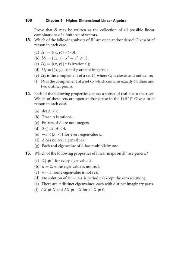
106 Chapter 5 Higher Dimensional Linear Algebra
Prove that S may be written as the collection of all possible linearcombinations of a finite set of vectors.
13. Which of the following subsets of Rn are open and/or dense? Give a briefreason in each case.
(a) U1 = {(x , y) | y > 0};(b) U2 = {(x , y) | x2 + y2 �= 1};(c) U3 = {(x , y) | x is irrational};(d) U4 = {(x , y) | x and y are not integers};(e) U5 is the complement of a set C1 where C1 is closed and not dense;
(f) U6 is the complement of a set C2 which contains exactly 6 billion andtwo distinct points.
14. Each of the following properties defines a subset of real n × n matrices.Which of these sets are open and/or dense in the L(Rn)? Give a briefreason in each case.
(a) det A �= 0.
(b) Trace A is rational.
(c) Entries of A are not integers.
(d) 3 ≤ det A < 4.
(e) −1 < |λ| < 1 for every eigenvalue λ.
(f) A has no real eigenvalues.
(g) Each real eigenvalue of A has multiplicity one.
15. Which of the following properties of linear maps on Rn are generic?
(a) |λ| �= 1 for every eigenvalue λ.
(b) n = 2; some eigenvalue is not real.
(c) n = 3; some eigenvalue is not real.
(d) No solution of X ′ = AX is periodic (except the zero solution).
(e) There are n distinct eigenvalues, each with distinct imaginary parts.
(f) AX �= X and AX �= −X for all X �= 0.

6Higher Dimensional
Linear Systems
After our little sojourn into the world of linear algebra, it’s time to return to dif-ferential equations and, in particular, to the task of solving higher dimensionallinear systems with constant coefficients. As in the linear algebra chapter, wehave to deal with a number of different cases.
6.1 Distinct Eigenvalues
Consider first a linear system X ′ = AX where the n × n matrix A has ndistinct, real eigenvalues λ1, . . . , λn . By the results in Chapter 5, there is achange of coordinates T so that the new system Y ′ = (T−1AT )Y assumes theparticularly simple form
y ′1 = λ1y1
...
y ′n = λnyn .
The linear map T is the map that takes the standard basis vector Ej to theeigenvector Vj associated to λj . Clearly, a function of the form
Y (t ) =⎛⎜⎝c1eλ1t
...cneλnt
⎞⎟⎠
107

108 Chapter 6 Higher Dimensional Linear Systems
is a solution of Y ′ = (T−1AT )Y that satisfies the initial condition Y (0) =(c1, . . . , cn). As in Chapter 3, this is the only such solution, because if
W (t ) =⎛⎜⎝w1(t )
...wn(t )
⎞⎟⎠
is another solution, then differentiating each expression wj(t ) exp(−λj t ), wefind
d
dtwj(t )e
−λj t = (w ′j − λjwj)e
−λj t = 0.
Hence wj(t ) = cj exp(λj t ) for each j . Therefore the collection of solutionsY (t ) yields the general solution of Y ′ = (T−1AT )Y .
It then follows that X(t ) = TY (t ) is the general solution of X ′ = AX , sothis general solution may be written in the form
X(t ) =n∑
j=1
cj eλj t Vj .
Now suppose that the eigenvalues λ1, . . . , λk of A are negative, while theeigenvalues λk+1, . . . , λn are positive. Since there are no zero eigenvalues, thesystem is hyperbolic. Then any solution that starts in the subspace spannedby the vectors V1, . . . , Vk must first of all stay in that subspace for all timesince ck+1 = · · · = cn = 0. Secondly, each such solution tends to the originas t → ∞. In analogy with the terminology introduced for planar systems,we call this subspace the stable subspace. Similarly, the subspace spanned byVk+1, . . . , Vn contains solutions that move away from the origin. This subspaceis the unstable subspace. All other solutions tend toward the stable subspaceas time goes backward and toward the unstable subspace as time increases.Therefore this system is a higher dimensional analog of a saddle.
Example. Consider
X ′ =⎛⎝1 2 −1
0 3 −20 2 −2
⎞⎠X .
In Section 5.2 in Chapter 5, we showed that this matrix has eigenvalues2, 1, and −1 with associated eigenvectors (3, 2, 1), (1, 0, 0), and (0, 1, 2),respectively. Therefore the matrix
T =⎛⎝3 1 0
2 0 11 0 2
⎞⎠

6.1 Distinct Eigenvalues 109
z
x
y
T(0, 1, 2)
Figure 6.1 The stable and unstable subspaces of a saddle in dimension 3.On the left, the system is in canonical form.
converts X ′ = AX to
Y ′ = (T−1AT )Y =⎛⎝2 0 0
0 1 00 0 −1
⎞⎠Y ,
which we can solve immediately. Multiplying the solution by T then yields thegeneral solution
X(t ) = c1e2t
⎛⎝3
21
⎞⎠ + c2et
⎛⎝1
00
⎞⎠ + c3e−t
⎛⎝0
12
⎞⎠
of X ′ = AX . The straight line through the origin and (0, 1, 2) is the stableline, while the plane spanned by (3, 2, 1) and (1, 0, 0) is the unstable plane. Acollection of solutions of this system as well as the system Y ′ = (T−1AT )Y isdisplayed in Figure 6.1. �
Example. If the 3 × 3 matrix A has three real, distinct eigenvalues that arenegative, then we may find a change of coordinates so that the system assumesthe form
Y ′ = (T−1AT )Y =⎛⎝λ1 0 0
0 λ2 00 0 λ3
⎞⎠Y
where λ3 < λ2 < λ1 < 0. All solutions therefore tend to the origin and sowe have a higher dimensional sink. See Figure 6.2. For an initial condition(x0, y0, z0) with all three coordinates nonzero, the corresponding solutiontends to the origin tangentially to the x-axis (see Exercise 2 at the end ofthe chapter). �

110 Chapter 6 Higher Dimensional Linear Systems
z
x
y
Figure 6.2 A sink in three dimensions.
Now suppose that the n × n matrix A has n distinct eigenvalues, of whichk1 are real and 2k2 are nonreal, so that n = k1 + 2k2. Then, as in Chapter 5,we may change coordinates so that the system assumes the form
x ′j = λj xj
u′� = α�u� + β�v�
v ′� = −β�u� + α�v�
for j = 1, . . . , k1 and � = 1, . . . , k2. As in Chapter 3, we therefore have solutionsof the form
xj(t ) = cj eλj t
u�(t ) = p�eα�t cos β�t + q�e
α�t sin β�t
v�(t ) = −p�eα�t sin β�t + q�e
α�t cos β�t .
As before, it is straightforward to check that this is the general solution. Wehave therefore shown:
Theorem. Consider the system X ′ = AX where A has distinct eigenvaluesλ1, . . . , λk1 ∈ R and α1 + iβ1, . . . , αk2 + iβk2 ∈ C. Let T be the matrix that putsA in the canonical form
T−1AT =
⎛⎜⎜⎜⎜⎜⎜⎜⎜⎝
λ1
. . .λk1
B1
. . .Bk2
⎞⎟⎟⎟⎟⎟⎟⎟⎟⎠

6.1 Distinct Eigenvalues 111
where
Bj =(
αj βj
−βj αj
).
Then the general solution of X ′ = AX is TY (t ) where
Y (t ) =
⎛⎜⎜⎜⎜⎜⎜⎜⎜⎜⎜⎜⎜⎝
c1eλ1t
...ckeλk1 t
a1eα1t cos β1t + b1eα1t sin β1t−a1eα1t sin β1t + b1eα1t cos β1t
...ak2e
αk2 t cos βk2 t + bk2eαk2 t sin βk2 t−ak2e
αk2 t sin βk2 t + bk2eαk2 t cos βk2 t
⎞⎟⎟⎟⎟⎟⎟⎟⎟⎟⎟⎟⎟⎠
�
As usual, the columns of the matrix T in this theorem are the eigenvectors(or the real and imaginary parts of the eigenvectors) corresponding to eacheigenvalue. Also, as before, the subspace spanned by the eigenvectors corre-sponding to eigenvalues with negative (resp., positive) real parts is the stable(resp., unstable) subspace.
Example. Consider the system
X ′ =⎛⎝ 0 1 0
−1 0 00 0 −1
⎞⎠X
whose matrix is already in canonical form. The eigenvalues are ±i, −1. Thesolution satisfying the initial condition (x0, y0, z0) is given by
Y (t ) = x0
⎛⎝ cos t
− sin t0
⎞⎠ + y0
⎛⎝sin t
cos t0
⎞⎠ + z0e−t
⎛⎝0
01
⎞⎠
so this is the general solution. The phase portrait for this system is displayedin Figure 6.3. The stable line lies along the z-axis, whereas all solutions in thexy–plane travel around circles centered at the origin. In fact, each solutionthat does not lie on the stable line actually lies on a cylinder in R3 given byx2 + y2 = constant. These solutions spiral toward the circular solution ofradius
√x2
0 + y20 in the xy–plane if z0 �= 0. �

112 Chapter 6 Higher Dimensional Linear Systems
x2�y2�a2
Figure 6.3 The phase portrait for a spiralcenter.
Example. Now consider X ′ = AX where
A =⎛⎝−0. 1 0 1
−1 1 −1. 1−1 0 −0. 1
⎞⎠ .
The characteristic equation is
−λ3 + 0. 8λ2 − 0. 81λ + 1. 01 = 0,
which we have kindly factored for you into
(1 − λ)(λ2 + 0. 2λ + 1. 01) = 0.
Therefore the eigenvalues are the roots of this equation, which are 1 and−0. 1±i. Solving (A − (−0. 1 + i)I )X = 0 yields the eigenvector (−i, 1, 1) associatedto −0. 1 + i. Let V1 = Re (−i, 1, 1) = (0, 1, 1) and V2 = Im (−i, 1, 1) =(−1, 0, 0). Solving (A − I )X = 0 yields V3 = (0, 1, 0) as an eigenvectorcorresponding to λ = 1. Then the matrix whose columns are the Vi ,
T =⎛⎝0 −1 0
1 0 11 0 0
⎞⎠ ,
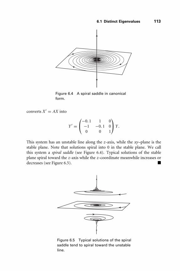
6.1 Distinct Eigenvalues 113
Figure 6.4 A spiral saddle in canonicalform.
converts X ′ = AX into
Y ′ =⎛⎝−0. 1 1 0
−1 −0. 1 00 0 1
⎞⎠Y .
This system has an unstable line along the z-axis, while the xy–plane is thestable plane. Note that solutions spiral into 0 in the stable plane. We callthis system a spiral saddle (see Figure 6.4). Typical solutions of the stableplane spiral toward the z-axis while the z-coordinate meanwhile increases ordecreases (see Figure 6.5). �
Figure 6.5 Typical solutions of the spiralsaddle tend to spiral toward the unstableline.

114 Chapter 6 Higher Dimensional Linear Systems
6.2 Harmonic Oscillators
Consider a pair of undamped harmonic oscillators whose equations are
x ′′1 = −ω2
1x1
x ′′2 = −ω2
2x2.
We can almost solve these equations by inspection as visions of sin ωt andcos ωt pass through our minds. But let’s push on a bit, first to illustrate thetheorem in the previous section in the case of nonreal eigenvalues, but moreimportantly to introduce some interesting geometry.
We first introduce the new variables yj = x ′j for j = 1, 2 so that the equations
can be written as a system
x ′j = yj
y ′j = −ω2
j xj .
In matrix form, this system is X ′ = AX where X = (x1, y1, x2, y2) and
A =
⎛⎜⎜⎝
0 1−ω2
1 00 1
−ω22 0
⎞⎟⎟⎠ .
This system has eigenvalues ±iω1 and ±iω2. An eigenvector corresponding toiω1 is V1 = (1, iω1, 0, 0) while V2 = (0, 0, 1, iω2) is associated to iω2. Let W1
and W2 be the real and imaginary parts of V1, and let W3 and W4 be the samefor V2. Then, as usual, we let TEj = Wj and the linear map T puts this systeminto canonical form with the matrix
T−1AT =
⎛⎜⎜⎝
0 ω1
−ω1 00 ω2
−ω2 0
⎞⎟⎟⎠ .
We then derive the general solution
Y (t ) =
⎛⎜⎜⎝
x1(t )y1(t )x2(t )y2(t )
⎞⎟⎟⎠ =
⎛⎜⎜⎝
a1 cos ω1t + b1 sin ω1t−a1 sin ω1t + b1 cos ω1ta2 cos ω2t + b2 sin ω2t
−a2 sin ω2t + b2 cos ω2t
⎞⎟⎟⎠
just as we originally expected.
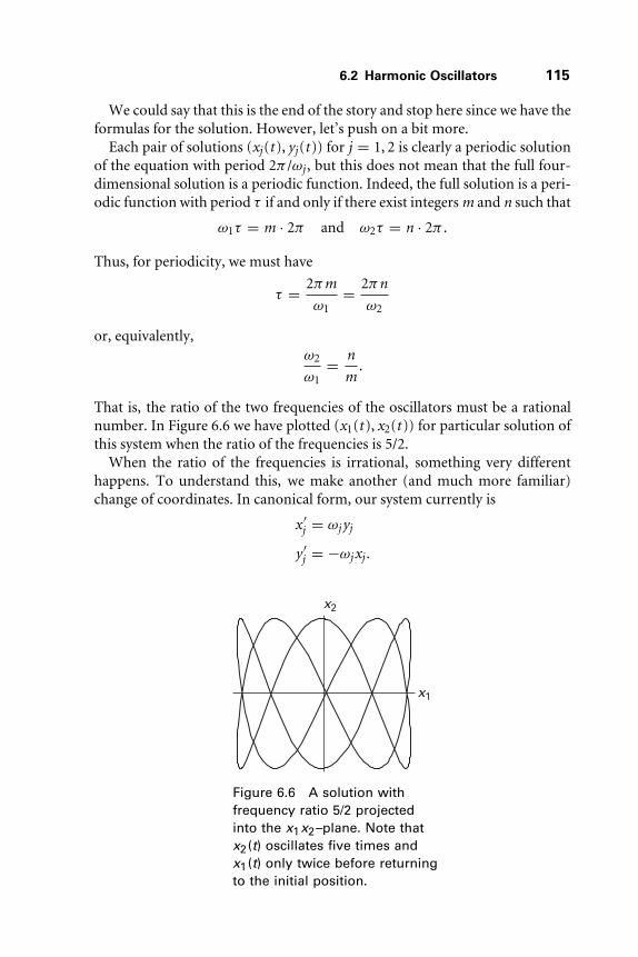
6.2 Harmonic Oscillators 115
We could say that this is the end of the story and stop here since we have theformulas for the solution. However, let’s push on a bit more.
Each pair of solutions (xj(t ), yj(t )) for j = 1, 2 is clearly a periodic solutionof the equation with period 2π /ωj , but this does not mean that the full four-dimensional solution is a periodic function. Indeed, the full solution is a peri-odic function with period τ if and only if there exist integers m and n such that
ω1τ = m · 2π and ω2τ = n · 2π .
Thus, for periodicity, we must have
τ = 2πm
ω1= 2πn
ω2
or, equivalently,ω2
ω1= n
m.
That is, the ratio of the two frequencies of the oscillators must be a rationalnumber. In Figure 6.6 we have plotted (x1(t ), x2(t )) for particular solution ofthis system when the ratio of the frequencies is 5/2.
When the ratio of the frequencies is irrational, something very differenthappens. To understand this, we make another (and much more familiar)change of coordinates. In canonical form, our system currently is
x ′j = ωj yj
y ′j = −ωj xj .
x2
x1
Figure 6.6 A solution withfrequency ratio 5/2 projectedinto the x1x2–plane. Note thatx2(t) oscillates five times andx1(t) only twice before returningto the initial position.
116 Chapter 6 Higher Dimensional Linear Systems
Let’s now introduce polar coordinates (rj , θj) in place of the xj and yj variables.Differentiating
r2j = x2
j + y2j ,
we find
2rj r′j = 2xjx
′j + 2yjy
′j
= 2xjyjωj − 2xjyjωj
= 0.
Therefore r ′j = 0 for each j . Also, differentiating the equation
tan θj = yj
xj
yields
(sec2θj)θ′j =
y ′j xj − yjx ′
j
x2j
=−ωj r2
j
r2j cos2 θj
from which we find
θ ′j = −ωj .
So, in polar coordinates, these equations really are quite simple:
r ′j = 0
θ ′j = −ωj .
The first equation tells us that both r1 and r2 remain constant along anysolution. Then, no matter what we pick for our initial r1 and r2 values, theθj equations remain the same. Hence we may as well restrict our attention tor1 = r2 = 1. The resulting set of points in R4 is a torus—the surface of adoughnut—although this is a little difficult to visualize in four-dimensionalspace. However, we know that we have two independent variables on this set,namely, θ1 and θ2, and both are periodic with period 2π . So this is akin tothe two independent circular directions that parameterize the familiar torusin R3.

6.2 Harmonic Oscillators 117
Restricted to this torus, the equations now read
θ ′1 = −ω1
θ ′2 = −ω2.
It is convenient to think of θ1 and θ2 as variables in a square of sidelength 2πwhere we glue together the opposite sides θj = 0 and θj = 2π to make thetorus. In this square our vector field now has constant slope
θ ′2
θ ′1
= ω2
ω1.
Therefore solutions lie along straight lines with slope ω2/ω1 in this square.When a solution reaches the edge θ1 = 2π (say, at θ2 = c), it instantlyreappears on the edge θ1 = 0 with the θ2 coordinate given by c , and thencontinues onward with slope ω2/ω1. A similar identification occurs when thesolution meets θ2 = 2π .
So now we have a simplified geometric vision of what happens to thesesolutions on these tori. But what really happens? The answer depends on theratio ω2/ω1. If this ratio is a rational number, say, n/m, then the solutionstarting at (θ1(0), θ2(0)) will pass horizontally through the torus exactly mtimes and vertically n times before returning to its starting point. This is theperiodic solution we observed above. Incidentally, the picture of the straightline solutions in the θ1θ2–plane is not at all the same as our depiction ofsolutions in the x1x2–plane as shown in Figure 6.6.
In the irrational case, something quite different occurs. See Figure 6.7. Tounderstand what is happening here, we return to the notion of a Poincaré mapdiscussed in Chapter 1. Consider the circle θ1 = 0, the left-hand edge of oursquare representation of the torus. Given an initial point on this circle, say,θ2 = x0, we follow the solution starting at this point until it next hits θ1 = 2π .
Figure 6.7 A solution with frequency ratio√
2projected into the x1x2–plane, the left curvecomputed up to time 50π , the right to time 100π .

118 Chapter 6 Higher Dimensional Linear Systems
x1�f (x0)
h1�0 h1�2π
x0x2
Figure 6.8 The Poincaré map on thecircle θ1 = 0 in the θ1θ2 torus.
By our identification, this solution has now returned to the circle θ1 = 0. Thesolution may cross the boundary θ2 = 2π several times in making this transit,but it does eventually return to θ1 = 0. So we may define the Poincaré mapon θ1 = 0 by assigning to x0 on this circle the corresponding coordinate of thepoint of first return. Suppose that this first return occurs at the point θ2(τ )where τ is the time for which θ1(τ ) = 2π . Since θ1(t ) = θ1(0) + ω1t , we haveτ = 2π /ω1. Hence θ2(τ ) = x0 + ω2(2π /ω1). Therefore the Poincaré map onthe circle may be written as
f (x0) = x0 + 2π(ω2/ω1) mod 2π
where x0 = θ2(0) is our initial θ2 coordinate on the circle. See Figure 6.8. Thusthe Poincaré map on the circle is just the function that rotates points on thecircle by angle 2π(ω2/ω1). Since ω2/ω1 is irrational, this function is called anirrational rotation of the circle.
Definition
The set of points x0, x1 = f (x0), x2 = f (f (x0)), . . . , xn = f (xn−1) iscalled the orbit of x0 under iteration of f .
The orbit of x0 tracks how our solution successively crosses θ1 = 2π as timeincreases.
Proposition. Suppose ω2/ω1 is irrational. Then the orbit of any initial pointx0 on the circle θ1 = 0 is dense in the circle.
Proof: Recall from Section 5.6 that a subset of the circle is dense if thereare points in this subset that are arbitrarily close to any point whatsoever

6.3 Repeated Eigenvalues 119
in the circle. Therefore we must show that, given any point z on the circle andany ε > 0, there is a point xn on the orbit of x0 such that |z − xn| < ε wherez and xn are measured mod 2π . To see this, observe first that there must ben, m for which m > n and |xn − xm| < ε. Indeed, we know that the orbitof x0 is not a finite set of points since ω2/ω1 is irrational. Hence there mustbe at least two of these points whose distance apart is less than ε since thecircle has finite circumference. These are the points xn and xm (actually, theremust be infinitely many such points). Now rotate these points in the reversedirection exactly n times. The points xn and xm are rotated to x0 and xm−n ,respectively. We find, after this rotation, that |x0 − xm−n| < ε. Now xm−n isgiven by rotating the circle through angle (m −n)2π(ω2/ω1), which, mod 2π ,is therefore a rotation of angle less than ε. Hence, performing this rotationagain, we find
|x2(m−n) − xm−n| < ε
as well, and, inductively,
|xk(m−n) − x(k−1)(m−n)| < ε
for each k. Thus we have found a sequence of points obtained by repeatedrotation through angle (m − n)2π(ω2/ω1), and each of these points iswithin ε of its predecessor. Hence there must be a point of this form withinε of z . �
Since the orbit of x0 is dense in the circle θ1 = 0, it follows that the straight-line solutions connecting these points in the square are also dense, and so theoriginal solutions are dense in the torus on which they reside. This accounts forthe densely packed solution shown projected into the x1x2–plane in Figure 6.7when ω2/ω1 = √
2.Returning to the actual motion of the oscillators, we see that when ω2/ω1
is irrational, the masses do not move in periodic fashion. However, they docome back very close to their initial positions over and over again as time goeson due to the density of these solutions on the torus. These types of motionsare called quasi-periodic motions. In Exercise 7 we investigate a related set ofequations, namely, a pair of coupled oscillators.
6.3 Repeated Eigenvalues
As we saw in the previous chapter, the solution of systems with repeatedreal eigenvalues reduces to solving systems whose matrices contain blocks

120 Chapter 6 Higher Dimensional Linear Systems
of the form ⎛⎜⎜⎜⎜⎜⎜⎝
λ 1λ 1
. . .. . .. . . 1
λ
⎞⎟⎟⎟⎟⎟⎟⎠ .
Example. Let
X ′ =⎛⎝λ 1 0
0 λ 10 0 λ
⎞⎠X .
The only eigenvalue for this system is λ, and its only eigenvector is (1, 0, 0).We may solve this system as we did in Chapter 3, by first noting that x ′
3 = λx3,so we must have
x3(t ) = c3eλt .
Now we must have
x ′2 = λx2 + c3eλt .
As in Chapter 3, we guess a solution of the form
x2(t ) = c2eλt + αteλt .
Substituting this guess into the differential equation for x ′2, we determine that
α = c3 and find
x2(t ) = c2eλt + c3teλt .
Finally, the equation
x ′1 = λx1 + c2eλt + c3teλt
suggests the guess
x1(t ) = c1eλt + αteλt + βt 2eλt .
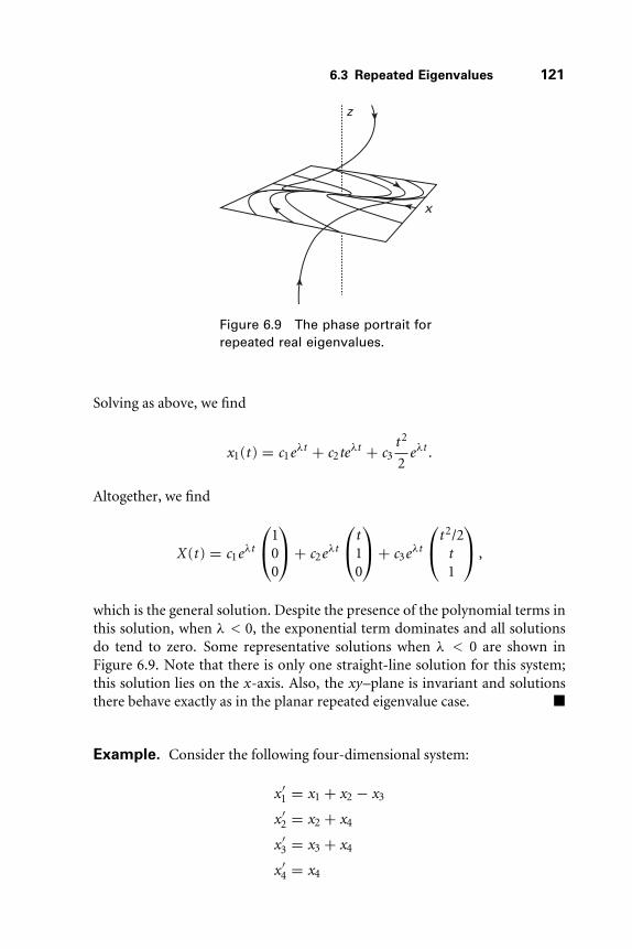
6.3 Repeated Eigenvalues 121
x
z
Figure 6.9 The phase portrait forrepeated real eigenvalues.
Solving as above, we find
x1(t ) = c1eλt + c2teλt + c3t 2
2eλt .
Altogether, we find
X(t ) = c1eλt
⎛⎝1
00
⎞⎠ + c2eλt
⎛⎝t
10
⎞⎠ + c3eλt
⎛⎝t 2/2
t1
⎞⎠ ,
which is the general solution. Despite the presence of the polynomial terms inthis solution, when λ < 0, the exponential term dominates and all solutionsdo tend to zero. Some representative solutions when λ < 0 are shown inFigure 6.9. Note that there is only one straight-line solution for this system;this solution lies on the x-axis. Also, the xy–plane is invariant and solutionsthere behave exactly as in the planar repeated eigenvalue case. �
Example. Consider the following four-dimensional system:
x ′1 = x1 + x2 − x3
x ′2 = x2 + x4
x ′3 = x3 + x4
x ′4 = x4

122 Chapter 6 Higher Dimensional Linear Systems
We may write this system in matrix form as
X ′ = AX =
⎛⎜⎜⎝
1 1 −1 00 1 0 10 0 1 10 0 0 1
⎞⎟⎟⎠X .
Because A is upper triangular, all of the eigenvalues are equal to 1. Solving(A − I )X = 0, we find two independent eigenvectors V1 = (1, 0, 0, 0) andW1 = (0, 1, 1, 0). This reduces the possible canonical forms for A to twopossibilities. Solving (A − I )X = V1 yields one solution V2 = (0, 1, 0, 0), andsolving (A − I )X = W1 yields another solution W2 = (0, 0, 0, 1). Thus weknow that the system X ′ = AX may be tranformed into
Y ′ = (T−1AT )Y =
⎛⎜⎜⎝
1 1 0 00 1 0 00 0 1 10 0 0 1
⎞⎟⎟⎠Y
where the matrix T is given by
T =
⎛⎜⎜⎝
1 0 0 00 1 1 00 0 1 00 0 0 1
⎞⎟⎟⎠ .
Solutions of Y ′ = (T−1AT )Y therefore are given by
y1(t ) = c1et + c2tet
y2(t ) = c2et
y3(t ) = c3et + c4tet
y4(t ) = c4et .
Applying the change of coordinates T , we find the general solution of theoriginal system
x1(t ) = c1et + c2tet
x2(t ) = c2et + c3et + c4tet
x3(t ) = c3et + c4tet
x4(t ) = c4et . �

6.4 The Exponential of a Matrix 123
6.4 The Exponential of a Matrix
We turn now to an alternative and elegant approach to solving linear systemsusing the exponential of a matrix. In a certain sense, this is the more naturalway to attack these systems.
Recall from Section 1.1 in Chapter 1 how we solved the 1 × 1 “system” oflinear equations x ′ = ax where our matrix was now simply (a). We did notgo through the process of finding eigenvalues and eigenvectors here. (Well,actually, we did, but the process was pretty simple.) Rather, we just exponen-tiated the matrix (a) to find the general solution x(t ) = c exp(at ). In fact, thisprocess works in the general case where A is n ×n. All we need to know is howto exponentiate a matrix.
Here’s how: Recall from calculus that the exponential function can beexpressed as the infinite series
ex =∞∑
k=0
xk
k! .
We know that this series converges for every x ∈ R. Now we can add matrices,we can raise them to the power k, and we can multiply each entry by 1/k!. Sothis suggests that we can use this series to exponentiate them as well.
Definition
Let A be an n ×n matrix. We define the exponential of A to be thematrix given by
exp(A) =∞∑
k=0
Ak
k! .
Of course we have to worry about what it means for this sum of matrices toconverge, but let’s put that off and try to compute a few examples first.
Example. Let
A =(
λ 00 μ
).
Then we have
Ak =(
λk 00 μk
)

124 Chapter 6 Higher Dimensional Linear Systems
so that
exp(A) =
⎛⎜⎜⎜⎜⎝
∞∑k=0
λk /k! 0
0∞∑
k=0
μk /k!
⎞⎟⎟⎟⎟⎠ =
(eλ 00 eμ
)
as you may have guessed. �
Example. For a slightly more complicated example, let
A =(
0 β
−β 0
).
We compute
A0 = I , A2 = −β2I , A3 = −β3(
0 1−1 0
),
A4 = β4I , A5 = β5(
0 1−1 0
), . . .
so we find
exp(A) =
⎛⎜⎜⎜⎜⎜⎜⎜⎜⎝
∞∑k=0
(−1)k β2k
(2k)!∞∑
k=0
(−1)k β2k+1
(2k + 1)!
−∞∑
k=0
(−1)k β2k+1
(2k + 1)!∞∑
k=0
(−1)k β2k
(2k)!
⎞⎟⎟⎟⎟⎟⎟⎟⎟⎠
=(
cos β sin β
− sin β cos β
). �
Example. Now let
A =(
λ 10 λ
)

6.4 The Exponential of a Matrix 125
with λ �= 0. With an eye toward what comes later, we compute, not exp A, butrather exp(tA). We have
(tA)k =(
(tλ)k kt kλk−1
0 (tλ)k
).
Hence we find
exp(tA) =
⎛⎜⎜⎜⎜⎜⎜⎝
∞∑k=0
(tλ)k
k! t∞∑
k=0
(tλ)k
k!
0∞∑
k=0
(tλ)k
k!
⎞⎟⎟⎟⎟⎟⎟⎠ =
(etλ tetλ
0 etλ
).
�
Note that, in each of these three examples, the matrix exp(A) is a matrixwhose entries are infinite series. We therefore say that the infinite series ofmatrices exp(A) converges absolutely if each of its individual terms does so. Ineach of the previous cases, this convergence was clear. Unfortunately, in thecase of a general matrix A, this is not so clear. To prove convergence here, weneed to work a little harder.
Let aij(k) denote the ij entry of Ak . Let a = max |aij |. We have
|aij(2)| =∣∣∣∣ n∑
k=1
aikakj
∣∣∣∣ ≤ na2
|aij(3)| =∣∣∣∣ n∑
k,�=1
aikak�a�j
∣∣∣∣ ≤ n2a3
...
|aij(k)| ≤ nk−1ak .
Hence we have a bound for the ij entry of the n × n matrix exp(A):
∣∣∣∣ ∞∑k=0
aij(k)
k!∣∣∣∣ ≤
∞∑k=0
|aij(k)|k! ≤
∞∑k=0
nk−1ak
k! ≤∞∑
k=0
(na)k
k! ≤ exp na
so that this series converges absolutely by the comparison test. Therefore thematrix exp A makes sense for any A ∈ L(Rn).
The following result shows that matrix exponentiation shares many of thefamiliar properties of the usual exponential function.
126 Chapter 6 Higher Dimensional Linear Systems
Proposition. Let A, B, and T be n × n matrices. Then:
1. If B = T−1AT, then exp(B) = T−1 exp(A)T.2. If AB = BA, then exp(A + B) = exp(A) exp(B).3. exp(−A) = (exp(A))−1.
Proof: The proof of (1) follows from the identities T−1(A+B)T = T−1AT +T−1BT and (T−1AT )k = T−1AkT . Therefore
T−1
(n∑
k=0
Ak
k!
)T =
n∑k=0
(T−1AT
)k
k!
and (1) follows by taking limits.To prove (2), observe that because AB = BA we have, by the binomial
theorem,
(A + B)n = n!∑
j+k=n
Aj
j!Bk
k! .
Therefore we must show that
∞∑n=0
⎛⎝ ∑
j+k=n
Aj
j!Bk
k!
⎞⎠ =
⎛⎝ ∞∑
j=0
Aj
j!
⎞⎠( ∞∑
k=0
Bk
k!
).
This is not as obvious as it may seem, since we are dealing here with seriesof matrices, not series of real numbers. So we will prove this in the followinglemma, which then proves (2). Putting B = −A in (2) gives (3). �
Lemma. For any n × n matrices A and B, we have:
∞∑n=0
⎛⎝ ∑
j+k=n
Aj
j!Bk
k!
⎞⎠ =
⎛⎝ ∞∑
j=0
Aj
j!
⎞⎠( ∞∑
k=0
Bk
k!
).
Proof: We know that each of these infinite series of matrices converges. Wejust have to check that they converge to each other. To do this, consider thepartial sums
γ2m =2m∑n=0
⎛⎝ ∑
j+k=n
Aj
j!Bk
k!
⎞⎠

6.4 The Exponential of a Matrix 127
and
αm =⎛⎝ m∑
j=0
Aj
j!
⎞⎠ and βm =
(m∑
k=0
Bk
k!
).
We need to show that the matrices γ2m − αmβm tend to the zero matrix asm → ∞. Toward that end, for a matrix M = [mij ], we let ||M || = max |mij |.We will show that ||γ2m − αmβm|| → 0 as m → ∞.
A computation shows that
γ2m − αmβm =∑′ Aj
j!Bk
k! +∑′′ Aj
j!Bk
k!where
∑′ denotes the sum over terms with indices satisfying
j + k ≤ 2m, 0 ≤ j ≤ m, m + 1 ≤ k ≤ 2m
while∑′′ is the sum corresponding to
j + k ≤ 2m, m + 1 ≤ j ≤ 2m, 0 ≤ k ≤ m.
Therefore
||γ2m − αmβm|| ≤∑′ ∣∣∣∣Aj
j!∣∣∣∣ · ∣∣∣∣Bk
k!∣∣∣∣ +
∑′′ ∣∣∣∣Aj
j!∣∣∣∣ · ∣∣∣∣Bk
k!∣∣∣∣.
Now
∑′ ∣∣∣∣Aj
j!∣∣∣∣ · ∣∣∣∣Bk
k!∣∣∣∣ ≤
( m∑j=0
∣∣∣∣Aj
j!∣∣∣∣)( 2m∑
k=m+1
∣∣∣∣Bk
k!∣∣∣∣).
This tends to 0 as m → ∞ since, as we saw above,
∞∑j=0
∣∣∣∣Aj
j!∣∣∣∣ ≤ exp(n||A||) < ∞.
Similarly,
∑′′ ∣∣∣∣Aj
j!∣∣∣∣ · ∣∣∣∣Bk
k!∣∣∣∣ → 0
as m → ∞. Therefore limm→∞(γ2m − αmβm) = 0, proving the lemma. �

128 Chapter 6 Higher Dimensional Linear Systems
Observe that statement (3) of the proposition implies that exp(A) isinvertible for every matrix A. This is analogous to the fact that ea �= 0 forevery real number a.
There is a very simple relationship between the eigenvectors of A and thoseof exp(A).
Proposition. If V ∈ Rn is an eigenvector of A associated to the eigenvalue λ,then V is also an eigenvector of exp(A) associated to eλ.
Proof: From AV = λV , we obtain
exp(A)V = limn→∞
(n∑
k=0
AkV
k!
)
= limn→∞
(n∑
k=0
λk
k! V
)
=( ∞∑
k=0
λk
k!
)V
= eλV . �
Now let’s return to the setting of systems of differential equations. Let A bean n × n matrix and consider the system X ′ = AX . Recall that L(Rn) denotesthe set of all n × n matrices. We have a function R → L(Rn), which assigns
the matrix exp(tA) to t ∈ R. Since L(Rn) is identified with Rn2, it makes sense
to speak of the derivative of this function.
Proposition.
d
dtexp(tA) = A exp(tA) = exp(tA)A.
In other words, the derivative of the matrix-valued function t → exp(tA)is another matrix-valued function A exp(tA).
Proof: We have
d
dtexp(tA) = lim
h→0
exp((t + h)A) − exp(tA)
h
= limh→0
exp(tA) exp(hA) − exp(tA)
h

6.4 The Exponential of a Matrix 129
= exp(tA) limh→0
(exp(hA) − I
h
)= exp(tA)A;
that the last limit equals A follows from the series definition of exp(hA). Notethat A commutes with each term of the series for exp(tA), hence with exp(tA).This proves the proposition. �
Now we return to solving systems of differential equations. The followingmay be considered as the fundamental theorem of linear differential equationswith constant coefficients.
Theorem. Let A be an n × n matrix. Then the solution of the initial valueproblem X ′ = AX with X(0) = X0 is X(t ) = exp(tA)X0. Moreover, this is theonly such solution.
Proof: The preceding proposition shows that
d
dt(exp(tA)X0) =
(d
dtexp(tA)
)X0 = A exp(tA)X0.
Moreover, since exp(0A)X0 = X0, it follows that this is a solution of the initialvalue problem. To see that there are no other solutions, let Y (t ) be anothersolution satisfying Y (0) = X0 and set
Z (t ) = exp(−tA)Y (t ).
Then
Z ′(t ) =(
d
dtexp(−tA)
)Y (t ) + exp(−tA)Y ′(t )
= −A exp(−tA)Y (t ) + exp(−tA)AY (t )
= exp(−tA)(−A + A)Y (t )
≡ 0.
Therefore Z (t ) is a constant. Setting t = 0 shows Z (t ) = X0, so that Y (t ) =exp(tA)X0. This completes the proof of the theorem. �
Note that this proof is identical to that given way back in Section 1.1. Only themeaning of the letter A has changed.

130 Chapter 6 Higher Dimensional Linear Systems
Example. Consider the system
X ′ =(
λ 10 λ
)X .
By the theorem, the general solution is
X(t ) = exp(tA)X0 = exp
(tλ t0 tλ
)X0.
But this is precisely the matrix whose exponential we computed earlier. Wefind
X(t ) =(
etλ tetλ
0 etλ
)X0.
Note that this agrees with our computations in Chapter 3. �
6.5 Nonautonomous Linear Systems
Up to this point, virtually all of the linear systems of differential equationsthat we have encountered have been autonomous. There are, however, certaintypes of nonautonomous systems that often arise in applications. One suchsystem is of the form
X ′ = A(t )X
where A(t ) = [aij(t )] is an n × n matrix that depends continuously on time.We will investigate these types of systems further when we encounter thevariational equation in subsequent chapters.
Here we restrict our attention to a different type of nonautonomous linearsystem given by
X ′ = AX + G(t )
where A is a constant n × n matrix and G : R → Rn is a forcing termthat depends explicitly on t . This is an example of a first-order, linear,nonhomogeneous system of equations.

6.5 Nonautonomous Linear Systems 131
Example. (Forced Harmonic Oscillator) If we apply an external forceto the harmonic oscillator system, the differential equation governing themotion becomes
x ′′ + bx ′ + kx = f (t )
where f (t ) measures the external force. An important special case occurs whenthis force is a periodic function of time, which corresponds, for example, tomoving the table on which the mass-spring apparatus resides back and forthperiodically. As a system, the forced harmonic oscillator equation becomes
X ′ =(
0 1−k −b
)X + G(t ) where G(t ) =
(0
f (t )
). �
For a nonhomogeneous system, the equation that results from dropping thetime-dependent term, namely, X ′ = AX , is called the homogeneous equation.We know how to find the general solution of this system. Borrowing thenotation from the previous section, the solution satisfying the initial conditionX(0) = X0 is
X(t ) = exp(tA)X0,
so this is the general solution of the homogeneous equation.To find the general solution of the nonhomogeneous equation, suppose
that we have one particular solution Z (t ) of this equation. So Z ′(t ) =AZ (t ) + G(t ). If X(t ) is any solution of the homogeneous equation, thenthe function Y (t ) = X(t ) + Z (t ) is another solution of the nonhomogeneousequation. This follows since we have
Y ′ = X ′ + Z ′ = AX + AZ + G(t )
= A(X + Z ) + G(t )
= AY + G(t ).
Therefore, since we know all solutions of the homogeneous equation, we cannow find the general solution to the nonhomogeneous equation, providedthat we can find just one particular solution of this equation. Often one getssuch a solution by simply guessing that solution (in calculus, this method isusually called the method of undetermined coefficients). Unfortunately, guessinga solution does not always work. The following method, called variation ofparameters, does work in all cases. However, there is no guarantee that we canactually evaluate the required integrals.

132 Chapter 6 Higher Dimensional Linear Systems
Theorem. (Variation of Parameters) Consider the nonhomogeneousequation
X ′ = AX + G(t )
where A is an n × n matrix and G(t ) is a continuous function of t . Then
X(t ) = exp(tA)
(X0 +
∫ t
0exp(−sA) G(s) ds
)
is a solution of this equation satisfying X(0) = X0.
Proof: Differentiating X(t ), we obtain
X ′(t ) = A exp(tA)
(X0 +
∫ t
0exp(−sA) G(s) ds
)
+ exp(tA)d
dt
∫ t
0exp(−sA) G(s) ds
= A exp(tA)
(X0 +
∫ t
0exp(−sA) G(s) ds
)+ G(t )
= AX(t ) + G(t ). �
We now give several applications of this result in the case of the periodicallyforced harmonic oscillator. Assume first that we have a damped oscillator thatis forced by cos t , so the period of the forcing term is 2π . The system is
X ′ = AX + G(t )
where G(t ) = (0, cos t ) and A is the matrix
A =(
0 1−k −b
)
with b, k > 0. We claim that there is a unique periodic solution of this systemthat has period 2π . To prove this, we must first find a solution X(t ) satisfyingX(0) = X0 = X(2π). By variation of parameters, we need to find X0 such that
X0 = exp(2πA)X0 + exp(2πA)
∫ 2π
0exp(−sA) G(s) ds.
Now the term
exp(2πA)
∫ 2π
0exp(−sA) G(s) ds

6.5 Nonautonomous Linear Systems 133
is a constant vector, which we denote by W . Therefore we must solve theequation
(exp(2πA) − I
)X0 = −W .
There is a unique solution to this equation, since the matrix exp(2πA) − Iis invertible. For if this matrix were not invertible, we would have a nonzerovector V with
(exp(2πA) − I
)V = 0,
or, in other words, the matrix exp(2πA) would have an eigenvalue of 1. But,from the previous section, the eigenvalues of exp(2πA) are given by exp(2πλj)where the λj are the eigenvalues of A. But each λj has real part less than 0, sothe magnitude of exp(2πλj) is smaller than 1. Thus the matrix exp(2πA) − Iis indeed invertible, and the unique initial value leading to a 2π-periodicsolution is
X0 = (exp(2πA) − I
)−1(−W ).
So let X(t ) be this periodic solution with X(0) = X0. This solution is calledthe steady-state solution. If Y0 is any other initial condition, then we may writeY0 = (Y0 − X0) + X0, so the solution through Y0 is given by
Y (t ) = exp(tA)(Y0 − X0) + exp(tA)X0 + exp(tA)
∫ t
0exp(−sA) G(s) ds
= exp(tA)(Y0 − X0) + X(t ).
The first term in this expression tends to 0 as t → ∞, since it is a solutionof the homogeneous equation. Hence every solution of this system tends tothe steady-state solution as t → ∞. Physically, this is clear: The motion ofthe damped (and unforced) oscillator tends to equilibrium, leaving only themotion due to the periodic forcing. We have proved:
Theorem. Consider the forced, damped harmonic oscillator equation
x ′′ + bx ′ + kx = cos t
with k, b > 0. Then all solutions of this equation tend to the steady-state solution,which is periodic with period 2π . �

134 Chapter 6 Higher Dimensional Linear Systems
Now consider a particular example of a forced, undamped harmonicoscillator
X ′ =(
0 1−1 0
)X +
(0
cos ωt
)
where the period of the forcing is now 2π /ω with ω �= ±1. Let
A =(
0 1−1 0
).
The solution of the homogeneous equation is
X(t ) = exp(tA)X0 =(
cos t sin t− sin t cos t
)X0.
Variation of parameters provides a solution of the nonhomogeneous equationstarting at the origin:
Y (t ) = exp(tA)
∫ t
0exp(−sA)
(0
cos ωs
)ds
= exp(tA)
∫ t
0
(cos s − sin ssin s cos s
)(0
cos ωs
)ds
= exp(tA)
∫ t
0
(− sin s cos ωscos s cos ωs
)ds
= 1
2exp(tA)
∫ t
0
(sin(ω − 1)s − sin(ω + 1)scos(ω − 1)s + cos(ω + 1)s
)ds.
Recalling that
exp(tA) =(
cos t sin t− sin t cos t
)

Exercises 135
and using the fact that ω �= ±1, evaluation of this integral plus a longcomputation yields
Y (t ) = 1
2exp(tA)
⎛⎜⎜⎝
− cos(ω − 1)t
ω − 1+ cos(ω + 1)t
ω + 1sin(ω − 1)t
ω − 1+ sin(ω + 1)t
ω + 1
⎞⎟⎟⎠
+ exp(tA)
((ω2 − 1)−1
0
)
= 1
ω2 − 1
(− cos ωtω sin ωt
)+ exp(tA)
((ω2 − 1)−1
0
).
Thus the general solution of this equation is
Y (t ) = exp(tA)
(X0 +
((ω2 − 1)−1
0
))+ 1
ω2 − 1
(− cos ωtω sin ωt
).
The first term in this expression is periodic with period 2π while the secondhas period 2π /ω. Unlike the damped case, this solution does not necessarilyyield a periodic motion. Indeed, this solution is periodic if and only if ω is arational number. If ω is irrational, the motion is quasiperiodic, just as we sawin Section 6.2.
E X E R C I S E S
1. Find the general solution for X ′ = AX where A is given by:
(a)
⎛⎝0 0 1
0 1 01 0 0
⎞⎠ (b)
⎛⎝1 0 1
0 1 01 0 1
⎞⎠ (c)
⎛⎝ 0 1 0
−1 0 01 1 1
⎞⎠
(d)
⎛⎝0 1 0
1 0 01 1 1
⎞⎠ (e)
⎛⎝1 0 1
0 1 00 0 1
⎞⎠ (f )
⎛⎝1 1 0
1 1 10 1 1
⎞⎠
(g)
⎛⎝ 1 0 −1
−1 1 −10 0 1
⎞⎠ (h)
⎛⎜⎜⎝
1 0 0 10 1 1 00 0 1 01 0 0 0
⎞⎟⎟⎠

136 Chapter 6 Higher Dimensional Linear Systems
2. Consider the linear system
X ′ =⎛⎝λ1 0 0
0 λ2 00 0 λ3
⎞⎠X
where λ3 < λ2 < λ1 < 0. Describe how the solution through an arbitraryinitial value tends to the origin.
3. Give an example of a 3 × 3 matrix A for which all nonequilibriumsolutions of X ′ = AX are periodic with period 2π . Sketch the phaseportrait.
4. Find the general solution of
X ′ =
⎛⎜⎜⎝
0 1 1 0−1 0 0 10 0 0 10 0 −1 0
⎞⎟⎟⎠X .
5. Consider the system
X ′ =⎛⎝0 0 a
0 b 0a 0 0
⎞⎠X
depending on the two parameters a and b.
(a) Find the general solution of this system.
(b) Sketch the region in the ab–plane where this system has differenttypes of phase portraits.
6. Consider the system
X ′ =⎛⎝ a 0 b
0 b 0−b 0 a
⎞⎠X
depending on the two parameters a and b.
(a) Find the general solution of this system.
(b) Sketch the region in the ab–plane where this system has differenttypes of phase portraits.
7. Coupled Harmonic Oscillators. In this series of exercises you are askedto generalize the material on harmonic oscillators in Section 6.2 to thecase where the oscillators are coupled. Suppose there are two masses m1

Exercises 137
k1k2k1
m1 m2
Figure 6.10 A coupled oscillator.
and m2 attached to springs and walls as shown in Figure 6.10. The springsconnecting mj to the walls both have spring constants k1, while the springconnecting m1 and m2 has spring constant k2. This coupling means thatthe motion of either mass affects the behavior of the other.
Let xj denote the displacement of each mass from its rest position, andassume that both masses are equal to 1. The differential equations forthese coupled oscillators are then given by
x ′′1 = −(k1 + k2)x1 + k2x2
x ′′2 = k2x1 − (k1 + k2)x2.
These equations are derived as follows. If m1 is moved to the right(x1 > 0), the left spring is stretched and exerts a restorative force onm1 given by −k1x1. Meanwhile, the central spring is compressed, so itexerts a restorative force on m1 given by −k2x1. If the right spring isstretched, then the central spring is compressed and exerts a restorativeforce on m1 given by k2x2 (since x2 < 0). The forces on m2 are similar.
(a) Write these equations as a first-order linear system.
(b) Determine the eigenvalues and eigenvectors of the correspondingmatrix.
(c) Find the general solution.
(d) Let ω1 = √k1 and ω2 = √
k1 + 2k2. What can be said about theperiodicity of solutions relative to the ωj ? Prove this.
8. Suppose X ′ = AX where A is a 4×4 matrix whose eigenvalues are ±i√
2and ±i
√3. Describe this flow.
9. Suppose X ′ = AX where A is a 4 × 4 matrix whose eigenvalues are ±iand −1 ± i. Describe this flow.
10. Suppose X ′ = AX where A is a 4 × 4 matrix whose eigenvalues are ±iand ±1. Describe this flow.
11. Consider the system X ′ = AX where X = (x1, . . . , x6) and
A =
⎛⎜⎜⎜⎜⎜⎜⎝
0 ω1
−ω1 00 ω2
−ω2 0−1
1
⎞⎟⎟⎟⎟⎟⎟⎠

138 Chapter 6 Higher Dimensional Linear Systems
and ω1/ω2 is irrational. Describe qualitatively how a solution behaveswhen, at time 0, each xj is nonzero with the exception that
(a) x6 = 0;
(b) x5 = 0;
(c) x3 = x4 = x5 = 0;
(d) x3 = x4 = x5 = x6 = 0.
12. Compute the exponentials of the following matrices:
(a)
(5 −63 −4
)(b)
(2 −11 2
)(c)
(2 −10 2
)(d)
(0 11 0
)
(e)
⎛⎝0 1 2
0 0 30 0 0
⎞⎠ (f )
⎛⎝2 0 0
0 3 00 1 3
⎞⎠ (g)
⎛⎝λ 0 0
1 λ 00 1 λ
⎞⎠
(h)
(i 00 −i
)(i)
(1 + i 0
2 1 + i
)(j)
⎛⎜⎜⎝
1 0 0 01 0 0 01 0 0 01 0 0 0
⎞⎟⎟⎠
13. Find an example of two matrices A, B such that
exp(A + B) �= exp(A) exp(B).
14. Show that if AB = BA, then
(a) exp(A) exp(B) = exp(B) exp(A)
(b) exp(A)B = B exp(A).
15. Consider the triplet of harmonic oscillators
x ′′1 = −x1
x ′′2 = −2x2
x ′′3 = −ω2x3
where ω is irrational. What can you say about the qualitative behavior ofsolutions of this six-dimensional system?

7Nonlinear Systems
In this chapter we begin the study of nonlinear differential equations. Unlikelinear (constant coefficient) systems, where we can always find the explicitsolution of any initial value problem, this is rarely the case for nonlinear sys-tems. In fact, basic properties such as the existence and uniqueness of solutions,which was so obvious in the linear case, no longer hold for nonlinear systems.As we shall see, some nonlinear systems have no solutions whatsoever to agiven initial value problem. On the other hand, some systems have infinitelymany different such solutions. Even if we do find a solution of such a sys-tem, this solution need not be defined for all time; for example, the solutionmay tend to ∞ in finite time. And other questions arise: For example, whathappens if we vary the initial condition of a system ever so slightly? Does thecorresponding solution vary continuously? All of this is clear for linear sys-tems, but not at all clear in the nonlinear case. This means that the underlyingtheory behind nonlinear systems of differential equations is quite a bit morecomplicated than that for linear systems.
In practice, most nonlinear systems that arise are “nice” in the sense that wedo have existence and uniqueness of solutions as well as continuity of solutionswhen initial conditions are varied, and other “natural” properties. Thus wehave a choice: Given a nonlinear system, we could simply plunge ahead andeither hope that or, if possible, verify that, in each specific case, the system’ssolutions behave nicely. Alternatively, we could take a long pause at this stageto develop the necessary hypotheses that guarantee that solutions of a givennonlinear system behave nicely.
139

140 Chapter 7 Nonlinear Systems
In this book we pursue a compromise route. In this chapter, we will spellout in precise detail many of the theoretical results that govern the behaviorof solutions of differential equations. We will present examples of how andwhen these results fail, but we will not prove these theorems here. Rather,we will postpone all of the technicalities until Chapter 17, primarily becauseunderstanding this material demands a firm and extensive background in theprinciples of real analysis. In subsequent chapters, we will make use of theresults stated here, but readers who are primarily interested in applications ofdifferential equations or in understanding how specific nonlinear systems maybe analyzed need not get bogged down in these details here. Readers who wantthe technical details may take a detour to Chapter 17 now.
7.1 Dynamical Systems
As mentioned previously, most nonlinear systems of differential equations areimpossible to solve analytically. One reason for this is the unfortunate factthat we simply do not have enough functions with specific names that wecan use to write down explicit solutions of these systems. Equally problem-atic is the fact that, as we shall see, higher dimensional systems may exhibitchaotic behavior, a property that makes knowing a particular explicit solutionessentially worthless in the larger scheme of understanding the behavior of thesystem. Hence we are forced to resort to different means in order to understandthese systems. These are the techniques that arise in the field of dynamicalsystems. We will use a combination of analytic, geometric, and topologicaltechniques to derive rigorous results about the behavior of solutions of theseequations.
We begin by collecting some of the terminology regarding dynamical sys-tems that we have introduced at various points in the preceding chapters. Adynamical system is a way of describing the passage in time of all points of agiven space S . The space S could be thought of, for example, as the space ofstates of some physical system. Mathematically, S might be a Euclidean spaceor an open subset of Euclidean space or some other space such as a surface inR3. When we consider dynamical systems that arise in mechanics, the space Swill be the set of possible positions and velocities of the system. For the sake ofsimplicity, we will assume throughout that the space S is Euclidean space Rn ,although in certain cases the important dynamical behavior will be confinedto a particular subset of Rn .
Given an initial position X ∈ Rn , a dynamical system on Rn tells us whereX is located 1 unit of time later, 2 units of time later, and so on. We denotethese new positions of X by X1, X2, and so forth. At time zero, X is locatedat position X0. One unit before time zero, X was at X−1. In general, the

7.1 Dynamical Systems 141
“trajectory” of X is given by Xt . If we measure the positions Xt using onlyinteger time values, we have an example of a discrete dynamical system, whichwe shall study in Chapter 15. If time is measured continuously with t ∈ R,we have a continuous dynamical system. If the system depends on time ina continuously differentiable manner, we have a smooth dynamical system.These are the three principal types of dynamical systems that arise in thestudy of systems of differential equations, and they will form the backbone ofChapters 8 through 14.
The function that takes t to Xt yields either a sequence of points or a curvein Rn that represents the life history of X as time runs from −∞ to ∞.Different branches of dynamical systems make different assumptions abouthow the function Xt depends on t . For example, ergodic theory deals withsuch functions under the assumption that they preserve a measure on Rn .Topological dynamics deals with such functions under the assumption thatXt varies only continuously. In the case of differential equations, we willusually assume that the function Xt is continuously differentiable. The mapφt : Rn → Rn that takes X into Xt is defined for each t and, from ourinterpretation of Xt as a state moving in time, it is reasonable to expect φt tohave φ−t as its inverse. Also, φ0 should be the identity function φ0(X) = Xand φt (φs(X)) = φt+s(X) is also a natural condition. We formalize all of thisin the following definition:
Definition
A smooth dynamical system on Rn is a continuously differentiablefunction φ : R × Rn → Rn where φ(t , X) = φt (X) satisfies
1. φ0: Rn → Rn is the identity function: φ0(X0) = X0;2. The composition φt ◦ φs = φt+s for each t , s ∈ R.
Recall that a function is continuously differentiable if all of its partial deriva-tives exist and are continuous throughout its domain. It is traditional to call acontinuously differentiable function a C1 function. If the function is k timescontinuously differentiable, it is called a Ck function. Note that the definitionabove implies that the map φt : Rn → Rn is C1 for each t and has a C1 inverseφ−t (take s = −t in part 2).
Example. For the first-order differential equation x ′ = ax , the functionφt (x0) = x0 exp(at ) gives the solutions of this equation and also defines asmooth dynamical system on R. �
Example. Let A be an n × n matrix. Then the function φt (X0) = exp(tA)X0
defines a smooth dynamical system on Rn . Clearly, φ0 = exp(0) = I and, as

142 Chapter 7 Nonlinear Systems
we saw in the previous chapter, we have
φt+s = exp((t + s)A) = (exp(tA))(exp(sA)) = φt ◦ φs . �
Note that these examples are intimately related to the system of differentialequations X ′ = AX . In general, a smooth dynamical system always yields avector field on Rn via the following rule: Given φt , let
F(X) = d
dt
∣∣∣∣t=0
φt (X).
Then φt is just the time t map associated to the flow of X ′ = F(X).Conversely, the differential equation X ′ = F(X) generates a smooth dynam-
ical system provided the time t map of the flow is well defined and continuouslydifferentiable for all time. Unfortunately, this is not always the case.
7.2 The Existence and Uniqueness
Theorem
We turn now to the fundamental theorem of differential equations, theexistence and uniqueness theorem. Consider the system of differentialequations
X ′ = F(X)
where F : Rn → Rn . Recall that a solution of this system is a function X : J →Rn defined on some interval J ⊂ R such that, for all t ∈ J ,
X ′(t ) = F(X(t )).
Geometrically, X(t ) is a curve in Rn whose tangent vector X ′(t ) exists for allt ∈ J and equals F(X(t )). As in previous chapters, we think of this vectoras being based at X(t ), so that the map F : Rn → Rn defines a vector fieldon Rn . An initial condition or initial value for a solution X : J → Rn isa specification of the form X(t0) = X0 where t0 ∈ J and X0 ∈ Rn . Forsimplicity, we usually take t0 = 0. The main problem in differential equationsis to find the solution of any initial value problem; that is, to determine thesolution of the system that satisfies the initial condition X(0) = X0 for eachX0 ∈ Rn .
Unfortunately, nonlinear differential equations may have no solutionssatisfying certain initial conditions.

7.2 The Existence and Uniqueness Theorem 143
Example. Consider the simple first-order differential equation
x ′ ={
1 if x < 0−1 if x ≥ 0.
This vector field on R points to the left when x ≥ 0 and to the right if x < 0.Consequently, there is no solution that satisfies the initial condition x(0) = 0.Indeed, such a solution must initially decrease since x ′(0) = −1, but for allnegative values of x , solutions must increase. This cannot happen. Note furtherthat solutions are never defined for all time. For example, if x0 > 0, then thesolution through x0 is given by x(t ) = x0 − t , but this solution is only validfor −∞ < t < x0 for the same reason as above.
The problem in this example is that the vector field is not continuous at0; whenever a vector field is discontinuous we face the possibility that nearbyvectors may point in “opposing” directions, thereby causing solutions to haltat these bad points. �
Beyond the problem of existence of solutions of nonlinear differential equa-tions, we also must confront the fact that certain equations may have manydifferent solutions to the same initial value problem.
Example. Consider the differential equation
x ′ = 3x2/3.
The identically zero function u : R → R given by u(t ) ≡ 0 is clearly a solutionwith initial condition u(0) = 0. But u0(t ) = t 3 is also a solution satisfying thisinitial condition. Moreover, for any τ > 0, the function given by
uτ (t ) ={
0 if t ≤ τ
(t − τ )3 if t > τ
is also a solution satisfying the initial condition uτ (0) = 0. While the differ-ential equation in this example is continuous at x0 = 0, the problems arisebecause 3x2/3 is not differentiable at this point. �
From these two examples it is clear that, to ensure existence and uniquenessof solutions, certain conditions must be imposed on the function F . In the firstexample, F was not continuous at the problematic point 0, while in the secondexample, F failed to be differentiable at 0. It turns out that the assumption thatF is continuously differentiable is sufficient to guarantee both existence anduniqueness of solutions, as we shall see. Fortunately, differential equationsthat are not continuously differentiable rarely arise in applications, so the

144 Chapter 7 Nonlinear Systems
phenomenon of nonexistence or nonuniqueness of solutions with given initialconditions is quite exceptional.
The following is the fundamental local theorem of ordinary differentialequations.
The Existence and Uniqueness Theorem. Consider the initial valueproblem
X ′ = F(X), X(t0) = X0
where X0 ∈ Rn. Suppose that F : Rn → Rn is C1. Then, first of all, there exists asolution of this initial value problem and, secondly, this is the only such solution.More precisely, there exists an a > 0 and a unique solution
X : (t0 − a, t0 + a) → Rn
of this differential equation satisfying the initial condition X(t0) = X0. �
The important proof of this theorem is contained in Chapter 17.Without dwelling on the details here, the proof of this theorem depends
on an important technique known as Picard iteration. Before moving on, weillustrate how the Picard iteration scheme used in the proof of the theoremworks in several special examples. The basic idea behind this iterative processis to construct a sequence of functions that converges to the solution of thedifferential equation. The sequence of functions ur (t ) is defined inductivelyby u0(t ) = x0 where x0 is the given initial condition, and then
ur+1(t ) = x0 +∫ t
0uk(s) ds.
Example. Consider the simple differential equation x ′ = x . We will pro-duce the solution of this equation satisfying x(0) = x0. We know, of course,that this solution is given by x(t ) = x0et . We will construct a sequence offunctions uk(t ), one for each k, which converges to the actual solution x(t ) ask → ∞.
We start with
u0(t ) = x0,
the given initial value. Then we set
u1(t ) = x0 +∫ t
0u0(s) ds = x0 +
∫ t
0x0 ds,

7.2 The Existence and Uniqueness Theorem 145
so that u1(t ) = x0 + tx0. Given u1 we define
u2(t ) = x0 +∫ t
0u1(s) ds = x0 +
∫ t
0(x0 + sx0) ds,
so that u2(t ) = x0 + tx0 + t 2
2 x0. You can probably see where this is heading.Inductively, we set
uk+1(t ) = x0 +∫ t
0uk(s) ds,
and so
uk+1(t ) = x0
k+1∑i=0
t i
i! .
As k → ∞, uk(t ) converges to
x0
∞∑i=0
t i
i! = x0et = x(t ),
which is the solution of our original equation. �
Example. For an example of Picard iteration applied to a system ofdifferential equations, consider the linear system
X ′ = F(X) =(
0 1−1 0
)X
with initial condition X(0) = (1, 0). As we have seen, the solution of this initialvalue problem is
X(t ) =(
cos t− sin t
).
Using Picard iteration, we have
U0(t ) =(
10
)
U1(t ) =(
10
)+
∫ t
0F
(10
)ds =
(10
)+
∫ t
0
(0
−1
)ds =
(1
−t
)
U2(t ) =(
10
)+
∫ t
0
(−s−1
)ds =
(1 − t 2/2
−t
)

146 Chapter 7 Nonlinear Systems
U3(t ) =(
10
)+
∫ t
0
( −s−1 + s2/2
)ds =
(1 − t 2/2
−t + t 3/3!)
U4(t ) =(
1 − t 2/2 + t 4/4!−t + t 3/3!
)
and we see the infinite series for the cosine and sine functions emerging fromthis iteration. �
Now suppose that we have two solutions Y (t ) and Z (t ) of the differentialequation X ′ = F(X), and that Y (t ) and Z (t ) satisfy Y (t0) = Z (t0). Supposethat both solutions are defined on an interval J . The existence and uniquenesstheorem guarantees that Y (t ) = Z (t ) for all t in an interval about t0, whichmay a priori be smaller than J . However, this is not the case. To see this,suppose that J ∗ is the largest interval on which Y (t ) = Z (t ). Let t1 be anendpoint of J ∗. By continuity, we have Y (t1) = Z (t1). The theorem thenguarantees that, in fact, Y (t ) and Z (t ) agree on an open interval containing t1.This contradicts the assertion that J ∗ is the largest interval on which the twosolutions agree.
Thus we can always assume that we have a unique solution defined on amaximal time domain. There is, however, no guarantee that a solution X(t )can be defined for all time, no matter how “nice” F(X) is.
Example. Consider the differential equation in R given by
x ′ = 1 + x2.
This equation has as solutions the functions x(t ) = tan(t + c) where c is aconstant. Such a function cannot be extended over an interval larger than
−c − π
2< t < −c + π
2
since x(t ) → ±∞ as t → −c ± π /2. �
This example is typical, for we have
Theorem. Let U ⊂ Rn be an open set, and let F : U → Rn be C1. Let X(t )be a solution of X ′ = F(X) defined on a maximal open interval J = (α, β) ⊂ R
with β < ∞. Then given any closed and bounded set K ⊂ U, there is somet ∈ (α, β) with X(t ) �∈ K . �
This theorem says that if a solution X(t ) cannot be extended to a larger timeinterval, then this solution leaves any closed and bounded set in U . This implies

7.3 Continuous Dependence of Solutions 147
that X(t ) must come arbitrarily close to the boundary of U as t → β. Similarresults hold as t → α.
7.3 Continuous Dependence of Solutions
For the existence and uniqueness theorem to be at all interesting in any physical(or even mathematical) sense, this result needs to be complemented by theproperty that the solution X(t ) depends continuously on the initial conditionX(0). The next theorem gives a precise statement of this property.
Theorem. Consider the differential equation X ′ = F(X) where F : Rn → Rn
is C1. Suppose that X(t ) is a solution of this equation which is defined on theclosed interval [t0, t1] with X(t0) = X0. Then there is a neighborhood U ⊂ Rn
of X0 and a constant K such that if Y0 ∈ U, then there is a unique solution Y (t )also defined on [t0, t1] with Y (t0) = Y0. Moreover Y (t ) satisfies
|Y (t ) − X(t )| ≤ K |Y0 − X0| exp(K (t − t0))
for all t ∈ [t0, t1]. �
This result says that, if the solutions X(t ) and Y (t ) start out close together,then they remain close together for t close to t0. While these solutions mayseparate from each other, they do so no faster than exponentially. In particular,since the right-hand side of this inequality depends on |Y0 − X0|, which wemay assume is small, we have:
Corollary. (Continuous Dependence on Initial Conditions) Letφ(t , X) be the flow of the system X ′ = F(X) where F is C1. Then φ is acontinuous function of X. �
Example. Let k > 0. For the system
X ′ =(−1 0
0 k
)X ,
we know that the solution X(t ) satisfying X(0) = (−1, 0) is given by
X(t ) = (−e−t , 0).
For any η �= 0, let Yη(t ) be the solution satisfying Yη(0) = (−1, η). Then
Yη(t ) = (−e−t , ηekt ).

148 Chapter 7 Nonlinear Systems
X(t)�1
(�1, g3)
Yg3(t)
Yg2
Yg1
g3ekr
g2ekr
g1ekr
�e�r
Figure 7.1 The solutions Yη(t) separateexponentially from X (t) but nonethelessare continuous in their initial conditions.
As in the theorem, we have
|Yη(t ) − X(t )| = |ηekt − 0| = |η − 0|ekt = |Yη(0) − X(0)|ekt .
The solutions Yη do indeed separate from X(t ), as we see in Figure 7.1, butthey do so at most exponentially. Moreover, for any fixed time t , we haveYη(t ) → X(t ) as η → 0. �
Differential equations often depend on parameters. For example, the har-monic oscillator equationsdependon theparameters b (thedamping constant)and k (the spring constant). Then the natural question is how do solutions ofthese equations depend on these parameters? As in the previous case, solutionsdepend continuously on these parameters provided that the system dependson the parameters in a continuously differentiable fashion. We can see thiseasily by using a special little trick. Suppose the system
X ′ = Fa(X)
depends on the parameter a in a C1 fashion. Let’s consider an “artificially”augmented system of differential equations given by
x ′1 = f1(x1, . . . , xn , a)
...
x ′n = fn(x1, . . . , xn , a)
a′ = 0.

7.4 The Variational Equation 149
This is now an autonomous system of n + 1 differential equations. While thisexpansion of the system may seem trivial, we may now invoke the previousresult about continuous dependence of solutions on initial conditions to verifythat solutions of the original system depend continuously on a as well.
Theorem. (Continuous Dependence on Parameters) Let X ′ = Fa(X)be a system of differential equations for which Fa is continuously differentiablein both X and a. Then the flow of this system depends continuously on a aswell. �
7.4 The Variational Equation
Consider an autonomous system X ′ = F(X) where, as usual, F is assumed tobe C1. The flow φ(t , X) of this system is a function of both t and X . From theresults of the previous section, we know that φ is continuous in the variable X .We also know that φ is differentiable in the variable t , since t → φ(t , X) is justthe solution curve through X . In fact, φ is also differentiable in the variable X ,for we shall prove in Chapter 17:
Theorem. (Smoothness of Flows). Consider the system X ′ = F(X) whereF is C1. Then the flow φ(t , X) of this system is a C1 function; that is, ∂φ/∂t and∂φ/∂X exist and are continuous in t and X. �
Note that we can compute ∂φ/∂t for any value of t as long as we know thesolution passing through X0, for we have
∂φ
∂t(t , X0) = F(φ(t , X0)).
We also have
∂φ
∂X(t , X0) = Dφt (X0)
where Dφt is the Jacobian of the function X → φt (X). To compute ∂φ/∂X ,however, it appears that we need to know the solution through X0 as well asthe solutions through all nearby initial positions, since we need to computethe partial derivatives of the various components of φt . However, we canget around this difficulty by introducing the variational equation along thesolution through X0.
To accomplish this, we need to take another brief detour into the world ofnonautonomous differential equations. Let A(t ) be a family of n × n matrices

150 Chapter 7 Nonlinear Systems
that depends continuously on t . The system
X ′ = A(t )X
is a linear, nonautonomous system. We have an existence and uniquenesstheorem for these types of equations:
Theorem. Let A(t ) be a continuous family of n × n matrices defined for t ∈[α, β]. Then the initial value problem
X ′ = A(t )X , X(t0) = X0
has a unique solution that is defined on the entire interval [α, β]. �
Note that there is some additional content to this theorem: We do notassume that the right-hand side is a C1 function in t . Continuity of A(t )suffices to guarantee existence and uniqueness of solutions.
Example. Consider the first-order, linear, nonautonomous differentialequation
x ′ = a(t )x .
The unique solution of this equation satisfying x(0) = x0 is given by
x(t ) = x0 exp
(∫ t
0a(s) ds
),
as is easily checked using the methods of Chapter 1. All we need is that a(t ) iscontinuous in order that x ′(t ) = a(t )x(t ); we do not need differentiability ofa(t ) for this to be true. �
Note that solutions of linear, nonautonomous equations satisfy the linearityprinciple. That is, if Y (t ) and Z (t ) are two solutions of such a system, then sotoo is αY (t ) + βZ (t ) for any constants α and β.
Now we return to the autonomous, nonlinear system X ′ = F(X). Let X(t )be a particular solution of this system defined for t in some interval J = [α, β].Fix t0 ∈ J and set X(t0) = X0. For each t ∈ J let
A(t ) = DFX(t )
where DFX(t ) denotes the Jacobian matrix of F at the point X(t ) ∈ Rn . SinceF is C1, A(t ) = DFX(t ) is a continuous family of n × n matrices. Consider the

7.4 The Variational Equation 151
nonautonomous linear equation
U ′ = A(t )U .
This equation is known as the variational equation along the solution X(t ). Bythe previous theorem, we know that this variational equation has a solutiondefined on all of J for every initial condition U (t0) = U0.
The significance of this equation is that, if U (t ) is the solution of thevariational equation that satisfies U (t0) = U0, then the function
t → X(t ) + U (t )
is a good approximation to the solution Y (t ) of the autonomous equationwith initial value Y (t0) = X0 + U0, provided U0 is sufficiently small. This isthe content of the following result.
Proposition. Consider the system X ′ = F(X) where F is C1. Suppose
1. X(t ) is a solution of X ′ = F(X), which is defined for all t ∈ [α, β] andsatisfies X(t0) = X0;
2. U (t ) is the solution to the variational equation along X(t ) that satisfiesU (t0) = U0;
3. Y (t ) is the solution of X ′ = F(X) that satisfies Y (t0) = X0 + U0.
Then
limU0→0
|Y (t ) − (X(t ) + U (t ))||U0|
converges to 0 uniformly in t ∈ [α, β]. �
Technically, this means that for every ε > 0 there exists δ > 0 such that if|U0| ≤ δ, then
|Y (t ) − (X(t ) + U (t ))| ≤ ε|U0|for all t ∈ [α, β]. Thus, as U0 → 0, the curve t → X(t ) + U (t ) is a betterand better approximation to Y (t ). In many applications, the solution of thevariational equation X(t ) + U (t ) is used in place of Y (t ); this is convenientbecause U (t ) depends linearly on U0 by the linearity principle.
Example. Consider the nonlinear system of equations
x ′ = x + y2
y ′ = −y .
We will discuss this system in more detail in the next chapter. For now, notethat we know one solution of this system explicitly, namely, the equilibrium

152 Chapter 7 Nonlinear Systems
solution at the origin X(t ) ≡ (0, 0). The variational equation along thissolution is given by
U ′ = DF0(U ) =(
1 00 −1
)U ,
which is an autonomous linear system. We obtain the solutions of this equationimmediately: They are given by
U (t ) =(
x0et
y0e−t
).
The result above then guarantees that the solution of the nonlinear equationthrough (x0, y0) and defined on the interval [−τ , τ ] is as close as we wish toU (t ), provided (x0, y0) is sufficiently close to the origin. �
Note that the arguments in this example are perfectly general. Given anynonlinear system of differential equations X ′ = F(X) with an equilibriumpoint at X0, we may consider the variational equation along this solution. ButDFX0 is a constant matrix A. The variational equation is then U ′ = AU , whichis an autonomous linear system. This system is called the linearized system atX0. We know that flow of the linearized system is exp(tA)U0, so the resultabove says that near an equilibrium point of a nonlinear system, the phaseportrait resembles that of the corresponding linearized system. We will makethe term resembles more precise in the next chapter.
Using the previous proposition, we may now compute ∂φ/∂X , assuming weknow the solution X(t ):
Theorem. Let X ′ = F(X) be a system of differential equations where F is C1.Let X(t ) be a solution of this system satisfying the initial condition X (0) = X0
and defined for t ∈ [α, β], and let U (t , U0) be the solution to the variationalequation along X(t ) that satisfies U (0, U0) = U0. Then
Dφt (X0) U0 = U (t , U0).
That is, ∂φ/∂X applied to U0 is given by solving the corresponding variationalequation starting at U0.
Proof: Using the proposition, we have for all t ∈ [α, β]:
Dφt (X0)U0 = limh→0
φt (X0 + hU0) − φt (X0)
h= lim
h→0
U (t , hU0)
h= U (t , U0).
�

7.5 Exploration: Numerical Methods 153
Example. As an illustration of these ideas, consider the differential equationx ′ = x2. An easy integration shows that the solution x(t ) satisfying the initialcondition x(0) = x0 is
x(t ) = −x0
x0t − 1.
Hence we have
∂φ
∂x(t , x0) = 1
(x0t − 1)2.
On the other hand, the variational equation for x(t ) is
u′ = 2x(t ) u = −2x0
x0t − 1u.
The solution of this equation satisfying the initial condition u(0) = u0 isgiven by
u(t ) = u0
(1
x0t − 1
)2
as required. �
7.5 Exploration: Numerical Methods
In this exploration, we first describe three different methods for approximatingthe solutions of first-order differential equations. Your task will be to evaluatethe effectiveness of each method.
Each of these methods involves an iterative process whereby we find asequence of points (tk , xk) that approximates selected points (tk , x(tk)) alongthe graph of a solution of the first-order differential equation x ′ = f (t , x). Ineach case we will begin with an initial value x(0) = x0. So t0 = 0 and x0 is ourgiven initial value. We need to produce tk and xk .
In each of the three methods we will generate the tk recursively by choosinga step size �t and simply incrementing tk at each stage by �t . Hence
tk+1 = tk + �t
in each case. Choosing �t small will (hopefully) improve the accuracy of themethod.
Therefore, to describe each method, we only need to determine the valuesof xk . In each case, xk+1 will be the x-coordinate of the point that sits directly

154 Chapter 7 Nonlinear Systems
over tk+1 on a certain straight line through (tk , xk) in the tx–plane. Thus all weneed to do is to provide you with the slope of this straight line and then xk+1
is determined. Each of the three methods involves a different straight line.
1. Euler’s method. Here xk+1 is generated by moving �t time units alongthe straight line generated by the slope field at the point (tk , xk). Since theslope at this point is f (tk , xk), taking this short step puts us at
xk+1 = xk + f (tk , xk) �t .
2. Improved Euler’s method. In this method, we use the average of two slopesto move from (tk , xk) to (tk+1, xk+1). The first slope is just that of theslope field at (tk , xk), namely,
mk = f (tk , xk).
The second is the slope of the slope field at the point (tk+1, yk), whereyk is the terminal point determined by Euler’s method applied at (tk , xk).That is,
nk = f (tk+1, yk) where yk = xk + f (tk , xk) �t .
Then we have
xk+1 = xk +(
mk + nk
2
)�t .
3. (Fourth-order) Runge-Kutta method. This method is the one most oftenused to solve differential equations. There are more sophisticated numer-ical methods that are specifically designed for special situations, but thismethod has served as a general-purpose solver for decades. In this method,we will determine four slopes, mk , nk , pk , and qk . The step from (tk , xk)to (tk+1, xk+1) will be given by moving along a straight line whose slopeis a weighted average of these four values:
xk+1 = xk +(
mk + 2nk + 2pk + qk
6
)�t .
These slopes are determined as follows:
(a) mk is given as in Euler’s method:
mk = f (tk , xk).

7.5 Exploration: Numerical Methods 155
(b) nk is the slope at the point obtained by moving halfway along theslope field line at (tk , xk) to the intermediate point (tk + (�t )/2, yk),so that
nk = f (tk + �t
2, yk) where yk = xk + mk
�t
2.
(c) pk is the slope at the point obtained by moving halfway along adifferent straight line at (tk , xk), where the slope is now nk ratherthan mk as before. Hence
pk = f (tk + �t
2, zk) where zk = xk + nk
�t
2.
(d) Finally, qk is the slope at the point (tk+1, wk) where we use a line withslope pk at (tk , xk) to determine this point. Hence
qk = f (tk+1, wk) where wk = xk + pk �t .
Your goal in this exploration is to compare the effectiveness of these threemethods by evaluating the errors made in carrying out this procedure in sev-eral examples. We suggest that you use a spreadsheet to make these lengthycalculations.
1. First, just to make sure you comprehend the rather terse descriptions ofthe three methods above, draw a picture in the tx–plane that illustratesthe process of moving from (tk , xk) to (tk+1, xk+1) in each of the threecases.
2. Now let’s investigate how the various methods work when applied to anespecially simple differential equation, x ′ = x .
(a) First find the explicit solution x(t ) of this equation satisfying theinitial condition x(0) = 1 (now there’s a free gift from the mathdepartment. . .).
(b) Now use Euler’s method to approximate the value of x(1) = e usingthe step size �t = 0. 1. That is, recursively determine tk and xk fork = 1, . . . , 10 using �t = 0. 1 and starting with t0 = 0 and x0 = 1.
(c) Repeat the previous step with �t half the size, namely, 0. 05.
(d) Again use Euler’s method, this time reducing the step size by a factorof 5, so that �t = 0. 01, to approximate x(1).
(e) Now repeat the previous three steps using the improved Euler’smethod with the same step sizes.
(f) And now repeat using Runge-Kutta.
(g) You now have nine different approximations for the value of x(1) =e, three for each method. Now calculate the error in each case. For the

156 Chapter 7 Nonlinear Systems
record, use the value e = 2. 71828182845235360287 . . . in calculat-ing the error.
(h) Finally calculate how the error changes as you change the step sizefrom0. 1 to 0. 05 and then from0. 05 to 0. 01. That is, ifρ� denotes theerror made using step size �, compute both ρ0.1/ρ0.05 and ρ0.05/ρ0.01.
3. Now repeat the previous exploration, this time for the nonautonomousequation x ′ = 2t (1 + x2). Use the value tan 1 = 1. 557407724654 . . ..
4. Discuss how the errors change as you shorten the step size by a factor of2 or a factor of 5. Why, in particular, is the Runge-Kutta method called a“fourth-order” method?
E X E R C I S E S
1. Write out the first few terms of the Picard iteration scheme for each of thefollowing initial value problems. Where possible, find explicit solutionsand describe the domain of this solution.
(a) x ′ = x + 2; x(0) = 2
(b) x ′ = x4/3; x(0) = 0
(c) x ′ = x4/3; x(0) = 1
(d) x ′ = cos x ; x(0) = 0
(e) x ′ = 1/(2x); x(1) = 1
2. Let A be an n × n matrix. Show that the Picard method for solving X ′ =AX , X(0) = X0 gives the solution exp(tA)X0.
3. Derive the Taylor series for sin 2t by applying the Picard method to thefirst-order system corresponding to the second-order initial value problem
x ′′ = −4x ; x(0) = 0, x ′(0) = 2.
4. Verify the linearity principle for linear, nonautonomous systems ofdifferential equations.
5. Consider the first-order equation x ′ = x/t . What can you say about“solutions” that satisfy x(0) = 0? x(0) = a �= 0?
6. Discuss the existence and uniqueness of solutions of the equation x ′ = xa
where a > 0 and x(0) = 0.7. Let A(t ) be a continuous family of n×n matrices and let P(t ) be the matrix
solution to the initial value problem P ′ = A(t )P , P(0) = P0. Show that
det P(t ) = (det P0) exp
(∫ t
0Tr A(s) ds
).

Exercises 157
8. Construct an example of a first-order differential equation on R for whichthere are no solutions to any initial value problem.
9. Construct an example of a differential equation depending on a parametera for which some solutions do not depend continuously on a.

This Page Intentionally Left Blank

8Equilibria in
Nonlinear Systems
To avoid some of the technicalities that we encountered in the previous chap-ter, we henceforth assume that our differential equations are C∞, except whenspecifically noted. This means that the right-hand side of the differential equa-tion is k times continuously differentiable for all k. This will at the very leastallow us to keep the number of hypotheses in our theorems to a minimum.
As we have seen, it is often impossible to write down explicit solutions ofnonlinear systems of differential equations. The one exception to this occurswhen we have equilibrium solutions. Provided we can solve the algebraicequations, we can write down the equilibria explicitly. Often, these are themost important solutions of a particular nonlinear system. More importantly,given our extended work on linear systems, we can usually use the technique oflinearization to determine the behavior of solutions near equilibrium points.We describe this process in detail in this chapter.
8.1 Some Illustrative Examples
In this section we consider several planar nonlinear systems of differentialequations. Each will have an equilibrium point at the origin. Our goal is to seethat the solutions of the nonlinear system near the origin resemble those ofthe linearized system, at least in certain cases.
159

160 Chapter 8 Equilibria in Nonlinear Systems
As a first example, consider the system:
x ′ = x + y2
y ′ = −y .
There is a single equilibrium point at the origin. To picture nearby solutions,we note that, when y is small, y2 is much smaller. Hence, near the originat least, the differential equation x ′ = x + y2 is very close to x ′ = x . InSection 7.4 in Chapter 7 we showed that the flow of this system near the originis also “close” to that of the linearized system X ′ = DF0X . This suggests thatwe consider instead the linearized equation
x ′ = x
y ′ = −y ,
derived by simply dropping the higher order term. We can, of course, solvethis system immediately. We have a saddle at the origin with a stable line alongthe y-axis and an unstable line along the x-axis.
Now let’s go back to the original nonlinear system. Luckily, we can also solvethis system explicitly. For the second equation y ′ = −y yields y(t ) = y0e−t .Inserting this into the first equation, we must solve
x ′ = x + y20 e−2t .
This is a first-order, nonautonomous equation whose solutions may be deter-mined as in calculus by “guessing” a particular solution of the form ce−2t .Inserting this guess into the equation yields a particular solution:
x(t ) = −1
3y2
0 e−2t .
Hence any function of the form
x(t ) = cet − 1
3y2
0 e−2t
is a solution of this equation, as is easily checked. The general solution is then
x(t ) =(
x0 + 1
3y2
0
)et − 1
3y2
0 e−2t
y(t ) = y0e−t .
If y0 = 0, we find a straight-line solution x(t ) = x0et , y(t ) = 0, just as inthe linear case. However, unlike the linear case, the y-axis is no longer home

8.1 Some Illustrative Examples 161
Figure 8.1 The phase planefor x ′ = x + y2 , y ′ = −y.Note the stable curve tangentto the y-axis.
to a solution that tends to the origin. Indeed, the vector field along the y-axis isgiven by (y2, −y), which is not tangent to the axis; rather, all nonzero vectorspoint to the right along this axis.
On the other hand, there is a curve through the origin on which solutionstend to (0, 0). Consider the curve x + 1
3y2 = 0 in R2. Suppose (x0, y0) lies onthis curve, and let (x(t ), y(t )) be the solution satisfying this initial condition.Since x0 + 1
3y20 = 0 this solution becomes
x(t ) = −1
3y2
0 e−2t
y(t ) = y0e−t .
Note that we have x(t ) + 13 (y(t ))2 = 0 for all t , so this solution remains
for all time on this curve. Moreover, as t → ∞, this solution tends to theequilibrium point. That is, we have found a stable curve through the origin onwhich all solutions tend to (0, 0). Note that this curve is tangent to the y-axisat the origin. See Figure 8.1.
Can we just “drop” the nonlinear terms in a system? The answer is, as weshall see below, it depends! In this case, however, doing so is perfectly legal,for we can find a change of variables that actually converts the original systemto the linear system.
To see this, we introduce new variables u and v via
u = x + 1
3y2
v = y .

162 Chapter 8 Equilibria in Nonlinear Systems
Then, in these new coordinates, the system becomes
u′ = x ′ + 2
3yy ′ = x + 1
3y2 = u
v ′ = y ′ = −y = −v .
That is to say, the nonlinear change of variables F(x , y) = (x+ 13y2, y) converts
the original nonlinear system to a linear one, in fact, to the linearized systemabove.
Example. In general, it is impossible to convert a nonlinear system to a linearone as in the previous example, since the nonlinear terms almost always makehuge changes in the system far from the equilibrium point at the origin. Forexample, consider the nonlinear system
x ′ = 1
2x − y − 1
2
(x3 + y2x
)y ′ = x + 1
2y − 1
2
(y3 + x2y
).
Again we have an equilibrium point at the origin. The linearized system is now
X ′ =( 1
2 −11 1
2
)X ,
which has eigenvalues 12 ± i. All solutions of this system spiral away from the
origin and toward ∞ in the counterclockwise direction, as is easily checked.Solving the nonlinear system looks formidable. However, if we change to
polar coordinates, the equations become much simpler. We compute
r ′ cos θ − r(sin θ)θ ′ = x ′ = 1
2
(r − r3) cos θ − r sin θ
r ′ sin θ + r(cos θ)θ ′ = y ′ = 1
2
(r − r3) sin θ + r cos θ
from which we conclude, after equating the coefficients of cos θ and sin θ ,
r ′ = r(1 − r2)/2
θ ′ = 1.
We can now solve this system explicitly, since the equations are decoupled.Rather than do this, we will proceed in a more geometric fashion. From theequation θ ′ = 1, we conclude that all nonzero solutions spiral around the

8.1 Some Illustrative Examples 163
Figure 8.2 The phase planefor r ′ = 1
2 (r − r3 ), θ ′ = 1.
origin in the counterclockwise direction. From the first equation, we see thatsolutions do not spiral toward ∞. Indeed, we have r ′ = 0 when r = 1, so allsolutions that start on the unit circle stay there forever and move periodicallyaround the circle. Since r ′ > 0 when 0 < r < 1, we conclude that nonzerosolutions inside the circle spiral away from the origin and toward the unitcircle. Since r ′ < 0 when r > 1, solutions outside the circle spiral toward it.See Figure 8.2. �
In this example, there is no way to find a global change of coordinates thatputs the system into a linear form, since no linear system has this type ofspiraling toward a circle. However, near the origin this is still possible.
To see this, first note that if r0 satisfies 0 < r0 < 1, then the nonlinear vectorfield points outside the circle of radius r0. This follows from the fact that, onany such circle, r ′ = r0(1 − r2
0 )/2 > 0. Consequently, in backward time, allsolutions of the nonlinear system tend to the origin, and in fact spiral as theydo so.
We can use this fact to define a conjugacy between the linear and nonlinearsystem in the disk r ≤ r0, much as we did in Chapter 4. Let φt denote theflow of the nonlinear system. In polar coordinates, the linearized system abovebecomes
r ′ = r/2
θ ′ = 1.
Let ψt denote the flow of this system. Again, all solutions of the linearsystem tend toward the origin in backward time. We will now define aconjugacy between these two flows in the disk D given by r < 1. Fix r0
with 0 < r0 < 1. For any point (r , θ) in D with r > 0, there is a unique

164 Chapter 8 Equilibria in Nonlinear Systems
t = t (r , θ) for which φt (r , θ) belongs to the circle r = r0. We then define thefunction
h(r , θ) = ψ−t φt (r , θ)
where t = t (r , θ). We stipulate also that h takes the origin to the origin. Thenit is straightforward to check that
h ◦ φs(r , θ) = ψs ◦ h(r , θ)
for any point (r , θ) in D, so that h gives a conjugacy between the nonlinearand linear systems. It is also easy to check that h takes D onto all of R2.
Thus we see that, while it may not always be possible to linearize a systemglobally , we may sometimes accomplish this locally. Unfortunately, such alocal linearization may not provide any useful information about the behaviorof solutions.
Example. Now consider the system
x ′ = −y + εx(x2 + y2)
y ′ = x + εy(x2 + y2).
Here ε is a parameter that we may take to be either positive or negative.The linearized system is
x ′ = −y
y ′ = x ,
so we see that the origin is a center and all solutions travel in the counter-clockwise direction around circles centered at the origin with unit angularspeed.
This is hardly the case for the nonlinear system. In polar coordinates, thissystem reduces to
r ′ = εr3
θ ′ = −1.
Thus when ε > 0, all solutions spiral away from the origin, whereas whenε < 0, all solutions spiral toward the origin. The addition of the nonlinearterms, no matter how small near the origin, changes the linearized phaseportrait dramatically; we cannot use linearization to determine the behaviorof this system near the equilibrium point. �
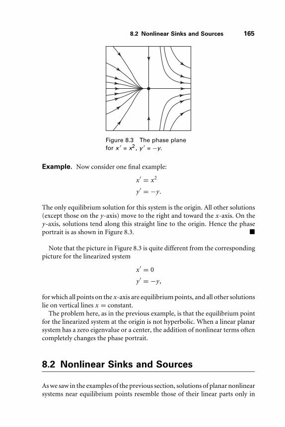
8.2 Nonlinear Sinks and Sources 165
Figure 8.3 The phase planefor x ′ = x2 , y ′ = −y.
Example. Now consider one final example:
x ′ = x2
y ′ = −y .
The only equilibrium solution for this system is the origin. All other solutions(except those on the y-axis) move to the right and toward the x-axis. On they-axis, solutions tend along this straight line to the origin. Hence the phaseportrait is as shown in Figure 8.3. �
Note that the picture in Figure 8.3 is quite different from the correspondingpicture for the linearized system
x ′ = 0
y ′ = −y ,
for which all points on the x-axis are equilibrium points, and all other solutionslie on vertical lines x = constant.
The problem here, as in the previous example, is that the equilibrium pointfor the linearized system at the origin is not hyperbolic. When a linear planarsystem has a zero eigenvalue or a center, the addition of nonlinear terms oftencompletely changes the phase portrait.
8.2 Nonlinear Sinks and Sources
As we saw in the examples of the previous section, solutions of planar nonlinearsystems near equilibrium points resemble those of their linear parts only in

166 Chapter 8 Equilibria in Nonlinear Systems
the case where the linearized system is hyperbolic; that is, when neither ofthe eigenvalues of the system has zero real part. In this section we begin todescribe the situation in the general case of a hyperbolic equilibrium point ina nonlinear system by considering the special case of a sink. For simplicity, wewill prove the results below in the planar case, although all of the results holdin Rn .
Let X ′ = F(X) and suppose that F(X0) = 0. Let DFX0 denote the Jacobianmatrix of F evaluated at X0. Then, as in Chapter 7, the linear system ofdifferential equations
Y ′ = DFX0Y
is called the linearized system near X0. Note that, if X0 = 0, the linearizedsystem is obtained by simply dropping all of the nonlinear terms in F , just aswe did in the previous section.
In analogy with our work with linear systems, we say that an equilibriumpoint X0 of a nonlinear system is hyperbolic if all of the eigenvalues of DFX0
have nonzero real parts.We now specialize the discussion to the case of an equilibrium of a planar
system for which the linearized system has a sink at 0. Suppose our system is
x ′ = f (x , y)
y ′ = g (x , y)
with f (x0, y0) = 0 = g (x0, y0). If we make the change of coordinates u =x − x0, v = y − y0 then the new system has an equilibrium point at (0, 0).Hence we may as well assume that x0 = y0 = 0 at the outset. We thenmake a further linear change of coordinates that puts the linearized systemin canonical form. For simplicity, let us assume at first that the linearizedsystem has distinct eigenvalues −λ < −μ < 0. Thus after these changes ofcoordinates, our system become
x ′ = −λx + h1(x , y)
y ′ = −μy + h2(x , y)
where hj = hj(x , y) contains all of the “higher order terms.” That is, in termsof its Taylor expansion, each hj contains terms that are quadratic or higherorder in x and/or y . Equivalently, we have
lim(x ,y)→(0,0)
hj(x , y)
r= 0
where r2 = x2 + y2.

8.2 Nonlinear Sinks and Sources 167
The linearized system is now given by
x ′ = −λx
y ′ = −μy .
For this linearized system, recall that the vector field always points inside thecircle of radius r centered at the origin. Indeed, if we take the dot product ofthe linear vector field with the outward normal vector (x , y), we find
(−λx , −μy) · (x , y) = −λx2 − μy2 < 0
for any nonzero vector (x , y). As we saw in Chapter 4, this forces all solutionsto tend to the origin with strictly decreasing radial components.
The same thing happens for the nonlinear system, at least close to (0, 0). Letq(x , y) denote the dot product of the vector field with (x , y). We have
q(x , y) = (−λx + h1(x , y), −μy + h2(x , y)) · (x , y)
= −λx2 + xh1(x , y) − μy2 + yh2(x , y)
= −μ(x2 + y2) + (μ − λ)x2 + xh1(x , y) + yh2(x , y)
≤ −μr2 + xh1(x , y) + yh2(x , y)
since (μ − λ)x2 ≤ 0. Therefore we have
q(x , y)
r2≤ −μ + xh1(x , y) + yh2(x , y)
r2.
As r → 0, the right-hand side tends to −μ. Thus it follows that q(x , y) isnegative, at least close to the origin. As a consequence, the nonlinear vectorfield points into the interior of circles of small radius about 0, and so allsolutions whose initial conditions lie inside these circles must tend to theorigin. Thus we are justified in calling this type of equilibrium point a sink,just as in the linear case.
It is straightforward to check that the same result holds if the linearized sys-tem has eigenvalues α+ iβ with α < 0, β �= 0. In the case of repeated negativeeigenvalues, we first need to change coordinates so that the linearized system is
x ′ = −λx + εy
y ′ = −λy
where ε is sufficiently small. We showed how to do this in Chapter 4. Thenagain the vector field points inside circles of sufficiently small radius.

168 Chapter 8 Equilibria in Nonlinear Systems
We can now conjugate the flow of a nonlinear system near a hyperbolicequilibrium point that is a sink to the flow of its linearized system. Indeed,the argument used in the second example of the previous section goes overessentially unchanged. In similar fashion, nonlinear systems near a hyperbolicsource are also conjugate to the corresponding linearized system.
This result is a special case of the following more general theorem.
The Linearization Theorem. Suppose the n-dimensional system X ′ =F(X) has an equilibrium point at X0 that is hyperbolic. Then the nonlinearflow is conjugate to the flow of the linearized system in a neighborhood of X0. �
We will not prove this theorem here, since the proof requires analyticaltechniques beyond the scope of this book when there are eigenvalues presentwith both positive and negative real parts.
8.3 Saddles
We turn now to the case of an equilibrium for which the linearized system hasa saddle at the origin in R2. As in the previous section, we may assume thatthis system is in the form
x ′ = λx + f1(x , y)
y ′ = −μy + f2(x , y)
where −μ < 0 < λ and fj(x , y)/r tends to 0 as r → 0. As in the case of a linearsystem, we call this type of equilibrium point a saddle.
For the linearized system, the y-axis serves as the stable line, with all solutionson this line tending to 0 as t → ∞. Similarly, the x-axis is the unstable line.As we saw in Section 8.1, we cannot expect these stable and unstable straightlines to persist in the nonlinear case. However, there do exist a pair of curvesthrough the origin that have similar properties.
Let W s(0) denote the set of initial conditions whose solutions tend to theorigin as t → ∞. Let W u(0) denote the set of points whose solutions tendto the origin as t → −∞. W s(0) and W u(0) are called the stable curve andunstable curve, respectively.
The following theorem shows that solutions near nonlinear saddles behavemuch the same as in the linear case.
The Stable Curve Theorem. Suppose the system
x ′ = λx + f1(x , y)
y ′ = −μy + f2(x , y)

8.3 Saddles 169
satisfies −μ < 0 < λ and fj(x , y)/r → 0 as r → 0. Then there is an ε > 0and a curve x = hs(y) that is defined for |y| < ε and satisfies hs(0) = 0.Furthermore:
1. All solutions whose initial conditions lie on this curve remain on this curvefor all t ≥ 0 and tend to the origin as t → ∞;
2. The curve x = hs(y) passes through the origin tangent to the y-axis;3. All other solutions whose initial conditions lie in the disk of radius ε centered
at the origin leave this disk as time increases. �Some remarks are in order. The curve x = hs(y) is called the local stable curve
at 0. We can find the complete stable curve W s(0) by following solutions thatlie on the local stable curve backward in time. The function hs(y) is actuallyC∞ at all points, though we will not prove this result here.
A similar unstable curve theorem provides us with a local unstable curveof the form y = hu(x). This curve is tangent to the x-axis at the origin. Allsolutions on this curve tend to the origin as t → −∞.
We begin with a brief sketch of the proof of the stable curve theorem.Consider the square bounded by the lines |x| = ε and |y| = ε for ε > 0sufficiently small. The nonlinear vector field points into the square along theinterior of the top and the bottom boundaries y = ±ε since the system isclose to the linear system x ′ = λx , y ′ = −μy , which clearly has this property.Similarly, the vector field points outside the square along the left and rightboundaries x = ±ε.
Now consider the initial conditions that lie along the top boundary y = ε.Some of these solutions will exit the square to the left, while others will exit tothe right. Solutions cannot do both, so these sets are disjoint. Moreover, thesesets are open. So there must be some initial conditions whose solutions do notexit at all. We will show first of all that each of these nonexiting solutions tendsto the origin. Secondly, we will show that there is only one initial conditionon the top and bottom boundary whose solution behaves in this way. Finallywe will show that this solution lies along some graph of the form x = hs(y),which has the required properties.
Now we fill in the details of the proof. Let Bε denote the square boundedby x = ±ε and y = ±ε. Let S±
ε denote the top and bottom boundaries ofBε . Let CM denote the conical region given by |y| ≥ M |x| inside Bε . Here wethink of the slopes ±M of the boundary of CM as being large in absolute value.See Figure 8.4.
Lemma. Given M > 0, there exists ε > 0 such that the vector field points outsideCM for points on the boundary of CM ∩ Bε (except, of course, at the origin).
Proof: Given M , choose ε > 0 so that
|f1(x , y)| ≤ λ
2√
M 2 + 1r

170 Chapter 8 Equilibria in Nonlinear Systems
x
y
y�Mx
Figure 8.4 The cone CM.
for all (x , y) ∈ Bε . Now suppose x > 0. Then along the right boundary of CM
we have
x ′ = λx + f1(x , Mx)
≥ λx − |f1(x , Mx)|≥ λx − λ
2√
M 2 + 1r
= λx − λ
2√
M 2 + 1(x
√M 2 + 1)
= λ
2x > 0.
Hence x ′ > 0 on this side of the boundary of the cone.Similarly, if y > 0, we may choose ε > 0 smaller if necessary so that we have
y ′ < 0 on the edges of CM where y > 0. Indeed, choosing ε so that
|f2(x , y)| ≤ μ
2√
M 2 + 1r
guarantees this exactly as above. Hence on the edge of CM that lies in the firstquadrant, we have shown that the vector field points down and to the rightand hence out of CM . Similar calculations show that the vector field pointsoutside CM on all other edges of CM . This proves the lemma. �
It follows from this lemma that there is a set of initial conditions in S±ε ∩CM
whose solutions eventually exit from CM to the right, and another set inS±ε ∩ CM whose solutions exit left. These sets are open because of continuity
of solutions with respect to initial conditions (see Section 7.3). We next showthat each of these sets is actually a single open interval.

8.3 Saddles 171
Let C+M denote the portion of CM lying above the x-axis, and let C−
M denotethe portion lying below this axis.
Lemma. Suppose M > 1. Then there is an ε > 0 such that y ′ < 0 in C+M and
y ′ > 0 in C−M .
Proof: In C+M we have |Mx| ≤ y so that
r2 ≤ y2
M 2+ y2
or
r ≤ y
M
√1 + M 2.
As in the previous lemma, we choose ε so that
|f2(x , y)| ≤ μ
2√
M 2 + 1r
for all (x , y) ∈ Bε . We then have in C+M
y ′ ≤ −μy + |f2(x , y)|≤ −μy + μ
2√
M 2 + 1r
≤ −μy + μ
2My
≤ −μ
2y
since M > 1. This proves the result for C+M ; the proof for C−
M is similar. �
From this result we see that solutions that begin on S+ε ∩CM decrease in the
y-direction while they remain in C+M . In particular, no solution can remain in
C+M for all time unless that solution tends to the origin. By the existence and
uniqueness theorem, the set of points in S+ε that exit to the right (or left) must
then be a single open interval. The complement of these two intervals in S+ε is
therefore a nonempty closed interval on which solutions do not leave CM andtherefore tend to 0 as t → ∞. We have similar behavior in C−
M .We now claim that the interval of initial conditions in S±
ε whose solutionstend to 0 is actually a single point. To see this, recall the variational equation

172 Chapter 8 Equilibria in Nonlinear Systems
for this system discussed in Section 7.4. This is the nonautonomous linearsystem
U ′ = DFX(t )U
where X(t ) is a given solution of the nonlinear system and
F
(xy
)=
(λx + f1(x , y)
−μy + f2(x , y)
).
We showed in Chapter 7 that, given τ > 0, if |U0| is sufficiently small, thenthe solution of the variational equation U (t ) that satisfies U (0) = U0 and thesolution Y (t ) of the nonlinear system satisfying Y (0) = X0 + U0 remain closeto each other for 0 ≤ t ≤ τ .
Now let X(t ) = (x(t ), y(t )) be one of the solutions of the system that neverleaves CM . Suppose x(0) = x0 and y(0) = ε.
Lemma. Let U (t ) = (u1(t ), u2(t )) be any solution of the variational equation
U ′ = DFX(t )U
that satisfies |u2(0)/u1(0)| ≤ 1. Then we may choose ε > 0 sufficiently small sothat |u2(t )| ≤ |u1(t )| for all t ≥ 0.
Proof: The variational equation may be written
u′1 = λu1 + f11u1 + f12u2
u′2 = −μu2 + f21u1 + f22u2
where the |fij(t )| may be made as small as we like by choosing ε smaller.Given any solution (u1(t ), u2(t )) of this equation, let η = η(t ) be the slopeu2(t )/u1(t ) of this solution. Using the variational equation and the quotientrule, we find that η satisfies
η′ = α(t ) − (μ + λ + β(t ))η + γ (t )η2
where α(t ) = f21(t ), β(t ) = f11(t )− f22(t ), and γ (t ) = −f12(t ). In particular,α, β, and γ are all small. Recall that μ + λ > 0, so that
−(μ + λ + β(t )) < 0.
It follows that, if η(t ) > 0, there are constants a1 and a2 with 0 < a1 < a2 suchthat
−a2η + α(t ) ≤ η′ ≤ −a1η + α(t ).
Now, if we choose ε small enough and set u1(0) = u2(0) so that η(0) = 1,then we have η′(0) < 0 so that η(t ) initially decreases. Arguing similarly,

8.3 Saddles 173
if η(0) = −1, then η′(0) > 0 so η(t ) increases. In particular, any solutionthat begins with |η(0)| < 1 can never satisfy η(t ) = ±1. Since our solutionsatisfies |η(0)| ≤ 1, it follows that this solution is trapped in the region where|η(t )| < 1, and so we have |u2(t )| ≤ |u1(t )| for all t > 0. This proves thelemma. �
To complete the proof of the theorem, suppose that we have a secondsolution Y (t ) that lies in CM for all time. So Y (t ) → 0 as t → ∞. Supposethat Y (0) = (x ′
0, ε) where x ′0 �= x0. Note that any solution with initial value
(x , ε) with x0 < x < x ′0 must also tend to the origin, so we may assume that
x ′0 is as close as we like to x0. We will approximate Y (t ) − X(t ) by a solution
of the variational equation. Let U (t ) denote the solution of the variationalequation
U ′ = DFX(t )U
satisfying u1(0) = x ′0 − x0, u2(0) = 0. The above lemma applies to U (t ) so
that |u2(t )| ≤ |u1(t )| for all t .We have
|u′1| = |λu1 + f11(t )u1 + f12(t )u2|
≥ λ|u1| − (|f11(t )| + |f12(t )|)|u1|.
But |f11 + f12| tends to 0 as ε → 0, so we have
|u′1| ≥ K |u1|
for some K > 0. Hence |u1(t )| ≥ CeKt for t ≥ 0. Now the solution Y (t ) tendsto 0 by assumption. But then the distance between Y (t ) and U (t ) must becomelarge if u1(0) �= 0. This yields a contradiction and shows that Y (t ) = X(t ).
We finally claim that X(t ) tends to the origin tangentially to the y-axis. Thisfollows immediately from the fact that we may choose ε small enough so thatX(t ) lies in CM no matter how large M is. Hence the slope of X(t ) tends to±∞ as X(t ) approaches (0, 0). �
We conclude this section with a brief discussion of higher dimensionalsaddles. Suppose X ′ = F(X) where X ∈ Rn . Suppose that X0 is an equilibriumsolution for which the linearized system has k eigenvalues with negative realparts and n − k eigenvalues with positive real parts. Then the local stableand unstable sets are not generally curves. Rather, they are “submanifolds” ofdimension k and n − k, respectively. Without entering the realm of manifold

174 Chapter 8 Equilibria in Nonlinear Systems
theory, we simply note that this means there is a linear change of coordinatesin which the local stable set is given near the origin by the graph of a C∞function g : Br → Rn−k that satisfies g (0) = 0, and all partial derivatives of gvanish at the origin. Here Br is the disk of radius r centered at the origin in Rk .The local unstable set is a similar graph over an n − k-dimensional disk. Eachof these graphs is tangent at the equilibrium point to the stable and unstablesubspaces at X0. Hence they meet only at X0.
Example. Consider the system
x ′ = −x
y ′ = −y
z ′ = z + x2 + y2.
The linearized system at the origin has eigenvalues 1 and −1 (repeated). Thechange of coordinates
u = x
v = y
w = z + 1
3(x2 + y2).
converts the nonlinear system to the linear system
u′ = −u
v ′ = −v
w ′ = w .
The plane w = 0 for the linear system is the stable plane. Under the change ofcoordinates this plane is transformed to the surface
z = −1
3(x2 + y2),
which is a paraboloid passing through the origin in R3 and opening downward.All solutions tend to the origin on this surface; we call this the stable surfacefor the nonlinear system. See Figure 8.5. �
8.4 Stability
The study of equilibria plays a central role in ordinary differential equationsand their applications. An equilibrium point, however, must satisfy a certain

8.4 Stability 175
y
x
z�Wu(0)
Ws(0)
Figure 8.5 The phase portraitfor x ′ = −x, y ′ = −y, z ′ =z + x2 + y2 .
stability criterion in order to be significant physically. (Here, as in several otherplaces in this book, we use the word physical in a broad sense; in some contexts,physical could be replaced by biological , chemical , or even economic .)
An equilibrium is said to be stable if nearby solutions stay nearby for allfuture time. In applications of dynamical systems one cannot usually pinpointpositions exactly, but only approximately, so an equilibrium must be stable tobe physically meaningful.
More precisely, suppose X∗ ∈ Rn is an equilibrium point for the differentialequation
X ′ = F(X).
Then X∗ is a stable equilibrium if for every neighborhood O of X∗ in Rn thereis a neighborhood O1 of X∗ in O such that every solution X(t ) with X(0) = X0
in O1 is defined and remains in O for all t > 0.A different form of stability is asymptotic stability. If O1 can be chosen above
so that, in addition to the properties for stability, we have limt→∞ X(t ) = X∗,then we say that X∗ is asymptotically stable.
An equilibrium X∗ that is not stable is called unstable. This means there is aneighborhood O of X∗ such that for every neighborhood O1 of X∗ in O, thereis at least one solution X(t ) starting at X(0) ∈ O1 that does not lie entirely inO for all t > 0.
A sink is asymptotically stable and therefore stable. Sources and saddlesare examples of unstable equilibria. An example of an equilibrium that isstable but not asymptotically stable is the origin in R2 for a linear equationX ′ = AX where A has pure imaginary eigenvalues. The importance of thisexample in applications is limited (despite the famed harmonic oscillator)because the slightest nonlinear perturbation will destroy its character, as we

176 Chapter 8 Equilibria in Nonlinear Systems
saw in Section 8.1. Even a small linear perturbation can make a center into asink or a source.
Thus when the linearization of the system at an equilibrium point is hyper-bolic, we can immediately determine the stability of that point. Unfortunately,many important equilibrium points that arise in applications are nonhyper-bolic. It would be wonderful to have a technique that determined the stabilityof an equilibrium point that works in all cases. Unfortunately, as yet, we haveno universal way of determining stability except by actually finding all solu-tions of the system, which is usually difficult if not impossible. We will presentsome techniques that allow us to determine stability in certain special cases inthe next chapter.
8.5 Bifurcations
In this section we will describe some simple examples of bifurcations that occurfor nonlinear systems. We consider a family of systems
X ′ = Fa(X)
where a is a real parameter. We assume that Fa depends on a in a C∞ fashion.A bifurcation occurs when there is a “significant” change in the structure ofthe solutions of the system as a varies. The simplest types of bifurcations occurwhen the number of equilibrium solutions changes as a varies.
Recall the elementary bifurcations we encountered in Chapter 1 for first-order equations x ′ = fa(x). If x0 is an equilibrium point, then we have fa(x0) =0. If f ′
a (x0) �= 0, then small changes in a do not change the local structure nearx0: that is, the differential equation
x ′ = fa+ε(x)
has an equilibrium point x0(ε) that varies continuously with ε for ε small.A glance at the (increasing or decreasing) graphs of fa+ε(x) near x0 showswhy this is true. More rigorously, this is an immediate consequence of theimplicit function theorem (see Exercise 3 at the end of this chapter). Thusbifurcations for first-order equations only occur in the nonhyperbolic casewhere f ′
a (x0) = 0.
Example. The first-order equation
x ′ = fa(x) = x2 + a

8.5 Bifurcations 177
has a single equilibrium point at x = 0 when a = 0. Note f ′0 (0) = 0, but
f ′′0 (0) �= 0. For a > 0 this equation has no equilibrium points since fa(x) > 0for all x , but for a < 0 this equation has a pair of equilibria. Thus a bifurcationoccurs as the parameter passes through a = 0. �
This kind of bifurcation is called a saddle-node bifurcation (we will see the“saddle” in this bifurcation a little later). In a saddle-node bifurcation, there isan interval about the bifurcation value a0 and another interval I on the x-axisin which the differential equation has
1. Two equilibrium points in I if a < a0;2. One equilibrium point in I if a = a0;3. No equilibrium points in I if a > a0.
Of course, the bifurcation could take place “the other way,” with no equilibriawhen a > a0. The example above is actually the typical type of bifurcation forfirst-order equations.
Theorem. (Saddle-Node Bifurcation) Suppose x ′ = fa(x) is a first-orderdifferential equation for which
1. fa0(x0) = 0;
2. f ′a0
(x0) = 0;
3. f ′′a0
(x0) �= 0;
4.∂fa0
∂a(x0) �= 0.
Then this differential equation undergoes a saddle-node bifurcation at a = a0.
Proof: Let G(x , a) = fa(x). We have G(x0, a0) = 0. Also,
∂G
∂a(x0, a0) = ∂fa0
∂a(x0) �= 0,
so we may apply the implicit function theorem to conclude that there is asmooth function a = a(x) such that G(x , a(x)) = 0. In particular, if x∗belongs to the domain of a(x), then x∗ is an equilibrium point for the equationx ′ = fa(x∗)(x), since fa(x∗)(x
∗) = 0. Differentiating G(x , a(x)) = 0 withrespect to x , we find
a′(x) = −∂G/∂x
∂G/∂a.

178 Chapter 8 Equilibria in Nonlinear Systems
Now (∂G/∂x)(x0, a0) = f ′a0
(x0) = 0, while (∂G/∂a)(x0, a0) �= 0 by assump-tion. Hence a′(x0) = 0. Differentiating once more, we find
a′′(x) =−∂2G
∂x2
∂G
∂a+ ∂G
∂x
∂2G
∂a2(∂G
∂a
)2 .
Since (∂G/∂x)(x0, a0) = 0, we have
a′′(x0) =−∂2G
∂x2(x0, a0)
∂G
∂a(x0, a0)
�= 0
since (∂2G/∂x2)(x0, a0) = f ′′a0
(x0) �= 0. This implies that the graph of a = a(x)is either concave up or concave down, so we have two equilibria near x0 fora-values on one side of a0 and no equilibria for a-values on the other side. �
We said earlier that such saddle-node bifurcations were the “typical” bifur-cations involving equilibrium points for first-order equations. The reason forthis is that we must have both
1. fa0(x0) = 02. f ′
a0(x0) = 0
if x ′ = fa(x) is to undergo a bifurcation when a = a0. Generically (in the senseof Section 5.6), the next higher order derivatives at (x0, a0) will be nonzero.That is, we typically have
3. f ′′a0
(x0) �= 0
4. ∂fa∂a (x0, a0) �= 0
at such a bifurcation point. But these are precisely the conditions that guaranteea saddle-node bifurcation.
Recall that the bifurcation diagram for x ′ = fa(x) is a plot of the variousphase lines of the equation versus the parameter a. The bifurcation diagramfor a typical saddle-node bifurcation is displayed in Figure 8.6. (The directionsof the arrows and the curve of equilibria may change.)
Example. (Pitchfork Bifurcation) Consider
x ′ = x3 − ax .

8.5 Bifurcations 179
x
a0
x0
a
Figure 8.6 The bifurcation diagram for asaddle-node bifurcation.
x
a
Figure 8.7 The bifurcation diagramfor a pitchfork bifurcation.
There are three equilibria for this equation, at x = 0 and x = ±√a when
a > 0. When a ≤ 0, x = 0 is the only equilibrium point. The bifurcationdiagram shown in Figure 8.7 explains why this bifurcation is so named. �
Now we turn to some bifurcations in higher dimensions. The saddle-nodebifurcation in the plane is similar to its one-dimensional cousin, only now wesee where the “saddle” comes from.
Example. Consider the system
x ′ = x2 + a
y ′ = −y .

180 Chapter 8 Equilibria in Nonlinear Systems
Figure 8.8 The saddle-node bifurcation when, from left to right,a < 0, a = 0, and a > 0.
When a = 0, this is one of the systems considered in Section 8.1. There is aunique equilibrium point at the origin, and the linearized system has a zeroeigenvalue.
When a passes through a = 0, a saddle-node bifurcation occurs. Whena > 0, we have x ′ > 0 so all solutions move to the right; the equilibrium pointdisappears. When a < 0 we have a pair of equilibria, at the points (±√−a, 0).The linearized equation is
X ′ =(
2x 00 −1
)X .
So we have a sink at (−√−a, 0) and a saddle at (√−a, 0). Note that solutions
on the lines x = ±√−a remain for all time on these lines since x ′ = 0 on theselines. Solutions tend directly to the equilibria on these lines since y ′ = −y .This bifurcation is sketched in Figure 8.8. �
A saddle-node bifurcation may have serious global implications for thebehavior of solutions, as the following example shows.
Example. Consider the system given in polar coordinates by
r ′ = r − r3
θ ′ = sin2(θ) + a
where a is again a parameter. The origin is always an equilibrium point sincer ′ = 0 when r = 0. There are no other equilibria when a > 0 since, in thatcase, θ ′ > 0. When a = 0 two additional equilibria appear at (r , θ) = (1, 0)and (r , θ) = (1, π). When −1 < a < 0, there are four equilibria on the circler = 1. These occur at the roots of the equation
sin2(θ) = −a.

8.5 Bifurcations 181
We denote these roots by θ± and θ± + π , where we assume that 0 < θ+ < π /2and −π /2 < θ− < 0.
Note that the flow of this system takes the straight rays through the originθ = constant to other straight rays. This occurs since θ ′ depends only on θ ,not on r . Also, the unit circle is invariant in the sense that any solution thatstarts on the circle remains there for all time. This follows since r ′ = 0 on thiscircle. All other nonzero solutions tend to this circle, since r ′ > 0 if 0 < r < 1whereas r ′ < 0 if r > 1.
Now consider the case a = 0. In this case the x-axis is invariant and allnonzero solutions on this line tend to the equilibrium points at x = ±1. Inthe upper half-plane we have θ ′ > 0, so all other solutions in this region windcounterclockwise about 0 and tend to x = −1; the θ-coordinate increasesto θ = π while r tends monotonically to 1. No solution winds more thanangle π about the origin, since the x-axis acts as a barrier. The system behavessymmetrically in the lower half-plane.
When a > 0 two things happen. First of all, the equilibrium points at x = ±1disappear and now θ ′ > 0 everywhere. Thus the barrier on the x-axis has beenremoved and all solutions suddenly are free to wind forever about the origin.Secondly, we now have a periodic solution on the circle r = 1, and all nonzerosolutions are attracted to it.
This dramatic change is caused by a pair of saddle-node bifurcations ata = 0. Indeed, when −1 < a < 0 we have two pair of equilibria on the unitcircle. The rays θ = θ± and θ = θ± + π are invariant, and all solutionson these rays tend to the equilibria on the circle. Consider the half-planeθ− < θ < θ− + π . For θ-values in the interval θ− < θ < θ+, we have θ ′ < 0,while θ ′ > 0 in the interval θ+ < θ < θ− + π . Solutions behave symmetricallyin the complementary half-plane. Therefore all solutions that do not lie on therays θ = θ+ or θ = θ+ + π tend to the equilibrium points at r = 1, θ = θ−or at r = 1, θ = θ− + π . These equilibria are therefore sinks. At the otherequilibria we have saddles. The stable curves of these saddles lie on the raysθ = θ+ and θ = π + θ+ and the unstable curves of the saddles are given bythe unit circle minus the sinks. See Figure 8.9. �
The previous examples all featured bifurcations that occur when the lin-earized system has a zero eigenvalue. Another case where the linearized systemfails to be hyperbolic occurs when the system has pure imaginary eigenvalues.
Example. (Hopf Bifurcation) Consider the system
x ′ = ax − y − x(x2 + y2)
y ′ = x + ay − y(x2 + y2).

182 Chapter 8 Equilibria in Nonlinear Systems
Figure 8.9 Global effects of saddle-node bifurcations when, from leftto right, a < 0, a = 0, and a > 0.
There is an equilibrium point at the origin and the linearized system is
X ′ =(
a −11 a
)X .
The eigenvalues are a ± i, so we expect a bifurcation when a = 0.To see what happens as a passes through 0, we change to polar coordinates.
The system becomes
r ′ = ar − r3
θ ′ = 1.
Note that the origin is the only equilibrium point for this system, since θ ′ �= 0.For a < 0 the origin is a sink since ar − r3 < 0 for all r > 0. Thus all solutionstend to the origin in this case. When a > 0, the equilibrium becomes a source.So what else happens? When a > 0 we have r ′ = 0 if r = √
a. So the circleof radius
√a is a periodic solution with period 2π . We also have r ′ > 0 if
0 < r <√
a, while r ′ < 0 if r >√
a. Thus, all nonzero solutions spiral towardthis circular solution as t → ∞.
This type of bifurcation is called a Hopf bifurcation. Thus at a Hopfbifurcation, no new equilibria arise. Instead, a periodic solution is bornat the equilibrium point as a passes through the bifurcation value. SeeFigure 8.10. �
8.6 Exploration: Complex Vector Fields
In this exploration, you will investigate the behavior of systems of differentialequations in the complex plane of the form z ′ = F(z). Throughout thissection z will denote the complex number z = x + iy and F(z) will be a

8.6 Exploration: Complex Vector Fields 183
Figure 8.10 The Hopf bifurcation for a < 0 anda > 0.
polynomial with complex coefficients. Solutions of the differential equationwill be expressed as curves z(t ) = x(t ) + iy(t ) in the complex plane.
You should be familiar with complex functions such as the exponential, sine,and cosine as well as with the process of taking complex square roots in orderto comprehend fully what you see below. Theoretically, you should also havea grasp of complex analysis as well. However, all of the routine tricks fromintegration of functions of real variables work just as well when integratingwith respect to z . You need not prove this, because you can always check thevalidity of your solutions when you have completed the integrals.
1. Solve the equation z ′ = az where a is a complex number. What kindof equilibrium points do you find at the origin for these differentialequations?
2. Solve each of the following complex differential equations and sketch thephase portrait.
(a) z ′ = z2
(b) z ′ = z2 − 1
(c) z ′ = z2 + 1
3. For a complex polynomial F(z), the complex derivative is defined just asthe real derivative
F ′(z0) = limz→z0
F(z) − F(z0)
z − z0,
only this limit is evaluated along any smooth curve in C that passesthrough z0. This limit must exist and yield the same (complex) numberfor each such curve. For polynomials, this is easily checked. Now write
F(x + iy) = u(x , y) + iv(x , y).

184 Chapter 8 Equilibria in Nonlinear Systems
Evaluate F ′(z0) in terms of the derivatives of u and v by first taking thelimit along the horizontal line z0 + t , and secondly along the vertical linez0+it . Use this to conclude that, if the derivative exists, then we must have
∂u
∂x= ∂v
∂yand
∂u
∂y= −∂v
∂x
at every point in the plane. The equations are called the Cauchy-Riemannequations.
4. Use the above observation to determine all possible types of equilibriumpoints for complex vector fields.
5. Solve the equation
z ′ = (z − z0)(z − z1)
where z0, z1 ∈ C, and z0 �= z1. What types of equilibrium points occurfor different values of z0 and z1?
6. Find a nonlinear change of variables that converts the previous system tow ′ = αw with α ∈ C. Hint: Since the original system has two equilibriumpoints and the linear system only one, the change of variables must sendone of the equilibrium points to ∞.
7. Classify all complex quadratic systems of the form
z ′ = z2 + az + b
where a, b ∈ C.8. Consider the equation
z ′ = z3 + az
with a ∈ C. First use a computer to describe the phase portraits for thesesystems. Then prove as much as you can about these systems and classifythem with respect to a.
9. Choose your own (nontrivial) family of complex functions depending ona parameter a ∈ C and provide a complete analysis of the phase por-traits for each a. Some neat families to consider include a exp z , a sin z ,or (z2 + a)(z2 − a).
E X E R C I S E S
1. For each of the following nonlinear systems,
(a) Find all of the equilibrium points and describe the behavior of theassociated linearized system.

Exercises 185
(b) Describe the phase portrait for the nonlinear system.
(c) Does the linearized system accurately describe the local behaviornear the equilibrium points?
(i) x ′ = sin x , y ′ = cos y(ii) x ′ = x(x2 + y2), y ′ = y(x2 + y2)(iii) x ′ = x + y2, y ′ = 2y(iv) x ′ = y2, y ′ = y(v) x ′ = x2, y ′ = y2
2. Find a global change of coordinates that linearizes the system
x ′ = x + y2
y ′ = −y
z ′ = −z + y2.
3. Consider a first-order differential equation
x ′ = fa(x)
for which fa(x0) = 0 and f ′a (x0) �= 0. Prove that the differential equation
x ′ = fa+ε(x)
has an equilibrium point x0(ε) where ε → x0(ε) is a smooth functionsatisfying x0(0) = x0 for ε sufficiently small.
4. Find general conditions on the derivatives of fa(x) so that the equation
x ′ = fa(x)
undergoes a pitchfork bifurcation at a = a0. Prove that your conditionslead to such a bifurcation.
5. Consider the system
x ′ = x2 + y
y ′ = x − y + a
where a is a parameter.
(a) Find all equilibrium points and compute the linearized equation ateach.
(b) Describe the behavior of the linearized system at each equilibriumpoint.

186 Chapter 8 Equilibria in Nonlinear Systems
(c) Describe any bifurcations that occur.
6. Given an example of a family of differential equations x ′ = fa(x) forwhich there are no equilibrium points if a < 0; a single equilibrium ifa = 0; and four equilibrium points if a > 0. Sketch the bifurcationdiagram for this family.
7. Discuss the local and global behavior of solutions of
r ′ = r − r3
θ ′ = sin2(θ) + a
at the bifurcation value a = −1.8. Discuss the local and global behavior of solutions of
r ′ = r − r2
θ ′ = sin2(θ /2) + a
at all of the bifurcation values.9. Consider the system
r ′ = r − r2
θ ′ = sin θ + a
(a) For which values of a does this system undergo a bifurcation?
(b) Describe the local behavior of solutions near the bifurcation values(at, before, and after the bifurcation).
(c) Sketch the phase portrait of the system for all possible different cases.
(d) Discuss any global changes that occur at the bifurcations.
10. Let X ′ = F(X) be a nonlinear system in Rn . Suppose that F(0) = 0 andthat DF0 has n distinct eigenvalues with negative real parts. Describe theconstruction of a conjugacy between this system and its linearization.
11. Consider the system X ′ = F(X) where X ∈ Rn . Suppose that F has anequilibrium point at X0. Show that there is a change of coordinates thatmoves X0 to the origin and converts the system to
X ′ = AX + G(X)
where A is an n × n matrix, which is the canonical form of DFX0 andwhere G(X) satisfies
lim|X |→0
|G(X)||X | = 0.

Exercises 187
12. In the definition of an asymptotically stable equilibrium point, werequired that the equilibrium point also be stable. This requirement isnot vacuous. Give an example of a phase portrait (a sketch is sufficient)that has an equilibrium point toward which all nearby solution curves(eventually) tend, but that is not stable.

This Page Intentionally Left Blank
9Global Nonlinear Techniques
In this chapter we present a variety of qualitative techniques for analyzingthe behavior of nonlinear systems of differential equations. The reader shouldbe forewarned that none of these techniques works for all nonlinear systems;most work only in specialized situations, which, as we shall see in the ensuingchapters, nonetheless occur in many important applications of differentialequations.
9.1 Nullclines
One of the most useful tools for analyzing nonlinear systems of differentialequations (especially planar systems) are the nullclines. For a system in theform
x ′1 = f1(x1, . . . , xn)
...
x ′n = fn(x1, . . . , xn),
the xj-nullcline is the set of points where x ′j vanishes, so the xj-nullcline is the
set of points determined by setting fj(x1, . . . , xn) = 0.The xj-nullclines usually separate Rn into a collection of regions in which
the xj-components of the vector field point in either the positive or negativedirection. If we determine all of the nullclines, then this allows us to decompose
189

190 Chapter 9 Global Nonlinear Techniques
Rn into a collection of open sets, in each of which the vector field points in a“certain direction.”
This is easiest to understand in the case of a planar system
x ′ = f (x , y)
y ′ = g (x , y).
On the x-nullclines, we have x ′ = 0, so the vector field points straight upor down, and these are the only points at which this happens. Therefore thex-nullclines divide R2 into regions where the vector field points either to theleft or to the right. Similarly, on the y-nullclines, the vector field is horizontal,so the y-nullclines separate R2 into regions where the vector field points eitherupward or downward. The intersections of the x- and y-nullclines yield theequilibrium points. In any of the regions between the nullclines, the vector fieldis neither vertical nor horizontal, so it must point in one of four directions:northeast, northwest, southeast, or southwest. We call such regions basicregions. Often, a simple sketch of the basic regions allows us to understand thephase portrait completely, at least from a qualitative point of view.
Example. For the system
x ′ = y − x2
y ′ = x − 2,
the x-nullcline is the parabola y = x2 and the y-nullcline is the vertical line x =2. These nullclines meet at (2, 4) so this is the only equilibrium point. The null-clines divide R2 into four basic regions labeled A through D in Figure 9.1(a).By first choosing one point in each of these regions, and then determining thedirection of the vector field at that point, we can decide the direction of thevector field at all points in the basic region. For example, the point (0, 1) lies inregion A and the vector field is (1, −2) at this point, which points toward thesoutheast. Hence the vector field points southeast at all points in this region.Of course, the vector field may be nearly horizontal or nearly vertical in thisregion; when we say southeast we mean that the angle θ of the vector field liesin the sector −π /2 < θ < 0. Continuing in this fashion we get the directionof the vector field in all four regions, as in Figure 9.1(b). This also determinesthe horizontal and vertical directions of the vector field on the nullclines.
Just from the direction field alone, it appears that the equilibrium point is asaddle. Indeed, this is the case because the linearized system at (2, 4) is
X ′ =(−4 1
1 0
)X ,

9.1 Nullclines 191
A
D C
B
(a) (b)
Figure 9.1 The (a) nullclines and (b) direction field.
y�x2
x�2B
Figure 9.2 Solutionsenter the basic regionB and then tend to ∞.
which has eigenvalues −2 ± √5, one of which is positive, the other negative.
More importantly, we can fill in the approximate behavior of solutionseverywhere in the plane. For example, note that the vector field points into thebasic region marked B at all points along its boundary, and then it points north-easterly at all points inside B. Thus any solution in region B must stay in regionB for all time and tend toward ∞ in the northeast direction. See Figure 9.2.Similarly, solutions in the basic region D stay in that region and head toward∞ in the southwest direction. Solutions starting in the basic regions A andC have a choice: They must eventually cross one of the nullclines and enterregions B and D (and therefore we know their ultimate behavior) or else theytend to the equilibrium point. However, there is only one curve of such solu-tions in each region, the stable curve at (2, 4). Thus we completely understandthe phase portrait for this system, at least from a qualitative point of view. SeeFigure 9.3. �
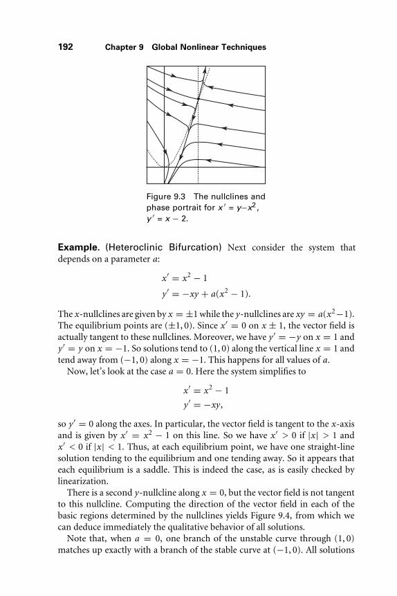
192 Chapter 9 Global Nonlinear Techniques
Figure 9.3 The nullclines andphase portrait for x ′ = y−x2 ,y ′ = x − 2.
Example. (Heteroclinic Bifurcation) Next consider the system thatdepends on a parameter a:
x ′ = x2 − 1
y ′ = −xy + a(x2 − 1).
The x-nullclines are given by x = ±1 while the y-nullclines are xy = a(x2−1).The equilibrium points are (±1, 0). Since x ′ = 0 on x ± 1, the vector field isactually tangent to these nullclines. Moreover, we have y ′ = −y on x = 1 andy ′ = y on x = −1. So solutions tend to (1, 0) along the vertical line x = 1 andtend away from (−1, 0) along x = −1. This happens for all values of a.
Now, let’s look at the case a = 0. Here the system simplifies to
x ′ = x2 − 1
y ′ = −xy ,
so y ′ = 0 along the axes. In particular, the vector field is tangent to the x-axisand is given by x ′ = x2 − 1 on this line. So we have x ′ > 0 if |x| > 1 andx ′ < 0 if |x| < 1. Thus, at each equilibrium point, we have one straight-linesolution tending to the equilibrium and one tending away. So it appears thateach equilibrium is a saddle. This is indeed the case, as is easily checked bylinearization.
There is a second y-nullcline along x = 0, but the vector field is not tangentto this nullcline. Computing the direction of the vector field in each of thebasic regions determined by the nullclines yields Figure 9.4, from which wecan deduce immediately the qualitative behavior of all solutions.
Note that, when a = 0, one branch of the unstable curve through (1, 0)matches up exactly with a branch of the stable curve at (−1, 0). All solutions

9.1 Nullclines 193
(a) (b)
Figure 9.4 The (a) nullclines and (b) phase portrait for x ′ =x2 − 1, y ′ = −xy.
on this curve simply travel from one saddle to the other. Such solutions arecalled heteroclinic solutions or saddle connections. Typically, for planar systems,stable and unstable curves rarely meet to form such heteroclinic “connections.”When they do, however, one can expect a bifurcation.
Now consider the case where a �= 0. The x-nullclines remain the same, atx = ±1. But the y-nullclines change drastically as shown in Figure 9.5. Theyare given by y = a(x2 − 1)/x .
When a > 0, consider the basic region denoted by A. Here the vector fieldpoints southwesterly. In particular, the vector field points in this directionalong the x-axis between x = −1 and x = 1. This breaks the heteroclinicconnection: The right portion of the stable curve associated to (−1, 0) must
(a)
A
A
(b)
Figure 9.5 The (a) nullclines and (b) phase plane when a > 0 afterthe heteroclinic bifurcation.

194 Chapter 9 Global Nonlinear Techniques
now come from y = ∞ in the upper half plane, while the left portion of theunstable curve associated to (1, 0) now descends to y = −∞ in the lowerhalf plane. This opens an “avenue” for certain solutions to travel from y =+∞ to y = −∞ between the two lines x = ±1. Whereas when a = 0 allsolutions remain for all time confined to either the upper or lower half-plane,the heteroclinic bifurcation at a = 0 opens the door for certain solutions tomake this transit.
A similar situation occurs when a < 0 (see Exercise 2 at the end of thischapter). �
9.2 Stability of Equilibria
Determining the stability of an equilibrium point is straightforward if theequilibrium is hyperbolic. When this is not the case, this determinationbecomes more problematic. In this section we develop an alternative methodfor showing that an equilibrium is asymptotically stable. Due to the Russianmathematician Liapunov, this method generalizes the notion that, for a linearsystem in canonical form, the radial component r decreases along solutioncurves. Liapunov noted that other functions besides r could be used for thispurpose. Perhaps more importantly, Liapunov’s method gives us a grasp onthe size of the basin of attraction of an asymptotically stable equilibrium point.By definition, the basin of attraction is the set of all initial conditions whosesolutions tend to the equilibrium point.
Let L : O → R be a differentiable function defined on an open set O in Rn
that contains an equilibrium point X∗ of the system X ′ = F(X). Consider thefunction
L(X) = DLX (F(X)).
As we have seen, if φt (X) is the solution of the system passing through X whent = 0, then we have
L(X) = d
dt
∣∣∣∣t=0
L ◦ φt (X)
by the chain rule. Consequently, if L(X) is negative, then L decreases alongthe solution curve through X .
We can now state Liapunov’s stability theorem:
Theorem. (Liapunov Stability) Let X∗ be an equilibrium point for X ′ =F(X). Let L : O → R be a differentiable function defined on an open set O

9.2 Stability of Equilibria 195
containing X∗. Suppose further that
(a) L(X∗) = 0 and L(X) > 0 if X �= X∗;(b) L ≤ 0 in O − X∗.
Then X∗ is stable. Furthermore, if L also satisfies
(c) L < 0 in O − X∗,
then X∗ is asymptotically stable. �
A function L satisfying (a) and (b) is called a Liapunov function for X∗. If(c) also holds, we call L a strict Liapunov function.
Note that Liapunov’s theorem can be applied without solving the differentialequation; all we need to compute is DLX (F(X)). This is a real plus! On theother hand, there is no cut-and-dried method of finding Liapunov functions; itis usually a matter of ingenuity or trial and error in each case. Sometimes thereare natural functions to try. For example, in the case of mechanical or electricalsystems, energy is often a Liapunov function, as we shall see in Chapter 13.
Example. Consider the system of differential equations in R3 given by
x ′ = (εx + 2y)(z + 1)
y ′ = (−x + εy)(z + 1)
z ′ = −z3
where ε is a parameter. The origin is the only equilibrium point for this system.The linearization of the system at (0, 0, 0) is
Y ′ =⎛⎝ ε 2 0
−1 ε 00 0 0
⎞⎠Y .
The eigenvalues are 0 and ε ±√2i. Hence, from the linearization, we can only
conclude that the origin is unstable if ε > 0. When ε ≤ 0, all we can concludeis that the origin is not hyperbolic.
When ε ≤ 0 we search for a Liapunov function for (0, 0, 0) of the formL(x , y , z) = ax2 + by2 + cz2, with a, b, c > 0. For such an L, we have
L = 2(axx ′ + byy ′ + czz ′),
so that
L/2 = ax(εx + 2y)(z + 1) + by(−x + εy)(z + 1) − cz4
= ε(ax2 + by2)(z + 1) + (2a − b)(xy)(z + 1) − cz4.

196 Chapter 9 Global Nonlinear Techniques
For stability, we want L ≤ 0; this can be arranged, for example, by settinga = 1, b = 2, and c = 1. If ε = 0, we then have L = −z4 ≤ 0, so the originis stable. It can be shown (see Exercise 4) that the origin is not asymptoticallystable in this case.
If ε < 0, then we find
L = ε(x2 + 2y2)(z + 1) − z4
so that L < 0 in the region O given by z > −1 (minus the origin). We concludethat the origin is asymptotically stable in this case, and, indeed, from Exercise 4,that all solutions that start in the region O tend to the origin. �
Example. (The Nonlinear Pendulum) Consider a pendulum consistingof a light rod of length � to which is attached a ball of mass m. The other endof the rod is attached to a wall at a point so that the ball of the pendulummoves on a circle centered at this point. The position of the mass at time tis completely described by the angle θ(t ) of the mass from the straight downposition and measured in the counterclockwise direction. Thus the positionof the mass at time t is given by (� sin θ(t ), −� cos θ(t )).
The speed of the mass is the length of the velocity vector, which is � dθ /dt ,and the acceleration is � d2θ /dt 2. We assume that the only two forces actingon the pendulum are the force of gravity and a force due to friction. Thegravitational force is a constant force equal to mg acting in the downwarddirection; the component of this force tangent to the circle of motion is givenby −mg sin θ . We take the force due to friction to be proportional to velocityand so this force is given by −b� dθ /dt for some constant b > 0. When thereis no force due to friction (b = 0), we have an ideal pendulum. Newton’s lawthen gives the second-order differential equation for the pendulum
m�d2θ
dt 2= −b�
dθ
dt− mg sin θ .
For simplicity, we assume that units have been chosen so that m = � = g = 1.Rewriting this equation as a system, we introduce v = dθ /dt and get
θ ′ = v
v ′ = −bv − sin θ .
Clearly, we have two equilibrium points (mod 2π): the downward rest positionat θ = 0, v = 0, and the straight-up position θ = π , v = 0. This upwardpostion is an unstable equilibrium, both from a mathematical (check thelinearization) and physical point of view.

9.2 Stability of Equilibria 197
For the downward equilibrium point, the linearized system is
Y ′ =(
0 1−1 −b
)Y .
The eigenvalues here are either pure imaginary (when b = 0) or else have neg-ative real parts (when b > 0). So the downward equilibrium is asymptoticallystable if b > 0 as everyone on earth who has watched a real-life pendulumknows.
To investigate this equilibrium point further, consider the functionE(θ , v) = 1
2v2 + 1 − cos θ . For readers with a background in elementarymechanics, this is the well-known total energy function, which we will describefurther in Chapter 13. We compute
E = vv ′ + sin θ θ ′ = −bv2,
so that E ≤ 0. Hence E is a Liapunov function. Thus the origin is a stableequilibrium. If b = 0 (that is, there is no friction), then E ≡ 0. That is, E isconstant along all solutions of the system. Hence we may simply plot the levelcurves of E to see where the solution curves reside. We find the phase portraitshown in Figure 9.6. Note that we do not have to solve the differential equationto paint this picture; knowing the level curves of E (and the direction of thevector field) tells us everything. We will encounter many such (very special)functions that are constant along solution curves later in this chapter.
The solutions encircling the origin have the property that −π < θ(t ) < π
for all t . Therefore these solutions correspond to the pendulum oscillatingabout the downward rest position without ever crossing the upward positionθ = π . The special solutions connecting the equilibrium points at (±π , 0)
2π�2π
Figure 9.6 The phase portrait for theideal pendulum.

198 Chapter 9 Global Nonlinear Techniques
correspond to the pendulum tending to the upward-pointing equilibrium inboth the forward and backward time directions. (You don’t often see suchmotions!) Beyond these special solutions we find solutions for which θ(t )either increases or decreases for all time; in these cases the pendulum spinsforever in the counterclockwise or clockwise direction. �
We will return to the pendulum example for the case b > 0 later, but firstwe prove Liapunov’s theorem.
Proof: Let δ > 0 be so small that the closed ball Bδ(X∗) around the equilib-rium point X∗ of radius δ lies entirely in O. Let α be the minimum value ofL on the boundary of Bδ(X∗), that is, on the sphere Sδ(X∗) of radius δ andcenter X∗. Then α > 0 by assumption. Let U = {X ∈ Bδ(X∗) | L(X) < α}and note that X∗ lies in U . Then no solution starting in U can meet Sδ(X∗)since L is nonincreasing on solution curves. Hence every solution startingin U never leaves Bδ(X∗). This proves that X∗ is stable.
Now suppose that assumption (c) in the Liapunov stability theorem holdsas well, so that L is strictly decreasing on solutions in U − X∗. Let X(t ) bea solution starting in U − X∗ and suppose that X(tn) → Z0 ∈ Bδ(X∗) forsome sequence tn → ∞. We claim that Z0 = X∗. To see this, observe thatL(X(t )) > L(Z0) for all t ≥ 0 since L(X(t )) decreases and L(X(tn)) → L(Z0)by continuity of L. If Z0 �= X∗, let Z (t ) be the solution starting at Z0. Forany s > 0, we have L(Z (s)) < L(Z0). Hence for any solution Y (s) startingsufficiently near Z0 we have
L(Y (s)) < L (Z0) .
Setting Y (0) = X(tn) for sufficiently large n yields the contradiction
L(X (tn + s)) < L (Z0) .
Therefore Z0 = X∗. This proves that X∗ is the only possible limit point of theset {X(t ) | t ≥ 0} and completes the proof of Liapunov’s theorem. �
Figure 9.7 makes the theorem intuitively obvious. The condition L < 0means that when a solution crosses a “level surface” L−1(c), it moves insidethe set where L ≤ c and can never come out again. Unfortunately, it issometimes difficult to justify the diagram shown in this figure; why should thesets L−1(c) shrink down to X∗? Of course, in many cases, Figure 9.7 is indeedcorrect, as, for example, if L is a quadratic function such as ax2 + by2 witha, b > 0. But what if the level surfaces look like those shown in Figure 9.8? Itis hard to imagine such an L that fulfills all the requirements of a Liapunovfunction; but rather than trying to rule out that possibility, it is simpler to givethe analytic proof as above.

9.2 Stability of Equilibria 199
L�1(c2)
L�1(c1)
L�1(c3)
Figure 9.7 Solutions decrease through the level sets L−1(cj)of a strict Liapunov function.
Example. Now consider the system
x ′ = −x3
y ′ = −y(x2 + z2 + 1)
z ′ = − sin z .
The origin is again an equilibrium point. It is not the only one, however,since (0, 0, nπ) is also an equilibrium point for each n ∈ Z. Hence the origincannot be globally asymptotically stable. Moreover, the planes z = nπ forn ∈ Z are invariant in the sense that any solution that starts on one of theseplanes remains there for all time. This occurs since z ′ = 0 when z = nπ . Inparticular, any solution that begins in the region |z | < π must remain trappedin this region for all time.
L�1(c2)L�1(c1)
Figure 9.8 Level sets of a Liapunovfunction may look like this.

200 Chapter 9 Global Nonlinear Techniques
Linearization at the origin yields the system
Y ′ =⎛⎝0 0 0
0 −1 00 0 −1
⎞⎠Y
which tells us nothing about the stability of this equilibrium point.However, consider the function
L(x , y , z) = x2 + y2 + z2.
Clearly, L > 0 except at the origin. We compute
L = −2x4 − 2y2(x2 + z2 + 1) − 2z sin z .
Then L < 0 at all points in the set |z | < π (except the origin) since z sin z > 0when z �= 0. Hence the origin is asymptotically stable.
Moreover, we can conclude that the basin of attraction of the origin is theentire region |z | < π . From the proof of the Liapunov stability theorem, itfollows immediately that any solution that starts inside a sphere of radius r < π
must tend to the origin. Outside of the sphere of radius π and between theplanes z = ±π , the function L is still strictly decreasing. Since solutions aretrapped between these two planes, it follows that they too must tend to theorigin. �
Liapunov functions not only detect stable equilibria; they can also be used toestimate the size of the basin of attraction of an asymptotically stable equilib-rium, as the above example shows. The following theorem gives a criterion forasymptotic stability and the size of the basin even when the Liapunov functionis not strict. To state it, we need several definitions.
Recall that a set P is called invariant if for each X ∈ P , φt (X) is definedand in P for all t ∈ R. For example, the region |z | < π in the above exampleis an invariant set. The set P is positively invariant if for each X ∈ P , φt (X)is defined and in P for all t ≥ 0. The portion of the region |z | < π insidea sphere centered at the origin in the previous example is positively invariantbut not invariant. Finally, an entire solution of a system is a set of the form{φt (X) | t ∈ R}.
Theorem. (Lasalle’s Invariance Principle) Let X∗ be an equilibriumpoint for X ′ = F(X) and let L : U → R be a Liapunov function for X∗, whereU is an open set containing X∗. Let P ⊂ U be a neighborhood of X∗ that is closedand bounded. Suppose that P is positively invariant, and that there is no entiresolution in P − X∗ on which L is constant. Then X∗ is asymptotically stable, andP is contained in the basin of attraction of X∗. �

9.2 Stability of Equilibria 201
Before proving this theorem we apply it to the equilibrium X∗ = (0, 0) ofthe damped pendulum discussed previously. Recall that a Liapunov functionis given by E(θ , v) = 1
2v2 + 1 − cos θ and that E = −bv2. Since E = 0 onv = 0, this Liapunov function is not strict.
To estimate the basin of (0, 0), fix a number c with 0 < c < 2, and define
Pc = {(θ , v) | E(θ , v) ≤ c and |θ | < π}.Clearly, (0, 0) ∈ Pc . We shall prove that Pc lies in the basin of attraction of(0, 0).
Note first that Pc is positively invariant. To see this suppose that (θ(t ), v(t ))is a solution with (θ(0), v(0)) ∈ Pc . We claim that (θ(t ), v(t )) ∈ Pc for allt ≥ 0. We clearly have E(θ(t ), v(t )) ≤ c since E ≤ 0. If |θ(t )| ≥ π , then theremust exist a smallest t0 such that θ(t0) = ±π . But then
E(θ(t0), v(t0)) = E(±π , v(t0))
= 1
2v(t0)2 + 2
≥ 2.
However,
E(θ(t0), v(t0)) ≤ c < 2.
This contradiction shows that θ(t0) < π , and so Pc is positively invariant.We now show that there is no entire solution in Pc on which E is constant
(except the equilibrium solution). Suppose there is such a solution. Then,along that solution, E ≡ 0 and so v ≡ 0. Hence, θ ′ = 0 so θ is constant onthe solution. We also have v ′ = − sin θ = 0 on the solution. Since |θ | < π , itfollows that θ ≡ 0. Thus the only entire solution in Pc on which E is constantis the equilibrium point (0, 0).
Finally, Pc is a closed set. Because if (θ0, v0) is a limit point of Pc , then |θ0| ≤π , and E(θ0, v0) ≤ c by continuity of E . But |θ0| = π implies E(θ0, v0) > c ,as shown above. Hence |θ0| < π and so (θ0, v0) does belong to Pc , so Pc isclosed.
From the theorem we conclude that Pc belongs to the basin of attraction of(0, 0) for each c < 2; hence the set
P = ∪ {Pc | 0 < c < 2}is also contained in this basin. Note that we may write
P = {(θ , v) | E(θ , v) < 2 and |θ | < π}.

202 Chapter 9 Global Nonlinear Techniques
o
cc
�o
Figure 9.9 The curve γc
bounds the region Pc .
Figure 9.9 displays the phase portrait for the damped pendulum. The curvesmarked γc are the level sets E(θ , v) = c . Note that solutions cross each of thesecurves exactly once and eventually tend to the origin.
This result is quite natural on physical grounds. For if θ �= ±π , thenE(θ , 0) < 2 and so the solution through (θ , 0) tends to (0, 0). That is, ifwe start the pendulum from rest at any angle θ except the vertical position,the pendulum will eventually wind down to rest at its stable equilibriumpostion.
There are other initial positions in the basin of (0, 0) that are not in the setP . For example, consider the solution through (−π , u), where u is very smallbut not zero. Then (−π , u) �∈ P , but the solution through this point movesquickly into P , and therefore eventually approaches (0, 0). Hence (−π , u) alsolies in the basin of attraction of (0, 0). This can be seen in Figure 9.9, where thesolutions that begin just above the equilibrium point at (−π , 0) and just below(π , 0) quickly cross γc and then enter Pc . See Exercise 5 for further examplesof this.
We now prove the theorem.
Proof: Imagine a solution X(t ) that lies in the positively invariant set P for0 ≤ t ≤ ∞, but suppose that X(t ) does not tend to X∗ as t → ∞. Since Pis closed and bounded, there must be a point Z �= X∗ in P and a sequencetn → ∞ such that
limn→∞ X(tn) = Z .
We may assume that the sequence {tn} is an increasing sequence.We claim that the entire solution through Z lies in P . That is, φt (Z ) is
defined and in P for all t ∈ R, not just t ≥ 0. This can be seen as follows.
9.3 Gradient Systems 203
First, φt (Z ) is certainly defined for all t ≥ 0 since P is positively invariant. Onthe other hand, φt (X(tn)) is defined and in P for all t in the interval [−tn , 0].Since {tn} is an increasing sequence, we have that φt (X(tn+k)) is also definedand in P for all t ∈ [−tn , 0] and all k ≥ 0. Since the points X(tn+k) → Zas k → ∞, it follows from continuous dependence of solutions on initialconditions that φt (Z ) is defined and in P for all t ∈ [−tn , 0]. Since thisholds for any tn , we see that the solution through Z is an entire solution lyingin P .
Finally, we show that L is constant on the entire solution through Z . IfL(Z ) = α, then we have L(X(tn)) ≥ α and moreover
limn→∞ L(X(tn)) = α.
More generally, if {sn} is any sequence of times for which sn → ∞ as n → ∞,then L(X(sn)) → α as well. This follows from the fact that L is nonincreas-ing along solutions. Now the sequence X(tn + s) converges to φs(Z ), andso L(φs(Z )) = α. This contradicts our assumption that there are no entiresolutions lying in P on which L is constant and proves the theorem. �
In this proof we encountered certain points that were limits of a sequenceof points on the solution through X . The set of all points that are limit pointsof a given solution is called the set of ω-limit points, or the ω-limit set, of thesolution X(t ). Similarly, we define the set of α-limit points, or the α-limit set,of a solution X(t ) to be the set of all points Z such that limn→∞ X(tn) = Zfor some sequence tn → −∞. (The reason, such as it is, for this terminol-ogy is that α is the first letter and ω the last letter of the Greek alphabet.)The following facts, essentially proved above, will be used in the followingchapter.
Proposition. The α-limit set and the ω-limit set of a solution that is definedfor all t ∈ R are closed, invariant sets. �
9.3 Gradient Systems
Now we turn to a particular type of system for which the previous materialon Liapunov functions is particularly germane. A gradient system on Rn is asystem of differential equations of the form
X ′ = −grad V (X)

204 Chapter 9 Global Nonlinear Techniques
where V : Rn → R is a C∞ function, and
grad V =(
∂V
∂x1, . . . ,
∂V
∂xn
).
(The negative sign in this system is traditional.) The vector field grad V iscalled the gradient of V . Note that −grad V (X) = grad (−V (X)).
Gradient systems have special properties that make their flows rather simple.The following equality is fundamental:
DVX (Y ) = grad V (X) · Y .
This says that the derivative of V at X evaluated at Y = (y1, . . . , yn) ∈ Rn
is given by the dot product of the vectors grad V (X) and Y . This followsimmediately from the formula
DVX (Y ) =n∑
j=1
∂V
∂xj(X) yj .
Let X(t ) be a solution of the gradient system with X(0) = X0, and letV : Rn → R be the derivative of V along this solution. That is,
V (X) = d
dtV (X(t )).
Proposition. The function V is a Liapunov function for the system X ′ =−grad V (X). Moreover, V (X) = 0 if and only if X is an equilibrium point.
Proof: By the chain rule we have
V (X) = DVX (X ′)= grad V (X) · (−grad V (X))
= −|grad V (X)|2 ≤ 0.
In particular, V (X) = 0 if and only if grad V (X) = 0. �
An immediate consequence of this is the fact that if X∗ is an isolated mini-mum of V , then X∗ is an asymptotically stable equilibrium of the gradientsystem. Indeed, the fact that X∗ is isolated guarantees that V < 0 in aneighborhood of X∗ (not including X∗).
To understand a gradient flow geometrically we look at the level surfacesof the function V : Rn → R. These are the subsets V −1(c) with c ∈ R. If

9.3 Gradient Systems 205
X ∈ V −1(c) is a regular point, that is, grad V (X) �= 0, then V −1(c) looks likea “surface” of dimension n − 1 near X . To see this, assume (by renumberingthe coordinates) that ∂V /∂xn(X) �= 0. Using the implicit function theorem,we find a C∞ function g : Rn−1 → R such that, near X , the level set V −1(c)is given by
V(x1, . . . , xn−1, g (x1, . . . , xn−1)
) = c .
That is, near X , V −1(c) looks like the graph of the function g . In the specialcase where n = 2, V −1(c) is a simple curve through X when X is a regularpoint. If all points in V −1(c) are regular points, then we say that c is a regularvalue for V . In the case n = 2, if c is a regular value, then the level set V −1(c)is a union of simple (or nonintersecting) curves. If X is a nonregular point forV , then grad V (X) = 0, so X is a critical point for the function V , since allpartial derivatives of V vanish at X .
Now suppose that Y is a vector that is tangent to the level surface V −1(c) atX . Then we can find a curve γ (t ) in this level set for which γ ′(0) = Y . SinceV is constant along γ , it follows that
DVX (Y ) = d
dt
∣∣∣∣t=0
V ◦ γ (t ) = 0.
We thus have, by our observations above, that grad V (X) · Y = 0, or, inother words, grad V (X) is perpendicular to every tangent vector to the levelset V −1(c) at X . That is, the vector field grad V (X) is perpendicular to thelevel surfaces V −1(c) at all regular points of V . We may summarize all of thisin the following theorem.
Theorem. (Properties of Gradient Systems) For the system X ′ =−grad V (X):
1. If c is a regular value of V , then the vector field is perpendicular to the levelset V −1(c).
2. The critical points of V are the equilibrium points of the system.3. If a critical point is an isolated minimum of V , then this point is an
asymptotically stable equilibrium point. �
Example. Let V : R2 → R be the function V (x , y) = x2(x −1)2 +y2. Thenthe gradient system
X ′ = F(X) = −grad V (X)
is given by
x ′ = −2x(x − 1)(2x − 1)
y ′ = −2y .

206 Chapter 9 Global Nonlinear Techniques
x
y
Figure 9.10 The level sets and phase portrait for the gradientsystem determined by V (x, y) = x2 (x − 1)2 + y2 .
There are three equilibrium points: (0, 0), (1/2, 0), and (1, 0). The lineariza-tions at these three points yield the following matrices:
DF(0, 0) =(−2 0
0 −2
), DF(1/2, 0) =
(1 00 −2
),
DF(1, 0) =(−2 0
0 −2
).
Hence (0, 0) and (1, 0) are sinks, while (1/2, 0) is a saddle. Both the x- andy-axes are invariant, as are the lines x = 1/2 and x = 1. Since y ′ = −2y onthese vertical lines, it follows that the stable curve at (1/2, 0) is the line x = 1/2,while the unstable curve at (1/2, 0) is the interval (0, 1) on the x-axis. �
The level sets of V and the phase portrait are shown in Figure 9.10. Notethat it appears that all solutions tend to one of the three equilibria. This is noaccident, for we have:
Proposition. Let Z be an α-limit point or an ω-limit point of a solution of agradient flow. Then Z is an equilibrium point.
Proof: Suppose Z is an ω-limit point. As in the proof of Lasalle’s invari-ance principle from Section 9.2, one shows that V is constant along thesolution through Z . Thus V (Z ) = 0, and so Z must be an equilibriumpoint. The case of an α-limit point is similar. In fact, an α-limit pointZ of X ′ = −grad V (X) is an ω-limit point of X ′ = grad V (X), so thatgrad V (Z ) = 0. �
If a gradient system has only isolated equilibrium points, this result impliesthat every solution of the system must tend either to infinity or to an

9.4 Hamiltonian Systems 207
equilibrium point. In the previous example we see that the sets V −1([0, c])are closed, bounded, and positively invariant under the gradient flow. There-fore each solution entering such a set is defined for all t ≥ 0, and tends toone of the three equilibria (0, 0), (1, 0), or (1/2, 0). The solution through everypoint does enter such a set, since the solution through (x , y) enters the setV −1([0, c0]) where V (x , y) = c0.
There is one final property that gradient systems share. Note that, in theprevious example, all of the eigenvalues of the linearizations at the equilibriahave real eigenvalues. Again, this is no accident, for the linearization of agradient system at an equilibrium point X∗ is a matrix [aij ] where
aij = −(
∂2V
∂xi∂xj
)(X∗).
Since mixed partial derivatives are equal, we have(∂2V
∂xi∂xj
)(X∗) =
(∂2V
∂xj∂xi
)(X∗),
and so aij = aji . It follows that the matrix corresponding to the linearizedsystem is a symmetric matrix. It is known that such matrices have only realeigenvalues. For example, in the 2 × 2 case, a symmetric matrix assumes theform (
a bb c
)and the eigenvalues are easily seen to be
a + c
2±
√(a − c)2 + 4b2
2,
both of which are real numbers. A more general case is relegated to Exercise 15.We therefore have:
Proposition. For a gradient system X ′ = −grad V (X), the linearized systemat any equilibrium point has only real eigenvalues. �
9.4 Hamiltonian Systems
In this section we deal with another special type of system, a Hamiltoniansystem. As we shall see in Chapter 13, these are the types of systems that arisein classical mechanics.

208 Chapter 9 Global Nonlinear Techniques
We shall restrict attention in this section to Hamiltonian systems in R2. AHamiltonian system on R2 is a system of the form
x ′ = ∂H
∂y(x , y)
y ′ = −∂H
∂x(x , y)
where H : R2 → R is a C∞ function called the Hamiltonian function.
Example. (Undamped Harmonic Oscillator) Recall that this system isgiven by
x ′ = y
y ′ = −kx
where k > 0. A Hamiltonian function for this system is
H (x , y) = 1
2y2 + k
2x2. �
Example. (Ideal Pendulum) The equation for this system, as we saw inSection 9.2, is
θ ′ = v
v ′ = − sin θ .
The total energy function
E(θ , v) = 1
2v2 + 1 − cos θ
serves as a Hamiltonian function in this case. Note that we say a Hamiltonianfunction, since we can always add a constant to any Hamiltonian functionwithout changing the equations.
What makes Hamiltonian systems so important is the fact that the Hamilto-nian function is a first integral or constant of the motion. That is, H is constantalong every solution of the system, or, in the language of the previous sections,H ≡ 0. This follows immediately from
H = ∂H
∂xx ′ + ∂H
∂yy ′
= ∂H
∂x
∂H
∂y+ ∂H
∂y
(− ∂H
∂x
)= 0. �

9.4 Hamiltonian Systems 209
Thus we have:
Proposition. For a Hamiltonian system on R2, H is constant along everysolution curve. �
The importance of knowing that a given system is Hamiltonian is the factthat we can essentially draw the phase portrait without solving the system.Assuming that H is not constant on any open set, we simply plot the levelcurves H (x , y) = constant. The solutions of the system lie on these level sets;all we need to do is figure out the directions of the solution curves on theselevel sets. But this is easy since we have the vector field. Note also that theequilibrium points for a Hamiltonian system occur at the critical points of H ,that is, at points where both partial derivatives of H vanish.
Example. Consider the system
x ′ = y
y ′ = −x3 + x .
A Hamiltonian function is
H (x , y) = x4
4− x2
2+ y2
2+ 1
4.
The constant value 1/4 is irrelevant here; we choose it so that H has mini-mum value 0, which occurs at (±1, 0), as is easily checked. The only otherequilibrium point lies at the origin. The linearized system is
X ′ =(
0 11 − 3x2 0
)X .
At (0, 0), this system has eigenvalues ±1, so we have a saddle. At (±1, 0), theeigenvalues are ±√
2i, so we have a center, at least for the linearized system.Plotting the level curves of H and adding the directions at nonequilibrium
points yields the phase portrait depicted in Figure 9.11. Note that the equi-librium points at (±1, 0) remain centers for the nonlinear system. Also notethat the stable and unstable curves at the origin match up exactly. That is, wehave solutions that tend to (0, 0) in both forward and backward time. Suchsolutions are known as homoclinic solutions or homoclinic orbits. �
The fact that the eigenvalues of this system assume the special forms ±1 and±√
2i is again no accident.

210 Chapter 9 Global Nonlinear Techniques
Figure 9.11 The phaseportrait for x′ = y,y′ = −x3 + x.
Proposition. Suppose (x0, y0) is an equilibrium point for a planar Hamilto-nian system. Then the eigenvalues of the linearized system are either ±λ or ±iλwhere λ ∈ R. �
The proof of the proposition is straightforward (see Exercise 11).
9.5 Exploration: The Pendulum with
Constant Forcing
Recall from Section 9.2 that the equations for a nonlinear pendulum are
θ ′ = v
v ′ = −bv − sin θ .
Here θ gives the angular position of the pendulum (which we assume to bemeasured in the counterclockwise direction) and v is its angular velocity. Theparameter b > 0 measures the damping.
Now we apply a constant torque to the pendulum in the counterclockwisedirection. This amounts to adding a constant to the equation for v ′, so thesystem becomes
θ ′ = v
v ′ = −bv − sin θ + k

Exercises 211
where we assume that k ≥ 0. Since θ is measured mod 2π , we may think ofthis system as being defined on the cylinder S1 × R, where S1 denotes the unitcircle.
1. Find all equilibrium points for this system and determine their stability.2. Determine the regions in the bk–parameter plane for which there are
different numbers of equilibrium points. Describe the motion of thependulum in each different case.
3. Suppose k > 1. Prove that there exists a periodic solution for this system.Hint: What can you say about the vector field in a strip of the form0 < v1 < (k − sin θ)/b < v2?
4. Describe the qualitative features of a Poincaré map defined on the lineθ = 0 for this system.
5. Prove that when k > 1 there is a unique periodic solution for this system.Hint: Recall the energy function
E(θ , y) = 1
2y2 − cos θ + 1
and use the fact that the total change of E along any periodic solutionmust be 0.
6. Prove that there are parameter values for which a stable equilibrium anda periodic solution coexist.
7. Describe the bifurcation that must occur when the periodic solution ceasesto exist.
E X E R C I S E S
1. For each of the following systems, sketch the x- and y-nullclines and usethis information to determine the nature of the phase portrait. You mayassume that these systems are defined only for x , y ≥ 0.
(a) x ′ = x(y + 2x − 2), y ′ = y(y − 1)
(b) x ′ = x(y + 2x − 2), y ′ = y(y + x − 3)
(c) x ′ = x(2 − y − 2x), y ′ = y(3 − 3y − x)
(d) x ′ = x(2 − y − 2x), y ′ = y(3 − y − 4x)
(e) x ′ = x(2500 − x2 − y2), y ′ = y(70 − y − x)
2. Describe the phase portrait for
x ′ = x2 − 1
y ′ = −xy + a(x2 − 1)
212 Chapter 9 Global Nonlinear Techniques
when a < 0. What qualitative features of this flow change as a passesfrom negative to positive?
3. Consider the system of differential equations
x ′ = x(−x − y + 1)
y ′ = y(−ax − y + b)
where a and b are parameters with a, b > 0. Suppose that this system isonly defined for x , y ≥ 0.
(a) Use the nullclines to sketch the phase portrait for this system forvarious a- and b-values.
(b) Determine the values of a and b at which a bifurcation occurs.
(c) Sketch the regions in the ab–plane where this system has qualitativelysimilar phase portraits, and describe the bifurcations that occur asthe parameters cross the boundaries of these regions.
4. Consider the system
x ′ = (εx + 2y)(z + 1)
y ′ = (−x + εy)(z + 1)
z ′ = −z3.
(a) Show that the origin is not asymptotically stable when ε = 0.
(b) Show that when ε < 0, the basin of attraction of the origin containsthe region z > −1.
5. For the nonlinear damped pendulum, show that for every integer nand every angle θ0 there is an initial condition (θ0, v0) whose solutioncorresponds to the pendulum moving around the circle at least n times,but not n + 1 times, before settling down to the rest position.
6. Find a strict Liapunov function for the equilibrium point (0, 0) of
x ′ = −2x − y2
y ′ = −y − x2.
Find δ > 0 as large as possible so that the open disk of radius δ and center(0, 0) is contained in the basin of (0, 0).
7. For each of the following functions V (X), sketch the phase portrait ofthe gradient flow X ′ = −grad V (X). Sketch the level surfaces of V onthe same diagram. Find all of the equilibrium points and determine theirtype.
(a) x2 + 2y2
(b) x2 − y2 − 2x + 4y + 5

Exercises 213
(c) y sin x
(d) 2x2 − 2xy + 5y2 + 4x + 4y + 4
(e) x2 + y2 − z
(f) x2(x − 1) + y2(y − 2) + z2
8. Sketch the phase portraits for the following systems. Determine if thesystem is Hamiltonian or gradient along the way. (That’s a little hint, bythe way.)
(a) x ′ = x + 2y , y ′ = −y
(b) x ′ = y2 + 2xy , y ′ = x2 + 2xy
(c) x ′ = x2 − 2xy , y ′ = y2 − 2xy
(d) x ′ = x2 − 2xy , y ′ = y2 − x2
(e) x ′ = − sin2 x sin y , y ′ = −2 sin x cos x cos y
9. Let X ′ = AX be a linear system where
A =(
a bc d
).
(a) Determine conditions on a, b, c , and d that guarantee that thissystem is a gradient system. Give a gradient function explicitly.
(b) Repeat the previous question for a Hamiltonian system.
10. Consider the planar system
x ′ = f (x , y)
y ′ = g (x , y).
Determine explicit conditions on f and g that guarantee that this systemis a gradient system or a Hamiltonian system.
11. Prove that the linearization at an equilibrium point of a planarHamiltonian system has eigenvalues that are either ±λ or ±iλ whereλ ∈ R.
12. Let T be the torus defined as the square 0 ≤ θ1, θ2 ≤ 2π with oppositesides identified. Let F(θ1, θ2) = cos θ1 + cos θ2. Sketch the phase portraitfor the system −grad F in T . Sketch a three-dimensional representationof this phase portrait with T represented as the surface of a doughnut.
13. Repeat the previous exercise, but assume now that F is a Hamiltonianfunction.
14. On the torus T above, let F(θ1, θ2) = cos θ1(2 − cos θ2). Sketch thephase portrait for the system −grad F in T . Sketch a three-dimensionalrepresentation of this phase portrait with T represented as the surface ofa doughnut.

214 Chapter 9 Global Nonlinear Techniques
15. Prove that a 3 × 3 symmetric matrix has only real eigenvalues.16. A solution X(t ) of a system is called recurrent if X(tn) → X(0) for
some sequence tn → ∞. Prove that a gradient dynamical system has nononconstant recurrent solutions.
17. Show that a closed bounded omega limit set is connected. Give an exam-ple of a planar system having an unbounded omega limit set consistingof two parallel lines.

10Closed Orbits and
Limit Sets
In the past few chapters we have concentrated on equilibrium solutions ofsystems of differential equations. These are undoubtedly among the mostimportant solutions, but there are other types of solutions that are importantas well. In this chapter we will investigate another important type of solution,the periodic solution or closed orbit. Recall that a periodic solution occurs forX ′ = F(X) if we have a nonequilibrium point X and a time τ > 0 for whichφτ (X) = X . It follows that φt+τ (X) = φt (X) for all t , so φt is a periodicfunction. The least such τ > 0 is called the period of the solution. As anexample, all nonzero solutions of the undamped harmonic oscillator equationare periodic solutions. Like equilibrium points that are asymptotically stable,periodic solutions may also attract other solutions. That is, solutions may limiton periodic solutions just as they can approach equilibria.
In the plane, the limiting behavior of solutions is essentially restricted toequilibria and closed orbits, although there are a few exceptional cases. Wewill investigate this phenomenon in this chapter in the guise of the impor-tant Poincaré-Bendixson theorem. We will see later that, in dimensionsgreater than two, the limiting behavior of solutions can be quite a bit morecomplicated.
10.1 Limit Sets
We begin by describing the limiting behavior of solutions of systems of dif-ferential equations. Recall that Y ∈ Rn is an ω-limit point for the solution
215

216 Chapter 10 Closed Orbits and Limit Sets
through X if there is a sequence tn → ∞ such that limn→∞ φtn (X) = Y . Thatis, the solution curve through X accumulates on the point Y as time movesforward. The set of all ω-limit points of the solution through X is the ω-limitset of X and is denoted by ω(X). The α-limit points and the α-limit set α(X)are defined by replacing tn → ∞ with tn → −∞ in the above definition. Bya limit set we mean a set of the form ω(X) or α(X).
Here are some examples of limit sets. If X∗ is an asymptotically stableequilibrium, it is the ω-limit set of every point in its basin of attraction. Anyequilibrium is its own α- and ω-limit set. A periodic solution is the α-limitand ω-limit set of every point on it. Such a solution may also be the ω-limitset of many other points.
Example. Consider the planar system given in polar coordinates by
r ′ = 1
2(r − r3)
θ ′ = 1.
As we saw in Section 8.1, all nonzero solutions of this equation tend to theperiodic solution that resides on the unit circle in the plane. See Figure 10.1.Consequently, the ω-limit set of any nonzero point is this closed orbit. �
Example. Consider the system
x ′ = sin x(−. 1 cos x − cos y)
y ′ = sin y(cos x−. 1 cos y).
There are equilibria which are saddles at the corners of the square (0, 0), (0, π),(π , π), and (π , 0), as well as at many other points. There are heteroclinic
Figure 10.1 The phase planefor r ′ = 1
2 (r−r 3), θ ′ = 1.

10.1 Limit Sets 217
(0, 0)
(o,o)
Figure 10.2 The ω-limit set of anysolution emanating from the source at(π /2, π /2) is the square bounded by thefour equilibria and the heteroclinicsolutions.
solutions connecting these equilibria in the order listed. See Figure 10.2. Thereis also a spiral source at (π /2, π /2). All solutions emanating from this sourceaccumulate on the four heteroclinic solutions connecting the equilibria (seeExercise 4 at the end of this chapter). Hence the ω-limit set of any point onthese solutions is the square bounded by x = 0, π and y = 0, π . �
In three dimensions there are extremely complicated examples of limitsets, which are not very easy to describe. In the plane, however, limit setsare fairly simple. In fact, Figure 10.2 is typical in that one can show thata closed and bounded limit set other than a closed orbit or equilibriumpoint is made up of equilibria and solutions joining them. The Poincaré-Bendixson theorem discussed in Section 10.5 states that if a closed andbounded limit set in the plane contains no equilibria, then it must be a closedorbit.
Recall from Section 9.2 that a limit set is closed in Rn and is invariant underthe flow. We shall also need the following result:
Proposition.
1. If X and Z lie on the same solution curve, then ω(X) = ω(Z ) and α(X) =α(Z );
2. If D is a closed, positively invariant set and Z ∈ D, then ω(Z ) ⊂ D, andsimilarly for negatively invariant sets and α-limits;
3. A closed invariant set, in particular, a limit set, contains the α-limit andω-limit sets of every point in it.

218 Chapter 10 Closed Orbits and Limit Sets
Proof: For (1), suppose that Y ∈ ω(X), and φs(X) = Z . If φtn (X) → Y ,then we have
φtn−s(Z ) = φtn (X) → Y .
Hence Y ∈ ω(Z ) as well. For (2), if φtn (Z ) → Y ∈ ω(Z ) as tn → ∞,then we have tn ≥ 0 for sufficiently large n so that φtn (Z ) ∈ D. HenceY ∈ D since D is a closed set. Finally, part (3) follows immediately frompart (2). �
10.2 Local Sections and Flow Boxes
For the rest of this chapter, we restrict the discussion to planar systems. In thissection we describe the local behavior of the flow associated to X ′ = F(X) neara given point X0, which is not an equilibrium point. Our goal is to constructfirst a local section at X0, and then a flow box neighborhood of X0. In this flowbox, solutions of the system behave particularly simply.
Suppose F(X0) �= 0. The transverse line at X0, denoted by �(X0), is thestraight line through X0, which is perpendicular to the vector F(X0) based atX0. We parametrize �(X0) as follows. Let V0 be a unit vector based at X0 andperpendicular to F(X0). Then define h : R → �(X0) by h(u) = X0 + uV0.
Since F(X) is continuous, the vector field is not tangent to �(X0), at least insome open interval in �(X0) surrounding X0. We call such an open subintervalcontaining X0 a local section at X0. At each point of a local section S , the vectorfield points “away from” S , so solutions must cut across a local section. Inparticular F(X) �= 0 for X ∈ S . See Figure 10.3.
X0
(X0)
tt(X0)
Figure 10.3 A localsection S at X0 andseveral representativevectors from the vectorfield along S.

10.2 Local Sections and Flow Boxes 219
Ψ
Ψ( )
Figure 10.4 The flow box associated to S.
Our first use of a local section at X0 will be to construct an associated flowbox in a neighborhood of X0. A flow box gives a complete description of thebehavior of the flow in a neighborhood of a nonequilibrium point by meansof a special set of coordinates. An intuitive description of the flow in a flowbox is simple: points move in parallel straight lines at constant speed.
Given a local section S at X0, we may construct a map � from a neigh-borhood N of the origin in R2 to a neighborhood of X0 as follows. Given(s, u) ∈ R2, we define
�(s, u) = φs(h(u))
where h is the parameterization of the transverse line described above. Notethat � maps the vertical line (0, u) in N to the local section S ; � also mapshorizontal lines in N to pieces of solution curves of the system. Provided thatwe choose N sufficiently small, the map � is then one to one on N . Alsonote that D� takes the constant vector field (1, 0) in N to vector field F(X).Using the language of Chapter 4, � is a local conjugacy between the flow ofthis constant vector field and the flow of the nonlinear system.
We usually take N in the form {(s, u) | |s| < σ } where σ > 0. In this casewe sometimes write Vσ = �(N ) and call Vσ the flow box at (or about) X0.See Figure 10.4. An important property of a flow box is that if X ∈ Vσ , thenφt (X) ∈ S for a unique t ∈ (−σ , σ ).
If S is a local section, the solution through a point Z0 (perhaps far fromS) may reach X0 ∈ S at a certain time t0; see Figure 10.5. We show that in acertain local sense, this “time of first arrival” at S is a continuous function ofZ0. More precisely:
Proposition. Let S be a local section at X0 and suppose φt0(Z0) = X0. Let Wbe a neighborhood of Z0. Then there is an open set U ⊂ W containing Z0 anda differentiable function τ : U → R such that τ (Z0) = t0 and
φτ (X)(X) ∈ Sfor each X ∈ U .

220 Chapter 10 Closed Orbits and Limit Sets
X
Z0X0�tt0(Z0)
tr(X)(X)
Figure 10.5 Solutions crossing the local section S.
Proof: Suppose F(X0) is the vector (α, β) and recall that (α, β) �= (0, 0). ForY = (y1, y2) ∈ R2, define η : R2 → R by
η(Y ) = Y · F(X0) = αy1 + βy2.
Recall that Y belongs to the transverse line �(X0) if and only if Y = X0 + Vwhere V · F(X0) = 0. Hence Y ∈ �(X0) if and only if η(Y ) = Y · F(X0) =X0 · F(X0).
Now define G : R2 × R → R by
G(X , t ) = η(φt (X)) = φt (X) · F(X0).
We have G(Z0, t0) = X0 · F(X0) since φt0(Z0) = X0. Furthermore
∂G
∂t(Z0, t0) = |F(X0)|2 �= 0.
We may thus apply the implicit function theorem to find a smooth functionτ : R2 → R defined on a neighborhood U1 of (Z0, t0) such that τ (Z0) = t0and
G(X , τ (X)) ≡ G(Z0, t0) = X0 · F(X0).
Hence φτ (X)(X) belongs to the transverse line �(X0). If U ⊂ U1 is a suffici-ently small neighborhood of Z0, then φτ (X)(X) ∈ S , as required. �
10.3 The Poincaré Map
As in the case of equilibrium points, closed orbits may also be stable, asymptot-ically stable, or unstable. The definitions of these concepts for closed orbits are

10.3 The Poincaré Map 221
entirely analogous to those for equilibria as in Section 8.4. However, determin-ing the stability of closed orbits is much more difficult than the correspondingproblem for equilibria. While we do have a tool that resembles the linearizationtechnique that is used to determine the stability of (most) equilibria, generallythis tool is much more difficult to use in practice. Here is the tool.
Given a closed orbit γ , there is an associated Poincaré map for γ , someexamples of which we previously encountered in Sections 1.4 and 6.2. Neara closed orbit, this map is defined as follows. Choose X0 ∈ γ and let S bea local section at X0. We consider the first return map on S . This is thefunction P that associates to X ∈ S the point P(X) = φt (X) ∈ S where t isthe smallest positive time for which φt (X) ∈ S . Now P may not be definedat all points on S as the solutions through certain points in S may neverreturn to S . But we certainly have P(X0) = X0, and the previous propositionguarantees that P is defined and continuously differentiable in a neighborhoodof X0.
In the case of planar systems, a local section is a subset of a straight linethrough X0, so we may regard this local section as a subset of R and takeX0 = 0 ∈ R. Hence the Poincaré map is a real function taking 0 to 0. If|P ′(0)| < 1, it follows that P assumes the form P(x) = ax+ higher orderterms, where |a| < 1. Hence, for x near 0, P(x) is closer to 0 than x . Thismeans that the solution through the corresponding point in S moves closerto γ after one passage through the local section. Continuing, we see that eachpassage through S brings the solution closer to γ , and so we see that γ isasymptotically stable. We have:
Proposition. Let X ′ = F(X) be a planar system and suppose that X0 lies on aclosed orbit γ . Let P be a Poincaré map defined on a neighborhood of X0 in somelocal section. If |P ′(X0)| < 1, then γ is asymptotically stable. �
Example. Consider the planar system given in polar coordinates by
r ′ = r(1 − r)
θ ′ = 1.
Clearly, there is a closed orbit lying on the unit circle r = 1. This solutionin rectangular coordinates is given by (cos t , sin t ) when the initial conditionis (1, 0). Also, there is a local section lying along the positive real axis sinceθ ′ = 1. Furthermore, given any x ∈ (0, ∞), we have φ2π (x , 0), which also lieson the positive real axis R+. Thus we have a Poincaré map P : R+ → R+.Moreover, P(1) = 1 since the point x = 1, y = 0 is the initial conditiongiving the periodic solution. To check the stability of this solution, we need tocompute P ′(1).

222 Chapter 10 Closed Orbits and Limit Sets
To do this, we compute the solution starting at (x , 0). We have θ(t ) = t , sowe need to find r(2π). To compute r(t ), we separate variables to find∫
dr
r(1 − r)= t + constant.
Evaluating this integral yields
r(t ) = xet
1 − x + xet.
Hence
P(x) = r(2π) = xe2π
1 − x + xe2π.
Differentiating, we find P ′(1) = 1/e2π so that 0 < P ′(1) < 1. Thus the periodicsolution is asymptotically stable. �
The astute reader may have noticed a little scam here. To determine thePoincaré map, we actually first found formulas for all of the solutions startingat (x , 0). So why on earth would we need to compute a Poincaré map? Well,good question. Actually, it is usually very difficult to compute the exact formof a Poincaré map or even its derivative along a closed orbit, since in practicewe rarely have a closed-form expression for the closed orbit, never mind thenearby solutions. As we shall see, the Poincaré map is usually more usefulwhen setting up a geometric model of a specific system (see the Lorenz systemin Chapter 14). There are some cases where we can circumvent this problemand gain insight into the Poincaré map, as we shall see when we investigate theVan der Pol equation in Section 12.3.
10.4 Monotone Sequences in Planar
Dynamical Systems
Let X0, X1, . . . ∈ R2 be a finite or infinite sequence of distinct points on thesolution curve through X0. We say that the sequence is monotone along thesolution if φtn (X0) = Xn with 0 ≤ t1 < t2 · · · .
Let Y0, Y1, . . . be a finite or infinite sequence of points on a line segment Iin R2. We say that this sequence is monotone along I if Yn is between Yn−1 andYn+1 in the natural order along I for all n ≥ 1.
A sequence of points may be on the intersection of a solution curve anda segment I ; they may be monotone along the solution curve but not along

10.4 Monotone Sequences 223
X1
X1X2
X2
X0 X0
Figure 10.6 Two solutions crossing a straight line. On the left, X0 ,X1 , X2 is monotone along the solution but not along the straightline. On the right, X0 , X1 , X2 is monotone along both the solutionand the line.
the segment, or vice versa; see Figure 10.6. However, this is impossible if thesegment is a local section in the plane.
Proposition. Let S be a local section for a planar system of differential equa-tions and let Y0, Y1, Y2, . . . be a sequence of distinct points in S that lie on thesame solution curve. If this sequence is monotone along the solution, then it is alsomonotone along S .
Proof: It suffices to consider three points Y0, Y1, and Y2 in S . Let � be thesimple closed curve made up of the part of the solution between Y0 and Y1
and the segment T ⊂ S between Y0 and Y1. Let D be the region bounded by�. We suppose that the solution through Y1 leaves D at Y1 (see Figure 10.7; ifthe solution enters D, the argument is similar). Hence the solution leaves D atevery point in T since T is part of the local section.
It follows that the complement of D is positively invariant. For no solutioncan enter D at a point of T ; nor can it cross the solution connecting Y0 andY1, by uniqueness of solutions.
Therefore φt (Y1) ∈ R2 − D for all t > 0. In particular, Y2 ∈ S − T .The set S − T is the union of two half open intervals I0 and I1 with Yj
an endpoint of Ij for j = 0, 1. One can draw an arc from a point φε(Y1)(with ε > 0 very small) to a point of I1, without crossing �. Therefore I1is outside D. Similarly I0 is inside D. It follows that Y2 ∈ I1 since it mustbe outside D. This shows that Y1 is between Y0 and Y2 in I , proving theproposition. �
We now come to an important property of limit points.

224 Chapter 10 Closed Orbits and Limit Sets
Y1
Y0I0
I1
T
D
Figure 10.7 Solutions exitthe region D through T.
Proposition. For a planar system, suppose that Y ∈ ω(X). Then the solutionthrough Y crosses any local section at no more than one point. The same is true ifY ∈ α(X).
Proof: Suppose for the sake of contradiction that Y1 and Y2 are distinct pointson the solution through Y and S is a local section containing Y1 and Y2.Suppose Y ∈ ω(X) (the argument for α(X) is similar). Then Yk ∈ ω(X) fork = 1, 2. Let Vk be flow boxes at Yk defined by some intervals Jk ⊂ S ; weassume that J1 and J2 are disjoint as depicted in Figure 10.8. The solutionthrough X enters each Vk infinitely often; hence it crosses Jk infinitely often.
XY1
Y2
m2
m1
Figure 10.8 The solutionthrough X cannot cross V1 andV2 infinitely often.

10.5 The Poincaré-Bendixson Theorem 225
Hence there is a sequence
a1, b1, a2, b2, a3, b3, . . . ,
which is monotone along the solution through X , with an ∈ J1, bn ∈ J2 forn = 1, 2, . . .. But such a sequence cannot be monotone along S since J1 and J2are disjoint, contradicting the previous proposition. �
10.5 The Poincaré-Bendixson Theorem
In this section we prove a celebrated result concerning planar systems:
Theorem. (Poincaré-Bendixson) Suppose that � is a nonempty, closedand bounded limit set of a planar system of differential equations that containsno equilibrium point. Then � is a closed orbit.
Proof: Suppose that ω(X) is closed and bounded and that Y ∈ ω(X). (Thecase of α-limit sets is similar.) We show first that Y lies on a closed orbit andlater that this closed orbit actually is ω(X).
Since Y belongs toω(X) we know from Section 10.1 that ω(Y ) is a nonemptysubset of ω(X). Let Z ∈ ω(Y ) and let S be a local section at Z . Let V be aflow box associated to S . By the results of the previous section, the solutionthrough Y meets S in exactly one point. On the other hand, there is a sequencetn → ∞ such that φtn (Y ) → Z ; hence infinitely many φtn (Y ) belong to V .Therefore we can find r , s ∈ R such that r > s and φr (Y ), φs(Y ) ∈ S . It followsthat φr (Y ) = φs(Y ); hence φr−s(Y ) = Y and r − s > 0. Since ω(X) containsno equilibria, Y must lie on a closed orbit.
It remains to prove that if γ is a closed orbit in ω(X), then γ = ω(X). Forthis, it is enough to show that
limt→∞ d(φt (X), γ ) = 0,
where d(φt (x), γ ) is the distance from φt (X) to the set γ (that is, the distancefrom φt (X) to the nearest point of γ ).
Let S be a local section at Y ∈ γ . Let ε > 0 and consider a flow box Vε
associated to S . Then there is a sequence t0 < t1 < · · · such that
1. φtn (X) ∈ S ;2. φtn (X) → Y ;3. φt (X) �∈ S for tn−1 < t < tn , n = 1, 2, . . ..
Let Xn = φtn (X). By the first proposition in the previous section, Xn is amonotone sequence in S that converges to Y .

226 Chapter 10 Closed Orbits and Limit Sets
We claim that there exists an upper bound for the set of positive numberstn+1 − tn for n sufficiently large. To see this, suppose φτ (Y ) = Y where τ > 0.Then for Xn sufficiently near Y , φτ (Xn) ∈ Vε and hence
φτ+t (Xn) ∈ S
for some t ∈ [−ε, ε]. Thus
tn+1 − tn ≤ τ + ε.
This provides the upper bound for tn+1 − tn . Also, tn+1 − tn is clearly at least2ε, so tn → ∞ as n → ∞.
Let β > 0 be small. By continuity of solutions with respect to initial con-ditions, there exists δ > 0 such that, if |Z − Y | < δ and |t | ≤ τ + ε then|φt (Z ) − φt (Y )| < β. That is, the distance from the solution φt (Z ) to γ is lessthan β for all t satisfying |t | ≤ τ + ε. Let n0 be so large that |Xn − Y | < δ forall n ≥ n0. Then
|φt (Xn) − φt (Y )| < β
if |t | ≤ τ + ε and n ≥ n0. Now let t ≥ tn0 . Let n ≥ n0 be such that
tn ≤ t ≤ tn+1.
Then
d(φt (X), γ ) ≤ |φt (X) − φt−tn (Y )|= |φt−tn (Xn) − φt−tn (Y )|< β
since |t−tn| ≤ τ+ε. This shows that the distance fromφt (X) to γ is less thanβ
for all sufficiently large t . This completes the proof of the Poincaré-Bendixsontheorem. �
Example. Another example of an ω-limit set that is neither a closed orbitnor an equilibrium is provided by a homoclinic solution. Consider the system
x ′ = −y −(
x4
4− x2
2+ y2
2
)(x3 − x)
y ′ = x3 − x −(
x4
4− x2
2+ y2
2
)y .

10.6 Applications of Poincaré-Bendixson 227
Figure 10.9 A pair ofhomoclinic solutions in theω-limit set.
A computation shows that there are three equilibria: at (0, 0), (−1, 0), and(1, 0). The origin is a saddle, while the other two equilibria are sources. Thephase portrait of this system is shown in Figure 10.9. Note that solutions farfrom the origin tend to accumulate on the origin and a pair of homoclinicsolutions, each of which leaves and then returns to the origin. Solutions ema-nating from either source have ω-limit set that consists of just one homoclinicsolution and (0, 0). See Exercise 6 for proofs of these facts. �
10.6 Applications of Poincaré-Bendixson
The Poincaré-Bendixson theorem essentially determines all of the possiblelimiting behaviors of a planar flow. We give a number of corollaries of thisimportant theorem in this section.
A limit cycle is a closed orbit γ such that γ ⊂ ω(X) or γ ⊂ α(X) for someX �∈ γ . In the first case γ is called an ω-limit cycle; in the second case, anα-limit cycle. We deal only with ω-limit sets in this section; the case of α-limitsets is handled by simply reversing time.
In the proof of the Poincaré-Bendixson theorem it was shown that limitcycles have the following property: If γ is an ω-limit cycle, there exists X �∈ γ
such that
limt→∞ d(φt (X), γ ) = 0.
Geometrically this means that some solution spirals toward γ as t → ∞. SeeFigure 10.10. Not all closed orbits have this property. For example, in the

228 Chapter 10 Closed Orbits and Limit Sets
c
Figure 10.10 Asolution spiralingtoward a limit cycle.
case of a linear system with a center at the origin in R2, the closed orbits thatsurround the origin have no solutions approaching them, and so they are notlimit cycles.
Limit cycles possess a kind of (one-sided, at least) stability. Let γ be anω-limit cycle and suppose φt (X) spirals toward γ as t → ∞. Let S be a localsection at Z ∈ γ . Then there is an interval T ⊂ S disjoint from γ , boundedby φt0(X) and φt1(X) with t0 < t1, and not meeting the solution through Xfor t0 < t < t1. See Figure 10.11. The annular region A that is bounded on oneside by γ and on the other side by the union of T and the curve
{φt (X) | t0 ≤ t ≤ t1}is positively invariant, as is the set B = A−γ . It is easy to see that φt (Y ) spiralstoward γ for all Y ∈ B. Hence we have:
Corollary 1. Let γ be an ω-limit cycle. If γ = ω(X) where X �∈ γ , then Xhas a neighborhood O such that γ = ω(Y ) for all Y ∈ O. In other words, the set
{Y | ω(Y ) = γ } − γ
is open. �
Recall that a subset of Rn that is closed and bounded is said to be compact.As another consequence of the Poincaré-Bendixson theorem, suppose thatK is a positively invariant set that is compact. If X ∈ K , then ω(X) mustalso lie in K . Hence K must contain either an equilibrium point or a limitcycle.

10.6 Applications of Poincaré-Bendixson 229
A
T
Z
c
Figure 10.11 The regionA is positively invariant.
Corollary 2. A compact set K that is positively or negatively invariant containseither a limit cycle or an equilibrium point. �
The next result exploits the spiraling property of limit cycles.
Corollary 3. Let γ be a closed orbit and let U be the open region in the inter-ior of γ . Then U contains either an equilibrium point or a limit cycle.
Proof: Let D be the compact set U ∪ γ . Then D is invariant since no solutionin U can cross γ . If U contains no limit cycle and no equilibrium, then, forany X ∈ U ,
ω(X) = α(X) = γ
by Poincaré-Bendixson. If S is a local section at a point Z ∈ γ , there aresequences tn → ∞, sn → −∞ such that φtn (X), φsn (X) ∈ S and both φtn (X)and φsn (X) tend to Z as n → ∞. But this leads to a contradiction of theproposition in Section 10.4 on monotone sequences. �
Actually this last result can be considerably sharpened:
Corollary 4. Let γ be a closed orbit that forms the boundary of an open set U .Then U contains an equilibrium point.
Proof: Suppose U contains no equilibrium point. Consider first the casethat there are only finitely many closed orbits in U . We may choose theclosed orbit that bounds the region with smallest area. There are then noclosed orbits or equilibrium points inside this region, and this contradictscorollary 3.

230 Chapter 10 Closed Orbits and Limit Sets
Now suppose that there are infinitely many closed orbits in U . If Xn → Xin U and each Xn lies on a closed orbit, then X must lie on a closed orbit.Otherwise, the solution through X would spiral toward a limit cycle sincethere are no equilibria in U . By corollary 1, so would the solution throughsome nearby Xn , which is impossible.
Let ν ≥ 0 be the greatest lower bound of the areas of regions enclosed byclosed orbits in U . Let {γn} be a sequence of closed orbits enclosing regionsof areas νn such that limn→∞ νn = ν. Let Xn ∈ γn . Since γ ∪ U is compact,we may assume that Xn → X ∈ U . Then if U contains no equilibrium, X lieson a closed orbit β bounding a region of area ν. The usual section argumentshows that as n → ∞, γn gets arbitrarily close to β and hence the area νn − ν
of the region between γn and β goes to 0. Then the argument above shows thatthere can be no closed orbits or equilibrium points inside γ , and this providesa contradiction to corollary 3. �
The following result uses the spiraling properties of limit cycles in a subtleway.
Corollary 5. Let H be a first integral of a planar system. If H is not constanton any open set, then there are no limit cycles.
Proof: Suppose there is a limit cycle γ ; let c ∈ R be the constant value ofH on γ . If X(t ) is a solution that spirals toward γ , then H (X(t )) ≡ c bycontinuity of H . In corollary 1 we found an open set whose solutions spiraltoward γ ; thus H is constant on an open set. �
Finally, the following result is implicit in our development of the theory ofLiapunov functions in Section 9.2.
Corollary 6. If L is a strict Liapunov function for a planar system, then thereare no limit cycles. �
10.7 Exploration: Chemical Reactions
That Oscillate
For much of the 20th century, chemists believed that all chemical reactionstended monotonically to equilibrium. This belief was shattered in the 1950swhen the Russian biochemist Belousov discovered that a certain reactioninvolving citric acid, bromate ions, and sulfuric acid, when combined witha cerium catalyst, could oscillate for long periods of time before settling to

Exercises 231
equilibrium. The concoction would turn yellow for a while, then fade, thenturn yellow again, then fade, and on and on like this for over an hour. Thisreaction, now called the Belousov-Zhabotinsky reaction (the BZ reaction, forshort), was a major turning point in the history of chemical reactions. Now,many systems are known to oscillate. Some have even been shown to behavechaotically.
One particularly simple chemical reaction is given by a chlorine dioxide–iodine–malonic acid interaction. The exact differential equations modelingthis reaction are extremely complicated. However, there is a planar nonlinearsystem that closely approximates the concentrations of two of the reactants.The system is
x ′ = a − x − 4xy
1 + x2
y ′ = bx
(1 − y
1 + x2
)
where x and y represent the concentrations of I− and ClO−2 , respectively, and
a and b are positive parameters.
1. Begin the exploration by investigating these reaction equations numer-ically. What qualitatively different types of phase portraits do youfind?
2. Find all equilibrium points for this system.3. Linearize the system at your equilibria and determine the type of each
equilibrium.4. In the ab–plane, sketch the regions where you find asymptotically stable
or unstable equilibria.5. Identify the a, b-values where the system undergoes bifurcations.6. Using the nullclines for the system together with the Poincaré-Bendixson
theorem, find the a, b-values for which a stable limit cycle exists. Why dothese values correspond to oscillating chemical reactions?
For more details on this reaction, see [27]. The very interesting history of theBZ-reaction is described in [47]. The original paper by Belousov is reprintedin [17].
E X E R C I S E S
1. For each of the following systems, identify all points that lie in either anω- or an α-limit set
(a) r ′ = r − r2, θ ′ = 1
(b) r ′ = r3 − 3r2 + 2r , θ ′ = 1

232 Chapter 10 Closed Orbits and Limit Sets
(c) r ′ = sin r , θ ′ = −1(d) x ′ = sin x sin y , y ′ = − cos x cos y
2. Consider the three-dimensional system
r ′ = r(1 − r)
θ ′ = 1
z ′ = −z .
Compute the Poincaré map along the closed orbit lying on the unit circlegiven by r = 1 and show that this closed orbit is asymptotically stable.
3. Consider the three-dimensional system
r ′ = r(1 − r)
θ ′ = 1
z ′ = z .
Again compute the Poincaré map for this system. What can you now sayabout the behavior of solutions near the closed orbit? Sketch the phaseportrait for this system.
4. Consider the system
x ′ = sin x(−0. 1 cos x − cos y)
y ′ = sin y(cos x − 0. 1 cos y).
Show that all solutions emanating from the source at (π /2, π /2) haveω-limit sets equal to the square bounded by x = 0, π and y = 0, π .
5. The system
r ′ = ar + r3 − r5
θ ′ = 1
depends on a parameter a. Determine the phase plane for representativea values and describe all bifurcations for the system.
6. Consider the system
x ′ = −y −(
x4
4− x2
2+ y2
2
)(x3 − x)
y ′ = x3 − x −(
x4
4− x2
2+ y2
2
)y .
(a) Find all equilibrium points.(b) Determine the types of these equilibria.

Exercises 233
A
Figure 10.12 Theregion A is positivelyinvariant.
(c) Prove that all nonequilibrium solutions have ω-limit sets consistingof either one or two homoclinic solutions plus a saddle point.
7. Let A be an annular region in R2. Let F be a planar vector field thatpoints inward along the two boundary curves of A. Suppose also thatevery radial segment of A is local section. See Figure 10.12. Prove thereis a periodic solution in A.
8. Let F be a planar vector field and again consider an annular region Aas in the previous problem. Suppose that F has no equilibria and that Fpoints inward along the boundary of the annulus, as before.
(a) Prove there is a closed orbit in A. (Notice that the hypothesis isweaker than in the previous problem.)
(b) If there are exactly seven closed orbits in A, show that one of themhas orbits spiraling toward it from both sides.
9. Let F be a planar vector field on a neighborhood of the annular region Aabove. Suppose that for every boundary point X of A, F(X) is a nonzerovector tangent to the boundary.
(a) Sketch thepossible phaseportraits in A under the further assumptionthat there are no equilibria and no closed orbits besides the boundarycircles. Include the case where the solutions on the boundary travelin opposite directions.
(b) Suppose the boundary solutions are oppositely oriented and that theflow preserves area. Show that A contains an equilibrium.
10. Show that a closed orbit of a planar system meets a local section in atmost one point.
11. Show that a closed and bounded limit set is connected (that is, not theunion of two disjoint nonempty closed sets).

234 Chapter 10 Closed Orbits and Limit Sets
12. Let X ′ = F(X) be a planar system with no equilibrium points. Supposethe flow φt generated by F preserves area (that is, if U is any open set,the area of φt (U ) is independent of t ). Show that every solution curve isa closed set.
13. Let γ be a closed orbit of a planar system. Let λ be the period of γ . Let{γn} be a sequence of closed orbits. Suppose the period of γn is λn . If thereare points Xn ∈ γn such that Xn → X ∈ γ , prove that λn → λ. (Thisresult can be false for higher dimensional systems. It is true, however,that if λn → μ, then μ is an integer multiple of λ.)
14. Consider a system in R2 having only a finite number of equilibria.
(a) Show that every limit set is either a closed orbit or the union ofequilibrium points and solutions φt (X) such that limt→∞ φt (X)and limt→−∞ φt (X) are these equilibria.
(b) Show by example (draw a picture) that the number of distinctsolution curves in ω(X) may be infinite.
15. Let X be a recurrent point of a planar system, that is, there is a sequencetn → ±∞ such that
φtn (X) → X .
(a) Prove that either X is an equilibrium or X lies on a closed orbit.
(b) Show by example that there can be a recurrent point for a nonplanarsystem that is not an equilibrium and does not lie on a closed orbit.
16. Let X ′ = F(X) and X ′ = G(X) be planar systems. Suppose that
F(X) · G(X) = 0
for all X ∈ R2. If F has a closed orbit, prove that G has an equilibriumpoint.
17. Let γ be a closed orbit for a planar system, and let U be the bounded,open region inside γ . Show that γ is not simultaneously the omega andalpha limit set of points of U . Use this fact and the Poincaré-Bendixsontheorem to prove that U contains an equilibrium that is not a saddle.(Hint : Consider the limit sets of points on the stable and unstable curvesof saddles.)
11Applications in Biology
In this chapter we make use of the techniques developed in the previous fewchapters to examine some nonlinear systems that have been used as mathe-matical models for a variety of biological systems. In Section 11.1 we utilizethe preceding results involving nullclines and linearization to describe sev-eral biological models involving the spread of communicable diseases. InSection 11.2 we investigate the simplest types of equations that model a preda-tor/prey ecology. A more sophisticated approach is used in Section 11.3 tostudy the populations of a pair of competing species. Instead of developingexplicit formulas for these differential equations, we instead make only quali-tative assumptions about the form of the equations. We then derive geometricinformation about the behavior of solutions of such systems based on theseassumptions.
11.1 Infectious Diseases
The spread of infectious diseases such as measles or malaria may be modeledas a nonlinear system of differential equations. The simplest model of thistype is the SIR model. Here we divide a given population into three disjointgroups. The population of susceptible individuals is denoted by S, the infectedpopulation by I , and the recovered population by R. As usual, each of theseis a function of time. We assume for simplicity that the total population isconstant, so that (S + I + R)′ = 0.
235

236 Chapter 11 Applications in Biology
In the most basic case we make the assumption that, once an individualhas been infected and subsequently has recovered, that individual cannotbe reinfected. This is the situation that occurs for such diseases as measles,mumps, and smallpox, among many others. We also assume that the rateof transmission of the disease is proportional to the number of encountersbetween susceptible and infected individuals. The easiest way to character-ize this assumption mathematically is to put S′ = −βSI for some constantβ > 0. We finally assume that the rate at which infected individuals recover isproportional to the number of infected. The SIR model is then
S′ = −βSI
I ′ = βSI − νI
R′ = νI
where β and ν are positive parameters.As stipulated, we have (S + I + R)′ = 0, so that S + I + R is a constant.
This simplifies the system, for if we determine S(t ) and I (t ), we then deriveR(t ) for free. Hence it suffices to consider the two-dimensional system
S′ = −βSI
I ′ = βSI − νI .
The equilibria for this system are given by the S-axis (I = 0). Linearizationat (S, 0) yields the matrix (
0 −βS0 βS − ν
),
so the eigenvalues are 0 and βS − ν. This second eigenvalue is negative if0 < S < ν/β and positive if S > ν/β.
The S-nullclines are given by the S and I axes. On the I -axis, we haveI ′ = −νI , so solutions simply tend to the origin along this line. The I -nullclines are I = 0 and the vertical line S = ν/β. Hence we have thenullcline diagram depicted in Figure 11.1. From this it appears that, givenany initial population (S0, I0) with S0 > ν/β and I0 > 0, the susceptible popu-lation decreases monotonically, while the infected population at first rises, buteventually reaches a maximum and then declines to 0.
We can actually prove this analytically, because we can explicitly computea function that is constant along solution curves. Note that the slope of thevector field is a function of S alone:
I ′
S′ = βSI − νI
−βSI= −1 + ν
βS.
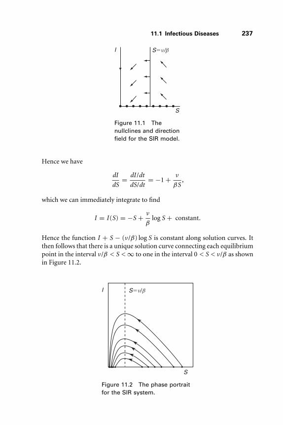
11.1 Infectious Diseases 237
S
S�m/bI
Figure 11.1 Thenullclines and directionfield for the SIR model.
Hence we have
dI
dS= dI /dt
dS/dt= −1 + ν
βS,
which we can immediately integrate to find
I = I (S) = −S + ν
βlog S + constant.
Hence the function I + S − (ν/β) log S is constant along solution curves. Itthen follows that there is a unique solution curve connecting each equilibriumpoint in the interval ν/β < S < ∞ to one in the interval 0 < S < ν/β as shownin Figure 11.2.
I S�m/b
S
Figure 11.2 The phase portraitfor the SIR system.

238 Chapter 11 Applications in Biology
A slightly more complicated model for infectious diseases arises when weassume that recovered individuals may lose their immunity and become rein-fected with the disease. Examples of this type of disease include malaria andtuberculosis. We assume that the return of recovered individuals to the class Soccurs at a rate proportional to the population of recovered individuals. Thisleads to the SIRS model (where the extra S indicates that recovered individualsmay reenter the susceptible group). The system becomes
S′ = −βSI + μR
I ′ = βSI − νI
R′ = νI − μR.
Again we see that the total population S + I + R is a constant, which wedenote by τ . We may eliminate R from this system by setting R = τ − S − I :
S′ = −βSI + μ(τ − S − I )
I ′ = βSI − νI .
Here β, μ, ν, and τ are all positive parameters.Unlike the SIR model, we now have at most two equilibria, one at (τ , 0) and
the other at
(S∗, I∗) =(
ν
β,μ(τ − ν
β)
ν + μ
).
The first equilibrium point corresponds to no disease whatsoever in the pop-ulation. The second equilibrium point only exists when τ ≥ ν/β. Whenτ = ν/β, we have a bifurcation as the two equilibria coalesce at (τ , 0). Thequantity ν/β is called the threshold level for the disease.
The linearized system is given by
Y ′ =(−βI − μ −βS − μ
βI βS − ν
)Y .
At the equilibrium point (τ , 0), the eigenvalues are −μ and βτ − ν, so thisequilibrium point is a saddle provided that the total population exceeds thethreshold level. At the second equilibrium point, a straightforward computa-tion shows that the trace of the matrix is negative, while the determinant ispositive. It then follows from the results in Chapter 4 that both eigenvalueshave negative real parts, and so this equilibrium point is asymptotically stable.

11.2 Predator/Prey Systems 239
Biologically, this means that the disease may become established in the com-munity only when the total population exceeds the threshold level. We willonly consider this case in what follows.
Note that the SIRS system is only of interest in the region given by I , S ≥ 0and S + I ≤ τ . Denote this triangular region by � (of course!). Note that theI -axis is no longer invariant, while on the S-axis, solutions increase up to theequilibrium at (τ , 0).
Proposition. The region � is positively invariant.
Proof: We check the direction of the vector field along the boundary of �.The field is tangent to the boundary along the lower edge I = 0 as well as at(0, τ ). Along S = 0 we have S′ = μ(τ − I ) > 0, so the vector field pointsinward for 0 < I < τ . Along the hypoteneuse, if 0 < S ≤ ν/β, we haveS′ = −βSI < 0 and I ′ = I (βS − ν) ≤ 0 so the vector field points inward.When ν/β < S < τ we have
−1 <I ′
S′ = −1 + ν
βS≤ 0
so again the vector field points inward. This completes the proof. �
The I -nullclines are given as in the SIR model by I = 0 and S = ν/β. TheS-nullcline is given by the graph of the function
I = I (S) = μ(τ − S)
βS + μ.
A calculus student will compute that I ′(S) < 0 and I ′′(S) > 0 when 0 ≤ S < τ .So this nullcline is the graph of a decreasing and concave up function that passesthrough both (τ , 0) and (0, τ ), as displayed in Figure 11.3. Note that in thisphase portrait, all solutions appear to tend to the equilibrium point (S∗, I∗);the proportion of infected to susceptible individuals tends to a “steady state.”To prove this, however, one would need to eliminate the possibility of closedorbits encircling the equilibrium point for a given set of parameters β, μ, ν,and τ .
11.2 Predator/Prey Systems
We next consider a pair of species, one of which consists of predators whosepopulation is denoted by y and the other its prey with population x . We assumethat the prey population is the total food supply for the predators. We also

240 Chapter 11 Applications in Biology
I
S�I�r
S
Figure 11.3 The nullclines andphase portrait in � for the SIRSsystem. Here β = ν = μ = 1 andτ = 2.
assume that, in the absence of predators, the prey population grows at a rateproportional to the current population. That is, as in Chapter 1, when y = 0we have x ′ = ax where a > 0. So in this case x(t ) = x0 exp(at ). Whenpredators are present, we assume that the prey population decreases at a rateproportional to the number of predator/prey encounters. As in the previoussection, one simple model for this is bxy where b > 0. So the differentialequation for the prey population is x ′ = ax − bxy .
For the predator population, we make more or less the opposite assump-tions. In the absence of prey, the predator population declines at a rateproportional to the current population. So when x = 0 we have y ′ = −cy withc > 0, and thus y(t ) = y0 exp(−ct ). The predator species becomes extinct inthis case. When there are prey in the environment, we assume that the predatorpopulation increases at a rate proportional to the predator/prey meetings, ordxy . We do not at this stage assume anything about overcrowding. Thus oursimplified predator/prey system (also called the Volterra-Lotka system) is
x ′ = ax − bxy = x(a − by)
y ′ = −cy + dxy = y(−c + dx)
where the parameters a, b, c , and d are all assumed to be positive. Since we aredealing with populations, we only consider x , y ≥ 0.
As usual, our first job is to locate the equilibrium points. These occur at theorigin and at (x , y) = (c/d , a/b). The linearized system is
X ′ =(
a − by −bxdy −c + dx
)X ,

11.2 Predator/Prey Systems 241
x
y
y�a/b
x�c/d
Figure 11.4 The nullclinesand direction field for thepredator/prey system.
so when x = y = 0 we have a saddle with eigenvalues a and −c . We know thestable and unstable curves: They are the y- and x-axes, respectively.
At the other equilibrium point (c/d , a/b), the eigenvalues are pure imaginary±i
√ac , and so we cannot conclude anything at this stage about stability of
this equilibrium point.We next sketch the nullclines for this system. The x-nullclines are given by
the straight lines x = 0 and y = a/b, whereas the y-nullclines are y = 0 andx = c/d . The nonzero nullcline lines separate the region x , y > 0 into four basicregions in which the vector field points as indicated in Figure 11.4. Hence thesolutions wind in the counterclockwise direction about the equilibrium point.
From this, we cannot determine the precise behavior of solutions: Theycould possibly spiral in toward the equilibrium point, spiral toward a limitcycle, spiral out toward “infinity” and the coordinate axes, or else lie on closedorbits. To make this determination, we search for a Liapunov function L.Employing the trick of separation of variables, we look for a function of theform
L(x , y) = F(x) + G(y).
Recall that L denotes the time derivative of L along solutions. We compute
L(x , y) = d
dtL(x(t ), y(t ))
= dF
dxx ′ + dG
dyy ′.
Hence
L(x , y) = xdF
dx(a − by) + y
dG
dy(−c + dx).

242 Chapter 11 Applications in Biology
We obtain L ≡ 0 provided
x dF /dx
dx − c≡ y dG/dy
by − a.
Since x and y are independent variables, this is possible if and only if
x dF /dx
dx − c= y dG/dy
by − a= constant.
Setting the constant equal to 1, we obtain
dF
dx= d − c
x,
dG
dy= b − a
y.
Integrating, we find
F(x) = dx − c log x ,
G(y) = by − a log y .
Thus the function
L(x , y) = dx − c log x + by − a log y
is constant on solution curves of the system when x , y > 0.By considering the signs of ∂L/∂x and ∂L/∂y it is easy to see that the equilib-
rium point Z = (c/d , a/b) is an absolute minimum for L. It follows that L [or,more precisely, L − L(Z )] is a Liapunov function for the system. Therefore Zis a stable equilibrium.
We note next that there are no limit cycles; this follows from Corollary 6in Section 10.6 because L is not constant on any open set. We now prove thefollowing theorem.
Theorem. Every solution of the predator/prey system is a closed orbit (exceptthe equilibrium point Z and the coordinate axes).
Proof: Consider the solution through W �= Z , where W does not lie on thex- or y-axis. This solution spirals around Z , crossing each nullcline infinitelyoften. Thus there is a doubly infinite sequence · · · < t−1 < t0 < t1 < · · ·such that φtn (W ) is on the line x = c/d , and tn → ±∞ as n → ±∞. IfW is not on a closed orbit, the points φtn (W ) are monotone along the line

11.2 Predator/Prey Systems 243
x�c/d
Figure 11.5 The nullclines andphase portrait for thepredator/prey system.
x = c/d , as discussed in the previous chapter. Since there are no limit cycles,either φtn (W ) → Z as n → ∞ or φtn (W ) → Z as n → −∞. Since L isconstant along the solution through W , this implies that L(W ) = L(Z ). Butthis contradicts minimality of L(Z ). This completes the proof. �
The phase portrait for this predator/prey system is displayed in Figure 11.5.We conclude that, for any given initial populations (x(0), y(0)) with x(0) �= 0and y(0) �= 0, other than Z , the populations of predator and prey oscillatecyclically. No matter what the populations of prey and predator are, neitherspecies will die out, nor will its population grow indefinitely.
Now let us introduce overcrowding into the prey equation. As in the logisticmodel in Chapter 1, the equations for prey, in the absence of predators, maybe written in the form
x ′ = ax − λx2.
We also assume that the predator population obeys a similar equation
y ′ = −cy − μy2
when x = 0. Incorporating the assumptions above yields the predator/preyequations for species with limited growth:
x ′ = x(a − by − λx)
y ′ = y(−c + dx − μy).

244 Chapter 11 Applications in Biology
As before, the parameters a, b, c , d as well as λ and μ are all positive. Wheny = 0, we have the logistic equation x ′ = x(a − λx), which yields equilibriaat the origin and at (a/λ, 0). As we saw in Chapter 1, all nonzero solutions onthe x-axis tend to a/λ.
When x = 0, the equation for y is y ′ = −cy −μy2. Since y ′ < 0 when y > 0,it follows that all solutions on this axis tend to the origin. Thus we confineattention to the upper-right quadrant Q where x , y > 0.
The nullclines are given by the x- and y-axes, together with the lines
L : a − by − λx = 0
M : −c + dx − μy = 0.
Along the lines L and M , we have x ′ = 0 and y ′ = 0, respectively. There aretwo possibilities, according to whether these lines intersect in Q or not.
We first consider the case where the two lines do not meet in Q. In this casewe have the nullcline configuration depicted in Figure 11.6. All solutions to theright of M head upward and to the left until they meet M ; between the lines Land M solutions now head downward and to the left. Thus they either meet Lor tend directly to the equilibrium point at (a/λ, 0). If solutions cross L, theythen head right and downward, but they cannot cross L again. Thus they tootend to (a/λ, 0). Thus all solutions in Q tend to this equilibrium point. Weconclude that, in this case, the predator population becomes extinct and theprey population approaches its limiting value of a/λ.
We may interpret the behavior of solutions near the nullclines as follows.Since both x ′ and y ′ are never both positive, it is impossible for both prey
ML
Figure 11.6 The nullclinesand phase portrait for apredator/prey system withlimited growth when thenullclines do not meet in Q.

11.2 Predator/Prey Systems 245
and predators to increase at the same time. If the prey population is aboveits limiting value, it must decrease. After a while the lack of prey causes thepredator population to begin to decrease (when the solution crosses M ). Afterthat point the prey population can never increase past a/λ, and so the predatorpopulation continues to decrease. If the solution crosses L, the prey populationincreases again (but not past a/λ), while the predators continue to die off. Inthe limit the predators disappear and the prey population stabilizes at a/λ.
Suppose now that L and M cross at a point Z = (x0, y0) in the quadrant Q;of course, Z is an equilibrium. The linearization of the vector field at Z is
X ′ =(−λx0 −bx0
dy0 −μy0
)X .
The characteristic polynomial has trace given by −λx0 − μy0 < 0 and deter-minant (bd + λμ)x0y0 > 0. From the trace-determinant plane of Chapter 4,we see that Z has eigenvalues that are either both negative or both complexwith negative real parts. Hence Z is asymptotically stable.
Note that, in addition to the equilibria at Z and (0, 0), there is still anequilibrium at (a/λ, 0). Linearization shows that this equilibrium is a saddle;its stable curve lies on the x-axis. See Figure 11.7.
It is not easy to determine the basin of Z , nor do we know whether thereare any limit cycles. Nevertheless we can obtain some information. The lineL meets the x-axis at (a/λ, 0) and the y-axis at (0, a/b). Let � be a rectanglewhose corners are (0, 0), (p, 0), (0, q), and (p, q) with p > a/λ, q > a/b, andthe point (p, q) lying in M . Every solution at a boundary point of � either
q
L
ΓM
p
Figure 11.7 The nullclines andphase portrait for a predator/preysystem with limited growth whenthe nullclines do meet in Q.

246 Chapter 11 Applications in Biology
enters � or is part of the boundary. Therefore � is positively invariant. Everypoint in Q is contained in such a rectangle.
By the Poincaré-Bendixson theorem, the ω-limit set of any point (x , y) in �,with x , y > 0, must be a limit cycle or contain one of the three equilibria (0, 0),Z , or (a/λ, 0). We rule out (0, 0) and (a/λ, 0) by noting that these equilibria aresaddles whose stable curves lie on the x- or y-axes. Therefore ω(x , y) is eitherZ or a limit cycle in �. By Corollary 4 of the Poincaré-Bendixson theorem anylimit cycle must surround Z .
We observe further that any such rectangle � contains all limit cycles,because a limit cycle (like any solution) must enter�, and � is positively invari-ant. Fixing (p, q) as above, it follows that for any initial values (x(0), y(0)),there exists t0 > 0 such that x(t ) < p, y(t ) < q if t ≥ t0. We conclude thatin the long run, a solution either approaches Z or else spirals down to a limitcycle.
From a practical standpoint a solution that tends toward Z is indistinguish-able from Z after a certain time. Likewise, a solution that approaches a limitcycle γ can be identified with γ after it is sufficiently close. We conclude thatany population of predators and prey that obeys these equations eventuallysettles down to either a constant or periodic population. Furthermore, thereare absolute upper bounds that no population can exceed in the long run, nomatter what the initial populations are.
11.3 Competitive Species
We consider now two species that compete for a common food supply. Insteadof analyzing specific equations, we follow a different procedure: We consider alarge class of equations about which we assume only a few qualitative features.In this way considerable generality is gained, and little is lost because specificequations can be very difficult to analyze.
Let x and y denote the populations of the two species. The equations ofgrowth of the two populations may be written in the form
x ′ = M (x , y)x
y ′ = N (x , y)y
where the growth rates M and N are functions of both variables. As usual, weassume that x and y are nonnegative. So the x-nullclines are given by x = 0and M (x , y) = 0 and the y-nullclines are y = 0 and N (x , y) = 0. We makethe following assumptions on M and N :
1. Because the species compete for the same resources, if the populationof either species increases, then the growth rate of the other goes down.
11.3 Competitive Species 247
Hence
∂M
∂y< 0 and
∂N
∂x< 0.
2. If either population is very large, both populations decrease. Hence thereexists K > 0 such that
M (x , y) < 0 and N (x , y) < 0 if x ≥ K or y ≥ K .
3. In the absence of either species, the other has a positive growth rate upto a certain population and a negative growth rate beyond it. Thereforethere are constants a, b > 0 such that
M (x , 0) > 0 for x < a and M (x , 0) < 0 for x > a,
N (0, y) > 0 for y < b and N (0, y) < 0 for y > b.
By conditions (1) and (3) each vertical line {x} × R meets the set μ =M−1(0) exactly once if 0 ≤ x ≤ a and not at all if x > a. By condition (1)and the implicit function theorem, μ is the graph of a nonnegative functionf : [0, a] → R such that f −1(0) = a. Below the curve μ, M is positive andabove it, M is negative. In the same way the set ν = N −1(0) is a smooth curveof the form
{(x , y) | x = g (y)
},
where g : [0, b] → R is a nonnegative function with g−1(0) = b. The functionN is positive to the left of ν and negative to the right.
Suppose first that μ and ν do not intersect and that μ is below ν. Thenthe phase portrait can be determined immediately from the nullclines. Theequilibria are (0, 0), (a, 0), and (0, b). The origin is a source, while (a, 0) is asaddle (assuming that (∂M /∂x)(a, 0) < 0). The equilibrium at (0, b) is a sink[again assuming that (∂N /∂y)(0, b) < 0]. All solutions with y0 > 0 tend tothe asymptotically stable equilibrium (0, b) with the exception of solutions onthe x-axis. See Figure 11.8. In the case where μ lies above ν, the situation isreversed, and all solutions with x0 > 0 tend to the sink that now appears at(a, 0).
Suppose now that μ and ν intersect. We make the assumption that μ ∩ ν
is a finite set, and at each intersection point, μ and ν cross transversely, thatis, they have distinct tangent lines at the intersection points. This assumptionmay be eliminated; we make it only to simplify the process of determining theflow.

248 Chapter 11 Applications in Biology
a
b m
l
Figure 11.8 The phase portraitwhen μ and ν do not meet.
The nullclines μ and ν and the coordinate axes bound a finite number ofconnected open sets in the upper-right quadrant: These are the basic regionswhere x ′ �= 0 and y ′ �= 0. They are of four types:
A : x ′ > 0, y ′ > 0, B : x ′ < 0, y ′ > 0;
C : x ′ < 0, y ′ < 0, D : x ′ > 0, y ′ < 0.
Equivalently, these are the regions where the vector field points northeast,northwest, southwest, or southeast, respectively. Some of these regions areindicated in Figure 11.9. The boundary ∂R of a basic region R is made up ofpoints of the following types: points of μ ∩ ν, called vertices; points on μ or ν
but not on both nor on the coordinate axes, called ordinary boundary points;and points on the axes.
A vertex is an equilibrium; the other equilibria lie on the axes at (0, 0), (a, 0),and (0, b). At an ordinary boundary point Z ∈ ∂R, the vector field is eithervertical (if Z ∈ μ) or horizontal (if Z ∈ ν). This vector points either into or outof R since μ has no vertical tangents and ν has no horizontal tangents. We callZ an inward or outward point of ∂R, accordingly. Note that, in Figure 11.9,the vector field either points inward at all ordinary points on the boundary ofa basic region, or else it points outward at all such points. This is no accident,for we have:
Proposition. Let R be a basic region for the competitive species model. Thenthe ordinary boundary points of R are either all inward or all outward.
Proof: There are only two ways in which the curves μ and ν can intersect ata vertex P . As y increases along ν, the curve ν may either pass from below μ

11.3 Competitive Species 249
lm
C
D
S
R
B
Qb
P
a
A
Figure 11.9 The basic regionswhen the nullclines μ and ν
intersect.
to above μ, or from above to below μ. These two scenarios are illustrated inFigures 11.10a and b. There are no other possibilities since we have assumedthat these curves cross transversely.
Since x ′ > 0 below μ and x ′ < 0 above μ, and since y ′ > 0 to the left of ν
and y ′ < 0 to the right, we therefore have the following configurations for thevector field in these two cases. See Figure 11.11.
In each case we see that the vector field points inward in two opposite basicregions abutting P , and outward in the other two basic regions.
If we now move along μ or ν to the next vertex along this curve, we see thatadjacent basic regions must maintain their inward or outward configuration.Therefore, at all ordinary boundary points on each basic region, the vectorfield either points outward or points inward, as required. �
l l
m
m
(a) (b)
Figure 11.10 In (a), ν passes from below μ to above μ as y
increases. The situation is reversed in (b).

250 Chapter 11 Applications in Biology
ll
m
m
Figure 11.11 Configurations of the vector field nearvertices.
As a consequence of the proposition, it follows that each basic region andits closure is either positively or negatively invariant. What are the possibleω-limit points of this system? There are no closed orbits. A closed orbit mustbe contained in a basic region, but this is impossible since x(t ) and y(t ) aremonotone along any solution curve in a basic region. Therefore all ω-limitpoints are equilibria.
We note also that each solution is defined for all t ≥ 0, because any pointlies in a large rectangle � with corners at (0, 0), (x0, 0), (0, y0), and (x0, y0) withx0 > a and y0 > b; such a rectangle is positively invariant. See Figure 11.12.Thus we have shown:
Theorem. The flow φt of the competitive species system has the followingproperty: For all points (x , y), with x ≥ 0, y ≥ 0, the limit
limt→∞ φt (x , y)
exists and is one of a finite number of equilibria. �
lΓ
m
Figure 11.12 All solutions must enterand then remain in �.

11.3 Competitive Species 251
l
m P
Figure 11.13 This configuration of μ and ν
leads to an asymptotically stable equilibriumpoint.
We conclude that the populations of two competing species always tend toone of a finite number of limiting populations.
Examining the equilibria for stability, one finds the following results. A ver-tex where μ and ν each have negative slope, but μ is steeper, is asymptoticallystable. See Figure 11.13. One sees this by drawing a small rectangle with sidesparallel to the axes around the equilibrium, putting one corner in each of thefour adjacent basic regions. Such a rectangle is positively invariant; since it canbe arbitrarily small, the equilibrium is asymptotically stable.
This may also be seen as follows. We have
slope of μ = −Mx
My< slope of ν = −Nx
Ny< 0,
where Mx = ∂M /∂x , My = ∂M /∂y , and so on, at the equilibrium. Now recallthat My < 0 and Nx < 0. Therefore, at the equilibrium point, we also haveMx < 0 and Ny < 0. Linearization at the equilibrium point yields the matrix(
xMx xMy
yNx yNy
).
The trace of this matrix is xMx +yMy < 0 while the determinant is xy(MxNy −MyNx) > 0. Thus the eigenvalues have negative real parts, and so we have asink.
A case-by-case study of the different ways μ and ν can cross shows that theonly other asymptotically stable equilibrium in this model is (0, b) when (0, b)is above μ, or (a, 0) when (a, 0) is to the right of ν. All other equilibria areunstable. There must be at least one asymptotically stable equilibrium. If (0, b)is not one, then it lies under μ; and if (a, 0) is not one, it lies over μ. In thatcase μ and ν cross, and the first crossing to the left of (a, 0) is asymptoticallystable.

252 Chapter 11 Applications in Biology
l
Z
R
P
S
Q
b
B∞
B∞
m
Figure 11.14 Note that solutions on either side ofthe point Z in the stable curve of Q have verydifferent fates.
For example, this analysis tells us that, in Figure 11.14, only P and (0, b) areasymptotically stable; all other equilibria are unstable. In particular, assumingthat the equilibrium Q in Figure 11.14 is hyperbolic, then it must be a saddlebecause certain nearby solutions tend toward it, while others tend away. Thepoint Z lies on one branch of the stable curve through Q. All points in theregion denoted B∞ to the left of Z tend to the equilibrium at (0, b), whilepoints to the right go to P . Thus as we move across the branch of the stablecurve containing Z , the limiting behavior of solutions changes radically. Sincesolutions just to the right of Z tend to the equilibrium point P , it follows thatthe populations in this case tend to stabilize. On the other hand, just to theleft of Z , solutions tend to an equilibrium point where x = 0. Thus in thiscase, one of the species becomes extinct. A small change in initial conditionshas led to a dramatic change in the fate of populations. Ecologically, this smallchange could have been caused by the introduction of a new pesticide, theimportation of additional members of one of the species, a forest fire, or thelike. Mathematically, this event is a jump from the basin of P to that of (0, b).
11.4 Exploration: Competition and
Harvesting
In this exploration we will investigate the competitive species model where weallow either harvesting (emigration) or immigration of one of the species. We

Exercises 253
consider the system
x ′ = x(1 − ax − y)
y ′ = y(b − x − y) + h.
Here a, b, and h are parameters. We assume that a, b > 0. If h < 0, then we areharvesting species y at a constant rate, whereas if h > 0, we add to the popula-tion y at a constant rate. The goal is to understand this system completely forall possible values of these parameters. As usual, we only consider the regimewhere x , y ≥ 0. If y(t ) < 0 for any t > 0, then we consider this species to havebecome extinct.
1. First assume that h = 0. Give a complete synopsis of the behavior of thissystem by plotting the different behaviors you find in the a, b parameterplane.
2. Identify the points or curves in the ab–plane where bifurcations occurwhen h = 0 and describe them.
3. Now let h < 0. Describe the ab–parameter plane for various (fixed)h-values.
4. Repeat the previous exploration for h > 0.5. Describe the full three-dimensional parameter space using pictures, flip
books, 3D models, movies, or whatever you find most appropriate.
E X E R C I S E S
1. For the SIRS model, prove that all solutions in the triangular region �
tend to the equilibrium point (τ , 0) when the total population does notexceed the threshold level for the disease.
2. Sketch the phase plane for the following variant of the predator/preysystem:
x ′ = x(1 − x) − xy
y ′ = y(1 − y
x
).
3. A modification of the predator/prey equations is given by
x ′ = x(1 − x) − axy
x + 1
y ′ = y(1 − y)
where a > 0 is a parameter.

254 Chapter 11 Applications in Biology
(a) Find all equilibrium points and classify them.
(b) Sketch the nullclines and the phase portraits for different values of a.
(c) Describe any bifurcations that occur as a varies.
4. Another modification of the predator/prey equations is given by
x ′ = x(1 − x) − xy
x + b
y ′ = y(1 − y)
where b > 0 is a parameter.
(a) Find all equilibrium points and classify them.
(b) Sketch the nullclines and the phase portraits for different valuesof b.
(c) Describe any bifurcations that occur as b varies.
5. The equations
x ′ = x(2 − x − y),
y ′ = y(3 − 2x − y)
satisfy conditions (1) through (3) in Section 11.3 for competing species.Determine the phase portrait for this system. Explain why these equationsmake it mathematically possible, but extremely unlikely, for both speciesto survive.
6. Consider the competing species model
x ′ = x(a − x − ay)
y ′ = y(b − bx − y)
where the parameters a and b are positive.
(a) Find all equilibrium points for this system and determine theirstability type. These types will, of course, depend on a and b.
(b) Use the nullclines to determine the various phase portraits that arisefor different choices of a and b.
(c) Determine the values of a and b for which there is a bifurcation inthis system and describe the bifurcation that occurs.
(d) Record your findings by drawing a picture of the ab–plane andindicating in each open region of this plane the qualitative structureof the corresponding phase portraits.

Exercises 255
7. Two species x , y are in symbiosis if an increase of either population leadsto an increase in the growth rate of the other. Thus we assume
x ′ = M (x , y)x
y ′ = N (x , y)y
with
∂M
∂y> 0 and
∂N
∂x> 0
and x , y ≥ 0. We also suppose that the total food supply is limited; hencefor some A > 0, B > 0 we have
M (x , y) < 0 if x > A,
N (x , y) < 0 if y > B.
If both populations are very small, they both increase; hence
M (0, 0) > 0 and N (0, 0) > 0.
Assuming that the intersections of the curves M−1(0), N −1(0) are finite,and that all are transverse, show the following:
(a) Every solution tends to an equilibrium in the region 0 < x < A,0 < y < B.
(b) There are no sources.(c) There is at least one sink.(d) If ∂M /∂x < 0 and ∂N /∂y < 0, there is a unique sink Z , and Z is the
ω-limit set for all (x , y) with x > 0, y > 0.
8. Give a system of differential equations for a pair of mutually destruc-tive species. Then prove that, under plausible hypotheses, two mutuallydestructive species cannot coexist in the long run.
9. Let y and x denote predator and prey populations. Let
x ′ = M (x , y)x
y ′ = N (x , y)y
where M and N satisfy the following conditions.
(a) If there are not enough prey, the predators decrease. Hence for someb > 0
N (x , y) < 0 if x < b.

256 Chapter 11 Applications in Biology
(b) An increase in the prey improves the predator growth rate; hence∂N /∂x > 0.
(c) In the absence of predators a small prey population will increase;hence M (0, 0) > 0.
(d) Beyond a certain size, the prey population must decrease; hencethere exists A > 0 with M (x , y) < 0 if x > A.
(e) Any increase in predators decreases the rate of growth of prey; hence∂M /∂y < 0.
(f) The two curves M−1(0), N −1(0) intersect transversely and at only afinite number of points.
Show that if there is some (u, v) with M (u, v) > 0 and N (u, v) > 0 thenthere is either an asymptotically stable equilibrium or an ω-limit cycle.Moreover, show that, if the number of limit cycles is finite and positive,one of them must have orbits spiraling toward it from both sides.
10. Consider the following modification of the predator/prey equations:
x ′ = x(1 − x) − axy
x + c
y ′ = by(1 − y
x
)where a, b, and c are positive constants. Determine the region in theparameter space for which this system has a stable equilibrium with bothx , y �= 0. Prove that, if the equilibrium point is unstable, this system hasa stable limit cycle.

12Applications in
Circuit Theory
In this chapter we first present a simple but very basic example of an electricalcircuit and then derive the differential equations governing this circuit. Certainspecial cases of these equations are analyzed using the techniques developedin Chapters 8 through 10 in the next two sections; these are the classicalequations of Lienard and van der Pol. In particular, the van der Pol equationcould perhaps be regarded as one of the fundamental examples of a nonlinearordinary differential equation. It possesses an oscillation or periodic solutionthat is a periodic attractor. Every nontrivial solution tends to this periodicsolution; no linear system has this property. Whereas asymptotically stableequilibria sometimes imply death in a system, attracting oscillators imply life.We give an example in Section 12.4 of a continuous transition from one suchsituation to the other.
12.1 An RLC Circuit
In this section, we present our first example of an electrical circuit. This circuitis the simple but fundamental series RLC circuit displayed in Figure 12.1. Webegin by explaining what this diagram means in mathematical terms. Thecircuit has three branches, one resistor marked by R, one inductor marked byL, and one capacitor marked by C . We think of a branch of this circuit as a
257
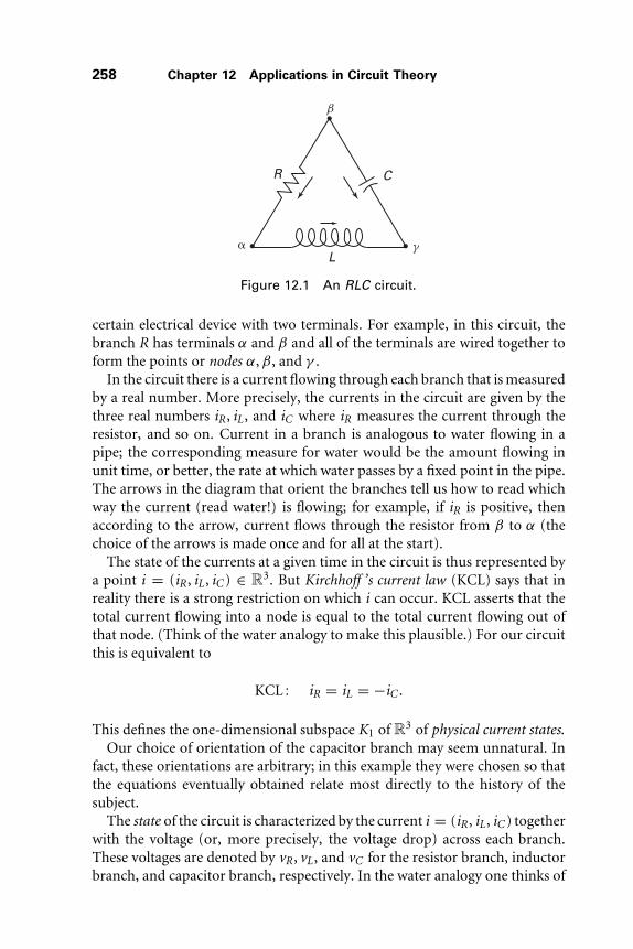
258 Chapter 12 Applications in Circuit Theory
R
L
C
� c
b
Figure 12.1 An RLC circuit.
certain electrical device with two terminals. For example, in this circuit, thebranch R has terminals α and β and all of the terminals are wired together toform the points or nodes α, β, and γ .
In the circuit there is a current flowing through each branch that is measuredby a real number. More precisely, the currents in the circuit are given by thethree real numbers iR , iL , and iC where iR measures the current through theresistor, and so on. Current in a branch is analogous to water flowing in apipe; the corresponding measure for water would be the amount flowing inunit time, or better, the rate at which water passes by a fixed point in the pipe.The arrows in the diagram that orient the branches tell us how to read whichway the current (read water!) is flowing; for example, if iR is positive, thenaccording to the arrow, current flows through the resistor from β to α (thechoice of the arrows is made once and for all at the start).
The state of the currents at a given time in the circuit is thus represented bya point i = (iR , iL , iC ) ∈ R3. But Kirchhoff ’s current law (KCL) says that inreality there is a strong restriction on which i can occur. KCL asserts that thetotal current flowing into a node is equal to the total current flowing out ofthat node. (Think of the water analogy to make this plausible.) For our circuitthis is equivalent to
KCL : iR = iL = −iC .
This defines the one-dimensional subspace K1 of R3 of physical current states.Our choice of orientation of the capacitor branch may seem unnatural. In
fact, these orientations are arbitrary; in this example they were chosen so thatthe equations eventually obtained relate most directly to the history of thesubject.
The state of the circuit is characterized by the current i = (iR , iL , iC ) togetherwith the voltage (or, more precisely, the voltage drop) across each branch.These voltages are denoted by vR , vL , and vC for the resistor branch, inductorbranch, and capacitor branch, respectively. In the water analogy one thinks of

12.1 An RLC Circuit 259
the voltage drop as the difference in pressures at the two ends of a pipe. Tomeasure voltage, one places a voltmeter (imagine a water pressure meter) ateach of the nodes α, β, and γ that reads V (α) at α, and so on. Then vR is thedifference in the reading at α and β
V (β) − V (α) = vR .
The direction of the arrow tells us that vR = V (β)−V (α) rather than V (α)−V (β).
An unrestricted voltage state of the circuit is then a point v = (vR , vL , vC ) ∈R3. This time the Kirchhoff voltage law puts a physical restriction on v :
KVL : vR + vL − vC = 0.
This defines a two-dimensional subspace K2 of R3. KVL follows immediatelyfrom our definition of the vR , vL , and vC in terms of voltmeters; that is,
vR + vL − vC = (V (β) − V (α)) + (V (α) − V (γ )) − (V (β) − V (γ )) = 0.
The product space R3 × R3 is called the state space for the circuit. Thosestates (i, v) ∈ R3 × R3 satisfying Kirchhoff’s laws form a three-dimensionalsubspace of the state space.
Now we give a mathematical definition of the three kinds of electrical devicesin the circuit. First consider the resistor element. A resistor in the R branchimposes a “functional relationship” on iR and vR . We take in our examplethis relationship to be defined by a function f : R → R, so that vR = f (iR).If R is a conventional linear resistor, then f is linear and so f (iR) = kiR .This relation is known as Ohm’s law. Nonlinear functions yield a generalizedOhm’s law. The graph of f is called the characteristic of the resistor. A coupleof examples of characteristics are given in Figure 12.2. (A characteristic likethat in Figure 12.2b occurs in a “tunnel diode.”)
A physical state (i, v) ∈ R3 × R3 is a point that satisfies KCL, KVL, and alsof (iR) = vR . These conditions define the set of physical states � ⊂ R3 × R3.Thus � is the set of points (iR , iL , iC , vR , vL , vC ) in R3 × R3 that satisfy:
1. iR = iL = −iC (KCL);2. vR + vL − vC = 0 (KVL);3. f (iR) = vR (generalized Ohm’s law).
Now we turn to the differential equations governing the circuit. The induc-tor (which we think of as a coil; it is hard to find a water analogy) specifiesthat
LdiL(t )
dt= vL(t ) (Faraday’s law),

260 Chapter 12 Applications in Circuit Theory
(a) (b)
VR
iR
VR
iR
Figure 12.2 Several possible characteristics for aresistor.
where L is a positive constant called the inductance. On the other hand, thecapacitor (which may be thought of as two metal plates separated by someinsulator; in the water model it is a tank) imposes the condition
CdvC (t )
dt= iC (t )
where C is a positive constant called the capacitance.Let’s summarize the development so far: a state of the circuit is given by the
six numbers (iR , iL , iC , vR , vL , vC ), that is, a point in the state space R3 × R3.These numbers are subject to three restrictions: Kirchhoff’s current law,Kirchhoff’s voltage law, and the resistor characteristic or generalized Ohm’slaw. Therefore the set of physical states is a certain subset � ⊂ R3 × R3.The way a state changes in time is determined by the two previous differentialequations.
Next, we simplify the set of physical states � by observing that iL and vC
determine the other four coordinates. This follows since iR = iL and iC = −iLby KCL, vR = f (iR) = f (iL) by the generalized Ohm’s law, and vL = vC −vR =vC −f (iL) by KVL. Therefore we can use R2 as the state space, with coordinatesgiven by (iL , vC ). Formally, we define a map π : R3 × R3 → R2, which sends(i, v) ∈ R3 × R3 to (iL , vC ). Then we set π0 = π | �, the restriction of π to�. The map π0 : � → R2 is one to one and onto; its inverse is given by themap ψ : R2 → �, where
ψ(iL , vC ) = (iL , iL , −iL , f (iL), vC − f (iL), vC ).
It is easy to check that ψ(iL , vC ) satisfies KCL, KVL, and the generalized Ohm’slaw, so ψ does map R2 into �. It is also easy to see that π0 and ψ are inverseto each other.
We therefore adopt R2 as our state space. The differential equationsgoverning the change of state must be rewritten in terms of our new

12.2 The Lienard Equation 261
coordinates (iL , vC ):
LdiLdt
= vL = vC − f (iL)
CdvC
dt= iC = −iL .
For simplicity, and since this is only an example, we set L = C = 1. If wewrite x = iL and y = vC , we then have a system of differential equations inthe plane of the form
dx
dt= y − f (x)
dy
dt= −x .
This is one form of the equation known as the Lienard equation. We analyzethis system in the following section.
12.2 The Lienard Equation
In this section we begin the study of the phase portrait of the Lienard systemfrom the circuit of the previous section, namely:
dx
dt= y − f (x)
dy
dt= −x .
In the special case where f (x) = x3 − x , this system is called the van der Polequation.
First consider the simplest case where f is linear. Suppose f (x) = kx , wherek > 0. Then the Lienard system takes the form Y ′ = AY where
A =(−k 1
−1 0
).
The eigenvalues of A are given by λ± = (−k ±(k2 −4)1/2)/2. Since λ± is eithernegative or else has a negative real part, the equilibrium point at the origin isa sink. It is a spiral sink if k < 2. For any k > 0, all solutions of the system tendto the origin; physically, this is the dissipative effect of the resistor.

262 Chapter 12 Applications in Circuit Theory
Note that we have
y ′′ = −x ′ = −y + kx = −y − ky ′,
so that the system is equivalent to the second-order equation y ′′ +ky ′ +y = 0,which is often encountered in elementary differential equations courses.
Next we consider the case of a general characteristic f . There is a unique equi-librium point for the Lienard system that is given by (0, f (0)). Linearizationyields the matrix (−f ′(0) 1
−1 0
)
whose eigenvalues are given by
λ± = 1
2
(−f ′(0) ±
√(f ′(0))2 − 4
).
We conclude that this equilibrium point is a sink if f ′(0) > 0 and a source iff ′(0) < 0. In particular, for the van der Pol equation where f (x) = x3 − x , theunique equilibrium point is a source.
To analyze the system further, we define the function W : R2 → R2 byW (x , y) = 1
2 (x2 + y2). Then we have
W = x(y − f (x)) + y(−x) = −xf (x).
In particular, if f satisfies f (x) > 0 if x > 0, f (x) < 0 if x < 0, and f (0) = 0,then W is a strict Liapunov function on all of R2. It follows that, in this case,all solutions tend to the unique equilibrium point lying at the origin.
In circuit theory, a resistor is called passive if its characteristic is containedin the set consisting of (0, 0) and the interior of the first and third quadrant.Therefore in the case of a passive resistor, −xf (x) is negative except whenx = 0, and so all solutions tend to the origin. Thus the word passive correctlydescribes the dynamics of such a circuit.
12.3 The van der Pol Equation
In this section we continue the study of the Lienard equation in the specialcase where f (x) = x3 − x . This is the van der Pol equation:
dx
dt= y − x3 + x

12.3 The van der Pol Equation 263
dy
dt= −x .
Let φt denote the flow of this system. In this case we can give a fairly completephase portrait analysis.
Theorem. There is one nontrivial periodic solution of the van der Pol equationand every other solution (except the equilibrium point at the origin) tends to thisperiodic solution. “The system oscillates.” �
We know from the previous section that this system has a unique equilib-rium point at the origin, and that this equilibrium is a source, since f ′(0) < 0.The next step is to show that every nonequilibrium solution “rotates” in acertain sense around the equilibrium in a clockwise direction. To see this, notethat the x-nullcline is given by y = x3 − x and the y-nullcline is the y-axis.We subdivide each of these nullclines into two pieces given by
v+ = { (x , y) | y > 0, x = 0}v− = { (x , y) | y < 0, x = 0}g+ = { (x , y) | x > 0, y = x3 − x}g− = { (x , y) | x < 0, y = x3 − x}.
These curves are disjoint; together with the origin they form the boundariesof the four basic regions A, B, C , and D depicted in Figure 12.3.
From the configuration of the vector field in the basic regions, it appearsthat all nonequilibrium solutions wind around the origin in the clockwisedirection. This is indeed the case.
Proposition. Solution curves starting on v+ cross successively through g+,v−, and g− before returning to v+.
D
C
B
A
g�
m�
m�
g�
Figure 12.3 The basic regions and nullclines for thevan der Pol system.

264 Chapter 12 Applications in Circuit Theory
Proof: Any solution starting on v+ immediately enters the region A sincex ′(0) > 0. In A we have y ′ < 0, so this solution must decrease in the y direction.Since the solution cannot tend to the source, it follows that this solution musteventually meet g+. On g+ we have x ′ = 0 and y ′ < 0. Consequently, thesolution crosses g+, then enters the region B. Once inside B, the solutionheads southwest. Note that the solution cannot reenter A since the vector fieldpoints straight downward on g+. There are thus two possibilities: Either thesolution crosses v−, or else the solution tends to −∞ in the y direction andnever crosses v−.
We claim that the latter cannot happen. Suppose that it does. Let (x0, y0)be a point on this solution in region B and consider φt (x0, y0) = (x(t ), y(t )).Since x(t ) is never 0, it follows that this solution curve lies for all time in thestrip S given by 0 < x ≤ x0, y ≤ y0, and we have y(t ) → −∞ as t → t0 forsome t0. We first observe that, in fact, t0 = ∞. To see this, note that
y(t ) − y0 =∫ t
0y ′(s) ds =
∫ t
0−x(s) ds.
But 0 < x(s) ≤ x0, so we may only have y(t ) → −∞ if t → ∞.Now consider x(t ) for 0 ≤ t < ∞. We have x ′ = y − x3 + x . Since the
quantity −x3 + x is bounded in the strip S and y(t ) → −∞ as t → ∞, itfollows that
x(t ) − x0 =∫ t
0x ′(s) ds → −∞
as t → ∞ as well. But this contradicts our assumption that x(t ) > 0.Hence this solution must cross v−. Now the vector field is skew-symmetric
about the origin. That is, if G(x , y) is the van der Pol vector field, thenG(−x , −y) = −G(x , y). Exploiting this symmetry, it follows that solutionsmust then pass through regions C and D in similar fashion. �
As a consequence of this result, we may define a Poincaré map P on thehalf-line v+. Given (0, y0) ∈ v+, we define P(y0) to be the y coordinate of thefirst return of φt (0, y0) to v+ with t > 0. See Figure 12.4. As in Section 10.3,P is a one to one C∞ function. The Poincaré map is also onto. To see this,simply follow solutions starting on v+ backward in time until they reintersectv+, as they must by the proposition. Let Pn = P ◦ Pn−1 denote the n-foldcomposition of P with itself.
Our goal now is to prove the following theorem:
Theorem. The Poincaré map has a unique fixed point in v+. Furthermore,the sequence Pn(y0) tends to this fixed point as n → ∞ for any nonzeroy0 ∈ v+. �

12.3 The van der Pol Equation 265
y
m�
m�
g�
g�
P (y)
Figure 12.4 The Poincaré mapon v+.
Clearly, any fixed point of P lies on a periodic solution. On the otherhand, if P(y0) �= y0, then the solution through (0, y0) can never be periodic.Indeed, if P(y0) > y0, then the successive intersection of φt (0, y0) with v+ isa monotone sequence as in Section 10.4. Hence the solution crosses v+ in anincreasing sequence of points and so the solution can never meet itself. Thecase P(y0) < y0 is analogous.
We may define a “semi-Poincaré map” α : v+ → v− by letting α(y) be they coordinate of the first point of intersection of φt (0, y) with v− where t > 0.Also define
δ(y) = 1
2
(α(y)2 − y2) .
Note for later use that there is a unique point (0, y∗) ∈ v+ and time t∗ suchthat
1. φt (0, y∗) ∈ A for 0 < t < t∗;2. φt∗(0, y∗) = (1, 0) ∈ g+.
See Figure 12.5.The theorem will now follow directly from the following rather delicate
result.
Proposition. The function δ(y) satisfies:
1. δ(y) > 0 if 0 < y < y∗;2. δ(y) decreases monotonically to −∞ as y → ∞ for y > y∗. �
We will prove the proposition shortly; first we use it to complete the proofof the theorem. We exploit the fact that the vector field is skew-symmetric

266 Chapter 12 Applications in Circuit Theory
m� g�
m�
(1, 0)
y*
y
a(y)
Figure 12.5 Thesemi-Poincaré map.
about the origin. This implies that if (x(t ), y(t )) is a solution curve, then so is(−x(t ), −y(t )).
Part of the graph of δ(y) is shown schematically in Figure 12.6. The interme-diate value theorem and the proposition imply that there is a unique y0 ∈ v+with δ(y0) = 0. Consequently, α(y0) = −y0 and it follows from the skew-symmetry that the solution through (0, y0) is periodic. Since δ(y) �= 0 exceptat y0, we have α(y) �= y for all other y-values, and so it follows that φt (0, y0)is the unique periodic solution.
We next show that all other solutions (except the equilibrium point) tendto this periodic solution. Toward that end, we define a map β : v− → v+,sending each point of v− to the first intersection of the solution (for t > 0)with v+. By symmetry we have
β(y) = −α(−y).
Note also that P(y) = β ◦ α(y).
y* y0y
d(y)
Figure 12.6 Thegraph of δ(y).

12.3 The van der Pol Equation 267
We identify the y-axis with the real numbers in the y coordinate. Thus ify1, y2 ∈ v+ ∪ v− we write y1 > y2 if y1 is above y2. Note that α and β reversethis ordering while P preserves it.
Now choose y ∈ v+ with y > y0. Since α(y0) = −y0 we have α(y) < −y0
and P(y) > y0. On the other hand, δ(y) < 0, which implies that α(y) > −y .Therefore P(y) = β(α(y)) < y . We have shown that y > y0 implies y > P(y) >y0. Similarly P(y) > P(P(y)) > y0 and by induction Pn(y) > Pn+1(y) > y0
for all n > 0.The decreasing sequence Pn(y) has a limit y1 ≥ y0 in v+. Note that y1 is a
fixed point of P , because, by continuity of P , we have
P(y1) − y1 = limn→∞ P(Pn(y)) − y1
= y1 − y1 = 0.
Since P has only one fixed point, we have y1 = y0. This shows that the solutionthrough y spirals toward the periodic solution as t → ∞. See Figure 12.7. Thesame is true if y < y0; the details are left to the reader. Since every solutionexcept the equilibrium meets v+, the proof of the theorem is complete. �
Finally, we turn to the proof of the proposition. We adopt the followingnotation. Let γ : [a, b] → R2 be a smooth curve in the plane and let F : R2 →R. We write γ (t ) = (x(t ), y(t )) and define
∫γ
F(x , y) =∫ b
aF(x(t ), y(t )) dt .
Figure 12.7 The phaseportrait of the van der Polequation.

268 Chapter 12 Applications in Circuit Theory
If it happens that x ′(t ) �= 0 for a ≤ t ≤ b, then along γ , y is a function of x ,so we may write y = y(x). In this case we can change variables:
∫ b
aF(x(t ), y(t )) dt =
∫ x(b)
x(a)F(x , y(x))
dt
dxdx .
Therefore ∫γ
F(x , y) =∫ x(b)
x(a)
F(x , y(x))
dx/dtdx .
We have a similar expression if y ′(t ) �= 0.Now recall the function
W (x , y) = 1
2
(x2 + y2)
introduced in the previous section. Let p ∈ v+. Suppose α(p) = φτ (p). Letγ (t ) = (x(t ), y(t )) for 0 ≤ t ≤ τ = τ (p) be the solution curve joining p ∈ v+to α(p) ∈ v−. By definition
δ(p) = 1
2
(y(τ )2 − y(0)2)
= W (x(τ ), y(τ )) − W (x(0), y(0)).
Thus
δ(p) =∫ τ
0
d
dtW (x(t ), y(t )) dt .
Recall from Section 12.2 that we have
W = −xf (x) = −x(x3 − x).
Thus we have
δ(p) =∫ τ
0−x(t )(x(t )3 − x(t )) dt
=∫ τ
0x(t )2(1 − x(t )2) dt .
This immediately proves part (1) of the proposition because the integrand ispositive for 0 < x(t ) < 1.

12.3 The van der Pol Equation 269
g�
y1
y2
y0
c3
c2
c1
Figure 12.8 The curves γ1 , γ2 ,and γ3 depicted on the closedorbit through y0 .
We may rewrite the last equality as
δ(p) =∫
γ
x2 (1 − x2) .
We restrict attention to points p ∈ v+ with p > y∗. We divide the correspond-ing solution curve γ into three curves γ1, γ2, γ3 as displayed in Figure 12.8.The curves γ1 and γ3 are defined for 0 ≤ x ≤ 1, while the curve γ2 is definedfor y1 ≤ y ≤ y2. Then
δ(p) = δ1(p) + δ2(p) + δ3(p)
where
δi(p) =∫
γi
x2 (1 − x2) , i = 1, 2, 3.
Notice that, along γ1, y(t ) may be regarded as a function of x . Hence we have
δ1(p) =∫ 1
0
x2(1 − x2
)dx/dt
dx
=∫ 1
0
x2(1 − x2
)y − f (x)
dx
where f (x) = x3 − x . As p moves up the y-axis, y − f (x) increases [for (x , y)on γ1]. Hence δ1(p) decreases as p increases. Similarly δ3(p) decreases as pincreases.

270 Chapter 12 Applications in Circuit Theory
On γ2, x(t ) may be regarded as a function of y , which is defined for y ∈[y1, y2] and x ≥ 1. Therefore since dy/dt = −x , we have
δ2(p) =∫ y1
y2
−x(y)(1 − x(y)2) dy
=∫ y2
y1
x(y)(1 − x(y)2) dy
so that δ2(p) is negative.As p increases, the domain [y1, y2] of integration becomes steadily larger.
The function y → x(y) depends on p, so we write it as xp(y). As pincreases, the curves γ2 move to the right; hence xp(y) increases and soxp(y)(1 − xp(y)2) decreases. It follows that δ2(p) decreases as p increases;and evidently limp→∞ δ2(p) = −∞. Consequently, δ(p) also decreases andtends to −∞ as p → ∞. This completes the proof of the proposition.
12.4 A Hopf Bifurcation
We now describe a more general class of circuit equations where the resistorcharacteristic depends on a parameter μ and is denoted by fμ. (Perhaps μ isthe temperature of the resistor.) The physical behavior of the circuit is thendescribed by the system of differential equations on R2:
dx
dt= y − fμ(x)
dy
dt= −x .
Consider as an example the special case where fμ is described by
fμ(x) = x3 − μx
and the parameter μ lies in the interval [−1, 1]. When μ = 1 we have thevan der Pol system from the previous section. As before, the only equilibriumpoint lies at the origin. The linearized system is
Y ′ =(
μ 1−1 0
)Y ,

12.4 A Hopf Bifurcation 271
and the eigenvalues are
λ± = 1
2
(μ ±
√μ2 − 4
).
Thus the origin is a spiral sink for −1 ≤ μ < 0 and a spiral source for0 < μ ≤ 1. Indeed, when −1 ≤ μ ≤ 0, the resistor is passive as the graph of fμlies in the first and third quadrants. Therefore all solutions tend to the origin inthis case. This holds even in the case where μ = 0 and the linearization yieldsa center. Physically the circuit is dead in that, after a period of transition, allcurrents and voltages stay at 0 (or as close to 0 as we want).
However, as μ becomes positive, the circuit becomes alive. It begins tooscillate. This follows from the fact that the analysis of Section 12.3 appliesto this system for all μ in the interval (0, 1]. We therefore see the birth ofa (unique) periodic solution γμ as μ increases through 0 (see Exercise 4 atthe end of this chapter). Just as above, this solution attracts all other nonzerosolutions. As in Section 8.5, this is an example of a Hopf bifurcation. Furtherelaboration of the ideas in Section 12.3 can be used to show that γμ → 0 asμ → 0 with μ > 0. Figure 12.9 shows some phase portraits associated to thisbifurcation.
l��0.5 l��0.1
l�0.05 l�0.2
Figure 12.9 The Hopf bifurcation in the system x ′ = y −x3 + μ x, y ′ = −x.

272 Chapter 12 Applications in Circuit Theory
12.5 Exploration: Neurodynamics
One of the most important developments in the study of the firing of nervecells or neurons was the development of a model for this phenomenon ingiant squid in the 1950s by Hodgkin and Huxley [23]. They developed a four-dimensional system of differential equations that described the electrochemicaltransmission of neuronal signals along the cell membrane, a work for whichthey later received the Nobel prize. Roughly speaking, this system is similarto systems that arise in electrical circuits. The neuron consists of a cell body,or soma, which receives electrical stimuli. This stimulus is then conductedalong the axon, which can be thought of as an electrical cable that connects toother neurons via a collection of synapses. Of course, the motion is not reallyelectrical, because the current is not really made up of electrons, but ratherions (predominantly sodium and potassium). See [15] or [34] for a primer onthe neurobiology behind these systems.
The four-dimensional Hodgkin-Huxley system is difficult to deal with,primarily because of the highly nonlinear nature of the equations. An impor-tant breakthrough from a mathematical point of view was achieved byFitzhugh [18] and Nagumo et al. [35], who produced a simpler model ofthe Hodgkin-Huxley model. Although this system is not as biologically accu-rate as the original system, it nevertheless does capture the essential behaviorof nerve impulses, including the phenomenon of excitability alluded to below.
The Fitzhugh-Nagumo system of equations is given by
x ′ = y + x − x3
3+ I
y ′ = −x + a − by
where a and b are constants satisfying
0 <3
2(1 − a) < b < 1
and I is a parameter. In these equations x is similar to the voltage and rep-resents the excitability of the system; the variable y represents a combinationof other forces that tend to return the system to rest. The parameter I is astimulus parameter that leads to excitation of the system; I is like an appliedcurrent. Note the similarity of these equations with the van der Pol equationof Section 12.3.
1. First assume that I = 0. Prove that this system has a unique equilibriumpoint (x0, y0). Hint: Use the geometry of the nullclines for this rather than
Exercises 273
explicitly solving the equations. Also remember the restrictions placed ona and b.
2. Prove that this equilibrium point is always a sink.3. Now suppose that I �= 0. Prove that there is still a unique equilibrium
point (xI , yI ) and that xI varies monotonically with I .4. Determine values of xI for which the equilibrium point is a source and
show that there must be a stable limit cycle in this case.5. When I �= 0, the point (x0, y0) is no longer an equilibrium point.
Nonetheless we can still consider the solution through this point. Describethe qualitative nature of this solution as I moves away from 0. Explainin mathematical terms why biologists consider this phenomenon the“excitement” of the neuron.
6. Consider the special case where a = I = 0. Describe the phase plane foreach b > 0 (no longer restrict to b < 1) as completely as possible. Describeany bifurcations that occur.
7. Now let I vary as well and again describe any bifurcations that occur.Describe in as much detail as possible the phase portraits that occur in theI , b–plane, with b > 0.
8. Extend the analysis of the previous problem to the case b ≤ 0.9. Now fix b = 0 and let a and I vary. Sketch the bifurcation plane (the
I , a–plane) in this case.
E X E R C I S E S
1. Find the phase portrait for the differential equation
x ′ = y − f (x), f (x) = x2,
y ′ = −x .
Hint: Exploit the symmetry about the y-axis.2. Let
f (x) =⎧⎨⎩
2x − 3 if x > 1−x if −1 ≤ x ≤ 12x + 3 if x < −1.
Consider the system
x ′ = y − f (x)
y ′ = −x .
(a) Sketch the phase plane for this system.(b) Prove that this system has a unique closed orbit.

274 Chapter 12 Applications in Circuit Theory
3. Let
fa(x) =⎧⎨⎩
2x + a − 2 if x > 1ax if −1 ≤ x ≤ 12x − a + 2 if x < −1.
Consider the system
x ′ = y − fa(x)
y ′ = −x .
(a) Sketch the phase plane for this system for various values of a.
(b) Describe the bifurcation that occurs when a = 0.
4. Consider the system described in Section 12.4
x ′ = y − (x3 − μx)
y ′ = −x
where the parameter μ satisfies 0 ≤ μ < 1. Fill in the details of the proofthat a Hopf bifurcation occurs at μ = 0.
5. Consider the system
x ′ = μ(y − (x3 − x)), μ > 0
y ′ = −x .
Prove that this system has a unique nontrivial periodic solution γμ. Showthat as μ → ∞, γμ tends to the closed curve consisting of two horizontalline segments and two arcs on y = x3 − x as in Figure 12.10. This typeof solution is called a relaxation oscillation. When μ is large, there aretwo quite different timescales along the periodic solution. When movinghorizontally, we have x ′ very large, and so the solution makes this transit
Figure 12.10

Exercises 275
R
C
L
Figure 12.11
very quickly. On the other hand, near the cubic nullcline, x ′ = 0 while y ′is bounded. Hence this transit is comparatively much slower.
6. Find the differential equations for the network in Figure 12.11, where theresistor is voltage controlled; that is, the resistor characteristic is the graphof a function g : R → R, iR = g (vR).
7. Show that the LC circuit consisting of one inductor and one capacitorwired in a closed loop oscillates.
8. Determine the phase portrait of the following differential equation and inparticular show there is a unique nontrivial periodic solution:
x ′ = y − f (x)
y ′ = −g (x)
where all of the following are assumed:
(a) g (−x) = −g (x) and xg (x) > 0 for all x �= 0;
(b) f (−x) = −f (x) and f (x) < 0 for 0 < x < a;
(c) for x > a, f (x) is positive and increasing;
(d) f (x) → ∞ as x → ∞.
9. Consider the system
x ′ = y
y ′ = a(1 − x4)y − x
(a) Find all equilibrium points and classify them.
(b) Sketch the phase plane.
(c) Describe the bifurcation that occurs when a becomes positive.
(d) Prove that there exists a unique closed orbit for this system whena > 0.
(e) Show that all nonzero solutions of the system tend to this closed orbitwhen a > 0.

This Page Intentionally Left Blank

13Applications in Mechanics
We turn our attention in this chapter to the earliest important examples ofdifferential equations that, in fact, are connected with the origins of calculus.These equations were used by Newton to derive and unify the three laws ofKepler. In this chapter we give a brief derivation of two of Kepler’s laws andthen discuss more general problems in mechanics.
The equations of Newton, our starting point, have retained importancethroughout the history of modern physics and lie at the root of that part ofphysics called classical mechanics. The examples here provide us with concreteexamples of historical and scientific importance. Furthermore, the case weconsider most thoroughly here, that of a particle moving in a central forcegravitational field, is simple enough so that the differential equations can besolved explicitly using exact, classical methods (just calculus!). However, withan eye toward the more complicated mechanical systems that cannot be solvedin this way, we also describe a more geometric approach to this problem.
13.1 Newton’s Second Law
We will be working with a particle moving in a force field F . Mathematically, Fis just a vector field on the (configuration) space of the particle, which in ourcase will be Rn . From the physical point of view, F(X) is the force exerted ona particle located at position X ∈ Rn .
The example of a force field we will be most concerned with is the gravita-tional field of the sun: F(X) is the force on a particle located at X that attractsthe particle to the sun. We go into details of this system in Section 13.3.
277

278 Chapter 13 Applications in Mechanics
The connection between the physical concept of a force field and the math-ematical concept of a differential equation is Newton’s second law : F = ma.This law asserts that a particle in a force field moves in such a way that theforce vector at the location X of the particle, at any instant, equals the acceler-ation vector of the particle times the mass m. That is, Newton’s law gives thesecond-order differential equation
mX ′′ = F(X).
As a system, this equation becomes
X ′ = V
V ′ = 1
mF(X)
where V = V (t ) is the velocity of the particle. This is a system of equations onRn × Rn . This type of system is often called a mechanical system with n degreesof freedom.
A solution X(t ) ⊂ Rn of the second-order equation is said to lie in config-uration space. The solution of the system (X(t ), V (t )) ⊂ Rn × Rn lies in thephase space or state space of the system.
Example. Recall the simple undamped harmonic oscillator from Chapter 2.In this case the mass moves in one dimension and its position at time t is givenby a function x(t ), where x : R → R. As we saw, the differential equationgoverning this motion is
mx ′′ = −kx
for some constant k > 0. That is, the force field at the point x ∈ R is givenby −kx . �
Example. The two-dimensional version of the harmonic oscillator allowsthe mass to move in the plane, so the position is now given by the vectorX(t ) = (x1(t ), x2(t )) ∈ R2. As in the one-dimensional case, the force field isF(X) = −kX so the equations of motion are the same
mX ′′ = −kX
with solutions in configuration space given by
x1(t ) = c1 cos(√
k/m t ) + c2 sin(√
k/m t )
x2(t ) = c3 cos(√
k/m t ) + c4 sin(√
k/m t )

13.1 Newton’s Second Law 279
for some choices of the cj as is easily checked using the methods ofChapter 6. �
Before dealing with more complicated cases of Newton’s law, we need torecall a few concepts from multivariable calculus. Recall that the dot product(or inner product ) of two vectors X , Y ∈ Rn is denoted by X ·Y and defined by
X · Y =n∑
i=1
xiyi
where X = (x1, . . . , xn) and Y = (y1, . . . , yn). Thus X ·X = |X |2. If X , Y : I →Rn are smooth functions, then a version of the product rule yields
(X · Y )′ = X ′ · Y + X · Y ′,
as can be easily checked using the coordinate functions xi and yi .Recall also that if g : Rn → R, the gradient of g , denoted grad g , is
defined by
grad g (X) =(
∂g
∂x1(X), . . . ,
∂g
∂xn(X)
).
As we saw in Chapter 9, grad g is a vector field on Rn .Next, consider the composition of two smooth functions g ◦ F where
F : R → Rn and g : Rn → R. The chain rule applied to g ◦ F yields
d
dtg (F(t )) = grad g (F(t )) · F ′(t )
=n∑
i=1
∂g
∂xi(F(t ))
dFi
dt(t ).
We will also use the cross product (or vector product) U × V of vectorsU , V ∈ R3. By definition,
U × V = (u2v3 − u3v2, u3v1 − u1v3, u1v2 − u2v1) ∈ R3.
Recall from multivariable calculus that we have
U × V = −V × U = |U ||V |N sin θ
where N is a unit vector perpendicular to U and V with the orientations ofthe vectors U , V , and N given by the “right-hand rule.” Here θ is the anglebetween U and V .

280 Chapter 13 Applications in Mechanics
Note that U ×V = 0 if and only if one vector is a scalar multiple of the other.Also, if U × V �= 0, then U × V is perpendicular to the plane containing Uand V . If U and V are functions of t in R, then another version of the productrule asserts that
d
dt(U × V ) = U ′ × V + U × V ′
as one can again check by using coordinates.
13.2 Conservative Systems
Many force fields appearing in physics arise in the following way. There is asmooth function U : Rn → R such that
F(X) = −(
∂U
∂x1(X),
∂U
∂x2(X), . . . ,
∂U
∂xn(X)
)= −grad U (X).
(The negative sign is traditional.) Such a force field is called conservative. Theassociated system of differential equations
X ′ = V
V ′ = − 1
mgrad U (X)
is called a conservative system. The function U is called the potential energyof the system. [More properly, U should be called a potential energy sinceadding a constant to it does not change the force field −grad U (X).]
Example. The planar harmonic oscillator above corresponds to the forcefield F(X) = −kX . This field is conservative, with potential energy
U (X) = 1
2k |X |2.
For any moving particle X(t ) of mass m, the kinetic energy is defined to be
K = 1
2m|V (t )|2.
Note that the kinetic energy depends on velocity, while the potential energyis a function of position. The total energy (or sometimes simply energy) isdefined on phase space by E = K + U . The total energy function is important

13.3 Central Force Fields 281
in mechanics because it is constant along any solution curve of the system.That is, in the language of Section 9.4, E is a constant of the motion or a firstintegral for the flow. �
Theorem. (Conservation of Energy) Let (X(t ), V (t )) be a solution curveof a conservative system. Then the total energy E is constant along this solutioncurve.
Proof: To show that E(X(t )) is constant in t , we compute
E = d
dt
(1
2m|V (t )|2 + U (X(t ))
)= mV · V ′ + (grad U ) · X ′
= V · (−grad U ) + (grad U ) · V
= 0. �
We remark that we may also write this type of system in Hamiltonian form.Recall from Chapter 9 that a Hamiltonian system on Rn × Rn is a system ofthe form
x ′i = ∂H
∂yi
y ′i = −∂H
∂xi
where H : Rn × Rn → R is the Hamiltonian function. As we have seen, thefunction H is constant along solutions of such a system. To write the conser-vative system in Hamiltonian form, we make a simple change of variables. Weintroduce the momentum vector Y = mV and then set
H = K + U = 1
2m
∑y2
i + U (x1, . . . , xn).
This puts the conservative system in Hamiltonian form, as is easily checked.
13.3 Central Force Fields
A force field F is called central if F(X) points directly toward or away from theorigin for every X . In other words, the vector F(X) is always a scalar multipleof X :
F(X) = λ(X)X

282 Chapter 13 Applications in Mechanics
where the coefficient λ(X) depends on X . We often tacitly exclude from con-sideration a particle at the origin; many central force fields are not defined(or are “infinite”) at the origin. We deal with these types of singularities inSection 13.7. Theoretically, the function λ(X) could vary for different valuesof X on a sphere given by |X | = constant. However, if the force field isconservative, this is not the case.
Proposition. Let F be a conservative force field. Then the following statementsare equivalent:
1. F is central;2. F(X) = f (|X |)X;3. F(X) = −grad U (X) and U (X) = g (|X |).
Proof: Suppose (3) is true. To prove (2) we find, from the chain rule:
∂U
∂xj= g ′(|X |) ∂
∂xj
(x1
2 + x22 + x3
2)1/2
= g ′(|X |)|X | xj .
This proves (2) with f (|X |) = −g ′(|X |)/|X |. It is clear that (2) implies (1). Toshow that (1) implies (3) we must prove that U is constant on each sphere
Sα = {X ∈ Rn | |X | = α > 0}.
Because any two points in Sα can be connected by a curve in Sα , it sufficesto show that U is constant on any curve in Sα . Hence if J ⊂ R is an intervaland γ : J → Sα is a smooth curve, we must show that the derivative of thecomposition U ◦ γ is identically 0. This derivative is
d
dtU (γ (t )) = grad U (γ (t )) · γ ′(t )
as in Section 13.1. Now grad U (X) = −F(X) = −λ(X)X since F is central.Thus we have
d
dtU (γ (t )) = −λ(γ (t ))γ (t ) · γ ′(t )
= −λ(γ (t ))
2
d
dt|γ (t )|2
= 0
because |γ (t )| ≡ α. �

13.3 Central Force Fields 283
Consider now a central force field, not necessarily conservative, defined onR3. Suppose that, at some time t0, P ⊂ R3 denotes the plane containing theposition vector X(t0), the velocity vector V (t0), and the origin (assuming, forthe moment, that the position and velocity vectors are not collinear). Notethat the force vector F(X(t0)) also lies in P . This makes it plausible that theparticle stays in the plane P for all time. In fact, this is true:
Proposition. A particle moving in a central force field in R3 always moves ina fixed plane containing the origin.
Proof: Suppose X(t ) is the path of a particle moving under the influence ofa central force field. We have
d
dt(X × V ) = V × V + X × V ′
= X × X ′′
= 0
because X ′′ is a scalar multiple of X . Therefore Y = X(t ) × V (t ) is a constantvector. If Y �= 0, this means that X and V always lie in the plane orthogonalto Y , as asserted. If Y = 0, then X ′(t ) = g (t )X(t ) for some real function g (t ).This means that the velocity vector of the moving particle is always directedalong the line through the origin and the particle, as is the force on the particle.This implies that the particle always moves along the same line through theorigin. To prove this, let (x1(t ), x2(t ), x3(t )) be the coordinates of X(t ). Thenwe have three separable differential equations:
dxk
dt= g (t )xk(t ), for k = 1, 2, 3.
Integrating, we find
xk(t ) = eh(t )xk(0), where h(t ) =∫ t
0g (s) ds.
Therefore X(t ) is always a scalar multiple of X(0) and so X(t ) moves in a fixedline and hence in a fixed plane. �
The vector m(X × V ) is called the angular momentum of the system, wherem is the mass of the particle. By the proof of the preceding proposition, thisvector is also conserved by the system.
Corollary. (Conservation of Angular Momentum) Angularmomentumis constant along any solution curve in a central force field. �

284 Chapter 13 Applications in Mechanics
We now restrict attention to a conservative central force field. Because ofthe previous proposition, the particle remains for all time in a plane, which wemay take to be x3 = 0. In this case angular momentum is given by the vector(0, 0, m(x1v2 − x2v1)). Let
� = m(x1v2 − x2v1).
So the function � is also constant along solutions. In the planar case we alsocall � the angular momentum. Introducing polar coordinates x1 = r cos θ andx2 = r sin θ , we find
v1 = x ′1 = r ′ cos θ − r sin θ θ ′
v2 = x ′2 = r ′ sin θ + r cos θ θ ′.
Then
x1v2 − x2v1 = r cos θ(r ′ sin θ + r cos θ θ ′) − r sin θ(r ′ cos θ − r sin θ θ ′)
= r2(cos2 θ + sin2 θ)θ ′
= r2θ ′.
Hence in polar coordinates, � = mr2θ ′.We can now prove one of Kepler’s laws. Let A(t ) denote the area swept
out by the vector X(t ) in the time from t0 to t . In polar coordinates we havedA = 1
2 r2dθ . We define the areal velocity to be
A′(t ) = 1
2r2(t )θ ′(t ),
the rate at which the position vector sweeps out area. Kepler observed that theline segment joining a planet to the sun sweeps out equal areas in equal times,which we interpret to mean A′ = constant. We have therefore proved moregenerally that this is true for any particle moving in a conservative central forcefield.
We now have found two constants of the motion or first integrals for aconservative system generated by a central force field: total energy and angularmomentum. In the 19th century, the idea of solving a differential equationwas tied to the construction of a sufficient number of such constants of themotion. In the 20th century, it became apparent that first integrals do not existfor differential equations very generally; the culprit here is chaos, which wewill discuss in the next two chapters. Basically, chaotic behavior of solutions ofa differential equation in an open set precludes the existence of first integralsin that set.

13.4 The Newtonian Central Force System 285
13.4 The Newtonian Central Force
System
We now specialize the discussion to the Newtonian central force system. Thissystem deals with the motion of a single planet orbiting around the sun. Weassume that the sun is fixed at the origin in R3 and that the relatively smallplanet exerts no force on the sun. The sun exerts a force on a planet given byNewton’s law of gravitation, which is also called the inverse square law. Thislaw states that the sun exerts a force on a planet located at X ∈ R3 whosemagnitude is gmsmp/r2, where ms is the mass of the sun, mp is the mass of theplanet, and g is the gravitational constant. The direction of the force is towardthe sun. Therefore Newton’s law yields the differential equation
mpX ′′ = −gmsmpX
|X |3 .
For clarity, we change units so that the constants are normalized to one andso the equation becomes more simply
X ′′ = F(X) = − X
|X |3 .
where F is now the force field. As a system of differential equations, we have
X ′ = V
V ′ = − X
|X |3 .
This system is called the Newtonian central force system. Our goal in this sectionis to describe the geometry of this system; in the next section we derive acomplete analytic solution of this system.
Clearly, this is a central force field. Moreover, it is conservative, since
X
|X |3 = grad U (X)
where the potential energy U is given by
U (X) = − 1
|X | .
Observe that F(X) is not defined at 0; indeed, the force field becomes infiniteas the moving mass approaches collision with the stationary mass at the origin.
As in the previous section we may restrict attention to particles moving in theplane R2. Thus we look at solutions in the configuration space C = R2 − {0}.We denote the phase space by P = (R2 − {0}) × R2.

286 Chapter 13 Applications in Mechanics
We visualize phase space as the collection of all tangent vectors at each pointX ∈ C. For a given X ∈ R2 − {0}, let TX = {(X , V ) | V ∈ R2}. TX is thetangent plane to the configuration space at X . Then
P =⋃X∈C
TX
is the tangent space to the configuration space, which we may naturally identifywith a subset of R4.
The dimension of phase space is four. However, we can cut this dimensionin half by making use of the two known first integrals, total energy and angu-lar momentum. Recall that energy is constant along solutions and is given by
E(X , V ) = K (V ) + U (X) = 1
2|V |2 − 1
|X | .
Let �h denote the subset ofP consisting of all points (X , V ) with E(X , V ) = h.The set �h is called an energy surface with total energy h. If h ≥ 0, then �h
meets each TX in a circle of tangent vectors satisfying
|V |2 = 2
(h + 1
|X |)
.
The radius of these circles in the tangent planes at X tends to ∞ as X → 0 anddecreases to 2h as |X | tends to ∞.
When h < 0, the structure of the energy surface �h is different. If |X | >−1/h, then there are no vectors in TX ∩ �h . When |X | = −1/h, only the zerovector in TX lies in �h . The circle r = −1/h in configuration space is thereforeknown as the zero velocity curve. If X lies inside the zero velocity curve, thenTX meets the energy surface in a circle of tangent vectors as before. Figure 13.1gives a caricature of �h for the case where h < 0.
We now introduce polar coordinates in configuration space and newvariables (vr , vθ ) in the tangent planes via
V = vr
(cos θ
sin θ
)+ vθ
(− sin θ
cos θ
).
We have
V = X ′ = r ′(
cos θ
sin θ
)+ rθ ′
(− sin θ
cos θ
)
so that r ′ = vr and θ ′ = vθ /r . Differentiating once more, we find
−1
r2
(cosθsinθ
)=− X
|X |3 =V ′ =(
v ′r −
v2θ
r
)(cosθsinθ
)+(vr vθ
r+v ′
θ
)(−sinθ
cosθ
).

13.4 The Newtonian Central Force System 287
zero velocitycurve
Figure 13.1 Over each nonzero pointinside the zero velocity curve, TXmeets the energy surface �h in a circleof tangent vectors.
Therefore in the new coordinates (r ,θ ,vr ,vθ ), the system becomes
r ′ =vr
θ ′ =vθ /r
v ′r =− 1
r2+ v2
θ
r
v ′θ =−vr vθ
r.
In these coordinates, total energy is given by
1
2
(v2
r +v2θ
)− 1
r=h
and angular momentum is given by �= rvθ . Let �h,� consist of all points inphase space with total energy h and angular momentum �. For simplicity, wewill restrict attention to the case where h<0.
If �=0, we must have vθ =0. So if X lies inside the zero velocity curve, thetangent space at X meets �h,0 in precisely two vectors of the form
±vr
(cosθsinθ
),
both of which lie on the line connecting 0 and X , one pointing toward 0, theother pointing away. On the zero velocity curve, only the zero vector lies in�h,0. Hence we see immediately that each solution in �h,0 lies on a straight line

288 Chapter 13 Applications in Mechanics
through the origin. The solution leaves the origin and travels along a straightline until reaching the zero velocity curve, after which time it recedes back tothe origin. In fact, since the vectors in �h,0 have magnitude tending to ∞ asX →0, these solutions reach the singularity in finite time in both directions.Solutions of this type are called collision-ejection orbits.
When � �=0, a different picture emerges. Given X inside the zero velocitycurve, we have vθ =�/r , so that, from the total energy formula,
r2v2r =2hr2+2r −�2. (A)
The quadratic polynomial in r on the right in Eq. (A) must therefore benonnegative, so this puts restrictions on which r-values can occur for X ∈�h,�.The graph of this quadratic polynomial is concave down since h<0. It has noreal roots if �2 >−1/2h. Therefore the space �h,� is empty in this case. If�2 =−1/2h, we have a single root that occurs at r =−1/2h. Hence this is theonly allowable r-value in �h,� in this case. In the tangent plane at (r , θ), wehave vr =0, vθ =−2h�, so this represents a circular closed orbit (traversedclockwise if �<0, counterclockwise if �>0).
If �2 <−1/2h, then this polynomial has a pair of distinct roots at α,β withα <−1/2h<β. Note that α >0. Let Aα,β be the annular region α≤ r ≤β inconfiguration space. We therefore have that motion in configuration space isconfined to Aα,β .
Proposition. Suppose h<0 and �2 <−1/2h. Then �h,� ⊂P is a two-dimensional torus.
Proof: We compute the set of tangent vectors lying in TX ∩�h,� for eachX ∈Aα,β . If X lies on the boundary of the annulus, the quadratic term on theright of Eq. (A) vanishes, and so vr =0 while vθ =�/r . Hence there is a uniquetangent vector in TX ∩�h,� when X lies on the boundary of the annulus. WhenX is in the interior of Aα,β , we have
v±r =±1
r
√2hr2+2r −�2, vθ =�/r
so that we have a pair of vectors in TX ∩�h,� in this case. Note that thesevectors all point either clockwise or counterclockwise in Aα,β , since vθ has thesame sign for all X . See Figure 13.2. Thus we can think of �h,� as being givenby a pair of graphs over Aα,β : a positive graph given by v+
r and a negativegraph given by v−
r which are joined together along the boundary circles r =α
and r =β. (Of course, the “real” picture is a subset of R4.) This yields thetorus. �
It is tempting to think that the two curves in the torus given by r =α andr =β are closed orbits for the system, but this is not the case. This follows

13.5 Kepler’s First Law 289
Aa,b
Figure 13.2 A selection ofvectors in �h,�.
since, when r =α, we have
v ′r =− 1
α2+ v2
θ
α= 1
α3(−α+�2).
However, since the right-hand side of Eq. (A) vanishes at α, we have
2hα2+2α−�2 =0,
so that
−α+�2 = (2hα+1)α.
Since α <−1/2h, it follows that r ′′ =v ′r >0 when r =α, so the r coordinate of
solutions in �h,� reaches a minimum when the curve meets r =α. Similarly,along r =β, the r coordinate reaches a maximum.
Hence solutions in Aα,β must behave as shown in Figure 13.3. As a remark,one can easily show that these curves are preserved by rotations about theorigin, so all of these solutions behave symmetrically.
More, however, can be said. Each of these solutions actually lies on a closedorbit that traces out an ellipse in configuration space. To see this, we need toturn to analysis.
13.5 Kepler’s First Law
For most nonlinear mechanical systems, the geometric analysis of the previoussection is just about all we can hope for. In the Newtonian central force system,

290 Chapter 13 Applications in Mechanics
Aa,b
Figure 13.3 Solutions in �h,�that meet r = α or r = β.
however, we get lucky: As has been known for centuries, we can write downexplicit solutions for this system.
Consider a particular solution curve of the differential equation. We havetwo constants of the motion for this system, namely, the angular momentum� and total energy E . The case �=0 yields collision-ejection solutions as wesaw above. Hence we assume � �=0. We will show that in polar coordinatesin configuration space, a solution with nonzero angular momentum lies on acurve given by r(1+ε cosθ)=κ where ε and κ are constants. This equationdefines a conic section, as can be seen by rewriting this equation in Cartesiancoordinates. This fact is known as Kepler’s first law.
To prove this, recall that r2θ ′ is constant and nonzero. Hence the sign ofθ ′ remains constant along each solution curve. Thus θ is always increasing oralways decreasing in time. Therefore we may also regard r as a function of θ
along the curve.Let W (t )=1/r(t ); then W is also a function of θ . Note that W =−U . The
following proposition gives a convenient formula for kinetic energy.
Proposition. The kinetic energy is given by
K = �2
2
((dW
dθ
)2
+W 2
).
Proof: In polar coordinates, we have
K = 1
2
((r ′)2+(rθ ′)2) .
Since r =1/W , we also have
r ′ = −1
W 2
dW
dθθ ′ =−�
dW
dθ.

13.5 Kepler’s First Law 291
Finally,
rθ ′ = �
r=�W .
Substitution into the formula for K then completes the proof. �
Now we find a differential equation relating W and θ along the solutioncurve. Observe that K =E−U =E+W . From the proposition we get
(dW
dθ
)2
+W 2 = 2
�2(E+W ). (B)
Differentiating both sides with respect to θ , dividing by 2 dW /dθ , and usingdE/dθ =0 (conservation of energy), we obtain
d2W
dθ2+W = 1
�2
where 1/�2 is a constant.Note that this equation is just the equation for a harmonic oscillator with
constant forcing 1/�2. From elementary calculus, solutions of this second-order equation can be written in the form
W (θ)= 1
�2+A cosθ +B sinθ
or, equivalently,
W (θ)= 1
�2+C cos(θ +θ0)
where the constants C and θ0 are related to A and B.If we substitute this expression into Eq. (B) and solve for C (at, say, θ +θ0 =
π /2), we find
C =± 1
�2
√1+2�2E .
Inserting this into the solution above, we find
W (θ)= 1
�2
(1±
√1+2E�2 cos(θ +θ0)
).
There is no need to consider both signs in front of the radical since
cos(θ +θ0+π)=−cos(θ +θ0).

292 Chapter 13 Applications in Mechanics
Moreover, by changing the variable θ to θ −θ0 we can put any particularsolution into the form
1
�2
(1+
√1+2E�2 cosθ
).
This looks pretty complicated. However, recall from analytic geometry (orfrom Exercise 2 at the end of this chapter) that the equation of a conic in polarcoordinates is
1
r= 1
κ(1+ε cosθ).
Here κ is the latus rectum and ε ≥0 is the eccentricity of the conic. The originis a focus and the three cases ε >1, ε =1, ε <1 correspond, respectively, toa hyperbola, parabola, and ellipse. The case ε =0 is a circle. In our case wehave
ε =√
1+2E�2,
so the three different cases occur when E>0, E =0, or E<0. We have proved:
Theorem. (Kepler’s First Law) The path of a particle moving under theinfluence of Newton’s law of gravitation is a conic of eccentricity√
1+2E�2.
This path lies along a hyperbola, parabola, or ellipse according to whether E>0,E =0, or E<0. �
13.6 The Two-Body Problem
We now turn our attention briefly to what at first appears to be a more difficultproblem, the two-body problem. In this system we assume that we have twomasses that move in space according to their mutual gravitational attraction.
Let X1,X2 denote the positions of particles of mass m1,m2 in R3. So X1 =(x1
1 ,x12 ,x1
3 ) and X2 = (x21 ,x2
2 ,x23 ). From Newton’s law of gravitation, we find
the equations of motion
m1X ′′1 = gm1m2
X2−X1
|X2−X1|3
m2X ′′2 = gm1m2
X1−X2
|X1−X2|3 .
13.7 Blowing Up the Singularity 293
Let’s examine these equations from the perspective of a viewer living on thefirst mass. Let X =X2−X1. We then have
X ′′ =X ′′2 −X ′′
1
= gm1X1−X2
|X1−X2|3 −gm2X2−X1
|X1−X2|3
=−g (m1+m2)X
|X |3 .
But this is just the Newtonian central force problem, with a different choice ofconstants.
So, to solve the two-body problem, we first determine the solution of X(t )of this central force problem. This then determines the right-hand side of thedifferential equations for both X1 and X2 as functions of t , and so we cansimply integrate twice to find X1(t ) and X2(t ).
Another way to reduce the two-body problem to the Newtonian centralforce is as follows. The center of mass of the two-body system is the vector
Xc = m1X1+m2X2
m1+m2.
A computation shows that X ′′c =0. Therefore we must have Xc =At +B where
A and B are fixed vectors in R3. This says that the center of mass of the systemmoves along a straight line with constant velocity.
We now change coordinates so that the origin of the system is located at Xc .That is, we set Yj =Xj −Xc for j =1,2. Therefore m1Y1(t )+m2Y2(t )=0 for allt . Rewriting the differential equations in terms of the Yj , we find
Y ′′1 =− gm3
2
(m1+m2)3
Y1
|Y1|3
Y ′′2 =− gm3
1
(m1+m2)3
Y2
|Y2|3 ,
which yields a pair of central force problems. However, since we know thatm1Y1(t )+m2Y2(t )=0, we need only solve one of them.
13.7 Blowing Up the Singularity
The singularity at the origin in the Newtonian central force problem is the firsttime we have encountered such a situation. Usually our vector fields have been
294 Chapter 13 Applications in Mechanics
well defined on all of Rn . In mechanics, such singularities can sometimes beremoved by a combination of judicious changes of variables and time scalings.In the Newtonian central force system, this may be achieved using a change ofvariables introduced by McGehee [32].
We first introduce scaled variables
ur = r1/2vr
uθ = r1/2vθ .
In these variables the system becomes
r ′ = r−1/2ur
θ ′ = r−3/2uθ
u′r = r−3/2
(1
2u2
r +u2θ −1
)
u′θ = r−3/2
(−1
2uruθ
).
We still have a singularity at the origin, but note that the last three equationsare all multiplied by r−3/2. We can remove these terms by simply multiplyingthe vector field by r3/2. In doing so, solution curves of the system remain thesame but are parameterized differently.
More precisely, we introduce a new time variable τ via the rule
dt
dτ= r3/2.
By the chain rule we have
dr
dτ= dr
dt
dt
dτ
and similarly for the other variables. In this new timescale the systembecomes
r = rur
θ =uθ
ur = 1
2u2
r +u2θ −1
uθ =−1
2uruθ

13.7 Blowing Up the Singularity 295
where the dot now indicates differentiation with respect to τ . Note that, whenr is small, dt /dτ is close to zero, so “time” τ moves much more slowly thantime t near the origin.
This system no longer has a singularity at the origin. We have “blown up”the singularity and replaced it with a new set given by r =0 with θ ,ur , and uθ
being arbitrary. On this set the system is now perfectly well defined. Indeed,the set r =0 is an invariant set for the flow since r =0 when r =0. We have thusintroduced a fictitious flow on r =0. While solutions on r =0 mean nothingin terms of the real system, by continuity of solutions, they can tell us a lotabout how solutions behave near the singularity.
We need not concern ourselves with all of r =0 since the total energy relationin the new variables becomes
hr = 1
2
(u2
r +u2θ
)−1.
On the set r =0, only the subset � defined by
u2r +u2
θ =2, θ arbitrary
matters. The set � is called the collision surface for the system; how solu-tions behave on � dictates how solutions move near the singularity since anysolution that approaches r =0 necessarily comes close to � in our new coor-dinates. Note that � is a two-dimensional torus: It is formed by a circle in theθ direction and a circle in the uruθ–plane.
On � the system reduces to
θ =uθ
ur = 1
2u2
θ
uθ =−1
2uruθ
where we have used the energy relation to simplify ur . This system is easyto analyze. We have ur >0 provided uθ �=0. Hence the ur coordinate mustincrease along any solution in � with uθ �=0.
On the other hand, when uθ =0, the system has equilibrium points. Thereare two circles of equilibria, one given by uθ =0,ur =√
2, and θ arbitrary, theother by uθ =0,ur =−√
2, and θ arbitrary. Let C± denote these two circleswith ur =±√
2 on C±. All other solutions must travel from C− to C+ sincevθ increases along solutions.

296 Chapter 13 Applications in Mechanics
To fully understand the flow on �, we introduce the angular variable ψ ineach uruθ–plane via
ur =√2sinψ
uθ =√2cosψ .
The torus is now parameterized by θ and ψ . In θψ coordinates, the systembecomes
θ =√2cosψ
ψ = 1√2
cosψ .
The circles C± are now given by ψ =±π /2. Eliminating time from thisequation, we find
dψ
dθ= 1
2.
Thus all nonequilibrium solutions have constant slope 1/2 when viewed in θψ
coordinates. See Figure 13.4.Now recall the collision-ejection solutions described in Section 13.4. Each
of these solutions leaves the origin and then returns along a ray θ =θ∗ in con-figuration space. The solution departs with vr >0 (and so ur >0) and returnswith vr <0 (ur <0). In our new four-dimensional coordinate system, it followsthat this solution forms an unstable curve associated to the equilibrium point(0,θ∗,
√2,0) and a stable curve associated to (0,θ∗,−√
2,0). See Figure 13.5.
C�
C�
v
h
Figure 13.4 Solutions on �
in θψ coordinates. Recall thatθ and ψ are both definedmod 2π , so opposite sides ofthis square are identified toform a torus.
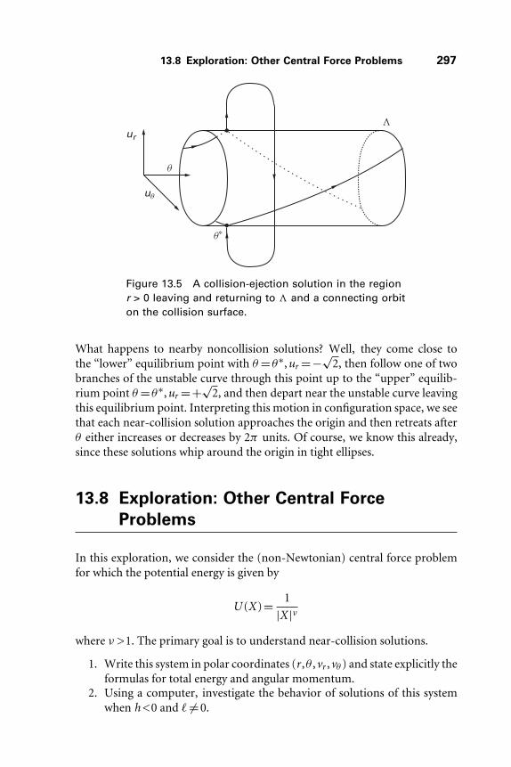
13.8 Exploration: Other Central Force Problems 297
D
h
uh
ur
h∗
Figure 13.5 A collision-ejection solution in the regionr > 0 leaving and returning to � and a connecting orbiton the collision surface.
What happens to nearby noncollision solutions? Well, they come close tothe “lower” equilibrium point with θ =θ∗,ur =−√
2, then follow one of twobranches of the unstable curve through this point up to the “upper” equilib-rium point θ =θ∗,ur =+√
2, and then depart near the unstable curve leavingthis equilibrium point. Interpreting this motion in configuration space, we seethat each near-collision solution approaches the origin and then retreats afterθ either increases or decreases by 2π units. Of course, we know this already,since these solutions whip around the origin in tight ellipses.
13.8 Exploration: Other Central Force
Problems
In this exploration, we consider the (non-Newtonian) central force problemfor which the potential energy is given by
U (X)= 1
|X |ν
where ν >1. The primary goal is to understand near-collision solutions.
1. Write this system in polar coordinates (r ,θ ,vr ,vθ ) and state explicitly theformulas for total energy and angular momentum.
2. Using a computer, investigate the behavior of solutions of this systemwhen h<0 and � �=0.

298 Chapter 13 Applications in Mechanics
3. Blow up the singularity at the origin via the change of variables
ur = rν/2vr , uθ = rν/2vθ
and an appropriate change of timescale and write down the new system.4. Compute the vector field on the collision surface � determined in r =0
by the total energy relation.5. Describe the bifurcation that occurs on � when ν =2.6. Describe the structure of �h,� for all ν >1.7. Describe the change of structure of �h,� that occurs when ν passes
through the value 2.8. Describe the behavior of solutions in �h,� when ν >2.9. Suppose 1<ν <2. Describe the behavior of solutions as they pass close
to the singularity at the origin.10. Using the fact that solutions of this system are preserved by rotations
about the origin, describe the behavior of solutions in �h,� when h<0and � �=0.
13.9 Exploration: Classical Limits of
Quantum Mechanical Systems
In this exploration we investigate the anisotropic Kepler problem. This is aclassical mechanical system with two degrees of freedom that depends on aparameter μ. When μ=1 the system reduces to the Newtonian central forcesystem discussed in Section 13.4. When μ>1 some anisotropy is introducedinto the system, so that we no longer have a central force field. We still havesome collision-ejection orbits, as in the central force system, but the behaviorof nearby orbits is quite different from those when μ=1.
The anisotropic Kepler problem was first introduced by Gutzwiller as aclassical mechanical approximation to certain quantum mechanical systems.In particular, this system arises naturally when one looks for bound states of anelectron near a donor impurity of a semiconductor. Here the potential is dueto an ordinary Coulomb field, while the kinetic energy becomes anisotropicbecause of the electronic band structure in the solid. Equivalently, we can viewthis system as having an anisotropic potential energy function. Gutzwillersuggests that this situation is akin to an electron whose mass in one directionis larger than in other directions. For more background on the quantummechanical applications of this work, refer to [22].
The anisotropic Kepler system is given by
x ′′ = −μx
(μx2+y2)3/2

Exercises 299
y ′′ = −y
(μx2+y2)3/2
where μ is a parameter that we assume is greater than 1.
1. Show that this system is conservative with potential energy given by
U (x ,y)= −1√μx2+y2
and write down an explicit formula for total energy.2. Describe the geometry of the energy surface �h for energy h<0.3. Restricting to the case of negative energy, show that the only solutions
that meet the zero velocity curve and are straight-line collision-ejectionorbits for the system lie on the x- and y-axes in configuration space.
4. Show that angular momentum is no longer an integral for this system.5. Rewrite this system in polar coordinates.6. Using a change of variables and time rescaling as for the Newtonian
central force problem (Section 13.7), blow up the singularity and writedown a new system without any singularities at r =0.
7. Describe the structure of the collision surface � (the intersection of �h
with r =0 in the scaled coordinates). In particular, why would someonecall this surface a “bumpy torus?”
8. Find all equilibrium points on � and determine the eigenvalues of thelinearized system at these points. Determine which equilibria on � aresinks, sources, and saddles.
9. Explain the bifurcation that occurs on � when μ=9/8.10. Find a function that is nondecreasing along all nonequilibrium solutions
in �.11. Determine the fate of the stable and unstable curves of the saddle points
in the collision surface. Hint: Rewrite the equation on this surface toeliminate time and estimate the slope of solutions as they climb up �.
12. When μ>9/8, describe in qualitative terms what happens to solutionsthat approach collision close to the collision-ejection orbits on the x-axis.In particular, how do they retreat from the origin in the configurationspace? How do solutions approach collision when traveling near they-axis?
E X E R C I S E S
1. Which of the following force fields on R2 are conservative?
(a) F(x , y)= (−x2, −2y2)

300 Chapter 13 Applications in Mechanics
(b) F(x , y)= (x2−y2, 2xy)
(c) F(x , y)= (x , 0)
2. Prove that the equation
1
r= 1
h(1+ε cosθ)
determines a hyperbola, parabola, and ellipse when ε >1, ε =1, andε <1, respectively.
3. Consider the case of a particle moving directly away from the origin attime t =0 in the Newtonian central force system. Find a specific formulafor this solution and discuss the corresponding motion of the particle. Forwhich initial conditions does the particle eventually reverse direction?
4. In the Newtonian central force system, describe the geometry of �h,�
when h>0 and h =0.5. Let F(X) be a force field on R3. Let X0, X1 be points in R3 and let Y (s)
be a path in R3 with s0 ≤ s ≤ s1, parametrized by arc length s, from X0 toX1. The work done in moving a particle along this path is defined to bethe integral ∫ s1
s0
F(y(s))·y ′(s)ds
where Y ′(s) is the (unit) tangent vector to the path. Prove that the forcefield is conservative if and only if the work is independent of the path. Infact, if F =−grad V , then the work done is V (X1)−V (X0).
6. Describe solutions to the non-Newtonian central force system given by
X ′′ =− X
|X |4 .
7. Discuss solutions of the equation
X ′′ = X
|X |3 .
This equation corresponds to a repulsive rather than attractive force atthe origin.
8. This and the next two problems deal with the two-body problem. Let thepotential energy be
U = gm1m2
|X2−X1|
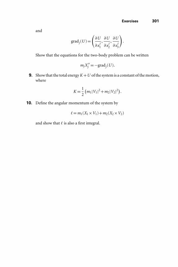
Exercises 301
and
gradj(U )=(
∂U
∂xj1
,∂U
∂xj2
,∂U
∂xj3
).
Show that the equations for the two-body problem can be written
mjX′′j =−gradj(U ).
9. Show that the total energy K +U of the system is a constant of the motion,where
K = 1
2
(m1|V1|2+m2|V2|2
).
10. Define the angular momentum of the system by
�=m1(X1×V1)+m2(X2×V2)
and show that � is also a first integral.

This Page Intentionally Left Blank

14The Lorenz System
So far, in all of the differential equations we have studied, we have not encoun-tered any “chaos.” The reason is simple: The linear systems of the first fewchapters always exhibit straightforward, predictable behavior. (OK, we maysee solutions wrap densely around a torus as in the oscillators of Chapter 6, butthis is not chaos.) Also, for the nonlinear planar systems of the last few chap-ters, the Poincaré-Bendixson theorem completely eliminates any possibility ofchaotic behavior. So, to find chaotic behavior, we need to look at nonlinear,higher dimensional systems.
In this chapter we investigate the system that is, without doubt, the mostfamous of all chaotic differential equations, the Lorenz system from meteo-rology. First formulated in 1963 by E. N. Lorenz as a vastly oversimplifiedmodel of atmospheric convection, this system possesses what has come tobe known as a “strange attractor.” Before the Lorenz model started makingheadlines, the only types of stable attractors known in differential equationswere equilibria and closed orbits. The Lorenz system truly opened up newhorizons in all areas of science and engineering, because many of the phe-nomena present in the Lorenz system have later been found in all of theareas we have previously investigated (biology, circuit theory, mechanics, andelsewhere).
In the ensuing 40 years, much progress has been made in the study ofchaotic systems. Be forewarned, however, that the analysis of the chaoticbehavior of particular systems like the Lorenz system is usually extremelydifficult. Most of the chaotic behavior that is readily understandable arisesfrom geometric models for particular differential equations, rather than from
303

304 Chapter 14 The Lorenz System
the actual equations themselves. Indeed, this is the avenue we pursue here. Wewill present a geometric model for the Lorenz system that can be completelyanalyzed using tools from discrete dynamics. Although this model has beenknown for some 30 years, it is interesting to note the fact that this model wasonly shown to be equivalent to the Lorenz system in the year 1999.
14.1 Introduction to the Lorenz System
In 1963, E. N. Lorenz [29] attempted to set up a system of differential equationsthat would explain some of the unpredictable behavior of the weather. Mostviable models for weather involve partial differential equations; Lorenz soughta much simpler and easier-to-analyze system.
The Lorenz model may be somewhat inaccurately thought of as follows.Imagine a planet whose “atmosphere” consists of a single fluid particle. As onearth, this particle is heated from below (and hence rises) and cooled fromabove (so then falls back down). Can a weather expert predict the “weather”on this planet? Sadly, the answer is no, which raises a lot of questions aboutthe possibility of accurate weather prediction down here on earth, where wehave quite a few more particles in our atmosphere.
A little more precisely, Lorenz looked at a two-dimensional fluid cell thatwas heated from below and cooled from above. The fluid motion can bedescribed by a system of differential equations involving infinitely many vari-ables. Lorenz made the tremendous simplifying assumption that all but threeof these variables remained constant. The remaining independent variablesthen measured, roughly speaking, the rate of convective “overturning” (x),and the horizontal and vertical temperature variation (y and z , respectively).The resulting motion led to a three-dimensional system of differential equa-tions that involved three parameters: the Prandtl number σ , the Rayleighnumber r , and another parameter b that is related to the physical size of thesystem. When all of these simplifications were made, the system of differentialequations involved only two nonlinear terms and was given by
x ′ = σ (y − x)
y ′ = rx − y − xz
z ′ = xy − bz .
In this system all three parameters are assumed to be positive and, moreover,σ > b + 1. We denote this system by X ′ = L(X). In Figure 14.1, we havedisplayed the solution curves through two different initial conditions P1 =(0, 2, 0) and P2 = (0, −2, 0) when the parameters are σ = 10, b = 8/3, and

14.1 Introduction to the Lorenz System 305
x
y
z
P1P2
Figure 14.1 The Lorenz attractor. Two solutions with initial conditions P1 =(0, 2, 0) and P2 = (0, −2, 0).
r = 28. These are the original parameters that led to Lorenz’s discovery. Notehow both solutions start out very differently, but eventually have more or lessthe same fate: They both seem to wind around a pair of points, alternating attimes which point they encircle. This is the first important fact about the Lorenzsystem: All nonequilibrium solutions tend eventually to the same complicatedset, the so-called Lorenz attractor.
There is another important ingredient lurking in the background here. InFigure 14.1, we started with two relatively far apart initial conditions. Had westarted with two very close initial conditions, we would not have observed the“transient behavior” apparent in Figure 14.1. Rather, more or less the samepicture would have resulted for each solution. This, however, is misleading.When we plot the actual coordinates of the solutions, we see that these twosolutions actually move quite far apart during their journey around the Lorenzattractor. This is illustrated in Figure 14.2, where we have graphed the xcoordinates of two solutions that start out nearby, one at (0, 2, 0), the other (ingray) at (0, 2. 01, 0). These graphs are nearly identical for a certain time period,but then they differ considerably as one solution travels around one of the lobesof the attractor while the other solution travels around the other. No matterhow close two solutions start, they always move apart in this manner whenthey are close to the attractor. This is sensitive dependence on initial conditions,one of the main features of a chaotic system.
We will describe in detail the concept of an attractor and chaos in thischapter. But first, we need to investigate some of the more familiar features ofthe system.
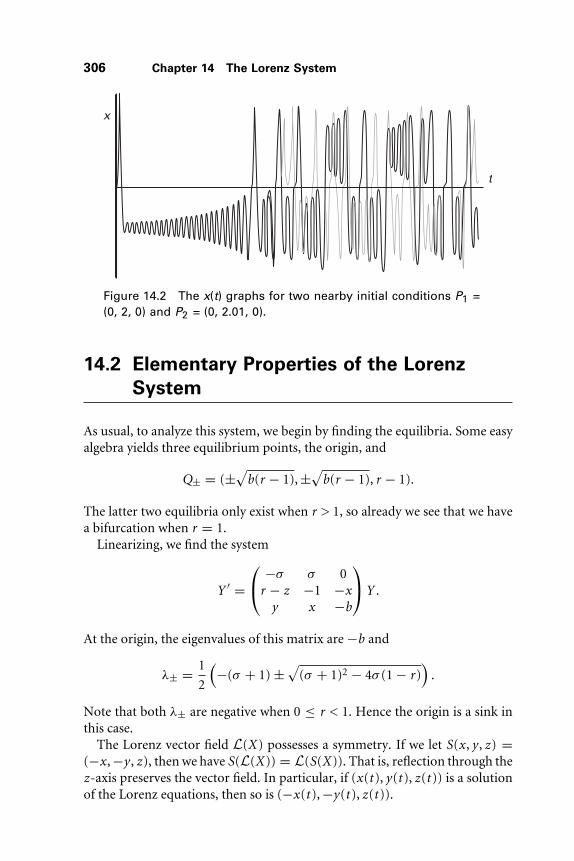
306 Chapter 14 The Lorenz System
x
t
Figure 14.2 The x(t) graphs for two nearby initial conditions P1 =(0, 2, 0) and P2 = (0, 2.01, 0).
14.2 Elementary Properties of the Lorenz
System
As usual, to analyze this system, we begin by finding the equilibria. Some easyalgebra yields three equilibrium points, the origin, and
Q± = (±√
b(r − 1), ±√
b(r − 1), r − 1).
The latter two equilibria only exist when r > 1, so already we see that we havea bifurcation when r = 1.
Linearizing, we find the system
Y ′ =⎛⎝ −σ σ 0
r − z −1 −xy x −b
⎞⎠Y .
At the origin, the eigenvalues of this matrix are −b and
λ± = 1
2
(−(σ + 1) ±
√(σ + 1)2 − 4σ (1 − r)
).
Note that both λ± are negative when 0 ≤ r < 1. Hence the origin is a sink inthis case.
The Lorenz vector field L(X) possesses a symmetry. If we let S(x , y , z) =(−x , −y , z), then we have S(L(X)) = L(S(X)). That is, reflection through thez-axis preserves the vector field. In particular, if (x(t ), y(t ), z(t )) is a solutionof the Lorenz equations, then so is (−x(t ), −y(t ), z(t )).

14.2 Elementary Properties of the Lorenz System 307
When x = y = 0, we have x ′ = y ′ = 0, so the z-axis is invariant. On thisaxis, we have simply z ′ = −bz , so all solutions tend to the origin on this axis.In fact, the solution through any point in R3 tends to the origin when r < 1,for we have:
Proposition. Suppose r < 1. Then all solutions of the Lorenz system tend tothe equilibrium point at the origin.
Proof: We construct a strict Liapunov function on all of R3. Let
L(x , y , z) = x2 + σ y2 + σ z2.
Then we have
L = −2σ(x2 + y2 − (1 + r)xy
) − 2σbz2.
We therefore have L < 0 away from the origin provided that
g (x , y) = x2 + y2 − (1 + r)xy > 0
for (x , y) �= (0, 0). This is clearly true along the y-axis. Along any other straightline y = mx in the xy-plane we have
g (x , mx) = x2(m2 − (1 + r)m + 1).
But the quadratic term m2 − (1 + r)m + 1 is positive for all m if r < 1, as iseasily checked. Hence g (x , y) > 0 for (x , y) �= (0, 0). �
When r increases through 1, two things happen. First, the eigenvalue λ+at the origin becomes positive, so the origin is now a saddle with a two-dimensional stable surface and an unstable curve. Second, the two equilibriaQ± are born at the origin when r = 1 and move away as r increases.
Proposition. The equilibrium points Q± are sinks provided
1 < r < r∗ = σ
(σ + b + 3
σ − b − 1
).
Proof: From the linearization, we calculate that the eigenvalues at Q± satisfythe cubic polynomial
fr (λ) = λ3 + (1 + b + σ )λ2 + b(σ + r)λ + 2bσ (r − 1) = 0.

308 Chapter 14 The Lorenz System
When r = 1 the polynomial f1 has distinct roots at 0, −b, and −σ − 1. Theseroots are distinct since σ > b + 1 so that
−σ − 1 < −σ + 1 < −b < 0.
Hence for r close to but greater than 1, fr has three real roots close to thesevalues. Note that fr (λ) > 0 for λ ≥ 0 and r > 1. Looking at the graph of fr ,it follows that, at least for r close to 1, the three roots of fr must be real andnegative.
We now let r increase and ask what is the lowest value of r for which fr hasan eigenvalue with zero real part. Note that this eigenvalue must in fact be ofthe form ±iω with ω �= 0, since fr is a real polynomial that has no roots equalto 0 when r > 1. Solving fr (iω) = 0 by equating both real and imaginary partsto zero then yields the result (recall that we have assumed σ > b + 1). �
We remark that a Hopf bifurcation is known to occur at r∗, but proving thisis beyond the scope of this book.
When r > 1 it is no longer true that all solutions tend to the origin. However,we can say that solutions that start far from the origin do at least move closerin. To be precise, let
V (x , y , z) = rx2 + σ y2 + σ (z − 2r)2.
Note that V (x , y , z) = ν > 0 defines an ellipsoid in R3 centered at (0, 0, 2r).We will show:
Proposition. There exists ν∗ such that any solution that starts outside theellipsoid V = ν∗ eventually enters this ellipsoid and then remains trapped thereinfor all future time.
Proof: We compute
V = −2σ(rx2 + y2 + b(z2 − 2rz)
)= −2σ
(rx2 + y2 + b(z − r)2 − br2).
The equation
rx2 + y2 + b(z − r)2 = μ
also defines an ellipsoid when μ > 0. When μ > br2 we have V < 0. Thuswe may choose ν∗ large enough so that the ellipsoid V = ν∗ strictly contains

14.2 Elementary Properties of the Lorenz System 309
the ellipsoid
rx2 + y2 + b(z − r)2 = br2
in its interior. Then V < 0 for all ν ≥ ν∗. �
As a consequence, all solutions starting far from the origin are attracted to aset that sits inside the ellipsoid V = ν∗. Let � denote the set of all points whosesolutions remain for all time (forward and backward) in this ellipsoid. Thentheω-limit set of any solution of the Lorenz system must lie in�. Theoretically,� could be a large set, perhaps bounding an open region in R3. However, forthe Lorenz system, this is not the case.
To see this, recall from calculus that the divergence of a vector field F(X) onR3 is given by
div F =3∑
i=1
∂Fi
∂xi(X).
The divergence of F measures how fast volumes change under the flow φt of F .Suppose D is a region in R3 with a smooth boundary, and let D(t ) = φt (D),the image of D under the time t map of the flow. Let V (t ) be the volume ofD(t ). Then Liouville’s theorem asserts that
dV
dt=
∫D(t )
div F dx dy dz .
For the Lorenz system, we compute immediately that the divergence is theconstant −(σ + 1 + b) so that volume decreases at a constant rate
dV
dt= −(σ + 1 + b)V .
Solving this simple differential equation yields
V (t ) = e−(σ+1+b)t V (0)
so that any volume must shrink exponentially fast to 0. In particular, we have:
Proposition. The volume of � is zero. �
The natural question is what more can we say about the structure of the“attractor” �? In dimension two, such a set would consist of a collection of

310 Chapter 14 The Lorenz System
limit cycles, equilibrium points, and solutions connecting them. In higherdimensions, these attractors may be much “stranger,” as we show in the nextsection.
14.3 The Lorenz Attractor
The behavior of the Lorenz system as the parameter r increases is the subjectof much contemporary research; we are decades (if not centuries) away fromrigorously understanding all of the fascinating dynamical phenomena thatoccur as the parameters change. Sparrow has written an entire book devotedto this subject [44].
In this section we will deal with one specific set of parameters where theLorenz system has an attractor. Roughly speaking, an attractor for the flow isan invariant set that “attracts” all nearby solutions. To be more precise:
Definition
Let X ′ = F(X) be a system of differential equations in Rn withflow φt . A set � is called an attractor if
1. � is compact and invariant;2. There is an open set U containing � such that for each X ∈ U ,
φt (X) ∈ U for all t ≥ 0 and ∩t≥0φt (U ) = �;3. (Transitivity) Given any points Y1, Y2 ∈ � and any open neigh-
borhoods Uj about Yj in U , there is a solution curve thatbegins in U1 and later passes through U2.
The transitivity condition in this definition may seem a little strange.Basically, we include it to guarantee that we are looking at a single attrac-tor rather than a collection of dynamically different attractors. For example,the transitivity condition rules out situations such as that given by the planarsystem
x ′ = x − x3
y ′ = −y .
The phase portrait of this system is shown in Figure 14.3. Note that anysolution of this system enters the set marked U and then tends to one of thethree equilibrium points: either to one of the sinks at (±1, 0) or to the saddle(0, 0). The forward intersection of the flow φt applied to U is the interval−1 ≤ x ≤ 1. This interval meets conditions 1 and 2 in the definition, but

14.3 The Lorenz Attractor 311
U
Figure 14.3 The interval onthe x-axis between the twosinks is not an attractor forthis system, despite the factthat all solutions enter U.
condition 3 is violated, because none of the solution curves passes close topoints in both the left and right half of this interval. We choose not to considerthis set an attractor since most solutions tend to one of the two sinks. We reallyhave two distinct attractors in this case.
As a remark, there is no universally accepted definition of an attractor inmathematics; some people choose to say that a set� that meets only conditions1 and 2 is an attractor, while if � also meets condition 3, it would be called atransitive attractor. For planar systems, condition 3 is usually easily verified;in higher dimensions, however, this can be much more difficult, as we shallsee.
For the rest of this chapter, we restrict attention to the very special case of theLorenz system where the parameters are given by σ = 10, b = 8/3, and r = 28.Historically, these are the values Lorenz used when he first encountered chaoticphenomena in this system. Thus, the specific Lorenz system we consider is
X ′ = L(X) =⎛⎝ 10(y − x)
28x − y − xzxy − (8/3)z
⎞⎠ .
As in the previous section, we have three equilibria: the origin and Q± =(±6
√2, ±6
√2, 27). At the origin we find eigenvalues λ1 = −8/3 and
λ± = −11
2±
√1201
2.
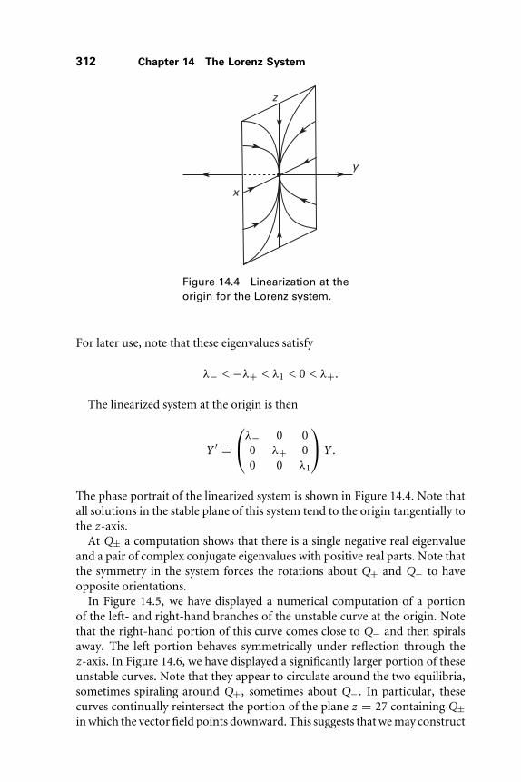
312 Chapter 14 The Lorenz System
x
z
y
Figure 14.4 Linearization at theorigin for the Lorenz system.
For later use, note that these eigenvalues satisfy
λ− < −λ+ < λ1 < 0 < λ+.
The linearized system at the origin is then
Y ′ =⎛⎝λ− 0 0
0 λ+ 00 0 λ1
⎞⎠Y .
The phase portrait of the linearized system is shown in Figure 14.4. Note thatall solutions in the stable plane of this system tend to the origin tangentially tothe z-axis.
At Q± a computation shows that there is a single negative real eigenvalueand a pair of complex conjugate eigenvalues with positive real parts. Note thatthe symmetry in the system forces the rotations about Q+ and Q− to haveopposite orientations.
In Figure 14.5, we have displayed a numerical computation of a portionof the left- and right-hand branches of the unstable curve at the origin. Notethat the right-hand portion of this curve comes close to Q− and then spiralsaway. The left portion behaves symmetrically under reflection through thez-axis. In Figure 14.6, we have displayed a significantly larger portion of theseunstable curves. Note that they appear to circulate around the two equilibria,sometimes spiraling around Q+, sometimes about Q−. In particular, thesecurves continually reintersect the portion of the plane z = 27 containing Q±in which the vector field points downward. This suggests that we may construct

14.3 The Lorenz Attractor 313
Q �
Q�
(0, 0, 0)
Figure 14.5 The unstable curve at the origin.
a Poincaré map on a portion of this plane. As we have seen before, computinga Poincaré map is often impossible, and this case is no different. So we willcontent ourselves with building a simplified model that exhibits much of thebehavior we find in the Lorenz system. As we shall see in the following section,this model provides a computable means to assess the chaotic behavior of thesystem.
(0, 0, 0)
Figure 14.6 More of the unstable curve at the origin.

314 Chapter 14 The Lorenz System
14.4 A Model for the Lorenz Attractor
In this section we describe a geometric model for the Lorenz attractor origi-nally proposed by Guckenheimer and Williams [20]. Tucker [46] showed thatthis model does indeed correspond to the Lorenz system for certain parame-ters. Rather than specify the vector field exactly, we give instead a qualitativedescription of its flow, much as we did in Chapter 11. The specific numberswe use are not that important; only their relative sizes matter.
We will assume that our model is symmetric under the reflection (x , y , z) →(−x , −y , z), as is the Lorenz system. We first place an equilibrium point at theorigin in R3 and assume that, in the cube S given by |x|, |y|, |z | ≤ 5, the systemis linear. Rather than use the eigenvalues λ1 and λ± from the actual Lorenzsystem, we simplify the computations a bit by assuming that the eigenvaluesare −1, 2, and −3, and that the system is given in the cube by
x ′ = −3x
y ′ = 2y
z ′ = −z .
Note that the phase portrait of this system agrees with that in Figure 14.4 andthat the relative magnitudes of the eigenvalues are the same as in the Lorenzcase.
We need to know how solutions make the transit near (0, 0, 0). Consider arectangle R1 in the plane z = 1 given by |x| ≤ 1, 0 < y ≤ ε < 1. As timemoves forward, all solutions that start in R1 eventually reach the rectangle R2
in the plane y = 1 defined by |x| ≤ 1, 0 < z ≤ 1. Hence we have a functionh : R1 → R2 defined by following solution curves as they pass from R1 toR2. We leave it as an exercise to check that this function assumes the form
h
(xy
)=
(x1
z1
)=
(xy3/2
y1/2
).
It follows that h takes lines y = c in R1 to lines z = c1/2 in R2. Also, sincex1 = xz3
1 , we have that h maps lines x = c to curves of the form x1 = cz31 .
Each of these image curves meet the xy–plane perpendicularly, as depicted inFigure 14.7.
Mimicking the Lorenz system, we place two additional equilibria in theplane z = 27, one at Q− = (−10, −20, 27) and the other at Q+ = (10, 20, 27).We assume that the lines given by y = ±20, z = 27 form portions of the stablelines at Q±, and that the other two eigenvalues at these points are complexwith positive real part.
Let � denote the square |x|, |y| ≤ 20, z = 27. We assume that the vectorfield points downward in the interior of this square. Hence solutions spiral

14.4 A Model for the Lorenz Attractor 315
h(x, y)
(x, y)
x
z
y
1
2
Figure 14.7 Solutions making the transitnear (0, 0, 0).
away from Q± in the same manner as in the Lorenz system. We also assumethat the stable surface of (0, 0, 0) first meets � in the line of intersection of thexz–plane and �.
Let ζ± denote the two branches of the unstable curve at the origin. Weassume that these curves make a passage around � and then enter this squareas shown in Figure 14.8. We denote the first point of intersection of ζ± with� by ρ± = (±x∗, ∓y∗).
Q�
Q�Φ(∑�)
Φ(∑�)∑�
∑�p�
f�f�
p�
z
y
x
Figure 14.8 The solutions ζ± and their intersection with � in the modelfor the Lorenz attractor.

316 Chapter 14 The Lorenz System
Now consider a straight line y = ν in �. If ν = 0, all solutions beginningat points on this line tend to the origin as time moves forward. Hence thesesolutions never return to �. We assume that all other solutions originating in� do return to � as time moves forward. How these solutions return leads toour major assumptions about this model:
1. Return condition: Let �+ = � ∩ {y > 0} and �− = � ∩ {y < 0}. Weassume that the solutions through any point in �± return to � in forwardtime. Hence we have a Poincaré map � : �+ ∪ �− → �. We assumethat the images �(�±) are as depicted in Figure 14.8. By symmetry, wehave �(x , y) = −�(−x , −y).
2. Contracting direction: For each ν �= 0 we assume that � maps the liney = ν in � into the line y = g (ν) for some function g . Moreover weassume that � contracts this line in the x direction.
3. Expanding direction: We assume that � stretches �+ and �− in the ydirection by a factor strictly greater than
√2, so that g ′(y) >
√2.
4. Hyperbolicity condition: Besides the expansion and contraction, we assumethat D� maps vectors tangent to �± whose slopes are ±1 to vectors whoseslopes have magnitude larger than μ > 1.
Analytically, these assumptions imply that the map � assumes the form
�(x , y) = (f (x , y), g (y))
where g ′(y) >√
2 and 0 < ∂f /∂x < c < 1. The hyperbolicity condition impliesthat
g ′(y) > μ
∣∣∣∣∂f
∂x± ∂f
∂y
∣∣∣∣.Geometrically, this condition implies that the sectors in the tangent planesgiven by |y| ≥ |x| are mapped by D� strictly inside a sector with steeperslopes. Note that this condition holds if |∂f /∂y| and c are sufficiently smallthroughout �±.
Technically, �(x , 0) is not defined, but we do have
limy→0± �(x , y) = ρ±
where we recall that ρ± is the first point of intersection of ζ± with �. We callρ± the tip of �(�±). In fact, our assumptions on the eigenvalues guaranteethat g ′(y) → ∞ as y → 0 (see Exercise 3 at the end of this chapter).
To find the attractor, we may restrict attention to the rectangle R ⊂ � givenby |y| ≤ y∗, where we recall that ∓y∗ is the y coordinate of the tips ρ±. LetR± = R∩�±. It is easy to check that any solution starting in the interior of �±
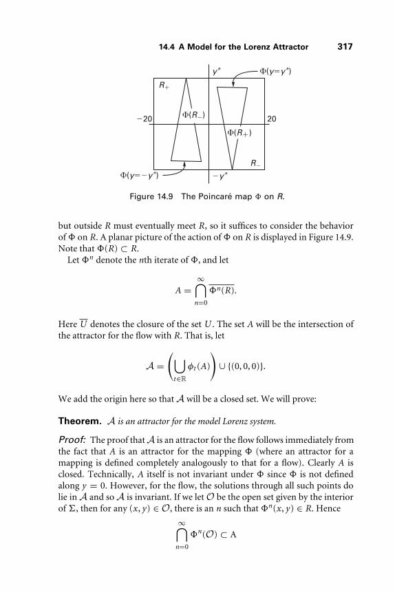
14.4 A Model for the Lorenz Attractor 317
�20 20
y*
�y*
R�
R�
(R�)
(R�)
(y��y*)
(y�y*)
Figure 14.9 The Poincaré map � on R.
but outside R must eventually meet R, so it suffices to consider the behaviorof � on R. A planar picture of the action of � on R is displayed in Figure 14.9.Note that �(R) ⊂ R.
Let �n denote the nth iterate of �, and let
A =∞⋂
n=0
�n(R).
Here U denotes the closure of the set U . The set A will be the intersection ofthe attractor for the flow with R. That is, let
A =(⋃
t∈R
φt (A)
)∪ {(0, 0, 0)}.
We add the origin here so that A will be a closed set. We will prove:
Theorem. A is an attractor for the model Lorenz system.
Proof: The proof that A is an attractor for the flow follows immediately fromthe fact that A is an attractor for the mapping � (where an attractor for amapping is defined completely analogously to that for a flow). Clearly A isclosed. Technically, A itself is not invariant under � since � is not definedalong y = 0. However, for the flow, the solutions through all such points dolie in A and so A is invariant. If we let O be the open set given by the interiorof �, then for any (x , y) ∈ O, there is an n such that �n(x , y) ∈ R. Hence
∞⋂n=0
�n(O) ⊂ A

318 Chapter 14 The Lorenz System
By definition, A = ∩n≥0�n(R), and so A = ∩n≥0�
n(O) as well. Thereforeconditions 1 and 2 in the definition of an attractor hold for �.
It remains to show the transitivity property. We need to show that if P1 andP2 are points in A, and Wj are open neighborhoods of Pj in O, then thereexists an n ≥ 0 such that �n(W1) ∩ W2 �= ∅.
Given a set U ⊂ R, let �y(U ) denote the projection of U onto the y-axis.Also let �y(U ) denote the length of �y(U ), which we call the y length of U . Inthe following, U will be a finite collection of connected sets, so �y(U ) is welldefined.
We need a lemma. �
Lemma. For any open set W ⊂ R, there exists n > 0 such that �y(�n(W )) isthe interval [−y∗, y∗]. Equivalently, �n(W ) meets each line y = c in R.
Proof: First suppose that W contains a connected subset W ′ that extendsfrom one of the tips to y = 0. Hence �y(W ′) = y∗. Then �(W ′) is connectedand we have �y(�(W ′)) >
√2y∗. Moreover, �(W ′) also extends from one of
the tips, but now crosses y = 0 since its y length exceeds y∗.Now apply � again. Note that �2(W ′) contains two pieces, one of which
extends to ρ+, the other to ρ−. Moreover, �y(�2(W ′)) > 2y∗. Thus it followsthat �y(�2(W ′)) = [−y∗, y∗] and so we are done in this special case.
For the general case, suppose first that W is connected and does not crossy = 0. Then we have �y(�(W )) >
√2�y(W ) as above, so the y length of
�(W ) grows by a factor of more than√
2.If W does cross y = 0, then we may find a pair of connected sets W ±
with W ± ⊂ {R± ∩ W } and �y(W + ∪ W −) = �y(W ). The images �(W ±)extend to the tips ρ±. If either of these sets also meets y = 0, then weare done by the above. If neither �(W +) nor �(W −) crosses y = 0,then we may apply � again. Both �(W +) and �(W −) are connected sets,and we have �y(�2(W ±)) > 2�y(W ±). Hence for one of W + or W −we have �y(�2(W ±)) > �y(W ) and again the y length of W grows underiteration.
Thus if we continue to iterate � or �2 and choose the appropriate largestsubset of �j(W ) at each stage as above, then we see that the y lengthsof these images grow without bound. This completes the proof of thelemma. �
We now complete the proof of the theorem. We must find a point inW1 whose image under an iterate of � lies in W2. Toward that end, notethat ∣∣∣�k(x1, y) − �k(x2, y)
∣∣∣ ≤ ck |x1 − x2|

14.5 The Chaotic Attractor 319
since �j(x1, y) and �j(x2, y) lie on the same straight line parallel to the x-axisfor each j and � contracts distances in the x direction by a factor of c < 1.
We may assume that W2 is a disk of diameter ε. Recalling that the width of Rin the x direction is 40, we choose m such that 40cm < ε. Consider �−m(P2).Note that �−m(P2) is defined since P2 ∈ ∩n≥0�
n(R). Say �−m(P2) = (ξ , η).From the lemma, we know that there exists n such that
�y(�n(W1)) = [−y∗, y∗].
Hence we may choose a point (ξ1, η) ∈ �n(W1). Say (ξ1, η) = �n(x , y) where(x , y) ∈ W1, so that �n(x , y) and �−m(P2) have the same y coordinate. Thenwe have
|�m+n(x , y) − P2| = |�m(ξ1, η) − P2|= |�m(ξ1, η) − �m(ξ , η)|≤ 40cm < ε.
We have found a point (x , y) ∈ W1 whose solution passes through W2. Thisconcludes the proof. �
Note that, in the above proof, the solution curve that starts near P1 andcomes close to P2 need not lie in the attractor. However, it is possible to findsuch a solution that does lie in A (see Exercise 4).
14.5 The Chaotic Attractor
In the previous section we reduced the study of the behavior of solutions ofthe Lorenz system to the analysis of the dynamics of the Poincaré map �.In the process, we dropped from a three-dimensional system of differentialequations to a two-dimensional mapping. But we can do better. Accordingto our assumptions, two points that share the same y coordinate in � aremapped to two new points whose y coordinates are given by g (y) and henceare again the same. Moreover, the distance between these points is contracted.It follows that, under iteration of �, we need not worry about all points on aline y = constant; we need only keep track of how the y coordinate changesunder iteration of g . Then, as we shall see, the Poincaré map � is completelydetermined by the dynamics of the one-dimensional function g defined on theinterval [−y∗, y∗]. Indeed, iteration of this function completely determines thebehavior of all solutions in the attractor. In this section, we begin to analyze

320 Chapter 14 The Lorenz System
�y* y*
g(�y*)
g(y*)
Figure 14.10 The graph of theone-dimensional function g on I =[−y∗, y∗].
the dynamics of this one-dimensional discrete dynamical system. In Chapter 15,we plunge more deeply into this topic.
Let I be the interval [−y∗, y∗]. Recall that g is defined on I except at y = 0and satisfies g (−y) = −g (y). From the results of the previous section, wehave g ′(y) >
√2, and 0 < g (y∗) < y∗ and −y∗ < g (−y∗) < 0. Also,
limy→0± g (y) = ∓y∗.
Hence the graph of g resembles that shown in Figure 14.10. Note that allpoints in the interval [g (−y∗), g (y∗)] have two preimages, while points in theintervals (−y∗, g (−y∗)) and (g (y∗), y∗) have only one. The endpoints of I ,namely, ±y∗, have no preimages in I since g (0) is undefined.
Let y0 ∈ I . We will investigate the structure of the set A ∩ {y = y0}.We define the (forward) orbit of y0 to be the set (y0, y1, y2, . . .) where yn =g (yn−1) = g n(y0). For each y0, the forward orbit of y0 is uniquely determined,though it terminates if g n(y0) = 0.
A backward orbit of y0 is a sequence of the form (y0, y−1, y−2, . . .) whereg (y−k) = y−k+1. Unlike forward orbits of g , there are infinitely many distinctbackward orbits for a given y0 except in the case where y0 = ±y∗ (since thesetwo points have no preimages in I ). To see this, suppose first that y0 does notlie on the forward orbit of ±y∗. Then each point y−k must have either one ortwo distinct preimages, since y−k �= ±y∗. If y−k has only one preimage y−k−1,then y−k lies in either (−y∗, g (−y∗) or (g (y∗), y∗). But then the graph of gshows that y−k−1 must have two preimages. So no two consecutive points in agiven backward orbit can have only one preimage, and this shows that y0 hasinfinitely many distinct backward orbits.
If we happen to have y−k = ±y∗ for some k > 0, then this backwardorbit stops since ±y∗ has no preimage in I . However, y−k+1 must have two

14.5 The Chaotic Attractor 321
preimages, one of which is the endpoint and the other is a point in I that doesnot equal the other endpoint. Hence we can continue taking preimages of thissecond backward orbit as before, thereby generating infinitely many distinctbackward orbits as before.
We claim that each of these infinite backward orbits of y0 corresponds toa unique point in A ∩ {y = y0}. To see this, consider the line J−k given byy = y−k in R. Then �k(J−k) is a closed subinterval of J0 for each k. Notethat �(J−k−1) ⊂ J−k , since �(y = y−k−1) is a proper subinterval of y =y−k . Hence the nested intersection of the sets �k(J−k) is nonempty, and anypoint in this intersection has backward orbit (y0, y−1, y−2, . . .) by construction.Furthermore, the intersection point is unique, since each application of �
contracts the intervals y = y−k by a factor of c < 1.In terms of our model, we therefore see that the attractor A is a complicated
set. We have proved the following:
Proposition. The attractor A for the model Lorenz system meets each of thelines y = y0 �= y∗ in R infinitely many distinct points. In forward time all of thesolution curves through each point on this line either:
1. Meet the line y = 0, in which case the solution curves all tend to theequilibrium point at (0, 0, 0), or
2. Continually reintersect R, and the distances between these intersection pointson the line y = yk tend to 0 as time increases. �
Now we turn to the dynamics of � in R. We first discuss the behavior ofthe one-dimensional function g , and then use this information to understandwhat happens for �. Given any point y0 ∈ I , note that nearby forward orbitsof g move away from the orbit of y0 since g ′ >
√2. More precisely, we have:
Proposition. Let 0 < ν < y∗. Let y0 ∈ I = [−y∗, y∗]. Given any ε > 0, wemay find u0, v0 ∈ I with |u0 − y0| < ε and |v0 − y0| < ε and n > 0 such that|g n(u0) − g n(v0)| ≥ 2ν.
Proof: Let J be the interval of length 2ε centered at y0. Each iteration of gexpands the length of J by a factor of at least
√2, so there is an iteration for
which g n(J ) contains 0 in its interior. Then g n+1(J ) contains points arbitrarilyclose to both ±y∗, and hence there are points in g n+1(J ) whose distance fromeach other is at least 2ν. This completes the proof. �
Let’s interpret the meaning of this proposition in terms of the attractor A.Given any point in the attractor, we may always find points arbitrarily nearbywhose forward orbits move apart just about as far as they possibly can. This isthe hallmark of a chaotic system: We call this behavior sensitive dependence oninitial conditions. A tiny change in the initial position of the orbit may result in

322 Chapter 14 The Lorenz System
drastic changes in the eventual behavior of the orbit. Note that we must have asimilar sensitivity for the flow in A; certain nearby solution curves in A mustalso move far apart. This is the behavior we witnessed in Figure 14.2.
This should be contrasted with the behavior of points in A that lie on thesame line y = constant with −y∗ < y < y∗. As we saw previously, there areinfinitely many such points in A. Under iteration of �, the successive imagesof all of these points move closer together rather than separating.
Recall now that a subset of I is dense if its closure is all of I . Equivalently, asubset of I is dense if there are points in the subset arbitrarily close to any pointwhatsoever in I . Also, a periodic point for g is a point y0 for which g n(y0) = y0
for some n > 0. Periodic points for g correspond to periodic solutions of theflow.
Proposition. The periodic points of g are dense in I .
Proof: As in the proof that A is an attractor in the last section, given anysubinterval J of I − {0}, we may find n so that g n maps some subintervalJ ′ ⊂ J in one-to-one fashion over either (−y∗, 0] or [0, y∗). Thus either g n(J ′)contains J ′, or the next iteration, g n+1(J ′), contains J ′. In either case, thegraphs of g n or g n+1 cross the diagonal line y = x over J ′. This yields aperiodic point for g in J . �
Now let us interpret this result in terms of the attractor A. We claim thatperiodic points for � are also dense in A. To see this, let P ∈ A and U be anopen neighborhood of P . We assume that U does not cross the line y = 0(otherwise just choose a smaller neighborhood nearby that is disjoint fromy = 0). For small enough ε > 0, we construct a rectangle W ⊂ U centered atP and having width 2ε (in the x direction) and height ε (in the y direction).
Let W1 ⊂ W be a smaller square centered at P with sidelength ε/2. Bythe transitivity result of the previous section, we may find a point Q1 ∈ W1
such that �n(Q1) = Q2 ∈ W1. By choosing a subset of W1 if necessary, wemay assume that n > 4 and furthermore that n is so large that cn < ε/8. Itfollows that the image of �n(W ) (not �n(W1)) crosses through the interiorof W nearly vertically and extends beyond its top and bottom boundaries, asdepicted in Figure 14.11. This fact uses the hyperbolicity condition.
Now consider the lines y = c in W . These lines are mapped to other suchlines in R by �n . Since the vertical direction is expanded, some of the linesmust be mapped above W and some below. It follows that one such line y = c0
must be mapped inside itself by �n , and therefore there must be a fixed pointfor �n on this line. Since this line is contained in W , we have produced aperiodic point for � in W . This proves density of periodic points in A.
In terms of the flow, a solution beginning at a periodic point of � is a closedorbit. Hence the set of points lying on closed orbits is a dense subset of A. The

14.5 The Chaotic Attractor 323
W
W1
Q1 Q2
P
y�c0(y�c0)
n(W )
Figure 14.11 � maps W acrossitself.
structure of these closed orbits is quite interesting from a topological point ofview, because many of these closed curves are actually “knotted.” See [9] andExercise 10.
Finally, we say that a function g is transitive on I if, for any pair of points y1
and y2 in I and neighborhoods Ui of yi , we can find y ∈ U1 and n such thatg n(y) ∈ U2. Just as in the proof of density of periodic points, we may use thefact that g is expanding in the y direction to prove:
Proposition. The function g is transitive on I .
We leave the details to the reader. In terms of �, we almost proved thecorresponding result when we showed that A was an attractor. The only detailwe did not provide was the fact that we could find a point in A whose orbitmade the transit arbitrarily close to any given pair of points in A. For thisdetail, we refer to Exercise 4.
Thus we can summarize the dynamics of � on the attractor A of the Lorenzmodel as follows.
Theorem. (Dynamics of the Lorenz Model) The Poincaré map �
restricted to the attractor A for the Lorenz model has the following properties:
1. � has sensitive dependence on initial conditions;2. Periodic points of � are dense in A;3. � is transitive on A. �
We say that a mapping with the above properties is chaotic. We caution thereader that, just as in the definition of an attractor, there are many definitions ofchaos around. Some involve exponential separation of orbits, others involvepositive Liapunov exponents, and others do not require density of periodicpoints. It is an interesting fact that, for continuous functions of the real line,

324 Chapter 14 The Lorenz System
density of periodic points and transitivity are enough to guarantee sensitivedependence. See [8]. We will delve more deeply into chaotic behavior ofdiscrete systems in the next chapter.
14.6 Exploration: The Rössler Attractor
In this exploration, we investigate a three-dimensional system similar in manyrespects to the Lorenz system. The Rössler system [37] is given by
x ′ = −y − z
y ′ = x + ay
z ′ = b + z(x − c)
where a, b, and c are real parameters. For simplicity, we will restrict attentionto the case where a = 1/4, b = 1, and c ranges from 0 to 7.
As with the Lorenz system, it is difficult to prove specific results about thissystem, so much of this exploration will center on numerical experimentationand the construction of a model.
1. First find all equilibrium points for this system.2. Describe the bifurcation that occurs at c = 1.3. Investigate numerically the behavior of this system as c increases. What
bifurcations do you observe?4. In Figure 14.12 we have plotted a single solution for c = 5. 5. Compute
other solutions for this parameter value, and display the results from other
x
y
z
Figure 14.12 The Rössler attractor.

Exercises 325
viewpoints in R3. What conjectures do you make about the behavior ofthis system?
5. Using techniques described in this chapter, devise a geometric model thatmimics the behavior of the Rössler system for this parameter value.
6. Construct a model mapping on a two-dimensional region whose dynam-ics might explain the behavior observed in this system.
7. As in the Lorenz system, describe a possible way to reduce this functionto a mapping on an interval.
8. Give an explicit formula for this one-dimensional model mapping. Whatcan you say about the chaotic behavior of your model?
9. What other bifurcations do you observe in the Rössler system as c risesabove 5.5?
E X E R C I S E S
1. Consider the system
x ′ = −3x
y ′ = 2y
z ′ = −z .
Recall from Section 14.4 that there is a function h : R1 → R2 whereR1 is given by |x| ≤ 1, 0 < y ≤ ε < 1 and z = 1, and R2 is given by|x| ≤ 1, 0 < z ≤ 1, and y = 1. Show that h is given by
h
(xy
)=
(x1
z1
)=
(xy3/2
y1/2
).
2. Suppose that the roles of x and z are reversed in the previous exercise.That is, suppose x ′ = −x and z ′ = −3z . Describe the image of h(x , y)in R2 in this case.
3. For the Poincaré map �(x , y) = (f (x , y), g (y)) for the model attractor,use the results of Exercise 1 to show that g ′(y) → ∞ as y → 0.
4. Show that it is possible to verify the transitivity condition for the Lorenzmodel with a solution that actually lies in the attractor.
5. Prove that arbitrarily close to any point in the model Lorenz attrac-tor, there is a solution that eventually tends to the equilibrium point at(0, 0, 0).
6. Prove that there is a periodic solution γ of the model Lorenz system thatmeets the rectangle R in precisely two distinct points.
7. Prove that arbitrarily close to any point in the model Lorenz attractor,there is a solution that eventually tends to the periodic solution γ fromthe previous exercise.

326 Chapter 14 The Lorenz System
R
Figure 14.13 � mapsR completely acrossitself.
8. Consider a map � on a rectangle R as shown in Figure 14.13. where �
has properties similar to the model Lorenz �. How many periodic pointsof period n does � have?
9. Consider the system
x ′ = 10(y − x)
y ′ = 28x − y + xz
z ′ = xy − (8/3)z .
Show that this system is not chaotic. (Note the +xz term in the equationfor y ′.) Hint: Show that most solutions tend to ∞.
10. A simple closed curve in R3 is knotted if it cannot be continuouslydeformed into the “unknot,” the unit circle in the xy–plane, withouthaving self-intersections along the way. Using the model Lorenz attrac-tor, sketch a curve that follows the dynamics of � (so should approximatea real solution) and is knotted. (You might want to use some string forthis!)
11. Use a computer to investigate the behavior of the Lorenz system as rincreases from 1 to 28 (with σ = 10 and b = 8/3). Describe in qualitativeterms any bifurcations you observe.

15Discrete Dynamical Systems
Our goal in this chapter is to begin the study of discrete dynamical systems.As we have seen at several stages in this book, it is sometimes possible toreduce the study of the flow of a differential equation to that of an iteratedfunction, namely, a Poincaré map. This reduction has several advantages. Firstand foremost, the Poincaré map lives on a lower dimensional space, whichtherefore makes visualization easier. Secondly, we do not have to integrateto find “solutions” of discrete systems. Rather, given the function, we simplyiterate the function over and over to determine the behavior of the orbit, whichthen dictates the behavior of the corresponding solution.
Given these two simplifications, it then becomes much easier to comprehendthe complicated chaotic behavior that often arises for systems of differentialequations. While the study of discrete dynamical systems is a topic that couldeasily fill this entire book, we will restrict attention here primarily to the portionof this theory that helps us understand chaotic behavior in one dimension. Inthe following chapter we will extend these ideas to higher dimensions.
15.1 Introduction to Discrete Dynamical
Systems
Throughout this chapter we will work with real functions f : R → R. Asusual, we assume throughout that f is C∞, although there will be severalspecial examples where this is not the case.
327

328 Chapter 15 Discrete Dynamical Systems
Let f n denote the nth iterate of f . That is, f n is the n-fold composition of fwith itself. Given x0 ∈ R, the orbit of x0 is the sequence
x0, x1 = f (x0), x2 = f 2(x0), . . . , xn = f n(x0), . . . .
The point x0 is called the seed of the orbit.
Example. Let f (x) = x2 + 1. Then the orbit of the seed 0 is the sequence
x0 = 0
x1 = 1
x2 = 2
x3 = 5
x4 = 26
...
xn = big
xn+1 = bigger
...
and so forth, so we see that this orbit tends to ∞ as n → ∞. �
In analogy with equilibrium solutions of systems of differential equations,fixed points play a central role in discrete dynamical systems. A point x0 iscalled a fixed point if f (x0) = x0. Obviously, the orbit of a fixed point is theconstant sequence x0, x0, x0, . . ..
The analog of closed orbits for differential equations is given by periodicpoints of period n. These are seeds x0 for which f n(x0) = x0 for some n > 0.As a consequence, like a closed orbit, a periodic orbit repeats itself:
x0, x1, . . . , xn−1, x0, x1, . . . , xn−1, x0 . . . .
Periodic orbits of period n are also called n-cycles. We say that the periodicpoint x0 has minimal period n if n is the least positive integer for whichf n(x0) = x0.
Example. The function f (x) = x3 has fixed points at x = 0, ±1. The func-tion g (x) = −x3 has a fixed point at 0 and a periodic point of period 2

15.1 Introduction to Discrete Dynamical Systems 329
at x = ±1, since g (1) = −1 and g (−1) = 1, so g 2(±1) = ±1. Thefunction
h(x) = (2 − x)(3x + 1)/2
has a 3-cycle given by x0 = 0, x1 = 1, x2 = 2, x3 = x0 = 0 . . .. �
A useful way to visualize orbits of one-dimensional discrete dynamicalsystems is via graphical iteration. In this picture, we superimpose the curvey = f (x) and the diagonal line y = x on the same graph. We display the orbitof x0 as follows: Begin at the point (x0, x0) on the diagonal and draw a verticalline to the graph of f , reaching the graph at (x0, f (x0)) = (x0, x1). Then draw ahorizontal line back to the diagonal, ending at (x1, x1). This procedure movesus from a point on the diagonal directly over the seed x0 to a point directlyover the next point on the orbit, x1. Then we continue from (x1, x1): Firstgo vertically to the graph to the point (x1, x2), then horizontally back to thediagonal at (x2, x2). On the x-axis this moves us from x1 to the next pointon the orbit, x2. Continuing, we produce a sequence of pairs of lines, each ofwhich terminates on the diagonal at a point of the form (xn , xn).
In Figure 15.1a, graphical iteration shows that the orbit of x0 tends to thefixed point z0 under iteration of f . In Figure 15.1b, the orbit of x0 under g lieson a 3-cycle: x0, x1, x2, x0, x1, . . ..
As in the case of equilibrium points of differential equations, there aredifferent types of fixed points for a discrete dynamical system. Suppose that x0
is a fixed point for f . We say that x0 is a sink or an attracting fixed point for f ifthere is a neighborhood U of x0 in R having the property that, if y0 ∈ U , then
y�x y�x
x0 x0 x1 x2x1 x2 z0
y�f (x)
y�g (x)
(a) (b)
Figure 15.1 (a) The orbit of x0 tends to the fixed point at z0under iteration of f, while (b) the orbit of x0 lies on a 3-cycleunder iteration of g.

330 Chapter 15 Discrete Dynamical Systems
f n(y0) ∈ U for all n and, moreover, f n(y0) → x0 as n → ∞. Similarly, x0 is asource or a repelling fixed point if all orbits (except x0) leave U under iterationof f . A fixed point is called neutral or indifferent if it is neither attracting norrepelling.
For differential equations, we saw that it was the derivative of the vector fieldat an equilibrium point that determined the type of the equilibrium point. Thisis also true for fixed points, although the numbers change a bit.
Proposition. Suppose f has a fixed point at x0. Then
1. x0 is a sink if |f ′(x0)| < 1;2. x0 is a source if |f ′(x0)| > 1;3. we get no information about the type of x0 if f ′(x0) = ±1.
Proof: We first prove case (1). Suppose |f ′(x0)| = ν < 1. Choose K withν < K < 1. Since f ′ is continuous, we may find δ > 0 so that |f ′(x)| < K for allx in the interval I = [x0 − δ, x0 + δ]. We now invoke the mean value theorem.Given any x ∈ I , we have
f (x) − x0
x − x0= f (x) − f (x0)
x − x0= f ′(c)
for some c between x and x0. Hence we have
|f (x) − x0| < K |x − x0|.It follows that f (x) is closer to x0 than x and so f (x) ∈ I . Applying this resultagain, we have
|f 2(x) − x0| < K |f (x) − x0| < K 2|x − x0|,and, continuing, we find
|f n(x) − x0| < K n|x − x0|,so that f n(x) → x0 in I as required, since 0 < K < 1.
The proof of case (2) follows similarly. In case (3), we note that each of thefunctions
1. f (x) = x + x3;2. g (x) = x − x3;3. h(x) = x + x2
has a fixed point at 0 with f ′(0) = 1. But graphical iteration (Figure 15.2)shows that f has a source at 0; g has a sink at 0; and 0 is attracting from oneside and repelling from the other for the function h. �

15.1 Introduction to Discrete Dynamical Systems 331
f (x)�x�x3 g(x)�x�x3 h(x)�x�x2
Figure 15.2 In each case, the derivative at 0 is 1, but f has a source at 0; ghas a sink; and h has neither.
Note that, at a fixed point x0 for which f ′(x0) < 0, the orbits of nearbypoints jump from one side of the fixed point to the other at each iteration. SeeFigure 15.3. This is the reason why the output of graphical iteration is oftencalled a web diagram.
Since a periodic point x0 of period n for f is a fixed point of f n , we mayclassify these points as sinks or sources depending on whether |(f n)′(x0)| < 1or |(f n)′(x0)| > 1. One may check that (f n)′(x0) = (f n)′(xj) for any otherpoint xj on the periodic orbit, so this definition makes sense (see Exercise 6 atthe end of this chapter).
Example. The function f (x) = x2 − 1 has a 2-cycle given by 0 and −1.One checks easily that (f 2)′(0) = 0 = (f 2)′(−1), so this cycle is a sink.In Figure 15.4, we show a graphical iteration of f with the graph of f 2
superimposed. Note that 0 and −1 are attracting fixed points for f 2. �
X0 Z0
Figure 15.3 Since −1 <f ′(z0) < 0, the orbit of x0“spirals” toward theattracting fixed point at z0 .

332 Chapter 15 Discrete Dynamical Systems
y�x
y�xf(x)
y�xf 2(x)
�1
Figure 15.4 The graphs of f (x) = x2 −1 andf 2 showing that 0 and −1 lie on an attracting2-cycle for f.
15.2 Bifurcations
Discrete dynamical systems undergo bifurcations when parameters are variedjust as differential equations do. We deal in this section with several types ofbifurcations that occur for one-dimensional systems.
Example. Let fc (x) = x2 + c where c is a parameter. The fixed points forthis family are given by solving the equation x2 + c = x , which yields
p± = 1
2±
√1 − 4c
2.
Hence there are no fixed points if c > 1/4; a single fixed point at x = 1/2 whenc = 1/4; and a pair of fixed points at p± when c < 1/4. Graphical iterationshows that all orbits of fc tend to ∞ if c > 1/4. When c = 1/4, the fixed pointat x = 1/2 is neutral, as is easily seen by graphical iteration. See Figure 15.5.When c < 1/4, we have f ′
c (p+) = 1 + √1 − 4c > 1, so p+ is always repelling.
A straightforward computation also shows that −1 < f ′c (p−) < 1 provided
−3/4 < c < 1/4. For these c-values, p− is attracting. When −3/4 < c < 1/4, allorbits in the interval (−p+, p+) tend to p− (though, technically, the orbit of−p− is eventually fixed, since it maps directly onto p−, as do the orbits of certainother points in this interval when c < 0). Thus as c decreases through thebifurcation value c = 1/4, we see the birth of a single neutral fixed point, whichthen immediately splits into two fixed points, one attracting and one repelling.This is an example of a saddle-node or tangent bifurcation. Graphically, thisbifurcation is essentially the same as its namesake for first-order differentialequations as described in Chapter 8. See Figure 15.5. �
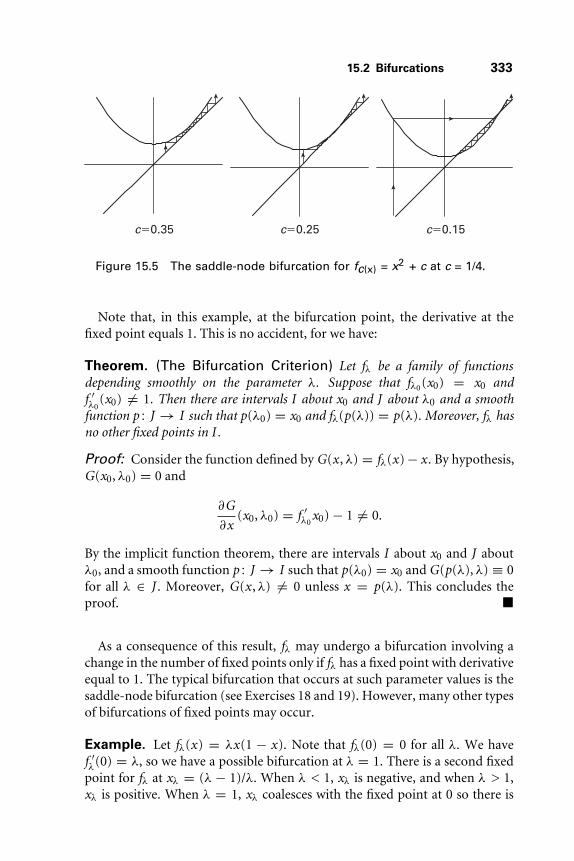
15.2 Bifurcations 333
c�0.35 c�0.25 c�0.15
Figure 15.5 The saddle-node bifurcation for fc(x) = x2 + c at c = 1/4.
Note that, in this example, at the bifurcation point, the derivative at thefixed point equals 1. This is no accident, for we have:
Theorem. (The Bifurcation Criterion) Let fλ be a family of functionsdepending smoothly on the parameter λ. Suppose that fλ0(x0) = x0 andf ′λ0
(x0) �= 1. Then there are intervals I about x0 and J about λ0 and a smoothfunction p : J → I such that p(λ0) = x0 and fλ(p(λ)) = p(λ). Moreover, fλ hasno other fixed points in I .
Proof: Consider the function defined by G(x , λ) = fλ(x) − x . By hypothesis,G(x0, λ0) = 0 and
∂G
∂x(x0, λ0) = f ′
λ0x0) − 1 �= 0.
By the implicit function theorem, there are intervals I about x0 and J aboutλ0, and a smooth function p : J → I such that p(λ0) = x0 and G(p(λ), λ) ≡ 0for all λ ∈ J . Moreover, G(x , λ) �= 0 unless x = p(λ). This concludes theproof. �
As a consequence of this result, fλ may undergo a bifurcation involving achange in the number of fixed points only if fλ has a fixed point with derivativeequal to 1. The typical bifurcation that occurs at such parameter values is thesaddle-node bifurcation (see Exercises 18 and 19). However, many other typesof bifurcations of fixed points may occur.
Example. Let fλ(x) = λx(1 − x). Note that fλ(0) = 0 for all λ. We havef ′λ(0) = λ, so we have a possible bifurcation at λ = 1. There is a second fixedpoint for fλ at xλ = (λ − 1)/λ. When λ < 1, xλ is negative, and when λ > 1,xλ is positive. When λ = 1, xλ coalesces with the fixed point at 0 so there is

334 Chapter 15 Discrete Dynamical Systems
a single fixed point for f1. A computation shows that 0 is repelling and xλ isattracting if λ > 1 (and λ < 3), while the reverse is true if λ < 1. For thisreason, this type of bifurcation is known as an exchange bifurcation. �
Example. Consider the family of functions fμ(x) = μx + x3. When μ = 1we have f1(0) = 0 and f ′
1 (0) = 1 so we have the possibility for a bifurcation.The fixed points are 0 and ±√
1 − μ, so we have three fixed points when μ < 1but only one fixed point when μ ≥ 1, so a bifurcation does indeed occur as μ
passes through 1. �
The only other possible bifurcation value for a one-dimensional discretesystem occurs when the derivative at the fixed (or periodic) point is equal to−1, since at these values the fixed point may change from a sink to a sourceor from a source to a sink. At all other values of the derivative, the fixed pointsimply remains a sink or source and there are no other periodic orbits nearby.Certain portions of a periodic orbit may come close to a source, but the entireorbit cannot lie close by (see Exercise 7). In the case of derivative −1 at thefixed point, the typical bifurcation is a period doubling bifurcation.
Example. As a simple example of this type of bifurcation, consider the familyfλ(x) = λx near λ0 = −1. There is a fixed point at 0 for all λ. When −1 <λ < 1, 0 is an attracting fixed point and all orbits tend to 0. When |λ| > 1, 0is repelling and all nonzero orbits tend to ±∞. When λ = −1, 0 is a neutralfixed point and all nonzero points lie on 2-cycles. As λ passes through −1,the type of the fixed point changes from attracting to repelling; meanwhile, afamily of 2-cycles appears. �
Generally, when a period doubling bifurcation occurs, the 2-cycles do notall exist for a single parameter value. A more typical example of this bifurcationis provided next.
Example. Again consider fc (x) = x2 + c , this time with c near c = −3/4.There is a fixed point at
p− = 1
2−
√1 − 4c
2.
We have seen that f ′−3/4(p−) = −1 and that p− is attracting when c is slightlylarger than −3/4 and repelling when c is less than −3/4. Graphical iterationshows that more happens as c descends through −3/4: We see the birth ofan (attracting) 2-cycle as well. This is the period doubling bifurcation. SeeFigure 15.6. Indeed, one can easily solve for the period two points and checkthat they are attracting (for −5/4 < c < −3/4; see Exercise 8). �

15.3 The Discrete Logistic Model 335
c = −0.65 c = −0.75 c = −0.85
Figure 15.6 The period doubling bifurcation for fc(x) = x2 + c at c = −3/4.The fixed point is attracting for c ≥ −0.75 and repelling for c < −0.75.
15.3 The Discrete Logistic Model
In Chapter 1 we introduced one of the simplest nonlinear first-orderdifferential equations, the logistic model for population growth
x ′ = ax(1 − x).
In this model we took into account the fact that there is a carrying capacityfor a typical population, and we saw that the resulting solutions behaved quitesimply: All nonzero solutions tended to the “ideal” population. Now some-thing about this model may have bothered you way back then: Populationsgenerally are not continuous functions of time! A more natural type of modelwould measure populations at specific times, say, every year or every gen-eration. Here we introduce just such a model, the discrete logistic model forpopulation growth.
Suppose we consider a population whose members are counted each year(or at other specified times). Let xn denote the population at the end of yearn. If we assume that no overcrowding can occur, then one such populationmodel is the exponential growth model where we assume that
xn+1 = kxn
for some constant k > 0. That is, the next year’s population is directlyproportional to this year’s. Thus we have
x1 = kx0
x2 = kx1 = k2x0
x3 = kx2 = k3x0
...

336 Chapter 15 Discrete Dynamical Systems
Clearly, xn = knx0 so we conclude that the population explodes if k > 1,becomes extinct if 0 ≤ k < 1, or remains constant if k = 1.
This is an example of a first-order difference equation. This is an equationthat determines xn based on the value of xn−1. A second-order differenceequation would give xn based on xn−1 and xn−2. From our point of view, thesuccessive populations are given by simply iterating the function fk(x) = kxwith the seed x0.
A more realistic assumption about population growth is that there is amaximal population M such that, if the population exceeds this amount, thenall resources are used up and the entire population dies out in the next year.
One such model that reflects these assumptions is the discrete logisticpopulation model . Here we assume that the populations obey the rule
xn+1 = kxn
(1 − xn
M
)where k and M are positive parameters. Note that, if xn ≥ M , then xn+1 ≤ 0,so the population does indeed die out in the ensuing year.
Rather than deal with actual population numbers, we will instead let xn
denote the fraction of the maximal population, so that 0 ≤ xn ≤ 1. Thelogistic difference equation then becomes
xn+1 = λxn (1 − xn)
where λ > 0 is a parameter. We may therefore predict the fate of the initialpopulation x0 by simply iterating the quadratic function fλ(x) = λx(1 − x)(also called the logistic map). Sounds easy, right? Well, suffice it to say thatthis simple quadratic iteration was only completely understood in the late1990s, thanks to the work of hundreds of mathematicians. We will see whythe discrete logistic model is so much more complicated than its cousin, thelogistic differential equation, in a moment, but first let’s do some simple cases.
We consider only the logistic map on the unit interval I . We have fλ(0) = 0,so 0 is a fixed point. The fixed point is attracting in I for 0 < λ ≤ 1, andrepelling thereafter. The point 1 is eventually fixed, since fλ(1) = 0. Thereis a second fixed point xλ = (λ − 1)/λ in I for λ > 1. The fixed point xλ isattracting for 1 < λ ≤ 3 and repelling for λ > 3. At λ = 3 a period doublingbifurcation occurs (see Exercise 4). For λ-values between 3 and approximately3. 4, the only periodic points present are the two fixed points and the 2-cycle.
When λ = 4, the situation is much more complicated. Note that f ′λ(1/2) = 0
and that 1/2 is the only critical point for fλ for each λ. When λ = 4, we havef4(1/2) = 1, so f 2
4 (1/2) = 0. Therefore f4 maps each of the half-intervals[0, 1/2] and [1/2, 1] onto the entire interval I . Consequently, there exist pointsy0 ∈ [0, 1/2] and y1 ∈ [1/2, 1] such that f4(yj) = 1/2 and hence f 2
4 (yj) = 1.

15.4 Chaos 337
1/2 1/2 1/2y0 y1 y0 y1
Figure 15.7 The graphs of the logistic function fλ(x) − λ x(1 − x) as well asf 2λ and f 3
λ over the interval I.
Therefore we have
f 24 [0, y0] = f 2
4 [y0, 1/2] = I
and
f 24 [1/2, y1] = f 2
4 [y1, 1] = I .
Since the function f 24 is a quartic, it follows that the graph of f 2
4 is as depictedin Figure 15.7. Continuing in this fashion, we find 23 subintervals of I that aremapped onto I by f 3
4 , 24 subintervals mapped onto I by f 44 , and so forth. We
therefore see that f4 has two fixed points in I ; f 24 has four fixed points in I ; f 3
4has 23 fixed points in I ; and, inductively, f n
4 has 2n fixed points in I . The fixedpoints for f4 occur at 0 and 3/4. The four fixed points for f 2
4 include these twofixed points plus a pair of periodic points of period 2. Of the eight fixed pointsfor f 3
4 , two must be the fixed points and the other six must lie on a pair of3-cycles. Among the 16 fixed points for f 4
4 are two fixed points, two periodicpoints of period 2, and twelve periodic points of period 4. Clearly, a lot haschanged as λ varies from 3. 4 to 4.
On the other hand, if we choose a random seed in the interval I and plotthe orbit of this seed under iteration of f4 using graphical iteration, we rarelysee any of these cycles. In Figure 15.8 we have plotted the orbit of 0. 123 underiteration of f4 using 200 and 500 iterations. Presumably, there is something“chaotic” going on.
15.4 Chaos
In this section we introduce several quintessential examples of chaotic one-dimensional discrete dynamical systems. Recall that a subset U ⊂ W is said

338 Chapter 15 Discrete Dynamical Systems
(a) (b)
Figure 15.8 The orbit of the seed 0.123 under f4 using (a) 200iterations and (b) 500 iterations.
to be dense in W if there are points in U arbitrarily close to any point in thelarger set W . As in the Lorenz model, we say that a map f , which takes aninterval I = [α, β] to itself, is chaotic if
1. Periodic points of f are dense in I ;2. f is transitive on I ; that is, given any two subintervals U1 and U2 in I ,
there is a point x0 ∈ U1 and an n > 0 such that f n(x0) ∈ U2;3. f has sensitive dependence in I ; that is, there is a sensitivity constant β
such that, for any x0 ∈ I and any open interval U about x0, there is someseed y0 ∈ U and n > 0 such that
|f n(x0) − f n(y0)| > β.
It is known that the transitivity condition is equivalent to the existence ofan orbit that is dense in I . Clearly, a dense orbit implies transitivity, for suchan orbit repeatedly visits any open subinterval in I . The other direction relieson the Baire category theorem from analysis, so we will not prove this here.
Curiously, for maps of an interval, condition 3 in the definition of chaos isredundant [8]. This is somewhat surprising, since the first two conditions inthe definition are topological in nature, while the third is a metric property (itdepends on the notion of distance).
We now discuss several classical examples of chaotic one-dimensional maps.
Example. (The Doubling Map) Define the discontinuous functionD : [0, 1) → [0, 1) by D(x) = 2x mod 1. That is,
D(x) ={
2x if 0 ≤ x < 1/22x − 1 if 1/2 ≤ x < 1

15.4 Chaos 339
Figure 15.9 The graph of the doubling map D and its higher iterates D2
and D3 on [0, 1).
An easy computation shows that Dn(x) = 2nx mod 1, so that the graph ofDn consists of 2n straight lines with slope 2n , each extending over the entireinterval [0, 1). See Figure 15.9.
To see that the doubling function is chaotic on [0, 1), note that Dn maps anyinterval of the form [k/2n , (k + 1)/2n) for k = 0, 1, . . . 2n − 2 onto the interval[0, 1). Hence the graph of Dn crosses the diagonal y = x at some point in thisinterval, and so there is a periodic point in any such interval. Since the lengthsof these intervals are 1/2n , it follows that periodic points are dense in [0, 1).Transitivity also follows, since, given any open interval J , we may always findan interval of the form [k/2n , (k +1)/2n) inside J for sufficiently large n. HenceDn maps J onto all of [0, 1). This also proves sensitivity, where we choose thesensitivity constant 1/2.
We remark that it is possible to write down all of the periodic points forD explicitly (see Exercise 5a). It is also interesting to note that, if you usea computer to iterate the doubling function, then it appears that all orbitsare eventually fixed at 0, which, of course, is false! See Exercise 5c for anexplanation of this phenomenon. �
Example. (The Tent Map) Now consider a continuous cousin of thedoubling map given by
T (x) ={
2x if 0 ≤ x < 1/2−2x + 2 if 1/2 ≤ x ≤ 1.
T is called the tent map. See Figure 15.10. The fact that T is chaotic on [0, 1]follows exactly as in the case of the doubling function, using the graphs of T n
(see Exercise 15).Looking at the graphs of the tent function T and the logistic function f4(x) =
4x(1 − x) that we discussed in Section 15.3, it appears that they should sharemany of the same properties under iteration. Indeed, this is the case. Tounderstand this, we need to reintroduce the notion of conjugacy, this time fordiscrete systems.

340 Chapter 15 Discrete Dynamical Systems
Figure 15.10 The graph of the tent map T and its higher iterates T 2 andT 3 on [0, 1].
Suppose I and J are intervals and f : I → I and g : J → J . We say that fand g are conjugate if there is a homeomorphism h : I → J such that h satisfiesthe conjugacy equation h ◦ f = g ◦ h. Just as in the case of flows, a conjugacytakes orbits of f to orbits of g . This follows since we have h(f n(x)) = g n(h(x))for all x ∈ I , so h takes the nth point on the orbit of x under f to thenth point on the orbit of h(x) under g . Similarly, h−1 takes orbits of g toorbits of f . �
Example. Consider the logistic function f4 : [0, 1] → [0, 1] and the quadraticfunction g : [−2, 2] → [−2, 2] given by g (x) = x2 − 2. Let h(x) = −4x + 2and note that h takes [0, 1] to [−2, 2]. Moreover, we have h(4x(1 −x)) = (h(x))2 − 2, so h satisfies the conjugacy equation and f4 and g areconjugate. �
From the point of view of chaotic systems, conjugacies are important sincethey map one chaotic system to another.
Proposition. Suppose f : I → I and g : J → J are conjugate via h, whereboth I and J are closed intervals in R of finite length. If f is chaotic on I , then gis chaotic on J .
Proof: Let U be an open subinterval of J and consider h−1(U ) ⊂ I . Sinceperiodic points of f are dense in I , there is a periodic point x ∈ h−1(U ) for f .Say x has period n. Then
g n(h(x)) = h(f n(x)) = h(x)
by the conjugacy equation. This gives a periodic point h(x) for g in U andshows that periodic points of g are dense in J .
If U and V are open subintervals of J , then h−1(U ) and h−1(V ) are openintervals in I . By transitivity of f , there exists x1 ∈ h−1(U ) such that

15.4 Chaos 341
f m(x1) ∈ h−1(V ) for some m. But then h(x1) ∈ U and we have gm(h(x1)) =h(f m(x1)) ∈ V , so g is transitive also.
For sensitivity, suppose that f has sensitivity constant β. Let I = [α0, α1].We may assume that β < α1 − α0. For any x ∈ [α0, α1 − β], consider thefunction |h(x + β) − h(x)|. This is a continuous function on [α0, α1 − β]that is positive. Hence it has a minimum value β ′. It follows that h takesintervals of length β in I to intervals of length at least β ′ in J . Then itis easy to check that β ′ is a sensitivity constant for g . This completes theproof. �
It is not always possible to find conjugacies between functions with equiva-lent dynamics. However, we can relax the requirement that the conjugacy beone to one and still salvage the preceding proposition. A continuous function hthat is at most n to one and that satisfies the conjugacy equation f ◦h = h◦g iscalled a semiconjugacy between g and f . It is easy to check that a semiconjugacyalso preserves chaotic behavior on intervals of finite length (see Exercise 12).A semiconjugacy need not preserve the minimal periods of cycles, but it doesmap cycles to cycles.
Example. The tent function T and the logistic function f4 are semiconjugateon the unit interval. To see this, let
h(x) = 1
2(1 − cos 2πx) .
Then h maps the interval [0, 1] in two-to-one fashion over itself, except at 1/2,which is the only point mapped to 1. Then we compute
h(T (x)) = 1
2(1 − cos 4πx)
= 1
2− 1
2
(2 cos2 2πx − 1
)= 1 − cos2 2πx
= 4
(1
2− 1
2cos 2πx
)(1
2+ 1
2cos 2πx
)= f4(h(x)).
Thus h is a semiconjugacy between T and f4. As a remark, recall that we mayfind arbitrarily small subintervals mapped onto all of [0, 1]by T . Hence f4 mapsthe images of these intervals under h onto all of [0, 1]. Since h is continuous,the images of these intervals may be chosen arbitrarily small. Hence we may

342 Chapter 15 Discrete Dynamical Systems
choose 1/2 as a sensitivity constant for f4 as well. We have proven the followingproposition: �
Proposition. The logistic function f4(x) = 4x(1 − x) is chaotic on the unitinterval. �
15.5 Symbolic Dynamics
We turn now to one of the most useful tools for analyzing chaotic systems,symbolic dynamics. We give just one example of how to use symbolic dynamicshere; several more are included in the next chapter.
Consider the logistic map fλ(x) = λx(1 − x) where λ > 4. Graphical iter-ation seems to imply that almost all orbits tend to −∞. See Figure 15.11.Of course, this is not true, because we have fixed points and other peri-odic points for this function. In fact, there is an unexpectedly “large” setcalled a Cantor set that is filled with chaotic behavior for this function, as weshall see.
Unlike the case λ ≤ 4, the interval I = [0, 1] is no longer invariant whenλ > 4: Certain orbits escape from I and then tend to −∞. Our goal is tounderstand the behavior of the nonescaping orbits. Let � denote the set ofpoints in I whose orbits never leave I . As shown in Figure 15.12a, there isan open interval A0 on which fλ > 1. Hence f 2
λ (x) < 0 for any x ∈ A0 and,as a consequence, the orbits of all points in A0 tend to −∞. Note that anyorbit that leaves I must first enter A0 before departing toward −∞. Also, the
1
Figure 15.11 Typicalorbits for the logisticfunction fλ with λ > 4seem to tend to −∞ afterwandering around the unitinterval for a while.

15.5 Symbolic Dynamics 343
A1 A1A0(a)
I0 I1A0(b)
Figure 15.12 (a) The exit set in I consists of a collectionof disjoint open intervals. (b) The intervals I0 and I1 lie tothe left and right of A0 .
orbits of the endpoints of A0 are eventually fixed at 0, so these endpoints arecontained in �. Now let A1 denote the preimage of A0 in I : A1 consists oftwo open intervals in I , one on each side of A0. All points in A1 are mappedinto A0 by fλ, and hence their orbits also tend to −∞. Again, the endpointsof A1 are eventual fixed points. Continuing, we see that each of the two openintervals in A1 has as a preimage a pair of disjoint intervals, so there are fouropen intervals that consist of points whose first iteration lies in A1, the secondin A0, and so, again, all of these points have orbits that tend to −∞. Call thesefour intervals A2. In general, let An denote the set of points in I whose nthiterate lies in A0. An consists of set 2n disjoint open intervals in I . Any pointwhose orbit leaves I must lie in one of the An . Hence we see that
� = I −∞⋃
n=0
An .
To understand the dynamics of fλ on I , we introduce symbolic dynamics.Toward that end, let I0 and I1 denote the left and right closed interval respec-tively in I − A0. See Figure 15.12b. Given x0 ∈ �, the entire orbit of x0 liesin I0 ∪ I1. Hence we may associate an infinite sequence S(x0) = (s0s1s2 . . .)consisting of 0’s and 1’s to the point x0 via the rule
sj = k if and only if fjλ (x0) ∈ Ik .
That is, we simply watch how fjλ (x0) bounces around I0 and I1, assigning a 0
or 1 at the jth stage depending on which interval fjλ (x0) lies in. The sequence
S(x0) is called the itinerary of x0.

344 Chapter 15 Discrete Dynamical Systems
Example. The fixed point 0 has itinerary S(0) = (000 . . .). The fixed point xλ
in I1 has itinerary S(xλ) = (111 . . .). The point x0 = 1 is eventually fixed andhas itinerary S(1) = (1000 . . .). A 2-cycle that hops back and forth between I0and I1 has itinerary (01 . . .) or (10 . . .) where 01 denotes the infinitely repeatingsequence consisting of repeated blocks 01.
Let � denote the set of all possible sequences of 0’s and 1’s. A “point” inthe space � is therefore an infinite sequence of the form s = (s0s1s2 . . .). Tovisualize �, we need to tell how far apart different points in � are. To do this,let s = (s0s1s2 . . .) and t = (t0t1t2 . . .) be points in �. A distance function ormetric on � is a function d = d(s, t ) that satisfies
1. d(s, t ) ≥ 0 and d(s, t ) = 0 if and only if s = t ;2. d(s, t ) = d(t , s);3. the triangle inequality: d(s, u) ≤ d(s, t ) + d(t , u).
Since � is not naturally a subset of a Euclidean space, we do not have aEuclidean distance to use on �. Hence we must concoct one of our own. Hereis the distance function we choose:
d(s, t ) =∞∑
i=0
|si − ti |2i
.
Note that this infinite series converges: The numerators in this series are alwayseither 0 or 1, so this series converges by comparison to the geometric series:
d(s, t ) ≤∞∑
i=0
1
2i= 1
1 − 1/2= 2.
It is straightforward to check that this choice of d satisfies the three require-ments to be a distance function (see Exercise 13). While this distance functionmay look a little complicated at first, it is often easy to compute. �
Example.
(1) d((0), (1)
) =∞∑
i=0
|0 − 1|2i
=∞∑
i=0
1
2i= 2
(2) d((01), (10)
) =∞∑
i=0
1
2i= 2
(3) d((01), (1)
) =∞∑
i=0
1
4i= 1
1 − 1/4= 4
3.
�

15.5 Symbolic Dynamics 345
The importance of having a distance function on � is that we now knowwhen points are close together or far apart. In particular, we have
Proposition. Suppose s = (s0s1s2 . . .) and t = (t0t1t2 . . .) ∈ �.
1. If sj = tj for j = 0, . . . , n, then d(s, t ) ≤ 1/2n;2. Conversely, if d(s, t ) < 1/2n, then sj = tj for j = 0, . . . , n.
Proof: In case (1), we have
d(s, t ) =n∑
i=0
|si − si |2i
+∞∑
i=n+1
|si − ti |2i
≤ 0 + 1
2n+1
∞∑i=0
1
2i
= 1
2n.
If, on the other hand, d(s, t ) < 1/2n , then we must have sj = tj for any j ≤ n,because otherwise d(s, t ) ≥ |sj − tj |/2j = 1/2j ≥ 1/2n . �
Now that we have a notion of closeness in �, we are ready to prove the maintheorem of this chapter:
Theorem. The itinerary function S : � → � is a homeomorphism providedλ > 4.
Proof: Actually, we will only prove this for the case in which λ is sufficientlylarge that |f ′
λ(x)| > K > 1 for some K and for all x ∈ I0 ∪ I1. The reader may
check that λ > 2 + √5 suffices for this. For the more complicated proof in the
case where 4 < λ ≤ 2 + √5, see [25].
We first show that S is one to one. Let x , y ∈ � and suppose S(x) = S(y).Then, for each n, f n
λ (x) and f nλ (y) lie on the same side of 1/2. This implies that
fλ is monotone on the interval between f nλ (x) and f n
λ (y). Consequently, allpoints in this interval remain in I0 ∪ I1 when we apply fλ. Now |f ′
λ| > K > 1 atall points in this interval, so, as in Section 15.1, each iteration of fλ expands thisinterval by a factor of K . Hence the distance between f n
λ (x) and f nλ (y) grows
without bound, so these two points must eventually lie on opposite sides ofA0. This contradicts the fact that they have the same itinerary.
To see that S is onto, we first introduce the following notation. Let J ⊂ I bea closed interval. Let
f −nλ (J ) = {x ∈ I | f n
λ (x) ∈ J },

346 Chapter 15 Discrete Dynamical Systems
so that f −nλ (J ) is the preimage of J under f n
λ . A glance at the graph of fλ whenλ > 4 shows that, if J ⊂ I is a closed interval, then f −1
λ (J ) consists of twoclosed subintervals, one in I0 and one in I1.
Now let s = (s0s1s2 . . .). We must produce x ∈ � with S(x) = s. To thatend we define
Is0s1...sn = {x ∈ I | x ∈ Is0 , fλ(x) ∈ Is1 , . . . , fnλ (x) ∈ Isn }
= Is0 ∩ f −1λ (Is1) ∩ . . . ∩ f −n
λ (Isn ).
We claim that the Is0...sn form a nested sequence of nonempty closedintervals. Note that
Is0s1...sn = Is0 ∩ f −1λ (Is1...sn ).
By induction, we may assume that Is1...sn is a nonempty subinterval, so that, bythe observation above, f −1
λ (Is1...sn ) consists of two closed intervals, one in I0and one in I1. Hence Is0 ∩ f −1
λ (Is1...sn ) is a single closed interval. These intervalsare nested because
Is0...sn = Is0...sn−1 ∩ f −nλ (Isn ) ⊂ Is0...sn−1 .
Therefore we conclude that
∞⋂n≥0
Is0s1...sn
is nonempty. Note that if x ∈ ∩n≥0Is0s1...sn , then x ∈ Is0 , fλ(x) ∈ Is1 , etc. HenceS(x) = (s0s1 . . .). This proves that S is onto.
Observe that ∩n≥0Is0s1...sn consists of a unique point. This follows immedi-ately from the fact that S is one to one. In particular, we have that the diameterof Is0s1...sn tends to 0 as n → ∞.
To prove continuity of S, we choose x ∈ � and suppose that S(x) =(s0s1s2 . . .). Let ε > 0. Pick n so that 1/2n < ε. Consider the closed subin-tervals It0t1...tn defined above for all possible combinations t0t1 . . . tn . Thesesubintervals are all disjoint, and � is contained in their union. There are2n+1 such subintervals, and Is0s1...sn is one of them. Hence we may choose δ
such that |x − y| < δ and y ∈ � implies that y ∈ Is0s1...sn . Therefore, S(y)agrees with S(x) in the first n + 1 terms. So, by the previous proposition,we have
d(S(x), S(y)) ≤ 1
2n< ε.

15.6 The Shift Map 347
This proves the continuity of S. It is easy to check that S−1 is also continuous.Thus, S is a homeomorphism. �
15.6 The Shift Map
We now construct a map on σ : � → � with the following properties:
1. σ is chaotic;2. σ is conjugate to fλ on �;3. σ is completely understandable from a dynamical systems point of view.
The meaning of this last item will become clear as we proceed.We define the shift map σ : � → � by
σ (s0s1s2 . . .) = (s1s2s3 . . .).
That is, the shift map simply drops the first digit in each sequence in �. Notethat σ is a two-to-one map onto �. This follows since, if (s0s1s2 . . .) ∈ �, thenwe have
σ (0s0s1s2 . . .) = σ (1s0s1s2 . . .) = (s0s1s2 . . .).
Proposition. The shift map σ : � → � is continuous.
Proof: Let s = (s0s1s2 . . .) ∈ �, and let ε > 0. Choose n so that 1/2n < ε. Letδ = 1/2n+1. Suppose that d(s, t ) < δ, where t = (t0t1t2 . . .). Then we havesi = ti for i = 0, . . . , n + 1.
Now σ (t ) = (s1s2 . . . sntn+1tn+2 . . .) so that d(σ (s), σ (t )) ≤ 1/2n < ε. Thisproves that σ is continuous. �
Note that we can easily write down all of the periodic points of any periodfor the shift map. Indeed, the fixed points are (0) and (1). The 2 cycles are (01)and (10). In general, the periodic points of period n are given by repeatingsequences that consist of repeated blocks of length n: (s0 . . . sn−1). Note howmuch nicer σ is compared to fλ: Just try to write down explicitly all of theperiodic points of period n for fλ someday! They are there and we knowroughly where they are, because we have:
Theorem. The itinerary function S : � → � provides a conjugacy between fλand the shift map σ .
Proof: In the previous section we showed that S is a homeomorphism. So itsuffices to show that S ◦ fλ = σ ◦ S. To that end, let x0 ∈ � and suppose

348 Chapter 15 Discrete Dynamical Systems
that S(x0) = (s0s1s2 . . .). Then we have x0 ∈ Is0 , fλ(x0) ∈ Is1 , f 2λ (x0) ∈ Is2 ,
and so forth. But then the fact that fλ(x0) ∈ Is1 , f 2λ (x0) ∈ Is2 , etc., says that
S(fλ(x0)) = (s1s2s3 . . .), so S(fλ(x0)) = σ (S(x0)), which is what we wanted toprove. �
Now, not only can we write down all periodic points for σ , but we can infact write down explicitly a point in � whose orbit is dense. Here is such apoint:
s∗ = ( 0 1︸︷︷︸1 blocks
| 00 01 10 11︸ ︷︷ ︸2 blocks
| 000 001 · · ·︸ ︷︷ ︸3 blocks
| · · ·︸︷︷︸4 blocks
).
The sequence s∗ is constructed by successively listing all possible blocks of 0’sand 1’s of length 1, length 2, length 3, and so forth. Clearly, some iterate ofσ applied to s∗ yields a sequence that agrees with any given sequence in anarbitrarily large number of initial places. That is, given t = (t0t1t2 . . .) ∈ �,we may find k so that the sequence σ k(s∗) begins
(t0 . . . tn sn+1 sn+2 . . .)
so that
d(σ k(s∗), t ) ≤ 1/2n .
Hence the orbit of s∗ comes arbitrarily close to every point in �. This provesthat the orbit of s∗ under σ is dense in � and so σ is transitive. Note thatwe may construct a multitude of other points with dense orbits in � by justrearranging the blocks in the sequence s∗. Again, think about how difficult itwould be to identify a seed whose orbit under a quadratic function like f4 isdense in [0, 1]. This is what we meant when we said earlier that the dynamicsof σ are “completely understandable.”
The shift map also has sensitive dependence. Indeed, we may choose thesensitivity constant to be 2, which is the largest possible distance between twopoints in �. The reason for this is, if s = (s0s1s2 . . .) ∈ � and sj denotes “notsj” (that is, if sj = 0, then sj = 1, or if sj = 1 then sj = 0), then the points ′ = (s0s1 . . . sn sn+1sn+2 . . .) satisfies:
1. d(s, s ′) = 1/2n , but2. d(σ n(s), σ n(s ′)) = 2.
As a consequence, we have proved the following:
Theorem. The shift map σ is chaotic on �, and so by the conjugacy in theprevious theorem, the logistic map fλ is chaotic on � when λ > 4. �

15.7 The Cantor Middle-Thirds Set 349
Thus symbolic dynamics provides us with a computable model for thedynamics of fλ on the set �, despite the fact that fλ is chaotic on �.
15.7 The Cantor Middle-Thirds Set
We mentioned earlier that � was an example of a Cantor set. Here we describethe simplest example of such a set, the Cantor middle-thirds set C. As we shallsee, this set has some unexpectedly interesting properties.
To define C , we begin with the closed unit interval I = [0, 1]. The ruleis, each time we see a closed interval, we remove its open middle third.Hence, at the first stage, we remove (1/3, 2/3), leaving us with two closedintervals, [0, 1/3] and [2/3, 1]. We now repeat this step by removing themiddle thirds of these two intervals. We are left with four closed intervals[0, 1/9], [2/9, 1/3], [2/3, 7/9], and [8/9, 1]. Removing the open middle thirds ofthese intervals leaves us with 23 closed intervals, each of length 1/33. Continu-ing in this fashion, at the nth stage we are left with 2n closed intervals each oflength 1/3n . The Cantor middle-thirds set C is what is left when we take thisprocess to the limit as n → ∞. Note how similar this construction is to thatof � in Section 15.5. In fact, it can be proved that � is homeomorphic to C(see Exercises 16 and 17).
What points in I are left in C after removing all of these open intervals?Certainly 0 and 1 remain in C , as do the endpoints 1/3 and 2/3 of the firstremoved interval. Indeed, each endpoint of a removed open interval liesin C because such a point never lies in an open middle-third subinterval.At first glance, it appears that these are the only points in the Cantor set,but in fact, that is far from the truth. Indeed, most points in C are notendpoints!
To see this, we attach an address to each point in C . The address will bean infinite string of L’s or R’s determined as follows. At each stage of theconstruction, our point lies in one of two small closed intervals, one to theleft of the removed open interval or one to its right. So at the nth stage wemay assign an L or R to the point depending on its location left or right ofthe interval removed at that stage. For example, we associate LLL . . . to 0and RRR . . . to 1. The endpoints 1/3 and 2/3 have addresses LRRR . . . andRLLL . . . , respectively. At the next stage, 1/9 has address LLRRR . . . since 1/9lies in [0, 1/3] and [0, 1/9] at the first two stages, but then always lies in theright-hand interval. Similarly, 2/9 has address LRLLL . . . , while 7/9 and 8/9have addresses RLRRR . . . and RRLLL . . . .
Notice what happens at each endpoint of C . As the above examples indicate,the address of an endpoint always ends in an infinite string of all L’s or all R’s.But there are plenty of other possible addresses for points in C . For example,

350 Chapter 15 Discrete Dynamical Systems
there is a point with address LRLRLR . . . . This point lies in
[0, 1/3] ∩ [2/9, 1/3] ∩ [2/9, 7/27] ∩ [20/81, 7/27] . . . .
Note that this point lies in the nested intersection of closed intervals of length1/3n for each n, and it is the unique such point that does so. This shows thatmost points in C are not endpoints, for the typical address will not end in allL’s or all R’s.
We can actually say quite a bit more: The Cantor middle-thirds set containsuncountably many points. Recall that an infinite set is countable if it can beput in one-to-one correspondence with the natural numbers; otherwise, theset is uncountable.
Proposition. The Cantor middle-thirds set is uncountable.
Proof: Suppose that C is countable. This means that we can pair each pointin C with a natural number in some fashion, say as
1 : LLLLL . . .
2 : RRRR . . .
3 : LRLR . . .
4 : RLRL . . .
5 : LRRLRR . . .
and so forth. But now consider the address whose first entry is the oppositeof the first entry of sequence 1, whose second entry is the opposite of thesecond entry of sequence 2; and so forth. This is a new sequence of L’s and R’s(which, in the example above, begins with RLRRL . . .). Thus we have createda sequence of L’s and R’s that disagrees in the nth spot with the nth sequenceon our list. Hence this sequence is not on our list and so we have failed in ourconstruction of a one-to-one correspondence with the natural numbers. Thiscontradiction establishes the result. �
We can actually determine the points in the Cantor middle-thirds set in amore familiar way. To do this we change the address of a point in C from asequence of L’s and R’s to a sequence of 0’s and 2’s; that is, we replace eachL with a 0 and each R with a 2. To determine the numerical value of a pointx ∈ C we approach x from below by starting at 0 and moving sn/3n units to theright for each n, where sn = 0 or 2 depending on the nth digit in the addressfor n = 1, 2, 3 . . . .

15.7 The Cantor Middle-Thirds Set 351
For example, 1 has address RRR . . . or 222 . . . , so 1 is given by
2
3+ 2
32+ 2
33+ · · · = 2
3
∞∑n=0
1
3n= 2
3
(1
1 − 1/3
)= 1.
Similarly, 1/3 has address LRRR . . . or 0222 . . . , which yields
0
3+ 2
32+ 2
33+ · · · = 2
9
∞∑n=0
1
3n= 2
9· 3
2= 1
3.
Finally, the point with address LRLRLR . . . or 020202 . . . is
0
3+ 2
32+ 0
33+ 2
34+ · · · = 2
9
∞∑n=0
1
9n= 2
9
(1
1 − 1/9
)= 1
4.
Note that this is one of the non-endpoints in C referred to earlier.The astute reader will recognize that the address of a point x in C with 0’s
and 2’s gives the ternary expansion of x . A point x ∈ I has ternary expansiona1a2a3 . . . if
x =∞∑
i=1
ai
3i
where each ai is either 0, 1, or 2. Thus we see that points in the Cantor middle-thirds set have ternary expansions that may be written with no 1’s among thedigits.
We should be a little careful here. The ternary expansion of 1/3 is 1000 . . . .But 1/3 also has ternary expansion 0222 . . . as we saw above. So 1/3 may bewritten in ternary form in a way that contains no 1’s. In fact, every endpoint inC has a similar pair of ternary representations, one of which contains no 1’s.
We have shown that C contains uncountably many points, but we can sayeven more:
Proposition. The Cantor middle-thirds set contains as many points as theinterval [0, 1].Proof: C consists of all points whose ternary expansion a0a1a2 . . . containsonly 0’s or 2’s. Take this expansion and change each 2 to a 1 and then thinkof this string as a binary expansion. We get every possible binary expansion inthis manner. We have therefore made a correspondence (at most two to one)between the points in C and the points in [0, 1], since every such point has abinary expansion. �

352 Chapter 15 Discrete Dynamical Systems
Finally, we note that
Proposition. The Cantor middle-thirds set has length 0.
Proof: We compute the “length” of C by adding up the lengths of the intervalsremoved at each stage to determine the length of the complement of C . Theseremoved intervals have successive lengths 1/3, 2/9, 4/27… and so the length ofI − C is
1
3+ 2
9+ 4
27+ · · · = 1
3
∞∑n=0
(2
3
)n
= 1.�
This fact may come as no surprise since C consists of a “scatter” of points.But now consider the Cantor middle-fifths set, obtained by removing the openmiddle-fifth of each closed interval in similar fashion to the construction ofC . The length of this set is nonzero, yet it is homeomorphic to C . TheseCantor sets have, as we said earlier, unexpectedly interesting properties! Andremember, the set � on which f4 is chaotic is just this kind of object.
15.8 Exploration: Cubic Chaos
In this exploration, you will investigate the behavior of the discrete dynamicalsystem given by the family of cubic functions fλ(x) = λx − x3. You shouldattempt to prove rigorously everything outlined below.
1. Describe the dynamics of this family of functions for all λ < −1.2. Describe the bifurcation that occurs at λ = −1. Hint: Note that fλ is an
odd function. In particular, what happens when the graph of fλ crossesthe line y = −x?
3. Describe the dynamics of fλ when −1 < λ < 1.4. Describe the bifurcation that occurs at λ = 1.5. Find a λ-value, λ∗, for which fλ∗ has a pair of invariant intervals [0, ±x∗]
on each of which the behavior of fλ mimics that of the logistic function4x(1 − x).
6. Describe the change in dynamics that occurs when λ increasesthrough λ∗.
7. Describe the dynamics of fλ when λ is very large. Describe the set ofpoints �λ whose orbits do not escape to ±∞ in this case.
8. Use symbolic dynamics to set up a sequence space and a correspondingshift map for λ large. Prove that fλ is chaotic on �λ.
9. Find the parameter value λ′ > λ∗ above, which the results of the previoustwo investigations hold true.
10. Describe the bifurcation that occurs as λ increases through λ′.

15.9 Exploration: The Orbit Diagram 353
15.9 Exploration: The Orbit Diagram
Unlike the previous exploration, this exploration is primarily experimental.It is designed to acquaint you with the rich dynamics of the logistic family asthe parameter increases from 0 to 4. Using a computer and whatever softwareseems appropriate, construct the orbit diagram for the logistic family fλ(x) =λx(1 − x) as follows: Choose N equally spaced λ-values λ1, λ2, . . . , λN in theinterval 0 ≤ λj ≤ 4. For example, let N = 800 and set λj = 0. 005j . For eachλj , compute the orbit of 0. 5 under fλj and plot this orbit as follows.
Let the horizontal axis be the λ-axis and let the vertical axis be the x-axis.Over each λj , plot the points (λj , f k
λj(0. 5)) for, say, 50 ≤ k ≤ 250. That is,
compute the first 250 points on the orbit of 0. 5 under fλj , but display only thelast 200 points on the vertical line over λ = λj . Effectively, you are displayingthe “fate” of the orbit of 0. 5 in this way.
You will need to magnify certain portions of this diagram; one such magni-fication is displayed in Figure 15.13, where we have displayed only that portionof the orbit diagram for λ in the interval 3 ≤ λ ≤ 4.
1. The region bounded by 0 ≤ λ < 3. 57 . . . is called the period 1 win-dow. Describe what you see as λ increases in this window. What type ofbifurcations occur?
2. Near the bifurcations in the previous question, you sometimes see a smearof points. What causes this?
3. Observe the period 3 window bounded approximately by 3. 828 . . . < λ <3. 857 . . . . Investigate the bifurcation that gives rise to this window as λ
increases.
3
x
4λ
3.57 3.83
Figure 15.13 The orbit diagram for the logistic family with3 ≤ λ ≤ 4.

354 Chapter 15 Discrete Dynamical Systems
4. There are many other period n windows (named for the least period ofthe cycle in that window). Discuss any pattern you can find in how thesewindows are arranged asλ increases. In particular, if you magnify portionsbetween the period 1 and period 3 windows, how are the larger windowsin each successive enlargement arranged?
5. You observe “darker” curves in this orbit diagram. What are these? Whydoes this happen?
E X E R C I S E S
1. Find all periodic points for each of the following maps and classify themas attracting, repelling, or neither.
(a) Q(x) = x − x2 (b) Q(x) = 2(x − x2)(c) C(x) = x3 − 1
9x (d) C(x) = x3 − x(e) S(x) = 1
2 sin(x) (f) S(x) = sin(x)(g) E(x) = ex−1 (h) E(x) = ex
(i) A(x) = arctan x (j) A(x) = −π4 arctan x
2. Discuss the bifurcations that occur in the following families of maps atthe indicated parameter value
(a) Sλ(x) = λ sin x , λ = 1
(b) Cμ(x) = x3 + μx , μ = −1 (Hint: Exploit the fact that Cμ is anodd function.)
(c) Gν(x) = x + sin x + ν, ν = 1
(d) Eλ(x) = λex , λ = 1/e
(e) Eλ(x) = λex , λ = −e
(f) Aλ(x) = λ arctan x , λ = 1
(g) Aλ(x) = λ arctan x , λ = −1
3. Consider the linear maps fk(x) = kx . Show that there are four open setsof parameters for which the behavior of orbits of fk is similar. Describewhat happens in the exceptional cases.
4. For the function fλ(x) = λx(1 − x) defined on R:
(a) Describe the bifurcations that occur at λ = −1 and λ = 3.
(b) Find all period 2 points.
(c) Describe the bifurcation that occurs at λ = −1. 75.
5. For the doubling map D on [0, 1):
(a) List all periodic points explicitly.

Exercises 355
(b) List all points whose orbits end up landing on 0 and are therebyeventually fixed.
(c) Let x ∈ [0, 1) and suppose that x is given in binary form as a0a1a2 . . .where each aj is either 0 or 1. First give a formula for the binaryrepresentation of D(x). Then explain why this causes orbits of Dgenerated by a computer to end up eventually fixed at 0.
6. Show that, if x0 lies on a cycle of period n, then
(f n)′(x0) =n−1∏i=0
f ′(xi).
Conclude that
(f n)′(x0) = (f n)′(xj)
for j = 1, . . . , n − 1.7. Prove that if fλ0 has a fixed point at x0 with |f ′
λ0(x0)| > 1, then there is an
interval I about x0 and an interval J about λ0 such that, if λ ∈ J , then fλhas a unique fixed source in I and no other orbits that lie entirely in I .
8. Verify that the family fc (x) = x2 + c undergoes a period doublingbifurcation at c = −3/4 by
(a) Computing explicitly the period two orbit.(b) Showing that this orbit is attracting for −5/4 < c < −3/4.
9. Show that the family fc (x) = x2 + c undergoes a second period doublingbifurcation at c = −5/4 by using the graphs of f 2
c and f 4c .
10. Find an example of a bifurcation in which more than three fixed pointsare born.
11. Prove that f3(x) = 3x(1 − x) on I is conjugate to f (x) = x2 − 3/4 on acertain interval in R. Determine this interval.
12. Suppose f , g : [0, 1] → [0, 1] and that there is a semiconjugacy from f tog . Suppose that f is chaotic. Prove that g is also chaotic on [0, 1].
13. Prove that the function d(s, t ) on � satisfies the three properties requiredfor d to be a distance function or metric.
14. Identify the points in the Cantor middle-thirds set C whoseaddresses are
(a) LLRLLRLLR . . .(b) LRRLLRRLLRRL . . .
15. Consider the tent map
T (x) ={
2x if 0 ≤ x < 1/2−2x + 2 if 1/2 ≤ x ≤ 1.

356 Chapter 15 Discrete Dynamical Systems
Prove that T is chaotic on [0, 1].16. Consider a different “tent function” defined on all of R by
T (x) ={
3x if x ≤ 1/2−3x + 3 if 1/2 ≤ x .
Identify the set of points � whose orbits do not go to −∞. What canyou say about the dynamics of this set?
17. Use the results of the previous exercise to show that the set � inSection 15.5 is homeomorphic to the Cantor middle-thirds set.
18. Prove the following saddle-node bifurcation theorem: Suppose that fλdepends smoothly on the parameter λ and satisfies:
(a) fλ0(x0) = x0
(b) f ′λ0
(x0) = 1
(c) f ′′λ0
(x0) �= 0
(d)∂fλ∂λ
∣∣∣∣λ=λ0
(x0) �= 0
Then there is an interval I about x0 and a smooth function μ : I → R
satisfying μ(x0) = λ0 and such that
fμ(x)(x) = x .
Moreover, μ′(x0) = 0 and μ′′(x0) �= 0. Hint: Apply the implicit functiontheorem to G(x , λ) = fλ(x) − x at (x0, λ0).
19. Discuss why the saddle-node bifurcation is the “typical” bifurcationinvolving only fixed points.
�y* y*
g(�y*)
g(y*)
Figure 15.14 The graph of theone-dimensional function g on[−y∗, y∗].

Exercises 357
20. Recall that comprehending the behavior of the Lorenz system inChapter 14 could be reduced to understanding the dynamics of a certainone-dimensional function g on an interval [−y∗, y∗] whose graph isshown in Figure 15.14. Recall also |g ′(y)| > 1 for all y �= 0 and thatg is undefined at 0. Suppose now that g 3(y∗) = 0 as displayed in thisgraph. By symmetry, we also have g 3(−y∗) = 0. Let I0 = [−y∗, 0) andI1 = (0, y∗] and define the usual itinerary map on [−y∗, y∗].(a) Describe the set of possible itineraries under g .
(b) What are the possible periodic points for g ?
(c) Prove that g is chaotic on [−y∗, y∗].

This Page Intentionally Left Blank
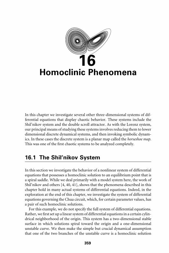
16Homoclinic Phenomena
In this chapter we investigate several other three-dimensional systems of dif-ferential equations that display chaotic behavior. These systems include theShil’nikov system and the double scroll attractor. As with the Lorenz system,our principal means of studying these systems involves reducing them to lowerdimensional discrete dynamical systems, and then invoking symbolic dynam-ics. In these cases the discrete system is a planar map called the horseshoe map.This was one of the first chaotic systems to be analyzed completely.
16.1 The Shil’nikov System
In this section we investigate the behavior of a nonlinear system of differentialequations that possesses a homoclinic solution to an equilibrium point that isa spiral saddle. While we deal primarily with a model system here, the work ofShil’nikov and others [4, 40, 41], shows that the phenomena described in thischapter hold in many actual systems of differential equations. Indeed, in theexploration at the end of this chapter, we investigate the system of differentialequations governing the Chua circuit, which, for certain parameter values, hasa pair of such homoclinic solutions.
For this example, we do not specify the full system of differential equations.Rather, we first set up a linear system of differential equations in a certain cylin-drical neighborhood of the origin. This system has a two-dimensional stablesurface in which solutions spiral toward the origin and a one-dimensionalunstable curve. We then make the simple but crucial dynamical assumptionthat one of the two branches of the unstable curve is a homoclinic solution
359

360 Chapter 16 Homoclinic Phenomena
and thus eventually enters the stable surface. We do not write down a specificdifferential equation having this behavior. Although it is possible to do so,having the equations is not particularly useful for understanding the globaldynamics of the system. In fact, the phenomena we study here depend onlyon the qualitative properties of the linear system described previously a keyinequality involving the eigenvalues of this linear system, and the homoclinicassumption.
The first portion of the system is defined in the cylindrical region S of R3
given by x2 + y2 ≤ 1 and |z | ≤ 1. In this region consider the linear system
X ′ =⎛⎝−1 1 0
−1 −1 00 0 2
⎞⎠X .
The associated eigenvalues are −1 ± i and 2. Using the results of Chapter 6,the flow φt of this system is easily derived:
x(t ) = x0e−t cos t + y0e−t sin t
y(t ) = −x0e−t sin t + y0e−t cos t
z(t ) = z0e2t .
Using polar coordinates in the xy–plane, solutions in S are given moresuccinctly by
r(t ) = r0e−t
θ(t ) = θ0 − t
z(t ) = z0e2t .
This system has a two-dimensional stable plane (the xy–plane) and a pair ofunstable curves ζ± lying on the positive and negative z-axis, respectively.
We remark that there is nothing special about our choice of eigenvalues forthis system. Everything below works fine for eigenvalues α ± iβ and λ whereα < 0, β �= 0, and λ > 0 subject only to the important condition that λ > −α.
The boundary of S consists of three pieces: the upper and lower disksD± given by z = ±1, r ≤ 1, and the cylindrical boundary C given byr = 1, |z | ≤ 1. The stable plane meets C along the circle z = 0 and dividesC into two pieces, the upper and lower halves given by C+ and C−, on whichz > 0 and z < 0, respectively. We may parametrize D± by r and θ and C by θ
and z . We will concentrate in this section on C+.Any solution of this system that starts in C+ must eventually exit from S
through D+. Hence we can define a map ψ1 : C+ → D+ given by followingsolution curves that start in C+ until they first meet D+. Given (θ0, z0) ∈ C+,

16.1 The Shil’nikov System 361
let τ = τ (θ0, z0) denote the time it takes for the solution through (θ0, z0) tomake the transit to D+. We compute immediately using z(t ) = z0e2t thatτ = − log(
√z0). Therefore
ψ1
⎛⎝ 1
θ0
z0
⎞⎠ =
⎛⎝r1
θ1
1
⎞⎠ =
⎛⎝
√z0
θ0 + log(√
z0)
1
⎞⎠ .
For simplicity, we will regard ψ1 as a map from the (θ0, z0) cylinder to the(r1, θ1) plane. Note that a vertical line given by θ0 = θ∗ in C+ is mapped byψ1 to the spiral
z0 → (√z0, θ∗ + log
(√z0))
,
which spirals down to the point r = 0 in D±, since log√
z0 → −∞ as z0 → 0.To define the second piece of the system, we assume that the branch ζ+
of the unstable curve leaving the origin through D+ is a homoclinic solution.That is, ζ+ eventually returns to the stable plane. See Figure 16.1. We assumethat ζ+ first meets the cylinder C at the point r = 1, θ = 0, z = 0. Moreprecisely, we assume that there is a time t1 such that φt1(0, θ , 1) = (1, 0, 0) inr , θ , z coordinates.
Therefore we may define a second map ψ2 by following solutions beginningnear r = 0 in D+ until they reach C . We will assume that ψ2 is, in fact,defined on all of D+. In Cartesian coordinates on D+, we assume that ψ2
takes (x , y) ∈ D+ to (θ1, z1) ∈ C via the rule
ψ2
(xy
)=
(θ1
z1
)=
(y/2x/2
).
f�
Figure 16.1 The homoclinic orbit ζ+.

362 Chapter 16 Homoclinic Phenomena
In polar coordinates, ψ2 is given by
θ1 = (r sin θ)/2
z1 = (r cos θ)/2.
Of course, this is a major assumption, since writing down such a map for aparticular nonlinear system would be virtually impossible.
Now the composition � = ψ2 ◦ ψ1 defines a Poincaré map on C+. Themap ψ1 is defined on C+ and takes values in D+, and then ψ2 takes values inC . We have � : C+ → C where
�
(θ0
z0
)=
(θ1
z1
)=
(12√
z0 sin(θ0 + log(
√z0)
)12√
z0 cos(θ0 + log(
√z0)
))
.
See Figure 16.2.As in the Lorenz system, we have now reduced the study of the flow of this
three-dimensional system to the study of a planar discrete dynamical system.As we shall see in the next section, this type of mapping has incredibly richdynamics that may be (partially) analyzed using symbolic dynamics. For a littletaste of what is to come, we content ourselves here with just finding the fixedpoints of �. To do this we need to solve
θ0 = 1
2
√z0 sin
(θ0 + log(
√z0)
)z0 = 1
2
√z0 cos
(θ0 + log(
√z0)
).
v2(D�)
f�
D�
C�
C�
Figure 16.2 The map ψ2 :D+ → C.

16.1 The Shil’nikov System 363
These equations look pretty formidable. However, if we square both equationsand add them, we find
θ20 + z2
0 = z0
4
so that
θ0 = ±1
2
√z0 − 4z2
0 ,
which is well defined provided that 0 ≤ z0 ≤ 1/4. Substituting this expressioninto the second equation above, we find that we need to solve
cos
(±1
2
√z0 − 4z2
0 + log(√
z0)) = 2
√z0.
Now the term√
z0 − 4z20 tends to zero as z0 → 0, but log(
√z0) → −∞.
Therefore the graph of the left-hand side of this equation oscillates infinitelymany times between ±1 as z0 → 0. Hence there must be infinitely manyplaces where this graph meets that of 2
√z0, and so there are infinitely many
solutions of this equation. This, in turn, yields infinitely many fixed points for�. Each of these fixed points then corresponds to a periodic solution of thesystem that starts in C+, winds a number of times around the z-axis near theorigin, and then travels around close to the homoclinic orbit until closing upwhen it returns to C+. See Figure 16.3.
f�c
Figure 16.3 A periodic solution γ
near the homoclinic solution ζ+.

364 Chapter 16 Homoclinic Phenomena
We now describe the geometry of this map; in the next section we use theseideas to investigate the dynamics of a simplified version of this map. First notethat the circles z0 = α in C+ are mapped by ψ1 to circles r = √
α centered atr = 0 in D+ since
ψ1
(θ0
α
)=
(r1
θ1
)=
( √α
θ0 + log(√
α)
).
Then ψ2 maps these circles to circles of radius√
α/2 centered at θ1 = z1 = 0in C . (To be precise, these are circles in the θz–plane; in the cylinder, thesecircles are “bent.”) In particular, we see that “one-half” of the domain C+ ismapped into the lower part of the cylinder C− and therefore no longer comesinto play.
Let H denote the half-disk �(C+) ∩ {z ≥ 0}. Half-disk H has center atθ1 = z1 = 0 and radius 1/2. The preimage of H in C+ consists of all points(θ0, z0) whose images satisfy z1 ≥ 0, so that we must have
z1 = 1
2
√z0 cos
(θ0 + log(
√z0)
) ≥ 0.
It follows that the preimage of H is given by
�−1(H ) = {(θ0, z0) | − π /2 ≤ θ0 + log(√
z0) ≤ π /2}where 0 < z0 ≤ 1. This is a region bounded by the two curves θ0 + log(
√z0) =
±π /2, each of which spirals downward in C+ toward the circle z = 0.See Figure 16.4. This follows since, as z0 → 0, we must have θ0 → ∞.More generally, consider the curves �α given by
θ0 + log(√
z0) = α
D�
C�
C�
H
Φ�1(H )
Figure 16.4 The half-disk H andits preimage in C+.

16.1 The Shil’nikov System 365
for −π /2 ≤ α ≤ π /2. These curves fill the preimage �−1(H ) and each spiralsaround C just as the boundary curves do. Now we have
�(�α) =√
z0
2
(sin α
cos α
),
so � maps each �α to a ray that emanates from θ = z = 0 in C+ and isparameterized by
√z0. In particular, � maps each of the boundary curves
�±π /2 to z = 0 in C .Since the curves �±π /2 spiral down toward the circle z = 0 in C , it follows
that �−1(H ) meets H in infinitely many strips, which are nearly horizontalclose to z = 0. See Figure 16.4. We denote these strips by Hk for k sufficientlylarge. More precisely, let Hk denote the component of �−1(H ) ∩ H for whichwe have
2kπ − 1
2≤ θ0 ≤ 2kπ + 1
2.
The top boundary of Hk is given by a portion of the spiral �π /2 and the bottomboundary by a piece of �−π /2. Using the fact that
−π
2≤ θ0 + log
(√z0) ≤ π
2,
we find that, if (θ0, z0) ∈ Hk , then
−(4k + 1)π − 1 ≤ −π − 2θ0 ≤ 2 log√
z0 ≤ π − 2θ0 ≤ −(4k − 1)π + 1
from which we conclude that
exp(−(4k + 1)π − 1) ≤ z0 ≤ exp(−(4k − 1)π + 1).
Now consider the image of Hk under �. The upper and lower boundariesof Hk are mapped to z = 0. The curves �α ∩ Hk are mapped to arcs in raysemanating from θ = z = 0. These rays are given as above by
√z0
2
(sin α
cos α
).
In particular, the curve �0 is mapped to the vertical line θ1 = 0, z1 = √z0/2.
Using the above estimate of the size of z0 in Hk , one checks easily that the imageof �0 lies completely above Hk when k ≥ 2. Therefore the image of �(Hk) is a“horseshoe-shaped” region that crosses Hk twice as shown in Figure 16.5. Inparticular, if k is large, the curves �α ∩ Hk meet the horsehoe �(Hk) in nearlyhorizontal subarcs.

366 Chapter 16 Homoclinic Phenomena
H Φ(Hk)
Hk
Figure 16.5 The image of Hk is ahorseshoe that crosses Hk twicein C +.
Such a map is called a horseshoe map; in the next section we discuss theprototype of such a function.
16.2 The Horseshoe Map
Symbolic dynamics, which played such a crucial role in our understanding ofthe one-dimensional logistic map, can also be used to study higher dimensionalphenomena. In this section, we describe an important example in R2, thehorseshoe map [43]. We shall see that this map has much in common with thePoincaré map described in the previous section.
To define the horseshoe map, we consider a region D consisting of threecomponents: a central square S with sides of length 1, together with twosemicircles D1 and D2 at the top and bottom. D is shaped like a “stadium.”
The horseshoe map F takes D inside itself according to the following pre-scription. First, F linearly contracts S in the horizontal direction by a factorδ < 1/2 and expands it in the vertical direction by a factor of 1/δ so that S islong and thin, and then F curls S back inside D in a horseshoe-shaped figureas displayed in Figure 16.6. We stipulate that F maps S linearly onto the twovertical “legs”of the horseshoe.
We assume that the semicircular regions D1 and D2 are mapped inside D1
as depicted. We also assume that there is a fixed point in D1 that attracts allother orbits in D1. Note that F(D) ⊂ D and that F is one-to-one. However,since F is not onto, the inverse of F is not globally defined. The remainder ofthis section is devoted to the study of the dynamics of F in D.
Note first that the preimage of S consists of two horizontal rectangles, H0
and H1, which are mapped linearly onto the two vertical components V0 andV1 of F(S) ∩ S. The width of V0 and V1 is therefore δ, as is the height of H0
and H1. See Figure 16.7. By linearity of F : H0 → V0 and F : H1 → V1, weknow that F takes horizontal and vertical lines in Hj to horizontal and verticallines in Vj for j = 1, 2. As a consequence, if both h and F(h) are horizontalline segments in S, then the length of F(h) is δ times the length of h. Similarly,

16.2 The Horseshoe Map 367
D1
D2
S F
F (D1) F (D2)
F(S)
Figure 16.6 The first iterate of the horseshoe map.
if v is a vertical line segment in S whose image also lies in S, then the length ofF(v) is 1/δ times the length of v .
We now describe the forward orbit of each point X ∈ D. Recall that theforward orbit of X is given by {Fn(X) | n ≥ 0}. By assumption, F has a uniquefixed point X0 in D1 and limn→∞Fn(X) = X0 for all X ∈ D1. Also, sinceF(D2) ⊂ D1, all forward orbits in D2 behave likewise. Similarly, if X ∈ S butFk(X) �∈ S for some k > 0, then we must have that Fk(X) ∈ D1 ∪ D2 so thatFn(X) → X0 as n → ∞ as well. Consequently, we understand the forwardorbits of any X ∈ D whose orbit enters D1, so it suffices to consider the set of
V0 V1
H1
H0
Figure 16.7 Therectangles H0 and H1 andtheir images V0 and V1 .

368 Chapter 16 Homoclinic Phenomena
points whose forward orbits never enter D1 and so lie completely in S. Let
�+ = {X ∈ S | Fn(X) ∈ S for n = 0, 1, 2, . . .}.
We claim that �+ has properties similar to the corresponding set for theone-dimensional logistic map described in Chapter 15.
If X ∈ �+, then F(X) ∈ S, so we must have that either X ∈ H0 or X ∈ H1,for all other points in S are mapped into D1 or D2. Since F2(X) ∈ S as well,we must also have F(X) ∈ H0 ∪H1, so that X ∈ F−1(H0 ∪H1). Here F−1(W )denotes the preimage of a set W lying in D. In general, since Fn(X) ∈ S, wehave X ∈ F−n(H0 ∪ H1). Thus we may write
�+ =∞⋂
n=0
F−n(H0 ∪ H1).
Now if H is any horizontal strip connecting the left and right boundaries ofS with height h, then F−1(H ) consists of a pair of narrower horizontal stripsof height δh, one in each of H0 and H1. The images under F of these narrowerstrips are given by H ∩ V0 and H ∩ V1. In particular, if H = Hi , F−1(Hi) is apair of horizontal strips, each of height δ2, with one in H0 and the other in H1.Similarly, F−1(F−1(Hi)) = F−2(Hi) consists of four horizontal strips, each ofheight δ3, and F−n(Hi) consists of 2n horizontal strips of width δn+1. Hencethe same procedure we used in Section 15.5 shows that �+ is a Cantor set ofline segments, each extending horizontally across S.
The main difference between the horseshoe and the logistic map is that, inthe horseshoe case, there is a single backward orbit rather than infinitely manysuch orbits. The backward orbit of X ∈ S is {F−n(X) | n = 1, 2, . . .}, providedF−n(X) is defined and in D. If F−n(X) is not defined, then the backwardorbit of X terminates. Let �− denote the set of points whose backward orbitis defined for all n and lies entirely in S. If X ∈ �−, then we have F−n(X) ∈ Sfor all n ≥ 1, which implies that X ∈ Fn(S) for all n ≥ 1. As above, this forcesX ∈ Fn(H0 ∪ H1) for all n ≥ 1. Therefore we may also write
�− =∞⋂
n=1
Fn(H0 ∪ H1).
On the other hand, if X ∈ S and F−1(X) ∈ S, then we must have X ∈F(S) ∩ S, so that X ∈ V0 or X ∈ V1. Similarly, if F−2(X) ∈ S as well, thenX ∈ F2(S) ∩ S, which consists of four narrower vertical strips, two in V0 andtwo in V1. In Figure 16.8 we show the image of D under F2. Arguing entirelyanalogously as above, it is easy to check that �− consists of a Cantor set ofvertical lines.

16.2 The Horseshoe Map 369
Figure 16.8 Thesecond iterate of thehorseshoe map.
Let
� = �+ ∩ �−
be the intersection of these two sets. Any point in � has its entire orbit (boththe backward and forward orbit) in S.
To introduce symbolic dynamics into this picture, we will assign a doublyinfinite sequence of 0’s and 1’s to each point in �. If X ∈ �, then, from theabove, we have
X ∈∞⋂
n=−∞Fn(H0 ∪ H1).
Thus we associate to X the itinerary
S(X) = (. . . s−2s−1 · s0s1s2 . . .)
where sj = 0 or 1 and sj = k if and only if Fj(X) ∈ Hk . This then provides uswith the symbolic dynamics on �. Let �2 denote the set of all doubly infinitesequences of 0’s and 1’s:
�2 = {(s) = (. . . s−2s−1 · s0s1s2 . . .) | sj = 0 or 1}.

370 Chapter 16 Homoclinic Phenomena
We impose a distance function on �2 by defining
d((s), (t)) =∞∑
i=−∞
|si − ti |2|i|
as in Section 15.5. Thus two sequences in �2 are “close” if they agree in all kspots where |k| ≤ n for some (large) n. Define the (two-sided) shift map σ by
σ (. . . s−2s−1 · s0s1s2 . . .) = (. . . s−2s−1s0 · s1s2 . . .).
That is, σ simply shifts each sequence in �2 one unit to the left (equivalently,σ shifts the decimal point one unit to the right). Unlike our previous (one-sided) shift map, this map has an inverse. Clearly, shifting one unit to the rightgives this inverse. It is easy to check that σ is a homeomorphism on �2 (seeExercise 2 at the end of this chapter).
The shift map is now the model for the restriction of F to �. Indeed, theitinerary map S gives a conjugacy between F on � and σ on �2. For if X ∈ �
and S(X) = (. . . s−2s−1 · s0s1s2 . . .), then we have X ∈ Hs0 , F(X) ∈ Hs1 ,F−1(X) ∈ Hs−1 , and so forth. But then we have F(X) ∈ Hs1 , F(F(X)) ∈ Hs2 ,X = F−1(F(X)) ∈ Hs0 , and so forth. This tells us that the itinerary of F(X) is(. . . s−1s0 · s1s2 . . .), so that
S(F(x)) = (. . . s−1s0 · s1s2 . . .) = σ (S(X)),
which is the conjugacy equation. We leave the proof of the fact that S is ahomeomorphism to the reader (see Exercise 3).
All of the properties that held for the old one-sided shift from the previouschapter hold for the two-sided shift σ as well. For example, there are precisely2n periodic points of period n forσ and there is a dense orbit forσ . Moreover, Fis chaotic on � (see Exercises 4 and 5). But new phenomena are present as well.We say that two points X1 and X2 are forward asymptotic if Fn(X1), Fn(X2) ∈ Dfor all n ≥ 0 and
limn→∞
∣∣Fn(X1) − Fn(X2)∣∣ = 0.
Points X1 and X2 are backward asymptotic if their backward orbits are definedfor all n and the above limit is zero as n → −∞. Intuitively, two points in Dare forward asymptotic if their orbits approach each other as n → ∞. Notethat any point that leaves S under forward iteration of F is forward asymptoticto the fixed point X0 ∈ D1. Also, if X1 and X2 lie on the same horizontal linein �+, then X1 and X2 are forward asymptotic. If X1 and X2 lie on the samevertical line in �−, then they are backward asymptotic.

16.2 The Horseshoe Map 371
We define the stable set of X to be
W s(X) = {Z ||Fn(Z ) − Fn(X)| → 0 as n → ∞}
.
The unstable set of X is given by
W u(X) = {Z ||F−n(X) − F−n(Z )| → 0 as n → ∞}
.
Equivalently, a point Z lies in W s(X) if X and Z are forward asymptotic.As above, any point in S whose orbit leaves S under forward iteration of thehorseshoe map lies in the stable set of the fixed point in D1.
The stable and unstable sets of points in � are more complicated. Forexample, consider the fixed point X∗, which lies in H0 and therefore has theitinerary (. . . 00 · 000 . . .). Any point that lies on the horizontal segment �s
through X∗ lies in W s(X∗). But there are many other points in this stable set.Suppose the point Y eventually maps into �s . Then there is an integer n suchthat |Fn(Y ) − X∗| < 1. Hence
|Fn+k(Y ) − X∗| < δk
and it follows that Y ∈ W s(X∗). Thus the union of horizontal intervals givenby F−k(�s) for k = 1, 2, 3, . . . all lie in W s(X∗). The reader may easily checkthat there are 2k such intervals.
Since F(D) ⊂ D, the unstable set of the fixed point X∗ assumes a somewhatdifferent form. The vertical line segment �u through X∗ in D clearly lies inW u(X∗). As above, all of the forward images of �u also lie in D. One mayeasily check that Fk(�u) is a “snake-like” curve in D that cuts vertically acrossS exactly 2k times. See Figure 16.9. The union of these forward images is thena very complicated curve that passes through S infinitely often. The closure ofthis curve in fact contains all points in � as well as all of their unstable curves(see Exercise 12).
The stable and unstable sets in � are easy to describe on the shift level. Let
s∗ = (. . . s∗−2s∗−1 · s∗0 s∗1 s∗2 . . .) ∈ �2.
Clearly, if t is a sequence whose entries agree with those of s∗ to the right ofsome entry, then t ∈ W s(s∗). The converse of this is also true, as is shown inExercise 6.
A natural question that arises is the relationship between the set � for theone-dimensional logistic map and the corresponding � for the horseshoe map.Intuitively, it may appear that the � for the horseshoe has many more points.However, both �’s are actually homeomorphic! This is best seen on the shiftlevel.

372 Chapter 16 Homoclinic Phenomena
X *
X0
Figure 16.9 The unstableset for X∗ in D.
Let �12 denote the set of one-sided sequences of 0’s and 1’s and �2 the set
of two-sided such sequences. Define a map
� : �12 → �2
by
�(s0s1s2 . . .) = (. . . s5s3s1 · s0s2s4 . . .).
It is easy to check that � is a homeomorphism between �12 and �2
(see Exercise 11).Finally, to return to the subject of Section 16.1, note that the return map
investigated in that section consists of infinitely many pieces that resemblethe horseshoe map of this section. Of course, the horseshoe map here waseffectively linear in the region where the map was chaotic, so the results inthis section do not go over immediately to prove that the return maps nearthe homoclinic orbit have similar properties. This can be done; however, thetechniques for doing so (involving a generalized notion of hyperbolicity) arebeyond the scope of this book. See [13] or [36] for details.
16.3 The Double Scroll Attractor
In this section we continue the study of behavior near homoclinic solutions ina three-dimensional system. We return to the system described in Section 16.1,

16.3 The Double Scroll Attractor 373
f�
f�
Figure 16.10 The homoclinic orbits ζ±.
only now we assume that the vector field is skew-symmetric about the origin. Inparticular, this means that both branches of the unstable curve at the orgin, ζ±,now yield homoclinic solutions as depicted in Figure 16.10. We assume thatζ+ meets the cylinder C given by r = 1, |z | ≤ 1 at the point θ = 0, z = 0,so that ζ− meets the cylinder at the diametrically opposite point, θ = π ,z = 0.
As in the Section 16.1, we have a Poincaré map � defined on the cylinder C .This time, however, we cannot disregard solutions that reach C in the regionz < 0; now these solutions follow the second homoclinic solution ζ− arounduntil they reintersect C . Thus � is defined on all of C − {z = 0}.
As before, the Poincaré map �+ defined in the top half of the cylinder, C+,is given by
�+(
θ0
z0
)=
(θ1
z1
)=
(12√
z0 sin(θ0 + log(
√z0)
)12√
z0 cos(θ0 + log(
√z0)
))
.
Invoking the symmetry, a computation shows that �− on C− is given by
�−(
θ0
z0
)=
(θ1
z1
)=
(π − 1
2
√−z0 sin(θ0 + log(
√−z0))
12
√−z0 cos(θ0 + log(
√−z0))
).
where z0 < 0 and θ0 is arbitrary. Hence �(C+) is the disk of radius 1/2 centeredat θ = 0, z = 0, while �(C−) is a similar disk centered at θ = π , z = 0.
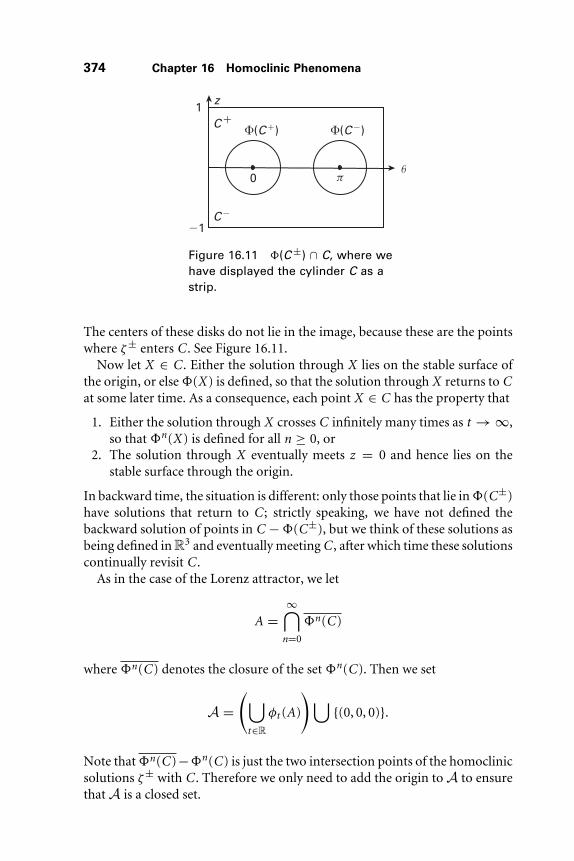
374 Chapter 16 Homoclinic Phenomena
C�
C�(C�)(C�)
0 oh
1
�1
z
Figure 16.11 �(C ±) ∩ C, where wehave displayed the cylinder C as astrip.
The centers of these disks do not lie in the image, because these are the pointswhere ζ± enters C . See Figure 16.11.
Now let X ∈ C . Either the solution through X lies on the stable surface ofthe origin, or else �(X) is defined, so that the solution through X returns to Cat some later time. As a consequence, each point X ∈ C has the property that
1. Either the solution through X crosses C infinitely many times as t → ∞,so that �n(X) is defined for all n ≥ 0, or
2. The solution through X eventually meets z = 0 and hence lies on thestable surface through the origin.
In backward time, the situation is different: only those points that lie in �(C±)have solutions that return to C ; strictly speaking, we have not defined thebackward solution of points in C − �(C±), but we think of these solutions asbeing defined in R3 and eventually meeting C , after which time these solutionscontinually revisit C .
As in the case of the Lorenz attractor, we let
A =∞⋂
n=0
�n(C)
where �n(C) denotes the closure of the set �n(C). Then we set
A =(⋃
t∈R
φt (A)
)⋃{(0, 0, 0)}.
Note that �n(C)−�n(C) is just the two intersection points of the homoclinicsolutions ζ± with C . Therefore we only need to add the origin to A to ensurethat A is a closed set.

16.4 Homoclinic Bifurcations 375
The proof of the following result is similar in spirit to the correspondingresult for the Lorenz attractor in Section 14.4.
Proposition. The set A has the following properties:
1. A is compact and invariant;2. There is an open set U containing A such that for each X ∈ U, φt (X) ∈ U
for all t ≥ 0 and ∩t≥0φt (U ) = A. �
Thus A has all of the properties of an attractor except the transitivity property.Nonetheless, A is traditionally called a double scroll attractor.
We cannot compute the divergence of the double scroll vector field as wedid in the Lorenz case for the simple reason that we have not written down theformula for this system. However, we do have an expression for the Poincarémap �. A straightforward computation shows that det D� = 1/8. That is,the Poincaré map � shrinks areas by a factor of 1/8 at each iteration. HenceA = ∩n≥0�n(C) has area 0 in C and we have:
Proposition. The volume of the double scroll attractor A is zero. �
16.4 Homoclinic Bifurcations
In higher dimensions, bifurcations associated with homoclinic orbits may leadto horribly (or wonderfully, depending on your point of view) complicatedbehavior. In this section we give a brief indication of some of the ramificationsof this type of bifurcation. We deal here with a specific perturbation of thedouble scroll vector field that breaks both of the homoclinic connections.
The full picture of this bifurcation involves understanding the “unfolding”of infinitely many horseshoe maps. By this we mean the following. Considera family of maps Fλ defined on a rectangle R with parameter λ ∈ [0, 1]. Theimage of Fλ(R) is a horseshoe as displayed in Figure 16.12. When λ = 0,Fλ(R) lies below R. As λ increases, Fλ(R) rises monotonically. When λ = 1,Fλ(R) crosses R twice and we assume that F1 is the horseshoe map describedin Section 16.2.
Clearly, F0 has no periodic points whatsoever in R, but by the time λ hasreached 1, infinitely many periodic points have been born, and other chaoticbehavior has appeared. The family Fλ has undergone infinitely many bifur-cations en route to the horseshoe map. How these bifurcations occur is thesubject of much contemporary research in mathematics.
The situation here is significantly more complex than the bifurcations thatoccur for the one-dimensional logistic family fλ(x) = λx(1− x) with 0 ≤ λ ≤4. The bifurcation structure of the logistic family has recently been completelydetermined; the planar case is far from being resolved.

376 Chapter 16 Homoclinic Phenomena
F0(R)
F1(R)
(a) (b)
b
aR
F0(b)
F1(b)F1(a)
F0(a)
Figure 16.12 The images Fλ(R) for (a) λ = 0 and(b) λ = 1.
We now introduce a parameter ε into the double scroll system. When ε = 0the system will be the double scroll system considered in the previous section.When ε �= 0 we change the system by simply translating ζ+ ∩ C (and thecorresponding transit map) in the z direction by ε. More precisely, we assumethat the system remains unchanged in the cylindrical region r ≤ 1, |z | ≤ 1,but we change the transit map defined on the upper disk D+ by adding (0, ε)to the image. That is, the new Poincaré map is given on C+ by
�+ε (θ , z) =
( 12
√z sin
(θ + log(
√z))
12
√z cos
(θ + log(
√z)) + ε
)
and �−ε is defined similarly using the skew-symmetry of the system. We further
assume that ε is chosen small enough (|ε| < 1/2) so that �±ε (C) ⊂ C .
When ε > 0, ζ+ intersects C in the upper cylindrical region C+ and then,after passing close to the origin, winds around itself before reintersecting Ca second time. When ε < 0, ζ+ now meets C in C− and then takes a verydifferent route back to C , this time winding around ζ−.
Recall that �+0 has infinitely many fixed points in C±. This changes
dramatically when ε �= 0.
Proposition. The maps �±ε each have only finitely many fixed points in C±
when ε �= 0.
Proof: To find fixed points of �+ε , we must solve
θ =√
z0
2sin
(θ + log(
√z))
z =√
z0
2cos
(θ + log(
√z)) + ε

16.4 Homoclinic Bifurcations 377
where ε > 0. As in Section 16.1, we must therefore have
z
4= θ2 + (z − ε)2
so that
θ = ±1
2
√z − 4(z − ε)2.
In particular, we must have
z − 4(z − ε)2 ≥ 0
or, equivalently,
4(z − ε)2
z≤ 1.
This inequality holds provided z lies in the interval Iε defined by
1
8+ ε − 1
8
√1 + 16ε ≤ z ≤ 1
8+ ε + 1
8
√1 + 16ε.
This puts a further restriction on ε for �+ε to have fixed points, namely,
ε > −1/16. Note that, when ε > −1/16, we have
1
8+ ε − 1
8
√1 + 16ε > 0
so that Iε has length√
1 + 16ε/4 and this interval lies to the right of 0.To determine the z-values of the fixed points, we must now solve
cos
(±1
2
√z − 4(z − ε)2 + log(
√z)
)= 2(z − ε)√
z
or
cos2(
±1
2
√z − 4(z − ε)2 + log(
√z)
)= 4(z − ε)2
z.
With a little calculus, one may check that the function
g (z) = 4(z − ε)2
z

378 Chapter 16 Homoclinic Phenomena
has a single minimum 0 at z = ε and two maxima equal to 1 at the endpointsof Iε . Meanwhile the graph of
h(z) = cos2(
±1
2
√z − 4(z − ε)2 + log(
√z)
)
oscillates between ±1 only finitely many times in Iε . Hence h(z) = g (z)at only finitely many z-values in Iε . These points are the fixed pointsfor �±
ε . �
Note that, as ε → 0, the interval Iε tends to [0, 1/4] and so the number ofoscillations of h in Iε increases without bound. Therefore we have
Corollary. Given N ∈ Z, there exists εN such that if 0 < ε < εN , then �+ε
has at least N fixed points in C+. �
When ε > 0, the unstable curve misses the stable surface in its first passthrough C . Indeed, ζ+ crosses C+ at θ = 0, z = ε. This does not mean thatthere are no homoclinic orbits when ε �= 0. In fact, we have the followingproposition:
Proposition. There are infinitely many values of ε for which ζ± arehomoclinic solutions that pass twice through C.
Proof: To show this, we need to find values of ε for which �+ε (0, ε) lies on
the stable surface of the origin. Thus we must solve
0 =√
ε
2cos
(0 − log(
√ε)) + ε
or
−2√
ε = cos(− log(
√ε))
.
But, as in Section 16.1, the graph of cos(− log√
ε) meets that of −2√
ε
infinitely often. This completes the proof. �
For each of the ε-values for which ζ± is a homoclinic solution, we again haveinfinitely many fixed points (for �±
ε ◦ �±ε ) as well as a very different structure
for the attractor. Clearly, a lot is happening as ε changes. We invite the readerwho has lasted this long with this book to go and figure out everything that ishappening here. Good luck! And have fun!

16.5 Exploration: The Chua Circuit 379
16.5 Exploration: The Chua Circuit
In this exploration, we investigate a nonlinear three-dimensional system ofdifferential equations related to an electrical circuit known as Chua’s circuit.These were the first examples of circuit equations to exhibit chaotic behavior.Indeed, for certain values of the parameters these equations exhibit behaviorsimilar to the double scroll attractor in Section 16.3. The original Chua circuitequations possess a piecewise linear nonlinearity. Here we investigate a varia-tion of these equations in which the nonlinearity is given by a cubic function.For more details on the Chua circuit, refer to [11] and [25].
The nonlinear Chua circuit system is given by
x ′ = a(y − φ(x))
y ′ = x − y + z
z ′ = −bz
where a and b are parameters and the function φ is given by
φ(x) = 1
16x3 − 1
6x .
Actually, the coefficients of this polynomial are usually regarded as parameters,but we will fix them for the sake of definiteness in this exploration. Whena = 10. 91865 . . . and b = 14, this system appears to have a pair of symmetrichomoclinic orbits as illustrated in Figure 16.13. The goal of this exploration
x
y
z
Figure 16.13 A pair of homoclinicorbits in the nonlinear Chua systemat parameter values a =10.91865. . . and b = 14.

380 Chapter 16 Homoclinic Phenomena
is to investigate how this system evolves as the parameter a changes. As aconsequence, we will also fix the parameter b at 14 and then let a vary. Wecaution the explorer that proving any of the chaotic or bifurcation behaviorobserved below is nearly impossible; virtually anything that you can do in thisregard would qualify as an interesting research result.
1. As always, begin by finding the equilibrium points.2. Determine the types of these equilibria, perhaps by using a computer
algebra system.3. This system possesses a symmetry; describe this symmetry and tell what
it implies for solutions.4. Let a vary from 6 to 14. Describe any bifurcations you observe as a varies.
Be sure to choose pairs of symmetrically located initial conditions in thisand other experiments in order to see the full effect of the bifurcations.Pay particular attention to solutions that begin near the origin.
5. Are there values of a for which there appears to be an attractor for thissystem? What appears to be happening in this case? Can you construct amodel?
6. Describe the bifurcation that occurs near the following a-values:
(a) a = 6. 58
(b) a = 7. 3
(c) a = 8. 78
(d) a = 10. 77
E X E R C I S E S
1. Prove that
d[(s), (t)] =∞∑
i=−∞
|si − ti |2|i|
is a distance function on �2, where �2 is the set of doubly infinitesequences of 0’s and 1’s as described in Section 16.2.
2. Prove that the shift σ is a homeomorphism of �2.3. Prove that S : � → �2 gives a conjugacy between σ and F .4. Construct a dense orbit for σ .5. Prove that periodic points are dense for σ .6. Let s∗ ∈ �2. Prove that W s(s∗) consists of precisely those sequences
whose entries agree with those of s∗ to the right of some entry of s∗.7. Let (0) = (. . . 00. 000 . . .) ∈ �2. A sequence s ∈ �2 is called homoclinic
to (0) if s ∈ W s(0) ∩ W u(0). Describe the entries of a sequence that is

Exercises 381
homoclinic to (0). Prove that sequences that are homoclinic to (0) aredense in �2.
8. Let (1) = (. . . 11. 111 . . .) ∈ �2. A sequence s is a heteroclinic sequence ifs ∈ W s(0)∩W u(1). Describe the entries of such a heteroclinic sequence.Prove that such sequences are dense in �2.
9. Generalize the definitions of homoclinic and heteroclinic points toarbitrary periodic points for σ and reprove Exercises 7 and 8 in thiscase.
10. Prove that the set of homoclinic points to a given periodic point iscountable.
11. Let �12 denote the set of one-sided sequences of 0’s and 1’s. Define
� : �12 → �2 by
�(s0s1s2 . . .) = (. . . s5s3s1 · s0s2s4 . . .).
Prove that � is a homeomorphism.12. Let X∗ denote the fixed point of F in H0 for the horseshoe map. Prove
that the closure of W u(X∗) contains all points in � as well as points ontheir unstable curves.
13. Let R : �2 → �2 be defined by
R(. . . s−2s−1. s0s1s2 . . .) = (. . . s2s1s0. s−1s−2 . . .).
Prove that R ◦ R = id and that σ ◦ R = R ◦ σ−1. Conclude thatσ = U ◦ R where U is a map that satisfies U ◦ U = id . Maps thatare their own inverses are called involutions. They represent very simpletypes of dynamical systems. Hence the shift may be decomposed into acomposition of two such maps.
14. Let s be a sequence that is fixed by R, where R is as defined in the previousexercise. Suppose that σ n(s) is also fixed by R. Prove that s is a periodicpoint of σ of period 2n.
15. Rework the previous exercise, assuming that σ n(s) is fixed by U , whereU is given as in Exercise 13. What is the period of s?
16. For the Lorenz system in Chapter 14, investigate numerically the bifur-cation that takes place for r between 13. 92 and 13. 96, with σ = 10 andb = 8/3.

This Page Intentionally Left Blank
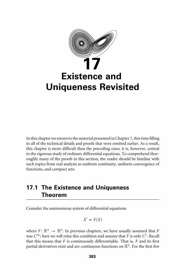
17Existence and
Uniqueness Revisited
In this chapter we return to the material presented in Chapter 7, this time fillingin all of the technical details and proofs that were omitted earlier. As a result,this chapter is more difficult than the preceding ones; it is, however, centralto the rigorous study of ordinary differential equations. To comprehend thor-oughly many of the proofs in this section, the reader should be familiar withsuch topics from real analysis as uniform continuity, uniform convergence offunctions, and compact sets.
17.1 The Existence and Uniqueness
Theorem
Consider the autonomous system of differential equations
X ′ = F(X)
where F : Rn → Rn . In previous chapters, we have usually assumed that Fwas C∞; here we will relax this condition and assume that F is only C1. Recallthat this means that F is continuously differentiable. That is, F and its firstpartial derivatives exist and are continuous functions on Rn . For the first few
383

384 Chapter 17 Existence and Uniqueness Revisited
sections of this chapter, we will deal only with autonomous equations; laterwe will assume that F depends on t as well as X .
As we know, a solution of this system is a differentiable function X : J → Rn
defined on some interval J ⊂ R such that for all t ∈ J
X ′(t ) = F(X(t )).
Geometrically, X(t ) is a curve in Rn whose tangent vector X ′(t ) equalsF(X(t )); as in previous chapters, we think of this vector as being based atX(t ), so that the map F : Rn → Rn defines a vector field on Rn . An initialcondition or initial value for a solution X : J → Rn is a specification of theform X(t0) = X0 where t0 ∈ J and X0 ∈ Rn . For simplicity, we usually taket0 = 0.
A nonlinear differential equation may have several solutions that satisfya given initial condition. For example, consider the first-order nonlineardifferential equation
x ′ = 3x2/3.
In Chapter 7 we saw that the identically zero function u0: R → R given byu0(t ) ≡ 0 is a solution satisfying the initial condition u(0) = 0. But u1(t ) = t 3
is also a solution satisfying this initial condition, and, in addition, for any τ > 0,the function given by
uτ (t ) ={
0 if t ≤ τ
(t − τ )3 if t > τ
is also a solution satisfying the initial condition uτ (0) = 0.Besides uniqueness, there is also the question of existence of solutions. When
we dealt with linear systems, we were able to compute solutions explicitly. Fornonlinear systems, this is often not possible, as we have seen. Moreover, certaininitial conditions may not give rise to any solutions. For example, as we sawin Chapter 7, the differential equation
x ′ ={
1 if x < 0−1 if x ≥ 0
has no solution that satisfies x(0) = 0.Thus it is clear that, to ensure existence and uniqueness of solutions, extra
conditions must be imposed on the function F . The assumption that F iscontinuously differentiable turns out to be sufficient, as we shall see. In thefirst example above, F is not differentiable at the problematic point x = 0,while in the second example, F is not continuous at x = 0.

17.2 Proof of Existence and Uniqueness 385
The following is the fundamental local theorem of ordinary differentialequations.
The Existence and Uniqueness Theorem. Consider the initial valueproblem
X ′ = F(X), X(0) = X0
where X0 ∈ Rn. Suppose that F : Rn → Rn is C1. Then there exists a uniquesolution of this initial value problem. More precisely, there exists a > 0 and aunique solution
X : (−a, a) → Rn
of this differential equation satisfying the initial condition
X(0) = X0. �
We will prove this theorem in the next section.
17.2 Proof of Existence and Uniqueness
We need to recall some multivariable calculus. Let F : Rn → Rn . Incoordinates (x1, . . . , xn) on Rn , we write
F(X) = (f1(x1, . . . , xn), . . . , fn(x1, . . . , xn)).
Let DFX be the derivative of F at the point X ∈ Rn . We may view this derivativein two slightly different ways. From one point of view, DFX is a linear mapdefined for each point X ∈ Rn ; this linear map assigns to each vector U ∈ Rn
the vector
DFX (U ) = limh→0
F(X + hU ) − F(X)
h,
where h ∈ R. Equivalently, from the matrix point of view, DFX is the n × nJacobian matrix
DFX =(
∂fi∂xj
)
where each derivative is evaluated at (x1, . . . , xn). Thus the derivative may beviewed as a function that associates different linear maps or matrices to eachpoint in Rn . That is, DF : Rn → L(Rn).

386 Chapter 17 Existence and Uniqueness Revisited
As earlier, the function F is said to be continuously differentiable, or C1, ifall of the partial derivatives of the fj exist and are continuous. We will assumefor the remainder of this chapter that F is C1. For each X ∈ Rn , we define thenorm |DFX | of the Jacobian matrix DFX by
|DFX | = sup|U |=1
|DFX (U )|
where U ∈ Rn . Note that |DFX | is not necessarily the magnitude of the largesteigenvalue of the Jacobian matrix at X .
Example. Suppose
DFX =(
2 00 1
).
Then, indeed, |DFX | = 2, and 2 is the largest eigenvalue of DFX . However, if
DFX =(
1 10 1
),
then
|DFX | = sup0≤θ≤2π
∣∣∣∣(
1 10 1
)(cos θ
sin θ
) ∣∣∣∣= sup
0≤θ≤2π
√(cos θ + sin θ)2 + sin2 θ
= sup0≤θ≤2π
√1 + 2 cos θ sin θ + sin2 θ
> 1
whereas 1 is the largest eigenvalue. �
We do, however, have
|DFX (V )| ≤ |DFX ||V |for any vector V ∈ Rn . Indeed, if we write V = (V /|V |) |V |, then we have
|DFX (V )| = ∣∣DFX(V /|V |)∣∣ |V | ≤ |DFX ||V |
since V /|V | has magnitude 1. Moreover, the fact that F : Rn → Rn is C1
implies that the function Rn → L(Rn), which sends X → DFX , is acontinuous function.

17.2 Proof of Existence and Uniqueness 387
Let O ⊂ Rn be an open set. A function F : O → Rn is said to be Lipschitzon O if there exists a constant K such that
|F(Y ) − F(X)| ≤ K |Y − X |for all X , Y ∈ O. We call K a Lipschitz constant for F . More generally, we saythat F is locally Lipschitz if each point in O has a neighborhood O′ in O suchthat the restriction F to O′ is Lipschitz. The Lipschitz constant of F |O′ mayvary with the neighborhoods O′.
Another important notion is that of compactness. We say that a set C ⊂ Rn
is compact if C is closed and bounded. An important fact is that, if f : C → R
is continuous and C is compact, then first of all f is bounded on C and,secondly, f actually attains its maximum on C. See Exercise 13 at the end of thischapter.
Lemma. Suppose that the function F : O → Rn is C1. Then F is locallyLipschitz.
Proof: Suppose that F : O → Rn is C1 and let X0 ∈ O. Let ε > 0 be so smallthat the closed ballOε of radius ε about X0 is contained inO. Let K be an upperbound for |DFX | on Oε ; this bound exists because DFX is continuous and Oε
is compact. The set Oε is convex ; that is, if Y , Z ∈ Oε , then the straight-linesegment connecting Y to Z is contained in Oε . This straight line is given byY + sU ∈ Oε , where U = Z − Y and 0 ≤ s ≤ 1. Let ψ(s) = F(Y + sU ).Using the chain rule we find
ψ ′(s) = DFY +sU (U ).
Therefore
F(Z ) − F(Y ) = ψ(1) − ψ(0)
=∫ 1
0ψ ′(s) ds
=∫ 1
0DFY +sU (U ) ds.
Thus we have
|F(Z ) − F(Y )| ≤∫ 1
0K |U | ds = K |Z − Y |. �
The following remark is implicit in the proof of the lemma: If O is convex,and if |DFX | ≤ K for all X ∈ O, then K is a Lipschitz constant for F |O.

388 Chapter 17 Existence and Uniqueness Revisited
Suppose that J is an open interval containing zero and X : J → O satisfies
X ′(t ) = F(X(t ))
with X(0) = X0. Integrating, we have
X(t ) = X0 +∫ t
0F(X(s)) ds.
This is the integral form of the differential equation X ′ = F(X). Conversely,if X : J → O satisfies this integral equation, then X(0) = X0 and X satisfiesX ′ = F(X), as is seen by differentiation. Thus the integral and differentialforms of this equation are equivalent as equations for X : J → O. To provethe existence of solutions, we will use the integral form of the differentialequation.
We now proceed with the proof of existence. Here are our assumptions:
1. Oρ is the closed ball of radius ρ > 0 centered at X0.2. There is a Lipschitz constant K for F on Oρ .3. |F(X)| ≤ M on Oρ .4. Choose a < min{ρ/M , 1/K } and let J = [−a, a].
We will first define a sequence of functions U0, U1, . . . from J to Oρ . Then wewill prove that these functions converge uniformly to a function satisfying thedifferential equation. Later we will show that there are no other such solutions.The lemma that is used to obtain the convergence of the Uk is the following:
Lemma from Analysis. Suppose Uk : J → Rn , k = 0, 1, 2, . . . is a sequenceof continuous functions defined on a closed interval J that satisfy: Given ε > 0,there is some N > 0 such that for every p, q > N
maxt∈J
|Up(t ) − Uq(t )| < ε.
Then there is a continuous function U : J → Rn such that
maxt∈J
|Uk(t ) − U (t )| → 0 as k → ∞.
Moreover, for any t with |t | ≤ a,
limk→∞
∫ t
0Uk(s) ds =
∫ t
0U (s) ds. �

17.2 Proof of Existence and Uniqueness 389
This type of convergence is called uniform convergence of the functions Uk .This lemma is proved in elementary analysis books and will not be provedhere. See [38].
The sequence of functions Uk is defined recursively using an iterationscheme known as Picard iteration. We gave several illustrative examples ofthis iterative scheme back in Chapter 7. Let
U0(t ) ≡ X0.
For t ∈ J define
U1(t ) = X0 +∫ t
0F(U0(s)) ds = X0 + tF(X0).
Since |t | ≤ a and |F(X0)| ≤ M , it follows that
|U1(t ) − X0| = |t ||F(X0)| ≤ aM ≤ ρ
so that U1(t ) ∈ Oρ for all t ∈ J . By induction, assume that Uk(t ) has beendefined and that |Uk(t ) − X0| ≤ ρ for all t ∈ J . Then let
Uk+1(t ) = X0 +∫ t
0F(Uk(s)) ds.
This makes sense since Uk(s) ∈ Oρ so the integrand is defined. We show that|Uk+1(t ) − X0| ≤ ρ so that Uk+1(t ) ∈ Oρ for t ∈ J ; this will imply that thesequence can be continued to Uk+2, Uk+3, and so on. This is shown as follows:
|Uk+1(t ) − X0| ≤∫ t
0|F(Uk(s))| ds
≤∫ t
0M ds
≤ Ma < ρ.
Next, we prove that there is a constant L ≥ 0 such that, for all k ≥ 0,∣∣Uk+1(t ) − Uk(t )∣∣ ≤ (aK )kL.
Let L be the maximum of |U1(t ) − U0(t )| over −a ≤ t ≤ a. By the above,L ≤ aM . We have
|U2(t ) − U1(t )| =∣∣∣∣∫ t
0F(U1(s)) − F(U0(s)) ds
∣∣∣∣

390 Chapter 17 Existence and Uniqueness Revisited
≤∫ t
0K |U1(s) − U0(s)| ds
≤ aKL.
Assuming by induction that, for some k ≥ 2, we have already proved
|Uk(t ) − Uk−1(t )| ≤ (aK )k−1L
for |t | ≤ a, we then have
|Uk+1(t ) − Uk(t )| ≤∫ t
0|F(Uk(s)) − F(Uk−1(s))| ds
≤ K
∫ t
0|Uk(s) − Uk−1(s)| ds
≤ (aK )(aK )k−1L
= (aK )kL.
Let α = aK , so that α < 1 by assumption. Given any ε > 0, we may choose Nlarge enough so that, for any r > s > N we have
|Ur (t ) − Us(t )| ≤∞∑
k=N
∣∣Uk+1(t ) − Uk(t )∣∣
≤∞∑
k=N
αkL
≤ ε
since the tail of the geometric series may be made as small as we please.By the lemma from analysis, this shows that the sequence of functions
U0, U1, . . . converges uniformly to a continuous function X : J → Rn . Fromthe identity
Uk+1(t ) = X0 +∫ t
0F(Uk(s)) ds,
we find by taking limits of both sides that
X(t ) = X0 + limk→∞
∫ t
0F(Uk(s)) ds

17.2 Proof of Existence and Uniqueness 391
= X0 +∫ t
0
(lim
k→∞F(Uk(s))
)ds
= X0 +∫ t
0F(X(s)) ds.
The second equality also follows from the Lemma from analysis. ThereforeX : J → Oρ satisfies the integral form of the differential equation and henceis a solution of the equation itself. In particular, it follows that X : J → Oρ
is C1.This takes care of the existence part of the theorem. Now we turn to the
uniqueness part.Suppose that X , Y : J → O are two solutions of the differential equation
satisfying X(0) = Y (0) = X0, where, as above, J is the closed interval [−a, a].We will show that X(t ) = Y (t ) for all t ∈ J . Let
Q = maxt∈J
|X(t ) − Y (t )|.
This maximum is attained at some point t1 ∈ J . Then
Q = |X(t1) − Y (t1)| =∣∣∣∣∫ t1
0(X ′(s) − Y ′(s)) ds
∣∣∣∣≤
∫ t1
0|F(X(s)) − F(Y (s))| ds
≤∫ t1
0K |X(s) − Y (s)| ds
≤ aKQ.
Since aK < 1, this is impossible unless Q = 0. Therefore
X(t ) ≡ Y (t ).
This completes the proof of the theorem. �
To summarize this result, we have shown: Given any ball Oρ ⊂ O of radiusρ about X0 on which
1. |F(X)| ≤ M ;2. F has Lipschitz constant K ; and3. 0 < a < min{ρ/M , 1/K };
there is a unique solution X : [−a, a] → O of the differential equation suchthat X(0) = X0. In particular, this result holds if F is C1 on O.

392 Chapter 17 Existence and Uniqueness Revisited
Some remarks are in order. First note that two solution curves of X ′ = F(X)cannot cross if F satisfies the hypotheses of the theorem. This is an imme-diate consequence of uniqueness but is worth emphasizing geometrically.Suppose X : J → O and Y : J1 → O are two solutions of X ′ = F(X) forwhich X(t1) = Y (t2). If t1 = t2 we are done immediately by the theorem.If t1 �= t2, then let Y1(t ) = Y (t2 − t1 + t ). Then Y1 is also a solution ofthe system. Since Y1(t1) = Y (t2) = X(t1), it follows that Y1 and X agreenear t1 by the uniqueness statement of the theorem, and hence so do X(t )and Y (t ).
We emphasize the point that if Y (t ) is a solution, then so too is Y1(t ) =Y (t + t1) for any constant t1. In particular, if a solution curve X : J → Oof X ′ = F(X) satisfies X(t1) = X(t1 + w) for some t1 and w > 0, then thatsolution curve must in fact be a periodic solution in the sense that X(t +w) =X(t ) for all t .
17.3 Continuous Dependence on Initial
Conditions
For the existence and uniqueness theorem to be at all interesting in any physicalor even mathematical sense, the result needs to be complemented by theproperty that the solution X(t ) depends continuously on the initial conditionX(0). The next theorem gives a precise statement of this property.
Theorem. Let O ⊂ Rn be open and suppose F : O → Rn has Lipschitzconstant K . Let Y (t ) and Z (t ) be solutions of X ′ = F(X) which remain in Oand are defined on the interval [t0, t1]. Then, for all t ∈ [t0, t1], we have
|Y (t ) − Z (t )| ≤ |Y (t0) − Z (t0)| exp(K (t − t0)). �
Note that this result says that, if the solutions Y (t ) and Z (t ) start out closetogether, then they remain close together for t near t0. While these solutionsmay separate from each other, they do so no faster than exponentially. Inparticular, we have this corollary:
Corollary. (Continuous Dependence on Initial Conditions) Letφ(t , X) be the flow of the system X ′ = F(X) where F is C1. Then φ is acontinuous function of X. �
The proof depends on a famous inequality that we prove first.

17.3 Continuous Dependence on Initial Conditions 393
Gronwall’s Inequality. Let u : [0, α] → R be continuous and nonnegative.Suppose C ≥ 0 and K ≥ 0 are such that
u(t ) ≤ C +∫ t
0Ku(s) ds
for all t ∈ [0, α]. Then, for all t in this interval,
u(t ) ≤ CeKt .
Proof: Suppose first that C > 0. Let
U (t ) = C +∫ t
0Ku(s) ds > 0.
Then u(t ) ≤ U (t ). Differentiating U , we find
U ′(t ) = Ku(t ).
Therefore,
U ′(t )U (t )
= Ku(t )
U (t )≤ K .
Hence
d
dt(log U (t )) ≤ K
so that
log U (t ) ≤ log U (0) + Kt
by integration. Since U (0) = C , we have by exponentiation
U (t ) ≤ CeKt ,
and so
u(t ) ≤ CeKt .
If C = 0, we may apply the above argument to a sequence of positive ci thattends to 0 as i → ∞. This proves Gronwall’s inequality. �
394 Chapter 17 Existence and Uniqueness Revisited
Proof: We turn now to the proof of the theorem. Define
v(t ) = |Y (t ) − Z (t )|.Since
Y (t ) − Z (t ) = Y (t0) − Z (t0) +∫ t
t0
(F(Y (s)) − F(Z (s))
)ds,
we have
v(t ) ≤ v(t0) +∫ t
t0
Kv(s) ds.
Now apply Gronwall’s inequality to the function u(t ) = v(t + t0) to get
u(t ) = v(t + t0) ≤ v(t0) +∫ t+t0
t0
Kv(s) ds
= v(t0) +∫ t
0Ku(τ ) dτ
so v(t + t0) ≤ v(t0) exp(Kt ) or v(t ) ≤ v(t0) exp(K (t − t0)), which is just theconclusion of the theorem. �
As we have seen, differential equations that arise in applications oftendepend on parameters. For example, the harmonic oscillator equations dependon the parameters b (the damping constant) and k (the spring constant); cir-cuit equations depend on the resistance, capacitance, and inductance; and soforth. The natural question is how do solutions of these equations depend onthese parameters? As in the previous case, solutions depend continuously onthese parameters provided that the system depends on the parameters in acontinuously differentiable fashion. We can see this easily by using a speciallittle trick. Suppose the system
X ′ = Fa(X)
depends on the parameter a in a C1 fashion. Let’s consider an “artificially”augmented system of differential equations given by
x ′1 = f1(x1, . . . , xn , a)
...x ′
n = fn(x1, . . . , xn , a)
a′ = 0.

17.4 Extending Solutions 395
This is now an autonomous system of n + 1 differential equations. While thisexpansion of the system may seem trivial, we may now invoke the previousresult about continuous dependence of solutions on initial conditions to verifythat solutions of the original system depend continuously on a as well.
Theorem. (Continuous Dependence on Parameters) Let X ′ = Fa(X)be a system of differential equations for which Fa is continuously differentiablein both X and a. Then the flow of this system depends continuously on a aswell as X . �
17.4 Extending Solutions
Suppose we have two solutions Y (t ), Z (t ) of the differential equation X ′ =F(X) where F is C1. Suppose also that Y (t ) and Z (t ) satisfy Y (t0) = Z (t0) andthat both solutions are defined on an interval J about t0. Now the existenceand uniqueness theorem guarantees that Y (t ) = Z (t ) for all t in an intervalabout t0 which may a priori be smaller than J . However, this is not the case. Tosee this, suppose that J ∗ is the largest interval on which Y (t ) = Z (t ). If J ∗ �= J ,there is an endpoint t1 of J ∗ and t1 ∈ J . By continuity, we have Y (t1) = Z (t1).Now the uniqueness part of the theorem guarantees that, in fact, Y (t ) andZ (t ) agree on an interval containing t1. This contradicts the assertion that J ∗is the largest interval on which the two solutions agree.
Thus we can always assume that we have a unique solution defined on amaximal time domain. There is, however, no guarantee that a solution X(t )can be defined for all time. For example, the differential equation
x ′ = 1 + x2,
has as solutions the functions x(t ) = tan(t − c) for any constant c . Such afunction cannot be extended over an interval larger than
c − π
2< t < c + π
2
since x(t ) → ±∞ as t → c ± π /2.Next, we investigate what happens to a solution as the limits of its domain
are approached. We state the result only for the right-hand limit; the othercase is similar.
Theorem. Let O ⊂ Rn be open, and let F : O → Rn be C1. Let Y (t ) be asolution of X ′ = F(X) defined on a maximal open interval J = (α, β) ⊂ R withβ < ∞. Then, given any compact set C ⊂ O, there is some t0 ∈ (α, β) withY (t0) �∈ C.

396 Chapter 17 Existence and Uniqueness Revisited
This theorem says that if a solution Y (t ) cannot be extended to a larger timeinterval, then this solution leaves any compact set in O. This implies that, ast → β, either Y (t ) accumulates on the boundary of O or else a subsequence|Y (ti)| tends to ∞ (or both).
Proof: Suppose Y (t ) ⊂ C for all t ∈ (α, β). Since F is continuous and C iscompact, there exists M > 0 such that |F(X)| ≤ M for all X ∈ C.
Let γ ∈ (α, β). We claim that Y extends to a continuous functionY : [γ , β] → C. To see this, it suffices to prove that Y is uniformly continuouson J . For t0 < t1 ∈ J we have
|Y (t0) − Y (t1)| =∣∣∣∣∫ t1
t0
Y ′(s) ds
∣∣∣∣≤
∫ t1
t0
|F(Y (s))| ds
≤ (t1 − t0)M .
This proves uniform continuity on J . Hence we may define
Y (β) = limt→β
Y (t ).
We next claim that the extended curve Y : [γ , β] → Rn is differentiable atβ and is a solution of the differential equation. We have
Y (β) = Y (γ ) + limt→β
∫ t
γ
Y ′(s) ds
= Y (γ ) + limt→β
∫ t
γ
F(Y (s)) ds
= Y (γ ) +∫ β
γ
F(Y (s)) ds.
where we have used uniform continuity of F(Y (s)). Therefore
Y (t ) = Y (γ ) +∫ t
γ
F(Y (s)) ds
for all t between γ and β. Hence Y is differentiable at β, and, in fact, Y ′(β) =F(Y (β)). Therefore Y is a solution on [γ , β]. Since there must then be asolution on an interval [β, δ) for some δ > β, we can extend Y to the interval(α, δ). Hence (α, β) could not have been a maximal domain of a solution. Thiscompletes the proof of the theorem. �

17.4 Extending Solutions 397
The following important fact follows immediately from this theorem.
Corollary. Let C be a compact subset of the open set O ⊂ Rn and letF : O → Rn be C1. Let Y0 ∈ C and suppose that every solution curve of theform Y : [0, β] → O with Y (0) = Y0 lies entirely in C. Then there is a solutionY : [0, ∞) → O satisfying Y (0) = Y0, and Y (t ) ∈ C for all t ≥ 0, so thissolution is defined for all (forward) time. �
Given these results, we can now give a slightly stronger theorem on thecontinuity of solutions in terms of initial conditions than the result discussedin Section 17.3. In that section we assumed that both solutions were defined onthe same interval. In the next theorem we drop this requirement. The theoremshows that solutions starting at nearby points are defined on the same closedinterval and also remain close to each other on this interval.
Theorem. Let F : O → Rn be C1. Let Y (t ) be a solution of X ′ = F(X) that isdefined on the closed interval [t0, t1], with Y (t0) = Y0. There is a neighborhoodU ⊂ Rn of Y0 and a constant K such that, if Z0 ∈ U, then there is a uniquesolution Z (t ) also defined on [t0, t1] with Z (t0) = Z0. Moreover Z satisfies
|Y (t ) − Z (t )| ≤ K |Y0 − Z0| exp(K (t − t0))
for all t ∈ [t0, t1]. �
For the proof we will need the following lemma.
Lemma. If F : O → Rn is locally Lipschitz and C ⊂ O is a compact set, thenF |C is Lipschitz.
Proof: Suppose not. Then for every k > 0, no matter how large, we can findX and Y in C with
|F(X) − F(Y )| > k|X − Y |.
In particular, we can find Xn , Yn such that
|F(Xn) − F(Yn)| ≥ n|Xn − Yn| for n = 1, 2, . . . .
Since C is compact, we can choose convergent subsequences of the Xn andYn . Relabeling, we may assume Xn → X∗ and Yn → Y ∗ with X∗ and Y ∗ in C.Note that we must have X∗ = Y ∗, since, for all n,
|X∗ − Y ∗| = limn→∞ |Xn − Yn| ≤ n−1|F(Xn) − F(Yn)| ≤ n−12M ,

398 Chapter 17 Existence and Uniqueness Revisited
where M is the maximum value of |F(X)| on C. There is a neighborhood O0
of X∗ on which F |O0 has Lipschitz constant K . Also there is an n0 such thatXn ∈ O0 if n ≥ n0. Therefore, for n ≥ n0,
|F(Xn) − F(Yn)| ≤ K |Xn − Yn|,which contradicts the assertion above for n > n0. This proves thelemma. �
Proof: The proof of the theorem now goes as follows: By compactness of[t0, t1], there exists ε > 0 such that X ∈ O if |X − Y (t )| ≤ ε for somet ∈ [t0, t1]. The set of all such points is a compact subset C of O. The C1 mapF is locally Lipschitz, as we saw in Section 17.2. By the lemma, it follows thatF |C has a Lipschitz constant K .
Let δ > 0 be so small that δ ≤ ε and δ exp(K |t1 − t0|) ≤ ε. We claim thatif |Z0 − Y0| < δ, then there is a unique solution through Z0 defined on all of[t0, t1]. First of all, Z0 ∈ O since |Z0 − Y (t0)| < ε, so there is a solution Z (t )through Z0 on a maximal interval [t0, β). We claim that β > t1. For supposeβ ≤ t1. Then, by Gronwall’s inequality, for all t ∈ [t0, β), we have
|Z (t ) − Y (t )| ≤ |Z0 − Y0| exp(K |t − t0|)≤ δ exp(K |t − t0|)≤ ε.
Thus Z (t ) lies in the compact set C. By the results above, [t0, β) couldnot be a maximal solution domain. Therefore Z (t ) is defined on [t0, t1].The uniqueness of Z (t ) then follows immediately. This completes theproof. �
17.5 Nonautonomous Systems
We turn our attention briefly in this section to nonautonomous differ-ential equations. Even though our main emphasis in this book has beenon autonomous equations, the theory of nonautonomous (linear) equa-tions is needed as a technical device for establishing the differentiability ofautonomous flows.
Let O ⊂ R × Rn be an open set, and let F : O → Rn be a function thatis C1 in X but perhaps only continuous in t . Let (t0, X0) ∈ O. Consider thenonautonomous differential equation
X ′(t ) = F(t , X), X(t0) = X0.

17.5 Nonautonomous Systems 399
As usual, a solution of this system is a differentiable curve X(t ) in Rn definedfor t in some interval J having the following properties:
1. t0 ∈ J and X(t0) = X0,2. (t , X(t )) ∈ O and X ′(t ) = F(t , X(t )) for all t ∈ J .
The fundamental local theorem for nonautonomous equations is as follows:
Theorem. Let O ⊂ R × Rn be open and F : O → Rn a function thatis C1 in X and continuous in t . If (t0, X0) ∈ O, there is an open interval Jcontaining t and a unique solution of X ′ = F(t , X) defined on J and satisfyingX(t0) = X0. �
The proof is the same as that of the fundamental theorem for autonomousequations (Section 17.2), the extra variable t being inserted where appropriate.An important corollary of this result follows:
Corollary. Let A(t ) be a continuous family of n × n matrices. Let (t0, X0) ∈J × Rn. Then the initial value problem
X ′ = A(t )X , X(t0) = X0
has a unique solution on all of J . �
For the proof, see Exercise 14 at the end of the chapter.We call the function F(t , X) Lipschitz in X if there is a constant K ≥ 0 such
that
|F (t , X1) − F (t , X2) | ≤ K |X1 − X2|for all (t , X1) and (t , X2) in O. Locally Lipschitz in X is defined analogously.
As in the autonomous case, solutions of nonautonomous equations arecontinuous with respect to initial conditions if F(t , X) is locally Lipschitz inX . We leave the precise formulation and proof of this fact to the reader.
A different kind of continuity is continuity of solutions as functions of thedata F(t , X). That is, if F : O → Rn and G : O → Rn are both C1 in X ,and |F − G| is uniformly small, we expect solutions to X ′ = F(t , X) andY ′ = G(t , Y ), having the same initial values, to be close. This is true; in fact,we have the following more precise result:
Theorem. Let O ⊂ R × Rn be an open set containing (0, X0) and supposethat F , G : O → Rn are C1 in X and continuous in t . Suppose also that for all(t , X) ∈ O,
|F(t , X) − G(t , X)| < ε.
400 Chapter 17 Existence and Uniqueness Revisited
Let K be a Lipschitz constant in X for F(t , X). If X(t ) and Y (t ) are solutions ofthe equations X ′ = F(t , X) and Y ′ = G(t , Y ), respectively, on some interval J,and X(0) = X0 = Y (0), then
|X(t ) − Y (t )| ≤ ε
K
(exp(K |t |) − 1
)for all t ∈ J .
Proof: For t ∈ J we have
X(t ) − Y (t ) =∫ t
0(X ′(s) − Y ′(s)) ds
=∫ t
0(F(s, X(s)) − G(s, Y (s))) ds.
Hence
|X(t ) − Y (t )| ≤∫ t
0|F(s, X(s)) − F(s, Y (s))| ds
+∫ t
0|F(s, Y (s)) − G(s, Y (s))| ds
≤∫ t
0K |X(s) − Y (s)| ds +
∫ t
0ε ds.
Let u(t ) = |X(t ) − Y (t )|. Then
u(t ) ≤ K
∫ t
0
(u(s) + ε
K
)ds,
so that
u(t ) + ε
K≤ ε
K+ K
∫ t
0
(u(s) + ε
K
)ds.
It follows from Gronwall’s inequality that
u(t ) + ε
K≤ ε
Kexp (K |t |) ,
which yields the theorem. �
17.6 Differentiability of the Flow
Now we return to the case of an autonomous differential equation X ′ = F(X)where F is assumed to be C1. Our aim is to show that the flow φ(t , X) = φt (X)

17.6 Differentiability of the Flow 401
determined by this equation is a C1 function of the two variables, and toidentify ∂φ/∂X . We know, of course, that φ is continuously differentiable inthe variable t , so it suffices to prove differentiability in X .
Toward that end let X(t ) be a particular solution of the system defined fort in a closed interval J about 0. Suppose X(0) = X0. For each t ∈ J let
A(t ) = DFX(t ).
That is, A(t ) denotes the Jacobian matrix of F at the point X(t ). Since F is C1,A(t ) is continuous. We define the nonautonomous linear equation
U ′ = A(t )U .
This equation is known as the variational equation along the solution X(t ).From the previous section we know that the variational equation has a solutionon all of J for every initial condition U (0) = U0. Also, as in the autonomouscase, solutions of this system satisfy the linearity principle.
The significance of this equation is that, if U0 is small, then the function
t → X(t ) + U (t )
is a good approximation to the solution X(t ) of the original autonomousequation with initial value X(0) = X0 + U0.
To make this precise, suppose that U (t , ξ) is the solution of the variationalequation that satisfies U (0, ξ) = ξ where ξ ∈ Rn . If ξ and X0 + ξ belong toO, let Y (t , ξ) be the solution of the autonomous equation X ′ = F(X) thatsatisfies Y (0) = X0 + ξ .
Proposition. Let J be the closed interval containing 0 on which X(t ) isdefined. Then
limξ→0
|Y (t , ξ) − X(t ) − U (t , ξ)||ξ |
converges to 0 uniformly for t ∈ J . �
This means that for every ε > 0, there exists δ > 0 such that if |ξ | ≤ δ, then
|Y (t , ξ) − (X(t ) + U (t , ξ))| ≤ ε|ξ |
for all t ∈ J . Thus as ξ → 0, the curve t → X(t ) + U (t , ξ) is a better andbetter approximation to Y (t , ξ). In many applications X(t ) + U (t , ξ) is usedin place of Y (t , ξ); this is convenient because U (t , ξ) is linear in ξ .

402 Chapter 17 Existence and Uniqueness Revisited
We will prove the proposition momentarily, but first we use this result toprove the following theorem:
Theorem. (Smoothness of Flows) The flow φ(t , X) of the autonomoussystem X ′ = F(X) is a C1 function; that is, ∂φ/∂t and ∂φ/∂X exist and arecontinuous in t and X.
Proof: Of course, ∂φ(t , X)/∂t is just F(φt (X)), which is continuous. Tocompute ∂φ/∂X we have, for small ξ ,
φ(t , X0 + ξ) − φ(t , X0) = Y (t , ξ) − X(t ).
The proposition now implies that ∂φ(t , X0)/∂X is the linear map ξ → U (t , ξ).The continuity of ∂φ/∂X is then a consequence of the continuity in initialconditions and data of solutions for the variational equation. �
Denoting the flow again by φt (X), we note that for each t the derivativeDφt (X) of the map φt at X ∈ O is the same as ∂φ(t , X)/∂X . We call this thespace derivative of the flow, as opposed to the time derivative ∂φ(t , X)/∂t .
The proof of the preceding theorem actually shows that Dφt (X) is the solu-tion of an initial value problem in the space of linear maps on Rn : for eachX0 ∈ O the space derivative of the flow satisfies the differential equation
d
dt(Dφt (X0)) = DFφt (X0)Dφt (X0),
with the initial condition Dφ0(X0) = I . Here we may regard X0 as a parameter.An important special case is that of an equilibrium solution X so that
φt (X) ≡ X . Putting DFX = A, we get the differential equation
d
dt(Dφt (X)) = ADφt (X),
with Dφ0(X) = I . The solution of this equation is
Dφt (X) = exp tA.
This means that, in a neighborhood of an equilibrium point, the flow isapproximately linear.
We now prove the proposition. The integral equations satisfied by X(t ),Y (t , ξ), and U (t , ξ) are
X(t ) = X0 +∫ t
0F(X(s)) ds,

17.6 Differentiability of the Flow 403
Y (t , ξ) = X0 + ξ +∫ t
0F(Y (s, ξ)) ds,
U (t , ξ) = ξ +∫ t
0DFX(s)(U (s, ξ)) ds.
From these we get, for t ≥ 0,
|Y (t ,ξ)−X(t )−U (t ,ξ)|≤∫ t
0|F(Y (s,ξ))−F(X(s))−DFX(s)(U (s,ξ))|ds.
The Taylor approximation of F at a point Z says
F(Y )=F(Z )+DFZ (Y −Z )+R(Z ,Y −Z ),
where
limY →Z
R(Z ,Y −Z )
|Y −Z | =0
uniformly in Z for Z in a given compact set. We apply this to Y =Y (s,ξ), Z =X(s). From the linearity of DFX(s) we get
|Y (t ,ξ)−X(t )−U (t ,ξ)|≤∫ t
0|DFX(s)(Y (s,ξ)−X(s)−U (s,ξ))|ds
+∫ t
0|R(X(s),Y (s,ξ)−X(s))|ds.
Denote the left side of this expression by g (t ) and set
N =max{|DFX(s)|| s ∈ J }.Then we have
g (t )≤N
∫ t
0g (s)ds+
∫ t
0|R(X(s),Y (s,ξ)−X(s))|ds.
Fix ε >0 and pick δ0 >0 so small that
|R(X(s),Y (s,ξ)−X(s))|≤ε|Y (s,ξ)−X(s)|if |Y (s,ξ)−X(s)|≤δ0 and s ∈ J .
From Section 17.3 there are constants K ≥0 and δ1 >0 such that
|Y (s,ξ)−X(s)|≤ |ξ |eKs ≤δ0
if |ξ |≤δ1 and s ∈ J .

404 Chapter 17 Existence and Uniqueness Revisited
Assume now that |ξ |≤δ1. From the previous equation, we find, for t ∈ J ,
g (t )≤N
∫ t
0g (s)ds+
∫ t
0ε|ξ |eKs ds,
so that
g (t )≤N
∫ t
0g (s)ds+Cε|ξ |
for some constant C depending only on K and the length of J . ApplyingGronwall’s inequality we obtain
g (t )≤CεeNt |ξ |
if t ∈ J and |ξ |≤δ1. (Recall that δ1 depends on ε.) Since ε is any positivenumber, this shows that g (t )/|ξ |→0 uniformly in t ∈ J , which proves theproposition.
E X E R C I S E S
1. Write out the first few terms of the Picard iteration scheme for each ofthe following initial value problems. Where possible, use any method tofind explicit solutions. Discuss the domain of the solution.
(a) x ′ =x−2;x(0)=1
(b) x ′ =x4/3;x(0)=0
(c) x ′ =x4/3;x(0)=1
(d) x ′ =cosx ;x(0)=0
(e) x ′ =1/2x ;x(1)=1
2. Let A be an n×n matrix. Show that the Picard method for solving X ′ =AX ,X(0)=X0 gives the solution exp(tA)X0.
3. Derive the Taylor series for cos t by applying the Picard method tothe first-order system corresponding to the second-order initial valueproblem
x ′′ =−x ; x(0)=1, x ′(0)=0.
4. For each of the following functions, find a Lipschitz constant on theregion indicated, or prove there is none:
(a) f (x)=|x|,−∞<x<∞(b) f (x)=x1/3,−1≤x ≤1

Exercises 405
(c) f (x)=1/x ,1≤x ≤∞(d) f (x ,y)= (x+2y ,−y),(x ,y)∈R2
(e) f (x ,y)= xy
1+x2+y2,x2+y2 ≤4
5. Consider the differential equation
x ′ =x1/3.
How many different solutions satisfy x(0)=0?6. What can be said about solutions of the differential equation x ′ =x/t ?7. Define f : R→R by f (x)=1 if x ≤1; f (x)=2 if x>1. What can be said
about solutions of x ′ = f (x) satisfying x(0)=1, where the right-hand sideof the differential equation is discontinuous? What happens if you haveinstead f (x)=0 if x>1?
8. Let A(t ) be a continuous family of n×n matrices and let P(t ) be thematrix solution to the initial value problem P ′ =A(t )P ,P(0)=P0. Showthat
detP(t )= (detP0)exp
(∫ t
0TrA(s)ds
).
9. Suppose F is a gradient vector field. Show that |DFX | is the magnitude ofthe largest eigenvalue of DFX . (Hint : DFX is a symmetric matrix.)
10. Show that there is no solution to the second-order two-point boundaryvalue problem
x ′′ =−x , x(0)=0, x(π)=1.
11. What happens if you replace the differential equation in the previousexercise by x ′′ =−kx with k>0?
12. Prove the following general fact (see also Section 17.3): If C ≥0 andu,v : [0,β]→R are continuous and nonnegative, and
u(t )≤C +∫ t
0u(s)v(s)ds
for all t ∈[0,β], then u(t )≤CeV (t ), where
V (t )=∫ t
0v(s)ds.
13. Suppose C ⊂Rn is compact and f :C →R is continuous. Prove thatf is bounded on C and that f attains its maximum value at somepoint in C.

406 Chapter 17 Existence and Uniqueness Revisited
14. Let A(t ) be a continuous family of n×n matrices. Let (t0,X0)∈ J ×Rn .Then the initial value problem
X ′ =A(t )X , X(t0)=X0
has a unique solution on all of J .15. In a lengthy essay not to exceed 50 pages, describe the behavior of all
solutions of the system X ′ =0 where X ∈Rn . Ah, yes. Another free andfinal gift from the Math Department.

Bibliography
1. Abraham, R., and Marsden, J. Foundations of Mechanics. Reading, MA:Benjamin-Cummings, 1978.
2. Abraham, R., and Shaw, C. Dynamics: The Geometry of Behavior. RedwoodCity, CA: Addison-Wesley, 1992.
3. Alligood, K., Sauer, T., and Yorke, J. Chaos: An Introduction to DynamicalSystems. New York: Springer-Verlag, 1997.
4. Afraimovich, V. S., and Shil’nikov, L. P. Strange attractors and quasiattractors.In Nonlinear Dynamics and Turbulence. Boston: Pitman, (1983), 1.
5. Arnold, V. I. Ordinary Differential Equations. Cambridge: MIT Press, 1973.6. Arnold, V. I. Mathematical Methods of Classical Mechanics. New York:
Springer-Verlag, 1978.7. Arrowsmith, D., and Place, C. An Introduction to Dynamical Systems.
Cambridge: Cambridge University Press, 1990.8. Banks, J. et al. On Devaney’s definition of chaos. Amer. Math. Monthly. 99
(1992), 332.9. Birman, J. S., and Williams, R. F. Knotted periodic orbits in dynamical systems
I: Lorenz’s equations. Topology. 22 (1983), 47.10. Blanchard, P., Devaney, R. L., and Hall, G. R. Differential Equations. Pacific
Grove, CA: Brooks-Cole, 2002.11. Chua, L., Komuro, M., and Matsumoto, T. The double scroll family. IEEE
Trans. on Circuits and Systems. 33 (1986), 1073.12. Coddington, E., and Levinson, N. Theory of Ordinary Equations. New York:
McGraw-Hill, 1955.13. Devaney, R. L. Introduction to Chaotic Dynamical Systems. Boulder, CO:
Westview Press, 1989.14. Devaney, K�. Math texts and digestion. J. Obesity. 23 (2002), 1.8.15. Edelstein-Keshet, L. Mathematical Models in Biology. New York: McGraw-
Hill, 1987.
407

408 References
16. Ermentrout, G. B., and Kopell, N. Oscillator death in systems of coupledneural oscillators. SIAM J. Appl. Math. 50 (1990), 125.
17. Field, R., and Burger, M., eds. Oscillations and Traveling Waves in ChemicalSystems. New York: Wiley, 1985.
18. Fitzhugh, R. Impulses and physiological states in theoretical models of nervemembrane. Biophys. J. 1 (1961), 445.
19. Golubitsky, M., Josic, K., and Kaper, T. An unfolding theory approach tobursting in fast-slow systems. In Global Theory of Dynamical Systems. Bristol,UK: Institute of Physics, 2001, 277.
20. Guckenheimer, J., and Williams, R. F. Structural stability of Lorenz attractors.Publ. Math. IHES. 50 (1979), 59.
21. Guckenheimer, J., and Holmes, P. Nonlinear Oscillations, Dynamical Systems,and Bifurcations of Vector Fields. New York: Springer-Verlag, 1983.
22. Gutzwiller, M. The anisotropic Kepler problem in two dimensions. J. Math.Phys. 14 (1973), 139.
23. Hodgkin, A. L., and Huxley, A. F. A quantitative description of membranecurrent and its application to conduction and excitation in nerves. J. Physiol.117 (1952), 500.
24. Katok, A., and Hasselblatt, B. Introduction to the Modern Theory of DynamicalSystems. Cambridge, UK: Cambridge University Press, 1995.
25. Khibnik, A., Roose, D., and Chua, L. On periodic orbits and homoclinicbifurcations in Chua’s circuit with a smooth nonlinearity. Int. J. Bifurcationand Chaos. 3 (1993), 363.
26. Kraft, R. Chaos, Cantor sets, and hyperbolicity for the logistic maps. Amer.Math Monthly. 106 (1999), 400.
27. Lengyel, I., Rabai, G., and Epstein, I. Experimental and modeling study ofoscillations in the chlorine dioxide–iodine–malonic acid reaction. J. Amer.Chem. Soc. 112 (1990), 9104.
28. Liapunov, A. M. The General Problem of Stability of Motion. London: Taylor& Francis, 1992.
29. Lorenz, E. Deterministic nonperiodic flow. J. Atmos. Sci. 20 (1963), 130.30. Marsden, J. E., and McCracken, M. The Hopf Bifurcation and Its Applications.
New York: Springer-Verlag, 1976.31. May, R. M. Theoretical Ecology: Principles and Applications. Oxford: Blackwell,
1981.32. McGehee, R. Triple collision in the collinear three body problem. Inventiones
Math. 27 (1974), 191.33. Moeckel, R. Chaotic dynamics near triple collision. Arch. Rational Mech. Anal.
107 (1989), 37.34. Murray, J. D. Mathematical Biology. Berlin: Springer-Verlag, 1993.35. Nagumo, J. S., Arimoto, S., and Yoshizawa, S. An active pulse transmission
line stimulating nerve axon. Proc. IRE. 50 (1962), 2061.36. Robinson, C. Dynamical Systems: Stability, Symbolic Dynamics, and Chaos.
Boca Raton, FL: CRC Press, 1995.37. Rössler, O. E. An equation for continuous chaos. Phys. Lett. A 57 (1976), 397.

References 409
38. Rudin, W. Principles of Mathematical Analysis. New York: McGraw-Hill, 1976.39. Schneider, G., and Wayne, C. E. Kawahara dynamics in dispersive media.
Phys. D 152 (2001), 384.40. Shil’nikov, L. P. A case of the existence of a countable set of periodic motions.
Sov. Math. Dokl. 6 (1965), 163.41. Shil’nikov, L. P. Chua’s circuit: Rigorous results and future problems. Int. J.
Bifurcation and Chaos. 4 (1994), 489.42. Siegel, C., and Moser, J. Lectures on Celestial Mechanics. Berlin: Springer-
Verlag, 1971.43. Smale, S. Diffeomorphisms with many periodic points. In Differential and
Combinatorial Topology. Princeton, NJ: Princeton University Press, 1965, 63.44. Sparrow, C. The Lorenz Equations: Bifurcations, Chaos, and Strange Attractors.
New York: Springer-Verlag, 1982.45. Strogatz, S. Nonlinear Dynamics and Chaos. Reading, MA: Addison-Wesley,
1994.46. Tucker, W. The Lorenz attractor exists. C. R. Acad. Sci. Paris Sér. I Math. 328
(1999), 1197.47. Winfree, A. T. The prehistory of the Belousov-Zhabotinsky reaction. J. Chem.
Educ. 61 (1984), 661.

This Page Intentionally Left Blank

Index
Pagenumbers followedby “f ” denote figures.
A
algebraequations, 26–29linear. see linear algebra
angular momentumconservation of, 283–284definition of, 283
anisotropic Kepler problem, 298–299answers
to all exercises, 1000.8, viiareal velocity, 284asymptotic stability, 175asymptotically stable, 175attracting fixed point, 329attractor
chaotic, 319–324description of, 310–311double scroll, 372–375Lorenz. see Lorenz attractorRössler, 324–325
autonomous, 5, 22
B
backward asymptotic, 370backward orbit, 320–321, 368basic regions, 190basin of attraction, 194, 200basis, 90Belousov-Zhabotinsky reaction, 231bifurcation
criterion, 333
definition of, 4, 8–9discrete dynamical systems, 332–335exchange, 334heteroclinic, 192–194homoclinic, 375–378Hopf, 181–182, 270–271, 308nonlinear systems, 176–182period doubling, 334, 335fpitchfork, 178–179, 179fsaddle-node, 177–178, 179f–180f, 181, 332tangent, 332
bifurcation diagram, 8biological applications
competition and harvesting, 252–253competitive species, 246–252infectious diseases, 235–239predator/prey systems, 239–246
blowing up the singularity, 293–297Bob. See Moe
C
canonical form, 49, 67, 84, 98, 111, 115Cantor middle-thirds set, 349–352capacitance, 260carrying capacity, 335Cauchy-Riemann equations, 184center
definition of, 44–47spiral, 112f
center of mass, 293central force fields, 281–284changing coordinates, 49–57
411

412 Index
chaoscubic, 352description of, 337–342
chaotic, 323chaotic attractor, 319–324characteristic, 259characteristic equation, 84chemical reactions, 230–231Chua circuit, 359, 379–380circuit theory applications
description of, 257neurodynamics, 272–273RLC circuit, 23, 257–261
classical mechanics, 277closed orbit
concepts for, 220–221definition of, 215Poincaré map, 221
coefficient matrix, 29collision surface, 295collision-ejection orbits, 288collision-ejection solutions, 296–297compact, 387compact set, 228–229competitive species applications, 246–252complex eigenvalues, 44–47, 54–55,
86–89configuration space, 278conjugacy equation, 340, 370conjugate, 340conservation of angular momentum,
283–284conservation of energy, 281conservative systems, 280–281constant coefficient equation, 25constant harvesting, 7–8constant of the motion, 208continuity, 70continuous dependence
of solutions, 147–149on initial conditions, 147–149,
392–395on parameters, 149, 395
continuous dynamical system, 141contracting condition, 316coordinates, changing of, 49–57critical point, 205cross product, 279cubic chaos, 352curve
definition of, 25local unstable, 169zero velocity, 286, 287f
D
damping constant, 26dense set, 101dense subset, 101determinant, 27, 81diffeomorphism, 66difference equation, 336differentiability of the flow, 400–404dimension, 91direction field, 24, 191fdiscrete dynamical systems
bifurcations, 332–335Cantor middle-thirds set, 349–352chaos, 337–342description of, 141, 327discrete logistic model, 335–337introduction to, 327–332one-dimensional, 320, 329orbits on, 329planar, 362shift map, 347–349symbolic dynamics, 342–347
discrete logistic model, 335–337discrete logistic population model, 336distance function, 344–345distinct eigenvalues, 75, 107–113divergence of vector field, 309dot product, 279double scroll attractor, 372–375doubling map, 338–339dynamical systems
discrete. see discrete dynamical systemsnonlinear, 140–142planar, 63–71, 222–225
E
eccentricity, 292eigenvalues
complex, 44–47, 54–55, 86–89definition of, 30, 83distinct, 75, 107–113eigenvectors and, relationship between, 30–33real distinct, 39–44, 51–53repeated, 47–49, 56–57, 95–101, 119–122
eigenvectorsdefinition of, 30, 83eigenvalues and, relationship between, 30–33
elementary matrix, 79–80elementary row operations, 79energy, 280energy surface, 286

Index 413
equationsalgebra, 26–29Cauchy-Riemann, 184characteristic, 84conjugacy, 340, 370constant coefficient, 25difference, 336first-order. see first-order equationsharmonic oscillator, 25–26homogeneous, 25, 131Lienard, 261–262Newton’s, 23nonautonomous, 10, 149–150, 160, 398–400second-order, 23van der Pol, 261–270variational, 149–153, 172, 401
equilibrium pointdefinition of, 2, 22, 174–175isolated, 206stability of, 194
equilibrium solution, 2errata. See Ki��er Devaney, viiiEuler’s method, 154exchange bifurcation, 334existence and uniqueness theorem
description of, 142–147, 383–385proof of, 385–392
expanding direction, 316exponential growth model, 335exponential of a matrix, 123–130extending solutions, 395–398
F
facesauthors’, 64masks, 313
Faraday’s law, 259first integral, 208first-order equations
description of, 1example of, 1–4logistic population model, 4–7Poincaré map. see Poincaré map
fixed pointattracting, 329description of, 328repelling, 330source, 330z-values, 377
flowdefinition of, 12, 64–65differentiability of, 400–404
gradient, 204smoothness of, 149–150, 402
flow box, 218–220force field
central, 281–284definition of, 277
forced harmonic oscillator, 23, 131forcing term, 130forward asymptotic, 370forward orbit, 320, 367free gift, 155, 406function
distance, 344–345Hamiltonian, 281Liapunov, 195, 200, 307total energy, 197
G
general solution, 34generic property, 104genericity, 101–104gradient, 204gradient systems, 203–207graphical iteration, 329Gronwall’s inequality, 393–394, 398
H
Hamiltonian function, 281Hamiltonian systems, 207–210, 281harmonic oscillator
description of, 114–119equation for, 25–26forced, 23, 131two-dimensional, 278undamped, 55, 114, 208
harvestingconstant, 7–8periodic, 9–11
heteroclinic bifurcation, 192–194heteroclinic solutions, 193higher dimensional saddles, 173–174Hodgkin-Huxley system, 272homeomorphism, 65, 69, 345homoclinic bifurcations, 375–378homoclinic orbits, 209, 361homoclinic solutions, 209, 226, 363fhomogeneous equation, 25, 131Hopf bifurcation, 181–182, 270–271, 308horseshoe map, 359, 366–372hyperbolic, 66, 166hyperbolicity condition, 316

414 Index
I
ideal pendulum, 208–209improved Euler’s method, 154inductance, 260infectious diseases, 235–239initial conditions
continuous dependence on, 147–149,392–395
definition of, 142, 384sensitive dependence on, 305, 321
initial value, 142, 384initial value problem, 2, 142inner product, 279invariant, 181, 199inverse matrix, 50, 79inverse square law, 285invertibility criterion, 82–83invertible, 50, 79–80irrational rotation, 118itinerary, 343, 369
J
Jacobian matrix, 149–150, 166, 401
K
Kepler’s lawsfirst law, 289–292proving of, 284
kernel, 92, 96Ki��er Devaney, viii, 407kinetic energy, 280, 290Kirchhoff’s current law, 258, 260Kirchhoff’s voltage law, 259
L
Lasalle’s invariance principle,200–203
latus rectum, 292law of gravitation, 285, 292lemma, 126–127, 318, 388–392Liapunov exponents, 323Liapunov function, 195, 200, 307Liapunov stability, 194Lienard equation, 261–262limit cycle, 227–228limit sets, 215–218linear algebra
description of, 75higher dimensional, 75–105preliminaries from, 75–83
linear combination, 28linear map, 50, 88, 92–93, 107linear pendulum, 196linear systems
description of, 29–30higher dimensional, 107–138nonautonomous, 130–135solving of, 33–36three-parameter family of, 71
linear transformation, 92linearity principle, 36linearization theorem, 168linearized system near X0, 166linearly dependent, 27, 76linearly independent, 27, 76Lipschitz constant, 387, 398Lipschitz in X , 399local section, 218local unstable curve, 169locally Lipschitz, 387logistic map, 336logistic population model, 4–7, 335Lorenz attractor
definition of, 305, 305fmodel for, 314–319properties of, 310–313, 374
Lorenz modeldescription of, 304dynamics of, 323–324
Lorenz systembehavior of, 310history of, 303–304introduction to, 304–305linearization, 312properties of, 306–310
Lorenz vector field, 306
M
matrixarithmetic, 78elementary, 79–80exponential of, 123–130Jacobian, 149–150, 166, 401reduced row echelon form of, 79square, 95sums, 78symmetric, 207
matrix formcanonical, 49, 67, 84, 98, 111, 115description of, 27
mechanical system with n degrees of freedom,278

Index 415
mechanicsclassical, 277conservative systems, 280–281Newton’s second law, 277–280
method of undetermined coefficients, 130metric, 344minimal period n, 328Moe. See Stevemomentum vector, 281monotone sequences, 222–225
N
n-cycles, 328near-collision solutions, 297neat picture, 305neurodynamics, 272–273Newtonian central force system
description of, 285–289problems, 297–298singularity, 293
Newton’s equation, 23Newton’s law of gravitation, 196, 285, 292Newton’s second law, 277–280nonautonomous differential equations, 10,
149–150, 160, 398–400nonautonomous linear systems, 130–135nonlinear pendulum, 196–199nonlinear saddle, 168–174nonlinear sink, 165–168nonlinear source, 165–168nonlinear systems
bifurcations, 176–182continuous dependence of solutions,
147–149description of, 139–140dynamical, 140–142equilibria in, 159–187existence and uniqueness theorem,
142–147global techniques, 189–214numerical methods, 153–156saddle, 168–174stability, 174–176variational equation, 149–153
nullclines, 189–194
O
Ohm’s law, 259–260one-dimensional discrete dynamical system,
320orbit
backward, 320–321, 368
closed. see Closed orbitdefinition of, 118forward, 320, 367homoclinic, 209, 361seed of the, 328, 338f
orbit diagram, 353–354origin
definition of, 164linearization at, 312unstable curve at, 313f
P
parameterscontinuous dependence on,
149, 395variation of, 130–131, 134
pendulumconstant forcing, 210–211ideal, 208–209linear, 196nonlinear, 196–199
period doubling bifurcation,334, 335f
periodic harvesting, 9–11periodic points
definition of, 322of period n, 328
periodic solution, 215, 363fphase line, 3phase plane, 41phase portraits
center, 46fdefinition of, 40repeated eigenvalues, 50frepeated real eigenvalues, 121fsaddle, 39–42sink, 42–43source, 43–44spiral center, 112fspiral sink, 48f
phase space, 278physical state, 259Picard iteration, 144–145, 389pitchfork bifurcation, 178–179, 179fplanar systems
description of, 24–26dynamical, 63–71, 222–225linear, 29–30local section, 221phase portraits for, 39–60Poincaré-Bendixson theorem. see
Poincaré-Bendixson theorem

416 Index
Poincaré map �, 319, 323, 373closed orbit, 221computing of, 12–15description of, 11, 221, 319graph of, 14semi-, 265
Poincaré-Bendixson theoremapplications of, 227–230, 246description of, 225–227
polar coordinates, 164population
discrete logistic population model, 336logistic population model, 4–7, 335
positive Liapunov exponents, 323positively invariant, 200potential energy, 280Prandtl number, 304predator/prey systems, 239–246
Q
quantum mechanical systems, 298–299quasi-periodic motions, 119
R
range, 92, 94Rayleigh number, 304real distinct eigenvalues, 39–44, 51–53reduced row echelon form, 79regular point, 205repeated eigenvalues, 47–49, 56–57, 95–101,
119–122repelling fixed point, 330resistor
characteristic, 259passive, 262
return condition, 316RLC circuit, 23, 257–261Rössler attractor, 324–325Runge-Kuta method, 154–155
S
saddledefinition of, 39–42, 108higher dimensional, 173–174nonlinear, 168–174spiral, 113
saddle connections, 193saddle-node bifurcation, 177–178, 179f–180f,
181, 332scaled variables, 294
second-order equations, 23seed of the orbit, 38f, 328semiconjugacy, 341semi-Poincaré map, 265sensitive dependence on initial conditions,
305, 321sensitivity constant, 338separation of variables, 241set
compact, 228–229dense, 101limit, 215–218
set of physical states, 259shift map, 347–349, 370Shil’nikov system, 359–366singularity, 293–297sink
definition of, 42–44, 329higher-dimensional, 109nonlinear, 165–168spiral, 47, 48fthree-dimensional, 110f
slope, 117slope field, 6smooth dynamical system, 141smoothness of flows, 149–150, 402S-nullclines, 236solutions
collision-ejection, 296–297continuous dependence of, 147–149equilibrium, 2extending, 395–398general, 34heteroclinic, 193homoclinic, 209, 226, 363fnear-collision, 297periodic, 215, 363fstraight-line, 33, 52
sourcedefinition of, 43–44nonlinear, 165–168spiral, 47, 48f
source fixed point, 330space
configuration, 278phase, 278state, 259, 278tangent, 286three-parameter, 71–72
space derivative, 402spanned, 77, 89spiral center, 112fspiral saddle, 113, 113f

Index 417
spiral sink, 47, 48fspiral source, 47, 48fspring constant, 26, 394square matrix, 95stability
asymptotic, 175equilibrium point, 194Liapunov, 194–196nonlinear systems, 174–176
stable curve, 161stable curve theorem, 168–169stable equilibrium, 175stable line, 40stable subspace, 108, 109fstandard basis, 28, 76state space, 259, 278Steve. See Bobstraight-line solution, 33, 52subspace
definition of, 77, 89–90stable, 108, 109funstable, 108, 109f
symbolic dynamics, 342–347symmetric matrix, 207
T
tangent bifurcation, 332tangent space, 286Taylor expansion, 166tent map, 339–340tertiary expansion, 351three-parameter space, 71–72threshold level, 238time derivative, 402time t map, 64torus, 116–117total energy, 280total energy function, 197trace-determinant plane, 61–63, 64f
transitive, 323two parameters, 15–16two-body problem, 292–293
U
undamped harmonic oscillator, 55,114, 208
uniform convergence, 389unrestricted voltage state, 259unstable curve, 169unstable line, 40unstable subspace, 108, 109f
V
van der Pol equation, 261–270variation of parameters, 130–131,
134variational equation, 149–153, 172,
401vector
definition of, 83momentum, 281
vector fieldcomplex, 182–184definition of, 24divergence of, 309Lorenz, 306
vector notation, 21–22Volterra-Lotka system, 240
W
web diagram, 331
Z
zero velocity curve, 286, 287f