INTERNATIONAL JOURNAL OF OPTIMIZATION IN CIVIL ENGINEERING

Int. J. Optim. Civil Eng., 2018; 8(2):311-328

DIFFERENT NEURAL NETWORKS AND MODAL TREE

METHOD FOR PREDICTING ULTIMATE BEARING CAPACITY

OF PILES

H. Harandizadeh1*, †, M. M. Toufigh1 and V. Toufigh2 1Department of Civil Engineering, Shahid Bahonar University of Kerman, 22 Bahman Blvd.,

Kerman, P.O.BOX: 76169133, Iran 2Department of Civil Engineering, Graduate University of Advanced Technology, Kerman,

P.O.BOX: 76315117, Iran

ABSTRACT

The prediction of the ultimate bearing capacity of the pile under axial load is one of the

important issues for many researches in the field of geotechnical engineering. In recent

years, the use of computational intelligence techniques such as different methods of artificial

neural network has been developed in terms of physical and numerical modeling aspects. In

this study, a database of 100 prefabricated steel and concrete piles is available from existing

publications to solve issues related to pile’s bearing capacity analysis. Three different

artificial neural network algorithms were developed for comparing and verifying the

obtained results at analyzing the bearing capacity of pile in soils. During the modeling

process, the geometric properties of different piles, soil materials properties, friction angle

and flap numbers (hammer blows) were selected as input parameters to the selected network

and the output from the network was considered as the bearing capacity of the pile. Finally,

the performance of radial base function type neural networks was compared with model tree

method and predictive neural networks based on different learning algorithms such as

Levenberg-Marquardt and Bayesian Regulation Back Propagation Algorithms. It was

observed that the radial base neural network in some cases achieved better results from

accuracy based on common statistical parameters such as correlation coefficient, mean

absolute error percentage and root mean square error as compared to other stated methods

and it showed the acceptable performance in modeling and predicting the desired output

close to the target's results.

Keywords: Pile Bearing Capacity, Deep Foundation, RBF Type Neural Network, Model

Tree, Levenberg Marquardt Learning Algorithm, Bayesian Regulation Learning Algorithm,

Multilayer Perceptron Neural Network

*Corresponding author: Department of Civil Engineering, Shahid Bahonar University of Kerman, 22

Bahman Blvd., Kerman, P.O.BOX: 76169133, Iran †E-mail address: hoomanharandizadeh@eng.uk.ac.ir (H. Harandizadeh)

Dow

nloa

ded

from

ijoc

e.iu

st.a

c.ir

at 5

:46

IRD

T o

n T

uesd

ay J

uly

31st

201

8

H. Harandizadeh, M. M. Toufigh and V. Toufigh 312

Received: 23 June 2017; Accepted: 2 September 2017

1. INTRODUCTION

Various methods and efforts have been made to determine the amount of ultimate bearing

capacity of deep foundation. The result of these researches is the presentation of formulas,

solutions or diagrams based on empirical methods of using plastic theory or numerical

methods. The disadvantage of semi-experimental methods and the method of plastic theory

in estimating the bearing capacity of deep foundation is the use of simplifying assumptions

which in most cases leads to a conservative estimate of the bearing capacity. Most of these

methods are set for homogeneous soil conditions or maximum two layers, which is not

compatible with the actual conditions of deep foundation.

Calculating the bearing capacity of deep foundation which are in layered soils has a more

complicated process than homogeneous or double-layered substrates. One of the reasons for

such complexities is the difference in the behavior of these soils against loading due to the

increase in the number of effective parameters on the bearing capacity compared to

homogeneous soils. In this paper, estimating the bearing capacity of deep foundation using

numerical modeling and artificial neural network technique has been investigated. Many

recent studies have been limited to develop numerical models in explaining the behavior of

foundations on layered soil based on element method.

Many researchers have investigated about the bearing capacity of piles and have achieved

various methods and formulas. Most of the methods estimate the bearing capacity

approximately by the mechanical parameters of the soil and the geometric characteristics of

the pile. Goh has used the length and diameter of the pile, the average effective stress, the

non-drain shear strength as network inputs and frictional surface strength as network outputs

to predict the bearing capacity of the pile [1]. The obtained results of the network by Semple

method, Rigden method and α method were compared and it was determined that the neural

network offers better responses in comparison with test and older methods. Also, Goh [2]

predicted the bearing capacity of slamming pile through the neural network. The used data

were the results of actual loading experiments on steel and concrete piles that were screwed

into sandy soils. When the model was evaluated by the test setup, it was seen that the

network is well able to model the bearing capacity of the pile. By measuring the synaptic

weights (connecting weights), it was determined that the main input factors are the weight

and type of hammer [1,2]. Lee and Lee [3] for the first time have predicted the bearing

capacity of pile using artificial neural networks. In his research, he used neural network back

propagation errors to predict the bearing capacity of the piles and was consistent with the

results of other experiments. The results indicate that the maximum error did not exceed

25%. Teh et al. [4] provided a network for estimating the static capacity of the pile

calculated by dynamic stress wave data for square-shaped piles made of prefabricated

concrete. The neural network fully absorbed the training data set and was able to predict the

ultimate capacity of the pile with a square average error of less than 0.0003 {Formatting

Citation}. Abu Kiefa [5] presented three models of the neural network (GRNNM3,

GRNNM2, GRNNM1) to determine the capacity of slamming pile in non-adhesive soils.

The first model was used to estimate the total bearing capacity of the pile, the second model

Dow

nloa

ded

from

ijoc

e.iu

st.a

c.ir

at 5

:46

IRD

T o

n T

uesd

ay J

uly

31st

201

8

DIFFERENT NEURAL NETWORKS AND MODAL TREE METHOD FOR …

313

was used to estimate the capacity of the pile tip and the third model was used to estimate the

lateral capacity of the pile. The obtained results of this study were compared with four

methods of (Meyerhof), (Coyle and Castello), American Petroleum Institute (API) and

(Randolph). The predicted results provided 0.95 for the Coefficient of Correlation by neural

networks while this number for the four methods mentioned above was in the range of 0.52

and 0.63 [5]. Hanna et al. [6] used the neural network to determine the efficiency of the pile

group in non-cohesive soils. Several static indicators such as R, MAE, RMSE and average

percentage error were calculated to evaluate the accuracy of the developed model. The

mentioned values for R (0.85), MAE (0.157), RMSE (0.232) and average percent error

(13%) indicate that the used neural network model had a high accuracy. Shahin et al. [6]

briefly outlined the application of artificial neural network in geotechnical engineering as

well as the accuracy of the neural network and the power of some artificial neural networks

[7, 8, 9]. Kordjezi and Pooyanejad [10] have used a machine learning method called support

vector machine (SVM) to predict the ultimate bearing capacity of piles under the influence

of axial load. Maizir and Kassin [11] used the collected data from approximately 300

projects in Indonesia and Malaysia for training and testing of artificial neural networks to

predict the axial bearing capacity of the slamming piles for the various pile characteristics

and the results of the slamming pile data analysis (PDA). McVay et al. [12] searched on pile

/ shaft design using an artificial neural network by genetic algorithm method (Genetic

programming) using Florida data and information based on the bearing capacity of the piles

(the wall and tip resistance of the pile), the internal friction angle (ø) and the extraction SPT

number of boreholes. Also, a lot of researches has been done on the application of artificial

intelligence algorithms [13,14] in other civil engineering fields (structural and geotechnical

engineering) in order to predict the parameters and optimizing earth, marine and space

structures. Kaveh et al. examined the optimization of structures by neural networks based on

the descending gradient learning algorithm [15]. In this study, a neural computing strategy

was developed to combine neural network information processing capabilities and structural

numerical optimization. In this strategy, an improved anti-imitation neural network was

used. Two artificial neural networks, one for constraints and another for constraint gradients

were trained and structural optimization was performed using these networks [16,17]. Kaveh

and Servati [18] evaluated the application of various neural networks for analyzing and

designing spatial structures used in existing buildings. Kaveh and Iranmanesh [17]

performed a comprehensive review of propagation neural networks and counter propagation

neural networks in the analysis and optimization of structures. Kaveh and Servati [18] have

been successfully performed the design of two-layer networks in spatial structures due to the

complexity and timing of calculations in analyzing and designing these structures using

backpropagation neural networks. Kaveh et al. [19] used BP neural networks for prediction

of moment-rotation characteristic for semi-rigid connections.Kaveh and Raiessi Dehkordi

[20] investigated some researches using BF and RBF neural networks for the analysis and

design of structural domes.

2. METHODS AND ASSUMPTION

The research method consists of three parts. In the first part of this study, there are the soil

Dow

nloa

ded

from

ijoc

e.iu

st.a

c.ir

at 5

:46

IRD

T o

n T

uesd

ay J

uly

31st

201

8

H. Harandizadeh, M. M. Toufigh and V. Toufigh 314

characteristics and the geometric properties of the pile obtained from the results of loading

pile test that were collected from published articles in some regions of Iran and regions of

different parts of the world. In the second part, computational artificial intelligence

techniques in geotechnical engineering related to the estimation of ultimate bearing capacity

were developed using radial network of neural function type, multi-layer perceptron

propagation algorithm and model tree. MATLAB was used in modeling and performing

current algorithms. In the third part of this study, input data into the neural network was

presented and optimized. Neural network architecture was trained to achieve the desired

goal. Neural network performance compared with each other about common statistical

parameters and finally the efficiency and performance of different models of artificial neural

network and model tree in calculating the ultimate pile capacity analysis was evaluated. The

range, precision and uniformity of the input data are very significant in achieving the output

results desired from the ANN model which is close to the actual values of the target.

Generally, an artificial neural network is a model that uses empirical data to create a logical

relationship between inputs and output data. Due to some collection limitations in this field

and empirical experiments, the existing published articles were used as referral materials. In

this study, input data were selected as geometric characteristics of the pile and soil layers

resistance parameters. The output of the numerical modeling network was considered as the

bearing capacity of the pile. The structure of the neural network system as well as the type of

transfer functions and the number of neurons in each layer using test and error to create

linear or nonlinear logical relationship between the input parameters of the network

(effective input variable) and the output parameter (target candle bearing capacity) and The

efficiency and reliability of the network were evaluated based on the correlation coefficient

and the network error was measured between the target value and the network output.

3. SOIL AND PILE INFORMATION

A database of 100 prefabricated concrete and steel piles was collected from existing papers

and publications. Geometric characteristics of the pile, mechanical properties of the soil,

number of flaps (number of hammer blows) and hammer blow energy for each individual

pile and also static loading test results for each pile were collected. Soil drainage cohesion,

drained soil friction angle and effective soil specific weight are variables that describe the

soil conditions. The cross-section area of the pile and the embedded length of pile are the

variables that describe the geometric properties of the pile. In addition to the variables

mentioned, the Flap number was used to determine all the effective hidden parameters in

calculating the bearing capacity of the pile. Seven variables were considered to predict the

bearing capacity of the pile:

A = cross-sectional area of the pile (m2)

C’= drained soil cohesion (KN / m2)

Number of Flap = multiplication of the number of hammer blows (N) in the relative

energy of the hammer (Er) for penetration of the pile in last one meter

L = the length of the embedded pile in the soil ' = Effective and specific weight of soil (KN / m3)

= Angle of friction between soil and pile (°)

Dow

nloa

ded

from

ijoc

e.iu

st.a

c.ir

at 5

:46

IRD

T o

n T

uesd

ay J

uly

31st

201

8

DIFFERENT NEURAL NETWORKS AND MODAL TREE METHOD FOR …

315

= internal friction angle of drained soil (°)

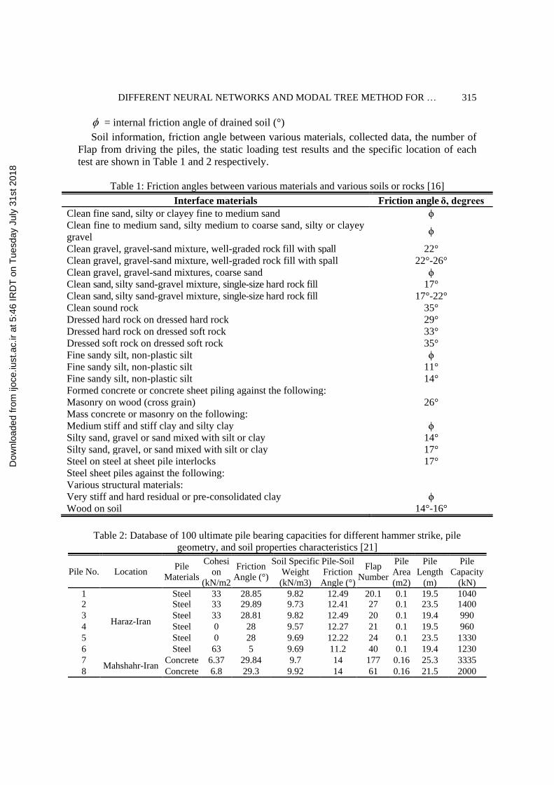
Soil information, friction angle between various materials, collected data, the number of

Flap from driving the piles, the static loading test results and the specific location of each

test are shown in Table 1 and 2 respectively.

Table 1: Friction angles between various materials and various soils or rocks [16]

Interface materials Friction angle δ, degrees

Clean fine sand, silty or clayey fine to medium sand ϕ

Clean fine to medium sand, silty medium to coarse sand, silty or clayey

gravel ϕ

Clean gravel, gravel-sand mixture, well-graded rock fill with spall 22°

Clean gravel, gravel-sand mixture, well-graded rock fill with spall 22°-26°

Clean gravel, gravel-sand mixtures, coarse sand ϕ

Clean sand, silty sand-gravel mixture, single-size hard rock fill 17°

Clean sand, silty sand-gravel mixture, single-size hard rock fill 17°-22°

Clean sound rock 35°

Dressed hard rock on dressed hard rock 29°

Dressed hard rock on dressed soft rock 33°

Dressed soft rock on dressed soft rock 35°

Fine sandy silt, non-plastic silt ϕ

Fine sandy silt, non-plastic silt 11°

Fine sandy silt, non-plastic silt 14°

Formed concrete or concrete sheet piling against the following:

Masonry on wood (cross grain) 26°

Mass concrete or masonry on the following:

Medium stiff and stiff clay and silty clay ϕ

Silty sand, gravel or sand mixed with silt or clay 14°

Silty sand, gravel, or sand mixed with silt or clay 17°

Steel on steel at sheet pile interlocks 17°

Steel sheet piles against the following:

Various structural materials:

Very stiff and hard residual or pre-consolidated clay ϕ

Wood on soil 14°-16°

Table 2: Database of 100 ultimate pile bearing capacities for different hammer strike, pile

geometry, and soil properties characteristics [21]

Pile No. Location Pile

Materials

Cohesi

on

(kN/m2

)

Friction

Angle (°)

Soil Specific

Weight

(kN/m3)

Pile-Soil

Friction

Angle (°)

Flap

Number

Pile

Area

(m2)

Pile

Length

(m)

Pile

Capacity

(kN)

1

Haraz-Iran

Steel 33 28.85 9.82 12.49 20.1 0.1 19.5 1040 2 Steel 33 29.89 9.73 12.41 27 0.1 23.5 1400

3 Steel 33 28.81 9.82 12.49 20 0.1 19.4 990

4 Steel 0 28 9.57 12.27 21 0.1 19.5 960

5 Steel 0 28 9.69 12.22 24 0.1 23.5 1330

6 Steel 63 5 9.69 11.2 40 0.1 19.4 1230

7 Mahshahr-Iran

Concrete 6.37 29.84 9.7 14 177 0.16 25.3 3335

8 Concrete 6.8 29.3 9.92 14 61 0.16 21.5 2000

Dow

nloa

ded

from

ijoc

e.iu

st.a

c.ir

at 5

:46

IRD

T o

n T

uesd

ay J

uly

31st

201

8

H. Harandizadeh, M. M. Toufigh and V. Toufigh 316

Pile No. Location Pile

Materials

Cohesi

on

(kN/m2

)

Friction

Angle (°)

Soil Specific

Weight

(kN/m3)

Pile-Soil

Friction

Angle (°)

Flap

Number

Pile

Area

(m2)

Pile

Length

(m)

Pile

Capacity

(kN)

9 Concrete 6.4 29.78 9.73 14 180 0.16 24.9 3142

10 Concrete 7 29 10.03 14 80 0.16 19.9 2520

11 Concrete 6.64 29.48 9.84 14 115 0.16 22.7 2840

12 Concrete 6.4 29.8 9.72 14 250 0.16 25 3867

13 Concrete 6.34 29.87 9.69 14 202 0.16 25.6 4012

14 Concrete 6.65 29.46 9.85 14 69 0.16 22.6 2278

15 Concrete 7 29 10.34 14 50 0.16 15.2 1900

16

Mahshahr-Iran

Concrete 138 4.23 7.52 14 246 0.16 22.9 2500

17 Concrete 142 4.14 7.55 14 210 0.16 23.4 2250

18 Concrete 148 4.03 7.58 14 306 0.16 24 2700

19 Gulf of Mexico

(Stockard,

1979)

Steel 8.7 24 8.55 11.75 790 0.89 61 19000

20 Steel 7.72 26.04 9.54 12.84 632 0.89 82 24900

21

India (Stockard,

1986)

Steel 1.4 29.39 9.1 13.75 1360 1.59 98 48470

22 Steel 1.58 27.67 8.66 12.68 1300 1.17 98 36250

23 Steel 4.87 26.77 8.81 12.1 2130 1.59 98 52100

24 Steel 2.76 28.39 8.93 13.12 1750 1.59 90 49350

25

Alton-Illinois

(Larry, 1988)

Steel 7.47 35.99 12.91 16.68 178 0.1 18 5900

26 Steel 6.59 35.64 12.92 16.13 178 0.1 20.4 6200

27 Steel 6.71 35.69 12.92 16.2 180 0.1 20 6120

28 Steel 7.78 36.62 13.19 17 86 0.1 16.1 4280

29 Steel 7.78 36.62 13.15 17 70 0.1 16.4 3130

30 Steel 7.83 36.56 13.49 17 29 0.07 14.2 1321

31 Steel 7.83 36.57 13.46 17 63 0.1 14.4 1300

32 Steel 7.79 36.6 13.27 17 49 0.13 15.6 1830

33 Illinois

(Fellenius,

1989)

Steel 14.6 32.22 9.89 13.75 16 0.16 15.2 1043

34 Steel 14.6 32.22 9.89 13.75 15 0.1 15.2 987

35

Bandar Imam-

Iran

Concrete 51.4 0 11.19 14 361 0.16 24.5 2030

36 Concrete 26 0 11.68 14 110 0.16 16 1145

37 Concrete 54.8 0 11.15 14 482 0.16 25.9 2250

38 Concrete 0.07 22.43 11.33 15.45 328 0.16 25.5 2600

39 Concrete 0.06 23.79 11.26 15.51 202 0.16 28.5 2200

40

Bandar Imam-

Iran

Concrete 51.8 11.81 7.3 14.88 234 0.16 26.5 2920

41 Concrete 51 12.24 7.36 15.02 263 0.16 27.2 2880

42 Concrete 58.6 11.43 8.34 14.59 112 0.16 14.5 680

43 Concrete 58.5 11.38 8.29 14.58 78 0.16 14.7 540

44

Shiraz-Iran

Concrete 136 27.82 8.94 14 167 0.16 18.2 2100

45 Concrete 137 27.1 8.84 14 94 0.16 19.5 1700

46 Concrete 138 29.3 9.21 14 98 0.16 15.9 2200

47 Ontario

(Fellenius and

Altaee, 2002)

Steel 18.2 20 5.45 13.75 78 0.09 60 2750

48 Steel 17.9 19.76 5.43 13.82 87 0.09 62 2870

49 Steel 17 18.93 − 5−.38 14.07 96 0.09 70 3050

50 Bandar Abbas-

Iran Steel 45.8 31.11 11.23 10.14 406 0.78 20.5 2670

51 Steel 49.8 31.01 11.2 12.47 670 1.16 22.5 3350

52 Steel 45.8 31.11 11.23 10.14 730 0.78 20.5 3750

53 Steel 45.8 31.11 11.23 10.14 1236 0.78 20.5 4100

54 Steel 45.8 31.11 11.23 10.14 710 0.78 20.5 3450

55 Steel 45.2 31.12 11.23 12.63 756 0.78 20.2 3570

Dow

nloa

ded

from

ijoc

e.iu

st.a

c.ir

at 5

:46

IRD

T o

n T

uesd

ay J

uly

31st

201

8

DIFFERENT NEURAL NETWORKS AND MODAL TREE METHOD FOR …

317

Pile No. Location Pile

Materials

Cohesi

on

(kN/m2

)

Friction

Angle (°)

Soil Specific

Weight

(kN/m3)

Pile-Soil

Friction

Angle (°)

Flap

Number

Pile

Area

(m2)

Pile

Length

(m)

Pile

Capacity

(kN)

56 Steel 48.8 31.03 11.21 12.5 1030 1.16 22 3570

57 Steel 44.7 31.14 11.24 12.65 1463 1.16 20 4936

58 Steel 51.5 30.97 11.2 12.4 1448 1.16 23.5 4900

59 Steel 49.8 31.01 11.2 12.47 1298 1.16 22.5 4650

60 Steel 41.1 31.23 11.25 12.78 1610 1.16 18.5 2150

61 Steel 42.4 31.2 11.24 12.74 1590 1.16 19 4150

62 Steel 45.8 31.11 11.23 10.14 701 0.89 20.5 3600

63 Steel 44.7 31.14 11.24 12.65 1112 0.89 20 4000

64 Steel 49.8 31.01 11.2 12.47 990 1.16 22.5 3870

65 Bandar Imam-

Iran Concrete 8.21 25.02 9.045 12.295 510 0.89 71.5 21965

66 Concrete 6.58 29.57 9.81 14 65 0.16 23.4 2682.5

67 Concrete 6.7 29.39 9.88 14 72 0.16 22.4 2846

68 Concrete 6.52 29.64 9.78 14 97 0.16 23.8 3368.5

69 Concrete 7.03 35.815 12.915 16.405 423 0.1 19.2 6065

70 Concrete 6.49 29.665 9.77 14 70 0.16 24.1 3160

71 Concrete 8.59 16.615 8.93 14 113 0.16 19 2215

72 Concrete 9.2 4.083 7.565 14 186 0.16 23.7 2490

73 Concrete 7.24 36.155 13.055 16.6 321 0.1 18.1 5215

74 Concrete 7.8 36.59 13.32 17 116 0.08 15.3 2240.5

75 Concrete 7.81 36.585 13.365 17 132 0.11 15 1580

76 Mahshahr-Iran Steel 24.6 32.22 9.89 13.75 56 0.13 15.2 1030

77 Steel 33.7 0 11.432 14 306 0.16 20.2 1602.5

78 Steel 27.4 11.215 11.24 14.725 505 0.16 25.7 2440

79 Steel 21.49 28.53 8.88 13.215 1106 1.38 32.2 4275

80 Steel 23.81 27.58 8.8715 12.61 1323 1.59 36.5 5740

81 Steel 25.9 17.8 9.28 15.195 196 0.16 27.5 2575

82 Steel 27.4 19.6 8.615 14.29 153 0.16 16.4 1335

83 Isfahan-Iran Concrete 38 28.2 9.025 14 196 0.16 23.7 1965

84 Concrete 28.1 19.88 5.44 13.785 70 0.09 27 2825

85 Concrete 31.4 25.02 8.305 12.105 725 0.44 25 2875

86 Concrete 45.8 31.11 11.23 10.14 2291 0.78 35.5 3790

87 Concrete 54.8 11.835 7.85 14.805 123 0.16 37.8 1795

88 Bandar Abbas-

Iran Steel 47.8 31.06 11.215 11.305 1631 0.97 21.5 3565

89 Steel 47 31.075 11.22 12.565 2078 0.97 21.1 3585

90 Steel 48.1 31.055 11.217 12.525 2147 1.16 21.7 3870

91 Steel 45.4 31.12 10.967 12.625 2243 1.16 20.5 3415

92 Steel 44.1 31.155 11.235 11.44 1009 1.02 19.7 5465

93 Steel 49.8 31.01 11.2 12.47 849 1.16 22.5 4275

94 Steel 31.1 34.42 11.54 15.375 131 0.1 15.7 2648.5

95 Steel 29.6 18.31 12.17 15.5 291 0.13 20.4 2595

96 Isfahan-Iran Concrete 33 29.37 9.775 12.45 14 0.1 21.5 1235

97 Concrete 28.5 28.405 9.695 12.38 14 0.1 19.4 1145

98 Concrete 31.5 16.5 − 9−.69 11.71 22 0.1 21.4 1295

99 Concrete 26.9 18.28 12.582 15.5 131 0.11 15.1 1248

100 Concrete 31.3 18.285 12.305 15.5 320 0.13 20.1 1790

Dow

nloa

ded

from

ijoc

e.iu

st.a

c.ir

at 5

:46

IRD

T o

n T

uesd

ay J

uly

31st

201

8

H. Harandizadeh, M. M. Toufigh and V. Toufigh 318

4. BASIC CONCEPTS

4.1 Framework of MLP and RBF neural networks

An artificial neural network is formed of input, hidden and output layers, hence it is known

as a three-layer network. The input layer contains independent variables that are attached to

the hidden layer for processing. The hidden layer contains activation functions and

calculates the weight of the variables in order to explore the predictive effects on the target

variables. In the output layer, the process of forecasting or classification ends and the results

are presented with the estimation of a small error. Generally, a back propagation algorithm

trains a predictive neural network. In the training sessions, the back propagation algorithm

learns the relationship between the specified set of input and output pairs. The back

propagation training algorithm acts as follows: First, it propagates the input values forward

to the hidden layers, and then back propagates the resulting sensitivities in order to make

smaller errors. At the end, the calculation process updates the weights. The mathematical

framework of the back propagation algorithm is seen in numerous studies such as "Feed

forward network training with Marquardt algorithm".

In ANNs, some techniques are used with the back propagation training algorithm to

obtain a small error. This makes the network response smoother and less likely to over fit for

the training patterns. However, the back-propagation algorithm has a slow convergence and

may cause over fitting issues. Back-propagation algorithms that can be synchronized faster

are developed to overcome the convergence problem. Similarly, some legal methods have

been developed to solve over fitting issues in artificial neural networks. Among the tuning

techniques, Levenberg-Marquardt (LM) and Bayesian regularization (BR) can obtain lower

mean square errors than other existing algorithms for the function approximation problems.

LM was developed especially for faster convergence in back-propagation algorithms.

Basically, the BR training algorithm has a goal function that includes the sum of the

remaining squares and the sum of square weights to minimize the estimated errors and to

achieve a well- generalized model.

Basically, the multi-layer perceptron artificial neural network (MLPANN) or radial basis

function artificial neural network (RBFANN) algorithms can be investigated instead of BR

or LM. However, it is known that BR and LM algorithms perform better than conventional

methods (MLPNN, RBFNN) in terms of speed and over fitting issues in some cases.

In this research, the performance of various multi-layer predictive neural network

learning algorithms such as feedforward Bayesian regulation (BR) learning algorithm and

feedforward Levenberg-Marquardt (LM) algorithm were compared with the radial basis

function neural network (RBFNN) and model tree (MT) algorithms. To compare the

efficiency of the mentioned algorithms, commonly statistical indices such as correlation

coefficient and mean square error between actual values (target values) and predicted values

(expected output value) were used using RBFNN, BR, LM and MT algorithms to evaluate

the performance of developed models.

The neural network models used in our research (MLP and RBF) are able to solve any

function approximation. Creating a neural model involves determining the proper neural

network structure with the number of layers and the number of neurons in each layer, as well

as the training algorithm. The extensive experiment of the research results of the MLP and

RBF architecture is shown in Figs. 1 and 2 respectively. The MLP neural network model

Dow

nloa

ded

from

ijoc

e.iu

st.a

c.ir

at 5

:46

IRD

T o

n T

uesd

ay J

uly

31st

201

8

DIFFERENT NEURAL NETWORKS AND MODAL TREE METHOD FOR …

319

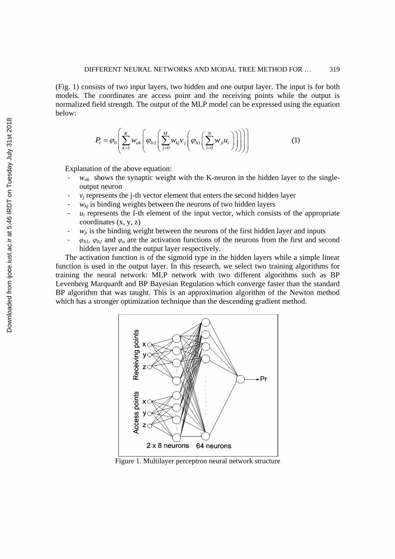
(Fig. 1) consists of two input layers, two hidden and one output layer. The input is for both

models. The coordinates are access point and the receiving points while the output is

normalized field strength. The output of the MLP model can be expressed using the equation

below:

0 2 11 0 0

(1)K M N

r j ji iok h kj hk j i

P w w v w u

Explanation of the above equation:

- wok shows the synaptic weight with the K-neuron in the hidden layer to the single-

output neuron

- vj represents the j-th vector element that enters the second hidden layer

- wkj is binding weights between the neurons of two hidden layers

- ui represents the I-th element of the input vector, which consists of the appropriate

coordinates (x, y, z)

- wji is the binding weight between the neurons of the first hidden layer and inputs

- φh1, φh2 and φo are the activation functions of the neurons from the first and second

hidden layer and the output layer respectively.

The activation function is of the sigmoid type in the hidden layers while a simple linear

function is used in the output layer. In this research, we select two training algorithms for

training the neural network: MLP network with two different algorithms such as BP

Levenberg Marquardt and BP Bayesian Regulation which converge faster than the standard

BP algorithm that was taught. This is an approximation algorithm of the Newton method

which has a stronger optimization technique than the descending gradient method.

Figure 1. Multilayer perceptron neural network structure

Dow

nloa

ded

from

ijoc

e.iu

st.a

c.ir

at 5

:46

IRD

T o

n T

uesd

ay J

uly

31st

201

8

H. Harandizadeh, M. M. Toufigh and V. Toufigh 320

Figure 2. RBF neural network structure

The RBF neural network (Fig. 2) contains an input layer, a hidden layer, and a neuron in

the output layer. The inputs are represented by the coordinates of the access point and the

receiving points. The hidden layer conducts the convert and transfer on data from the input

space to the hidden space. The linear output layer creates the field strength for the proper

input coordinates. The output of the RBF neural network is computed as below:

21 1

( , ) (2)M M

r i i i i i ii i

P w u c w u c

Where u is the input vector (coordinates of the access point and receiving points), i is a

function of the set of all positive real numbers, ||. || shows that Euclidean distance and wi

represents the weights in the output layer, M denotes the number of neurons in hidden layer

and ci is as the RBF centers in the output vector space. The i function is a Gaussian

multivariable function which is defined by the below equation:

2 2

1

2( , ) (3)i

i

u c

iu c e

The parameter determines the width of radial basis function and is commonly known

as the expansion parameter. In our case, the expansion parameter of 0.775 was used.

Normally, the value of 0.5 is used for the expansion parameter, but for this higher value, we

have a better agreement between the measurement value and the simulated data.

A set of 70 samples of measured data was used for training purposes, while the remaining

30 samples were used for testing and simulation purposes. The network training steps

consistently regulate the free network parameters (and weights synaptic) based on the mean

square error of the predicted values and the measured field strength for a set of random

training samples.

Dow

nloa

ded

from

ijoc

e.iu

st.a

c.ir

at 5

:46

IRD

T o

n T

uesd

ay J

uly

31st

201

8

DIFFERENT NEURAL NETWORKS AND MODAL TREE METHOD FOR …

321

2 2

1 1

1 1( ) ( ) (4)

N N

i i ii i

mse e t aN N

Here, ti and ai are the target output and actual output values respectively. When the error

between the output of the network and the desired output is minimized, the training process

is ended. After the training process, the neural network can be used for testing over the test

data.

The main goal of network training is not only to achieve the minimum amount of errors

for the training data set, but also the network should be able to work well with data that is

not used in the training process. This generalization characteristic is very important in the

practical application of the neural model for prediction in environments for which

measurement data is not available. The network generalization feature depends on the

training samples and training algorithm.

4.2 Concepts model tree algorithm

The model tree (MT) is a data-based technique for dealing with continuous class issues

which provides a structured data representation and precise linear fit of classes [13]. Also, it

is a kind of decision tree that has the ability to predict numeric values with linear regression

in leaves and to categorize the data according to their similarity and then matching them

with local regression equations, thus helping to reduce the model error. Quinlan and Wang

and Witten described these popular techniques [9].

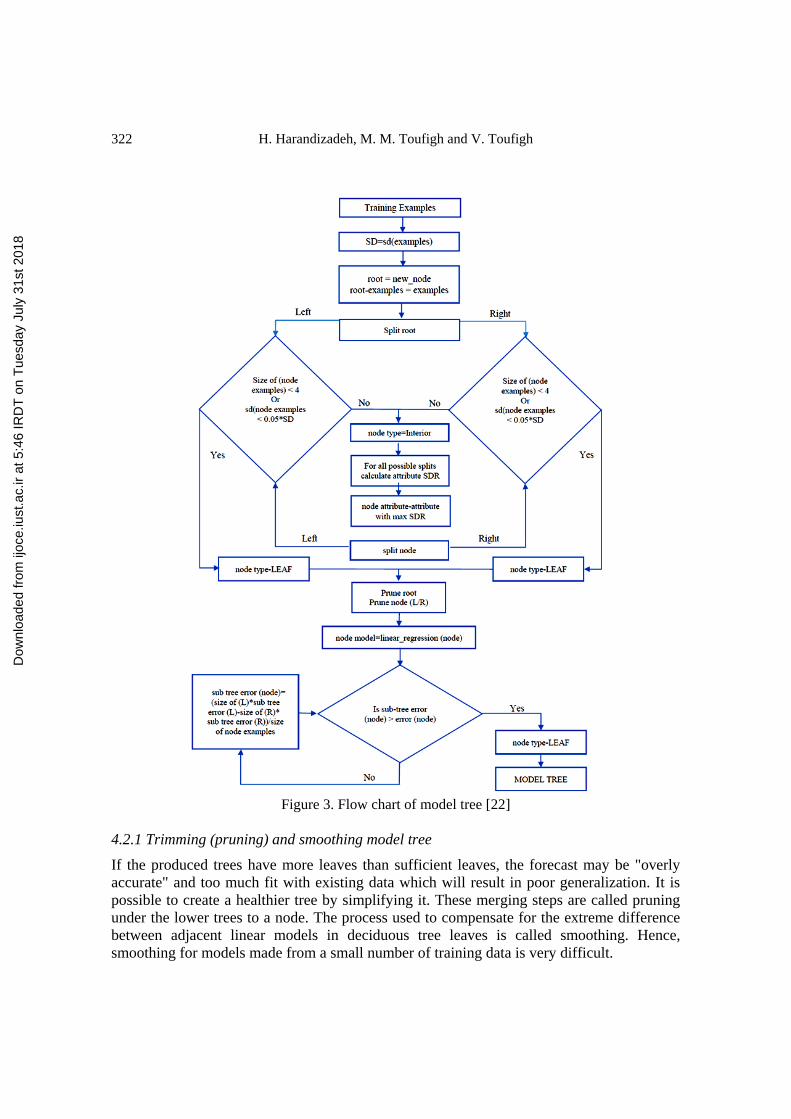
The flowchart of the basic stages of the MT algorithm is shown in Fig. 3, [22]. Initially,

the diagram divides the space of the parameter into sub spaces, then generates a linear

regression model for each sub space. The diagram uses information theory to divide the data

and helps to fit a suitable model. During the formulation of the model, each division section

follows the idea of integrity and combination of the decision tree from several models.

Finally, the flowchart uses intelligent computing techniques for possible solutions for each

model. The main advantages of tree models than regression trees are: (a) Model trees are

much smaller than regression trees; (b) The decision-making power is clear; and (c)

Regression functions typically do not include many variables. Computational requirements

for model trees grow rapidly with dimensions. Hundreds of features are included in the

calculations that help to provide better formulas. Tree-based models develop with the

division and failure method. Standard deviation reduction (SDR) is the main criterion for

choosing a model that is given by the following equation:

( ) ( ) (5)i

i

i

TSDR sd T sd T

T

In which T represents a set of samples that reaches the node; Ti denotes the subset of

samples that result from / * from a potential set (for example, the sets that result from the

division of the node based on the selected attribute) and SD (.) represents the standard

deviation.

Dow

nloa

ded

from

ijoc

e.iu

st.a

c.ir

at 5

:46

IRD

T o

n T

uesd

ay J

uly

31st

201

8

H. Harandizadeh, M. M. Toufigh and V. Toufigh 322

Figure 3. Flow chart of model tree [22]

4.2.1 Trimming (pruning) and smoothing model tree

If the produced trees have more leaves than sufficient leaves, the forecast may be "overly

accurate" and too much fit with existing data which will result in poor generalization. It is

possible to create a healthier tree by simplifying it. These merging steps are called pruning

under the lower trees to a node. The process used to compensate for the extreme difference

between adjacent linear models in deciduous tree leaves is called smoothing. Hence,

smoothing for models made from a small number of training data is very difficult.

Dow

nloa

ded

from

ijoc

e.iu

st.a

c.ir

at 5

:46

IRD

T o

n T

uesd

ay J

uly

31st

201

8

DIFFERENT NEURAL NETWORKS AND MODAL TREE METHOD FOR …

323

5. RESULTS AND DISCUSSION

During the modeling process, the chosen training data set was presented and applied in order

to train the considered learning algorithm to radial basis type neural networks (RBF) and the

multi-layer perceptron neural networks (feedforward MLP). The purpose of training neural

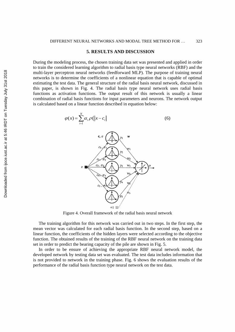
networks is to determine the coefficients of a nonlinear equation that is capable of optimal

estimating the test data. The general structure of the radial basis neural network, discussed in

this paper, is shown in Fig. 4. The radial basis type neural network uses radial basis

functions as activation functions. The output result of this network is usually a linear

combination of radial basis functions for input parameters and neurons. The network output

is calculated based on a linear function described in equation below:

1

( ) ( (6)N

i i

i

x x c

Figure 4. Overall framework of the radial basis neural network

The training algorithm for this network was carried out in two steps. In the first step, the

mean vector was calculated for each radial basis function. In the second step, based on a

linear function, the coefficients of the hidden layers were selected according to the objective

function. The obtained results of the training of the RBF neural network on the training data

set in order to predict the bearing capacity of the pile are shown in Fig. 5.

In order to be ensure of achieving the appropriate RBF neural network model, the

developed network by testing data set was evaluated. The test data includes information that

is not provided to network in the training phase. Fig. 6 shows the evaluation results of the

performance of the radial basis function type neural network on the test data.

Dow

nloa

ded

from

ijoc

e.iu

st.a

c.ir

at 5

:46

IRD

T o

n T

uesd

ay J

uly

31st

201

8

H. Harandizadeh, M. M. Toufigh and V. Toufigh 324

Figure 5. (a) shows the RBF neural network performance based on the training data provided to

the RBF neural network (b) shows the regression coefficient calculated based on the training

data provided to the RBF neural network (c) indicates the error variation in the performance of

the investigating network (d) shows the diagram of the error histogram

Figure 6. (a) indicates the RBF neural network performance based on the test data set provided

to the RBF neural network (b) shows the regression coefficient calculated based on the test data

set provided to the RBF neural network (c) indicates the error variation in the performance of the

investigating network (d) displays the diagram of the error histogram

a

)

b

)

)

)

d

)

)

c

)

)

a

)

b

)

)

)

d

)

)

c

)

)

Dow

nloa

ded

from

ijoc

e.iu

st.a

c.ir

at 5

:46

IRD

T o

n T

uesd

ay J

uly

31st

201

8

DIFFERENT NEURAL NETWORKS AND MODAL TREE METHOD FOR …

325

In order to evaluate the accuracy of the predicted results with the desired target values

and the accuracy of the various used methods, the RBF neural network model was compared

with the Multilayer Perceptron Neural Network (MLP) model based on the Levenberg

Marquardt (LM) and Bayesian Regulation (BR) learning algorithms and also with tree

model (MD). Artificial neural network learning quality evaluation in both training and

testing process was obtained by checking general statistical indices such as Root Mean

Square Error (RMSE) and Mean Absolute Percentage Error (MAPE) values and Correlation

Coefficients.

1

1100% (7)

Ni i

i i

A FMAPE

N A

2

1

1(8)

N

i i

i

RMSE A FN

where N is number of predictions, Ai and Fi are predicted values and actual values

respectively. MAPE is one of the criteria of the error percentage that are popular and one of

the most widely used standards without units. The results of this evaluation for the training

dataset and testing dataset are shown in Table 3 and Table 4 respectively for different

applied methods in this study.

Table 3: Results of the evaluation in training stage for various methods

Correlation RMSE MAPE Methods

0.99875 456.55 14.95 RBF

0.93819 2994.47 22.08 MLP_LM

0.99077 1171.4806 34.04 MLP_BR

0.94102 2602.14 30.23 MODEL TREE

Table 4: Results of evaluation in testing stage for various methods

Correlation RMSE MAPE Methods

0.9892 1430.06 24.49 RBF

0.93032 4837.52 32.06 MLP_LM

0.9849 1647.05 39.35 MLP_BR

0.97395 4248.23 50.61 MODEL TREE

As it can be seen, most of the networks have a high correlation coefficient. However, the

radial basis neural network (RBF) is the highest amount of correlation coefficients.

Compared to ANNs, RBF network is a better answer. Training dataset and testing dataset

have been assigned to values of R = 0.99875, RMSE = 456.55, R = 0.9892 and RMSE =

1430.06 respectively. The other networks which despite the high correlation coefficient,

have a high error in training and testing of their network. The most common networks such

as MLP with simpler structure will significantly decrease network error in case of

eliminating some input parameters and even separation of adhesive soil and granular ones.

Dow

nloa

ded

from

ijoc

e.iu

st.a

c.ir

at 5

:46

IRD

T o

n T

uesd

ay J

uly

31st

201

8

H. Harandizadeh, M. M. Toufigh and V. Toufigh 326

However, with many input parameters, RBF has considered more effective artificial neural

network system to approximate the ultimate bearing capacity of the single piles. Correlation

coefficient charts of mentioned methods together with proposed RBF neural network has

been shown in Fig. 7.

Figure 7. (a) Radial Basis Function Type Neural Network (b) Multilayer Perceptron Neural

Network with Levenberg-Marquardt Backpropagation Training Algorithm (c) Multilayer

Perceptron Neural Network with Bayesian Regulation Backpropagation Training Algorithm (d)

Model Tree Algorithm

6. CONCLUSION

In this research, various neural networks have been developed to calculate and predict the

ultimate axial bearing capacity of single piles on a database collected from existing papers

consisting of 100 prefabricated concrete and steel piles that were presented at the time of the

publication of this study. Always by increasing the training process of neural networks, it is

not expected that the developed network will show a lower error in its output estimation

because the investigating network may be over-trained and learned only training data and

does not respond to not provided test data to the network. In general, in this study, we

concluded that the radial basis neural network (RBF) yielded a response approximately close

Dow

nloa

ded

from

ijoc

e.iu

st.a

c.ir

at 5

:46

IRD

T o

n T

uesd

ay J

uly

31st

201

8

DIFFERENT NEURAL NETWORKS AND MODAL TREE METHOD FOR …

327

to the target value and achieves results with less than 10% of the mean absolute error for the

test data set compared to other used methods. With providing the required information in

order to present to developed neural network and training of the neural network using the

used algorithms, It was concluded that the use of trained neural network techniques was

much simpler than the numerical and empirical methods used to estimate and analyze the

ultimate bearing capacity of piles. It was observed that multi-layer perceptron neural

network error is high due to the number of input data but by decreasing the number of

network input parameters and changing the structure of the investigating network, we can

reduce the error of multilayer perceptron neural networks. However, due to the number of

input parameters (Table 2) and the results of various methods used in this study, it was

determined that the radial basis type neural network has better performance and efficiency

than the methods used to estimate the bearing capacity of the piles with approximation close

to target values.

REFERENCES

1. Goh AT. Empirical design in geotechnics using neural networks, Geotech 1995; 45(4):

709-14.

2. Goh ATC. Pile driving records reanalyzed using neural networks, J Geotech Eng 1996;

122(6): 492-5.

3. Lee IM, Lee JH, Prediction of pile bearing capacity using artificial neural networks,

Comput Geotech 1996; 18(3): 189-200.

4. Teh C, Wong KS, Goh AT, Jaritngam S. Prediction of pile capacity using neural

networks, J Comput Civil Eng 1997; 11(2): 129-38.

5. Kiefa MA. General regression neural networks for driven piles in cohesionless soils, J

Geotech Geoenvironm Eng 1998; 124(12): 1177-85.

6. Hanna AM, Morcous G, Helmy M. Efficiency of pile groups installed in cohesionless

soil using artificial neural networks, Canad Geotech J 2004; 41(6): 1241-9.

7. Shahin MA, Jaksa MB, Maier HR. Recent advances and future challenges for artificial

neural systems in geotechnical engineering applications, Adv Artific Neural Syst 2009;

2009: 5.

8. Najafzadeh M, Barani GA. Comparison of group method of data handling based genetic

programming and back propagation systems to predict scour depth around bridge piers,

Scientia Iranica 2011; 18(6): 1207-13.

9. Najafzadeh M, Laucelli DB, Zahiri A. Application of model tree and evolutionary

polynomial regression for evaluation of sediment transport in pipes, KSCE J Civ Eng

2017; 21(5): 1956–63.

10. Kordjezi A. pooyanejad F. Predicting the bearing capacity of piles using support vector

machine based on CPT data, 2013, Mashhad, Iran.

11. Maizir H, Kassim KA. Neural network application in prediction of axial bearing capacity

of driven piles, in Proceedings of the International MultiConference of Engineers and

Computer Scientists, IMECS, Hong Kong, 2013.

12. McVay MC, Klammler H, Tran K. Pile/Shaft Designs Using Artificial Neural Networks

(ie, Genetic Programming) with Spatial Variability Considerations, 2014.

Dow

nloa

ded

from

ijoc

e.iu

st.a

c.ir

at 5

:46

IRD

T o

n T

uesd

ay J

uly

31st

201

8

H. Harandizadeh, M. M. Toufigh and V. Toufigh 328

13. Najafzadeh M, Barani GA, Hessami-Kermani MR. Group method of data handling to

predict scour depth around vertical piles under regular waves, Scientia Iranica 2013;

20(3): 406-13.

14. Najafzadeh M, Barani GA, Hessami-Kermani MR. Evaluation of GMDH networks for

prediction of local scour depth at bridge abutments in coarse sediments with thinly

armored beds, Ocean Eng 2015; 104, 387-96.

15. Kaveh A, Fazel-Dehkordi D, Servati H. Prediction of moment-rotation characteristic for

saddle-like connections using FEM and BP neural networks, In: International

Conference on Engineering Computational Technology 2000; pp. 15–24.

16. Kaveh A, Raeisi Dehkordi M. Neural networks for the analysis and design of domes, Int

J Sp Struct 2003; 18(3): 181–93.

17. Kaveh A, Iranmanesh A. Comparative study of backpropagation and improved

counterpropagation neural nets in structural analysis and optimization, Int J Sp Struct

1998; 13(4): 177–85.

18. Kaveh A, Servati H. Design of double layer grids using backpropagation neural

networks. Comput Struct 2001; 79(17): 1561-8.

19. Kaveh A, Elmieh R, Servati H. Prediction of moment-rotation characteristic for semi-

rigid connections using BP neural networks, 2001.

20. Kaveh A, Raeisi DM. Application of artificial neural networks for predicting the

displacements of domes under wind loading, 2007.

21. Milad F, Kamal T, Nader H, Erman OE. New method for predicting the ultimate bearing

capacity of driven piles by using Flap number, KSCE J Civ Eng 2015; 19(3): 611–20.

22. Janga Reddy M, Ghimire BNS. Use of model tree and gene expression programming to

predict the suspended sediment Load in rivers, J Intell Syst 2009; 18(3): 211–27.

Available from: http://www.scopus.com/inward/record.url?eid=2-s2.0-71549155647

&partnerID=40&md5=85626306e79226bb9e7380cb8ea745af.

Dow

nloa

ded

from

ijoc

e.iu

st.a

c.ir

at 5

:46

IRD

T o

n T

uesd

ay J

uly

31st

201

8