Diel vertical migration of zooplankton in the Northeast Atlantic

Journal of Plankton Research Vol.18 no.2 pp.163-184,1996

Diel vertical migration of zooplankton in the Northeast Atlantic

Karen J.HeywoodSchool of Environmental Sciences, University of East Anglia, Norwich NR4 7TJ,UK

Abstract. Acoustic Doppler current profiler (ADCP) data collected during August-September 1991reveal the diel migration of zooplankton in the northeast Atlantic (50-60°N, 10-40°W). Volumescattering strength has been calculated, from which the speed and depth of migrations have been stud-ied. There are usually at least two layers displaying nocturnal migration, one spending the day at depthsof 300-400 m and the other at depths of 50-100 m. Reverse migrations are also found to be a commonoccurrence in the region studied. Usually, a surface layer begins to descend at dusk as soon as theupward migrating layer arrives in surface waters. Vertical velocity measured from the ADCP providesthe first detailed direct measurements of the swimming speeds of the populations in situ, which aregenerally between 2 and 6 cm s~'. Migrating animals within layers do not move in unison; the animals atthe leading edge are moving back towards the centre of the layer.

Introduction

Diel vertical migration (DVM) is observed for most species and orders of zoo-plankton, and has long been studied in the laboratory and in situ (see, for example,the review by Forward, 1988). The most common pattern is of ascent to the near-surface layers at dusk, and descent to a deeper layer at dawn, the intervening hoursbeing spent at a relatively constant depth ('nocturnal migration'). A less commonbehaviour exhibits a slow descent following arrival at the surface at dusk, and asubsequent second ascent to the surface towards the end of the night, prior to thedawn descent ('twilight migration'). Other species or stages undergo 'reversemigration', whereby the zooplankton ascend at dawn and descend at dusk. In hisreview of zooplankton behaviour, Haney (1988) comments that although reversemigration is generally believed to be less common, there is little quantitative infor-mation on the frequency of each type of migration. Unless otherwise stated, DVMwill here be assumed to refer to nocturnal migration.

DVM is generally believed to be the result of a compromise between the need tofeed and the need to avoid predation (although other reasons have been suggested,such as the avoidance of damaging UV light; Haney, 1988). Under circumstancesof limited food availability, there is evidence that migration does not take place(Wishner et al., 1988). Light is believed to be the dominant controlling factor, itseffects may include some or all of (i) initiating the ascent or descent, (ii) determin-ing the speed of migration and (iii) constraining the maximum depth attained.

Enright (1977) observed larger upward migration speeds for copepods than hadpreviously been seen (0.8-2.5 cm S"1). but such values have been supported bymore recent observations. For example, Wiebe et al. (1992) estimated swimmingspeeds of 1-6 cm s*1 for copepods and euphausiids. Individual swimming speedsobserved in the laboratory tend to be high (e.g. up to 10 cm s~' for Euphausiapacifica; Torres and Childress, 1983), whereas those for populations observed inthe field are typically an order of magnitude smaller (e.g. 2 cm S"1 for Euphausia

© Oxford University Press 163

Dow

nloaded from https://academ

ic.oup.com/plankt/article-abstract/18/2/163/1521171 by guest on 17 N

ovember 2018

KJ.Heywood

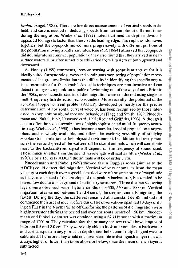
krohni; Angel, 1985). There are few direct measurements of vertical speeds in thefield, and care is needed in deducing speeds from net samples at different timesduring the migration. Wiebe et al. (1992) noted that median depth individualsappeared to migrate faster than those at the leading edge. The euphausiids movedtogether, but the copepods moved more progressively with different portions ofthe population moving at different rates. Roe etal. (1984) observed that copepodsdid not migrate as compact populations; they also found that they arrived in near-surface waters at or after sunset. Speeds varied from 1 to 4 cm s~l both upward anddownward.

As Haney (1988) comments, 'remote sensing with sonar is attractive for it isideally suited for synoptic surveys and continuous monitoring of population move-ments ... The greatest limitation is the difficulty in identifying the specific organ-isms responsible for the signals'. Acoustic techniques are non-invasive and candetect the larger zooplankton capable of swimming out of the way of nets. Prior tothe 1980s, most acoustic studies of diel migration were conducted using single ormulti-frequency fish detection echo sounders. More recently, the potential of theacoustic Doppler current profiler (ADCP), developed primarily for the precisedetermination of horizontal current velocity, has been recognized by those inter-ested in zooplankton abundance and behaviour (Flagg and Smith, 1989; Pluedde-mann and Pinkel, 1989; Heywood etal., 1991; Roe and Griffiths, 1993). Although itcannot offer the size determination of highly sophisticated multi-frequency acous-tics (e.g. Wiebe et al., 1990), it has become a standard tool of physical oceanogra-phers and is widely available, and offers the exciting possibility of studyingzooplankton in relation to their physical environment. In addition, it directly mea-sures the vertical speed of the scatterers. The size of animals which will contributemost to the backscattered signal will depend on the frequency of sound used.Those much smaller than the sound wavelength will scatter little (Wiebe et al.,1990). For a 153 kHz ADCP, the animals will be of order 1 cm.

Plueddemann and Pinkel (1989) showed that a Doppler sonar (similar to theADCP) could detect diel migration. Vertical velocity anomalies from the meanvelocity at each depth over a specified period were of the same order of magnitudeas the vertical speed of the envelope of the peak in backscatter, but tended to bebiased low due to a background of stationary scatterers. Three distinct scatteringlayers were observed, with daytime depths of —300, 560 and 1000 m. Verticalmigration rates varied between 1 and 4 cm s1, the deepest animals migrating thefastest. During the day, the scatterers remained at a constant depth and did notcommence their ascent much before dusk. The observations spanned 13 days drift-ing on FLIP in the North Pacific off California; the patterns of diel migration werehighly persistent during the period and over horizontal scales of ~50 km. Pluedde-mann and Pinkel's data set was obtained using a 67 kHz sonar with a maximumrange of 1200 m. They calculate that the primary scatterers will have lengths ofbetween 0.5 and 2.0 cm. They were only able to look at anomalies in backscatterand vertical speed at any particular depth since their sonar's output signal was notcalibrated. Therefore, they would not have been able to distinguish a layer that wasalways higher or lower than those above or below, since the mean of each layer issubtracted.

164

Dow



ovember 2018

Diel vertical migration of zooplankton

Smith et al. (1989) used an uncalibrated 307 kHz ADCP (scattering primarilyfrom animals of size 0.5 cm or larger) to study zooplankton patchiness, and esti-mated vertical migration rates of 5-8 cm s1 during ascent and of 3-4 cm s~' duringdescent from the peaks of backscatter. This difference between upward and down-ward speed suggested that this population may use gravity to sink rather than swimactively, as proposed by Rudjakov (1970). Most other studies find the migrationsto be symmetrical (e.g. Plueddemann and Pinkel, 1989; Batchelder et al., 1995).Fischer and Visbeck (1993) used moored ADCPs (153 kHz) to study D VM over a 1year period in the Greenland Sea, highlighting the exciting possibilities of zoo-plankton studies under ice. Vertical velocity and relative backscattered energywere determined every 30 min. Strong seasonal variations were observed, maxi-mum migration being observed in February-April and September-October. Thedaytime resting depth was shallower during the winter, with zooplankton migrat-ing only 100 m compared to 350 m in the strongest migration periods. No migrationwas observed during May-July when daylight is nearly continuous. Vertical speedswere small (1-2 cm s"1), with upward motion commencing immediately after sunsetand downward migration finishing before dawn. Neither of these studies was ableto determine absolute backscatter since output signal strength was unknown.More recently, there have been further quantitative comparisons between back-scatter determinations from ADCP and abundance measurements from a compre-hensive net survey [Zhou et al. (1994) in the Southern Ocean and Batchelder et al.(1995) in the North Atlantic]. Batchelder et a/.'s (1995) study was in a similar areaof the North Atlantic to that discussed in this paper, but took place ~3 monthsearlier during the spring bloom, and was a more localized survey.

In this paper, ADCP data collected during a cruise in the North Atlantic (Figure1) are used to investigate the diel migration of scattering layers. The data cover anarea some 2000 x 1000 km, where a variety of physical conditions were encoun-tered, and show many examples of DVM at both dawn and dusk. All the datadiscussed were recorded off the continental shelf in regions of water depths of1000-4000 m. Of particular interest are direct measurements of the migrationvelocities made by the ADCP and their relationship to the vertical layermovement.

Data collection

In 1991 (1 August-4 September), an oceanographic survey (Figure 1) of the NorthAtlantic subpolar gyre was undertaken from RRS 'Charles Darwin' (Gould, 1992).Ninety-six full-depth CTD stations were completed, and continuous observationswere taken using ADCP and a solar irradiance meter. Unfortunately, poorweather conditions were encountered during the cruise, which degraded the qual-ity of the ADCP data—in particular, the noise was increased and the depth pen-etration decreased. The ADCP recorded backscattered signal strength from eachof the four acoustic beams every 2 min. Vertical resolution was chosen to be 8 m;maximum range was —400 m.

165

Dow



ovember 2018

50°N

45°N50°W 40°W 30°W 20°W 10°W

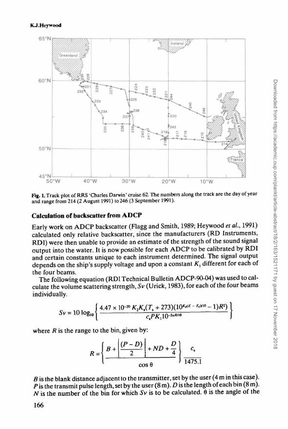
Fig. L Track plot of RRS 'Charles Darwin' cruise 62. The numbers along the track are the day of yearand range from 214 (2 August 1991) to 246 (3 September 1991).

Calculation of backscatter from ADCP

Early work on ADCP backscatter (Flagg and Smith, 1989; Heywood et al., 1991)calculated only relative backscatter, since the manufacturers (RD Instruments,RDI) were then unable to provide an estimate of the strength of the sound signaloutput into the water. It is now possible for each ADCP to be calibrated by RDIand certain constants unique to each instrument determined. The signal outputdepends on the ship's supply voltage and upon a constant K, different for each ofthe four beams.

The following equation (RDI Technical Bulletin ADCP-90-04) was used to cal-culate the volume scattering strength, Sv (Urick, 1983), for each of the four beamsindividually.

= 10 log14.47 x KH° K2K,(TX + 273)(10*<<£

Iwhere R is the range to the bin, given by:

(P-D)B +

cose 1475.1

B is the blank distance adjacent to the transmitter, set by the user (4 m in this case).P is the transmit pulse length, set by the user (8 m). D is the length of each bin (8 m).JV is the number of the bin for which Sv is to be calculated. 0 is the angle of the

166

Dow



ovember 2018


transducer beams to the vertical (30°). c, is the speed of sound, calculated fromsurface temperature and salinity for each profile. K2 is the system noise factormeasured by RDI during calibration, specific to each beam and each ADCP. Kt is aconstant depending on the frequency of the ADCP used. For a 153 kHz ADCP, it is4.17 x 105. Tx is the temperature (°C) of the transducer, recorded internally by theADCP. Kc converts from 'counts' into decibels. This parameter (dB per count) is afunction of the temperature of the system electronics, Tc, which was loggedthroughout the cruise.

. c (7e + 273)

E is the parameter logged as AGC (acoustic gain control) by the ADCP DASsoftware, and is in fact echo intensity in 'counts'. The software records the intensityof the last ping in each 2 min ensemble. A different value of E is obtained for eachbeam. E, is the noise value (counts) for that beam under the particular environ-mental conditions when the profile was obtained (see the discussion below).

a, b and c are constants for the ADCP used; for a ship-mounted system with anominal supply voltage of 220 V, values are 0.699,4.27 and 37.14, respectively. Kic

is a parameter measured by RDI during calibration, specific to each beam and eachADCP. V, is the supply voltage to the ADCP, checked regularly during the cruise(~240 V). a is the sound absorption coefficient (dB nr1). It is a function of tem-perature, salinity and sound frequency (Urick, 1983). The determination of a isdiscussed below.

These equations were used to calculate Sv during the entire cruise, except whenthe ship was in shallow water (<400 m). Arithmetic averages of the values for thefour beams were calculated and will be the data discussed henceforth. Plots of Svfor each of the four beams individually were found to show the same features,although they are more noisy. The diagrams of Sv have been used to calculate theaverage speed of upward or downward layer motion during each migration, bytracking the maximum in backscattered signal intensity. Note that the ADCP can-not detect the presence of scatterers in the upper 10 m due to the depth at which it ismounted in the ship (5 m) and the depth blanked off (4 m).

Sound absorption coefficient, a

The absorption of sound in the sea has been studied experimentally and empiricalrelationships derived considering the contributions due to pure water, boric acidand magnesium sulphate (Urick, 1983). The expressions used here are those due toFrancois and Garrison (1982), who fitted a large global data set to expressionsincluding depth, salinity, temperature, sound frequency and pH. A value of pH of

167

Dow



ovember 2018

KJ.Heywood

8.0 has been assumed and the ADCP frequency is 153 kHz. The remaining datawere extracted from the CTD station data. The sound absorption coefficient wastherefore allowed to vary spatially—significant variations are seen over the area ofthe North Atlantic discussed here (0.048-0.055 dB nr1). In addition, a was calcu-lated as a function of depth (typically varying from 0.05 near surface to 0.04 dB nr1

at 400 m), and an average value calculated for the depth range through which thesound will have travelled to and from the scattering depth.

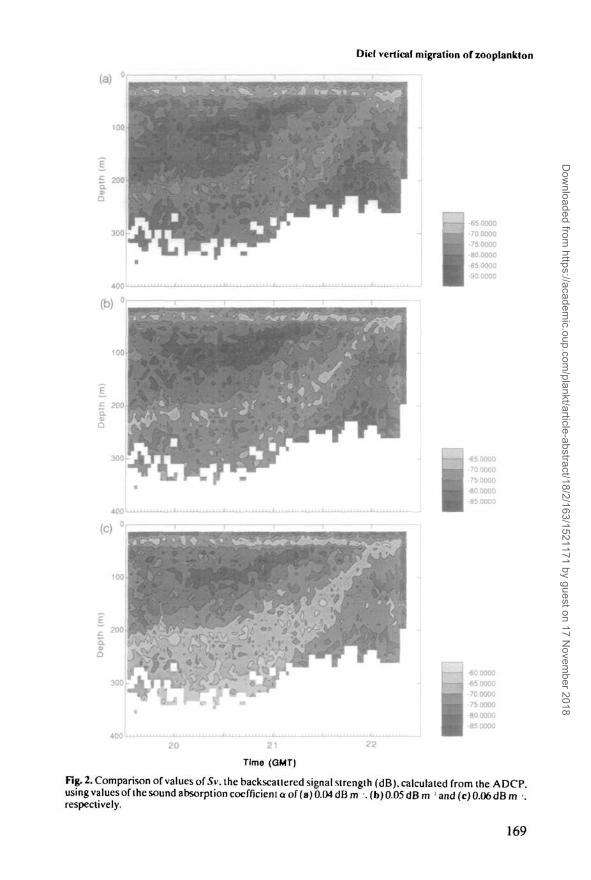
Figure 2 shows the effect of three different values of a, 0.04,0.05 and 0.06 dB nr \constant with depth. This particular example of an upward migration at dusk willbe discussed later; it is shown in Figure 5 with Sv calculated using the value of adeduced from in situ CTD measurements. Here we consider only the influence ofvaring a. With the smallest sound absorption assumed (Figure 2a), backscatteredintensities calculated further from the ADCP are decreased, while if a large soundabsorption is assumed, the formula for 5v predicts a greater density of scatterers atdepth. Notice that in Figure 2a the ascending layer appears to intensify, while inFigure 2c the scattering layer thins as it rises; an artefact of the different soundabsorption. The actual value of a used in Figure 5a is closest to Figure 2b, 0.05 dBnr1, which clearly comes closest to conserving the total amount of backscatteringin the water column and is likely to be the most realistic.

Data quality control

Some care must be exercised in choosing ADCP data for analysis. Problems havepreviously been encountered in calculating backscatter using the ADCP on theRRS 'Charles Darwin' (Heywood etal., 1991) since there is a large flow noise whenthe ship is steaming. Some other installations in other ships (e.g. Batchelder et al.,1995) do not suffer this problem, in which case steaming data may be used withmore confidence. Here the noise, Er, is defined as the backscatter in the lowest bin(number 64), which is well after the point at which the ratio of signal plus noise tonoise tends to one. Some calibrations were carried out in port and in the middle ofthe cruise in deep water, to determine the noise. This procedure is detailed in RDITechnical Bulletin ADCP-90-04. It was found that the noise level for each of thefour beams was substantially different, as expected, and that the noise level whenthe ship was on station was constant throughout the cruise. This value agreed withthe value obtained in port and during the calibration procedures. A 'noise floor'was chosen for each beam (13,13, 23 and 29 counts for beams 1-4, respectively).When processing the data, any profile was rejected where the noise was more than10 counts greater than this floor. In addition, backscatter was set to absent in anyparticular bin if the signal strength was <5 counts greater than the noise, En or if thepercentage of good pings was <5%. This eliminates data points where the signal tonoise ratio is very low. Since data were only considered when the noise value waslow, and this occurred when the ship was on station or steaming slowly, only 13 ofthe possible 63 dawns or dusks during the cruise (2 August-3 September) werestudied. Of these, seven have been chosen to represent the typical range of charac-teristics of scattering layers encountered during the cruise. All the data shown hereare from periods when the ship was maintaining position over the CTD for a goodwire angle.

168

Dow



ovember 2018

Diet vertical migration of zooplankton

400

Time (GMT)

-65 0000•70 0000•75000080 0000

•85.0000-90 0000

I -650000-70.000075 0000

•80 0000•85 0000

Fig. 2. Comparison of values of Sv. the backscatlered signal strength (dB). calculated from the ADCP.using valuesofthesoundabsorptioncoefficientaof(a)0.04dBm .(b)0.05dBm ' and (c) 0.06 dBm •.respectively.

169

Dow



ovember 2018

KJ.Heywood

ADCP vertical velocity and numerical simulation

Although principally intended to measure the horizontal components of velocity,the ADCP also calculates and records the vertical component. It measures thespeed of the scatterers rather than the water itself. Usually the scatterers areassumed to be advected passively with the water. In the case of horizontal veloc-ities, the swimming speed of the plankton is negligible in comparison to the watermovement [except under exceptional circumstances; see, for example, Wilson andFiring (1992)]. For vertical velocities, the water upwelling or downwelling is usu-ally small under general oceanic conditions, except during events such as internalwaves. This paper considers vertical velocity during the periods of diel migration,and claims that the vertical swimming of the zooplankton is directly measured bythe ADCP.

When the ship is steaming, values of vertical velocity are very erratic and not tobe believed. Therefore, the same screening has been applied to the vertical vel-ocity as was applied to the backscatter data. Other authors (e.g. Roe and Griffiths,1993) determine the vertical velocity anomaly at each depth by subtracting themean over a long period or distance, but this approach has not been found necess-ary here (probably because periods of fast steaming are excluded by the stringentnoise criterion).

To test the validity of the vertical speeds observed by the ADCP, a numericalsimulation was undertaken. This models the distribution of scatterers as a functionof depth and time. The scatterers are moved vertically between bins in the modelaccording to the vertical speeds measured by the ADCP, assumed to represent theswimming of the animals. Figure 3 illustrates the scenario envisaged and definesthe variables of the model. Bin number n has a vertical thickness of AZ (here 8 m)and an initial amount of scatterers zoo(n). After time At (here 120 s), the newamount of scatterers zoo' (n) is calculated using the following equation:

, . , , . w(n).A/.zoo(«) w(n + l).Af.zoo(n + 1)zoo' (n) = zoo(«) - A Z + - i A Z

The observed ADCP vertical velocities w(n) and w(n + 1) are strictly in the centreof the bin, but the error involved in assuming it to be valid at the boundariesbetween bins is negligible. If one or both of the vertical velocities is downward,then the equation is adapted to transport scatterers out of the upper bin into thelower one.

The model was initialized using the observed volume scattering strength Sv atthe beginning of the simulated time period in each 8 m vertical bin from the nearsurface to 400 m. There is no spin-up time before the model runs shown in sub-sequent diagrams. The procedure was to run the model forward in time, producinga new depth distribution every 2 min, for comparison with the observed scatterers.Note that, since Sv is logarithmic, it was necessary to take antilogs before adding orsubtracting animals from each 8 m bin, and then convert back to decibels at the endof the time step. Total numbers were conserved by allowing no vertical flux at thesurface or at 400 m.

170

Dow



ovember 2018

Diel vertical migration of zooplanlrton

w(n)

zoo (n) AZ

I zoo (n+1)

Fig. 3. Schematic diagram of the numerical simulation procedure and variables.

To allow a simple quantitative comparison between the simulated and observedvalues of Sv, the root-mean-square (rms) difference between the two values wascalculated for each simulated period, normalized by the observed value of Sv. Thisquantity, designated Q, is calculated using the following equation, where k is thenumber of bins in depth and time where valid values of the observed and simulatedscattering field are available.

* / exp(Sv(simulated)) - exp(5v(observed)) Vi I I

exp(5v(observed)) /

Again this had to be calculated on the non-logarithmic values, hence the calcu-lation of the antilogs. A larger value for this indicates that the simulated backscat-tering field is substantially different from that observed, whereas a smaller valueindicates that the simulation is reasonable. For the examples shown here, valuesfor Q range from 1.0 x 1CH dB for a good simulation to 1.9 x l(h3 dB for a poorsimulation.

Results

Day 216 (4 August; 52°N, 1TW)

The dusk migration of three separate scattering layers can be seen in the contouredbackscattered signal intensity (Figure 4a). All times displayed on figures are GMT,not local time. Lighter shades denote larger backscattered intensities, thus greaterdensities of zooplankton. The shallowest layer has spent the daylight hours near 100m and rises slowly (with an average speed of 0.8 cm S"1) to arrive in the upper 50 m at21:00. It follows fairly closely the 0.2 W nr2 isolume, calculated from the surfacesolar radiation assuming a simple two-exponential decay in class II waters. Twodeeper layers are revealed: one apparently rising from ~250 m and one movingrapidly from a deeper depth; these arrive near the surface at about 21:30 and forma large area of plankton in the upper 50 m during the night. The deeper layers donot follow isolumes. The rapid upward migration starts at about 20:30, which coinci-des with the onset of total darkness. In the vertical speed diagram (Figure 4b),lighter shades denote upward motion and dark shades downward motion. The

171

Dow



ovember 2018

KJ.Heywood

400 » I -70.000075.0000

-80.0000•850000-90.0000

Time (GMT)

172

Dow



ovember 2018


speeds indicated for the deepest layer, which peak at 4 cm s~\ are somewhatsmaller than that determined from the signal intensity (Figure 4a), 6 cm s-'.

The simulation (Figure 4c) shows a layer (again denoted by lighter shades, indi-cating larger numbers of animals) beginning to migrate upwards from —300 m at21:00, as measured by the backscatter (Figure 4a), but it cannot distinguish the twodeeper layers. The rapid rise at about 21:30 is not adequately reproduced, presum-ably because the ADCP vertical velocities are too small. The simulation parameterQ for this period is 1.3 x 10~3 dB. The ADCP vertical speeds are likely to be biasedlow by non-migratory scatterers in the ensonified volume. The near-surfacescattering layer (50-100 m) is also revealed by the model, and indeed the verticalvelocities suggest that it may be this layer which is descending to 200 m (reversemigration) at the same time as the larger layer is migrating upwards.

Day 218 (6 August; 52°N, 2(TW)

At dusk on day 218 (Figure 5a), a distinct layer is seen migrating towards the sur-face containing some scatterers from 230 m and another population from deeperthan 300 m. The vertical speed (Figure 5b) shows that the upper part of the scatter-ing layer is moving downwards, while the lower part moves upwards. Upwardspeeds are greater than downward, as one would expect since the layer as a wholemigrates upwards. Notice also that the layer thins and becomes more concentratedas it rises. A thin surface layer remains at ~30 m throughout; the particles in thelow scattering region below this are moving upwards to join this layer.

The vertical velocities are too small for the model to adequately predict thecomplete ascent at dusk (Figure 6c). However the beginning of the ascent is simu-lated and the difference Q between Figure 5a and c was calculated at 1.5 x 10~3 dB.The vertical velocities (Figure 6b) show a large downward motion at about 22:00,again suggesting reverse migration co-existing, and this prevents the model fromcompleting the upward motion of the main scattering layer.

Day 220 (8 August; 56°TV, 20°W)

Day 220 shows the clearest and most compact layer migrating downwards at dawn(Figure 6). Its thickness is 30-40 m. It also has the highest backscatter of any layerobserved; in places over -60 dB compared to background values of less than -80dB. The layer migrates from night-time levels of ~30 m to below 300 m; later thatday, there was an indication of a layer at 350 m. There was no significant shallowerlayer during the day here. The vertical speed (Figure 6b) does not show a distinctregion of downward migration, rather a diffuse area with peak downward speedsof 2-3 cm s"1. The peak of the backscatter also shows a downward speed of thatmagnitude: 2.7 cm s1. The migration is simulated reasonably (Figure 6c), with avalue of Q of 1.4 x lCh3 dB. The migration starts at least 1 hour before there is anyincrease in solar radiation detected by the solarimeter. It is considerably fasterthan could be accommodated by following isolumes.

Fig. 4. Diel migration at dusk, day 216. Times marked are in GMT. (a) Sv, the backscattered signalstrength (dB), calculated from the ADCP. Blank areas indicate where the data do not satisfy the qualitycriteria discussed in the text. Scattering layers are marked by arrows, (b) Vertical velocity measured byADCP. (c) Numerical simulations of vertical migration using observed vertical velocities. The modelwas initialized at the beginning of the period shown (in this case, 19:30).

173

Dow



ovember 2018

300

400

(0 \

400

Time (GMT\

Fig. 5. Diel migration at dusk, day 218. Otherwise as Figure 4.

| -70 0000

75 0000

80 0000

•85 0000

174

Dow



ovember 2018


400

Time (GMT)


ieooooo65 0O00

70.0000

-75.0000

-80 0000

-85 0000

90 0000

I70.0000

75.0000

80.0000

85.0000

90.0000

175

Dow



ovember 2018

KJ.Heywood

Day 239 (27 August; 53°N, 2TW)

Figure 7, showing dawn on day 239, displays a diffuse downward movement of themain scattering layer, which gets noticeably more dense as it descends. The verticalspeeds show a distinct boundary between upward and downward moving scatter-ers. The maximum speed, up to 4 cm s1, coincides with the maximum backscatter.The scattering layer indicates a vertical migration rate of 3 cm s~', very much inagreement with the speed directly measured. The migration commenced at least 1h before first light was detected by the solarimeter. Notice also the thin (—10 mthick) scattering layer at ~50 m during daylight.

The migration is well simulated (Figure 7c), for both the scattering layer movingdown to 300 m, and the thin layer at 50 m depth. The rms difference Q is calculatedtobel.3xlO-3dB.

Day 240 (28 August; 53°N, 25°W)

Reverse migration is seen clearly on day 240 (Figure 8). The most pronouncedlayer rises at dusk from deeper than 300 m to form a night-time layer at —40 m.Simultaneously a second, thinner layer, which has spent the day at —40 m, de-scends to around 200 m. Because the two layers cannot be clearly distinguished asthey cross, migration speeds estimated from the movement of the peak scatteringmay be erroneous. Figure 8b shows that the scatterers near the surface at 21:30 arepart of the downward migration rather than the upward one. Both the ascendingand descending layers have speeds of the order of 4 cm s~'. The vertical speed(Figure 8b) shows both the upward and downward migrations. The upward mov-ing layer has vertical speeds of 2-4 cm s~l, while the downward moving layer showsspeeds in excess of 4 cm s"1. The reverse migration appears to be triggered either bythe arrival of the other scattering layer, or by sunset. These data were collectedvery close to the Polar Front associated with the North Atlantic Current.

The model can barely cope with such a complex situation (Figure 8c), where onelayer is undergoing nocturnal migration and another layer of similar size is show-ing reverse migration. Such a structure would probably not be revealed by a netstudy, and interpretation of the scattering data without the vertical velocity datawould be open to question. The model emphasizes the reverse migration, since thevertical speeds are larger, and accurately predicts the rate and depth of descent.The difference parameter Q is found to be 1.7 x 10~3 dB, a relatively large valuedespite the apparent agreement 'by eye'. This is probably due to the scatterer-freeregion which develops in the model; possibly in the real data scatterers are enteringthe modelled zone from above the depths measured by the ADCP.

Day 24J (29 August; 53°N, 23°W)

Day 241 shows dusk migrations (Figure 9) between ~30 and 350 m which again areunrelated to isolume depths. A reverse migration is indicated just after dusk, whichfalls at 20:20. The upward migration is interesting since two layers are involved. Ashallower one moves upwards more gradually from —300 m, while a thinner layeris moving upwards from some deeper level more rapidly. The vertical speed plot(Figure 9b) shows the movement of these two layers, the upper one showing

176

Dow



ovember 2018


(a)

7 8Time (GMT


177

Dow



ovember 2018

KJ.Heywood

23


178

i4 0000

2 0000

ooooo-2 0000

4 0000

Dow



ovember 2018


speeds of ~2 cm s~', the lower one between 2 and 4 cm s~'. The distribution ofscatterers during the night appears to be more diffuse than usual, with a broadlayer remaining between 150 and 200 m. Again the reverse migration seems to betriggered either by the arrival of competitors (or predators) or by sunset. The simu-lated distribution (Figure 9c) reveals this complexity and some of the featuresobserved in the scattering data are reproduced: the main layer leaving 300 m tomigrate upwards, a further layer appearing at a greater depth and the reversemigration commencing at 20:30. The simulation is a poor one, showing the largestvalue of Q, 1.9 x 10"3 dB.

Day 246 (3 September; 55°N, 1CPW)

The final diel migration was seen at dawn on day 246 (Figure 10). Two distinctlayers are apparent, both of which start their downward movement at about 05:00,about an hour before any measurable increase in solar radiation. A broad, deeperlayer migrates from —40 to 350 m, fairly rapidly (the speed is not well defined sincethe peak is diffuse, but is between 6 and 9 cm s~'). The vertical speed recorded is 2-4cm s"1. A thin, well-defined upper layer migrates more slowly from a similar depthto ~120 m (speed around 1 cm s"1, while the vertical speed is between 0 and 2 cms"1). The simulation (Figure 10c) exhibits a well-simulated main layer descendingto ~350 m, but the slower downward migration of the near-surface layer is not wellpredicted. For both layers, the rate of descent is too small. This simulation gives thesmallest rms difference between observations and model, Q = 1.0 x 10~3 dB.

Discussion

It is not possible to identify the zooplankton orders or species whose migration hasbeen discussed (there are clearly several). Since they will be of order 1 cm in size,they are likely to be copepods, euphausiids and amphipods. Roe and Griffiths(1993) suggest that the most likely contributors to ADCP backscatter in the north-east Atlantic would be the euphausiid Meganyctiphanes norvegica and the amphi-pod Themisto compressa. Fischer and Visbeck (1993) suggest that their 153 kHzADCP in the Greenland Sea is observing the euphausiid Thyssanoessa longicau-data, but the vertical speeds they observed (of order 1 cm s~') are generally smallerthan those discussed here. Investigations in the Kattegat (quoted by Fischer andVisbeck) also suggested M.norvegica as a likely candidate for fast migrationsobserved by ADCP. A further possibility is that some layers may be small fish, suchas the dominant myctophid Benthosema glaciale (M.Angel, personal communi-cation). Batchelder et al.'s (1995) comprehensive net survey in very much the samearea as discussed here, but 3 months earlier, suggests that Calanus finmarchicusmay be the likely scatterer in this region.

It should be noted that where ADCP data were good enough, diel migrationswere always seen throughout the cruise. They are therefore persistent in both timeand space. All the examples discussed here show nocturnal migration. In addition,reverse migration is revealed to occur in half of the cases discussed—the sameproportion was apparent in days not shown here. It would appear that, at least atdusk, a layer mirrors the nocturnal migration: as soon as the deep layer reaches the

179

Dow



ovember 2018

Dow



ovember 2018


(a)

400

Time (GMT)


181

Dow



ovember 2018

KJ.Heywood

surface, another near-surface layer starts a downward migration. This reversemigration is not coincident with the onset of total darkness or with a maximum inthe rate of change of solar radiation. Rather, it seems to be correlated with thearrival of the other layer, which may be predators or competitors. Such detailedobservations of behaviour are possible only using acoustic methods such as theADCP; furthermore, the vertical velocity information which the ADCP providesis valuable in identifying whether plankton within layers are in fact movingupwards or downwards. The observations at dawn neither support nor rule out theubiquity of reverse migration in this region, since the periods of good data do notstart sufficiently before dawn.

The Polar Front, marking the core of the North Atlantic Current, turns north at~52°N, 20°W, but it is believed that a lesser branch continues to the east to 15°Wwhere it meets waters from the south and turns north. The observations shownhere span both sides of the Polar Front, from warmer, saltier waters to the south-east to cooler, fresher waters to the north and west. Mixed layer depths varied from10-20 m to the east of the Polar Front to 50-60 m to the west of it. Scattering layersobserved throughout the cruise had a tendency during their near-surface period tobe located in the pycnocline, at the peak(s) in stratification just below the mixedlayer. They were usually associated with a decrease in dissolved oxygenconcentration.

ADCP speeds are consistently smaller than those of peak in scattering. Pluedde-mann and Pinkel (1989) also found the Doppler velocities to be biased low, andexplained that this will be due to a background of non-migrating scatterers. Theybelieved the migrators to be a small proportion of the scattering field; as this pro-portion increases, the Doppler velocities will more fairly represent the speed of themigrating animals. Nevertheless, one should be aware that the scattering layeritself can move faster than any of its constituent individuals. The simple simulationof the scattering layers by applying the observed ADCP vertical velocities hasdemonstrated that the Doppler currents are able to provide the necessarymigration speeds. The downward migrations are generally simulated better thanupward ones, suggesting that there may be a small bias in the vertical speedsmeasured by the ADCP.

The layers which migrate only within the upper 100 m do appear to migratefollowing isolumes and their motion may be initiated by changes in the relative rateof change of solar radiation. However, most scattering layers migrate to ~400 m,and these ascend and descend more rapidly than the isolumes. They consistentlypre-empt dawn by ~1 h. It is known that some species may have an internal clockwhich is reset daily. Might it also be possible that some species can detect light atthe UV end of the spectrum, where dawn would appear more than half an hourbefore it would be evident in the visible? Forward (1988) discusses the sensitivityof zooplankton to spectral differences, and most evidence suggests a peak sensi-tivity in the blue-green which penetrates most deeply in ocean waters. No determi-nation of their sensitivity to UV is mentioned. Animals who could react morepromptly to dawn by detecting UV light before dawn is apparent in the visibleband would have an advantage over their competitors. Although some freshwaterfish have been shown to have UV vision, Partridge (1990) concludes that 'the

182

Dow



ovember 2018

Dlel vertical migration of zooptankton

importance of ultra-violet vision in marine fish is speculative'. Adult fish tend notto have lenses that are transparent to UV light, whereas juveniles or larvae do, sohe suggests that by analogy with freshwater fish, sensitivity to UV light is mostlikely to be found in larvae or juveniles living in areas of low levels of Gelbstoff,such as the open ocean of the northeast Atlantic.

The ADCP vertical currents show that the zooplankton like to keep togetherduring upward migrations, the upper animals move down towards the centre of thelayer and during downward migrations the lower animals move upwards intothe layer. The numerical simulation supported the validity of these observationsin the vertical velocities. Wiebe et al. (1992) also observed that the 'median depthindividuals as a whole appeared to migrate faster than their leading edgecounterparts'.

Acknowledgements

I wish to thank Dr John Gould, Principal Scientist of RRS 'Charles Darwin' cruise62. This work was supported by NERC grant GR9/581 and my participation in thecruise by NERC WOCE Special Topic grant GST/02y576. I am grateful to DrMartin Angel (IOSDL) for valuable suggestions and to an anonymous referee forhelpful and constructive criticism.

ReferencesAngel,M.V. (1985) Vertical migrations in the oceanic realm: Possible causes and probable effects. In

Rankin,M.A. (ed.), Migration: Mechanisms and Adaptive Significance. Port Aransas: Mar. ScL Inst.,Contrib. Mar. Sci., 27(SuppL), 45-70.

Batchelder,H.P., VanKeuren J.R., Vaillancourt,R. and Swift£. (1995) Spatial and temporal distri-butions of acoustically estimated zooplankton biomass near the Marine Light-Mixed Layers station(59°30'N, 21°00'W) in the North Atlantic in May 1991. /. Geophys. Res., 100, 6549-6563.

EnrightJ.T. (1977) Copepods in a hurry: sustained high-speed upward migration. LimnoL Oceanogr.,22,118-125.

FischerJ. and Visbeck,M. (1993) Seasonal variation of the daily zooplankton migration in the Green-land Sea. Deep-Sea Res., 40,1547-1557.

Flagg.C.N. and Smith,S.L. (1989) On the use of the acoustic Doppler current profiler to measure zoo-plankton abundance. Deep-Sea Res., 36,455-474.

Forward,R.B. (1988) Diel vertical migration: zooplankton photobiology and behaviour. Oceanogr.Mar. Biol. Annu. Rev., 26, 361-393.

Francois,R.E. and Garrison,G.R. (1982) Sound absorption based on ocean measurements. J. ACOUSLSoc. Am., 72,1879-1890.

Gould.WJ. (1992) RRS Charles Darwin Cruise 62,01 Aug-04 Sep 1991, CONVEX-WOCE ControlVolume AR12. IOSDL Cruise Report No. 230,60 pp.

HaneyJ.F. (1988) Diel patterns of zooplankton behaviour. Bull Mar. Sci., 43,583-603.Heywood,KJ., Scrope-Howe,S. and Barton.E.D. (1991) Estimation of zooplankton abundance from

shipbome ADCP backscatter. Deep-Sea Res., 38,677-691.PartridgeJ.C. (1990) The colour sensitivity and vision of fishes. In Herring^ J., Campbell^A.K., Whit-

fleld JvI.R. and Maddock,L. (eds), Light and Life in the Sea. Cambridge University Press, pp. 167-184.Plueddemann A J- and Pinkel,R. (1989) Characterization of the patterns of diel migration using a Dop-

pler sonar. Deep-Sea Res., 36, 509-530.Roe,H.S_J. and Griffiths,G. (1993) Biological information from an acoustic Doppler current profiler.

Mar. Biol., 115,339-346.RoeJiSJ., Angel,M.V., BadcockJ., Domanski,P., James,P.T., Pugh.P.R. and ThurstonJvl.H. (1984)

The diel migrations and distributions within a mesopelagic community in the North East AtlanticProg. Oceanogr., 13,245-511.

RudjakovJ. A. (1970) The possible causes of diel vertical migrations of planktonic animals. Mar. Biol.,6,98-105.

183

Dow



ovember 2018

KJ.Heywood

Smith J'.E., Ohman.M.D. and Eber,LE. (1989) Analysis of the patterns of distribution of zooplanktonaggregations from an acoustic Doppler current profiler. CalCOFI Rep., 30, 88-103.

TorresJJ. and ChildressJJ. (1983) Relationship of oxygen consumption to swimming speed inEuphausia pacifica. 1. Effects of temperature and pressure. Mar. BioL, 74,79-86.

Urick.R J. (1983) Principles of Underwater Sound. McGraw-Hill, New York, 423 pp.Wiebe.P.H., Greene.C.H., Stanton.T.K. and Burczynski J. (1990) Sound scattering by live zooplankton

and micronekton: empirical studies with a dual-beam acoustical system. J. Acousu Soc. Am., 88,2346-2360.

Wiebe.P.H., Copley,NJ. and Boyd.S.H. (1992) Coarse-scale horizontal patchiness and verticalmigration of zooplankton in Gulf Stream warm-core ring 82-H. Deep-Sea Res., 39(SuppL),S247-S278.

Wilson,C.D. and Firing.E. (1992) Sunrise swimmers bias acoustic Doppler current profiles. Deep-SeaRes., 39,885-892.

WishnerJC., Durbin,E., Durbin^A., Macaulay.M., Winn.H. and Kenney.R. (1988) Copepod patchesand right whales in the Great South Channel off New England. Bull Mar. Sci., 43,825-844.

Zhou.M., Nordhausen,W. and Huntley,M. (1994) ADCP measurements of the distribution and abun-dance of euphausiids near the Antarctic Peninsula in winter. Deep-Sea Res., 41,1425-1445.

Received on November 25, 1994; accepted on October 13, 1995

184

Dow



ovember 2018

Diel vertical migration of zooplankton in the Northeast Atlantic

Documents

Transcript of Diel vertical migration of zooplankton in the Northeast Atlantic