DHI Eutrophication Model 1 – Including Sediment and Benthic Vegetation … · 2017-10-08 · DHI...
54
MIKE 2017 DHI Eutrophication Model 1 – Including Sediment and Benthic Vegetation MIKE ECO Lab Template Scientific Description
Transcript of DHI Eutrophication Model 1 – Including Sediment and Benthic Vegetation … · 2017-10-08 · DHI...

MIKE 2017
DHI Eutrophication Model 1 – Including Sediment and Benthic Vegetation
MIKE ECO Lab Template
Scientific Description

dhi_eutrophication_model_1_sediment_benthic_veg.docx/PSR/MPO/2017-09-13 - © DHI
DHI headquarters
Agern Allé 5
DK-2970 Hørsholm
Denmark
+45 4516 9200 Telephone
+45 4516 9333 Support
+45 4516 9292 Telefax
www.mikepoweredbydhi.com

i
CONTENTS
DHI Eutrophication Model 1 – Including Sediment and Benthic Vegetation MIKE ECO Lab Template Scientific Description
1 Introduction ....................................................................................................................... 1
2 Applications ...................................................................................................................... 3
3 Mathematical Formulations .............................................................................................. 5 3.1 Phytoplankton Carbon (PC) ................................................................................................................. 6 3.2 Phytoplankton Nitrogen (PN) ............................................................................................................. 10 3.3 Phytoplankton Phosphorus (PP) ........................................................................................................ 10 3.4 Chlorophyll-a (CH) ............................................................................................................................. 11 3.5 Zooplankton (ZC) ............................................................................................................................... 12 3.6 Detritus ............................................................................................................................................... 14 3.7 Detritus Carbon (DC) ......................................................................................................................... 15 3.8 Detritus Nitrogen (DN) ........................................................................................................................ 16 3.9 Detritus Phosphorus (DP) .................................................................................................................. 17 3.10 Inorganic Nitrogen (IN) ....................................................................................................................... 18 3.11 Inorganic Phosphorus (IP) ................................................................................................................. 20 3.12 Oxygen (DO) ...................................................................................................................................... 21 3.13 Benthic Vegetation (BC)..................................................................................................................... 23
4 Extended Description of Macroalgae and Rooted Vegetation ..................................... 25 4.1 Macroalgae ........................................................................................................................................ 25 4.2 Rooted Vegetation ............................................................................................................................. 25
5 Extended Sediment Description .................................................................................... 29 5.1 N and P Cycle in the Sediment Module ............................................................................................. 29 5.2 Nitrogen Processes ............................................................................................................................ 31 5.3 Phosphorus Processes ...................................................................................................................... 36 5.4 Differential Equations ......................................................................................................................... 38 5.5 Parameters ......................................................................................................................................... 39
6 Future Developments ..................................................................................................... 41
7 Solution Technique ......................................................................................................... 43
8 Data Requirements ......................................................................................................... 45
9 List of References ........................................................................................................... 47

DHI Eutrophication Model 1 – Including Sediment and Benthic Vegetation
ii MIKE ECO Lab Template - © DHI

Introduction
1
1 Introduction
MIKE ECO Lab is a numerical lab for Ecological Modelling. It is a generic and open tool
for customising aquatic ecosystem models to describe water quality and eutrophication
amongst others. DHI’s expertise and knowhow concerning ecological modelling has been
collected in predefined ecosystem descriptions (MIKE ECO Lab templates) to be loaded
and used in MIKE ECO Lab. So the MIKE ECO Lab templates describe physical,
chemical and biological processes related to environmental problems and water pollution.
The following is a description of the DHI Eutrophication Model 1 including an extended
description of sediment and benthic vegetation.
The template is used in investigations of eutrophication effects and as an instrument in
environmental impact assessments. The eutrophication modelling can be applied in
environmental impact assessments considering:
• Pollution sources such as domestic and industrial sewage and agricultural run-off
• Cooling water outlets from power plants resulting in excess temperatures
• Physical conditions such as sediment loads and change in bed topography affecting
especially the benthic vegetation.
The aim of using eutrophication modelling as an instrument in environmental impact
assessment studies is to obtain, most efficiently in relation to economy and technology,
the optimal solution with regards to ecology and the human environment.
The Eutrophication Model 1 describes nutrient cycling, phytoplankton and zooplankton
growth, growth and distribution of rooted vegetation and macroalgae in addition to
simulating oxygen conditions.
The model results describe the concentrations of phytoplankton, chlorophyll-a,
zooplankton, organic matter (detritus), organic and inorganic nutrients, oxygen and the
area-based biomass of benthic vegetation over time. In addition, a number of derived
variables are stored: primary production, total nitrogen and phosphorus concentrations,
sediment oxygen demand and secchi disc depth.
The Eutrophication Model 1 is integrated with the advection-dispersion module which
describes the physical transport processes at each grid-point covering the area of
interest. Other data required are concentrations at model boundaries, flow and
concentrations from pollution sources, water temperature and irradiance etc.

DHI Eutrophication Model 1 – Including Sediment and Benthic Vegetation
2 MIKE ECO Lab Template - © DHI

Applications
3
2 Applications
The DHI Eutrophication Model 1 template can be applied in a range of environmental
investigations:
• Studies where the effects of alternative nutrient loading scenarios are compared
and/or different waste water treatment strategies are evaluated
• Studies of oxygen depletion
• Studies of the effects of the discharge of cooling water
• Comparisons of the environmental consequences of different construction concepts
for harbours, bridges, etc.
• Evaluation of the environmental consequences of developing new urban and
industrial areas.

DHI Eutrophication Model 1 – Including Sediment and Benthic Vegetation
4 MIKE ECO Lab Template - © DHI

Mathematical Formulations
5
3 Mathematical Formulations
The Eutrophication Model 1 is coupled to the advection modules of DHI hydraulic engines
in order to simulate the simultaneous processes of transport, dispersion and
biological/biochemical processes. The eutrophication model 1 incl. sediment and benthic
vegetation results in a system of 25 differential equations describing the variations for 12
standard state variables and the extended desription of macroalgae and rooted vegetation
includes additional 4 state variables and the extended description of the sediment
includes additional 9 state variables. The first 11 state variables are found in the pelagic
system and are socalled advective state variables. The additional state variables belong
to the benthic system. The benthic vegetation is attached to the sea bed, stones or the
like. It is, therefore, not subject to transport by water movements or to dispersion. The
sediment state variables are not subject to transport either.
The statndard 12 state variables of the Eutrophication Model 1 are:
• Phytoplankton carbon (PC) (gC/m3)
• Phytoplankton nitrogen (PN) (gN/m3)
• Phytoplankton phosphorus (PP) (gP/m3)
• Chlorophyll-a (CH) (g/m3)
• Zooplankton (ZC) (gC/m3)
• Detritus carbon (DC) (gC/m3)
• Detritus nitrogen (DN) (gN/m3)
• Detritus phosphorus (DP) (gP/m3)
• Inorganic nitrogen (IN) (gN/m3)
• Inorganic phosphorus (IP) (gP/m3)
• Dissolved oxygen (DO) (g/m3)
• Benthic vegetation carbon (BC) (gC/m2)
The extended description of the benthic system (macroalgae and rooted vegetation)
includes 4 more state variables:
• Benthic vegetation nitrogen (BN) (gN/m2)
• Benthic vegetation phosphorus (BP) (gP/m2)
• Eelgrass carbon (EC) (gC/m2)
• Eelgrass shoot numbers pr m2 (No/m2)
The extended description of the sediment includes the 9 state variables:
• KDOX, depth of NO3 penetration in sediment (m)
• SIP, Sediment phosphate in pore water (gP/m3)
• SPIM, Sediment P, immobile fraction (gP/m2)
• FESP, Sediment iron absorped P (gP/m2)
• SOP, Sediment organic P (gP/m2)
• SON, Sediment organic NN (gN/m2)
• SNH, Sediment ammonia NH4-N in pore water (gN/m3)
• SNO3, NO3-N in Surface sediment pore water (gN/m3)
• SNIM, Sediment N, immobile fraction (gN/m2)
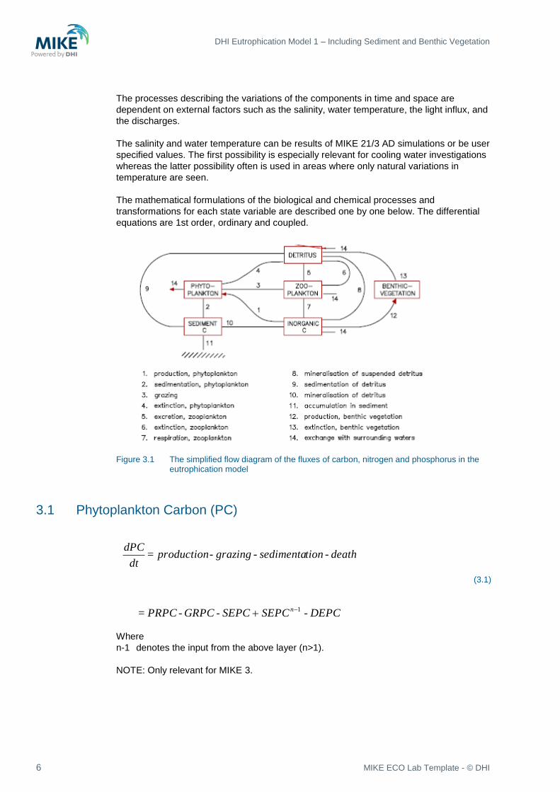
The processes and transfer of carbon, nitrogen and phosphorus in the Eutrophication
model system is illustrated in Figure 3.1. Also included in the model is an oxygen balance.
DHI Eutrophication Model 1 – Including Sediment and Benthic Vegetation
6 MIKE ECO Lab Template - © DHI
The processes describing the variations of the components in time and space are
dependent on external factors such as the salinity, water temperature, the light influx, and
the discharges.
The salinity and water temperature can be results of MIKE 21/3 AD simulations or be user
specified values. The first possibility is especially relevant for cooling water investigations
whereas the latter possibility often is used in areas where only natural variations in
temperature are seen.
The mathematical formulations of the biological and chemical processes and
transformations for each state variable are described one by one below. The differential
equations are 1st order, ordinary and coupled.
Figure 3.1 The simplified flow diagram of the fluxes of carbon, nitrogen and phosphorus in the
eutrophication model
3.1 Phytoplankton Carbon (PC)
DEPC - SEPC SEPC- GRPC - PRPC =
death - tion sedimenta- grazing - production = dt
dPC
n 1
(3.1)
Where
n-1 denotes the input from the above layer (n>1).
NOTE: Only relevant for MIKE 3.

Mathematical Formulations
7
Figure 3.2 Interaction of temperature with light and nutrients. Top left: Photosynthetic rate of
Cladophora albida under different levels of light intensity and temperatures in estuarine water. Adapted from Gordon et al. (1980). Right: Mean (± standard deviation) division rates during exponential phase of growth in Talassiosira fluviatilis at three temperatures and daylengths (18, 21, and 6 hrs). Adapted from Hobson (1974). © Canadian Journal of Aquatic and Fisheries Sciences. Bottom left: Maximum photosynthetic rate (Pmax) of natural phytoplankton of Tokyo Bay under varying phosphate concentrations and temperatures. Adapted from Ichimura (1967). (from: Valiela, 1984)
Production (PRPC)
The net production of phytoplankton is light, temperature and nutrient dependent.
RD FAC P)(N,F (T)F F(I) = PRPC 11 (3.2)
Where
μ = maximum growth coefficient at 20oC (d-1)
FAC = correction factor for dark reaction
RD = relative day length
Light function
IKI
IKIIKIIF
1
/)( (3.3)
Where
IK = . i(T-20) = light saturation (E/m2/d)

DHI Eutrophication Model 1 – Including Sediment and Benthic Vegetation
8 MIKE ECO Lab Template - © DHI
I = actual irradiance (E/m2/d)
= light saturation level for algae at 20oC (E/m2/d)
i = temperature parameter
T = water temperature (oC)
The irradiance at the surface (in E.m-2.d-1) is integrated analytically over depth until the
depth of the actual layer, given the value of I in the light function. The light function then
determines the relative light saturation level. In this model, the light saturation level may
be made temperature-dependent, reflecting the observation that phytoplankton groups,
such as dinoflagellates, that reach maximum abundance in late summer, have higher light
saturation levels (Figure 3.2; cf. Valiela, 1984). In shallow, low-volume systems, where
there is only a short lag between irradiance level and water temperature, a temperature
dependency may be used to reflect physiological adaptation to ambient light intensity.
Temperature function
20)-(T
g1 = (T)F (3.4)
Where
g = temperature coefficient for growth
Temperature for phytoplankton plays a major role as a covariate with other factors.
Phytoplankton at low temperatures maintain greater concentrations of photosynthetic
pigments, enzymes and carbon (Steemann, Nielsen & Jørgensen, 1968), enabling more
efficient use of light. There are strong interactions between temperature and Max at any
light intensity, with day length and production, and with nutrient uptake. In general, all
rates increase with increasing temperatures and the irradiance level where maximum
photosynthesis is reached is shifted to higher values with increasing temperatures.
Nutrient dependence function
Since phytoplankton growth depends essentially on the size of the internal nutrient pools,
the nutrient-dependent growth limitation F1(N,P) is calculated from the relative saturation
of the internal N and P pools. Droop (1973, 1975) provides a theoretical basis for this
approach which also has been incorporated in a theoretical model by Nyholm (1977) and
in North Sea models by Mommaerts (1978), Tett et al. (1986) and Lancelot & Rousseau
(1987).
)PP-PP/PC+(KC )PP-PP(
)PP-PP+(KC )PP-(PP/PC = F(P)
PP - PN
PN - PN/PC = F(N)
F(P)
1 +
F(N)
1
2 = P)(N,F1
minminmax
minmaxmin
minmax
min
(3.5)

Mathematical Formulations
9
Where
PNmin,PNmax = minimum and maximum internal nitrogen content in algae
(gN/gC), respectively
PPmin,PPmax = minimum and maximum phosphorus content in algae (gP/gC),
respectively
KC = half saturation constant for phosphorus in phytoplankton
(gP/gC)
Death of phytoplankton (DEPC)
Natural mortality of phytoplankton, or autolysis, has been shown to be a significant
phenomenon in the marine ecosystem (Jassby & Goldman, 1974) and this decay of
blooms is partly mineralised in the water column (Lancelot et al., 1987). In this model, the
natural mortality of phytoplankton increases as the internal nutrient pools decrease.
The death rate is assumed to be proportional to the nutritional status of the phytoplankton
PC P)(N,F = DEPC 2d (3.6)
Where
d = death rate under optimal nutrient conditions (d-1)
F2(N,P) = ½.{PNmax/(PN/PC) + PPmax/(PP/PC)}
F2(N,P) is a function with a minimum of 1. and a maximum when PN/PC
and PP/PC ratios are at a minimum. The maximum value of
F2(N,P) depends on the specified PNmia and PPmn coefficients.
The maximum value will typically be around 10.
Sedimentation of phytoplankton (SEPC)
Nutrient-replete phytoplankton is able to adjust its buoyancy and hence, to minimise its
sinking rate. Under conditions of nutrient-stress, with the internal nutrient pools at lower
levels, sinking rates increase (Smayda, 1970, 1971).
At low water depth (h<2 m):
PC P)(N,F = SEPC 2s (3.7)
and at water depth h2 m:
PC P)(N,F /hU = SEPC 2s (3.8)
Where
s = sedimentation rate parameter (d-1)
Us = sedimentation velocity (m/d)
h = water depth (m)
The internal pools of phytoplankton nutrients in this model are state variables, because
their uptake dynamics are decoupled from the phytoplankton carbon assimilation

DHI Eutrophication Model 1 – Including Sediment and Benthic Vegetation
10 MIKE ECO Lab Template - © DHI
dynamics, resulting in time-varying PN/PC and PP/PC ratios. However, the nutrient pools
being internal to the carbon-based phytoplankton, their source and sink terms are
proportional to the corresponding phytoplankton carbon rates.
3.2 Phytoplankton Nitrogen (PN)
The mass balance for phytoplankton nitrogen reads:
DEPN - SEPN SEPN- GRPN - UNPN =
death - tion sedimenta- grazing - uptake = dt
dPN
n 1
(3.9)
Where
n-1 denotes the input from the above layer (n>1).
NOTE: Only relevant for MIKE 3.
The rates are similar to the ones for phytoplankton carbon.
Uptake (UNPN)
A description of the nitrogen uptake from phytoplankton can be found in section about the
inorganic nitrogen.
Grazing (GRPN)
(PN/PC) GRPC = GRPN (3.10)
Sedimentation (SEPN)
(PN/PC) SEPC= SEPN (3.11)
Death (DEPN)
(PN/PC) DEPC = DEPN (3.12)
3.3 Phytoplankton Phosphorus (PP)
The mass balance for phytoplankton phosphorus reads:
DEPPSEPPSEPPGRPPUPPP
death-ndimentatiosegrazinguptakedt
dPP
n
1
(3.13)
Mathematical Formulations
11
Where
n-1 denotes the input from the above layer (n>1).
NOTE: Only relevant for MIKE 3.
The rates are similar to the ones for phytoplankton carbon.
Uptake (UPPP)
A description of the phosphorus uptake from phytoplankton can be found in section about
the inorganic phosphorus.
Grazing (GRPP)
(PP/PC) GRPC = GRPP (3.14)
Sedimentation (SEPP)
(PP/PC) SEPC= SEPP (3.15)
Death
(PP/PC) DEPC = DEPP (3.16)
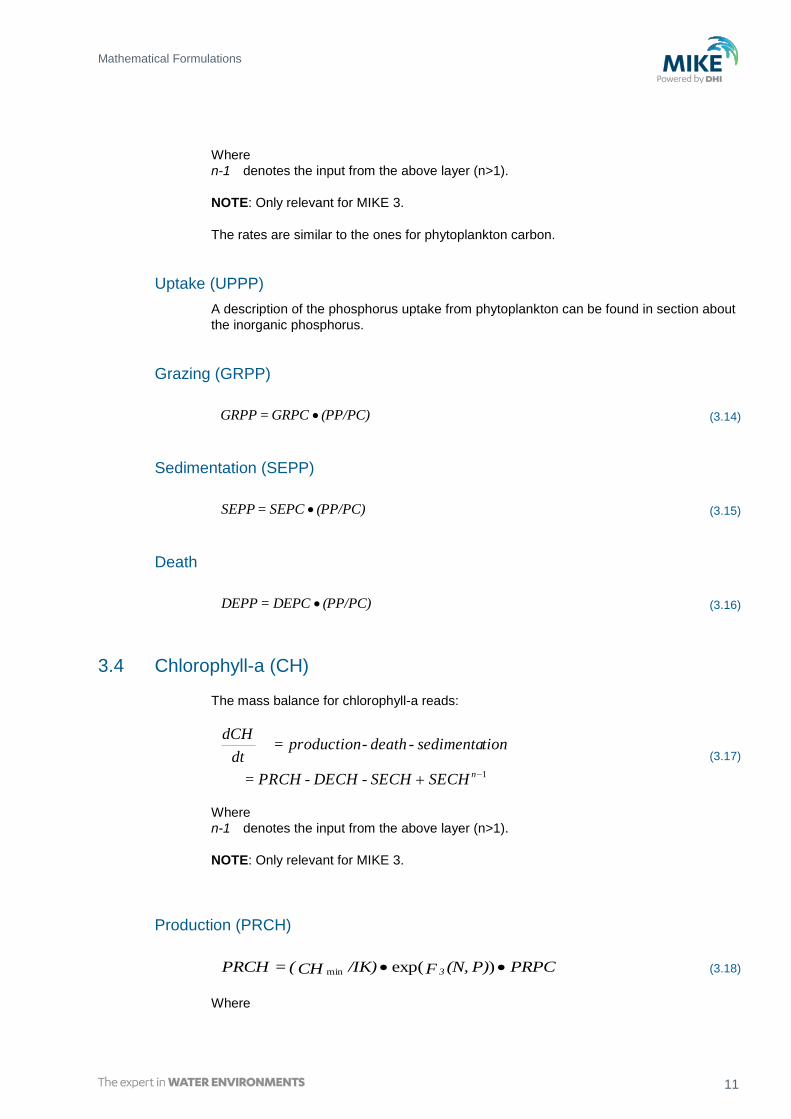
3.4 Chlorophyll-a (CH)
The mass balance for chlorophyll-a reads:
1 nSECH SECH- DECH - PRCH =
tion sedimenta- death - production = dt
dCH
(3.17)
Where
n-1 denotes the input from the above layer (n>1).
NOTE: Only relevant for MIKE 3.
Production (PRCH)
PRPC P)(N,F /IK)CH( = PRCH 3 )exp(min (3.18)
Where
DHI Eutrophication Model 1 – Including Sediment and Benthic Vegetation
12 MIKE ECO Lab Template - © DHI
CHmin = coefficient determining the minimum chlorophyll-a production
(E/m2/d)-1
F3(N) = CHmax . {(PN/PC-PNmin)/(PNmax-PNmin)}
CHmax = coefficient determining the maximum chlorophyll-a production
(n.u.) in the absence of nutrient limitation.
Sedimentation (SECH)
(CH/PC) SEPC= SECH (3.19)
Death (DECH)
(CH/PC) GRPC) + (DEPC = DECH (3.20)
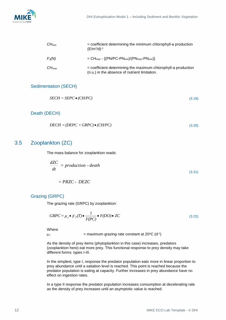
3.5 Zooplankton (ZC)
The mass balance for zooplankton reads:
DEZC - PRZC =
death - production = dt
dZC
(3.21)
Grazing (GRPC)
The grazing rate (GRPC) by zooplankton:
ZC F(DO) F(PC)
1 (T)F = GRPC 2z
(3.22)
Where
z = maximum grazing rate constant at 20oC (d-1)
As the density of prey items (phytoplankton in this case) increases, predators
(zooplankton here) eat more prey. This functional response to prey density may take
different forms: types I-III.
In the simplest, type I, response the predator population eats more in linear proportion to
prey abundance until a satiation level is reached. This point is reached because the
predator population is eating at capacity. Further increases in prey abundance have no
effect on ingestion rates.
In a type II response the predator population increases consumption at decelerating rate
as the density of prey increases until an asymptotic value is reached.

Mathematical Formulations
13
In this model a type III functional response has been formulated (see Valiela, 1984 for a
review of the literature on types of functional response). Type III has a density-dependent
portion where the rate of ingestion accelerates with increasing prey density. At higher
prey densities the type III behaves much like the type II functional response, with the
percentage mortality caused per predator becoming lower at increasing prey density
down to an asymptotic value.
The parameters K1 and K2 determine the onset and the extent of the density-dependent
portion of the functional response.
Temperature function
20)-(T
z2 = (T)F (3.23)
Where
z = temperature coefficient for grazing rate
Phytoplankton dependence function
e + 1 = F(PC) PC)K-K( 21 (3.24)
Where
K1,K2 = factors describing the grazing rate dependence on phytoplankton
biomass (N.U. and m3/g respectively)
Oxygen dependence function
MDO+ DO
DO = F(DO)
2
2
(3.25)
Where
MDO = oxygen concentration indicating depressed grazing rates due to
oxygen depletion
Production (PRZC)
The production is coupled closely to the grazing of phytoplankton:
GRPC V = PRZC C (3.26)
Where
VC = growth efficiency parameter for zooplankton (n.u.)

DHI Eutrophication Model 1 – Including Sediment and Benthic Vegetation
14 MIKE ECO Lab Template - © DHI
Respiration (REZC)
Respiration of zooplankton can be described as proportional to the grazing of
phytoplankton by ignoring basic metabolism, since activity respiration dominates
respiratory processes.
GRPC K = REZC R (3.27)
Where
KR = proportionality constant
Death (DEZC)
Zooplankton mortality has a density-independent term as in Horwood (1974). The density-
dependent term is a closure term, which is necessary in the model because zooplankton
is the highest trophic level explicitly modelled. For a discussion of the closure problem,
see Steele (1976).
The zooplankton decay is proportional to the zooplankton concentration, but at high
densities the dependence is of second order resulting in:
ZC K + ZC K = DEZC 2dd 21 (3.28)
Where
Kd1 = rate constant (d-1) especially important at concentrations below 1
g.m-3.
Kd2 = rate constant important at high concentrations
{d-1.(g/m3)-1}
The zooplankton assimilation efficiency is not 100% resulting in an excretion (EKZC) of
nutrients (C, N and P) being the difference between grazing, production and respiration:
REZC - PRZC - GRPC = EKZC (3.29)
These excretion products are organic material entering the organic matter/detritus pool as
outlined below in the detritus equations.
3.6 Detritus
Detritus is defined in the model as particles of dead organic material in the water. The
detritus pool receives the dead primary producers and excreted material left after grazing.
Sedimentation and mineralisation are the only processes draining the detritus pools.
There are three state variables: detritus carbon, nitrogen and phosphorus.
Mathematical Formulations
15
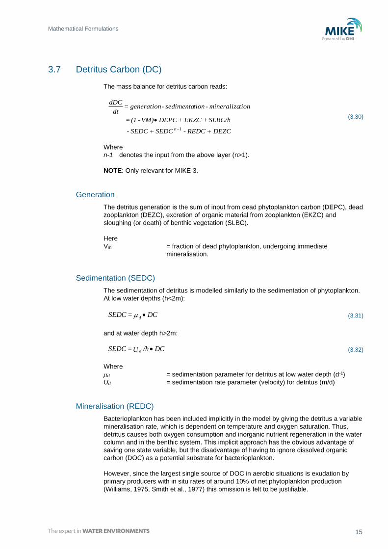
3.7 Detritus Carbon (DC)
The mass balance for detritus carbon reads:
DEZCREDC - SEDC SEDC-
SLBC/h+ EKZC + DEPC VM)-(1 =
tionmineraliza - tion sedimenta- generation = dt
dDC
n
1
(3.30)
Where
n-1 denotes the input from the above layer (n>1).
NOTE: Only relevant for MIKE 3.
Generation
The detritus generation is the sum of input from dead phytoplankton carbon (DEPC), dead
zooplankton (DEZC), excretion of organic material from zooplankton (EKZC) and
sloughing (or death) of benthic vegetation (SLBC).
Here
Vm = fraction of dead phytoplankton, undergoing immediate
mineralisation.
Sedimentation (SEDC)
The sedimentation of detritus is modelled similarly to the sedimentation of phytoplankton.
At low water depths (h<2m):
DC = SEDCd (3.31)
and at water depth h>2m:
DC /hU = SEDC d (3.32)
Where
d = sedimentation parameter for detritus at low water depth (d-1)
Ud = sedimentation rate parameter (velocity) for detritus (m/d)
Mineralisation (REDC)
Bacterioplankton has been included implicitly in the model by giving the detritus a variable
mineralisation rate, which is dependent on temperature and oxygen saturation. Thus,
detritus causes both oxygen consumption and inorganic nutrient regeneration in the water
column and in the benthic system. This implicit approach has the obvious advantage of
saving one state variable, but the disadvantage of having to ignore dissolved organic
carbon (DOC) as a potential substrate for bacterioplankton.
However, since the largest single source of DOC in aerobic situations is exudation by
primary producers with in situ rates of around 10% of net phytoplankton production
(Williams, 1975, Smith et al., 1977) this omission is felt to be justifiable.
DHI Eutrophication Model 1 – Including Sediment and Benthic Vegetation
16 MIKE ECO Lab Template - © DHI
Nutrient regeneration from the benthic system by mineralisation processes is not
dependent on the benthic detritus pool but on the sedimentation rate of pelagic detritus.
Proportionality factors define the permanent loss of nutrients (adsorption, complexation,
burial, denitrification) from the system.
DC (DO)F (T)F = REDC 13m (3.33)
Where
m = maximum mineralisation rate at 20oC (d-1)
F3(T) = D(T-20)
D = temperature coefficient for mineralisation of detritus
F1(DO) = DO2/(DO2 + MDO)
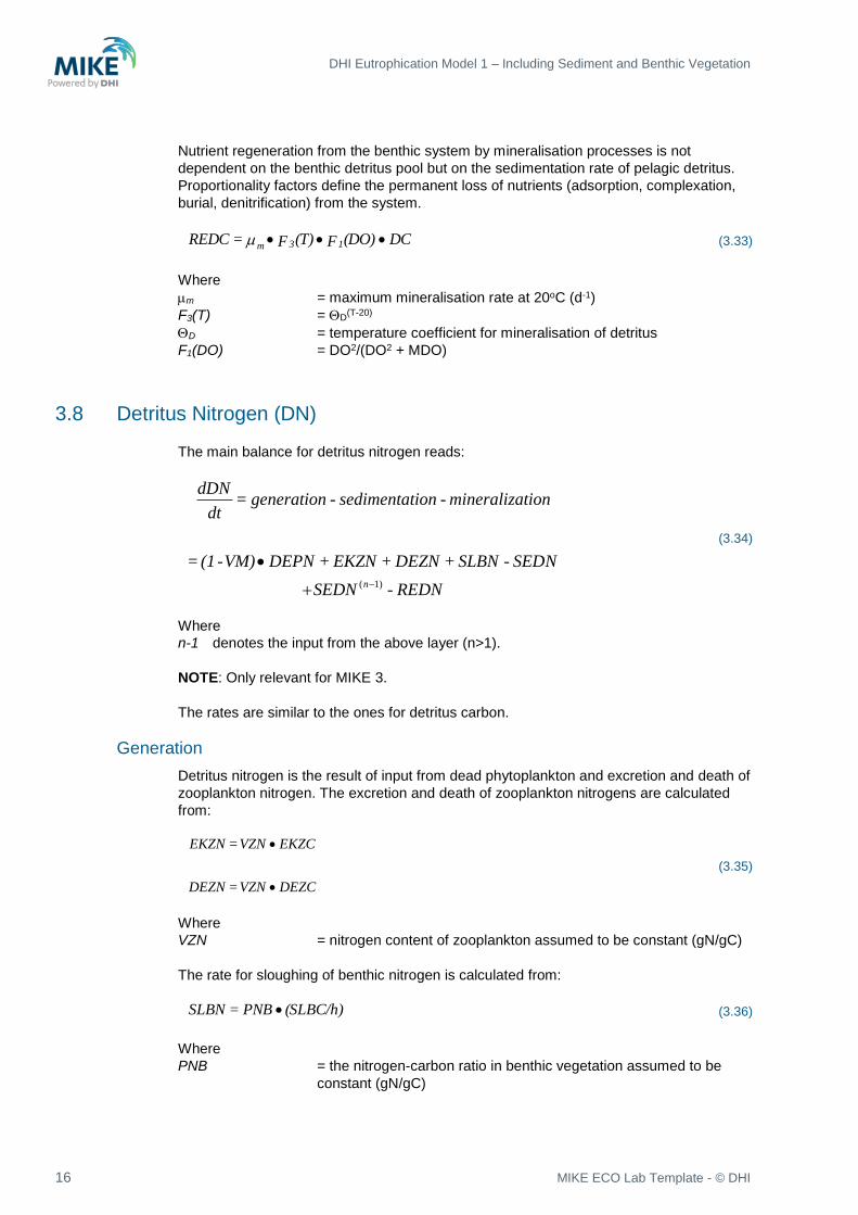
3.8 Detritus Nitrogen (DN)
The main balance for detritus nitrogen reads:
( 1)n
dDN = generation - sedimentation - mineralization
dt
= (1 -VM) DEPN + EKZN + DEZN + SLBN - SEDN
SEDN - REDN
(3.34)
Where
n-1 denotes the input from the above layer (n>1).
NOTE: Only relevant for MIKE 3.
The rates are similar to the ones for detritus carbon.
Generation
Detritus nitrogen is the result of input from dead phytoplankton and excretion and death of
zooplankton nitrogen. The excretion and death of zooplankton nitrogens are calculated
from:
DEZC VZN = DEZN
EKZC VZN = EKZN
(3.35)
Where
VZN = nitrogen content of zooplankton assumed to be constant (gN/gC)
The rate for sloughing of benthic nitrogen is calculated from:
(SLBC/h) PNB = SLBN (3.36)
Where
PNB = the nitrogen-carbon ratio in benthic vegetation assumed to be
constant (gN/gC)

Mathematical Formulations
17
Sedimentation
DN/DC SEDC= SEDN (3.37)
Mineralisation
DN/DC REDC = REDN (3.38)
3.9 Detritus Phosphorus (DP)
The mass balance for detritus phosphorus reads:
( 1)n
dDP = generation - sedimentation - mineralization
dt
= (1 -VM) DEPP + EKZP + DEZP + SLBP - SEDP
SEDP - REDP
(3.39)
Where
n-1 denotes the input from the above layer (n>1).
NOTE: Only relevant for MIKE 3.
The rates for phosphorus are similar to the detritus carbon rates.
Generation
This is the sum of phosphorus from dead phytoplankton, excretion and death of
zooplankton phosphorus and sloughing of benthic vegetation phosphorus.
The excretion and death of zooplankton phosphorus and the sloughing of benthic
phosphorus are expressed as:
(SLBC/h) PPB = SLBP
DEZC VZP = DEZP
EKZC VZP = EKZP
(3.40)
Where
VZP = the constant phosphorus content of zooplankton (gP/gC)
PPB = the constant phosphorus content of benthic vegetation (gP/gC)
DHI Eutrophication Model 1 – Including Sediment and Benthic Vegetation
18 MIKE ECO Lab Template - © DHI
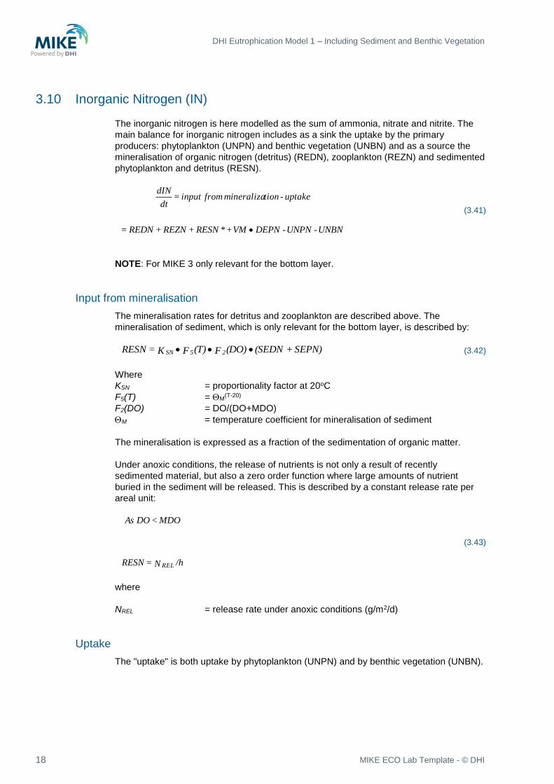
3.10 Inorganic Nitrogen (IN)
The inorganic nitrogen is here modelled as the sum of ammonia, nitrate and nitrite. The
main balance for inorganic nitrogen includes as a sink the uptake by the primary
producers: phytoplankton (UNPN) and benthic vegetation (UNBN) and as a source the
mineralisation of organic nitrogen (detritus) (REDN), zooplankton (REZN) and sedimented
phytoplankton and detritus (RESN).
UNBN - UNPN - DEPN VM + RESN + REZN + REDN =
uptake - tionmineraliza from input = dt
dIN
*
(3.41)
NOTE: For MIKE 3 only relevant for the bottom layer.
Input from mineralisation
The mineralisation rates for detritus and zooplankton are described above. The
mineralisation of sediment, which is only relevant for the bottom layer, is described by:
SEPN)+ (SEDN (DO)F (T)F K = RESN 25SN (3.42)
Where
KSN = proportionality factor at 20oC
F5(T) = M(T-20)
F2(DO) = DO/(DO+MDO)
M = temperature coefficient for mineralisation of sediment
The mineralisation is expressed as a fraction of the sedimentation of organic matter.
Under anoxic conditions, the release of nutrients is not only a result of recently
sedimented material, but also a zero order function where large amounts of nutrient
buried in the sediment will be released. This is described by a constant release rate per
areal unit:
/hN = RESN
MDO< DO As
REL
(3.43)
where
NREL = release rate under anoxic conditions (g/m2/d)
Uptake
The "uptake" is both uptake by phytoplankton (UNPN) and by benthic vegetation (UNBN).

Mathematical Formulations
19
Uptake by phytoplankton (UNPN)
The model for phytoplankton includes modelling of nutrient limited growth determined by
intracellular concentrations. The uptake is then different for limited and non-limited
conditions. Under limiting conditions where PN<PNmax the uptake rate of nitrogen is
chosen from three expressions in the following way:
PN PRPC
supplyexternal + tionMineraliza
PCKPNIN
INV
-
- = UNPN
kn
max
max
min (3.44)
This scheme states that under limiting conditions the uptake is determined either by the
extracellular concentration (IN) or by the release of nutrients by biological and chemical
decomposition processes and external supply. The highest value of these two is chosen.
This shall of course not exceed the uptake as determined by the production and
maximum nitrogen content. The latter is also true for the non-limiting condition where a
choice of the minimum of the following values is made:
PN PRPC
PC KPNIN
IN V
- = UNPN
kn
max
min (3.45)
Where
Vkn = the uptake rate constant for nitrogen (d-1.(mg/l)-1)
KPN = Halfsaturation concentration for N uptake(mg N/l)
Uptake by benthic vegetation (UNBN)
The model for the benthic vegetation does not include a nutrient limited growth as a
function of intracellular concentration but a slightly more simple approach in which the
extracellular nutrient concentration may be growth limiting. The nutrient uptake is then
proportional to the net production.
(PRBC/h) PNB = UNBN (3.46)
Where
PNB = nitrogen to carbon ratio (gN/gC)
PRBC = production of benthic carbon (see later for the benthic vegetation
mass balance)

DHI Eutrophication Model 1 – Including Sediment and Benthic Vegetation
20 MIKE ECO Lab Template - © DHI
The growth limitation function is described together with the production of benthic
vegetation below.
3.11 Inorganic Phosphorus (IP)
The main balance for inorganic phosphorus (e.g. phosphate) reads:
UPBP - UPPP - DEPP VM + RESP + REZP + REDP =
uptake - tionmineraliza from input = dt
dIP
*
(3.47)
NOTE: For MIKE 3 only relevant for the bottom layer.
The rates are very similar to the rates for nitrogen.
Input from mineralisation
The input from mineralisation is the sum of mineralisation of detritus, zooplankton and
phytoplankton phosphorus and the release from the sediment.
Release from the sediment, which is only relevant for the bottom layer, is expressed as:
SEPP)+ (SEDP (DO)F (T)F K = RESP 25SP (3.48)
Where
KSP = proportionality factor at 20oC
The remainder of the terms in this equation have been explained above.
Under anoxic conditions (DO<MDO) a constant release rate is modelled:
/hP = RESP REL (3.49)
Where
PREL = constant release rate (g/m2/d)
Uptake
Uptake by phytoplankton is described similarly to the nitrogen uptake.
Under non-limiting conditions:
PP PRPC
PC KPPIP
IP V
- = UPPP
kp
max
min (3.50)
Mathematical Formulations
21
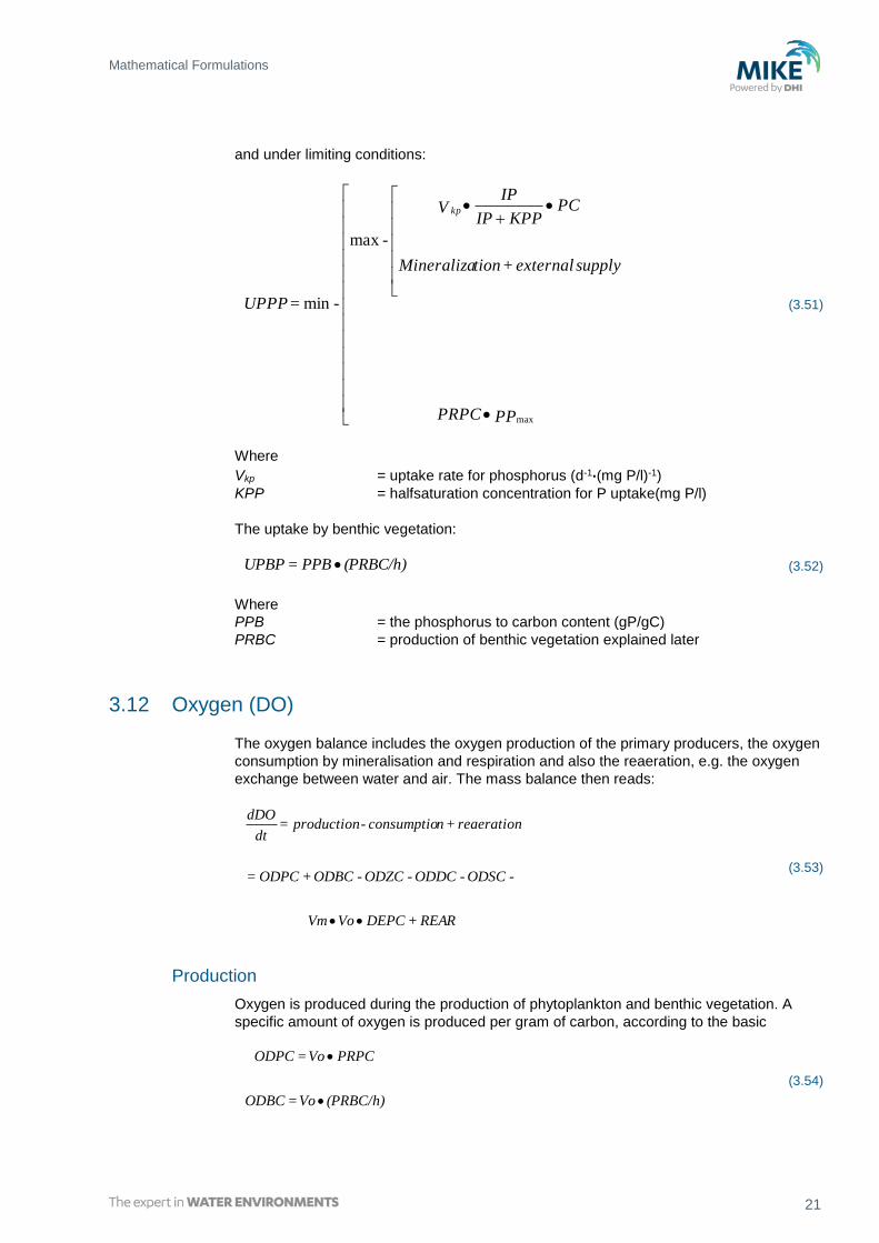
and under limiting conditions:
PP PRPC
supplyexternal + tionMineraliza
PC KPPIP
IP V
-
- = UPPP
kp
max
max
min (3.51)
Where
Vkp = uptake rate for phosphorus (d-1.(mg P/l)-1)
KPP = halfsaturation concentration for P uptake(mg P/l)
The uptake by benthic vegetation:
(PRBC/h) PPB = UPBP (3.52)
Where
PPB = the phosphorus to carbon content (gP/gC)
PRBC = production of benthic vegetation explained later
3.12 Oxygen (DO)
The oxygen balance includes the oxygen production of the primary producers, the oxygen
consumption by mineralisation and respiration and also the reaeration, e.g. the oxygen
exchange between water and air. The mass balance then reads:
REAR + DEPC Vo Vm
- ODSC - ODDC - ODZC - ODBC + ODPC=
reaeration + nconsumptio - production = dt
dDO
(3.53)
Production
Oxygen is produced during the production of phytoplankton and benthic vegetation. A
specific amount of oxygen is produced per gram of carbon, according to the basic
(PRBC/h) Vo = ODBC
PRPC Vo = ODPC
(3.54)
DHI Eutrophication Model 1 – Including Sediment and Benthic Vegetation
22 MIKE ECO Lab Template - © DHI
Where
Vo = oxygen to carbon ratio at production (gO2/gC)
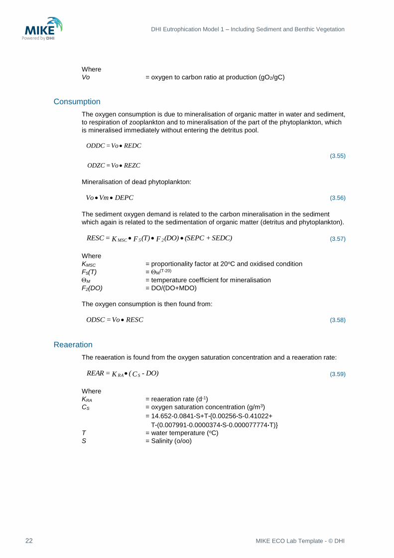
Consumption
The oxygen consumption is due to mineralisation of organic matter in water and sediment,
to respiration of zooplankton and to mineralisation of the part of the phytoplankton, which
is mineralised immediately without entering the detritus pool.
REZC Vo = ODZC
REDC Vo = ODDC
(3.55)
Mineralisation of dead phytoplankton:
DEPC Vm Vo (3.56)
The sediment oxygen demand is related to the carbon mineralisation in the sediment
which again is related to the sedimentation of organic matter (detritus and phytoplankton).
SEDC)+ (SEPC (DO)F (T)F K = RESC 25MSC (3.57)
Where
KMSC = proportionality factor at 20oC and oxidised condition
F5(T) = M(T-20)
M = temperature coefficient for mineralisation
F2(DO) = DO/(DO+MDO)
The oxygen consumption is then found from:
RESC Vo = ODSC (3.58)
Reaeration
The reaeration is found from the oxygen saturation concentration and a reaeration rate:
DO) - C( K = REAR SRA (3.59)
Where
KRA = reaeration rate (d-1)
CS = oxygen saturation concentration (g/m3)
= 14.652-0.0841.S+T.{0.00256.S-0.41022+
T.(0.007991-0.0000374.S-0.000077774.T)}
T = water temperature (oC)
S = Salinity (o/oo)
Mathematical Formulations
23
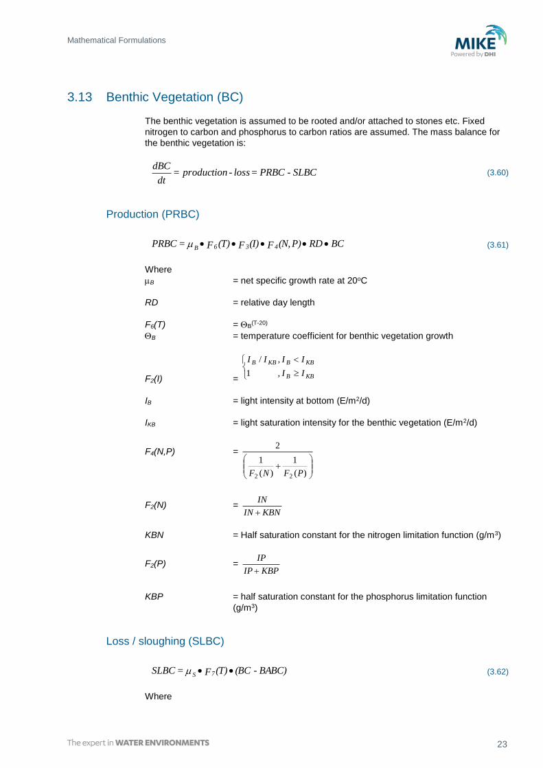
3.13 Benthic Vegetation (BC)
The benthic vegetation is assumed to be rooted and/or attached to stones etc. Fixed
nitrogen to carbon and phosphorus to carbon ratios are assumed. The mass balance for
the benthic vegetation is:
SLBC- PRBC = loss - production = dt
dBC (3.60)
Production (PRBC)
BC RD P)(N,F (I)F (T)F = PRBC 436B (3.61)
Where
B = net specific growth rate at 20oC
RD = relative day length
F6(T) = B(T-20)
B = temperature coefficient for benthic vegetation growth
F2(I) =
KBB
KBBKBB
II
IIII
,1
,/
IB = light intensity at bottom (E/m2/d)
IKB = light saturation intensity for the benthic vegetation (E/m2/d)
F4(N,P) =
)(
1
)(
1
2
22 PFNF
F2(N) = KBNIN
IN
KBN = Half saturation constant for the nitrogen limitation function (g/m3)
F2(P) = KBPIP
IP
KBP = half saturation constant for the phosphorus limitation function
(g/m3)
Loss / sloughing (SLBC)
BABC) - (BC (T)F = SLBC 7S (3.62)
Where

DHI Eutrophication Model 1 – Including Sediment and Benthic Vegetation
24 MIKE ECO Lab Template - © DHI
S = sloughing or loss rate at 20oC (d-1)
F7(T) = S(T-20)
S = temperature coefficient for loss
BABC = minimum area based biomass of benthic vegetation (g/m2)

Extended Description of Macroalgae and Rooted Vegetation
25
4 Extended Description of Macroalgae and Rooted Vegetation
4.1 Macroalgae
The extended description of macroalgae includes three state variables: macroalgae
carbon (BC), -nitrogen (BN) and – phosphorus (BP). The macroalgae submodel consists
of 3 differential equations, one for each state variable. Each equation contains the rates
describing algae production and death.
dBC/dt = production – death= PRBC-DEBC
dBN/dt = uptake of nitrogen – death • BN/BL
dBP/dt = uptake of phosphorus – death • BP/BL
The description of the production of macroalgae C (PRBC) is the same as the standard
EU description of production of benthic vegetation C. The death is dependent on
temperature and a death rate kslm:
BCtetlkslmDEBC temp 20 (4.1)
The nutrient uptake (N and P) of macroalgae is very similar to the description of nutrient
uptake of phytoplankton with a nutrients dependence function
4.2 Rooted Vegetation
The model describes the seasonal variations in the aboveground production and biomass
of rooted vegetation. Two types of growth (production) are included: one is leaf elongation
(i.e. increase in shoot biomass) and the other is development of new shoots. The above
ground biomass is the mean biomass of a shoot times the number of shoots pr m2.
Both young and old shoots, young and large shoots are seen in an eelgrass population at
all times of the year. Nevertheless, small shoots are dominating in winter/spring and large
shoots are dominating in summer/autumn. Assuming the seasonally varying mean
biomass of a shoot to be representative for the size of the shoots in the population is
therefore reasonable.
The net production of one shoot as well as the evolution of new shoots is depending on
external forcing functions as light and temperature. Nutrient limitations of growth are not
accounted for in the model. It is assumed that eelgrass can get sufficient nutrients from
either the water or the sediment
The description of rooted vegetation e.g. eelgrass includes two state variables, mean
biomass of one shoot (EC) and the number of shoots (NNEC).
dEC/dt = production - death =PREC-DEEC
dNNEC/dt =production of shoots–loss off shoots=DNDT-PLOSS
Production of rooted vegetation biomass per shoot is described with the expression
PREC:

DHI Eutrophication Model 1 – Including Sediment and Benthic Vegetation
26 MIKE ECO Lab Template - © DHI
1ftECRDmyiemegrPREC (4.2)
Where
megr = Growth rate
myie = Light function describing the growth dependence on light at the bed
RD = Relative day length
ft1 = Arrhenius temperature expression201 tempteta
teta1 = Temperature coefficient for rooted vegetation growth
Loss of rooted vegetation biomass per shoot is described by the expression DEEC:
ECfhftmedrDEEC 22 (4.3)
Where
medr = Death rate
ft2 = Arrhenius temperature expression:2022 temptetaft
teta = Temperature coefficient for rooted vegetation shoot death
fh2 = Factor for depth dependent death. The factor can be used to
describe death as a result of wave impact at shallow water:
The production of new shoots is described with the expression DNDT:
RDftmyiemngrDNDT 1 (4.4)
Extended Description of Macroalgae and Rooted Vegetation
27
Where
mngr = Growth rate for shoot density
myie = Light function describing the growth dependence on light at the bed.
The light function for shoot production include benthic shading
RD = Relative day length
ft1 = Arrhenius temperature expression201 tempteta
teta1 = the temperature coefficient for rooted vegetation growth
The loss of shoots is described by the expression PLOSS:
NNECklossPLOSS (4.5)
Where
kloss = Loss rate for shoot density

DHI Eutrophication Model 1 – Including Sediment and Benthic Vegetation
28 MIKE ECO Lab Template - © DHI

Extended Sediment Description
29
5 Extended Sediment Description
The Standard Eutrophication model has a simple description of sediment release of
nitrogen and phosphorus which returns a fraction of the settled P to the sediment back
into the water column. This approach has shown sufficient when describing systems with
moderate nutrient loading or with low retention time. However in systems with high
loading and/or high retention time the description has shown to be insufficient.
The sediment module is an add-on module to the standard EU module and therefore uses
the state variables and some of the processes as input. The sediment module is
constructed in a way so it is possible to use in connection with other add on module like
the eelgrass module.
The present description is restricted to the Sediment but may use terms from the
Standard EU description.
5.1 N and P Cycle in the Sediment Module
The state variables and the processes in the sediment model are listed below and
presented in Figure 5.1 and Figure 5.2 for nitrogen and phosphorus respectively.
The nitrogen cycle consists of three state variables and one sink: Organic N in the
sediment (SON), total NH4 (SNH), NO3 (SNO3) and immobile nitrogen (SNIM).
Sedimentation of organic N or flux of NH4 and NO3 across the sediment surface connects
the state variables to plankton N, detritus N and inorganic N in the water. The organic N
in the sediment is mineralised producing NH4, which enters the SNH pool. NH4 in the
sediment may either be exchanged with IN in the water or nitrified to NO3 in the
uppermost layer of the sediment with O2.
The NO3 entering the SNO3 pool may either be denitrified or exchanged with inorganic N
in the water.
The phosphorus cycle in the sediment consist likewise of three state variables and a sink:
leachable organic P, (SOP), PO4-P in pore water (SIP), PO4-P adsorbed to Fe+++ (SPFE)
and immobile P (SIMP).
A fraction of the plankton P and detritus P which settles on the sediment surface is
undergoes decomposition or are eaten by deposit feeders in the sediment before it is
incorporated into the sediment. Some of the P will therefore be turned to PO4 and the rest
will enter the pool of organic P in the sediment. The processes FSPB and RSOP describe
these fluxes of P, see Figure 5.1.
A fraction of the P entering the sediment surface will be buried in deeper sediment layers
chemical bound to apatite (CaCO3) or to refractory organic matter, Jensen/1995/ and
Sundby/1992/. This is described in the model by letting a fraction of the organic P go into
the pool of immobilised P (SIMP).
The pool of leachable organic P (SOP) is degraded to PO4 (process ROPSIP) and
released into the pore water pool of PO4 (SIP). Besides the organic P, the pool of
adsorbed PO4 to oxidised Fe shown to be the most important P component for the P cycle

DHI Eutrophication Model 1 – Including Sediment and Benthic Vegetation
30 MIKE ECO Lab Template - © DHI
in marine coastal sediments, ref. Mortensen /1992/ and Jensen /1995/. Therefore a pool
of PO4 adsorbed to Fe+++ has been included in the module (SPFE). Adsorption and
desorption to Fe+++ is determined by the concentration of PO4 in the sediment.
Fe will only be on oxidised form in the layers with O2 or NO3. The thickness of these
layers, are subject to changes over a year, and so will the pool of Fe+++ in the sediment.
The Pool of Fe+++ and thereby also the pool of SPFE are made dependent on the
penetration depth for NO3 in the sediment. A flux of PO4-P across the sediment surface
from the sediment is included in the model as a function of the concentration difference
between water and sediment PO4.
Figure 5.1 Nitrogen cycle in sediment module

Extended Sediment Description
31
Figure 5.2 P cycle in sediment module
5.2 Nitrogen Processes
The processes in a dynamic model describe the changes in and fluxes between state
variables e.g. nitrification of NH4 to NO3 in the sediment. Together with the state variables
the processes may be regarded as the cornerstones in a dynamic model.
The processes involved in the nitrogen cycle are described in connection to the state
variables.
Organic N in sediment (SON)
Input of new organic N to the sediment is mediated by sedimentation of living algae or
dead organic matter from the overlaying water column. When the organic matter reaches
the sediment surface, it often forms a loose layer of material, which is easily resuspended.
Degradation of material, in this thin layer is fast compared to the under-laying sediment
layer. In the sediment the organic material will degrade releasing nitrogen as NH4 to the
pore water. However as the C: N ration in the remaining organic matter increases the
degradation decreases because the organic matter do not fulfil the needs of nitrogen for
bacteria and other organisms involved in this mineralisation. At a molar C: N ratio of about
11 the net mineralisation of NH4 seems to stop, Blackburn, 1983.
In the model input of organic N to the sediment is calculated by the standard EU as
sedimentation of algae N and detritus N, SEPN and SEDN respectively. A fraction of the
settled organic N is assumed to be degraded returning the N to inorganic N in the water.
This process (FSNB) is temperature dependent and should account for the relative fast

DHI Eutrophication Model 1 – Including Sediment and Benthic Vegetation
32 MIKE ECO Lab Template - © DHI
mineralisation of organic material in the surface layer. The remaining organic N (RSON) is
put into the pool of organic N in the sediment (SON).
A fraction of the settled nitrogen is assumed to be buried in the sediment. This fraction
(RSNIM) is defined as the part of the settled nitrogen of the settled organic matter with a
C:N ratio above about 11. The pool of organic N is mineralised with NH4 as the end
product, this process (RSONNH) is set to be a temperature dependent fraction of SON
Mineralisation of newly settled organic N
200 * *
TEMPFSNB KRESN SEDN SEPN SEEN TETN
g N/m3/d
(5.1)
Input of N to sediment pool of organic N
*RSON SEPN SEDN SEEN FSNB MADE
g N/m2/d
(5.2)
Burial of organic N in sediment
RSONRSNIM
else
KNIMMADESEECSEDCSEPCRSNIM
then
RSONKNIMMADESEECSEDCSEPC
if
**
**
g N/m2/d
(5.3)
Mineralisation of SON in the sediment
20*1* TEMPTETNKRSNSONRSONNH
g N/m2/d
(5.4)
Where
KRESN0 Fraction mineralised at 20 C,
SEPN Sedimentation of PN (plankton N) g N/m3/d
SEPC Sedimentation of PC (plankton C) g C/m3/d
SEDN Sedimentation of DN (detritus N) g N/m3/d
SEDC Sedimentation of DC (detritus C) g C/m3/d
SEEN Input to sediment of N in dead eelgrass, (option) g N/m3/d
SEEC Input to sediment of C in dead eelgrass, (option) g C/m3/d
TEMP Water temperature, C
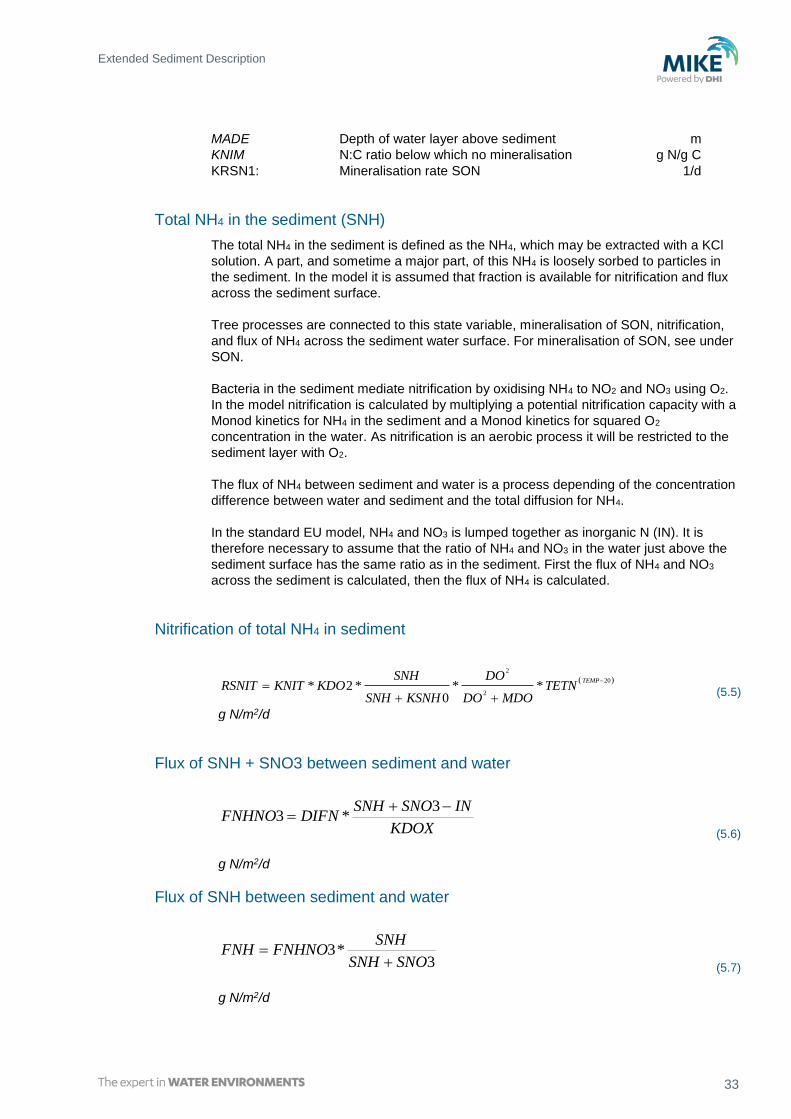
Extended Sediment Description
33
MADE Depth of water layer above sediment m
KNIM N:C ratio below which no mineralisation g N/g C
KRSN1: Mineralisation rate SON 1/d
Total NH4 in the sediment (SNH)
The total NH4 in the sediment is defined as the NH4, which may be extracted with a KCl
solution. A part, and sometime a major part, of this NH4 is loosely sorbed to particles in
the sediment. In the model it is assumed that fraction is available for nitrification and flux
across the sediment surface.
Tree processes are connected to this state variable, mineralisation of SON, nitrification,
and flux of NH4 across the sediment water surface. For mineralisation of SON, see under
SON.
Bacteria in the sediment mediate nitrification by oxidising NH4 to NO2 and NO3 using O2.
In the model nitrification is calculated by multiplying a potential nitrification capacity with a
Monod kinetics for NH4 in the sediment and a Monod kinetics for squared O2
concentration in the water. As nitrification is an aerobic process it will be restricted to the
sediment layer with O2.
The flux of NH4 between sediment and water is a process depending of the concentration
difference between water and sediment and the total diffusion for NH4.
In the standard EU model, NH4 and NO3 is lumped together as inorganic N (IN). It is
therefore necessary to assume that the ratio of NH4 and NO3 in the water just above the
sediment surface has the same ratio as in the sediment. First the flux of NH4 and NO3
across the sediment is calculated, then the flux of NH4 is calculated.
Nitrification of total NH4 in sediment
2
20
2* 2 * * *
0
TEMPSNH DORSNIT KNIT KDO TETN
SNH KSNH DO MDO
g N/m2/d
(5.5)
Flux of SNH + SNO3 between sediment and water
KDOX
INSNOSNHDIFNFNHNO
3*3
g N/m2/d
(5.6)
Flux of SNH between sediment and water
3*3
SNOSNH
SNHFNHNOFNH
g N/m2/d
(5.7)
DHI Eutrophication Model 1 – Including Sediment and Benthic Vegetation
34 MIKE ECO Lab Template - © DHI
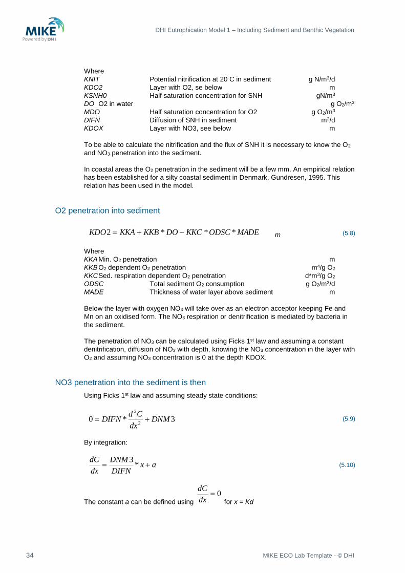
Where
KNIT Potential nitrification at 20 C in sediment g N/m3/d
KDO2 Layer with O2, se below m
KSNH0 Half saturation concentration for SNH gN/m3
DO O2 in water g O2/m3
MDO Half saturation concentration for O2 g O2/m3
DIFN Diffusion of SNH in sediment m2/d
KDOX Layer with NO3, see below m
To be able to calculate the nitrification and the flux of SNH it is necessary to know the O2
and NO3 penetration into the sediment.
In coastal areas the O2 penetration in the sediment will be a few mm. An empirical relation
has been established for a silty coastal sediment in Denmark, Gundresen, 1995. This
relation has been used in the model.
O2 penetration into sediment
MADEODSCKKCDOKKBKKAKDO ***2 m (5.8)
Where
KKA Min. O2 penetration m
KKB O2 dependent O2 penetration m4/g O2
KKC Sed. respiration dependent O2 penetration d*m3/g O2
ODSC Total sediment O2 consumption g O2/m3/d
MADE Thickness of water layer above sediment m
Below the layer with oxygen NO3 will take over as an electron acceptor keeping Fe and
Mn on an oxidised form. The NO3 respiration or denitrification is mediated by bacteria in
the sediment.
The penetration of NO3 can be calculated using Ficks 1st law and assuming a constant
denitrification, diffusion of NO3 with depth, knowing the NO3 concentration in the layer with
O2 and assuming NO3 concentration is 0 at the depth KDOX.
NO3 penetration into the sediment is then
Using Ficks 1st law and assuming steady state conditions:
3*02
2
DNMdx
CdDIFN
(5.9)
By integration:
axDIFN
DNM
dx
dC *
3 (5.10)
The constant a can be defined using
0dx
dC
for x = Kd

Extended Sediment Description
35
KdDIFN
DNMa *
3
(5.11)
By yet an integration, the concentration C can be found:
bxKdDIFN
DNMx
DIFN
DNMC **
3*
*2
3 2
(5.12)
The constant b can be defined using C = 0 for x = Kd.
2**2
3Kd
DIFN
DNMb
(5.13)
23
*2*3KDO
DNM
DIFNSNOKDOX
m
(5.14)
Where
DNM3. Denitrification g N/m3/d
DIFN Diffusion of NO3 in sediment m2/d
x Sediment depth, x=0 at KDO2 m
C Concentration of NO3 in sediment g NO3-N/m3
Kd Depth from KDO2 where NO3=0 m
NO3 in sediment (SNO3)
Three processes are determining the NO3 concentration in the sediment nitrification,
denitrification and flux of NO3 between sediment and water. The nitrification has been
described under SNH.
The flux of NO3 across the sediment surface is calculated in the same way as the flux of
NH4.
Flux of NO3 across sediment surface
FNHFNHNOFNO 33
g N/m2/d (5.15)
The denitrification (RDENIT) or flux of NO3 into the sediment is calculated using Ficks 1st
law.
Denitrification
dx
dCDIFNRDENIT *
for x = 0
(5.16)
For dx
dC
see under NO3 penetration into sediment

DHI Eutrophication Model 1 – Including Sediment and Benthic Vegetation
36 MIKE ECO Lab Template - © DHI
3**2 DNMDIFNRDENIT (5.17)
Where
20*3 TEMPTETNDEMAXDNM
g N/m2/d (5.18)
Immobilisation of N in sediment (SNIM)
Immobilisation of N may occur either as burial of slowly degradable organic N or as
denitrification of NO3. The processes have been described under SON and SNO3
respectively.
5.3 Phosphorus Processes
The below description of the phosphorus processes is made according to the state
variables in the P cycle.
Leachable organic P in sediment (SOP)
SOP is a pool of leachable organic P, which is able to be turned into PO4 by
mineralisation. Input to SOP occur through sedimentation of algae P and detritus P to the
sediment surface, a fraction of the settled organic P in mineralised on the sediment
surface represented by the flux FSPB. However a part of the settled P will be immobilised
in the sediment either as refractive organic P or as apatite P. In the model the
immobilisation is calculated as a fraction of RSOP which enters the pool of immobilised P,
SIMP. The remaining of the settled organic P enters SOP
Mineralisation of newly settled organic P
20**0 TEMPTRSPSEEPSEPPSEDPKRESPFSPB
g P/m3/d
(5.19)
Input of P to sediment pool of organic P
MADEFSPBSEEPSEDPSEPPRSOP *
g P/m2/d
(5.20)
Burial of organic P in sediment
KPIMRSOPRSPIM *
g P/m2/d (5.21)

Extended Sediment Description
37
Mineralisation of SOP in the sediment
20*1* TEMPTRSPKRSPSOPROPSIP g P/m2/d (5.22)
Where
KRESP0 Fraction mineralised at 20 C
SEPP Sedimentation of PP (plankton P), g P/m3/d
SEDP Sedimentation of DP (detritus P), g P/m3/d
SEEP Input to sediment of P in dead eelgrass, (option) g P/m3/d
TEMP Water temperature, C
MADE Dept of water layer above sediment m
KRSP1 Mineralisation rate SOP 1/d
PO4 in pore water (SIP) and PO4 adsorbed to Fe+++ (SPFE)
PO4 in pore water may either adsorbed to Fe+++ (SPFE) or exchanged with PO4 in the
water across the sediment surface. The equilibrium of PO4 adsorbed to Fe+++ is
described as a product between a P sorption capacity, which is depending of the amount
of F+++, and a Monod relation of SIP, Jacobsen, 1997 and 1998.
The adsorption or desorption of PO4 is then defined as the change in SPFE caused by a
change the concentration of SIP or a change in the amount of Fe+++, which is dependent
of the penetration depth of NO3. (KDOX).
Sorption and desorption of PO4 to Fe+++
6
1
*( * * * * *10
* )t
RFESIP KRAP
SIPKFE KFEPO VF DM
SIP KHFE
KDOX SPFE
g P/m2/d (5.23)
Flux of PO4 between sediment and water
KDOX
IPSIPKFIPFSIP
*
g P/m2/d
(5.24)
Where
DM Dry matter of sediment, specified by user g DM/g ww
VF Specific gravity, specified by user g ww/cm3
SPFEt-1 SPFE to time t-1 g P/m2

DHI Eutrophication Model 1 – Including Sediment and Benthic Vegetation
38 MIKE ECO Lab Template - © DHI
5.4 Differential Equations
The change in the state variable with time is calculated by adding all the processes
together in a differential equation set up for each state variable.
Below the differential equations are defined:
RSNIMRSONNHRSONdt
dSON
g N/m2/d
(5.25)
2**1 KDOVFDM
FNHRSNITRSONNH
dt
dSNH
g N/m3/d
(5.26)
KDSVFDM
FNORDENITRSNIT
dt
dSNO
**1
33
g N/m3/d
(5.27)
RDENITRSNIMdt
dSNIM
g N/m2/d
(5.28)
RSPIMROPSIPRSOPdt
dSOP
g P/m2/d
(5.29)
KDSVFDM
FSIPROPSIPRFESIP
dt
dSIP
**1
g P/m3/d
(5.30)
RFESIPdt
dSPFE
g P/m2/d
(5.31)
RSPIMdt
dSPIM
g P/m2/d
(5.32)
Where
DM Dry matter of sediment, specified by user g DM/g ww
VF Specific gravity, specified by user g ww/cm3
KDS Depth of active sediment layer, specified by user m
Extended Sediment Description
39
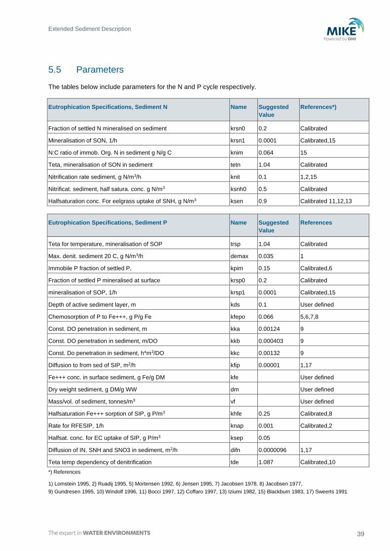
5.5 Parameters
The tables below include parameters for the N and P cycle respectively.
Eutrophication Specifications, Sediment N Name Suggested
Value
References*)
Fraction of settled N mineralised on sediment krsn0 0.2 Calibrated
Mineralisation of SON, 1/h krsn1 0.0001 Calibrated,15
N:C ratio of immob. Org. N in sediment g N/g C knim 0.064 15
Teta, mineralisation of SON in sediment tetn 1.04 Calibrated
Nitrification rate sediment, g N/m3/h knit 0.1 1,2,15
Nitrificat. sediment, half satura. conc. g N/m3 ksnh0 0.5 Calibrated
Halfsaturation conc. For eelgrass uptake of SNH, g N/m3 ksen 0.9 Calibrated 11,12,13
Eutrophication Specifications, Sediment P Name Suggested
Value
References
Teta for temperature, mineralisation of SOP trsp 1.04 Calibrated
Max. denit. sediment 20 C, g N/m3/h demax 0.035 1
Immobile P fraction of settled P, kpim 0.15 Calibrated,6
Fraction of settled P mineralised at surface krsp0 0.2 Calibrated
mineralisation of SOP, 1/h krsp1 0.0001 Calibrated,15
Depth of active sediment layer, m kds 0.1 User defined
Chemosorption of P to Fe+++, g P/g Fe kfepo 0.066 5,6,7,8
Const. DO penetration in sediment, m kka 0.00124 9
Const. DO penetration in sediment, m/DO kkb 0.000403 9
Const. Do penetration in sediment, h*m3/DO kkc 0.00132 9
Diffusion to from sed of SIP, m2/h kfip 0.00001 1,17
Fe+++ conc. in surface sediment, g Fe/g DM kfe User defined
Dry weight sediment, g DM/g WW dm User defined
Mass/vol. of sediment, tonnes/m3 vf User defined
Halfsaturation Fe+++ sorption of SIP, g P/m3 khfe 0.25 Calibrated,8
Rate for RFESIP, 1/h knap 0.001 Calibrated,2
Halfsat. conc. for EC uptake of SIP, g P/m3 ksep 0.05
Diffusion of IN, SNH and SNO3 in sediment, m2/h difn 0.0000096 1,17
Teta temp dependency of denitrification tde 1.087 Calibrated,10
*) References
1) Lomstein 1995, 2) Ruadij 1995, 5) Mortensen 1992, 6) Jensen 1995, 7) Jacobsen 1978, 8) Jacobsen 1977,
9) Gundresen 1995, 10) Windolf 1996, 11) Bocci 1997, 12) Coffaro 1997, 13) Iziumi 1982, 15) Blackburn 1983, 17) Sweerts 1991

DHI Eutrophication Model 1 – Including Sediment and Benthic Vegetation
40 MIKE ECO Lab Template - © DHI

Future Developments
41
6 Future Developments
Future versions of MIKE 21/3 EU will provide the possibility of including modules for
filtrators (mussels etc.), feed-back from sediment spills. Also a flexible ecosystem
description that can be defined and edited by the user will be developed.

DHI Eutrophication Model 1 – Including Sediment and Benthic Vegetation
42 MIKE ECO Lab Template - © DHI

Solution Technique
43
7 Solution Technique
The solution of the set of ordinary coupled differential equations is found using an
integration routine in an integrated two-step procedure with the AD module.
The results give a resolution in space and time depending on the details of the chosen
grid and the time step used.

DHI Eutrophication Model 1 – Including Sediment and Benthic Vegetation
44 MIKE ECO Lab Template - © DHI

Data Requirements
45
8 Data Requirements
• Basic Model Parameters
- Model grid size and extent
- Time step and length of simulation
- Type of output required and its frequency
• Bathymetry and Hydrodynamic Input
• Combined Advection-Dispersion Model
- Dispersion coefficients
• Initial Conditions
- Concentration of parameters
• Boundary Conditions
- Concentration of parameters
• Pollution Sources
- Discharge magnitudes and concentration of parameters
• Process Rates
- Size of coefficients governing the process rates. Some of these coefficients can
be determined by calibration. Others will be based on literature values or found
from actual measurements and laboratory tests.

DHI Eutrophication Model 1 – Including Sediment and Benthic Vegetation
46 MIKE ECO Lab Template - © DHI

List of References
47
9 List of References
/1/ Bach, H.K., D. Orhon, O.K. Jensen & I.S. Hansen. Environmental Model studies
for the Istanbul Master Plan. Part II: Water Quality and Eutrophication.
Wat.Sci.Tech. Vol. 32, No. 2, pp 149-158, 1995.
/2/ Bach, H., A. Malmgren-Hansen and J. Birklund. Modelling of Eutrophication
Effects on Coastal Ecosystems with Eelgrass as the Dominating Macrophyte.
Presented at the Int. Conf. on Marine Coastal Eutrophication, Bologna, 21-23
March 1990.
/3/ Baker, E.T. and J.W. Lavelle. The Effect of Particle Size on the Light Attenuation
Coefficient of Natural Suspensions. J. of Geophysical Reas. Vol. 89, No. C5, pp
8197-8203, Sept. 1984.
/4/ Blackburn T.H., Henriksen K. Nitogen cycling in different types of sediments
from Danish Waters Limnol. Oceanogr. 28(3), pp. 477-493.
/5/ Bocci M., Coffaro G., Bendoricchio G. Modelling biomass and nutrient dynamics
in eelgrass (Zostera marina): applications to Lagoon of Venice (Italy) and
Øresund (Denmark) Ecol. Model. 102, pp 67-80, 1997.
/6/ Canale, R.P. and Martin T. Aues. Ecological Studies and Mathematical
Modelling of Cladophora in Lake Huron: 5. Model Development and Calibration.
J. Great Lakes Res. 8(1), pp 112-125, 1982.
/7/ Coffaro G., Bocci M. 1997. Resources competition between Ulva rigida and
Zostera marina: a quantitative approach applied to the Lagoon of Venice. Ecol.
Model. 102 PP 81-95, 1997
/8/ Dahl-Madsen, K.I. Mathematical Modelling of Eutrophied Coastal Areas. Prog.
Wat. Tech., Vol. 10, Nos. 5/6, pp 217-235, 1978.
/9/ Droop, M.R. Some thoughts on nutrient limitation in algae. J. Phycol. 9: 264-
272, 1973.
/10/ Droop, M.R. The nutrient status of algal cells in batch cultures. J. Mar. Biol. Ass.
U.K. 55: 541-555, 1975.
/11/ Goldman, Joel C. Outdoor Algal Mass Cultures- II Photosynthetic Yield
Limitations. Water Research, Vol. 13, pp 119-136, 1979.
/12/ Gordon, D.M., P.B. Birch and A.J. McComb. The effect of light, temperature,
and salinity on photosynthetic rates of an estuarine Cladophora. Bot. Mar. 23:
749-755, 1980.
/13/ Gundresen K.J., Glud R.N., Jørgensen B.B. Havbundens Iltomsætning.
Havforskning fra Miljøstyrelsen, nr. 57. 1995
/14/ Hobson, L.A. Effects of interaction of irradiance, daylength, and temperature on
division rates of three species of marine unicellular algae J. Fish. Res. Bd.
Canada 31: 391-395, 1974.
/15/ Horwood, J.W. A model of primary and secondary production. ICES C.M.
1974/L 19:1-10, 1974.

DHI Eutrophication Model 1 – Including Sediment and Benthic Vegetation
48 MIKE ECO Lab Template - © DHI
/16/ Ichimura, S. Environmental gradient and its relation to primary productivity in
Tokyo Bay. Records Oceanogr. Works (Japan) 9: 115-128, 1967.
/17/ Iziumi H., Hattori A. Growth and organic production of eelgrass (Zostera marina)
in temperate waters of the pacific coast of Japan. III The kinetics of nitrogen
uptake. Aquat. Bot. 12, pp. 245-256, 1982.
/18/ Jacobsen O.S. Sorption, adsorption and chemosorption of phosphate by Danish
lake sediments Vatten nr. 4, PP 230-241, 1978
/19/ Jacobsen O.S. Sorption of phosphate by Danish Lake Sediments Vatten nr. 3,
PP 290-298, 1977.
/20/ Jassby, A.D. and C.R. Goldman. Loss rates from a lake phytoplankton
community. Limnol. Oceanogr. 21: 540-547, 1974.
/21/ Jensen H.S., Mortensen P.B., Andersen F.Ø, Rasmussen E.K., A. Jensen,
1995. Phosphorus cycling in cosatal marine sediment. Limnol. Oceanogr. 40(5),
PP 908-917.1995.
/22/ Lancelot, C. and V. Rousseau. ICES intercalibration exercise on the 14C
method for estimating phytoplankton primary production. Phase 2: experiments
conducted on board of RV DANA. Preliminary report, 35 pp, 1987.
/23/ Lancelot, C, G. Billen, A. Sourina, T. Weisse, F. Colijn, M.J.W. Veldhuis, A.
Davies and P. Wassman. Phaeocystis blooms and nutrient enrichment in the
continental coastal zones of the North Sea. Ambio 16: 38-46, 1987.
/24/ Lomstein, Bente et al. Omsætning af organisk kvælstof i marine sedimenter.
Havforskning fra Miljøstyrelsen nr. 58. 1995
/25/ Mommaerts, J.P. Systeembenadering van en gesloten mariene milieu, met de
nadruk op de rol van het fytoplankton. Doctoral thesis. Vrije Universiteit Brussel:
1-335, 1978.
/26/ Mortensen P.B., Jensen H.S., Rasmussen E.K., Østergaard Andersen P.
Fosforomsætning i sedimentet i Århus Bugt. Havforskning fra Miljøstyrelsen, nr.
17. 1992.
/27/ Nyholm, Niels. A Mathematical Model for the Growth of Phytoplankton.
Presented at the Int. Symp. on Experimental Use of Algal Cultures in Limnology,
Sandefjord, Norway, Oct. 26-28 1976.
/28/ Nyholm, N. Kinetics of phosphate-limited algal growth. Biotechn. Bioengineering
19: 467-492, 1977.
/29/ Nyholm, Niels. A Simulation Model for Phytoplankton Growth Cycling in
Eutrophic Shallow Lakes. Ecological Modelling, Vol. 4, pp 279-310, 1978.
/30/ Nyholm, Niels. The Use of Management Models for Lakes at the Water Quality
Institute, Denmark. State-of-the-art in Ecological Modelling, Vol. 7, pp 561-577,
1979.
/31/ Press, W.H., B.P. Flannery, S.A. Teukolsky and W.T. Vetterling. Numerical
Recipes. Cambridge University Press (1986). Press.
List of References
49
/32/ Ruadij P., W.Van Raaphorst, 1995 Benthic nutrient regeneration in the ERSEM
ecosystem model of the North SeaNetherlands Journal of Sea Research, 33
(3/4) PP 453-483, 1995
/33/ Scavia, Donald. Examination of Phosphorus Cycling and Control of
Phytoplankton Dynamics in Lake Ontario with an Ecological Model. J. Fish. Res.
Board Can., Vol. 36, pp 1336-1346, 1979.
/34/ Schnorr, J.L. and D.M. Di Toro. Differential Phytoplankton Sinking- and Growth
Rates: an Eigenvalue Analysis. Ecological Modelling, Vol. 9, pp 233-245, 1979.
/35/ Smayda, T.J. The suspension and sinking of phytoplankton in the sea.
Oceanogr. Mar. Biol. Ann. Rev. 8: 357-414, 1970.
/36/ Steele, J.H. The role of predation in ecosystem models. Marin. Biol. 35: 9-11,
1976.
/37/ Steemann Nielsen, E. and E.G. Jørgensen. The adaptation of plankton algae.
III. With special consideration of the importance in nature. Physiol. Plant. 21:
647-654, 1968.
/38/ Swartzman, Gordon L., and Richard Bentley. A Review and Comparison of
Plankton Simulation Models. ISEM Journal 1, Nos. 1-2, pp 30-81, 1979.
/39/ Sweerts et all. Similarity of whole-sediment molecular diffusion coefficients in
fresh water sediments of low and high porosity. Limnol. Oceanogr. 36 (2), pp.
336-341, 1991.
/40/ Tett, P., A. Edwards and K. Jones. A model for the growth of shelf-sea
phytoplankton in summer. Estuar. Coast. Shelf Sci. 23: 641-672, 1986.
/41/ Valiela, I.Marine ecological processes. ISBN 3-540-90929-X, Springer-Verlag,
New York, 1984.
/42/ Wetzel, R.L., R.F. van Tine and P.A. Penhale. Light and Submerged
Macrophyte Communities in Chesapeake Bay: A Scientific Summary. Report of
the Chesapeak Bay Programme, Virginia Institute of Marine Science, 1981.
/43/ Sundby Bjørn, Gobeil C., Silverberg N. The Phosphorus cycle in coastal marine
sediments.Limnol. Oceanogr. 37 (6), pp. 1129-1145. 1992.
/44/ Williams, P.J. LEB. Aspects of dissolved organic material in sea water. In: J.P.
Riley & G. Skirrow. Chemical Oceanography. Academic Press, New York: 301-
363, 1975.
/45/ Windolf J, Jeppesen E., Jensen J.P. Kristensen P.1996. Modelling of seasonal
variation in nitrogen retention and in-lake concentration: A four-year mass
balance study in 16 shallow Danish Lakes. Biogeochemistery 33, PP 25-
44.1996

DHI Eutrophication Model 1 – Including Sediment and Benthic Vegetation
50 MIKE ECO Lab Template - © DHI