DG-FEM for Time-Dependent Problems Lecture 1: The Basics

DG-FEM for Time-Dependent ProblemsLecture 1: The Basics

Jan S. Hesthaven

[email protected]

www.cfm.brown.edu/people/jansh/

Division of Applied Mathematics

Brown University, Box F

Providence, RI 02912, USA

Ecole de Ondes, INRIA 2006 – p.1

Let Me Start by Saying Thank you!

To the organizersGary CohenPatrick Joly

To the people payingINRIA, CEA, EDFNSF, DARPA, Sloan Foundation

To collaboratorsTim WarburtonLucas Wilcox, Gustaav Jacobs, David Gottlieb. . . and many others !

. . . and to you all for coming !


Focus of My Lectures

Time-depedent wave equations

Mostly linear problems but also some nonlinear problems

We shall discuss mainly DG-FEM but also some generalissues of finite volume methods for conservation laws

I shall strive to blend theory and applications with proofsbeing sketchy at best

Caution with the notes

. . . and the codes


The Grand Picture

Lecture 1: The Basics

The why’s, how’s, and what’s

Lecture 2: Insight through theory and some practicalities

A deeper look behind the scenes and some basicimplementation details

Lecture 3: Extensions to 2D/3D

Extending it all to 2D/3D, Maxwell’s equations andsome problems

Lecture 4: Problems with variable coefficients andnonlinear terms

What happens – and how do we control it ?


Overview of Lecture 1

Why do we need something else ?Pros’ and Con’s of existing methodsWishlistWhy is high-order important ?

The first schemeCentral elementsRole of numerical flux’Experimental’ evidence

GeneralizationsSystems and multiple dimensionsFluxes for linear systems


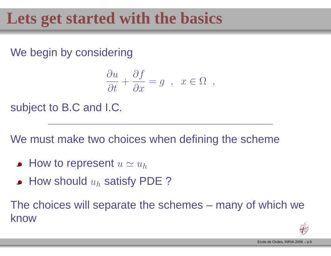
Lets get started with the basics

We begin by considering

∂u

∂t+∂f

∂x= g , x ∈ Ω ,

subject to B.C and I.C.

We must make two choices when defining the scheme

How to represent u ≃ uh

How should uh satisfy PDE ?

The choices will separate the schemes – many of which weknow


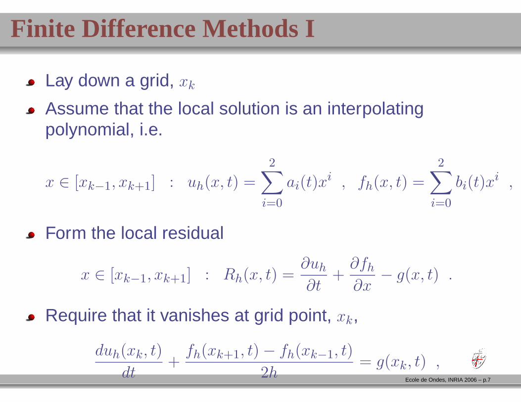
Finite Difference Methods I

Lay down a grid, xk

Assume that the local solution is an interpolatingpolynomial, i.e.

x ∈ [xk−1, xk+1] : uh(x, t) =2∑

i=0

ai(t)xi , fh(x, t) =

2∑

i=0

bi(t)xi ,

Form the local residual

x ∈ [xk−1, xk+1] : Rh(x, t) =∂uh

∂t+∂fh

∂x− g(x, t) .

Require that it vanishes at grid point, xk,

duh(xk, t)

dt+fh(xk+1, t) − fh(xk−1, t)

2h= g(xk, t) ,


Finite Difference Methods II

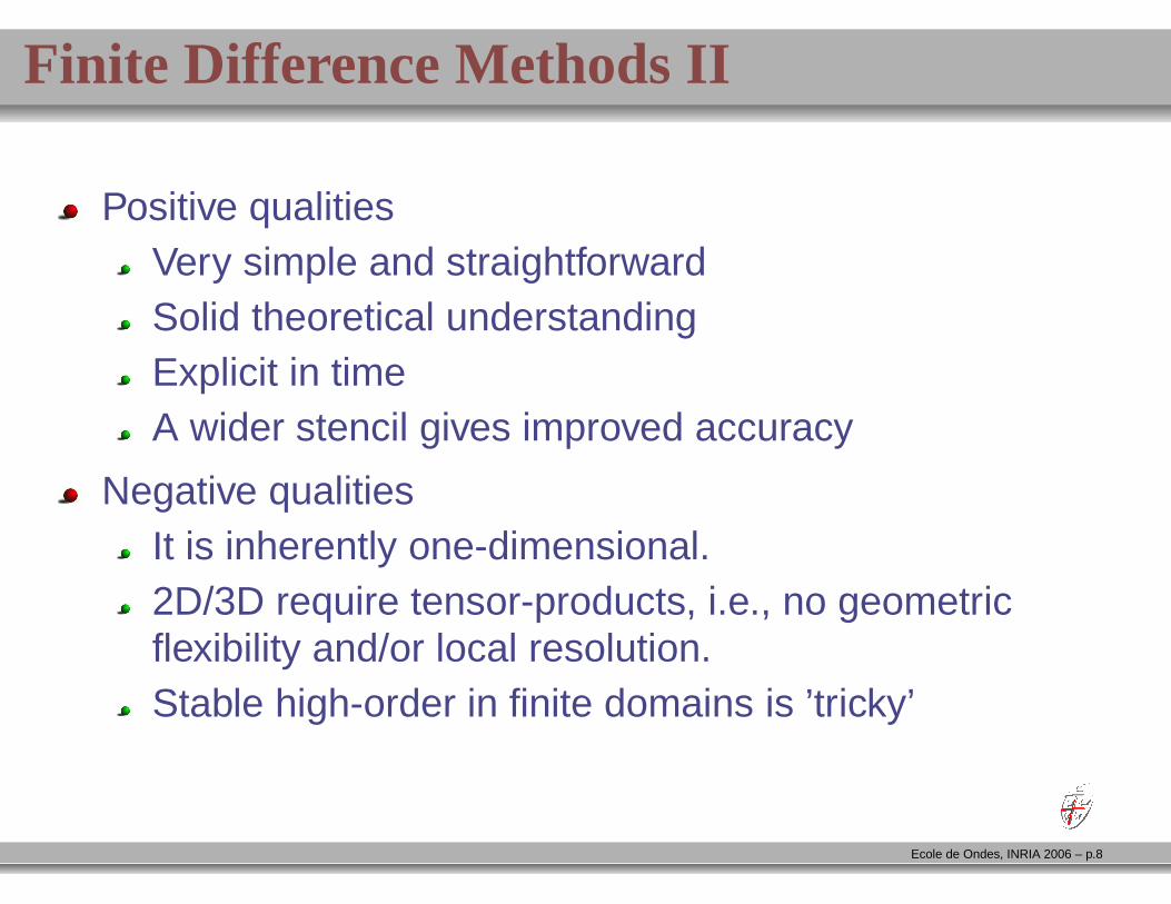
Positive qualitiesVery simple and straightforwardSolid theoretical understandingExplicit in timeA wider stencil gives improved accuracy

Negative qualitiesIt is inherently one-dimensional.2D/3D require tensor-products, i.e., no geometricflexibility and/or local resolution.Stable high-order in finite domains is ’tricky’


Observations

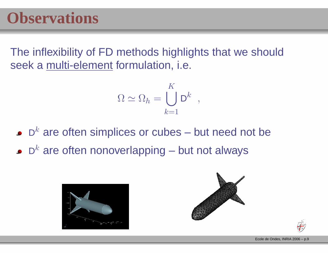
The inflexibility of FD methods highlights that we shouldseek a multi-element formulation, i.e.

Ω ≃ Ωh =K⋃

k=1

Dk ,

Dk are often simplices or cubes – but need not be

Dk are often nonoverlapping – but not always


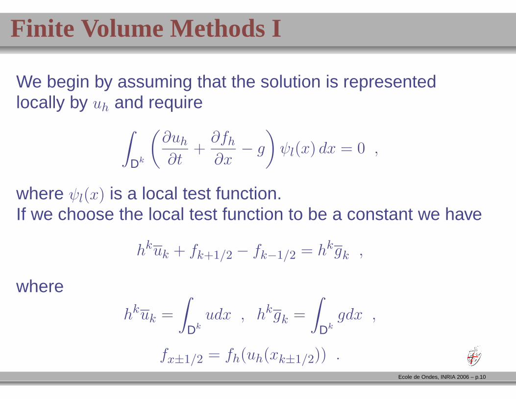
Finite Volume Methods I

We begin by assuming that the solution is representedlocally by uh and require

∫

Dk

(

∂uh

∂t+∂fh

∂x− g

)

ψl(x) dx = 0 ,

where ψl(x) is a local test function.If we choose the local test function to be a constant we have

hkuk + fk+1/2 − fk−1/2 = hkgk ,

where

hkuk =

∫

Dk

udx , hkgk =

∫

Dk

gdx ,

fx±1/2 = fh(uh(xk±1/2)) .


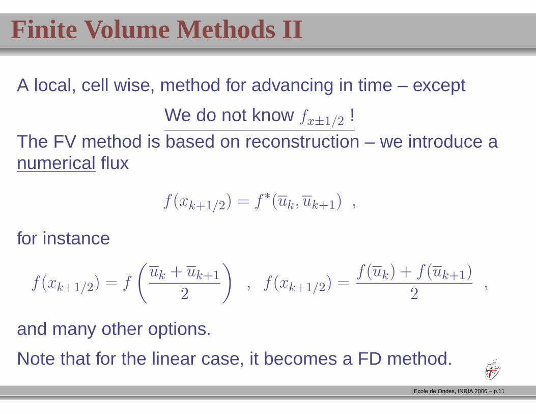
Finite Volume Methods II

A local, cell wise, method for advancing in time – except

We do not know fx±1/2 !

The FV method is based on reconstruction – we introduce anumerical flux

f(xk+1/2) = f∗(uk, uk+1) ,

for instance

f(xk+1/2) = f

(

uk + uk+1

2

)

, f(xk+1/2) =f(uk) + f(uk+1)

2,

and many other options.

Note that for the linear case, it becomes a FD method.


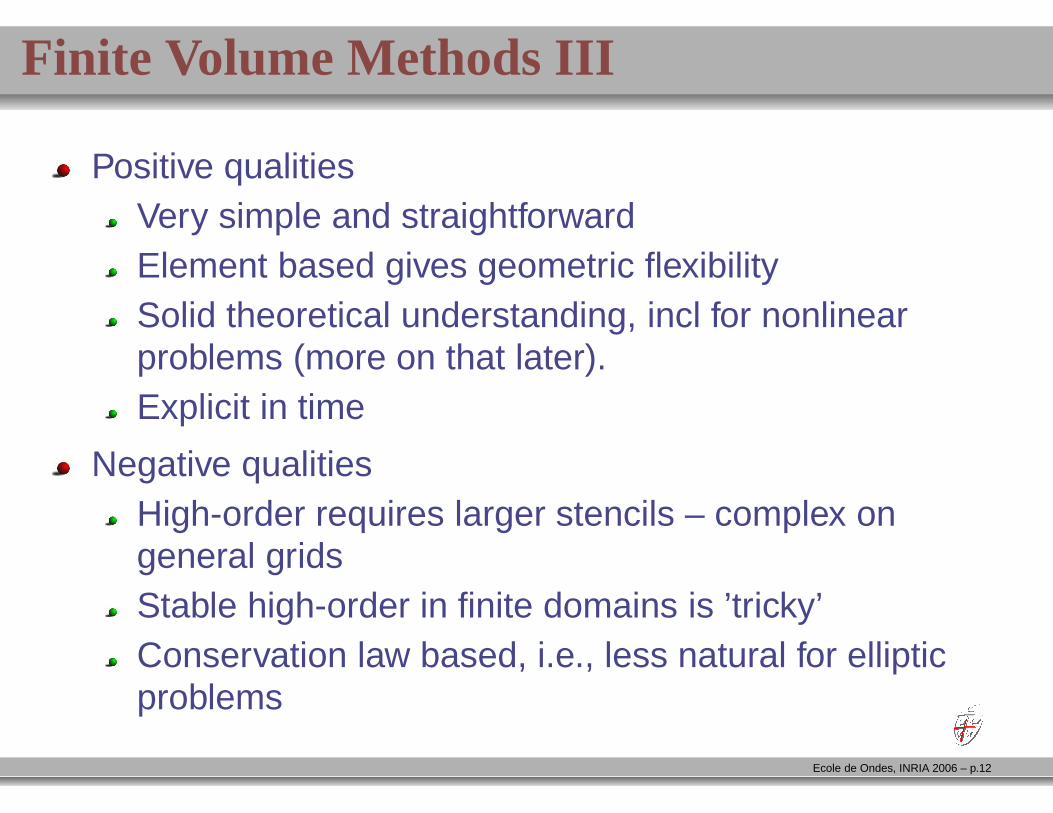
Finite Volume Methods III

Positive qualitiesVery simple and straightforwardElement based gives geometric flexibilitySolid theoretical understanding, incl for nonlinearproblems (more on that later).Explicit in time

Negative qualitiesHigh-order requires larger stencils – complex ongeneral gridsStable high-order in finite domains is ’tricky’Conservation law based, i.e., less natural for ellipticproblems


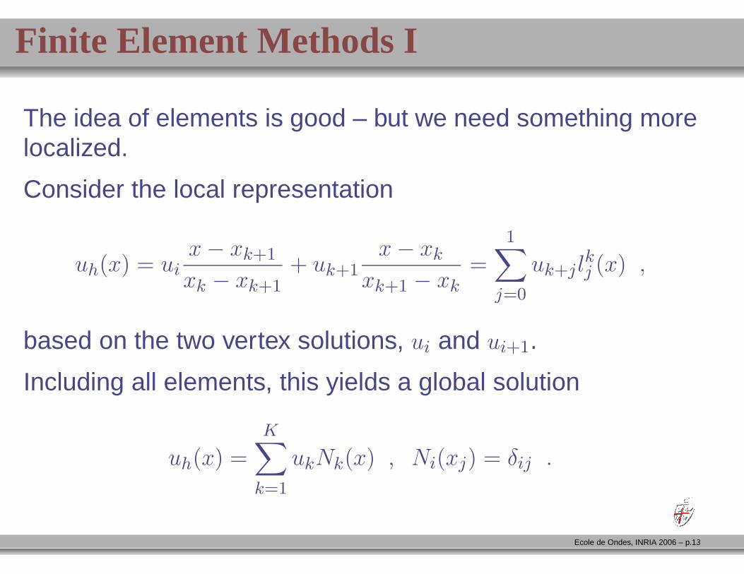
Finite Element Methods I

The idea of elements is good – but we need something morelocalized.

Consider the local representation

uh(x) = uix− xk+1

xk − xk+1+ uk+1

x− xk

xk+1 − xk=

1∑

j=0

uk+jlkj (x) ,

based on the two vertex solutions, ui and ui+1.

Including all elements, this yields a global solution

uh(x) =K∑

k=1

ukNk(x) , Ni(xj) = δij .


Finite Element Methods II

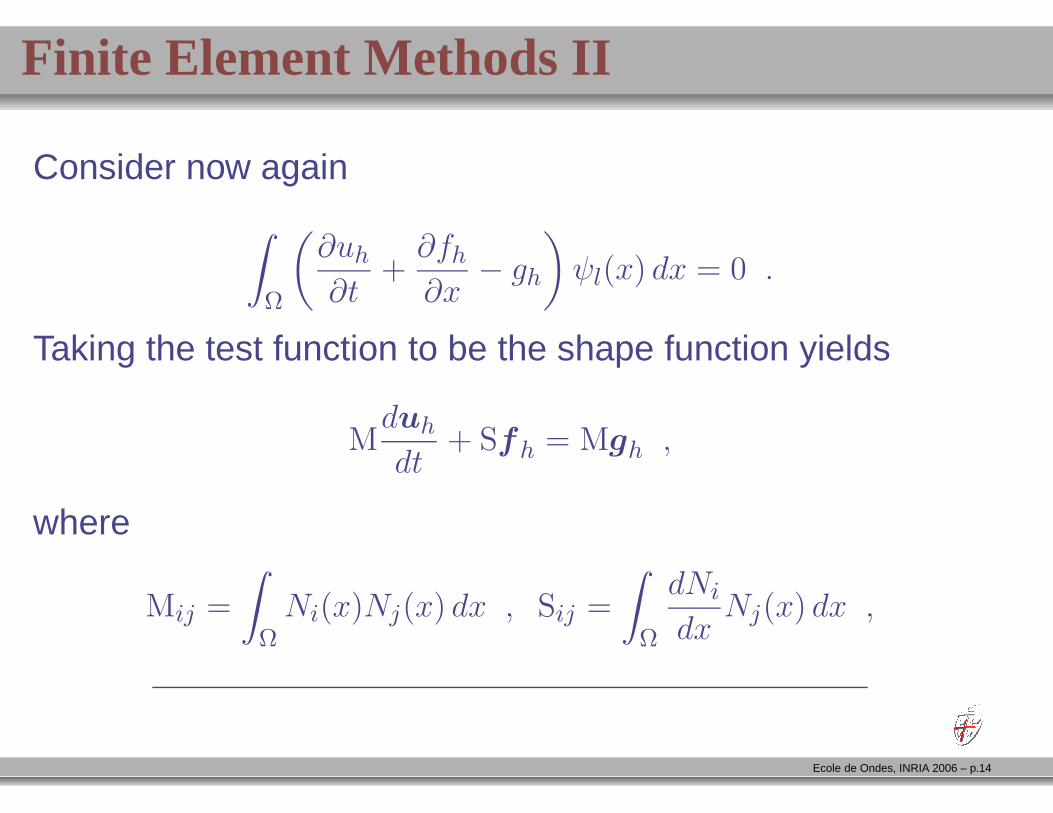
Consider now again

∫

Ω

(

∂uh

∂t+∂fh

∂x− gh

)

ψl(x) dx = 0 .

Taking the test function to be the shape function yields

Mduh

dt+ Sfh = Mgh ,

where

Mij =

∫

ΩNi(x)Nj(x) dx , Sij =

∫

Ω

dNi

dxNj(x) dx ,


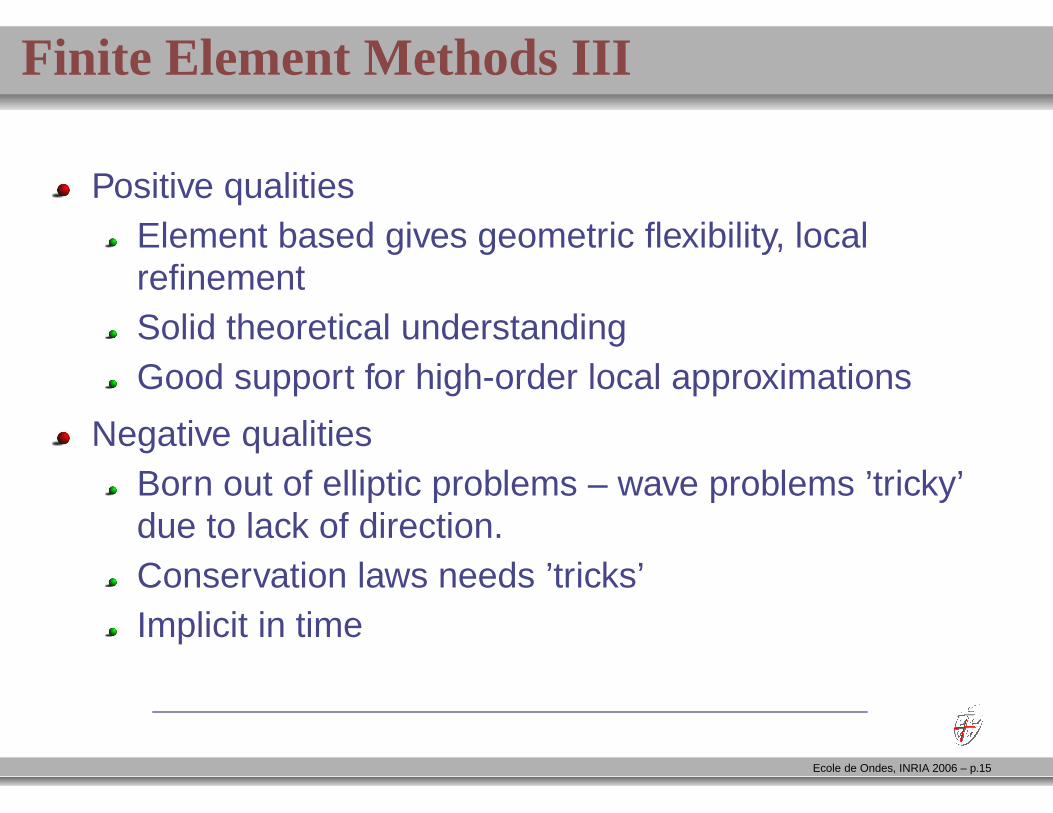
Finite Element Methods III

Positive qualitiesElement based gives geometric flexibility, localrefinementSolid theoretical understandingGood support for high-order local approximations

Negative qualitiesBorn out of elliptic problems – wave problems ’tricky’due to lack of direction.Conservation laws needs ’tricks’Implicit in time


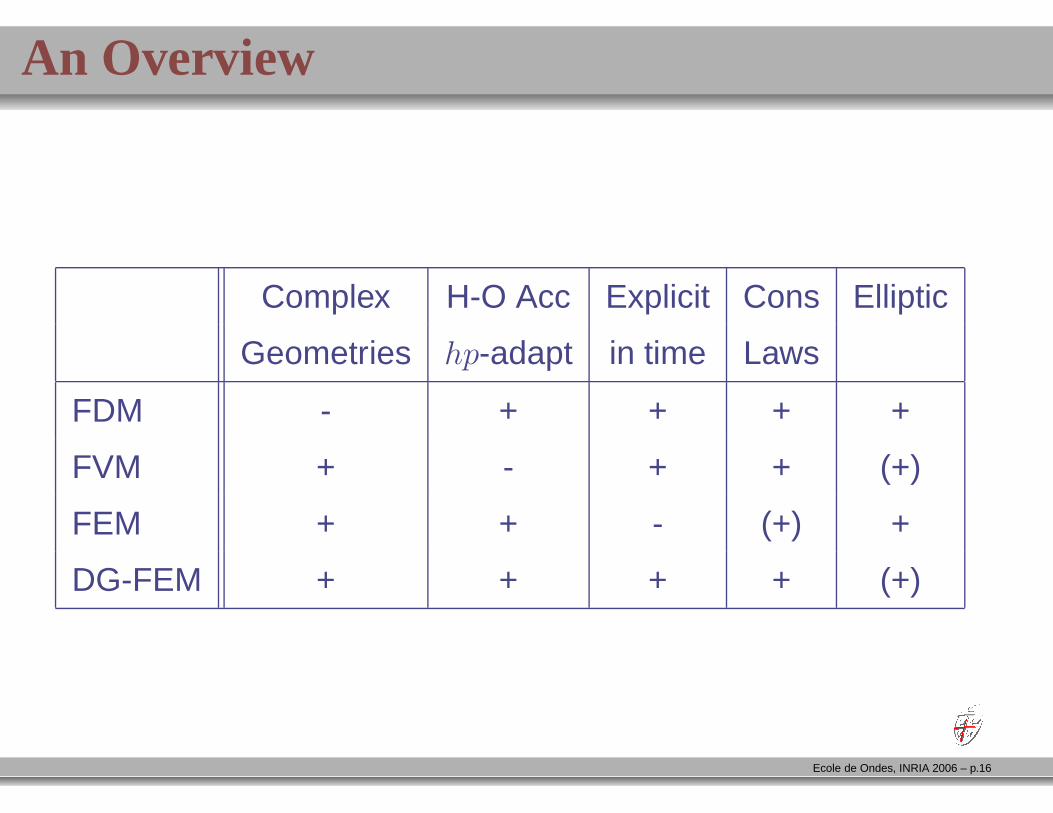
An Overview

Complex H-O Acc Explicit Cons Elliptic

Geometries hp-adapt in time Laws

FDM - + + + +

FVM + - + + (+)

FEM + + - (+) +

DG-FEM + + + + (+)


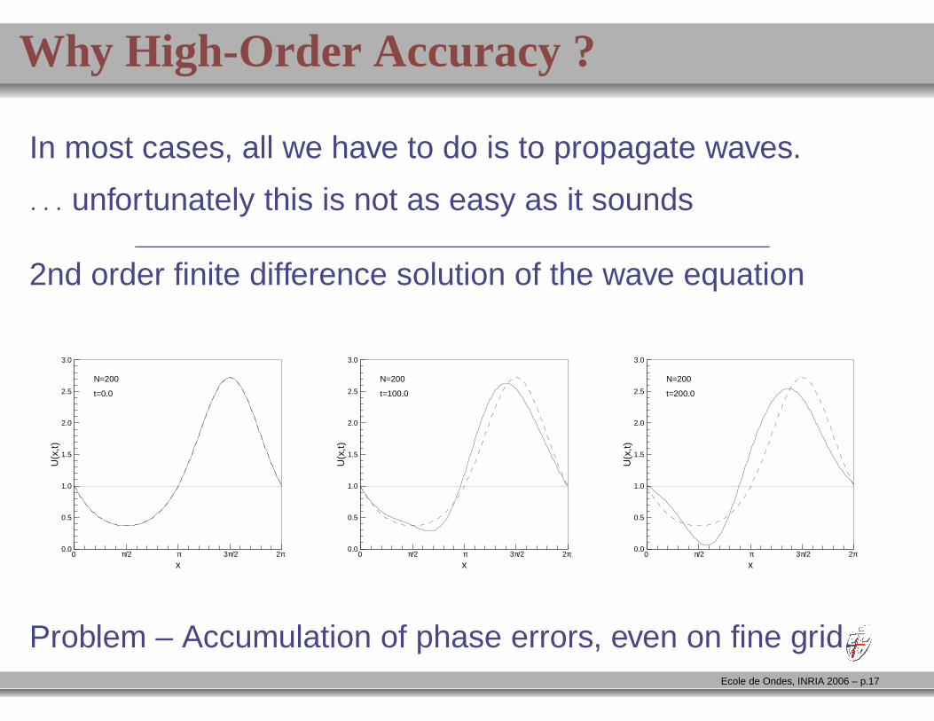
Why High-Order Accuracy ?

In most cases, all we have to do is to propagate waves.

. . . unfortunately this is not as easy as it sounds

2nd order finite difference solution of the wave equation

x

0.0

0.5

1.0

1.5

2.0

2.5

3.0

U(x

,t)

0 π/2 π 3π/2 2π

N=200

t=0.0

x

0.0

0.5

1.0

1.5

2.0

2.5

3.0

U(x

,t)

0 π/2 π 3π/2 2π

N=200

t=100.0

x

0.0

0.5

1.0

1.5

2.0

2.5

3.0

U(x

,t)

0 π/2 π 3π/2 2π

N=200

t=200.0

Problem – Accumulation of phase errors, even on fine grid.Ecole de Ondes, INRIA 2006 – p.17

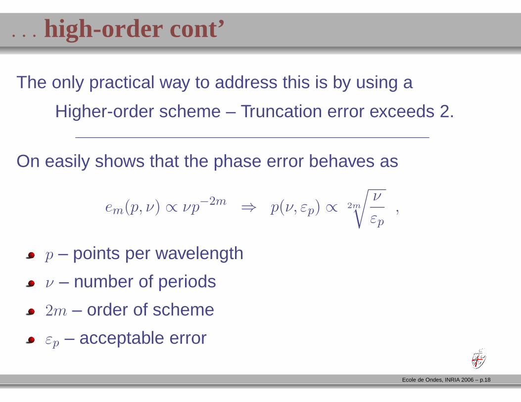
. . . high-order cont’

The only practical way to address this is by using a

Higher-order scheme – Truncation error exceeds 2.

On easily shows that the phase error behaves as

em(p, ν) ∝ νp−2m ⇒ p(ν, εp) ∝ 2m

√

ν

εp,

p – points per wavelength

ν – number of periods

2m – order of scheme

εp – acceptable error


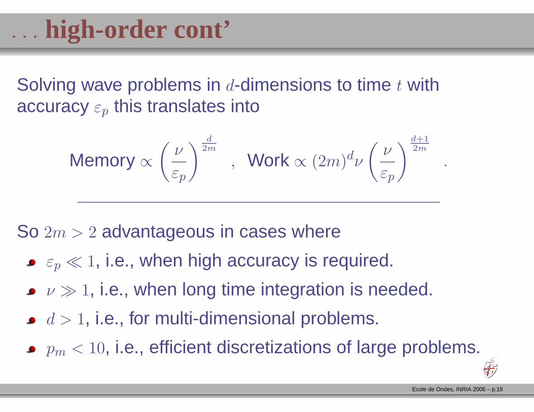
. . . high-order cont’

Solving wave problems in d-dimensions to time t withaccuracy εp this translates into

Memory ∝

(

ν

εp

)d

2m

, Work ∝ (2m)dν

(

ν

εp

)d+1

2m

.

So 2m > 2 advantageous in cases where

εp ≪ 1, i.e., when high accuracy is required.

ν ≫ 1, i.e., when long time integration is needed.

d > 1, i.e., for multi-dimensional problems.

pm < 10, i.e., efficient discretizations of large problems.


A Wishlist for a ’New’ Scheme

Support for high-order/non-uniform grids

Geometric flexibility

Suitable for both conservation laws and ’global’ problems

Explicit in time

Strong analysis basis

. . . and if we are greedy

Robustness to variations in equations

High computational efficiency


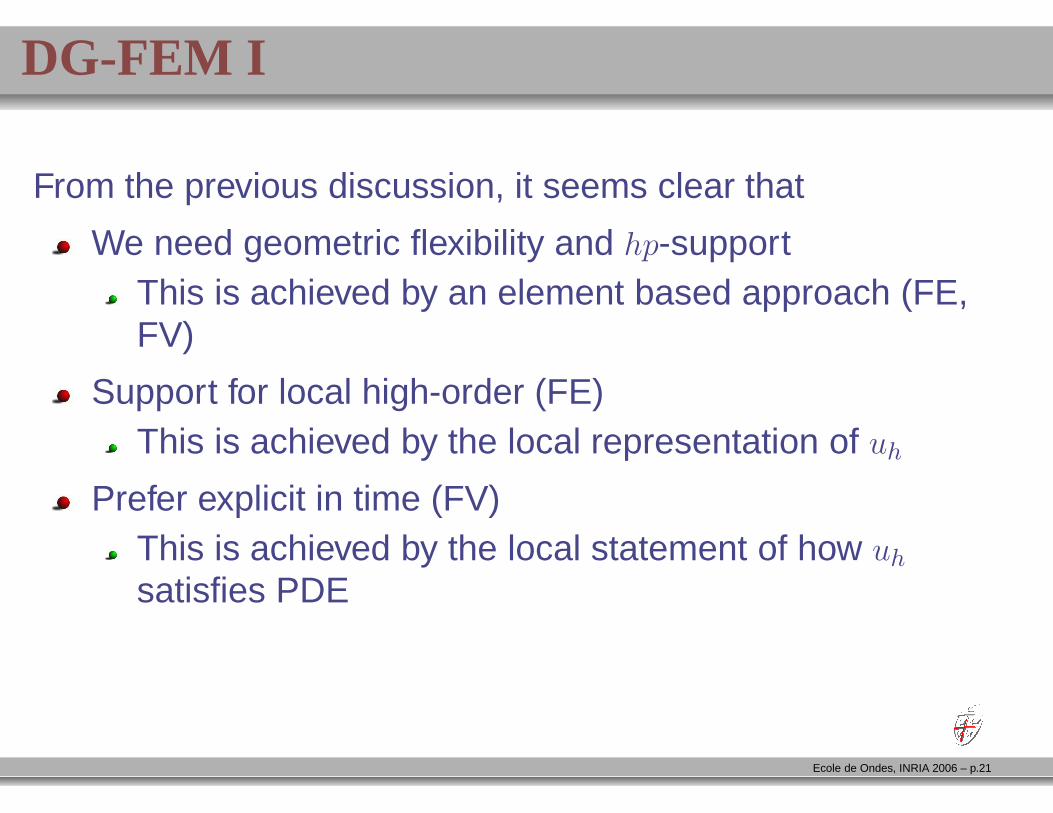
DG-FEM I

From the previous discussion, it seems clear that

We need geometric flexibility and hp-supportThis is achieved by an element based approach (FE,FV)

Support for local high-order (FE)This is achieved by the local representation of uh

Prefer explicit in time (FV)This is achieved by the local statement of how uh

satisfies PDE


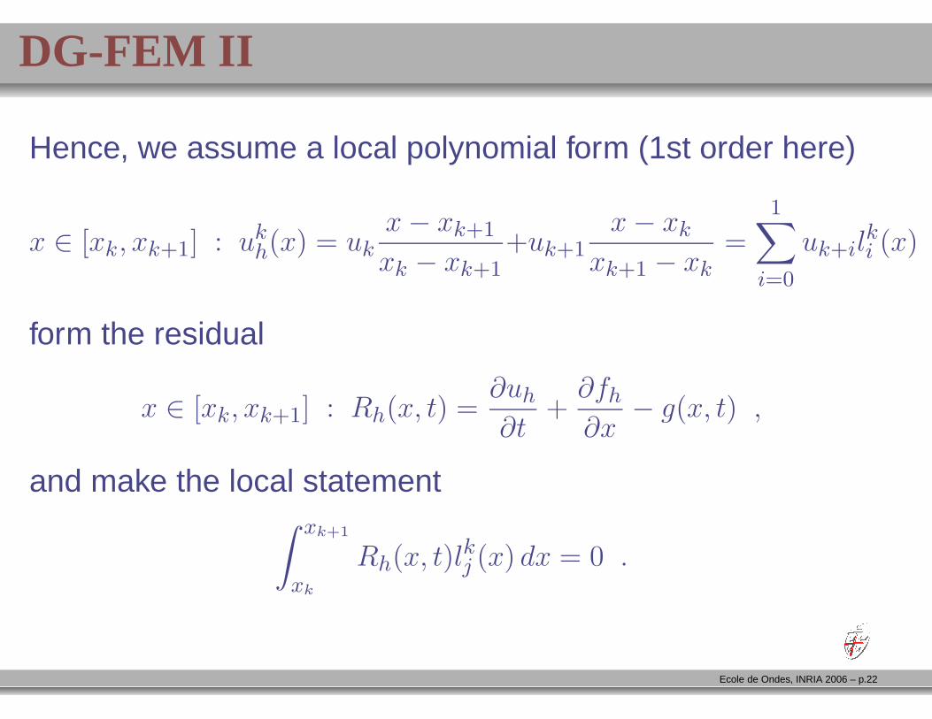
DG-FEM II

Hence, we assume a local polynomial form (1st order here)

x ∈ [xk, xk+1] : ukh(x) = uk

x− xk+1

xk − xk+1+uk+1

x− xk

xk+1 − xk=

1∑

i=0

uk+ilki (x)

form the residual

x ∈ [xk, xk+1] : Rh(x, t) =∂uh

∂t+∂fh

∂x− g(x, t) ,

and make the local statement∫ xk+1

xk

Rh(x, t)lkj (x) dx = 0 .


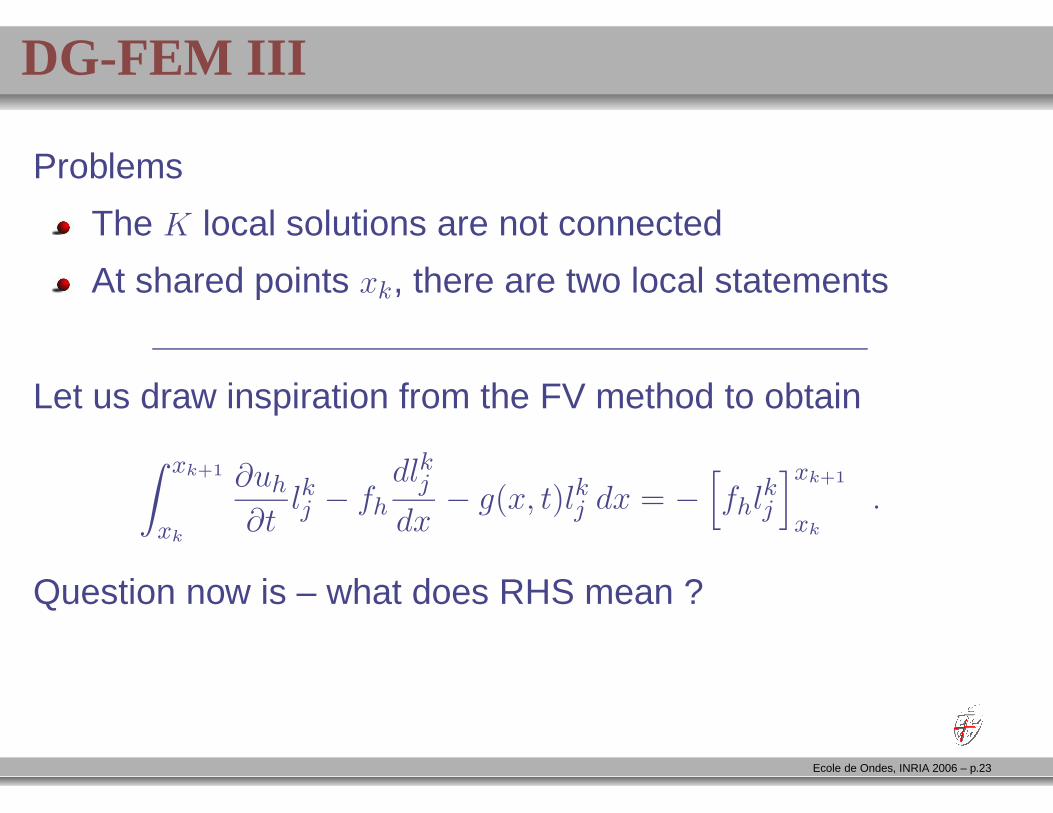
DG-FEM III

Problems

The K local solutions are not connected

At shared points xk, there are two local statements

Let us draw inspiration from the FV method to obtain

∫ xk+1

xk

∂uh

∂tlkj − fh

dlkj

dx− g(x, t)lkj dx = −

[

fhlkj

]xk+1

xk

.

Question now is – what does RHS mean ?


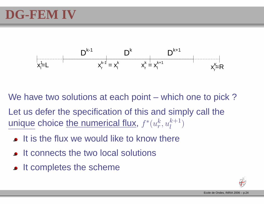
DG-FEM IV

Dk Dk+1Dk-1

x1l=L xK

r=Rxrk-1 = xl

k xrk = xl

k+1

We have two solutions at each point – which one to pick ?

Let us defer the specification of this and simply call theunique choice the numerical flux, f∗(uk

r , uk+1l )

It is the flux we would like to know there

It connects the two local solutions

It completes the scheme


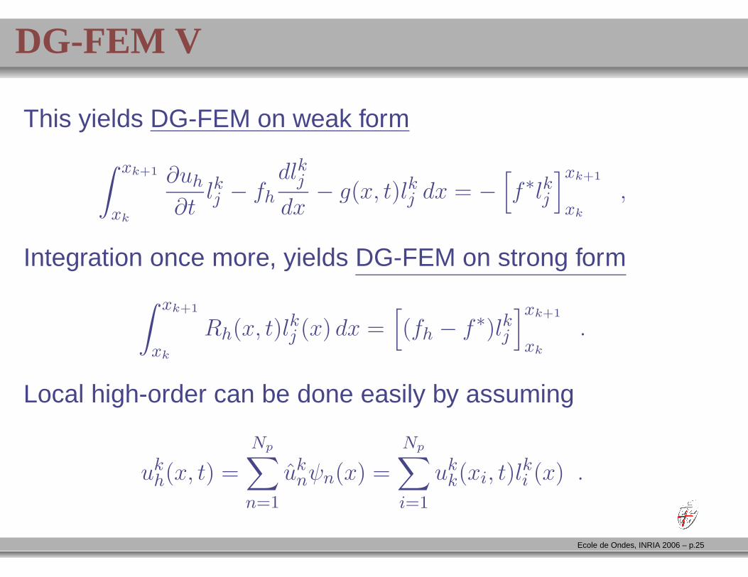
DG-FEM V

This yields DG-FEM on weak form

∫ xk+1

xk

∂uh

∂tlkj − fh

dlkj

dx− g(x, t)lkj dx = −

[

f∗lkj

]xk+1

xk

,

Integration once more, yields DG-FEM on strong form

∫ xk+1

xk

Rh(x, t)lkj (x) dx =[

(fh − f∗)lkj

]xk+1

xk

.

Local high-order can be done easily by assuming

ukh(x, t) =

Np∑

n=1

uknψn(x) =

Np∑

i=1

ukk(xi, t)l

ki (x) .


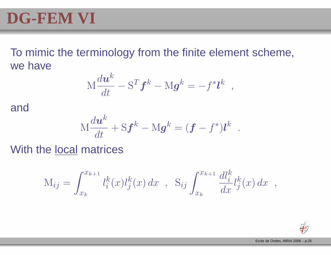
DG-FEM VI

To mimic the terminology from the finite element scheme,we have

Mduk

dt− STfk − Mgk = −f∗lk ,

and

Mduk

dt+ Sfk − Mgk = (f − f∗)lk .

With the local matrices

Mij =

∫ xk+1

xk

lki (x)lkj (x) dx , Sij

∫ xk+1

xk

dlkidxlkj (x) dx ,


DG-FEM VII

So we have a scheme which seems to catch the best of FEand FV

Element based to ensure geometric flexibility

Support for high-order by local basis

Local nature of scheme well suited for adaptivity

Explicit in time

Emerges from conservation laws, i.e., good for waves

Local in nature, i.e., high potential for parallel execution

This seems to violate the "no free lunch theorem" !

We pay with memory by dublicating surface modes


DG-FEM I – A Second View

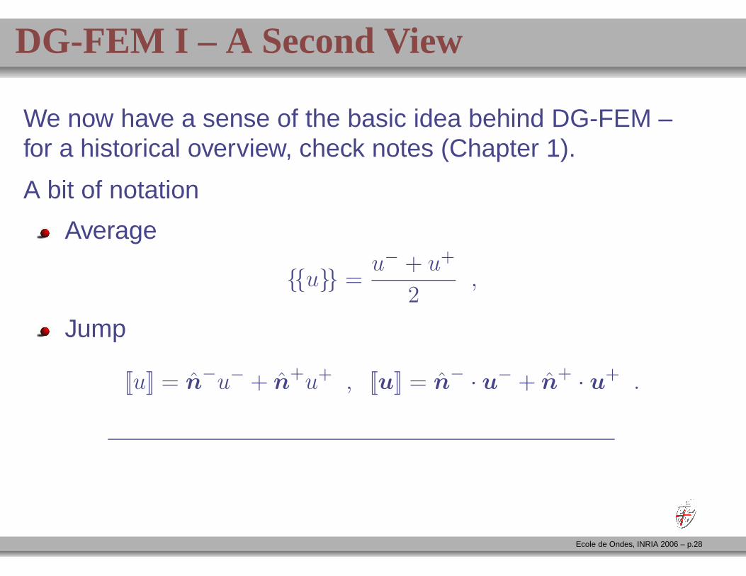
We now have a sense of the basic idea behind DG-FEM –for a historical overview, check notes (Chapter 1).

A bit of notation

Average

u =u− + u+

2,

Jump

[[u]] = n−u− + n+u+ , [[u]] = n− · u− + n+ · u+ .


DG-FEM II – A Second View

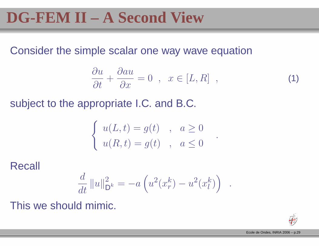
Consider the simple scalar one way wave equation

∂u

∂t+∂au

∂x= 0 , x ∈ [L,R] , (1)

subject to the appropriate I.C. and B.C.

u(L, t) = g(t) , a ≥ 0

u(R, t) = g(t) , a ≤ 0.

Recalld

dt‖u‖2

Dk = −a(

u2(xkr ) − u2(xk

l ))

.

This we should mimic.


DG-FEM III – A Second View

Dk Dk+1Dk-1

x1l=L xK

r=Rxrk-1 = xl

k xrk = xl

k+1

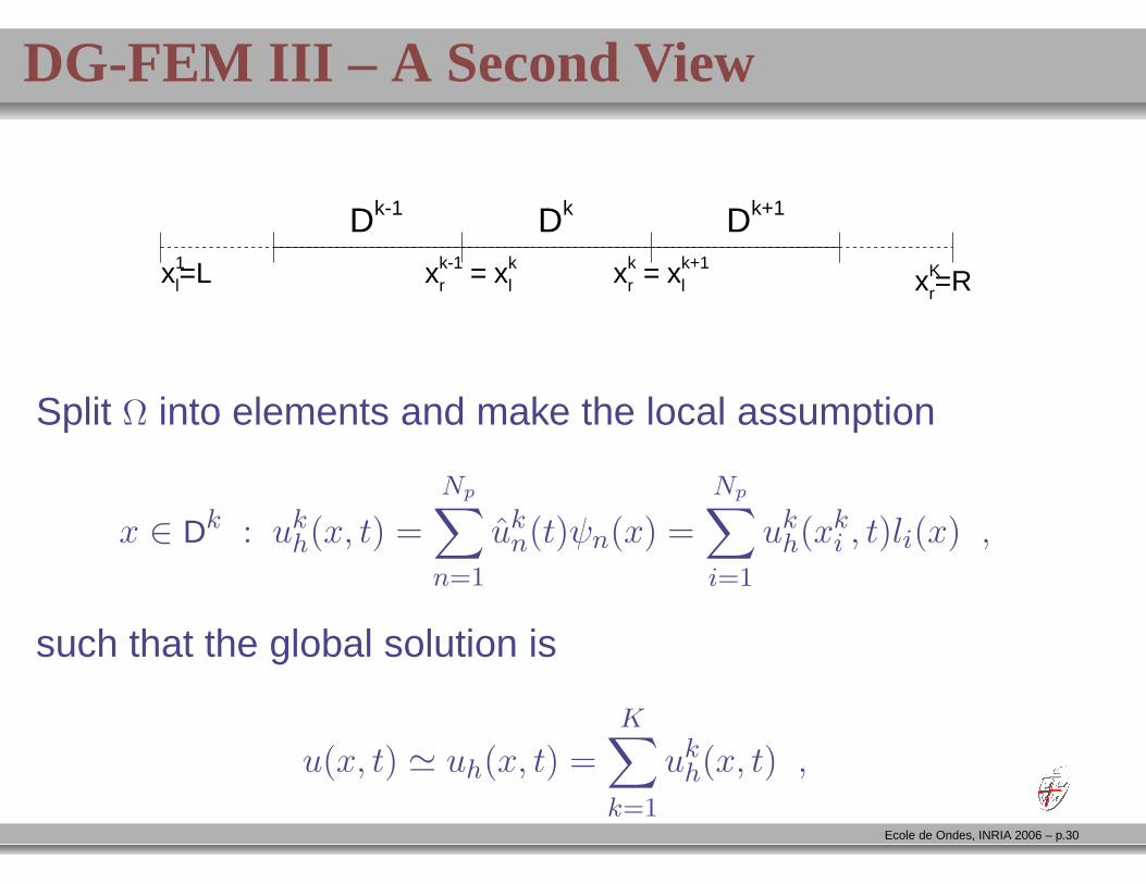
Split Ω into elements and make the local assumption

x ∈ Dk : ukh(x, t) =

Np∑

n=1

ukn(t)ψn(x) =

Np∑

i=1

ukh(xk

i , t)li(x) ,

such that the global solution is

u(x, t) ≃ uh(x, t) =K∑

k=1

ukh(x, t) ,


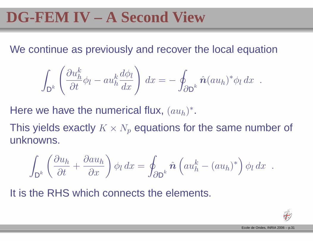
DG-FEM IV – A Second View

We continue as previously and recover the local equation

∫

Dk

(

∂ukh

∂tφl − auk

h

dφl

dx

)

dx = −

∮

∂Dkn(auh)∗φl dx .

Here we have the numerical flux, (auh)∗.

This yields exactly K ×Np equations for the same number ofunknowns.

∫

Dk

(

∂uh

∂t+∂auh

∂x

)

φl dx =

∮

∂Dkn(

aukh − (auh)∗

)

φl dx .

It is the RHS which connects the elements.


DG-FEM V – A Second View

In the standard form, φ(x) = ψ(x) and we obtain

Mk d

dtuk

h −(

Sk)T

aukh = − (auh)∗ψ|xk

r+ (auh)∗ψ|xk

l,

Mk d

dtuk

h + Skaukh =

(

aukh − (auh)∗

)

ψ

∣

∣

∣

xkr

−(

aukh − (auh)∗

)

ψ

∣

∣

∣

xkl

,

Mkij = (ψi, ψj)Dk , Sk

ij =

(

ψi,dψj

dx

)

Dk

,

are the local mass- and stiffness matrices, respectively.Furthermore, we have

ukh = [uk

1, . . . , ukNp

]T , ψ = [ψ1(x), . . . , ψNp(x)]T .


DG-FEM VI – A Second View

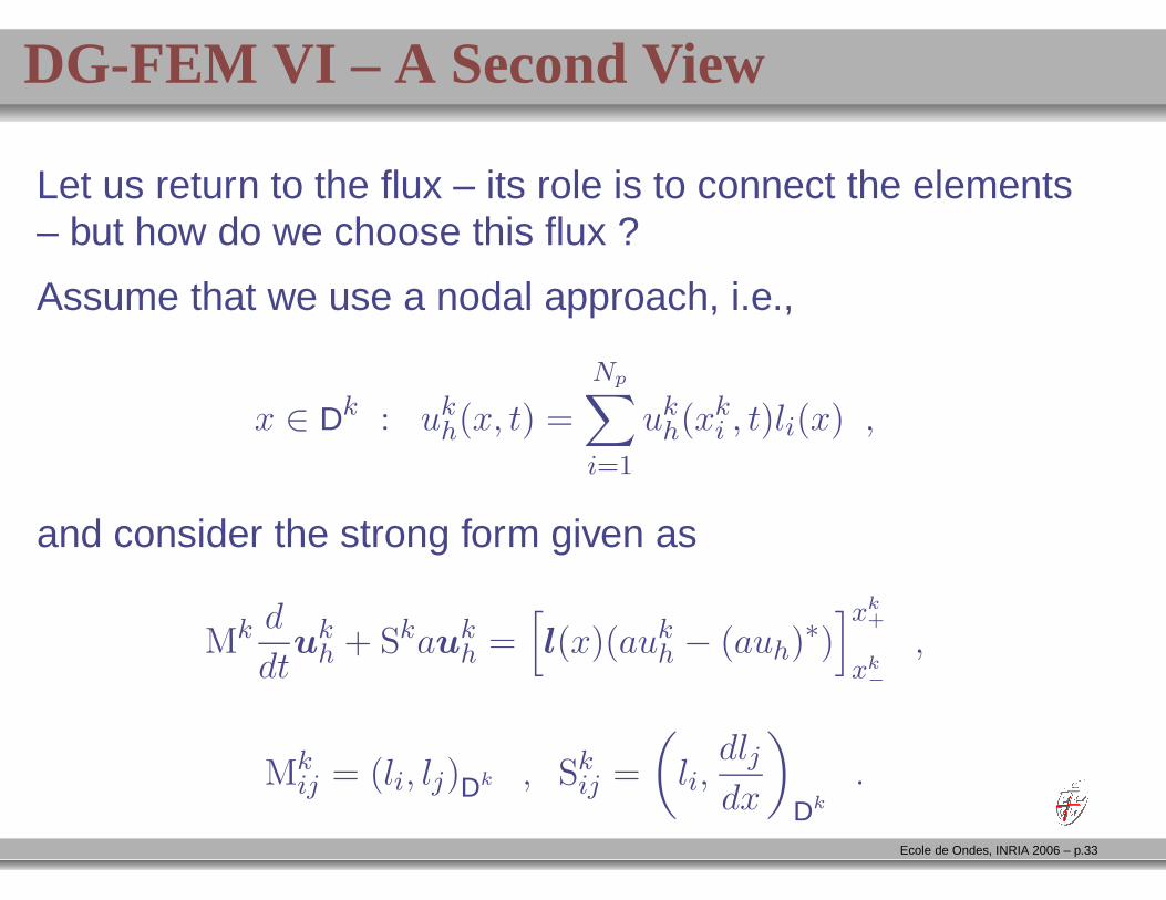
Let us return to the flux – its role is to connect the elements– but how do we choose this flux ?

Assume that we use a nodal approach, i.e.,

x ∈ Dk : ukh(x, t) =

Np∑

i=1

ukh(xk

i , t)li(x) ,

and consider the strong form given as

Mk d

dtuk

h + Skaukh =

[

l(x)(aukh − (auh)∗)

]xk+

xk−

,

Mkij = (li, lj)Dk , Sk

ij =

(

li,dlj

dx

)

Dk

.


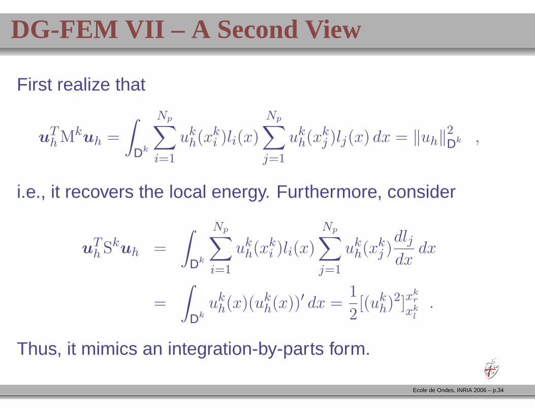
DG-FEM VII – A Second View

First realize that

uTh Mkuh =

∫

Dk

Np∑

i=1

ukh(xk

i )li(x)

Np∑

j=1

ukh(xk

j )lj(x) dx = ‖uh‖2Dk ,

i.e., it recovers the local energy. Furthermore, consider

uTh Skuh =

∫

Dk

Np∑

i=1

ukh(xk

i )li(x)

Np∑

j=1

ukh(xk

j )dlj

dxdx

=

∫

Dk

ukh(x)(uk

h(x))′ dx =1

2[(uk

h)2]xkr

xkl

.

Thus, it mimics an integration-by-parts form.


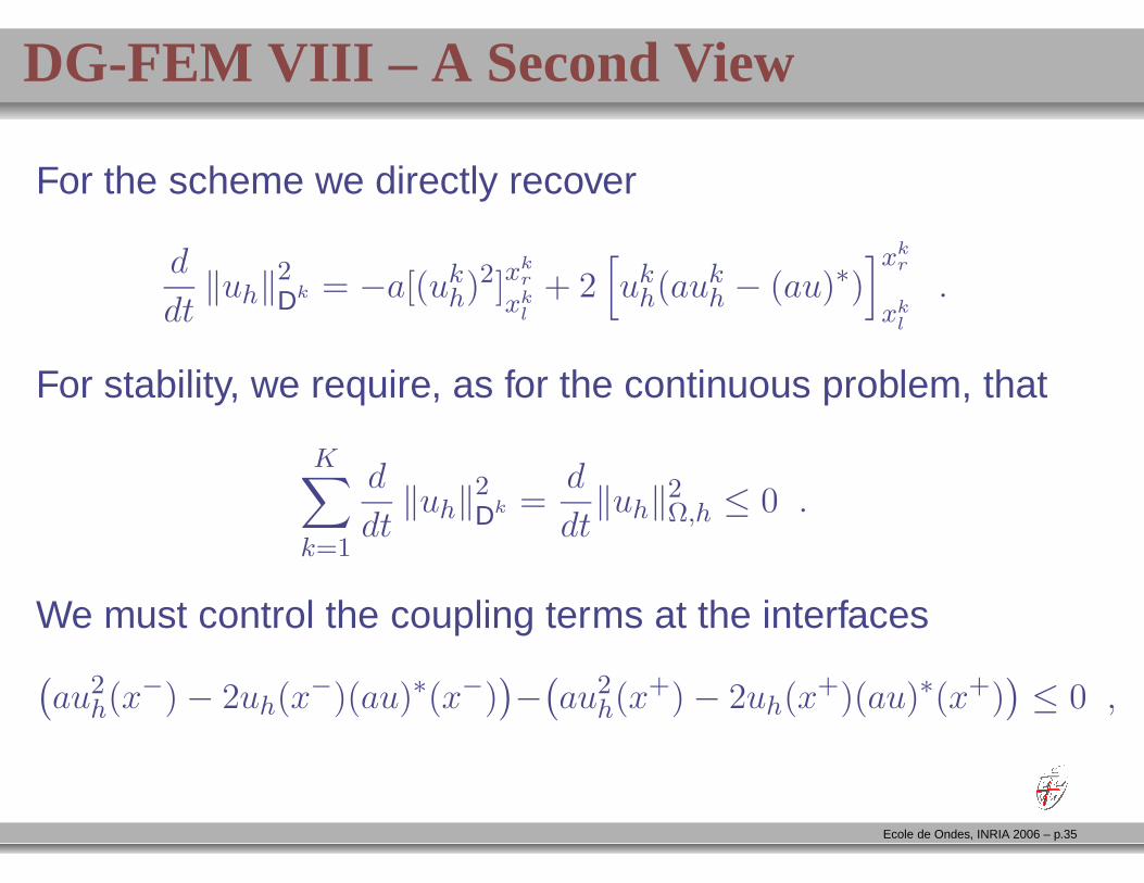
DG-FEM VIII – A Second View

For the scheme we directly recover

d

dt‖uh‖

2Dk = −a[(uk

h)2]xkr

xkl

+ 2[

ukh(auk

h − (au)∗)]xk

r

xkl

.

For stability, we require, as for the continuous problem, that

K∑

k=1

d

dt‖uh‖

2Dk =

d

dt‖uh‖

2Ω,h ≤ 0 .

We must control the coupling terms at the interfaces(

au2h(x−) − 2uh(x−)(au)∗(x−)

)

−(

au2h(x+) − 2uh(x+)(au)∗(x+)

)

≤ 0 ,


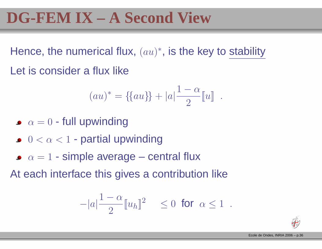
DG-FEM IX – A Second View

Hence, the numerical flux, (au)∗, is the key to stability

Let is consider a flux like

(au)∗ = au + |a|1 − α

2[[u]] .

α = 0 - full upwinding

0 < α < 1 - partial upwinding

α = 1 - simple average – central flux

At each interface this gives a contribution like

−|a|1 − α

2[[uh]]2 ≤ 0 for α ≤ 1 .


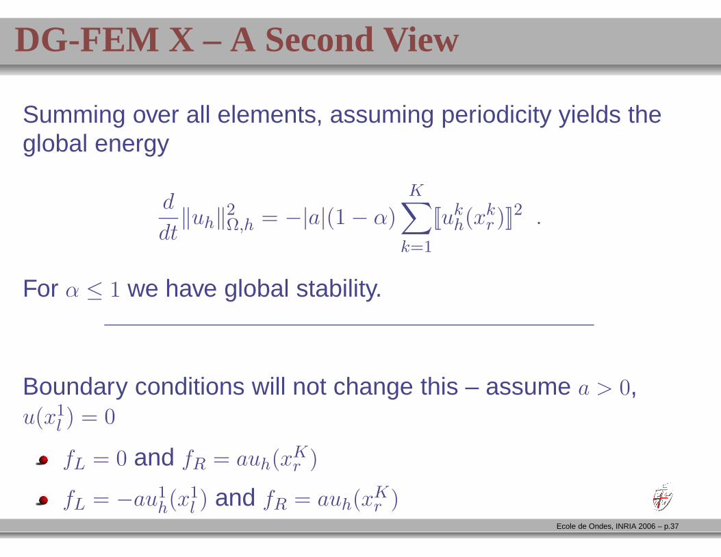
DG-FEM X – A Second View

Summing over all elements, assuming periodicity yields theglobal energy

d

dt‖uh‖

2Ω,h = −|a|(1 − α)

K∑

k=1

[[ukh(xk

r )]]2 .

For α ≤ 1 we have global stability.

Boundary conditions will not change this – assume a > 0,u(x1

l ) = 0

fL = 0 and fR = auh(xKr )

fL = −au1h(x1

l ) and fR = auh(xKr )


DG-FEM XI – A Second View

Thus, by choosing the flux, we can guarantee stability andeven energy conservation. Furthermore

The solutions are piecewise smooth, often polynomial,but discontinuous between elements.

Boundary conditions are enforced only weakly.

All operators are local.

But what about accuracy and convergence ?


DG-FEM XII – An Example

Let us consider an example

∂u

∂t− 2π

∂u

∂x= 0 , x ∈ [0, 2π] ,

u(0, t) = u(2π, t) , u(x, 0) = sin(lx) .

We solve this problem using the strong nodal form and a 4thorder ERK in time with a small timestep.

We would like to study 3 things

Accuracy dependence on h and N

Accuracy dependence on final time, T .

Computational cost


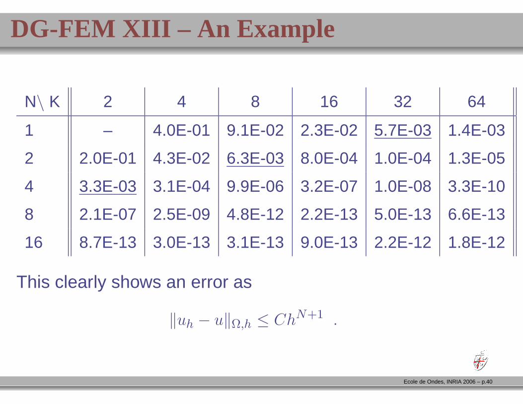
DG-FEM XIII – An Example

N\ K 2 4 8 16 32 64

1 – 4.0E-01 9.1E-02 2.3E-02 5.7E-03 1.4E-03

2 2.0E-01 4.3E-02 6.3E-03 8.0E-04 1.0E-04 1.3E-05

4 3.3E-03 3.1E-04 9.9E-06 3.2E-07 1.0E-08 3.3E-10

8 2.1E-07 2.5E-09 4.8E-12 2.2E-13 5.0E-13 6.6E-13

16 8.7E-13 3.0E-13 3.1E-13 9.0E-13 2.2E-12 1.8E-12

This clearly shows an error as

‖uh − u‖Ω,h ≤ ChN+1 .


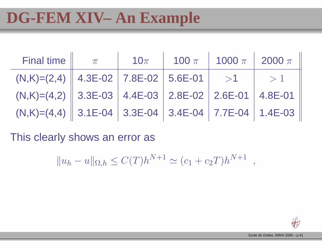
DG-FEM XIV– An Example

Final time π 10π 100 π 1000 π 2000 π

(N,K)=(2,4) 4.3E-02 7.8E-02 5.6E-01 >1 > 1

(N,K)=(4,2) 3.3E-03 4.4E-03 2.8E-02 2.6E-01 4.8E-01

(N,K)=(4,4) 3.1E-04 3.3E-04 3.4E-04 7.7E-04 1.4E-03

This clearly shows an error as

‖uh − u‖Ω,h ≤ C(T )hN+1 ≃ (c1 + c2T )hN+1 ,


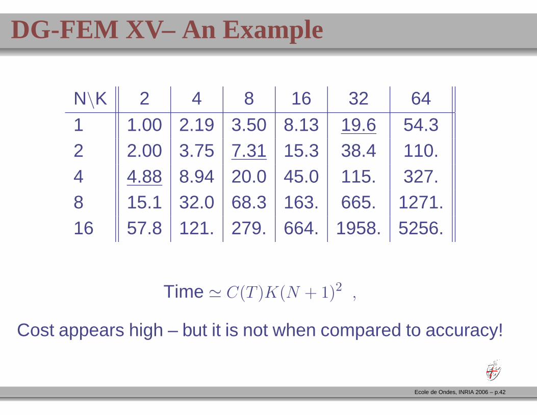
DG-FEM XV– An Example

N\K 2 4 8 16 32 64

1 1.00 2.19 3.50 8.13 19.6 54.32 2.00 3.75 7.31 15.3 38.4 110.4 4.88 8.94 20.0 45.0 115. 327.8 15.1 32.0 68.3 163. 665. 1271.16 57.8 121. 279. 664. 1958. 5256.

Time ≃ C(T )K(N + 1)2 ,

Cost appears high – but it is not when compared to accuracy!


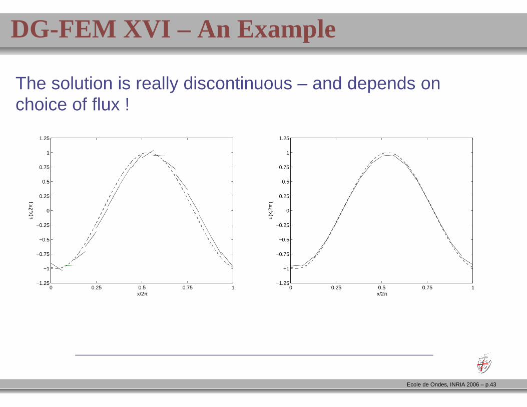
DG-FEM XVI – An Example

The solution is really discontinuous – and depends onchoice of flux !

0 0.25 0.5 0.75 1−1.25

−1

−0.75

−0.5

−0.25

0

0.25

0.5

0.75

1

1.25

x/2π

u(x,

2π )

0 0.25 0.5 0.75 1−1.25

−1

−0.75

−0.5

−0.25

0

0.25

0.5

0.75

1

1.25

x/2π

u(x,

2π )


A Brief Summary

The DG-FEM is a mixture of FE and FV methods

The local basis allows for high-order accuracy

The local statement of the PDE yields a local, explicitscheme

The numerical flux is key to ensuring stability

Boundary conditions are not satisfied exactly

. . . is it more memory intensive than FE

What about generalizations – systems, higher dimensions,

nonlinearities ?


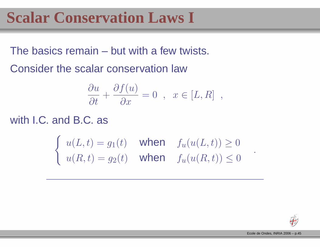
Scalar Conservation Laws I

The basics remain – but with a few twists.

Consider the scalar conservation law

∂u

∂t+∂f(u)

∂x= 0 , x ∈ [L,R] ,

with I.C. and B.C. as

u(L, t) = g1(t) when fu(u(L, t)) ≥ 0

u(R, t) = g2(t) when fu(u(R, t)) ≤ 0.


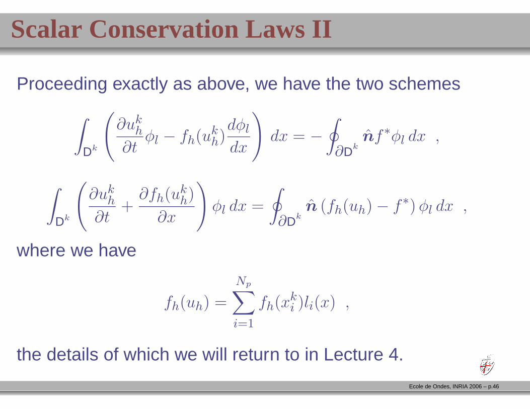
Scalar Conservation Laws II

Proceeding exactly as above, we have the two schemes

∫

Dk

(

∂ukh

∂tφl − fh(uk

h)dφl

dx

)

dx = −

∮

∂Dknf∗φl dx ,

∫

Dk

(

∂ukh

∂t+∂fh(uk

h)

∂x

)

φl dx =

∮

∂Dkn (fh(uh) − f∗)φl dx ,

where we have

fh(uh) =

Np∑

i=1

fh(xki )li(x) ,

the details of which we will return to in Lecture 4.


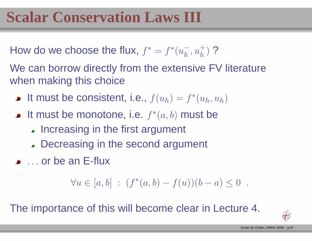
Scalar Conservation Laws III

How do we choose the flux, f∗ = f∗(u−h , u+h ) ?

We can borrow directly from the extensive FV literaturewhen making this choice

It must be consistent, i.e., f(uh) = f∗(uh, uh)

It must be monotone, i.e. f∗(a, b) must beIncreasing in the first argumentDecreasing in the second argument

. . . or be an E-flux

∀u ∈ [a, b] : (f∗(a, b) − f(u))(b− a) ≤ 0 .

The importance of this will become clear in Lecture 4.


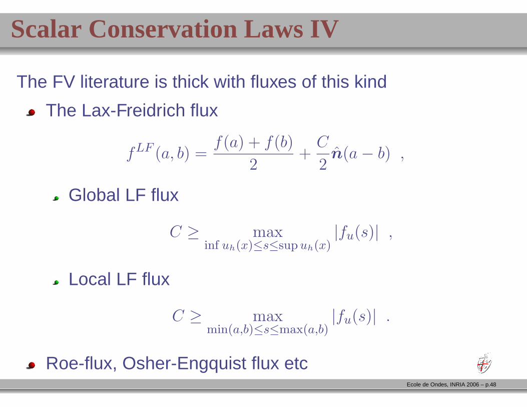
Scalar Conservation Laws IV

The FV literature is thick with fluxes of this kind

The Lax-Freidrich flux

fLF (a, b) =f(a) + f(b)

2+C

2n(a− b) ,

Global LF flux

C ≥ maxinf uh(x)≤s≤sup uh(x)

|fu(s)| ,

Local LF flux

C ≥ maxmin(a,b)≤s≤max(a,b)

|fu(s)| .

Roe-flux, Osher-Engquist flux etcEcole de Ondes, INRIA 2006 – p.48

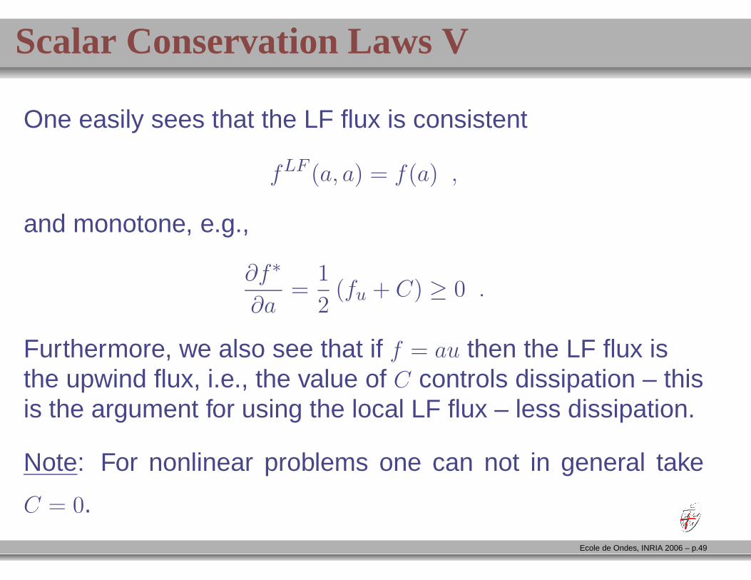
Scalar Conservation Laws V

One easily sees that the LF flux is consistent

fLF (a, a) = f(a) ,

and monotone, e.g.,

∂f∗

∂a=

1

2(fu + C) ≥ 0 .

Furthermore, we also see that if f = au then the LF flux isthe upwind flux, i.e., the value of C controls dissipation – thisis the argument for using the local LF flux – less dissipation.

Note: For nonlinear problems one can not in general take

C = 0.


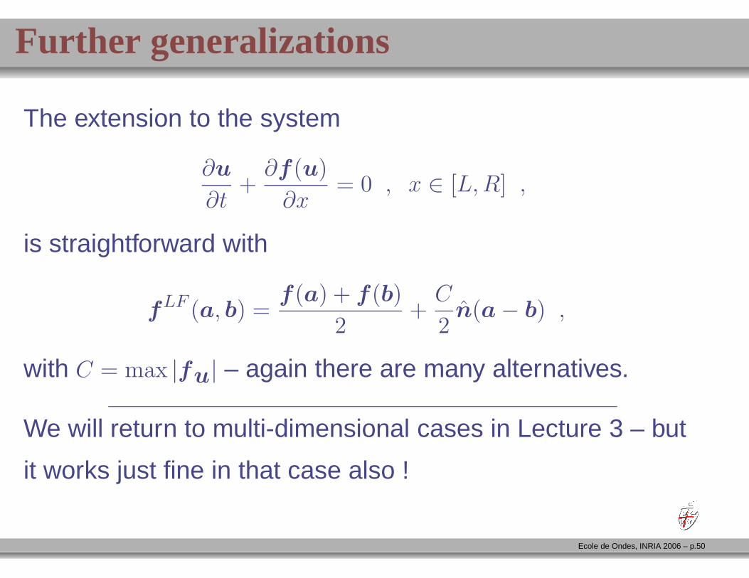
Further generalizations

The extension to the system

∂u

∂t+∂f(u)

∂x= 0 , x ∈ [L,R] ,

is straightforward with

fLF (a, b) =f(a) + f(b)

2+C

2n(a− b) ,

with C = max |fu| – again there are many alternatives.

We will return to multi-dimensional cases in Lecture 3 – but

it works just fine in that case also !


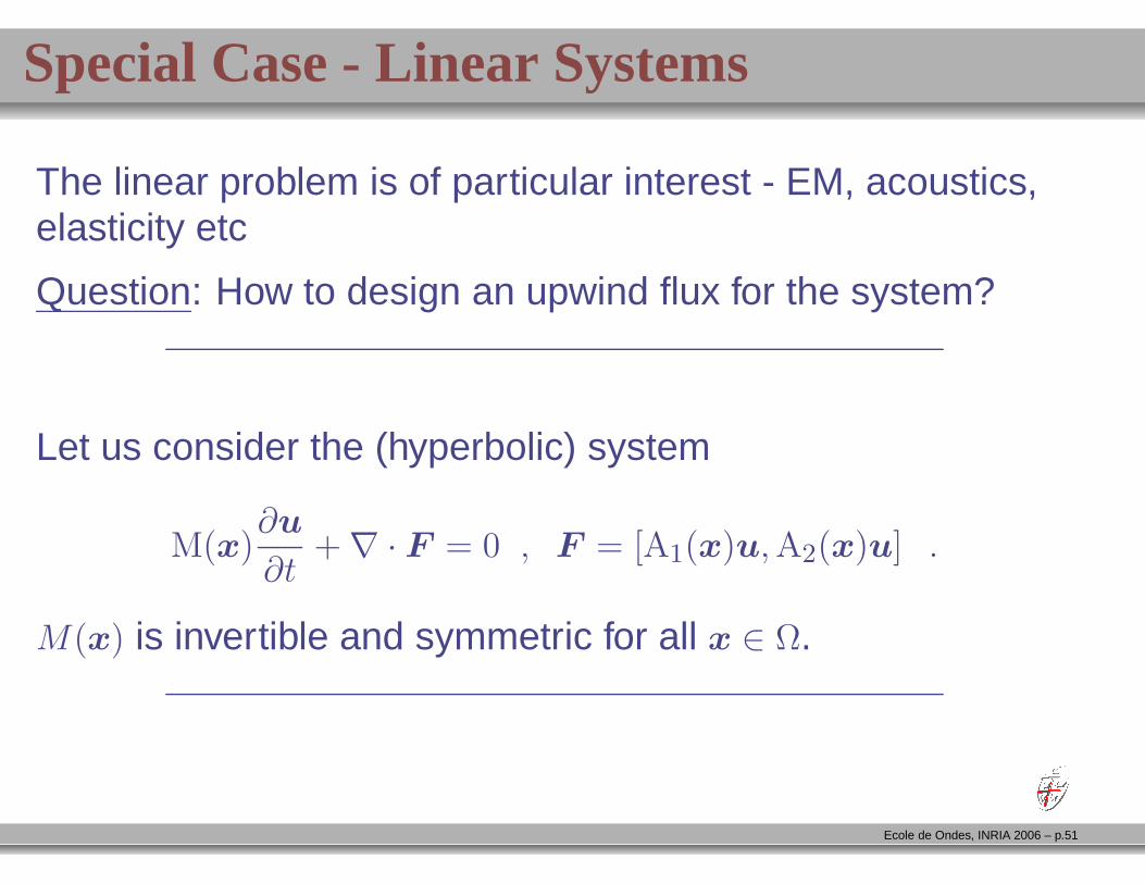
Special Case - Linear Systems

The linear problem is of particular interest - EM, acoustics,elasticity etc

Question: How to design an upwind flux for the system?

Let us consider the (hyperbolic) system

M(x)∂u

∂t+ ∇ · F = 0 , F = [A1(x)u,A2(x)u] .

M(x) is invertible and symmetric for all x ∈ Ω.


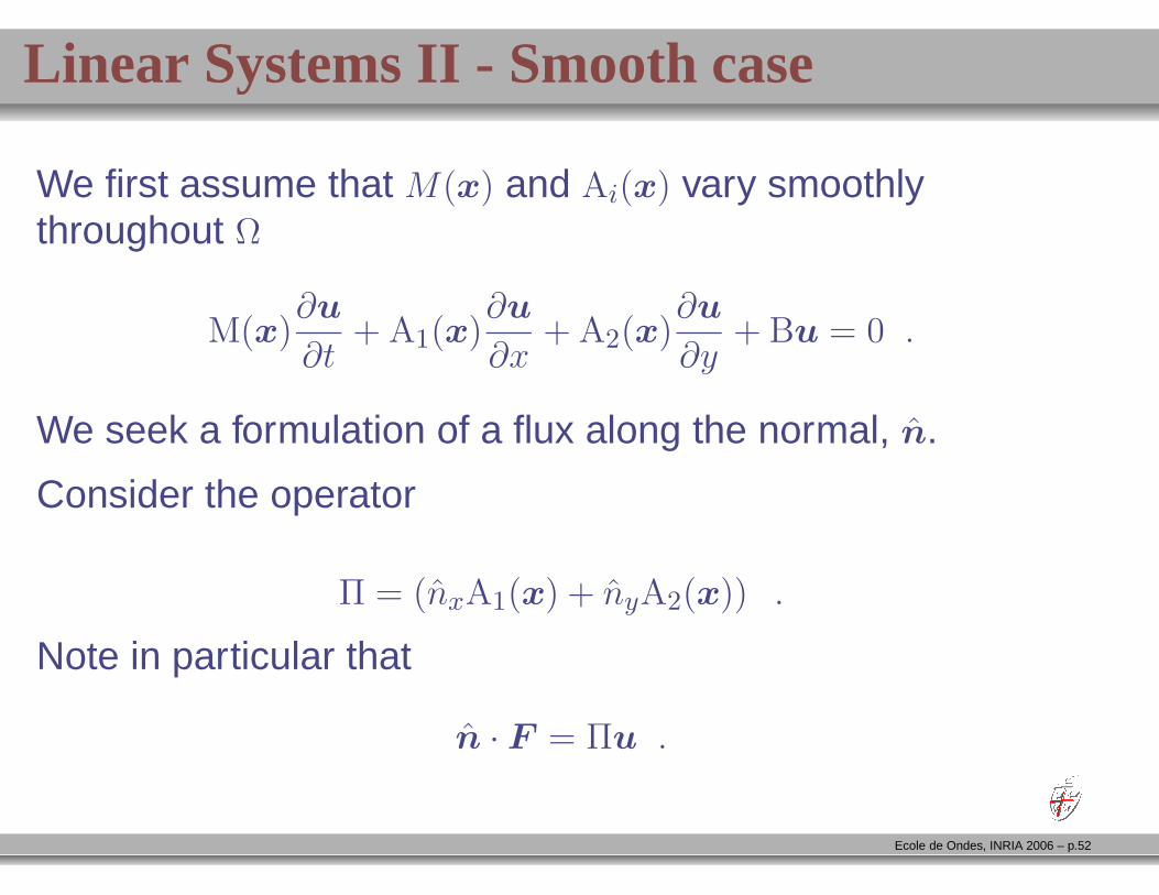
Linear Systems II - Smooth case

We first assume that M(x) and Ai(x) vary smoothlythroughout Ω

M(x)∂u

∂t+ A1(x)

∂u

∂x+ A2(x)

∂u

∂y+ Bu = 0 .

We seek a formulation of a flux along the normal, n.

Consider the operator

Π = (nxA1(x) + nyA2(x)) .

Note in particular that

n · F = Πu .


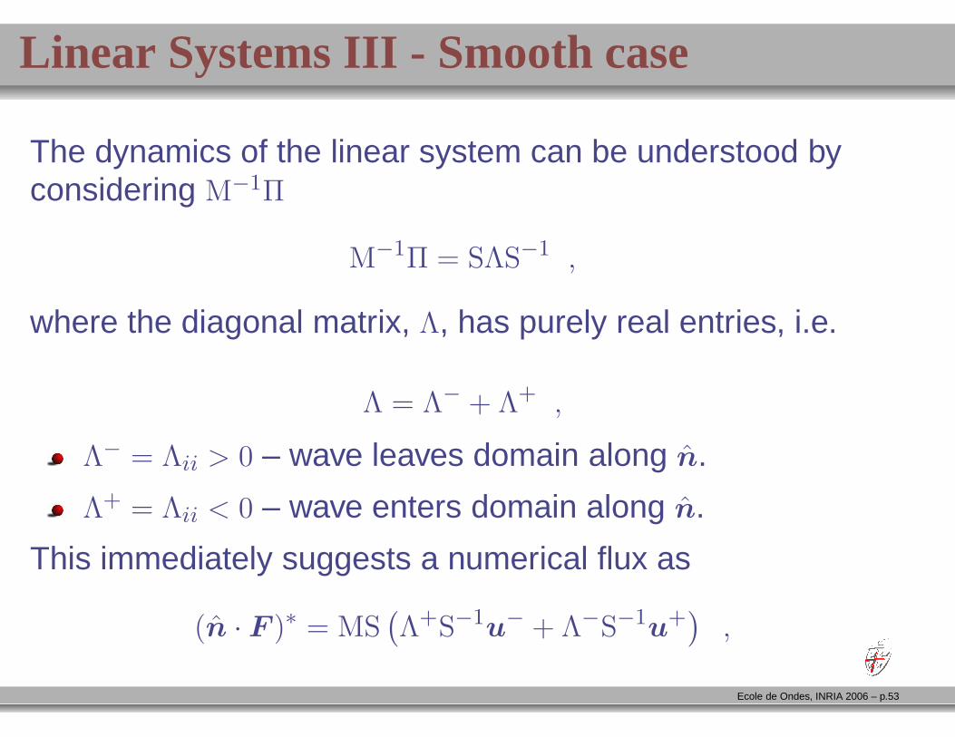
Linear Systems III - Smooth case

The dynamics of the linear system can be understood byconsidering M−1Π

M−1Π = SΛS−1 ,

where the diagonal matrix, Λ, has purely real entries, i.e.

Λ = Λ− + Λ+ ,

Λ− = Λii > 0 – wave leaves domain along n.

Λ+ = Λii < 0 – wave enters domain along n.

This immediately suggests a numerical flux as

(n · F )∗ = MS(

Λ+S−1u− + Λ−S−1u+)

,


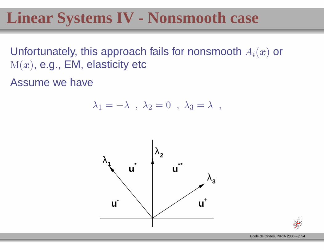
Linear Systems IV - Nonsmooth case

Unfortunately, this approach fails for nonsmooth Ai(x) orM(x), e.g., EM, elasticity etc

Assume we have

λ1 = −λ , λ2 = 0 , λ3 = λ ,

u-

u* u**

u+

λ1

λ2

λ3


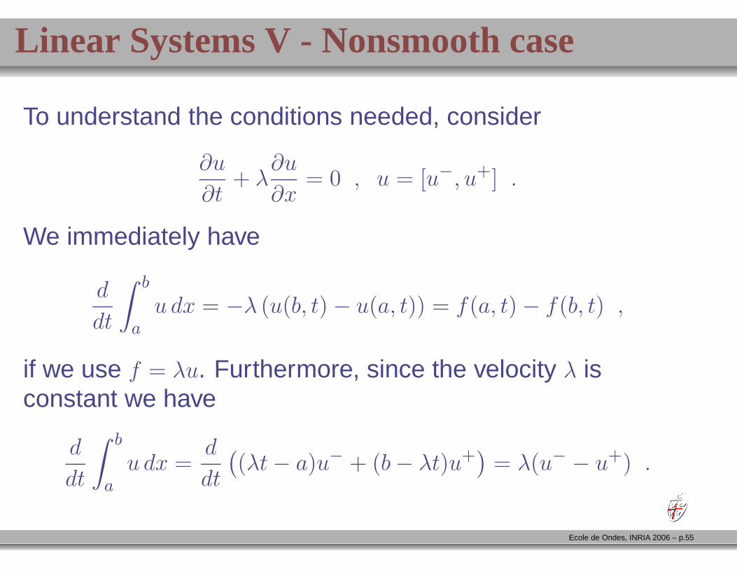
Linear Systems V - Nonsmooth case

To understand the conditions needed, consider

∂u

∂t+ λ

∂u

∂x= 0 , u = [u−, u+] .

We immediately have

d

dt

∫ b

au dx = −λ (u(b, t) − u(a, t)) = f(a, t) − f(b, t) ,

if we use f = λu. Furthermore, since the velocity λ isconstant we have

d

dt

∫ b

au dx =

d

dt

(

(λt− a)u− + (b− λt)u+)

= λ(u− − u+) .


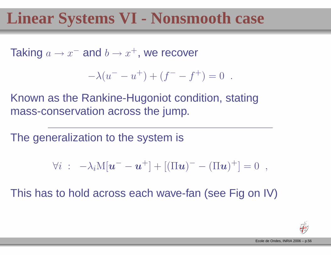
Linear Systems VI - Nonsmooth case

Taking a→ x− and b→ x+, we recover

−λ(u− − u+) + (f− − f+) = 0 .

Known as the Rankine-Hugoniot condition, statingmass-conservation across the jump.

The generalization to the system is

∀i : −λiM[u− − u+] + [(Πu)− − (Πu)+] = 0 ,

This has to hold across each wave-fan (see Fig on IV)


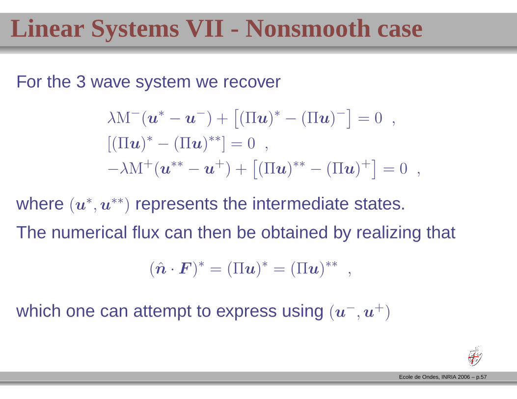
Linear Systems VII - Nonsmooth case

For the 3 wave system we recover

λM−(u∗ − u−) +[

(Πu)∗ − (Πu)−]

= 0 ,

[(Πu)∗ − (Πu)∗∗] = 0 ,

−λM+(u∗∗ − u+) +[

(Πu)∗∗ − (Πu)+]

= 0 ,

where (u∗,u∗∗) represents the intermediate states.

The numerical flux can then be obtained by realizing that

(n · F )∗ = (Πu)∗ = (Πu)∗∗ ,

which one can attempt to express using (u−,u+)


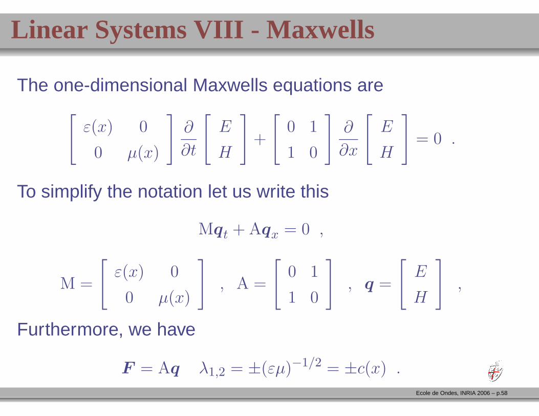
Linear Systems VIII - Maxwells

The one-dimensional Maxwells equations are[

ε(x) 0

0 µ(x)

]

∂

∂t

[

E

H

]

+

[

0 1

1 0

]

∂

∂x

[

E

H

]

= 0 .

To simplify the notation let us write this

Mqt + Aqx = 0 ,

M =

[

ε(x) 0

0 µ(x)

]

, A =

[

0 1

1 0

]

, q =

[

E

H

]

,

Furthermore, we have

F = Aq λ1,2 = ±(εµ)−1/2 = ±c(x) .


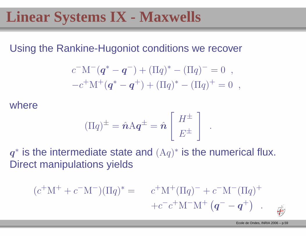
Linear Systems IX - Maxwells

Using the Rankine-Hugoniot conditions we recover

c−M−(q∗ − q−) + (Πq)∗ − (Πq)− = 0 ,

−c+M+(q∗ − q+) + (Πq)∗ − (Πq)+ = 0 ,

where

(Πq)± = nAq± = n

[

H±

E±

]

.

q∗ is the intermediate state and (Aq)∗ is the numerical flux.Direct manipulations yields

(c+M+ + c−M−)(Πq)∗ = c+M+(Πq)− + c−M−(Πq)+

+c−c+M−M+(

q− − q+)

.


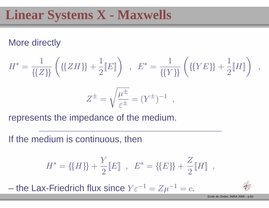
Linear Systems X - Maxwells

More directly

H∗ =1

Z

(

ZH +1

2[[E]]

)

, E∗ =1

Y

(

Y E +1

2[[H]]

)

,

Z± =

√

µ±

ε±= (Y ±)−1 ,

represents the impedance of the medium.

If the medium is continuous, then

H∗ = H +Y

2[[E]] , E∗ = E +

Z

2[[H]] ,

– the Lax-Friedrich flux since Y ε−1 = Zµ−1 = c.Ecole de Ondes, INRIA 2006 – p.60

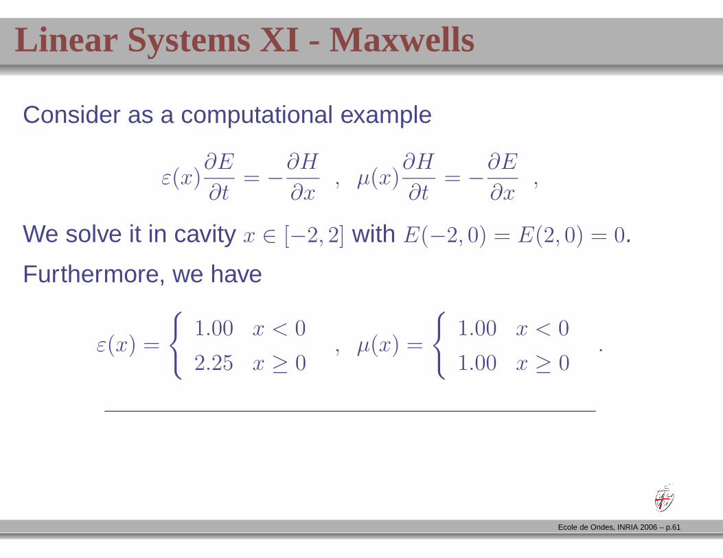
Linear Systems XI - Maxwells

Consider as a computational example

ε(x)∂E

∂t= −

∂H

∂x, µ(x)

∂H

∂t= −

∂E

∂x,

We solve it in cavity x ∈ [−2, 2] with E(−2, 0) = E(2, 0) = 0.

Furthermore, we have

ε(x) =

1.00 x < 0

2.25 x ≥ 0, µ(x) =

1.00 x < 0

1.00 x ≥ 0.


Linear Systems XII - Maxwells

Following the basic approach outlined previously, we recover

MkεdEk

h

dt+ SkHk

h =[

l(xk)(Hkh −H∗)

]xkr

xkl

,

MkµdHk

h

dt+ SkEk

h =[

l(xk)(Ekh − E∗)

]xkr

xkl

,

H∗ =1

Z

(

ZH +1

2[[E]]

)

, E∗ =1

Y

(

Y E +1

2[[H]]

)

,

H− −H∗ =1

2Z

(

n−Z+[[H]] − [[E]])

,

E− − E∗ =1

2Y

(

n−Y +[[E]] − [[H]])

.


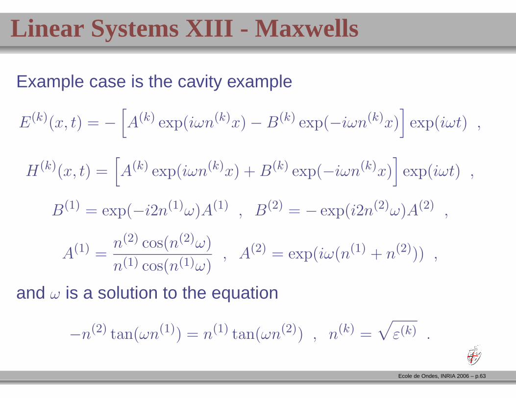
Linear Systems XIII - Maxwells

Example case is the cavity example

E(k)(x, t) = −[

A(k) exp(iωn(k)x) − B(k) exp(−iωn(k)x)]

exp(iωt) ,

H(k)(x, t) =[

A(k) exp(iωn(k)x) + B(k) exp(−iωn(k)x)]

exp(iωt) ,

B(1) = exp(−i2n(1)ω)A(1) , B(2) = − exp(i2n(2)ω)A(2) ,

A(1) =n(2) cos(n(2)ω)

n(1) cos(n(1)ω), A(2) = exp(iω(n(1) + n(2))) ,

and ω is a solution to the equation

−n(2) tan(ωn(1)) = n(1) tan(ωn(2)) , n(k) =√

ε(k) .


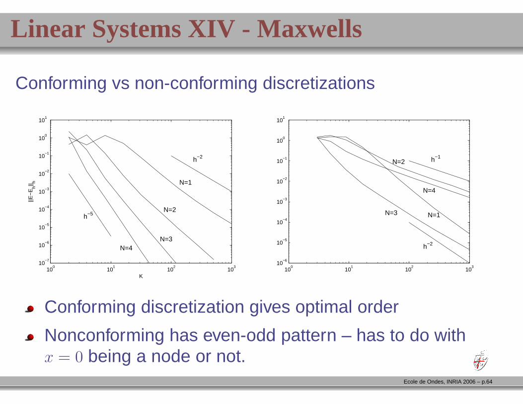
Linear Systems XIV - Maxwells

Conforming vs non-conforming discretizations

100

101

102

103

10−7

10−6

10−5

10−4

10−3

10−2

10−1

100

101

K

||E−

Eh|| h

h−2

h−5

N=1

N=2

N=3N=4

100

101

102

103

10−6

10−5

10−4

10−3

10−2

10−1

100

101

h−1

h−2

N=1

N=2

N=3

N=4

Conforming discretization gives optimal order

Nonconforming has even-odd pattern – has to do withx = 0 being a node or not.


Summary of Lecture 1

DG-FEM is a ’best-of-both’ mix of FV and FE

The local basis controls the accuracy of the scheme

N ’th order scheme appears to yield hN+1 accuracy

Stability is controlled by choice of the flux

For linear problems, both central and upwinding can bederived rigorously

For nonlinear problems, monotone fluxes are required

Can we prove these things ? – and what aboutimplementations ? – sit tight for Lecture 2 !


DG-FEM for Time-Dependent Problems Lecture 1: The Basics

Documents

Transcript of DG-FEM for Time-Dependent Problems Lecture 1: The Basics