January 2004 • NREL/SR-510-33524

Jacob Kaminsky Columbia, Maryland

Development of Strategies for Deployment of Biomass Resources in the Production of Biomass Power November 6, 2001 – February 28, 2003

National Renewable Energy Laboratory 1617 Cole Boulevard Golden, Colorado 80401-3393 NREL is a U.S. Department of Energy Laboratory Operated by Midwest Research Institute • Battelle

Contract No. DE-AC36-99-GO10337

January 2004 • NREL/SR-510-33524

Development of Strategies for Deployment of Biomass Resources in the Production of Biomass Power November 6, 2001 – February 28, 2003

Jacob Kaminsky Columbia, Maryland

NREL Technical Monitor: L. Wentworth Prepared under Subcontract No. LAR-2-31121-01

National Renewable Energy Laboratory 1617 Cole Boulevard Golden, Colorado 80401-3393 NREL is a U.S. Department of Energy Laboratory Operated by Midwest Research Institute • Battelle

Contract No. DE-AC36-99-GO10337

This publication was reproduced from the best available copy

Submitted by the subcontractor and received no editorial review at NREL NOTICE This report was prepared as an account of work sponsored by an agency of the United States government. Neither the United States government nor any agency thereof, nor any of their employees, makes any warranty, express or implied, or assumes any legal liability or responsibility for the accuracy, completeness, or usefulness of any information, apparatus, product, or process disclosed, or represents that its use would not infringe privately owned rights. Reference herein to any specific commercial product, process, or service by trade name, trademark, manufacturer, or otherwise does not necessarily constitute or imply its endorsement, recommendation, or favoring by the United States government or any agency thereof. The views and opinions of authors expressed herein do not necessarily state or reflect those of the United States government or any agency thereof.

Available electronically at http://www.osti.gov/bridge

Available for a processing fee to U.S. Department of Energy and its contractors, in paper, from:

U.S. Department of Energy Office of Scientific and Technical Information P.O. Box 62 Oak Ridge, TN 37831-0062 phone: 865.576.8401 fax: 865.576.5728 email: reports@adonis.osti.gov

Available for sale to the public, in paper, from:

U.S. Department of Commerce National Technical Information Service 5285 Port Royal Road Springfield, VA 22161 phone: 800.553.6847 fax: 703.605.6900 email: orders@ntis.fedworld.gov online ordering: http://www.ntis.gov/ordering.htm

Printed on paper containing at least 50% wastepaper, including 20% postconsumer waste

1

Overview

Biopower, the production of electricity from biomass, is one of the most promising

alternatives to the production of electricity from fossil fuels. According to the Energy

Information Administration (EIA) Energy Outlook 2002, of the renewable energy resources

under development, wind and biomass have the greatest potential to penetrate the electric

market in the next twenty years. Although a variety of programs and incentives have been

deployed in the past, the market for new biopower has been limited. A key reason for the

lack of biopower growth has been the limited availability of biomass at a price competitive

with coal.

Many studies have been undertaken to assess the impact of alternative policy scenarios on

biopower potential. In this study several of the projections made in the last two years were

selected for evaluation: the Energy Information Administration (EIA), Oak Ridge National

Laboratory (ORNL), OnLocation Inc., and ICF Inc. Three models were used in these

projections: the National Energy Modeling System (NEMS), the Oak Ridge Competitive

Electricity Dispatch (ORCED) model, and the Integrated Planning Model (IPM). The

projections included several national projections and the ORNL Southeast Study projections.

Projections were made for four scenarios: Base or Reference Case, Unlimited Resources,

Renewable Portfolio Standards (RPS), and Environmental Impact Standards. Several options

were projected under each scenario. In total, projections were made for over 27 options.

The study analyzes strategies for deployment of biomass resources for Biopower generation. It evaluates and compares several biomass supply databases. It also compares the projected biopower market penetration for several alternative incentive scenarios. It analyzes the availability of biomass to meet the projected market demands. Based on the analysis, a summary of findings and recommended future research is presented.

2

The study compared and evaluated the basic assumptions, the inputs to the projections, and

the projection results. For each scenario the study a) compared market penetration among

the models, b) evaluated the reason for variation of results between the models, c) compared

the results and identified the variation of results in the different regions, and d) analyzed the

market potential and the impact on the prices that power plants would pay for biomass under

the alternative projections.

The economic viability of biopower is dependent in part on the cost and availability of

biomass. Biomass prices for biopower vary by the type of biomass and by the distance of the

biomass from the power plant. There are two major biomass categories: biomass residues

and energy crops. Four types of biomass residues are used as fuel for generating electricity

including, agricultural residues, forest residues, mill residues and urban wood waste. Energy

crops are plants that are grown solely for the use of energy production. The energy crops are

divided into two types: grasses and short rotation woody (SRW) crops. The quantities of

available biomass were estimated by the biomass type and price. Three biomass supply

databases were reviewed, one developed by NEMS and two developed by ORNL.

Biopower’s potential market is dependent in part on the availability of biomass at a price

competitive with coal. Each projection was evaluated to determine a) the quantities of

resources needed to meet the demand, b) the competitive price that power plants could pay

for biomass, c) the availability of adequate resources to meet the demand at the competitive

price, d) the types of resources that were available to meet the biomass demand, e) the

resource price that would ensure the availability of adequate resources to meet the demand.

The availability of resources, the type of resources, and the price of resources that would be

required to meet the projected markets were determined for each alternative policy.

The report is divided into six chapters. Chapter One presents a summary of findings and

recommendations for future research. Chapter Two describes the models used in the

3

projections. Chapter Three describes and compares the results of the national projections.

Chapter Four describes and compares the biomass resource databases used in the projections.

Chapter Five analyzes the national projections with resource availability. In Chapter Six the

Southeast Regional Study projections are analyzed.

4

Contributions

The report is based on studies, publications, databases, discussions, and input from several agencies and individuals. Thanks and gratitude are extended to the following: Lynn Wright, Marie Walsh, Bob Perlack, Stan Hadley, Jim Van Dyke and Shahab Sokhansani - ORNL Zia Hag – EIA Juanita Haydel and Thapa Bishal - ICF Frances Wood – OnLocation Larry Goldstein – NREL Kevin Comer and Edward Gray – Antares Selected memos or reports prepared by the individuals are included in the appendices. There will not be specific credit notations in the body of the report. Reports from which information was used in the study are: Biomass for Electricity Generation, http://www.eia.doe.gov/oiaf/analysispaper/index.html Zia Hag, EIA, DOE Annual Energy Outlook 2002 http://www.eia.doe.gov/oiaf/aeo/index.html ICF Memorandum: Potential Market Penetration of Biomass Co-firing, Interim Report - January 31, 2001 ICF Memorandum: Results of Phase II of Study on Potential Market Penetration of Biomass Co-firing – July 19, 2001 NREL Memorandum: Biomass Cofiring Use at $20/Dry Ton. S. W. Hadley, 11/10/2000 NREL Memorandum: Biomass Cofiring Use at $20/Dry Ton with 15% Maximum. S. W. Hadley, 2/23/2001 Alternative Biomass Cofiring Scenarios Using NEMS, Prepared by OnLocation Inc., for the National Renewable Energy Laboratory, December 2000. Data received from Marie Walsh and Bob Perlock on ORNL Supply Curves and the Southeast Study and Zia Hag, EIA on NEMS Supply Curves and the RPS Projections Evaluation of Analysis Needs (Modeling and Data) for the BioPower Program, Prepared for Oak Ridge National Laboratory by the Antares Group, Incorporated, August 2001 Engineering Aspects of Collecting Corn Stover for Bioenergy, Shahab Sokhansanj, Anthony Turhollow, Janet Cushman, John Cundiff, Oak Ridge National Laboratory, 2001 Baseline Cost for Corn Stover Collection, Shahab Sokhansanj and Anthony Turhollow, Oak Ridge National Laboratory, May 2001

5

Table of Contents Overview………………………………………………………………………………………………….. 1 Summary of Findings and Recommended Research ........................................................................….. 6

Summary of Findings ................................................................................................................................ 6 Recommendations for future research..................................................................................................... 12

Models……………. ................................................................................................................................... 16 Model Descriptions ................................................................................................................................. 16 Comparison of Regions used by the models ........................................................................................... 18

Projections - Projection Scenarios, Input Assumptions and Projection Results................................. 21 Projection Scenarios ................................................................................................................................ 21 Unlimited Resources ............................................................................................................................... 22 Renewable Portfolio Standards Scenario ................................................................................................ 28 Environmental Impact Standards Scenario ............................................................................................. 29

Resources…………………………………………………………………………………………………31 Resource Types ....................................................................................................................................... 31 NEMS Supply Curves ............................................................................................................................. 33 Comparison of the NEMS and ORNL Supply Curves............................................................................ 39 Comparison of NEMS and ORNL Supply Estimates by Region ............................................................ 42

Analysis - Comparison of Resource Availability with Projected Market Demand............................. 44 Comparison of resource used and total resource availability .................................................................. 44 Comparison of Projected Biomass Used with Biomass Availability by Price Category ........................ 45 Comparison of Supply and Projected Demand for the Unlimited Resources Scenario .......................... 46 Renewable Portfolio Standards ............................................................................................................... 48 RPS Demand and Supply Analysis by Resource Type ........................................................................... 51

Southeast Region Study............................................................................................................................ 53 SES Supply Estimates ............................................................................................................................. 53 Comparison of Resource Estimates for the Southeast Region ................................................................ 54 Comparison between SES and NEMS Supply Curves by Price Categories............................................ 55 Projected Market Penetration .................................................................................................................. 58 Comparison with RPS Projections .......................................................................................................... 60

Appendix 1 - Biomass Cofiring Use at $20/dry ton................................................................................... 61 Appendix 2 - Biomass Cofiring Use at $20/dry ton with 15% Maximum................................................. 64 Appendix 3 - Potential Market Penetration of Biomass Co-firing, Interim Report ................................... 67 Appendix 4 - Results of Phase II of Study on Potential Market Penetration of Biomass Co-firing .......... 79

6

Summary of Findings and Recommended Research

Summary of Findings

Incentives

A combination of incentives that include Renewable Portfolio Standards (RPS) for biopower,

Environmental Impact Standards (EIS) for the electric generation industry, and agriculture

policies that encourage the use of biomass from CRP land would insure the competitiveness

of biopower in the market place. The incentives need to be high enough to enable power

producers to pay at least twice the current competitive price with coal for biomass. If the

incentive would allow the price for biomass to be twice the current biomass competitive price

of coal, the market potential will double over the Reference Case, in which no incentive is

applied. If the incentives would allow power plants to pay triple the competitive price of

coal for biomass, the market would quadruple, and if the price were four times the

competitive price of coal, the market would increase ten-fold.

The Renewable Portfolio Standards options tested are large enough to make an impact on

biopower market penetration. If the standards are mandated there will be more than adequate

resources to meet the demand. Under the RPS requirements, the biomass value is equivalent

to more than three times the current competitive biomass price of $20/ton.

The combined value of the two incentives, if applied only to the biomass price, would enable

utilities to pay as much as four times the current competitive price of coal.

Based on the three-cent penalty assumed by the RPS projections, the incentive value of the

RPS is $46-$50/ton. Based on the Southeast Study model calculation of the maximum price

paid for resources, the Low Carbon option incentive value is $18-$29/ton and the High

Carbon value is $29-$30/ton.

7

Most of the market for biopower is concentrated in the Southeast (SERC/STV) and Mid-

Atlantic (ECAR and MAIN) regions. Most projections predict that these three regions would

account for 50%-70% of the 2020 biopower market.

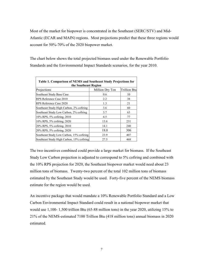
The chart below shows the total projected biomass used under the Renewable Portfolio

Standards and the Environmental Impact Standards scenarios, for the year 2010.

Table 1. Comparison of NEMS and Southeast Study Projections for the Southeast Region

Projections Million Dry Ton Trillion BtuSoutheast Study Base Case 0.6 10 RPS Reference Case 2010 2.2 38 RPS Reference Case 2020 1.3 21 Southeast Study High Carbon, 2% cofiring 3.6 60 Southeast Study Low Carbon, 2% cofiring 3.7 63 10% RPS, 5% cofiring, 2010 4.5 77 10% RPS, 5% cofiring, 2020 13.6 231 20% RPS, 5% cofiring, 2010 14.1 240 20% RPS, 5% cofiring, 2020 18.0 306 Southeast Study Low Carbon, 15% cofiring 23.9 407 Southeast Study High Carbon, 15% cofiring 27.5 468

The two incentives combined could provide a large market for biomass. If the Southeast

Study Low Carbon projection is adjusted to correspond to 5% cofiring and combined with

the 10% RPS projection for 2020, the Southeast biopower market would need about 23

million tons of biomass. Twenty-two percent of the total 102 million tons of biomass

estimated by the Southeast Study would be used. Forty-five percent of the NEMS biomass

estimate for the region would be used.

An incentive package that would mandate a 10% Renewable Portfolio Standard and a Low

Carbon Environmental Impact Standard could result in a national biopower market that

would use 1,100- 1,500 trillion Btu (65-88 million tons) in the year 2020, utilizing 15% to

21% of the NEMS-estimated 7100 Trillion Btu (418 million tons) annual biomass in 2020

estimated.

8

Resource Availability to Meet Projected Demand

If Renewable Portfolio Standards and Environmental Impact Standards were enacted, market

penetration could be limited by the availability of resources. Incentives that would allow

power producers to pay less than $40/dry ton will not have a significant impact on biopower

market penetration because there aren’t enough biomass resources at prices below $40/dry

ton.

All of the available resources, estimated by NEMS supply curves, at $20/dry ton are from

urban wood waste. The availability of these resources is questionable for several reasons: a)

a very low cost was assumed for processing, b) communities in urban areas oppose the use of

biomass for biopower because of traffic, noise and aesthetics, c) the spatial location of the

resources relative to the location of power plants limits the resources to a small number of

plants in any given region, and d) the cost and availability of land for biomass storage for

power plants in urban areas is a limiting factor.

The NEMS resource estimates at $30/dry ton are comprised of 75% urban wood waste and

25% forest residues. The quantities are also overestimated at this price for the same reasons

listed in the previous paragraph.

At $40/dry ton, the resource availability is comprised of 43% agriculture residues and 30%

forest residues. The Southeast Study suggests that the availability of agriculture residues in

the NEMS supply curves may be overestimated. The Southeast Study estimates for

agriculture residues in the SERC/STV are 95% lower than the ORNL national supply curve

estimates.

There are adequate quantities of biomass at $50/dry ton to meet most projections.

9

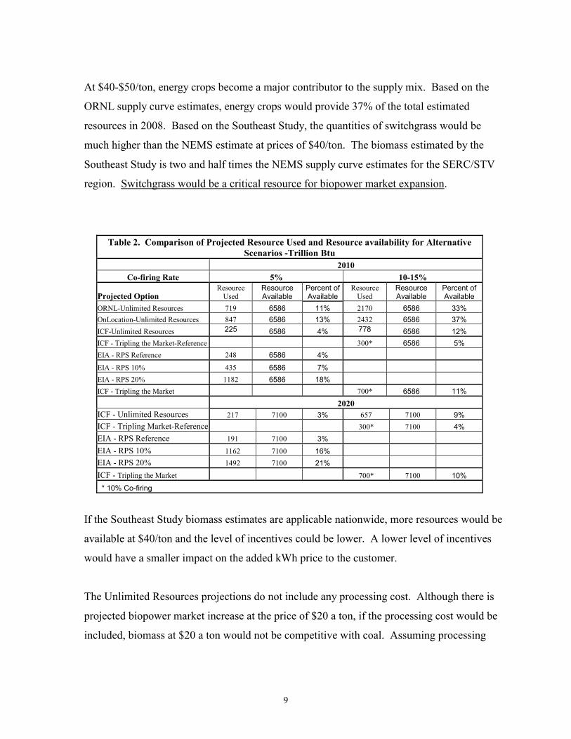
At $40-$50/ton, energy crops become a major contributor to the supply mix. Based on the

ORNL supply curve estimates, energy crops would provide 37% of the total estimated

resources in 2008. Based on the Southeast Study, the quantities of switchgrass would be

much higher than the NEMS estimate at prices of $40/ton. The biomass estimated by the

Southeast Study is two and half times the NEMS supply curve estimates for the SERC/STV

region. Switchgrass would be a critical resource for biopower market expansion.

Table 2. Comparison of Projected Resource Used and Resource availability for Alternative Scenarios -Trillion Btu

2010 Co-firing Rate 5% 10-15%

Projected Option Resource

Used Resource Available

Percent of Available

Resource Used

Resource Available

Percent of Available

ORNL-Unlimited Resources 719 6586 11% 2170 6586 33% OnLocation-Unlimited Resources 847 6586 13% 2432 6586 37% ICF-Unlimited Resources 225 6586 4% 778 6586 12% ICF - Tripling the Market-Reference 300* 6586 5% EIA - RPS Reference 248 6586 4% EIA - RPS 10% 435 6586 7% EIA - RPS 20% 1182 6586 18% ICF - Tripling the Market 700* 6586 11% 2020 ICF - Unlimited Resources 217 7100 3% 657 7100 9% ICF - Tripling Market-Reference 300* 7100 4% EIA - RPS Reference 191 7100 3% EIA - RPS 10% 1162 7100 16% EIA - RPS 20% 1492 7100 21% ICF - Tripling the Market 700* 7100 10% * 10% Co-firing

If the Southeast Study biomass estimates are applicable nationwide, more resources would be

available at $40/ton and the level of incentives could be lower. A lower level of incentives

would have a smaller impact on the added kWh price to the customer.

The Unlimited Resources projections do not include any processing cost. Although there is

projected biopower market increase at the price of $20 a ton, if the processing cost would be

included, biomass at $20 a ton would not be competitive with coal. Assuming processing

10

cost of at least $5-10 a ton biomass competitive price with coal would be $10-15 a ton. If the

heat loss and operation and management cost is added the competitive price with coal,

without incentives, at the power plant gate, is even smaller.

If utilities could pay $20-30 a ton for biomass, biopower market expansion would be limited

to cofiring in regions where coal prices are high and SO2 mitigation is at premium.

Biomass Supply Estimates

The cost of processing; cleaning, drying, grinding, densification, loading and moving, and

storage, is either under estimated or not included at all in the biomass supply curves. If the

complete cost of processing would be included in the supply curves, biomass quantities at the

lower price range of $20-40 per dry tons will decrease substantially.

The projections assume that all the estimated biomass resources are available exclusively for

Biopower use. If Biofuels would have similar incentives, and or industry would have

increased demand for biomass products the resource availability for biopower would be

smaller and the market penetration, at the lower biomass price categories, would be smaller.

Because of the uncertainty, in term of cost and availability, of both Agriculture Residues and

Forest Residues, the future for biopower without Energy Crops would be limited.

To have biomass for biopower utilities would have to pay about $50 a ton. Since each region

has a different predominant residue type, at $50 a ton, the combination of at least one residue

type with energy crop would be needed to insure availability of reliable biomass resources to

all plants in that region.

Each region has a different combination of resource types. The level of competition for

resources among users would depend on the resource types composition and the type of

resources each user would require. For example, if Agriculture residues and switchgrass

11

would be the main resources used by Biofuels and Biopower, there would be competition for

these resources in the ECAR and MAIN regions. In these regions there may not be adequate

resources to meet the demand for both.

The majority of resources at $40 are from Agriculture Residues. There is a debate as to the

quantities of Agriculture Residues that could be removed from the field. A simple

calculation suggests that if the farmer’s income is $10 a ton, the cost of collection is $20 a

ton (based on Shahab Sokhansani estimates), the transportation cost to the plant is $10 a ton,

and the processing and storage cost at the plant is $5 a ton, the total cost would average $45 a

ton.

Models Capability

The NEMS and ORCED models could complement each others capabilities to project market

potential for biopower. A major deficiency of the NEMS model is the assumption that total

resources in a region are available to all power plants in that region and transportation cost is

a fixed $10 a ton. The ORCED model, deficiency is that it does not have algorithms to

predict changes over time but only provide a snap shot of a given time. The ORCED model,

in combination with other ORNL models, can project biopower market based on the

availability of resources for each individual plant and calculate transportation cost for each

plant based on the resource distance from the plant. The two models could be used together

or in sequence. The NEMS model would be used to project the future number and location

of power plants for any region for any given year. The output would than be used by the

ORCED model to project and compare with the NEMS results, the potential for any given

region.

12

Recommendations for Future Research

Biopower Market Projection assuming both the RPS and the Low Carbon standards.

Biopower Market Projection using the three models, NEMS, ORCED and IPM, under

identical assumptions, that would include the two incentives, a 10% RPS and a Low Carbon,

is recommended to estimate the probable biopower market potential. The recommended

projections with the IPM model would be useful for comparison with NEMS projections and

for dialogue and communication between DOE and EPA.

Economic analysis of alternative sets of incentives. The study was limited to the analysis of

the projected biopower potential and biomass availability for selected scenarios. It did not

include an economic analysis. The economic impact of different combination of Renewable

Portfolio Standards, Environmental Impact Standards and CRP policies and incentives

should be analyzed. The economic analysis should be comprehensive and include impact on

consumer electric prices, environmental benefits and economic impact on the rural

economy. The result of such study would help draft an incentive program and provide a

background paper that would explain the reasoning for any recommended incentive package

for biopower.

Processing and Transport Infrastructure Systems. All the models assume that processing, or

converting the raw wood to a form appropriate for firing, is done at the power plant site. It

would be more economical and efficient for utilities to purchase biomass in a form ready to

be fed into the boiler and not be involved in the processing of biomass. Concepts of resource

collection, processing and distribution systems between the farm or resources collection gate

and the power plant should be explored and evaluated. For example, a system in which a

multi-purpose processing center is located along railroad tracks, where the railroad would be

used for biomass transport. The centers would collect all waste wood in the area, would

prepare the biomass in according to each user needs, and deliver the end product to the site.

The centers would provide biomass to all users including biopower, biofuels and industry.

13

Such a system has the potential to increase the efficiency of the processing and delivery

system. It would eliminate the utilities need to invest in biopower processing equipment and

purchase or use valuable space for processing and storage.

Energy Crops Research. If policies would be enacted that would increase the biopower

market, the level of market penetration would depend to a large extent on the availability of

switchgrass and other energy crops. An extensive research to improve the yield and

efficiency of switchgrass, particularly on CRP land, is recommended. In the Northern

regions the cost of willows and poplars are similar to switchgrass. In the Southeast willows

and poplars are twice as expensive as switchgrass. SRWC that would be more cost

competitive in the Mid Atlantic and the Southeast region, where a high percentage of market

penetration is projected, should be made a priority for the SRWC research.

Supply Curves update. The basic data used to develop the NEMS biomass supply curves,

which is being used by most agencies conducting biopower research, is over 15 years old.

Agencies using the NEMS supply curves have different versions of the database. New

estimates are needed that would calculate the resources on today rather than 1987 dollars.

The Southeast Study estimates also reinforce the need to develop new supply curves. The

supply curves should be estimated for small geographic areas. They also should include

higher price categories. The highest price for which ORNL data estimate the availability of

biomass is $50 per dry ton at the farm gate. Considering the biomass equivalent value of the

combined incentives of Renewable Portfolio Standards and Environmental Impact standards,

the maximum price for which biomass is estimated at the farm gate should be increased to at

least $60 per ton.

Processing cost. A full accounting of the biomass processing cost to the mouth of the boiler

is needed. The study should calculate the full processing cost for cleaning, drying, grinding,

densification, storage and local transport, for each resource type and for the biomass form

14

required by each boiler type. The information, which would better reflect the price of

biomass, should be used in future biopower market projections.

Conduct simultaneous projection for Biofuels, Biopower and Industry. The projections for

biopower market potential assuming biopower has unlimited access and use of all available

biomass is unrealistic. Demand projection for biomass should be conducted simultaneously

for Biopower, Biofuels and Industry. Such projections should include an analysis of the

desirable resource type for each user and the economic price that each would pay under

alternative incentives scenarios.

Regional Projections for regions with high biopower potential. The national projections

assume that the total quantity of biomass in a given region is available to all power plants in

that region. The regions are very large and include multiple States. The method distorts the

true availability of resources for each plant. The NEMS supply curves include a flat $10 per

ton for transportation. The Southeast Study assumed a transport system by tracks to each

power plant and calculates the cost and availability of resources based on the location of the

resource and the road network to the plant. The cost of transportation to a plant will vary by

the resource distance to the power plant and the method of transport, i.e. rail or truck. The

southeast study more accurately reflects the Biopower potential and the resource availability

of each plant. Additional studies for regions with high potential are recommended. The

studies would help in the analysis of resource issues in each of these regions.

Analysis to ascertain the reason for the differences between the IPM model projections

compared with the NEMS projections. The IPM projections were smaller compared with the

other models. Although it was speculated that the reason for the smaller market was due to

the IPM model using the supply curves instead of the Unlimited Resources, the reason for the

difference should be further explored. The analysis is recommended because EPA is using

the ICF-IPM model in their analysis to establish environmental policy. The study should

15

investigate the input and output of the two models and identify the reasons for the difference

in the projections.

Case projects to analyze the cost and availability of Forest Residue and Agriculture Residues.

The two resources account for the 62% of the total biomass. Agriculture residues are the

largest resource followed by Forest Residues. In some regions agriculture residues are the

dominant resource in others forest residue are the largest resource. Since there is a debate as

to how much residue can be collected and at what cost, it is recommended that the economics

of collecting Agriculture and Forest Residues be evaluated through case projects. Incentive

policies that would enable the use of forest residues on public land and agriculture policies

for the use of CRP land should also be explored. Efficient collection techniques should be

researched. Processing Technologies. Development of technologies to automate the processing system,

including technologies for cleaning, drying, chipping, densification and storage are needed.

The technology development could be researched in combination with the development of

options for the processing and transport infrastructure.

16

Models

Three models were used in projecting the more than 27 options under four alternative

scenarios by the four agencies whose projections were included in the study. The three

models are: the National Energy Modeling System (NEMS), the Integrated Resource

Planning Model (IPM), and the Oak Ridge Competitive Electricity Dispatch (ORCED). The

Energy Information Administration (EIA) and OnLocation Inc. under contract with the

National Renewable Energy Laboratory (NREL) used the NEMS model. ICF used the IPM

model in their projections for ORNL and the Environmental Protection Administration

(EPA), and ORNL used the ORCED model.

Model Descriptions

The model descriptions below are from material prepared and published by each of the

organizations that developed the models.

ICF - Integrated Planning Model (IPM)

IPM is a multi-region linear programming model that determines the least-cost operation of

the electric power system to meet a specified electricity demand. IPM decides upon the

operation of the existing system and chooses new units and retrofit options based on the

criteria of meeting demand at least-cost subject to constraints imposed. Constraints include

unit operating constraints, emissions caps, interregional transmission limits, and regional

reserve margins, among others. The model draws on a database containing detailed

information on the characteristics of each utility boiler and generating unit in the U.S. For

modeling purposes, these units are aggregated into model plants of similar characteristics.

The model has a comprehensive retrofit structure that allows modifications to existing units

(environmental and other) based on economics. IPM structurally models biomass co-firing by

substituting the allowed percentage of coal fuel (on a Btu basis) with biomass fuel. In IPM,

17

plants select biomass co-firing only if it is economically more attractive than the other

options.

IPM projects capacity expansion and dispatch for generations into the future by selecting

options that will meet electric demand at least cost to the overall power system. Ordinarily

this will simply mean dispatching those existing units that have the least variable costs and

building new units or retrofitting existing units in the way that will yield the lowest cost to

meet growing electricity demand. If the scenario includes an environmental constraint, then

the model considers retrofit, new build or fuel switching options that will not only meet

electricity demand but also stay within emissions limits prescribed by the environmental

constraint.

ORNL - Oak Ridge Competitive Electricity Dispatch (ORCED)

ORCED is a program for analyzing the electricity supply system for a given region or utility

system based on power generating plant information and the region's hourly electric load

demands. ORCED uses the plant dispatch information and fuel costs and region's power

demands to calculate air emissions, electricity costs and prices, and other operational factors

of a regional electricity market. Power plant and demand data are provided on this site for the

ten reliability regions of the North American Electric Reliability Council or NERC so that

users can download and begin analyses relatively quickly and easily.

IEA - National Energy Modeling System (NEMS)

NEMS represents the behavior of energy markets and their interactions with the U.S.

economy. The model achieves a supply/demand balance in the end-use demand regions,

defined as the nine Census divisions, by solving for the prices of each energy product that

will balance supply and demand. The system reflects market economics, industry structure,

and energy policies and regulations that influence market behavior. The three economic

growth cases in EIA’s AEO2001 are based on macroeconomic forecasts prepared by

Standard & Poor’s DRI.

18

The NEMS model is built around a central integrating module that controls the execution of

12 component modules. There are four supply modules: oil and gas, natural gas transmission

and distribution, coal market, and renewable fuels. There are two conversion modules – one

for the electricity market and one for the petroleum market. There are four end-use demand

modules: residential, commercial, transportation, and industrial. Additionally, there is an

international energy module (simulates world oil markets) and a macroeconomic module.

The integrating module calls each supply, conversion, and end-use demand module in

sequence until supply and demand equilibrium has occurred (other variables are also

evaluated for convergence, such as petroleum product imports, crude oil imports, and

macroeconomic indicators). This convergence algorithm is repeated for each year of

projection (currently through 2020). Each module of NEMS embodies many assumptions

and data to characterize the future production, conversion, or consumption of energy in the

United States.

Two major assumptions concern economic growth in the United States and world oil prices,

as determined by world oil supply and demand. The reference case uses the mid-range

assumptions for both the economic growth rate and the world oil price. Other cases include

potential legislative and regulatory changes, such as competitive pricing of electricity,

renewable portfolio standards, gasoline standards, and equipment standards; changes in

nuclear retirement assumptions; a sensitivity on electricity demand growth; changes to oil

and gas technology; and changes to coal supply productivity and miner wages. Some of these

cases exploit the modular structure of NEMS by running only a portion of the entire

modeling system in order to focus on the first-order impacts of the changes in the

assumptions.

Comparison of Regions used by the models The models prediction is by multi State regions. There are differences in the number of

regions used by the models. NEMS and ORCED used the North American Electric

19

Reliability Council (NERC) system. ORCED prediction is for ten regions, NEMS is for

thirteen regions. IPM projections are by the twenty-one Electric Power Market Regions.

The IPM regions correspond in most cases to the regions and sub-regions used by the North

American Electric Reliability Council (NERC). The difference between the regions used by

the three models is the level of breakdown of the ten regions used by ORCED. ORCED’s

single region in the west is divided to three regions and ORCED’s single region in the

Northeast is divided into two regions. IPM’s twenty-one regions are the next level of sub

division of the thirteen major NERC regions. Since IPM smaller regions are in most cases

division of the larger regions, the smaller regions data could be compiled into the ten regions,

used by ORCED, when comparison of results among the models is required. The thirteen

NERC regions used by NEMS, and the States for each, are:

ECAR (1), East Central Area Reliability Coordination Agreement; Pennsylvania (0.157), West Virginia, Indiana, Michigan, Ohio, Virginia (0.6), Kentucky (0.844); ERCOT (2), Electric Reliability Council of Texas; Texas (0.819); MAAC (3), Mid-Atlantic Area Council; Delaware, Maryland (0.86), New Jersey, Pennsylvania (0.772); MAIN (4), Mid-America Interconnected Network; Illinois (0.985), Missouri (0.319), Wisconsin (0.607); MAPP (5), Mid-Continent Area Power Pool; Illinois (0.015), Iowa, Minnesota, Nebraska, North Dakota, South Dakota (0.926), Wisconsin (0.393), Montana (0.159); NPCC/NY (6), Northeast Power Coordinating Council/New York; New York, Pennsylvania (0.071); NPCC/NE (7), Northeast Power Coordinating Council/New England; Connecticut, Maine, Massachusetts, New Hampshire, Rhode Island, Vermont; SERC/FL (8), Southeastern Electric Reliability Council/Florida; SERC/STV (9), Southeastern Electric Reliability Council (Excluding Florida); Georgia, North Carolina, South Carolina, Virginia (0.6), Alabama, Kentucky (0.156), Mississippi (0.533), Tennessee; SPP (10), Southwest Power Pool; Kansas, Missouri (0.681), Arkansas, Louisiana, Mississippi (0.467), Oklahoma, Texas (0.16), New Mexico (0.71); WSCC/NWP (11), Northwest Power Pool; Idaho, Montana (0.841), Nevada, Utah, Wyoming (0.4), Oregon, Washington WSCC/WRA (12), Rocky Mountain Power Area; South Dakota (0.074), Texas (0.819), Arizona, Colorado (0.996), New Mexico (0.71), Wyoming (0.6) WSCC/CNV (13), California and Southern Nevada Power.

20

Figure 1: U.S. portion of North American Electric Reliability Council (NERC) regions.

Table 3. Comparison of Regions Used by the Models Region ORCED NEMS IPM

Northeast NPCC NPCC/NY UPNY NPCC/NE NENG LILC

Mid-Atlantic MAAC MAAC MACW MACE MACS

East Central ECAR ECAR MECS ECAO

Southeastern SERC-STV SERC-STV VACA TVA SOU

Florida FRCC SERC/FL FRCC

Mid-America MAIN MAIN MANO WUMS

Mid-continent MAPP MAPP MAPP

Southwest SPP SPP SPPS SPPN

Texas ERCOT EROCT ERCT

Western WSCC WSCC/HWP WSCP WSCC/RA WSCR WSCC/CNV CNV

NWP

RA

CNV

NY

NE

21

Projections – Projection Scenarios, Input Assumptions and Projection Results

Projection Scenarios

Projections analyzed in the study fall under four scenarios: Unlimited Resources, Renewable

Portfolio Standards (RPS), Environmental Impact Standards and Base or Reference Cases.

Several options were projected for each scenario such as options for different years, i.e. 2010

and 2020, for different cofiring rate, i.e. 5%, 10% and 15%, or for different standards, i.e.

low and high carbon, 10% or 20% RPS. All biomass values in the report are by English Dry

Ton.

The Unlimited Resources is not a policy option. The projections were made to compare and

analyze differences in the three models projections under the same input assumptions. It was

also used to project the total market potential and the price and the quantity of available

resources needed to meet the market potential for selected price categories, by each model.

Projection were made by all three models, assuming Unlimited Resources, for prices of $20,

$30 or $40 ton, and either with 5% or 15% cofiring. In addition OnLocation projected

market penetration assuming Unlimited Resources at $20 a ton with a $15 credit. ICF

projected an option of Unlimited Resources at $20 a ton with 15% cofiring and the addition

of capital cost, fixed operation and maintenance cost (FO&M), and efficiency losses.

Renewable Portfolio Standards (RPS) is a policy analyzed, in 2002, by EIA in response to a

request by Congress. The policy, if enacted, would require utilities to have a portion of their

electric generation from renewable energy. Three options were projected by EIA, a 10%

RPS, a 20% RPS, and a Reference Case. All options assumed maximum of 5% cofiring.

Projections were made for the years 2010 and 2020.

Environmental Impact Standards ORNL, in 2002, completed the Southeast Study.

Projections were made for three options, a Low Carbon, a High Carbon, and a Base Case.

The Base Case assumes zero NOx, zero Carbon credit, and $142 ton SOx Credit. The Low

22

Carbon assumes $2,347 NOx credit, $70 ton Carbon Credit, and $142 ton SOx Credit. The

High Carbon assumes $2,347 NOx credit, $120 ton Carbon Credit and $142 ton SOx Credit.

Two separate projections were made for each, one assuming 2% and the other assuming 15%

cofiring.

ICF projected the impact of a policy that would result in tripling of the Biopower markets on

carbon reduction, by the year 2010, assuming 10% cofiring. A Reference Case was also

projected under the study. Except for the total biomass used under the policy and the

reference case options, data was unavailable. The results of the projections were unofficial

and are included only in the overall projections result summary table. Since no other data

was available there was no analysis or detail discussion of the projections.

Base Case or Reference Case. The Base case projections are projections made assuming

continuation of existing conditions and trends with no new energy policies or incentives.

They are used to compare the projections of market penetration of the proposed scenario with

market penetration projections under existing condition with the same input assumptions.

Unlimited Resources

All three models projected market penetration with Unlimited Resources options. The

models used the same input assumptions for most variables including, the price of biomass,

biomass availability, the percent of co-firing and the years of projection.

All models projected biopower penetration assuming that there are unlimited resources at $20

a ton. The biomass fuel price of $20 represents the price at the boiler mouth. Biomass price

at $20 is equivalent to today’s average price of a ton of coal. Projections were made for two

cofiring options, one allowing a maximum of five percent and the other a maximum of

fifteen percent wood cofiring. Projections were made for the years 2010 and 2020. The

models assume that all the biomass resources in a region are available to all the power plants

in that region. NEMS and ICF also assume that coal prices will decline over the years.

23

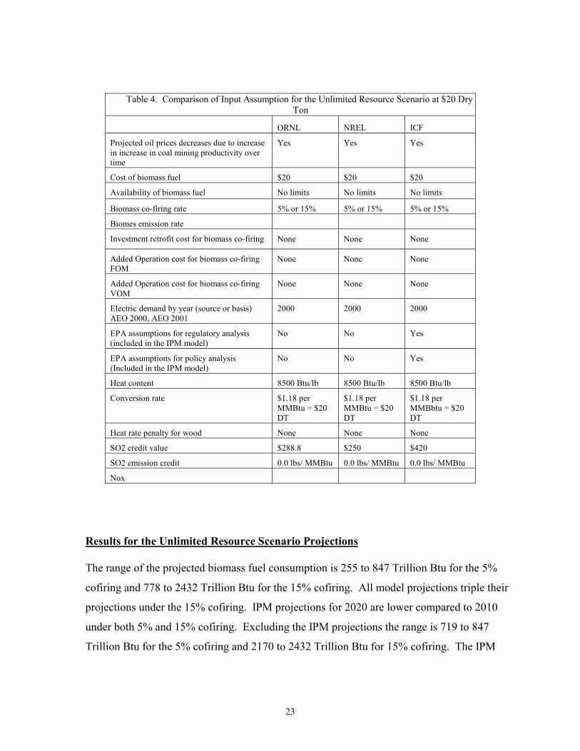
Results for the Unlimited Resource Scenario Projections

The range of the projected biomass fuel consumption is 255 to 847 Trillion Btu for the 5%

cofiring and 778 to 2432 Trillion Btu for the 15% cofiring. All model projections triple their

projections under the 15% cofiring. IPM projections for 2020 are lower compared to 2010

under both 5% and 15% cofiring. Excluding the IPM projections the range is 719 to 847

Trillion Btu for the 5% cofiring and 2170 to 2432 Trillion Btu for 15% cofiring. The IPM

Table 4. Comparison of Input Assumption for the Unlimited Resource Scenario at $20 Dry Ton

ORNL NREL ICF

Projected oil prices decreases due to increase in increase in coal mining productivity over time

Yes Yes Yes

Cost of biomass fuel $20 $20 $20

Availability of biomass fuel No limits No limits No limits

Biomass co-firing rate 5% or 15% 5% or 15% 5% or 15%

Biomes emission rate

Investment retrofit cost for biomass co-firing None None None

Added Operation cost for biomass co-firing FOM

None None None

Added Operation cost for biomass co-firing VOM

None None None

Electric demand by year (source or basis) AEO 2000, AEO 2001

2000 2000 2000

EPA assumptions for regulatory analysis (included in the IPM model)

No No Yes

EPA assumptions for policy analysis (Included in the IPM model)

No No Yes

Heat content 8500 Btu/lb 8500 Btu/lb 8500 Btu/lb

Conversion rate $1.18 per MMBtu = $20 DT

$1.18 per MMBtu = $20 DT

$1.18 per MMBbtu = $20 DT

Heat rate penalty for wood None None None

SO2 credit value $288.8 $250 $420

SO2 emission credit 0.0 lbs/ MMBtu 0.0 lbs/ MMBtu 0.0 lbs/ MMBtu

Nox

24

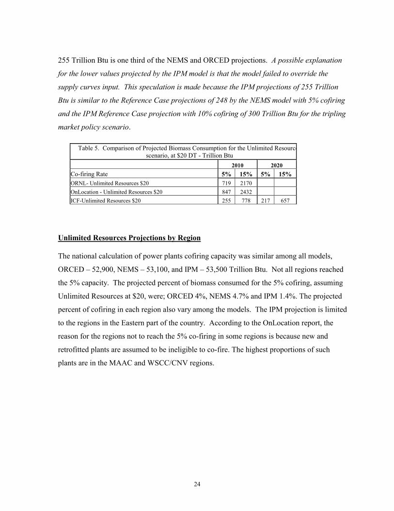
255 Trillion Btu is one third of the NEMS and ORCED projections. A possible explanation

for the lower values projected by the IPM model is that the model failed to override the

supply curves input. This speculation is made because the IPM projections of 255 Trillion

Btu is similar to the Reference Case projections of 248 by the NEMS model with 5% cofiring

and the IPM Reference Case projection with 10% cofiring of 300 Trillion Btu for the tripling

market policy scenario.

Table 5. Comparison of Projected Biomass Consumption for the Unlimited Resourcescenario, at $20 DT - Trillion Btu

2010 2020 Co-firing Rate 5% 15% 5% 15% ORNL- Unlimited Resources $20 719 2170 OnLocation - Unlimited Resources $20 847 2432 ICF-Unlimited Resources $20 255 778 217 657

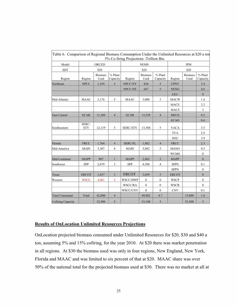
Unlimited Resources Projections by Region

The national calculation of power plants cofiring capacity was similar among all models,

ORCED – 52,900, NEMS – 53,100, and IPM – 53,500 Trillion Btu. Not all regions reached

the 5% capacity. The projected percent of biomass consumed for the 5% cofiring, assuming

Unlimited Resources at $20, were; ORCED 4%, NEMS 4.7% and IPM 1.4%. The projected

percent of cofiring in each region also vary among the models. The IPM projection is limited

to the regions in the Eastern part of the country. According to the OnLocation report, the

reason for the regions not to reach the 5% co-firing in some regions is because new and

retrofitted plants are assumed to be ineligible to co-fire. The highest proportions of such

plants are in the MAAC and WSCC/CNV regions.

25

Results of OnLocation Unlimited Resources Projections

OnLocation projected biomass consumed under Unlimited Resources for $20, $30 and $40 a

ton, assuming 5% and 15% cofiring, for the year 2010. At $20 there was market penetration

in all regions. At $30 the biomass used was only in four regions, New England, New York,

Florida and MAAC and was limited to six percent of that at $20. MAAC share was over

50% of the national total for the projected biomass used at $30. There was no market at all at

Table 6. Comparison of Regional Biomass Consumption Under the Unlimited Resources at $20 a ton5% Co-firing Projections -Trillion Btu

Model ORCED NEMS IPM

$DT $20 $20 $20

Region Region Biomass

Used % Plant Capacity Region

Biomass Used

% Plant Capacity Region

Biomass Used

% Plant Capacity

Northeast NPCC 1,254 5 NPCC/NY 824 5 UPNY 3.4 NPCC/NE 647 5 NENG 4.6 LILC 0

Mid-Atlantic MAAC 3,176 5 MAAC 3,000 3 MACW 1.4 MACE 3.2 MACS 3

East Central ECAR 11,209 4 ECAR 13,529 4 MECS 0.2 ECAO 0.6

Southeastern SERC-STV 12,119 5 SERC-STV 13,588 5 VACA 3.5

TVA 2.9

SOU 3.9

Florida FRCC 1,764 4 SERC/FL 1,882 4 FRCC 2.3

Mid-America MAIN 3,307 4 MAIN 5,882 5 MANO 0.5 WUMS 0

Mid-Continent MAPP 907 1 MAPP 2,882 3 MAPP 0

Southwest SPP 2,679 3 SPP 4,588 4 SPPS 0.1 SPPN 0

Texas ERCOT 1,837 3 ERCOT 3,059 5 ERCOT 0

Western WSCC 4,061 3 WSCC/HWP 0 0 WSCP 0 WSCC/RA 0 0 WSCR 0 WSCC/CNV 0 0 CNV 0.1

Total Consumed Total 42,000 4 49,882 4.7 15,000 1.4

Cofiring Capacity 52,900 5 53,100 5 53,500 5

26

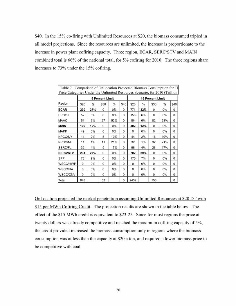
$40. In the 15% co-firing with Unlimited Resources at $20, the biomass consumed tripled in

all model projections. Since the resources are unlimited, the increase is proportionate to the

increase in power plant cofiring capacity. Three region, ECAR, SERC/STV and MAIN

combined total is 66% of the national total, for 5% cofiring for 2010. The three regions share

increases to 73% under the 15% cofiring.

OnLocation projected the market penetration assuming Unlimited Resources at $20 DT with

$15 per MWh Cofiring Credit. The projection results are shown in the table below. The

effect of the $15 MWh credit is equivalent to $23-25. Since for most regions the price at

twenty dollars was already competitive and reached the maximum cofiring capacity of 5%,

the credit provided increased the biomass consumption only in regions where the biomass

consumption was at less than the capacity at $20 a ton, and required a lower biomass price to

be competitive with coal.

Table 7. Comparison of OnLocation Projected Biomass Consumption for ThPrice Categories Under the Unlimited Resources Scenario, for 2010 (Trillion

5 Percent Limit 15 Percent Limit Region $20 % $30 % $40 $20 % $30 % $40

ECAR 230 27% 0 0% 0 771 32% 0 0% 0

ERCOT 52 6% 0 0% 0 156 6% 0 0% 0

MAAC 51 6% 27 52% 0 154 6% 82 53% 0

MAIN 100 12% 0 0% 0 302 12% 0 0% 0

MAPP 49 6% 0 0% 0 0 0% 0 0% 0

NPCC/NY 14 2% 5 10% 0 44 2% 16 10% 0

NPCC/NE 11 1% 11 21% 0 32 1% 32 21% 0

SERC/FL 32 4% 9 17% 0 96 4% 26 17% 0

SERC/STV 231 27% 0 0% 0 702 29% 0 0% 0

SPP 78 9% 0 0% 0 175 7% 0 0% 0

WSCC/HWP 0 0% 0 0% 0 0 0% 0 0% 0

WSCC/RA 0 0% 0 0% 0 0 0% 0 0% 0

WSCC/CNV 0 0% 0 0% 0 0 0% 0 0% 0

Total 848 52 0 2432 156 0

27

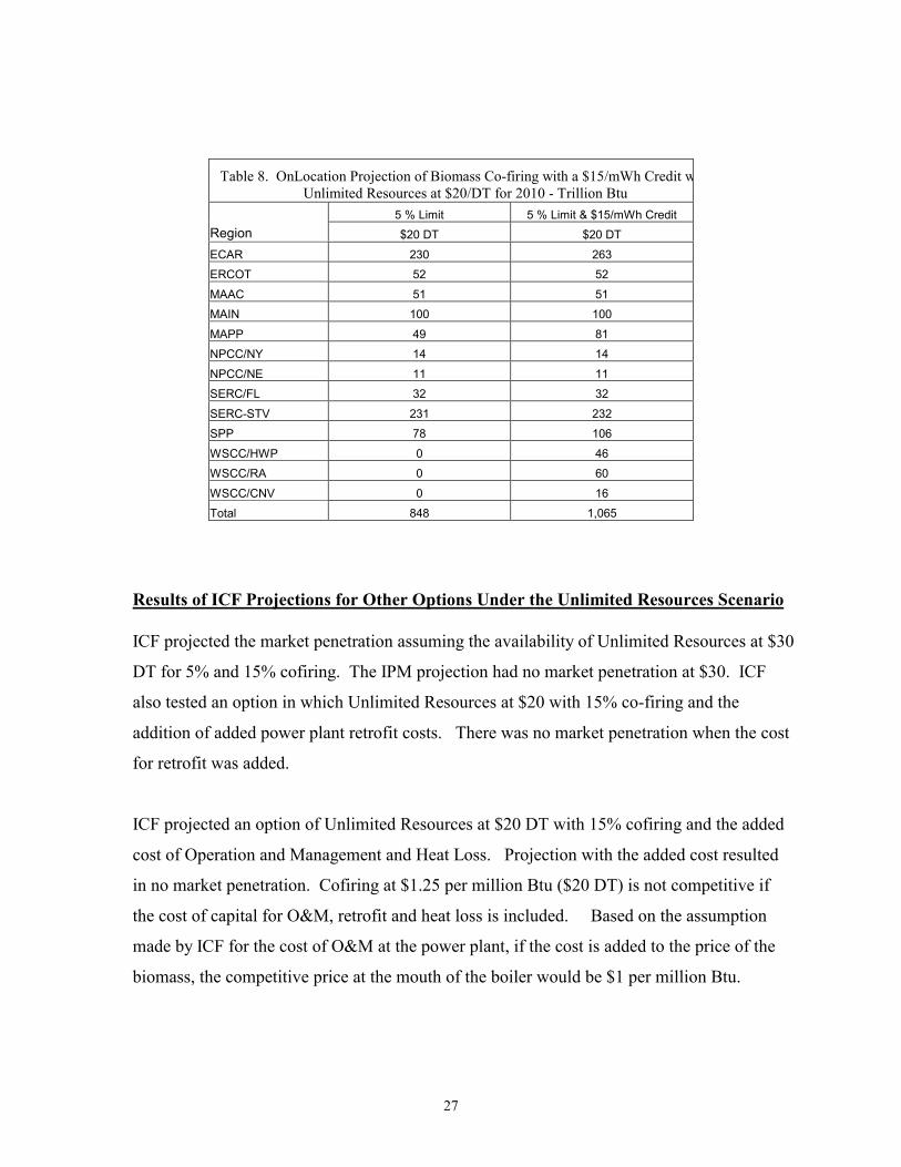
Results of ICF Projections for Other Options Under the Unlimited Resources Scenario

ICF projected the market penetration assuming the availability of Unlimited Resources at $30

DT for 5% and 15% cofiring. The IPM projection had no market penetration at $30. ICF

also tested an option in which Unlimited Resources at $20 with 15% co-firing and the

addition of added power plant retrofit costs. There was no market penetration when the cost

for retrofit was added.

ICF projected an option of Unlimited Resources at $20 DT with 15% cofiring and the added

cost of Operation and Management and Heat Loss. Projection with the added cost resulted

in no market penetration. Cofiring at $1.25 per million Btu ($20 DT) is not competitive if

the cost of capital for O&M, retrofit and heat loss is included. Based on the assumption

made by ICF for the cost of O&M at the power plant, if the cost is added to the price of the

biomass, the competitive price at the mouth of the boiler would be $1 per million Btu.

Table 8. OnLocation Projection of Biomass Co-firing with a $15/mWh Credit wUnlimited Resources at $20/DT for 2010 - Trillion Btu

5 % Limit 5 % Limit & $15/mWh Credit Region $20 DT $20 DT

ECAR 230 263

ERCOT 52 52

MAAC 51 51

MAIN 100 100

MAPP 49 81

NPCC/NY 14 14

NPCC/NE 11 11

SERC/FL 32 32

SERC-STV 231 232

SPP 78 106

WSCC/HWP 0 46

WSCC/RA 0 60

WSCC/CNV 0 16

Total 848 1,065

28

Renewable Portfolio Standards Scenario

EIA projected the potential market for biopower assuming that utilities would be required to

generate electricity with renewable resources. Two options were evaluated one would

require 10% and the other would require 20% of the utility electric generation to be from

renewable resources. The projections assume a 5% co-firing with no added cost for power

plant retrofit. Utilities that do not meet the 10% or 20% requirement would have to pay a

penalty of three cents per kWh. The three cents requirement value is equal to $46-$50. If the

value of the penalty would be applied to the price of biomass, utilities could pay $50-80 per

ton.

The reference Case projected biomass consumption for 2010 as 248 trillion Btu. The 2020

projections of 191 trillion Btu is a decline of 23% compared to 2010 because there are fewer

power plants that could co-fire, and the price of coal is cheaper.

The projections for the 10% RPS for 2010 of 435 trillion Btu are higher by 75% over the

Reference Case and for 2020 of 1182 trillion Btu are four and a half times the reference case

and over three and a half time the 10% RPS for 2010. The biomass consumption for the 20%

RPS for 2010 was 1162 trillion Btu. The highest market penetration of 1492 trillion Btu,

projected for the 20% RPS for the year 2020, is eight times the market penetration of the

reference case for 2020.

The regions with the highest market penetration in both 10% and 20% RPS are ECAR and

SERC/STV. Under the Reference case there are five regions with penetration of over 10% of

the national total, ECAR, SERC/STV, New England, MAAC and WSCC/CNV.

29

Table 9. EIA Projected Biomass Consumption for 10% and 20% RPS for 2010 and 2020Trillion Btu

Reference Case 10% RPS Case 20% RPS Case Region 2010 2020 2010 2020 2010 2020

1 ECAR 40 13 69 299 241 307

2 ERCOT 7 2 25 52 52 52

3 MAAC 27 29 33 60 56 82

4 MAIN 12 5 34 104 137 190

5 MAPP 13 13 13 93 91 130

6 NPCC/NY 15 15 23 27 27 36

7 NPCC/NE 37 38 38 47 47 47

8 FL 18 16 21 41 34 55

9 STV 38 21 77 231 240 306

10 SPP 1 0 51 78 88 88

11 WSCC/NWP 7 7 7 49 31 62

12 WSCC/RA 1 0 6 62 51 62

13 WSCC/CNV 32 32 38 38 67 73

Total US 248 191 435 1182 1162 1492

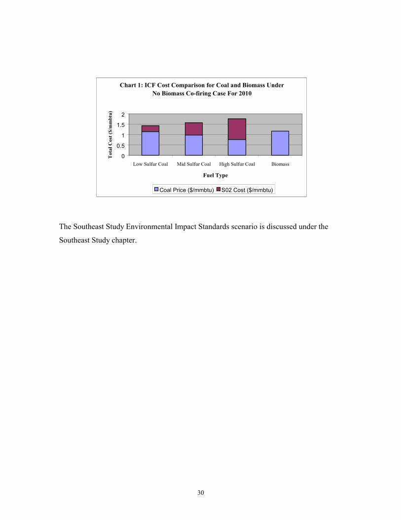
Environmental Impact Standards Scenario

Data for projections made by ICF for Tripling the Market scenario was unavailable. The ICF

memorandums for the Unlimited Resources projections discuss some environmental impact.

The memorandums are included as Appendix 3 and Appendix 4. According to the ICF

calculations, the equivalent price of biomass would vary with the quality of coal. Under the

current SO2 requirements, the equivalent price of biomass in comparison with the different

grade of coal is shown in the chart below. In the case of high sulfur coal, the competitive

price of biomass increases by over 50% to $30 a dry ton. Enabling biomass to be more

competitive in this region with high sulfur.

30

The Southeast Study Environmental Impact Standards scenario is discussed under the

Southeast Study chapter.

Chart 1: ICF Cost Comparison for Coal and Biomass Under No Biomass Co-firing Case For 2010

0

0.5

1

1.5

2

Low Sulfur Coal Mid Sulfur Coal High Sulfur Coal Biomass

Fuel Type

Tot

al C

ost (

$/m

mbt

u)

Coal Price ($/mmbtu) S02 Cost ($/mmbtu)

31

Resources

Two biomass supply databases, one developed by the NEMS and the other developed by

ORNL, were used in the projections. The Biomass Supply Curves provide estimates of

resource availability. Quantities are estimated by resource type, by price category and

measured by either English (short) Dry Ton or by Trillion Btu. ORNL used their biomass

supply estimates in their projections. All the other projections used the NEMS supply

database.

NEMS developed and maintains the biomass supply curves database. The NEMS Supply

Curves were developed from information provided by ORNL, Antares and the U.S.

Department of Agriculture. A recent EIA publication, written by Zia Hag, provides a

thorough explanation of how the data was developed. “The article, Biomass for Electricity

Generation, can be viewed or downloaded from the web at

http://www.eia.doe.gov/oiaf/analysispaper/index.html. The report describes how the

methodology used in NEMS account for various types of biomass and explains the

underlying assumptions. Forecasts of biomass growth under different scenarios are also

presented.

Resource Types

ORNL biomass quantities are estimated by six categories; Urban Wood Waste, Mill

Residues, Forest Residues, Agriculture Residues, Switchgrass, and Short Rotation Wood

Crops. NEMS database includes estimates for four resource types. In the NEMS supply

curves the Mill Residues and the Urban Wood Waste are combined into a single category

named Urban & Mill Residues and the Switchgrass and the Short Rotation Wood Crops are

combined into a category named Energy Crop.

32

Urban Wood Waste is waste from wood yard trimmings, construction residues, and other

waste wood, including discarded consumer wood products pallets, construction waste, and

demolition debris.

a. Mill Residues includes residues from mill operations. Most of the Mill Residues are

used, by industry for industrial by products and internal electric generation and

heating. Only small quantities may be available for utilities electric generation.

c. Forestry residues are the cuttings that remain in forests after logging. Timber

harvesting operations remove only the parts that could be used for lumber. The

remaining branches are left on the ground. Portion of wood that is left on the ground

could be collected and used as fuel for electric generation. Also included in the

estimated forest residues is the collection of rough rotten salvable wood.

d. Agricultural residues are the straw left in the field after harvesting. A portion of the

leftover stalks can be collected and used as energy fuel. Only wheat and corn

residues are included in the estimates. The two represent the majority of all growing

crops that could be usefully collected as biomass.

e. Switchgrass is a species of grasses that are grown for pasture and soil erosion

protection. The grasses that currently are grown are mainly on Conservation Reserve

Program (CRP) land. Farmers have extensive experience with growing switchgrass.

Switchgrass however has not been used in the past as an energy crop. The current

yield can be substantially improved with continuous genetic research that would

make the crop more competitive as an energy source.

f. Short Rotation Wood Crop (SRWC), are plants that are grown for use as energy fuel.

Only two plant species are included in the supply estimates, hybrid poplar and hybrid

willow.

The NEMS biomass resources database will be referred to as NEMS Supply Curve and the

ORNL database as the ORNL Supply Curve. Both supply curves have been compiled and

updated over the past fifteen years. The NEMS Supply Curve provides estimates for the

33

years 1990 and 2000 through 2025. The ORNL Supply Curve provides estimates for the year

2008. Both supply curves assume that the annual estimated supply of residues remain the

same over the years. The increases in availability of biomass over time are due to the

increase in the availability of the Energy Crops. Each price category in both the NEMS and

ORNL supply curves include $10 for transportation from the farm gate to the power plant

gate. They both also assumed that energy crops would not be grown in the three arid regions

of the west.

The NEMS supply curve provide resource availability for 46 price categories ranging from

0.474 MMBtu ($8 DT) to 6.756 MMBtu ($115 DT) in 1987$ or 0.654 to 9.316 MMBtu ($11

to $158 DT) in 2000$. ORNL supply curve estimates are for four price categories, $20, $30,

$40, and $50 DT. NEMS supplies are based on 1987$ and adjusted to 2000$ for the 2020

supplies. The the supply prices for 2020 is adjusted by a factor of 1.38. ORNL supply prices

are based on 1999$ the estimates are for the year 2008. Both supply curves assume that there

will not be a change in the total amount of biomass residues over time. The quantities in

each residue type, Forest residues, Urban Waste and Mill residues and Agriculture residues,

remain the same for the years 2010 through 2020. Each price category includes $10 for

transportation between the farm gate and the power plant gate.

NEMS Supply Curves

The total annual biomass supply estimates are; for the year 2000, 5602 trillion Btu or 330

million dry ton, for the year 2010, 6585 trillion Btu or 387 million dry ton, and for the year

2020, 7102 trillion Btu or 418 million dry ton.

NEMS Supply Estimates by Resource Type

In 2010 thirty five percent of the total resources are estimated to be in Agriculture Residues

and thirty one percent in Forest Residues. Nineteen percent of the total is in Urban Wood

Waste and Mill Residues and fifteen percent are in Energy Crops. The combined forest and

agriculture residues account for sixty six percent of the total.

34

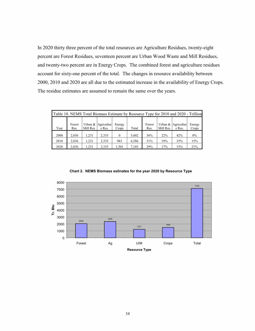
In 2020 thirty three percent of the total resources are Agriculture Residues, twenty-eight

percent are Forest Residues, seventeen percent are Urban Wood Waste and Mill Residues,

and twenty-two percent are in Energy Crops. The combined forest and agriculture residues

account for sixty-one percent of the total. The changes in resource availability between

2000, 2010 and 2020 are all due to the estimated increase in the availability of Energy Crops.

The residue estimates are assumed to remain the same over the years.

Table 10. NEMS Total Biomass Estimate by Resource Type for 2010 and 2020 - Trillion

Year Forest Res.

Urban & Mill Res.

Agriculture Res.

Energy Crops Total

Forest Res.

Urban & Mill Res.

Agriculture Res.

Energy Crops

2000 2,036 1,231 2,335 0 5,602 36% 22% 42% 0%

2010 2,036 1,231 2,335 983 6,586 31% 19% 35% 15%

2020 2,036 1,231 2,335 1,501 7,103 29% 17% 33% 21%

Chart 2. NEMS Biomass estinates for the year 2020 by Resource Type

20422335

12311495

7103

0

1000

2000

3000

4000

5000

6000

7000

8000

Forest Ag U/M Crops Total

Resource Type

Tr. B

tu

35

NEMS Biomass Supply Estimate by Resource Type by Price

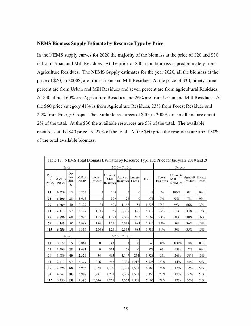
In the NEMS supply curves for 2020 the majority of the biomass at the price of $20 and $30

is from Urban and Mill Residues. At the price of $40 a ton biomass is predominately from

Agriculture Residues. The NEMS Supply estimates for the year 2020, all the biomass at the

price of $20, in 2000$, are from Urban and Mill Residues. At the price of $30, ninety-three

percent are from Urban and Mill Residues and seven percent are from agricultural Residues.

At $40 almost 60% are Agriculture Residues and 26% are from Urban and Mill Residues. At

the $60 price category 41% is from Agriculture Residues, 23% from Forest Residues and

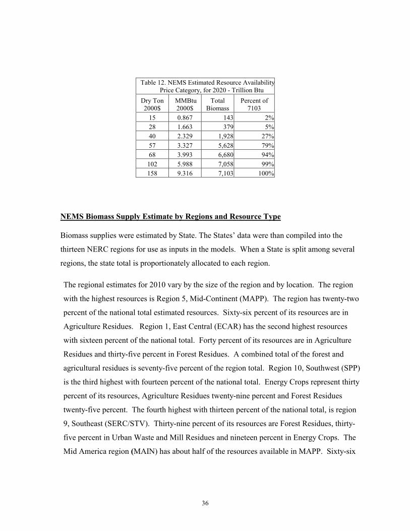
22% from Energy Crops. The available resources at $20, in 2000$ are small and are about

2% of the total. At the $30 the available resources are 5% of the total. The available

resources at the $40 price are 27% of the total. At the $60 price the resources are about 80%

of the total available biomass.

Table 11. NEMS Total Biomass Estimates by Resource Type and Price for the years 2010 and 20

Price 2010 – Tr. Btu Percent

Dry Ton

1987$

MMBtu 1987$

Dry Ton 2000

$

MMBtu 2000$

Forest Residues

Urban & Mill

Residues

Agricult Residues

Energy Crops Total Forest

Residues

Urban & Mill Residues

Agricult Residues

Energy Crops

11 0.629 15 0.867 0 143 0 0 143 0% 100% 0% 0%

21 1.206 28 1.663 0 353 26 0 379 0% 93% 7% 0%

29 1.689 40 2.329 34 493 1,147 54 1,728 2% 29% 66% 3%

41 2.413 57 3.327 1,316 765 2,335 895 5,312 25% 14% 44% 17%

49 2.896 68 3.993 1,724 1,120 2,335 983 6,162 28% 18% 38% 16%

74 4.343 102 5.988 1,991 1,231 2,335 983 6,540 30% 19% 36% 15%

115 6.756 158 9.316 2,036 1,231 2,335 983 6,586 31% 19% 35% 15%

Price 2020 – Tr. Btu

11 0.629 15 0.867 0 143 0 0 143 0% 100% 0% 0%

21 1.206 28 1.663 0 353 26 0 379 0% 93% 7% 0%

29 1.689 40 2.329 34 493 1,147 254 1,928 2% 26% 59% 13%

41 2.413 57 3.327 1,316 765 2,335 1,212 5,628 23% 14% 41% 22%

49 2.896 68 3.993 1,724 1,120 2,335 1,501 6,680 26% 17% 35% 22%

74 4.343 102 5.988 1,991 1,231 2,335 1,501 7,058 28% 17% 33% 21%

115 6.756 158 9.316 2,036 1,231 2,335 1,501 7,103 29% 17% 33% 21%

36

NEMS Biomass Supply Estimate by Regions and Resource Type

Biomass supplies were estimated by State. The States’ data were than compiled into the

thirteen NERC regions for use as inputs in the models. When a State is split among several

regions, the state total is proportionately allocated to each region.

The regional estimates for 2010 vary by the size of the region and by location. The region

with the highest resources is Region 5, Mid-Continent (MAPP). The region has twenty-two

percent of the national total estimated resources. Sixty-six percent of its resources are in

Agriculture Residues. Region 1, East Central (ECAR) has the second highest resources

with sixteen percent of the national total. Forty percent of its resources are in Agriculture

Residues and thirty-five percent in Forest Residues. A combined total of the forest and

agricultural residues is seventy-five percent of the region total. Region 10, Southwest (SPP)

is the third highest with fourteen percent of the national total. Energy Crops represent thirty

percent of its resources, Agriculture Residues twenty-nine percent and Forest Residues

twenty-five percent. The fourth highest with thirteen percent of the national total, is region

9, Southeast (SERC/STV). Thirty-nine percent of its resources are Forest Residues, thirty-

five percent in Urban Waste and Mill Residues and nineteen percent in Energy Crops. The

Mid America region (MAIN) has about half of the resources available in MAPP. Sixty-six

Table 12. NEMS Estimated Resource AvailabilityPrice Category, for 2020 - Trillion Btu

Dry Ton 2000$

MMBtu 2000$

Total Biomass

Percent of 7103

15 0.867 143 2%28 1.663 379 5%40 2.329 1,928 27%57 3.327 5,628 79%68 3.993 6,680 94%

102 5.988 7,058 99%158 9.316 7,103 100%

37

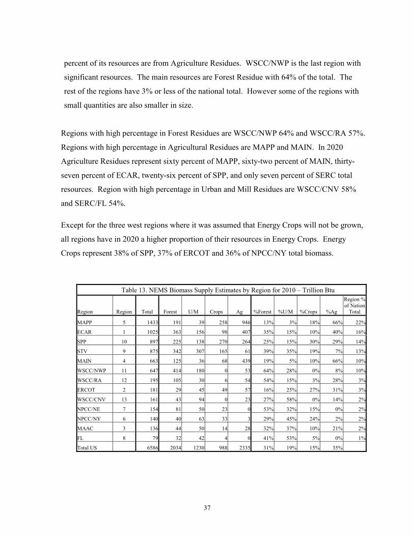
percent of its resources are from Agriculture Residues. WSCC/NWP is the last region with

significant resources. The main resources are Forest Residue with 64% of the total. The

rest of the regions have 3% or less of the national total. However some of the regions with

small quantities are also smaller in size.

Regions with high percentage in Forest Residues are WSCC/NWP 64% and WSCC/RA 57%.

Regions with high percentage in Agricultural Residues are MAPP and MAIN. In 2020

Agriculture Residues represent sixty percent of MAPP, sixty-two percent of MAIN, thirty-

seven percent of ECAR, twenty-six percent of SPP, and only seven percent of SERC total

resources. Region with high percentage in Urban and Mill Residues are WSCC/CNV 58%

and SERC/FL 54%.

Except for the three west regions where it was assumed that Energy Crops will not be grown,

all regions have in 2020 a higher proportion of their resources in Energy Crops. Energy

Crops represent 38% of SPP, 37% of ERCOT and 36% of NPCC/NY total biomass.

Table 13. NEMS Biomass Supply Estimates by Region for 2010 – Trillion Btu

Region Region Total Forest U/M Crops Ag %Forest %U/M %Crops %Ag

Region % of Nation

Total

MAPP 5 1433 191 39 258 946 13% 3% 18% 66% 22%

ECAR 1 1025 363 156 98 407 35% 15% 10% 40% 16%

SPP 10 897 225 138 270 264 25% 15% 30% 29% 14%

STV 9 875 342 307 165 61 39% 35% 19% 7% 13%

MAIN 4 663 125 36 68 439 19% 5% 10% 66% 10%

WSCC/NWP 11 647 414 180 0 53 64% 28% 0% 8% 10%

WSCC/RA 12 195 105 30 6 54 54% 15% 3% 28% 3%

ERCOT 2 181 29 45 49 57 16% 25% 27% 31% 3%

WSCC/CNV 13 161 43 94 0 23 27% 58% 0% 14% 2%

NPCC/NE 7 154 81 50 23 0 53% 32% 15% 0% 2%

NPCC/NY 6 140 40 63 33 3 29% 45% 24% 2% 2%

MAAC 3 136 44 50 14 28 32% 37% 10% 21% 2%

FL 8 79 32 42 4 0 41% 53% 5% 0% 1%

Total US 6586 2034 1230 988 2335 31% 19% 15% 35%

38

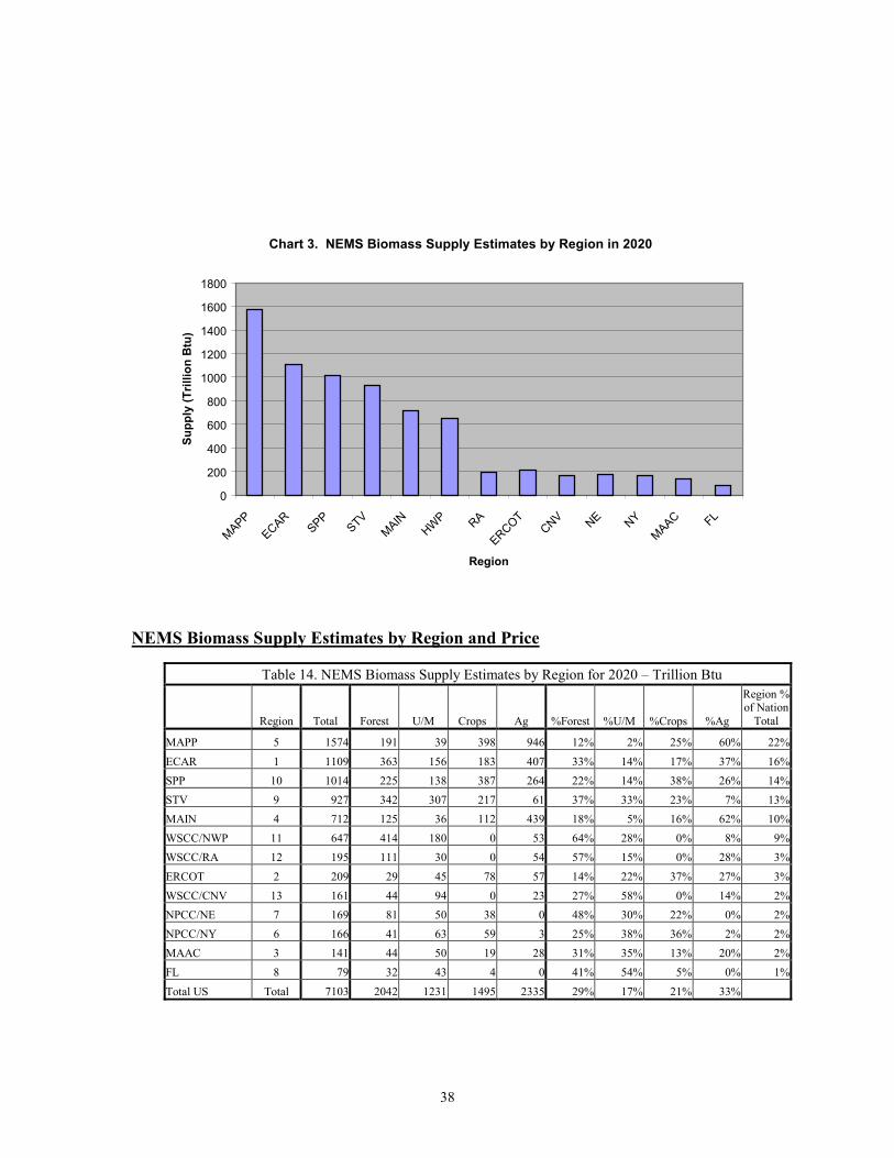
Chart 3. NEMS Biomass Supply Estimates by Region in 2020

0

200

400

600

800

1000

1200

1400

1600

1800

MAPPECAR

SPPSTV

MAINHW

P RA

ERCOTCNV NE NY

MAAC FL

Region

Supp

ly (T

rillio

n B

tu)

NEMS Biomass Supply Estimates by Region and Price

Table 14. NEMS Biomass Supply Estimates by Region for 2020 – Trillion Btu

Region Total Forest U/M Crops Ag %Forest %U/M %Crops %Ag

Region % of Nation

Total

MAPP 5 1574 191 39 398 946 12% 2% 25% 60% 22%

ECAR 1 1109 363 156 183 407 33% 14% 17% 37% 16%SPP 10 1014 225 138 387 264 22% 14% 38% 26% 14%STV 9 927 342 307 217 61 37% 33% 23% 7% 13%MAIN 4 712 125 36 112 439 18% 5% 16% 62% 10%WSCC/NWP 11 647 414 180 0 53 64% 28% 0% 8% 9%WSCC/RA 12 195 111 30 0 54 57% 15% 0% 28% 3%

ERCOT 2 209 29 45 78 57 14% 22% 37% 27% 3%WSCC/CNV 13 161 44 94 0 23 27% 58% 0% 14% 2%NPCC/NE 7 169 81 50 38 0 48% 30% 22% 0% 2%NPCC/NY 6 166 41 63 59 3 25% 38% 36% 2% 2%MAAC 3 141 44 50 19 28 31% 35% 13% 20% 2%FL 8 79 32 43 4 0 41% 54% 5% 0% 1%

Total US Total 7103 2042 1231 1495 2335 29% 17% 21% 33%

39

The percentage, in each price category, for each region, for the year 2020 is shown in the

table below. In most regions the pattern is similar to the national pattern.

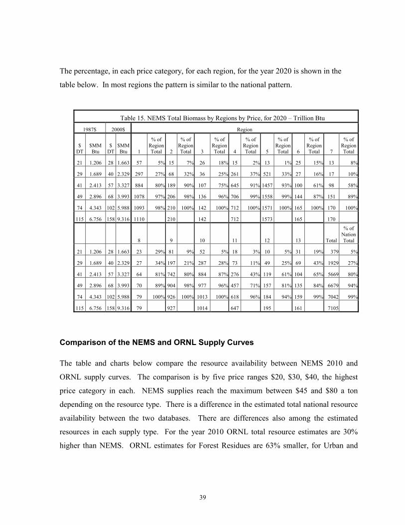
Comparison of the NEMS and ORNL Supply Curves

The table and charts below compare the resource availability between NEMS 2010 and

ORNL supply curves. The comparison is by five price ranges $20, $30, $40, the highest

price category in each. NEMS supplies reach the maximum between $45 and $80 a ton

depending on the resource type. There is a difference in the estimated total national resource

availability between the two databases. There are differences also among the estimated

resources in each supply type. For the year 2010 ORNL total resource estimates are 30%

higher than NEMS. ORNL estimates for Forest Residues are 63% smaller, for Urban and

Table 15. NEMS Total Biomass by Regions by Price, for 2020 – Trillion Btu

1987$ 2000$ Region

$ DT

$MM Btu

$ DT

$MM Btu 1

% of Region Total 2

% of Region Total 3

% of Region Total 4

% of Region Total 5

% of Region Total 6

% of Region Total 7

% of Region Total

21 1.206 28 1.663 57 5% 15 7% 26 18% 15 2% 13 1% 25 15% 13 8%

29 1.689 40 2.329 297 27% 68 32% 36 25% 261 37% 521 33% 27 16% 17 10%

41 2.413 57 3.327 884 80% 189 90% 107 75% 645 91% 1457 93% 100 61% 98 58%

49 2.896 68 3.993 1078 97% 206 98% 136 96% 706 99% 1558 99% 144 87% 151 89%

74 4.343 102 5.988 1093 98% 210 100% 142 100% 712 100% 1571 100% 165 100% 170 100%

115 6.756 158 9.316 1110 210 142 712 1573 165 170

8 9 10 11 12 13 Total

% of Nation Total

21 1.206 28 1.663 23 29% 81 9% 52 5% 18 3% 10 5% 31 19% 379 5%

29 1.689 40 2.329 27 34% 197 21% 287 28% 73 11% 49 25% 69 43% 1929 27%

41 2.413 57 3.327 64 81% 742 80% 884 87% 276 43% 119 61% 104 65% 5669 80%

49 2.896 68 3.993 70 89% 904 98% 977 96% 457 71% 157 81% 135 84% 6679 94%

74 4.343 102 5.988 79 100% 926 100% 1013 100% 618 96% 184 94% 159 99% 7042 99%

115 6.756 158 9.316 79 927 1014 647 195 161 7105

40

Mill Residues 43% higher, for Agriculture residues about 10% higher and for Energy Crops

about three times higher than the NEMS estimates. Significant differences are also exists in

the estimates by price categories. The most notable is ORNL estimate for Agriculture

Residues that is 95% smaller than NEMS.

Chart 4. Comparison of Total Biomass Supply Estimates between NEMS 2010, NEMS 2020 and ORNL

0

1000

2000

3000

4000

5000

6000

7000

8000

9000

10000

For U/M Ag EC Total

Supply Type

Supp

ly T

rBtu

NEMS 2010 NEMS 2020 ORNL

Table 16. Comparison of Biomass Supply Between NEMS and ORNL 2010 Estimates – Trillion Btu

Price per Dry Ton Supply Curve Ag For U/M EC Total

20 NEMS 26 0 353 0 379

20 ORNL 0 0 405 0 404

30 NEMS 1147 34 493 54 1944

30 ORNL 54 40 1331 0 1425

40 NEMS 2335 1316 765 895 5312

40 ORNL 2301 591 1331 1124 5347

Maximum NEMS 2010 2335 2036 1231 983 6586

Maximum NEMS 2020 2335 2036 1231 1,501 7103

Maximum ORNL 2561 763 2163 3197 8684

41

Chart 5. Comparison of Biomass Supply Between NEMS and ORNL $20 DT for 2010

050

100150200250300350400450

For U/M Ag EC Total

Supply Type

RSu

pply

TrB

tu

NEMS ORNL

Chart 6. Comparison of Biomass Supply Curves Between NEMS and ORNL at $30 DT for 2010

0

500

1000

1500

2000

2500

For U/M Ag EC Total

Supply Type

Supp

ly T

rBtu

NEMS ORNL

42

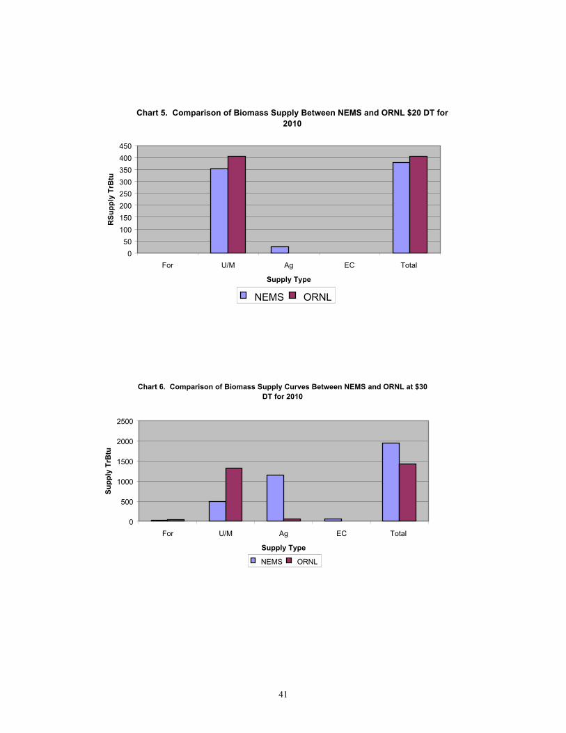
Chart 7. Comparison of Biomass Supply Between NEMS and ORNL at $40 DT for 2010

0100020003000400050006000

For U/M Ag EC Total

Supply Type

Supp

ly T

rBtu

NEMS ORNL

At $40 the supply quantities are about the same in the two databases.

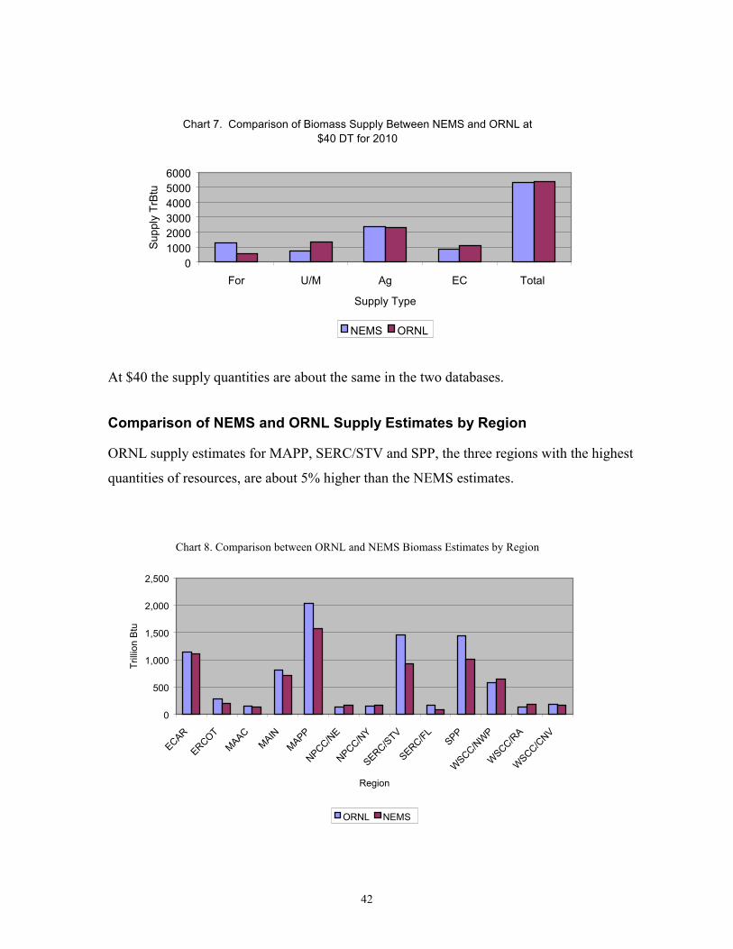
Comparison of NEMS and ORNL Supply Estimates by Region

ORNL supply estimates for MAPP, SERC/STV and SPP, the three regions with the highest

quantities of resources, are about 5% higher than the NEMS estimates.

Chart 8. Comparison between ORNL and NEMS Biomass Estimates by Region

0

500

1,000

1,500

2,000

2,500

ECAR

ERCOTMAAC

MAINMAPP

NPCC/NE

NPCC/NY

SERC/STV

SERC/FLSPP

WSCC/N

WP

WSCC/R

A

WSCC/C

NV

Region

Trill

ion

Btu

ORNL NEMS

43

ICF NEMS Supply Curves

Two sets of the NEMS supply curves provided by ICF were evaluated. The first set has

smaller overall supplies compared with the NEMS data. The second set had several values

that seem to be erroneous. The total estimated resources were about 40% higher than the

EIA-NEMS for 2010. The Forest Residue availability starts at $50 while the EIA-NEMS and

ORNL starts at $30. The Energy Crops has resources at $20 a dry ton while IEA-NEMS and

ORNL start at $40. The second set seems to be completely out of character with the IEA

NEMS data.

The analysis reveals that different version of the NEMS and ORNL supply curves were used

by different agencies and by the same agency for different projections.

44

Analysis - Comparison of Resource Availability with Projected Market Demand

The objective of the evaluation is to determine the correlation between biomass availability

and the biomass demand based on the level of market penetration under each scenario. The

comparison between the scenarios is difficult. Each projection was made with different input

assumptions, different subsidy level and different assumption of resource availability.

Except for the RPS all projections were limited to cofiring. The RPS projections included

cofiring, dedicated plants and industrial cogeneration. The market level achieved under each

option was determined by the biomass price and the availability of the resource at the

competitive price reached by the option. Projections of biomass consumption were made for

several options for four scenarios. The results of the projections provide a general picture of

the range of market potential that might be feasible if one or more of the policy scenario

would be mandated. Conclusion were drawn based on the analysis that included; comparison

of the projected resources used and resource availability; whether there were adequate

resources to meet the demand at the projected biomass purchased price; at what biomass

prices resource availability limited penetration; what was the main resource type used; and

were there any constraints that might limit the availability of resources at the purchased price

category. The results of the analysis provided an understanding of the level of incentive that

would be needed and the implication on resource policies and research to achieve an increase

in the biopower market.

Comparison of resource used and total resource availability

The table below compares the total biomass estimated by NEMS with the projected biomass

consumed under each of the major options for each scenario.

There are adequate resources to meet the projected resource demand for all the projections.

The Unlimited Resources assume that the total estimated resources were available at $20 a

dry ton. Under the projection of Unlimited Resources 33-37% of the available resources

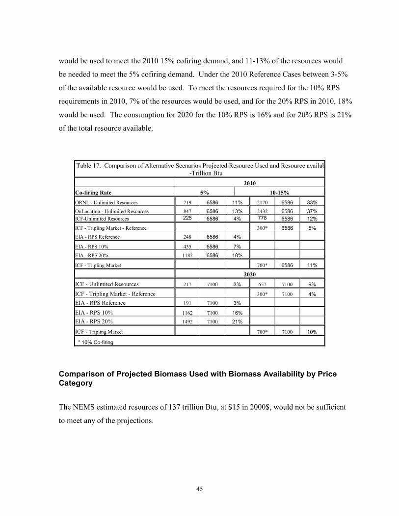
45

would be used to meet the 2010 15% cofiring demand, and 11-13% of the resources would

be needed to meet the 5% cofiring demand. Under the 2010 Reference Cases between 3-5%

of the available resource would be used. To meet the resources required for the 10% RPS

requirements in 2010, 7% of the resources would be used, and for the 20% RPS in 2010, 18%

would be used. The consumption for 2020 for the 10% RPS is 16% and for 20% RPS is 21%

of the total resource available.

Comparison of Projected Biomass Used with Biomass Availability by Price Category

The NEMS estimated resources of 137 trillion Btu, at $15 in 2000$, would not be sufficient

to meet any of the projections.

Table 17. Comparison of Alternative Scenarios Projected Resource Used and Resource availab-Trillion Btu

2010 Co-firing Rate 5% 10-15%

ORNL - Unlimited Resources 719 6586 11% 2170 6586 33% OnLocation - Unlimited Resources 847 6586 13% 2432 6586 37% ICF-Unlimited Resources 225 6586 4% 778 6586 12%

ICF - Tripling Market - Reference 300* 6586 5% EIA - RPS Reference 248 6586 4%

EIA - RPS 10% 435 6586 7% EIA - RPS 20% 1182 6586 18%

ICF - Tripling Market 700* 6586 11%

2020 ICF - Unlimited Resources 217 7100 3% 657 7100 9%

ICF - Tripling Market - Reference 300* 7100 4% EIA - RPS Reference 191 7100 3%

EIA - RPS 10% 1162 7100 16% EIA - RPS 20% 1492 7100 21%

ICF - Tripling Market 700* 7100 10%

* 10% Co-firing

46

The NEMS estimated biomass of 379 trillion Btu, at $20 based on 1987$, or at $30 based on

2000$, would be enough to meet the demand of the Reference Cases projection. Over 60%

of the estimated resources would be used. There aren’t enough resources to meet the demand

of any of the other projections.

The NEMS estimated biomass of 1944 trillion Btu, at $30 based on 1987$, or at $40 based

on 2000$, would be enough to satisfied the projected need of the RPS projections in 2010

and 2020, under both the 10% and the 20% RPS. Twenty-two percent of the NEMS

estimated available resource would be used to meet the demand of the 2010 10% RPS. The

percentage is 60% for the 2010 20% RPS and the 2020 10% RPS. 77% of the estimated

available resources would be needed to meet the 2020 20% RPS.

The NEMS estimated available resources of 5312 trillion Btu, at $40 based on 1987$, or at

$60 based on 2000$, are enough to meet the projected demand of all scenarios.

Comparison of Supply and Projected Demand for the Unlimited Resources Scenario

The Unlimited Resources projections represent the maximum potential for cofiring under

either the 5% or the 15% cofiring and the projected year. There are not enough resources to

meet the projected potential at the competitive price of $20 a dry ton. Adequate resources

are available at $30, 1987$ or at $40, 2000$ for 5% cofiring in 2010 in which 40% of the

resources are used. There are not enough resources at this price to meet the demand for 15%

cofiring. There are adequate resources to meet the demand under the $40, 1987$ or $60,

2000$ price category for both 5% and 15% cofiring. The projected demand is 15% of the

available biomass for the 5% cofiring and 43% for the 15% cofiring for 2010.

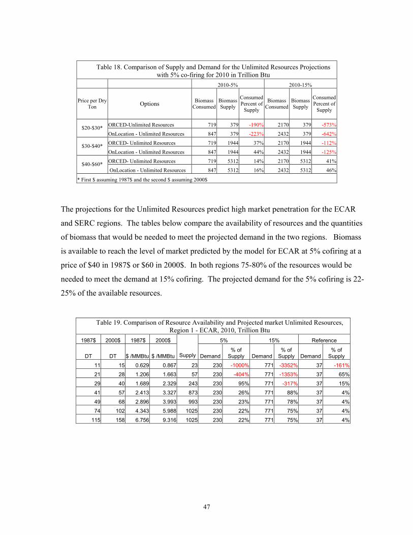
47

The projections for the Unlimited Resources predict high market penetration for the ECAR

and SERC regions. The tables below compare the availability of resources and the quantities

of biomass that would be needed to meet the projected demand in the two regions. Biomass

is available to reach the level of market predicted by the model for ECAR at 5% cofiring at a

price of $40 in 1987$ or $60 in 2000$. In both regions 75-80% of the resources would be

needed to meet the demand at 15% cofiring. The projected demand for the 5% cofiring is 22-

25% of the available resources.

Table 19. Comparison of Resource Availability and Projected market Unlimited Resources, Region 1 - ECAR, 2010, Trillion Btu

1987$ 2000$ 1987$ 2000$ 5% 15% Reference

DT DT $ /MMBtu $ /MMBtu Supply Demand% of

Supply Demand% of

Supply Demand % of

Supply

11 15 0.629 0.867 23 230 -1000% 771 -3352% 37 -161%

21 28 1.206 1.663 57 230 -404% 771 -1353% 37 65%

29 40 1.689 2.329 243 230 95% 771 -317% 37 15%

41 57 2.413 3.327 873 230 26% 771 88% 37 4%

49 68 2.896 3.993 993 230 23% 771 78% 37 4%

74 102 4.343 5.988 1025 230 22% 771 75% 37 4%

115 158 6.756 9.316 1025 230 22% 771 75% 37 4%

Table 18. Comparison of Supply and Demand for the Unlimited Resources Projections with 5% co-firing for 2010 in Trillion Btu

2010-5% 2010-15%

Price per Dry Ton Options Biomass

ConsumedBiomass Supply

Consumed Percent of

Supply

Biomass Consumed

Biomass Supply

Consumed Percent of

Supply

ORCED-Unlimited Resources 719 379 -190% 2170 379 -573%$20-$30* OnLocation - Unlimited Resources 847 379 -223% 2432 379 -642%

ORCED- Unlimited Resources 719 1944 37% 2170 1944 -112%$30-$40* OnLocation - Unlimited Resources 847 1944 44% 2432 1944 -125%

ORCED- Unlimited Resources 719 5312 14% 2170 5312 41%$40-$60* OnLocation - Unlimited Resources 847 5312 16% 2432 5312 46%

* First $ assuming 1987$ and the second $ assuming 2000$

48

Renewable Portfolio Standards

RPS Comparison by Price

As shown in the table below, there are enough resources at the $30 in 1987$ or $40 in 2000$

to meet the projected demand for all options. However, in the year 2020, 60% of the

resource be used for the 10% RPS and 77% would use and the 20% RPS.

Table 20. Comparison of Resource Availability and Projected market Unlimited Resources, Region 9 SERC, 2010, Trillion Btu

1987$ 2000$ 1987$ 2000$ 5% 15% Reference

DT DT $ /MMBtu $ /MMBtu Supply Demand % of

Supply Demand % of

Supply Demand % of Supply

11 15 0.629 0.867 22 231 -1050% 702 -3191% 47 -214%

21 28 1.206 1.663 81 231 -285% 702 -867% 47 58%

29 40 1.689 2.329 156 231 -148% 702 -450% 47 30%

41 57 2.413 3.327 691 231 33% 702 -102% 47 7%

49 68 2.896 3.993 852 231 27% 702 82% 47 6%

74 102 4.343 5.988 875 231 26% 702 80% 47 5%

115 158 6.756 9.316 875 231 26% 702 80% 47 5%

Table 21. Comparison of Projected RPS Demand with Biomass Supply by Price– Trillion Btu Price per Ton 2010 2020

1987$ 2000$ 1987$ 2000$ 2010 2010-10% 2010-20% 2020 2020-10% 2020-20%

$D/Ton $D/Ton MMBtu MMBtu Supply Used % Used % Supply Used % Used %

11 15 0.629 0.867 143 435 -304% 1162 -813% 143 1182 -827% 1492 -1043%

21 28 1.206 1.663 379 435 -115% 1162 -307% 379 1182 -312% 1492 -394%

29 40 1.689 2.329 1944 435 22% 1162 60% 1928 1182 61% 1492 77%

41 57 2.413 3.327 5312 435 8% 1162 22% 5628 1182 21% 1492 27%

49 68 2.896 3.993 6162 435 7% 1162 19% 6680 1182 18% 1492 22%

74 102 4.343 5.988 6540 435 7% 1162 18% 7058 1182 17% 1492 21%

115 158 6.756 9.316 6586 435 7% 1162 18% 7103 1182 17% 1492 21%

49

RPS Comparison by Region

The table below compares the biomass supply with the projected biomass consumed in each

region. The first six regions with the highest biomass supply consumed between 1% and 9%

and the six regions with the lowest biomass supplies consumed between 14% and 27% under

the 10% RPS for 2010. The first six regions with the highest biomass supply consumed

between 6% and 25% and the six regions with the lowest biomass supplies consumed

between 17% and 53% of the regions available resources under the 10% RPS for 2020.

The two regions with the highest market share ECAR consumed 7% in 2010 and 27% in

2020 and SERC/STV consumed 9% in 2010 and 25 % in 2020 of the estimated biomass

supply.

The comparison of the availability of resources with the projected use for ECAR and SERC

are shown in the tables below. At the price category of $30 in 1987$ or $40 in 2000$, there

would be enough biomass in ECAR to meet the projected demand under the 10% RPS for

2010 and 2020. However, 81% of the resources would be used in 2020. There are not

Table 22. Biomass Consumption by Region for RPS 10% - Trillion Btu 2010 2020 Used Avail % Used Avail % MAPP 13 1433 1% 93 1574 6%ECAR 69 1025 7% 299 1109 27%SPP 51 897 6% 78 1014 8%STV 77 875 9% 231 927 25%MAIN 34 663 5% 104 712 15%WSCC/NWP 7 647 1% 49 647 8%WSCC/RA 6 195 3% 62 189 33%ERCOT 25 181 14% 52 209 25%WSCC/CNV 38 161 23% 38 160 24%NPCC/NE 38 154 25% 47 169 28%NPCC/NY 23 140 17% 27 165 17%MAAC 33 136 24% 60 141 43%FL 21 79 27% 41 78 53%Total US 435 6586 7% 1182 7094 17%

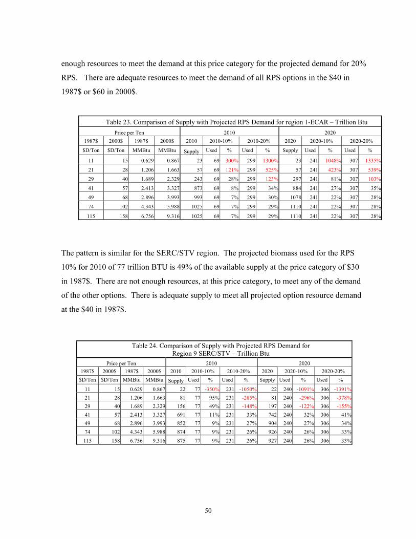
50

enough resources to meet the demand at this price category for the projected demand for 20%

RPS. There are adequate resources to meet the demand of all RPS options in the $40 in

1987$ or $60 in 2000$.

The pattern is similar for the SERC/STV region. The projected biomass used for the RPS

10% for 2010 of 77 trillion BTU is 49% of the available supply at the price category of $30

in 1987$. There are not enough resources, at this price category, to meet any of the demand

of the other options. There is adequate supply to meet all projected option resource demand

at the $40 in 1987$.

Table 24. Comparison of Supply with Projected RPS Demand for Region 9 SERC/STV – Trillion Btu

Price per Ton 2010 2020 1987$ 2000$ 1987$ 2000$ 2010 2010-10% 2010-20% 2020 2020-10% 2020-20%

$D/Ton $D/Ton MMBtu MMBtu Supply Used % Used % Supply Used % Used %

11 15 0.629 0.867 22 77 -350% 231 -1050% 22 240 -1091% 306 -1391%21 28 1.206 1.663 81 77 95% 231 -285% 81 240 -296% 306 -378%29 40 1.689 2.329 156 77 49% 231 -148% 197 240 -122% 306 -155%41 57 2.413 3.327 691 77 11% 231 33% 742 240 32% 306 41%49 68 2.896 3.993 852 77 9% 231 27% 904 240 27% 306 34%74 102 4.343 5.988 874 77 9% 231 26% 926 240 26% 306 33%

115 158 6.756 9.316 875 77 9% 231 26% 927 240 26% 306 33%

Table 23. Comparison of Supply with Projected RPS Demand for region 1-ECAR – Trillion Btu Price per Ton 2010 2020

1987$ 2000$ 1987$ 2000$ 2010 2010-10% 2010-20% 2020 2020-10% 2020-20%

$D/Ton $D/Ton MMBtu MMBtu Supply Used % Used % Supply Used % Used %

11 15 0.629 0.867 23 69 300% 299 1300% 23 241 1048% 307 1335%

21 28 1.206 1.663 57 69 121% 299 525% 57 241 423% 307 539%

29 40 1.689 2.329 243 69 28% 299 123% 297 241 81% 307 103%

41 57 2.413 3.327 873 69 8% 299 34% 884 241 27% 307 35%

49 68 2.896 3.993 993 69 7% 299 30% 1078 241 22% 307 28%

74 102 4.343 5.988 1025 69 7% 299 29% 1110 241 22% 307 28%

115 158 6.756 9.316 1025 69 7% 299 29% 1110 241 22% 307 28%

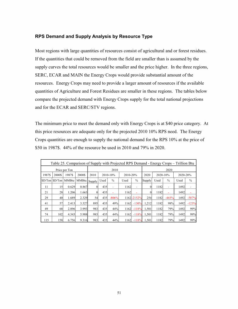
51

RPS Demand and Supply Analysis by Resource Type

Most regions with large quantities of resources consist of agricultural and or forest residues.

If the quantities that could be removed from the field are smaller than is assumed by the

supply curves the total resources would be smaller and the price higher. In the three regions,

SERC, ECAR and MAIN the Energy Crops would provide substantial amount of the

resources. Energy Crops may need to provide a larger amount of resources if the available

quantities of Agriculture and Forest Residues are smaller in these regions. The tables below

compare the projected demand with Energy Crops supply for the total national projections

and for the ECAR and SERC/STV regions.

The minimum price to meet the demand only with Energy Crops is at $40 price category. At

this price resources are adequate only for the projected 2010 10% RPS need. The Energy

Crops quantities are enough to supply the national demand for the RPS 10% at the price of

$50 in 1987$. 44% of the resource be used in 2010 and 79% in 2020.

Table 25. Comparison of Supply with Projected RPS Demand - Energy Crops – Trillion Btu

Price per Ton 2010 2020 1987$ 2000$ 1987$ 2000$ 2010 2010-10% 2010-20% 2020 2020-10% 2020-20%

$D/Ton $D/Ton MMBtu MMBtu Supply Used % Used % Supply Used % Used %

11 15 0.629 0.867 0 435 - 1162 - 0 1182 - 1492 -

21 28 1.206 1.663 0 435 - 1162 - 0 1182 - 1492 -

29 40 1.689 2.329 54 435 -806% 1162 -2152% 254 1182 -465% 1492 -587%

41 57 2.413 3.327 895 435 49% 1162 -130% 1,212 1182 98% 1492 -123%

49 68 2.896 3.993 983 435 44% 1162 -118% 1,501 1182 79% 1492 99%

74 102 4.343 5.988 983 435 44% 1162 -118% 1,501 1182 79% 1492 99%

115 158 6.756 9.316 983 435 44% 1162 -118% 1,501 1182 79% 1492 99%

52

In the ECAR region Energy Crops supply would be adequate to meet the projected demand

for RPS 10% for 2010 where 70% of the resources be used. There is inadequate Energy

Crops supply to meet any of the other projections.

Table 26. Comparison of Supply with Projected RPS Demand for region 1 ECAR - Energy Crops – TrilBtu

Price per Ton 2010 2020 1987$ 2000$ 1987$ 2000$ 2010 2010-10% 2010-20% 2020 2020-10% 2020-20%

$D/Ton $D/Ton MMBtu MMBtu Supply Used % Used % Supply Used % Used %

11 15 0.629 0.867 0 69 - 299 - 0 241 - 307 -

21 28 1.206 1.663 0 69 - 299 - 0 241 - 307 -

29 40 1.689 2.329 0 69 - 299 - 54 241 -447% 307 -569%

41 57 2.413 3.327 94 69 73% 299 -317% 106 241 -228% 307 -290%

49 68 2.896 3.993 98 69 70% 299 -304% 183 241 -131% 307 -167%

74 102 4.343 5.988 98 69 70% 299 -304% 183 241 -131% 307 -167%

115 158 6.756 9.316 98 69 70% 299 -304% 183 241 -131% 307 -167%

The pattern is the same in the SERC/STV region except that the 44% of the Energy Crop

supply would be used for the projected demand for the RPS 10% in 2010.

Table 27. Comparison of Supply with Projected RPS Demand for region 9 SERC - Energy Crops – Trillion Btu

Price per Ton 2010 2020 1987$ 2000$ 1987$ 2000$ 2010 2010-10% 2010-20% 2020 2020-10% 2020-20%

$D/Ton $D/Ton MMBtu MMBtu Supply Used % Used % Supply Used % Used %

11 15 0.629 0.867 0 77 - 231 - 0 240 - 306 -

21 28 1.206 1.663 0 77 - 231 - 0 240 - 306 -

29 40 1.689 2.329 25 77 -308% 231 -924% 66 240 -364% 306 -464%

41 57 2.413 3.327 132 77 58% 231 -175% 184 240 -130% 306 -166%

49 68 2.896 3.993 165 77 47% 231 -140% 217 240 -111% 306 -141%

74 102 4.343 5.988 165 77 47% 231 -140% 217 240 -111% 306 -141%

115 158 6.756 9.316 165 77 47% 231 -140% 217 240 -111% 306 -141%

To meet the demand for 2020, assuming the NEMS supply curves, half of the resources

would need to come from residues.

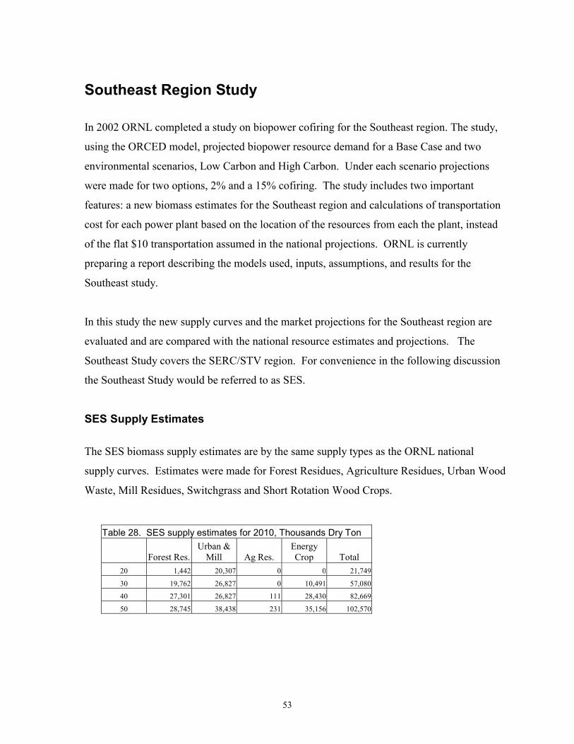
53

Southeast Region Study

In 2002 ORNL completed a study on biopower cofiring for the Southeast region. The study,

using the ORCED model, projected biopower resource demand for a Base Case and two

environmental scenarios, Low Carbon and High Carbon. Under each scenario projections

were made for two options, 2% and a 15% cofiring. The study includes two important

features: a new biomass estimates for the Southeast region and calculations of transportation

cost for each power plant based on the location of the resources from each the plant, instead

of the flat $10 transportation assumed in the national projections. ORNL is currently

preparing a report describing the models used, inputs, assumptions, and results for the

Southeast study.

In this study the new supply curves and the market projections for the Southeast region are

evaluated and are compared with the national resource estimates and projections. The

Southeast Study covers the SERC/STV region. For convenience in the following discussion

the Southeast Study would be referred to as SES.

SES Supply Estimates

The SES biomass supply estimates are by the same supply types as the ORNL national

supply curves. Estimates were made for Forest Residues, Agriculture Residues, Urban Wood

Waste, Mill Residues, Switchgrass and Short Rotation Wood Crops.

Table 28. SES supply estimates for 2010, Thousands Dry Ton

Forest Res. Urban &

Mill Ag Res. Energy Crop Total

20 1,442 20,307 0 0 21,749

30 19,762 26,827 0 10,491 57,080

40 27,301 26,827 111 28,430 82,669

50 28,745 38,438 231 35,156 102,570

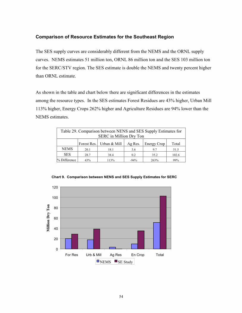
54

Comparison of Resource Estimates for the Southeast Region

The SES supply curves are considerably different from the NEMS and the ORNL supply

curves. NEMS estimates 51 million ton, ORNL 86 million ton and the SES 103 million ton

for the SERC/STV region. The SES estimate is double the NEMS and twenty percent higher

than ORNL estimate.

As shown in the table and chart below there are significant differences in the estimates

among the resource types. In the SES estimates Forest Residues are 43% higher, Urban Mill

113% higher, Energy Crops 262% higher and Agriculture Residues are 94% lower than the

NEMS estimates.

Chart 9. Comparison between NENS and SES Supply Estimates for SERC

0

20

40

60

80

100

120

For Res Urb & Mill Ag Res En Crop Total

Mill

ion

Dry

Ton

NEMS SE Study

Table 29. Comparison between NENS and SES Supply Estimates for SERC in Million Dry Ton

Forest Res. Urban & Mill Ag Res. Energy Crop Total NEMS 20.1 18.1 3.6 9.7 51.5

SES 28.7 38.4 0.2 35.2 102.6

% Difference 43% 113% -94% 263% 99%

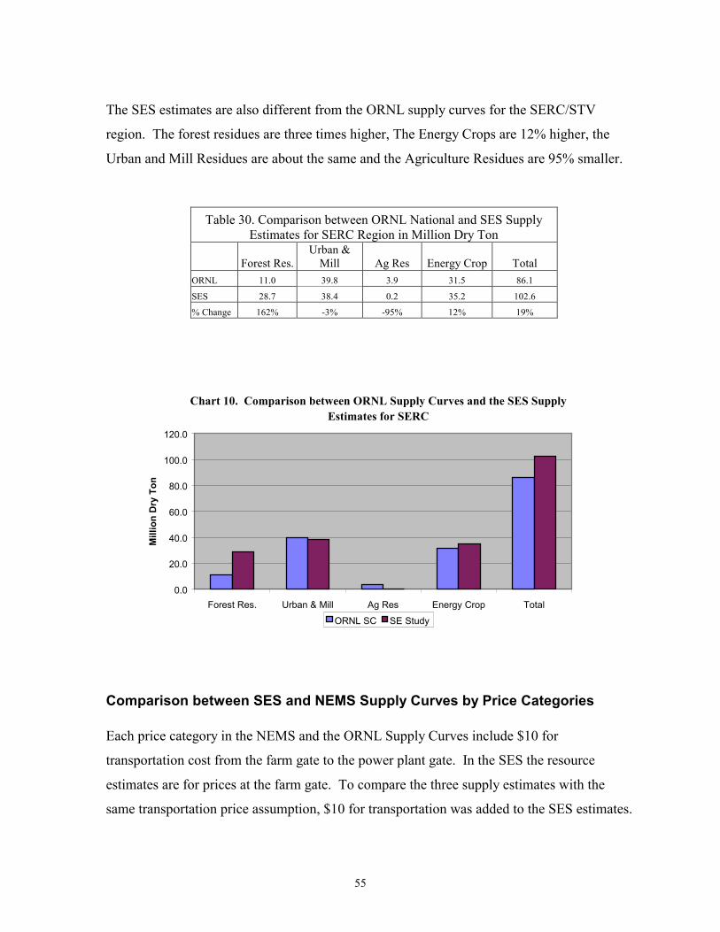
55

The SES estimates are also different from the ORNL supply curves for the SERC/STV

region. The forest residues are three times higher, The Energy Crops are 12% higher, the

Urban and Mill Residues are about the same and the Agriculture Residues are 95% smaller.

Table 30. Comparison between ORNL National and SES Supply Estimates for SERC Region in Million Dry Ton

Forest Res.Urban &

Mill Ag Res Energy Crop Total ORNL 11.0 39.8 3.9 31.5 86.1

SES 28.7 38.4 0.2 35.2 102.6

% Change 162% -3% -95% 12% 19%

Chart 10. Comparison between ORNL Supply Curves and the SES Supply Estimates for SERC

0.0

20.0

40.0

60.0

80.0

100.0

120.0

Forest Res. Urban & Mill Ag Res Energy Crop Total

Mill

ion

Dry

Ton

ORNL SC SE Study

Comparison between SES and NEMS Supply Curves by Price Categories Each price category in the NEMS and the ORNL Supply Curves include $10 for

transportation cost from the farm gate to the power plant gate. In the SES the resource

estimates are for prices at the farm gate. To compare the three supply estimates with the

same transportation price assumption, $10 for transportation was added to the SES estimates.

56

This was accomplished by changing the SES $12.50 category to be $20, the $20 category to

$30, the $30 to $40, the $40 to $50 and the $50 to $60. The change did not affect the total

estimated biomass quantities. The adjustment changed the availability of resources in each

price category for the SES. All supply estimates are in English dry ton.

The differences Between NEMS and the SES estimates are compared in the table below. The

only resources available in the $20 price category for both databases, are in Urban Wood

Waste and Mill Residues. The SES estimates of 906 ton are 80% smaller than NEMS 4,765

ton.

In the $30 price category the total SES resource estimate is 21,753 ton compared to NEMS

9,203 ton. The SES quantities are more than twice the NEMS estimates. SES Forest

Residues are 43% and Urban and Mill Residues 3.5 times higher than NEMS. SES has no

resources while NEMS has 787 ton in Agriculture Residues and 1492 ton in Energy Crops.

In the $40 price category the SES estimate of 57,104 ton is 41% higher than NEMS. Urban

and Mill Residues are 125% higher, Energy Crops 35% higher, and Forest Residues are 14%

higher than NEMS estimates. The SES has no resources while NEMS estimates 3,559 ton in

Agriculture Residues.

The estimate for the $50 and $60 price category follows the same differences with higher

estimates in Forest Residues, Urban and Mill Residues and Energy Crops, and Smaller

estimates in Agriculture Residues in the SES compared with the NEMS estimates.

57

Table 31. Comparison of NEMS and ORNL SES Supply Curves for SERC/STV by Price

(Thousand DT)

Resource Type Forest Residues Urban & Mill Residues Agriculture Residues Price $DT NEMS SES % Change NEMS SES % Change NEMS SES % Change

20 0 0 0 4,765 906 -81% 0 0 0%

30 1,012 1,442 43% 5,912 20,307 244% 787 0 -100% 40 17,384 19,762 14% 11,903 26,827 125% 3,559 0 -100% 50 18,829 27,301 45% 18,017 26,827 49% 3,559 111 -97%

60-115* 20,098 28,745 43% 18,087 38,438 113% 3,559 231 -93%

Resource Type Energy Crop Total Price $DT NEMS SES % Change NEMS SES % Change

20 0 0 0 4,765 906 -81%

30 1,492 0 -100% 9,203 21,749 136% 40 7,794 10,491 35% 40,639 57,080 41% 50 9,703 28,430 193% 50,109 82,699 65%

60-115* 9,703 35,156 262% 51,447 102,570 99%

* $60 for SES and $115 for NEMS

Chart 11. Comparison of Estimated Resources by Price between NEMS and SES for SERC/STV

0

20,000

40,000

60,000

80,000

100,000

120,000

20 30 40 50 60-115*

Price per Ton

Thou

sand

Ton

s

NEMS SES

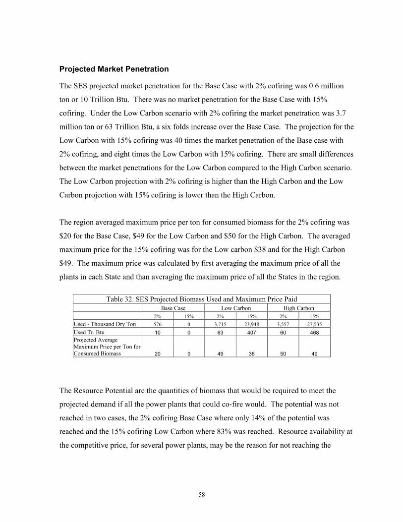
58

Projected Market Penetration

The SES projected market penetration for the Base Case with 2% cofiring was 0.6 million

ton or 10 Trillion Btu. There was no market penetration for the Base Case with 15%

cofiring. Under the Low Carbon scenario with 2% cofiring the market penetration was 3.7

million ton or 63 Trillion Btu, a six folds increase over the Base Case. The projection for the

Low Carbon with 15% cofiring was 40 times the market penetration of the Base case with

2% cofiring, and eight times the Low Carbon with 15% cofiring. There are small differences

between the market penetrations for the Low Carbon compared to the High Carbon scenario.

The Low Carbon projection with 2% cofiring is higher than the High Carbon and the Low

Carbon projection with 15% cofiring is lower than the High Carbon.

The region averaged maximum price per ton for consumed biomass for the 2% cofiring was

$20 for the Base Case, $49 for the Low Carbon and $50 for the High Carbon. The averaged

maximum price for the 15% cofiring was for the Low carbon $38 and for the High Carbon

$49. The maximum price was calculated by first averaging the maximum price of all the

plants in each State and than averaging the maximum price of all the States in the region.

The Resource Potential are the quantities of biomass that would be required to meet the

projected demand if all the power plants that could co-fire would. The potential was not

reached in two cases, the 2% cofiring Base Case where only 14% of the potential was

reached and the 15% cofiring Low Carbon where 83% was reached. Resource availability at

the competitive price, for several power plants, may be the reason for not reaching the

Table 32. SES Projected Biomass Used and Maximum Price Paid Base Case Low Carbon High Carbon 2% 15% 2% 15% 2% 15% Used - Thousand Dry Ton 576 0 3,715 23,948 3,557 27,535 Used Tr. Btu 10 0 63 407 60 468 Projected Average Maximum Price per Ton for Consumed Biomass 20 0 49 38 50 49

59

potential. Even so when comparing the regional resources with the total available or with the

resource availability at the region’s averaged price there appear to be adequate resources to

meet the demand.

Of the availability of resources for the region only one to four percent under the 2% cofiring

and twenty-three to twenty-seven percent under the 15% cofiring, was used.

Table 34. Resource Used Compared with Resource Availability – Thousand Dry Ton Base Case Low Carbon High Carbon

2% 15% 2% 15% 2% 15%

Resource Available 102,627 102,627 102,627 102,627 102,627 102,627

Resource Used 573 0 3,715 23,948 3,557 27,535

% Used 1% 0% 4% 23% 3% 27%

Table 35. Comparison of SES Projected demand and Available Resources by the Averaged Maximum Price of Biomass used

Projection Thousand

Dry Ton Price $DT SES Resource

Estimate % Used

Base Case 2% Cofiring 576 20 906 63%

Low Carbon 15% Cofiring 23,948 40 82,669 42%

Low Carbon 2% Cofiring 3,715 50 102,570 4%

High Carbon 15% Cofiring 27,535 50 102,570 33%

Table 33. SES Resource Used Compared with Resource Potential – Thousand Dry Ton Base Case Low Carbon High Carbon

2% 15% 2% 15% 2% 15%

Region Total Potential 4,194 32,222 3,715 28,906 3,557 27,562

Regional Total Used 573 0 3,715 23,948 3,557 27,535

% Used 14% 0% 100% 83% 100% 100%

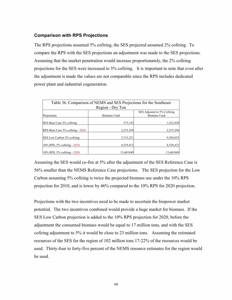
60

Comparison with RPS Projections

The RPS projections assumed 5% cofiring, the SES projected assumed 2% cofiring. To

compare the RPS with the SES projections an adjustment was made to the SES projections.

Assuming that the market penetration would increase proportionately, the 2% cofiring

projections for the SES were increased to 5% cofiring. It is important to note that even after

the adjustment is made the values are not comparable since the RPS includes dedicated

power plant and industrial cogeneration.

Table 36. Comparison of NEMS and SES Projections for the Southeast Region - Dry Ton

Projections Biomass Used SES Adjusted to 5% Cofiring

Biomass Used

SES Base Case 2% cofiring 573,143 1,432,858

RPS Base Case 5% cofiring - 2010 2,235,294 2,235,294

SES Low Carbon 2% cofiring 3,715,221 9,288,053

10% RPS, 5% cofiring - 2010 4,529,412 4,529,412

10% RPS, 5% cofiring - 2020 13,601849 13,601849

Assuming the SES would co-fire at 5% after the adjustment of the SES Reference Case is

56% smaller than the NEMS Reference Case projections. The SES projection for the Low

Carbon assuming 5% cofiring is twice the projected biomass use under the 10% RPS

projection for 2010, and is lower by 46% compared to the 10% RPS for 2020 projection.

Projections with the two incentives need to be made to ascertain the biopower market

potential. The two incentives combined would provide a huge market for biomass. If the

SES Low Carbon projection is added to the 10% RPS projection for 2020, before the

adjustment the consumed biomass would be equal to 17 million tons, and with the SES

cofiring adjustment to 5% it would be close to 23 million tons. Assuming the estimated

resources of the SES for the region of 102 million tons 17-22% of the resources would be

used. Thirty-four to forty-five percent of the NEMS resource estimates for the region would

be used.

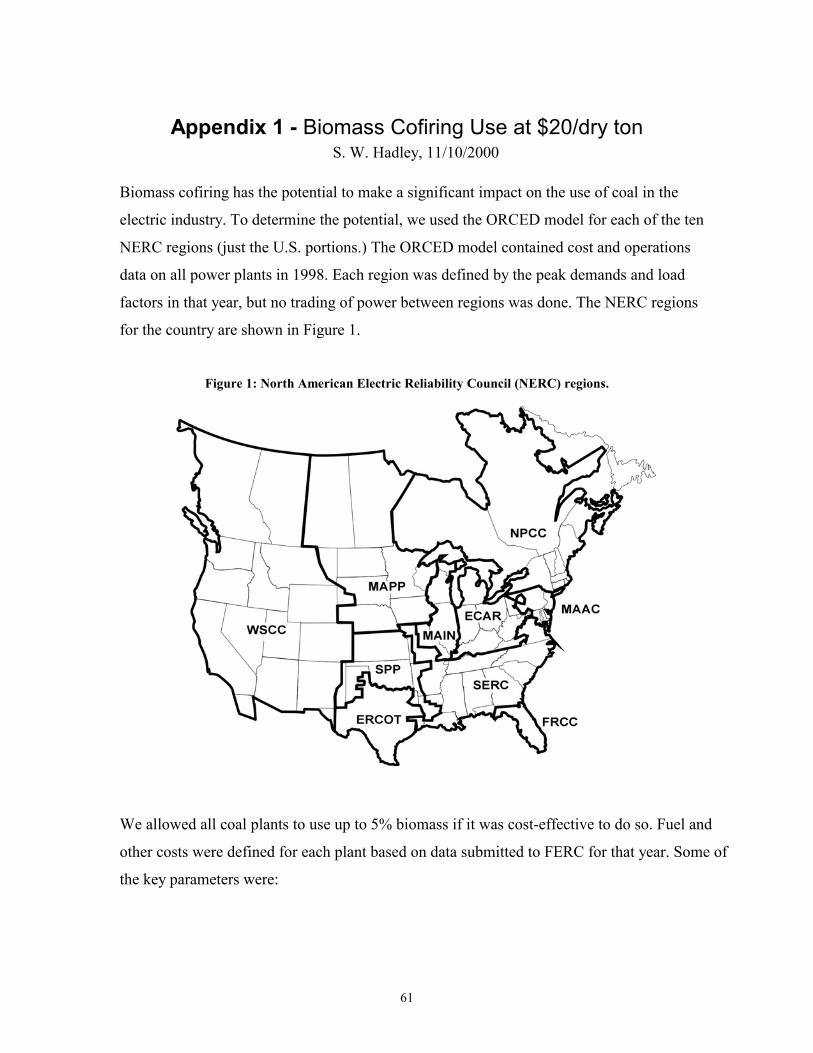
61

Appendix 1 - Biomass Cofiring Use at $20/dry ton S. W. Hadley, 11/10/2000

Biomass cofiring has the potential to make a significant impact on the use of coal in the

electric industry. To determine the potential, we used the ORCED model for each of the ten

NERC regions (just the U.S. portions.) The ORCED model contained cost and operations

data on all power plants in 1998. Each region was defined by the peak demands and load

factors in that year, but no trading of power between regions was done. The NERC regions

for the country are shown in Figure 1.

Figure 1: North American Electric Reliability Council (NERC) regions.

We allowed all coal plants to use up to 5% biomass if it was cost-effective to do so. Fuel and

other costs were defined for each plant based on data submitted to FERC for that year. Some of

the key parameters were:

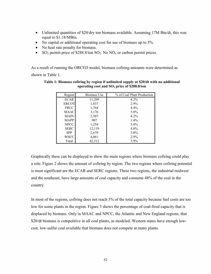
62

• Unlimited quantities of $20/dry ton biomass available. Assuming 17M Btu/dt, this was equal to $1.18/MBtu.

• No capital or additional operating cost for use of biomass up to 5%. • No heat rate penalty for biomass. • SO2 permit price of $288.8/ton SO2. No NOx or carbon permit prices.

As a result of running the ORCED model, biomass cofiring amounts were determined as

shown in Table 1.

Table 1: Biomass cofiring by region if unlimited supply at $20/dt with no additional operating cost and SO2 price of $288.8/ton

Region Biomass Use % of Coal Plant Production ECAR 11,209 4.2%

ERCOT 1,837 2.9% FRCC 1,764 4.4% MAAC 3,176 5.0% MAIN 3,307 4.2% MAPP 907 1.4% NPCC 1,254 5.0% SERC 12,119 4.8% SPP 2,679 3.0%

WSCC 4,061 2.9% Total 42,312 3.9%

Graphically these can be displayed to show the main regions where biomass cofiring could play

a role. Figure 2 shows the amount of cofiring by region. The two regions where cofiring potential

is most significant are the ECAR and SERC regions. These two regions, the industrial midwest

and the southeast, have large amounts of coal capacity and consume 48% of the coal in the

country.

In most of the regions, cofiring does not reach 5% of the total capacity because fuel costs are too

low for some plants in the region. Figure 3 shows the percentage of coal-fired capacity that is

displaced by biomass. Only in MAAC and NPCC, the Atlantic and New England regions, that

$20/dt biomass is competitive in all coal plants, as modeled. Western states have enough low-

cost, low-sulfur coal available that biomass does not compete at many plants.

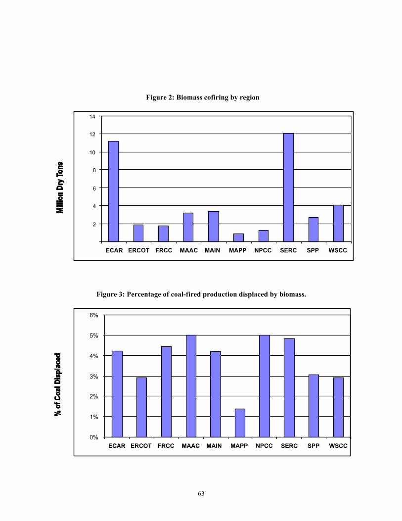
63

Figure 2: Biomass cofiring by region

2

4

6

8

10

12

14

ECAR ERCOT FRCC MAAC MAIN MAPP NPCC SERC SPP WSCC

Figure 3: Percentage of coal-fired production displaced by biomass.

0%

1%

2%

3%

4%

5%

6%

ECAR ERCOT FRCC MAAC MAIN MAPP NPCC SERC SPP WSCC

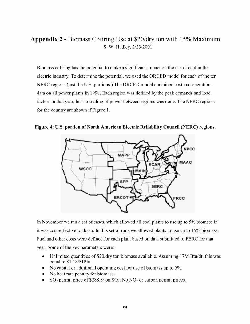
64

Appendix 2 - Biomass Cofiring Use at $20/dry ton with 15% Maximum S. W. Hadley, 2/23/2001

Biomass cofiring has the potential to make a significant impact on the use of coal in the

electric industry. To determine the potential, we used the ORCED model for each of the ten

NERC regions (just the U.S. portions.) The ORCED model contained cost and operations

data on all power plants in 1998. Each region was defined by the peak demands and load

factors in that year, but no trading of power between regions was done. The NERC regions

for the country are shown if Figure 1.

Figure 4: U.S. portion of North American Electric Reliability Council (NERC) regions.

In November we ran a set of cases, which allowed all coal plants to use up to 5% biomass if

it was cost-effective to do so. In this set of runs we allowed plants to use up to 15% biomass.

Fuel and other costs were defined for each plant based on data submitted to FERC for that

year. Some of the key parameters were:

• Unlimited quantities of $20/dry ton biomass available. Assuming 17M Btu/dt, this was equal to $1.18/MBtu.

• No capital or additional operating cost for use of biomass up to 5%. • No heat rate penalty for biomass. • SO2 permit price of $288.8/ton SO2. No NOx or carbon permit prices.

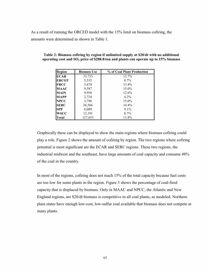
65

As a result of running the ORCED model with the 15% limit on biomass cofiring, the

amounts were determined as shown in Table 1.

Table 2: Biomass cofiring by region if unlimited supply at $20/dt with no additional operating cost and SO2 price of $288.8/ton and plants can operate up to 15% biomass

Region Biomass Use % of Coal Plant Production ECAR 33,733 12.7% ERCOT 5,535 8.7% FRCC 5,474 13.4% MAAC 9,587 15.0% MAIN 9,958 12.6% MAPP 2,724 4.2% NPCC 3,796 15.0% SERC 36,566 14.4% SPP 8,089 9.1% WSCC 12,191 8.7% Total 127,653 11.8%

Graphically these can be displayed to show the main regions where biomass cofiring could

play a role. Figure 2 shows the amount of cofiring by region. The two regions where cofiring

potential is most significant are the ECAR and SERC regions. These two regions, the

industrial midwest and the southeast, have large amounts of coal capacity and consume 48%

of the coal in the country.

In most of the regions, cofiring does not reach 15% of the total capacity because fuel costs

are too low for some plants in the region. Figure 3 shows the percentage of coal-fired

capacity that is displaced by biomass. Only in MAAC and NPCC, the Atlantic and New

England regions, are $20/dt biomass is competitive in all coal plants, as modeled. Northern

plain states have enough low-cost, low-sulfur coal available that biomass does not compete at

many plants.

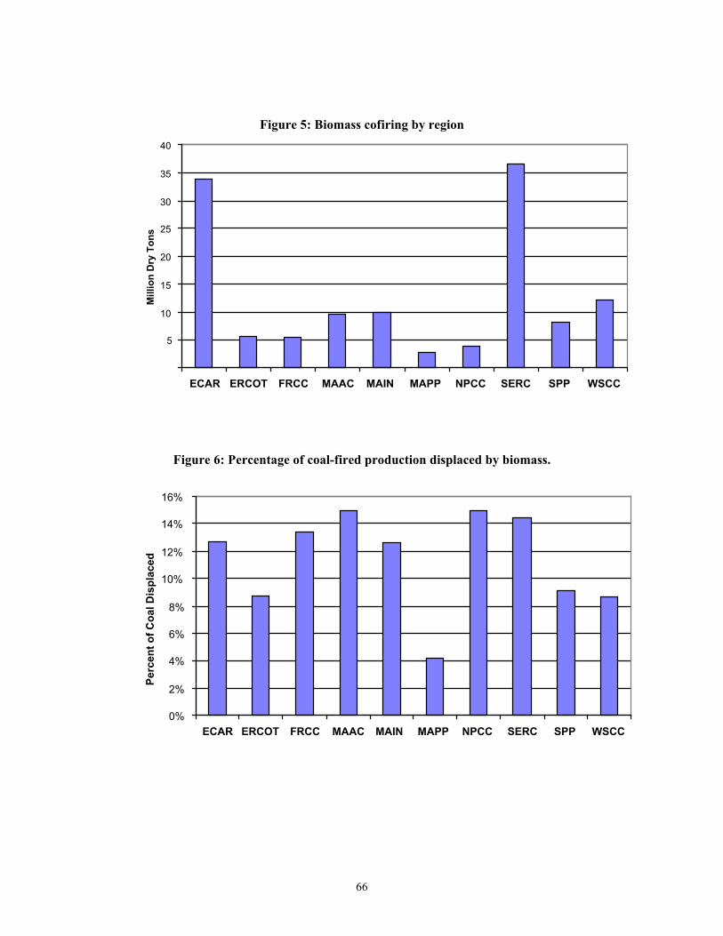
66

Figure 5: Biomass cofiring by region

5

10

15

20

25

30

35

40

ECAR ERCOT FRCC MAAC MAIN MAPP NPCC SERC SPP WSCC

Mill

ion

Dry

Ton

s

Figure 6: Percentage of coal-fired production displaced by biomass.

0%

2%

4%

6%

8%

10%

12%

14%

16%

ECAR ERCOT FRCC MAAC MAIN MAPP NPCC SERC SPP WSCC

Perc

ent o

f Coa

l Dis

plac

ed

67

Appendix 3 - Potential Market Penetration of Biomass Co-firing, Interim Report

MEMORANDUM January 31, 2001

TO: Lynn Wright, Bob Perlack, ORNL

CC: Jacob Kaminsky

FROM: Juanita Haydel, Bishal Thapa, John Leahy, ICF Consulting

SUBJECT: Potential Market Penetration of Biomass Co-firing, Interim Report Subcontract Number 400000496

This memo summarizes the results of the study on the potential market penetration of

biomass co-firing. The study used ICF’s Integrated Planning Model (IPMTM) to evaluate the

potential penetration of biomass co-firing in existing coal-fired units in two scenarios that

assumed unlimited biomass supply to all coal generating units at a price of $20/dry ton. The

two scenarios allowed coal plants to co-fire at five percent and fifteen percent. Both the

scenarios assumed that there would be no incremental investment or operating costs incurred

as a result of retrofitting to biomass co-firing.

The study analyzed the entire U.S. electric power system, capturing regional distinctions,

over a time horizon between 2005 and 2020. Results from the scenarios were compared to a

business as usual (BAU) base case that did not include biomass co-firing. The remainder of

this memorandum describes the following:

1. Study methodology and assumptions, 2. Scenarios analyzed, 3. Results, and 4. Conclusions.

1. Study Methodology and Assumptions This section describes the modeling tool and provides references to the assumptions used for

this analysis.

68

The Modeling Tool

IPMTM is a multi-region linear programming model that determines the least-cost operation

of the electric power system to meet a specified electricity demand. IPMTM decides upon the

operation of the existing system and chooses new units and retrofit options based on the

criteria of meeting demand at least-cost subject to constraints imposed. Constraints include

unit operating constraints, emissions caps, interregional transmission limits, and regional

reserve margins, among others. The model draws on a database containing detailed

information on the characteristics of each utility boiler and generating unit in the U.S. For

modeling purposes, these units are aggregated into model plants of similar characteristics.

The model has a comprehensive retrofit structure that allows modifications (environmental

and other) to existing units based on economics. IPMTM structurally models biomass co-firing

by substituting the allowed percentage of coal fuel (on a Btu basis) with biomass fuel. In

IPMTM, plants select biomass co-firing only if it is economically more attractive than the

other options.

IPMTM projects capacity expansion and dispatch for generations into the future by selecting

options that will meet electric demand at least cost to the overall power system. Ordinarily

this will simply mean dispatching those existing units that have the least variable costs and

building new units or retrofitting existing units in the way that will yield the lowest cost to

meet growing electricity demand. If the scenario includes an environmental constraint, then

the model considers retrofit, new build or fuel switching options that will not only meet

electricity demand but also stay within emissions limits prescribed by the environmental

constraint.

For this study, the U.S. electric system was modeled as twenty-one power markets as

illustrated in Figure I below. These regions correspond in most cases to the regions and sub-

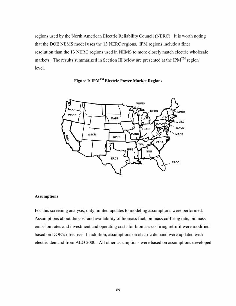
69

regions used by the North American Electric Reliability Council (NERC). It is worth noting

that the DOE NEMS model uses the 13 NERC regions. IPM regions include a finer

resolution than the 13 NERC regions used in NEMS to more closely match electric wholesale

markets. The results summarized in Section III below are presented at the IPMTM region

level.

Figure I: IPMTM Electric Power Market Regions

Assumptions

For this screening analysis, only limited updates to modeling assumptions were performed.

Assumptions about the cost and availability of biomass fuel, biomass co-firing rate, biomass

emission rates and investment and operating costs for biomass co-firing retrofit were modified

based on DOE’s directive. In addition, assumptions on electric demand were updated with

electric demand from AEO 2000. All other assumptions were based on assumptions developed

CN

V SPPN

ERCT

NENG

LILC

UPNY

FRCC

WUMS

MECS

MACS

MACEMACW

SOUSPPS

WSCP

WSCR

MAPP

TVA

ECAO

MANO

VACA

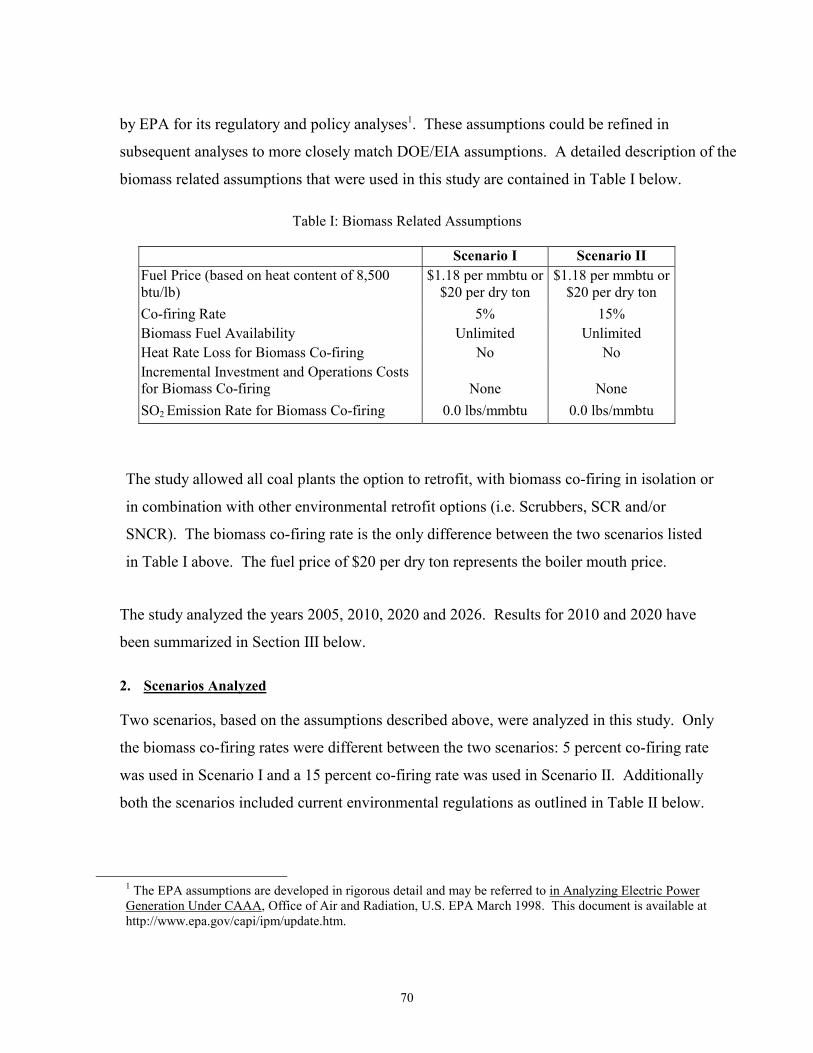
70

by EPA for its regulatory and policy analyses1. These assumptions could be refined in

subsequent analyses to more closely match DOE/EIA assumptions. A detailed description of the

biomass related assumptions that were used in this study are contained in Table I below.

Table I: Biomass Related Assumptions

Scenario I Scenario II Fuel Price (based on heat content of 8,500 btu/lb)

$1.18 per mmbtu or $20 per dry ton

$1.18 per mmbtu or $20 per dry ton

Co-firing Rate 5% 15% Biomass Fuel Availability Unlimited Unlimited Heat Rate Loss for Biomass Co-firing No No Incremental Investment and Operations Costs for Biomass Co-firing

None

None

SO2 Emission Rate for Biomass Co-firing 0.0 lbs/mmbtu 0.0 lbs/mmbtu

The study allowed all coal plants the option to retrofit, with biomass co-firing in isolation or

in combination with other environmental retrofit options (i.e. Scrubbers, SCR and/or

SNCR). The biomass co-firing rate is the only difference between the two scenarios listed

in Table I above. The fuel price of $20 per dry ton represents the boiler mouth price.

The study analyzed the years 2005, 2010, 2020 and 2026. Results for 2010 and 2020 have

been summarized in Section III below.

2. Scenarios Analyzed Two scenarios, based on the assumptions described above, were analyzed in this study. Only

the biomass co-firing rates were different between the two scenarios: 5 percent co-firing rate

was used in Scenario I and a 15 percent co-firing rate was used in Scenario II. Additionally

both the scenarios included current environmental regulations as outlined in Table II below.

1 The EPA assumptions are developed in rigorous detail and may be referred to in Analyzing Electric Power Generation Under CAAA, Office of Air and Radiation, U.S. EPA March 1998. This document is available at http://www.epa.gov/capi/ipm/update.htm.

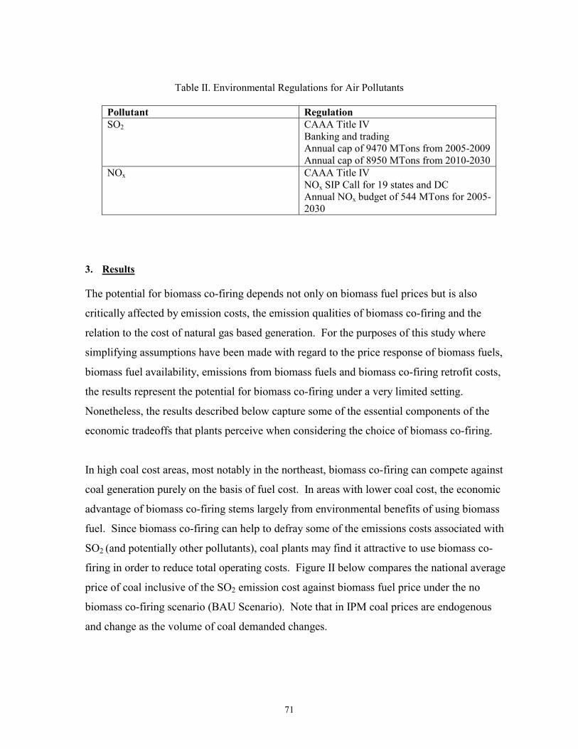
71

Table II. Environmental Regulations for Air Pollutants

Pollutant Regulation SO2 CAAA Title IV

Banking and trading Annual cap of 9470 MTons from 2005-2009 Annual cap of 8950 MTons from 2010-2030

NOx CAAA Title IV NOx SIP Call for 19 states and DC Annual NOx budget of 544 MTons for 2005-2030

3. Results

The potential for biomass co-firing depends not only on biomass fuel prices but is also

critically affected by emission costs, the emission qualities of biomass co-firing and the

relation to the cost of natural gas based generation. For the purposes of this study where

simplifying assumptions have been made with regard to the price response of biomass fuels,

biomass fuel availability, emissions from biomass fuels and biomass co-firing retrofit costs,

the results represent the potential for biomass co-firing under a very limited setting.

Nonetheless, the results described below capture some of the essential components of the

economic tradeoffs that plants perceive when considering the choice of biomass co-firing.

In high coal cost areas, most notably in the northeast, biomass co-firing can compete against

coal generation purely on the basis of fuel cost. In areas with lower coal cost, the economic

advantage of biomass co-firing stems largely from environmental benefits of using biomass

fuel. Since biomass co-firing can help to defray some of the emissions costs associated with

SO2 (and potentially other pollutants), coal plants may find it attractive to use biomass co-

firing in order to reduce total operating costs. Figure II below compares the national average

price of coal inclusive of the SO2 emission cost against biomass fuel price under the no

biomass co-firing scenario (BAU Scenario). Note that in IPM coal prices are endogenous

and change as the volume of coal demanded changes.

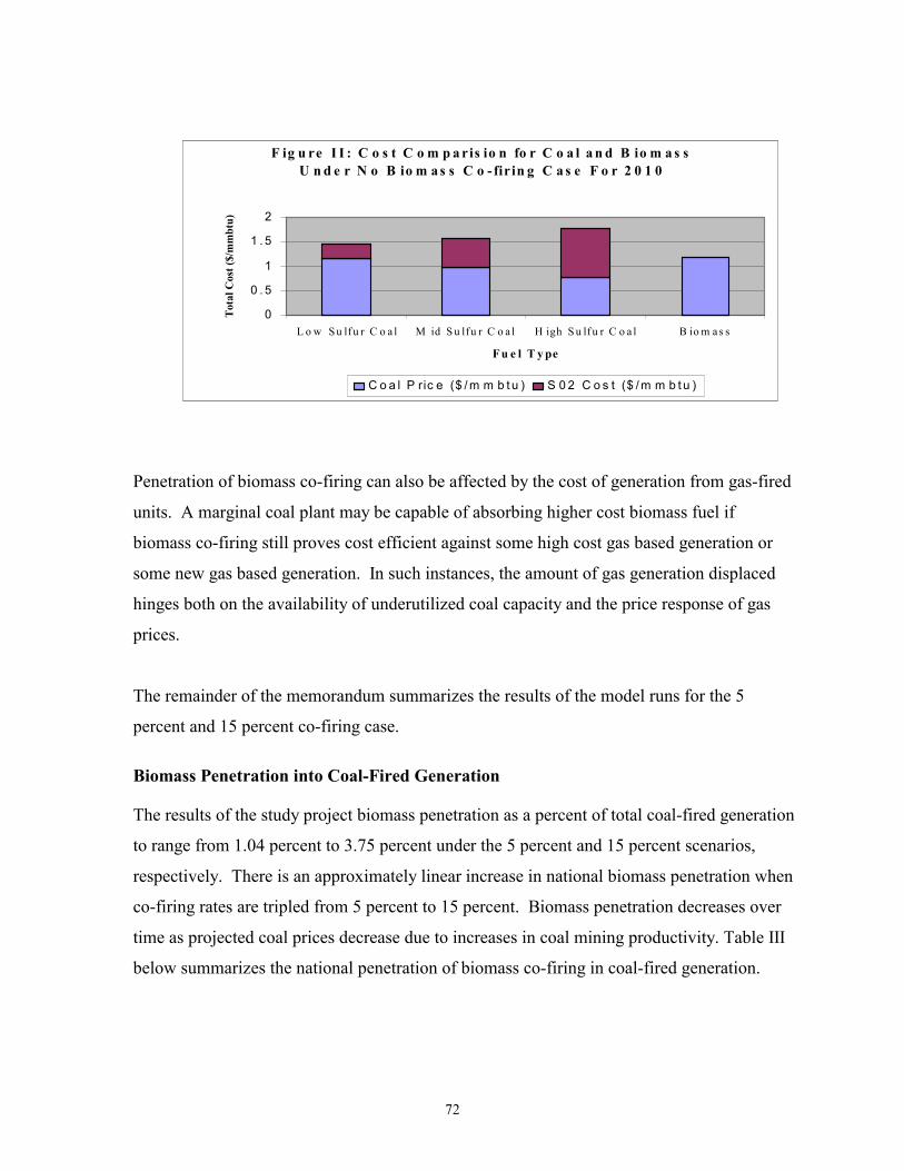
72

Penetration of biomass co-firing can also be affected by the cost of generation from gas-fired

units. A marginal coal plant may be capable of absorbing higher cost biomass fuel if

biomass co-firing still proves cost efficient against some high cost gas based generation or

some new gas based generation. In such instances, the amount of gas generation displaced

hinges both on the availability of underutilized coal capacity and the price response of gas

prices.

The remainder of the memorandum summarizes the results of the model runs for the 5

percent and 15 percent co-firing case.

Biomass Penetration into Coal-Fired Generation The results of the study project biomass penetration as a percent of total coal-fired generation

to range from 1.04 percent to 3.75 percent under the 5 percent and 15 percent scenarios,

respectively. There is an approximately linear increase in national biomass penetration when

co-firing rates are tripled from 5 percent to 15 percent. Biomass penetration decreases over

time as projected coal prices decrease due to increases in coal mining productivity. Table III

below summarizes the national penetration of biomass co-firing in coal-fired generation.

F ig u re I I : C o s t C o m p a ris io n fo r C o a l a n d B io m a s s U n d e r N o B io m a s s C o - fir in g C a s e F o r 2 0 1 0

0

0 . 5

1

1 . 5

2

L o w S u lf u r C o a l M id S u lfu r C o a l H igh S u lf u r C o a l B io m a s s

Fu e l T y pe

Tot

al C

ost (

$/m

mbt

u)

C o a l P ric e ($ / m m b t u ) S 0 2 C o s t ($ / m m b t u )

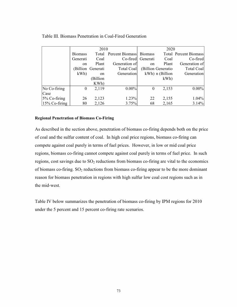
73

Table III. Biomass Penetration in Coal-Fired Generation

2010 2020 Biomass

Generation

(Billion kWh)

Total Coal Plant

Generation

(Billion KWh)

Percent Biomass Co-fired

Generation of Total Coal Generation

Biomass Generati

on (Billion

kWh)

Total Coal Plant

Generation (Billion

kWh)

Percent Biomass Co-fired

Generation of Total Coal Generation

No Co-firing Case

0 2,119 0.00% 0 2,153 0.00%

5% Co-firing 26 2,123 1.23% 22 2,155 1.04%15% Co-firing 80 2,126 3.75% 68 2,165 3.14%

Regional Penetration of Biomass Co-Firing As described in the section above, penetration of biomass co-firing depends both on the price

of coal and the sulfur content of coal. In high coal price regions, biomass co-firing can

compete against coal purely in terms of fuel prices. However, in low or mid coal price

regions, biomass co-firing cannot compete against coal purely in terms of fuel price. In such

regions, cost savings due to SO2 reductions from biomass co-firing are vital to the economics

of biomass co-firing. SO2 reductions from biomass co-firing appear to be the more dominant

reason for biomass penetration in regions with high sulfur low coal cost regions such as in

the mid-west.

Table IV below summarizes the penetration of biomass co-firing by IPM regions for 2010

under the 5 percent and 15 percent co-firing rate scenarios.

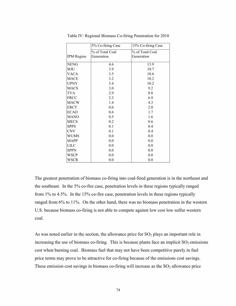
74

Table IV: Regional Biomass Co-firing Penetration for 2010

5% Co-firing Case 15% Co-firing Case

IPM Region

% of Total Coal Generation

% of Total Coal Generation

NENG 4.6 13.9 SOU 3.9 10.7 VACA 3.5 10.6 MACE 3.2 10.2 UPNY 3.4 10.2 MACS 3.0 9.2 TVA 2.9 8.8 FRCC 2.3 6.9 MACW 1.4 4.3 ERCT 0.0 2.0 ECAO 0.6 1.7 MANO 0.5 1.6 MECS 0.2 0.6 SPPS 0.1 0.4 CNV 0.1 0.4 WUMS 0.0 0.0 MAPP 0.0 0.0 LILC 0.0 0.0 SPPN 0.0 0.0 WSCP 0.0 0.0 WSCR 0.0 0.0

The greatest penetration of biomass co-firing into coal-fired generation is in the northeast and

the southeast. In the 5% co-fire case, penetration levels in these regions typically ranged

from 1% to 4.5%. In the 15% co-fire case, penetration levels in these regions typically

ranged from 6% to 11%. On the other hand, there was no biomass penetration in the western

U.S. because biomass co-firing is not able to compete against low cost low sulfur western

coal.

As was noted earlier in the section, the allowance price for SO2 plays an important role in

increasing the use of biomass co-firing. This is because plants face an implicit SO2 emissions

cost when burning coal. Biomass fuel that may not have been competitive purely in fuel

price terms may prove to be attractive for co-firing because of the emissions cost savings.

These emission cost savings in biomass co-firing will increase as the SO2 allowance price

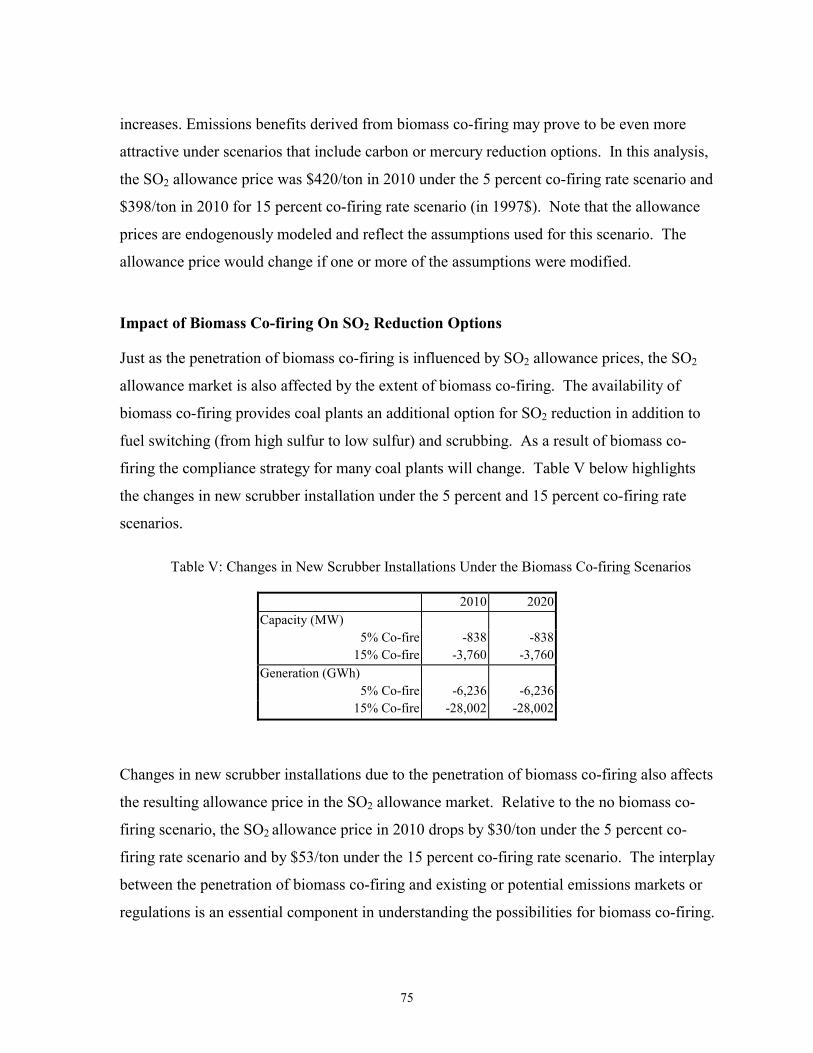
75

increases. Emissions benefits derived from biomass co-firing may prove to be even more

attractive under scenarios that include carbon or mercury reduction options. In this analysis,

the SO2 allowance price was $420/ton in 2010 under the 5 percent co-firing rate scenario and

$398/ton in 2010 for 15 percent co-firing rate scenario (in 1997$). Note that the allowance

prices are endogenously modeled and reflect the assumptions used for this scenario. The

allowance price would change if one or more of the assumptions were modified.

Impact of Biomass Co-firing On SO2 Reduction Options

Just as the penetration of biomass co-firing is influenced by SO2 allowance prices, the SO2

allowance market is also affected by the extent of biomass co-firing. The availability of

biomass co-firing provides coal plants an additional option for SO2 reduction in addition to

fuel switching (from high sulfur to low sulfur) and scrubbing. As a result of biomass co-

firing the compliance strategy for many coal plants will change. Table V below highlights

the changes in new scrubber installation under the 5 percent and 15 percent co-firing rate

scenarios.

Table V: Changes in New Scrubber Installations Under the Biomass Co-firing Scenarios

2010 2020Capacity (MW)

5% Co-fire -838 -838 15% Co-fire -3,760 -3,760

Generation (GWh) 5% Co-fire -6,236 -6,236 15% Co-fire -28,002 -28,002

Changes in new scrubber installations due to the penetration of biomass co-firing also affects

the resulting allowance price in the SO2 allowance market. Relative to the no biomass co-

firing scenario, the SO2 allowance price in 2010 drops by $30/ton under the 5 percent co-

firing rate scenario and by $53/ton under the 15 percent co-firing rate scenario. The interplay

between the penetration of biomass co-firing and existing or potential emissions markets or

regulations is an essential component in understanding the possibilities for biomass co-firing.

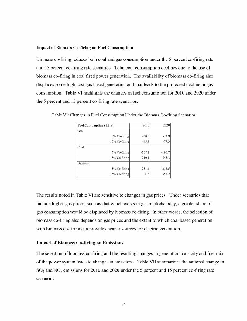
76

Impact of Biomass Co-firing on Fuel Consumption

Biomass co-firing reduces both coal and gas consumption under the 5 percent co-firing rate

and 15 percent co-firing rate scenarios. Total coal consumption declines due to the use of

biomass co-firing in coal fired power generation. The availability of biomass co-firing also

displaces some high cost gas based generation and that leads to the projected decline in gas

consumption. Table VI highlights the changes in fuel consumption for 2010 and 2020 under

the 5 percent and 15 percent co-firing rate scenarios.

Table VI: Changes in Fuel Consumption Under the Biomass Co-firing Scenarios

Fuel Consumption (TBtu) 2010 2020

Gas 5% Co-firing -30.5 -13.9

15% Co-firing -45.9 -77.3

Coal 5% Co-firing -207.1 -196.7

15% Co-firing -710.1 -545.3

Biomass

5% Co-firing 254.6 216.515% Co-firing 778 657.2

The results noted in Table VI are sensitive to changes in gas prices. Under scenarios that

include higher gas prices, such as that which exists in gas markets today, a greater share of

gas consumption would be displaced by biomass co-firing. In other words, the selection of

biomass co-firing also depends on gas prices and the extent to which coal based generation

with biomass co-firing can provide cheaper sources for electric generation.

Impact of Biomass Co-firing on Emissions

The selection of biomass co-firing and the resulting changes in generation, capacity and fuel mix

of the power system leads to changes in emissions. Table VII summarizes the national change in

SO2 and NOx emissions for 2010 and 2020 under the 5 percent and 15 percent co-firing rate

scenarios.

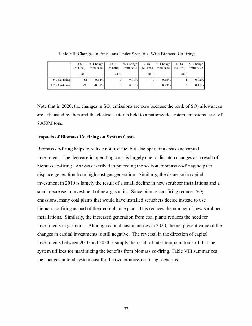
77

Table VII: Changes in Emissions Under Scenarios With Biomass Co-firing

SO2 (MTons)

% Change from Base

SO2 (MTons)

% Change from Base

NOX (MTons)

% Change from Base

NOX (MTons)

% Change from Base

2010 2020 2010 2020

5% Co-firing -61 -0.64% 0 0.00% 7 0.18% 1 0.02%15% Co-firing -90 -0.95% 0 0.00% 10 0.23% 5 0.11%

Note that in 2020, the changes in SO2 emissions are zero because the bank of SO2 allowances

are exhausted by then and the electric sector is held to a nationwide system emissions level of

8,950M tons.

Impacts of Biomass Co-firing on System Costs

Biomass co-firing helps to reduce not just fuel but also operating costs and capital

investment. The decrease in operating costs is largely due to dispatch changes as a result of

biomass co-firing. As was described in preceding the section, biomass co-firing helps to

displace generation from high cost gas generation. Similarly, the decrease in capital

investment in 2010 is largely the result of a small decline in new scrubber installations and a

small decrease in investment of new gas units. Since biomass co-firing reduces SO2

emissions, many coal plants that would have installed scrubbers decide instead to use

biomass co-firing as part of their compliance plan. This reduces the number of new scrubber

installations. Similarly, the increased generation from coal plants reduces the need for

investments in gas units. Although capital cost increases in 2020, the net present value of the

changes in capital investments is still negative. The reversal in the direction of capital

investments between 2010 and 2020 is simply the result of inter-temporal tradeoff that the

system utilizes for maximizing the benefits from biomass co-firing. Table VIII summarizes

the changes in total system cost for the two biomass co-firing scenarios.

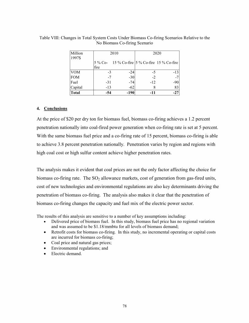
78

Table VIII: Changes in Total System Costs Under Biomass Co-firing Scenarios Relative to the No Biomass Co-firing Scenario

Million 1997$

2010 2020

5 % Co-fire

15 % Co-fire 5 % Co-fire 15 % Co-fire

VOM -3 -24 -5 -13 FOM -7 -30 -2 -7 Fuel -31 -74 -12 -90 Capital -13 -62 8 83 Total -54 -190 -11 -27

4. Conclusions

At the price of $20 per dry ton for biomass fuel, biomass co-firing achieves a 1.2 percent

penetration nationally into coal-fired power generation when co-firing rate is set at 5 percent.

With the same biomass fuel price and a co-firing rate of 15 percent, biomass co-firing is able

to achieve 3.8 percent penetration nationally. Penetration varies by region and regions with

high coal cost or high sulfur content achieve higher penetration rates.

The analysis makes it evident that coal prices are not the only factor affecting the choice for

biomass co-firing rate. The SO2 allowance markets, cost of generation from gas-fired units,

cost of new technologies and environmental regulations are also key determinants driving the

penetration of biomass co-firing. The analysis also makes it clear that the penetration of

biomass co-firing changes the capacity and fuel mix of the electric power sector.

The results of this analysis are sensitive to a number of key assumptions including: • Delivered price of biomass fuel. In this study, biomass fuel price has no regional variation

and was assumed to be $1.18/mmbtu for all levels of biomass demand; • Retrofit costs for biomass co-firing. In this study, no incremental operating or capital costs

are incurred for biomass co-firing; • Coal price and natural gas prices; • Environmental regulations; and • Electric demand.

79

Appendix 4 - Results of Phase II of Study on Potential Market Penetration of Biomass Co-firing

July 19, 2001

TO: Lynn Wright, Bob Perlack, ORNL

CC: Jacob Kaminsky

FROM: Bishal Thapa, John Leahy, ICF Consulting

SUBJECT: Results of Phase II of Study on Potential Market Penetration of Biomass Co-firing Subcontract Number 400000496

This memo summarizes the results of Phase II of the study on the potential market

penetration of biomass co-firing. On January 31, 2001 ICF completed Phase I of the study

and a memorandum containing the results was provided by ICF to ORNL (Wright and

Perlack).

Both phases of the study used ICF’s Integrated Planning Model (IPM®) to evaluate the

potential penetration of biomass co-firing in existing coal-fired units. Both phases of the

study assumed that an unlimited supply of biomass fuel would be available to all coal-fired

generating units at a price of $20/dry ton for biomass co-firing. As in the previous phase of

the study, this analysis included two scenarios. Both scenarios in this analysis allowed

biomass co-firing at coal-fired plants but, unlike the previous phase of the study, included

explicit assumptions on capital cost and FO&M cost for biomass co-firing along with

efficiency losses for biomass co-firing.

Phase I of the study showed some penetration of biomass co-firing in coal-fired generation.

The Phase I analysis, which assumed biomass fuel price of $20 per dry ton with no capital

cost, FO&M cost or efficiency losses for biomass co-firing retrofits, resulted in a 1.2% and

3.8% penetration nationally for the scenarios with 5% and 15% co-firing rates respectively.

80

In Phase II, the findings suggest that biomass co-firing will not be economically competitive

against other generating technologies given the capital cost, FO&M cost, efficiency losses

and biomass fuel price assumed in this analysis. Biomass co-firing fails to penetrate

generation markets because the incremental cost of building and operating the biomass co-

firing system more than offsets the fuel and/or emission cost savings.

This study analyzed the entire U.S. electric power system, capturing regional distinctions,

over a time horizon between 2005 and 2020. The remainder of this memorandum describes

the following:

5. Study methodology and assumptions, 6. Scenarios analyzed, 7. Results, and 8. Conclusions.

For the remainder of this memo, unless otherwise noted this analysis refers to Phase II of the

study.

5. Study Methodology and Assumptions

Assumptions

For this analysis, DOE provided the assumptions about the biomass co-firing rate, capital

cost, fixed operation and maintenance cost (FO&M), efficiency losses and biomass fuel

prices. Table I below provides a summary of the biomass related assumptions used in this

analysis.

Table I: Biomass Related Assumptions Scenario I Scenario II

Fuel Price (based on heat content of 8,500 Btu/lb)

$1.18 per mmBtu or $20 per dry ton

$1.18 per mmBtu or $20 per dry ton

Co-firing Rate 5% 15% Biomass Fuel Availability Unlimited Unlimited Heat Rate Loss for Biomass Co-firing 1% 2% Incremental Capital Cost for retrofit ($/kW) 2.5 30 Incremental FOM Cost for retrofit ($/kW-yr) 0.35 1.5 SO2 Emission Rate for Biomass Co-firing 0.0 lbs/mmBtu 0.0 lbs/mmBtu

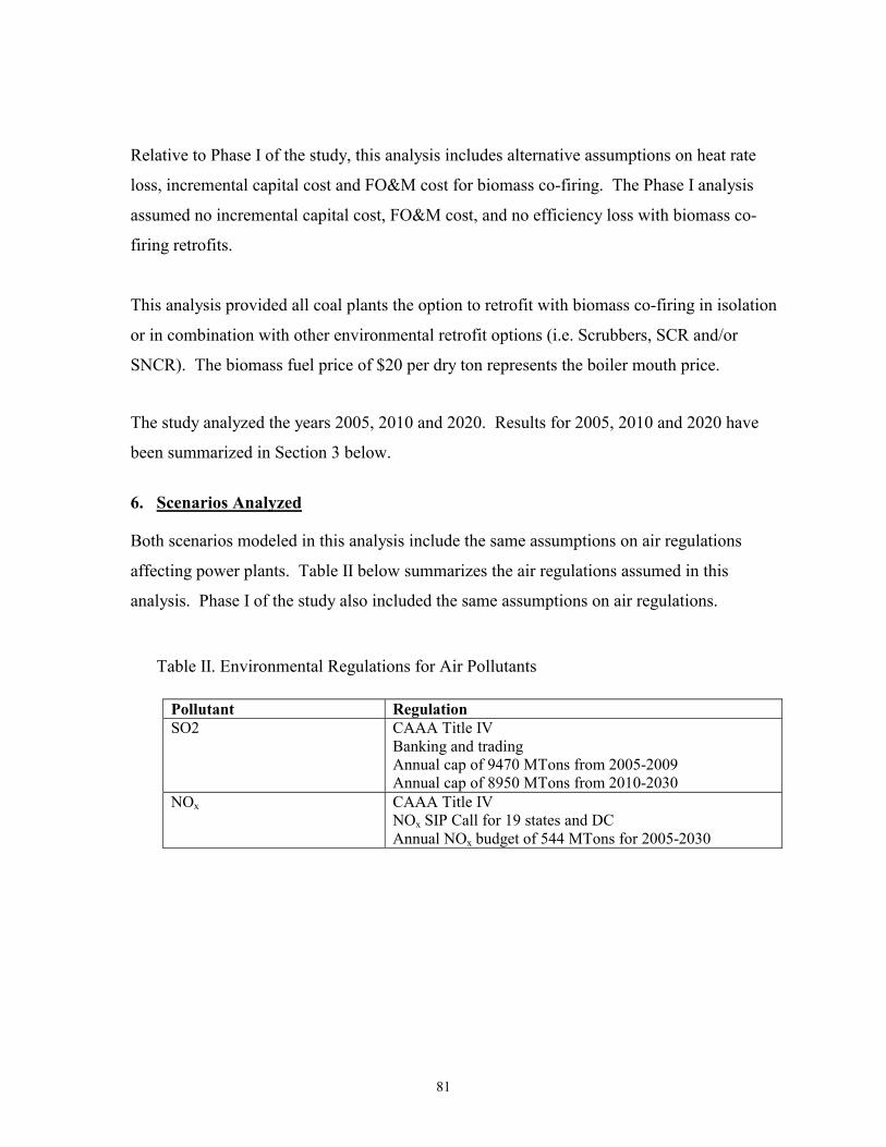
81

Relative to Phase I of the study, this analysis includes alternative assumptions on heat rate

loss, incremental capital cost and FO&M cost for biomass co-firing. The Phase I analysis

assumed no incremental capital cost, FO&M cost, and no efficiency loss with biomass co-

firing retrofits.

This analysis provided all coal plants the option to retrofit with biomass co-firing in isolation

or in combination with other environmental retrofit options (i.e. Scrubbers, SCR and/or

SNCR). The biomass fuel price of $20 per dry ton represents the boiler mouth price.

The study analyzed the years 2005, 2010 and 2020. Results for 2005, 2010 and 2020 have

been summarized in Section 3 below.

6. Scenarios Analyzed

Both scenarios modeled in this analysis include the same assumptions on air regulations

affecting power plants. Table II below summarizes the air regulations assumed in this

analysis. Phase I of the study also included the same assumptions on air regulations.

Table II. Environmental Regulations for Air Pollutants

Pollutant Regulation SO2 CAAA Title IV

Banking and trading Annual cap of 9470 MTons from 2005-2009 Annual cap of 8950 MTons from 2010-2030

NOx CAAA Title IV NOx SIP Call for 19 states and DC Annual NOx budget of 544 MTons for 2005-2030

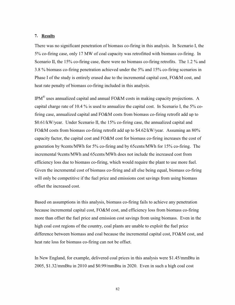
82

7. Results

There was no significant penetration of biomass co-firing in this analysis. In Scenario I, the

5% co-firing case, only 17 MW of coal capacity was retrofitted with biomass co-firing. In

Scenario II, the 15% co-firing case, there were no biomass co-firing retrofits. The 1.2 % and

3.8 % biomass co-firing penetration achieved under the 5% and 15% co-firing scenarios in

Phase I of the study is entirely erased due to the incremental capital cost, FO&M cost, and

heat rate penalty of biomass co-firing included in this analysis.

IPM® uses annualized capital and annual FO&M costs in making capacity projections. A

capital charge rate of 10.4 % is used to annualize the capital cost. In Scenario I, the 5% co-

firing case, annualized capital and FO&M costs from biomass co-firing retrofit add up to

$0.61/kW/year. Under Scenario II, the 15% co-firing case, the annualized capital and

FO&M costs from biomass co-firing retrofit add up to $4.62/kW/year. Assuming an 80%

capacity factor, the capital cost and FO&M cost for biomass co-firing increases the cost of

generation by 9cents/MWh for 5% co-firing and by 65cents/MWh for 15% co-firing. The

incremental 9cents/MWh and 65cents/MWh does not include the increased cost from

efficiency loss due to biomass co-firing, which would require the plant to use more fuel.

Given the incremental cost of biomass co-firing and all else being equal, biomass co-firing

will only be competitive if the fuel price and emissions cost savings from using biomass

offset the increased cost.

Based on assumptions in this analysis, biomass co-firing fails to achieve any penetration

because incremental capital cost, FO&M cost, and efficiency loss from biomass co-firing

more than offset the fuel price and emission cost savings from using biomass. Even in the

high coal cost regions of the country, coal plants are unable to exploit the fuel price

difference between biomass and coal because the incremental capital cost, FO&M cost, and

heat rate loss for biomass co-firing can not be offset.

In New England, for example, delivered coal prices in this analysis were $1.45/mmBtu in

2005, $1.32/mmBtu in 2010 and $0.99/mmBtu in 2020. Even in such a high coal cost

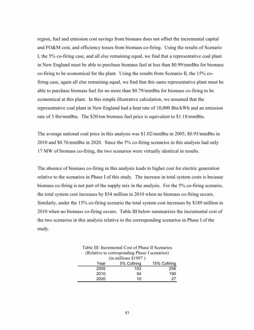
83

region, fuel and emission cost savings from biomass does not offset the incremental capital

and FO&M cost, and efficiency losses from biomass co-firing. Using the results of Scenario

I, the 5% co-firing case, and all else remaining equal, we find that a representative coal plant

in New England must be able to purchase biomass fuel at less than $0.99/mmBtu for biomass

co-firing to be economical for the plant. Using the results from Scenario II, the 15% co-

firing case, again all else remaining equal, we find that this same representative plant must be

able to purchase biomass fuel for no more than $0.79/mmBtu for biomass co-firing to be

economical at this plant. In this simple illustrative calculation, we assumed that the

representative coal plant in New England had a heat rate of 10,000 Btu/kWh and an emission

rate of 3 lbs/mmBtu. The $20/ton biomass fuel price is equivalent to $1.18/mmBtu.

The average national coal price in this analysis was $1.02/mmBtu in 2005, $0.93/mmBtu in

2010 and $0.76/mmBtu in 2020. Since the 5% co-firing scenarios in this analysis had only

17 MW of biomass co-firing, the two scenarios were virtually identical in results.

The absence of biomass co-firing in this analysis leads to higher cost for electric generation

relative to the scenarios in Phase I of this study. The increase in total system costs is because

biomass co-firing is not part of the supply mix in the analysis. For the 5% co-firing scenario,

the total system cost increases by $54 million in 2010 when no biomass co-firing occurs.

Similarly, under the 15% co-firing scenario the total system cost increases by $189 million in

2010 when no biomass co-firing occurs. Table III below summarizes the incremental cost of

the two scenarios in this analysis relative to the corresponding scenarios in Phase I of the

study.

Table III: Incremental Cost of Phase II Scenarios (Relative to corresponding Phase I scenarios)

(in millions $1997 ) Year 5% Cofiring 15% Cofiring2005 103 2582010 54 1902020 10 27

84

Conclusions No penetration of biomass occurs in either of the two scenarios in this analysis. This result is

largely because the incremental capital cost, FO&M cost, and efficiency loss from biomass

co-firing is greater than the fuel and emission cost savings from using biomass.

Please feel free to call John Leahy at 703-934-3301 or Bishal Thapa at 703-934-3904 with

any questions.

REPORT DOCUMENTATION PAGE

Form Approved OMB NO. 0704-0188

Public reporting burden for this collection of information is estimated to average 1 hour per response, including the time for reviewing instructions, searching existing data sources, gathering and maintaining the data needed, and completing and reviewing the collection of information. Send comments regarding this burden estimate or any other aspect of this collection of information, including suggestions for reducing this burden, to Washington Headquarters Services, Directorate for Information Operations and Reports, 1215 Jefferson Davis Highway, Suite 1204, Arlington, VA 22202-4302, and to the Office of Management and Budget, Paperwork Reduction Project (0704-0188), Washington, DC 20503. 1. AGENCY USE ONLY (Leave blank)

2. REPORT DATE

July 2003

3. REPORT TYPE AND DATES COVERED

Subcontract Report November 6, 2001—February 28, 2003

4. TITLE AND SUBTITLE Development Strategies for Deployment of Biomass Resources in the Production of Biomass Power

6. AUTHOR(S)

Jacob Kaminsky

5. FUNDING NUMBERS

LAR-2-31121-01

7. PERFORMING ORGANIZATION NAME(S) AND ADDRESS(ES)

Jacob Kaminsky 11108 Swansfield Rd. Columbia, MD 21044

8. PERFORMING ORGANIZATION

REPORT NUMBER

9. SPONSORING/MONITORING AGENCY NAME(S) AND ADDRESS(ES)

National Renewable Energy Laboratory 1617 Cole Blvd. Golden, CO 80401-3393

10. SPONSORING/MONITORING

AGENCY REPORT NUMBER NREL/SR-510-33524

11. SUPPLEMENTARY NOTES

NREL Technical Monitor: Lynda Wentworth 12a. DISTRIBUTION/AVAILABILITY STATEMENT

National Technical Information Service U.S. Department of Commerce 5285 Port Royal Road

Springfield, VA 22161

12b. DISTRIBUTION CODE

13. ABSTRACT (Maximum 200 words) The study analyzes strategies for deployment of biomass resources for biopower generation. It compares biomass supply databases and the projected biopower market penetration for several alternative incentive scenarios. It analyzes the availability of biomass to meet the projected market demands and recommends future research.

15. NUMBER OF PAGES

14. SUBJECT TERMS biomass resources; biomass power; biopower market demands

16. PRICE CODE

17. SECURITY CLASSIFICATION

OF REPORT Unclassified

18. SECURITY CLASSIFICATION

OF THIS PAGE Unclassified

19. SECURITY CLASSIFICATION

OF ABSTRACT Unclassified

20. LIMITATION OF ABSTRACT

UL

NSN 7540-01-280-5500 Standard Form 298 (Rev. 2-89) Prescribed by ANSI Std. Z39-18 298-102