DEVELOPMENT OF WATER QUALITY PARAMETER … · Total Suspended Solids, Chlorophyll-A, Landsat-8,...
8
DEVELOPMENT OF WATER QUALITY PARAMETER RETRIEVAL ALGORITHMS FOR ESTIMATING TOTAL SUSPENDED SOLIDS AND CHLOROPHYLL-A CONCENTRATION USING LANDSAT-8 IMAGERY AT POTERAN ISLAND WATER N. Laili a , F. Arafah a , L.M. Jaelani a *, L. Subehi e , A. Pamungkas b , E.S. Koenhardono c , A. Sulisetyono d a b Dept. of Geomatics Engineering, Faculty of Civil Engineering and Planning; Dept. of Urban and Regional Planning, Faculty of Civil Engineering and Planning; c Dept. of Marine Engineering, Faculty of Marine Technology; d Dept. of Naval Architecture and Shipbuilding Engineering, Faculty of Marine Technology, Institut Teknologi Sepuluh Nopember, Surabaya, 60111, Indonesia. Email: [email protected], [email protected], [email protected], [email protected], [email protected], [email protected] e Research Centre for Limnology, Indonesian Institute of Sciences, Cibinong Science Centre, 16911, Indonesia. Email: [email protected] KEYWORDS : Total Suspended Solids, Chlorophyll-A, Landsat-8, Poteran Island Water. ABSTRACT: The Landsat-8 satellite imagery is now highly developed compares to the former of Landsat projects. Both land and water area are possibly mapped using this satellite sensor. Considerable approaches have been made to obtain a more accurate method for extracting the information of water area from the images. It is difficult to generate an accurate water quality information from Landsat images by using some existing algorithm provided by researchers. Even though, those algorithms have been validated in some water area, but the dynamic changes and the specific characteristics of each area make it necessary to get them evaluated and validated over another water area. This paper aims to make a new algorithm by correlating the measured and estimated TSS and Chla concentration. We collected in-situ remote sensing reflectance, TSS and Chl-a concentration in 9 stations surrounding the Poteran islands as well as Landsat 8 data on the same acquisition time of April 22, 2015. The regression model for estimating TSS produced high accuracy with determination coefficient (R 2 ), NMAE and RMSE of 0.709; 9.67 % and 1.705 g/m 3 respectively. Whereas, Chla retrieval algorithm produced R 2 of 0.579; NMAE of 10.40% and RMSE of 51.946 mg/m 3 . By implementing these algorithms to Landsat 8 image, the estimated water quality parameters over Poteran island water ranged from 9.480 to 15.801 g/m 3 and 238.546 to 346.627 mg/m 3 for TSS and Chl-a respectively. 1. INTRODUCTION To support the sustainable development of water environment, a routine water quality monitoring is a critical requirement. By considering the spatial and temporal heterogeneity of water bodies, extracting water information by remote sensing techniques can be more effective approach than a direct field measurement (Liu, Islam, and Gao 2003) The estimation of water quality parameters such as the concentration of TSS (Total suspended sediments) and Chl-a (Chlorophyll-a) from satellite images is strongly depend on the accuracy of atmospheric correction and water quality parameter retrievals algorithms (Ruddick, Ovidio, and Rijkeboer 2000; Sathyendranath, Prieur, and Morel 1987; Yang et al. 2011; Jaelani et al. 2013; Jaelani, Matsushita, et al. 2015). Numerous researches have been conducted to develop and validate both atmospheric correction algorithm and water quality parameter retrieval algorithm. Since the development of first algorithm needs a comprehensive study and rigorous spectral data over study area (Jaelani, Matsushita, et al. 2015; Jaelani et al. 2013), this paper only focus on the second issue. Even though, there were many existing water quality parameter retrieval algorithms to estimate TSS and Chl-a concentration of water from satellite images (Sathyendranath and Platt 1989; Gons, Auer, and Effler 2008; Sathyendranath, Prieur, and Morel 1987; Nas et al. 2009; Dall’Olmo et al. 2005; Han and Jordan 2005; Bhatti et al. 2010; Bailey and Werdell 2006), those algorithms have been developed and validated using in situ data that was collected in some specific water area. Since, the dynamic changes and the specific characteristics of water make them unsuitable for another water area such as in Indonesia. Consequently, The objective of the present study was to develop more accurate TSS and Chl-a concentration retrieval algorithms for Landsat 8 images at Poteran island water of Indonesia using in situ spectra, TSS and Chl-a concentration. 2. METHODS To develop a new algorithm for TSS and Chl-a concentration retrieval algorithms, we collected concurrent in situ and Landsat 8 data from Poteran island water on April 22, 2015. The water area is located in Sumenep Sub-district, southeastearn Madura Island. The in situ data were measured and collected at 9 stations as shown in Fig. 1 and Table 1. For each station, we collected remote sensing reflectance (Rrs) (were measured using a FieldSpec HandHeld spectroradiometer in the range of 325–1075 nm at 1 nm intervals), and water samples that analyzed in laboratory furthermore. TSS concentration was gravimetrically extracted from water sample, whereas Chl-a concentration was analyzed using spectrophotometer at four wavelengths (750, 663, 645, and 630 nm). ISPRS Annals of the Photogrammetry, Remote Sensing and Spatial Information Sciences, Volume II-2/W2, 2015 Joint International Geoinformation Conference 2015, 28–30 October 2015, Kuala Lumpur, Malaysia This contribution has been peer-reviewed. The double-blind peer-review was conducted on the basis of the full paper. doi:10.5194/isprsannals-II-2-W2-55-2015 55
Transcript of DEVELOPMENT OF WATER QUALITY PARAMETER … · Total Suspended Solids, Chlorophyll-A, Landsat-8,...

DEVELOPMENT OF WATER QUALITY PARAMETER RETRIEVAL ALGORITHMS FOR ESTIMATING TOTAL SUSPENDED SOLIDS AND CHLOROPHYLL-A
CONCENTRATION USING LANDSAT-8 IMAGERY AT POTERAN ISLAND WATER
N. Lailia, F. Arafaha, L.M. Jaelania*, L. Subehie, A. Pamungkasb, E.S. Koenhardonoc, A. Sulisetyonod
a b Dept. of Geomatics Engineering, Faculty of Civil Engineering and Planning; Dept. of Urban and Regional Planning, Faculty of
Civil Engineering and Planning; cDept. of Marine Engineering, Faculty of Marine Technology; dDept. of Naval Architecture and
Shipbuilding Engineering, Faculty of Marine Technology, Institut Teknologi Sepuluh Nopember, Surabaya, 60111, Indonesia.
Email: [email protected], [email protected], [email protected], [email protected],
[email protected], [email protected] e Research Centre for Limnology, Indonesian Institute of Sciences, Cibinong Science Centre, 16911, Indonesia.
Email: [email protected] KEYWORDS : Total Suspended Solids, Chlorophyll-A, Landsat-8, Poteran Island Water.
ABSTRACT:
The Landsat-8 satellite imagery is now highly developed compares to the former of Landsat projects. Both land and water area are
possibly mapped using this satellite sensor. Considerable approaches have been made to obtain a more accurate method for extracting
the information of water area from the images. It is difficult to generate an accurate water quality information from Landsat images by
using some existing algorithm provided by researchers. Even though, those algorithms have been validated in some water area, but the
dynamic changes and the specific characteristics of each area make it necessary to get them evaluated and validated over another water
area. This paper aims to make a new algorithm by correlating the measured and estimated TSS and Chla concentration. We collected
in-situ remote sensing reflectance, TSS and Chl-a concentration in 9 stations surrounding the Poteran islands as well as Landsat 8 data
on the same acquisition time of April 22, 2015. The regression model for estimating TSS produced high accuracy with determination
coefficient (R2), NMAE and RMSE of 0.709; 9.67 % and 1.705 g/m3 respectively. Whereas, Chla retrieval algorithm produced R2 of
0.579; NMAE of 10.40% and RMSE of 51.946 mg/m3. By implementing these algorithms to Landsat 8 image, the estimated water
quality parameters over Poteran island water ranged from 9.480 to 15.801 g/m3 and 238.546 to
346.627 mg/m3 for TSS and Chl-a respectively.
1. INTRODUCTION
To support the sustainable development of water environment,
a routine water quality monitoring is a critical requirement. By
considering the spatial and temporal heterogeneity of water
bodies, extracting water information by remote sensing
techniques can be more effective approach than a direct field
measurement (Liu, Islam, and Gao 2003)
The estimation of water quality parameters such as the
concentration of TSS (Total suspended sediments) and Chl-a
(Chlorophyll-a) from satellite images is strongly depend on the
accuracy of atmospheric correction and water quality parameter
retrievals algorithms (Ruddick, Ovidio, and Rijkeboer 2000;
Sathyendranath, Prieur, and Morel 1987; Yang et al. 2011;
Jaelani et al. 2013; Jaelani, Matsushita, et al. 2015).
Numerous researches have been conducted to develop and
validate both atmospheric correction algorithm and water
quality parameter retrieval algorithm. Since the development of
first algorithm needs a comprehensive study and rigorous
spectral data over study area (Jaelani, Matsushita, et al. 2015;
Jaelani et al. 2013), this paper only focus on the second issue.
Even though, there were many existing water quality parameter
retrieval algorithms to estimate TSS and Chl-a concentration of
water from satellite images (Sathyendranath and Platt 1989;
Gons, Auer, and Effler 2008; Sathyendranath, Prieur, and
Morel 1987; Nas et al. 2009; Dall’Olmo et al. 2005; Han and
Jordan 2005; Bhatti et al. 2010; Bailey and Werdell 2006),
those algorithms have been developed and validated using in
situ data that was collected in some specific water area. Since,
the dynamic changes and the specific characteristics of water
make them unsuitable for another water area such as in
Indonesia.
Consequently, The objective of the present study was to develop
more accurate TSS and Chl-a concentration retrieval algorithms
for Landsat 8 images at Poteran island water of Indonesia using
in situ spectra, TSS and Chl-a concentration.
2. METHODS
To develop a new algorithm for TSS and Chl-a concentration
retrieval algorithms, we collected concurrent in situ and
Landsat 8 data from Poteran island water on April 22, 2015.
The water area is located in Sumenep Sub-district,
southeastearn Madura Island. The in situ data were measured
and collected at 9 stations as shown in Fig. 1 and Table 1. For
each station, we collected remote sensing reflectance (Rrs)
(were measured using a FieldSpec HandHeld spectroradiometer
in the range of 325–1075 nm at 1 nm intervals), and water
samples that analyzed in laboratory furthermore. TSS
concentration was gravimetrically extracted from water sample,
whereas Chl-a concentration was analyzed using
spectrophotometer at four wavelengths (750, 663, 645, and 630
nm).
ISPRS Annals of the Photogrammetry, Remote Sensing and Spatial Information Sciences, Volume II-2/W2, 2015 Joint International Geoinformation Conference 2015, 28–30 October 2015, Kuala Lumpur, Malaysia
This contribution has been peer-reviewed. The double-blind peer-review was conducted on the basis of the full paper. doi:10.5194/isprsannals-II-2-W2-55-2015
55

Water
Station
Water Quality Rrs (sr-
1)
Chl-a
(mg/m3) TSS
(g/m3)
440
nm 480
nm 560
nm 655
nm 865
nm
St.1 278 14 0.018 0.019 0.019 0.010 0.003
St.2 286 13 n/a n/a n/a n/a n/a
St.3 298 13 0.043 0.046 0.043 0.024 0.017
St.4 280 15 0.043 0.045 0.047 0.030 0.019
St.5 254 14 0.046 0.045 0.042 0.026 0.018
St.6 386 16 0.063 0.065 0.067 0.057 0.046
St.7 459 18 0.035 0.039 0.046 0.030 0.012
St.8 327 17 n/a n/a n/a n/a n/a
St.9 332 16 0.016 0.023 0.027 0.015 0.001
Table 1. Field measurements data
A regression model between every single band (band 1-5) or
band-ratio of Landsat with in situ TSS and Chl-a concentration
were assessed to find the most strongest correlation.
In addition, we collected Landsat 8 image (path/row = 117/65)
at the same time of field campaign time. This data was used to
map Chl-a and TSS concentration spatially.
Since, the Landsat-8 data (level 1T) was stored in digital
number (DN). It has to be radiometrically converted to the top-
of-atmosphere radiance (LTOA) by using following formula.
(1)
Where:
= TOA spectral radiance
= Band-specific multiplicative rescaling factor
= Digital number
= Band-specific additive scaling factor
After obtaining the radiance value, the next step was
atmospheric correction that will automatically convert the top-
of-atmosphere radiance value (LTOA) to bottom-ofatmosphere
reflectance (ρBOA). Then, the BOA Reflectance was converted
to Reflectance remote-sensing (Rrs) value.
To correct the image from atmospheric effect, we used
Second Simulation of a Satellite Signal in the Solar
Spectrum-Vector (6SV) algorithm (Vermote et al. 1997) that
calculated atmospheric-corrected reflectance for image from
three parameters as follow:
(2)
(3)
(4)
Where :
acr = Atmospherically corrected reflectance
Lλ = TOA Radiance measured data Rrs(λ) = Reflectance
remote-sensing xa, xb, xc = Atmospherical correction
parameters coefficient.
The image was now stored in Rrs(λ) value. This value was
required in order to estimate water quality parameters (TSS and
Chl-a concentration) based on the developed water quality
retrieval algorithms in previous step.
To assess the accuracy of the developed algorithms, a formula
of RMSE (Root Mean Square Error) and NMAE (Normalized
Mean Absolute Error) were used.
(5)
(6)
is the value of TSS and chlorophyll-a estimated by using
the algorithms. is the value of measured TSS and
chlorophyll-a. is the number of samples. The determination
coefficient (R2 ) was also calculated to assess the relationship
between estimated and measured concentrations.
3. RESULTS
3.1 The relationship of the measured and estimated Rrs(λ)
values
There were two data collections of the remote sensing
reflectance (Rrs(λ)) values, one was obtained from field
measurements (measured-Rrs(λ)) and the second was estimated
from the Landsat-8 image by performing radiometric
calibration and atmospheric correction (estimated- Rrs(λ)).
These data were presented in Fig. 2 and 3.
Figure 1. Field Measurements Locations at Poteran Island
ISPRS Annals of the Photogrammetry, Remote Sensing and Spatial Information Sciences, Volume II-2/W2, 2015 Joint International Geoinformation Conference 2015, 28–30 October 2015, Kuala Lumpur, Malaysia
This contribution has been peer-reviewed. The double-blind peer-review was conducted on the basis of the full paper. doi:10.5194/isprsannals-II-2-W2-55-2015
56
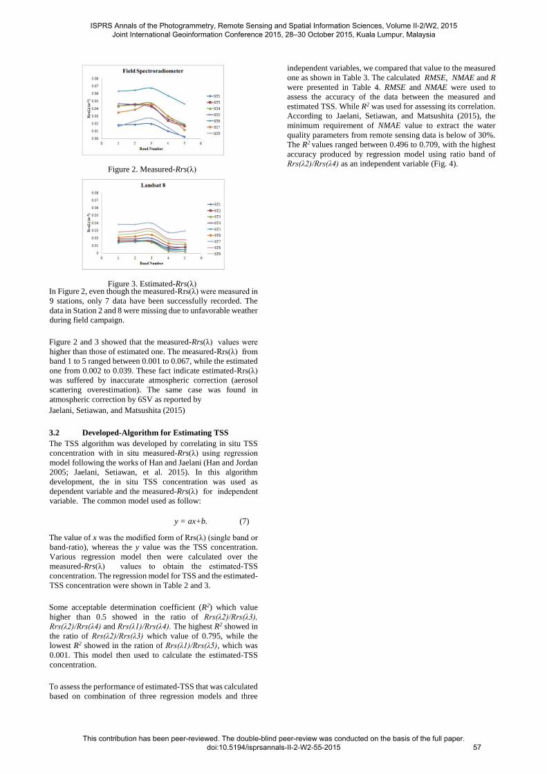
In Figure 2, even though the measured-Rrs(λ) were measured in
9 stations, only 7 data have been successfully recorded. The
data in Station 2 and 8 were missing due to unfavorable weather
during field campaign.
Figure 2 and 3 showed that the measured-Rrs(λ) values were
higher than those of estimated one. The measured-Rrs(λ) from
band 1 to 5 ranged between 0.001 to 0.067, while the estimated
one from 0.002 to 0.039. These fact indicate estimated-Rrs(λ)
was suffered by inaccurate atmospheric correction (aerosol
scattering overestimation). The same case was found in
atmospheric correction by 6SV as reported by
Jaelani, Setiawan, and Matsushita (2015)
3.2 Developed-Algorithm for Estimating TSS
The TSS algorithm was developed by correlating in situ TSS
concentration with in situ measured-Rrs(λ) using regression
model following the works of Han and Jaelani (Han and Jordan
2005; Jaelani, Setiawan, et al. 2015). In this algorithm
development, the in situ TSS concentration was used as
dependent variable and the measured-Rrs(λ) for independent
variable. The common model used as follow:
y = ax+b. (7)
The value of x was the modified form of Rrs(λ) (single band or
band-ratio), whereas the y value was the TSS concentration.
Various regression model then were calculated over the
measured-Rrs(λ) values to obtain the estimated-TSS
concentration. The regression model for TSS and the estimated-
TSS concentration were shown in Table 2 and 3.
Some acceptable determination coefficient (R2) which value
higher than 0.5 showed in the ratio of Rrs(λ2)/Rrs(λ3),
Rrs(λ2)/Rrs(λ4) and Rrs(λ1)/Rrs(λ4). The highest R2 showed in
the ratio of Rrs(λ2)/Rrs(λ3) which value of 0.795, while the
lowest R2 showed in the ration of Rrs(λ1)/Rrs(λ5), which was
0.001. This model then used to calculate the estimated-TSS
concentration.
To assess the performance of estimated-TSS that was calculated
based on combination of three regression models and three
independent variables, we compared that value to the measured
one as shown in Table 3. The calculated RMSE, NMAE and R
were presented in Table 4. RMSE and NMAE were used to
assess the accuracy of the data between the measured and
estimated TSS. While R2 was used for assessing its correlation.
According to Jaelani, Setiawan, and Matsushita (2015), the
minimum requirement of NMAE value to extract the water
quality parameters from remote sensing data is below of 30%.
The R2 values ranged between 0.496 to 0.709, with the highest
accuracy produced by regression model using ratio band of
Rrs(λ2)/Rrs(λ4) as an independent variable (Fig. 4).
Figure 2. Measured - Rrs (λ)
Figure 3. Estimated - Rrs (λ)
ISPRS Annals of the Photogrammetry, Remote Sensing and Spatial Information Sciences, Volume II-2/W2, 2015 Joint International Geoinformation Conference 2015, 28–30 October 2015, Kuala Lumpur, Malaysia
This contribution has been peer-reviewed. The double-blind peer-review was conducted on the basis of the full paper. doi:10.5194/isprsannals-II-2-W2-55-2015
57

This algorithm then be applied to the Landsat-8 image to obtain the estimated TSS values. Those estimated values with the highest R2 then be validated to the measured one as shown in Fig. 5.
Regression model Rrs(λ1) Rrs(λ2) Rrs(λ3) Rrs(λ4) Rrs(λ5)
TSS = a(xi) + b 0.001 0.003 0.075 0.107 0.006
TSS = a*log(xi) + b 0.002 0.004 0.069 0.104 0.001
Regression model Rrs(λ4)/Rrs(λ5) Rrs(λ3)/
Rrs(λ4)
Rrs(λ3)/Rrs(λ5) Rrs(λ2)/Rrs(λ3) Rrs(λ2)/Rrs(λ4)
TSS = a(xi/xj) + b 0.056 0.204 0.038 0.722 0.664
TSS = a*log(xi/xj) + b 0.072 0.192 0.025 0.733 0.628
TSS = a*(log(xi)/log(xj)) +
b
0.141 0.202 0.041 0.794 0.696
Regression model Rrs(λ2)/Rrs(λ5) Rrs(λ1)/Rrs(λ2) Rrs(λ1)/Rrs(λ3) Rrs(λ1)/Rrs(λ4) Rrs(λ1)/Rrs(λ5)
TSS = a(xi/xj) + b 0.025 0.156 0.429 0.746 0.011
TSS = a*log(xi/xj) + b 0.006 0.142 0.389 0.736 0.001
TSS = a*(log(xi)/log(xj)) +
b
0.002 0.163 0.465 0.738 0.002
Table 2. Regression model combination for TSS with R2
3 Estimated TSS (g/m )
Station Rrs(λ2)/Rrs(λ3) R=0,722 0,733 0,794
0,664
Rrs(λ2)/ Rrs(λ4) 0,628 0,696
R 0,746
rs(λ1) /
Rrs(λ4) 0,736 0,738
TSS (g/m3)
ST 1 14.80 15.22 14.67 9.25 1.79 12.53 9.85 0.90 0.48 14 ST 2 13.47 12.32 13.65 11.46 4.63 13.29 11.42 0.90 0.48 13 ST 3 13.28 11.91 13.53 -4.55 -9.51 9.48 -1.90 0.86 0.47 13 ST 4 15.45 16.70 15.26 13.83 8.45 14.46 13.68 0.92 0.48 15 ST 5 15.17 16.04 14.97 10.09 2.79 12.77 10.82 0.90 0.48 14 ST 6 15.79 17.52 15.62 14.43 9.56 14.78 14.54 0.92 0.48 16 ST 7 15.06 15.80 15.02 15.96 12.87 15.80 15.37 0.93 0.48 18 ST 8 15.87 17.71 15.79 15.36 11.48 15.36 15.12 0.93 0.48 17 ST 9 16.57 19.45 16.49 15.02 10.75 15.15 14.92 0.93 0.48 16
Measured
Table 3. The estimated-TSS for specific independent variable
Regression Model RMSE(g/m3) NMAE
(%)
R2
Rrs(λ2) Rrs(λ3)
Rrs(λ2) Rrs(λ4)
Rrs(λ1) Rrs(λ4)
Rrs(λ2) Rrs(λ3)
Rrs(λ2) Rrs(λ4)
Rrs(λ1) Rrs(λ4)
Rrs(λ2) Rrs(λ3)
Rrs(λ2) Rrs(λ4)
Rrs(λ1) Rrs(λ4)
TSS = a(xi/xj) + b 1.191 6.325 5.451 5.622 28.164 25.506 0.496 0.501 0.505 TSS = a*log(xi/xj) + b 1.817 10.646 14.295 10.627 64.724 93.915 0.488 0.681 0.679 TSS = a*(log(xi)/log(xj)) +
b 1.196 1.705 14.727 5.729 9.667 96.797 0.518 0.709 0.703
Table 4. The RMSE, NMAE and R2 as indicator of algorithm performance
ISPRS Annals of the Photogrammetry, Remote Sensing and Spatial Information Sciences, Volume II-2/W2, 2015 Joint International Geoinformation Conference 2015, 28–30 October 2015, Kuala Lumpur, Malaysia
This contribution has been peer-reviewed. The double-blind peer-review was conducted on the basis of the full paper. doi:10.5194/isprsannals-II-2-W2-55-2015
58

Figure 4.Regression model for TSS with independent
variable of band-ratio of Rrs(λ2)/Rrs(λ4)
Figure 5. Estimated vs. Measured TSS
Considering the results showed in Fig. 5, the algorithm used to
estimates the TSS values over the Landsat-8 image can now be
arranged following the formula below :
(8)
(9)
Then,
(10)
The estimated-TSS concentration from Landsat-8 images was
presented as well as the measured concentration in Table
5.
Table 5. The value of estimated and measured-TSS
ISPRS Annals of the Photogrammetry, Remote Sensing and Spatial Information Sciences, Volume II-2/W2, 2015 Joint International Geoinformation Conference 2015, 28–30 October 2015, Kuala Lumpur, Malaysia
This contribution has been peer-reviewed. The double-blind peer-review was conducted on the basis of the full paper. doi:10.5194/isprsannals-II-2-W2-55-2015
59

3.3 Developed Algorithm for Estimating Chlorophyll-a
The Chlorophyll-a estimation from spectra data follow the same step of TSS. The modeling was made using regression models with single band and band-ratio of Landsat were
Figure 6. Regression model for Chl-a with independent
variable of band-ratio of Rrs(λ2)/Rrs(λ4)
Station Estimated Chl-a
(mg/m3)
Measured Chl-a
(mg/m3 )
St.1 248.8729 278
St.2 263.228 286
St.3 238.546 298
St.4 295.538 280
St.5 252.5938 254
St.6 306.2124 386
St.7 346.6274 459
St.8 328.1409 327
presented in Table 6.
Regression model
R2
Rrs(λ1) Rrs(λ2) Rrs(λ3) Rrs(λ4) Rrs(λ5)
Chl = ax + b 0.017 0.048 0.172 0.108 0.052
Chl = ax2 – bx + c 0.036 0.059 0.182 0.199 0.111
Chl = a*log(x) + b 0.014 0.046 0.151 0.183 0.019
Chl = a*( log(x) )2 – b*log(x) + c 0.032 0.046 0.151 0.184 0.051
Regression model
R2
Rrs(λ4)/Rrs(λ5) Rrs(λ3)/ Rrs(λ4) Rrs(λ3)/ Rrs(λ5) Rrs(λ2)/Rrs(λ3) Rrs(λ2)/Rrs(λ4)
Chl = a*(xi/xj)+ b 0.002 0.231 0 0.491 0.564
Chl = a*(xi/xj)2 – b*(xi/xj) + c 0.006 0.232 0.009 0.524 0.593
Chl = a*log(xi/xj)+ b 0.005 0.231 0.001 0.500 0.576
Chl = a*( log(xi/xj))2 – b*(log(xi/xj)) + c 0.021 0.232 0.007 0.529 0.578
Chl = a*(log(xi)/log(xj))+ b 0.031 0.219 0.001 0.572 0.605
Chl = a*(log(xi)/log(xj))2 – b*(log(xi)/log(xj))+
c
0.056 0.236 0.030 0.634 0.615
Regression model
R2
Rrs(λ2)/
Rrs(λ5)
Rrs(λ1) /
Rrs(λ2)
Rrs(λ1) /
Rrs(λ3)
Rrs(λ1) /
Rrs(λ4)
Rrs(λ1) /
Rrs(λ5)
Chl = a(xi/xj) + b 0.001 0.076 0.269 0.566 0.007
Chl = a*( xi/xj)2 – b*( xi/xj ) + c 0.047 0.419 0.429 0.584 0.073
Chl = a*log(xi/xj) + b 0.009 0.060 0.224 0.573 0.023
Chl = a*( log(xi/xj))2 – b*(log(xi/xj)) + c 0.048 0.444 0.496 0.575 0.077
Chl = a*(log(xi)/log(xj)) + b 0.015 0.083 0.295 0.566 0.049
Chl = a*(log(xi)/log(xj))2 – b*(log(xi)/log(xj))+
c
0.074 0.453 0.499 0.569 0.106
Table 6. Regression model combination for Chl-a with R2
ISPRS Annals of the Photogrammetry, Remote Sensing and Spatial Information Sciences, Volume II-2/W2, 2015 Joint International Geoinformation Conference 2015, 28–30 October 2015, Kuala Lumpur, Malaysia
This contribution has been peer-reviewed. The double-blind peer-review was conducted on the basis of the full paper. doi:10.5194/isprsannals-II-2-W2-55-2015
60

St.9 319.9305
332
Table 7. The value of estimated and measured-Chl-a
Figure 7. Estimated vs. Measured Chl-a
Figure 6 showed the regression model for Chl-a concentration
estimation that was built using band-ratio of Rrs(λ2)/Rrs(λ4)
an independent variable. This model had a highest correlation
between measured-Chl and remote sensing reflectance with R2
of 0.615. The summary of developed algorithm as follow:
(11)
(12)
Therefore, the above algorithm was used to calculate the
estimated-Chl-a concentration from Landsat-8 image
reflectance. The calculation results of estimated concentration
of chlorophyll-a in 9 stations shown in Table 7 and Fig. 7.
4. CONCLUSION
We developed a new algorithm for estimating TSS and Chl-a
concentration that was applicable in small part of Indonesia
water. For that purposes, We collected in-situ remote sensing
reflectance, TSS and Chl-a concentration in 9 stations
surrounding the Poteran islands as well as Landsat 8 data on the
same acquisition time of April 22, 2015.
The regression model for estimating
TSS (
) produced high accuracy with
determination coefficient (R2), NMAE and RMSE of 0.709;
9.67%; and 1.705 g/m3 respectively. Whereas, Chl-a retrieval
algorithm
)
produced R2 of 0.579; NMAE of 10.40%; and RMSE of 51.946
mg/m3. By implementing these algorithms to Landsat 8 image,
the estimated water quality parameters over Poteran island
water ranged from 9.480 to 15.801 g/m3 and 238.546 to 346.627
mg/m3 for TSS and Chl-a respectively.
In general, the developed algorithm for estimating TSS and Chl-
a concentration produced acceptable accuracy (NMAE < 30%),
thus extracting water information from satellite images using
these algorithms are applicable. Whereas, the low correlation
between measured and estimated-Chl-a concentration
(R2=0.597) was caused not only by performance of the
developed-Chl-a estimation algorithm but also the accuracy of
atmospheric correction algorithm by 6SV.
To assess the implementation in wider area, in short future, we
are going to validate the developed algorithms using in situ data
collected in different water area in Indonesia.
ACKNOWLEDGEMENTS
This research is a part of Sustainable Island Development
Initiatives (SIDI) Program, a collaborative research in small
island development between Indonesia and Germany.
REFERENCES
Bailey, Sean W., and P. Jeremy Werdell. 2006. “A MultiSensor Approach for the on-Orbit Validation of Ocean Color Satellite Data Products.” Remote Sensing of Environment 102 (1-2): 12–23. doi:10.1016/j.rse.2006.01.015.
http://linkinghub.elsevier.com/retrieve/pii/S003442570
6000472.
Bhatti, Asif M, Donald Rundquist, John Schalles, Mark
Steele, and Masataka Takagi. 2010. “QUALITATIVE
ASSESSMENT OF INLAND AND COASTAL
WATERS BY USING.” In Remote Sensing Science, Spatial Information, XXXVIII:415–20.
Dall’Olmo, Giorgio, Anatoly A. Gitelson, Donald C.
Rundquist, Bryan Leavitt, Tadd Barrow, and John C.
Holz. 2005. “Assessing the Potential of SeaWiFS and
MODIS for Estimating Chlorophyll Concentration in
Turbid Productive Waters Using Red and near-Infrared Bands.” Remote Sensing of Environment 96 (2): 176– 87. doi:10.1016/j.rse.2005.02.007.
http://linkinghub.elsevier.com/retrieve/pii/S003442570
5000854.
Gons, Herman J., Martin T. Auer, and Steven W. Effler. 2008.
“MERIS Satellite Chlorophyll Mapping of
Oligotrophic and Eutrophic Waters in the Laurentian Great Lakes.” Remote Sensing of Environment 112 (11): 4098–4106. doi:10.1016/j.rse.2007.06.029. http://linkinghub.elsevier.com/retrieve/pii/S003442570 8002083.
Han, Luoheng, and Karen J. Jordan. 2005. “Estimating and
Mapping Chlorophyll- a Concentration in Pensacola
Bay, Florida Using Landsat ETM+ Data.”
International Journal of Remote Sensing 26 (23):
5245–54. doi:10.1080/01431160500219182.
http://www.tandfonline.com/doi/abs/10.1080/0143116
0500219182.
ISPRS Annals of the Photogrammetry, Remote Sensing and Spatial Information Sciences, Volume II-2/W2, 2015 Joint International Geoinformation Conference 2015, 28–30 October 2015, Kuala Lumpur, Malaysia
This contribution has been peer-reviewed. The double-blind peer-review was conducted on the basis of the full paper. doi:10.5194/isprsannals-II-2-W2-55-2015
61

Jaelani, Lalu Muhamad, Bunkei Matsushita, Wei Yang, and
Takehiko Fukushima. 2013. “Evaluation of Four
MERIS Atmospheric Correction Algorithms in Lake Kasumigaura, Japan.” International Journal of Remote Sensing 34 (24). Taylor & Francis: 8967–85. doi:10.1080/01431161.2013.860660. http://dx.doi.org/10.1080/01431161.2013.860660.
———. 2015. “An Improved Atmospheric Correction
Algorithm for Applying MERIS Data to Very Turbid
Inland Waters.” International Journal of Applied Earth
Observation and Geoinformation 39 (July). Elsevier
B.V.: 128–41. doi:10.1016/j.jag.2015.03.004.
http://dx.doi.org/10.1016/j.jag.2015.03.004.
Jaelani, Lalu Muhamad, Fajar Setiawan, and Bunkei
Matsushita. 2015. “Uji Akurasi Produk
ReflektanPermukaan Landsat Menggunakan Data In
Situ Di
Danau Kasumigaura , Jepang.” In Pertemuan Ilmiah Tahunan Masyarakat Penginderaan Jauh Indonesia, 9–16. Bogor: MAPIN. doi:10.13140/RG.2.1.4002.8003.
Jaelani, Lalu Muhamad, Fajar Setiawan, Hendro Wibowo, and
Apip. 2015. “Pemetaan Distribusi Spasial
Konsentrasi Klorofil-A Dengan Landsat 8 Di Danau
Matano Dan Danau Towuti , Sulawesi Selatan.” In Pertemuan Ilmiah Tahunan Masyarakat Penginderaan Jauh Indonesia, 1–8. Bogor: MAPIN. doi:10.13140/RG.2.1.1905.6484.
Liu, Yansui, Md Anisul Islam, and Jay Gao. 2003. “Quantification of Shallow Water Quality Parameters by Means of Remote Sensing.” Progress in Physical Geography 27 (1): 24–43. doi:10.1191/0309133303pp357ra.
http://ppg.sagepub.com/cgi/doi/10.1191/0309133303p
p357ra.
Nas, Bilgehan, Hakan Karabork, Semih Ekercin, and Ali Berktay. 2009. “Mapping Chlorophyll-a through inSitu Measurements and Terra ASTER Satellite Data.”
Environmental Monitoring and Assessment 157 (1-4):
375–82. doi:10.1007/s10661-008-0542-9.
http://www.ncbi.nlm.nih.gov/pubmed/18821023.
Ruddick, Kevin George, Fabrice Ovidio, and Machteld
Rijkeboer. 2000. “Atmospheric Correction of
SeaWiFS Imagery for Turbid Coastal and Inland
Waters.” Applied Optics 39 (6): 897–912.
http://www.opticsinfobase.org/abstract.cfm?URI=ao39-
6-897.
Sathyendranath, S, and T Platt. 1989. “Remote Sensing of Ocean Chlorophyll: Consequence of Nonuniform Pigment Profile.” Applied Optics 28 (3): 490–95. http://www.ncbi.nlm.nih.gov/pubmed/20548508.
Sathyendranath, S., L. Prieur, and A. Morel. 1987. “An Evaluation of the Problems of Chlorophyll Retrieval
from Ocean Colour, for Case 2 Waters.” Advances in Space Research 7 (2): 27–30. doi:10.1016/02731177(87)90160-8. http://linkinghub.elsevier.com/retrieve/pii/0273117787 901608.
Vermote, E.F., D. Tanre, J.L. Deuze, M. Herman, and J.-J.
Morcette. 1997. “Second Simulation of the Satellite
Signal in the Solar Spectrum, 6S: An Overview.” IEEE Transactions on Geoscience and Remote Sensing 35 (3): 675–86. doi:10.1109/36.581987.
http://ieeexplore.ieee.org/lpdocs/epic03/wrapper.htm?a
rnumber=581987.
Yang, Wei, Bunkei Matsushita, Jin Chen, and Takehiko
Fukushima. 2011. “Estimating Constituent
Concentrations in Case II Waters from MERIS Satellite Data by Semi-Analytical Model Optimizing and Look-up Tables.” Remote Sensing of Environment 115 (5). Elsevier Inc.: 1247–59. doi:10.1016/j.rse.2011.01.007.
http://linkinghub.elsevier.com/retrieve/pii/S003442571
1000204.
ISPRS Annals of the Photogrammetry, Remote Sensing and Spatial Information Sciences, Volume II-2/W2, 2015 Joint International Geoinformation Conference 2015, 28–30 October 2015, Kuala Lumpur, Malaysia
This contribution has been peer-reviewed. The double-blind peer-review was conducted on the basis of the full paper. doi:10.5194/isprsannals-II-2-W2-55-2015
62