Development of Two-Phase Flow Correlation in Boiling Water

13

Development of Two-Phase Flow Correlation for Fluid Mixing Phenomena

in Boiling Water Reactor

Hiroyuki Yoshida and Kazuyuki Takase Japan Atomic Energy Agency

Japan

1. Introduction

The two-phase fluid mixing phenomena in fuel bundles of BWR plays an important role in the thermal-hydraulic performance of the fuel rod bundle, because it has strong effects on spatial distributions of the void fraction, quality and mass flow rate within it. The subchannel analysis method has been used for the prediction of the macroscopic thermal-hydraulic characteristics, such as critical power and pressure loss, of a wide variety of fuel rod bundle designs. This method evaluates the fluid mixing effects using a unique model, known as a “cross flow model”. The first successful cross flow model for gas-liquid two-phase flow was devised by Lahey and Moody (1993). In their model, cross flow phenomena were decomposed into three components, namely flow diversions caused by transverse pressure gradients, turbulent mixing caused by stochastic pressure and flow fluctuations and a void drift that is unique to gas-liquid two-phase flow. Recently, there were studies of cross flow model improvements. Kawahara et al. (1999)

presented an improved turbulent mixing model based on RMS (Root Mean Square) values

of subchannel-to-subchannel differential pressure fluctuations. One of the advantages of this

model was its ability to consider channel gap geometries and scales. Sumida et al.(1995) and

Takemoto et al.(1997) supposed that the turbulent mixing and void drift phenomena were

only transient components of the diversion cross flow caused by differential pressure

fluctuations between the subchannels, and formulated the model known as the “fluctuating

pressure model”. Although both models appear promising for predicting the fluid mixing

phenomena however, their applicability under actual plant operation conditions is presently

unclear because it is impossible to simulate differential pressure fluctuations under steam-

water high-pressure conditions without relying on experimental data. Although the cross

flow model remains the most popular approach today, the mechanics of the third

component, the void drift, are still unclear and there is no widely accepted understanding of

it yet.

In the cross flow model and subchannel analysis, two-phase flow correlations are used to evaluate effects of flow conditions on two-phase flow characteristic easily. To create, modify or confirm these correlations, “actual scale tests” those simulate flow conditions and flow channel of actual fuel bundles are required. In actual BWR, pressure and temperature equals to about 7.2MPa and 560K respectively. Then the actual scale tests take a long time and

www.intechopen.com

Computational Simulations and Applications

288

entail great cost, development of a method that enables the thermal-hydraulic design of BWRs without these actual size tests is desired. It is expected that large scale numerical simulations (numerical simulations by large scale computer) would replace certain large-scale tests and thermal-hydraulic information, some of which is currently difficult or impossible to measure experimentally, would be obtained. And new design method will be developed based on these numerical simulations. For this reason we developed an advanced thermal-hydraulic design method for BWRs using innovative two-phase flow simulation technology. For this, the following are required: (1) an advanced simulation method with high accuracy prediction, (2) verification of simulation method; and, (3) analytical method to confirm or modify the correlations by detailed numerical simulation data. In this study, we are developing the method to create or modify the two-phase flow correlations for the fluid mixing phenomena in BWR based on advanced numerical simulation technic.

2. Numerical simulation method

The fluid mixing phenomena dominates water and steam distribution in the fuel bundles

and is one of the most important phenomena that affect boiling transition (BT) of BWRs.

Surface tension at gas-liquid interface (interface), shapes of interfaces and pressure

difference fluctuation between subchannels play important roles in these phenomena. Then

an advanced simulation method developed in this study must evaluate surface tension,

interface shape and pressure fluctuation accurately. To satisfy these requirements, we

developed an advanced simulation code: TPFIT and an advanced interface tracking method.

Detail of the TPFIT and the advanced interface tracking method are explained in this

section.

2.1 Governing equation and numerical simulation To calculate surface tension and interface shapes by realistic computational resources, the

TPFIT adopt interface tracking method. In two-phase flow in rod bundles, compressibility of

steam has important influence for pressure difference fluctuation between subchannels. In

TPFIT, considering the time-dependent Navier-Stokes equation for two phase compressible

flow, conservative equations of mass of liquid, mass of gas, momentum and energy are

described as follows:

Mass of liquid:

0kl l

k

f u f

t x

(1)

Mass of gas:

0kg g

k

f u f

t x

(2)

Momentum:

1i i ik

k i i

k i k

pu uu g

t x x x

(3)

www.intechopen.com

Development of Two-Phase Flow Correlation for Fluid Mixing Phenomena in Boiling Water Reactor

289

Energy:

1k

k

k k k k

upe e Tu q

t x x x x

(4)

where u, p, e, T are velocity, static pressure, internal energy and temperature, and g and in the momentum equation are gravity and surface tension force, respectively. In above equations, subscripts g and l are used to represent gas and liquid phases. The mass of liquid and gas phases in two phase flow are defined as following equation.

l ll

g gg

f f

f f

(5)

In Eq. (5), f is volume fraction of fluid, and Volume fraction of gas phase is evaluated by use of volume fraction of liquid.

g l

f = 1 - f (6)

Two-phase fluid density is calculated as sum of mass of both phases:

l g

f f (7)

Eqs. (1) and (2) are solved in the advanced interface tracking method described in sec.2.2. The momentum equation (Eq. (3)) is solved by the CIP (Cubic Interpolated Pseudo-particle) method (Yabe and Aoki, 1991). The energy equation (Eq. (4)) is used to obtain the Poison equation for static pressure. Temperature is estimated by means of a fluid property routine based on the static pressure and local density of both phases. The ILUCGS method is used to solve the Poison equation for static pressure. In the TPFIT code, a Cartesian coordinate system and staggered grid are used. The surface tension force in the momentum equation is estimated using the CSF model (Blackbill et al., 1992). In the CSF model, volume fraction of liquid fl is required and evaluated in the advanced interface tracking method, too. The local viscosities and thermal conductivities of liquid and gas were evaluated using solved static pressure and temperature fields based on the fluid property routine.

2.2 Outline of advanced interface tracking method The fundamental concept of the advanced interface tracking method is quite simple. That is, a transported volume of liquid and gas between neighboring calculation control volumes during each time step is calculated through the movement of approximated gas-liquid interfaces, as estimated in the Lagrangian system. Schematic drawings of the major three operational steps within each time step in the two-dimensional case are shown in Figure 1. In the first step (reconstruction step), as shown in Figure 1 (a), a gas-liquid interface in each control area for calculations is reconstructed, taking account of the liquid fraction represented by it and its surroundings. In the reconstruction step, the gas-liquid interface is approximated by a linear function: F(x) as same as PLIC (Gueyffier, et al., 1999) method (see Fig.2 for 3-dimensional case). The function F(x) is expressed as follows:

1

1 2 3, , ,mn

i i

i

F a x b x x x

x x (8)

www.intechopen.com


290

In the equation, nm represents dimension of simulation, and is 2 or 3. xi is the coordinate position of the definition point of scalar quantities. A unit normal vector to the interface a= (a1,a2,a3) and segment b in Eq.(8) must be estimated. To evaluate the function f(x), we assumed that the interface exists in the position where volume fraction of liquid fl equals to 0.5. By least-squares method (choose eight nearest neighbors for 2-dimensional case, 26 nearest neighbors for 3-dimensional case), linear function is obtained.

1

00.5mn

i i

i

lF f a x b

x (9)

In the equation, b0 is segment of linear function evaluated by least square method. Control volume is divided into two polyhedrons by the linear functions. If gray polyhedron in Fig.2 corresponds to liquid region in control volume, volume of this polyhedron: Vl must be equals to proper volume of liquid. Thus,

l l

V f V (10)

where V is a volume of computational cell given by following equation for 3-dimensional cases.

1 2 3· ·V x x x (11)

To satisfy Eq. (10), the segment b is adjusted as fraction Vl/V agrees with volumetric fraction of fluid. Between the volume of fluid Vl and segment b, there is the relation that is expressed as the following equation for three dimensional cases.

3 33 33

1 11 2 3

1max , 0 max , 0

6m i i m i i

i i

V b b a x b b a xa a a

(12)

In this equation, bm is the maximum value that b can take:

3

1

m i i

i

b a x

. (13)

In this study, the Newton's method is used to estimate the segment b that satisfies Eq. (12). In the next step (transportation step), polyhedrons within each control volume are transported along a surrounding velocity field (Fig.1 (b)). Some parts of the volume of this polyhedron are transported to surrounding control volume. For example, in Fig.1(b), V is transferred from control volume 1 to control volume 2. Each transferred volume of liquid is calculated in this step. And each transferred volume of gas is also calculated by a procedure same as the volume of liquid.

Fig. 1. (a) Reconstruction step

www.intechopen.com


291

Liquid

Gas

u t

Control volume 1 (CV1)

Control volume 2 (CV2)

Transported volume V from CV1 to CV2

(b) Transportation step

V

olu

me

frac

tion

(c) Redistribution step

Fig. 1. Schematic drawings of volume fraction transport calculation using the advanced interface tracking method (2-dimensional case).

In transportation step, transfer volume of both phases is calculated. In the last step (redistribution step), as shown in Fig.1(c), transferred mass of both phases can be evaluated by multiplying density by transferred volume. Mass at new time step can be calculated by summing these transferred mass.

x2

x1

x3

x2

x 3

x 1

-b/a1

-b/a2

-b/a3

3

1

0i

iibxa

Fig. 2. Approximated fluid segment in control volume (3-dimensional case).

www.intechopen.com


292

3. Validation of TPFIT for fluid mixing phenomena

We try to validate the TPFIT with the advanced interface tracking method developed in this study for fluid mixing phenomena.

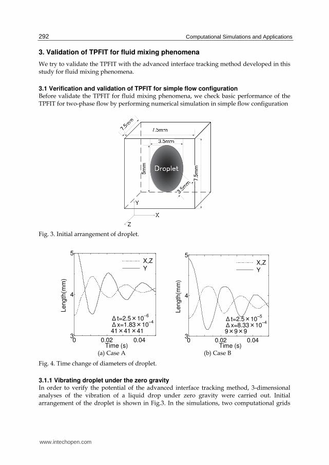
3.1 Verification and validation of TPFIT for simple flow configuration Before validate the TPFIT for fluid mixing phenomena, we check basic performance of the TPFIT for two-phase flow by performing numerical simulation in simple flow configuration

7.5mm

5mm

Fig. 3. Initial arrangement of droplet.

0 0.02 0.043

4

5

Time (s)

Len

gth

(mm

)

X,Z

Y

Δt=2.5×10–6

Δx=1.83×10–4

41×41×41

0 0.02 0.04

3

4

5

Time (s)

Length

(mm

)

X,Z

Y

Δt=2.5×10–5

Δx=8.33×10–4

9×9×9

(a) Case A (b) Case B

Fig. 4. Time change of diameters of droplet.

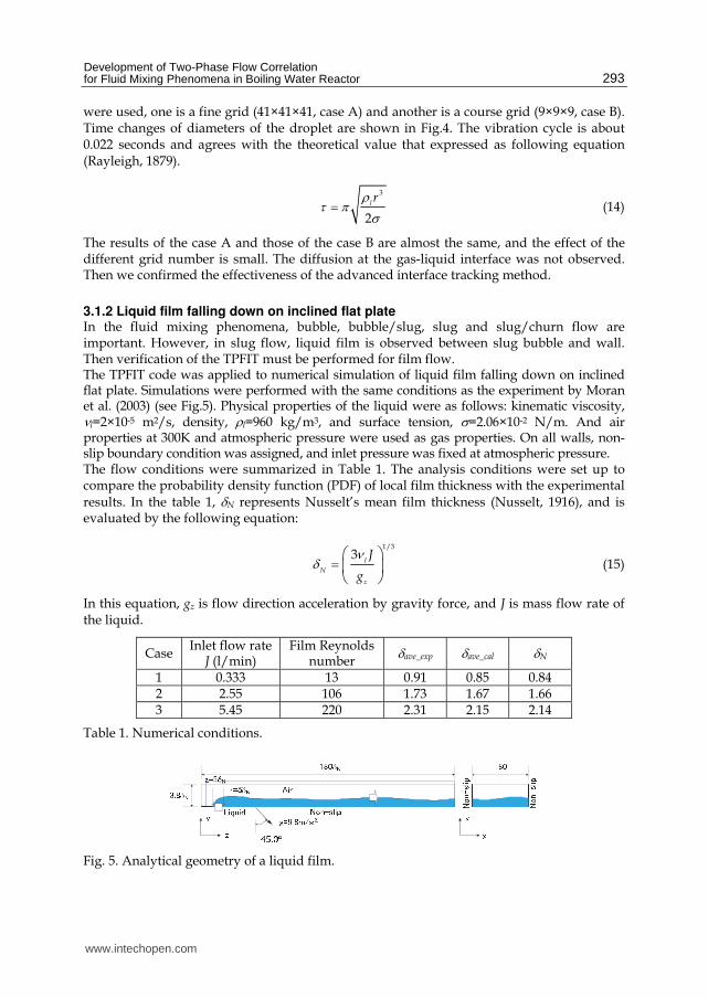
3.1.1 Vibrating droplet under the zero gravity In order to verify the potential of the advanced interface tracking method, 3-dimensional analyses of the vibration of a liquid drop under zero gravity were carried out. Initial arrangement of the droplet is shown in Fig.3. In the simulations, two computational grids

www.intechopen.com


293

were used, one is a fine grid (41×41×41, case A) and another is a course grid (9×9×9, case B). Time changes of diameters of the droplet are shown in Fig.4. The vibration cycle is about 0.022 seconds and agrees with the theoretical value that expressed as following equation (Rayleigh, 1879).

3

2

lr (14)

The results of the case A and those of the case B are almost the same, and the effect of the different grid number is small. The diffusion at the gas-liquid interface was not observed. Then we confirmed the effectiveness of the advanced interface tracking method.

3.1.2 Liquid film falling down on inclined flat plate In the fluid mixing phenomena, bubble, bubble/slug, slug and slug/churn flow are important. However, in slug flow, liquid film is observed between slug bubble and wall. Then verification of the TPFIT must be performed for film flow. The TPFIT code was applied to numerical simulation of liquid film falling down on inclined flat plate. Simulations were performed with the same conditions as the experiment by Moran et al. (2003) (see Fig.5). Physical properties of the liquid were as follows: kinematic viscosity, l=2×10-5 m2/s, density, l=960 kg/m3, and surface tension, =2.06×10-2 N/m. And air properties at 300K and atmospheric pressure were used as gas properties. On all walls, non-slip boundary condition was assigned, and inlet pressure was fixed at atmospheric pressure. The flow conditions were summarized in Table 1. The analysis conditions were set up to compare the probability density function (PDF) of local film thickness with the experimental results. In the table 1, N represents Nusselt’s mean film thickness (Nusselt, 1916), and is evaluated by the following equation:

1/3

3l

N

z

J

g

(15)

In this equation, gz is flow direction acceleration by gravity force, and J is mass flow rate of the liquid.

Case Inlet flow rate

J (l/min)Film Reynolds

numberave_exp ave_cal N

1 0.333 13 0.91 0.85 0.84 2 2.55 106 1.73 1.67 1.66 3 5.45 220 2.31 2.15 2.14

Table 1. Numerical conditions.

Fig. 5. Analytical geometry of a liquid film.

www.intechopen.com


294

(a) t=0.00s (b) t=0.02s

(c) t=0.04s (d) t=0.08s

(e) t=0.2s (f) t=0.4s

Fig. 6. Observed liquid film shapes.

Figure 6 shows snapshot of the numerical results of the Case 3. In this study, the calculated gas-liquid interfaces were defined as isosurface at a volume fraction of liquid of 0.5. In 0.02s, two-dimensional wave was observed near liquid inlet section, and this wave moves to the downstream section. From 0.04 seconds later, small three-dimensional waves occurred on the surface of the liquid film. After that, these small waves gradually becomes big until t=0.2s. At t=0.4s, the liquid film exhibited a smooth, flat gas-liquid interface upon immediate entrance to the test section, but after a short distance small, small ripples were observed at

the interface. At approximately 200mm (about z=100 N) from the inlet, the small ripples developed into a three-dimensional structure characterized by large waves, and wave structures were almost developed at this point. In general, the degree of waviness increased with increasing film Reynolds number. The average local film thicknesses in the numerical

result (ave_cal) at x=20mm and z=175 N are shown in Table 1 and almost agreed with

Nusselt’s mean film thickness. However, ave_cal were slightly smaller than the average film

thickness in the experimental results (ave_exp).

The probability density functions (PDF) of liquid film thickness at x=20mm and z=175 N

were evaluated to compare numerical results with the experimental results quantitatively.

Figure 7 shows the PDF of film thickness. At low Reynolds numbers (Ref=13), the PDF

distributions showed a sharp peak (first peak) at about average film thickness, but remained

www.intechopen.com


295

close to zero for greater thickness values, indicating existence of few waves. At low film

Reynolds number, the position and height of the first peak agreed well in the analysis and

experiment.

(a) Case 1 (b) Case 2 (c) Case 3

Fig. 7. Probability density function of liquid film thickness.

In the experimental results, at relatively high Reynolds number (Ref=106 and 220),

additional smaller peaks (second peaks) appeared to the right of the main peaks. Because

the sampling numbers (ns) used in the processing of the experimental data (ns = 60) were

smaller than those in the numerical results (ns =1200), scattered results were observed in the

experimental PDF distributions. As shown in Fig.8, the numerical result agreed well with

the experimental result including existence of second peaks and these positions. The

predicted values of minimum liquid film thickness by the numerical simulations were

slightly smaller than those measured by the experiments without relying on the mass flow

rate of the liquid. It is thought that because the predicted minimum liquid film thicknesses

were thin, the average liquid film thicknesses became smaller in comparison with the

experimental results.

3.1.3 Bubbly and slug flow in square duct By two-phase correlations for fluid mixing phenomena, volume or mass cross flow rate or

mixing coefficients are evaluated. Then volume and mass conservation of two-phase flow is

important function. As mentioned above, volume conservation equations for both phases

are not solved, and the TPFIT has no special treatment to keep volume conservation. Then

we must check volume conservation of the TPFIT. In two-phase flow fluid mixing

phenomena, the maximum value of mixing gas flow rate is around 10% of gas flow rate in

flow channel. An error of the volume conservation must be done below 1% if we want to

predict mixing coefficient with accuracy of less than 10%.

Case Fluid Inlet Inlet void fraction: in Inlet velocity: win

1 Air-water at 0.1MPa and 300K

A 0.307

0.5 m/s 2 B 0.111

3 Steam-water at 7.2MPa and 560K

A 0.307

4 B 0.111

Table 2. Numerical condition for bubbly flow in square duct.

www.intechopen.com


296

To check volume conservation, the TPFIT was applied to bubbly and slug flow in square duct. Numerical domain is shown in Fig.8 (a), and numerical conditions are shown in table 2. In the simulations, air-water and steam-water two-phase flow were used. Air-water two-phase flow at atmospheric pressure is used as working fluid in many experimental researches, and the TPFIT was applied to these experiments for validation. Then we used in this simulation. Steam-water two-phase flow at 7.2MPa and 560K (saturation temperature at 7.2MPa) is appeared in real (actual) reactor conditions. Two-phase flow correlations will be checked or examined at this conditions, we also used in this simulation. On all walls, non-slip boundary condition was assigned, and inlet velocity and volume fraction of liquid were fixed. Outlet pressure was also fixed at atmospheric pressure or 7.2MPa.

14.00

14.00

14.00

4.67

x

z

x

y

x

y

Inlet A

Inlet B

Case 1 Case 2

(a) Numerical Domain (b) Example of Interface shape

Fig. 8. Numerical domain and example of interface shape.

Figure.8 (b) shows example of interface shapes. Different two-phase flows were formed in a square duct by the difference in inlet volume fraction. And complicated interface shapes were observed in higher volume fraction case (Case 1). Figure 9 shows evaluated volume conservation error. In this figure, Evol was volume conservation error and defined as following equation.

,

1g

vol

g in

VolE

Vol , (16)

where Volg is calculated total gas volume in a square duct by use of simulated results. And Volg,in is total gas volume calculated by use of inlet condition of simulations:

,

· · ·g in i inn

V wo tl A , (17)

where, A is area of square duct (=14×14=196mm2), t is time. In Case 1 and 2, differences between gas density and liquid density was relatively large, and effects of compressibility of

www.intechopen.com


297

gas was also large. Then, large fluctuation of Evol in Case 1 and 2 was observed. However, except these fluctuations, the maximum value of volume conservation error: Evol were less than 0.2%. Therefore, it was confirmed that the TPFIT has enough performance of volume conservation to simulate two-phase flow fluid mixing phenomena.

0 0.05 0.1−0.005

0

0.005

t [s]

EV

ol[−]

Case 1Case 2Case 3Case 4

Fig. 9. Evaluated volume conservation error for two-phase flow in square duct.

3.2 Verification for fluid mixing phenomena by experimental data

In the next step, we must validate TPFIT for fluid mixing phenomena. To evaluate TPFIT

performance for two-phase flow fluid mixing phenomena between the subchannels,

numerical simulations for two-phase flow fluid mixing tests were performed.

3.2.1 Air-water fluid mixing test

TPFIT code was applied to 2-channel air-water mixing tests (Yoshida, 2007). The dimension

of calculated test channel is shown in Fig.10 (a). The test channel, which consists of two

parallel subchannels with an 8×8 mm square cross section and the interconnection, is 220

mm long and air and water flow upwards in it. The interconnection’s gap clearance,

horizontal and vertical length are 1.0 mm, 5.0 mm and 20 mm respectively. An irregular

mesh division in the Cartesian system was adopted and two subchannels and the

interconnection were formed by using obstacles as shown in Fig.11. The total number of

effective control volumes was 428,680 respectively. The fluid mixing was observed at

interconnection in the experiments. A non-slip wall, constant exit pressure and constant

inlet velocity were selected as boundary conditions for each subchannel. The time step was

controlled with a typical safety factor of 0.2 to keep it lower than the limitation value given

by the Courant condition and stability condition of the CSF model. Calculation conditions

are shown in Table 3.

www.intechopen.com


298

Fig. 10. Calculated test channel.

Fig. 11. Calculation meshes in channel cross section for air-water fluid mixing test.

Water inlet velocity (m/s) Injected air volume (cc)

Ch.1 Ch.2 Ch.1 Ch.2

0.26 0.26 1.27 1.50

Table 3. Air-water flow calculation condition.

The slug behavior observed around the interconnection is shown in Fig.12 (a). Once the top

of an ascending air slug in Ch.1 reaches the center height of the interconnection, part of it

starts to be drawn toward Ch. 2. Then the tip of stretched part of the air slug flows into Ch.2

through the interconnection and is separated to form a single bubble. The calculated air slug

behavior is shown in Fig.12 (b). As shown in Fig.12 (b), any intrusion of air into the

interconnection as well as any separation of the air slug can be effectively calculated. The

www.intechopen.com


299

moved bubble volumes from Ch.1 to Ch.2 were estimated to be 0.087cc in the observation

and 0.094cc in the calculation.

Fig. 12. Observed and calculated slug behavior of air-water fluid mixing test around the interconnection.

3.2.2 Steam-water fluid mixing under high pressure The TPFIT was applied to steam water fluid mixing test (Yoshida, 2007). Calculated test channels used in these simulations are shown in Fig.10 (b). The calculation conditions are shown in Table 4. An irregular mesh division in the Cartesian system was adopted and two subchannels and the interconnection were formed by using obstacles as shown in Fig.13. The total number of effective control volumes was 2,647,400 respectively. A non-slip wall, constant exit pressure, and constant inlet velocity were selected as boundary conditions for each subchannel.

Fig. 13. Calculation meshes in channel cross section for steam-water fluid mixing test.

www.intechopen.com


300

Inlet mass flow rate (kg/s) Inlet quality (%)

Ch.1 Ch.2 Ch.1 Ch.2

0.44 0.23 0.0 0.47

Table 4. Steam-water flow calculation condition.

Fig. 14. Observed and calculated slug behavior of steam-water fluid mixing test around the interconnection.

The slug behaviors observed and calculated around the interconnection is shown in Fig.14. As shown in Fig.14 (a), a part of single steam slug in Ch.2 intrudes to the Ch.1 through the interconnection. Averaged slug length is about 56 mm, and observed major slug characteristic behavior is as follows.

Steam intrusion from Ch.2 to Ch.1 is firstly occurred at the upper part of the steam slug (“A” in the Fig.14).

Constriction is generated at the center part of the steam slug by water flow from Ch1 to Ch.2, and the steam slug break up (“B” in the Fig.14).

As shown in Fig.14 (b), the occurrence of intrusion of steam from the Ch.2 to the Ch.1 can be effectively calculated, and the calculated amount of steam penetration into the interconnection looks quite similar to the observed one. Predicted slug length is about 59 mm, and almost same as the observed one. As shown in Fig.14 (b), the major slug characteristic behavior observed in the experiment was reproduced in the numerical simulation by TPFIT code. The measured and calculated differential pressure and cross flow rate between Ch.1 and Ch.2 for steam-water flow are shown in Figs.15 and 16 respectively. The calculated values of the differential pressure and the cross flow rate agreed well with the measured values.

www.intechopen.com


301

Fig. 15. Measured and calculated pressure difference between subchannels.

○Measured

● Predicted


3.2.3 Numerical simulation of air-water two-phase flow in modeled 2 subchannels The TPFIT code was applied to experimental analyses of the existing 2-channel fluid mixing experiments (Sumida, 1995), and comparisons between measured and calculated results were carried. In the experiments, the differential pressure between the subchannel at the center height of the mixing section and the exit air and water flow rate of each subchannel were measured. Numerical analyses of air-water flow fluid mixing were applied between the length of -100mm and +60mm from the lower edge of the mixing section in the flow direction of the test channel as shown in Fig.17 (a). The flow area is divided into two channels by a flat plate (partition plate). At the upper part of the partition plate, there was a narrow slit, through which the channels were connected. The flow channel was divided into 3 parts, developing section, mixing section and outlet section. The narrow slit was located in the mixing section, and fluid mixing was occurred at this section. The developing section was set up to get developed flow at inlet of the mixing section. The outlet section was located at top of the calculated test channel to let out air-water two-phase flow smoothly.

www.intechopen.com


302

Air

Slit

Mixingsection

Developingsection

Outletsection

50

10

100

z

x

Air

Slit

Mixingsection

Developingsection

Outletsection

50

10

100

z

x

Channel 1

Channel 2

(a) Calculated test channel (b) Calculation mesh

Fig. 17. Dimensions of calculated test channel and calculation meshes in channel cross section for air-water two-phase flow.

Regular mesh division in the Cartesian system was adopted and two subchannels and the

interconnection were formed by using obstacles as shown in Fig.17 (b). The calculation mesh

size was set to 2/3 mm to satisfy the condition that the number of the calculation meshes of

gap region must be more than 6, and the total number of the calculation meshes was

496,800. A non-slip wall, constant exit pressure and constant inlet velocity were selected as

boundary conditions for each subchannel. The effects of the contact angle of the water on

the channel walls were set to 15 degree.

Case Inlet liquid mass flux (kg/m2s) Inlet quality (%)

Ch.1 Ch.2 Ch.1 Ch.2

L1

370 0.0013

0.0007

L2 0.0013

L3 0.0019

L4 0.0026

H1

277 0.0022

0.0011

H2 0.0022

H3 0.0033

H4 0.0044

Table 5. Air-water flow calculation condition.

Air and water were injected through the air and water inlet section located at lower part of the modeled test channel (see Fig.17 (a)). The area of the air and water inlet section was

www.intechopen.com


303

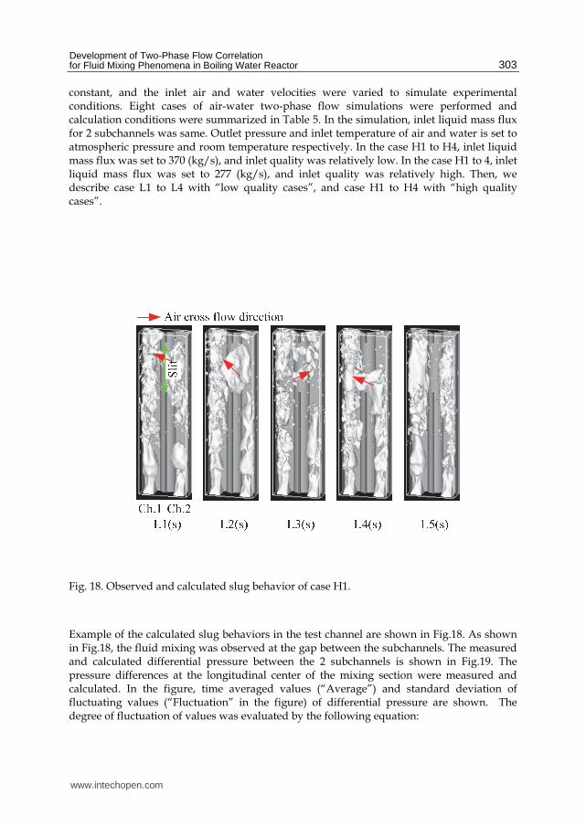
constant, and the inlet air and water velocities were varied to simulate experimental conditions. Eight cases of air-water two-phase flow simulations were performed and calculation conditions were summarized in Table 5. In the simulation, inlet liquid mass flux for 2 subchannels was same. Outlet pressure and inlet temperature of air and water is set to atmospheric pressure and room temperature respectively. In the case H1 to H4, inlet liquid mass flux was set to 370 (kg/s), and inlet quality was relatively low. In the case H1 to 4, inlet liquid mass flux was set to 277 (kg/s), and inlet quality was relatively high. Then, we describe case L1 to L4 with “low quality cases”, and case H1 to H4 with “high quality cases”.

Fig. 18. Observed and calculated slug behavior of case H1.

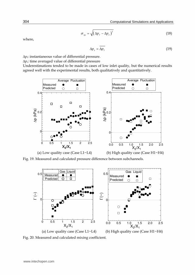
Example of the calculated slug behaviors in the test channel are shown in Fig.18. As shown in Fig.18, the fluid mixing was observed at the gap between the subchannels. The measured and calculated differential pressure between the 2 subchannels is shown in Fig.19. The pressure differences at the longitudinal center of the mixing section were measured and calculated. In the figure, time averaged values (“Average”) and standard deviation of fluctuating values (“Fluctuation” in the figure) of differential pressure are shown. The degree of fluctuation of values was evaluated by the following equation:

www.intechopen.com


304

2

p T Sp p (18)

where,

S T

p p (19)

pt: instantaneous value of differential pressure.

ps: time averaged value of differential pressure Underestimations tended to be made in cases of low inlet quality, but the numerical results agreed well with the experimental results, both qualitatively and quantitatively.

0

Measured

FluctuationAverage

Predicted

0 0.5 1 1.5 2 2.5

0

0.2

0.4

X2/X1

p (k

Pa)

X2/X1

0.0 0.5 1.0 1.5 2.0 2.5

0

0.2

0.4

Measured

FluctuationAverage

Predicted

X2/X1

p (k

Pa)

(a) Low quality case (Case L1~L4) (b) High quality case (Case H1~H4)


0 0.5 1 1.5 2 2.5

0

0.5

X2/X1

(–)

Gas LiquidMeasured

Predicted

0.0 0.5 1.0 1.5 2.0 2.5

0

0.5Measured

LiquidGas

Predicted

X2/X1

(−)

(a) Low quality case (Case L1~L4) (b) High quality case (Case H1~H4)

Fig. 20. Measured and calculated mixing coefficient.

www.intechopen.com


305

The measured and calculated mixing coefficients of both phases for air-water cases are shown in Fig.20. The mixing coefficients of gas and liquid are defined as below (Sumida, 1995):

1 2

m

m

m m

w

W W (20)

where, Wm1: Inlet mass flow rate of m phase for channel 1 Wm2: Inlet mass flow rate of m phase for channel 2 wm: Moved mass flow rate from channel 1 to channel 2 Underestimations tended to be made in cases of low inlet quality, but the numerical results

agreed well the experimental results. These underestimations of mixing coefficients

corresponded to those of differential pressure. It seems that a main cause of

underestimations was overestimation of the flow resistance in the gap region due to

insufficient spatial resolution when gas velocity is relatively low.

4. Development of two-phase flow correlation for fluid mixing phenomena

4.1 Evaluation of existing correlations for fluid mixing phenomena Innovative water reactor for flexible fuel cycle (FLWR) is one of new generation light water reactor and has been developed at Japan Atomic Energy Agency (Uchikawa, 2007). In order to achieve a conversion ratio higher than unity, a hexagonal tight-lattice rod bundle with about 1mm of gap width was adopted. Due to narrower rod gaps and the channels being surrounded by rods, bubble/slug-to-bubble/slug and bubble/slug-to-wall interactions may occur more frequently within the FLWRs core than in those of current BWRs, and these may affect the two-fluid mixing characteristics by way of the deformation, separation and coalescence of bubbles/slugs caused by the interactions.

4.1.1 Analytical conditions In this section, to evaluate the existing two-phase flow correlation for fluid mixing

phenomena, two-phase flow in 2 modeled subchannels for BWRs and FLWRs fuel bundles

were performed (“BWR cases” and “FLWR cases”). For this, 16 cases of two-phase flow

simulations were performed (see table 6 and 7).

Case Inlet liquid mass flux (kg/m2s) Inlet quality (%)

Ch.1 Ch.2 Ch.1 Ch.2

B1

1400

0.0067

0.0264 B2 0.0134

B3 0.0264

B4 0.0513

B5 0.0184

0.0362 B6 0.0362

B7 0.0533

B8 0.0699

Table 6. Calculation conditions for fluid mixing phenomena in BWRs fuel bundle.

www.intechopen.com


306

Steam

Slit

Mixingsection

Developingsection

200

350

z

x

Steam

Slit

Mixingsection

Developingsection

200

350

z

x

Channel 1

Channel 2

(a) Calculated test channel (b) Calculation mesh

Fig. 21. Dimensions of calculated test channel and calculation meshes for BWR cases.

The calculated test channel is shown in Fig.21 (a) and Fig.22 (a). The flow area is divided into two channels by a flat plate (partition plate) as same as the air-water cases. The flow channel is divided into 2 parts, developing section and mixing section. Liquid phase velocity in the BWR cases and the FLWR cases is relatively higher than that in air-water cases. To remove the effects on flow development and fluid mixing, length of the developing section and the mixing section were extended and the outlet section was removed.

Case Gap

width (mm)

Inlet liquid mass flux (kg/m2s) Inlet quality (%)

Ch.1 Ch.2 Ch.1 Ch.2

F1

1.3 600

150

0.05

0.21

F2

600

0.002

F3 0.03

F4 0.08

F5

1.0 600 600 0.05

0.05

F6 0.03

F7 0.08

F8 0.12

Table 7. Calculation conditions for fluid mixing phenomena in FLWRs fuel bundle.

Regular mesh division in the Cartesian system was adopted except for lower part of the developing section. In the lower part of developing section (z=0~350 mm for BWR cases, z=0~200 mm for FLWR cases), to save computational resources, a relatively coarse

computational meshes were used (z=2mm). The other region, z equals to 1mm. Two subchannels and the interconnection were formed by using obstacles. The calculation mesh

www.intechopen.com


307

size was set to 2/3 mm for BWR cases and 0.21mm or 0.16mm for FLWR cases to satisfy the condition that the number of the calculation meshes of gap region must be more than 6. A non-slip wall, constant exit pressure and constant inlet velocity were selected as boundary conditions for each subchannel.

(a) Calculated test channel

Fig. 22. Dimensions of calculated test channel and calculation meshes for FLWR cases.

To simulate the operating conditions of the BWR and the FLWR, outlet pressure and inlet temperature of steam and water is set to 7 MPa and saturation temperature at 7 MPa respectively. Steam and water were injected through the steam and water inlet section located at lower part of the modeled test channel. The steam and water inlet sections were optimized to get a developed flow at inlet of test section, and divided into twelve small sections for BWR cases.

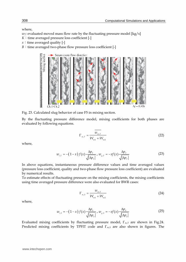
4.1.2 Evaluation of existing correlations Example of the calculated behaviors in the test channel and detail of slug behavior of are shown in Fig.23. As shown in Fig.23, the fluid mixing between Ch.1 and Ch.2 was observed at a gap between the subchannels. Though inlet quality of both subchannels were equivalent in this case (inlet quality ratio (X2/X1) was equal to 1.0), fluid mixing occurred between 2 subchannels. The existing two-phase flow correlation for fluid mixing (fluctuating pressure model (Takemoto, 1997) was evaluated using detailed numerical simulation data. The fluctuating pressure model is expressed as follows:

2

2( )

1 1 1

l T

T T

l

g

pw f x p

K x Bx

(21)

www.intechopen.com


308

where, wT: evaluated moved mass flow rate by the fluctuating pressure model [kg/s] K：time averaged pressure loss coefficient [-]

x：time averaged quality [-]

B：time averaged two-phase flow pressure loss coefficient [-]

Fig. 23. Calculated slug behavior of case F5 in mixing section.

By the fluctuating pressure difference model, mixing coefficients for both phases are evaluated by following equations.

,

,

1 2

m T

m T

m m

w

W W (22)

where,

, ,1 ( ) ( ),T T

l T g T

T T

p pw x f x w xf x

p p

(23)

In above equations, instantaneous pressure difference values and time averaged values (pressure loss coefficient, quality and two-phase flow pressure loss coefficient) are evaluated by numerical results. To estimate effects of fluctuating pressure on the mixing coefficients, the mixing coefficients using time averaged pressure difference were also evaluated for BWR cases:

,

,

1 2

m S

m S

m m

w

W W (24)

where,

, ,1 ( ) ( ),S S

l S g S

S S

p pw x f x w xf x

p p

(25)

Evaluated mixing coefficients by fluctuating pressure model, m,T are shown in Fig.24.

Predicted mixing coefficients by TPFIT code and m,S are also shown in figures. The

www.intechopen.com


309

evaluated mixing coefficients, m,T were in reasonable agreement with the predicted results.

Evaluated mixing coefficients by use of time averaged pressure difference, m,S overestimated the predicted results in almost all cases, and it is understood that the fluctuating component of pressure difference restrains the fluid mixing between subchannels.

0 1 2 3 4 5

−0.1

0

0.1

0.2

Predicted

X2/X1

g (−

)

g,Tg,S

0 1 2 3 4 5

−0.1

0

0.1

0.2

Predicted

X2/X1

l (−)

l,Tl,S

(a) Gas (b) Liquid

Fig. 24. Evaluation of the fluctuating pressure model for BWR cases (Case B1~B8).

-0.002

0.000

0.002

0.004

0.006

0.008

0.010

0.00 0.05 0.10 0.15 0.20 0.25X2(-)

Mas

s F

low

Rat

e b

etw

een

Sub

chan

nel

s (k

g/s

)

TPFITFluctuating Pressure ModelCross Flow Model

Gap Width:1.3mm

-0.0015

-0.0010

-0.0005

0.0000

0.0005

0.0010

0.0015

0.00 0.02 0.04 0.06 0.08 0.10 0.12 0.14X2(-)

Mas

s F

low

Rat

e bet

wee

n

Subch

annel

s (k

g/s

)

TPFITFluctuating Pressure ModelCross Flow Model

Gap Width:1.0mm

(a) 1.3mm gap spacing (Case F1~F4) (b) 1.0mm gap spacing (Case F5~F8)

Fig. 25. Evaluation of the existing correlations for FLWR cases (Case F1~F8).

Evaluated mixing coefficients by fluctuating pressure model and conventional fluid mixing

model (Kelly and Kazimi, 1980) for FLWR cases are shown in Fig.25. Predicted mixing

coefficients by the TPFIT are also shown in figures. The evaluated mixing coefficients by

fluctuating pressure model for relatively low inlet quality cases were in reasonable

agreement with the predicted results for both 1.3 mm and 1.0 mm gap spacing. However,

evaluated mixing coefficients by conventional fluid mixing model were different from

predicted mixing coefficients by the TPFIT code both qualitatively and quantitatively.

Evaluated mixing coefficients for relatively high inlet quality cases (inlet quality ratio

(X2/X1) is large) by fluctuating pressure model and conventional fluid mixing model

showed underestimation and overestimation respectively.

www.intechopen.com


310

4.2 Development of correlation base on detailed numerical simulation results In section 4.1, existing correlations for the two-phase flow fluid mixing phenomena were examined. However, enough results were not obtained. Then, we try to develop new correlation for fluid mixing phenomena in tight lattice rod bundle based on numerical results.

Ø13

1.30

6

Fuel rod

Fig. 26. Simulated region in rod bundle.

6

13

Developing section

Mixing section

Outlet section

Partition plate

Steam inflow section

Ch.1

Ch.2

A’

A

x= y=0.05

Water

x

y

unit:mm

z

Fig. 27. Modeled two sub-channels.

The simulated region in a tight-lattice rod bundle is schematically shown in Fig.26. The diameter of fuel rods is 13.0mm. The smallest gap spacing between two adjacent fuel rods is 1.3mm. Numerical domain used in this simulation is shown in Fig.27. The length and width of the simulated region are 13.0mm and 6.0mm respectively. The two subchannels are separated by a partition plate with the thickness of 0.2mm, in the upper part of which there is a slit with the height of 40mm. Water and steam flow into the subchannels through the

www.intechopen.com


311

bottom. Gas and liquid flows pass through three sections along the axial direction, i.e. developing, mixing and outlet sections. Grid numbers are 120×260×1600 (49,920,000). Saturated water and steam at 7.2MPa are used as working fluids. Steam and liquid are injected at constant velocities with values tabulated. The total mass flux is set to 400kg/m2s.

Fig. 28. Examples of simulation results.

Fig. 29. Axial cross-sectional averaged pressure and void fraction distribution.

www.intechopen.com


312

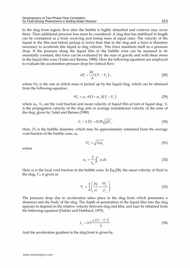
Figure 28 shows the time change of void fraction distribution observed from the section A-A’, as indicated in Fig.27. The red color denotes the fuel rod. It can be seen that the gas phases cross the slit mutually. Figure 29 shows the axial cross-sectional pressure and void distributions around a slug bubble. It illustrates that most of pressure gradient takes place in liquid slug zone and the pressure almost keeps constant in large bubble zone. Below the bubble, there exists large pressure gradient. This is reasonable because flow after the bubble is highly disturbed and vortexes may occur there. In simulation results, strong correlation for liquid phase means that liquid fluid mixing occurs due to local inter-subchannel differential pressure. Then we decided to develop an approximate model for prediction of differential pressure between subchannels. Pressure difference between subchannels is induced by difference of axial pressure distribution in each subchannel. Therefore, to evaluate mixing flow rate between subchannels by fluid mixing phenomena, axial pressure distribution in subchannels must be required. In following section, axial pressure distribution (axial pressure loss) model is developed.

Fig. 30. Physical model for slug flow.

Based on the above-mentioned results of the numerical simulation, we considered pressure distributions in bubble zone, slug front and slug core (see Fig.30). In the bubble zone, the pressure almost keeps constant in this zone. Therefore, pressure drop across a bubble zone is assumed to be zero as follows:

0bdP

dz (26)

In slug front and slug core, there are three contributions to the pressure drop across a slug. The first, dPa,s, is the pressure drop that results from the acceleration of the slow moving liquid film to slug velocity in the slug front zone. The second, dPf,s, is the pressure drop required to overcome wall shear. The third, dPg,s, is the static head pressure drop. The total pressure gradient across a liquid slug is thus given by

, ,, f s g sa ss

dP dPdPdP

dz dz dz dz . (27)

www.intechopen.com


313

In the slug front region, flow after the bubble is highly disturbed and vortexes may occur there. Then additional pressure loss must be considered. A slug that has stabilized in length can be considered as a body receiving and losing mass at equal rates. The velocity of the liquid in the film just before pickup is lower than that in the slug and a force is therefore necessary to accelerate this liquid to slug velocity. This force manifests itself as a pressure drop. If the pressure along the liquid film in the bubble zone can be assumed to be essentially constant, this force can be evaluated by the sum of gravity and wall shear stress in the liquid film zone (Taitel and Barnea, 1990). Here the following equations are employed to evaluate the acceleration pressure drop for vertical flow:

le

a s le

WP V V

A , (28)

where Wle is the rate at which mass is picked up by the liquid slug, which can be obtained from the following equation:

· · 1 ·le lle l le

W A V V (29)

where le, Vle are the void fraction and mean velocity of liquid film at font of liquid slug. Vt is the propagation velocity of the slug unit or average translational velocity of the nose of the slug, given by Taitel and Barnea (1990)

1.2 0.35l s b

V V gD (30)

Here, Db is the bubble diameter, which may be approximately estimated from the average void fraction of the bubble zone, b.

·b b

D A (31)

where

0

1 bL

b l

b

dxL

(32)

Here l is the local void fraction in the bubble zone. In Eq.(28), the mean velocity of fluid in the slug, Vs, is given as

1 gl

s

l g

WWV

A (33)

The pressure drop due to acceleration takes place in the slug front which penetrates a distances into the body of the slug. The depth of penetration of the liquid film into the slug appears to depend on the relative velocity between slug and film, and may be obtained from the following equation (Dukler and Hubbard, 1975).

2

32

·0.l s ls

sf

V VL

(34)

And the acceleration gradient in the slug front is given by,

www.intechopen.com


314

,a s a

sf

dP P

dz L

. (35)

In the slug front and slug core region, frictional and gravity pressure drop are acting in subchannels. Frictional pressure drop takes place when liquid slug moves along the channel wall. For the calculation of this term, the similarity analysis for two-phase frictional pressure drop (Dukler et al., 1975) is applied. Within the liquid slug the bubble size is usually small and thus the flow can be deemed as the homogeneous one with negligible two-phase slip. Under this condition, the frictional pressure drop can be calculated as follows:

, 221 ·

f s s

l ss g s

h

dP f

dV

z D (36)

For “non-slip” conditions fs could be correlated as a unique function of Res

0.0250.07 ·9ss

Rf e (37)

Here the Reynolds number Res is defined in the following manner:

1

1

l s g s

s h s

l s g s

Re D V

(38)

The static head term for the slug front and slug core can be obtained from the following simple equation:

,·1

g s

l s g sg

dP

dz (39)

The axial relative pressure in question could be obtained through the integration of differential pressure as follows

0

in slug zone

in bubble zone

z

s

b

dPP dz

dz

dP

dP dz

dPdz

dz

(40)

The above equations are incomplete and some parameters are still unknown, such as local void fraction in the bubble zone l, the mean velocity of liquid film at front of liquid slug, the bubble length Lb as well as that of slug unit Lu, and instantaneous bubble distribution. These parameters may be predicted by assuming the idealized bubble shape and setting the initial bubble distribution along the channel. We leave them for future study. In this study we aim at exploring the mechanism of differential pressure fluctuation inducing cross flow as a first step, therefore numerical simulation results are used to evaluate these unknown parameters for simplicity. In addition, a criterion to reduce the detailed three-dimensional simulation results is introduced to determine locations and lengths of bubble zones (or slug zones). The regions, where the cross-sectional averaged void fraction is larger than 0.3, are deemed as bubble zones. Other regions are regarded as slug zones.

www.intechopen.com


315

Fig. 31. Instantaneous axial pressure distribution.

Here, the model is evaluated with the axial pressure profile obtained from the numerical simulation for a subchannel with cross flow. Figure 31 shows the evaluation results at an instant with time of 0.8600 s. From the figure, it can be seen that the prediction of the model is generally in agreement with the simulation results, especially for mixing section (abscissa from 20 mm to 60 mm). This means the model may be applicable to subchannels. And furthermore, we can see that the three contributions to pressure drop have almost similar weights in the total pressure drop.

z=127.5mm(Distance from Outlet=32.5mm)

Fig. 32. Fluctuation of differential pressure between two subchannels.

www.intechopen.com


316

In this study, the way to evaluate the cross-section averaged pressure distribution in a single subchannel has been developed. If we assume that cross flow has minor effect on the pressure distribution in each subchannel, we can evaluate the pressure differences between subchannels by axial pressure distribution for each subchannel. In this way, the prediction of differential pressure by the model is compared to that obtained from the numerical simulation as shown in Fig. 32. It can be seen that the prediction of this model may reproduce the results of numerical simulation generally. For the time of 0.22 or 0.27, cross flow may have not negligible effect on inter-subchannel differential pressures and thus predictions deviate from the simulation results.

5. Conclusion

To perform thermal hydraulic design of the boiling water reactor (BWR) without actual

size tests, we have been developed a new design method for BWRs. In this design

method, the two-phase flow correlations for fluid mixing phenomena must be modified or

created based on results of large scale numerical simulations. Then, we developed an

innovative two-phase flow simulation code TPFIT and an advanced interface tracking

method. In the advanced interface tracking method, gas and liquid mass conservation

equations are solved, to treat compressibility of gas and to keep high volume conservation

of gas and liquid.

In the second step, to verify and validate the TPFIT with the advanced interface tracking

method, the TPFIT was applied to some experimental analyses including three the 2-channel

fluid mixing tests, and comparisons between measured and predicted result were carried

out. By these results, it was concluded that the TPFIT can be applied to the two-phase flow

fluid mixing phenomena.

In the next step, the TPFIT was applied to the numerical simulation of fluid mixing between

subchannels on a current BWR and FLWR that is one of innovative water reactor concept

developed in JAEA. The existing two-phase flow correlation for fluid mixing was evaluated

using detailed numerical simulation data. When inlet quality ratio of subchannels is

relatively large, evaluated mixing coefficients by existing two-phase flow correlations for

fluid mixing were different from those of the detailed numerical simulation data. And new

correlation based on large scale numerical simulation results are expected. In the fourth step, we tried to develop new two-phase flow correlations related to the fluid mixing phenomena. Differential pressure fluctuation between subchannels dominates the fluid mixing phenomena. We considered that the differential pressure fluctuation is induced by difference of axial pressure distribution in each subchannel. Then we developed new correlation for axial pressure distribution. In this correlation, a hydrostatic gradient, acceleration and frictional gradients are taken into account in the liquid slug, and no pressure gradient exists in the slug bubble. New correlation was validated by numerical results of the TPFIT, and it was concluded that predicted results of this correlation almost agree with the simulation results. Furthermore, differential pressure fluctuation based on predicted axial pressure distribution in subchannels can predict differential pressure by the TPFIT. We thought that the method to create new two-phase flow correlations by results of large scale numerical simulations is effective. However, there is issue such as required computational resources or validation of prediction accuracy of created correlations.

www.intechopen.com


317

6. Acknowledgment

This research was conducted using a supercomputer of the Japan Atomic Energy Agency.

7. References

Lahey, Jr, R. T. & Moody, F. J., (1993), The Thermal-Hydraulics of a Boiling Water Nuclear

Reactor, American Nuclear Society, La Grange Park, Illinois USA.

Kawahara, A., Sadatomi, M. & Tomino, T., (2000), Prediction of Gas and Liquid Turbulent

Mixing Rates between Rod Bundle Subchannels in a Two-Phase Slug-Churn Flow,

Trans. JSME, Ser. B, 66, pp. 1191-1197

Sumida, I,, Yamakita, T., Sakai, S., Iwai, K., & Kondo, T., (1995), Investigation of Two-Phase

Flow Mixing between Two Subchannels (1st Report, Fluctuating Pressure Model

and its Experimental Verification), Trans. JSME, Ser. B, 61, pp. 2662-2668 (in

Japanese).

Takemoto, S., Kondo, T., Inatomi, T., Sakai, S., Wakai, K., & Sumida, I., (1997), Investigation

of Two-Phase Flow Mixing between Two Subchannels (2nd Report, Verification of

Fluctuating Pressure Model without Steady Pressure), Trans. JSME, Ser. B, 61, pp.

3107-3113 (in Japanese).

Yabe, T., & Aoki, T., (1991), A Universal Solver for Hyperbolic Equations by Cubic-

Polynomial Interpolation I. One-Dimensional Solver, Comput.Phys.Commun., 66, pp.

219-232.

Brackbill, J. U., Kothe, D. B., & Zemach, C., (1992), A Continuum Method for Modeling

Surface Tension, J. Comput. Phys., 100, pp. 335-354.

Gueyffier, D., Nadim, J. Li, A., Scardovelli, R., & Zaleski, S., (1999), Volume-of-Fluid

Interface Tracking with Smoothed Surface Stress Methods for Three-Dimensional

Flows, J. Comput. Phys., 152, pp. 423-456.

Rayleigh, L., (1879), On the Capillary Phenomena of Jets, Proc. R. Soc. London, 29, p. 71-

97.

Moran, K., Inumaru, J., & Kawaji, M., (2002), Instantaneous hydrodynamics of a laminar

wavy liquid film, Int. J of Multiphase Flow, 28 pp.731-755.

Nusselt, W., (1916), Die oberflachenkondensation des wasserdamphes, VDI-Zs 60,

541.

Yoshida, H., Nagayoshi, T., Takase, K., & Akimoto, H., (2007), Development of Design

Technology on Thermal-Hydraulic Performance in Tight-Lattice Rod Bundles: IV -

Numerical Evaluation of Fluid Mixing Phenomena using Advanced Interface-

Tracking Method –, Proc. of ICONE15 (CD-ROM), Nagoya, Japan, September 22-26,

10532.

Uchikawa, S., Okubo, T., Kugo, T., Akie, H., Takeda, R., Nakano, Y., Ohnuki, A., &

Iwamura, T., (2007), Conceptual Design of Innovative Water Reactor for Flexible

Fuel Cycle (FLWR) and its Recycle Characteristics, J. Nucl. Sci. Tech., 44, 3, pp.277-

284.

Taitel, Y., & Barnea, D., (1990), Two-Phase Slug Flow, Advances in Heat Transfer, 20, pp. 83-

132

www.intechopen.com


318

Dukler, A. E., & Hubbard, M. G., (1975), A model for gas-liquid slug flow in horizontal and

near horizontal tubes, Ind. Eng. Chem., Fundam., 14, pp. 337-347.

Kelly, J.E., & Kazimi, M.S., (1980), Development of the two-fluid multidimensional code

THERMIT for LWR analysis, AIChE Symposium Series, pp. 149-162.

www.intechopen.com

Computational Simulations and ApplicationsEdited by Dr. Jianping Zhu

ISBN 978-953-307-430-6Hard cover, 560 pagesPublisher InTechPublished online 26, October, 2011Published in print edition October, 2011

InTech EuropeUniversity Campus STeP Ri Slavka Krautzeka 83/A 51000 Rijeka, Croatia Phone: +385 (51) 770 447 Fax: +385 (51) 686 166www.intechopen.com

InTech ChinaUnit 405, Office Block, Hotel Equatorial Shanghai No.65, Yan An Road (West), Shanghai, 200040, China

Phone: +86-21-62489820 Fax: +86-21-62489821

The purpose of this book is to introduce researchers and graduate students to a broad range of applications ofcomputational simulations, with a particular emphasis on those involving computational fluid dynamics (CFD)simulations. The book is divided into three parts: Part I covers some basic research topics and development innumerical algorithms for CFD simulations, including Reynolds stress transport modeling, central differenceschemes for convection-diffusion equations, and flow simulations involving simple geometries such as a flatplate or a vertical channel. Part II covers a variety of important applications in which CFD simulations play acrucial role, including combustion process and automobile engine design, fluid heat exchange, airbornecontaminant dispersion over buildings and atmospheric flow around a re-entry capsule, gas-solid two phaseflow in long pipes, free surface flow around a ship hull, and hydrodynamic analysis of electrochemical cells.Part III covers applications of non-CFD based computational simulations, including atmospheric opticalcommunications, climate system simulations, porous media flow, combustion, solidification, and sound fieldsimulations for optimal acoustic effects.

How to referenceIn order to correctly reference this scholarly work, feel free to copy and paste the following:

Hiroyuki Yoshida and Kazuyuki Takase (2011). Development of Two-Phase Flow Correlation for Fluid MixingPhenomena in Boiling Water Reactor, Computational Simulations and Applications, Dr. Jianping Zhu (Ed.),ISBN: 978-953-307-430-6, InTech, Available from: http://www.intechopen.com/books/computational-simulations-and-applications/development-of-two-phase-flow-correlation-for-fluid-mixing-phenomena-in-boiling-water-reactor

© 2011 The Author(s). Licensee IntechOpen. This is an open access articledistributed under the terms of the Creative Commons Attribution 3.0License, which permits unrestricted use, distribution, and reproduction inany medium, provided the original work is properly cited.

http://creativecommons.org/licenses/by/3.0

Development of Two-Phase Flow Correlation in Boiling Water

Documents

Transcript of Development of Two-Phase Flow Correlation in Boiling Water