Development of Software Sensors for Determining Total Phosphorus and Total Nitrogen in Waters

Int. J. Environ. Res. Public Health 2013, 10, 219-236; doi:10.3390/ijerph10010219

International Journal of

Environmental Research and

Public Health ISSN 1660-4601

www.mdpi.com/journal/ijerph

Article

Development of Software Sensors for Determining Total

Phosphorus and Total Nitrogen in Waters

Eunhyoung Lee 1, Sanghoon Han

1 and Hyunook Kim

2,*

1 M-Cubic Co., Ltd. Migun Technoworld, 533 Yongsan-dong, Yuseong-gu, Daejeon, 305-500,

Korea; E-Mails: [email protected] (E.L.); [email protected] (S.H.) 2 Department of Environmental Engineering, University of Seoul, 90 Jeonnong-dong,

Dongdaemun-gu, Seoul 130-743, Korea

* Author to whom correspondence should be addressed; E-Mail: [email protected];

Tel.: +82-2-2210-5408; Fax: +82-2-2210-2917.

Received: 27 November 2012; in revised form: 25 December 2012 / Accepted: 5 January 2013 /

Published: 10 January 2013

Abstract: Total nitrogen (TN) and total phosphorus (TP) concentrations are important

parameters to assess the quality of water bodies and are used as criteria to regulate the

water quality of the effluent from a wastewater treatment plant (WWTP) in Korea.

Therefore, continuous monitoring of TN and TP using in situ instruments is conducted

nationwide in Korea. However, most in situ instruments in the market are expensive and

require a time-consuming sample pretreatment step, which hinders the widespread use of

in situ TN and TP monitoring. In this study, therefore, software sensors based on

multiple-regression with a few easily in situ measurable water quality parameters were

applied to estimate the TN and TP concentrations in a stream, a lake, combined sewer

overflows (CSOs), and WWTP effluent. In general, the developed software sensors

predicted TN and TP concentrations of the WWTP effluent and CSOs reasonably well.

However, they showed relatively lower predictability for TN and TP concentrations of

stream and lake waters, possibly because the water quality of stream and lake waters is

more variable than that of WWTP effluent or CSOs.

Keywords: software sensor; total nitrogen; total phosphorus; multiple linear regression

OPEN ACCESS

Int. J. Environ. Res. Public Health 2013, 10 220

1. Introduction

The Korean Ministry of Environment has recently imposed stricter permit requirement on the

outflow of domestic wastewater treatment plants (WWTPs) to improve the water quality of receiving

water bodies such as rivers and lakes. Therefore, the water quality monitoring program has become an

important social issue.

At present, there are a total of 61 in situ monitoring stations along the banks of major streams and

lakes to measure the status of the water quality on-site. In addition, since 2008, a total of 653 tele-metering

systems have been installed at the discharge point of each of medium to large size WWTP for

monitoring effluent water quality continuously. The water quality parameters monitored by the

systems include pH, dissolved oxygen (DO), electrical conductivity (EC), turbidity (Turb), chemical

oxygen demand (COD), total nitrogen (TN), and total phosphorus (TP). Among these parameters,

TN and TP are the most important ones and obligatory parameters, and are monitored using automated

laboratory instruments, which are as expensive as 100,000 USD each. Moreover, these instruments

require time-consuming sample pretreatment before water TN and TP are determined (usually more

than 1 h), which hinders the widespread use of in situ monitoring of TN and TP.

A software sensor is a common name for the software in which a given set of water quality data

obtainable by easy and reliable methods are processed to estimate the quantities of other water quality

variables using a model [1,2]. In general, a variable that cannot be easily measurable is selected as the

one estimated by the software sensor. It is normally developed in a form of statistical models such as a

multiple linear regression (MLR) model.

The basic concept of the software sensor is illustrated in Figure 1. Measurement values for water

quality parameters that can be relatively easily measurable are fed into a software sensor (called an

estimator) and are processed to provide other water quality parameters, for examples, TN or TP [3,4].

Using software sensors, it is possible to create continuous time series of TP and TN data that can be

utilized for better understanding the timing and magnitude of TP and TN fluxes to streams or lakes.

Figure 1. Concept of software sensor.

In fact, the software sensor concept has been applied in a few studies. Christensen et al. [5,6] developed

MLR based software sensors to predict total suspended solids (TSS), fecal coliforms, and nutrients for

several streams in Kansas, USA, using real-time measured Turb, specific conductance, water temperature,

and discharge. Data from the software sensor was applied to calculate total maximum loads of the TSS

on the streams. Uhrich et al. [7] derived power regression equations for estimating suspended-sediment

concentrations from instream real-time Turb-monitor data in the upper North Santian river basin,

Oregon, USA. Zhu et al. [8] also applied an MLR-based software sensor for the prediction of stream

flow and runoff in Pennsylvania, USA, using geographic information system.


The software sensor concept also has been applied in WWTPs. Alastair et al. [9] estimated

bicarbonate alkalinity using a MLR model based on pH, redox and conductivity data to control

actuators in the anaerobic digestion process. In a study carried out by Alcaraz-González et al. [10],

flow rate, CO2 exhaust flow rate, fatty acid concentration and total inorganic carbon were utilized to

estimate microbial concentrations, alkalinity and COD in each unit processes of a WWTP. Lastly,

Feitkenhauer and Meyer [11] estimated substrate and biomass concentrations and controlled aerobic

cycle of aerobic and anoxic activated sludge process using a titrimetric technique based software sensor.

Total nitrogen and TP in streams or wastewater have been measured using software sensors by a

few researchers. Jeong et al. [12] tried to measure TN and TP in wastewater in situ using UV

absorbance and an artificial neural network (ANN)-based model. da Costa et al. [13] used an ANN

model to predict TN and PO43−

concentrations of streams. In their study, however, the ANN model was

fed with data from in situ surrogate sensors, i.e., temperature, pH, DO, and EC sensors. Ryberg [14]

and Christensen et al. [15] applied MLR models fed with data from in situ stream flow, EC, pH,

temperature, Turb, and DO sensors for predicting TN and TP of streams. Even with the data from

surrogate sensors, their models could reasonably predict the TN and TP of their streams; R2s of the

MLR models for TN and TP were 0.70, and 0.77, respectively.

In this study, software sensors (or regression models) were developed to estimate TN and TP of

different waters (i.e., streams, lakes, WWTP effluents, and CSOs) by performing MLR with water

quality parameters including pH, EC, DO, Turb, NO2–N, NO3–N, NH4–N, and PO4–P. This study was

intended to evaluate the feasibility of the software sensor concept in indirect measurement of TN and

TP in waters. Moreover, in this study, ionic nutrient species data were also included in the MLR

models, so a better model performance was expected.

2. Materials and Methods

2.1. Study Area and Data Acquisition

Water samples for the current study were collected from the Daejeon area in the middle of

South Korea (Figure 2). Water samples were collected from a total of 22 points; 15 points for stream

water samples, three for lake water, three for CSOs, and one for WWTP effluent. The predictability of

a software sensor may be improved if water qualities are measured at other points in a WWTP.

However, the water quality of only the outflow from a WWTP is under surveillance in Korea.

Therefore, in this study, we just focused on the outflow site only. The WWTP is treating domestic

wastewater and is consisted of a conventional activated sludge process and a subsequent coagulation

process for phosphorus removal. The stream under study is flowing along the urban area and receiving

treated wastewater from the WWTP. Finally, the lake is located in the upstream of the agricultural and

forestry area. The lake water samples were collected from about 0.5 m depth from the surface.

Water samples were collected weekly from March, 2011 to June, 2012. In Tables 1 and 2,

the number of water samples collected for each water type and the water quality parameters analyzed

in the laboratory are summarized, respectively. For the study, the whole observation data were divided

into two sets; one for calibration (or training) and the other for validation.


Figure 2. Water sampling locations.

( : WWTP effluent; : CSOs; : Stream; : Lake)

Namely, water quality data collected from March 2011 to August 2011 were used for model

development, and the data from September 2011 to June 2012 were used for model validation.

Table 1. Conditions of water quality analysis.

Water Type Sampling points Number of samples

WWTP effluent

CSOs

Streams

Lakes

1

3

15

3

77

239

228

1,183

All the water quality parameters except TP and TN in Table 2 were used as independent variables in

the MLR analysis: input data for a software sensor (or a regression model). The manually measured

TN and TP concentrations were compared with the ones predicted by the developed software sensors.

DO, pH, EC, and Turb were measured using a sensor (YSI6600EDS SONDE, YSI Inc., Yellow Springs,

OH, USA), while NO2–N, NO3–N, NH4–N, and PO4–P were done with ion chromatography (IC;

DIONEX-ICS-1100, Thermo-Fisher Inc., Seoul, Korea).

China

Korea

Japan

2 mi

2 km


Table 2. Water quality parameters monitored in this study.

Water quality

Parameters Unit

Measurement

Method

Variables

measured

by sensors

DO

pH

EC

Turb

mg·L−1

-

μS·cm−1

NTU

Electrode Method

(YSI6600EDS SONDE)

Variables

measured

by chemical

analysis

PO4–P

NO2–N

NO3–N

NH4–N

mg·L−1

mg·L−1

mg·L−1

mg·L−1

IC

(DIONEX-ICS-1100)

TP

TN

mg·L−1

mg·L−1

Ascorbic Acid Method

Persulfate Method

2.2. Data Processing

2.2.1. Scatter Diagram Analysis

Initially, the correlation between different water quality parameters was analyzed. For better

understanding the relationship, a scatter diagram was first drawn for pairs between TN or TP and each

of the other water quality parameters. A scatter diagram can visually show the relative strength of the

relationship between each pair of variables; the direction (i.e., positively or negatively correlated) and

shape (i.e., linear or non-linear) of the correlation can be shown. The scatter diagram shows to what

extent each water quality parameter correlates with TN and TP. The correlation coefficient between

two variables is defined as the covariance of the two variables divided by the product of their standard

deviations. Out of the scatter diagram analysis, dominant or important parameters can be derived from

all the variables; if any parameter is highly correlated with TN or TP, it can be regarded as an

important parameter.

2.2.2. Multiple Linear Regression Analysis

Dominant variables, which were derived as the result of a scatter diagram analysis, were utilized to

develop a software sensor to predict TN and TP through the MLR analysis as a next step. An MLR is

an analytical method used to develop an equation to relate a dependent variable y and one or more

independent variables. In fact, an MLR is still used extensively in practical applications. A linear

regression model or equation depends on the linear relation between its known and unknown variables,

and it is easier to fit than a non-linear model. It is also easier to determine the statistical properties of

the resulting estimators (i.e., software sensors or linear models).

A general MLR equation (or the software sensor in this study) is provided below (Equation (1)):

(1) iippiii xxxy 2211


where yi is a dependent variable (TN or TP concentration in this study), 𝑥i represents independent

variables (water quality parameters other than TN and TP in this study), β is a regression coefficient,

p is the number of independent variables, n is number of datasets, and ε is an error term [16].

In this study, we applied the stepwise regression based on forward selection. Namely, we started

with a model with one explanatory variable that had been identified as the most significant, and added

variables one by one until we could not improve the model significantly by adding another variable [17].

However, each time a new variable was added, the significance of each variable in the model was

tested. The p-value for inclusion of a new variable was set at 0.05 in this study. In addition, if the

p-value of a variable in the model was higher than a preset threshold (in this study, p < 0.1), it was

eliminated. The model was then refitted to the data set, before the next forward selection procedure

was performed. This procedure was repeated until the model was not further improved by the addition

of any variable. We used the Statistical Package for the Social Sciences (SPSS; IBM, Armonk, NY,

USA) for a stepwise MLR analysis to derive significant independent variables among all water quality

parameters listed in Table 2 [18]. The predictability of the developed models or software sensors was

evaluated using the mean square error (MSE), and the adjusted coefficient of determination (𝑅𝑎2).

The MSE is used to assess the variance between measured and estimated values, and the 𝑅𝑎2 is the

variance fraction of measured values explained by a regression model.

3. Results and Discussion

3.1. Water Quality Measurement Data

Figure 3 compares TN and TP levels of WWTP effluents, CSOs, stream waters, and lake waters;

the statistics of the measurements are summarized in Table 3.

Figure 3. Comparison of water TN and TP concentrations for different water types (circles

and stars indicate outliers).


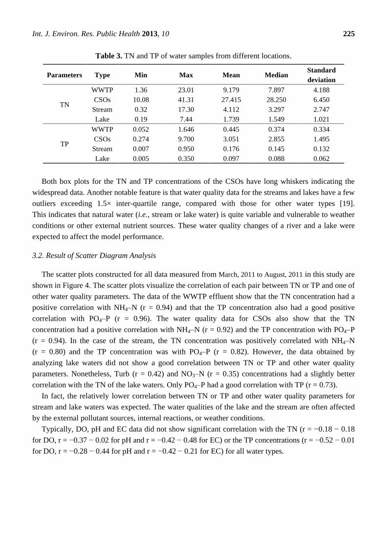
Table 3. TN and TP of water samples from different locations.

Parameters Type Min Max Mean Median Standard

deviation

TN

WWTP 1.36 23.01 9.179 7.897 4.188

CSOs 10.08 41.31 27.415 28.250 6.450

Stream 0.32 17.30 4.112 3.297 2.747

Lake 0.19 7.44 1.739 1.549 1.021

TP

WWTP 0.052 1.646 0.445 0.374 0.334

CSOs 0.274 9.700 3.051 2.855 1.495

Stream 0.007 0.950 0.176 0.145 0.132

Lake 0.005 0.350 0.097 0.088 0.062

Both box plots for the TN and TP concentrations of the CSOs have long whiskers indicating the

widespread data. Another notable feature is that water quality data for the streams and lakes have a few

outliers exceeding 1.5× inter-quartile range, compared with those for other water types [19].

This indicates that natural water (i.e., stream or lake water) is quite variable and vulnerable to weather

conditions or other external nutrient sources. These water quality changes of a river and a lake were

expected to affect the model performance.

3.2. Result of Scatter Diagram Analysis

The scatter plots constructed for all data measured from March, 2011 to August, 2011 in this study are

shown in Figure 4. The scatter plots visualize the correlation of each pair between TN or TP and one of

other water quality parameters. The data of the WWTP effluent show that the TN concentration had a

positive correlation with NH4–N (r = 0.94) and that the TP concentration also had a good positive

correlation with PO4–P (r = 0.96). The water quality data for CSOs also show that the TN

concentration had a positive correlation with NH4–N (r = 0.92) and the TP concentration with PO4–P

(r = 0.94). In the case of the stream, the TN concentration was positively correlated with NH4–N

(r = 0.80) and the TP concentration was with PO4–P (r = 0.82). However, the data obtained by

analyzing lake waters did not show a good correlation between TN or TP and other water quality

parameters. Nonetheless, Turb (r = 0.42) and NO3–N (r = 0.35) concentrations had a slightly better

correlation with the TN of the lake waters. Only PO4–P had a good correlation with TP (r = 0.73).

In fact, the relatively lower correlation between TN or TP and other water quality parameters for

stream and lake waters was expected. The water qualities of the lake and the stream are often affected

by the external pollutant sources, internal reactions, or weather conditions.

Typically, DO, pH and EC data did not show significant correlation with the TN (r = −0.18 − 0.18

for DO, r = −0.37 − 0.02 for pH and r = −0.42 − 0.48 for EC) or the TP concentrations (r = −0.52 − 0.01

for DO, r = −0.28 − 0.44 for pH and r = −0.42 − 0.21 for EC) for all water types.


Figure 4. Scatter plots of water quality parameters for four water types.

(A: WWTP effluent, B: CSOs water, C: stream water, D: lake water).

3.3. Multiple Linear Regression Analysis for Each Water Types

3.3.1. MLR Analysis for WWTP Effluent

With the datasets for the WWTP effluent, the stepwise MLR analysis was conducted. The result of

the regression analysis is summarized in Table 4. For the MRL analysis, the TN and TP concentrations

were set as dependent variables, and the most dominant parameters were initially considered as the

only independent variable for each regression model, with other significant independent variables


added one by one. As the number of independent variables increased from 1 to 3 in the model for the

TN estimation, the 𝑅𝑎2 value also increased gradually. However, if one of the other variables which did

not have a good correlation with the TN was added, the 𝑅𝑎2 value of the regression was deteriorated.

ModelN-3 for estimating TN in Table 4 showed the best fit to the measured TN data (𝑅𝑎2 = 0.978),

while ModelP-1 for estimating TP, which included only PO43−

–P data as independent variable showed

the best fit to the measured TP data (𝑅𝑎2 = 0.936). In short, as a result of these analyses, it was

concluded that the TN and TP concentrations of the WWTP effluent are feasible parameters that can

be estimated using a software sensor. This is mainly due to the fact that the water quality of the

WWTP discharge is relatively stable, compared with natural waters. In fact, the effluent water quality

of a WWTP does not change much as long as the WWTP is operated at steady state. In addition, the

high degree of correlation between PO4–P and TP in the WWTP effluent indicates that most of the

phosphorus species in the effluent were in the dissolved form rather than in particulate ones.

Table 4. Variance analysis of models predicting TN and TP of WWTP effluent.

TN (Dependent variable) TP (Dependent variable)

Model Mean square 𝑹𝒂𝟐 p-value Model Mean square 𝑹𝒂

𝟐 p-value

ModelN-1 a

ModelN-2 b

ModelN-3 c

552.371

305.321

204.081

0.882

0.975

0.978

<0.01

<0.01

<0.01 ModelP-1 a 4.582 0.936 <0.01

Independent variables

a NH4–N

b NH4–N, NO3–N

c NH4–N, NO3–N, PO4–P


a PO4–P

3.3.2. MLR Analysis for CSOs Water

With the water quality parameters measured for CSOs waters, the stepwise MLR analysis was

conducted. The result of the analysis is summarized in Table 5.

Table 5. Variance analysis of models predicting TN and TP of CSOs.



𝟐 p-value

ModelN-1 a

ModelN-2 b

3518.589

1781.741

0.858

0.869

<0.01

<0.01

ModelP-1 a

ModelP-2 b

325.279

165.252

0.902

0.917

<0.01

<0.01


a NH4–N

b NH4–N, PO4–P


a PO4–P

b PO4–P, NH4–N

From the scatter plots for the CSOs water, five variables (i.e., NH4–N, PO4–P, Turb, NO3–N, and

DO) were found to have significant correlation with the measured TN concentration, while three

variables (i.e., PO4–P, DO, NO3–N) were significantly correlated with the TP concentration. However,

the MLR analysis showed that the models with one independent variable (i.e., NH4–N) and two (i.e.,

NH4–N and PO4–P) showed the best fit to the measured TN. ModelN-1 with one dependent variable

showed the 𝑅𝑎2 of 0.858 while ModelN-2 did the 𝑅𝑎

2 of 0.869. In the case of models for the prediction of


TP, PO4–P was identified as the most important variable. The ModelP-2 which has two variables (i.e.,

NH4–N and PO4–P) showed the highest 𝑅𝑎2 value (= 0.917). The result showed that the contribution of

other variables to the prediction of the TP of CSOs might not be significant.

3.3.3. MRL Analysis for Stream Water

Using the water quality data for stream waters, a stepwise MRL analysis was carried out.

The summary of the analysis is provided in Table 6. Since NH4–N was identified as the dominant

variable in the estimation of TN concentration, the regression model was expanded from the one with

NH4-N as the only independent variable to the ones with NO3–N, Turb, PO4–P, pH, NO2–N, and EC in

a stepwise manner. In short, ModelN-7 with NH4–N, NO3–N, Turb, PO4–P, pH, NO2–N, and EC as

independent variables showed the best fit to the measured TN concentration. Therefore, the model was

chosen as the software sensor to estimate TN in stream waters. For the TP concentration, ModelP-6

showed the best fit to the measured TP data, although the 𝑅𝑎2 value was only 0.746; over 70% of the

measured data could be explained by the model. One of the major reasons that low 𝑅𝑎2 value was

obtained might be the low TP concentration of the stream waters; the TP of all the stream water

samples was below 1.0 mg·L−1

with the majority below 0.5 mg·L−1

(Figure 3). At such a low

concentration, errors from manual measurements also may contribute to the error from the model

predictions.

Table 6. Variance analysis of models predicting TN and TP of stream water.



𝟐 p-value

ModelN-1 a

ModelN-2 b

ModelN-3 c

ModelN-4 d

ModelN-5 e

ModelN-6 f

3135.004

2001.062

1361.633

1026.397

827.979

693.635

0. 633

0.808

0.825

0.829

0.836

0.840

<0.01

<0.01

<0.01

<0.01

<0.01

<0.01

ModelP-1 a

ModelP-2 b

ModelP-3 c

ModelP-4 d

ModelP-5 e

ModelP-6 f

8.892

4.759

3.244

2.440

1.957

1.636

0.675

0.723

0.739

0.741

0.743

0.746

<0.01

<0.01

<0.01

<0.01

<0.01

<0.01


a NH4–N

b NH4–N, NO3–N

c NH4–N, NO3–N, Turb

d NH4–N, NO3–N, Turb ,EC,

e NH4–N, NO3–N, Turb, EC, NO2–N,

f NH4–N, NO3–N, Turb, EC, NO2–N, pH,


a PO4–P

b PO4–P, Turb

c PO4–P, Turb, NH4–N

d PO4–P, Turb, NH4–N, NO2–N

e PO4–P, Turb, NH4–N, NO2–N, NO3–N

f PO4–P, Turb, NH4–N, NO2–N, NO3–N, pH

3.3.4. MLR Analysis for Lake Water

Using the water quality data for water samples collected from the lake of interest, the stepwise

MLR analysis was conducted. The summary of the results is provided in Table 7. Unlike the other

cases, any of the models developed through the MRL analyses did not show a good fit to the measured

TN. It is because the TN concentration of the lake water was not well correlated with any other water

quality parameters (Figure 4). The best fit model for the TN estimation was identified ModelN-2 with

Turb, and NO3-N as independent variables (𝑅𝑎2 = 0.417).


The case for predicting TP concentration was similar to the one for TN. The model with PO4–P,

EC, and NO3-N as independent variables (i.e., Model-3) showed the best fit to the measured TP with

the 𝑅𝑎2

of 0.612. One thing of interest is that the model with EC as the only independent variable

showed a comparable 𝑅𝑎2 value with the ModelP-3, indicating the EC data correlated with the TP

concentration.

Again, as the case with the stream waters, the TP concentrations of lake waters was too low; all the

data was below 0.5 mg·L−1

. Therefore, it was hypothesized that errors from manual measurements

might affect the overall predictability of the models.

Table 7. Variance analysis of models predicting TN and TP of lake water.

TN(Dependent Variable) TP(Dependent Variable)


𝟐 p-value

ModelN-1 a

ModelN-2 b

64.883

38.921

0.348

0.417

<0.01

<0.01

ModelP-1 a

ModelP-2 b

ModelP-3 c

.305

.160

.109

0.572

0.599

0.612

<0.01

<0.01

<0.01


a Turb

b Turb, NO3–N


a PO4–P

b PO4–P, EC

c PO4–P, EC, NO3–N

3.3.5. Summary of MRL Analyses for Different Water Types

The best regression models for TN and TP derived from each MLR analysis for each water type are

listed in Table 8.

Table 8. Software sensors obtained from MLR analysis.

Sites Estimated parameters Correlation equations 𝑅𝑎2

WWTP effluent TN 0.881 + 0.986 × NH4–N + 1.092 × NO3–N + 0.631 × PO4–P 0.978

TP 0.148 + 0.946 × PO4–P 0.936

CSOs TN 5.918 + 0.857 × NH4–N + 0.405 × PO4–P 0.869

TP 0.500 + 0.851 × PO4–P + 0.04 × NH4–N 0.917

Stream water

TN 4.569 + 1.025 × NH4–N + 0.838 × NO3–N + 0.018 × Turb −

0.004 × EC + 5.432 × NO2–N − 0.336 × pH 0.840

TP 0.171 + 0.964 × PO4–P + 0.002 × Turb + 0.008 × NH4–N +

0.190 × NO2–N − 0.01 × NO3–N − 0.013 × pH 0.746

Lake water TN 0.361 + 0.158 × Turb + 0.693 × NO3–N 0.417

TP 0.158 + 0.962 × PO4–P − 0.001 × EC − 0.017×NO3–N 0.612

These regression equations can be used as a software sensor. As stated above, the equations for the

WWTP effluent and CSOs water have higher 𝑅𝑎2 values, but the ones for the stream and lake waters

showed a relatively lower relationship for the measured TN and TP concentrations, probably due to

their variability in properties of dissolved or particulate fraction. On the other hand, WWTP effluent

and CSOs have relatively stable water quality compared with natural water; hence, regression models


with higher 𝑅𝑎2 values could be obtained. Figure 5 shows the variations of PO4–P and TP

concentrations for each water type. While WWTP effluent and CSOs show relatively stable ratios

between PO4–P and TP, the ratios of PO4–P to TP concentrations vary to some extent in stream and

lake waters. This might be due to the possibility that particulate phosphorus was introduced from

external sources into the stream and the lake.

Figure 5. Comparison of PO4–P and TP concentrations for each water type.

Comparisons between measured TN or TP concentrations and those predicted by the software

sensors for each water type were made in Figures 6 and 7 for TN and TP, respectively.

For the validation of the developed models, the regression models were applied to another set of

measured water quality data for each water type collected from September 2011 to June 2012.

10 20 30 40 50 60 70

P C

on

c.(m

g/L

)

0.0

0.5

1.0

1.5

2.0

TP Conc.

PO4-P Conc.

30 60 90 120 150 180 210 240

P C

on

c.(m

g/L

)

0

2

4

6

8

10

No. of data

30 60 90 120 150 180 210

P C

on

c.(m

g/L

)

0.0

0.1

0.2

0.3

0.4150 300 450 600 750 900 1050 1200

P C

on

c.(m

g/L

)

0.0

0.2

0.4

0.6

0.8

1.0

WWTP effluent

Stream water

CSOs

Lake water


As shown in Figures 8 and 9, the regression models developed in this study showed relatively good

estimation for the WWTP effluent and CSOs. However, the ones for the stream and lake waters did

relatively lower predictability. For streams and lakes, we would have obtained better results if we had

calibrated the model for each season. In fact, we did not have enough data to do the seasonal analysis

for the stream and the lake. In addition, most sampling stations for the stream and the lake had been

frozen often during the winter season. If the ionic N and P species could be in situ monitored along

with other physical parameters for river and lake waters in this study, and enough data could be

obtained to utilize for model calibration within short period of time, we believe better predictions of

TN and TP could be possible.

Figures 10 and 11 represent the time series of TN and TP concentrations estimated using the

software sensors (or regression models) derived in this study along with measured data. As discussed

above, the models follow the measured data well in the case of the WWTP effluent and the CSOs.

In fact, the models for TN and TP of the stream and lake waters also reasonably follow the measured

data except several points. If the time interval for data collection can be shortened, these intermittently

occurring discrepancies between measured and predicted TN or TP values might be eliminated.

Figure 6. Comparison of measured and estimated TN concentrations for each water type.

WWTP effluent

Lake waterStream water

CSOs

R2 = 0.978 R2 = 0.869

R2 = 0.840 R2 = 0.418


Figure 7. Comparison of measured and estimated TP concentrations for each water type.

Figure 8. Validation of TN models for each water type.

R2 =0. 935 R2 = 0.917

R2 =0. 746 R2 =0. 612

WWTP effluent


CSOs

R2 = 0.953 R2 = 0.670

R2 = 0.624 R2 = 0.047

WWTP effluent


CSOs


Figure 9. Validation of TP models for each water type.

Figure 10. Time series of TN concentration predicted by software sensor.

R2 =0. 865 R2 = 0.553

R2 =0. 651 R2 =0. 122

WWTP effluent


CSOs


Figure 11. Time series of TP concentration predicted by software sensor.

4. Conclusions

In this study, software sensors (or linear regression models) based on the MLR analysis algorithms

were developed; they utilized other water quality parameters for predicting TN and TP concentrations

of WWTP effluent, CSOs, stream water, and lake water. Initially, a few independent variables such as

pH, DO, EC, Turb, NO2–N, NO3–N, NH4–N, and PO4–P concentrations were evaluated for their

individual correlation with TN or TP; the variables with higher correlation with TN and TP were

incorporated in the software sensors (or regression models) as an independent variables.

In fact, the developed software sensors predicted the TN and TP concentrations for the WWTP

effluent and CSOs waters reasonably well. In the case of the stream and lake waters, the predictability

of the software sensors was relatively low, probably due to the low concentration ranges for the

nutrients (especially for the TP) and variability of the ratios of PO4–P to TP concentrations due to the

external influence to the water bodies, such as nonpoint source pollution or weather changes.

From the result, nonetheless, it is expected that the proposed strategy (i.e., application of a software

sensor to monitor TN or TP) will allow the water researchers to monitor TN and TP in various water

bodies more easily; especially for WWTP discharges and CSOs. If all the water quality parameters

used as dependent variables for the regression models are analyzed in situ (as the case in the National

Automated Water Quality Monitoring Program in Korea [20]), the software sensors for TN and TP can

be easily realized and the two water quality parameters which are difficult to measure can be estimated

continuously.

Date04/01/11 06/01/11 08/01/11 10/01/11 12/01/11 02/01/12 04/01/12 06/01/12

TP

Con

c.(m

g/L

)

0.0

0.5

1.0

1.5

2.0

Date04/01/11 06/01/11 08/01/11 10/01/11 12/01/11 02/01/12 04/01/12 06/01/12

TP

Con

c.(m

g/L

)

0

2

4

6

8

10

Measured Value

Calculated Value

Date04/01/11 06/01/11 08/01/11 10/01/11 12/01/11 02/01/12 04/01/12 06/01/12

TP

Con

c.(m

g/L

)

0.0

0.1

0.2

0.3

0.4

0.5

Date04/01/11 06/01/11 08/01/11 10/01/11 12/01/11 02/01/12 04/01/12 06/01/12

TP

Con

c.(m

g/L

)

0.0

0.1

0.2

0.3

0.4

0.5

WWTP effluent

Stream water

CSOs

Lake water


Acknowledgment

This work was supported by the R&D program of MKE/KEIT (R&D program number: 10037331,

Development of Core Water Treatment Technologies based on Intelligent BT-NT-IT Fusion Platform).

References

1. Cesil, D.; Kozlowska, M. Software sensors are a real alternative to true sensors. Environ. Model.

Software 2010, 25, 622–625.

2. Bourgeois, W.; Burgess, J.R.; Stuetz, R.M. On-line monitoring of wastewater quality: A review.

J. Chem. Technol. Biotechnol. 2001, 76, 337–348

3. Sotomayer, O.A.Z.; Park, S.W; Garcia, C. Software sensor for on-line estimation of the microbial

activity in activated sludge systems. ISA Trans. 2010, 41, 127–143.

4. Jansson, A.; Rottorp, J.; Rahmberg, M. Development of a software sensor for phosphorus in

municipal wastewater. J. Chemometr. 2002, 16, 542–547.

5. Christensen, V.G.; Ziegler, A.C.; Jian, X. Continuous Turbidity Monitoring and Regression

Analysis to Estimate Total Suspended Solids and Fecal Coliform Bacteria Loads in Real Time;

US Geological Survey: Reston, VA, USA, 2008.

6. Christensen, V.G.; Rasmussen, P.P.; Ziegler, A.C. Real-Time Water-Quality Monitoring and

Regression Analysis to Estimate Nutrient and Bacteria Concentrations in Kansas Stream; US

Geological Survey: Reston, VA, USA, 2008.

7. Uhrich, M. Comparison of Suspended-Sediment Load Estimates Using a Turbidity and

Suspended-Sediment Concentration Regression and the Graphical Constituent Loading Analysis

System. In Proceedings of the Eighth Federal Interagency Sedimentation Conference, Reno, NV,

USA, 2–6 April 2006,

8. Zhu, Y.; Day, R.L. Regression modeling of steamflow, baseflow, and runoff using geographic

information systems. J. Environ. Manag. 2009, 90, 946–953.

9. Alastair, W.; Hobbs, P.; Holliman, P.; Ravella, S.R.; Pardo, G.; Williams, J.; Retter, A. Software

Sensor Monitoring and Expert Control of Biogas Production. In Proceedings of the 13th

RAMIRAN International Conference, Albena, Bulgaria, June 2008; pp. 121–125.

10. Alcaraz-Gonzalez, V.; Harmand, J.; Rapaport, A.; Steyer, J.P.; Gonzalez-Alvarez, V.;

Pelayo-Ortiz, C. Software sensors for highly uncertain waste water treatment plants: A new

approach based on interval observers. Water Res. 2002, 36, 2515–2524.

11. Feitkenhauer, H.; Meyer, U. Software sensors based on titrimetric techniques for the monitoring

and control aerobic and anaerobic bioreactors. Biochem. Eng. J. 2004, 17, 147–151.

12. Jeong, H.-S.; Lee, S.-H.; Shin, H.-S. Feasibility of on-line measurement of sewage components

using the UV absorbance and the neural network. Environ. Monit. Assess. 2007, 133, 15–24.

13. da Costa, A.O.S.; Silva, P.F.; Sabará, M.G.; da Costa, E.F., Jr. Use of neural networks for

monitoring surface water quality changes in a neotropical urban stream. Environ. Monit. Assess.

2009, 155, 527–538.


14. Ryberg, K.R. Continuous Water-quality Monitoring and Regression Analysis to Estimate

Constituent Concentrations and Loads in the Red River of the North, Fargo, North Dakota, US

Geological Survey: Reston, VA, USA, 2006.

15. Christensen, V.G.; Rasmussen, P.P.; Ziegler, A.C. Real-time water quality monitoring and

regression analysis to estimate nutrient and bacteria concentrations in Kansas streams. Water Sci.

Technol. 2002, 45, 205–211.

16. Moore, D.; McCabe, G.P.; Craig, B. Introduction to the Practice of Statistics, 6th ed.; Freeman:

New York, NY, USA, 2009.

17. Burnham, K.P.; Anderson, D.R. Model Selection and Multimodel Inference: A Practical

Information-Theoretic Approach, 2nd ed.; Springer: New York, NY, USA, 2002.

18. IBM SPSS Statistics 20 Core System User’s Guide. IBM Software Group: Armonk, NY, USA,

2011.

19. Massart, D.L.; J.; Verbeke, S.; Capron, X.; Schlesier, K. Visual presentation of data by means of

box plots. LC-GC Eur. 2005, 18, 215–218.

20. Kim, H.; Lim, B.J.; Lee, S.; Colosimo, M.F. On-Line Monitoring Systems Supporting an

Adaptively Managed Water Conservation Policy in South Korea. In Proceedings of the American

Water Resources Association 2009 Summer Specialty Conference—Adaptive Management of

Water Resources II, Snowbird, UT, USA, June 29–July 1 2009.

© 2013 by the authors; licensee MDPI, Basel, Switzerland. This article is an open access article

distributed under the terms and conditions of the Creative Commons Attribution license

(http://creativecommons.org/licenses/by/3.0/).

Development of Software Sensors for Determining Total Phosphorus and Total Nitrogen in Waters

Documents

Transcript of Development of Software Sensors for Determining Total Phosphorus and Total Nitrogen in Waters