Development of Scientifically-Based Planning Standards and ...
91
Development of Scientifically-Based Planning Standards and Test Methods to Predict Effectiveness and Usage Rates for Surface and Subsea Dispersant Use in Various Types of Environmental Conditions Prepared by M. Scott Miles, Puspa Adahkari, and Brittany Cheschister Department of Environmental Sciences Louisiana State University Prepared for Bureau of Safety and Environmental Enforcement U.S. Department of Interior This study was funded by the Bureau of Safety and Environmental Enforcement (BSEE), U.S. Department of Interior, Washington, D.C., under Contract #E14PC00019 January 31, 2016
Transcript of Development of Scientifically-Based Planning Standards and ...
Development of Scientifically-Based Planning Standards and Test Methods to Predict Effectiveness and Usage Rates for Surface and Subsea Dispersant Use
in Various Types of Environmental Conditions
Prepared by M. Scott Miles, Puspa Adahkari, and Brittany Cheschister
Department of Environmental Sciences Louisiana State University
Prepared for Bureau of Safety and Environmental Enforcement
U.S. Department of Interior
This study was funded by the Bureau of Safety and Environmental Enforcement (BSEE), U.S. Department of Interior, Washington, D.C., under Contract #E14PC00019
January 31, 2016

ACKNOWLEDGEMENTS
The authors wish to thank Mr. Adam Davis and Dr. Paige Doelling from the National Oceanic and Atmospheric Administration (NOAA) and CDR Kevin Lynn from the United States Coast Guard (USCG) Gulf Coast Strike Team for providing valuable feedback and recommendations on the project.
DISCLAIMER
This final report has been reviewed by the Bureau of Safety and Environmental Enforcement (BSEE) and approved for publication. Approval does not signify that the contents necessarily reflect the views and policies of the BSEE, nor does mention of the trade names or commercial products constitute endorsement or recommendation for use.
i
TABLE OF CONTENTS
ACKNOWLEDGEMENTS............................................................................................................. i
Disclaimer ........................................................................................................................................ i
Table of contents............................................................................................................................. ii
LIST OF FIGURES ....................................................................................................................... iii
LIST OF TABLES.......................................................................................................................... v
EXECUTIVE SUMMARY ............................................................................................................ 1
Introduction..................................................................................................................................... 2
Problem Statement .......................................................................................................................... 4
Project Description.......................................................................................................................... 8
Research Goal ................................................................................................................................. 9
MATERIALS AND METHODS.................................................................................................. 10
Experimental Oil Characterization and Dispersant .................................................................. 10
Synthetic Water Preparation ..................................................................................................... 11
Analytical Instrumentation ....................................................................................................... 12
Preparation of Crude Oil Standards .......................................................................................... 12
Oil Extraction and Analysis...................................................................................................... 13
Analysis of Sample Extracts ..................................................................................................... 15
Statistical Analysis .................................................................................................................... 16
Task #1: 150-ml Baffled Flask Test Study ............................................................................... 18
Results & Discussion: 150-ml Baffled Flask Tests .................................................................. 20
Task #2: Pressure Vessel Study ................................................................................................ 28
Results & Discussion: Pressure Vessel Study .......................................................................... 32
Task #3: 1-L Baffled Flask Test Study..................................................................................... 37
Results & Discussion: 1-L Baffled Flask Tests ........................................................................ 41
Summary of Key Results and Recommendations ......................................................................... 55
References..................................................................................................................................... 57
APPENDIX................................................................................................................................... 58
ii

LIST OF FIGURES
Figure 1. Photographs of Aqualog spectrofluorometer (top), Turner Designs Cyclops-7 probe (mid), and Hach portable turbidimeter (bottom). ............................................................... 14
Figure 2 Normalized intensity contour plots of excitation-emission matrix spectra (EEMs) of South Louisiana, North Slope, and Hondo crude oils. ............................................................. 17
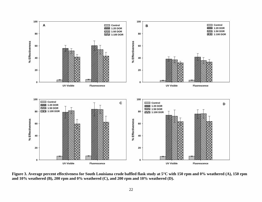
Figure 3. Average percent effectiveness for South Louisiana crude baffled flask study at 5°C with 150 rpm and 0% weathered (A), 150 rpm and 10% weathered (B), 200 rpm and 0% weathered (C), and 200 rpm and 10% weathered. ........................................................................ 22
Figure 4. Average percent effectiveness for South Louisiana crude baffled flask study at 23°C with 150 rpm and 0% weathered (A), 150 rpm and 10% weathered (B), 200 rpm and 0% weathered (C), and 200 rpm and 10% weathered. .................................................................. 23
Figure 5. Average percent effectiveness for North Slope crude baffled flask study at 5°C with 150 rpm and 0% weathered (A), 150 rpm and 10% weathered (B), 200 rpm and 0% weathered (C), and 200 rpm and 10% weathered. ........................................................................ 24
Figure 6. Average percent effectiveness for North Slope crude baffled flask study at 23°C with 150 rpm and 0% weathered (A), 150 rpm and 10% weathered (B), 200 rpm and 0% weathered (C), and 200 rpm and 10% weathered. ........................................................................ 25
Figure 7. Average percent effectiveness for Hondo crude baffled flask study at 5°C with 150 rpm and 0% weathered (A), 150 rpm and 10% weathered (B), 200 rpm and 0% weathered (C), and 200 rpm and 10% weathered. ........................................................................ 26
Figure 8. Average percent effectiveness for Hondo crude baffled flask study at 23°C with 150 rpm and 0% weathered (A), 150 rpm and 10% weathered (B), 200 rpm and 0% weathered (C), and 200 rpm and 10% weathered. ........................................................................ 27
Figure 9. Experimental design for the determination of dispersant effectiveness in water at elevated pressures. .................................................................................................................... 29
Figure 10. Photographs of high-pressure vessel and pumping system. ........................................ 30
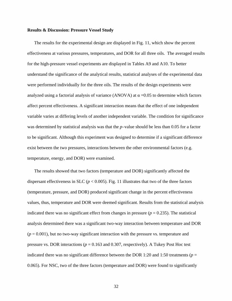
Figure 11. Average percent effectiveness for South Louisiana, North Slope, and Hondo crude baffled flask study at 23°C and 200 psi (A), 23°C and 2000 psi (B), 5°C and 200 psi (C), and 5°C and 2000 psi............................................................................................................. 36
Figure 12. Average percent effectiveness for South Louisiana crude baffled flask study at 5°C with 150 rpm and 0% weathering (A), 150 rpm and 10% weathering (B), 200 rpm and 0% weathering (C), and 200 rpm and 10% weathering. ............................................................... 46
Figure 13. Average percent effectiveness for South Louisiana crude baffled flask study at 23°C with 150 rpm and 0% weathering (A), 150 rpm and 10% weathering (B), 200 rpm and 0% weathering (C), and 200 rpm and 10% weathering (D). ........................................................ 47
Figure 14. Average percent effectiveness for North Slope crude baffled flask study at 5°C with 150 rpm and 0% weathering (A), 150 rpm and 10% weathering (B), 200 rpm and 0% weathering (C), and 200 rpm and 10% weathering (D). ............................................................... 48
iii

LIST OF FIGURES (continued)
Figure 15. Average percent effectiveness for North Slope crude baffled flask study at 23°C with 150 rpm and 0% weathering (A), 150 rpm and 10% weathering (B), 200 rpm and 0% weathering (C), and 200 rpm and 10% weathering (D). ............................................................... 49
Figure 16. Average percent effectiveness for Hondo crude baffled flask study at 5°C with 150 rpm and 0% weathering (A), 150 rpm and 10% weathering (B), 200 rpm and 0% weathering (C), and 200 rpm and 10% weathering (D)............................................................... 50
Figure 17. Average percent effectiveness for Hondo crude baffled flask study at 23°C with 150 rpm and 0% weathering (A), 150 rpm and 10% weathering (B), 200 rpm and 0% weathering (C), and 200 rpm and 10% weathering (D). ............................................................... 51
Figure A1. Laboratory Fluorescence Curves: (A) South Louisiana crude, (B) North Slope crude, and (C) Hondo crude.......................................................................................................... 81
Figure A2. Laboratory UV-Vis Curves: (A) South Louisiana crude, (B) North Slope crude, and (C) Hondo crude.......................................................................................................... 82
Figure A3. Field Probe Calibration Curves: (A) South Louisiana crude, (B) North Slope crude, and (C) Hondo crude. Baseline: DOR=1:20, 23°C, and 150 rpm...................................... 83
Figure A4. Turbidimeter Calibration Curves: (A) South Louisiana crude, (B) North Slope crude, and (C) Hondo crude. Baseline: DOR=1:20, 23°C, and 150 rpm...................................... 84
iv

LIST OF TABLES
Table 1. Physical Properties of the Oils Used in the Experiments ............................................... 11
Table 2. Correction factors for oils and field conditions. ............................................................. 43
Table 3. Predicted dispersant effectiveness equation for South Louisiana, North Slope, and Hondo crude oils at baseline conditions ....................................................................................... 44
Table 4. List of Personnel Attending the 1-Day Dispersant Workshop ....................................... 53
Table A1. 150-ml Baffled Flask Percent Effectiveness Results (fluorescence) at 5°C ................... and 150 rpm. ................................................................................................................................. 59
Table A2. 150-ml Baffled Flask Percent Effectiveness Results (fluorescence) at 5°C and 200 rpm. ................................................................................................................................. 60
Table A3. 150-ml Baffled Flask Percent Effectiveness Results (fluorescence) at 23°C and 150 rpm. ................................................................................................................................. 61
Table A4. 150-ml Baffled Flask Percent Effectiveness Results (fluorescence) at 23°C and 200 rpm. ................................................................................................................................ 62
Table A5. 150-ml Baffled Flask Percent Effectiveness Results (UV-Vis) at 5°C and 150 rpm. ................................................................................................................................. 63
Table A6. 150-ml Baffled Flask Percent Effectiveness Results (UV-Vis) at 5°C and 200 rpm. ................................................................................................................................. 64
Table A7. 150-ml Baffled Flask Percent Effectiveness Results (UV-Vis) at 23°C and 150 rpm. ................................................................................................................................. 65
Table A8. 150-ml Baffled Flask Percent Effectiveness Results (UV-Vis) at 23°C and 200 rpm. ................................................................................................................................. 66
Table A9. 1-L Pressure Vessel Percent Effectiveness Results (A) 5°C @ 200 psi and (B) 5°C @ 2000 psi................................................................................................................ 67
Table A10. 1-L Pressure Vessel Percent Effectiveness Results (A) 23°C @ 200 psi and (B) 23°C @ 2000 psi.............................................................................................................. 68
Table A11. 1-L Baffled Flask Percent Effectiveness Results (laboratory fluorescence) 5°C @ 150 rpm. ............................................................................................................................ 69
Table A12. 1-L Baffled Flask Percent Effectiveness Results (laboratory fluorescence) 5°C @ 200 rpm. ............................................................................................................................ 70
Table A13. 1-L Baffled Flask Percent Effectiveness Results (laboratory fluorescence) 23°C @ 150 rpm. .......................................................................................................................... 71
Table A14. 1-L Baffled Flask Percent Effectiveness Results (laboratory fluorescence) 23°C @ 200 rpm. .......................................................................................................................... 72
Table A15. 1-L Baffled Flask Percent Effectiveness Results (probe fluorescence) 5°C @ 150 rpm. ............................................................................................................................ 73
v

LIST OF TABLES (continued)
Table A16. 1-L Baffled Flask Percent Effectiveness Results (probe fluorescence) 5°C @ 200 rpm. ............................................................................................................................ 74
Table A17. 1-L Baffled Flask Percent Effectiveness Results (probe fluorescence)
Table A18. 1-L Baffled Flask Percent Effectiveness Results (probe fluorescence)
23°C @ 150 rpm ........................................................................................................................... 75
23°C @ 200 rpm. .......................................................................................................................... 76
Table A19. 1-L Baffled Flask Percent Effectiveness Results (turbidity) 5°C @ 150 rpm. .......... 77
Table A20. 1-L Baffled Flask Percent Effectiveness Results (turbidity) 5°C @ 200 rpm. .......... 78
Table A21. 1-L Baffled Flask Percent Effectiveness Results (turbidity) 23°C @ 150 rpm. ........ 79
Table A22. 1-L Baffled Flask Percent Effectiveness Results (turbidity) 23°C @ 200 rpm. ........ 80
vi

EXECUTIVE SUMMARY
The fundamental goal of oil spill planning is to reduce the ecological and socioeconomic
impacts of a spill to a minimum. Since the early 1980s oil spill response planning and operations
have focused primarily on identifying qualified personnel, procuring available equipment, and
establishing proper lines of communication to combat the effects of oil spill disasters. Much time
and work has been focused on resources at risks and evaluating the ecological implications of
cleanup methods and the pros and cons associated with these methods. The oil spill community
(industry, government agencies, and universities) has developed many guidelines and protocols
for the planning and management of oil spill incidents, primarily focusing on spill management,
control measures (e.g. skimming, booming, and dispersing) and enhancing the remediation
decision-making process. There has been very little scientifically-based planning for
standardization of dispersant effectiveness and usage rate guidelines for oil spill incidents. The
American Society for Testing and Materials (ASTM) and American Petroleum Institute (API)
have organized multiple agency task forces designed to develop methods for site-specific,
advance planning for dispersant use. The ASTM and API planning guidelines are useful during
oil spills, but primarily focus on habitat prioritization, protection, and cleanup recommendations.
In order to provide a complete analysis of dispersant effectiveness and usage rates testing,
LSU’s Department of Environmental Sciences conducted a one (1) year study to provide detailed
scientific information and data on the development of methodology for testing effectiveness and
determining usage rates for surface and subsea dispersant use in various types of environmental
conditions. The goals of this project were achieved through a series of laboratory studies
conducted at LSU’s Department of Environmental Sciences’ Response and Chemical
Assessment Team (RCAT) laboratory. Subsequently, a 1-day workshop presenting the final
1

results and protocol was held at NOAA’s Gulf of Mexico Disaster Response Center in Mobile,
Alabama. Attendees included oil spill representatives from BSEE, LSU, NOAA’s Emergency
Response Division (ERD), and the USCG Gulf Strike Team.
INTRODUCTION
Our coastal shorelines and saltwater marshes accommodate a diverse range of vegetative,
aquatic, and mammalian habitats. For this reason, large amounts of resources are devoted to
preventing offshore oil spills from impacting near shore environments. In calm and pristine sea
conditions, booming and skimming techniques are the preferred cleanup and recovery
methodology. In situ burning is another cleanup option, but is limited to condensed spills which
produce a more intense and complete burn. In situ burning also produces large plums of harmful
smoke and tends to leave residual oil within the water column. Unfortunately, inclement weather
is often encountered during oil spills making sea conditions less than optimum for these cleanup
techniques. In rough seas, chemical dispersants appear to be the most effective cleanup tool for
removing spilled oil from the water surface. Dispersant application is primarily a spill control
method designed to remove the oil from the water’s surface. Oil spill dispersants are special
blends of surfactants in a carrier solvent. The surfactant is the most effective component of the
mixture and is composed of a compound that contains both oleophilic (non-polar) and
hydrophilic (polar) regions within the same molecule. Surfactants alter the physical and chemical
properties of the oil so that the interfacial tension between the oil and the water surface are
greatly reduced, promoting the formation of small oil droplets. The dispersant, along with wave
energy, breakup the oil slick and force it into the water column as small oil droplets. The
reduction in droplet size increases the oil’s overall surface area, thus enhancing microbial
2
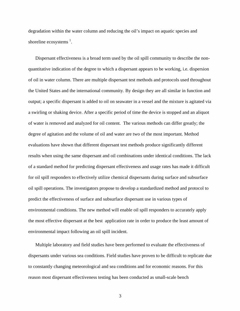
degradation within the water column and reducing the oil’s impact on aquatic species and
shoreline ecosystems 1.
Dispersant effectiveness is a broad term used by the oil spill community to describe the non-
quantitative indication of the degree to which a dispersant appears to be working, i.e. dispersion
of oil in water column. There are multiple dispersant test methods and protocols used throughout
the United States and the international community. By design they are all similar in function and
output; a specific dispersant is added to oil on seawater in a vessel and the mixture is agitated via
a swirling or shaking device. After a specific period of time the device is stopped and an aliquot
of water is removed and analyzed for oil content. The various methods can differ greatly; the
degree of agitation and the volume of oil and water are two of the most important. Method
evaluations have shown that different dispersant test methods produce significantly different
results when using the same dispersant and oil combinations under identical conditions. The lack
of a standard method for predicting dispersant effectiveness and usage rates has made it difficult
for oil spill responders to effectively utilize chemical dispersants during surface and subsurface
oil spill operations. The investigators propose to develop a standardized method and protocol to
predict the effectiveness of surface and subsurface dispersant use in various types of
environmental conditions. The new method will enable oil spill responders to accurately apply
the most effective dispersant at the best application rate in order to produce the least amount of
environmental impact following an oil spill incident.
Multiple laboratory and field studies have been performed to evaluate the effectiveness of
dispersants under various sea conditions. Field studies have proven to be difficult to replicate due
to constantly changing meteorological and sea conditions and for economic reasons. For this
reason most dispersant effectiveness testing has been conducted as small-scale bench
3

experiments. Approximately 50 different laboratory tests methods have been reported for
determining the effectiveness of dispersants on oil. A few of the most popular test methods
include the Exxon dispersant effectiveness test method (EXDET), the French IFP test method,
the Warren Spring Laboratory test method, the swirling flask test (SFT) method, and the baffled
flask test (BFT) method. Until recently the most widely accepted test method throughout the
United States was the SFT method. The SFT method was officially adopted by the US
Environmental Protection Agency (EPA) in 1994 as its official laboratory screening
methodology for determining the effectiveness of dispersants in seawater. Soon after its adoption
unexpected discrepancies were discovered between the data submitted by independent
laboratories and those generated by EPA contract laboratories for numerous dispersant products
on the National Contingency Plan (NCP) schedule list. Within the last decade, a new method has
been adopted by the EPA for the determination of dispersant effectiveness on oil spills. The
Baffled Flask Test (BFT) was developed at the Andrew W. Breidenbach Environmental
Research Center in the National Risk Management Research Laboratory, a division of the U.S.
Environmental Protection Agency’s Office of Research and Development. The BFT has proven
to be substantially more reproducible and repeatable when performed by independent and EPA
laboratories 1. In addition, the BFT is the only available device that has been scientifically
calibrated with respect to mixing energy.
PROBLEM STATEMENT
The fundamental goal of oil spill planning is to reduce the ecological and socioeconomic
impacts of a spill to a minimum. Since the early 1980s oil spill response planning and operations
have focused primarily on identifying qualified personnel, procuring available equipment, and
establishing proper lines of communication to combat the effects of oil spill disasters. Much time
4

and work has been focused on resources at risks and evaluating the ecological implications of
cleanup methods and the pros and cons associated with these methods. The oil spill community
(industry, government agencies, and universities) has developed many guidelines and protocols
for the planning and management of oil spill incidents, primarily focusing on spill management,
control measures (e.g. skimming, booming, and dispersing) and enhancing the remediation
decision-making process. A review of oil spill incidents (i.e. open water) have shown that
mechanical containment and recovery is the primary control measure for reducing ecological and
socioeconomic impacts from oil spills in the United States 2. Some countries almost completely
rely on chemical dispersants contain oil spills because frequently rough or choppy sea conditions
prevent the use mechanical containment and cleanup 3. However, dispersants have not been used
extensively in the United States because of possible long term environmental effects, difficulties
with timely and effective application, disagreement among scientists and research data about
their environmental effects, effectiveness, and toxicity concerns.
There has been very little scientifically-based planning for standardization of dispersant
effectiveness and usage rate guidelines for oil spill incidents. The American Society for Testing
and Materials (ASTM) and American Petroleum Institute (API) have organized multiple agency
task forces designed to develop methods for site-specific, advance planning for dispersant use.
The ASTM and API planning guidelines are useful during oil spills, but primarily focus on
habitat prioritization, protection, and cleanup recommendations. The European Maritime Safety
Agency (EMSA) 4 has developed an international manual on the applicability of oil spill
dispersants. The manual is very detailed and contains data from dispersant effectiveness studies
and operational treatment rates for dispersants. Unfortunately, the tests used in the EMSA
manual are complicated and have limited value when comparing to dispersant effectiveness
5

measurements at sea. The National Contingency Plan (NCP) 5 is the United States
Environmental Protection Agency's (USEPA) blueprint for responding to both oil spills and
hazardous substance releases. The NCP is the result of efforts to develop a national response
capability and promote coordination among the hierarchy of responders and contingency plans.
The plan is quite effective, but is very broad in its guidance and only recommends approved
dispersants, not their predicted effectiveness and usage rates for varying environmental
conditions. The USEPA is currently employing the BFT to determine the effectiveness of
dispersants on oils. The test is effective but does not take into account for variations in
application rates, sea state, or temperature. The BFT shares many of the same limitations as the
SFT, providing ranks rather than absolute effectiveness numbers. The test is not yet standard in
any jurisdiction. Many scientist argue that this test overestimates the effectiveness of dispersants
by making unrealistically large amounts of energy available to the mixture and that real ocean
waves have much less energy available to force the dispersion. Further, no approved analytical
method has yet been chosen for this test. The United States Coast Guard (USCG) and the
National Oceanographic and Atmospheric Administration (NOAA) have employed the Special
Monitoring of Applied Response Technologies (SMART) 6 to monitor dispersant application
during oil spill operations. Again, the current USCG and NOAA protocol does not address
effectiveness and usage rates of specific NCP dispersants. During the most recent large-scale
dispersant application, the Deepwater Horizon spill, an estimated 1.84 million gallons of Corexit
EC9500A and Corexit EC9527A had been applied during surface and subsea operations over a
four (4) month period. During this time period, no official guidance or standard was followed
during dispersant operations. Reports showed that dispersants were applied at usage rates
ranging from 1:10 dispersant to oil ratio (DOR) to as low as 1:200 DOR. The Texas City Y is a
6
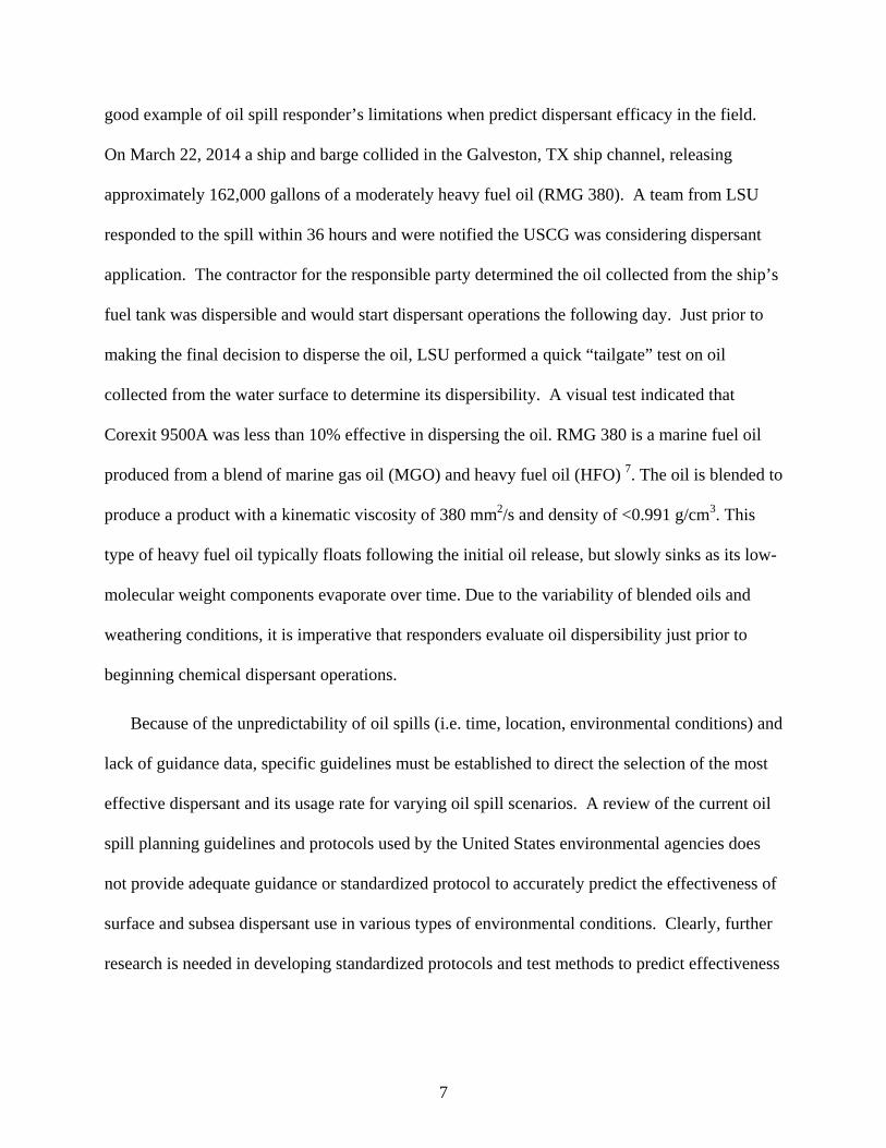
good example of oil spill responder’s limitations when predict dispersant efficacy in the field.
On March 22, 2014 a ship and barge collided in the Galveston, TX ship channel, releasing
approximately 162,000 gallons of a moderately heavy fuel oil (RMG 380). A team from LSU
responded to the spill within 36 hours and were notified the USCG was considering dispersant
application. The contractor for the responsible party determined the oil collected from the ship’s
fuel tank was dispersible and would start dispersant operations the following day. Just prior to
making the final decision to disperse the oil, LSU performed a quick “tailgate” test on oil
collected from the water surface to determine its dispersibility. A visual test indicated that
Corexit 9500A was less than 10% effective in dispersing the oil. RMG 380 is a marine fuel oil
produced from a blend of marine gas oil (MGO) and heavy fuel oil (HFO) 7. The oil is blended to
produce a product with a kinematic viscosity of 380 mm2/s and density of <0.991 g/cm3. This
type of heavy fuel oil typically floats following the initial oil release, but slowly sinks as its low-
molecular weight components evaporate over time. Due to the variability of blended oils and
weathering conditions, it is imperative that responders evaluate oil dispersibility just prior to
beginning chemical dispersant operations.
Because of the unpredictability of oil spills (i.e. time, location, environmental conditions) and
lack of guidance data, specific guidelines must be established to direct the selection of the most
effective dispersant and its usage rate for varying oil spill scenarios. A review of the current oil
spill planning guidelines and protocols used by the United States environmental agencies does
not provide adequate guidance or standardized protocol to accurately predict the effectiveness of
surface and subsea dispersant use in various types of environmental conditions. Clearly, further
research is needed in developing standardized protocols and test methods to predict effectiveness
7

and usage rates for surface and subsea dispersant use in various types of environmental
conditions.
PROJECT DESCRIPTION
The use of dispersants on oil spills has been renewed in the United States by recent high –
profile oil spills (e.g. Deepwater Horizon and Texas City Y) and the increased transport of oil
products within our navigable waterways. Much interest has been generated towards predicting
effectiveness and usage rates for surface and subsea dispersant use in various types of
environmental conditions. The current dispersant effectiveness test, BFT, is effective and its
results are widely documented. Unfortunately, most studies employing the BFT are standardized
and do not investigate variations in temperatures, dispersant-to-oil ratios (DORs), and mixing
energy levels. Recently, Venosa and Holder (2013) conducted a study to determine the
dispersibility of South Louisiana crude oil by eight oil dispersants at multiple water temperatures
(25°C and 5°C). This was one of the few times that a BFT was used to determine dispersibility
of oils at subsea temperatures. Kaku et al. (2006) performed an extensive evaluation of mixing
energy in laboratory flasks used for dispersant effectiveness tests. Their research showed that
the turbulence generated at 200 revolutions per minute (rpm) using the BFT resembled the
turbulence occurring at sea during breaking waves. Again, very few studies have been
conducted investigating variations in mixing energy during dispersant effectiveness testing.
In order to provide a complete analysis of dispersant effectiveness and usage rates testing, LSU’s
Department of Environmental Sciences conducted a one (1) year study to provide detailed
scientific information and data on the development of methodology for testing effectiveness and
determining usage rates for surface and subsea dispersant use in various types of environmental
8
conditions. The goals of this project were achieved through a series of laboratory studies
conducted at LSU’s Department of Environmental Sciences’ Response and Chemical
Assessment Team (RCAT) laboratory. Subsequently, a 1-day workshop presenting the final
results and protocol was held at NOAA’s Gulf of Mexico Disaster Response Center in Mobile,
Alabama. Attendees included oil spill representatives from LSU, NOAA’s Emergency Response
Division (ERD), and the USCG Gulf Strike Team.
RESEARCH GOAL
Response and analytical reports from the Deepwater Horizon and other spill incidents
indicate that the use of dispersant, in both surface and subsurface application, significantly
reduced the shoreline impact of oil following the spills 8,9,10. The lack of current scientifically-
based planning standards for dispersant effectiveness and usage rates during past oil spill
incidents indicates there is a need for further study into development of a standard protocol to
employ during surface and subsurface oil spills. In addition, a universal dispersant effectiveness
and usage rate method (laboratory and field-based) should to be developed to scientifically
validate the standard protocol. In response to the above needs, a joint research team, comprised
of researchers from Louisiana State University’s Department of Environmental Sciences,
USEPA, NOAA, and USCG, propose the development of laboratory and field-based dispersant
effectiveness/usage rate methods and a standardized protocol to assist responders in predicting
the effectiveness of surface and subsurface dispersant use in various environmental conditions.
The goal of this study were accomplished through a series of five (5) research objectives: (1)
Evaluation of multiple oils under varying environmental and physical conditions (temperature,
rotational energy level, weathering state, and dispersant usage rate) using the standardized BFT,
(2) Evaluation of multiple oils under varying environmental and physical conditions
9

(temperature, pressure, and dispersant usage rate) using a 1-liter stainless steel pressure vessel
equipped with an integrated paddle stirrer, (3) Development of a 1-L baffled flask test protocol to
predict the effectiveness of dispersantson multiple oils using an in situ fluorescence probe and
turbidity meter, (4) Organize a 1-day dispersant workshop to discuss project results and
determine if a field deployable 1-L BFT methodology can enhance current SMART protocol,
and (5) Preparation and completion of a draft and final report using BSEE reporting guidelines.
LSU has determined there will be multiple benefits from this project. Task #1 will allow
researchers to evaluate the standardized BFT using fluorescence analysis, which is the same
technology used during field operations. Task #2 will allow investigators to evaluate the effects
of pressure and various environmental conditions on oil when released in deep sea environments.
Task #3 will help to bridge the gap between laboratory methodology and field analysis by
incorporating the modified 1-L BFT and fluorescence probe for determining dispersant
effectiveness in the field. A portable 1-L BFT method will allow responders to rapidly test
unknown oils at multiple weathering states at forward field sites. Task #4 will allow federal
responders to review and evaluate the results from this project. In addition, participants in the 1
day dispersant workshop will make recommendations as to whether the new testing protocol is
applicable to the SMART protocol.
MATERIALS AND METHODS
Experimental Oil Characterization and Dispersant
The crude oils used in this project were obtained through the Bureau of Environmental Safety
and Enforcement (BSEE) and British Petroleum (BP). The South Louisiana crude (SLC) oil
used in the laboratory tests was distributed by BP as a surrogate research oil for the MC252 oil
10
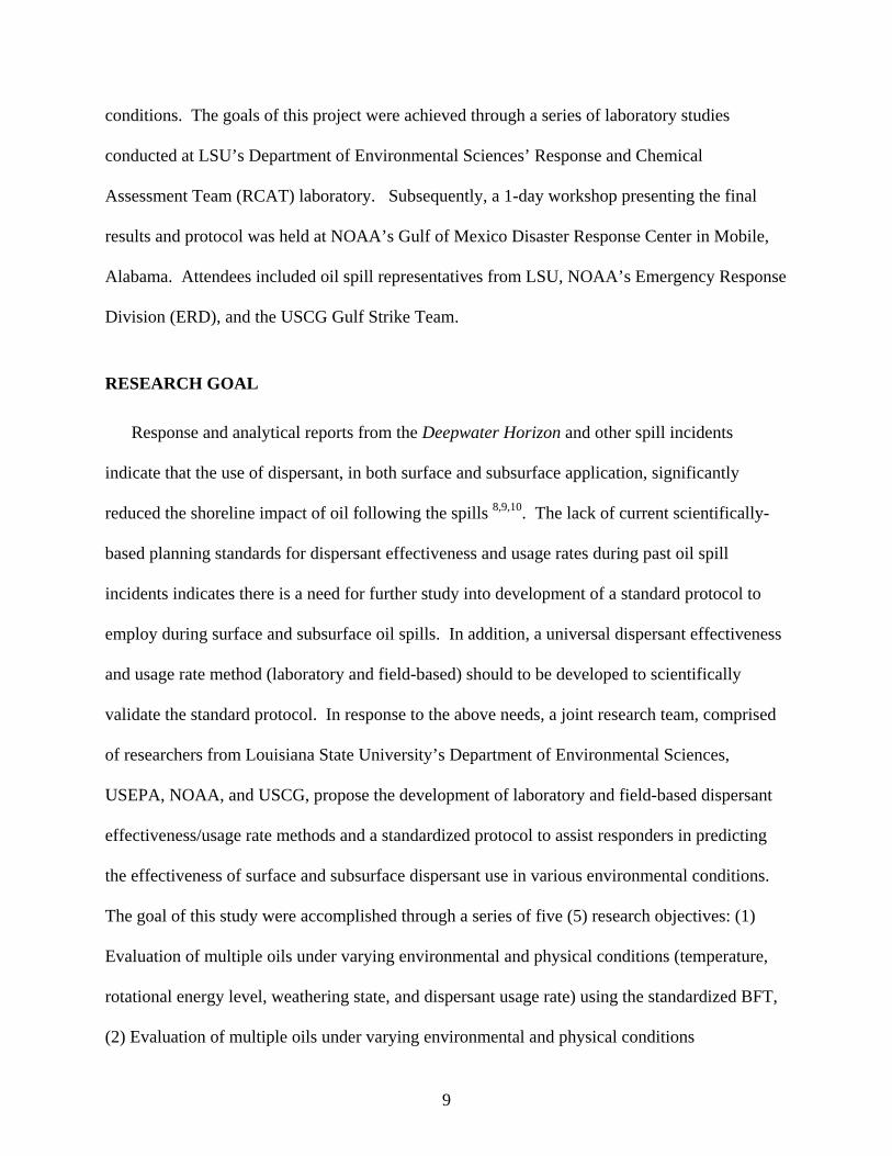
Viscosity API Density (g/ml) at Density (g/ml) at % Aromatics at
Crude Oil Name (cP) at Gravity 23°C and 0% 23°C and 10% 0% Evaporation
15°C Weathering Weathering
South Louisiana Crude
7.1 37.1 0.886 0.944 16.9
North Slope Crude 18 29.8 0.915 0.957 32.0
Hondo Crude 735 19.6 0.987 1.02 31.0
Measured Measured
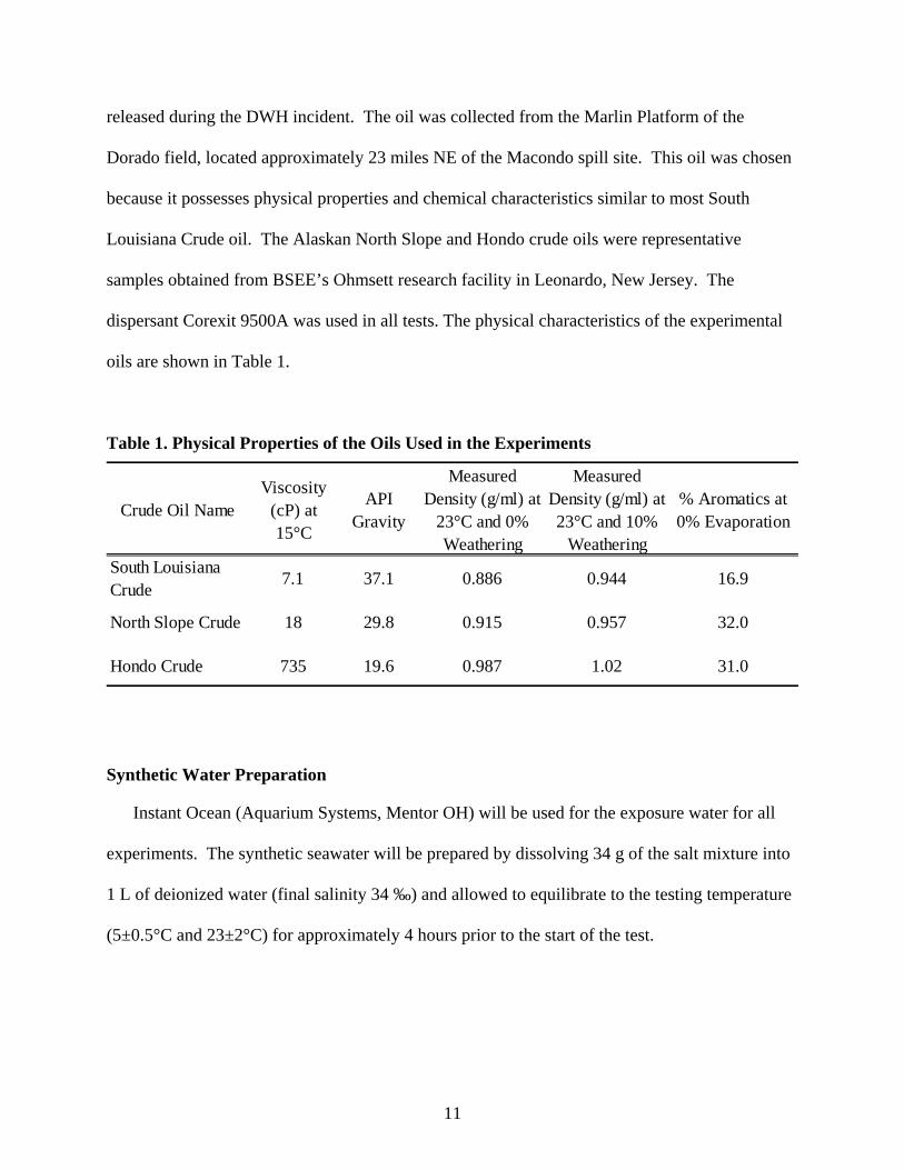
released during the DWH incident. The oil was collected from the Marlin Platform of the
Dorado field, located approximately 23 miles NE of the Macondo spill site. This oil was chosen
because it possesses physical properties and chemical characteristics similar to most South
Louisiana Crude oil. The Alaskan North Slope and Hondo crude oils were representative
samples obtained from BSEE’s Ohmsett research facility in Leonardo, New Jersey. The
dispersant Corexit 9500A was used in all tests. The physical characteristics of the experimental
oils are shown in Table 1.
Table 1. Physical Properties of the Oils Used in the Experiments
Synthetic Water Preparation
Instant Ocean (Aquarium Systems, Mentor OH) will be used for the exposure water for all
experiments. The synthetic seawater will be prepared by dissolving 34 g of the salt mixture into
1 L of deionized water (final salinity 34 ‰) and allowed to equilibrate to the testing temperature
(5±0.5°C and 23±2°C) for approximately 4 hours prior to the start of the test.
11

Analytical Instrumentation
As part of this project, our research team developed and validated analytical methods and
protocols designed for real-time dispersibility determination of crude oils following surface and
deep sea spill incidents. The dispersibility of simulated field oil samples were determined using a
laboratory-based spectrofluorometer system and field-portable turbidity and fluorescence probe
units. The spectrofluorometer system used was a Horiba Aqualog® spectrofluorometer capable
of simultaneously measuring fluorescence and absorbance with matching optical bandpass
resolution. The turbidity meter used was a Hach® model 2100P Portable Turbidimeter and meets
the design criteria specified by the United States Environmental Protection Agency (USEPA) for
water quality measurements using method 180.1. The field fluorescence probe used was a Turner
Designs Cyclops-7™ Submersible Sensor, the same probe integrated into the Turner Designs C3
submersible probe for use in NOAA’s SMART protocol. The Cyclops-7 probe has a dynamic
detection range of 0-25 ppm of dispersed crude oil in water. Analytical instrumentation used
during this project are shown in Figure 1.
Preparation of Crude Oil Standards
A stock standard oil solution of each crude oil- Corexit 9500 dispersant in dichloromethane
(DCM) was prepared by adding 80 μl of the dispersant to a 2.0 ml aliquot of oil, and then
adjusted to a final volume of 20 ml with DCM. A six-point calibration oil calibration curve was
constructed by adding a specific volume of the stock standard oil solution to a 125-ml seperatory
funnel containing a 30 ml aliquot of artificial seawater. Liquid/liquid extractions of the spiked
water samples were then performed three times using a 5 ml aliquot of DCM for each extraction.
The extracts were collected in a 25-ml graduated cylinder and the final volume adjusted to 20 ml
with DCM. The 20 ml sample extract was transferred to a 40-ml vial with a Teflon-lined
12

enclosure. Approximately 1-2 g of anhydrous sodium sulfate was added to the vial to remove
water within the DCM extract. The final extract volume was stored at 5°C until time of analysis.
Oil Extraction and Analysis
Pesticide-grade dichloromethane (DCM) was used to extract oil-water samples from the
baffled flask apparatus. A Brinkmann Eppendorf pipettor was used to dispense the required
amount of oil and dispersant into the experimental flasks. Dispersed oil was measured with a
Horiba Aqualog Spectrofluorometer capable of simultaneously measuring UV-VIS absorbance at
340, 370, and 400 nm and measuring fluorescence excitation-emission matrices. UV-VIS
absorbance measurements were originally used with the SFT protocol and later adopted into the
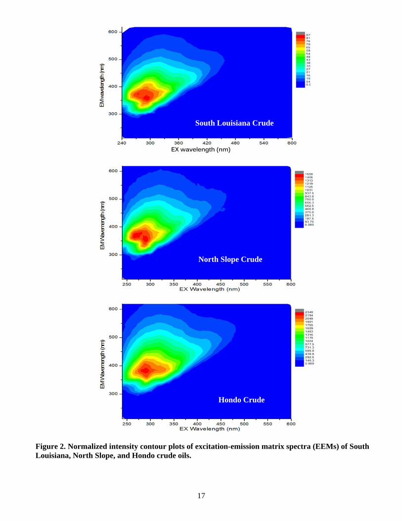
BFT protocol. Fluorescence excitation/emission analysis was performed on the select oils to
determine their maximum peak excitation/emission wavelengths. Excitation-emission matrix
spectroscopy (EEMS) was utilized to characterize the individual crude oils and determine their
maximum excitation and emission wavelengths. The maximum excitation and emission
wavelength for South Louisiana and North Slope crude oil were 290 nm and 360 nm,
respectively. The maximum excitation and emission wavelength for Hondo crude oil was 290 nm
and 380 nm, respectively. The fluorescence analysis allowed investigators to compare and
correlate BFT results with pressure vessel and field BFT results. Standard transmission-matched
quartz 10-mm path length rectangular cells with PFTE covers were used. The excitation-
emission matrix spectroscopy contour plots for South Louisiana, North Slope, and Hondo crude
oils are displayed in Figure 2.
13

A
Figure 1. Photographs of Aqualog spectrofluorometer (top), Turner Designs Cyclops-7 probe (mid), and Hach portable turbidimeter (bottom).
14

Analysis of Sample Extracts
Following the protocol used by the BFT, investigators recorded the absorbance at three
discreet wavelengths of 340, 370, and 400 nm. The area under the absorbance vs. wavelength
curve was calculated by applying the trapezoidal rule according to the following equation:
Area Count = (Abs340 + Abs370) x 30 + (Abs370 + Abs400) x 30 2 2
This area count is used to calculate the Total Oil Dispersed and then the percentage of Oil
Dispersed (%OD) based on the ratio of Oil Dispersed in the test system to the total oil added to
the flask, as follows:
Total Oil Dispersed (g) = Area × VDCM × Vtw
Calib. Curve Slope Vew
where V DCM is the volume of DCM extract, Vtw the total volume of seawater in the baffled flask,
and Vew is the total volume of seawater extracted, and
%OD = 100 × Total Oil Dispersed poil × Voil
where ρ oil is the density of the specific test oil, g/L and Voil is the volume (L) of oil added to test
flask (100 μL ). The dispersion effectiveness value that is reported is the lower 95% confidence
level of the five (5) independent replicates.
15

The following equation summarizes the calculation of the DELCL95:
DELCL95 = mean %OD – tn-1, 1-α( s/n-2 )
where mean %OD is the mean dispersion effectiveness of the n = 5 replicates, s the standard
deviation, and tn−1,1−α = 100 × (1 − α)th percentile from the t-distribution with n − 1 degrees of
freedom.
For five (5) replicates, tn-1,1-α=2.132, where α = 0.05. We performed the same calculations for the
physically dispersed oil (absence of added dispersant) for comparison purposes. An additional
set of dispersion effectiveness values were generated using fluorescence areas. This data set was
used to determine if the fluorescence analysis is more sensitive and accurate when compared to
the UV-VIS method and to correlate dispersant effectiveness values with results from the
pressure vessel and field BFT.
Statistical Analysis
Prior to conducting the statistical comparisons, the replicates within a given treatment were
subjected to the Grubb’s Test (or Maximum Normal Residual test) (Grubbs, 1950) for outliers,
and if an outlier is detected (p < 0.05), an additional replicate was run and analyzed to obtain the
required number of replicates. In addition to calculating the DELCL95 for each task, multiple
factorial analysis of variance (ANOVA) were performed to determine if there is a mean
difference between treatments and identify interactions between the various environmental and
physical conditions. Statistical analysis was performed using IBM SPSS Statistical software.
16
EX wavelength (nm)
South Louisiana Crude
North Slope Crude
Hondo Crude
Figure 2. Normalized intensity contour plots of excitation-emission matrix spectra (EEMs) of South Louisiana, North Slope, and Hondo crude oils.
17

Task #1: 150-ml Baffled Flask Test Study
A series of bench-scale laboratory studies were performed to determine dispersant efficiency
and usage rates for various environmental conditions within a baffled-flask microcosm following
addition of Corexit 9500 to select crude oils. The objective of this study was to compare
analytical methods (Fluorescence vs. UV-Vis) so as to determine which method is best suited for
performing oil recovery analyzes for the standardized baffled flask tests. Five (5) individual
replicate tests for each oil were used in the protocol (5 replicates × 2 temperatures × 4 DORs × 2
mixing energies × 3 oils × 2 weathering states) for a total of 480 tests. In addition, the
instrument calibration curves required a total of 15-18 extractions (5-6 calib. points × 3 oils),
plus a continuing calibration standard and method blank were extracted prior to the daily analysis
of water samples on the spectrofluorometer. The three oils (SLC, ANC, and HC) were evaluated
using the following factors: temperature (5°C and 23°C), DOR (0, 1:20, 1:50, and 1:100), mixing
energy (150 rpm and 200 rpm), and weathering state (fresh and 10% weathered). Corexit 9500A
was used throughout the BFT procedure and the salinity was maintained at 34 ‰. For the tests
performed at 5°C, the shaker unit was housed in a large volume refrigerator and maintained at
5°C±1. All necessary tubing and wiring was plumbed through an insulated port located on the
refrigerator side wall. The shaker unit and pressure vessel apparatus was located on top of
laboratory bench and maintained at 23°C±1 for tests performed at ambient temperature.
The tests used a 150-ml screw-cap trypsinizing flask that has been modified with the addition
of a glass stopcock near the bottom so that a subsurface water sample can be removed without
disturbing the surface oil layer. A 120 ml volume of synthetic water was added, followed by a
100 μl volume of oil and an appropriate volume of Corexit 9500A. The flask was placed on an
orbital shaker to receive low (non-breaking waves) and moderate (breaking waves) turbulent
18

mixing at 150 and 200 rpm, respectively, for 10 ± 0.25 min. The shaker table has a speed control
unit with variable speed (40–400 rpm) and an orbital diameter of approximately 0.75 in. (1.9 cm)
and is used to impart turbulence to solutions in the test flasks. The 150 and 200 mixing rates are
equivalent to an energy dissipation rates of 0.0155 m2/s3 and 0.163 m2/s3, respectively. The
rotational speed accuracy was maintained within ±10%. The contents of the flasks were allowed
to settle for 10 ± 0.25 min to allow non-dispersed oil to return to the water surface before
removing the subsurface water sample. Each replicate was run individually by the same analyst
so that identical test conditions can be maintained for each replicate. A 30 ml volume of
synthetic seawater was collected from each test and placed in a 150-ml seperatory funnel.
Liquid/liquid solvent extraction of the sample was performed three (3) times with 5 ml of DCM
for each extraction. The extracts were collected in a 25-ml graduated cylinder and the final
volume adjusted to 20 ml with DCM. The 20 ml sample extract was transferred to a 40-ml vial
with a Teflon-lined enclosure. Approximately 1-2 g of anhydrous sodium sulfate (drying agent)
was added to each vial to remove water within the DCM extract. The final extract vials were
stored at 5°C until time of analysis. The oil concentration in the DCM was measured by the
Aqualog benchtop spectrofluorometer, simultaneously measuring UV-VIS absorbance and
fluorescence excitation/emission wavelengths. Absorbance was recorded at 340, 370, and 400
nm for determination of UV-Vis absorbance for all crude oils. Oils concentrations (UV-Vis)
were calculated using the trapezoidal rule equation and 5-point UV-Vis standard calibration
curve (Figure A2). South Louisiana and North Slope crude oil fluorescence concentrations were
determined using an excitation wavelength of 290 nm and an emission wavelength of 360 nm.
Hondo crude oil fluorescence concentration was determined using an excitation wavelength of
19

290 nm and an emission wavelength of 390 nm. Oil concentrations were calculated using the 5
point fluorescence standard calibration curve for the individual oils (Figure A1).
Results & Discussion: 150-ml Baffled Flask Tests
The results for the experimental design are displayed in Figs. 3-8, which show the percent
effectiveness from the analytical methods “fluorescence” and “UV-Vis” at various flask speeds,
temperatures, weathering state, and DOR for all three oils. To better understand the significance
of the analytical results, statistical analyses of the experimental data were performed individually
for the three oils. The results of the design experiments were analyzed using a factorial analysis
of variance (ANOVA) at α =0.05 to determine which factors affect percent effectiveness. A
significant interaction means that the effect of one independent variable varies at differing levels
of another independent variable. The condition for significance was determined by statistical
analysis was that the p–value should be less than 0.05 for a factor to be significant. Although this
experiment was designed to determine if a significant difference exist between the two analytical
methods, interactions between the other environmental factors (e.g. temperature, weathering,
energy, and DOR) were examined.
The results showed that all four factors significantly affected the dispersant effectiveness in
SLC (p < 0.005). Figs. 3 and 4 clearly illustrate that all four factors (temperature, weathering,
energy, and DOR) produced significant change in the percent effectiveness values, thus, all these
factors were deemed significant. Results from the statistical analysis indicated there was no
significant difference between the two analytical methods (p = 0.325). There was no significant
two-way interaction between the method factor and the temperature, weathering, energy, and
DOR factors (p > 0.572). For NSC, all four factors (temperature, weathering, energy, and DOR)
were found to significantly affect the dispersant effectiveness (p < 0.005). Figs. 5 and 6 show
20
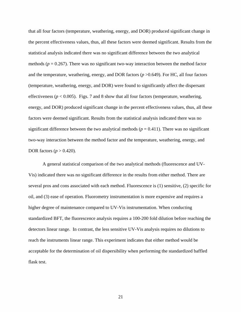
that all four factors (temperature, weathering, energy, and DOR) produced significant change in
the percent effectiveness values, thus, all these factors were deemed significant. Results from the
statistical analysis indicated there was no significant difference between the two analytical
methods (p = 0.267). There was no significant two-way interaction between the method factor
and the temperature, weathering, energy, and DOR factors (p >0.649). For HC, all four factors
(temperature, weathering, energy, and DOR) were found to significantly affect the dispersant
effectiveness (p < 0.005). Figs. 7 and 8 show that all four factors (temperature, weathering,
energy, and DOR) produced significant change in the percent effectiveness values, thus, all these
factors were deemed significant. Results from the statistical analysis indicated there was no
significant difference between the two analytical methods (p = 0.411). There was no significant
two-way interaction between the method factor and the temperature, weathering, energy, and
DOR factors (p > 0.420).
A general statistical comparison of the two analytical methods (fluorescence and UV-
Vis) indicated there was no significant difference in the results from either method. There are
several pros and cons associated with each method. Fluorescence is (1) sensitive, (2) specific for
oil, and (3) ease of operation. Fluorometry instrumentation is more expensive and requires a
higher degree of maintenance compared to UV-Vis instrumentation. When conducting
standardized BFT, the fluorescence analysis requires a 100-200 fold dilution before reaching the
detectors linear range. In contrast, the less sensitive UV-Vis analysis requires no dilutions to
reach the instruments linear range. This experiment indicates that either method would be
acceptable for the determination of oil dispersibility when performing the standardized baffled
flask test.
21
100 100 A Control
1:20 DOR B Control
1:20 DOR 1:50 DOR 1:50 DOR
80 1:100 DOR 80 1:100 DOR
% E
ffect
iven
ess
% E
ffect
iven
ess
60
40
% E
ffect
iven
ess
% E
ffect
iven
ess
60
40
20 20
0 0 UV Visible Fluorescence UV Visible Fluorescence
100 100 Control Control C D1:20 DOR 1:20 DOR 1:50 DOR 1:50 DOR 1:100 DOR 80 80 1:100 DOR
60
40
60
40
20 20
0 0 UV Visible Fluorescence UV Visible Fluorescence
Figure 3. Average percent effectiveness for South Louisiana crude baffled flask study at 5°C with 150 rpm and 0% weathered (A), 150 rpm and 10% weathered (B), 200 rpm and 0% weathered (C), and 200 rpm and 10% weathered (D).
22

40
60
40
60
100 100 Control BA Control 1:20 DOR 1:20 DOR 1:50 DOR 1:50 DOR 80 801:100 DOR 1:100 DOR
% E
ffect
iven
ess
% E
ffect
iven
ess
% E
ffect
iven
ess
% E
ffect
iven
ess
60
40
2020
00 UV Visible Fluorescence UV Visible Fluorescence
100 100 Control Control C D1:20 DOR 1:20 DOR 1:50 DOR 1:50 DOR 1:100 DOR 80 80 1:100 DOR
60
40
20 20
0 0 UV Visible Fluorescence UV Visible Fluorescence
Figure 4. Average percent effectiveness for South Louisiana crude baffled flask study at 23°C with 150 rpm and 0% weathered (A), 150 rpm and 10% weathered (B), 200 rpm and 0% weathered (C), and 200 rpm and 10% weathered (D).
23

100 100 Control B Control A 1:20 DOR 1:20 DOR 1:50 DOR 1:50 DOR
80 801:100 DOR 1:100 DOR
% E
ffect
iven
ess
% E
ffect
iven
ess
60
40
% E
ffect
iven
ess
% E
ffect
iven
ess
60
40
20 20
0 0 UV Visible Fluorescence UV Visible Fluorescence
100 100 Control Control C D 1:20 DOR 1:20 DOR 1:50 DOR
80 1:50 DOR
1:100 DOR 801:100 DOR
60
40
60
40
20 20
0 0 UV Visible Fluorescence UV Visible Fluorescence
Figure 5. Average percent effectiveness for North Slope crude baffled flask study at 5°C with 150 rpm and 0% weathered (A), 150 rpm and 10% weathered (B), 200 rpm and 0% weathered (C), and 200 rpm and 10% weathered (D) .
24

100 100 Control Control A B 1:20 DOR 1:20 DOR 1:50 DOR 1:50 DOR
80 80 1:100 DOR 1:100 DOR
% E
ffect
iven
ess
% E
ffect
iven
ess
60
40
20
% E
ffect
iven
ess
% E
ffect
iven
ess
60
40
20
0 UV Visible Fluorescence UV Visible Fluorescence
0
100 100 Control Control DC 1:20 DOR 1:20 DOR 1:50 DOR 1:50 DOR 1:100 DOR 1:100 DOR 80 80
60
40
60
40
20 20
0 0 UV Visible Fluorescence UV Visible Fluorescence
Figure 6. Average percent effectiveness for North Slope crude baffled flask study at 23°C with 150 rpm and 0% weathered (A), 150 rpm and 10% weathered (B), 200 rpm and 0% weathered (C), and 200 rpm and 10% weathered (D).
25

50 50
A Control B Control 1:20 DOR 1:20 DOR
40 1:50 DOR 1:100 DOR
40 1:50 DOR 1:100 DOR
% E
ffect
iven
ess
% E
ffect
iven
ess
30
20
% E
ffect
iven
ess
% E
ffect
iven
ess
30
20
10 10
0 0 UV Visible Fluorescence UV Visible Fluorescence
50 50 DC Control Control
1:20 DOR 1:20 DOR 1:50 DOR 1:50 DOR 40 401:100 DOR 1:100 DOR
30
20
30
20
10 10
0 0 UV Visible Fluorescence UV Visible Fluorescence
Figure 7. Average percent effectiveness for Hondo crude baffled flask study at 5°C with 150 rpm and 0% weathered (A), 150 rpm and 10% weathered (B), 200 rpm and 0% weathered (C), and 200 rpm and 10% weathered (D).
26

50 50 Control Control A B 1:20 DOR 1:20 DOR 1:50 DOR 1:50 DOR
40 40 1:100 DOR 1:100 DOR
% E
ffect
iven
ess
% E
ffect
iven
ess
30
20
10
% E
ffect
iven
ess
% E
ffect
iven
ess
30
20
10
0 UV Visible Fluorescence UV Visible Fluorescence
0
50 50 C Control Control D
1:20 DOR 1:20 DOR 1:50 DOR 1:50 DOR 40 401:100 DOR 1:100 DOR
30
20
30
20
10 10
0 0 UV Visible Fluorescence UV Visible Fluorescence
Figure 8. Average percent effectiveness for Hondo crude baffled flask study at 23°C with 150 rpm and 0% weathered (A), 150 rpm and 10% weathered (B), 200 rpm and 0% weathered (C), and 200 rpm and 10% weathered (D).
27

Task #2: Pressure Vessel Study
A series of high-pressure static vessel laboratory studies were performed to determine
dispersant effectiveness and usage rates for subsea dispersant use in various types of
environmental conditions within a 1-L stainless steel pressure vessel with the addition of Corexit
9500 to three select crude oils. The study was designed to simulate the release of oil from subsea
releases at various depths and pressure. The objective of this research was to develop a set of
empirical data on three oils and two pressures, by studying the variation in the dispersant
effectiveness caused by changes in temperature, oil weathering, and dispersant to oil ratio. The
pressure apparatus was developed and manufactured through a previous grant from BSEE. The
main vessel (Figures 9 and 10) is manufactured by Applied Separations, Inc. (Allentown, PA)
and designed to withstand pressures up to 10,000 psi. Accessories included with the vessel are a
high-pressure liquid pump with an integrated microprocessor logging unit, a temperature and
pressure probe, a high-pressure stirrer unit, and multiple sampling ports. The high-pressure
stirrer operated at a rotational speed of 400 rpm. The sampling port was connected to a ¼”
sampling tube which collected samples from the centerline of the vessel and approximately three
(3) inches below the paddle stirrer. The high-pressure liquid pumping system was designed to
maintain a constant pressure level throughout the experiments, allowing researchers to sample
the vessel contents with no significant drop in pressure.
The three oils (SLC, ANC, and HC) were tested within the pressure vessel at various
temperatures (5°C and 23°C) and pressures (200 psi, and 2000 psi) using control crude oils (no
dispersant) and chemically-dispersed (DOR=1:20, 1:50, and 1:100) crude oil treatments. Corexit
9500A was used throughout the pressure vessel study and the salinity was maintained at 32 ‰.
28

WATER PUMP
Stirrer
WATER IN WATER OUT
SHUT-OFF VALVE
AIR DRAIN LINE
SHUT-OFF VALVE
SAMPLE LINE
COLLECTION VIAL
MIXING BLADE
PRESSURE CELL
Figure 9. Experimental design for the determination of dispersant effectiveness in water at elevated pressures.
Three (3) individual replicate tests for each oils were used in the protocol (3 replicates × 2
temperatures × 4 DORs × 3 oils × 2 weathering states) for a total of 144 tests. Oil concentration
in water was determined using the fluorescence analytical method detailed in the Task #1 study.
In addition, a continuing calibration standard and method blank were extracted prior to the daily
analysis of water samples on the spectrofluorometer. Each replicate was run individually by the
same analyst so identical test conditions can be maintained for each replicate.
29

Figure 10. Photographs of high-pressure vessel and pumping system.
30

A 1 ml volume of oil or oil/dispersant mixture was injected through a 1/8” injection port into
the 1-L vessel filled with synthetic seawater and allowed to equilibrate to the designated test
temperature. For the tests perform at 5°C, the pressure vessel apparatus was housed in a large
volume refrigerator and maintained at 5°C±1. All necessary tubing and wiring was plumbed
through an insulated port located on the refrigerator side wall. The stirrer unit and pressure
vessel apparatus was located on a laboratory bench and maintained at 23°C±1 for tests performed
at ambient temperature. The stirrer unit was activated and the vessel slowly pressurized to the
designated test pressure and allowed to equilibrate for approximately 15 minutes. The contents of
sampling tube were pre-drained to remove any water trapped within the tube. A 30 ml volume of
synthetic seawater was collected from each test and placed in a 150-ml seperatory funnel.
Liquid/liquid solvent extraction of the sample was performed three (3) times with 5 ml of DCM
for each extraction. The extracts were collected in a 25-ml graduated cylinder and the final
volume adjusted to 20 ml with DCM. The 20 ml sample extract was transferred to a 40-ml vial
with a Teflon-lined enclosure. Approximately 1-2 g of anhydrous sodium sulfate (drying agent)
was added to each vial to remove water within the DCM extract. The final extract vials were
stored at 5°C until time of analysis. South Louisiana and North Slope crude oil fluorescence
concentrations were determined by the Aqualog benchtop spectrofluorometer using an excitation
wavelength of 290 nm and an emission wavelength of 360 nm. Hondo crude oil fluorescence
concentration was determined using an excitation wavelength of 290 nm and an emission
wavelength of 390 nm. Oil concentrations were calculated using the 5-point fluorescence
standard calibration curve for the individual oils (Figure A1).
31
Results & Discussion: Pressure Vessel Study
The results for the experimental design are displayed in Fig. 11, which show the percent
effectiveness at various pressures, temperatures, and DOR for all three oils. The averaged results
for the high-pressure vessel experiments are displayed in Tables A9 and A10. To better
understand the significance of the analytical results, statistical analyses of the experimental data
were performed individually for the three oils. The results of the design experiments were
analyzed using a factorial analysis of variance (ANOVA) at α =0.05 to determine which factors
affect percent effectiveness. A significant interaction means that the effect of one independent
variable varies at differing levels of another independent variable. The condition for significance
was determined by statistical analysis was that the p–value should be less than 0.05 for a factor
to be significant. Although this experiment was designed to determine if a significant difference
exist between the two pressures, interactions between the other environmental factors (e.g.
temperature, energy, and DOR) were examined.
The results showed that two factors (temperature and DOR) significantly affected the
dispersant effectiveness in SLC (p < 0.005). Fig. 11 illustrates that two of the three factors
(temperature, pressure, and DOR) produced significant change in the percent effectiveness
values, thus, temperature and DOR were deemed significant. Results from the statistical analysis
indicated there was no significant effect from changes in pressure (p = 0.235). The statistical
analysis determined there was a significant two-way interaction between temperature and DOR
(p = 0.001), but no two-way significant interaction with the pressure vs. temperature and
pressure vs. DOR interactions (p = 0.163 and 0.307, respectively). A Tukey Post Hoc test
indicated there was no significant difference between the DOR 1:20 and 1:50 treatments (p =
0.065). For NSC, two of the three factors (temperature and DOR) were found to significantly
32
affect the dispersant effectiveness (p < 0.005). Fig. 11 shows that two factors (temperature and
DOR) produced significant change in the percent effectiveness values, thus, all these factors
were deemed significant. Results from the statistical analysis indicated there was no significant
effect from changes in pressure (p = 0.864). The statistical analysis determined there was a
significant two-way interaction between temperature and DOR (p = 0.007), but no two-way
significant interaction with the pressure vs. temperature and pressure vs. DOR interactions (p =
0.891 and 0.886, respectively). A Tukey Post Hoc test indicated there was no significant
difference between the control and three dispersant treatments (p < 0.018). For HC, two of the
three factors (temperature and DOR) were found to significantly affect the dispersant
effectiveness (p < 0.005). Fig. 11 shows that two factors (temperature and DOR) produced
significant change in the percent effectiveness values, thus, all these factors were deemed
significant. Results from the statistical analysis indicated there was no significant effect from
changes in pressure (p = 0.323). The statistical analysis determined there was no significant two-
way interaction between pressure vs. temperature, pressure vs. DOR, and temperature vs. DOR
(p = 0.897, p = 0.929, and p = 0.430, respectively). A Tukey Post Hoc test indicated there was no
significant difference between the control and three dispersant treatments (p < 0.004).
Dispersant effectiveness of oil by chemical dispersants is driven by a range of physical and
environmental variables and includes: type of oil, degree of weathering, type of dispersant used,
mixing energy, and sea water temperature. One of the most important physical properties of oil is
its viscosity, which is a critical parameter influencing the chemical dispersion of oil at various
sea temperatures. A number of correlations for the estimation of oil viscosity based on measured
fluid properties have been formulated, but all indicate viscosity is inversely proportional to
temperature.
33
Figure 11 shows that as temperature increases from 5°C to 23°C, dispersion efficacy
increased 15.8%, 22.0%, and 12.4% for South Louisiana, North Slope, and Hondo crude oils,
respectively. This trend in dispersant effectiveness with an increase in the sea water temperature
has been observed in previous dispersant studies designed to investigate the effects of
temperature on various oil and dispersant properties such as density, viscosity, and surface
tension 11. These studies have shown there is a clear inverse correlation between dispersant
effectiveness and temperature at the experiment temperature range (5°C to 23°C).
The effect of DOR on dispersant effectiveness is observed by examining Figure 11.
Generally, as the DOR in the oil increases, dispersant effectiveness increases. For example, with
unweathered SLC with DOR = 1:20 at 2000 psi and 5°C, the average dispersant effectiveness
was 48.9%, whereas the DOR = 1:50 and 1:100 averaged 45.6% and 36.8% at the same
conditions, respectively. Similarly, for unweathered NSC with DOR = 1:20 at 2000 psi and 5°C,
the average dispersant effectiveness was 44.7%, whereas the DOR = 1:50 and 1:100 averaged
38.5% and 36.2% at the same conditions, respectively. Again, for unweathered HC with DOR =
1:20 at 2000 psi and 5°C, the average dispersant effectiveness was 13.9%, whereas the DOR =
1:50 and 1:100 averaged 12.4% and 8.37% at the same conditions, respectively.
Figure 11 shows the results obtained for oil and oil + dispersant combinations at 32 ppt
salinity at various pressures. From this figure, it is seen that for a given oil at a specified
temperature or DOR, as the pressure of the system increases, no significant change in dispersant
effectiveness was observed. For example, for unweathered SLC (5°C and DOR = 1:20) at 200
psi, the average dispersant effectiveness was 48.3%, whereas at 2000 psi the average
effectiveness was 48.9%. In the case of NSC, unweathered oil (5°C and DOR = 1:20) at 200 psi,
the average dispersant effectiveness was 45.1%, whereas at 2000 psi the average effectiveness
34
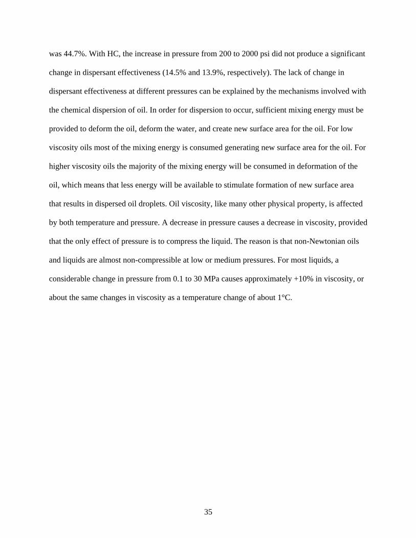
was 44.7%. With HC, the increase in pressure from 200 to 2000 psi did not produce a significant
change in dispersant effectiveness (14.5% and 13.9%, respectively). The lack of change in
dispersant effectiveness at different pressures can be explained by the mechanisms involved with
the chemical dispersion of oil. In order for dispersion to occur, sufficient mixing energy must be
provided to deform the oil, deform the water, and create new surface area for the oil. For low
viscosity oils most of the mixing energy is consumed generating new surface area for the oil. For
higher viscosity oils the majority of the mixing energy will be consumed in deformation of the
oil, which means that less energy will be available to stimulate formation of new surface area
that results in dispersed oil droplets. Oil viscosity, like many other physical property, is affected
by both temperature and pressure. A decrease in pressure causes a decrease in viscosity, provided
that the only effect of pressure is to compress the liquid. The reason is that non-Newtonian oils
and liquids are almost non-compressible at low or medium pressures. For most liquids, a
considerable change in pressure from 0.1 to 30 MPa causes approximately +10% in viscosity, or
about the same changes in viscosity as a temperature change of about 1°C.
35
% E
ffect
iven
ess
% E
ffect
iven
ess
70 A Control
60 1:20 DOR 1:50 DOR 1:100 DOR
50
40
30
20
10
0 SLC NSC HC
70 C Control
60 1:20 DOR 1:50 DOR 1:100 DOR
50
40
30
20
10
0 SLC NSC HC
Figure 11. Average percent effectiveness for South Louisiana, North Slope, and Hondo crude baffled flask study at 23°C and 200 psi (A), 23°C and 2000 psi (B), 5°C and 200 psi (C), and 5°C and 2000 psi (D).
36

Task #3: 1-L Baffled Flask Test Study
A series of large bench-scale laboratory studies were performed to determine dispersant
efficiency and usage rates for various environmental conditions using a 1-L baffled-flask to
evaluate three specific oils. The objective of this study was to develop a standardized method
and protocol to estimate the real-time effectiveness of dispersants using common laboratory
glassware and an in-situ fluorescence probe. The field-portable testing “kit” will allow oil spill
responders to determine if a specific oil is “dispersable” prior to actual full-scale operations. In
addition to testing the fluorescence probe, a portable turbidimeter was utilized for comparison to
the laboratory-based and portable fluorescence probe dispersant effectiveness results. Three (3)
individual replicate tests for each oil were used in the protocol (3 replicates × 2 temperatures × 4
DORs × 2 mixing energies × 3 oils × 2 weathering states) for a total of 288 tests. In addition, a
continuing calibration standard and method blank were extracted prior to the daily analysis of
water samples on the spectrofluorometer. The three oils (SLC, ANC, and HC) were evaluated
using the following factors: temperature (5°C and 23°C), DOR (0, 1:20, 1:50, and 1:100), mixing
energy (150 rpm and 200 rpm), and weathering state (fresh and 15% weathered). Corexit 9500A
was used throughout the 1-L BFT procedure and the salinity was maintained at 32 ‰. For the
tests performed at 5°C, the shaker unit was housed in a large volume refrigerator and maintained
at 5°C±1. All necessary tubing and wiring were plumbed through an insulated port located on
the refrigerator side wall. The shaker unit and pressure vessel apparatus were located on a
laboratory bench and maintained at 23°C±1 for tests performed at ambient temperature.
The 1-L BFT test utilizes a 1-L open trypsinizing flask that has been modified with the
addition of a glass stopcock near the bottom so that a subsurface water sample can be removed
without disturbing the surface oil layer. A 600 ml volume of synthetic water is added, followed
37

by the addition of a 500 μl aliquot of oil and an appropriate volume of Corexit 9500A to achieve
the desired DOR. The oil to water ratio used in the 1-L BFT is equivalent to the oil to water ratio
employed in the 150-ml standardized BFT. The cylindrical stainless steel probe is 6” in length
and 1” in diameter. This device is the same fluorescence probe that is currently installed on the
larger Turner Designs C3 fluorometer unit used by the USCG for in situ monitor of oil spills
during full-scale dispersant operations. The flask is placed on a small digital orbital shaker (11”
× 13”) to receive low (non-breaking waves) and moderate (breaking waves) turbulent mixing at
150 and 200 rpm, respectively, for 10 ± 0.25 min. The shaker table has a speed control unit with
variable speed (40–400 rpm) and an orbital diameter of approximately 0.75 in. (1.9 cm) is used
to impart turbulence to solutions in the test flasks. The rotational speed accuracy should be
within ±10%. The contents of the flasks are allowed to settle for 10 ± 0.25 min to allow non-
dispersed oil to return to the water surface before removing the subsurface water sample. Prior
to collecting sample from the 1-L baffled flask, a 10-15 ml aliquot of water is wasted from the
stopcock drain in order to remove any residual oil trapped within the drain stem. Each replicate
is run individually by the same analyst so that identical test conditions can be maintained for
each replicate.
For the fluorescence probe and turbidity determinations, a 200-ml volume of sample was
slowly drained into a calibrated 300 ml glass jar. The Cyclops-7 probe was inserted into the
samples and held approximately 2” below the water surface. The probe was swirled slowly to
remove any air bubbles trapped beneath the probe tip. The fluorescence probe was activated and
fluorescence measurements were recorded for approximately 30-35 seconds at a scan rate of 1
scan per second. The fluorescence response (mv) was averaged and recorded. The linear
response range for the Cyclops-7 field probe was determined to be 60-1500 mv, 60-500 mv, and
38

60-250 mv for SLC, NSC, and HC, respectively. The baseline response for artificial seawater
averaged 12 mv throughout the experiment. If the sample response exceeded the linear range for
that specific oil, the sample was diluted until the response reached 40-60% of the maximum
linear response for that oil. Field probe and turbidimeter calibration curves were constructed for
each unweathered oil by performing a 1-L BFT at 23°C, DOR = 1:20, and 150 rpm. This
combination of parameters (0% weathering, 23°C, DOR = 1:20, and 150 rpm) was designate as
the baseline condition for predicting percent dispersant effectiveness. These parameters were
chosen because they represented the conditions that are considered optimal for the safe
application of chemical dispersants during field operations. Field probe and turbidimeter
responses were measured at seven (7) levels (undiluted and 2x, 4x, 8x, 16x, 32x, and 64x
dilution) using serial dilutions and corresponding water samples extracted to determine oil
concentration by laboratory-based fluorescence. The percent oil dispersed was determined using
the calculations presented in the analysis of sample extracts section of this document. A 5-point
calibration curve for each oil was then constructed by plotting the percent effectiveness versus
the field probe or turbidimeter response within their respective linear range. The 5-point field
probe and turbidimeter calibration curves with 95% confidence levels for each oil is shown in
Figures A3 and A4, respectively.
The percent dispersant effectiveness for each oil and treatment was determined by the linear
regression equations found in Figure A3. A 10-ml turbidity and 30-ml laboratory fluorescence
analysis subsample was immediately taken from the calibrated 300-ml glass jar. The 10 ml
turbidity sample was collected in a 15-ml vial and immediately measured using a tungsten white
light source and detector spectral peak response between 400nm and 600nm. The linear response
39
range for the turbidimeter was factory calibrated to 0.1-1000 NTU. If the sample response was
greater than the upper limit, a dilution was made until response was within the linear range. The
percent dispersant effectiveness for each oil and treatment was determined by the linear
regression equations found in Figure A4.
For the laboratory-based benchtop fluorescence analysis, a 30 ml volume of synthetic
seawater was collected from each test and placed in a 150-ml seperatory funnel. Liquid/liquid
solvent extraction of the sample was performed three (3) times with 5 ml of DCM for each
extraction. The extracts were collected in a 25-ml graduated cylinder and the final volume
adjusted to 20 ml with DCM. The 20 ml sample extract was transferred to a 40-ml vial with a
Teflon-lined enclosure. Approximately 1-2 g of anhydrous sodium sulfate (drying agent) was
added to each vial to remove water within the DCM extract. The final extract vials were stored
at 5°C until time of analysis. The oil concentration in the DCM was measured by the Aqualog
benchtop spectrofluorometer, simultaneously measuring UV-VIS absorbance and fluorescence
excitation/emission wavelengths. UV-VIS absorbance measurements were not recorded for the
1-L Baffled flask experiment. South Louisiana and North Slope crude oil fluorescence
concentrations were determined using an excitation wavelength of 290 nm and an emission
wavelength of 360 nm. Hondo crude oil fluorescence concentration was determined using an
excitation wavelength of 290 nm and an emission wavelength of 390 nm. Oil concentrations
were calculated using the 5-point fluorescence standard calibration curve for the individual oils
(Figure A1).
40

Results & Discussion: 1-L Baffled Flask Tests
The results for the experimental design are displayed in Figs. 12-17 and tables A11-A22,
which show the percent effectiveness from the analytical devices “laboratory”, “field probe”, and
“turbidimeter” at various flask speeds, temperatures, weathering state, and DOR for all three oils.
To better understand the significance of the analytical results, statistical analyses of the
experimental data were performed individually for the three oils. The results of the design
experiments were analyzed using a factorial analysis of variance (ANOVA) at α =0.05 to
determine which factors affect percent effectiveness. A significant interaction means that the
effect of one independent variable varies at differing levels of another independent variable. The
condition for significance was determined by statistical analysis was that the p–value should be
less than 0.05 for a factor to be significant. This experiment was designed to determine if a
significant difference exist between the three analytical devices, so no interactions between other
environmental factors (e.g. temperature, weathering, energy, and DOR) were examined.
A preliminary ANOVA statistical analysis showed there was an overall significant difference
when comparing the “laboratory”, “field probe”, and “turbidimeter” percent effectiveness results
(p < 0.0005) for all three oils. Tukey post hoc tests showed there was no significance interaction
between the laboratory-based fluorescence and field probe percent effectiveness results for South
Louisiana, North Slope, and Hondo crude oils (p = 0.368, p = 0.743, and p = 0.689,
respectively). The Tukey post hoc tests indicated the overall significant interaction between the
instrument’s responses occurred between the laboratory-based fluorescence and turbidimeter (p <
0.02) and the field probe and turbidimeter (p < 0.002). Due to the significant differences between
the turbidimeter results and the laboratory-based fluorescence results, the investigators
determined turbidity was not a valid parameter for estimating dispersant effectiveness during
41
field operations. A second ANOVA was performed, without the turbidimeter results, to confirm
the correlation between the laboratory-based fluorescence analysis and the field probe analysis.
Again, the ANOVA tests showed there was no significance mean difference between the
laboratory-based fluorescence and field probe percent effectiveness results for South Louisiana,
North Slope, and Hondo crude oils (p = 0.757, p = 0.582, and p = 0.265, respectively).
A statistical comparison of the two analytical instruments (laboratory-based fluorescence and
field probe fluorescence) indicated there was no significant difference in the results from either
instrument. The investigators’ objective for this experiment was to develop an in-situ method for
predicting the percent effectiveness of chemical dispersants in field conditions and be
comparable to laboratory-based fluorescence results. The experiment clearly showed the 1-L
BFT was capable of producing percent effectiveness results comparable to laboratory results. In
order to use the existing oil calibration curves and estimated percent effectiveness equations in
the field, investigators had to formulate a correction factor (CF) to compensate for the different
variables (e.g. water temperature, weathering, and sea state) encountered during actual dispersant
operations. The correction factor was created by normalizing the average percent effectiveness at
the specific oil’s baseline condition (0% weathering, 23°C, DOR = 1:20, and 150 rpm). For
example, the average percent effectiveness for unweathered SLC at 23°C and 200 rpm (breaking
waves) and SLC’s baseline condition were 79.2% and 63.2%, respectively. The CF for
unweathered SLC at 23°C and 200 rpm was calculated by dividing the field condition percent
effectiveness by the baseline condition percent effectiveness (79.2/63.2 = 1.25). The CF for all
oils and field conditions are displayed in Table 2.
42

Table 2. Correction factors for oils and field conditions.
Oil Name Temperature (°C) Weathering (%) Sea Statea Correction Factor (CF)
South Louisiana Crude 5 0 non-breaking 0.844 South Louisiana Crude 5 10 non-breaking 0.626 South Louisiana Crude 5 0 breaking 1.13 South Louisiana Crude 5 10 breaking 1.15
South Louisiana Crudeb 23 0 non-breaking 1.00
South Louisiana Crude 23 10 non-breaking 0.719 South Louisiana Crude 23 0 breaking 1.25 South Louisiana Crude 23 10 breaking 1.13
North Slope Crude 5 0 non-breaking 1.09 North Slope Crude 5 10 non-breaking 0.929 North Slope Crude 5 0 breaking 1.42 North Slope Crude 5 10 breaking 1.28
North Slope Crudeb 23 0 non-breaking 1.00
North Slope Crude 23 10 non-breaking 1.14 North Slope Crude 23 0 breaking 1.49 North Slope Crude 23 10 breaking 1.41
Hondo Crude 5 0 non-breaking 0.965 Hondo Crude 5 10 non-breaking 0.907 Hondo Crude 5 0 breaking 1.11 Hondo Crude 5 10 breaking 0.884
Hondo Crudeb 23 0 non-breaking 1.00
Hondo Crude 23 10 non-breaking 0.956 Hondo Crude 23 0 breaking 1.41 Hondo Crude 23 10 breaking 1.19 a non-breaking (1-4' seas), breaking (4-8' seas) b Baseline condition for estimating % dispersant effectiveness
In the field, a responder would have to collect an oil sample from a vessel, transport the
sample back to a nearby vessel or facility, and perform a 1-L BFT (at baseline conditions) to
determine the percent dispersant effectiveness of Corexit 9500 on that specific oil. The field
probe response would then be inputted into the baseline condition equation and multiplied with
the field CF and dilution factor (DF) to compute the predicted percent effectiveness. The
predicted dispersant effectiveness equations formulated in this study were developed exclusively
43

for South Louisiana, North Slope, and Hondo crude oils. In order to predict the dispersant
effectiveness of other oils, laboratory and field instrument calibration curves and dispersant
effectiveness equations must be determined prior to use. The predicted dispersant effectiveness
equations for South Louisiana, North Slope, and Hondo crude oils are displayed in Table 3.
Table 3. Predicted dispersant effectiveness equation for South Louisiana, North Slope, and Hondo crude oils at baseline conditions
Oil Type 1-L BFT condition Predicted dispersant effectiveness equation
South Louisiana Crude 0% weathering, 23°C, DOR = 1:20, and 150 rpm % Effectiveness = (DF)(CF)(0.0118)(Probe Response)
North Slope Crude 0% weathering, 23°C, DOR = 1:20, and 150 rpm % Effectiveness = (DF)(CF)(0.0364)(Probe Response)
Hondo Crude 0% weathering, 23°C, DOR = 1:20, and 150 rpm % Effectiveness = (DF)(CF)(0.2017)(Probe Response)
For example, a large oil tanker and freighter have collided in the Bering Sea and the tanker has
the potential to sink. The tanker is carrying an unknown amount of North Slope crude oil and the
water temperature is approximately 5°C. The waves are currently non-breaking at 3-4 feet. A
responder would sample the oil and transport it to a nearby response vessel for 1-L baffled flask
testing. At baseline conditions (0% weathering, 23°C, DOR = 1:20, and 150 rpm), the field
probe’s response was 185 mv with an 8-fold dilution. The predicted dispersant effectiveness
would be calculated:
% Effectiveness = (8) (1.09) (0.0364) (185) = 58.7%
To test the predictability of our method and equation, a random group (n=10) of simulated 1-L
BFTs were performed at various environmental conditions (water temperature, mixing energy,
44

and weathering state) for each experimental oil (SLC, NSC, and HC). The observed or predicted
percent effectiveness was measured with the field probe and the actual percent effectiveness was
measured using the liquid-liquid extraction methods and laboratory-based fluorescence analysis.
A linear regression analysis was performed on the results from the laboratory and field
measurements and plotted on a graph. The 95% prediction interval for each oil was then
determined for each oil. Prediction intervals tell you where you can expect to see the next data
point sampled, assuming the data is randomly sampled from a Gaussian distribution. The key
point is that the prediction interval tells you about the distribution of values, not the uncertainty
in determining the population mean. Prediction intervals are always greater than a confidence
interval. The 95% prediction interval for South Louisiana, North Slope, and Hondo crude oil
were ±7.59%, ±6.52%, and ±9.48% dispersant effectiveness, respectively. Using Hondo crude
oil as an example, we can be 95% confident that this range (±9.48%) includes the predicted
percent dispersant effectiveness obtained while using the linear regression equation and percent
effectiveness calculation.
45

% E
ffect
iven
ess
0
20
40
60
80
100 Lab Fluorescence Field Fluorescence Turbidity
A
% E
ffect
iven
ess
0
20
40
60
80
100
Lab Fluorescence Fiels Fluorescence Field Turbidity
B
1:20 1:50 1:100 1:20 1:50 1:100
DOR DOR
% E
ffect
iven
ess
0
20
40
60
80
100 CLab Fluorescence
Field Fluorescence Field Turbidity
% E
ffect
iven
ess
0
20
40
60
80
100 Lab Fluorescence Field Fluorescence Field Turbidity
D
1:20 1:50 1:100 1:20 1:50 1:100
DOR DOR
Figure 12. Average percent effectiveness for South Louisiana crude baffled flask study at 5°C with 150 rpm and 0% weathering (A), 150 rpm and 10% weathering (B), 200 rpm and 0% weathering (C), and 200 rpm and 10% weathering (D).
46
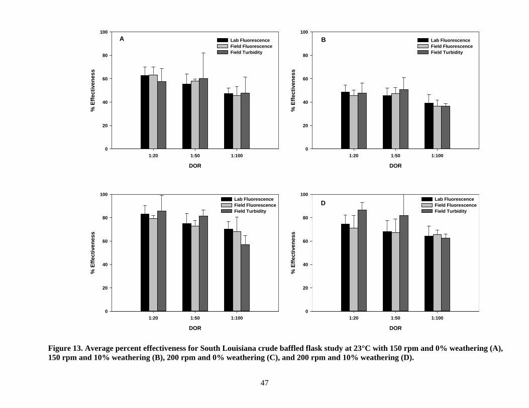
% E
ffect
iven
ess
0
20
40
60
80
100
Lab Fluorescence Field Fluorescence Field Turbidity
A
% E
ffect
iven
ess
0
20
40
60
80
100
Lab Fluorescence Field Fluorescence Field Turbidity
B
1:20 1:50 1:100 1:20 1:50 1:100
DOR DOR
% E
ffect
iven
ess
0
20
40
60
80
100 Lab Fluorescence Field Fluorescence Field Turbidity
% E
ffect
iven
ess
0
20
40
60
80
100 Lab Fluorescence Field Fluorescence Field Turbidity
D
1:20 1:50 1:100 1:20 1:50 1:100
DOR DOR
Figure 13. Average percent effectiveness for South Louisiana crude baffled flask study at 23°C with 150 rpm and 0% weathering (A), 150 rpm and 10% weathering (B), 200 rpm and 0% weathering (C), and 200 rpm and 10% weathering (D).
47

% E
ffect
iven
ess
0
20
40
60
80
100
Lab Fluorescence Field Fluorescence Field Turbidity
A
% E
ffect
iven
ess
0
20
40
60
80
100
Lab Fluorescence Field Fluorescence Field Turbidity
B
1:20 1:50 1:100 1:20 1:50 1:100
DOR DOR
% E
ffect
iven
ess
0
20
40
60
80
100
Lab Fluorescence Field Fluorescence Field Turbidity
C
% E
ffect
iven
ess
0
20
40
60
80
100
Lab Fluorescence Field Fluorescence Field Turbidity
D
1:20 1:50 1:100 1:20 1:50 1:100
DOR DOR
Figure 14. Average percent effectiveness for North Slope crude baffled flask study at 5°C with 150 rpm and 0% weathering (A), 150 rpm and 10% weathering (B), 200 rpm and 0% weathering (C), and 200 rpm and 10% weathering (D).
48

% E
ffect
iven
ess
0
20
40
60
80
100
Lab Fluorescence Field Fluorescence Field Turbidity
A
% E
ffect
iven
ess
0
20
40
60
80
100
Lab Fluorescence Field Fluorescence Field Turbidity
B
1:20 1:50 1:100 1:20 1:50 1:100
DOR DOR
% E
ffect
iven
ess
0
20
40
60
80
100 Lab Fluorescence Field Fluorescence Field Turbidity
C
% E
ffect
iven
ess
0
20
40
60
80
100 Lab Fluorescence Field Fluorescence Field Turbidity
D
1:20 1:50 1:100 1:20 1:50 1:100
DOR DOR
Figure 15. Average percent effectiveness for North Slope crude baffled flask study at 23°C with 150 rpm and 0% weathering (A), 150 rpm and 10% weathering (B), 200 rpm and 0% weathering (C), and 200 rpm and 10% weathering (D).
49

% E
ffect
iven
ess
0
10
20
30
40
50
Lab Fluorescence Field Fluorescence Field Turbidity
A
% E
ffect
iven
ess
0
10
20
30
40
50
Lab Fluorescence Field Fluorescence Field Turbidity
B
1:20 1:50 1:100 1:20 1:50 1:100
DOR DOR
% E
ffect
iven
ess
0
10
20
30
40
50
Lab Fluorescence Field Fluorescence Field Turbidity
C
% E
ffect
iven
ess
0
10
20
30
40
50
Lab Fluorescence Field Fluorescence Field Turbidity
D
1:20 1:50 1:100 1:20 1:50 1:100
DOR DOR
Figure 16. Average percent effectiveness for Hondo crude baffled flask study at 5°C with 150 rpm and 0% weathering (A), 150 rpm and 10% weathering (B), 200 rpm and 0% weathering (C), and 200 rpm and 10% weathering (D).
50

% E
ffect
iven
ess
0
10
20
30
40
50
Lab Fluorescence Field Fluorescence Field Turbidity
A
% E
ffect
iven
ess
0
10
20
30
40
50
Lab Fluorescence Field Fluorescence Field Turbidity
1:20 1:50 1:100 1:20 1:50 1:100
DOR DOR
% E
ffect
iven
ess
0
10
20
30
40
50
Lab Fluorescence Field Fluorescence Field Turbidity
C
% E
ffect
iven
ess
0
10
20
30
40
50
Lab Fluorescence Field Fluorescence Field Turbidity
D
1:20 1:50 1:100 1:20 1:50 1:100
DOR DOR
Figure 17. Average percent effectiveness for Hondo crude baffled flask study at 23°C with 150 rpm and 0% weathering (A), 150 rpm and 10% weathering (B), 200 rpm and 0% weathering (C), and 200 rpm and 10% weathering (D).
51

n air from baffled-flask study at method.
Task #4: 1-Day Dispersant Workshop
The investigators developed and organized a 1-day dispersant workshop at NOAA’s Gulf of
Mexico Disaster Response Center (GMDRC) located in Mobile, Alabama. The workshop was
held on January 7, 2016. The objective of the workshop was to allow participants to review and
evaluate project results, then make recommendations concerning dispersant strategy planning to
predict the efficacy of dispersant application during oil spill cleanup operations. A total of 19
United States Coast Guard (USCG) Gulf Strike Team (GST) members and NOAA
representatives were in attendance at the GMDRC in Mobile, AL. A total of 18 Bureau of Safety
and Environmental Enforcement (BSEE) and National Oceanic and Atmospheric Administration
(NOAA) personnel participated via WebEx. A list of personnel attending the 1-day workshop is
displayed in table 4. A PowerPoint presentation was given at the start of the workshop outlining
and highlight results from the BSEE project. The participants reviewed the completed project
and commented if the portable 1-L BFT would be a valuable tool for enhancing the SMART
protocol and oil spill responder capabilities. Following the PowerPoint presentation, the
investigators gave USCG GST personnel in attendance an opportunity to participate in a hands-
on 1-L BFT exercise. WebEx participants were allowed to follow the activity via WebEx cam.
LSU personnel walked the attendees through 1-L BFT setup and analysis of actual South
Louisiana crude oil. USCG attendees took readings with the Cyclops-7 field probe and made
necessary calculations to determine percent dispersant effectiveness. The percent effectiveness
was calculated to be 67.3%, which is 6.9% greater than laboratory-based results at the same
environmental conditions.
52

5
10
15
20
25
30
35
Table 4. List of Personnel Attending the 1-Day Dispersant Workshop
Name Affiliation Location
1 CDR Kevin Lynn USCG GMDRC 2 LCDR Tedd Hutley USCG GMDRC 3 LCDR Murphy USCG GMDRC 4 CWO Beltran USCG GMDRC
LTJG Gabriel Klaff USCG GMDRC 6 CWO Estrada USCG GMDRC 7 CWO Hinsch USCG GMDRC 8 PO1 Chris Wilborn USCG GMDRC 9 PO1 Jeff Medlin USCG GMDRC
LT Steve Ober USCG GMDRC 11 LT Ron Campbell USCG GMDRC 12 Chief Sheridan McClellan USCG GMDRC 13 BM1 Kenny Tucker USCG GMDRC 14 LT Jim Litzinger USCG GMDRC
CPO Clifford Brack USCG GMDRC
Six (6) attendees from USCG
16 Chemical Division & Chem Shop USCG GMDRC 17 LTJG Steve Wall NOAA GMDRC 18 Mr. Adam Davis NOAA GMDRC 19 Mr. Timothy Steffek BSEE Sterling, VA
Dr. Jim Farr NOAA Seattle, WA 21 Dr. Robert Jones NOAA Seattle, WA 22 Ms. Catherine Berg NOAA Anchorage, AK 23 Dr. Alan Mearns NOAA Seattle, WA 24 Mr. John Tarpley NOAA Seattle, WA
Mr. Scott Lundgren NOAA Silver Springs, MD 26 Mr. Steve Lehmann NOAA Boston, MA 27 Dr. Paige Doelling NOAA Houston, TX 28 Mr. Ed Levine NOAA New York, NY 29 Mr. Gary Shigenaka NOAA Seattle, WA
Ms. Ruth Yender NOAA Seattle, WA 31 Mr. Jordan Stout NOAA Alameda, CA 32 Mr. Brad Benggio NOAA Miami, FL 33 Mr. Doug Helton NOAA Seattle, WA 34 Mr. Frank Csulak NOAA Highlands, NJ
Lt. Greg Scheitzer NOAA Clevland, OH 36 LTJG Rachel Pryor NOAA Seattle, WA 37 Dr. Scott Miles LSU GMDRC
GMDRC - Gulf of Mexico Damage Response center
53

The workshop participants also discussed and made recommendations concerning future research
and method development. Recommendations and comments were recorded in the form of a
survey. The following questions were included in the survey:
1. Would the 1-L Baffled Flask Kit be useful to oil spill responders?
2. Could the 1-L Baffled Flask Kit be incorporated into the SMART protocol?
3. Would you use this kit prior to an oil spill?
4. Ease of operations?
5. Is kit cost effective?
6. Additional comments?
Below are some of the comments received following the workshop:
“The presentation was great and after seeing it, I was somewhat intrigued but not quite sure if I
could use it. But then watching you perform the field test and walk us through all of the steps
and answering all of our questions just made it much more relatable. Watching the whole thing
along with hearing the presentation provides a much better context for interpreting the results.”
“I think the kit would be very useful to responders if enough time were allowed prior to full-
scale dispersant applications. It was a real plus to be able to predict effectiveness at different
environmental conditions”
“This kit would be a good addition to our chem. shop. It is fairly inexpensive and seems easy to
operate and make calculations”
54
“I would use this if I had it because I think it would provide a greater comfort level to the spill
responders and the IMT in understanding the efficacy in real time. The field test and scale
provides more information and a better understanding on the dispersability than just looking at
the test jars”
“This kit could possibly be incorporated into the SMART protocol since it doesn’t require a lot
of time to setup or sophisticated equipment/glassware to operate. Like that you take a single
measurement and use one calculation to determine percent efficiency”
“Excited the method’s simplicity and ease of use during field operations, but would like to see
field probe calibrated to different oils and temperatures. We see a lot more oils coming into the
United States from South America and Canada that could be tested with this device”
SUMMARY OF KEY RESULTS AND RECOMMENDATIONS
A comparison of the results from the Aqualog spectrophotometer’s two analytical methods
(fluorescence and UV-Vis) indicated there was no significant difference in the results from either
method. The excellent correlation between results of the two analytical methods allow oil spill
investigators to choose either method, depending on which is more available, without sacrificing
reproducibility or accuracy. The UV-Vis method is somewhat more robust than the fluorescence
method, being less sensitive and not requiring an unreasonable amount of dilutions.
The 1-L pressure vessel study results showed that temperature and DOR significantly
affected the dispersant effectiveness in SLC, NSC, and HC under the test conditions. Results
from the statistical analysis indicated there was no significant effect from changes in pressure for
55

all three oils. The dispersant effectiveness results varied from 36.8% to 57.0% for SLC over the
experimental temperature and pressure range. The dispersant effectiveness results varied from
35.8% to 56.4% for NSC over the experimental temperature and pressure range. The dispersant
effectiveness results varied from 8.35% to 16.1% for HC over the experimental temperature and
pressure range. The lack of change in dispersant effectiveness at different pressures can be
explained by the mechanisms involved with the chemical dispersion of oil.
The 1-L baffled test study showed there was no significance mean difference between the
laboratory-based fluorescence and field probe percent effectiveness results for South Louisiana,
North Slope, and Hondo crude oils. The investigators’ objective for this experiment was to
develop an in-situ method for predicting the percent effectiveness of chemical dispersants in
field conditions and be comparable to laboratory-based fluorescence results. The experiment
clearly showed the 1-L BFT was capable of producing percent effectiveness results comparable
to laboratory results. The 95% prediction interval for South Louisiana, North Slope, and Hondo
crude oil were ±7.59%, ±6.52%, and ±9.48% dispersant effectiveness, respectively.
The 1-day workshop had a higher than expected turnout. The workshop was attended by 21
personnel from BSEE, NOAA, or the USCG GST via on-scene or WebEx. The hands-on 1-L
BFT exercise was very successful and gave responders a good idea of the 1-L BFT’s capabilities.
The investigators received many positive comments from both the on-scene and WebEx
participants. Many of the participants thought the 1-L BFT was a useful tool, but requested more
oils be entered into the oil library.
56

REFERENCES
1. Oil Spill Dispersants: Efficacy and Effects. (2005). Washington D.C.: The National Academies Press.
2. Nomack, M. (2010). Oil spill control technologies. Retrieved from http://www.eoearth.org/view/article/158385.
3. Helton, D. (2014). What Have We Learned About Using Dispersants During the Next Big Oil Spill? Retrieved from http://response.restoration.noaa.gov/about/media/what-have-we-learnedabout-using-dispersants-during-next-big-oil-spill.html.
4. Manual on the Applicability of Oil Spill Dispersants–Version 2. (2009). European Maritime Safety Agency.
5. National Oil and Hazardous Substances Pollution Contingency Plan (NCP) Overview (2016). Retrieved from http://www.epa.gov/emergency-response/national-oil-and-hazardous-substancespollution-contingency-plan-ncp-overview.
6. Special Monitoring of Applied Response Technologies (SMART) (2006). Retrieved from http://response.restoration.noaa.gov/smart.
7. Wang, Z. and Stout, S. (2007). Oil Spill Environmental Forensics: Fingerprinting and Source Identification. Oxford, UK: Academic Press.
8. Lessard, R. and DeMarco, G. (2000). The Significance of Oil Spill Dispersants. Spill Science & Technology Bulletin, 6 (1): 59-68.
9. Mendelssohn et al (2015). Oil Impacts on Coastal Wetlands: Implications for the Mississippi River Delta Ecosystem after the Deepwater Horizon Oil Spill. Bioscience, 62(6): 562-74.
10. Bejarano, A., Levine, E., and Mearns, A. (2013). Effectiveness and potential ecological effects of offshore surface dispersant use during the Deepwater Horizon oil spill: a retrospective analysis of monitoring data. Environmental Monitoring and Assessment, 185 (12): 10281-10295.
11. Trudel, K., Belore, R., Mullins, J., and Guarino, A. (2010). Oil viscosity limitation on dispersibility of crude oil under simulated at-sea conditions in a large wave tank. Mar Pollut Bull., 60(9):1606-14
57

APPENDIX
58

Table A1. 150-ml Baffled Flask Percent Effectiveness Results (fluorescence) at 5°C and 150 rpm.
Oil Weathering
(%) DOR
R1 R2 R3 R4 R5
% Effectiveness of replicate samples Average % Effectiveness
Standard Deviation
Coefficient of Variance
South LA Crude
0
0 4.9 4.7 3.8 3.6 5.3 4.5 0.7 16.0
20 54.0 69.1 50.9 66.3 61.3 60.3 7.8 12.9 50 56.7 49.4 63.9 45.4 52.8 53.6 7.1 13.2 100 38.5 48.0 51.6 37.5 39.9 43.1 6.3 14.6
10
0 3.5 2.7 3.8 3.8 3.3 3.4 0.5 13.4 20 45.6 38.1 39.4 48.9 35.2 41.4 5.7 13.6 50 37.3 30.1 43.5 33.0 34.4 35.6 5.1 14.3 100 28.6 33.8 38.3 30.9 35.6 33.4 3.8 11.4
North Slope Crude
0
0 2.6 3.3 3.8 2.9 3.6 3.2 0.5 14.6 20 54.5 53.4 45.5 55.9 41.2 50.1 6.4 12.8 50 53.1 37.0 47.8 53.2 39.3 46.1 7.6 16.4 100 34.5 48.0 37.5 47.9 34.2 40.4 7.0 17.2
10
0 2.7 3.6 3.2 3.5 3.4 3.3 0.4 10.8 20 49.8 38.6 41.2 45.8 44.6 44.0 4.3 9.8 50 42.8 47.4 36.3 41.8 42.1 42.0 3.9 9.4 100 31.3 39.9 39.6 43.7 38.9 38.7 4.5 11.7
Hondo Crude
0
0 2.3 2.1 1.6 2.1 2.1 2.0 0.3 13.3 20 19.1 28.3 26.8 28.9 28.1 26.2 4.1 15.4 50 26.1 22.1 20.4 19.1 23.8 22.3 2.8 12.4 100 16.0 22.2 18.8 15.5 19.3 18.4 2.7 14.9
10
0 1.8 2.3 1.9 2.2 2.3 2.1 0.2 11.0 20 24.3 21.5 28.2 23.4 27.1 24.9 2.8 11.1 50 24.9 18.4 20.4 21.2 25.4 22.1 3.0 13.5 100 18.0 16.0 12.9 17.5 13.7 15.6 2.3 14.5
59

Table A2. 150-ml Baffled Flask Percent Effectiveness Results (fluorescence) at 5°C and 200 rpm.
Oil Weathering
(%) DOR
R1 R2 R3 R4 R5
% Effectiveness of replicate samples Average % Effectiveness
Standard Deviation
Coefficient of Variance
South LA Crude
0
0 7.4 6.0 6.6 6.1 8.0 6.8 0.8 12.42
20 89.9 89.3 70.9 73.1 94.6 83.6 10.8 12.89 50 74.7 86.4 77.8 90.4 87.6 83.4 6.8 8.13 100 77.9 55.3 62.0 52.9 64.7 62.6 9.8 15.73
10
0 5.8 6.6 5.4 5.6 7.0 6.1 0.7 11.12 20 86.3 66.1 74.2 75.5 77.4 75.9 7.2 9.50 50 67.0 84.1 74.8 82.7 72.3 76.2 7.2 9.45 100 67.9 75.7 58.2 53.9 63.8 63.9 8.5 13.29
North Slope Crude
0
0 5.4 4.1 3.9 3.8 5.0 4.4 0.7 15.90 20 67.7 71.2 79.1 76.8 63.2 71.6 6.5 9.09 50 67.1 63.4 76.3 77.6 79.3 72.7 7.0 9.7 100 53.3 68.5 54.8 67.9 67.4 62.4 7.6 12.25
10
0 3.1 4.0 4.1 4.2 3.2 3.7 0.5 14.48 20 77.9 64.6 69.4 83.2 79.8 75.0 7.7 10.27 50 70.8 51.1 64.0 74.0 58.2 63.6 9.3 14.63 100 55.5 51.4 64.1 53.7 47.1 54.4 6.3 11.53
Hondo Crude
0
0 1.8 2.2 1.7 1.5 1.6 1.8 0.2 13.88 20 26.1 33.3 27.7 33.4 34.4 31.0 3.8 12.30 50 27.5 29.2 21.5 25.3 27.2 26.2 2.9 11.23 100 23.9 16.7 21.3 17.7 23.2 20.6 3.2 15.65
10
0 2.2 1.6 1.9 1.9 2.1 1.9 0.2 11.39 20 26.7 22.1 28.4 24.3 27.0 25.7 2.5 9.65 50 20.2 27.7 24.7 27.4 27.3 25.4 3.2 12.49 100 16.2 23.9 20.3 21.9 20.5 20.6 2.8 13.8
60

Table A3. 150-ml Baffled Flask Percent Effectiveness Results (fluorescence) at 23°C and 150 rpm.
Oil Weathering
(%) DOR
R1 R2 R3 R4 R5
% Effectiveness of replicate samples Average % Effectiveness
Standard Deviation
Coefficient of Variance
South LA Crude
0
0 6.4 5.4 5.2 5.9 6.6 5.9 0.6 10.32
20 68.7 67.1 76.5 82.7 73.0 73.6 6.3 8.57 50 52.1 69.2 70.4 75.4 73.3 68.1 9.3 13.64 100 61.0 48.6 56.2 53.5 51.5 54.2 4.7 8.73
10
0 5.4 4.2 3.9 3.6 5.0 4.4 0.8 17.57 20 54.9 60.1 49.1 47.7 45.7 51.5 5.9 11.45 50 45.6 57.6 49.2 43.3 58.6 50.9 7.0 13.69 100 52.9 43.8 36.3 39.6 36.5 41.8 6.9 16.49
North Slope Crude
0
0 3.9 3.3 4.7 4.6 4.8 4.2 0.6 14.92 20 57.6 71.4 58.4 62.2 73.1 64.5 7.3 11.30 50 50.4 51.8 67.5 58.5 60.4 57.7 6.9 12.0 100 61.1 45.5 45.3 55.6 49.5 51.4 6.8 13.29
10
0 4.9 3.4 4.6 4.9 3.5 4.3 0.8 17.89 20 45.5 62.1 60.5 48.7 61.9 55.8 8.0 14.33 50 50.3 57.5 42.4 52.2 43.0 49.1 6.4 13.06 100 52.2 42.4 38.4 50.1 48.1 46.2 5.7 12.27
Hondo Crude
0
0 2.1 1.5 2.0 2.0 1.8 1.9 0.3 13.73 20 34.7 27.6 26.9 27.1 34.5 30.2 4.0 13.39 50 27.2 25.5 32.8 23.9 30.7 28.0 3.7 13.14 100 27.2 23.4 19.0 21.2 23.6 22.9 3.1 13.36
10
0 2.3 1.9 2.0 2.4 2.3 2.2 0.2 9.83 20 31.6 24.5 29.6 28.9 28.6 28.7 2.6 9.11 50 25.9 20.3 26.5 21.3 24.6 23.7 2.8 11.69 100 20.6 23.4 16.3 22.1 20.3 20.5 2.7 13.02
61

Table A4. 150-ml Baffled Flask Percent Effectiveness Results (fluorescence) at 23°C and 200 rpm.
Oil Weathering
(%) DOR
R1 R2 R3 R4 R5
% Effectiveness of replicate samples Average % Effectiveness
Standard Deviation
Coefficient of Variance
South LA Crude
0
0 9.8 8.6 8.7 8.0 8.3 8.7 0.7 7.94
20 92.6 84.0 98.8 96.3 78.6 90.1 8.5 9.46 50 79.5 87.0 92.5 82.4 72.7 82.8 7.5 9.06 100 80.3 86.4 73.5 88.1 77.4 81.1 6.1 7.53
10
0 7.81 7.16 6.34 6.53 8.04 7.2 0.8 10.46 20 91.7 83.6 81.2 70.7 90.1 83.5 8.4 10.02 50 89.0 68.6 76.3 78.0 89.1 80.2 8.8 11.02 100 65.5 69.6 82.4 64.8 82.3 72.9 8.8 12.08
North Slope Crude
0
0 6.5 5.1 5.6 4.6 6.2 5.6 0.8 13.70 20 90.8 74.3 76.1 70.3 70.9 76.5 8.3 10.90 50 66.4 79.8 76.4 72.9 72.8 73.7 5.0 6.74 100 53.1 71.9 64.0 60.4 69.1 63.7 7.4 11.60
10
0 5.1 4.4 3.9 3.9 4.5 4.3 0.5 11.38 20 73.7 83.1 71.3 63.2 61.4 70.5 8.8 12.41 50 73.8 75.9 60.6 60.1 84.0 70.9 10.4 14.61 100 54.3 68.8 64.4 61.9 66.2 63.1 5.5 8.76
Hondo Crude
0
0 2.8 2.2 2.0 2.2 2.7 2.4 0.3 14.12 20 35.2 37.2 30.5 39.2 34.6 35.4 3.3 9.25 50 27.6 35.4 30.6 26.0 36.0 31.1 4.5 14.51 100 31.1 26.6 21.8 22.2 30.6 26.4 4.4 16.76
10
0 2.8 2.0 2.5 2.0 2.6 2.4 0.4 15.55 20 30.0 34.2 29.0 33.2 33.6 32.0 2.3 7.27 50 27.3 33.2 24.8 29.2 24.9 27.9 3.5 12.53 100 27.3 24.1 21.7 23.0 27.3 24.7 2.5 10.28
62

Table A5. 150-ml Baffled Flask Percent Effectiveness Results (UV-Vis) at 5°C and 150 rpm.
Oil Weathering
(%) DOR
R1 R2 R3 R4 R5
% Effectiveness of replicate samples Average % Effectiveness
Standard Deviation
Coefficient of Variance
South LA Crude
0
0 4.5 4.4 5.6 3.6 3.7 4.4 0.8 18.7 20 68.4 61.4 55.0 58.4 56.5 59.9 5.3 8.8 50 51.0 66.3 57.2 51.6 52.2 55.7 6.4 11.6
100 45.1 42.4 45.8 43.9 40.7 43.6 2.1 4.7
10
0 3.1 3.6 3.6 2.9 3.1 3.3 0.3 9.6 20 44.0 44.5 36.7 36.2 39.4 40.2 3.9 9.7 50 35.8 28.8 41.0 39.6 39.2 36.9 4.9 13.3
100 30.2 30.3 34.4 30.7 35.3 32.2 2.4 7.6
North Slope Crude
0
0 2.6 3.0 3.3 3.5 3.0 3.1 0.4 11.8 20 50.4 47.4 61.2 38.8 48.1 49.2 8.0 16.3 50 51.0 43.5 44.4 42.9 45.3 45.4 3.3 7.2
100 30.9 44.9 36.3 38.4 40.5 38.2 5.2 13.6
10
0 3.6 3.2 2.9 3.1 3.3 3.2 0.3 8.2 20 48.7 36.6 38.8 43.0 48.5 43.1 5.5 12.9 50 41.7 45.5 32.9 48.1 39.5 41.5 5.9 14.1
100 38.3 38.3 35.3 42.3 33.9 37.6 3.2 8.6
Hondo Crude
0
0 2.2 2.1 1.4 2.0 1.8 1.9 0.3 15.8 20 27.2 27.2 24.7 23.3 24.1 25.3 1.8 7.1 50 23.7 21.6 18.9 19.9 19.1 20.6 2.0 9.7
100 15.0 21.6 18.3 19.0 19.5 18.7 2.4 12.9
10
0 1.6 2.2 1.7 2.1 1.6 1.9 0.3 15.7 20 23.2 20.9 26.8 25.2 22.0 23.6 2.4 10.1 50 23.4 24.8 19.2 17.3 22.2 21.4 3.1 14.4
100 15.9 14.9 11.4 15.5 13.4 14.2 1.8 13.0
63

Table A6. 150-ml Baffled Flask Percent Effectiveness Results (UV-Vis) at 5°C and 200 rpm.
Oil Weathering
(%) DOR
R1 R2 R3 R4 R5
% Effectiveness of replicate samples Average % Effectiveness
Standard Deviation
Coefficient of Variance
South LA Crude
0
0 6.7 6.4 6.3 6.1 5.9 6.3 0.3 4.86 20 86.2 86.1 75.4 85.6 81.2 82.9 4.7 5.66 50 79.8 78.2 75.8 84.8 88.5 81.4 5.1 6.31
100 70.0 53.0 67.2 53.5 64.5 61.6 7.9 12.83
10
0 5.5 6.4 6.0 5.7 6.0 5.9 0.4 6.09 20 80.7 69.9 78.7 75.6 65.0 74.0 6.5 8.73 50 70.0 79.8 72.8 64.3 84.3 74.2 7.9 10.68
100 62.9 71.4 54.5 65.6 62.3 63.3 6.1 9.70
North Slope Crude
0
0 5.2 4.0 3.7 4.2 4.2 4.3 0.6 13.54 20 62.1 65.4 77.2 72.9 69.9 69.5 6.0 8.58 50 62.5 79.6 73.8 73.2 66.3 71.1 6.7 9.5
100 61.2 60.3 69.4 59.6 63.4 62.8 4.0 6.34
10
0 3.0 3.8 3.7 4.1 4.0 3.7 0.4 11.94 20 70.7 79.2 66.2 75.3 78.9 74.1 5.6 7.53 50 67.6 70.0 60.1 67.0 54.3 63.8 6.5 10.12
100 53.7 45.6 61.7 68.2 50.2 55.9 9.1 16.22
Hondo Crude
0
0 1.6 2.0 1.9 1.6 1.5 1.7 0.2 14.01 20 35.1 30.0 34.4 29.9 29.8 31.8 2.7 8.40 50 26.2 27.6 20.9 29.1 25.1 25.8 3.1 12.07
100 22.7 16.2 19.3 19.5 21.0 19.7 2.4 12.05
10
0 2.1 1.4 1.9 1.9 1.7 1.8 0.3 14.62 20 25.6 21.1 27.7 26.6 22.8 24.8 2.7 11.06 50 28.7 26.1 21.8 25.8 26.2 25.7 2.5 9.54
100 25.2 22.1 19.1 18.6 16.0 20.2 3.5 17.5
64

Table A7. 150-ml Baffled Flask Percent Effectiveness Results (UV-Vis) at 23°C and 150 rpm.
Oil Weathering
(%) DOR
R1 R2 R3 R4 R5
% Effectiveness of replicate samples Average % Effectiveness
Standard Deviation
Coefficient of Variance
South LA Crude
0
0 6.0 5.1 5.1 5.8 5.8 5.5 0.4 7.82 20 65.7 79.3 69.7 72.1 73.1 72.0 5.0 6.95 50 67.1 66.0 64.8 77.5 58.0 66.7 7.0 10.49
100 57.4 46.8 49.6 63.6 60.0 55.5 7.1 12.74
10
0 5.2 4.0 3.6 4.9 3.7 4.3 0.7 16.77 20 53.6 57.5 46.8 50.8 52.6 52.3 3.9 7.48 50 50.4 52.1 47.1 49.3 41.9 48.2 4.0 8.24
100 40.5 42.9 34.6 49.9 37.8 41.1 5.8 14.05
North Slope Crude
0
0 3.6 3.9 4.4 3.5 4.0 3.9 0.3 8.84 20 71.7 65.1 52.9 57.6 67.2 62.9 7.6 12.01 50 64.4 50.0 62.2 52.0 53.8 56.5 6.4 11.3
100 58.8 43.9 51.6 53.8 49.9 51.6 5.5 10.56
10
0 4.7 3.3 4.3 4.2 4.1 4.1 0.5 12.30 20 52.2 57.3 53.6 52.0 52.1 53.4 2.3 4.27 50 48.6 51.8 39.0 49.1 52.2 48.2 5.4 11.11
100 48.2 50.9 55.5 44.9 41.4 48.2 5.4 11.26
Hondo Crude
0
0 1.9 1.4 1.9 1.8 2.0 1.8 0.2 12.82 20 31.1 34.7 25.6 31.6 31.4 30.9 3.3 10.63 50 25.4 24.5 31.4 25.4 26.0 26.5 2.8 10.39
100 24.1 22.4 27.1 19.0 19.6 22.4 3.3 14.86
10
0 2.1 1.7 2.2 1.9 2.0 2.0 0.2 9.30 20 29.5 23.6 27.0 27.6 29.5 27.5 2.4 8.81 50 24.3 19.2 24.9 27.2 27.3 24.6 3.3 13.34
100 19.9 21.5 25.0 19.0 17.9 20.6 2.8 13.38
65

Table A8. 150-ml Baffled Flask Percent Effectiveness Results (UV-Vis) at 23°C and 200 rpm.
Oil Weathering
(%) DOR
R1 R2 R3 R4 R5
% Effectiveness of replicate samples Average % Effectiveness
Standard Deviation
Coefficient of Variance
South LA Crude
0
0 9.4 8.6 8.1 8.7 7.4 8.4 0.7 8.67 20 88.0 82.3 90.3 102.2 84.3 89.4 7.8 8.70 50 77.1 83.2 85.0 81.4 76.0 80.5 3.9 4.82
100 78.7 76.3 78.5 78.0 87.7 79.8 4.5 5.62
10
0 6.99 6.49 7.00 6.68 7.23 6.9 0.3 4.24 20 81.4 81.9 73.1 85.9 84.1 81.3 4.9 6.03 50 83.8 80.3 73.7 82.4 82.5 80.5 4.0 4.98
100 73.9 67.7 74.8 77.3 68.7 72.5 4.1 5.67
North Slope Crude
0
0 6.3 4.9 5.3 4.6 6.4 5.5 0.8 14.59 20 83.1 71.5 69.5 76.3 73.3 74.7 5.3 7.07 50 63.6 74.3 67.5 75.5 80.5 72.3 6.7 9.31
100 58.3 66.1 61.4 63.2 60.2 61.8 3.0 4.79
10
0 4.5 4.1 3.5 3.8 4.3 4.1 0.4 9.58 20 70.3 77.2 65.3 76.2 63.6 70.5 6.2 8.77 50 65.3 73.5 68.1 70.6 72.4 70.0 3.3 4.78
100 62.2 66.7 62.3 49.0 64.9 61.0 7.0 11.46
Hondo Crude
0
0 2.6 2.2 1.9 2.5 2.1 2.3 0.3 12.43 20 33.9 34.1 38.7 37.8 35.5 36.0 2.2 6.08 50 36.2 33.4 29.1 31.9 24.1 30.9 4.6 14.93
100 28.6 24.6 29.4 26.7 26.2 27.1 1.9 7.05
10
0 2.6 2.0 2.2 2.4 1.9 2.2 0.3 12.78 20 28.3 31.9 36.9 33.4 28.9 31.9 3.5 10.96 50 24.8 30.7 23.9 29.7 31.5 28.1 3.5 12.50
100 26.6 22.9 20.5 30.5 25.4 25.2 3.8 15.05
66
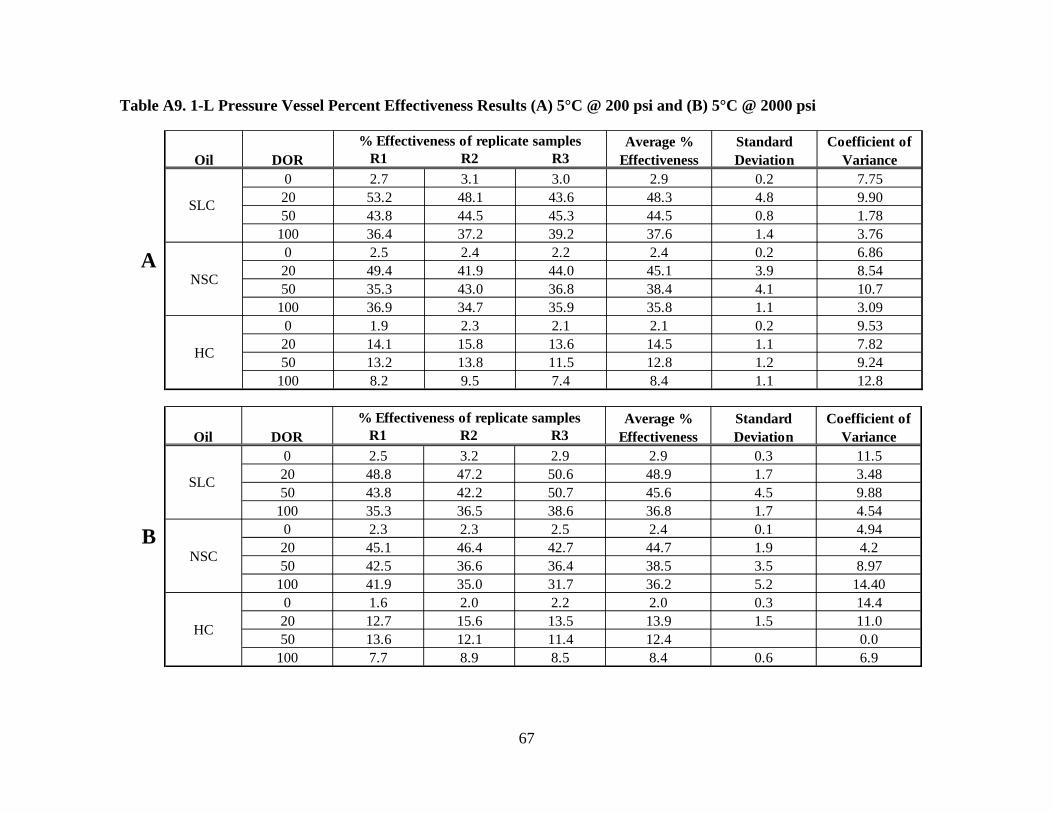
Table A9. 1-L Pressure Vessel Percent Effectiveness Results (A) 5°C @ 200 psi and (B) 5°C @ 2000 psi
Oil DOR R1 R2 R3 % Effectiveness of replicate samples Average %
Effectiveness Standard Deviation
Coefficient of Variance
SLC
0 2.7 3.1 3.0 2.9 0.2 7.75 20 53.2 48.1 43.6 48.3 4.8 9.90 50 43.8 44.5 45.3 44.5 0.8 1.78
100 36.4 37.2 39.2 37.6 1.4 3.76
NSC
0 2.5 2.4 2.2 2.4 0.2 6.86 20 49.4 41.9 44.0 45.1 3.9 8.54 50 35.3 43.0 36.8 38.4 4.1 10.7
100 36.9 34.7 35.9 35.8 1.1 3.09
HC
0 1.9 2.3 2.1 2.1 0.2 9.53 20 14.1 15.8 13.6 14.5 1.1 7.82 50 13.2 13.8 11.5 12.8 1.2 9.24
100 8.2 9.5 7.4 8.4 1.1 12.8
A
Oil DOR R1 R2 R3 % Effectiveness of replicate samples Average %
Effectiveness Standard Deviation
Coefficient of Variance
SLC
0 2.5 3.2 2.9 2.9 0.3 11.5 20 48.8 47.2 50.6 48.9 1.7 3.48 50 43.8 42.2 50.7 45.6 4.5 9.88
100 35.3 36.5 38.6 36.8 1.7 4.54
NSC
0 2.3 2.3 2.5 2.4 0.1 4.94 20 45.1 46.4 42.7 44.7 1.9 4.2 50 42.5 36.6 36.4 38.5 3.5 8.97
100 41.9 35.0 31.7 36.2 5.2 14.40
HC
0 1.6 2.0 2.2 2.0 0.3 14.4 20 12.7 15.6 13.5 13.9 1.5 11.0 50 13.6 12.1 11.4 12.4 0.0
100 7.7 8.9 8.5 8.4 0.6 6.9
B
67

Table A10. 1-L Pressure Vessel Percent Effectiveness Results (A) 23°C @ 200 psi and (B) 23°C @ 2000 psi
Oil DOR R1 R2 R3 % Effectiveness of replicate samples Average %
Effectiveness Standard Deviation
Coefficient of Variance
SLC
0 3.42 4.02 3.75 3.7 0.3 8.1 20 60.4 57.9 52.7 57.0 3.9 6.9 50 50.3 57.5 53.8 53.9 3.6 6.7
100 50.9 49.8 54.5 51.7 2.5 4.8
NSC
0 2.89 3.21 2.51 2.9 0.4 12.2 20 56.1 49.3 54.3 53.2 3.5 6.6 50 42.9 50.6 43.8 45.8 4.2 9.2
100 40.1 38.7 42.5 40.4 1.9 4.8
HC
0 2.39 2.84 2.55 2.6 0.2 8.8 20 15.8 17.5 14.3 15.9 1.6 10.1 50 14.7 16.2 12.4 14.4 1.9 13.3
100 10.5 11.9 9.7 10.7 1.1 10.4
A
Oil DOR R1 R2 R3 % Effectiveness of replicate samples Average %
Effectiveness Standard Deviation
Coefficient of Variance
SLC
0 3.2 3.9 3.6 3.6 0.4 10.3 20 59.4 50.9 56.4 55.6 4.3 7.7 50 53.6 57.7 48.9 53.4 4.4 8.3
100 48.6 44.3 41.8 44.9 3.4 7.6
NSC
0 2.5 2.9 3.3 2.9 0.4 12.8 20 51.2 63.5 54.5 56.4 6.4 11.3 50 44.9 48.9 42.1 45.3 3.4 7.6
100 39.3 36.2 41.1 38.8 2.5 6.3
HC
0 2.0 2.5 2.8 2.4 0.4 17.5 20 15.3 15.1 17.8 16.1 1.5 9.4 50 12.9 14.0 13.4 13.4 0.6 4.1
100 12.5 8.4 9.4 10.1 2.2 21.4
B
68
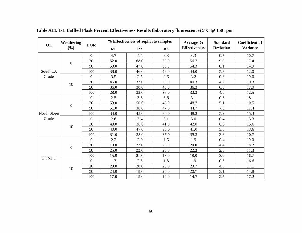
Table A11. 1-L Baffled Flask Percent Effectiveness Results (laboratory fluorescence) 5°C @ 150 rpm.
Oil Weathering
(%) DOR
R1 R2 R3
% Effectiveness of replicate samples Average % Effectiveness
Standard Deviation
Coefficient of Variance
South LA Crude
0
0 4.7 4.4 3.8 4.3 0.5 10.7 20 52.0 68.0 50.0 56.7 9.9 17.4 50 53.0 47.0 63.0 54.3 8.1 14.9 100 38.0 46.0 48.0 44.0 5.3 12.0
10
0 3.5 2.5 3.6 3.2 0.6 19.0 20 45.0 37.0 39.0 40.3 4.2 10.3 50 36.0 30.0 43.0 36.3 6.5 17.9 100 28.0 33.0 36.0 32.3 4.0 12.5
North Slope Crude
0
0 2.5 3.3 3.6 3.1 0.6 18.1 20 53.0 50.0 43.0 48.7 5.1 10.5 50 51.0 36.0 47.0 44.7 7.8 17.4 100 34.0 45.0 36.0 38.3 5.9 15.3
10
0 2.6 3.4 3.1 3.0 0.4 13.3 20 49.0 36.0 41.0 42.0 6.6 15.6 50 40.0 47.0 36.0 41.0 5.6 13.6 100 31.0 38.0 37.0 35.3 3.8 10.7
HONDO
0
0 2.2 2.0 1.5 1.9 0.4 19.0 20 19.0 27.0 26.0 24.0 4.4 18.2 50 25.0 22.0 20.0 22.3 2.5 11.3 100 15.0 21.0 18.0 18.0 3.0 16.7
10
0 1.7 2.3 1.8 1.9 0.3 16.6 20 23.0 20.0 28.0 23.7 4.0 17.1 50 24.0 18.0 20.0 20.7 3.1 14.8 100 17.0 15.0 12.0 14.7 2.5 17.2
69

Table A12. 1-L Baffled Flask Percent Effectiveness Results (laboratory fluorescence) 5°C @ 200 rpm.
Oil Weathering
(%) DOR
R1 R2 R3
% Effectiveness of replicate samples Average % Effectiveness
Standard Deviation
Coefficient of Variance
South LA Crude
0
0 6.9 5.8 6.3 6.3 0.6 8.70 20 88.0 87.0 70.0 81.7 10.1 12.39 50 71.0 85.0 77.0 77.7 7.0 9.04 100 74.0 55.0 60.0 63.0 9.8 15.63
10
0 5.8 6.2 5.0 5.7 0.6 10.78 20 82.0 66.0 74.0 74.0 8.0 10.81 50 63.0 82.0 71.0 72.0 9.5 13.25 100 66.0 71.0 56.0 64.3 7.6 11.87
North Slope Crude
0
0 5.2 4.1 3.8 4.4 0.7 16.88 20 66.0 70.0 79.0 71.7 6.7 9.29 50 63.0 62.0 73.0 66.0 6.1 9.2 100 50.0 67.0 53.0 56.7 9.1 16.01
10
0 2.9 3.7 4.1 3.6 0.6 17.13 20 77.0 62.0 69.0 69.3 7.5 10.83 50 67.0 51.0 63.0 60.3 8.3 13.80 100 52.0 49.0 61.0 54.0 6.2 11.56
HONDO
0
0 1.7 2.1 1.7 1.8 0.2 12.60 20 25.0 32.0 26.0 27.7 3.8 13.68 50 26.0 29.0 21.0 25.3 4.0 15.95 100 23.0 16.0 20.0 19.7 3.5 17.86
10
0 2.1 1.5 1.8 1.8 0.3 16.67 20 25.0 21.0 28.0 24.7 3.5 14.24 50 20.0 26.0 24.0 23.3 3.1 13.09 100 16.0 23.0 20.0 19.7 3.5 17.9
70

Table A13. 1-L Baffled Flask Percent Effectiveness Results (laboratory fluorescence) 23°C @ 150 rpm.
Oil Weathering
(%) DOR
R1 R2 R3
% Effectiveness of replicate samples Average % Effectiveness
Standard Deviation
Coefficient of Variance
South LA Crude
0
0 6.0 5.3 5.0 5.4 0.5 9.44 20 64.0 65.0 76.0 68.3 6.7 9.74 50 52.0 65.0 66.0 61.0 7.8 12.80 100 58.0 48.0 53.0 53.0 5.0 9.43
10
0 5.1 4.0 3.5 4.2 0.8 19.49 20 53.0 59.0 47.0 53.0 6.0 11.32 50 44.0 56.0 49.0 49.7 6.0 12.14 100 52.0 42.0 36.0 43.3 8.1 18.65
North Slope Crude
0
0 3.8 3.2 4.6 3.9 0.7 18.16 20 54.0 68.0 57.0 59.7 7.4 12.35 50 50.0 49.0 63.0 54.0 7.8 14.5 100 58.0 45.0 43.0 48.7 8.1 16.74
10
0 4.7 3.4 4.4 4.2 0.7 16.34 20 44.0 59.0 57.0 53.3 8.1 15.27 50 50.0 56.0 42.0 49.3 7.0 14.24 100 52.0 41.0 38.0 43.7 7.4 16.88
HONDO
0
0 2.0 1.4 1.9 1.8 0.3 18.20 20 34.0 27.0 25.0 28.7 4.7 16.49 50 26.0 24.0 31.0 27.0 3.6 13.35 100 26.0 22.0 18.0 22.0 4.0 18.18
10
0 2.3 1.9 2.0 2.1 0.2 10.07 20 31.0 24.0 29.0 28.0 3.6 12.88 50 25.0 19.0 26.0 23.3 3.8 16.23 100 20.0 22.0 16.0 19.3 3.1 15.80
71

Table A14. 1-L Baffled Flask Percent Effectiveness Results (laboratory fluorescence) 23°C @ 200 rpm.
Oil Weathering
(%) DOR
R1 R2 R3
% Effectiveness of replicate samples Average % Effectiveness
Standard Deviation
Coefficient of Variance
South LA Crude
0
0 9.2 8.2 8.1 8.5 0.6 7.16 20 97.0 83.0 95.0 91.7 7.6 8.26 50 75.0 85.0 91.0 83.7 8.1 9.66 100 77.0 86.0 73.0 78.7 6.7 8.46
10
0 7.7 6.9 6 6.9 0.9 12.39 20 91.0 78.0 76.0 81.7 8.1 9.97 50 86.0 66.0 73.0 75.0 10.1 13.53 100 65.0 69.0 80.0 71.3 7.8 10.89
North Slope Crude
0
0 6.2 4.9 5.6 5.6 0.7 11.69 20 89.0 74.0 71.0 78.0 9.6 12.36 50 65.0 77.0 74.0 72.0 6.2 8.67 100 51.0 68.0 64.0 61.0 8.9 14.57
10
0 4.8 4.2 3.7 4.2 0.6 13.01 20 73.0 82.0 67.0 74.0 7.5 10.20 50 69.0 75.0 58.0 67.3 8.6 12.80 100 53.0 67.0 62.0 60.7 7.1 11.69
HONDO
0
0 2.6 2.2 1.9 2.2 0.4 15.72 20 35.0 37.0 30.0 34.0 3.6 10.60 50 26.0 34.0 29.0 29.7 4.0 13.62 100 29.0 26.0 21.0 25.3 4.0 15.95
10
0 2.7 1.9 2.4 2.3 0.4 17.32 20 30.0 34.0 27.0 30.3 3.5 11.58 50 26.0 33.0 24.0 27.7 4.7 17.08 100 27.0 23.0 21.0 23.7 3.1 12.91
72
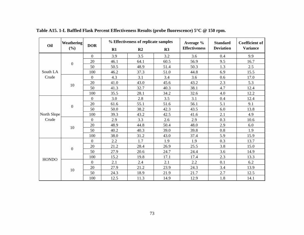
Table A15. 1-L Baffled Flask Percent Effectiveness Results (probe fluorescence) 5°C @ 150 rpm.
Oil Weathering
(%) DOR
R1 R2 R3
% Effectiveness of replicate samples Average % Effectiveness
Standard Deviation
Coefficient of Variance
South LA Crude
0
0 3.9 3.5 3.2 3.6 0.4 9.9 20 46.1 64.1 60.5 56.9 9.5 16.7 50 50.5 48.9 51.4 50.3 1.3 2.5
100 46.2 37.3 51.0 44.8 6.9 15.5
10
0 4.3 3.1 3.4 3.6 0.6 17.0 20 41.0 43.0 45.6 43.2 2.3 5.3 50 41.3 32.7 40.3 38.1 4.7 12.4
100 35.5 28.1 34.2 32.6 4.0 12.2
North Slope Crude
0
0 3.0 2.8 3.5 3.1 0.4 12.4 20 61.6 55.1 51.6 56.1 5.1 9.1 50 50.0 38.2 42.3 43.5 6.0 13.8
100 39.3 43.2 42.5 41.6 2.1 4.9
10
0 2.9 3.3 2.6 2.9 0.3 10.6 20 48.9 44.8 50.4 48.0 2.9 6.0 50 40.2 40.3 39.0 39.8 0.8 1.9
100 38.0 31.2 43.0 37.4 5.9 15.9
HONDO
0
0 2.2 1.7 1.9 1.9 0.3 13.7 20 21.2 28.4 26.9 25.5 3.8 15.0 50 27.9 20.6 24.7 24.4 3.6 14.9
100 15.2 19.8 17.1 17.4 2.3 13.3
10
0 2.1 2.4 2.1 2.2 0.1 6.2 20 27.9 21.2 23.9 24.3 3.4 13.9 50 24.3 18.9 21.9 21.7 2.7 12.5
100 12.5 11.3 14.9 12.9 1.8 14.1
73

Table A16. 1-L Baffled Flask Percent Effectiveness Results (probe fluorescence) 5°C @ 200 rpm.
Oil Weathering
(%) DOR
R1 R2 R3
% Effectiveness of replicate samples Average % Effectiveness
Standard Deviation
Coefficient of Variance
South LA Crude
0
0 7.5 5.7 7.4 6.9 1.0 14.90 20 78.4 72.7 83.0 78.1 5.2 6.60 50 79.1 77.0 81.0 79.0 2.0 2.53
100 64.2 61.4 50.8 58.8 7.1 12.06
10
0 6.7 6.6 4.9 6.1 1.0 16.35 20 77.4 68.8 90.0 78.7 10.7 13.53 50 68.4 89.0 66.2 74.5 12.6 16.85
100 62.1 76.0 68.6 68.9 6.9 10.07
North Slope Crude
0
0 3.9 4.9 4.5 4.4 0.5 11.70 20 77.6 71.7 70.7 73.3 3.7 5.09 50 63.4 69.1 61.5 64.7 3.9 6.1
100 42.3 57.9 59.2 53.1 9.4 17.70
10
0 3.6 2.9 3.8 3.4 0.5 13.39 20 76.5 59.6 60.9 65.7 9.4 14.31 50 70.5 52.4 64.7 62.5 9.3 14.80
100 58.0 48.0 51.0 52.3 5.1 9.83
HONDO
0
0 2.0 1.6 2.0 1.9 0.2 12.35 20 26.3 28.5 31.8 28.8 2.8 9.68 50 28.1 31.2 26.3 28.5 2.5 8.66
100 22.3 18.4 25.7 22.1 3.7 16.50
10
0 1.9 1.6 1.7 1.7 0.2 9.15 20 27.4 20.1 22.4 23.3 3.7 15.93 50 22.1 26.6 27.8 25.5 3.0 11.85
100 17.0 19.6 17.6 18.1 1.4 7.6
74
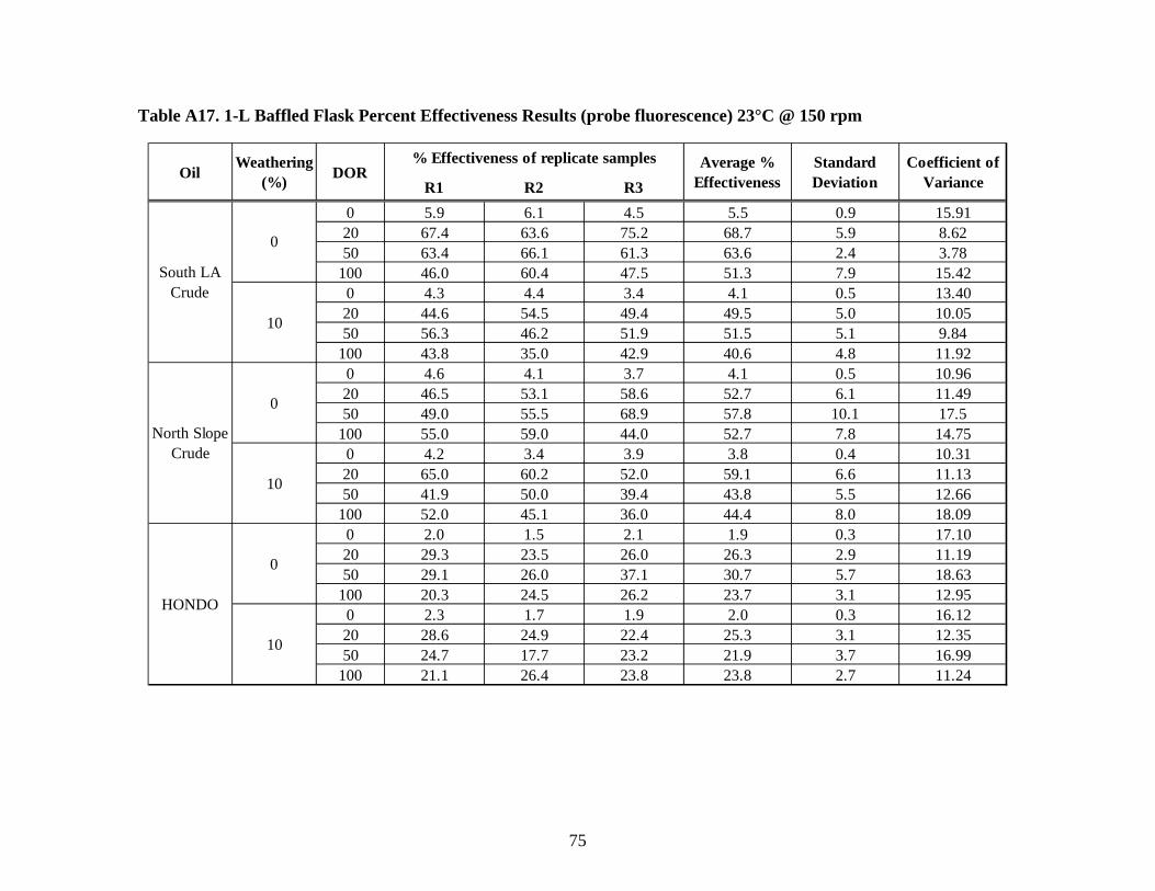
Table A17. 1-L Baffled Flask Percent Effectiveness Results (probe fluorescence) 23°C @ 150 rpm
Oil Weathering
(%) DOR
R1 R2 R3
% Effectiveness of replicate samples Average % Effectiveness
Standard Deviation
Coefficient of Variance
South LA Crude
0
0 5.9 6.1 4.5 5.5 0.9 15.91 20 67.4 63.6 75.2 68.7 5.9 8.62 50 63.4 66.1 61.3 63.6 2.4 3.78
100 46.0 60.4 47.5 51.3 7.9 15.42
10
0 4.3 4.4 3.4 4.1 0.5 13.40 20 44.6 54.5 49.4 49.5 5.0 10.05 50 56.3 46.2 51.9 51.5 5.1 9.84
100 43.8 35.0 42.9 40.6 4.8 11.92
North Slope Crude
0
0 4.6 4.1 3.7 4.1 0.5 10.96 20 46.5 53.1 58.6 52.7 6.1 11.49 50 49.0 55.5 68.9 57.8 10.1 17.5
100 55.0 59.0 44.0 52.7 7.8 14.75
10
0 4.2 3.4 3.9 3.8 0.4 10.31 20 65.0 60.2 52.0 59.1 6.6 11.13 50 41.9 50.0 39.4 43.8 5.5 12.66
100 52.0 45.1 36.0 44.4 8.0 18.09
HONDO
0
0 2.0 1.5 2.1 1.9 0.3 17.10 20 29.3 23.5 26.0 26.3 2.9 11.19 50 29.1 26.0 37.1 30.7 5.7 18.63
100 20.3 24.5 26.2 23.7 3.1 12.95
10
0 2.3 1.7 1.9 2.0 0.3 16.12 20 28.6 24.9 22.4 25.3 3.1 12.35 50 24.7 17.7 23.2 21.9 3.7 16.99
100 21.1 26.4 23.8 23.8 2.7 11.24
75

Table A18. 1-L Baffled Flask Percent Effectiveness Results (probe fluorescence) 23°C @ 200 rpm.
Oil Weathering
(%) DOR
R1 R2 R3
% Effectiveness of replicate samples Average % Effectiveness
Standard Deviation
Coefficient of Variance
South LA Crude
0
0 8.4 7.6 8.6 8.2 0.5 6.45 20 90.3 84.0 87.9 87.4 3.2 3.67 50 79.1 86.0 77.7 80.9 4.5 5.51
100 90.8 70.6 67.7 76.4 12.6 16.48
10
0 6.6 7.2 5.1 6.3 1.1 17.02 20 88.5 78.2 65.7 77.5 11.4 14.74 50 69.6 87.7 63.3 73.5 12.6 17.20
100 71.4 69.4 75.0 71.9 2.8 3.95
North Slope Crude
0
0 5.2 5.9 4.8 5.3 0.6 10.38 20 83.4 62.5 87.5 77.8 13.4 17.29 50 74.5 61.4 75.0 70.3 7.7 10.94
100 62.0 63.9 75.9 67.3 7.5 11.23
10
0 4.8 4.7 3.8 4.5 0.5 11.85 20 64.8 75.6 78.2 72.9 7.1 9.75 50 69.8 73.9 59.2 67.6 7.6 11.21
100 61.4 61.9 57.5 60.3 2.4 4.00
HONDO
0
0 2.6 1.9 2.3 2.2 0.4 16.34 20 38.5 40.3 31.3 36.7 4.8 13.03 50 24.7 33.3 27.1 28.4 4.4 15.59
100 30.3 27.6 23.8 27.2 3.2 11.93
10
0 2.4 2.1 2.9 2.5 0.4 16.55 20 36.3 26.4 31.6 31.4 5.0 15.89 50 22.2 28.4 29.3 26.6 3.9 14.60
100 26.1 21.8 25.3 24.4 2.3 9.35
76

Table A19. 1-L Baffled Flask Percent Effectiveness Results (turbidity) 5°C @ 150 rpm.
Oil Weathering
(%) DOR
R1 R2 R3
% Effectiveness of replicate samples Average % Effectiveness
Standard Deviation
Coefficient of Variance
South LA Crude
0
0 5.2 3.9 3.1 4.0 1.1 26.3 20 64.4 67.9 51.5 61.3 8.6 14.1 50 70.6 55.3 82.4 69.4 13.6 19.6
100 38.0 67.5 66.5 57.3 16.8 29.3
10
0 3.2 2.6 3.0 3.0 0.3 11.4 20 61.5 44.2 51.1 52.3 8.7 16.6 50 45.1 42.7 58.8 48.8 8.7 17.8
100 38.3 41.7 49.9 43.3 6.0 13.8
North Slope Crude
0
0 2.4 2.9 3.7 3.0 0.6 20.5 20 64.0 48.1 33.3 48.5 15.4 31.7 50 66.0 36.7 42.4 48.4 15.5 32.1
100 24.5 56.2 38.1 39.6 15.9 40.0
10
0 2.8 3.4 2.3 2.9 0.5 18.8 20 64.0 43.1 36.9 48.0 14.2 29.6 50 38.0 26.0 35.9 33.3 6.4 19.2
100 42.0 29.8 47.0 39.6 8.9 22.4
HONDO
0
0 1.7 2.2 1.7 1.9 0.3 16.4 20 12.8 27.3 25.9 22.0 8.0 36.4 50 15.0 13.7 9.5 12.7 2.9 22.7
100 20.9 17.2 18.0 18.7 1.9 10.3
10
0 1.4 2.0 2.1 1.8 0.4 21.0 20 22.9 28.7 20.7 24.1 4.2 17.3 50 14.7 8.8 14.7 12.7 3.4 26.8
100 5.8 10.6 9.3 8.6 2.5 29.0
77
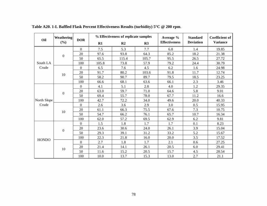
Table A20. 1-L Baffled Flask Percent Effectiveness Results (turbidity) 5°C @ 200 rpm.
Oil Weathering
(%) DOR
R1 R2 R3
% Effectiveness of replicate samples Average % Effectiveness
Standard Deviation
Coefficient of Variance
South LA Crude
0
0 7.5 5.3 7.7 6.8 1.4 19.85 20 97.6 93.8 64.3 85.2 18.2 21.38 50 65.5 115.4 105.7 95.5 26.5 27.72
100 105.8 73.8 57.9 79.2 24.4 30.79
10
0 6.5 7.6 4.5 6.2 1.6 24.98 20 91.7 80.2 103.6 91.8 11.7 12.74 50 58.2 90.7 89.7 79.5 18.5 23.25
100 66.6 68.1 63.6 66.1 2.3 3.46
North Slope Crude
0
0 4.1 5.1 2.8 4.0 1.2 29.35 20 63.0 59.7 71.0 64.6 5.8 9.01 50 69.4 55.7 78.0 67.7 11.2 16.6
100 42.7 72.2 34.0 49.6 20.0 40.33
10
0 2.6 3.6 2.9 3.0 0.5 15.95 20 61.1 66.3 75.5 67.6 7.3 10.75 50 54.7 66.2 76.1 65.7 10.7 16.34
100 62.0 57.2 69.5 62.9 6.2 9.81
HONDO
0
0 1.5 1.8 1.7 1.7 0.1 8.23 20 23.6 30.6 24.0 26.1 3.9 15.04 50 29.3 39.1 31.2 33.2 5.2 15.67
100 22.3 21.8 16.0 20.0 3.5 17.52
10
0 2.7 1.8 1.7 2.1 0.6 27.25 20 21.4 14.1 26.1 20.5 6.0 29.41 50 11.6 15.2 20.5 15.7 4.5 28.54
100 10.0 13.7 15.3 13.0 2.7 21.1
78

Table A21. 1-L Baffled Flask Percent Effectiveness Results (turbidity) 23°C @ 150 rpm.
Oil Weathering
(%) DOR
R1 R2 R3
% Effectiveness of replicate samples Average % Effectiveness
Standard Deviation
Coefficient of Variance
South LA Crude
0
0 3.9 5.4 3.2 4.2 1.1 27.57 20 54.8 76.1 54.0 61.6 12.5 20.35 50 53.4 51.0 88.8 64.4 21.2 32.87
100 37.4 54.3 64.3 52.0 13.6 26.14
10
0 3.4 2.0 3.7 3.0 0.9 30.84 20 53.4 57.0 41.5 50.6 8.1 15.99 50 42.6 55.2 63.2 53.6 10.4 19.38
100 37.6 38.3 42.5 39.5 2.6 6.69
North Slope Crude
0
0 4.8 3.9 3.8 4.2 0.5 12.53 20 52.5 81.1 68.6 67.4 14.3 21.21 50 48.7 46.9 67.7 54.4 11.5 21.1
100 59.2 53.8 52.3 55.1 3.6 6.62
10
0 3.4 2.6 4.1 3.4 0.8 22.39 20 41.8 69.8 46.7 52.7 15.0 28.38 50 49.6 63.4 46.7 53.2 8.9 16.80
100 51.9 52.8 42.1 48.9 5.9 12.08
HONDO
0
0 2.0 1.3 1.8 1.7 0.4 21.06 20 29.1 24.0 31.8 28.3 4.0 14.05 50 15.4 24.0 20.8 20.1 4.4 21.81
100 24.8 28.3 17.9 23.7 5.3 22.41
10
0 2.5 1.6 1.3 1.8 0.6 35.65 20 18.0 24.1 28.7 23.6 5.3 22.66 50 30.5 24.2 25.9 26.9 3.3 12.12
100 14.3 25.8 22.6 20.9 5.9 28.46
79

Table A22. 1-L Baffled Flask Percent Effectiveness Results (turbidity) 23°C @ 200 rpm.
Oil Weathering
(%) DOR
R1 R2 R3
% Effectiveness of replicate samples Average % Effectiveness
Standard Deviation
Coefficient of Variance
South LA Crude
0
0 7.7 4.7 7.3 6.6 1.6 24.80 20 105.9 92.5 79.0 92.5 13.5 14.57 50 89.1 81.4 93.9 88.2 6.3 7.12
100 71.5 63.1 55.9 63.5 7.8 12.27
10
0 6.3 7.1 5.635 6.3 0.8 11.87 20 97.5 86.4 95.0 93.0 5.8 6.27 50 57.9 116.1 91.4 88.5 29.2 32.97
100 70.5 72.1 64.1 68.9 4.3 6.18
North Slope Crude
0
0 6.2 3.9 6.2 5.4 1.3 24.02 20 71.5 58.2 55.3 61.6 8.6 13.99 50 51.9 71.4 66.1 63.1 10.1 15.92
100 38.0 76.2 79.9 64.7 23.2 35.85
10
0 4.8 4.5 4.4 4.6 0.2 4.88 20 92.9 91.2 69.5 84.6 13.0 15.41 50 61.1 85.5 50.1 65.5 18.1 27.68
100 56.8 76.4 63.4 65.6 10.0 15.23
HONDO
0
0 3.1 1.9 1.5 2.2 0.9 39.31 20 35.4 34.5 23.1 31.0 6.8 22.00 50 33.2 21.5 29.1 27.9 5.9 21.18
100 25.1 18.0 27.7 23.6 5.0 21.29
10
0 1.7 1.7 2.5 2.0 0.4 22.76 20 37.5 33.0 18.9 29.8 9.7 32.59 50 20.0 18.4 25.1 21.2 3.5 16.52
100 23.5 23.1 30.0 25.5 3.8 15.01
80

Con
cent
ratio
n (p
pm)
0
5
10
15
20
25
30
Y = 0.005X - 0.4606 R2 = 0.9985
A
0 1000 2000 3000 4000 5000 6000
Response
Con
cent
ratio
n (p
pm)
0
5
10
15
20
25
30
Y = 0.0041X - 0.7007 R2 = 0.9967
B
0 1000 2000 3000 4000 5000 6000 7000
Response
Con
cent
ratio
n (p
pm)
0
2
4
6
8
10
12
14
Y = 0.0044X - 0.5145 R2 = 0.9942
C
0 500 1000 1500 2000 2500 3000 3500
Response
Figure A1. Laboratory Fluorescence Curves: (A) South Louisiana crude, (B) North Slope crude, and (C) Hondo crude.
81

Con
cent
ratio
n (p
pm)
0
200
400
600
800
1000
1200
Y = 17.363X - 8.1428 R2 = 0.999
A
0 10 20 30 40 50 60 70
Response
Con
cent
ratio
n (p
pm)
0
200
400
600
800
1000
1200
Y = 8.9522X - 5.3042 R2 = 0.999
B
0 20 40 60 80 100 120
Response
Con
cent
ratio
n (p
pm)
0
200
400
600
800
1000
1200
Y = 5.2978X - 5.1505 R2 = 0.999
C
0 20 40 60 80 100 120 140 160 180 200
Response
Figure A2. Laboratory UV-Vis Curves: (A) South Louisiana crude, (B) North Slope crude, and (C) Hondo crude.
82

% E
ffect
iven
ess
15
10
5
0
A
Y = 0.0118X R2 = 0.9759
0 200 400 600 800 1000 1200 1400
Response (mV)
% E
ffect
iven
ess
0
2
4
6
8
10
12
14
16
Y = 0.0364X R2 = 0.9738
B
0 100 200 300 400
Response (mV)
% E
ffect
iven
ess
0
5
10
15
20
25
30
Y = 0.2017X R2 = 0.9825
C
0 20 40 60 80 100 120 140
Response (mV)
Figure A3. Field Probe Calibration Curves: (A) South Louisiana crude, (B) North Slope crude, and (C) Hondo crude. Baseline: DOR=1:20, 23°C, and 150 rpm.
83

% E
ffectiven
ess
25
20
15
10
5
0
A
Y = 0.2096X R2 = 0.9855
0 20 40 60 80 100
Response (NTU)
0 10 20 30 40 50 60 70
Response (NTU)
% E
ffect
iven
ess
0
2
4
6
8
10
12
14
16
18 B
Y = 0.2614X R2 = 0.9913
% E
ffectiven
ess
0
5
10
15
20
25
30
35 C
Y = 0.809X R2 = 0.9977
0 5 10 15 20 25 30 35 40
Response (NTU)
Figure A4. Turbidimeter Calibration Curves: (A) South Louisiana crude, (B) North Slope crude, and (C) Hondo crude. Baseline: DOR=1:20, 23°C, and 150 rpm.
84