Assessment of Rodent Glioma Models Using Magnetic Resonance Imaging Techniques

Development of Magnetic Models to
Assess Transformersrsquo Susceptibility to
Geomagnetic Disturbances
A thesis submitted to The University of Manchester for the degree of
Doctor of Philosophy
in the Faculty of Science and Engineering
2018
Yufan Ni
School of Electrical and Electronic Engineering
Contents
2
Contents
List of Figures 6
List of Tables 12
List of Abbreviations 13
List of Symbols 14
Abstracthelliphellip 17
Declarationhellip 18
Copyright Statement 19
Acknowledgement 20
Chapter 1 Introduction 21
11 Background 21
Transformer 21 111
UK power system network 22 112
Geomagnetically Induced Current 25 113
Motivations 27 114
12 Objective of research 29
13 Outline of the thesis 31
Chapter 2 Overview of Transformer Core and Winding 34
21 Overview 34
22 Transformer core 34
Core configuration 34 221
Core steel 36 222
Core losses 38 223
23 Transformer winding 41
Winding type 41 231
Winding connection 41 232
Winding material 41 233
Winding losses 42 234
24 Transformer equivalent circuit 42
Contents
3
Chapter 3 Review Literatures in Research Area of Geomagnetically Induced Current 44
31 GIC information 44
Solar activity cycle and strength 44 311
Induced electric field on earth 47 312
GIC on earth 48 313
32 Factors impact on GIC magnitude 49
33 GICrsquos impacts to power system network 52
34 GIC historical events 54
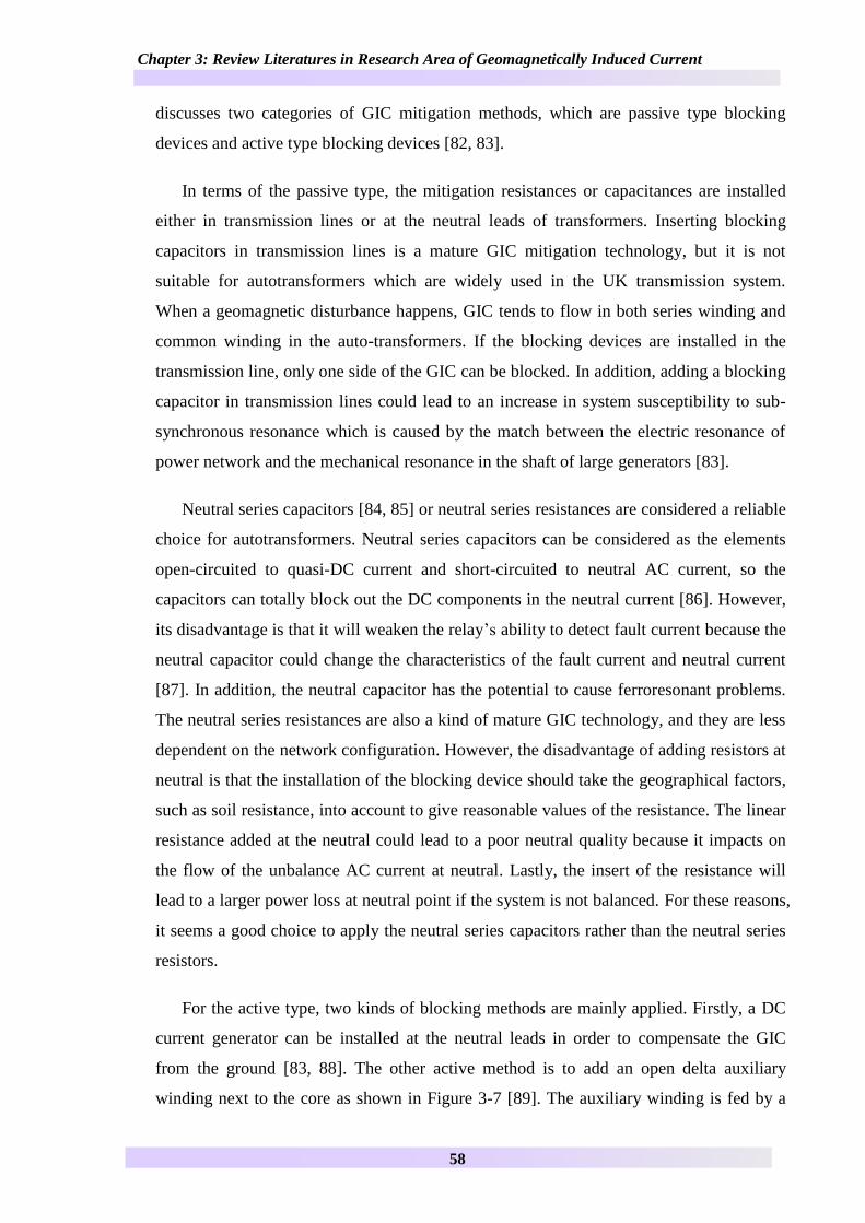
35 Mitigation of GIC 57
36 GIC experimental research 60
37 GIC simulation research 67
Individual transformer simulation by transformer models 68 371
GIC flow simulation 77 372
38 Summary 81
Chapter 4 Development of Transformer Models for GIC Simulation Studies 83
41 Introduction 83
42 Individual ATP transformer models 83
ATP simulation circuit 83 421
Transformer parameter setting 84 422
Verification of models 88 423
Summary 92 424
43 Development of new transformer model methodology and verification 93
Overview of 5-limb model 93 431
Transformer parameter setting 103 432
Simulation results under nominal AC+ 200 A DC input 105 433
Summary 119 434
Chapter 5 Sensitivity Study for New Model Parameters 120
51 Introduction 120
52 Core topology 121
Cross-sectional area ratio 121 521
53 Leakage paths 125
Contents
4
Simulation for effects of tank 125 531
Equivalent tank path length 128 532
Equivalent tank path area 129 533
Equivalent oil gap length 133 534
Equivalent oil gap area 137 535
54 Sensitivity study for winding impedance 141
HV winding resistance 141 541
TV winding resistance 145 542
HV winding leakage inductance 147 543
TV winding leakage inductance 150 544
55 Summary 153
Chapter 6 Comparison of 3-limb and 5-limb Transformer under Neutral DC Offset 155
61 Introduction 155
62 Overview of 3-limb model 155
Equivalent magnetic circuit 155 621
Transformer parameter setting 157 622
63 Simulation under AC+DC input 159
Current waveforms over whole duration 159 631
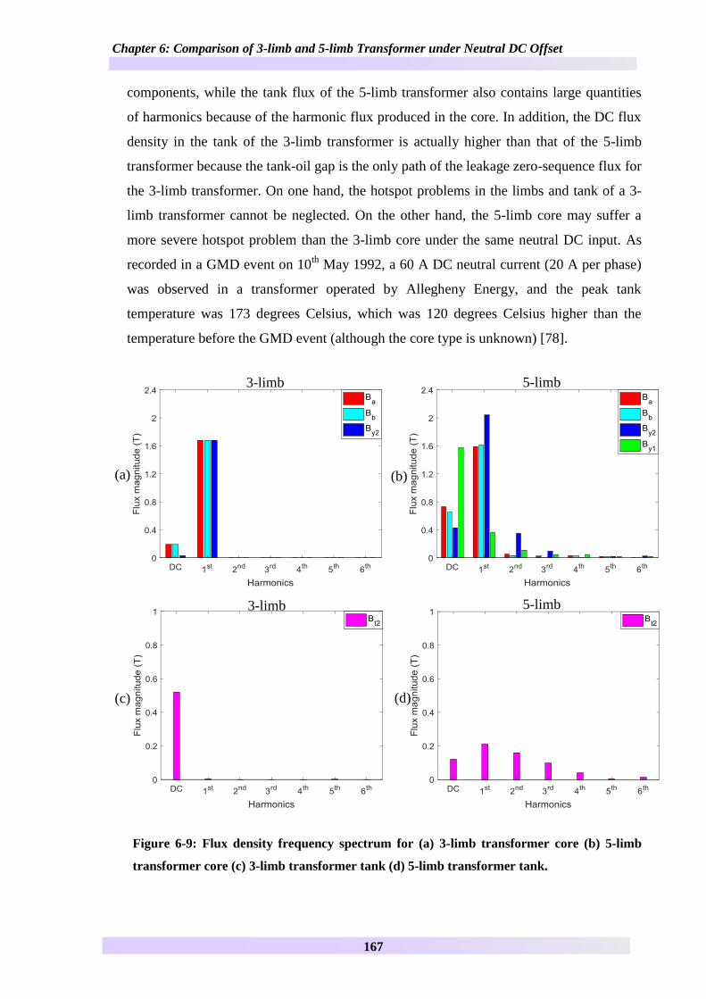
Steady state results 162 632
64 Comparison of 3-limb and 5-limb transformers under various DC inputs 168
65 Simulation in ATP 171
Under 200 A DC injection 172 651
Under different levels of DC injection 172 652
66 Summary 173
Chapter 7 Five-limb Transformer Modelling under Realistic GIC Waveforms 175
71 Introduction 175
72 Simulation for effects of delta winding 175
73 GIC simulation for 5-limb transformer 178
Case study simulation under a time varying electric field 179 731
Time varying input waveforms 183 732
GIC magnitude 186 733
Contents
5
74 Simulation with full load 188
75 Summary 191
Chapter 8 Conclusion and Future Work 193
81 Research contribution 193
82 Key findings 194
83 Future work 197
Referencehellip 199
Appendix Ihellip 205
Appendix IIhellip 206
Appendix IIIhellip 208
Appendix IVhellip 210
Appendix Vhellip 212
Appendix VI 216
Appendix VII 222
List of Figures
6
List of Figures
Figure 1-1 Schematic diagram of typical UK network [3] 23
Figure 1-2 Magnetising current for 40027513 kV 1000 MVA transformers manufactured
before the 1990s and after the 1990s in National Grid system 24
Figure 1-3 Effects of geomagnetic disturbances on Earthrsquos surface magnetic field [10] 26
Figure 2-1 Three-phase transformer core forms (a) 3-limb (b) 5-limb 35
Figure 2-2 Single-phase transformer core forms (a) 2-limb (b) 3-limb (c) cruciform 36
Figure 2-3 Typical B-H curve and knee point of core material M140-27S [36] 37
Figure 2-4 Hysteresis loop [38] 38
Figure 2-5 Schematic diagram of eddy current without lamination and with lamination 39
Figure 2-6 Transformer core lamination with 14 steps [3] 40
Figure 2-7 Equivalent circuit for two winding transformer 42
Figure 3-1 GIC generation process from Space to the surface of the Earth [46] 44
Figure 3-2 Number of power system events and Kp index on March 13 1989 [52] 47
Figure 3-3 GIC flow in power system network [15] 48
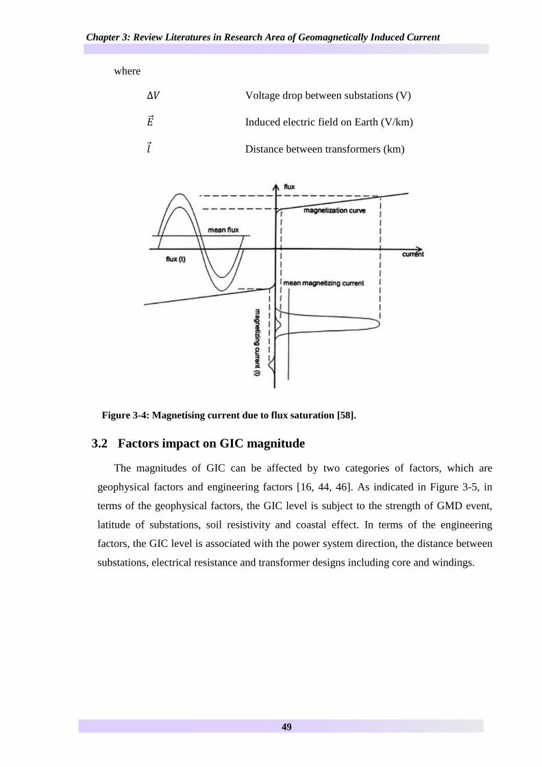
Figure 3-4 Magnetising current due to flux saturation [58] 49
Figure 3-5 Factors affecting GIC level 50
Figure 3-6 GIC historical events around the world 54
Figure 3-7 Single-phase transformer schematic with auxiliary winding [89] 59
Figure 3-8 Experimental setup for Japanese neutral DC offset test [19] 61
Figure 3-9 Input AC voltage and phase current in single-phase three-limb core [19] 61
Figure 3-10 Peak phase current against DC input in different types of transformers [19] 62
Figure 3-11 Experimental setup for Canadian neutral DC offset test [91] 63
Figure 3-12 Autotransformers peak AC current against neutral DC current [91] 63
Figure 3-13 Experimental setup for Finnish neutral DC offset test [13] 65
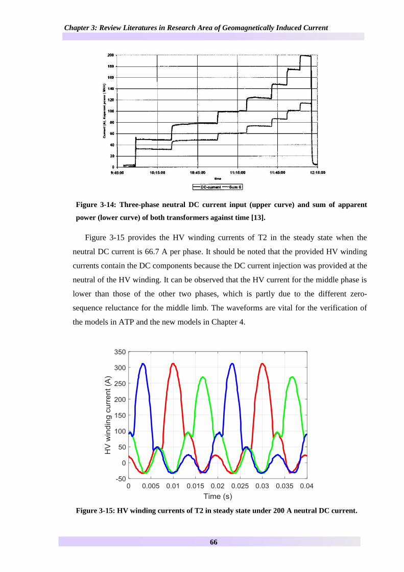
Figure 3-14 Three-phase neutral DC current input (upper curve) and sum of apparent power
(lower curve) of both transformers against time [13] 66
Figure 3-15 HV winding currents of T2 in steady state under 200 A neutral DC current 66
Figure 3-16 Temperature rise at flitch plate under the step-up DC injection 67
Figure 3-17 (a) Single-phase two legged transformer model (b) Equivalent circuit of
magnetic core model [93] 69
Figure 3-18 Three-limb YNd connected transformer model with zero sequence path and
leakage flux path [26] 70
Figure 3-19 Three-phase primary current under AC+DC input [26] 71
Figure 3-20 Single-phase transformer banks with only DC current injection with 75
residual flux [26] 72
Figure 3-21 Schematic diagram for BCTRAN transformer model added with delta connected
core representation [95] 73
Figure 3-22 Single-phase equivalent circuit for Saturable Transformer Component [95] 74
Figure 3-23 Schematic diagram for Hybrid model [100] 75
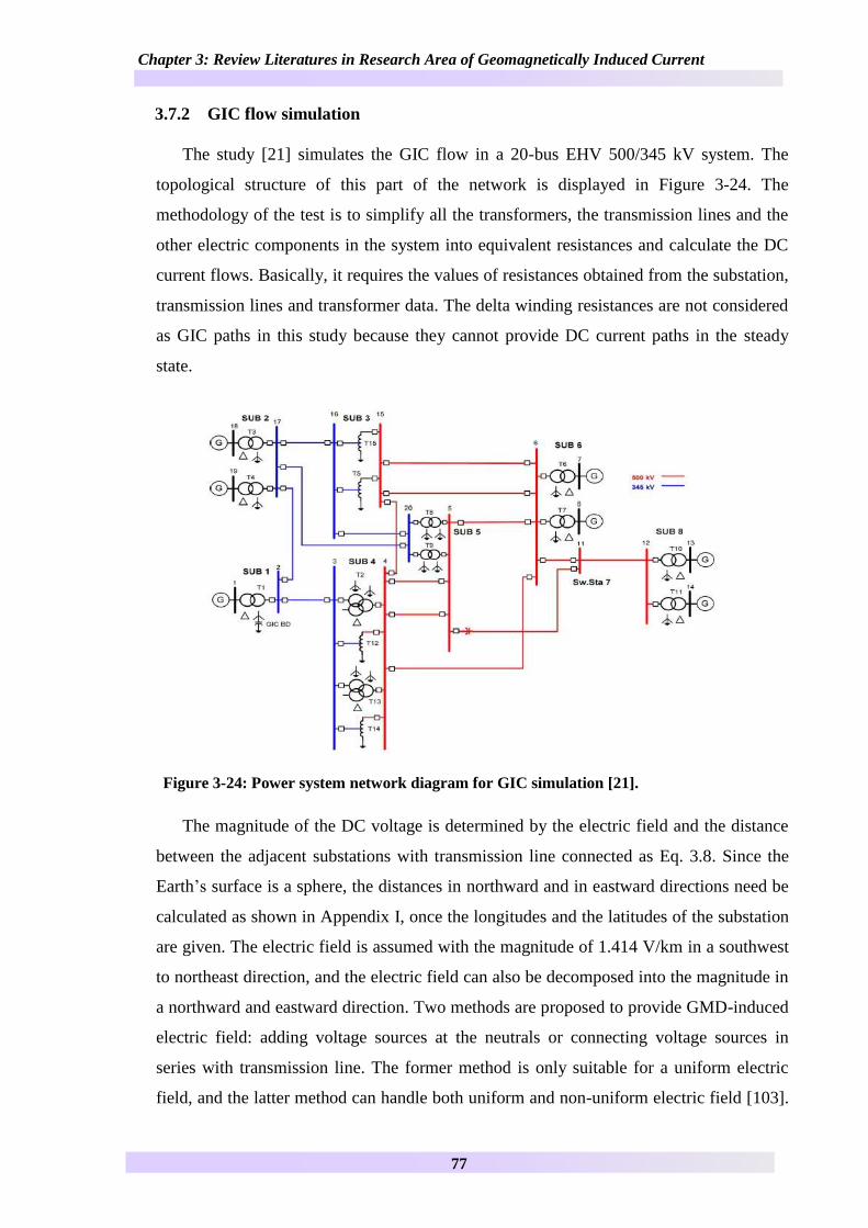
Figure 3-24 Power system network diagram for GIC simulation [21] 77
List of Figures
7
Figure 3-25 (a) GIC flows in the power system with east- west electric field (b) GIC flows
in the power system with north- south electric field [23] 80
Figure 4-1 Circuit diagram for individual transformer AC+DC simulation 84
Figure 4-2 Power system analysis tool lsquoHarmonicsrsquo 84
Figure 4-3 B-H curve of M140-27S Steel [36] 87
Figure 4-4 Core dimension of 400 kV 1000 MVA transformer 88
Figure 4-5 Comparison of HV currents between measurements and ATP models simulation
results 89
Figure 4-6 Comparisons of harmonics between measurements and ATP models simulation
results (a) Phase A magnitude (b) Phase A phase angle (c) Phase B magnitude (d) Phase B
phase angle 92
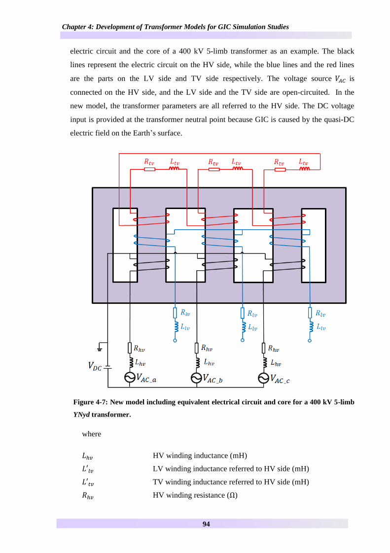
Figure 4-7 New model including equivalent electrical circuit and core for a 400 kV 5-limb
YNyd transformer 94
Figure 4-8 Schematic diagram of 5-limb transformer core including oil gaps and tank flux
paths 97
Figure 4-9 Schematic diagram of 5-limb transformer core including oil gaps and tank flux
paths 99
Figure 4-10 B-H curves of core material tank material and insulation oil 100
Figure 4-11 Flow chart of equivalent magnetic circuit calculation by using bisection method
102
Figure 4-12 Structural dimension of 5-limb core and tank 104
Figure 4-13 Phase A HV current Ihv_a (b) Phase A magnetising current Ima (c) Delta (TV)
winding current Itv_a over 30 s 106
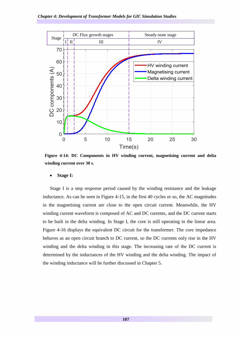
Figure 4-14 DC Components in HV winding current magnetising current and delta winding
current over 30 s 107
Figure 4-15 HV winding current magnetising current and delta winding current in Stage I
108
Figure 4-16 Simplified single-phase DC equivalent circuit in Stage I and Stage II 108
Figure 4-17 HV winding current magnetising current and delta winding current in Stage II
109
Figure 4-18 HV winding current magnetising current and delta winding current in Stage III
110
Figure 4-19 Simplified single-phase DC equivalent circuit in Stage III 110
Figure 4-20 HV winding current magnetising current and delta winding current in Stage IV
111
Figure 4-21 Simplified single-phase DC equivalent circuit in Stage IV 111
Figure 4-22 Comparison of HV currents between measurements and new model simulation
results without optimisation 112
Figure 4-23 Comparison of HV currents between measurements and new model simulation
results 113
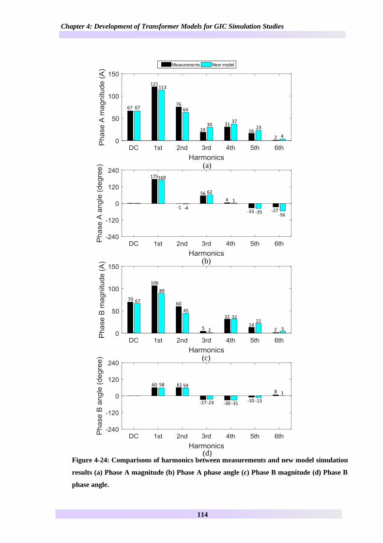
Figure 4-24 Comparisons of harmonics between measurements and new model simulation
results (a) Phase A magnitude (b) Phase A phase angle (c) Phase B magnitude (d) Phase B
phase angle 114
List of Figures
8
Figure 4-25 Comparison of Delta winding currents between measurements and new model
simulation results 115
Figure 4-26 Steady state currents and flux densities (a) Phase A HV current IA magnetising
current Ima (b) Phase B HV current IB magnetising current Imb (c) Delta (TV) winding current
Ia Ib Ic (d) flux densities of limbs and tank (e) flux densities of yokes and tank 118
Figure 4-27 Comparison of Phase B electromotive force with and without DC offset 118
Figure 5-1 (a) Phase B HV winding current (b) Delta winding current in steady state when
simulating with different yoke cross-sectional area ratio 122
Figure 5-2 (a) Phase B limb flux density and left main yoke flux density (b) Left side yoke
flux density and Phase B tank flux density in steady state when simulating with different
yoke cross-sectional area ratio 123
Figure 5-3 (a) DC components in Phase B HV winding current (b) 2nd
harmonic in Phase B
HV winding current (c) DC flux density in Phase B limb when simulating with different yoke
cross-sectional area ratio 124
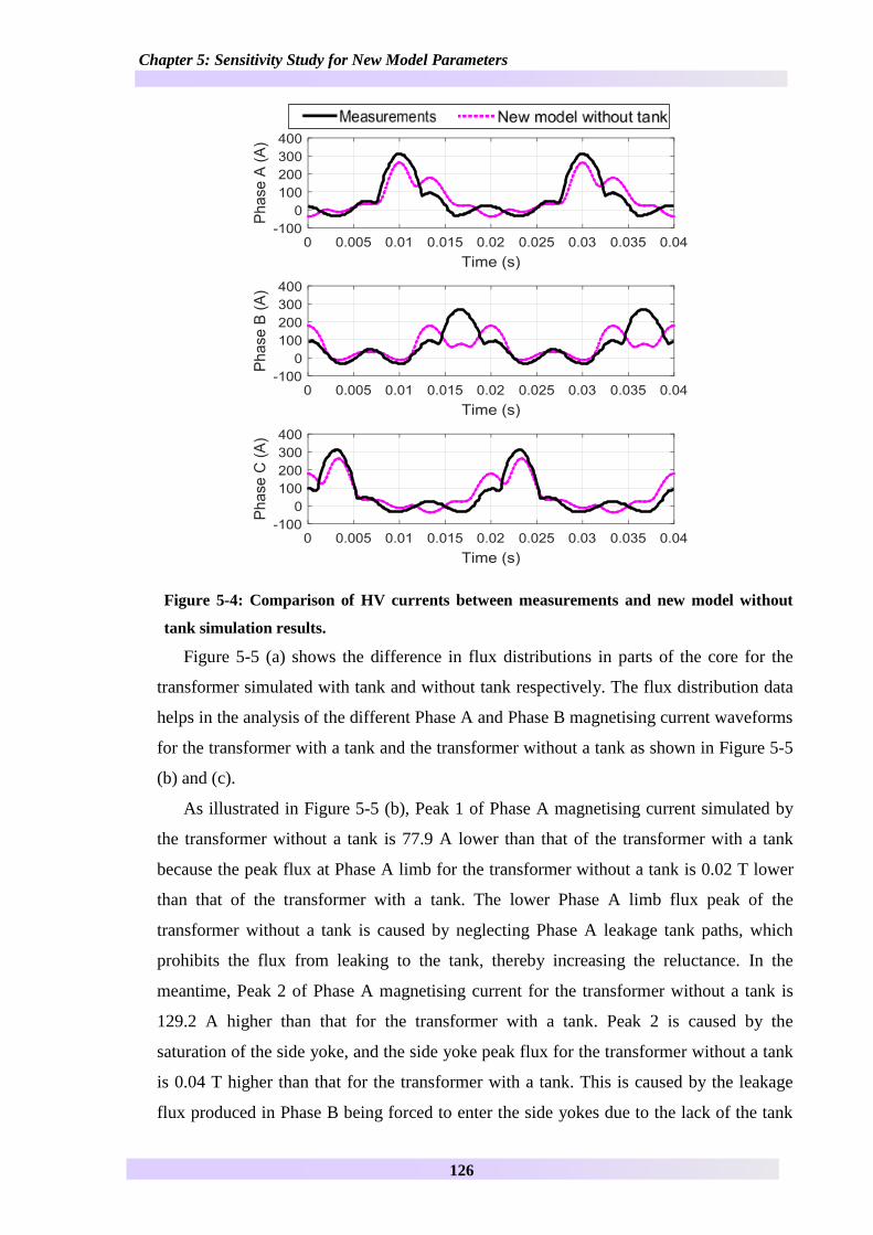
Figure 5-4 Comparison of HV currents between measurements and new model without tank
simulation results 126
Figure 5-5 Comparisons of simulation results with and without tank (a) flux distribution (b)
Phase A magnetising current (c) Phase B magnetising current 127
Figure 5-6 (a) Phase B HV winding current (b) Phase B limb flux density in steady state
when simulating with different tank path length 129
Figure 5-7 (a) Phase B HV winding current (b) Delta winding current in steady state when
simulating with different tank path area 130
Figure 5-8 (a) Phase B limb flux density and left main yoke flux density (b) Left side yoke
flux density and Phase B tank flux density in steady state when simulating with different tank
path area 131
Figure 5-9 (a) DC components in Phase B HV winding current (b) 2nd
harmonic in Phase B
HV winding current (c) DC flux density in Phase B limb when simulating with different tank
path area 132
Figure 5-10 (a) Phase B HV winding current (b) Delta winding current in steady state when
simulating with different oil gap length 134
Figure 5-11 (a) Phase B limb flux density and left main yoke flux density (b) Left side yoke
flux density and Phase B tank flux density in steady state when simulating with different oil
gap length 135
Figure 5-12 (a) DC components in Phase B HV winding current (b) 2nd
harmonic in Phase B
HV winding current (c) DC flux density in Phase B limb when simulating with different oil
gap length 136
Figure 5-13 (a) Phase B HV winding current (b) Delta winding current in steady state when
simulating with different oil gap area 138
Figure 5-14 (a) Phase B limb flux density and left main yoke flux density (b) Left side yoke
flux density and Phase B tank flux density in steady state when simulating with different oil
gap area 139
Figure 5-15 (a) DC components in Phase B HV winding current (b) 2nd
harmonic in Phase B
HV winding current (c) DC flux density in Phase B limb when simulating with different oil
gap area 140
List of Figures
9
Figure 5-16 (a) Phase B HV winding current (b) Delta winding current in steady state when
simulating with different HV winding resistance 142
Figure 5-17 (a) Phase B limb flux density and left main yoke flux density (b) Left side yoke
flux density and Phase B tank flux density in steady state when simulating with different HV
winding resistance 143
Figure 5-18 (a) DC components in Phase B HV winding current (b) 2nd
harmonic in Phase B
HV winding current (c) DC flux density in Phase B limb when simulating with different HV
winding resistance 144
Figure 5-19 (a) Phase B HV winding current (b) Delta winding current in steady state when
simulating with different TV winding resistance 145
Figure 5-20 (a) DC components in Phase B HV winding current (b) 2nd
harmonic in Phase B
HV winding current (c) DC flux density in Phase B limb when simulating with different TV
winding resistance 146
Figure 5-21 (a) Phase B HV winding current (b) delta winding current (c) Phase B limb flux
density and left main limb flux density in steady state when simulating with different HV
winding inductance 148
Figure 5-22 (a) DC components in Phase B HV winding current (b) 2nd
harmonic in Phase B
HV winding current (c) DC flux density in Phase B limb when simulating with different HV
winding inductance 149
Figure 5-23 (a) Phase B HV winding current (b) delta winding current (c) Phase B limb flux
density and left main limb flux density in steady state when simulating with different TV
winding inductance 151
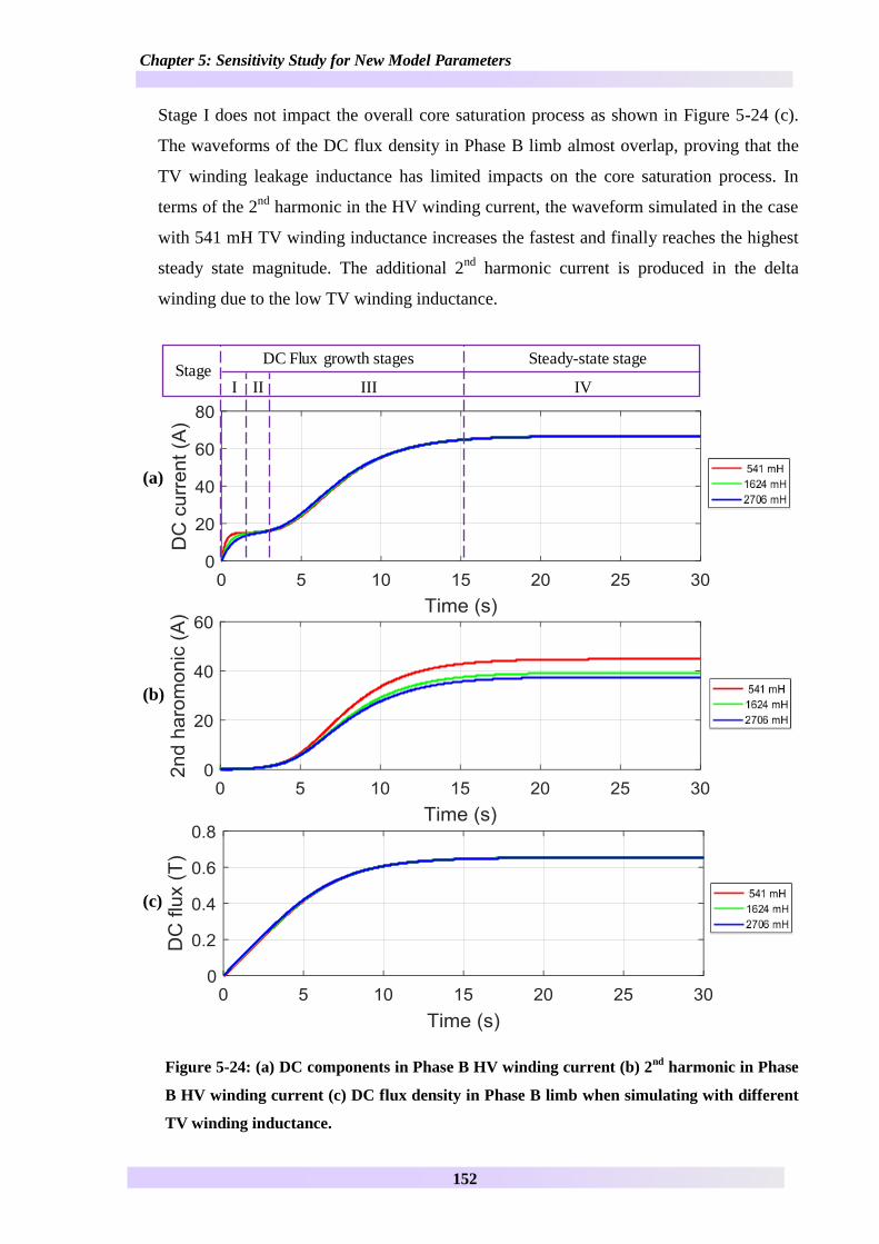
Figure 5-24 (a) DC components in Phase B HV winding current (b) 2nd
harmonic in Phase B
HV winding current (c) DC flux density in Phase B limb when simulating with different TV
winding inductance 152
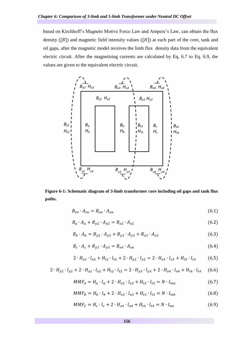
Figure 6-1 Schematic diagram of 3-limb transformer core including oil gaps and tank flux
paths 156
Figure 6-2 Schematic diagram of 3-limb transformer core including oil gaps and tank flux
paths 158
Figure 6-3 Phase A (a) HV current Ihv_a for 3-limb transformer (b) HV current Ihv_a for 5-
limb transformer (c) magnetising current Ima for 3-limb transformer (d) magnetising current
Ima for 5-limb transformer (e) Delta (TV) winding current Itv_a of 3-limb transformer (f) Delta
(TV) winding current Itv_a of 5-limb transformer over 30 s 160
Figure 6-4 DC Components in Phase A HV winding current magnetising current and delta
winding current in 30 s for (a) 3-limb transformer (b) 5-limb transformer 161
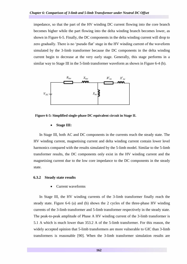
Figure 6-5 Simplified single-phase DC equivalent circuit in Stage II 162
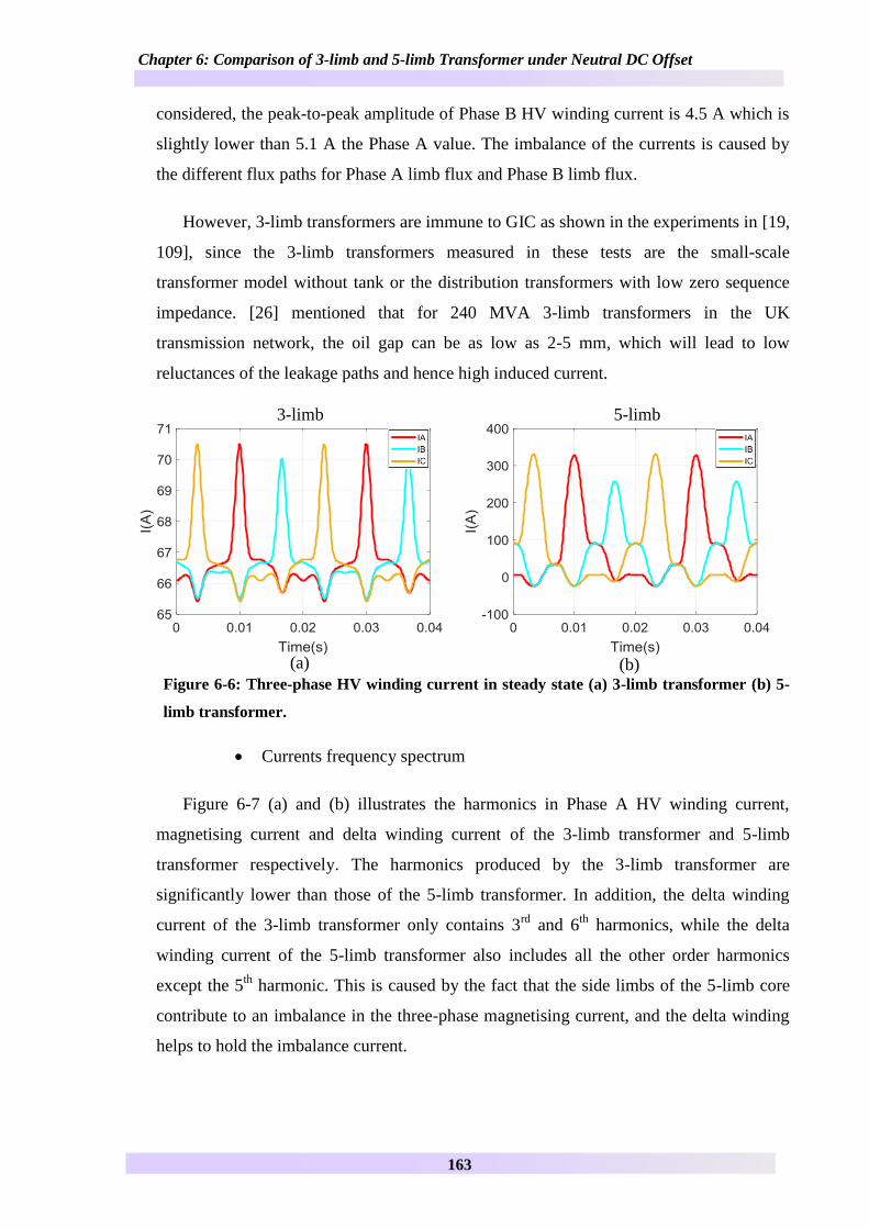
Figure 6-6 Three-phase HV winding current in steady state (a) 3-limb transformer (b) 5-limb
transformer 163
Figure 6-7 Frequency spectrum of Phase A HV winding current magnetising current and
delta winding current in steady state (a) 3-limb transformer (b) 5-limb transformer 164
Figure 6-8 Steady-state winding current and flux densities (a) Phase A HV winding current
Ihv_a magnetising current Ima of 3-limb transformer (b) Phase A HV winding current Ihv_a
magnetising current Ima of 5-limb transformer (c) Delta (TV) winding current Itv_a Itv_b Itv_c of
3-limb transformer (d) Delta (TV) winding current Itv_a Itv_b Itv_c of 5-limb transformer (e)
List of Figures
10
flux densities of limbs and tank of 3-limb transformer (f) flux densities of limbs and tank of
5-limb transformer (g) flux densities of yokes and tank of 3-limb transformer (h) flux
densities of yokes and tank of 5-limb transformer 166
Figure 6-9 Flux density frequency spectrum for (a) 3-limb transformer core (b) 5-limb
transformer core (c) 3-limb transformer tank (d) 5-limb transformer tank 167
Figure 6-10 Peak-to-peak amplitude of Phase A HV winding current against neutral DC
current for (a) 3-limb and 5-limb transformers ranging from 0 A to 300 A (b) 3-limb
transformer ranging from 0 A to 600 A 169
Figure 6-11 Phase A 2nd
harmonic in HV winding current simulated by (a) 3-limb
transformer over 30 s (b) 5-limb transformer over 30 s (c) 5-limb transformer over 60 s 170
Figure 6-12 Phase A limb DC flux density simulated by (a) 3-limb transformer over 30 s (b)
5-limb transformer over 30 s (c) 5-limb transformer over 60 s 171
Figure 6-13 Phase A HV winding current of 3-limb transformer and 5-limb transformer
simulated by Hybrid model 172
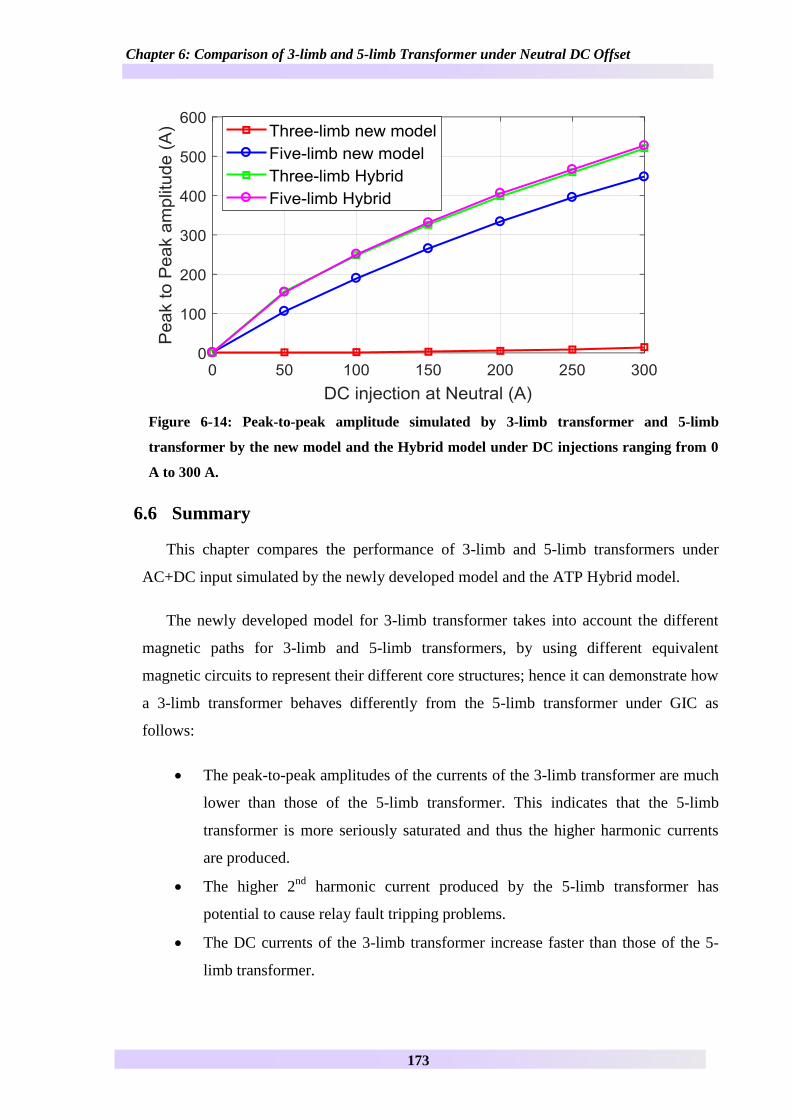
Figure 6-14 Peak-to-peak amplitude simulated by 3-limb transformer and 5-limb transformer
by the new model and the Hybrid model under DC injections ranging from 0 A to 300 A 173
Figure 7-1 Currents and DC components calculated by frequency spectrum (a) with delta
winding (b) without delta winding 176
Figure 7-2 Phase B limb DC flux density for the transformer with a delta winding and the
transformer without a delta winding 177
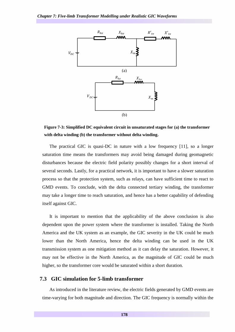
Figure 7-3 Simplified DC equivalent circuit in unsaturated stages for (a) the transformer with
delta winding (b) the transformer without delta winding 178
Figure 7-4 DC voltage provided at neutral 180
Figure 7-5 DC components in Phase A and Phase B HV winding current under a time
varying DC voltage input 181
Figure 7-6 2nd
harmonics in Phase A and Phase B HV winding current under a time varying
DC voltage input 182
Figure 7-7 DC flux densities in Phase A and Phase B limb under a time varying DC voltage
input 183
Figure 7-8 DC voltage provided at neutral with reversed step 184
Figure 7-9 DC components in Phase A and Phase B HV winding current under two different
time varying DC voltage inputs 185
Figure 7-10 2nd
harmonics in Phase A and Phase B HV winding current under two different
time varying DC voltage inputs 185
Figure 7-11 DC flux densities in Phase A and Phase B limb under two different time varying
DC voltage inputs 186
Figure 7-12 (a) DC voltage input at neutral (b) DC components in Phase A and Phase B HV
winding current (c) 2nd
harmonic in Phase A and Phase B HV winding current (d) DC flux
density in Phase A and Phase B limb 187
Figure 7-13 Phase B HV winding current magnetising current load current and delta
winding current referred to the HV side with 95 power factor full load in steady state 189
Figure 7-14 Comparison between Phase B results in the full load and no load (a) HV
winding current (b) Magnetising current (c) Delta winding current (d) Limb flux density 190
List of Figures
11
FigureA 1 BCTRAN input interface for 400 kV transformer 206
FigureA 2 STC model input interface for 400 kV transformer 206
FigureA 3 Hybrid model input interface for 400 kV transformer 207
FigureA4 Power losses caused by nominal AC and DC flux 213
FigureA5 Error of core losses curve fitting 213
FigureA6 Transformer flitch plate temperature rise by Finnish Grid measurement and the
power loss at each step [13] 215
List of Tables
12
List of Tables
Table 3-1 List of solar cycles from Cycle 18 to Cycle 24 [49] 45
Table 3-2 Scale of geomagnetic disturbance relevant Kp index and average days for each
scale at each solar cycle 46
Table 3-3 Risks of GIC in different transformer structures [26] 53
Table 3-4 Historical GIC events in North America 55
Table 3-5 Historical GIC events in UK 56
Table 3-6 Historical GIC events in the rest of the world 57
Table 3-7 Advantages and Disadvantages of GIC mitigation devices 59
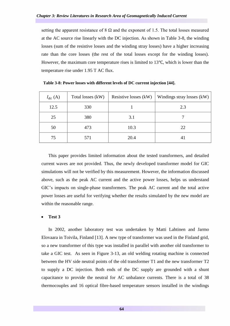
Table 3-8 Power losses with different levels of DC current injection [44] 64
Table 3-9 Advantages and disadvantages of ATP models 76
Table 3-10 Bus bar voltage for north-south direction and east-west direction [21] 78
Table 3-11 GIC current at each substation for Northward direction and Eastward direction
[21] 79
Table 4-1 Required parameters for three widely used ATP transformer models 85
Table 4-2 Transformer basic information to be applied in simulation 86
Table 4-3 Average short circuit test report data for 5-limb transformers in Southwest UK
transmission system 87
Table 4-4 Average open circuit test report data for 5-limb transformers in Southwest UK
transmission system 87
Table 4-5 Core length and cross-sectional area ratio of a 400 kV UK transformer 88
Table 4-6 Transformer basic information to be applied in simulation 103
Table 4-7 Transformer dimensions of the 5-limb transformer applied in the equivalent
magnetic circuit 104
Table 5-1 Severities of core and tank dimensions affecting GIC simulation results 154
Table 6-1 Transformer basic information applied in simulation for 3-limb transformer 157
Table 6-2 Tank and core size of the artificial 400 kV 3-limb transformer 158
Table 7-1 Comparison between the simulation results under no load and full load 191
TableA1 Iteration calculation process of bisection method 210
List of Abbreviations
13
List of Abbreviations
ATPEMTP Alternative Transient ProgramElectromagnetic Transients Program
AC Alternating Current
CGO Conventional Grain-oriented Steels
DC Direct Current
EMF Electromotive Force
EMR Ministry of Energy Mines and Resources
FEM Finite Element Method
GIC Geomagnetically Induced Current
GMD Geomagnetic Disturbances
GSU Generator Step-up
HGO High Permeability Grain-oriented Steels
HV High Voltage
LV Low Voltage
MMF Magnetomotive Force
NG National Grid Electricity Transmission plc
NOAA National Oceanic and Atmospheric Administration
RMS Root Mean Square
SESC Space Environmental Service Centre
SSN Smoothed Sunspot Number
STC Saturable Transformer Component
SVC Static VAR Compensator
List of Symbols
14
List of Symbols
Symbol Meaning Unit
[119860] Cross-section area (m2)
119860119886119906119903119900119903119886 Vector potential of aurora-zone current (A)
[119860119886 119860119887 119860119888] Cross-section area of main limbs (m2)
[119860119897] Cross-section area of side limbs [1198601198971 1198601198972] (m2)
[119860119900] Cross-section area of oil gaps (m2)
[1198601199001 1198601199002 1198601199003 1198601199004 1198601199005]
[119860119905] Cross-section area of tank paths (m2)
[1198601199051 1198601199052 1198601199053 1198601199054 1198601199055]
[119860119910] Cross-section area of yokes (m2)
[1198601199101 1198601199102 1198601199103 1198601199104]
119861 Magnetic flux density (T)
[119861119886 119861119887 119861119888] Flux density at main limbs (T)
[119861119897] Flux density at side limbs [1198611198971 1198611198972] (T)
[119861119900] Flux density at oil gaps [1198611199001 1198611199002 1198611199003 1198611199004 1198611199005] (T)
[119861119905] Flux density at tank paths[1198611199051 1198611199052 1198611199053 1198611199054 1198611199055] (T)
[119861119910] Flux density at yokes [1198611199101 1198611199102 1198611199103 1198611199104] (T)
119889 Thickness of laminations (m)
119864 Electric field (Vkm)
119864119864 Electric field in eastward (Vkm)
119864119873 Electric field in northward (Vkm)
1198641 Electromotive force on HV side (V)
119891 Frequency (Hz)
119866minus1 Inverse admittance (Ω-1
)
119867 Magnetic field intensity (Am)
[119867119886 119867119887 119867119888] Magnetic field intensity at main limbs (Am)
[119867119897] Magnetic field intensity at side limbs [1198671198971 1198671198972] (Am)
[119867119900] Magnetic field intensity at oil gaps (Am)
[1198671199001 1198671199002 1198671199003 1198671199004 1198671199005]
[119867119905] Magnetic field intensity at tank paths (Am)
List of Symbols
15
[1198671199051 1198671199052 1198671199053 1198671199054 1198671199055]
[119867119910] Magnetic field intensity at yokes (Am)
[1198671199101 1198671199102 1198671199103 1198671199104]
119868119888 Current supplying core loss (A)
119868119889119888 DC current (A)
119868ℎ119907 HV winding current (A)
119868119897119907prime LV winding current referred to HV side (A)
119868119898 Magnetising current (A)
119868119905119907prime TV winding current referred to HV side (A)
1198680 No-load current (A)
119870119901 Geomagnetic intensity NA
119896 Reluctance (AWb)
119896119886 Anomalous loss constant NA
119896ℎ Hysteresis loss constant NA
119896119897119900119904119904 Coefficient of reactive power loss MVarA
119871ℎ119907 HV winding inductance (mH)
119871119897119907prime LV winding inductance referred to HV side (mH)
119871119898 Core inductance (mH)
119871119905119907prime TV winding inductance referred to HV side (mH)
119897 Distance between substations (km)
[119897119886 119861119887 119861119888] Length of main limbs (m)
119897119864 Distance between substations in eastward (km)
[119897119897] Length of side limbs [1198971198971 1198971198972] (m)
119897119897119900119900119901 Magnetic path length for all loops (m)
119897119873 Distance between substations in northward (km)
[119897119900] Length of oil gaps [1198971199001 1198971199002 1198971199003 1198971199004 1198971199005] (m)
[119897119905] Length of tank paths [1198971199051 1198971199052 1198971199053 1198971199054 1198971199055] (m)
[119897119910] Length of yokes [1198971199101 1198971199102 1198971199103 1198971199104] (m)
119873 Winding turn number NA
119899 Stein exponent NA
119875119886119899119900119898119886119897119900119906119904 Anomalous loss (Wkg)
List of Symbols
16
119875119888119900119903119890 Core loss (Wkg)
119875119890119889119889119910 Eddy current loss (Wkg)
119875ℎ119910119904119905119890119903119890119904119894119904 Hysteresis loss (Wkg)
119877119888 Core resistance (Ω)
119877ℎ119907 HV winding resistance (Ω)
119877119897119907prime LV winding resistance referred to HV side (Ω)
119877119905119907prime TV winding resistance referred to HV side (Ω)
119878119887 Power base (VA)
119881119860119862 AC voltage source matrix (V)
119881119863119862 DC voltage source (V)
119881ℎ119907 HV wide terminal voltage (V)
119881119871119871 Rated line voltage (kV)
119881119897119907prime LV wide terminal voltage referred to HV side (V)
Δ119881 Voltage drop between substations (V)
119885119897119900119886119889 Load impedance (Ω)
120033 Reluctance (AWb)
120567 Magnetic flux (Wb)
120567119894119899119894119905119894119886119897 Limb initial magnetic flux (Wb)
120567119901119890119886119896 Magnitude of limb nominal flux (Wb)
120588 Steel lamination resistivity (Ωm)
Abstract
17
Abstract
During the peak years of solar activity the magnetic field held by the solar wind has an
impact on the Earthrsquos magnetic field and induce an electric field on the Earthrsquos surface The
Geomagnetically Induced Current (GIC) is generated between two neutral points of
transformers The GIC can do severe harm to a power system including to its transformers
The worst GIC event caused a power system blackout for several hours in Quebec in 1989
The research aims to build a representative model of core saturation and carry out simulation
studies to understand the performance of transformer cores in the high flux density region
This in turn helps to identify the design features that need to be taken into account when
assessing the capability of a transformer to withstand over-excitation
ATP is a kind of user-maintained software so it allows self-developed code to be added into
the software package The results simulated by the existing ATP models are inaccurate
compared to the measured results In addition the existing models cannot provide flux
distribution results so it is difficult to understand the process of how the core is pushed into
the deep saturation region by DC offset
A new model is developed to include the equivalent electric and magnetic circuit
representations taking flux leakage in particular into consideration The flux leakage paths
are composed of the oil gaps and tank in series This model is validated by the consistency
shown between the measured and simulated HV winding currents of a 5-limb transformer
The peaks of magnetising currents are identified with the peaks of magnetic flux which
saturate the core
The model can identify the design features such as the core structure dimension of flux
leakage paths and winding impedance that need to be taken into account when assessing the
capability of a transformer to withstand over-excitation A 3-limb model and a 5-limb core
model are built to assess the susceptibility to GIC for different core types in high flux density
region The delta winding plays a role in holding the 3rd
harmonics and unbalanced current
generated by core saturation and in delaying the core saturation Lastly Transformers are
simulated under realistic GIC waveforms for situations with and without load
The new model is expected to be coded into ATP to conduct a GIC study for a power system
Declaration
18
Declaration
I declare that no portion of the work referred to in the thesis has been submitted in
support of an application for another degree or qualification of this or any other
university or other institute of learning
Copyright Statement
19
Copyright Statement
(i) The author of this thesis (including any appendices andor schedules to this thesis)
owns certain copyright or related rights in it (the ldquoCopyrightrdquo) and she has given The
University of Manchester certain rights to use such Copyright including for
administrative purposes
(ii) Copies of this thesis either in full or in extracts and whether in hard or electronic
copy may be made only in accordance with the Copyright Designs and Patents Act 1988
(as amended) and regulations issued under it or where appropriate in accordance with
licensing agreements which the University has from time to time This page must form
part of any such copies made
(iii) The ownership of certain Copyright patents designs trade marks and other
intellectual property (the ldquoIntellectual Propertyrdquo) and any reproductions of copyright
works in the thesis for example graphs and tables (ldquoReproductionsrdquo) which may be
described in this thesis may not be owned by the author and may be owned by third
parties Such Intellectual Property and Reproductions cannot and must not be made
available for use without the prior written permission of the owner(s) of the relevant
Intellectual Property andor Reproductions
(iv) Further information on the conditions under which disclosure publication and
commercialisation of this thesis the Copyright and any Intellectual Property andor
Reproductions described in it may take place is available in the University IP Policy (see
httpwwwcampusmanchesteracukmedialibrarypoliciesintellectual-propertypdf) in any
relevant Thesis restriction declarations deposited in the University Library The
University Libraryrsquos regulations (see httpwwwmanchesteracuklibraryaboutusregulations)
and in The Universityrsquos policy on presentation of Theses
Acknowledgement
20
Acknowledgement
First of all I would like to express sincere gratitude to Professor Zhongdong Wang My
PhD research has greatly benefited from her patience motivation and immense
knowledge She has been my supervisor since I was an undergraduate student at the
University of Manchester She has given me extensive personal and professional
guidance and taught me a great deal about both scientific research and life in general It is
a great honour for me to have such an outstanding and kind supervisor
My sincere thanks also go to my co-supervisor Professor Peter Crossley and Dr Qiang
Liu I would particularly like to thank Dr Liu for his selfless support and valuable advice
I am especially indebted to Professor Paul Jarman and Dr Philip Anderson for their
technical support and invaluable suggestions
I greatly appreciate the financial scholarship from National Grid and the University of
Manchester that has supported my PhD research
I am very fortunate to have spent four memorable years at the University of Manchester
to complete my PhD study My lovely colleagues in the transformer research group have
made me feel at home I would like to express my heartfelt gratitude to them for their
company and friendship
Last but not least I would like to thank my parents and my grandparents whose love and
guidance are with me in whatever I pursue Their unconditional support and
encouragement always drive me forward
Chapter 1 Introduction
21
Chapter 1 Introduction
11 Background
Transformer 111
Transformers are widely used in electrical power systems to step up or step down
voltages between different parts of the network The voltage step up by a transformer
contributes to a reduction in power losses in transmission lines while step-down
transformers convert electric energy to a voltage level accessible by both industrial and
household users
A transformer is electrical-magnetic equipment involving two closely magnetically
coupled windings as the electrical circuit where electrical energy is transmitted from one
voltage level to the other An ideal transformer will neither store nor dissipate energy
[1] Perfect magnetic coupling contributes to infinite core magnetic permeability and zero
magnetomotive force In reality the core steel permeability cannot be infinite and
therefore it is inevitable that a magnetomotive force is produced and hence a magnetising
current too A transformer is designed in such a way that the magnetising current
normally remains at a low level when a transformer is operated at its nominal voltage and
frequency This is achieved by utilising the electrical steelrsquos B-H curve characteristics and
selecting the nominal operating point around the knee point It should be also noted that
core permeability has increased significantly since the invention of power transformers
with the application of optimized electrical steel material
Transformers are mainly divided into two categories shell type and core type
depending on the physical arrangement of the magnetic and electrical circuits Core type
transformers are more popular worldwide than shell type transformers which exist in
several countries such as the United States and Japan Three-phase transformers are more
economical than three single-phase transformer banks due to the shared magnetic circuit
the shared tank and other design features so the majority of power transformers are three-
phase transformers Transformer banks tend to be used for high power rating transformers
(eg generator transformer exceeding 600 MVA) or due to transportation restrictions or
reliability considerations
Chapter 1 Introduction
22
Historically power transformers just like the power systems were developed
gradually from low voltage to high voltage rating For core type transformers 3-limb
transformers are almost the only type used in distribution systems With the increase in
power rating 5-limb core has become an optional design for large transmission
transformers since this type of design reduces the height of core and tank making it
easier to transport However 3-limb transformers without outer limbs save core material
and reduce core losses as compared to 5-limb transformers
Auto-connected transformer design aims to save winding and core material and to
reduce the transformer size and the construction cost [2] therefore it is popular in
transmission interbus transformers where the voltage ratio between two windings is
generally less than 31 Installation of a delta winding is recommended in three-phase
auto-transformers because it can provide a low impedance path for triplen harmonics so
that the system is potentially less impacted by the harmonics In addition a delta winding
holds the unbalanced current produced by the unbalance load Lastly tertiary windings
are also sometimes used to connect reactors at some substations to control voltage as well
as reactive power
UK power system network 112
Figure 1-1 shows the schematic diagram of the UK network [3] The transmission
network in the UK normally refers to the part operating above 132 kV while the
maximum voltage level in the UK network is 400 kV In England and Whales the
transmission network is operated by National Grid Electricity Transmission plc [4]
while Scottish Power Transmission Limited operates the network for southern Scotland
and Scottish Hydro Electric Transmission plc for northern Scotland and the Scottish
islands groups [5]
According to the National Grid database in 2010 among the 950 transmission
transformers the percentages of the 400275 kV 400132 kV 275132 kV and 27533 kV
transformers were 148 278 338 and 68 respectively According to the data in
National Grid Electricity Ten Year Statement the 400275 kV and 275132 kV
transformers are mainly located in densely-populated areas or near to large industrial
loads such as London Birmingham Cardiff Manchester Edinburgh and Glasgow
Naturally a higher nominal voltage is associated with a higher power rating of a power
Chapter 1 Introduction
23
transformer Among the 400275 kV transformers 436 of the transformers are
specified at the nominal power rating of 750 MVA while the transformers rated at 1000
MVA and 500 MVA account for 307 and 164 The remaining 400275 kV
transformers operate at 900 MVA 950 MVA and 1100 MVA 951 of the 400132 kV
transformers are specified at a nominal power rating of 240 MVA while the remaining
400132 kV transformers have a power rating of 120 MVA 220 MVA 276 MVA or 288
MVA Moreover the power rating of the 275 kV (HV side) transformers will normally
not exceed 240 MVA Regarding the 275132 kV transformers the majority of the them
operate at 120 MVA 180 MVA and 240 MVA (190 536 and 249) while the
power rating of the rest are 150 MVA and 155 MVA
Figure 1-1 Schematic diagram of typical UK network [3]
All the NG transmission interbus transformers (400275 kV 400132 kV and 275132
kV) are auto (Y-a-d) connected as the turn ratios between the HV side and LV side of the
NG transmission transformers are lower than or close to 31 so autotransformers are
more economical than two-winding transformers In addition 13 kV delta connected
tertiary windings are broadly used in NG transmission interbus transformers
Generator
transformer
Generator
400275 kV
transformer
400 kV transmission network
275 kV
transmission
network 275132 kV
transformer
400132 kV
transformer
Transmission network
132 kV distribution network
13233 kV
transformer
3311 kV
transformer
11 kV415 V
transformer
Industrial use
Industrial use
Industrial use
Users
Distribution network
33 kV distribution network
33 kV distribution network
11 kV distribution network
Chapter 1 Introduction
24
In the National Grid database a simple statistic shows that the number of 3-limb
transformers is greater than 5-limb transformers Taking 32 interbus transformers in the
Southwest England NG Peninsula system as an example 16 transformers are of the 3-
limb core type and 8 transformers are of the 5-limb core type For the other 8
transformers it is difficult to ascertain their core types due to a lack of evidence
Using the transformer data in the National Grid Database Figure 1-2 displays the
magnetising currents of the National Grid 40027513 kV 1000 MVA transformers
manufactured before the 1990s and after the 1990s respectively The statistics indicate
that the transformers produced after the 1990s normally have lower magnetising currents
(on average 0013 pu) than the ones built before the 1990s (on average 0053 pu) In
addition an imbalance is found in the three-phase magnetising currents from the same
family which could be caused by the unsymmetrical design of three-phase flux paths for
three-phase transformers
Figure 1-2 Magnetising current for 40027513 kV 1000 MVA transformers manufactured
before the 1990s and after the 1990s in National Grid system
The reason why transformers have low magnetising currents under normal operation
is that the core operating point is always limited below the knee point which expects to
retain the core linearity to avoid excessive harmonic currents and power losses However
if a transformer suffers external interference such as inrush current ferroresonance or
Geomagnetically Induced Current (GIC) the transformer core will work beyond the knee
point and the magnetising current will be severely distorted
Before 1990s After 1990s
Phase A 00493 00118
Phase B 00487 00120
Phase C 00610 00157
000
002
004
006
008
010
Magn
etis
ing c
urr
ent
()
Chapter 1 Introduction
25
A brief description of the three power system transient phenomena which involve the
core characteristics and which are normally hidden in a normal 50 Hz operation is given
here Firstly inrush current is caused by the non-linear characteristics of transformer core
When a transformer is energized the transformer core tends to enter the non-linear
operation area due to the switching angle and the residual flux retained in the core since
last switch-off and hence an excessive magnetising current containing rich harmonics
and great power losses will be produced [6] The magnitude of the inrush current could be
several times the rated current [7] Secondly ferroresonance refers to the non-linear
resonance resulting from the saturated core inductances and the system capacitance
during the opening switch operation After system capacitance is cancelled with core
inductance the energy stored in the series capacitance leads to an overvoltage problem
which pushes the transformer core into the saturation area and hence rich harmonics and
excessive power losses are generated The magnitude of the overvoltage could reach 15
times the nominal voltage [8] Lastly during solar storms Geomagnetically Induced
Current will be generated on the Earthrsquos surface which pushes the transformer core into
the saturation area gradually [9] In conclusion transformers are vulnerable in these
abnormal situations so it is necessary to investigate these issues to provide a
comprehensive protection for transformers
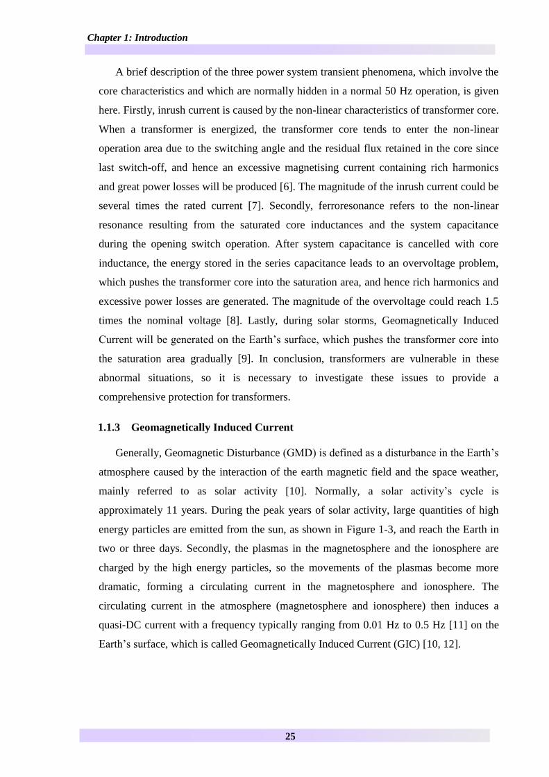
Geomagnetically Induced Current 113
Generally Geomagnetic Disturbance (GMD) is defined as a disturbance in the Earthrsquos
atmosphere caused by the interaction of the earth magnetic field and the space weather
mainly referred to as solar activity [10] Normally a solar activityrsquos cycle is
approximately 11 years During the peak years of solar activity large quantities of high
energy particles are emitted from the sun as shown in Figure 1-3 and reach the Earth in
two or three days Secondly the plasmas in the magnetosphere and the ionosphere are
charged by the high energy particles so the movements of the plasmas become more
dramatic forming a circulating current in the magnetosphere and ionosphere The
circulating current in the atmosphere (magnetosphere and ionosphere) then induces a
quasi-DC current with a frequency typically ranging from 001 Hz to 05 Hz [11] on the
Earthrsquos surface which is called Geomagnetically Induced Current (GIC) [10 12]
Chapter 1 Introduction
26
Figure 1-3 Effects of geomagnetic disturbances on Earthrsquos surface magnetic field [10]
GIC has great effects on power systems [13 14] During GMD events the quasi-DC
current flows into the power system via the neutral points of two transformers The
neutral quasi-DC current tends to push the transformer core into the deep saturation area
which drives the magnetising currents to a higher magnitude containing greater
harmonics The excessive current and the deep saturated core lead to an increase in
copper losses core losses and reactive power consumption Meanwhile the excessive
voltage drop across the transformer with the saturated core leads to low power delivery
efficiency [14]
The abnormality of a transformerrsquos operation during GMD events will also influence
the other equipment in the power system such as generators relays and shunt capacitor
banks Generally speaking generators are not exposed to GIC directly due to the D-Y
winding connection for step-up transformers However the voltage drop and the
excessive harmonics produced by the GIC effects in transmission systems could influence
generators and result in excessive heating and stimulation of mechanical vibrations in
generators [15] During severe GIC events abnormal relay tripping could be triggered by
high peak currents or rich harmonics in the power system Moreover the overcurrent
relays which aim to protect the shunt capacitor banks are susceptible to harmonic
currents because capacitors show low impedance to harmonics [16]
For this reason it is necessary to understand how GIC will impact transformers and
power systems so that precautions can be taken before equipment in power system is
Sun Earth
High energy
particles
Chapter 1 Introduction
27
damaged This thesis mainly focuses on the impacts of Geomagnetically Induced Current
on power transformers
Solar activity also has negative effects on other man-made systems such as
communication systems and pipelines
Firstly the radiation produced by the solar storms causes the ionization of the
ionosphere which changes the radio wave propagation behaviour in the atmosphere [15]
In addition the high energy particles generated during solar storms perturb the Earthrsquos
magnetic field which results in disturbances to wireline facilities [15] In 1847 Varley
observed the telegraph line was interrupted by Earthrsquos current in Great Britain [9]
Secondly GIC can accelerate the corrosion of steel-made pipelines in that they
contain high pressure liquid or gas To prevent corrosion of the pipelines due to chemicals
or other factors the pipeline always has a protection coat In case the coat is damaged for
natural reasons a negative potential is supplied along the pipeline to provide protection
from corrosion However during a GMD event this protection could be less effective
making the pipelines susceptible to corrosion and the reducing their service life [17] For
example if a pipeline is exposed to a 05 V potential change (Equivalent to Kp=5 Kp is
the GMD strength and will be introduced in Chapter 3) due to a GMD event the
corrosion rate will be 006 and 0152 mmyear for GMD periods of 001 and 1 h
respectively both exceeding 0025 mmyear which is generally considered as the
acceptable corrosion rate [18]
Motivations 114
Currently the research on GIC studies can be divided into two categories
experiments and simulations Experiments can provide reliable results however due to
the fact that only a limited number of transformers can be used in GIC tests and limited
tests can be undertaken for each tested transformer experimental measurements cannot be
widely used in investigating GIC issues In order to overcome the weakness of the
measurements the simulations both for large scale power systems and for individual
transformers have become popular in the GIC investigation
A laboratory test was undertaken by Matti Lahtinen in Toivila Finland [13] Two
40012021 kV transformers were set in parallel with an old rotating welding machine
Chapter 1 Introduction
28
connected between their neutral points to feed DC injection up to 200 A 38
thermocouples and 16 optical fibre-base temperature sensors are inserted into one of the
transformers to record the temperature data In addition Nobuo Takasu and Tetsuo Oshi
compared the performances of the transformers with three different core types under
AC+DC input in 1993 [19] In the test the transformers are shrunk to 120 of the original
dimension and the metallic tanks are not added to the transformers On the one hand
these experiments can provide the test results for specific transformers under particular
voltage supply but the measurement results cannot be applied to the other transformers
Therefore it is essential to undertake simulation work to investigate various types of
transformers On the other hand the accuracy of the simulated results can be verified by
comparing them with the measured results
The large scale power system simulation applies the full-node linear resistance
methods [20 21] which simplifies the transformers transmission lines and neutral
grounds into linear resistances In this way the transient process is ignored to save
computation time and improve simulation efficiency However the reactive power losses
generated by a GIC event at each transformer need to be estimated by empirical equations
that rely simply on the terminal DC voltage and the GIC level where the empirical
parameters remain to be tested and verified for all the occasions [22 23] In this way this
method can efficiently evaluate the GIC severities for transformers at different locations
which could help the operators analyse the GIC risks and plan for precautions It is
apparent that this method sacrifices the accuracy of simulation results because the
transient characteristics of the equipment in power systems are completely ignored The
disadvantage is of course that the results are still a controversial issue for this method
because the precision of the simulation relies heavily on the parameters used in the
empirical equations In addition this method cannot distinguish the GICrsquos impacts on
different types of transformers
Taking the nonlinear characteristics into consideration researchers develop various
transformer models to conduct GIC transient simulations for individual transformers or
small-scale power systems [24-26] If the transformer saturation characteristics are
properly described the transient simulation will provide a better view on how the DC
neutral input saturates the transformers EMTP is one of the software platforms which
enables the transient simulation by using either internal or external transformer models
Chapter 1 Introduction
29
EMTP or EMTDC is the suite of commercialised software [7 27] which includes
EMTP-RV MT-EMTP EMTP-ATP and PSCAD-EMTDC EMTP-ATP (referred as
ATP) is a kind of user-maintained software so it allows self-developed code to be added
into the software package There are three transformer models widely used in ATP the
BCTRAN model the Saturable Transformer Component (STC) model and the Hybrid
model The Hybrid model is applicable in simulating GMD event because it considers
both the core topology and the core non-linear saturation effects [28] although the
simulation results cannot exactly match the measurement results
Currently there is no accurate model for the magnetic circuit of a transformer under
high induction conditions limiting the conclusions about the relationship between GIC
and the level of damage a transformer may receive from a GIC This inability appears to
be general throughout the transformer industry and represents a significant gap in
knowledge This gap does not seem significant to transformer manufacturers because
during routine factory tests the core of a transformer is operated below or around the
maximum operational flux limits For a utility conservative assumptions about core
saturation have therefore had to be adopted Failure to accurately analyse these system
events induced core saturation conditions leads either to excessive capital cost in
increasing core dimensions or potential failure in service due to the heating of the
magnetic circuit and other steel parts in the transformers or reactors
In conclusion it is necessary to build a new model that enables the performance of
transformer cores to be modelled in the high flux density region by producing a viable
algorithm to represent transformer magnetic circuits under deep saturation Also the
model enables the identification of design features that must be considered when
assessing the capability of a transformer to withstand over-excitation
12 Objective of research
This project aims to investigate the GICrsquos impacts on transformers and power systems
in transient The work can be divided two steps Firstly the accuracy of the existing ATP
models for simulating core half-cycle saturation effect will be verified However none of
the existing models can accurately present the core saturation effect and key information
For example the flux distribution and the magnetising current are unavailable in ATP so
it seems a new model is required for the GIC transient study Secondly a new transformer
which combines the electric circuit and magnetic circuit is built for a better
Chapter 1 Introduction
30
understanding of transformer performance under AC and DC excitation because it is
accessible to the flux distribution and magnetising current By implementing this model
various transformer design features can be identified when assessing the transformer
vulnerability to GIC Furthermore this model can be applied to investigate the impacts of
the practical GIC injection and the load characteristics to the simulation results Thirdly a
GIC study is conducted for part of the UK transmission system by using ATP and the
new model is expected to replace the ATP model in the future study The specific
objectives are listed as follows
Examination of the existing transient simulation capability
Understand the working principles of the existing ATP models and validate
the models under AC+DC input The simulation results are to be compared
with the measurement results
Development and application of the new transformer model
Develop a new model which incorporates the equivalent electric and magnetic
circuits and takes the core saturation effect and the tank leakage flux paths into
consideration The model will be validated under AC+DC input by comparing
it to the measurement results
Understand the transient process before the transformer reaches the steady
state Analyse the flux distribution in the core and the tank corresponding to
the magnetising current in the steady state which makes it possible to evaluate
the most vulnerable part in a transformer that suffers overheating problems
Identify the designing features that need to be taken into account when
assessing the capability of a transformer to withstand over-excitation such as
the various dimensions of the core and tank the core type the winding type
(including a delta winding or not) and the winding impedance
Investigate the performance of transformers under different practical time
varying neutral injections
Explore the impacts of the load characteristics on transformer operation state
under neutral DC injection
GIC simulation for part of the UK transmission system
Build part of the UK transmission system in ATP by using the existing ATP
models Give a case study to investigate the influences from the real GMD
injection on the power system
Chapter 1 Introduction
31
In the future the newly developed model is expected to be coded into ATP to
conduct a power system level study for GIC
13 Outline of the thesis
This thesis contains eight chapters which are briefly summarized below
Chapter 1 Introduction
This chapter gives a general introduction of transformers and Geomagnetically
Induced Current The objectives and the scope of the research are also presented
Chapter 2 Overview of Transformer Core and Winding
This chapter introduces the key components of transformers the core and the winding
Firstly the transformer core is described in terms of the core configuration core steel and
core losses Secondly the winding structures widely used in the UK transformers are
discussed Lastly this chapter explains the transformer equivalent circuit
Chapter 3 Review Literatures in Research Area of Geomagnetically Induced
Current
This chapter provides an overview of Geomagnetically induced current from several
aspects First of all it introduces how GIC is produced on the Earthrsquos surface and the
factors determining the GIC level Following that the GICrsquos impacts on power system
networks together with the historical GIC events are given Then the GIC mitigation
devices are reviewed Researchers have carried out GIC investigation through either
experiments or simulations in recent years This chapter conducts two categories of
simulation methods which are the non-linear model simulation for individual
transformers and the equivalent full-node simplified resistance method for system level
study together with three experimental cases aiding to validate the modelling accuracy
of the transformer models
Chapter 4 Development of Transformer Models for GIC Simulation Studies
This chapter firstly compares the results measured by Finnish Grid and the simulation
results generated by three ATP models which are the BCTRAN model the STC model
and the Hybrid model to determine their suitability for GIC simulation Secondly a new
Chapter 1 Introduction
32
model that represents the equivalent electric and magnetic circuits of a transformer is
developed based on material properties and physical dimension parameters The model
has an advantage that the leakage flux paths composed of the tank and oil gaps are
adequately modelled A 400 kV 5-limb transformer is given as an example to validate the
model under AC+DC input Many parameters interested such as the flux distribution the
current flow insides a delta connected winding and magnetising current can be extracted
to aid the understanding
Chapter 5 Sensitivity Study for New Model Parameters
This chapter conducts sensitivity studies on the structure of the transformer core
parameters of the tank-oil paths and winding impedance since it is necessary to
understand how sensitive each parameter used in the simulation impacts the results The
feature of the core structure looks into the cross-sectional area ratio between the yokes
and limbs The features that make up the tank-oil paths are the equivalent tank length the
tank area the oil gap length and the oil gap area The last part concentrates on the
resistance and leakage inductance of the HV winding and the delta winding
Chapter 6 Comparison of 3-limb and 5-limb Transformer under Neutral DC Offset
This chapter firstly introduces the newly developed 3-limb model and compares the
simulation results of a 3-limb transformer and a 5-limb transformer under AC+DC input
to prove the conventional concept that 5-limb transformers are more vulnerable to a
neutral DC offset Then the 3-limb transformer and 5-limb transformer are supplied by
various levels of neutral DC offset to investigate the relationship between the induced
current amplitude and the neutral DC offset level Lastly the 3-limb transformer is also
simulated by the Hybrid model and the simulation results are compared to those of the
new model
Chapter 7 Five-limb Transformer Modelling under Realistic GIC Waveforms
In this chapter the GIC transient simulation studies are conducted on the 5-limb
transformer as 5-limb transformers are more susceptible to the neutral DC input than 3-
limb transformers This chapter starts with a study carried out to show the effect of
tertiary delta-connected winding on time constant of saturation It is followed by the
Chapter 1 Introduction
33
simulation of the 5-limb model under practical neutral time varying injection Lastly the
5-limb transformer simulation results with full load situation are also provided
Chapter 8 Conclusion and Future Work
This chapter summarises the key findings in the research and gives recommendations
for future research
Chapter 2 Overview of Transformer Core and Winding
34
Chapter 2 Overview of Transformer Core
and Winding
21 Overview
Proposed in 1831 transformers are based on Faradayrsquos law of induction to transfer
electrical energy among the electrical circuits operating at different voltage levels [29]
Nowadays transformers are widely used for the transmission and distribution of electrical
energy in power systems [30 31] Magnetic core and windings are the most important
parts of a power transformer Magnetic core made of ferromagnetic steel with high
magnetic permeability enables electric energy to be transferred through electromagnetic
induction and windings are made of insulated conductors which carry current In this
chapter magnetic core and windings will be discussed separately from configurations
material and losses
22 Transformer core
Core configuration 221
When transformers are classified by core configuration there are mainly two types of
transformers shell type and core type used in the industry Shell type transformers are
not widely manufactured and installed in the world except North America and Japan [3]
ABB produces shell type transformers designed for high power rating and voltage usage
(Unit rating up to 1300 MVA Primary voltage up to 765 kV single or three phases) [32]
Core type transformers are widely used in the UK and many other parts of the world For
this reason this PhD research will mainly focus on core type transformers
In terms of core type transformers both three-phase transformers and three single-
phase transformer banks are broadly applied in power systems However if both types are
available the industry prefers to use a three-phase transformer because the financial cost
of a bank of three single-phase transformers is about 15 times that of a three-phase
transformer for the same MVA [33] In the NG transmission system in England and
Wales most of the transmission transformers are three-phase transformers However
single-phase transformers are still important in power systems as they can be used at the
end of the distribution system in a rural area far from an urban area with low demand [34]
Chapter 2 Overview of Transformer Core and Winding
35
In addition three single-phase transformer banks are used as generator transformers This
design is convenient for transportation (three single-phase transformer can be transported
separately) and minimises the impact of faults [3]
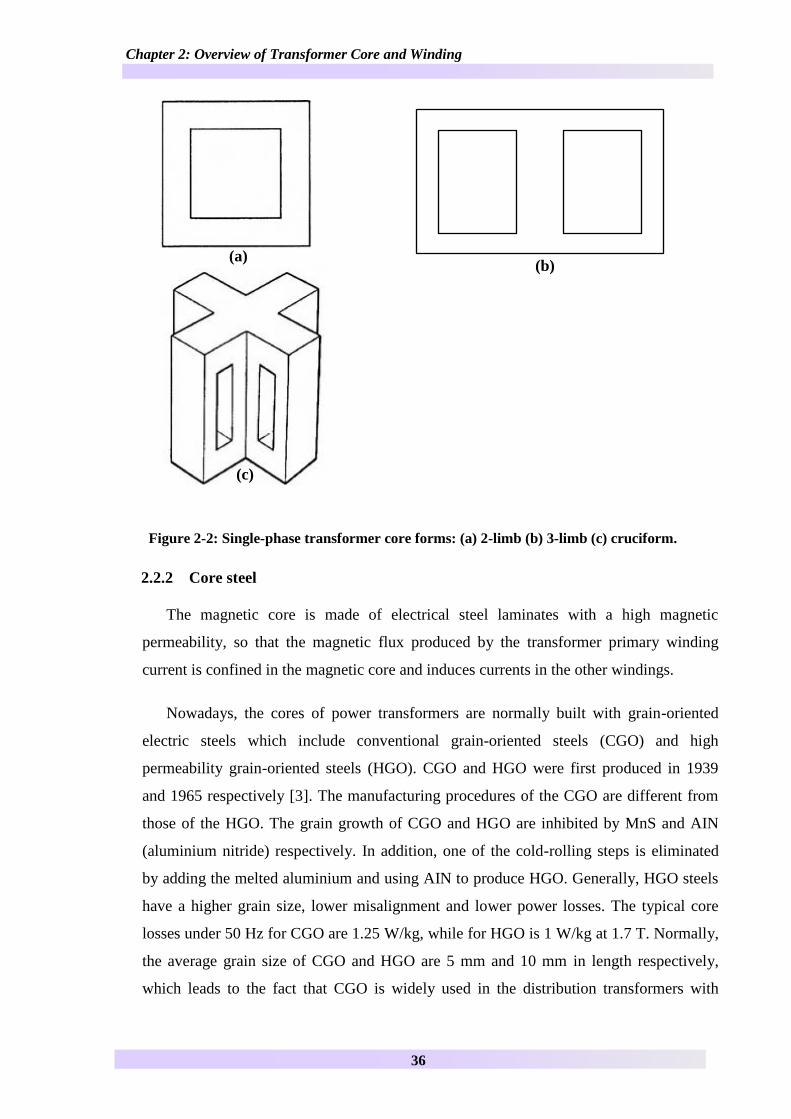
There are two core forms for a three-phase transformer 3-limb core and 5-limb core
as displayed in Figure 2-1 (a) and (b) For a 3-limb core the yoke cross-sectional area is
often equal to that of the limb Three-phase 3-limb core transformers are almost the
unique arrangement in the UK transmission transformers because a 3-limb core saves the
core material as well as reducing core losses In the case of a 5-limb core since the side
limbs can provide valid flux paths the cross-sectional area of the yokes can be reduced by
about 50 so the core height can also be reduced For this reason 5-limb cores are
usually applied in generator transformers or large interbus transformers because the
heights of 5-limb transformers are normally lower than the counterpart of 3-limb
transformers The lower height of a transformer will make transportation more convenient
Figure 2-1 Three-phase transformer core forms (a) 3-limb (b) 5-limb
Figure 2-2 (a) (b) and (c) displays three single-phase transformer core forms For a
single-phase transformer the flux return paths must be provided As shown in Figure 2-2
(a) both limbs are wound and the cross-sectional area of the yoke equals that of the
limbs so the yoke is high for this core form On the other hand for the 3-limb core form
as presented in Figure 2-2 (b) only the middle limb is wound by the windings and the two
side limbs provide the flux return paths so the height of the yoke is reduced In terms of
the cruciform as shown in Figure 2-2 (c) only the middle limb is wound so the height of
the yoke further decreases due to the four side limbs The single-phase distribution
transformers at the rural end always have both-wound 2-limb core since it is not
necessary to reduce the height of a distribution transformer
(b) (a)
Chapter 2 Overview of Transformer Core and Winding
36
Figure 2-2 Single-phase transformer core forms (a) 2-limb (b) 3-limb (c) cruciform
Core steel 222
The magnetic core is made of electrical steel laminates with a high magnetic
permeability so that the magnetic flux produced by the transformer primary winding
current is confined in the magnetic core and induces currents in the other windings
Nowadays the cores of power transformers are normally built with grain-oriented
electric steels which include conventional grain-oriented steels (CGO) and high
permeability grain-oriented steels (HGO) CGO and HGO were first produced in 1939
and 1965 respectively [3] The manufacturing procedures of the CGO are different from
those of the HGO The grain growth of CGO and HGO are inhibited by MnS and AIN
(aluminium nitride) respectively In addition one of the cold-rolling steps is eliminated
by adding the melted aluminium and using AIN to produce HGO Generally HGO steels
have a higher grain size lower misalignment and lower power losses The typical core
losses under 50 Hz for CGO are 125 Wkg while for HGO is 1 Wkg at 17 T Normally
the average grain size of CGO and HGO are 5 mm and 10 mm in length respectively
which leads to the fact that CGO is widely used in the distribution transformers with
(c)
(a) (b)
Chapter 2 Overview of Transformer Core and Winding
37
small size while HGO is applied in the transmission transformers with long limbs and
yokes CGO and HGO have different non-linear characteristics in the saturation region
That is why the material property is one of the key parameters for modelling GIC
phenomena The selection of the grain-oriented material is assessed by total ownership
cost (TOC) which takes into account transformer capital cost the cost of core losses and
winding losses during its lifetime [35]
The magnetising characteristics of the core steel are normally described by B-H
curves Figure 2-3 shows a typical B-H curve for the CGO core steel M140-27S (in EN
10107 Classification-2005 Capital letter M for electrical steel 140 is the number of 100
times the specified value of maximum specific total loss at 50 Hz 17 T 27 represents 100
times of nominal thickness of the product in millimetres S for conventional grain
oriented products) which is also called 27M4 in BS 601 Classification (CGRO Grade is
M4 in power loss and the thickness is 027 mm) Its knee point is about 175 T Normally
transformer core operates in the high induction area below the knee point for example
the generator transformer usually works at maximum flux density 119861119898 of 170 T under
nominal AC voltage Moreover the transmission transformers work in a range from 160
T to 165 T while distribution transformers work around 150 T due to large fluctuations
of loads [3] If the core operates beyond the knee point the permeability of the core
material will decrease rapidly which will further result in serious distortion in the
magnetising current Meanwhile the core losses grow significantly due to the high
magnitude of flux densities
Figure 2-3 Typical B-H curve and knee point of core material M140-27S [36]
Knee point
Chapter 2 Overview of Transformer Core and Winding
38
Core losses 223
Researchers have tried to find ways to reduce the core losses The core losses of the
modern grain-oriented material decrease to 04 Wkg nowadays from 15 Wkg at a very
early stage [37] As can be seen in Eq 21 core losses consist of three parts hysteresis
loss eddy current loss and anomalous loss
119875119888119900119903119890 = 119875ℎ119910119904119905119890119903119890119904119894119904 + 119875119890119889119889119910 + 119875119886119899119900119898119886119897119900119906119904 (21)
Hysteresis loss
The ferromagnetic substance consists of many small regions of domains that are
arranged in a random manner in a natural state which means that the magnetic field is
zero inside the material When a Magnetic Motive Force (MMF) is provided externally
the dipoles will change their direction however some of them cannot change their
direction immediately after the MMF is removed or reversed This causes the angle of the
magnetising current to lag to the magnetic field and explains how the hysteresis loop is
generated Figure 2-4 shows the B-H curve in the ferromagnetic substance when the AC
input is provided The area of the B-H loop represents the hysteresis loss
Figure 2-4 Hysteresis loop [38]
Eq 22 shows the method to estimate the hysteresis loss
119875ℎ119910119904119905119890119903119890119904119894119904 = 119896ℎ119891119861119899 (22)
where
119875ℎ119910119904119905119890119903119890119904119894119904 Hysteresis loss (Wkg)
Chapter 2 Overview of Transformer Core and Winding
39
119896ℎ Constant relating to material characteristics
119891 Frequency (Hz)
119861 Peak AC flux density (T)
119899 is known as Steinmetz exponent always taken as 16 with low flux densities
but the constant changes with AC flux density
Eddy current loss
Eddy current loss is generated by the circulating current which is induced by the
changing magnetic field in the metallic structures including the transformer core the tank
and the windings For this reason transformer cores are laminated in order to decrease
eddy current loss by reducing the lamination area as shown in Figure 2-5 Moreover the
core steel is expected to have high resistivity to reduce eddy current loss
Figure 2-5 Schematic diagram of eddy current without lamination and with lamination
Eq23 shows the equation to estimate the eddy current loss
119875119890119889119889119910 =1205872
6120588119889211989121198612 (23)
where
119875119890119889119889119910 Eddy current loss (Wkg)
120588 Steel lamination resistivity (Ωm)
Flux Flux
Chapter 2 Overview of Transformer Core and Winding
40
119889 Thickness of laminations (m)
119891 Frequency (Hz)
119861 AC flux density magnitude (T)
For the purpose of reducing eddy current loss transformer cores are laminated by
joining insulated grain-oriented steels together [39 40] As can be seen in Figure 2-6
core laminations form a circular shape viewed from a cross-section The core is usually
built in a circular shape to better fit the windings and save space the lamination can
always fill up 93 to 95 of ideal circular space The lamination steps of distribution
transformers can be seven However for large generator transformers the lamination
steps will exceed eleven [3]
Figure 2-6 Transformer core lamination with 14 steps [3]
Anomalous loss
Anomalous loss refers to the difference between the measured core losses and the
calculated sum of the hysteresis loss and the eddy current loss Anomalous loss could
occupy up to 50 of the total core losses in a modern transformer Anomalous loss is
produced due to domain walls of grain-oriented steel [41] A domain wall is a transition
area between different domains in a piece of magnetic steel and the power losses
consumed in the domain walls are referred to as anomalous loss A laser scribing
technique can increase the number of domain walls and decrease the space between them
and the anomalous loss is thus reduced [3]
Anomalous loss can be calculated according to Eq 24 [42] which is simplified as
Chapter 2 Overview of Transformer Core and Winding
41
119875119886119899119900119898119886119897119900119906119904 = 11989611988611989115119861119901
15 (24)
where
119875119886119899119900119898119886119897119900119906119904 Anomalous loss (Wkg)
119896119886 Constant relating to material characteristics
119891 Frequency (Hz)
119861 Peak AC flux density (T)
23 Transformer winding
Winding type 231
Several types of winding commonly used nowadays are introduced in [43] The
Pancake shape winding is only used in shell form transformers while the layer type
winding the helical type winding and the disc type winding are always used in core type
transformers The layer type windings are usually used in distribution transformers while
the helical type and the disc type are adopted for transmission transformers The high
voltage winding are usually the disc type or otherwise the high voltage windings have to
use a multi-layer method to ensure the axial height of the HV winding and the LV
winding matching to each other
Winding connection 232
For 3-phase transformers there are mainly three types of winding arrangements Star
connection Delta connection and Zig-Zag Interconnection arrangement A two-winding
transformer usually contains at least one delta winding to eliminate triplen harmonics In
the UK 400 kV and 275 kV grid systems three-winding transformers with a tertiary delta
winding are widely implemented With a tertiary winding the fault level on the LV side
will be reduced If the magnetising current contains high harmonics due to core saturation
the triplen harmonic currents can flow either in the tertiary winding or directly to the
ground though the neutral point of Star connection [44] In addition for a two-winding
transformer the LV winding is always placed as the inner winding
Winding material 233
Copper is mostly used as the material to build winding conductors due to its good
conductivity as well as mechanical strength Although aluminium is lighter and more
Chapter 2 Overview of Transformer Core and Winding
42
economical compared with copper it needs a wider cross-section area to carry the same
current In addition due to its low density the mechanical strength is weaker than copper
in high temperature region
Winding losses 234
Owing to the current heating effect the generation of power losses in windings which
are also referred to as copper losses cannot be avoided Copper losses are undesirable for
transformer efficiency so transformer designers try to confine them within an acceptable
range [45] There are several common ways to reduce copper losses
Increase conductivity of the winding conductor
Reduce the number of winding turns
Increase cross-sectional area of the conductor
24 Transformer equivalent circuit
The core and winding of a transformer can be simplified into an equivalent circuit for
the convenience of analysis The equivalent electric circuit of a two-winding transformer
is shown in Figure 2-7 The transformer core which is assumed to be a branch in parallel
with the LV winding impedance and load impedance is simplified as an equivalent
resistance to represent core loss and an inductance for core inductance The LV winding
impedance and the load impedance are referred to the HV side
According to Faradayrsquos Law as shown in Eq 25 the induced magnetic flux is linked
to electromotive force on the core which lays the foundation for a new model that will
investigate transformer deep saturation performances combining the equivalent electrical
circuit and the core magnetic characteristics in this thesis
Figure 2-7 Equivalent circuit for two winding transformer
119871ℎ119907
119881ℎ119907
119877ℎ119907 119871119897119907prime 119877119897119907
prime
119877119888 119871119898 119877119897119900119886119889
prime
119871119897119900119886119889prime
119868ℎ119907 119868119897119907prime
1198680
119868119888 119868119898
1198641 119881119897119907prime
Chapter 2 Overview of Transformer Core and Winding
43
where
119881ℎ119907 HV side terminal voltage (V)
119881119897119907prime LV side terminal voltage referred to HV side (V)
1198641 Electromotive force induced on HV side (V)
119868ℎ119907 HV winding current (A)
119868119897119907prime LV winding current referred to HV side (A)
119868119898 Magnetising current (A)
119868119888 Current supplying core loss (A)
1198680 No-load current (A)
119877ℎ119907 HV winding resistance (Ω)
119871ℎ119907 HV winding leakage inductance (mH)
119877119897119907prime LV winding resistance referred to HV side (Ω)
119871119897119907prime LV winding leakage inductance referred to HV side (mH)
119877119888 Core resistance (Ω)
119871119898 Core inductance (mH)
119864 = minus119873 ∙119889120567
119889119905 (25)
where
119864 Electromotive force (V)
119873 Winding turn number
120567 Flux (Wb)
Chapter 3 Review Literatures in Research Area of Geomagnetically Induced Current
44
Chapter 3 Review Literatures in
Research Area of Geomagnetically
Induced Current
31 GIC information
As introduced in Chapter 1 Geomagnetically Induced Current is formed on the
Earthrsquos surface due to complex space weather such as solar activity and it can interrupt
the normal operation of power systems Figure 3-1 explains the processes in which GIC is
generated near the Earthrsquos surface [46] Firstly the Coronal Mass Ejection (CME) is
produced from the solar flare and then the large quantities of high energy particles travel
towards the Earth in typically 14 hours to 96 hours [47] The charged particles interact
with the Earthrsquos magnetic field in the atmosphere and lead to a circulating current in the
magnetosphere and the ionosphere Secondly the circulating current in the atmosphere
further induces the electrical field on the Earthrsquos surface which is controlled by Maxwell
Equations and Earth condition parameters Lastly the induced electric field contributes to
the formation of GIC flowing in the loop consisting of the transmission lines
transformers and neutrals The details for each step will be introduced in the following
sections
Figure 3-1 GIC generation process from Space to the surface of the Earth [46]
Solar activity cycle and strength 311
The space weather including the conditions which vary over time in the solar system
such as solar wind has an effect on the man-made systems on the Earthrsquos surface [48]
The space weather changes due to the intensity of solar activity Generally each solar
cycle lasts about 11 years [49]
Chapter 3 Review Literatures in Research Area of Geomagnetically Induced Current
45
Solar Cycle which was firstly proposed by Samuel Heinrich Schwabe in 1843 [50]
refers to the duration between the years that have minimum sunspot counts Table 3-1
lists the duration and the strength of the solar cycles from Cycle 18 to Cycle 24 The cycle
period ranges from 97 to 117 years Each cycle starts and ends with the minimum
Smoothed Sunspot Number (SSN) and the solar activity peak year (maximum SSN year)
usually appears in 3-4 years after a cycle begins
Table 3-1 List of solar cycles from Cycle 18 to Cycle 24 [49]
Cycle Started Finished Duration
(years)
Maximum
(monthly
Smoothed
Sunspot
Number
(SSN))
Minimum
(monthly
SSN (at
the end of
cycle))
Spotless
days (end
of cycle)
Solar
cycle 18
1944
January
1954
February 102
1518 (May
1947) 34 446
Solar
cycle 19
1954
February
1964
October 105
2013 (Mar
1958) 96 227
Solar
cycle 20
1964
October 1976 May 117
1106 (Nov
1968) 122 272
Solar
cycle 21 1976 May
1986
March 103
1645 (Dec
1979) 123 273
Solar
cycle 22
1986
March
1996
June 97
1585 (Jul
1989) 80 309
Solar
cycle 23 1996 June
2008
January 117
1208 (Mar
2000) 17 821
Solar
cycle 24
2008
January
For the purpose of monitoring and scaling the solar activity strength observatories
around the world measure the Earthrsquos horizontal magnetic field every three hours and the
average values are obtained from the measured data from observatories worldwide Kp
index is applied to quantify the magnetic field in the geomagnetic storm forecast and alert
system [51] Normally Kp index scales the geomagnetic intensity from 0 (less than 5 nT)
to 9 (more than 500 nT) [51] The higher value represents the stronger geomagnetic storm
Chapter 3 Review Literatures in Research Area of Geomagnetically Induced Current
46
and consequently there is a higher risk of power networks suffering more severe damage
A geomagnetic storm will occur when Kp index equals or exceeds 5 and Kp=7 means a
strong storm Table 3-2 shows the relative geomagnetic disturbance scale for specific Kp
index and the average number of days for each Kp index in one solar cycle In each cycle
a total of 64 days with Kp index equals or exceeds 8 which can have a potentially
significant impact on man-made systems such as power system networks
Table 3-2 Scale of geomagnetic disturbance relevant Kp index and average days for each
scale at each solar cycle
Scale Physical measure Average frequency
G5 (extreme) 119870119901=9 4 dayscycle
G4 (severe) 119870119901=8 60 dayscycle
G3 (strong) 119870119901=7 130 dayscycle
G2 (moderate) 119870119901=6 360 dayscycle
G1 (minor) 119870119901=5 900 dayscycle
A recent solar activity with the Kp index of 8 occurred on 18th
March 22nd
June and
23rd
June in 2015 according to the data provided by the US National Oceanic and
Atmospheric Administration In 2018 the Kp index reaches 6 on 18th
March and 20th
April Historically the most severe GIC event happened in Quebec Canada in 1989 (peak
year in Cycle 22) [52-54] During the GIC event the Kp value reached 9 on 13th
March
and 14th
March which is the highest level in the scale [55]
Figure 3-2 shows the number of events and the Kp index recorded by the National
Oceanic and Atmospheric Administrationrsquos Space Environmental Service Centre (SESC)
in the US and the Ministry of Energy Mines and Resources (EMR) in Canada on March
13 1989 [52] The X-axis represents the North American Eastern Standard Time hour
(EST UTC-5) and the left Y-axis and the right Y-axis are the number of events and the
Kp index respectively In addition it can be observed that the Kp index remained over 6
for the whole day Even worse the Kp index exceeds 8 for 11 hours At 9 pm North
Chapter 3 Review Literatures in Research Area of Geomagnetically Induced Current
47
American Eastern Standard Time (EST UTC-5) the power system experienced over 50
events that include Static VAR Compensator tripping transformer breakdowns and relay
fault operations
Figure 3-2 Number of power system events and Kp index on March 13 1989 [52]
Induced electric field on earth 312
During solar storms high energy particles are emitted to the Earth The moving
particles interact with the magnetic field in the Earthrsquos atmosphere and then an aurora
current will be produced above the Earth [15] Following that the aurora current further
contributes to the changes in electric field on the Earths surface [56]
A classic method was proposed by McNish The electric field induced on the Earthrsquos
surface is derived as in Eq 31 [57]
119916 = minus120597119912119938119958119955119952119955119938
120597119905 (31)
where
Aaurora Vector potential of aurora-zone current (A)
E Induced electric field on Earthrsquos surface (Vkm)
Chapter 3 Review Literatures in Research Area of Geomagnetically Induced Current
48
GIC on earth 313
The electric field will further produce a voltage drop between the adjacent
transformers As shown in Figure 3-3 GIC flows into the power system via the
transformer neutral points [15] The YNd transformer on the left side is connected with
the YNa autotransformer on the right side by the transmission lines so that GIC can flow
in a loop consisting of the transformer neutrals the transformer windings and the
transmission lines In addition the grounded autotransformer is connected to the rest of
the network so that GIC can flow into the networks operating at lower voltage levels It is
necessary to mention that the delta winding of the YNd transformer is inaccessible for DC
current after the system reaches a steady state
Figure 3-3 GIC flow in power system network [15]
As shown in Figure 3-4 the DC flux induced by the continuous DC injection will
gradually lift the flux density up and push the core into the saturation area beyond the
knee point [58] Consequently the magnetising current is significantly distorted in the
half cycle where the flux density exceeds the knee point
Once the Earths electric field induced by the aurora current is estimated according to
practical cases the voltage drop between the adjacent transformers can be calculated as in
Eq 32
∆119881 = ∙ 119897 (32)
Chapter 3 Review Literatures in Research Area of Geomagnetically Induced Current
49
where
∆119881 Voltage drop between substations (V)
Induced electric field on Earth (Vkm)
119897 Distance between transformers (km)
Figure 3-4 Magnetising current due to flux saturation [58]
32 Factors impact on GIC magnitude
The magnitudes of GIC can be affected by two categories of factors which are
geophysical factors and engineering factors [16 44 46] As indicated in Figure 3-5 in
terms of the geophysical factors the GIC level is subject to the strength of GMD event
latitude of substations soil resistivity and coastal effect In terms of the engineering
factors the GIC level is associated with the power system direction the distance between
substations electrical resistance and transformer designs including core and windings
Chapter 3 Review Literatures in Research Area of Geomagnetically Induced Current
50
Figure 3-5 Factors affecting GIC level
Geophysical factors
Geomagnetic disturbance strength and duration Obviously the stronger and the
longer the GMD event is the higher GIC and the more severe damage to the
transformers and the power system will result
Latitude of position Normally the GIC tends to occur in the Aurora zone with
latitude of 55 degrees to 70 degrees The situation in the northern hemisphere is
more severe than that in the southern hemisphere because of the igneous rock with
high earth resistivity in the northern hemisphere
Local soil conductivity Igneous rock with higher resistivity contributes to a
higher voltage drop between the neutral points of two transformers
Coastal effect The GIC flowing into the ocean meets the land with higher
resistivity causing charges to accumulate in the boundary area leading to a higher
susceptibility to GIC in coastal areas [59]
GIC
GMD
Latitude
Soil resistivity
Coastal effect
System direction
Distance between
subs
Resistance
XFMR designs Geophysical
effects
Engineering
effects
Chapter 3 Review Literatures in Research Area of Geomagnetically Induced Current
51
Engineering factors
Power system network direction The power system networks in eastward or
westward directions are more susceptible to GIC than the systems in northward or
southward directions due to the Aurora electrojets in the ionosphere The aurora
electrojets are generated near the geomagnetic poles at an altitude over 100 km in
eastward or westward directions [60] so currents induced at the Earthrsquos surface
tend to have higher magnitudes in eastward or westward directions during GMD
events
The length of the transmission line [61] The GIC can be calculated by Eq 33
when the total DC resistances of the two transformers are represented by 119877119879
including the winding resistance and the neutral resistance and the per unit length
resistance of the transmission line is represented by 119903 119864 and 119897 are the electric field
on the Earthrsquos surface and the transmission line length respectively If the total
transformer resistance 119877119879 is comparable to the transmission line resistance 119903 ∙ 119897 it
is clear that GIC will be higher with a longer transmission line length
119866119868119862 = ∙ 119897
119903 ∙ 119897 + 119877119879 (33)
Electrical resistance Clearly a higher resistivity of the transmission lines and a
higher transformer resistance (both winding resistance and neutral resistance) will
contribute to a lower GIC magnitude according to Eq 33 In addition high
voltage transmission lines tend to have a lower resistivity because the conductors
have to be strong enough to carry high currents This explains that the high
voltage systems are easily affected by GIC
Transformer designs The transformer with delta winding will slow down the
transformer saturation rate but the power losses produced by the delta winding
will thus increase In addition 5-limb transformers can be more easily saturated
by the DC injection than 3-limb transformers [62] The impacts of the transformer
designs on GIC risks will be discussed based on the simulation results in this
thesis
Chapter 3 Review Literatures in Research Area of Geomagnetically Induced Current
52
33 GICrsquos impacts to power system network
The GMDrsquos impact on the power system network was recognized in the early 1940s
[63] Since the quasi DC voltage varies on the ground currents can flow into the neutral
points of transformers pushing the operating point above the knee point of the B-H curve
and leading to the half-cycle saturation of the core The high magnetising current and the
harmonics contained in the winding current will contribute to the unnecessary tripping of
the relays Vitally GIC will lead to a significant increase in the losses of active power and
reactive power of transformers [64]
The active power losses in a transformer can be divided into two categories copper
losses and core losses Copper losses in the primary winding at least will have a growth
due to the excessive excitation currents produced by the saturated core during GMD
events In addition extra eddy current loss is generated by large stray flux due to the DC
offset injection Core losses also referred to as iron losses can be further divided into
hysteresis loss eddy current loss and anomalous loss [65] During a GMD event huge
core losses are produced by the excessive fundamental and DC flux For example the
core loss measurements on a single-sheet sample of 3 grain-oriented electrical steel
M85-23 show that the core losses are 11 Wkg under 16 T AC fundamental flux with a
024 T DC flux offset while the core losses are 08 Wkg under 16 T AC fundamental
flux [66] Outside the core large quantities of active power losses are also dissipated in
tank [26] Transformer tanks are normally made of stainless steel that has low
permeability and is not laminated so the current induced by the stray flux will produce
unexpected active power losses The large active power consumption will cause hotspot
problems which could accelerate the aging process of transformers As recorded in a
GMD event on 10th
May 1992 a 60 A DC neutral current (20 A per phase) was observed
in a transformer operated by Allegheny Energy and the peak tank temperature was 173
degrees Celsius which was 120 degrees Celsius higher than the temperature before the
GMD event The high temperature could cause aging issues of transformer insulation and
unacceptable levels of dissolved gases in oil
Excessive reactive power losses will lead to a large voltage drop in the system For
this reason large Static VAR Compensators (SVCs) or capacitor banks need to be
installed in the system [9] However SVCs are sensitive to the high 2nd
harmonics
produced by core saturation [67] There could be a resonance in the impedance of the
Chapter 3 Review Literatures in Research Area of Geomagnetically Induced Current
53
Thyristor-controlled reactor (TCR) at 2nd
harmonic which causes a voltage distortion in
TCR During GMD events large quantities of 2nd
harmonics will be produced due to core
saturation which tends to cause the abnormal operation of SVCs in the system [15]
According to National Grid Electricity Ten Year Statement a total of 31 SVCs has been
installed in National Grid Electricity Transmission (NGET) network For this reason it is
necessary to assess the GIC susceptibility of the SVCs in the NG network
In addition [26] gave the risk assessment for different types of transformers under
different levels of GIC input as displayed in Table 3-3 The GIC risk is defined as level of
transformer losses and excessive temperature
Table 3-3 Risks of GIC in different transformer structures [26]
Transformer structure
type
GIC current (Amps per phase)
5 10 25 50 100
3-limb no core bolts in
limbs or yokes None Low Low Low Medium
3-limb with core bolts in
limbs and yokes Low Low Low Low Medium
5-limb no core bolts in
limbs or yokes Low Low Low Medium High
5-limb with core bolts in
limbs and yokes Low Medium Medium Medium High
3-phase bank single-
phase no core bolts in
limbs or yokes
Low Low Medium Medium High
3 phase bank single-
phase with core bolts in
limbs and yokes
Low Medium High High High
5-limb transformers and single-phase transformers are more vulnerable to GIC
compared with 3-limb transformers The return limbs of the 5-limb transformer core and
the single-phase transformer core can provide low reluctance zero-sequence flux paths so
the cores are more likely to be pushed into the saturation area This statement will be
further verified by the results simulated by the new model developed in this thesis In
addition the bolts in limbs or yokes will increase the GIC risk of a transformer because
the bolts are made of non-ferromagnetic material with low permeability and thus the high
flux density near the bolts will produce excessive heat As for the effect on the leakage
Chapter 3 Review Literatures in Research Area of Geomagnetically Induced Current
54
flux path a higher magnitude flux density appearing in the area near bolts would
encourage further flux to leak out from the side of the core Therefore it may be
necessary to model into details such as whether having bolts or not in the core structure
This is also true for simulating the details of magnetic shield of tank if sensitivity studies
need to be done
34 GIC historical events
Figure 3-6 shows the year and location of severe GIC events that have happened in
the world since 1940 Obviously the majority of the countries impacted by GMD events
are located in high latitude areas in both the Northern Hemisphere and the Southern
Hemisphere The area most likely to be affected by GIC includes North America (Canada
US) and Northern Europe (Sweden UK)
Figure 3-6 GIC historical events around the world
19401957
19581972
19801981
19861989
North America
19821989
19912003
UK
1960
2003
Sweden
2004
China
2001 South
Africa
2012
Australia
2001
New
Zealand
Chapter 3 Review Literatures in Research Area of Geomagnetically Induced Current
55
North America
Table 3-4 displays the major GIC events in North America which is the area with the
most frequent GIC events in the world
Table 3-4 Historical GIC events in North America
Year Location Description
1940
Philadelphia Electric
Company system
Reactive power swings of 20 and voltage dips
Two transformers broke down [68]
Central Maine Power Co
and Ontario Hydro system
Several transformers tripped in these networks
A Total of 10 transformers tripped in North
America [69]
1957 Jamestown North Dakota
A 230 kV circuit breaker tripped by rich 3rd
harmonics produced by transformer core
saturation [68]
1958 Toronto Ontario
Two generator transformers at Port Arthur and
Raynor Generating Station tripped which caused
a temporary network blackout in Toronto [70]
1972
Minneapolis and
Newfoundland and
Labrador
Three transformers tripped by relays [69]
Northwest US and Light
Company
A capacitor tripped by high neutral current [69]
Minnesota and Manitoba Report an under-voltage breaker operation [69]
1980
St James Bay Canada A 735 kV transformer tripped [71]
Winnipeg Manitoba and
Minneapolis
749-km 500 kV transmission line were tripped by
mal-operations of protection system [68]
1981 St James Bay Canada A 735 kV transformer tripped again [71]
1986 Winnipeg Manitoba and
Minneapolis
749-km 500 kV transmission line were tripped by
mal-operation of protection system again [68]
1989 Quebec SVCs and transformers failed Excessive voltage
drop caused network blackout [52 72]
In March 1989 the most severe GIC disaster in the history of humanity happened in
Quebec Canada [72] During this geomagnetic disturbance seven SVCs in the La Grande
network tripped within 59 seconds as a result of excessive harmonics at the very
beginning of the disturbance [52] Due to a lack of SVCs further transmission network
problems in La Grande were caused such as large voltage drop and frequency fluctuation
Chapter 3 Review Literatures in Research Area of Geomagnetically Induced Current
56
All the five transmission networks in La Grande area eventually tripped Therefore the
system of the La Grande area was totally separated out of the Quebec network which
caused the voltage and frequency to fluctuate within the Quebec power network A total
of 9400 MW of the generation collapsed in the Quebec region Two single-phase
transformers in La Grande were destroyed On 14th
March the Meadow Brook 500138
kV power transformer was removed from the network because of the over-heating
problem After the event only 430 MW of Quebecrsquos customers continued to be provided
with power It took approximately 9 hours for 83 (17500 MW) of the network to
recover from the collapse Six million people were affected by this electrical tripping and
a total of 6 billion dollars was lost during this event
United Kingdom
The United Kingdom lies between geomagnetic latitude 53 degree to 62 degree in the
Northern Hemisphere meaning that the northern part of the UK is exposed to high
strength GMD [73] Table 3-5 lists the historical GIC events in the UK
Table 3-5 Historical GIC events in UK
Year Location Description
1982 South Scotland Voltage dip in the Scottish grid [73]
1989 Norwich Pembroke
and Indian Queen
Neutral currents varying from +5 A to -2 A were
recorded by National Grid Company
Two identical 400275 kV transformers failed at
Norwich Main and Indian Queen and Dissolved Gas
Analysis (DGA) alert was triggered for both
transformers
Voltage dips of 5 on the 400 and 275 kV network
Transformer saturation led to high even order
harmonics [74]
1991 Harker High harmonics were measured in a transformer
[75]
2003 Strathaven
GIC measuring equipment recorded 42 A at the
earth neutral of a single-phase transformer in an
eastwards system
Transformer heating and voltage dips were found at
a manageable level [76]
Chapter 3 Review Literatures in Research Area of Geomagnetically Induced Current
57
Rest of the world
Not only in North America and the United Kingdom but also some other countries
suffered geomagnetic disturbances such as Sweden New Zealand South Africa China
and Australia as listed in Table 3-6
Sweden is located in Northern Europe with high latitude and its power system
network has been seriously impacted by GIC [77]
Some countries located in middle-low latitude regions such as China Australia and
South Africa have increased interest in the possible impacts of space weather to the power
grid although the GIC risks in these countries are not as severe as high-latitude countries
Table 3-6 Historical GIC events in the rest of the world
Year Location Description
1960 Sweden 30 circuit breakers tripped the 400-220-130 kV
network [77]
2003 Sweden
Neutral current with a magnitude of 330 A was
detected in one generator transformer [78]
A blackout lasted 20-50 min due to a tripping of a
130 kV line
2001 New Zealand
A transformer at the Halfway Bush Substation
tipped [78]
2001
South Africa
The neutral DC current with a magnitude of 6 A
induced a high 6th
harmonic current with a
magnitude of 13 A Seven transformers were
permanently damaged due to internal heating [79]
2004 Liaoning China
The system neutral currents reached 472 A and
755 A [80]
2012
Australia
Current maxima of 4-5 amps were observed
equivalent to geomagnetic field level of 006-007
Vkm [81]
35 Mitigation of GIC
GIC has a negative effect on the power system so it is necessary to block it from the
power system The ideal mitigation devices are considered to be low impedance to AC
currents and high impedance to DC currents simultaneously This section mainly
Chapter 3 Review Literatures in Research Area of Geomagnetically Induced Current
58
discusses two categories of GIC mitigation methods which are passive type blocking
devices and active type blocking devices [82 83]
In terms of the passive type the mitigation resistances or capacitances are installed
either in transmission lines or at the neutral leads of transformers Inserting blocking
capacitors in transmission lines is a mature GIC mitigation technology but it is not
suitable for autotransformers which are widely used in the UK transmission system
When a geomagnetic disturbance happens GIC tends to flow in both series winding and
common winding in the auto-transformers If the blocking devices are installed in the
transmission line only one side of the GIC can be blocked In addition adding a blocking
capacitor in transmission lines could lead to an increase in system susceptibility to sub-
synchronous resonance which is caused by the match between the electric resonance of
power network and the mechanical resonance in the shaft of large generators [83]
Neutral series capacitors [84 85] or neutral series resistances are considered a reliable
choice for autotransformers Neutral series capacitors can be considered as the elements
open-circuited to quasi-DC current and short-circuited to neutral AC current so the
capacitors can totally block out the DC components in the neutral current [86] However
its disadvantage is that it will weaken the relayrsquos ability to detect fault current because the
neutral capacitor could change the characteristics of the fault current and neutral current
[87] In addition the neutral capacitor has the potential to cause ferroresonant problems
The neutral series resistances are also a kind of mature GIC technology and they are less
dependent on the network configuration However the disadvantage of adding resistors at
neutral is that the installation of the blocking device should take the geographical factors
such as soil resistance into account to give reasonable values of the resistance The linear
resistance added at the neutral could lead to a poor neutral quality because it impacts on
the flow of the unbalance AC current at neutral Lastly the insert of the resistance will
lead to a larger power loss at neutral point if the system is not balanced For these reasons
it seems a good choice to apply the neutral series capacitors rather than the neutral series
resistors
For the active type two kinds of blocking methods are mainly applied Firstly a DC
current generator can be installed at the neutral leads in order to compensate the GIC
from the ground [83 88] The other active method is to add an open delta auxiliary
winding next to the core as shown in Figure 3-7 [89] The auxiliary winding is fed by a
Chapter 3 Review Literatures in Research Area of Geomagnetically Induced Current
59
DC source to cancel the core flux accumulation caused by the GIC [15] The advantage of
the active type mitigation methods is that it has the least impact on the power network
ground system However the active devices are more expensive and complex An
accurate GIC detection technique is necessary but at this stage it is still difficult to
precisely control the active mitigation devices Therefore neutral DC injection cannot be
totally eliminated In conclusion the active devices are not mature enough to be widely
promoted in the industry at the current time
Figure 3-7 Single-phase transformer schematic with auxiliary winding [89]
The advantages and the disadvantages of the GIC mitigation methods are summarised
in Table 3-7
Table 3-7 Advantages and Disadvantages of GIC mitigation devices
Mitigation method Advantage Disadvantage
Blocking capacitors in
transmission line
Advantage
Mature GIC mitigation method
Disadvantage
Unsuitable to auto-transformers
Neutral series capacitor Advantage
Open-circuit to DC current short-circuit to AC current
Disadvantage
Weaken the relaysrsquo ability to detect fault current
Potential to cause ferroresonant problems
Chapter 3 Review Literatures in Research Area of Geomagnetically Induced Current
60
Neutral series resistance Advantage
Mature GIC mitigation method
Less dependent on the network configuration
Disadvantage
Need to take soil resistance into consideration
Lead to poor neutral quality
Large neutral loss if the system is not balanced
Active type neutral DC
current generator Delta
auxiliary winding
Advantage
Least impact on the power network ground system
Disadvantage
More expensive
Accurate GIC detection technique is required
36 GIC experimental research
Experiments are vital to understand the impacts of GIC on power transformers This
section discusses three GIC experiments designed by the Japanese Canadian and Finnish
researchers Firstly the test arrangements will be introduced in detail Then the key
findings of each case will be displayed accompanied by a discussion of the advantages
and the disadvantages of the tests Lastly the experiments with the most transformer
parameters and the detailed measurement results will be applied to the transformer model
verification under GMD events in this thesis
Test 1
The Japanese researchers Nobuo Takasu and Tetsuo Oshi conducted tests on small-
scale models in 1993 [19] in order to evaluate the GICrsquos impacts on the transformers
with different types of cores As shown in Figure 3-8 the neutral points of the two models
were connected with a DC power supply In the experiment Model 1 and Model 2
connected in parallel to the AC power supply applied three small-scale core models of a
single-phase three-limb core a 3-phase three-limb core and a 3-phase five-limb core The
core models were produced with a scale of 120 and the original 1 GVA transformers
correspond to 75 kVA The small scale models used the grain-oriented silicon steel plate
with T joint structure However these transformer models are built without a tank which
Chapter 3 Review Literatures in Research Area of Geomagnetically Induced Current
61
is considered as a disadvantage of the test as the leakage flux paths under the core
saturation status were not provided
Figure 3-8 Experimental setup for Japanese neutral DC offset test [19]
When the DC current was provided to the single-phase three-limb transformer with
the magnitude of 35 A per phase the input line voltage on the secondary side and the
phase current on the primary AC side are shown in Figure 3-9 The figure indicates that
the peak of the half-cycle saturation current reached 70 A The waveform also contains a
negative part as marked in the dotted line box but the value is unavailable in the paper
Figure 3-9 Input AC voltage and phase current in single-phase three-limb core [19]
Chapter 3 Review Literatures in Research Area of Geomagnetically Induced Current
62
Figure 3-10 shows the peak phase currents measured from the single-phase three-limb
core model the 3-phase three-limb core model and the 3-phase five-limb core transformer
under various levels of DC current injection up to 35 A per phase On the one hand the
results reveal that the single-phase three-limb core model is more vulnerable to neutral
DC injection than the three-phase five-limb model On the other hand it is not surprising
to find that the peak AC primary winding current of the 3-phase three-limb model keeps
steady regardless of the increase in the neutral DC injection because the small-scale
model is constructed without a metallic tank which leads to a lack of zero-sequence flux
return paths In reality three-limb transformers are not completely immune to GIC
because the tank can provide valid flux return paths when the core is saturated [90]
To conclude the results in this set of measurements will not be applied in verification
of the newly developed model in this thesis due to neglecting the tank effect and a lack of
the transformer parameters required for simulation such as nominal voltage core size and
open circuitshort circuit test report However as a pioneering GIC experimental research
it provides the firm foundation for GIC experiments by future researchers
Figure 3-10 Peak phase current against DC input in different types of transformers [19]
Test 2
Canadian researchers did measurements on two 735 kV (one 370 MVA and another
550 MVA) single-phase autotransformers under DC excitation in Quebec [91] The 370
MVA transformer is a two-limb wound single-phase autotransformer with a HV winding
of 1425 turns and a TV winding of 42 turns The 550 MVA transformer is a four-limb
Chapter 3 Review Literatures in Research Area of Geomagnetically Induced Current
63
single-phase autotransformer with a HV winding of 1050 turns and a TV winding of 31
turns The experimental setup is shown in Figure 3-11 735 kV AC input was provided on
the primary side and the DC current was provided by a diode bridge and an AC voltage
source ranging from 0 V to 55 V from the TV windings
Figure 3-11 Experimental setup for Canadian neutral DC offset test [91]
The measured peak primary winding currents for both these two autotransformers
under a DC injection up to 75 A per phase are shown in Figure 3-12 Under the same DC
injection current the 550 MVA transformer experienced a larger peak current than the
370 MVA autotransformer The peak value of AC current increases approximately
linearly with the DC current provided When the DC current injection reached 75 A per
phase the peak AC current of the 550 MVA transformer approached 600 A
Figure 3-12 Autotransformers peak AC current against neutral DC current [91]
The power losses were also provided in [91] as displayed in Table 3-8 The total
losses were measured at the end of the AC power source and the resistance losses were
calculated from the phase AC current the HV winding resistance and the TV winding
resistance The method was introduced in [92] to calculate the winding stray losses by
Chapter 3 Review Literatures in Research Area of Geomagnetically Induced Current
64
setting the apparent resistance of 8 Ω and the exponent of 15 The total losses measured
at the AC source rise linearly with the DC injection As shown in Table 3-8 the winding
losses (sum of the resistive losses and the winding stray losses) have a higher increasing
rate than the core losses (the rest of the total losses except for the winding losses)
However the maximum core temperature rises is limited to 13 which is lower than the
temperature rise under 195 T AC flux
Table 3-8 Power losses with different levels of DC current injection [44]
119868119889119888 (A) Total losses (kW) Resistive losses (kW) Windings stray losses (kW)
125 330 1 23
25 380 31 7
50 473 103 22
75 571 204 41
This paper provides limited information about the tested transformers and detailed
current waves are not provided Thus the newly developed transformer model for GIC
simulations will not be verified by this measurement However the information discussed
above such as the peak AC current and the active power losses helps us understand
GICrsquos impacts on single-phase transformers The peak AC current and the total active
power losses are useful for verifying whether the results simulated by the new model are
within the reasonable range
Test 3
In 2002 another laboratory test was undertaken by Matti Lahtinen and Jarmo
Elovaara in Toivila Finland [13] A new type of transformer was used in the Finland grid
so a new transformer of this type was installed in parallel with another old transformer to
take a GIC test As seen in Figure 3-13 an old welding rotating machine is connected
between the HV side neutral points of the old transformer T1 and the new transformer T2
to supply a DC injection Both ends of the DC supply are grounded with a shunt
capacitance to provide the neutral for AC unbalance currents There is a total of 38
thermocouples and 16 optical fibre-based temperature sensors installed in the windings
Chapter 3 Review Literatures in Research Area of Geomagnetically Induced Current
65
and the core structures of T2 for investigating the hotspot problems produced by the DC
injection
Figure 3-13 Experimental setup for Finnish neutral DC offset test [13]
The transformer parameters are given as follows so it is possible to compare the
measured results with the simulation results calculated by the new model developed in
this thesis and the ATP existing models
Main parameters of two transformers
Core type 3-phase 5-limb
Rated voltages 410 plusmn613312021 kV
Rated power 400400125 MVA
Short circuit impedance HVMV 197 HVLV 404 MVLV 656
Winding turns HVMVLV 76622468
Air core inductance HVMVLV 49624971 mH
No-load losses T1170 kW T2 100 kW
No-load apparent power T1 500 kVA T2 120 kVA
In the test the input DC current increased step by step to the maximum of 667
Aphase as shown in Figure 3-14 With the increase in the neutral DC current the sum of
apparent power losses also grew step by step When the input DC current reached 667
Aphase the sum of the apparent power consumption would be about 115 MVA
Chapter 3 Review Literatures in Research Area of Geomagnetically Induced Current
66
Figure 3-14 Three-phase neutral DC current input (upper curve) and sum of apparent
power (lower curve) of both transformers against time [13]
Figure 3-15 provides the HV winding currents of T2 in the steady state when the
neutral DC current is 667 A per phase It should be noted that the provided HV winding
currents contain the DC components because the DC current injection was provided at the
neutral of the HV winding It can be observed that the HV current for the middle phase is
lower than those of the other two phases which is partly due to the different zero-
sequence reluctance for the middle limb The waveforms are vital for the verification of
the models in ATP and the new models in Chapter 4
Figure 3-15 HV winding currents of T2 in steady state under 200 A neutral DC current
Chapter 3 Review Literatures in Research Area of Geomagnetically Induced Current
67
In terms of the temperature rise inside the transformer the peak temperature at the top
yoke clamp reached 130 under a 667 A per phase neutral DC current while the
ambient temperature was only -2 The temperature at the bottom yoke clamp had the
most significant growth with about 110 K The time constant of the temperature growth at
the bottom yoke clamp was about 10 min Figure 3-16 shows the temperature rise curve
measured by the thermocouples inserted at the flitch plate near the limb under the step-
increasing DC input This curve will help temperature rise equations under various core
losses to be obtained in future work
Figure 3-16 Temperature rise at flitch plate under the step-up DC injection
Overall the detailed transformer parameters were provided in the paper so the
transformers measured in the paper can be simulated under AC+DC input The HV
winding current waveforms provided in this paper could be applied to validate the
simulation accuracy of the newly developed model and the ATP existing models In
addition the temperature rise curve will be applied in the simulation for the core
temperature in future work
37 GIC simulation research
There are two types of GIC simulation studies depending on the scale of the power
system to be simulated At the level of individual transformer modelling detailed
transformer model is proposed in order to understand how a transformer itself can be
affected by GIC in terms of flux distribution in core tank and structure components On
the other hand the large scale power system GIC simulation aims to calculate the DC
current flow by simplifying power network components into resistances and evaluate
Chapter 3 Review Literatures in Research Area of Geomagnetically Induced Current
68
transformer reactive power consumption according to the empirical equations The
purpose of the large-scale DC current flow calculation is to provide precautions of GIC
risks for power systems
The advantage of individual transformer transient modelling is that the simulation
results will be more accurate since the transient process of the transformer core and other
key factors are considered such as core saturation characteristics core topology and flux
leakage effect However transient simulation is time consuming so it is only suitable for
individual transformers or small-scale system investigations If the accuracy is guaranteed
the advantages of transient simulations are the capabilities to provide detailed case studies
where all the winding currents and flux distribution could be provided so that it allows
researchers to assess the over current or over heating risks of transformers during GMD
events
However the transient GIC study for a large-scale power system is not widely applied
because it is time-consuming and complex For this reason many GIC studies for a large
transmission system simplify the transformers and transmission lines into constant
resistances to calculate the GIC flows in the network Based on the DC current the
reactive power consumption can be evaluated by the empirical equations and the power
system stability will be assessed
Individual transformer simulation by transformer models 371
Model 1 Single-phase transformer
A low frequency single-phase transformer model was built by W Chandrasena and P
G McLaren [93] The schematic diagram of the transformer model is displayed in Figure
3-17
The equivalent magnetic circuit is shown in Figure 3-17 (b) Φ1 Φ2 and Φ5 represent
the fluxes inside the core and Φ3 and Φ4 are the leakage fluxes First of all the limb flux
density is calculated by the electromagnetic force added on the core Secondly the flux
distribution needs to be calculated by the equivalent magnetic circuit shown in Figure 3-
17 (b) The reluctance in the equivalent circuit should be updated for each simulation
cycle according to the B-H curve The model considered the hysteresis characteristics to
represent the half cycle saturation effect instead of the piece-wise linear B-H
Chapter 3 Review Literatures in Research Area of Geomagnetically Induced Current
69
characteristics which could be important for transformer GIC simulation The model was
validated by the open circuit test of a single-phase 3 kVA 23 kV distribution transformer
provided with different levels of AC voltage
The model was only verified under pure AC input so verification of the model under
a DC offset is still required However the model still provides the idea to build a new
model based on the electric circuit and magnetic circuit
Figure 3-17 (a) Single-phase two legged transformer model (b) Equivalent circuit of
magnetic core model [93]
Model 2 Three-phase transformer
The transformer models for the single-phase transformer and three-phase transformers
were developed by Philip R Price [26] Figure 3-18 shows the schematic diagram of the
model of a 3-limb YNd transformer The transformer model consists of the magnetic
circuit and the electric circuit For the electric circuit the AC sources the DC source the
resistance the mature inductance and the self-inductance are represented by
[119881119860119873 119881119861119873 119881119862119873] 119881119866119868119862 [119877] [119872] and [119871] respectively In terms of the magnetic circuit [119896]
and [Φ] are the reluctance and flux at each magnetic path Specifically 1198964 and 1198966 are two
series terms representing the reluctance of the tank shunt path in parallel with the core
which represent the flux leakage paths on the middle limb 1198965 is the reluctance of zero
sequence path found from the zero sequence impedance test The equivalent electrical
circuit and the magnetic circuit are linked by the flux and the phase magnetising current
as described in Eq 34
(a) (b)
Chapter 3 Review Literatures in Research Area of Geomagnetically Induced Current
70
[119873][119894] = [119896][Φ] (34)
where
[N] Turn number
[i] Phase magnetising current (A)
[k] Reluctance (AWb)
[Φ] Flux (Wb)
Figure 3-18 Three-limb YNd connected transformer model with zero sequence path and
leakage flux path [26]
According to the equivalent electric circuit Eq 35 can be obtained
[119881] = minus[119873] [119889120601
119889119905] + [119871] [
119889119894
119889119905] + [119877][119894] (35)
where
[V] Input voltage (V)
[L] Winding inductance (mH)
[R] Winding resistance (Ω)
Chapter 3 Review Literatures in Research Area of Geomagnetically Induced Current
71
Figure 3-19 shows the simulation case in which 50 A per phase DC current is injected
into the 800 MVA generator transformer bank which is working at nominal voltage The
3-phase HV winding current is displayed in Figure 3-19 as well as the delta winding
current referred to the HV side after the core is fully saturated and the system reaches the
steady state It can be observed that the frequency of the delta winding current is 150 Hz
which proves that high triplen harmonics are contained in the delta winding
Figure 3-19 Three-phase primary current under AC+DC input [26]
This research also presented the experimental results on a single-phase transformer
energized with only a 12 V DC source to determine the transformerrsquos response to DC
current Figure 3-20 displays the line current of the single-phase transformer under the
DC injected when the core residual flux stays at 75 saturation status The line current
increases swiftly to a steady state and lasts until about 40 s During this period DC
current flows in the HV winding and the LV delta-connected winding so the current
value is equal to the DC voltage divided by the sum of the HV winding resistance and the
LV winding resistance After the core reaches the full saturation state the peak line
current will stabilise at 667 Aphase The experiment in this research emphasises the
advantages of the delta winding in improving a transformer ability to defend against GIC
Chapter 3 Review Literatures in Research Area of Geomagnetically Induced Current
72
Figure 3-20 Single-phase transformer banks with only DC current injection with 75
residual flux [26]
Model 3 4 5 ATP models
EMTP or EMTDC is a kind of commercialised software [7 27] There are many
EMTP type programs eg EMTP-RV MT-EMTP EMTP-ATP and PSCAD-EMTDC
ATP is a kind of user-maintained software so it allows self-developed codes to be added
into the software package Normally ATP which can apply a graphical mouse-driven
dynamic tool called ATPDraw to pre-process the graphical files and convert them to the
codes to be further processed is used to solve transient problems Three ATP models the
BCTRAN model the STC model and the Hybrid model are widely used
BCTRAN transformer model
The BCTRAN transformer model can represent single-phasethree-phase transformers
with 2 windings or 3 windings The BCTRAN model considers the self-inductance of
phase and the phase to phase coupling by mutual-inductance In the transient calculation
the model is implemented based on Eq 36 [94]
[119881] = [119877][119894] + 119871 [119889119894
119889119905] (36)
The BCTRAN model which requires the short circuit test and the open circuit test
results to be able to calculate the impedance and admittance matrices has acceptable
performance in simulating transformers under a frequency less than 1 kHz [95] It has
been widely used in transformer energisation studies and the frequency of the
Chapter 3 Review Literatures in Research Area of Geomagnetically Induced Current
73
transformer energisation ferroresonance typically ranges from 01 Hz to 1 kHz [96 97]
The model cannot provide the selections of different core types In the recent ATPDraw
version the user can add the AC non-linear inductance characteristics (automatically
adding magnetising inductances to the lower terminal) in the BCTRAN model by
checking the option Auto-add nonlinearities Alternatively delta-connected non-linear
inductances can be added by the user in the lowest voltage terminal As shown in Figure
3-21 the purpose of adding the delta-connected inductances is to calculate the flux-
linkage or to set the initial values to carry out AC transient studies However the neutral
DC current cannot flow into the delta-connected magnetising inductance at the lowest
terminal so the half-cycle saturation effect cannot be observed by using this model In
summary the BCTRAN cannot be applied in GIC simulation because it adds the non-
linear magnetising characteristics at the lowest voltage terminals
Figure 3-21 Schematic diagram for BCTRAN transformer model added with delta
connected core representation [95]
Saturable Transformer Component (STC)
Figure 3-22 displays the equivalent circuit of the single-phase N winding STC model
which simplifies the transformer as equivalent to a T-type circuit while the transformer is
open-circuited The STC model consists of the matrices for the winding resistance
winding leakage inductance and core impedance The core saturation characteristics are
described by nonlinear core magnetising inductances 119871119898 and the core loss is represented
by core magnetising resistances 119877119898 connected in parallel with 119871119898 [27 95] The
inductances 119871119898 are set by the user according to the relationship between the flux linkage
Chapter 3 Review Literatures in Research Area of Geomagnetically Induced Current
74
and the current generating the linkage In addition the winding inductances (1198711 1198712hellip119871119899)
of the transformer need to be calculated from the transformer test report by the user
Figure 3-22 Single-phase equivalent circuit for Saturable Transformer Component [95]
The model can be used to simulate not only the single-phase but also the three-phase
transformers The zero-sequence reluctances are added in the three-phase model in order
to take the three-phase flux coupling effects into consideration The user can choose to
check the option called 3-leg core and then a 3-leg transformer can be simulated after the
reluctance of the zero-sequence air-return flux path is provided by the user If the option
is not checked the transformer is assumed to be 5-leg core type or 3-leg shell type by
default Although the model will have different non-linear inductances for 3-limb and 5-
limb transformers the reluctances for three phases are considered the same Actually for
3-limb transformers the reluctances for Phase A and Phase C are the same due to
geometric symmetry whereas Phase A and Phase B will be different especially when the
core reaches the saturation area during GMD events The difference between Phase A and
Phase B reluctances is even larger for 5-limb transformers
Hybrid transformer model
The Hybrid model can be applied to investigate ferroresonance inrush current and
other nonlinear problems of transformers [98 99] As displayed in Figure 3-23 the
Hybrid model consists of four matrices which are the electrical circuit matrix for core
model the inverse inductance matrix for leakage representation the matrix expressing the
capacitive coupling and the matrix for modelling frequency dependent resistance [100]
Chapter 3 Review Literatures in Research Area of Geomagnetically Induced Current
75
The Hybrid model takes the transformer saturation effects into consideration by
adding both the core non-linear characteristics and the transformer core topology [28
101] The core design which is described by the length ratio and cross-sectional area
ratios between the limb and the yoke is required for parameter settings The core model
is converted into an equivalent electrical circuit via duality transformation in which
meshes in the magnetic circuit are transformed to nodes in the electrical dual reluctances
are replaced by inductances sources of magneto motive force are replaced by current
sources [102] The core non-linear characteristics (as known as V-i curve) are represented
by Eq 37 where parameters 119886 and 119887 can be obtained by the open circuit test results
under 100 of the nominal voltage and 110 of the nominal voltage
119881 =119894
119886 + 119887119894 (37)
Figure 3-23 Schematic diagram for Hybrid model [100]
However the Hybrid model also has limitations The zero-sequence flux paths for
Phase A and Phase C limbs of a 3-limb transformer are presented as an equivalent
inductance 119871 in the core equivalent circuit while Phase B limb leakage flux path is not
represented [100] For a 5-limb transformer the equivalent inductance 119871 represents the
outer legs which is a saturable core section and the tank-air zero-sequence flux leakage
paths are neglected In fact the zero-sequence flux leakage paths are important when
Chapter 3 Review Literatures in Research Area of Geomagnetically Induced Current
76
large DC flux and harmonic flux exist in the core which will be demonstrated by the new
model in Section 53
In summary Table 3-9 lists the advantages and disadvantages of the transformer
models especially on the accuracy in simulating GIC
Table 3-9 Advantages and disadvantages of ATP models
Transformer
model Advantages and disadvantages
BCTRAN [95]
Advantages
bull Phase to phase coupling considered
bull Accurate for frequency under 1 kHz
bull Fewer transformer parameters required
Disadvantages
bull The model does not consider the core topology
bull DC neutral bias cannot be recognized
bull The model cannot provide the results of flux distribution in
the core magnetising current and delta winding current
STC [95]
Advantages
bull Core saturation and hysteresis effects modelled by a non-
linear inductance 119871119898 on the HV side
Disadvantages
bull Manual input of the core non-linear curve and winding
resistances are required
bull The model does not consider the core topology
bull Inaccurate representation of zero-sequence reluctances
bull The model cannot provide the results of flux distribution in
the core magnetising current and delta winding current
Hybrid
Transformer [100
102]
Advantages
bull The core is presented by a nonlinear duality-based
topological method
Disadvantages
bull Flux leakage paths via tank for 5-limb transformers are
neglected
bull The model cannot provide the results of flux distribution in
the core magnetising current and delta winding current
Chapter 3 Review Literatures in Research Area of Geomagnetically Induced Current
77
GIC flow simulation 372
The study [21] simulates the GIC flow in a 20-bus EHV 500345 kV system The
topological structure of this part of the network is displayed in Figure 3-24 The
methodology of the test is to simplify all the transformers the transmission lines and the
other electric components in the system into equivalent resistances and calculate the DC
current flows Basically it requires the values of resistances obtained from the substation
transmission lines and transformer data The delta winding resistances are not considered
as GIC paths in this study because they cannot provide DC current paths in the steady
state
Figure 3-24 Power system network diagram for GIC simulation [21]
The magnitude of the DC voltage is determined by the electric field and the distance
between the adjacent substations with transmission line connected as Eq 38 Since the
Earthrsquos surface is a sphere the distances in northward and in eastward directions need be
calculated as shown in Appendix I once the longitudes and the latitudes of the substation
are given The electric field is assumed with the magnitude of 1414 Vkm in a southwest
to northeast direction and the electric field can also be decomposed into the magnitude in
a northward and eastward direction Two methods are proposed to provide GMD-induced
electric field adding voltage sources at the neutrals or connecting voltage sources in
series with transmission line The former method is only suitable for a uniform electric
field and the latter method can handle both uniform and non-uniform electric field [103]
Chapter 3 Review Literatures in Research Area of Geomagnetically Induced Current
78
This study adds the DC voltage input in series with transmission lines and the voltage
input at each substation can be obtained as shown in Table 3-10
Δ119881 = 119864119873 ∙ 119897119873 + 119864119864
∙ 119897119864 (38)
where
119864119873 119864119864 Electric field in Northward and Eastward (Vkm)
119897119873 119897119864 Distance between buses in Northward and Eastward
(km)
∆119881 DC voltage (V)
Table 3-10 Bus bar voltage for north-south direction and east-west direction [21]
Substation Bus Northward electric
field (volts)
Eastward electric
field (volts)
1 2 -1239 -19004
2 17 2505 -4101
3 15 3009 -2439
3 16 2937 -2299
4 3 2004 -12510
4 4 2033 -12597
5 5 -2901 -726
5 20 -2904 -613
6 6 -716 4432
7 11 6057 -4047
8 12 711 1567
After the network is simulated by the model Table 3-11 provides GIC at Sub 1 to Sub
8 after summarising all phases for all transformers at each site Then the total GIC can be
calculated as the scalar sum of the northward GIC and the eastward GIC
Chapter 3 Review Literatures in Research Area of Geomagnetically Induced Current
79
Table 3-11 GIC current at each substation for Northward direction and Eastward
direction [21]
Substation name Northward GIC (Amps) Eastward GIC (Amps)
Sub 1 000 000
Sub 2 11563 -18929
Sub 3 13985 -10949
Sub 4 1998 -12458
Sub 5 -27908 -6546
Sub 6 -5729 35452
Sub 7 000 000
Sub 8 6090 13430
A larger scale system was simulated by Thomas J Overbye in [23] This paper gave
an example simulation of the North America Eastern Interconnected model with 62000
buses The simulation method is similar to that in [21] The resistances for regular
transformers and autotransformers are referred to HV side by Eq 39 and Eq 310
respectively when the turn ratio is 119886119905
119877 = 119877119867119894119892ℎ119878119894119889119890 + 1198861199052119877119871119900119908119878119894119889119890 (39)
119877 = 119877119878119890119903119894119890119904 + (119886119905 minus 1)2119877119862119900119898119898119900119899 (310)
Firstly the voltage between two buses can be calculated as
∆119881 = 119864119873 ∙ 119897119873 + 119864119864
∙ 119897119864 (311)
where
119864119873 119864119864 Electric field in Northward and Eastward (Vkm)
119897119873 119897119864 Distance between buses in Northward and Eastward
(km)
∆119881 DC voltage (V)
Then GIC can be indicated as Eq 312
Chapter 3 Review Literatures in Research Area of Geomagnetically Induced Current
80
[119881] = [119866]minus1[119868] (312)
where
[119866]minus1 Inverse matrix of bus admittance matrix (Ω-1
)
[I] GIC matrix (A)
When the uniform northeast to southwest electric field is added on the power system
network the GIC flows in an Eastward direction and Northward direction can be
achieved as Figure 3-25 The yellow arrows present the GIC flows in the power system
Figure 3-25 (a) GIC flows in the power system with east- west electric field (b) GIC flows
in the power system with north- south electric field [23]
(a)
(b)
Chapter 3 Review Literatures in Research Area of Geomagnetically Induced Current
81
In summary similar simulation methodologies are applied in the two studies
introduced above in Section 372 The GIC studies for large transmission networks
always simplify the transformers and transmission lines into constant resistances to
calculate the GIC flows in the network more efficiently
Following that a linear relationship can be found between GIC flows and reactive
power absorbed by transformers [78 104-106] The reactive power losses caused by GIC
can be derived by Eq313
119876119897119900119904119904 = 119881119901119906 ∙ 119896119897119900119904119904 ∙ 119868119866119868119862 (313)
where 119876119897119900119904119904 is the transformer reactive power losses associated with GIC in MVar
119881119896119881 is the terminal voltage in pu 119896119897119900119904119904 is a constant associated with transformer core type
in MVarA and 119868119866119868119862 is three-phase neutral GIC
According to the calculation for a 200 MVA 230115 kV 3-phase 3-limb transformer
and a 750 MVA 525303 kV 3-phase 5-limb transformer in [105] the k is 029 and 066
respectively
Although this method is capable of calculating the GIC flows and the transformer
reactive power consumption in a vast system in a speedy way the results may not be
accurate as compared with those of transient studies because they do not account for the
nonlinear characteristics of the transformers and the differences in core structures
38 Summary
This chapter firstly introduces GIC comprehensively from several aspects which
include how GIC is induced on the ground factors affecting the GIC magnitude GICrsquos
impacts on power systems and GIC mitigation technologies
In the history of humanity GIC has had great impacts on man-made systems The
most severe GIC disaster happened in Quebec Canada in 1989 During this event seven
SVCs and two single-phase transformers tripped on the La Grande network A total of
9400 MW of the generation collapsed in the Quebec region After the event only 430
MW of the Quebec load isolated to specific generation stations continued to be provided
with power It took approximately 9 hours for 83 (17500 MW) of the network to
Chapter 3 Review Literatures in Research Area of Geomagnetically Induced Current
82
recover from the collapse Six million people were affected by this electrical tripping and
a total of 6 billion dollars was lost during this event
For this reason researchers have carried out large quantities of experimental
measurements and computation simulations in recent years
Researchers in Japan Canada and Finland conducted tests on either small-scale
transformer models or real transformers Although it is difficult to generalize the
measurement results to assess the GIC risks of the other transformers the measurement
results can be applied to validate the accuracy of GIC modelling
In terms of GIC modelling researchers mainly focus on two types of models ie the
individual transformer model in transient simulation for accurately representing core
saturation characteristics and core topology and the large-scale power system simulation
for DC current flow in order to provide precautions of GIC risks for power systems
Chapter 4 Development of Transformer Models for GIC Simulation Studies
83
Chapter 4 Development of Transformer
Models for GIC Simulation Studies
41 Introduction
In this chapter three ATP transformer models which are the BCTRAN model the
STC model and the Hybrid model are firstly studied to determine their suitability for GIC
simulation modelling The individual ATP transformer models are subjected to AC+DC
input and the HV winding currents simulated are compared to those measured by Finnish
Grid
Secondly a MATLAB model that represents the equivalent electric and magnetic
circuits of transformer is developed based on material properties and physical dimension
parameters The model has an advantage that the leakage flux paths composed of the tank
and oil gaps are adequately modelled The newly developed model is also subject to
AC+DC input The parameters interested such as flux distribution the current flow
inside a delta connected winding and magnetising current can be extracted to aid the
understanding
42 Individual ATP transformer models
In this section the ATP models will be studied under AC+DC input and the
simulation results will be compared with the Finnish Grid measurements
ATP simulation circuit 421
GIC flows into the power system via the transformer neutral points Figure 4-1 shows
the circuit diagram for simulating the GICrsquos impact on an individual transformer in ATP
A DC voltage source is added at the neutral point and an AC nominal voltage source is
connected to the HV side The LV side and the TV side are open-circuited The thick
solid lines in the circuit correspond to the three-phase circuit A voltage probe and a
current probe are inserted on the HV side circuit to record the voltage and current data
ATP cannot provide other data except for the line currents and voltages so limiting
information about the transformerrsquos internal condition such as flux distribution and
current inside the delta-connected windings can be obtained from the simulation
Chapter 4 Development of Transformer Models for GIC Simulation Studies
84
In the ATP simulation instead to provide the DC injection between the neutral points
of two parallel connected transformers as the experimental setup in Finnish Grid DC
source can be applied between the neutral of the ATP transformer model and the ground
and the grounding quality will not be affected due to the connection of the ideal DC
source
Figure 4-1 Circuit diagram for individual transformer AC+DC simulation
The current and the voltage results are obtained by the Probe Current and the Probe
Voltage respectively as noted in Figure 4-1 Figure 4-2 shows the tool called lsquoHarmonicsrsquo
to calculate the frequency spectrum of a signal which can be either a current or a voltage
Point A is a node that receives a currentvoltage input signal Point B and Point C provide
the magnitudes and the phase shifts of the harmonics up to 26th
while Point D provides
the DC magnitude It is worth noting that this tool is only valid for a single-phase signal
thus three-phase signals require 3 pieces of this tool to calculate the results
Figure 4-2 Power system analysis tool lsquoHarmonicsrsquo
Transformer parameter setting 422
Table 4-1 shows the parameters required for the BCTRAN model the STC model and
the Hybrid model The models will be tested under AC+DC input in this section to assess
their feasibility for use in GIC simulation
A B
C D
Probe
Voltage Probe
Current
Chapter 4 Development of Transformer Models for GIC Simulation Studies
85
Table 4-1 Required parameters for three widely used ATP transformer models
BCTRAN STC Hybrid
Rated voltage and
power rating
Winding connection
type
Winding resistance Software
calculating from
SC test report
User calculating
from SC test
report
Software
calculating from
SC test report Leakage reactance
Core resistance Software
calculating from
OC test report
User calculating
from OC test
report
Software
calculating from
OC test report Non-linear
characteristic
Core topology
Physical dimension
stands for required input and for non-required input OC for open-circuited
test SC for short-circuited test
The Finnish test did not provide the open circuit and short circuit test report or the
core non-linear characteristics which are necessary as the setup parameters of the ATP
models For this reason a 40013213 kV UK transmission transformer will be simulated
and compared to the measurement results Although the transformer simulated in ATP is
not exactly the same as that measured in the Finnish test the two transformers have some
common points
Primary voltage of 400 kV
5-limb core
With a delta-connected tertiary winding
For these reasons the magnitude of the measured waveforms and the simulated
waveforms are not necessarily equal but at least similar to each other In addition the
current waveforms of the results should have similar features
The transformer data were extracted from the test reports for all the 40013213 kV
5-limb transformers operated in the south west of England Peninsula power network and
Chapter 4 Development of Transformer Models for GIC Simulation Studies
86
the average values are calculated This section provides transformer information
including
a Transformer basic information (required by BCTRAN STC and Hybrid model)
b Transformer short circuit test report (required by BCTRAN and Hybrid model)
Winding resistance and leakage inductance calculated from the test report
(required by the STC model)
c Transformer open circuit test report (required by BCTRAN and Hybrid model)
Core non-linear saturation curve (required by STC model)
d Core size and tank dimensions (required by Hybrid model)
The input interfaces of these models are displayed in Appendix II
a Transformer basic information
Table 4-2 Transformer basic information to be applied in simulation
Voltage 40013213 kV
Power rating 24024060 MVA
Winding connection Y-a-d
Core type 5-limb
b Winding resistance and leakage inductance
The average values of the short circuit test reports are calculated and shown in Table
4-3 The user needs to fill in the short circuit test report into the BCTRAN model and the
Hybrid model The models will calculate the winding resistance and leakage inductance
automatically
In terms of the STC model the user needs to offer the winding resistance and
reactance The test reports provide the winding resistances The resistances of the
common winding the series winding and the tertiary winding are 01553 Ω 09046 Ω and
3683 Ω respectively referred to the HV side However the leakage inductance needs to
be calculated from the short circuit test report The calculation steps of the winding
leakage inductance based on the test report are shown in Appendix III
Chapter 4 Development of Transformer Models for GIC Simulation Studies
87
Table 4-3 Average short circuit test report data for 5-limb transformers in Southwest UK
transmission system
Impedance () Power (MVA) Losses (kW)
Primary-secondary 1975 240 8680
Primary-tertiary 1336 60 1472
Secondary-tertiary 777 60 1445
c Core nonlinear characteristics
The average values of the open circuit test reports are calculated and shown in Table
4-4 The BCTRAN model and the Hybrid model use the open circuit test report to express
the AC non-linear characteristics of the core while the STC model needs the B-H non-
linear characteristics provided by the users Figure 4-3 shows the B-H curve of M140-27S
core steel which is applied in the simulation of the STC model
Table 4-4 Average open circuit test report data for 5-limb transformers in Southwest UK
transmission system
Voltage () Losses (kW) Iav ()
90 9170 0066
100 11053 0156
110 18120 0640
Figure 4-3 B-H curve of M140-27S Steel [36]
Chapter 4 Development of Transformer Models for GIC Simulation Studies
88
d Core and tank dimensions
The Hybrid model needs the ratios of the core dimension Table 4-5 shows the ratios
of the core length and cross-sectional area of a 400 kV 5-limb transformer The nameplate
of each part of the core and the dimensions are also displayed in Figure 4-4 The length
ratios (l2l1 and l3l1) for a 400 kV 240 MVA 5-limb transformer are believed to be
similar to those of a 400 kV 1000 MVA 5-limb transformer because of insulation
clearance is more dominated by voltage level rather than power rating In addition the
default area ratio for a 5-limb core is usually around 50-60 Therefore the dimension
ratios shown in Table 4-5 are reasonable and will be applied in the Hybrid model
Table 4-5 Core length and cross-sectional area ratio of a 400 kV UK transformer
Main yoke length Main limb length (l2l1) 0921
Side yoke length Main limb length (l3l1) 0591
Main yoke area Main limb area (A2A1) 0603
Side yoke area Main limb area (A3A1) 0603
Figure 4-4 Core dimension of 400 kV 1000 MVA transformer
Verification of models 423
In this section the 400 kV transformer is simulated under AC+DC input by the
BCTRAN model the STC model and the Hybrid model respectively and the simulation
results are compared with the measurement results
l1
2790
0703 l2 2570 l3 1650
Unit m
Main
limb
Main
yoke Side
yoke
0905
Chapter 4 Development of Transformer Models for GIC Simulation Studies
89
a HV winding current analysis
Figure 4-5 shows the comparisons of the steady-state HV winding current waveforms
between the measurement results and the simulation results generated by the BCTRAN
model the STC model and the Hybrid transformer model under nominal AC input plus
200 A neutral DC input
Figure 4-5 Comparison of HV currents between measurements and ATP models
simulation results
The measurements show that the current waveforms of the three phases share a
similar pattern but with a fixed phase angle shift The peak currents of Phase A and
Phase C are almost identical due to geometric symmetry whereas the peak current of
Phase B is noticeably lower arising from the higher reluctance of Phase B flux
As can be seen from Figure 4-5 one period of the measured current waveforms can be
divided into 6 zones In Zone 1 Phase A HV winding current experiences a peak which
is caused by the flux in Phase A limb approaching its peak The two troughs of Phase A
currents in Zone 3 and Zone 5 are produced due to the circulating delta winding current
Zone 1 2 3 4 5 6
Chapter 4 Development of Transformer Models for GIC Simulation Studies
90
The same reasoning goes for the peaks and troughs in Phase B and Phase C In Zone 2
and 4 relatively smaller current peaks are observed in the three phases arising from the
peaks of the flux in the corresponding yoke and tank leakage path In Zone 6 the minor
peaks in the three-phase current are mostly determined by the delta winding current More
detailed current waveform and flux distribution analyses are to be presented in the new
model simulation part in Section 43 because the ATP cannot provide the flux distribution
Compared to the measured current waveforms the waveforms generated by the
BCTRAN model are prominent with a constant DC magnitude however they do have
unnoticeable AC components which are equal to the magnetising currents under AC only
This model cannot represent the core saturation caused by neutral DC offset so it is ruled
out as a suitable model to simulate GMD events
The waveforms from the STC model have lower peak values for example the peak
value of Phase A simulated by STC is 1174 A lower than the measured result In addition
the three-phase waveforms from STC are identical with 120 degree phase shift
Furthermore the STC results only have two featured zones which are mainly caused by
the inaccurate representation of the core non-linear characteristics in the deep saturation
region The B-H nonlinear characteristics are required to implement the STC model For
this simulation the B-H curve provided is up to 198 T
Overall the current waveforms from the Hybrid model are closest to the measurement
results However the Hybrid model still cannot differentiate Phase B from Phase AC In
addition in Zone 2 4 and 6 the HV winding currents from the Hybrid model only
contain DC components which shows that the Hybrid model fails to capture the features
of localized core saturation Moreover a part of the Hybrid model simulation results
cannot be converged as shown by the inset on Phase C current waveform in Figure 4-5
b HV winding current frequency spectrum
It is accepted that the harmonicsrsquo magnitude and phase could influence the time
domain signalrsquos waveform significantly hence it is necessary to compare the harmonic
contents of the simulated and measured results
The frequency spectrum of HV winding currents from the measurements and ATP
models is displayed in Figure 4-6 for Phase A and Phase B Comparisons for Phase C
Chapter 4 Development of Transformer Models for GIC Simulation Studies
91
results are not presented because of their close identity with Phase A results In general
Phase A 3rd
harmonic has a much higher magnitude than its Phase B counterpart
The results of BCTRAN are not displayed because of its unsuitability in simulating
GMD events
For Phase A current as shown in Figure 4-6 (a) the harmonics magnitudes from the
STC model are generally lower than the measured results and this coincides with its poor
representation of the core non-linear characteristics in the deep saturation region On the
other hand the Hybrid model generates harmonics that are closer to the measured results
except for the 3rd
harmonic which is much lower than the measurement In terms of phase
shifts of Phase A harmonics as shown in Figure 4-6 (b) the STC model and the Hybrid
model have similar results as the measurements except for the 3rd
and the 4th
harmonics
For Phase B currents the STC harmonics are generally smaller than the measurement
results and the Hybrid model harmonics are generally closer to the measurements except
for the 2nd
harmonic as shown in Figure 4-6 (c) In terms of phase shifts of Phase B
harmonics both the STC and the Hybrid model results are similar to the measurement
results except for the 3rd
and 4th
harmonics as shown in Figure 4-6 (d)
67 67 67
121
76
19 31
16
2
99
34
2 6 3 1
126
102
1
40
14
1
175
-1
56
4
182
2
122
-43
2
-27 -33
182
2 2 2
-34 -27 -34
(a)
(b)
Chapter 4 Development of Transformer Models for GIC Simulation Studies
92
Figure 4-6 Comparisons of harmonics between measurements and ATP models simulation
results (a) Phase A magnitude (b) Phase A phase angle (c) Phase B magnitude (d) Phase B
phase angle
Comparing Phase A and Phase B harmonics from the measurements one can see the
distinct difference that Phase A 3rd
harmonic magnitude is much higher than that of Phase
B This is because Phase A zero-sequence flux can go through side limb more easily
More detailed analyses on the 3rd
harmonic difference are shown in Section 43 However
both the STC model and the Hybrid model fail to show the difference
Note that the results of the delta winding current and the magnetic flux distribution
cannot be obtained from the ATP models Therefore no further information can be
achieved from ATP simulation the detailed analysis from the view of flux distribution
will be obtained in Section 43
Summary 424
Based on the simulation results discussed above the Hybrid model has the best
performance in simulating GMD events among the ATP models The Hybrid model takes
the transformer saturation effects into consideration by adding both the core non-linear
characteristics and the transformer core topology However the tank-air zero-sequence
70 67 67
106
60
5
32
14 2
99
34
2 6 3 1
126
102
2
40
14 1
60 61
-27 -30 -10
8
64 64
4 19 3
-8
63 64
4
-26 -8 -1
(c)
(d)
Chapter 4 Development of Transformer Models for GIC Simulation Studies
93
flux leakage paths are neglected for 5-limb transformers In addition the Hybrid model
fails to capture the peaks and the troughs of the current waveforms Lastly the ATP
models cannot provide the magnetising current delta winding current and flux
distribution results which are believed useful for us to build a better understanding of the
transformerrsquos behaviour under GIC In the next section a MATLAB model using the
parameters of physical dimensions and magnetic materials of the core will be developed
to help build the understanding
43 Development of new transformer model methodology and
verification
This section introduces a new time-domain transformer model composed of the
equivalent electric circuit and magnetic circuit
In terms of the equivalent electric circuit winding resistance and leakage reactance
can be calculated from the transformer short circuit test report Based on Ohmrsquos Law and
Faradayrsquos law the phase limb flux is calculated and given as the input to the equivalent
magnetic circuit
The magnetic circuit is composed of the transformer core and the leakage flux paths
which include the tank and oil gaps The flux distribution and the magnetising current are
calculated in each calculation step with the input of the phase limb flux from the
equivalent electric circuit The magnetising current obtained from the magnetic circuit is
fed to the equivalent electric circuit in the next calculation step as the input The limb
residual flux needs to be assumed correctly to enable the flux densities and currents to
reach the AC steady state quickly
An example of a 400 kV 5-limb transformer is simulated under AC+DC input with
the LV side and the TV side open-circuited The simulation results under AC+DC input
are compared with industrial GIC measurements on the 5-limb transformers The
waveforms of the currents and the flux densities are analysed in transient and in steady
state
Overview of 5-limb model 431
A new model is coded in MATLAB and composed of the equivalent electric circuit
and the equivalent magnetic circuit Figure 4-7 shows the schematic diagram of the
Chapter 4 Development of Transformer Models for GIC Simulation Studies
94
electric circuit and the core of a 400 kV 5-limb transformer as an example The black
lines represent the electric circuit on the HV side while the blue lines and the red lines
are the parts on the LV side and TV side respectively The voltage source 119881119860119862 is
connected on the HV side and the LV side and the TV side are open-circuited In the
new model the transformer parameters are all referred to the HV side The DC voltage
input is provided at the transformer neutral point because GIC is caused by the quasi-DC
electric field on the Earthrsquos surface
Figure 4-7 New model including equivalent electrical circuit and core for a 400 kV 5-limb
YNyd transformer
where
119871ℎ119907 HV winding inductance (mH)
119871prime119897119907 LV winding inductance referred to HV side (mH)
119871prime119905119907 TV winding inductance referred to HV side (mH)
119877ℎ119907 HV winding resistance (Ω)
Chapter 4 Development of Transformer Models for GIC Simulation Studies
95
119877prime119897119907 LV winding resistance referred to HV side (Ω)
119877prime119905119907 TV winding resistance referred to HV side (Ω)
[ ]ACV AC voltage matrix _ _ _[ ]AC a AC b AC cV V V (V)
DCV DC voltage source (V)
4311 Equivalent electric circuit
The equivalent electric circuit is built based on the classic transformer equivalent
model as introduced in Section 24 The equivalent electric circuit requires the parameters
of winding resistance and leakage inductance calculated from the transformer short circuit
test report so that the new model can calculate the electromotive force added on the core
as Eq 41
[1198641] = [119881ℎ119907] minus [119868ℎ119907]119877ℎ119907 minus 119871ℎ119907
119889[119868ℎ119907]
119889119905 (41)
where
1[ ]E Electromotive force matrix 1 1 1[ ]a b cE E E (V)
[ ]hvI HV winding current matrix _ _ _[ ]hv a hv b hv cI I I (A)
hvR HV winding resistance (Ω)
hvL HV winding inductance (mH)
hvV HV winding voltage source (V)
Then the phase limb flux density which is applied as the input of the equivalent
magnetic circuit can be calculated as Eq 42
[119861119897119894119898119887] = [120567119897119894119898119887]119860119897119894119898119887 = minus1
119873 ∙ 119860119897119894119898119887∙ int[1198641]119889119905 (42)
where
limbA Cross-sectional area matrix of main limbs (m2)
limbB Magnetic flux density matrix for limbs a b cB B B (T)
N HV winding turn number
limb Magnetic flux matrix for limbs a b c (Wb)
The flux density distribution [119861] and the phase magnetising current [119868119898] will be
calculated according to the equivalent magnetic circuit to be introduced in Section 4312
Chapter 4 Development of Transformer Models for GIC Simulation Studies
96
After calculating the TV winding current according to Eq 43 the HV winding
current can be obtained as the sum of the magnetising current as shown in Eq 44
1198641119886 + 1198641119887 + 1198641119888 = 3 ∙ (119868prime119905119907 ∙ 119877prime119905119907 + 119871prime
119905119907
119889119868prime119905119907119889119905
) (43)
[119868ℎ119907] = [119868119898] + [119868prime119905119907] (44)
where
[ ]mI Magnetising current matrix [ ]ma mb mcI I I (A)
tvI TV winding current matrix
_ _ _[ ]tv a tv b tv cI I I (A)
tvL TV winding inductance referred to HV side (mH)
tvR TV winding resistance referred to HV side (Ω)
The HV winding current [119868ℎ119907] will be fed back to Eq 41 for the calculation for the
next time step
It is worth mentioning that the initial residual flux in main limbs needs to be set
properly as Eq 45 or the model requires a long time to cancel the residual flux and
return to normal operation state
[119861119897119894119898119887(0)] = minus1
119873 ∙ 119860119897119894119898119887∙ int[119881119860119862(0)]119889119905 (45)
where
limb( 0 )B Initial magnetic flux density matrix for limbs
a( 0 ) b( 0 ) c( 0 )B B B (T)
AC( 0 )V Initial AC voltage matrix _ (0) _ (0) _ (0)[ ]AC a AC b AC cV V V (V)
For example if the AC voltage source of Phase A is a sinusoidal wave as shown in Eq
46 the limb flux density of Phase A can be calculated as Eq 47
119881119860119862_119886 = 119881119860119862_119901119890119886119896 ∙ sin(2120587119891119905) (46)
119861119886(0) =119881119860119862_119901119890119886119896
2120587 ∙ 119860119897119894119898119887 ∙ 119873 ∙ 119891∙ cos(2120587119891119905) =
119881119860119862_119903119898119904
444 ∙ 119860119897119894119898119887 ∙ 119873 ∙ 119891 (47)
Chapter 4 Development of Transformer Models for GIC Simulation Studies
97
where
f Frequency (Hz)
AC _ rmsV RMS value of AC voltage input (V)
AC _ peakV Peak value of AC voltage input (V)
4312 Equivalent magnetic circuit
Figure 4-8 shows the schematic diagram of the 5-limb transformer core which
contains the leakage flux paths consisting of the insulation oil gaps and the tank There is
a total of 5 leakage paths including 2 paths of the side limbs The labels in Figure 4-8
represent the flux densities at various locations of the core The default directions of flux
flows are defined as the blue arrows for the convenience of understanding the equations
Figure 4-8 Schematic diagram of 5-limb transformer core including oil gaps and tank flux
paths
There are several assumptions made to the core model
The limb and yoke flux is assumed to be evenly distributed
The leakage flux is assumed to leak out of the core limbs to the oil gaps to the
tank
The equivalent oil gap length is equal to the shortest distance between the core
and the tank while the oil gap area is set to be the cross-sectional area of the
limbs
The equivalent length of the tank paths is assumed to be the sum of the tank
width and the tank height The cross-sectional area of the tank path is
Chapter 4 Development of Transformer Models for GIC Simulation Studies
98
calculated as the perimeter of the topbottom of the tank multiplied by the
thickness of the tank
No magnetic shield is used on the tank
The flux distribution and the phase magnetising current will be calculated in the
equivalent magnetic circuit according to Kirchhoffrsquos Magneto Motive Force Law and
Amperersquos Law
Equations based on Kirchhoffrsquos Magneto Motive Force Law
At each cross area of the limbs and the yokes the flux entering into the node is equal
to the flux leaving from the node as described in Eq 48 - Eq 412 In addition the flux
in the tank is equivalent to the flux in the oil gap for each leakage path as expressed in Eq
413
1198611199101 ∙ 1198601199101 = 1198611198971 ∙ 1198601198971 + 1198611199001 ∙ 1198601199001 (48)
119861119886 ∙ 119860119886 + 1198611199102 ∙ 1198601199102 = 1198611199101 ∙ 1198601199101 + 1198611199002 ∙ 1198601199002 (49)
119861119887 ∙ 119860119887 = 1198611199102 ∙ 1198601199102 + 1198611199103 ∙ 1198601199103 + 1198611199003 ∙ 1198601199003 (410)
119861119888 ∙ 119860119888 + 1198611199103 ∙ 1198601199103 = 1198611199104 ∙ 1198601199104 + 1198611199004 ∙ 1198601199004 (411)
1198611199104 ∙ 1198601199104 = 1198611198972 ∙ 1198601198972 + 1198611199005 ∙ 1198601199005 (412)
119861119900119896 ∙ 119860119900119896 = 119861119905119896 ∙ 119860119905119896 119908ℎ119890119903119890 119896 = 1 2 3 4 5 (413)
where
[119860] Cross-sectional area matrix for all structural parts (m2)
[119861] Flux density matrix for all structural parts (T)
Equations based on Amperersquos Law
The integral form of the Amperersquos circuital law is a line integral of the magnetic
field around each closed loop Since the magnetic field is assumed to be evenly
distributed at each part of the core tank and oil gaps one equation can be obtained for
each magnetic circuit closed loop as displayed in Eq 414 ndash Eq 419 For example Eq
415 is obtained from the closed loop as marked as the red lines in Figure 4-9
Chapter 4 Development of Transformer Models for GIC Simulation Studies
99
minus1198671198971 ∙ 1198971198971 + 21198671199001 ∙ 1198971199001 + 1198671199051 ∙ 1198971199051 = 0 (414)
minus1198671198971 ∙ 1198971198971minus21198671199101 ∙ 1198971199101 + 21198671199002 ∙ 1198971199002 + 1198671199052 ∙ 1198971199052 = 0 (415)
minus1198671198971 ∙ 1198971198971minus21198671199101 ∙ 1198971199101minus21198671199102 ∙ 1198971199102 + 21198671199003 ∙ 1198971199003 + 1198671199053 ∙ 1198971199053 = 0 (416)
minus1198671198971 ∙ 1198971198971minus21198671199101 ∙ 1198971199101minus21198671199102 ∙ 1198971199102+21198671199103 ∙ 1198971199103 + 21198671199004 ∙ 1198971199004 + 1198671199054 ∙ 1198971199054 = 0 (417)
minus1198671198971 ∙ 1198971198971minus21198671199101 ∙ 1198971199101minus21198671199102 ∙ 1198971199102+21198671199103 ∙ 1198971199103 + 21198671199104 ∙ 1198971199104 + 1198671198972 ∙ 1198971198972 = 0 (418)
minus1198671198972 ∙ 1198971198972 + 21198671199005 ∙ 1198971199005 + 1198671199055 ∙ 1198971199055 = 0 (419)
where
[119867] Magnetic field intensities for all structural parts (Am)
[119897] Structural length (m)
Figure 4-9 Schematic diagram of 5-limb transformer core including oil gaps and tank flux
paths
B-H curves
The B-H curves of the transformer core the tank and the oil gap are described by Eq
420 ndash Eq 422 [107] The B-H curves are drawn in Figure 4-10 for core material M140-
27S the ferromagnetic mild steel tank material and the insulation material which has the
same permeability as vacuum It can be seen that the B-H curve of the core material has a
Hb Hc
Ho2
Ho3
Ho4 Ho1 Ho3
Ho4
Ht2 Ht3 Ht4 Ha Hl1 Hl2
Ho1 Ho5
Ho5
Ho2
Hy1 Hy2 Hy3 Hy4
Ht5 Ht1
Chapter 4 Development of Transformer Models for GIC Simulation Studies
100
much higher permeability μ than that of the tank material in the liner region When the
flux density exceeds the knee point the permeability of the core material drops
dramatically to a very low level
119867119888119900119903119890 = 20 ∙ 119861119888119900119903119890 + (65 times 10minus5) ∙ 119861 11988811990011990311989027 (420)
119867119905119886119899119896 = 2250 ∙ 119861119905119886119899119896 + 025 ∙ 119861 11990511988611989911989617 (421)
119867119900119894119897 = 794 times 105 ∙ 119861119900119894119897 (422)
where
[119861] Flux densities for core tank and oil (T)
[119867] Magnetic field intensities for core tank and oil (Am)
Figure 4-10 B-H curves of core material tank material and insulation oil
Combined with all the equations explained above (Eq 48 ndash Eq 422) once the three-
phase limb flux densities (119861119886 119861119887 119861119888) are given as the input to the equivalent magnetic
circuit the flux distribution in the core tank and oil gaps ([119861] [119867]) can be calculated
The Magneto Motive Force (MMF) can be derived as Eq 423 according to
Hopkinsonrsquos law or Rowlandrsquos law Then the phase magnetising currents are obtained
from the MMF as shown in Eq 424 ndash Eq 426
0
02
04
06
08
1
12
14
16
18
2
0 1000 2000 3000 4000 5000 6000 7000 8000 9000 10000
Flu
x d
ensi
ty (
T)
Magnetic field intensity (Am)
Core (27M4)
Tank (mild steel)
Insulation oil
Chapter 4 Development of Transformer Models for GIC Simulation Studies
101
119872119872119865 = ∮119867 ∙ 119897 = ∮Φ ∙ ℛ = 119873 ∙ 119868 (423)
119868119898119886 = (119867119886 ∙ 119897119886 + 21198671199002 ∙ 1198971199002 + 1198671199052 ∙ 1198971199052)119873 (424)
119868119898119887 = (119867119887 ∙ 119897119887 + 21198671199003 ∙ 1198971199003 + 1198671199053 ∙ 1198971199053)119873 (425)
119868119898119888 = (119867119888 ∙ 119897119888 + 21198671199004 ∙ 1198971199004 + 1198671199054 ∙ 1198971199054)119873 (426)
where
119872119872119865 Phase magnetomotive force (A)
ℛ Reluctance (H-1
)
[119868119898119886 119868119898119887 119868119898119888] Phase magnetising current (A)
Since it is hard to derive the inverse functions of the B-H curves the iterative method
applied in the calculation of the magnetic circuit is the Bisection method with a relative
error tolerance of 00001 The bisection method in mathematics is a root-finding
method that repeatedly bisects an interval and then redefines a subinterval in which
a root must lie for further processing [108]
Figure 4-11 shows the flow chart of the calculation steps of the equivalent magnetic
circuit for one time instant First of all the equivalent magnetic circuit receives the main
limbs flux densities from the equivalent electric circuit The initial upper limit value
1198611198971_119898119886119909 and lower limit value 1198611198971_119898119894119899 for the left side limb flux are assumed far beyond
the practical flux densities say 10 T and -10 T The average value 1198611198971_119886119907119890 of the upper
limit 1198611198971_119898119886119909 and the lower limit 1198611198971_119898119894119899 keeps updating in every loop
The flux densities and the magnetic field intensities can be derived from Eq 48- Eq
418 and Eq 420- Eq 422 when 1198611198971 equals 1198611198971_119898119886119909 1198611198971_119898119894119899 and 1198611198971_119886119907119890 respectively
Based on Eq 419 the deviation 119910119898119886119909 119910119886119907119890 and 119910119898119894119899 can be written as Eq 427- Eq 429
As shown in Figure 4-11 the check condition is lsquo119910119898119886119909 ∙ 119910119886119907119890 lt 0rsquo If the check condition
is satisfied the correct value of 1198611198971 is located between 1198611198971_119898119886119909 and 1198611198971_119886119907119890 and thus
1198611198971_119886119907119890 will be assigned to 1198611198971_119898119894119899 while 1198611198971_119898119886119909 remains the same Otherwise 1198611198971_119886119907119890
will be assigned to 1198611198971_119898119886119909 while 1198611198971_119898119894119899 remains the same In the next loop 1198611198971_119886119907119890 will
be calculated again based on the updated 1198611198971_119898119886119909 and the updated 1198611198971_119898119894119899
Chapter 4 Development of Transformer Models for GIC Simulation Studies
102
119910119898119886119909 = minus1198671198972_119898119886119909 ∙ 1198971198972 + 2 ∙ 1198671199005_119898119886119909 ∙ 1198971199005 + 1198671199055_119898119886119909 ∙ 1198971199055 (427)
119910119886119907119890 = minus1198671198972_119886119907119890 ∙ 1198971198972 + 2 ∙ 1198671199005_119886119907119890 ∙ 1198971199005 + 1198671199055_119886119907119890 ∙ 1198971199055 (428)
119910119898119894119899 = minus1198671198972_119898119894119899 ∙ 1198971198972 + 2 ∙ 1198671199005_119898119894119899 ∙ 1198971199005 + 1198671199055_119898119894119899 ∙ 1198971199055 (429)
Figure 4-11 Flow chart of equivalent magnetic circuit calculation by using bisection
method
Yes No
No No
Yes Yes
119962119950119938119961 ∙ 119962119938119959119942 lt 120782
Chapter 4 Development of Transformer Models for GIC Simulation Studies
103
After a few tens of the calculation loops the upper limit and the lower limit will keep
being updated and approach each other Finally the difference between them will be
lower than 00001 of the final flux density
Overall after the limb flux densities are provided the magnetic circuit can obtain the
phase magnetising currents and feed them back to the equivalent electric circuit
Transformer parameter setting 432
In this section the model is validated under AC+DC input by the five-limb
transformer used in the Finnish measurement as an example [13] However neither the
winding resistance nor the dimension of the tank and the core are given in the paper The
validation aims to show the major characteristics and similarities rather than specific
details
Table 4-6 shows the fundamental information of the 5-limb transformer applied in the
simulation The winding resistance is not provided in the paper [13] so the parameters of
a 400 kV UK transmission transformer are used in the simulation
Table 4-6 Transformer basic information to be applied in simulation
Voltage 40012021 kV
Winding connection Y-y-d
Core type 5-limb
Winding resistance (HVTV referred to HV side) 1060 3683 Ω
Leakage inductance (HVTV referred to HV side) 496 2706 mH
According to the assumptions of the equivalent magnetic circuit Table 4-7 provides
the equivalent length and the equivalent cross-sectional area of the tank paths and the oil
gaps calculated from the tank and the core physical size as shown in Figure 4-12 It is
necessary to note that the width of the tank is 2 m since it cannot be displayed in a 2D
figure
Chapter 4 Development of Transformer Models for GIC Simulation Studies
104
Table 4-7 Transformer dimensions of the 5-limb transformer applied in the equivalent
magnetic circuit
Main limb length side limb length (m) 279279
Main yoke length side yoke length (m) 257165
Oil gap length for main limbs side limbs (m) 022301
Tank path length (m) 594
Main limb cross-sectional area (m2) 06438
Side limb main yoke side yoke cross-sectional area (m2) 03884
Oil gap area for main limbs side limbs (m2) 0643803884
Tank path cross-sectional area (m2) 02268
Figure 4-12 Structural dimension of 5-limb core and tank
In [26] the flux leakage path for a 3-limb core was simulated as a tank path in series
with an adjustable air gap The adjustable air gap is also commonly used in Finite
Element magnetic simulation to represent core joint in order to achieve the same open
circuit test results For a 5-limb core each limb has its own air gap representation as
Phase B is situated at the middle limb its leakage path could be different from those of
Phase A and Phase C to match simulation to measurement results Phase B oil gap area
9340
3939 2790
0703 2570 1650
01
0905
0223
Unit m
Chapter 4 Development of Transformer Models for GIC Simulation Studies
105
was increased to 17 times of its original value in Section 433 whist tank path cross
section area and length are kept same for all three phases This change (17 times) was
made by trial and error
To match simulation to measurement results of delta winding currents one more
parameter change was also made for three phase tertiary winding leakage reactance in
Section 433 The TV winding leakage inductance is reduced to 15 of its original value
which was determined by trial and error
The justification of parameter adjustment above is an area for future work Moreover
the sensitivity study in Chapter 5 is designed to show the impacts of each parameter on
the simulation results
Simulation results under nominal AC+ 200 A DC input 433
In this section AC+DC voltage input will be provided to the new model The
simulation results will be compared to the measurement results of a 400 kV 5-limb
transformer from Finnish Grid For fair comparison the DC voltage is provided with the
magnitude of 707 V so that the final steady state DC current in the HV winding
stabilises at 667 A per phase
4331 Current waveforms in whole duration
Figure 4-13 (a) (b) and (c) shows the HV winding current the magnetising current
and the TV delta winding current of Phase A referred to the HV side Within 30 s the
currents finally reach a steady state The peak of the HV winding current in the steady
state is 3285 A because the core is fully saturated by the DC neutral input The peak-to-
peak of TV winding current is much lower than that of the HV winding current and the
magnetising current
Chapter 4 Development of Transformer Models for GIC Simulation Studies
106
Figure 4-13 Phase A HV current Ihv_a (b) Phase A magnetising current Ima (c) Delta (TV)
winding current Itv_a over 30 s
The DC current magnitudes are calculated by frequency spectrum in transient Figure
4-14 shows the DC components in the HV winding current magnetising current and TV
winding current over 30 s The DC component in the delta winding current is reversed to
give a clearer comparison to the other DC current waveforms The current curves are
divided into four stages
(a) (b)
(c)
Chapter 4 Development of Transformer Models for GIC Simulation Studies
107
Figure 4-14 DC Components in HV winding current magnetising current and delta
winding current over 30 s
Stage I
Stage I is a step response period caused by the winding resistance and the leakage
inductance As can be seen in Figure 4-15 in the first 40 cycles or so the AC magnitudes
in the magnetising current are close to the open circuit current Meanwhile the HV
winding current waveform is composed of AC and DC currents and the DC current starts
to be built in the delta winding In Stage I the core is still operating in the linear area
Figure 4-16 displays the equivalent DC circuit for the transformer The core impedance
behaves as an open circuit branch to DC current so the DC currents only rise in the HV
winding and the delta winding in this stage The increasing rate of the DC current is
determined by the inductances of the HV winding and the delta winding The impact of
the winding inductance will be further discussed in Chapter 5
I II III IV
DC Flux growth stages Steady-state stage Stage
Chapter 4 Development of Transformer Models for GIC Simulation Studies
108
Figure 4-15 HV winding current magnetising current and delta winding current in Stage
I
Figure 4-16 Simplified single-phase DC equivalent circuit in Stage I and Stage II
Stage II
Stage II is the pseudo flat stage after the step response stage As can be observed from
Figure 4-17 the AC current magnitudes of the HV winding current and the magnetising
current grow slowly and the DC current in the HV winding current is stable In terms of
the delta winding current it contains very low AC components while the DC components
keep steady According to the equivalent DC circuit in stage II as shown in Figure 4-16
the DC currents in the HV winding and the delta winding can be calculated by Eq 430
This steady DC magnitude in this stage is determined by the HV winding resistance and
the delta winding resistance The continuous DC electromotive force added on the core
leads to the DC flux accumulating in the core and gradually pushes the core into
saturation area which can explain the reason why the AC current magnitudes of the HV
winding current and the magnetising current increase as observed in Figure 4-17
119883ℎ119907
119881119863119862
119877ℎ119907 119883prime119905119907 119877prime119905119907
Chapter 4 Development of Transformer Models for GIC Simulation Studies
109
119868119889119888_119868119868 =119881119863119862
119877ℎ119907 + 119877prime119905119907=
7067 119881
(106 + 368) Ω= 1490 119860 (430)
Figure 4-17 HV winding current magnetising current and delta winding current in Stage
II
Stage III
As can be seen in Figure 4-18 the AC magnetising current and the AC HV winding
current show a rapid increase in Stage III due to the core saturation effect Large
quantities of harmonics are produced in the HV winding current magnetising current and
delta winding current On the one hand the DC components in the magnetising current
rise and gradually approach that in the HV winding current On the other hand the DC
components in the delta winding slowly decrease to zero The DC flux produced in the
limbs becomes higher in this stage so that it has to leak out of the core to the tank via the
oil gaps In addition the saturation of the core leads to its high reluctance and thus low
core impedance so that the part of the HV winding DC current flows in the core branch
becomes higher as shown in Figure 4-19 The core resistance is so large compared to
winding impedance that the core resistance branch is neglected in the equivalent circuit
When the currents approach the final steady state their increasing rates will become
slower
Chapter 4 Development of Transformer Models for GIC Simulation Studies
110
Figure 4-18 HV winding current magnetising current and delta winding current in Stage
III
Figure 4-19 Simplified single-phase DC equivalent circuit in Stage III
Stage IV
In Stage IV Figure 4-20 illustrates that both AC and DC components in the currents
reach the steady state The delta winding current contains high-magnitude harmonics
However no DC current exists in the delta winding anymore because the core branch will
provide a short-circuit path for DC current after the core reaches a deep saturation state as
can be seen in Figure 4-21 The final steady current can be calculated as Eq 431
119868119889119888_119868119881 =119881119863119862
119877ℎ119907=
7067 119881
106 Ω= 6667 119860 (431)
119883ℎ119907
119883119898
119877ℎ119907 119883prime119905119907 119877prime119905119907
119881119863119862
Chapter 4 Development of Transformer Models for GIC Simulation Studies
111
Figure 4-20 HV winding current magnetising current and delta winding current in Stage
IV
Figure 4-21 Simplified single-phase DC equivalent circuit in Stage IV
4332 Verification in steady state
Finnish Grid paper [13] provides 2 cycles of the HV winding current and delta
winding current waveforms in the steady state In this section the simulated results will
be compared with the measured results both under 200 A neutral DC current injections
The optimization is to expand the Phase B oil gap cross-sectional area to 17 times its
original value and to reduce the TV winding leakage inductance to 15 its original value
Figure 4-22 shows the comparison between the simulation results with the original
parameters and the measurement results It reveals that the peak of Phase B HV winding
current simulated by the new model is slightly lower than the measurement results In
addition the troughs in the three-phase HV winding currents cannot fit the measurement
119883ℎ119907
119883119898
119877ℎ119907
119881119863119862
Chapter 4 Development of Transformer Models for GIC Simulation Studies
112
results Therefore the optimisation of the input parameters as stated above is required to
obtain more accurate simulation results
Figure 4-22 Comparison of HV currents between measurements and new model
simulation results without optimisation
HV winding current waveform
After the optimisation the simulated HV winding current waveforms from the new
model match well with the measured results as shown in Figure 4-23 The waveform of
Phase A current and Phase C current are symmetrical because the reluctances for Phase A
and Phase C are the same due to geometric symmetry whereas Phase A and Phase B will
be different especially when the core reaches the deep saturation area during GMD
events Therefore both the measured and the simulated results illustrate that Phase B
current has relatively lower peaks compared to those of Phase A
There are minor differences in the waveforms of HV winding currents between
measurement results and those produced by the new model The difference is likely to be
controlled by the composition of harmonics hence the frequency spectra are analysed
Chapter 4 Development of Transformer Models for GIC Simulation Studies
113
Figure 4-23 Comparison of HV currents between measurements and new model
simulation results
HV current frequency spectrum
Figure 4-24 shows the comparative frequency spectra results between Phase A and
Phase B HV winding current both in magnitude as well as in phase angle Comparisons
for Phase C results are not presented because of their close identity with Phase A results
For Phase A and Phase B HV winding currents the fundamental frequency component is
the largest followed by the 2nd
harmonics and the 4th
harmonics The Phase A
fundamental frequency component produced by the new model is 7 lower than the
measured one and Phase B is 16 lower
Phase A current has a significant amount of 3rd
harmonic whist Phase B has an
insignificant amount The Phase A 3rd
harmonic component produced by the new model
is 58 higher than the measured one which may result in the waveform difference
between the simulated and measured Phase A current in Figure 4-23 whilst close matches
can be found for Phase B current waveforms
Chapter 4 Development of Transformer Models for GIC Simulation Studies
114
Figure 4-24 Comparisons of harmonics between measurements and new model simulation
results (a) Phase A magnitude (b) Phase A phase angle (c) Phase B magnitude (d) Phase B
phase angle
67
121
76
19 31
16 2
67
113
64
30 37
23
4
175
-1
56 4
-33 -27
169
-4
62
1
-35 -56
60 61
-27 -30 -10
8
58 59
-23 -31 -13
1
70
106
60
5
32
14 2
67
89
45
2
32 22
5
(a)
(b)
(c)
(d)
Chapter 4 Development of Transformer Models for GIC Simulation Studies
115
Delta winding waveform
Figure 4-25 shows the delta winding current referred to the HV side in the steady state
The simulated TV winding current waveforms from the new model are similar to the
measured results as shown in Figure 4-25 The trough magnitudes of the measured and
the simulated results are very close In terms of the peaks the magnitudes of the three
peaks of the simulated results in one period are different from those of the measured
results The measured results show three peaks with approximately identical magnitudes
however the simulated results show that the peak produced by Phase B saturation is
lower than the other two peaks The difference between the simulated and the measured
results should be further analysed by comparing the frequency spectra of those
waveforms and carry out sensitivity study on the core and tank B-H curves
Figure 4-25 Comparison of Delta winding currents between measurements and new model
simulation results
4333 Flux density analysis
The model can provide flux distribution during the whole simulation period Figure 4-
26 (a) (b) and (c) displays Phase A and Phase B HV winding currents magnetising
currents and three-phase delta winding currents in a steady state and the peaks and
troughs of the HV winding currents are explained by the delta winding current and the
flux distribution as shown in Figure 4-26 (c) (d) and (e) The names of the limbs and the
yokes are displayed in Figure 4-8 and Figure 4-9
Chapter 4 Development of Transformer Models for GIC Simulation Studies
116
As can be seen from Figure 4-26 (a) Phase A winding current has 4 peaks and 2
troughs in the 6 zones of a period as indicated in Figure 4-26 It is worth noting that the
magnetising current is less than 1 A when the core is not saturated and the differences
between the HV winding current and the magnetising current are caused by the induced
delta winding current as shown in Figure 4-26 (c) The delta winding current is mainly
dominated by 3rd
harmonic (180 A) but also fundamental current 2nd
and 4th
harmonics
produced by the imbalanced magnetising current due to the core topology Peak 3 Peak 4
Trough 1 and Trough 2 are all due to the delta winding current Peak 1 is mainly
produced by the value of Phase A limb flux 119861119886 reaching its peak Peak 2 is produced by
the peaks of flux densities in the left side yoke 1198611199101 and the tank path 1198611199052 which are the
only two paths for Phase A flux as the left main yoke flux 1198611199102 is crossing zero
Similarly Phase B HV winding current has 4 peaks and 2 troughs as displayed in
Figure 4-26 (b) Peak 1 is produced by the saturation of the right main yoke 1198611199103 and the
tank path 1198611199053 which are the only two paths for phase B flux as the left main yoke
flux 1198611199102 equals zero Peak 2 is generated by the consequential saturation peak of Phase B
limb 119861119887 Peak 3 is produced by the flux peaks of the left main yoke 1198611199102 and the tank
path 1198611199053 which are the only two magnetic paths for Phase B as the right main yoke flux
1198611199103 is crossing zero Peak 4 Trough 1 and Trough 2 are due to delta winding current
The main limbs are half-cycle saturated by the DC injection in a steady state
However compared to the main limbs the main yokes and the side yokes are more likely
to produce large extra core losses because the main yoke flux densities (1198611199102 1198611199103) and
the side yoke flux densities (1198611199101 1198611199104) exceed 160 T for 52 and 65 of the time
respectively in a single period (002 s) which could lead to overheating problems in the
transformer core In the meantime the limb flux densities 119861119886119861119888 and 119861119887 exceed 160 T for
33 and 30 of a single period The flux density at the tank path 11986111990521198611199053 also has high
magnitude thus the overheating for the tank would be more severe due to the tank
material nature of non-orientation
Chapter 4 Development of Transformer Models for GIC Simulation Studies
117
Peak 2
Peak 1
Peak 1 Peak 3
Peak 2
Peak 3 Peak 4
Peak 4
Trough 1 Trough 2
Trough 1
Trough 2
(c)
(a)
(b)
(d)
Zone 1 2 3 4 5 6
Chapter 4 Development of Transformer Models for GIC Simulation Studies
118
Figure 4-26 Steady state currents and flux densities (a) Phase A HV current IA
magnetising current Ima (b) Phase B HV current IB magnetising current Imb (c) Delta (TV)
winding current Ia Ib Ic (d) flux densities of limbs and tank (e) flux densities of yokes and
tank
4334 Voltage drop
DC offset has potential to cause a significant voltage drop added on transformer core
Figure 4-27 displays the Phase B voltage waveforms added on transformer core with and
without the DC offset respectively Obviously the voltage on the core is significantly
distorted when the DC offset is provided The RMS calculation results reveal that the
voltage on the core has a 4 reduction after the DC offset is added (222 kV with DC
offset against 231 kV without DC offset)
Figure 4-27 Comparison of Phase B electromotive force with and without DC offset
(e)
(e)
Zone 1 2 3 4 5 6
Chapter 4 Development of Transformer Models for GIC Simulation Studies
119
Summary 434
Section 43 introduces a new transformer model composed of an equivalent electric
circuit and an equivalent magnetic circuit which contains the flux leakage paths through
the oil gaps and the tank walls for all the limbs Therefore this model enables transient
simulations of the winding currents the magnetising currents and the flux distribution in
the core and through the leakage flux paths When the nominal AC input and 200 A
neutral DC current is provided to the new model the simulated results are compared with
the measured results from a real transformer GIC test The simulated HV winding current
and delta winding current waveforms from the new model match well with the measured
results After the core reaches a steady state the flux density values in the main yokes and
the side yokes can remain at high magnitudes for a long time in a period Therefore the
risks of having excessive core losses and unacceptable temperature rise in the transformer
core can be further assessed by the new model in future work
This chapter introduces and validates the ATP models and the new model under
AC+DC input The new model shows a greater ability to capture the features of current
waveforms and is able to provide detailed information such as the magnetising current
delta winding current and flux distribution In Chapter 5 the sensitivity studies will be
conducted under AC+DC input for transformer design features such as the core cross-
sectional area leakage paths dimensions and winding impedance
Chapter 5 Sensitivity Study for New Model Parameters
120
Chapter 5 Sensitivity Study for New
Model Parameters
51 Introduction
In Chapter 4 Section 43 some of the parameters used in simulation were adjusted to
match the simulation results with the measurement results ie the oil gap cross-sectional
area for Phase B leakage path was expanded to 17 times its original value and the TV
winding leakage inductance was reduced to 15 its original value for all three phases
These modifications have little physical meaning but to match the simulation results with
the measurement results hence it is necessary to understand how sensitive each parameter
used in the simulation impacts the results In addition the parameters of the transformers
required for simulation are sometimes missing so it is necessary to find out whether the
parameters can be replaced by typical values
In this chapter the sensitivity study will mainly focus on core topology flux leakage
paths and transformer winding impedance as follows
Core topology
o Cross-sectional area ratio between yokes and limbs
Leakage paths
o Simulation without tank-oil gap leakage paths
o Equivalent tank path length
o Equivalent tank path area
o Equivalent oil gap length
o Equivalent oil gap area
Winding impedance
o HV winding resistance
o TV winding resistance
o HV winding leakage inductance
o TV winding leakage inductance
Chapter 5 Sensitivity Study for New Model Parameters
121
The steady state results are presented by Phase B HV winding current the delta
winding current and the flux distribution The results for Phase B are emphasized since
Phase B current is more sensitive to the change in parameters as mentioned above
Meanwhile the saturation process is quantified by the DC components in Phase B HV
winding current and Phase B limb flux density and the 2nd
harmonic contained in Phase B
HV winding current The reasons why these values are recorded are explained as follows
The DC components in HV winding currents are the GIC flows between the
substations within a power system network
The DC offset flux leads to an excessive core loss
The 2nd
harmonic in the HV winding current has great impacts on relay
operations Moreover the magnitude of the 2nd
current is higher than any other
harmonics in HV winding currents
52 Core topology
Cross-sectional area ratio 521
The purpose of five-limb core configuration is to ease transformer transportation by
reducing its height and the design principle is that the sum of the main yoke and the side
yoke cross-sectional area should be close to the main limb cross-sectional area to contain
the flux from the limbs Normally the main yoke cross-sectional area could be half a limb
Generally if the transformer height is allowed for transport it is unnecessary to reduce
the main yoke cross-sectional area to half the limb area say the area ratio of 60 was
used for some UK transmission transformers
In this section different yoke cross-sectional areas will be simulated in order to assess
their performance under GIC input The sum of the main yoke and side yoke cross-
sectional area is larger than or at least equal to the main limb cross-sectional area to
guarantee that the yokes are unsaturated under nominal AC input
Figure 5-1 (a) and (b) shows Phase B HV winding current and the delta winding
current in the steady state simulated by the transformers with different yoke cross-
sectional area To assist the analysis of the current waveforms the flux densities in Phase
B limb the left main yoke left side yoke and Phase B tank path are displayed in Figure 5-
2 (a) and (b) The insets of the peaks of the flux densities are added in Figure 5-2 to show
Chapter 5 Sensitivity Study for New Model Parameters
122
the waveform differences more clearly With regard to the legend of Figure 5-1 the main
yoke and the side yoke cross-sectional area are presented as proportionate to the main
limb cross-sectional area For example lsquo60--50rsquo means that the main yoke area and
the side yoke area are equal to 60 and 50 of the main limb area respectively
Figure 5-1 (a) Phase B HV winding current (b) Delta winding current in steady state when
simulating with different yoke cross-sectional area ratio
As shown in Figure 5-1 (a) it is clear that the transformer with a lsquo60--60rsquo area
proportion has the highest peak HV winding current
Comparing the simulation results of the transformers with the lsquo60--60rsquo lsquo50--
60rsquo and the lsquo40--60rsquo area proportion a higher main yoke cross-sectional area
results in a higher HV winding current and magnetising current It is clear that the
transformer with the lsquo60--60rsquo ratio allows the greatest peak flux 1206011199102 in the main
yokes as shown in Figure 5-2 (a) and it causes the greatest main limb flux density 119861119887
Meanwhile the peak flux density in the Phase B tank path decreases with the increase in
the main yoke area because the flux from Phase B limb tends to pass via the main yokes
(a)
Peak 1
Peak 2
Peak 3
(b)
Peak 4
Peak 5
Peak 8
Peak 7 Peak 6
Chapter 5 Sensitivity Study for New Model Parameters
123
more when its area expands The higher the peak limb flux density is the greater the
phase magnetising current will be Finally a higher peak magnetising current and thus the
peak HV winding current are obtained with a larger main yoke cross-sectional area
Figure 5-2 (a) Phase B limb flux density and left main yoke flux density (b) Left side yoke
flux density and Phase B tank flux density in steady state when simulating with different
yoke cross-sectional area ratio
Comparing the simulation results of the transformers with the lsquo60--60rsquo lsquo60--
50rsquo and the lsquo60--40rsquo area proportion the lowest peak Phase B HV winding current
is obtained from the transformer with lsquo60--40rsquo area proportion The lower the side
yoke area the higher the zero-sequence reluctance in the side yoke Thus higher flux
leaks to the tank paths as illustrated by Figure 5-2 (b) which also shows that the peak
(a)
(b)
Phase B limb
Left main yoke
Left side yoke
Phase B tank
Chapter 5 Sensitivity Study for New Model Parameters
124
side yoke flux 1206011199101 and the peak main limb flux density 119861119887 are the lowest for the
transformer with the lsquo60--40rsquo area proportion Overall the pattern with the lsquo60--
40rsquo area proportion has the lowest HV winding current in the steady state under the
AC+DC input
Figure 5-3 (a) (b) and (c) displays the DC components and the 2nd
harmonic in Phase
B HV winding current and the DC limb flux density calculated by frequency spectra
Figure 5-3 (a) DC components in Phase B HV winding current (b) 2nd
harmonic in Phase B
HV winding current (c) DC flux density in Phase B limb when simulating with different
yoke cross-sectional area ratio
(a)
(b)
(c)
Chapter 5 Sensitivity Study for New Model Parameters
125
It is clear that both the DC components and the 2nd
harmonic of the HV winding
current simulated by the transformer with the lsquo40--60rsquo ratio increase faster than any
other cases In addition the 2nd
harmonic current of the transformer with the lsquo60--60rsquo
area proportion finally stabilised at 448 A which is significantly higher than those in
other cases Moreover the DC limb flux density in the transformer with the lsquo60--60rsquo
ratio is 065 T so it has potential to cause higher core losses in the limbs The increasing
rates of the flux densities are relatively close in the early simulation stage
Taking into consideration all the factors the transformer with the lsquo60--40rsquo area
proportion has the best performance under GIC because of its low peak steady state
currents low saturation speed and low DC flux density in the limbs
53 Leakage paths
The leakage paths of the limb fluxes in the model are composed of the tank and oil
gaps in series Generally the leakage path reluctance will become larger if the tank path
length and the oil gap length increase or the tank path and oil gap areas decrease The
ranges of the parameters are assumed as an arbitrary wide range to show clear impacts of
each parameter to the simulation results In reality the leakage path especially the
penetration depth into the tank wall can only be determined by a detailed finite element
study
Simulation for effects of tank 531
As discussed in Chapter 4 the ATP models cannot properly consider the tank effects
for 5-limb transformers which may mean that inaccurate or even misleading results are
generated To prove this point the 5-limb transformer with all the other same parameters
but excluding the flux tank paths will be simulated in this section to illustrate the effect
of the tank under GIC
Figure 5-4 shows the comparisons of the HV winding currents obtained for the
transformer without tank and the measurement results from Finnish Grid The simulation
results are obviously different from the measured results in magnitude as well as in
waveform Without the tank to provide the second path for the flux the GIC flux needs to
be contained within the core side yokes and the magnitudes of the peak HV winding
currents change This difference in waveforms illustrates that the tank is vital for the GIC
modelling
Chapter 5 Sensitivity Study for New Model Parameters
126
Figure 5-4 Comparison of HV currents between measurements and new model without
tank simulation results
Figure 5-5 (a) shows the difference in flux distributions in parts of the core for the
transformer simulated with tank and without tank respectively The flux distribution data
helps in the analysis of the different Phase A and Phase B magnetising current waveforms
for the transformer with a tank and the transformer without a tank as shown in Figure 5-5
(b) and (c)
As illustrated in Figure 5-5 (b) Peak 1 of Phase A magnetising current simulated by
the transformer without a tank is 779 A lower than that of the transformer with a tank
because the peak flux at Phase A limb for the transformer without a tank is 002 T lower
than that of the transformer with a tank The lower Phase A limb flux peak of the
transformer without a tank is caused by neglecting Phase A leakage tank paths which
prohibits the flux from leaking to the tank thereby increasing the reluctance In the
meantime Peak 2 of Phase A magnetising current for the transformer without a tank is
1292 A higher than that for the transformer with a tank Peak 2 is caused by the
saturation of the side yoke and the side yoke peak flux for the transformer without a tank
is 004 T higher than that for the transformer with a tank This is caused by the leakage
flux produced in Phase B being forced to enter the side yokes due to the lack of the tank
Chapter 5 Sensitivity Study for New Model Parameters
127
leakage path which increases the flux density value at side yokes and thus leads to a
higher Peak 2 magnitude for Phase A magnetising current
Figure 5-5 Comparisons of simulation results with and without tank (a) flux distribution
(b) Phase A magnetising current (c) Phase B magnetising current
Figure 5-5 (c) illustrates that the tank leakage paths have more pronounced impacts on
Phase B magnetising current where Peak 2 of the magnetising current for the transformer
without tank is 2152 A lower than that for the transformer with a tank For the
Simulation
with tank
Simulation
without tank
Simulation
with tank
Simulation
without tank
(a)
(b)
(c)
Simulation
with tank
Simulation
without tank
Peak 1
Peak 2
Peak 1
Peak 2
Peak 3
Chapter 5 Sensitivity Study for New Model Parameters
128
transformer without tank the only valid zero-sequence flux paths are the side yokes but
they are relatively far to be accessed by Phase B flux so the zero-sequence reluctance for
Phase B is higher when the tank paths are not available As can be seen from Figure 5-5
(a) Phase B limb peak flux density is 013 T lower than the case of the transformer with a
tank which explains why the middle peak of Phase B magnetising current becomes lower
when Phase B limb flux reaches the peak Similarly the increases in the two side current
peaks Peak 1 and Peak 3 are due to higher magnetic densities in the side limbs
Therefore the tank influences the flux distribution and the current results significantly
It is necessary to take into account the tank leakage paths when modelling GIC and this
is also the key reason why we believe the current ATP models may not be suitable for
GIC studies
Equivalent tank path length 532
As described in Section 43 the equivalent tank length is assumed as the sum of the
tank width and the tank height This assumption is reasonable or at least approaches the
real tank path length Therefore the sensitivity study in this section will apply a relatively
narrow range from 50 to 150 of the original length to see how sensitive this parameter
influences the flux distribution and winding currents
Figure 5-6 (a) and (b) illustrate that subtle differences are found in the simulation
results of Phase B HV winding current and Phase B limb flux density in the steady state
For the transformer with 150 tank path length the peak of Phase B HV winding current
is 2534 A slightly lower than 2628 A simulated by the transformer with 50 tank path
length It seems that the tank path length does not have to be absolutely accurate for GIC
simulation
Chapter 5 Sensitivity Study for New Model Parameters
129
Figure 5-6 (a) Phase B HV winding current (b) Phase B limb flux density in steady state
when simulating with different tank path length
Equivalent tank path area 533
As described in Section 43 the area of the tank path is calculated as the perimeter of
the topbottom of the tank multiplied by the thickness of the tank However the effective
tank area could be lower due to the uneven distribution of the flux in the tank In addition
the accuracy of the tank path area calculation is largely dependent on the thickness of the
tank Hence it is necessary to conduct the GIC sensitivity study for the equivalent tank
area
Steady state results
Figure 5-7 (a) illustrates that visible difference can be found in Phase B HV winding
current waveforms with various tank areas When the tank area decreases to 33 of the
assumed value Peak 2 of Phase B HV winding current will decrease to 2233 A which is
much lower than 2580 A simulated in the case of the 100 tank area since the peak
Phase B limb flux density is the lowest with 33 tank area as shown in the inset for
(a)
(b)
Peak 1
Peak 2
Peak 3
Chapter 5 Sensitivity Study for New Model Parameters
130
Figure 5-8 (a) On the other hand Peak 2 magnitude is not sensitive to the growth of the
tank area over 75 its original value When the tank area expands to 150 its original
value Peak 2 magnitude only increases to 2612 A
Peak 1 and Peak 3 are formed because the flux densities of the side yokes reach their
peaks The tank leakage paths will be less accessible by the leakage flux when the
equivalent tank area is assumed to be smaller Therefore the stray flux is restrained in the
core and hence the side yoke flux density will apparently increase as shown in the inset
of Figure 5-8 (b) Finally it will lead to higher Peak 1 and Peak 3 magnitudes
Figure 5-7 (a) Phase B HV winding current (b) Delta winding current in steady state when
simulating with different tank path area
Figure 5-7 (b) illuminates that Peak 5 Peak 6 and Peak 7 are more sensitive to the
change in the tank area Peak 5 and Peak 7 are caused by the saturation of the side yokes
as displayed in the inset of Figure 5-8 (b) The reduction of the equivalent tank area leads
to an increase in the tank leakage path reluctance and thus a decrease in the amount of the
flux leaking out to the tank Consequently the peak flux densities in the side yokes
(a)
(b)
Peak 1
Peak 2
Peak 3
Peak 4
Peak 5 Peak 6
Peak 7
Peak 8
Chapter 5 Sensitivity Study for New Model Parameters
131
increase when Peak 5 and Peak 7 occur and hence higher peak magnetising currents are
found which is also reflected in the higher Peak 5 and Peak 7 in the delta winding current
As for Peak 6 a lower equivalent tank area results in a smaller peak Phase B limb flux
density which further leads to a lower Peak 2 in Phase B magnetising current and thus a
lower magnitude Peak 6 in the delta winding current However it is noticeable that the
delta winding current shows an invisible difference when the tank area is over 75 its
original value
Figure 5-8 (a) Phase B limb flux density and left main yoke flux density (b) Left side yoke
flux density and Phase B tank flux density in steady state when simulating with different
tank path area
(a)
(b)
Phase B limb
Phase B tank
Left side yoke
Left main yoke
Chapter 5 Sensitivity Study for New Model Parameters
132
Frequency spectrum in the whole simulation duration
Figure 5-9 (a) (b) and (c) shows the frequency spectrum results of the DC
components and 2nd
harmonic in the HV winding current and the DC flux density in
Phase B limb with different equivalent tank path area
Figure 5-9 (a) DC components in Phase B HV winding current (b) 2nd
harmonic in Phase B
HV winding current (c) DC flux density in Phase B limb when simulating with different
tank path area
Figure 5-9 (a) illuminates that the tank area slightly influences the DC current
increase in Stage III However Figure 5-9 (b) indicates that the HV winding current with
(a)
(b)
I II III IV
DC Flux growth stages Steady-state stage Stage
(c)
Chapter 5 Sensitivity Study for New Model Parameters
133
33 tank area contains only 312 A 2nd
harmonic in the steady state which is much lower
than 448 A simulated in the case of the 100 tank area As displayed in Figure 5-9 (c)
the lower the equivalent tank area the smaller DC flux in Phase B limb in the steady state
but the tank area does not impact on the DC flux increasing rate at the early stage
The simulation results prove that it is vital to correctly set the tank area in the GIC
study However it is difficult to determine the exact tank area without using the finite
element study Generally the model can obtain reasonable simulation results with the
initial setting of the equivalent tank area
In terms of the transformer technical design the reduction in the equivalent tank area
will cut down the peak HV winding current and the 2nd
harmonic in the HV winding
current which have the potential to trigger the relays in power system networks On the
other hand the reduction in the tank area leads to higher flux density in the tank which
can potentially increase eddy current loss in the tank and finally results in more severe
hotspot problems
Equivalent oil gap length 534
In Section 43 the oil gap lengths are set as 022 m and 01 m for the main limb
leakage and the side limb leakage path respectively This section will conduct the
sensitivity study for the oil gap length ranging from 50 to 150 its original values In
an extreme case the equivalent oil gap between the transformer core and the tank could
be 2 mm to 5 mm in a 240 MVA transformer [26 90] For this reason the simulation
results for the case with 2 mm oil gap are also provided and compared to those of the
other cases
Steady state results
Figure 5-10 (a) indicates that the lower the oil gap length is the higher the peak HV
winding current will be Apparently if the oil gap length decreases the flux leaks out of
the core and enters the tank more easily On the one hand the peak flux density in the
main yokes and the side yokes decrease as seen in the insets of Figure 5-11 (a) and (b)
Furthermore the lower reluctance of the leakage paths results in higher main limb flux
density and tank path flux density When the oil gap becomes 2 mm Peak 2 reaches
3638 A which is noticeably higher than 2580 A for the original oil gap length
Chapter 5 Sensitivity Study for New Model Parameters
134
Figure 5-10 (a) Phase B HV winding current (b) Delta winding current in steady state
when simulating with different oil gap length
Figure 5-10 (b) illustrates that the delta winding current is very sensitive to the change
in the oil gap length Peak 5 or Peak 7 are caused by the saturation of the side yokes and
the side yoke flux density decreases if the oil gap length decreases as shown in Figure 5-
11 (b) This is because a larger amount of flux tends to pass via the tank leakage paths
rather than the side yokes with a smaller oil gap length As for Peak 6 a narrower oil gap
leads to a higher Phase B limb flux density as shown in the inset of Figure 5-11 (a) which
results in a greater magnitude of Phase B magnetising current and thus a higher
magnitude of Peak 6 reflecting in the delta winding Peak 4 and Peak 8 are caused by the
saturation of Phase A limb and Phase C limb and the explanation for Peak 6 also goes for
explaining the difference in the magnitudes of Peak 4 and Peak 8
Peak 1 (a)
(b)
Peak 2
Peak 3
Peak 4
Peak 5
Peak 6
Peak 7
Peak 8
Chapter 5 Sensitivity Study for New Model Parameters
135
Figure 5-11 (a) Phase B limb flux density and left main yoke flux density (b) Left side yoke
flux density and Phase B tank flux density in steady state when simulating with different oil
gap length
Frequency spectrum in the whole simulation duration
As can be seen in Figure 5-12 (a) the oil gap length only impacts on the DC
components of Phase B HV winding current in Stage III It takes 159 s for the DC
components to reach 95 of the steady state value with 2 mm oil gaps Compared to 131
s with 100 oil gaps the saturation time has a mild extension with 2 mm oil gaps
(a)
(b)
Phase B limb
Left main yoke
Left side yoke
Phase B tank
Chapter 5 Sensitivity Study for New Model Parameters
136
Figure 5-12 (a) DC components in Phase B HV winding current (b) 2nd
harmonic in Phase
B HV winding current (c) DC flux density in Phase B limb when simulating with different
oil gap length
However Figure 5-12 (b) shows that the 2nd
harmonic in Phase B HV winding current
rises dramatically after 5 s simulated for the case with 2 mm oil gaps In the steady state
the magnitude reaches 909 A which is over twice that of 448 A with 100 oil gaps
I II III IV
DC Flux growth stages Steady-state stage Stage
(a)
(b)
(c)
Chapter 5 Sensitivity Study for New Model Parameters
137
In addition Figure 5-12 (c) demonstrates that higher DC flux in the limbs is obtained
with narrower oil gaps and hence the core losses in the limbs will significantly increase
In summary the reduction in the oil gap will lead to the higher peak and 2nd
harmonic
in the HV winding current and the higher peak flux densities in the tank and the limbs
although it saves the tank material and the insulation oil and slightly extends the
saturation time If conditions permit the designer should leave a reasonable gap between
the tank and the core to mitigate the GIC threat to transformers
Equivalent oil gap area 535
In Section 43 the equivalent area of Phase B oil gap is expanded to 17 times that of
Phase A and Phase C to match the measurement results better It is considered reasonable
to expand the Phase B oil gap cross-sectional area as Phase B is the middle limb and it is
accessible to a larger area of the top tank In order to investigate the impacts of various oil
gap areas on the AC+DC simulation results this section presents the comparisons of the
simulation results with different oil gap areas ranging from 50 to 170 of the original
value
Steady state results
Figure 5-13 (a) indicates that accurately setting an oil gap area is vital to achieving the
accurate HV winding current under AC+DC input When the oil gap area decreases to 50
of its original value the peak of Phase B HV winding current will decrease to 2063 A
much lower than 2580 A with 100 oil gap area The smaller oil gap area means the
greater leakage path reluctance hence the peak Phase B limb flux density is the lowest
with 50 oil gap area as shown in the inset of Figure 5-14 (a) Meanwhile Peak 1 and
Peak 3 in Phase B HV winding current have an increase of 284 A compared to the case
with 100 oil gap area because of its higher side yoke flux density as shown in Figure 5-
14 (b)
Chapter 5 Sensitivity Study for New Model Parameters
138
Figure 5-13 (a) Phase B HV winding current (b) Delta winding current in steady state
when simulating with different oil gap area
The increase in the oil gap area is equivalent to shorten the oil gap because both of
them make the leakage paths reluctances lower Therefore the reasons for the difference
of Peak 4 5 6 7 8 with various oil gap length in Section 534 can also be applied in this
section
Peak 4 Peak 8 Peak 6
Peak 5 Peak 7
Peak 1
Peak 2
Peak 3 (a)
(b)
Chapter 5 Sensitivity Study for New Model Parameters
139
Figure 5-14 (a) Phase B limb flux density and left main yoke flux density (b) Left side yoke
flux density and Phase B tank flux density in steady state when simulating with different oil
gap area
Frequency spectrum in the whole simulation duration
An increase in the oil gap area has similar impacts on the currents and the flux
densities in the core and the tank as a reduction of the oil gap length since both of them
decrease the leakage path reluctance
(a)
(b)
Phase B limb
Left main limb
Left side yoke
Phase B tank
Chapter 5 Sensitivity Study for New Model Parameters
140
As can be seen in Figure 5-15 (a) the increase in the oil gap cross-sectional area
slows down the DC components growth in the HV winding current in Stage III Figure 5-
15 (b) indicates that the transformer with the higher oil gap area will produce larger
quantities of 2nd
harmonic in the HV winding current The magnitude of the 2nd
harmonic
in Phase B HV winding current with 50 oil gap area rises dramatically after 5 s until
reaching the steady state with a magnitude of 252 A just over half of 448 A simulated
with 100 oil gap area Meanwhile the 2nd
harmonic magnitude is 585 A with 170 oil
gap area In addition Figure 5-15 (c) demonstrates that the higher DC flux is induced in
the limbs with the higher oil gap area
Figure 5-15 (a) DC components in Phase B HV winding current (b) 2nd
harmonic in Phase
B HV winding current (c) DC flux density in Phase B limb when simulating with different
oil gap area
I II III IV
DC Flux growth stages Steady-state stage Stage
(a)
(b)
(c)
Chapter 5 Sensitivity Study for New Model Parameters
141
The sensitivity study in this section shows the importance of correctly setting the oil
gap area to obtain accurate simulation results However the oil gap area is difficult to
calculate from the physical dimension The values assumed in the simulation show great
ability to match the measured results Therefore the assumptions for the oil gap area can
be applied when simulating the other transformers
Compared with the tank length and tank area the simulation results are more sensitive
to the parameter setting of the oil gap length and oil gap area
54 Sensitivity study for winding impedance
Transformer impedance helps to limit the fault current ie the leakage reactance of a
240 MVA transformer is usually designed as around 20 In addition winding resistance
is desired to be much smaller in order to minimise load loss in a transformer
This section will conduct the sensitivity study for the HV winding impedance and the
TV winding impedance by artificially altering the leakage inductance and winding
resistance The flux paths in the main insulation clearance between windings and between
the tertiary winding and the core are represented by the winding leakage inductances of
the electrical circuit such an approximation may be questionable without carrying out a
detailed finite element field calculation In this sense sensitivity studies on leakage
inductances of the windings are more relative to the effects of flux paths in main
insulation clearance when the core is saturated The ranges of the winding impedance are
assumed as an arbitrary wide range to show clear impacts of each parameter on the
simulation results more clearly For real transformers the parameters will be restrained in
a narrow range
HV winding resistance 541
The HV winding resistance of the simulated transformer is 1060 Ω referred to the
400 kV side In this section the model is simulated with different HV winding resistances
ranging from 0636 Ω to 1908 Ω while the other parameters remain the same Since GIC
is caused by the electric field on the Earthrsquos surface the DC neutral voltage remains the
same in this section but the steady state DC currents are various due to the different HV
winding resistances
Chapter 5 Sensitivity Study for New Model Parameters
142
Steady state results
Figure 5-16 (a) provides Phase B HV winding current in the steady state Apparently
the peak HV winding current is the highest (4009 A) when the HV winding resistance is
0636 Ω Normally the transformer designer expects to decrease the winding resistance to
reduce copper losses for normal operating conditions However if the transformer suffers
a GIC the current induced by the core saturation is comparable to the full-load current
(346 A) Therefore a low HV winding resistance could result in a high copper loss when
the transformer suffers GMD events As can be observed from Figure 5-16 (b) the lower
the HV winding resistance is the greater delta winding current will be
Figure 5-16 (a) Phase B HV winding current (b) Delta winding current in steady state
when simulating with different HV winding resistance
Figure 5-17 (a) and (b) indicate that the lower HV winding resistance will cause a
comprehensively higher peak flux density in the limbs the yokes and the tank In brief a
higher HV winding resistance helps to defend against GIC according to the steady state
results
Peak 1
Peak 2
Peak 3 (a)
(b)
Peak 4 Peak 8
Peak 5
Peak 6
Peak 7
Chapter 5 Sensitivity Study for New Model Parameters
143
Figure 5-17 (a) Phase B limb flux density and left main yoke flux density (b) Left side yoke
flux density and Phase B tank flux density in steady state when simulating with different
HV winding resistance
Frequency spectrum in the whole simulation duration
Apparently a smaller HV winding resistance contributes to a higher DC current in the
steady state when the DC voltage input remains the same as shown in Figure 5-18 (a)
Following that the higher DC current means that the core is more seriously saturated and
hence the higher 2nd
harmonic magnitude in the HV current and DC flux in the main
Phase B limb
(a) Left main yoke
Left side yoke
Phase B tank (b)
Chapter 5 Sensitivity Study for New Model Parameters
144
limbs as demonstrated in Figure 5-18 (b) and (c) Figure 5-18 (a) also illustrates that a
lower HV winding resistance leads to a higher HV winding current in Stage II
Meanwhile the core DC electromotive force added on the core is higher with a smaller
HV winding resistance accelerating the DC flux accumulation rate as shown in Figure 5-
18 (c) Consequently the DC flux has the fastest growth rate when the HV winding
resistance is 0636 Ω In summary the reduction in the HV winding resistance will lead to
a faster saturation rate and a more serious saturation state in transient
Figure 5-18 (a) DC components in Phase B HV winding current (b) 2
nd harmonic in Phase
B HV winding current (c) DC flux density in Phase B limb when simulating with different
HV winding resistance
I II III IV
DC Flux growth stages Steady-state stage Stage
(a)
(b)
(c)
Chapter 5 Sensitivity Study for New Model Parameters
145
TV winding resistance 542
Originally the delta winding resistance is 3683 Ω referred to the HV side To
investigate its influence on the GIC simulation results the delta winding resistance is
modified equivalently from 2210 Ω to 6629 Ω
Steady state results
Figure 5-19 (a) and (b) show Phase B HV winding current and delta winding current
in the steady state The comparisons prove that the change in the delta winding resistance
will not impact the steady state results There are no DC components in the delta winding
current in the steady state Meanwhile the DC voltage supply and the HV winding
resistance remain the same so the steady state HV winding DC current will equal 667 A
Finally the transformer core will reach an identical saturation state in spite of the
different delta winding resistances which leads to a consistent magnetising current In
addition the delta winding resistance only influences the DC components in the delta
winding current therefore it will not affect the delta winding waveform in the steady
state which only contains AC components as displayed in Figure 5-19 (b) As a result the
waveforms of the HV winding current also remain the same as shown in Figure 5-19 (a)
Figure 5-19 (a) Phase B HV winding current (b) Delta winding current in steady state
when simulating with different TV winding resistance
(a)
(b)
Chapter 5 Sensitivity Study for New Model Parameters
146
Frequency spectrum in the whole simulation duration
Figure 5-20 (a) (b) and (c) which display the DC components and the 2nd
harmonic
in Phase B HV winding current and the DC flux in Phase B main limb illustrate that the
TV winding resistance can determine the transformer saturation process
Figure 5-20 (a) DC components in Phase B HV winding current (b) 2nd
harmonic in Phase
B HV winding current (c) DC flux density in Phase B limb when simulating with different
TV winding resistance
I II III IV
DC Flux growth stages Steady-state stage Stage
(a)
(b)
(c)
Chapter 5 Sensitivity Study for New Model Parameters
147
As can be seen in Figure 5-20 (a) different DC current magnitudes can be observed in
Stage II As explained in Section 43 the DC current in Stage II is determined by both the
HV winding resistance and the delta winding resistance While the HV winding resistance
remains the same the lower the delta winding resistance is the higher DC current Stage
II will be Meanwhile the DC electromotive force on the core is lower with the smaller
delta winding resistance which contributes to the lower saturation rate as shown in Figure
5-20 (b) and (c) Figure 5-20 (a) shows that the DC current spends 151 s reaching 95 of
its steady state value when the delta winding resistance is 2210 Ω However it only
requires 125 s in the case of 6629 Ω However the delta winding resistance is not
associated with the steady state values of the currents and the flux densities Overall
reducing the delta winding resistance can delay the saturation process and has no impacts
on the steady state results
HV winding leakage inductance 543
Normally the transformer impedance of a 240 MVA transformer is an isolated value
around 20 between the HV and LV winding to limit the short circuit current In this
section the HV winding inductance is set at 99 mH 298 mH and 496 mH respectively to
determine the impacts of the HV winding inductance on the GIC simulation results
Steady state results
Figure 5-21 (a) indicates that the peak HV winding current increases with the
reduction in the HV winding inductance Apparently the lower HV winding inductance is
the higher magnitude of the HV winding current (seen from Figure 5-21 (a)) and the limb
flux density (seen from Figure 5-21 (c)) will be In addition Figure 5-21 (b) shows that
the HV winding leakage inductance influences the delta winding current peaks especially
for Peak 4 and Peak 8 caused by the saturation of Phase A limb and Phase C limb
Generally the simulation results with 298 mH and 496 mH HV winding inductance are
similar in the steady state
Chapter 5 Sensitivity Study for New Model Parameters
148
Figure 5-21 (a) Phase B HV winding current (b) delta winding current (c) Phase B limb
flux density and left main limb flux density in steady state when simulating with different
HV winding inductance
Frequency spectrum in the whole simulation duration
As described before the transformer saturation rates in Stage II are mainly
determined by the electromotive force on the core which is mainly decided by the
winding resistances Consequently the simulation results did not show any obvious
(a)
Peak 1 Peak 3
Peak 2
(b)
Peak 4
Peak 5
Peak 6
Peak 7
Peak 8
(c)
Phase B limb
Left
main yoke
Chapter 5 Sensitivity Study for New Model Parameters
149
difference in Stage II for both the current and the flux frequency spectrum results as can
be observed from Figure 5-22 (a) (b) and (c)
Figure 5-22 (a) DC components in Phase B HV winding current (b) 2nd
harmonic in Phase
B HV winding current (c) DC flux density in Phase B limb when simulating with different
HV winding inductance
However Figure 5-22 (a) demonstrates that the DC current has a higher growth rate
in Stage III with a lower HV leakage inductance Moreover the 2nd
harmonic in the HV
winding current has the greatest increasing rate and steady state magnitude when the HV
leakage inductance is 99 mH However it is interesting to note that the DC flux density in
(a)
I II III IV
DC Flux growth stages Steady-state stage Stage
(b)
(c)
Chapter 5 Sensitivity Study for New Model Parameters
150
Phase B limb is the lowest with 99 mH HV winding inductance as seen from Figure 5-22
(c) while the peak Phase B limb flux density is the highest shown in Figure 5-21 (c)
because the highest harmonic flux is contained in the main limb
To conclude the reduction in HV leakage inductance will lead to a higher magnitude
and 2nd
harmonic current of the HV winding current but there is no evidence to show that
the saturation rate of the transformer limbs is related to HV winding inductance in Stage I
and Stage II
TV winding leakage inductance 544
In this section the leakage inductance of the TV side is assumed as 541 mH 1624mH
and 2706 mH respectively afterwards referred to 400 kV side for which a sensitivity
study for GIC is conducted
Steady state results
Figure 5-23 (a) illustrates that the change in the TV winding inductance will not
severely impact the peaks of the HV winding current The peaks of the HV winding
current are generated by the peaks of the magnetising current which is determined by the
peaks of the main limb flux density As can be observed in Figure 5-23 (c) the limb flux
densities with different TV winding inductances are almost identical so the close peak
magnetising current and the peak HV winding current will be achieved However the
troughs of the HV winding current which are mainly caused by the delta winding current
become deeper with lower TV winding inductance because the amplitude of the delta
winding current is larger as shown in Figure 5-23 (b) To conclude the TV winding
inductance mainly impacts on the troughs of the HV winding current and the full
waveform of the delta winding current in the steady state
Chapter 5 Sensitivity Study for New Model Parameters
151
Figure 5-23 (a) Phase B HV winding current (b) delta winding current (c) Phase B limb
flux density and left main limb flux density in steady state when simulating with different
TV winding inductance
Frequency spectrum in the whole simulation duration
Figure 5-24 (a) indicates that the TV winding inductance only impacts the DC
components in the HV winding current in Stage I As discussed before Stage I is the step
response stage for building up the DC current which is determined by the winding
inductance Thus the lower TV winding leakage inductance means that the DC current
reaches the steady state value in Stage II earlier However the faster increasing rate in
(a)
(b)
(c)
Chapter 5 Sensitivity Study for New Model Parameters
152
Stage I does not impact the overall core saturation process as shown in Figure 5-24 (c)
The waveforms of the DC flux density in Phase B limb almost overlap proving that the
TV winding leakage inductance has limited impacts on the core saturation process In
terms of the 2nd
harmonic in the HV winding current the waveform simulated in the case
with 541 mH TV winding inductance increases the fastest and finally reaches the highest
steady state magnitude The additional 2nd
harmonic current is produced in the delta
winding due to the low TV winding inductance
Figure 5-24 (a) DC components in Phase B HV winding current (b) 2nd
harmonic in Phase
B HV winding current (c) DC flux density in Phase B limb when simulating with different
TV winding inductance
(a)
(c)
I II III IV
DC Flux growth stages Steady-state stage Stage
(b)
Chapter 5 Sensitivity Study for New Model Parameters
153
Overall the main threat to the reduction in TV winding leakage inductance comes
from the increasing harmonics in delta winding and is thus the part induced in the HV
side
55 Summary
In this chapter sensitivity studies for parameters of the magnetic circuit including
yokelimb cross-sectional area ratio and the flux leakage paths are conducted For electric
circuit an arbitrary range of winding impedance was also used to show their impacts
although it is clearly understood by the author that the electrical circuit can be designed to
confine the actual value of winding resistance and leakage inductance within a precise
range
Section 52 and Section 53 discuss sensitivity studies for the transformer yokelimb
cross-sectional area ratio and the tank-oil leakage path parameter setting under GIC input
The yokelimb cross-sectional area ratio and the leakage paths setting significantly impact
the simulation in the steady state The risk level for the factors in Section 52 and 53 are
shown in Table 5-1 The change of each factor is from 50 to 150 of the original value
with a step of 25 There are arbitrary 5 classes to assess how each factor impacts on the
transformer susceptibility to GIC and the upper limit and the lower limit of each class are
defined by the percentage of the change in the peak of Phase B HV winding current (119868119861)
as given in Table 5-1 In conclusion the cross-sectional ratio of the yokes and the length
and the area of the oil gaps need to be noted in the simulation and when determining the
transformer design since the HV winding current magnitude is significantly impacted by
these factors
Section 54 introduces the impact of the winding impedance on the GIC simulation
results the change of each factor is arbitrarily set as from 20 to 180 of the original
value with a step of 40 and the winding impedancersquos impact on the steady state current
magnitude as well as the saturation rate was studied To conclude the HV winding
resistance will significantly influence the steady state results and the transformer core
saturation rate because it changes the steady state DC current injection The change in the
TV winding resistance will not impact on the steady state results but the lower TV
winding current will lead to a faster core saturation rate
Chapter 5 Sensitivity Study for New Model Parameters
154
Table 5-1 Severities of core and tank dimensions affecting GIC simulation results
Factor Minor
(lt1)
Moderate
(1-5)
Strong
(5-10)
Severe
(10-20)
Extreme
(gt20)
Yokelimb
cross-
sectional
area ratio
Main
yoke
Side
yoke
Tank path length
Tank path area
Oil gap length
Oil gap area
Chapter 6 Comparison of 3-limb and 5-limb Transformer under Neutral DC Offset
155
Chapter 6 Comparison of 3-limb and 5-
limb Transformer under Neutral DC
Offset
61 Introduction
This chapter introduces the comparison of the 3-limb transformer and 5-limb
transformer under a neutral DC offset Normally 5-limb transformers are more
vulnerable to GIC than 3-limb transformers 3-limb transformers are conventionally
considered as the immune type to defend against GIC However it is doubtful because 3-
limb transformers could suffer severe damage during GMD events according to a recent
study [26 90] especially for transformers with narrow gaps between the core and the
tank
In this chapter the newly developed 3-limb transformer model will be introduced first
Secondly an artificial 3-limb transformer is provided with AC+DC input and the
simulation results are compared with those simulated by the 5-limb model Thirdly
different magnitudes of the DC input are injected to the 3-limb and 5-limb transformer to
assess their vulnerabilities based on the current and flux density results Lastly the 3-limb
transformer is also simulated by the Hybrid model and the simulation results are
compared to those of the new model
62 Overview of 3-limb model
The newly developed 3-limb model is also composed of the equivalent electric circuit
and magnetic circuit The electric circuit of the 3-limb model is exactly the same as that
of the 5-limb model The calculation steps of the electric circuit are explained in the 5-
limb model referred to in Section 431 This section introduces the equivalent magnetic
circuit of the 3-limb model
Equivalent magnetic circuit 621
The various core structures of the 3-limb core inevitably cause different algorithms to
be applied in the magnetic circuit As can be observed from Figure 6-1 the 3-limb core
model only contains 3 leakage paths one path for each limb Eq 61 to Eq 66 which are
Chapter 6 Comparison of 3-limb and 5-limb Transformer under Neutral DC Offset
156
based on Kirchhoffrsquos Magneto Motive Force Law and Amperersquos Law can obtain the flux
density ([119861]) and magnetic field intensity values ([119867]) at each part of the core tank and
oil gaps after the magnetic model receives the limb flux density data from the equivalent
electric circuit After the magnetising currents are calculated by Eq 67 to Eq 69 the
values are given to the equivalent electric circuit
Figure 6-1 Schematic diagram of 3-limb transformer core including oil gaps and tank flux
paths
119861119905119899 ∙ 119860119905119899 = 119861119900119899 ∙ 119860119900119899 (61)
119861119886 ∙ 119860119886 + 1198611199102 ∙ 1198601199102 = 1198611199002 ∙ 1198601199002 (62)
119861119887 ∙ 119860119887 = 1198611199102 ∙ 1198601199102 + 1198611199103 ∙ 1198601199103 + 1198611199003 ∙ 1198601199003 (63)
119861119888 ∙ 119860119888 + 1198611199103 ∙ 1198601199103 = 1198611199004 ∙ 1198601199004 (64)
2 ∙ 1198671199002 ∙ 1198971199002 + 1198671199052 ∙ 1198971199052 + 2 ∙ 1198671199102 ∙ 1198971199102 = 2 ∙ 1198671199003 ∙ 1198971199003 + 1198671199053 ∙ 1198971199053 (65)
2 ∙ 1198671199102 ∙ 1198971199102 + 2 ∙ 1198671199002 ∙ 1198971199002 + 1198671199052 ∙ 1198971199052 = 2 ∙ 1198671199103 ∙ 1198971199103 + 2 ∙ 1198671199004 ∙ 1198971199004 + 1198671199054 ∙ 1198971199054 (66)
119872119872119865119860 = 119867119886 ∙ 119897119886 + 2 ∙ 1198671199002 ∙ 1198971199002 + 1198671199052 ∙ 1198971199052 = 119873 ∙ 119868119898119886 (67)
119872119872119865119861 = 119867119887 ∙ 119897119887 + 2 ∙ 1198671199003 ∙ 1198971199003 + 1198671199053 ∙ 1198971199053 = 119873 ∙ 119868119898119887 (68)
119872119872119865119862 = 119867119888 ∙ 119897119888 + 2 ∙ 1198671199004 ∙ 1198971199004 + 1198671199054 ∙ 1198971199054 = 119873 ∙ 119868119898119888 (69)
Bb Hb
Bc
Hc
Bo2 Ho2 Bo3 Ho3 Bo4 Ho4
Bt2
Ht2
Bt3 Ht3
Bt4 Ht4
Ba
Ha
By2 Hy2 By3 Hy3
Bo2
Ho2
Bo3
Ho3
Bo4
Ho4
Chapter 6 Comparison of 3-limb and 5-limb Transformer under Neutral DC Offset
157
where n=2 3 4
[119860] Cross-sectional area matrix for all structural parts (m2)
[119861] Flux density matrix for all structural parts (T)
[119867] Magnetic field intensities for all structural parts (Am)
[119868119898] Phase magnetising current (A)
[119872119872119865] Phase magnetomotive force (A)
119873 Turn number in HV side
[119897] Structural length (m)
Transformer parameter setting 622
For the purpose of comparing the simulation results for 3-limb transformers and 5-
limb transformers an artificial 3-limb transformer is assumed in this section whose
parameters are based on the 5-limb transformer applied in the simulation of Section 43
The parameters of the electric circuit of the 3-limb transformer are displayed in Table 6-1
whose values are the same as those of the 5-limb transformer
Table 6-1 Transformer basic information applied in simulation for 3-limb transformer
Voltage 40012021 kV
Winding connection Y-y-d
Core type 3-limb
Winding resistance (HVTV referred to HV side) 1060 3683 Ω
Leakage inductance (HVTV referred to HV side) 496 2706 mH
The key difference between a 5-limb transformer and a 3-limb transformer is the core
dimensions In this section the artificial 3-limb transformer core is assumed according to
the dimension of the 5-limb core As seen from Figure 6-2 the length and the cross-
sectional area of the 3-limb core main limb is the same as those of the 5-limb core while
the yoke length of the 3-limb core is assumed to equal the main yoke length of the 5-limb
transformer Meanwhile the yoke cross-sectional area equals the limb cross-sectional
area The distance between the top yoke and the top tank is 0223 m which is identical to
that of the 5-limb transformer The equivalent area and length of the oil gaps are the same
Chapter 6 Comparison of 3-limb and 5-limb Transformer under Neutral DC Offset
158
as those of the 5-limb core Therefore the tank size is redefined as shown in Figure 6-2 It
is necessary to mention that the distance between the side limb and the side tank is 0933
m which is much greater than the value in the 5-limb model because extra space is
required for accommodating the winding of the outer limbs Table 6-2 provides the length
and the cross-sectional area of the flux paths in the core in the insulation oil and in the
tank
Figure 6-2 Schematic diagram of 3-limb transformer core including oil gaps and tank flux
paths
Table 6-2 Tank and core size of the artificial 400 kV 3-limb transformer
Limb length (m) 2790
Yoke length (m) 2570
Oil gap length (m) 0223
Tank path length (m) 6141
Limb cross-section area (m2) 06438
Yoke cross-section area (m2) 06438
Oil gap cross-sectional area (m2) 06438
Tank path cross-sectional area(m2) 01982
2790 4141
2570
0905
0905
7910
0933
Unit m
0223
Chapter 6 Comparison of 3-limb and 5-limb Transformer under Neutral DC Offset
159
63 Simulation under AC+DC input
Current waveforms over whole duration 631
In this section a DC voltage source of 707 V is also provided to the 3-limb
transformer in order to guarantee the steady state neutral DC current is 200 A In other
words both the 3-limb and 5-limb transformers experience the same strength GMD
phenomenon
Figure 6-3 (a)-(f) shows the comparison of the current results simulated by the 3-limb
transformer and 5-limb transformer under a 200 A DC neutral input Both simulations
show that 30 s simulation duration is significant as both of the currents finally reach the
steady state Obviously the currents of the 5-limb transformer contain much greater
harmonics than those of the 3-limb transformer For example the peak-to-peak
amplitudes of Phase A HV winding current for the 3-limb transformer and 5-limb
transformer are 51 A and 3532 A respectively
(a) (b)
(c) (d)
3-limb 5-limb
5-limb 3-limb
Chapter 6 Comparison of 3-limb and 5-limb Transformer under Neutral DC Offset
160
Figure 6-3 Phase A (a) HV current Ihv_a for 3-limb transformer (b) HV current Ihv_a for 5-
limb transformer (c) magnetising current Ima for 3-limb transformer (d) magnetising
current Ima for 5-limb transformer (e) Delta (TV) winding current Itv_a of 3-limb
transformer (f) Delta (TV) winding current Itv_a of 5-limb transformer over 30 s
Regarding the waveforms obtained by the 3-limb transformer the currents of the 3-
limb transformer mainly contain the DC components and low AC components The peak-
to-peak amplitudes of the HV winding current magnetising current and delta winding
current in the steady state are 51 A 51 A and 06 A respectively
As observed in Figure 6-4 (a) and (b) unlike the simulation results of the 5-limb
transformer the DC components waveforms of the 3-limb transformer only contain three
stages The waveforms of the 3-limb transformer do not contain the pseudo flat stage as
those of the 5-limb transformer It can be observed that the magnetising current of the 3-
limb transformer increases dramatically while the magnetising current of the 5-limb
transformer starts to rise quickly in Stage III In addition the DC components in the HV
winding current of the 3-limb transformer increase faster than that of the 5-limb
transformer
(e) (f)
3-limb 5-limb
Chapter 6 Comparison of 3-limb and 5-limb Transformer under Neutral DC Offset
161
Figure 6-4 DC Components in Phase A HV winding current magnetising current and
delta winding current in 30 s for (a) 3-limb transformer (b) 5-limb transformer
The 3 stages for the current waveforms of the 3-limb transformer are discussed as
follows
Stage I
Stage I is the step response period caused by the winding resistance and the leakage
inductance Low AC components are contained in the HV winding current and the
magnetising current while the delta winding current does not contain AC components In
this stage the core still works in the linear area
The DC components keep rising steadily in the HV winding and the delta winding in
this stage Unlike the 5-limb model simulation results the DC current in the magnetising
current increases instantaneously after the DC voltage is provided Since no side yokes
can provide DC flux paths for the 3-limb transformer the DC flux leaks to the oil gaps
and the tank with high zero-sequence reluctance Therefore DC components in the
magnetising current increases instantly after the DC voltage is provided
Stage II
In Stage II the DC components in the HV winding current and in the magnetising
current keep increasing but the DC components in the delta winding start to decrease
The core is pushed into the saturation area gradually which leads to lower core
I II III
DC Flux growth Steady-state Stage
DC Flux growth Steady-state
I II III IV Stage
(a) (b)
3-limb 5-limb
Chapter 6 Comparison of 3-limb and 5-limb Transformer under Neutral DC Offset
162
impedance so that the part of the HV winding DC current flowing into the core branch
becomes higher while the part flowing into the delta winding branch becomes lower as
shown in Figure 6-5 Finally the DC components in the delta winding current will drop to
zero gradually There is no lsquopseudo flatrsquo stage in the HV winding current of the waveform
simulated by the 3-limb transformer because the DC components in the delta winding
current begin to decrease at the very early stage Generally this stage performs in a
similar way to Stage III in the 5-limb transformer waveform as shown in Figure 6-4 (b)
Figure 6-5 Simplified single-phase DC equivalent circuit in Stage II
Stage III
In Stage III both AC and DC components in the currents reach the steady state The
HV winding current magnetising current and delta winding current contain lower level
harmonics compared with the results simulated by the 5-limb model Similar to the 5-limb
transformer results the DC components only exist in the HV winding current and the
magnetising current due to the low core impedance to the DC components in the steady
state
Steady state results 632
Current waveforms
In Stage III the HV winding currents of the 3-limb transformer finally reach the
steady state Figure 6-6 (a) and (b) shows the 2 cycles of the three-phase HV winding
currents of the 3-limb transformer and 5-limb transformer respectively in the steady state
The peak-to-peak amplitude of Phase A HV winding current of the 3-limb transformer is
51 A which is much lower than 3532 A of the 5-limb transformer For this reason the
widely accepted opinion that 5-limb transformers are more vulnerable to GIC than 3-limb
transformers is reasonable [90] When the 3-limb transformer simulation results are
119883ℎ119907
119883119898
119877ℎ119907 119883prime119905119907 119877prime119905119907
119881119863119862
Chapter 6 Comparison of 3-limb and 5-limb Transformer under Neutral DC Offset
163
considered the peak-to-peak amplitude of Phase B HV winding current is 45 A which is
slightly lower than 51 A the Phase A value The imbalance of the currents is caused by
the different flux paths for Phase A limb flux and Phase B limb flux
However 3-limb transformers are immune to GIC as shown in the experiments in [19
109] since the 3-limb transformers measured in these tests are the small-scale
transformer model without tank or the distribution transformers with low zero sequence
impedance [26] mentioned that for 240 MVA 3-limb transformers in the UK
transmission network the oil gap can be as low as 2-5 mm which will lead to low
reluctances of the leakage paths and hence high induced current
Figure 6-6 Three-phase HV winding current in steady state (a) 3-limb transformer (b) 5-
limb transformer
Currents frequency spectrum
Figure 6-7 (a) and (b) illustrates the harmonics in Phase A HV winding current
magnetising current and delta winding current of the 3-limb transformer and 5-limb
transformer respectively The harmonics produced by the 3-limb transformer are
significantly lower than those of the 5-limb transformer In addition the delta winding
current of the 3-limb transformer only contains 3rd
and 6th
harmonics while the delta
winding current of the 5-limb transformer also includes all the other order harmonics
except the 5th
harmonic This is caused by the fact that the side limbs of the 5-limb core
contribute to an imbalance in the three-phase magnetising current and the delta winding
helps to hold the imbalance current
3-limb 5-limb
(a) (b)
Chapter 6 Comparison of 3-limb and 5-limb Transformer under Neutral DC Offset
164
Specifically for the 3-limb transformer results Figure 6-7 (a) does not show the full
magnitude of the DC components for the purpose of displaying the magnitude of the other
harmonics more clearly The delta winding current only contains 3rd
harmonic and 6th
harmonic and so the magnitudes of 3rd
and 6th
harmonics in the HV winding current are
reduced compared to those in the magnetising current Consequently the delta winding
helps to hold the triplen harmonics thus reducing the part flowing into the rest of the
power network
Figure 6-7 Frequency spectrum of Phase A HV winding current magnetising current and
delta winding current in steady state (a) 3-limb transformer (b) 5-limb transformer
3-limb
5-limb
(a)
(b)
Chapter 6 Comparison of 3-limb and 5-limb Transformer under Neutral DC Offset
165
Flux density analysis
Figure 6-8 (a) and (c) display Phase A HV winding currents magnetising currents and
delta winding current of the 3-limb transformer in the steady state The peaks and the
troughs of the HV winding currents can be explained by the delta winding current and the
flux distribution as shown in Figure 6-8 (c) (e) and (g) The nameplates of the limbs and
the yokes are displayed in Figure 6-1 Figure 6-8 (b) (d) (f) and (h) are the simulation
results of the 5-limb transformer which has been discussed in Section 43 The purpose of
displaying the 5-limb transformer simulation results is to give a comparison between the
results of 3-limb and 5-limb transformer Generally speaking the flux densities in the 3-
limb core are lower than those in the 5-limb core
Regarding the 3-limb transformer simulation results Figure 6-8 (a) indicates that
there is a peak and two troughs in each cycle of Phase A HV winding current The peak
magnetising current is higher than the peak HV winding current because the delta
winding will hold part of the triplen order harmonics so that the harmonics produced in
the HV side decreases Peak 1 of Phase A HV winding current occurs when Phase A limb
flux density 119861119886 reaches its peak The peak Phase A limb flux density 119861119886 is 187 T which
is much lower than 220 T simulated by the 5-limb model It is worth noting that the
waveforms of 1198611199102 and 1198611199103 are still in perfect sinusoidal shape because the zero-sequence
flux paths for the 3-limb transformer are the oil gaps and the tank Two troughs in Phase
A HV winding current are produced by the coupling of the delta winding current when
Phase B and Phase C magnetising currents reach their peaks respectively Trough 1 is
generated by the saturation of Phase C limb and Trough 2 is produced by the saturation
of Phase B limb
Figure 6-9 displays the frequency spectrum results of the flux densities of the 3-limb
transformer and 5-limb transformer Since the HV winding current is seriously distorted
for the 5-limb transformer harmonic flux in the limbs and the other parts of the core will
inevitably ensue Other than the 5-limb transformer the 3-limb transformer produces little
high order harmonic flux In addition the DC flux densities in the main limbs of the 5-
limb transformer (119861119886 and 119861119887) are higher than those of the 3-limb transformer which also
indicates that the 5-limb transformer is more seriously saturated than the 3-limb
transformer In terms of the DC flux densities in the yokes part of the DC flux in the
Phase B limb enters the side yokes (1198611199101 and 1198611199104) which also causes a much higher DC
Chapter 6 Comparison of 3-limb and 5-limb Transformer under Neutral DC Offset
166
flux in the yokes for the 5-limb transformer than the 3-limb transformer The side yokes
are important DC flux paths for the 5-limb transformer core so it is not surprising that the
DC flux density in the side yoke reaches 157 T
Figure 6-8 Steady-state winding current and flux densities (a) Phase A HV winding
current Ihv_a magnetising current Ima of 3-limb transformer (b) Phase A HV winding
current Ihv_a magnetising current Ima of 5-limb transformer (c) Delta (TV) winding current
Itv_a Itv_b Itv_c of 3-limb transformer (d) Delta (TV) winding current Itv_a Itv_b Itv_c of 5-limb
transformer (e) flux densities of limbs and tank of 3-limb transformer (f) flux densities of
limbs and tank of 5-limb transformer (g) flux densities of yokes and tank of 3-limb
transformer (h) flux densities of yokes and tank of 5-limb transformer
The flux leaking to the tank is totally different in the 3-limb transformer and the 5-
limb transformer In the 3-limb transformer the flux in the tank only contains the DC
Peak 1
Trough 2 Trough 1
Peak 1
Trough 2 Trough 1
Peak 2 Peak 4
Peak 3
(a) (b)
(c) (d)
(e) (f)
(g) (h)
3-limb 5-limb
Chapter 6 Comparison of 3-limb and 5-limb Transformer under Neutral DC Offset
167
components while the tank flux of the 5-limb transformer also contains large quantities
of harmonics because of the harmonic flux produced in the core In addition the DC flux
density in the tank of the 3-limb transformer is actually higher than that of the 5-limb
transformer because the tank-oil gap is the only path of the leakage zero-sequence flux for
the 3-limb transformer On one hand the hotspot problems in the limbs and tank of a 3-
limb transformer cannot be neglected On the other hand the 5-limb core may suffer a
more severe hotspot problem than the 3-limb core under the same neutral DC input As
recorded in a GMD event on 10th
May 1992 a 60 A DC neutral current (20 A per phase)
was observed in a transformer operated by Allegheny Energy and the peak tank
temperature was 173 degrees Celsius which was 120 degrees Celsius higher than the
temperature before the GMD event (although the core type is unknown) [78]
Figure 6-9 Flux density frequency spectrum for (a) 3-limb transformer core (b) 5-limb
transformer core (c) 3-limb transformer tank (d) 5-limb transformer tank
3-limb
3-limb
5-limb
5-limb
(a) (b)
(c) (d)
Chapter 6 Comparison of 3-limb and 5-limb Transformer under Neutral DC Offset
168
64 Comparison of 3-limb and 5-limb transformers under various DC
inputs
The 3-limb transformer is considered the type least likely to be affected by GMD
events However if the electric field produced by GMD events is large enough the core
will also be pushed into the deep saturation operation area In this section sensitivity
studies are discussed for different magnitudes of DC voltage input on the 3-limb
transformer and the 5-limb transformer
In Figure 6-10 (a) the peak to peak amplitudes of Phase A HV winding currents in
the steady state are obtained by the 3-limb model and the 5-limb model under various DC
inputs ranging from 0 A to 300 A The peak-to-peak amplitudes simulated by the 5-limb
model significantly exceed the amplitudes simulated by the 3-limb model
With regard to the 5-limb model simulation results the peak-to-peak amplitude is
nearly proportional to the steady state DC current The increasing rate shows a slight
reduction when the steady state DC current becomes higher The peak-to-peak amplitude
reaches 4775 A when the neutral DC current is 300 A
It seems that 3-limb transformers are immune to GIC from Figure 6-10 (a) however
when the steady state neutral DC current increases to 600 A the peak-to-peak magnitude
increases dramatically to 1035 A as shown in Figure 6-10 (b) which is comparable to the
simulation results under 50 A for the 5-limb transformer Clearly the peak-to-peak
current increases faster after the neutral DC current exceeds 200 A Therefore 3-limb
transformers still risk being deeply saturated if the GMD events are strong enough
(a)
Chapter 6 Comparison of 3-limb and 5-limb Transformer under Neutral DC Offset
169
Figure 6-10 Peak-to-peak amplitude of Phase A HV winding current against neutral DC
current for (a) 3-limb and 5-limb transformers ranging from 0 A to 300 A (b) 3-limb
transformer ranging from 0 A to 600 A
Figure 6-11 (a) and (b) displays the 2nd
harmonics in the HV winding current of the 3-
limb transformer and 5-limb transformer respectively When the neutral DC injection is
50 A and 100 A the 2nd
harmonic in the HV winding current of the 5-limb transformer
cannot reach its steady state in 30 s so the simulation duration extends to 60 s as shown
in Figure 6-11 (c) The 2nd
harmonics are given in this section because it has great
impacts on the relay operation in a power system network
It is clear that the 2nd
harmonic magnitudes simulated by the 5-limb transformer are
much higher than those simulated by the 3-limb transformer under the same neutral DC
current However the 2nd
harmonic of the 3-limb transformer increases faster than that of
the 5-limb transformer Overall 5-limb transformers are more likely to produce high 2nd
harmonic which could cause fault trips of relays
With regard to the results simulated by the 3-limb transformer the higher neutral DC
current results in the faster increase rate and the higher steady state magnitude of 2nd
harmonic The 2nd
harmonic waveforms reach the steady state before 30 s regardless of
the neutral DC current
As for the results simulated by the 5-limb transformer the 2nd
harmonic cannot reach
the steady state at the end of 30 s duration when the neutral DC current is 100 A or lower
(b)
Chapter 6 Comparison of 3-limb and 5-limb Transformer under Neutral DC Offset
170
It is good news for the transformer designer since the quasi-DC electric field may change
its polarity in practical GMD events and the core saturation state could be reversed
However when the neutral DC input is high enough the 2nd
harmonic may reach a very
high magnitude quickly
Figure 6-11 Phase A 2nd
harmonic in HV winding current simulated by (a) 3-limb
transformer over 30 s (b) 5-limb transformer over 30 s (c) 5-limb transformer over 60 s
Figure 6-12 (a) (b) and (c) provides the DC components contained in Phase A limb
flux density simulated by the 3-limb transformer and the 5-limb transformer respectively
Figure 6-12 (a) and (b) indicates that the higher neutral DC currents contribute to the
greater flux growth rate and the higher steady state value
Generally the 3-limb transformer needs a higher DC injection to be pushed into deep
saturation operation area compared with the 5-limb transformer but the 3-limb
transformer is saturated faster than the 5-limb transformer under the same DC input
As can be seen in Figure 6-12 (b) the limb DC flux density has not reached the steady
state in 30 s for the results simulated by the 5-limb transformer with 50 A and 100 A
neutral DC injection When the simulation duration extends to 60 s as shown in Figure 6-
(c)
3-limb 5-limb
5-limb (b) (a)
Chapter 6 Comparison of 3-limb and 5-limb Transformer under Neutral DC Offset
171
12 (c) the DC flux finally stabilised at 049 T and 060 T respectively with 50 A and 100
A neutral DC current injection When 600 A neutral DC current is provided to the 3-limb
model Phase A DC flux reaches 0488 T which is close to the 5-limb model simulation
results with 50 A neutral DC current input
Figure 6-12 Phase A limb DC flux density simulated by (a) 3-limb transformer over 30 s (b)
5-limb transformer over 30 s (c) 5-limb transformer over 60 s
65 Simulation in ATP
In this section the Hybrid model is implemented to simulate a 3-limb transformer
which has the same parameters as the one used in Section 42 except the core type To
model a 3-limb transformer using the Hybrid model it is necessary to tick the option lsquo3-
leg stackedrsquo when setting the model The length and the area ratios between the limb and
the yoke are 109 and 1 respectively In addition the modelling of a 3-limb transformer
using the Hybrid model needs to provide the zero sequence impedance for the leakage
paths which is modelled with a nearly zero number (10minus4 mH)
(a) (b)
(c)
3-limb 5-limb
5-limb
Chapter 6 Comparison of 3-limb and 5-limb Transformer under Neutral DC Offset
172
Under 200 A DC injection 651
As shown in Figure 6-13 the Phase A HV winding current of the 3-limb transformer
in the steady state is not significantly different from that of the 5-limb It seems that the
zero-sequence flux paths of the 3-limb model are not well described by the Hybrid model
The results of the 3-limb transformer also contain large quantities of harmonics which
indicates that the 3-limb core is also deeply saturated
Figure 6-13 Phase A HV winding current of 3-limb transformer and 5-limb transformer
simulated by Hybrid model
Under different levels of DC injection 652
To determine GICrsquos impacts on transformers under different levels of DC injection
the neutral DC currents are set ranging from 0 A to 300 A with a step of 50 A Figure 6-
14 compares the results simulated by the new model and the Hybrid model
As observed in Figure 6-14 when the 3-limb transformer and the 5-limb transformer
are modelled by the Hybrid model they will have similar peak-to-peak amplitude which
can directly reflect their similar core saturation level When the new model is applied the
3-limb transformer has a much lower peak-to-peak amplitude than the 5-limb transformer
although the amplitude of the 3-limb transformer booms after the DC injection exceeds
300 A The new model can illustrate the fact that five-limb transformers are more
vulnerable to GMD events than three-limb transformers as illustrated in [3 90]
Chapter 6 Comparison of 3-limb and 5-limb Transformer under Neutral DC Offset
173
Figure 6-14 Peak-to-peak amplitude simulated by 3-limb transformer and 5-limb
transformer by the new model and the Hybrid model under DC injections ranging from 0
A to 300 A
66 Summary
This chapter compares the performance of 3-limb and 5-limb transformers under
AC+DC input simulated by the newly developed model and the ATP Hybrid model
The newly developed model for 3-limb transformer takes into account the different
magnetic paths for 3-limb and 5-limb transformers by using different equivalent
magnetic circuits to represent their different core structures hence it can demonstrate how
a 3-limb transformer behaves differently from the 5-limb transformer under GIC as
follows
The peak-to-peak amplitudes of the currents of the 3-limb transformer are much
lower than those of the 5-limb transformer This indicates that the 5-limb
transformer is more seriously saturated and thus the higher harmonic currents
are produced
The higher 2nd
harmonic current produced by the 5-limb transformer has
potential to cause relay fault tripping problems
The DC currents of the 3-limb transformer increase faster than those of the 5-
limb transformer
Chapter 6 Comparison of 3-limb and 5-limb Transformer under Neutral DC Offset
174
The DC flux and AC flux are both higher in the 5-limb core than the 3-limb core
so the core hotspot problem for a 5-limb transformer may be more severe than a
3-limb transformer
There are AC and DC fluxes in the tank of the 5-limb transformer because of
the imbalance in the three-phase flux paths but only high DC flux exists in the
tank of the 3-limb transformer
To conclude 5-limb transformers are more vulnerable to neutral DC injection Both
types of transformers need to be aware of overheating problems in the core and tank
under severe GMD phenomena As mentioned in Section 372 the GIC flow in each
substation of a power system network can be calculated by the electric field and the
equivalent resistances of transformers and transmission lines For those substations with
high GIC flows it is necessary to assess the GIC risks of the existing transformers by the
newly developed model especially for the 5-limb transformers If a new transformer is to
be installed in a power network based on the research work done in this PhD thesis it is
advisable to install a 3-limb than 5-limb transformer at the most severe GIC risk
substation
Lastly the comparison of the results simulated by the newly developed MATLAB
model and the ATP Hybrid model reveals that the Hybrid model cannot model 3-limb
transformers accurately even when extremely low zero sequence impedance for the
leakage flux paths is provided
Chapter 7 Five-limb Transformer Modelling under Realistic GIC Waveforms
175
Chapter 7 Five-limb Transformer
Modelling under Realistic GIC Waveforms
71 Introduction
In previous chapters a transformer under the AC+DC input was tested but in reality
GMD phenomena produce quasi-DC time-varying electric field In this chapter GIC
transient simulation studies are conducted on the 5-limb transformer as seen in Chapter 6
5-limb transformers are more susceptible to the neutral DC input than 3-limb transformers
Since we are conducting transient simulation the time constant of saturation is an
important parameter for transformers under GIC this chapter starts with Section 72 to
describe a study carried out to show the effect of tertiary delta-connected winding on time
constant of saturation It is followed by a study for the 5-limb transformer under a
practical neutral time varying injection in Section 73 Lastly the 5-limb transformer
simulation results with the full load situation are also provided in Section 74
72 Simulation for effects of delta winding
To study the impact of delta winding an artificial transformer with the same
parameters as the previous 5-limb transformer except without the delta winding is
simulated when 200 A DC steady state current is provided at the neutral point
Figure 7-1 (a) and (b) show the first 20 s Phase B HV winding current and the delta
winding current of the transformer with delta winding and Phase B HV winding current
of the transformer without delta winding respectively The DC magnitudes are calculated
by frequency spectrum in real time The steady state peak HV winding current for the
transformer with delta winding and the transformer without delta winding are 2580 A
and 2611 A respectively indicating that the core saturation level is not significantly
impacted by the presence of the delta winding
For the transformer without delta winding the magnetising current is equivalent to the
HV winding current Regarding the transformer with delta winding the steady-state
magnetising current is 2695 A which is greater than the value of the transformer without
delta winding However the delta winding can hold part of the harmonics so the peak
Chapter 7 Five-limb Transformer Modelling under Realistic GIC Waveforms
176
HV winding current is lower that the peak magnetising current for a transformer with
delta winding
Figure 7-1 Currents and DC components calculated by frequency spectrum (a) with delta
winding (b) without delta winding
However the peak HV winding current of the transformer with delta winding takes 14
s to reach its 95 steady state value while the transformer without delta winding only
takes 10 s which indicates that the delta winding can delay the core saturation process
Figure 7-1 (a) indicates that the DC current with the magnitude of about 15 A per phase
mainly flows in the delta winding in the first 3 seconds so the DC electromotive force
which saturates the core will be partly taken by the delta winding For this reason the
waveform of the DC components in the HV winding current consists of 4 stages and the
core saturation is delayed by the delta winding The DC current in the delta winding in
the first few seconds is determined by the ratio of the HV winding resistance to the TV
winding resistance and the sensitivity study for this factor has been discussed in Chapter
5 Finally the DC current in the delta winding gradually returns to zero when the core
reaches a deeper saturation area although high order currents still flow in the delta
winding
The different saturation speed of these two transformers can be ideally displayed by
the DC flux increase in the limbs Figure 7-2 shows the DC flux densities in Phase B limb
over 20 s The limb DC flux of the transformer with delta winding has a lower growth
95 of steady-state peak value 95 of steady-state peak value
(a) (b)
Chapter 7 Five-limb Transformer Modelling under Realistic GIC Waveforms
177
rate than that of the transformer without delta winding Figure 7-3 (a) and (b) show the
simplified DC equivalent circuit for the transformer with delta winding and the
transformer without delta winding before reaching the steady state respectively On the
one hand after the step response stage the core reactance is large compared to the
winding impedance and the core branch is nearly open-circuit for the transformer with
delta winding as expressed in Figure 7-3 (a) The DC electromotive force added on the
core in the unsaturated stages can be estimated as Eq 71 for the transformer with delta
winding On the other hand the DC electromotive force added on the core equals the total
DC input for the transformer without delta winding as illustrated in Figure 7-3 (b)
According to Faradayrsquos Law the transformer without delta winding is pushed into the
saturation state faster due to its higher DC electromotive force added on the core
Figure 7-2 Phase B limb DC flux density for the transformer with a delta winding and the
transformer without a delta winding
1198641 = 119881119863119862 ∙119877ℎ119907
119877ℎ119907 + 119877prime119905119907 (71)
where
1198641 Electromotive force added on core (V)
119881119863119862 Total DC voltage (V)
119877ℎ119907 HV winding resistance (Ω)
119877prime119905119907 TV winding resistance referred to TV side (Ω)
Chapter 7 Five-limb Transformer Modelling under Realistic GIC Waveforms
178
Figure 7-3 Simplified DC equivalent circuit in unsaturated stages for (a) the transformer
with delta winding (b) the transformer without delta winding
The practical GIC is quasi-DC in nature with a low frequency [11] so a longer
saturation time means the transformers may avoid being damaged during geomagnetic
disturbances because the electric field polarity possibly changes for a short interval of
several seconds Lastly for a practical network it is important to have a slower saturation
process so that the protection system such as relays can have sufficient time to react to
GMD events To conclude with the delta connected tertiary winding the transformer
may take a longer time to reach saturation and hence has a better capability of defending
itself against GIC
It is important to mention that the applicability of the above conclusion is also
dependent upon the power system where the transformer is installed Taking the North
America and the UK system as an example the GIC severity in the UK could be much
lower than the North America hence the delta winding can be used in the UK
transmission system as one mitigation method as it can delay the saturation However it
may not be effective in the North America as the magnitude of GIC could be much
higher so the transformer core would be saturated within a short duration
73 GIC simulation for 5-limb transformer
As introduced in the literature review the electric fields generated by GMD events are
time-varying for both magnitude and direction The GIC frequency is normally within the
119883ℎ119907
119883119898 119881119863119862
119877ℎ119907 119883prime119905119907 119877prime119905119907
119883ℎ119907
119883119898
119877ℎ119907
(a)
(b)
119881119863119862
Chapter 7 Five-limb Transformer Modelling under Realistic GIC Waveforms
179
range from 001 Hz to 05 Hz However obtained from the above simulation results the
currents or flux densities need tens of seconds or slightly longer to reach their steady state
under certain DC input so the transformer usually cannot reach its steady state in the
transient studies For this reason the peak winding currents harmonic current magnitudes
and the flux densities cannot be determined from the neutral DC input directly For this
reason a typical time varying electric field based on the waveform provided by IEEE
guide [11] is assumed as a 6-step square wave lasting 120 s in this section to conduct a
GIC study in real conditions The 5-limb transformer will be applied in this series of
simulations while its LV side is open-circuited
The analysis in this section is based on the DC components and 2nd
harmonic in the
HV winding current and DC flux in the main limbs The DC current in the HV winding
current is directly related to GIC and the 2nd
harmonic current has great impacts on the
relay operation in the power system network The DC flux is important for analysing the
core saturation degree Section 433 introduces the 4-stage waveform of the HV winding
current that includes the step response stage (Stage I) Pseudo flat stage (Stage II) DC
flux build-up stage (Stage III) and steady state stage (Stage IV) This theorem will be
applied to explain the waveforms in the GIC studies in this section
Case study simulation under a time varying electric field 731
In Section 731 the voltage input waveform applied is displayed in Figure 7-4
according to the typical waveform provided in IEEE guide [11] The IEEE guide provides
the GIC profile magnetic field measurements in March 1989 The real GIC waveform is a
saw-tooth wave with sharp peaks and the IEEE guide simplified the saw-tooth waveform
into the step waveform according to the GIC magnitudes as shown in Figure 7-4 for the
convenience of simulation The peak practical GIC in this section is chosen as 200 A to
compare the simulation results under practical GIC input with those under pure DC input
The peak of the DC voltage input is 707 V which is equivalent to 200 A steady state
neutral DC current input The DC voltage magnitudes for these six steps are various but
the DC voltage keeps positive over the whole duration The nominal AC voltage will be
provided to the 5-limb model on the HV side
Chapter 7 Five-limb Transformer Modelling under Realistic GIC Waveforms
180
Figure 7-4 DC voltage provided at neutral
Figure 7-5 shows the DC voltage input and the DC components in Phase A and Phase
B HV winding currents The waveforms are divided into six steps according to the DC
voltage input magnitude Phase A current waveform is similar to that of Phase B so the
following analysis takes Phase A DC current as an example
In Step 1 the relatively low DC voltage results in a slow saturation progress After the
step response stage the DC current stabilises at 15 A in the pseudo flat stage
After 4 s the DC voltage increases dramatically to 707 V which leads to a step
response stage in Step 2 and the DC current increases to 15 A shortly After a short
pseudo flat stage the transformer core gradually enters the deep saturation operation area
Consequently the DC current increases quickly in the DC flux build-up stage However
before the DC current reaches its steady state stage the DC voltage input decreases to
460 V The peak DC current is 588 A in Step 2
At the beginning of Step 3 the DC current exceeds the steady state value of the case
with 460 V DC voltage input Therefore the DC current starts to decrease gradually The
same reason can explain the reduction in the DC current in Step 4 In these two steps the
transformer core will be desaturated and hence contribute to lower harmonic currents and
lower flux densities
Chapter 7 Five-limb Transformer Modelling under Realistic GIC Waveforms
181
In Step 5 the DC current increases again because the DC voltage input jumps to 424
V The step response stage and the pseudo flat stage cannot be found in Step 5 since the
DC current at the start of the Step 5 has exceeded the DC value for the pseudo flat stage
Finally the DC current decreases to 167 A in Step 6 to approach its steady state
In the whole duration the peak DC current occurs at the end of Step 2 The magnitude
is 588 A and is much lower than 667 A simulated by the pure DC input case
Compared with the Phase A results Phase B DC current waveform is similar but it
has a higher peak magnitude of 616 A due to its faster increasing rate
Figure 7-5 DC components in Phase A and Phase B HV winding current under a time
varying DC voltage input
Figure 7-6 displays the 2nd
harmonics in Phase A and Phase B HV winding current
Unlike the DC components waveforms extremely low 2nd
harmonic can be found in Step
1 At the beginning of Step 2 the 2nd
harmonic increases steadily and then it rises
dramatically till the end of Step 2 Phase A and Phase B 2nd
harmonics reach their peaks
(543 A and 398 A) at the end of Step 2 As shown in Section 433 when the pure DC
Step 1 2 3 4 5 6
Chapter 7 Five-limb Transformer Modelling under Realistic GIC Waveforms
182
voltage input is 707 V the steady state 2nd
harmonics of Phase A and Phase B are 640 A
and 450 A higher than the values achieved in this section This can be explained as the
transformer cannot reach its steady state under this GIC voltage input
From Step 3 to Step 6 once the DC voltage input changes the 2nd
harmonics will
approach the steady state values for the given DC voltage input
In the whole simulation duration Phase A and Phase B waveforms have similar trends
but the magnitude of Phase A 2nd
harmonic is always higher than that of Phase B
Figure 7-6 2nd
harmonics in Phase A and Phase B HV winding current under a time
varying DC voltage input
Figure 7-7 displays the DC flux in Phase A limb and Phase B limb The DC limb flux
reacts to the DC voltage input faster than the DC components and the 2nd
harmonics of
the HV winding current so the DC flux densities increase immediately after the DC
voltage input is provided in Step 1 When the DC voltage input rises to 707 V at the
beginning of Step 2 the growth rate of the flux density increases immediately Similar to
the 2nd
harmonic current waveforms the DC flux of Phase A limb is always higher than
Step 1 2 3 4 5 6
Chapter 7 Five-limb Transformer Modelling under Realistic GIC Waveforms
183
that of Phase B limb from Step 3 to Step 6 During the whole simulation period the peak
DC flux in Phase A limb and Phase B limb is 070 T and 063 T respectively
Figure 7-7 DC flux densities in Phase A and Phase B limb under a time varying DC
voltage input
It can be concluded from the above simulation results that the transient simulation is
necessary for GIC study The GIC calculation using the simplified resistance model in the
system level study is inaccurate because the steady state results of the maximum DC
voltage cannot always be reached Therefore the maximum current harmonic
magnitudes and the DC flux cannot be determined from the DC voltage input directly
Compared with the ATP software the magnetising current delta winding current and the
flux distribution results can be calculated from the new model The losses in the delta
winding current and core loss can be estimated if necessary
Time varying input waveforms 732
The waveform of the neutral DC voltage input will significantly impact the simulation
results Another DC voltage waveform is applied in this section as shown in Figure 7-8
Step 1 2 3 4 5 6
Chapter 7 Five-limb Transformer Modelling under Realistic GIC Waveforms
184
Step II has a reversed magnitude of 459 V The DC voltage magnitude in Step 3 is 707
V which equals the maximum magnitude in the waveform in Section 731
Figure 7-8 DC voltage provided at neutral with reversed step
Figure 7-9 (a) and (b) shows the Phase A and Phase B DC components in HV winding
current with these two waveforms The results of Phase A and Phase B are similar and so
the Phase A results are analysed in this section
Figure 7-9 (a) illustrates that the peak of Phase A DC current occurs at the end of Step
5 when the model is simulated under the DC voltage input with the reversed step In Step
2 the DC current is reversed and has a step response stage and the pseudo flat stage and
then rises quickly After the DC voltage is reversed again at the beginning of Step 3 the
DC current returns to zero and has another step response stage and pseudo flat stage In
Step 4 the DC current is close to the steady state value of the provided DC voltage so the
DC current is steady In Step 5 the DC current is boosted to the maximum value of 380
A which is also the peak value during the whole simulation duration
As analysed in Section 731 the peak value for the DC voltage input in Figure 7-9 (b)
is obtained at the end of Step 2 with a magnitude of 588 A Clearly the maximum DC
components of Phase A HV winding current are achieved at different steps with different
values although their peak DC voltage inputs are both 707 V
Step 1 2 3 4 5 6
Chapter 7 Five-limb Transformer Modelling under Realistic GIC Waveforms
185
Figure 7-9 DC components in Phase A and Phase B HV winding current under two
different time varying DC voltage inputs
Figure 7-10 2nd
harmonics in Phase A and Phase B HV winding current under two
different time varying DC voltage inputs
As can be seen in Figure 7-10 (a) in Step 2 the DC voltage input becomes negative
and so the transformer is saturated in reversed polarity After the DC voltage reverses to
707 V in Step 3 the saturation state of T1 core is removed gradually so the 2nd
harmonic
returns to zero in the early stage of Step 3 With the continuous accumulation of DC flux
in the core the core is pushed into the deep saturation area again The maximum values of
the 2nd
harmonics of Phase A and Phase B currents are 355 A and 229 A respectively
occurring at the end of Step 5
Combining the analysis in Section 731 Figure 7-10 (b) shows that the peak 2nd
harmonics are achieved at the end of Step 2 when the DC voltage input without the
Step 1 2 3 4 5 6 Step 1 2 3 4 5 6
Step 1 2 3 4 5 6 Step 1 2 3 4 5 6
(a) (b)
(a) (b)
Chapter 7 Five-limb Transformer Modelling under Realistic GIC Waveforms
186
reverse step is provided In addition the maximum values of the 2nd
harmonics are clearly
larger than those shown in Figure 7-10 (a)
Figure 7-11 DC flux densities in Phase A and Phase B limb under two different time
varying DC voltage inputs
As shown in Figure 7-11 (a) the transformer core is desaturated and saturated again
in Step 3 For this reason Step 3 is too short to reach the steady state for the DC flux
densities in the limbs Therefore the peak DC flux densities are found at the end of Step 5
As displayed in Figure 7-11 (b) the peak value happens at the end of Step 2 when the
DC voltage input without the reversed stage is provided
This section emphasises the importance of transient simulation in a GIC study The
simulation results could be totally different even if the peaks of their DC voltage input
are the same
GIC magnitude 733
The DC voltage input magnitude will influence both the core saturation speed and the
peak of the DC components and the 2nd
harmonic in the HV winding current and the peak
flux density as discussed in Section 64 In this section three time varying DC voltage
inputs are provided to determine the impacts of the DC voltage input magnitude on the
simulation results
Figure 7-12 (a) shows the DC voltage inputs with maximum values of 354 V 707 V
and 1061 V Their waveforms are similar but the magnitude of Curve 2 and Curve 3 are
twice and three times that of Curve 1 respectively
Step 1 2 3 4 5 6 Step 1 2 3 4 5 6
(a) (b)
Chapter 7 Five-limb Transformer Modelling under Realistic GIC Waveforms
187
Figure 7-12 (b) displays the DC components in Phase A and Phase B HV winding
current simulated under the DC voltage input curves The peaks of the DC currents occur
at the end of Step 2 for the results simulated by Curve 2 and Curve 3 while the peaks are
achieved at the end of Step 3 in the case simulated by Curve 1 The low DC voltage input
of Curve 1 leads to a slow saturation process and so the DC current cannot reach a high
magnitude at the end of Step 2 The peak DC components in Phase A HV winding current
are 209 A 588 A and 963 A in the results simulated by Curve 1 Curve 2 and Curve 3
Therefore the peak DC currents are not proportional to the peak DC voltage input
Figure 7-12 (a) DC voltage input at neutral (b) DC components in Phase A and Phase B
HV winding current (c) 2nd
harmonic in Phase A and Phase B HV winding current (d) DC
flux density in Phase A and Phase B limb
Similarly as shown in Figure 7-12 (c) and (d) the peaks of the 2nd
harmonics in the
HV winding current and the limb flux densities are obtained at the end of Step 2 for
Curve 2 and Curve 3 and at the end of Step 3 for Curve 1 Regarding the Phase A results
the maximum values of the 2nd
harmonics in the whole simulation duration are 192 A
Step 1 2 3 4 5 6 Step 1 2 3 4 5 6
Step 1 2 3 4 5 6 Step 1 2 3 4 5 6
(a) (b)
(c) (d)
Chapter 7 Five-limb Transformer Modelling under Realistic GIC Waveforms
188
544 A and 871 A when Curve 1 Curve 2 and Curve 3 are provided as the input In
addition the peak Phase A limb flux densities are 053 T 070 T and 081 T for these
three cases For the results simulated by Curve 1 the 2nd
harmonic magnitude is
acceptable compared to the results simulated by Curve 2 and Curve 3 but the limb flux
densities are not significantly superior to the results simulated by Curve 2 and Curve 3
To conclude the magnitude of the time varying DC voltage input affects the
simulation results The peaks of the DC components and 2nd
harmonics in the HV
winding current and the limb flux densities are not proportional to the maximum DC
voltage input
74 Simulation with full load
In this section the 5-limb model is simulated with full load added on the LV side The
power source is assumed strong enough and the voltage source is not impacted by the
excessive reactive power loss due to the GIC injection R L loads (power factor 095
lagging) are added on the LV side to investigate the effects of load on the GIC simulation
results The 3-phase neutral DC current in the steady state is 200 A for a fair comparison
with open circuit AC+DC simulation results
The full load impedance per phase can be calculated by the transformer power rating
and the HV side nominal line voltage according to Eq 72
119885119897119900119886119889 =119881119871119871
2
119878119887=
(400 kV)2
240 MVA= 6667 Ω (72)
The currents and the flux densities will reach a steady state in 30 s Figure 7-13 shows
Phase B current waveforms in the steady state All the current magnitudes have been
referred to the HV side The full load current magnitude is 4892 A while no neutral DC
input is provided After the DC input is provided it is clear that the HV winding current
contains large quantities of harmonics produced by the core saturation but the magnitude
of the HV winding current is 4932 A slightly higher than the no-load simulation With
regard to the magnetising current three peaks still exist in Phase B waveform as the no-
load simulation However the magnitude of the highest peak is 2767 A slightly higher
than 2696 A of that in the no-load simulation It indicates that adding the load has limited
impact on the core saturation states
Chapter 7 Five-limb Transformer Modelling under Realistic GIC Waveforms
189
Figure 7-13 Phase B HV winding current magnetising current load current and delta
winding current referred to the HV side with 95 power factor full load in steady state
Figure 7-14 (a) indicates that the waveform of Phase B HV winding current under full
load is totally different from the waveform simulated in the no-load case With regard to
the magnetising current the delta winding current and the limb flux density as shown in
Figure 7-14 (b) (c) and (d) the apparent phase shifts and slight peak magnitude changes
can be found due to the serious distortion of the HV winding current
(a)
Chapter 7 Five-limb Transformer Modelling under Realistic GIC Waveforms
190
Figure 7-14 Comparison between Phase B results in the full load and no load (a) HV
winding current (b) Magnetising current (c) Delta winding current (d) Limb flux density
Table 7-1 shows the frequency spectrum results of Phase B steady state currents and
limb flux density simulated in the full-load case and the no-load case respectively It is
understandable that when the full load is provided on the LV side the AC fundamental
current in the HV winding dramatically increases which is partly due to the LV winding
current Regarding the TV (delta) winding current few changes are found in the harmonic
magnitude except the 3rd
harmonic
(b)
(c)
(d)
Chapter 7 Five-limb Transformer Modelling under Realistic GIC Waveforms
191
Table 7-1 Comparison between the simulation results under no load and full load
119868ℎ119907_119861 (119860) 119868119898119887 (119860) 119868119905119907_119861 (119860) 119861119887 (119879)
Load Full No Full No Full No Full No
DC 667 667 667 667 48e-3 16e-7 056 065
1st 4584 893 992 934 43 41 174 161
2nd
668 448 417 350 105 99 0054 0036
3rd
49 16 206 175 223 180 39e-3 13e-3
4th
525 316 262 279 45 37 0042 0025
5th
378 220 214 222 13 03 0030 0018
6th
71 47 63 84 28 37 56e-3 37e-3
The magnetising current of the full-load case contains higher fundamental 2nd
and 3rd
currents compared with the no-load case which is caused by the change of flux density
As observed in Table 7-1 the AC fundamental flux densities are 174 T and 161 T in the
full-load case and the no-load case while the DC flux densities are 056 T and 065 T
respectively though the peaks of Phase B limb flux densities are still close It is clear that
the HV winding current will lead to changes in the electromotive force added on the core
and so the changes of the limb flux density are convincing according to Faradayrsquos Law
75 Summary
This chapter mainly discusses the applications of the new model by investigating the
GICrsquos impacts on transformers from the transient aspect
Firstly the simulation results of the transformer with a delta winding are compared to
those generated by the transformer without a delta winding The comparison indicates
that the delta winding can help to delay the saturation process which could be very
important for transformers defending against GIC
Secondly the GIC risks of a transformer are not only determined by the magnitude
but also the waveform and the period of the polarity reversal of the quasi-DC voltage
input Transformer core saturation takes tens of seconds or even a few minutes to reach
Chapter 7 Five-limb Transformer Modelling under Realistic GIC Waveforms
192
the steady state depending on the many factors of the transformer itself as well as the
applied GIC waveform For this reason the peaks of the DC components and the 2nd
harmonics in the HV winding current and the DC limb flux cannot be simply decided by
the maximum GIC voltage input Therefore it is important to apply the transient
simulation in a GIC study
Lastly the 5-limb transformer is modelled with a full load There is no doubt that the
HV winding current will be significantly different from the simulation results for no-load
case however the magnitudes of the magnetising current and the delta winding current
are only mildly impacted by the load and adding a load also leads to a phase shift in the
current and the flux density waveforms In addition it is interesting to note that the main
limbs contain less DC flux and more fundamental AC flux after the load is added In
summary the load characteristics have impacts on the simulation results in the GIC study
especially regarding core losses
Chapter 8 Conclusion and Future Work
193
Chapter 8 Conclusion and Future Work
81 Research contribution
This thesis carries out a simulation study on geomagnetic induced current (GIC)
phenomena when transformers are subjected to a DC magnetisation which pushes the
core into deep saturation The research aims to build a representative model of core
saturation and carry out simulation studies to understand the performance of transformer
cores in the high flux density region This in turn helps to identify the design features that
need to be taken into account when assessing the capability of a transformer to withstand
over-excitation
The contributions of the research can be highlighted as follows
The existing ATP transformer models are tested under GIC scenarios and only
the Hybrid model is verified to be suitable for GIC studies Even the Hybrid
model is unsuitable for severe GIC cases in that it does not take the tank into
consideration for 5-limb transformers
A new model which consists of an electric circuit and a magnetic circuit is
proposed The electric circuit parameters are calculated using a short circuit
test report and the magnetic circuit bases itself on the physical dimensions and
core and properties of the tank materials The model takes the flux leakage
effects into consideration and is able to depict the current waveforms and the
flux distribution for over-excitation
The design features of core tank and winding are tested through the sensitivity
study which include the cross-sectional area ratio between yokes and limbs
the equivalent length and area of oil gaps and tank paths and winding
impedance
The capability to withstand GIC among different transformers is assessed
through simulation studies which include different types of core (3-limb core
and 5-limb core) and withwithout delta winding
Transformers are simulated under realistic GIC waveforms for situations with
and without load
Chapter 8 Conclusion and Future Work
194
82 Key findings
GMD is produced by space weather with a low frequency normally ranging from 001
Hz to 05 Hz GIC is normally regarded as a quasi-DC voltage or current waveform when
we need to model its effects on power system networks Nevertheless it is vitally
important to realise how transformers react to neutral GIC injection is a transient process
Comparison of ATP simulation and measurement results using existing models
The research starts with simulations of GIC using the transient software package of
ATP Three widely-used transformer models the BCTRAN model the STC model and
the Hybrid model are used to model a five-limb transformer as an example which are
under nominal AC input accompanied with 200 A neutral DC input
The simulation results show that the BCTRAN model and the STC model have poor
performance in simulating GIC because non-linear inductances added cannot characterize
the DC effect for the BCTAN model and the core non-linear characteristics could be
inaccurate beyond the knee point for the STC model On the other hand the Hybrid
model shows itself as being capable to simulate the transformer over-excitation problems
although the HV winding current waveforms simulated by the Hybrid model somehow
show some minor differences from the measurement results Firstly the Hybrid model
cannot differentiate the magnitudes of Phase B from those of Phase AC In addition
when we divide the HV winding current waveforms into 6 zones the HV winding
currents in zone 2 4 and 6 only contain DC components which shows that it fails to
capture the feature of localized core saturation However the Hybrid model is still
considered suitable to simulate a 5-limb transformer in the GIC study It may not be the
case for the 3-limb transformer as demonstrated by comparison studies carried out later
on
Analysis of current and flux density waveforms for GIC
It is essential to understand how the flux is distributed in a transformer during a GIC
event because the flux densities directly relates to the power loss and overheating in the
core or structure such as a tank However the simulation results in ATP cannot provide
the detailed waveforms of flux densities Therefore a new model is built which combines
Chapter 8 Conclusion and Future Work
195
the equivalent electric circuit and the equivalent magnetic circuit and which takes into
account the leakage flux paths consisting of oil gaps and tank paths
The HV winding currents simulated under nominal AC and 200 A DC neutral input
show great agreements with the measurement results The current waveforms are divided
into four stages for better understanding of the core saturation process Stage I is the step
response stage during which the DC current is formed in the HV winding and the TV
winding while low AC fundamental frequency currents exist Stage II is the pseudo flat
stage because the DC components in the HV winding current and the TV winding current
reach the temporary steady state In Stage I and Stage II the transformer is still operating
in the linear region and so the DC currents dominate in Stage I and Stage II The DC flux
accumulates in the core due to the DC voltage supply In Stage III the core gradually
enters saturation so the AC components increase dramatically The DC components show
an increase in the HV winding current and the magnetising current and a reduction in the
delta winding current Finally the currents and the flux densities reach a steady state in
Stage IV
In the steady state a total of 4 peaks and 2 troughs are contained in the HV winding
current in each cycle The peaks and troughs are caused by either the saturation of limbs
and yokes or the interaction of delta winding current The main yoke flux densities (1198611199102
1198611199103) and the side yoke flux densities (1198611199101 1198611199104) exceed 160 T for 52 and 65 of the
time respectively in a single period (002 s)
Identifying important design features of core tank and winding that impact the
capability of a transformer to withstand over-excitation
The research is expected to give recommendations about the design features to
minimise damage to transformers during GMD events The simulation sensitivity studies
for a 5-limb transformer indicate that smaller main yoke and side yoke cross-sectional
areas are beneficial in decreasing the induced magnetising current during the GMD event
In terms of the leakage paths assumption the equivalent tank path area the oil gap length
and oil gap area are essential to GIC risks in transformers It is clear that the reluctance of
leakage paths will decrease if the tank path area and the oil gap area expand or the oil
gaps shorten and hence the magnetising current magnitude and peak limb flux densities
will increase
Chapter 8 Conclusion and Future Work
196
Three-limb transformers are not completely immune to GIC When the neutral DC
current rises to 600 A the peak-to-peak amplitude of the HV winding current simulated
by the 3-limb model reaches 1035 A When both the 3-limb model and the 5-limb model
are provided with a 200 A neutral DC injection the peak limb flux density is 187 T in the
results simulated by the 3-limb model which is much lower than 220 T simulated by the
5-limb model Other than DC flux the 3-limb transformer produces little high order
harmonic flux Therefore it is confirmed that 5-limb transformers are more vulnerable to
GIC
During GMD events the delta winding holds the triplen harmonic current generated
by the half-cycle saturation and the unbalanced current due to various zero sequence
reluctance for each phase In addition a delta winding can prolong the saturation time of
the transformer core
The model is also applied in the transient simulations under practical quasi-DC
neutral input Both the magnitude and the waveform of the time varying DC input will
impact the GIC severities of transformers It takes tens of seconds or even a few minutes
for transformers to reach the steady state so the peaks of GIC 2nd
harmonics and flux
density are not only determined by the peak voltage input Therefore the transient study
is essential for GIC research
Finally the 5-limb transformer model is simulated under full-load The load results in
a phase shift in the magnetising current and the delta winding but the magnitudes of the
currents are similar However it is observed that the main limbs contain less DC flux and
more fundamental AC flux after the load is added For this reason the load effects can be
important for the calculation of core losses
As mentioned in Section 372 the GIC flow in each substation of a power system
network can be calculated by the electric field and the equivalent resistances of
transformers and transmission lines For those substations with high GIC flows it is
necessary to assess the GIC risks of the existing transformers by the newly developed
model especially for the 5-limb transformers If a new transformer is to be installed in a
power network based on the research work done in this PhD thesis it is advisable to
install a 3-limb than 5-limb transformer at the most severe GIC risk substation
Chapter 8 Conclusion and Future Work
197
83 Future work
Although the research has built a useful model to accurately present the effect of core
saturation under GIC further work is still needed on the following aspects
Core saturation curve
Adding an option of the core material into the new transformer model is
recommended The non-linear characteristics of core material could be diverse particular
for old transformers B-H curves of core material as well as tank material are quite
important for the simulation accuracy of the half-cycle saturation problems hence it is
necessary to choose a suitable B-H curve for the transformer to be simulated
Core loss and temperature rise simulation
In terms of the simulation of core temperature rise caused by GIC researchers can
either obtain the empirical equations from the transformer test or calculate the
temperature distribution by finite element method (FEM) Generally FEM is time
consuming and complex so it is not widely applied in a GIC system study There is an
example showing the temperature estimated by the empirical equations Firstly the tie-
plate hotspot temperatures are measured by the manufacturer under different levels of
constant GIC input [14] It also provides the temperature rise curve in 120 min Secondly
the other researchers apply the thermal response related to GIC level directly in order to
simulate the core hotspot temperature [110] In this way the transformer core temperature
can be calculated simply based on the GIC data
The empirical equation described provides an idea of how to calculate the core
temperature rise The flux distribution in the transformer can be calculated by the new
model so the core losses can be further calculated based on the frequency spectrum
calculations for the flux densities Once we know the power loss the temperature rise can
be calculated by the empirical equation
The core losses are measured when the transformer core material is operated under
AC flux plus a DC flux offset by Cardiff University [66 111] The AC flux magnitude
ranges from 0 to 18 T when the DC flux is provided with maximum 300 of the AC flux
magnitude However the AC fundamental flux and the DC flux are accompanied with
large quantities of harmonic flux due to core saturation thus it is necessary to include the
Chapter 8 Conclusion and Future Work
198
core losses produced by the high order harmonics flux in calculating the total core losses
Normally the core losses for harmonics flux can be divided into the eddy current loss the
hysteresis loss and the anomalous loss and the calculation formula is included in [112]
Furthermore Finnish Grid designed a test on two 400 kV transformers under different
levels of DC injection up to 200 A [13] The active power loss under AC and AC+DC test
can validate the accuracy of the power loss calculation It also provides the temperature
rise curve as shown in Figure 3-16 Following that the core temperature rise curves will
be fitted by the equations associated with the core losses With the application of this
method the temperature can be simulated in transient for real GMD events
The detailed temperature calculation steps are introduced in Appendix V
Code the new model into ATP
As discussed in the thesis ATP is a kind of efficient software to solve transient
problems for a network However the existing models cannot provide accurate simulation
results for GIC study In addition the ATP cannot illustrate the flux distribution in the
transformer which is essential when analysing transformer behaviours during GMD
events Therefore the new model developed in this thesis which is able to produce more
precise results including the flux distribution result should be coded as an external model
and connected with the ATP so that the new transformer model can be used to simulate
GMD events for a network in ATP
A GIC study for the UK Southwest Peninsula power network by using the Hybrid
model was conducted and published as attached in Appendix VI If the Hybrid model is
replaced by the newly developed model in the future it will allow users to obtain the
winding currents magnetising current flux distribution and further calculate the power
losses and reactive power consumption
Reference
199
Reference
[1] International Standard IEC 60050-151 International Electrotechnical Vocabulary Part 151
Electrical and magnetic devices First edition 1978
[2] A J Pansini Electrical Transformers and Power Equipment The Fairmont Press Inc 1999
[3] M Heathcote JampP Transformer Book 13th ed Newnes 2007
[4] National Grid Electricity Ten Year Statement 2017 2017
[5] Ofgemgovuk (2018) The GB electricity transmission network [online] Available at
httpswwwofgemgovukelectricitytransmission-networksgb-electricity-transmission-
network [Accessed 14 Aug 2018]
[6] A Pors and N Browne ldquoModelling the energisation of a generator step-up transformer from
the high voltage networkrdquo in Power Engineering Conference 2008 AUPEC08 Australasian
Universities 2008 pp 1-5
[7] A Greenwood ldquoElectrical transients in power systemsrdquo Ed John Wisley amp Sons Inc pp 1-5
1991
[8] D A Jacobson ldquoExamples of ferroresonance in a high voltage power systemrdquo in Power
Engineering Society General Meeting 2003 IEEE 2003 pp 1206-1212
[9] D Boteler R Pirjola and H Nevanlinna ldquoThe effects of geomagnetic disturbances on
electrical systems at the Earths surfacerdquo Advances in Space Research vol 22 no 1 pp 17-
27 1998
[10] Solar Storms and Radiation Exposure on Commercial Flights NASA 2018 [Online]
Available httpswwwnasagovtopicsaeronauticsfeaturesairline-
radiationhtmlVGsbaPl_vig [Accessed 14- Aug- 2018]
[11] ldquoIEEE Guide for Establishing Power Transformer Capability while under Geomagnetic
Disturbancesrdquo IEEE Std C57163-2015 pp 1-50 2015
[12] J Douglas ldquoA storm from the sunrdquo IEEE Power Engineering Review vol 9 no 12 pp 11-
13 1989
[13] M Lahtinen and J Elovaara ldquoGIC occurrences and GIC test for 400 kV system transformerrdquo
IEEE Transactions on Power Delivery vol 17 no 2 pp 555-561 2002
[14] R Girgis and K Vedante ldquoEffects of GIC on power transformers and power systemsrdquo in
Transmission and Distribution Conference and Exposition (TampD) 2012 IEEE PES Orlando
FL 2012 pp 1-8
[15] V Albertson B Bozoki W Feero et al ldquoGeomagnetic disturbance effects on power
systemsrdquo IEEE transactions on power delivery vol 8 no 3 pp 1206-1216 1993
[16] T S Molinski ldquoWhy utilities respect geomagnetically induced currentsrdquo Journal of
atmospheric and solar-terrestrial physics vol 64 no 16 pp 1765-1778 2002
[17] D Gubbins and E Herrero-Bervera Encyclopedia of Geomagnetism and Paleomagnetism
Springer 2007
[18] R Gummow and P Eng ldquoGIC effects on pipeline corrosion and corrosion control systemsrdquo
Journal of Atmospheric and Solar-Terrestrial Physics vol 64 no 16 pp 1755-1764 2002
[19] N Takasu T Oshi F Miyawaki et al ldquoAn experimental analysis of DC excitation of
transformers by geomagnetically induced currentsrdquo IEEE Transactions on Power Delivery
vol 9 no 2 pp 1173-1182 1994
[20] S X Guo L G Liu R J Pirjola et al ldquoImpact of the EHV Power System on
Geomagnetically Induced Currents in the UHV Power Systemrdquo IEEE Transactions on Power
Delivery vol 30 no 5 pp 2163-2170 2015
[21] R Horton D Boteler T J Overbye et al ldquoA test case for the calculation of geomagnetically
induced currentsrdquo IEEE Transactions on Power Delivery vol 27 no 4 pp 2368-2373 2012
[22] A Yan D Zhou and L Marti ldquoAnalysis of Geomagnetically Induced Currentsrdquo in 2013
IEEE Power amp Energy Society General Meeting 2013 pp 1-6
Reference
200
[23] T J Overbye T R Hutchins K Shetye et al ldquoIntegration of geomagnetic disturbance
modeling into the power flow A methodology for large-scale system studiesrdquo in North
American Power Symposium (NAPS) 2012 2012 pp 1-7
[24] E E Bernabeu ldquoSingle-Phase Transformer Harmonics Produced During Geomagnetic
Disturbances Theory Modeling and Monitoringrdquo IEEE Transactions on Power Delivery
vol 30 no 3 pp 1323-1330 2015
[25] N Chiesa A Lotfi H K Hoslashidalen et al ldquoFive-leg transformer model for GIC studiesrdquo
2013
[26] P R Price ldquoGeomagnetically induced current effects on transformersrdquo IEEE Transactions
on Power Delivery vol 17 no 4 pp 1002-1008 2002
[27] H W Dommel Electromagnetic Transients Program Reference Manual(EMTP theory
book) Bonneville Power Administration 1986
[28] H K Hoslashidalen B A Mork F Gonzalez et al ldquoImplementation and verification of the
hybrid transformer model in ATPDrawrdquo Electric Power Systems Research vol 79 no 3 pp
454-459 2009
[29] I Commission IEC 60076-1 Power Transformers General ed 1999 p 96
[30] F Bedell ldquoHistory of AC wave form its determination and standardizationrdquo Electrical
Engineering vol 61 no 12 pp 864-868 1942
[31] P S Georgilakis Spotlight on modern transformer design Springer Science amp Business
Media 2009
[32] Shell type transformers - Generator step-up transformers (GSU) (Power transformers) |
ABB Newabbcom 2018 [Online] Available
httpnewabbcomproductstransformerspowergenerator-step-upshell-type-transformers
[Accessed 14- Aug- 2018]
[33] V Sankar ldquoPreparation of Transformer Specificationsrdquo IEEE Southern Alberta (SAS)-IEEE
PES-IAS Seminer on 2012
[34] J H Harlow Electric power transformer engineering CRC press 2012
[35] J Salsgiver ldquoA comparison of CGO silicon steels high performance domain refined silicon
steels and amorphous core materials in distribution transformers by Total Ownership Cost
(TOC) modelingrdquo Physica Scripta vol 39 no 6 pp 775 1989
[36] C Charalambous Z Wang P Jarman and M Osborne Core structure and its association
with transformer susceptibility towards ferroresonance in International Conference on
Power Systems Transients Kyoto 2009 pp 3-6
[37] S Tumanski Handbook of magnetic measurements CRC Press 2016
[38] Rare-earth-magnetscom Permeability and Saturation 2015 [Online] Available
httpwwwrare-earth-magnetscomt-permeability-and-saturationaspx [Accessed 25- Jun-
2015]
[39] M Pietruszka and E Napieralska-Juszczak ldquoLamination of T-joints in the transformer corerdquo
IEEE transactions on magnetics vol 32 no 3 pp 1180-1183 1996
[40] B Postma T Vinay T Kangsanant et al ldquoElectromagnetic flat-faced robot gripper for
handling multiple industrial transformer core lamination platesrdquo IEEE Transactions on
magnetics vol 34 no 3 pp 700-707 1998
[41] R Pry and C Bean ldquoCalculation of the energy loss in magnetic sheet materials using a
domain modelrdquo Journal of Applied Physics vol 29 no 3 pp 532-533 1958
[42] G Bertotti ldquoGeneral properties of power losses in soft ferromagnetic materialsrdquo IEEE
Transactions on magnetics vol 24 no 1 pp 621-630 1988
[43] Power Transformer Construction ndash Windings EEP - Electrical Engineering Portal 2018
[Online] Available httpelectrical-engineering-portalcompower-transformer-construction-
windings [Accessed 14- Aug- 2018]
[44] R Girgis K Vedante and G Burden ldquoA process for evaluating the degree of susceptibility
of a fleet of power transformers to effects of GICrdquo in TampD Conference and Exposition 2014
IEEE PES 2014 pp 1-5
[45] S D Sudhoff Power magnetic devices a multi-objective design approach John Wiley amp
Sons 2014
Reference
201
[46] NERC Effects of Geomagnetic Disturbances on the Bulk Power Power System February
2012
[47] G Lakhina S Alex B Tsurutani et al ldquoResearch on historical records of geomagnetic
stormsrdquo Proceedings of the International Astronomical Union vol 2004 no IAUS226 pp
3-15 2004
[48] NASAMarshall Solar Physics Solarsciencemsfcnasagov 2018 [Online] Available
httpsolarsciencemsfcnasagovpredictshtml [Accessed 14- Aug- 2018]
[49] Spotless Days | SILSO Sidcomabe 2018 [Online] Available
httpsidcomabesilsospotless [Accessed 14- Aug- 2018]
[50] R Arlt ldquoThe sunspot observations by Samuel Heinrich Schwaberdquo Astronomische
Nachrichten vol 332 no 8 pp 805-814 2011
[51] M Ghoorchian G Zandesh F Foroughian et al ldquoUnfavorable Effect KP on Power System
and Artificial Intelligent Alarm System for Itrdquo in Intelligent System Applications to Power
Systems 2009 ISAP09 15th International Conference on 2009 pp 1-5
[52] March 13 1989 Geomagnetic Disturbance North American Electric Reliability Corporation
Final 12 Report wwwnerccomfiles1989-Quebec-Disturbancepdf
[53] T Hutchins ldquoGeomagnetically induced currents and their effect on power systemsrdquo
University of Illinois at Urbana-Champaign 2012
[54] S Chakraborty R Hajra and A Paul ldquoIonosphere near the anomaly crest in Indian zone
during magnetic storm on 13-14 March 1989rdquo Indian J Radio Space Phys vol 37 pp 396
2008
[55] National Aeronautics and Space Administration Index
ofstpgeomagnetic_dataindicesKp_Ap 2015
[56] V D Albertson and J A Van Baelen ldquoElectric and magnetic fields at the Earths surface
due to auroral currentsrdquo IEEE Transactions on Power Apparatus and Systems no 4 pp 578-
584 1970
[57] A McNish ldquoMagnetic stormsrdquo Edison Electric Institute Bulletin 1940
[58] L Bolduc A Gaudreau and A Dutil ldquoSaturation time of transformers under dc excitationrdquo
Electric Power Systems Research vol 56 no 2 pp 95-102 2000
[59] D Boteler and R Pirjola ldquoNature of the Geoelectric Field Associated with GIC in Long
Conductors Such as Power System Pipelines and Phone Cablesrdquo in IEEE International
Symposium on Electromagnetic Compatibility 1997 pp 68-71
[60] B Carter E Yizengaw R Pradipta et al ldquoGeomagnetically induced currents around the
world during the 17 March 2015 stormrdquo Journal of Geophysical Research Space Physics
vol 121 no 10 2016
[61] K Zheng D Boteler R J Pirjola et al ldquoEffects of system characteristics on
geomagnetically induced currentsrdquo IEEE Transactions on Power Delivery vol 29 no 2 pp
890-898 2014
[62] NERC Benchmark Geomagnetic Disturbance Event Description
[63] V D Albertson J Thorson R Clayton et al ldquoSolar-induced-currents in power systems
cause and effectsrdquo IEEE Transactions on Power Apparatus and Systems no 2 pp 471-477
1973
[64] S Arabi M Komaragiri and M Tarnawecky ldquoEffects of geomagnetically-induced currents
in power transformers from power systems point of viewrdquo Canadian Electrical Engineering
Journal vol 12 no 4 pp 165-170 1987
[65] A A Almeida D L Rodrigues-Jr L S Perassa et al ldquoAnomalous loss hysteresis looprdquo
Materials Research vol 17 no 2 pp 494-497 2014
[66] C W Harrison and P I Anderson ldquoCharacterization of Grain-Oriented Electrical Steels
Under High DC Biased Conditionsrdquo IEEE Transactions on Magnetics vol 52 no 5 pp 1-4
2016
[67] R M Mathur and R K Varma Thyristor-based FACTS controllers for electrical
transmission systems John Wiley amp Sons 2002
[68] P Barnes D Rizy F Tesche et al Electric utility industry experience with geomagnetic
disturbances DTIC Document 1991
Reference
202
[69] V Albertson J Thorson Jr and S Miske ldquoThe effects of geomagnetic storms on electrical
power systemsrdquo IEEE Transactions on Power Apparatus and Systems no 4 pp 1031-1044
1974
[70] D Boteler ldquoGeomagnetic hazards to conducting networksrdquo Natural Hazards vol 28 no 2-3
pp 537-561 2003
[71] A Pesonen ldquoEffects of solar-induced currents on power systems-a brief surveyrdquo in joint
meeting of CIGRE SC 36 and SC 23 1979 pp 22
[72] D Boteler ldquoSpace weather effects on power systemsrdquo Space weather pp 347-352 2001
[73] D Beamish T Clark E Clarke et al ldquoGeomagnetically induced currents in the UK
geomagnetic variations and surface electric fieldsrdquo Journal of atmospheric and solar-
terrestrial physics vol 64 no 16 pp 1779-1792 2002
[74] I Erinmez S Majithia C Rogers et al ldquoApplication of modelling techniques to assess
geomagnetically induced current risks on the NGC transmission systemrdquo CIGRE Paper no
39ndash304 2002
[75] D Crisford ldquoSystem harmonic voltage measurements at Harker 275 kV substationrdquo
Technical Audit Unit Report National Grid Company TAU vol 1 pp 92 1992
[76] T Alan A McKay and E Clarke ldquoSurface electric fields and geomagnetically induced
currents in the Scottish Power grid during the 30 October 2003 geomagnetic stormrdquo Space
Weather vol 3 no 11 2005
[77] P Persson ldquoDisturbances in directly earthed transmission power systems caused by
geomagnetic stormsrdquo in Proceedings of the 3rd Symposium and Technical Exhibition on
Electromagnetic Compatibility 1979 pp 13-18
[78] ldquoEffects of geomagnetic disturbances on the bulk power systemrdquo North American Electric
Reliability Corporation 2012
[79] J G Kappenman ldquoAn overview of the impulsive geomagnetic field disturbances and power
grid impacts associated with the violent Sun‐Earth connection events of 29ndash31 October 2003
and a comparative evaluation with other contemporary stormsrdquo Space Weather vol 3 no 8
2005
[80] C Liu L Liu and R Pirjola ldquoGeomagnetically induced currents in the high-voltage power
grid in Chinardquo IEEE Transactions on Power Delivery vol 24 no 4 pp 2368-2374 2009
[81] R Marshall H Gorniak T Van Der Walt et al ldquoObservations of geomagnetically induced
currents in the Australian power networkrdquo Space Weather vol 11 no 1 pp 6-16 2013
[82] J Kappenman Mitigation of geomagnetically induced and dc stray currents Final report
Minnesota Power and Light Co Duluth (USA) 1983
[83] A A Fardoun E F Fuchs and M Masoum ldquoExperimental analysis of a DC bucking motor
blocking geomagnetically induced currentsrdquo IEEE Transactions on Power Delivery vol 9
no 1 pp 88-99 1994
[84] M Eitzmann R Walling M Sublich et al ldquoAlternatives for blocking direct current in AC
system neutrals at the RadissonLG2 complexrdquo IEEE transactions on power Delivery vol 7
no 3 pp 1328-1337 1992
[85] L Bolduc M Granger G Pare et al ldquoDevelopment of a DC current-blocking device for
transformer neutralsrdquo IEEE Transactions on Power Delivery vol 20 no 1 pp 163-168
2005
[86] B Niu R Zeng B Zhang et al ldquoResearch and design of the neutral series resistor to restrain
the HVDC ground current flowing into transformerrdquo in Power System Technology 2006
PowerCon 2006 International Conference on 2006 pp 1-6
[87] J Kappenman S Norr G Sweezy et al ldquoGIC mitigation a neutral blockingbypass device
to prevent the flow of GIC in power systemsrdquo IEEE Transactions on Power Delivery vol 6
no 3 pp 1271-1281 1991
[88] C Mao S Wang J Lu et al ldquoMeasures of restraining DC current through transformer
neutral point A comprehensive surveyrdquo in Universities Power Engineering Conference 2007
UPEC 2007 42nd International 2007 pp 707-711
[89] W Viana R Micaleff S Young et al ldquoTransformer design considerations for mitigating
geomagnetic induced saturationrdquo IEEE transactions on magnetics vol 35 no 5 pp 3532-
3534 1999
Reference
203
[90] A Rezaei-Zare ldquoEnhanced Transformer Model for Low- and Mid-Frequency Transients-Part
II Validation and Simulation Resultsrdquo IEEE Transactions on Power Delivery vol 30 no 1
pp 316-325 2015
[91] P Picher L Bolduc A Dutil et al ldquoStudy of the acceptable DC current limit in core-form
power transformersrdquo IEEE Transactions on Power Delivery vol 12 no 1 pp 257-265
1997
[92] A J L Bolduc C E Association et al Detection of Transformer Winding Displacement by
the FRSL Diagnosis Method Canadian Electrical Association 1981
[93] W Chandrasena P McLaren U Annakkage et al ldquoAn improved low-frequency transformer
model for use in GIC studiesrdquo IEEE Transactions on Power Delivery vol 19 no 2 pp 643-
651 2004
[94] V Brandwajn H Donnel and I Dommel ldquoMatrix representation of three-phase n-winding
transformers for steady-state and transient studiesrdquo IEEE Transactions on Power Apparatus
and Systems no 6 pp 1369-1378 1982
[95] J A Martinez and B A Mork ldquoTransformer modeling for low-and mid-frequency
transients-a reviewrdquo IEEE Transactions on Power Delivery vol 20 no 2 pp 1625-1632
2005
[96] P Nunes A Morched and M T C d Barros ldquoAnalysis of generator tripping incidents on
energizing nearby transformersrdquo in International Conference on Power Systems Transients
(IPST) New Orleans USA 2003
[97] M M Duro and R Denis ldquoParameter uncertainty assessment in the calculation of the
overvoltages due to transformer energization in resonant networksrdquo in CIGRE session
proceeding Paris France 2012
[98] R Zhang H Li S P Ang et al ldquoComplexity of ferroresonance phenomena sensitivity
studies from a single-phase system to three-phase realityrdquo in High Voltage Engineering and
Application (ICHVE) 2010 International Conference on 2010 pp 172-175
[99] R Zhang J Peng S Ang et al ldquoStatistical Analysis of Ferroresonance Phenomena for 400
kV Double-Circuit Transmission Systemsrdquo in International Conference on Power Systems
Transients (IPST 2011) in Delft the Netherlands 2011 pp 14-17
[100] B A Mork F Gonzalez D Ishchenko et al ldquoHybrid transformer model for transient
simulationmdashPart I Development and parametersrdquo IEEE Transactions on Power Delivery
vol 22 no 1 pp 248-255 2007
[101] H K Hoslashidalen B A Mork D Ishchenko et al Implementation of the hybrid transformer
model in ATP-draw
[102] G Slemon ldquoEquivalent circuits for transformers and machines including non-linear effectsrdquo
Proceedings of the IEE-Part IV Institution Monographs vol 100 no 5 pp 129-143 1953
[103] D Boteler and R Pirjola ldquoModelling geomagnetically induced currents produced by realistic
and uniform electric fieldsrdquo IEEE Transactions on Power Delivery vol 13 no 4 pp 1303-
1308 1998
[104] A Haque J Vaile T Rutkunas et al ldquoGeomagnetic disturbance storm system impactmdashA
transmission facility owner case studyrdquo in Power amp Energy Society General Meeting 2017
IEEE 2017 pp 1-5
[105] X Dong Y Liu and J Kappenman ldquoComparative analysis of exciting current harmonics
and reactive power consumption from GIC saturated transformersrdquo in Power Engineering
Society Winter Meeting 2001 IEEE 2001 pp 318-322
[106] L Marti J Berge and R K Varma ldquoDetermination of geomagnetically induced current flow
in a transformer from reactive power absorptionrdquo IEEE Transactions on Power Delivery vol
28 no 3 pp 1280-1288 2013
[107] Q Tang Z Wang P I Anderson et al ldquoApproximation and prediction of AC magnetization
curves for power transformer core analysisrdquo IEEE Transactions on Magnetics vol 51 no 5
pp 1-8 2015
[108] R L Burden and J D Faires ldquo22 Fixed-Point Iterationrdquo Numerical Analysis (3rd ed)
PWS Publishers ISBN 0-87150-857-5 1985
Reference
204
[109] M Masoum and P Moses ldquoImpact of balanced and unbalanced direct current bias on
harmonic distortion generated by asymmetric three-phase three-leg transformersrdquo IET
Electric Power Applications vol 4 no 7 pp 507-515 2010
[110] L Marti A Rezaei-Zare and A Narang ldquoSimulation of Transformer Hotspot Heating due to
Geomagnetically Induced Currentsrdquo IEEE Transactions on Power Delivery vol 28 no 1 pp
320-327 2013
[111] P Marketos A J Moses and J P Hall ldquoEffect of DC voltage on AC magnetisation of
transformer core steelrdquo J Elect Eng vol 61 pp 123-125 2010
[112] Q Tang ldquoInvestigation of Magnetic Properties of Electrical Steel and Transformer Core at
High Flux Densitiesrdquo 2015
[113] K Yamazaki and S Watari ldquoComparison of methods to calculate iron losses caused by
harmonic fields in rotating machinesrdquo in Progress in Electromagnetic Research Symposium
2004 pp 329-332
[114] L T Mthombeni and P Pillay ldquoCore losses in motor laminations exposed to high-frequency
or nonsinusoidal excitationrdquo IEEE Transactions on Industry Applications vol 40 no 5 pp
1325-1332 2004
Appendix I
205
Appendix I
Assume two substations M and N on the map The latitude and the longitude of
Substation M equal X1 and Y1 and the latitude and the longitude of Substation N equal X2
and Y2
The north-south distance is calculated as
119897119873minus119878 =120587
180119875 ∙ (1198831 minus 1198832) (11986011)
119875 =119886(1 minus 1198902)
(1 minus 1198902 sin2 Φ)15 (11986012)
Φ =1198831 + 1198832
2 (11986013)
where
P is the radius of curvature in the meridian plane
a is the equatorial radius equalling 63781 km
b is the polar radius equalling 63568 km
e is the eccentricity equalling 0082
Φ is the average latitude of Substation M and Substation N
The west-east distance is calculated as
119897119882minus119864 =120587
180119876 ∙ (1198841 minus 1198842) (11986014)
119876 =119886
radic1 minus 1198902 sin2 Φ (11986015)
where Q is the radius of curvature on the plane parallel to the latitude
Appendix II
206
Appendix II
FigureA 1 BCTRAN input interface for 400 kV transformer
FigureA 2 STC model input interface for 400 kV transformer
Appendix II
207
FigureA 3 Hybrid model input interface for 400 kV transformer
Appendix III
208
Appendix III
119878119887 = 240 MVA
119881ℎ =400 kV
radic3
119881119898 =132 kV
radic3
119881119897 = 13 kV
119883ℎ119898 = 1963 at 240 MVA
119883ℎ119897 = 123 at 60 MVA
119883119898119897 = 671 at 60 MVA
119883ℎ119898minus119899119890119908 =240
240lowast 1963 = 01963
119883ℎ119897minus119899119890119908 =240
60lowast 123 = 0492
119883119898119897minus119899119890119908 =240
60lowast 671 = 02684
119883ℎ =1
2(119883ℎ119898minus119899119890119908 + 119883ℎ119897minus119899119890119908 minus 119883119898119897minus119899119890119908) = 020995
119883119898 =1
2(119883ℎ119898minus119899119890119908 + 119883119898119897minus119899119890119908 minus 119883ℎ119897minus119899119890119908) = minus001365
119883119897 =1
2(119883ℎ119897minus119899119890119908 + 119883119898119897minus119899119890119908 minus 119883ℎ119898minus119899119890119908) = 028205
If it is auto-transformer the following steps need to be processed
119903 =119881ℎ minus 119881119898
119881ℎ=
400 minus 132
400= 067
119883119904 = (1
119903)2
lowast 119883ℎ +1 minus 119903
1199032lowast 119883119898 = 04577
119883119888 =1
119903lowast 119883119898 = minus002037
Appendix III
209
119883119905 = 119883119897 minus1 minus 119903
119903lowast 119883119898 = 02888
Appendix IV
210
Appendix IV
Example of bisection method
Here is an example to calculate the answer of Eq A41
1199093 + 2119909 minus 2 = 0 (11986041)
Firstly the interval starts with [0 1] and the tolerable error is assumed as 001 Give
function as Eq A42
119891(119909) = 1199093 + 2119909 minus 2 (11986042)
The lower limit and the upper limit are named as a and b c is the average value of a
and b Initially f(a) f(b) and f(c) are equal to -2 1 and -0875
The following conditions need to be checked
1 If f(a) f(c)lt0 the root will lie in [a c] so give the value of c to b
2 If f(b) f(c)lt0 the root will lie in [c b] so give the value of c to a
And then the iteration process is repeated by updating new values of a and b
TableA1 shows the entire iteration procedure of bisection method
TableA1 Iteration calculation process of bisection method
Iteration a b c=(a+b)2 f(a) f(b) f(c) swap new b-a
1 0 1 05 -2 1 -0875 a=c 05
2 05 1 075 -0875 1 -00781 a=c 025
3 075 1 0875 -00781 1 04199 b=c 0125
4 075 0875 08125 -00781 04199 01614 b=c 00625
5 075 08125 07813 -00781 01614 00395 b=c 00313
6 075 07813 07656 -00781 00395 -00199 a=c 00156
7 07656 07813 07734 -00199 00395 00096 b=c 00078
8 07656 07734 07695
Appendix IV
211
Therefore the root of Equation Eq A41 is 07695 when the tolerable error is 001
An increase of the iteration times will improve the accuracy of the calculated root
Appendix V
212
Appendix V
Core loss modelling
The total core losses are divided into the losses caused by fundamental AC flux and
DC flux and the losses produced by high order harmonics flux [113] For this reason the
frequency spectrum calculation of the flux density is required for each calculation step for
the core loss calculation
The core losses of the transformer core material for fundamental AC flux
accompanied with an external DC offset are measured by Cardiff University [66 111
114] An exponential function is assumed in order to obtain the empirical equation for the
core losses associated with fundamental AC flux and DC flux The form of the
exponential function is shown as Eq A51
119875 = 1198861 ∙ 1198901198862∙119861119860119862+1198863∙119861119863119862 + 1198864 ∙ 1198901198865∙119861119860119862 + 1198866 ∙ 1198901198867∙119861119863119862 + 1198868 (11986051)
where
119875 Core losses produced by fundamental AC and DC flux
(Wkg)
119886119899(119899 = 1 to 8) Constant
119861119860119862 Fundamental AC flux density (T)
119861119863119862 DC flux density (T)
FigureA4 shows the core losses associated with fundamental AC flux and DC flux
The AC flux ranges from 05 T to 20 T while the maximum DC flux density flux is 15
T As shown in FigureA5 the residuals of 80 points for the fitted model are returned as a
vector The error of the equation can be well controlled within the range of 011 Wkg
The value is reasonable when the transformer operates in high flux region
Appendix V
213
FigureA4 Power losses caused by nominal AC and DC flux
FigureA5 Error of core losses curve fitting
The core losses produced by high order harmonic flux including the hysteresis loss
eddy current loss and anomalous loss need to be calculated separately The equations to
calculate the typical core losses are shown as Eq A52 ndashEq A55
Appendix V
214
119875ℎ119886119903119898119900119899119894119888119904 = 119875ℎ119910119904 + 119875119890119889119889119910 + 119875119886119899119900119898119886119897119900119906119904 (11986052)
119875ℎ119910119904 = 119896ℎ119891119861119899 (11986053)
119875119890119889119889119910 = 11989611989011989121198612 (11986054)
119875119886119899119900119898119886119897119900119906119904 = 1198961198861198911511986115 (11986055)
where
119875ℎ119910119904 Hysteresis loss (Wkg)
119896ℎ Hysteresis loss factor 119896ℎ = 33e minus 4
119861 Flux density (T)
119899 Constant
119875119890119889119889119910 Eddy current loss (Wkg)
119896119890 Eddy current loss factor 119896119890 = 27e minus 5
119875119886119899119900119898119886119897119900119906119904 Anomalous loss (Wkg)
119896119886 Anomalous loss factor 119896119886 = 81e minus 4
The total core loss can be calculated as the sum of these two parts at each time step
The core loss thus can be applied to calculate the temperature rise due to the core
saturation during GMD events
Core temperature rise
The FigureA6 shows the temperature rise curve in the flitch plate within 150 min
under a step-up neutral DC injection up to 200 A provided by the Finnish Grid test and
the new model can calculate the steady state core losses based on the DC input Since the
neutral DC current input keeps steady for a long period at each level the time constant of
the core saturation time is much lower compared to the time constant of the temperature
rise curve thus the power loss curve can be assumed as square wave in this case In this
way the function of the temperature rise curve under different level of power losses can
be calculated Eq A56 The parameters b c and d are associated with core losses and
their functions need to be derived from the core losses and temperature values in
FigureA6
Appendix V
215
119879 = 119887 ∙ 119890minus119888∙119905 + 119889 (11986056)
where
119879 Temperature ()
119905 Time (min)
119887 119888 and 119889 Parameters associated with core loss P
119875 Core loss (Wkg)
The slope of the temperature curve then can be calculated Eq A57
119879prime = minus119887119888 ∙ 119890119897119899(119879minus119889119887
) = minus119888119879 + 119888119889 (11986057)
This calculation method allows the temperature rise during a short time interval based
on the instant core temperature and the core losses The parameter c is the time constant
of the temperature rise curve and d is the steady state temperature When the time interval
is small enough the core temperature change can be simulated by the new transformer
model according to the electric field produced by the GMD events
FigureA6 Transformer flitch plate temperature rise by Finnish Grid measurement and
the power loss at each step [13]
Appendix VI
216
Appendix VI
Published IEEE Power amp Energy Society General Meeting paper on GIC simulation for
part of National Grid transmission system
GIC Simulation Study for Part of UK Transmission
System by ATPEMTP
YF Ni ZD Wang
University of Manchester
Manchester M13 9PL UK
P Jarman
National Grid
Warwick CV34 6DA UK
2017
IEEE Power amp Energy Society General Meeting 2017 Chicago US
Published
Appendix VI
217
GIC Simulation Study for Part of UK
Transmission System by ATPEMTP
YF Ni ZD Wang
University of Manchester
Manchester M13 9PL UK
P Jarman
National Grid
Warwick CV34 6DA UK
AbstractmdashThis paper introduces a network transient
simulation study for the UK South-West Peninsula transmission
system using the transient software ATPEMTP Assume that the
system suffers a geomagnetic disturbance with a constant 5 Vkm
Southwest-Northeast electric field severities of the GIC in terms
of steady state DC current magnitude extra reactive power losses
experienced and time to reach steady state by transformers in the
system were firstly quantified Using typical field waveform in
IEEE guide real-time GIC effects on transformers were
simulated to illustrate the importance of transient study which
gave more realistic GIC current magnitudes and extra reactive
power losses The system simulation also revealed that at the
same substation the 5-limb transformers are more vulnerable to
GIC than 3-limb transformers and the tertiary delta winding
delays the core saturation and results in a lower reactive power
loss It is validated that the GIC level suffered by individual
transformer is determined by multiple factors including the
location of the substation the characteristic of the load the
direction magnitude and waveform of the quasi-DC electric field
Index TermsmdashGeomagnetically induced current (GIC)
geomagnetic disturbance (GMD) power system analysis
transformer core saturation transient simulation
I INTRODUCTION
The geomagnetic disturbance (GMD) and geomagnetically
induced current (GIC) have been an interest of investigation
since 1960s When the solar activity maxima occur in every 11
years the high energy plasmas emitted from the sun reach the
earth and impact the magnetic field in the earth atmosphere [1
2] Quasi DC geomagnetic fields with the frequency generally
below 1Hz are induced within the surface of the earth by the
changing magnetic field leading to the quasi DC current
flowing into the transmission lines via transformer neutral
points High-level harmonics are produced by the saturated
transformer core due to the DC current flow which has
potential to cause mal-operation of relays and tripping of the
Static VAR Compensators A great deal of reactive power is
consumed by the transformers which could further contribute
to a voltage drop in the power system
The GIC study for a large power system was simulated by a
full-node DC model which simplified the transformers
transmission lines and neutral grounds as constant resistances
[3 4] Using this method the GIC current could be calculated
at each branch of the system The reactive power losses of
transformers were estimated by empirical functions controlled
by the terminal voltage and GIC level [5 6] In this way GIC
severities at different locations of the system could be
evaluated although its accuracy is hugely dependent upon the
constant used in empirical functions
The transient simulations of small-scale power system with
detailed transformer models were able to deliver more accurate
results on the transformer performance under GMD events [7
8] Simulation could re-produce the transient process of how
the quasi-DC currents flow via the transformer windings and
push core into saturation and transformer harmonics reactive
power demand and voltage drop could be simulated in real-
time
In this paper the regional UK South-West Peninsula
transmission system network was built in the ATPEMTP The
Hybrid Transformer Model considers the core topology and the
magnetizing characteristics so it is applicable to solve the
transformer core half-cycle saturation problem caused by GIC
[9] The GIC was simulated by injecting the real-time quasi DC
voltage calculated by the electric field and substation
geography location To quantify the factors influencing
transformersrsquo GIC risks in the network the GIC current the
transformer primary side voltage drop and the extra reactive
power consumption by the transformer were calculated under
constant and time varying DC electric fields respectively In
addition the sensitivity study was carried out on the
transformer core type transformer winding connection and the
electric field characteristics
II POWER SYSTEM SPECIFICATIONS
In Figure 1 part of the UK South-West Peninsula
transmission system to be simulated was composed of 11
substations being connected by 400 kV double circuit
transmission lines As listed in Table I [10] two categories of
lines were applied in this regional system The rest of the
system was represented by two equivalent AC source and
equivalent line impedances The power station F was simulated
as an AC source connected with three generator step-up
transformers (GSU) modelled by BCTRAN The
interconnected transformers at all substations were
autotransformers (40013213 kV 240 MVA YNa0d11) and
these transformers were simulated using Hybrid Transformer
Model whose parameters were set based on transformer test
reports (Hence the tank effect under core deep saturation status
is not explicitly considered in this study) Table II provides the
transformer T number and substation load In the network only
T1 T9 and T10 are 5-limb core transformers while the rest are
Appendix VI
218
3-limb core transformers The grounding resistances for the
transformers simulated are all assumed to be 01 Ω although it
is recognized that the actual values could be varied depending
on several factors and a sensitivity study is deemed necessary
for future work The system load represented by constant
resistor and reactor in series was added at each substation at
132 kV side based on actual local demands In addition three
capacitor banks were located at Substation A B and K
respectively
Fig 1 Scheme diagram of the UK South-West Peninsula transmission system
TABLE I TRANSMISSION LINE INFORMATION
Conductor
name Material
Outer radius
(mm)
AC resistance
(Ωkm)
Z=ZEBRA ACSR 1431 00684
RB=RUBUS AAAC 1575 00558
TABLE II SUBSTATIONS TRANSFORMERS AND SUPPLIED LOAD
Substation T
number
P
(MW)
Q
(MVar)
R(Ω)
132
kV
L(mH)
C(μF)
132kV
A T1-T3 316 138 4405 6125
mH
B T4-T5 188 -39 1012 15162
μF
C T6 213 68 6690 6798
mH
E T7-T8 232 74 6565 6665
mH
G
T9 124 12 1435 442
mH
T10 128 -90 1407 33281
μF
H T11-T13 331 77 4956 3670
mH
I T14 209 89 6124 8311
mH
J
T15 52 26 27200 43290
mH
T16 52 26 27400 43608
mH
III INPUT VOLTAGE PARAMETER SETTING
The electric field in this paper was assumed to be in
southwest to northeast direction with the angle of 45 The
DC voltage drop was calculated as
∆119881 = 119864119873minus119878 lowast 119871119873minus119878
+ 119864119882minus119864 lowast 119871119882minus119864
(1)
where EN-S is the North-South electric field (Vkm) EW-E is
the West-East electric field (Vkm) LN-S is the distance in
North-South direction LW-E is the distance in West-East
direction
The worst GIC event in humanrsquos history caused a wide-
range electrical blackout on March 13th 1989 in Quebec
Canada and an electrical field of 5-10 volts per mile was
estimated during this event as introduced in [11] In the UK
the surface electric field reached 5 Vkm during the
geomagnetic disturbance on 30th October 2003 [12] The
electric field as high as 4 Vkm was detected for more than
10 minutes in the UK [13]
Once the latitude and the longitude of the substations
were given the distance between adjacent substations in
North-South direction and West-East direction could be
calculated respectively as in [4] Finally the voltage drops
among substations could be obtained by (1)
In this paper Substation D was selected as the DC
voltage reference point and the neutral DC voltage values at
the other substations were determined by the voltage drop
There is no influence on the GIC simulation results when
changing the reference point
B
C
E
H
G
F
I
J
D
K A
Appendix VI
219
IV SIMULATION RESULTS
A Simulation under constant electric field of 5 Vkm
In this section a constant 5 Vkm electric field in
southwest to northeast direction was applied onto the
network During the GMD events the DC flux tends to
accumulate in the transformer core gradually and the
simulation time lasts until the GIC flow and the transformer
power consumption reaches stable values
Table III shows the DC voltage established at the
substation with the reference of Substation D the steady
state GIC current and extra reactive power loss of the
transformer and the time for the transformer to reach the
GIC steady state respectively The time to reach the steady
state is defined as the time for the extra reactive power loss
to reach 95 of its steady state value The magnitude of DC
voltage does not have a direct relevance to the severity of
GIC current instead the magnitude of transformer neutral
GIC current largely depends on the location of substation
the direction and the length of the line and the direction and
magnitude of the electric field Generally the higher the GIC
current the larger the extra reactive power loss and the faster
the saturating speed will be for an individual transformer
TABLE III SIMULATION RESULTS UNDER A CONSTANT 5 VKM ELECTRIC FIELD
Sub-
station
T
number
DC
voltage
(V)
Neutral
DC
current
(A)
Extra
reactive
power loss
(MVar)
Saturation
time (s)
A
T1
76004
6192 1944 2620
T2 6271 1978 4394
T3 6271 1978 4394
C T6 8147 -5613 1685 5211
I T14 11125 -1891 539 10116
J T15
6548 1811 587 15258
T16 1711 555 15320
H
T11
23853
1397 428 9712
T12 1397 428 9712
T13 1397 428 9712
B T4
32931 -1401 443 6725
T5 -1401 349 6973
E T7
57544 -732 208 15428
T8 -732 208 16001
G T9
43642 261 282 4850
T10 262 270 3144
The simulation results showed that transformers at
Substation A are seen as the ones most at risk T1 is a 5-limb
transformer which failed in 1989 during the geomagnetic
disturbance at another substation in this region and was
subsequently repaired and reinstalled at Substation A Under
the current simulation scenario the neutral GIC current of T1
reached 6192 A whilst its extra reactive power loss reached
1944 MVar It took 2620 s for T1 to reach such a steady
state after the electrical field was applied On the other hand
T2 and T3 had similar neutral GIC current and extra reactive
power loss but much longer time to reach steady state (4394
s) The reason why T1 was saturated much faster than T2 and
T3 is that T1 is a 5-limb transformer which is more sensitive
to GIC than T2 and T3 (3-limb transformer) However a 3-
limb transformer is not necessarily immune to GIC because
the tank and the air gap are able to provide the valid paths for
DC flux [14] At Substation G T9 was supplying inductive
load whilst T10 capacitive load T9 and T10 had very similar
neutral GIC currents and extra reactive power losses
however the time to reach steady state for T9 and T10 were
4850 s and 3144 s respectively This difference could only
be caused by the load type
B Simulation under time varying electric field with
maximum value of 5Vkm
In reality quasi DC geomagnetic fields are induced
during a GMD event hence a time varying electric field
should be used to validate the importance of real-time
simulation The typical field waveform in IEEE guide [1]
was taken as an example and its maximum value is set at 5
Vkm as shown in Figure 2 3 and 4 The corresponding time
varying DC voltages were injected into the system and
simulate results were obtained Three transformers T1 T6
and T11 were used as examples to present high medium and
low saturation rate experienced by the transformers in the
network
Figure 2 provides the time varying electric field the
neutral GIC current and the extra reactive power consumed
by T1 Because the GMD event at the maximum electrical
field of 5 Vkm only lasted for 16 s which is shorter than the
time constant of 2620 s identified in the previous steady
state simulation scenario the peak of the extra power loss of
T1 only reached 1641 MVar The steady state extra power
loss of T1 for a constant electrical field of 5 Vkm was 1944
MVar as shown in Table III
Figure 3 provides the time varying electric field the
neutral GIC current and the extra reactive power consumed
by T6 T6 saturated much slower than T1 so the extra
reactive power consumption reached only 194 MVar at 16 s
With electrical field reducing to 35 Vkm then 175 Vkm
and then reaching back to 35 Vkm the core continued to
increase in saturation level and finally reached its peak value
of 810 MVar at 84 s which is much lower than the value of
the 5 Vkm steady state shown in Table III Note that the
time to reach steady state at a constant electrical field of 5
Vkm was 521 s and the lower the magnitude of electrical
field the longer the time to reach steady state Figure 4
provides the time varying electric field the neutral GIC
current and the extra reactive power consumed by T11 The
time to reach steady state for T11 at the constant electrical
field of 5 Vkm was 9712 s and it is apparent that the lower
the magnitude of electrical field the longer the time to reach
steady state The DC flux bias kept rising regardless of the
fluctuation of the electric field and the maximum extra
reactive power loss occurred at 120 s with 092 MVar as
shown in Figure 4 in contrast to the steady state value of
428 MVar under constant 5 Vkm field shown in Table III
Appendix VI
220
Fig 2 Neutral GIC and extra reactive power loss for T1 under a time
varying electric field
Fig 3 Neutral GIC and extra reactive power loss for T6 under a time
varying electric field
Fig 4 Neutral GIC and extra reactive power loss for T11 under a time
varying electric field
The above results for extra power loss are significantly
different from those under constant electrical field simulation
demonstrating the importance of transient simulation
C Effect of transformer structure
The effect of transformer core and winding structure on
GIC was studied by replacing T6 (a 3-limb YNa0d11
autotransformer installed at Substation C) by a 3-limb YNa0
two-winding transformer or a 5-limb YNa0d11 three-
winding transformer respectively whilst the rest of the
parameters was kept the same Figure 5 shows the extra
reactive power losses calculated for the 3-limb core
transformers with or without delta winding and the 5-limb
core transformer with delta winding under the time varying
electric field
The simulation results illustrate that the delta winding is
able to both significantly decelerate the saturation speed and
reduce the saturation level because the delta winding allows
the zero sequence components flow before the core is fully
saturated The 3-limb core structure leads to a slower
saturation process as well as a lower peak extra reactive loss
absorbed by transformer because of the large reluctance for
the zero sequence flux paths which are composed of tank
and air gaps The simulation demonstrated that the 3-limb
core transformer with delta winding would be the best
transformer structure to endure time varying GIC events
Fig 5 Effect of core and winding on extra reactive power loss for T6 under
a time varying electric field
D Sensitivity study of electrical field level
The electric field waveform is set as the same as the one
used in Figure 2 but the maximum magnitudes were
changed to 25 Vkm 75 Vkm or 10 Vkm respectively to
redo the simulation Transformer T1 is used as an example to
show the sensitivity study results in Table IV the peak GIC
neutral current was almost proportional to the electric field
magnitude due to the constant line and transformer winding
resistances The increases of the maximum extra reactive
power loss and maximum voltage drop were almost
proportional to the increase of the electrical field level
TABLE IV SIMULATION RESULTS WITH DIFFERENT MAGNITUDE OF ELECTRIC
FIELD INPUT OF TRANSFORMER T1
Max
Electric
field
Peak GIC
neutral
current (A)
Max extra
reactive power
loss (MVar)
Max voltage
drop (pu)
25Vkm 3281 765 052
5Vkm 6506 1641 111
75Vkm 9542 2476 184
10Vkm 12581 3311 274
E Sensitivity study of electric field waveform
As shown in Figure 6 the reverse of electric field to -
325 Vkm occurred in the duration between 4 s to16 s and
Appendix VI
221
the rest of electric field remained the same as the previously
applied one In this case when the electric field was reversed
the DC flux bias was reversed and it took a few seconds
delay for the core to go into saturation due to the effect of
delta tertiary winding Once the DC flux was established and
continuously grew the core was pushed into saturation and
the extra reactive power loss increased again to 1328 MVar
at 28 s less than the peak extra reactive power loss of 1641
MVar in Figure 2 In a real GIC event positive and negative
values for real-time electric field exist and alternate so it is
essential to consider the effect of the reversed electric field
and various controlling parameters made of resistances
leakage inductances core characteristics and zero sequence
flux paths Therefore the real-time transient simulation
should be applied It should be noted for the GIC current to
reach steady state core saturation is of necessity
Fig 6 Effect of the time varying electric field waveform on extra reactive
power loss for T1
V CONCLUSION
In this paper part of the UK Southwest Peninsula
transmission system was simulated in the ATPEMTP
transient software which provided a simulation method that
enables to consider the core saturation process of individual
transformer under GMD events The core saturation states of
individual transformers were able to be monitored and GIC
risks of all the transformers could be analyzed under the time
varying electric field
Under a constant electric field in Southwest-Northeast
direction the transformers operating at substation A and C
were the most vulnerable to this electric field The GIC risks
for individual transformers are caused by several factors the
geographic location of substation the direction and the
length of the line and the direction and magnitude of the
electric field the core structure of the transformer the delta
winding and the characteristic of the load at the secondary
side
While the network was under a time varying electric field
the extra reactive power loss waveforms largely depended on
the transformer core saturation level and saturation speed
The sensitivity study was carried out to investigate how the
transformer structure may affect its endurance to GIC The
results revealed that the 3-limb core transformer is not as
claimed previously to be immune to GIC due to the
accessible flux zero sequence paths provided by the tank and
the air gap However the 3-limb core transformers with delta
winding have the best performance in defending against
GMD events
A linear relationship could be found between maximum
GMD electric field magnitude and the peak GIC neutral
current the increase of the maximum extra reactive power
loss experienced by the transformer and the maximum
voltage drop Furthermore the simulation results
demonstrated that the impacts of electric field waveform
were noticeable to transformer saturation status even if the
peak electric field was kept the same it is therefore
necessary to conduct network transient study to obtain
realistic transformer GIC performance during the GMD
events
VI REFERENCES
[1] IEEE Guide for Establishing Power Transformer Capability while under Geomagnetic Disturbances IEEE Std C57163-2015 pp 1-50
2015
[2] Geomagnetic Disturbances Their Impact on the Power Grid IEEE Power and Energy Magazine vol 11 pp 71-78 2013
[3] S X Guo L G Liu R J Pirjola K R Wang and B Dong Impact of the EHV Power System on Geomagnetically Induced Currents
in the UHV Power System IEEE Trans on Power Del vol 30 pp 2163-
2170 2015 [4] R Horton D Boteler T J Overbye R Pirjola and R C
Dugan A test case for the calculation of geomagnetically induced
currents IEEE Trans on Power Del vol 27 pp 2368-2373 2012 [5] A Yan D Zhou and L Marti Analysis of Geomagnetically
Induced Currents in Proc IEEEPower Eng Soc Conf 2013 pp 1-6
[6] T J Overbye T R Hutchins K Shetye J Weber and S Dahman Integration of geomagnetic disturbance modeling into the power
flow A methodology for large-scale system studies in North American
Power Symposium (NAPS) 2012 pp 1-7 [7] E E Bernabeu Single-Phase Transformer Harmonics
Produced During Geomagnetic Disturbances Theory Modeling and
Monitoring IEEE Trans on Power Del vol 30 pp 1323-1330 2015 [8] N Chiesa A Lotfi H K Hoslashidalen B Mork Oslash Rui and T
Ohnstad Five-leg transformer model for GIC studies in Proc IPST
2013 [9] H K Hoslashidalen B A Mork F Gonzalez D Ishchenko and N
Chiesa Implementation and verification of the hybrid transformer model
in ATPDraw Electric Power Systems Research vol 79 pp 454-459 2009
[10] Electrical parameters and impedance characteristics of plant
National Grid technical guidance note 2002 [11] J Douglas A storm from the sun IEEE Power Engineering
Review vol 9 pp 11-13 1989
[12] A W P Thomson A J Mckay E Clarke and S J Reay Surface Electric Fields and Geomagnetically Induced Currents in the
Scottish Power Grid during the 30 October 2003 Geomagnetic Storm
Space Weather vol 3 p S11002 2005 [13] D Beamish T Clark E Clarke and A Thomson
Geomagnetically induced currents in the UK geomagnetic variations and
surface electric fields Journal of atmospheric and solar-terrestrial physics vol 64 pp 1779-1792 2002
[14] A Rezaei-Zare Enhanced Transformer Model for Low- and
Mid-Frequency Transients-Part II Validation and Simulation Results IEEE Trans on Power Del vol 30 pp 316-325 2015
Appendix VII
222
Appendix VII
Publication list
1 YF Ni ZD Wang and P Jarman ldquoGIC simulation study for part of UK
transmission system by ATPEMTPrdquo 2017 IEEE Power amp Energy Society General
Meeting Chicago IL 2017 pp 1-5
2 YF Ni ZD Wang and P Jarman ldquoTransformer magnetic models for
investigating core saturation process during geomagnetic disturbancesrdquo 20th
International Symposium on High Voltage Engineering (ISH) Buenos Aires
Argentina 2017
3 YF Ni X Zhang ZD Wang and P Jarman ldquoTransformer modelling for
geomagnetically induced current studiesrdquo submitted to IEEE Transactions on
Power Systems
4 YF Ni X Zhang ZD Wang and P Jarman ldquoModelling of core losses and
temperature rises in transformers caused by geomagnetically induced currentrdquo to
be submitted to IEEE Transactions on Power Systems

Contents
2
Contents
List of Figures 6
List of Tables 12
List of Abbreviations 13
List of Symbols 14
Abstracthelliphellip 17
Declarationhellip 18
Copyright Statement 19
Acknowledgement 20
Chapter 1 Introduction 21
11 Background 21
Transformer 21 111
UK power system network 22 112
Geomagnetically Induced Current 25 113
Motivations 27 114
12 Objective of research 29
13 Outline of the thesis 31
Chapter 2 Overview of Transformer Core and Winding 34
21 Overview 34
22 Transformer core 34
Core configuration 34 221
Core steel 36 222
Core losses 38 223
23 Transformer winding 41
Winding type 41 231
Winding connection 41 232
Winding material 41 233
Winding losses 42 234
24 Transformer equivalent circuit 42
Contents
3
Chapter 3 Review Literatures in Research Area of Geomagnetically Induced Current 44
31 GIC information 44
Solar activity cycle and strength 44 311
Induced electric field on earth 47 312
GIC on earth 48 313
32 Factors impact on GIC magnitude 49
33 GICrsquos impacts to power system network 52
34 GIC historical events 54
35 Mitigation of GIC 57
36 GIC experimental research 60
37 GIC simulation research 67
Individual transformer simulation by transformer models 68 371
GIC flow simulation 77 372
38 Summary 81
Chapter 4 Development of Transformer Models for GIC Simulation Studies 83
41 Introduction 83
42 Individual ATP transformer models 83
ATP simulation circuit 83 421
Transformer parameter setting 84 422
Verification of models 88 423
Summary 92 424
43 Development of new transformer model methodology and verification 93
Overview of 5-limb model 93 431
Transformer parameter setting 103 432
Simulation results under nominal AC+ 200 A DC input 105 433
Summary 119 434
Chapter 5 Sensitivity Study for New Model Parameters 120
51 Introduction 120
52 Core topology 121
Cross-sectional area ratio 121 521
53 Leakage paths 125
Contents
4
Simulation for effects of tank 125 531
Equivalent tank path length 128 532
Equivalent tank path area 129 533
Equivalent oil gap length 133 534
Equivalent oil gap area 137 535
54 Sensitivity study for winding impedance 141
HV winding resistance 141 541
TV winding resistance 145 542
HV winding leakage inductance 147 543
TV winding leakage inductance 150 544
55 Summary 153
Chapter 6 Comparison of 3-limb and 5-limb Transformer under Neutral DC Offset 155
61 Introduction 155
62 Overview of 3-limb model 155
Equivalent magnetic circuit 155 621
Transformer parameter setting 157 622
63 Simulation under AC+DC input 159
Current waveforms over whole duration 159 631
Steady state results 162 632
64 Comparison of 3-limb and 5-limb transformers under various DC inputs 168
65 Simulation in ATP 171
Under 200 A DC injection 172 651
Under different levels of DC injection 172 652
66 Summary 173
Chapter 7 Five-limb Transformer Modelling under Realistic GIC Waveforms 175
71 Introduction 175
72 Simulation for effects of delta winding 175
73 GIC simulation for 5-limb transformer 178
Case study simulation under a time varying electric field 179 731
Time varying input waveforms 183 732
GIC magnitude 186 733
Contents
5
74 Simulation with full load 188
75 Summary 191
Chapter 8 Conclusion and Future Work 193
81 Research contribution 193
82 Key findings 194
83 Future work 197
Referencehellip 199
Appendix Ihellip 205
Appendix IIhellip 206
Appendix IIIhellip 208
Appendix IVhellip 210
Appendix Vhellip 212
Appendix VI 216
Appendix VII 222
List of Figures
6
List of Figures
Figure 1-1 Schematic diagram of typical UK network [3] 23
Figure 1-2 Magnetising current for 40027513 kV 1000 MVA transformers manufactured
before the 1990s and after the 1990s in National Grid system 24
Figure 1-3 Effects of geomagnetic disturbances on Earthrsquos surface magnetic field [10] 26
Figure 2-1 Three-phase transformer core forms (a) 3-limb (b) 5-limb 35
Figure 2-2 Single-phase transformer core forms (a) 2-limb (b) 3-limb (c) cruciform 36
Figure 2-3 Typical B-H curve and knee point of core material M140-27S [36] 37
Figure 2-4 Hysteresis loop [38] 38
Figure 2-5 Schematic diagram of eddy current without lamination and with lamination 39
Figure 2-6 Transformer core lamination with 14 steps [3] 40
Figure 2-7 Equivalent circuit for two winding transformer 42
Figure 3-1 GIC generation process from Space to the surface of the Earth [46] 44
Figure 3-2 Number of power system events and Kp index on March 13 1989 [52] 47
Figure 3-3 GIC flow in power system network [15] 48
Figure 3-4 Magnetising current due to flux saturation [58] 49
Figure 3-5 Factors affecting GIC level 50
Figure 3-6 GIC historical events around the world 54
Figure 3-7 Single-phase transformer schematic with auxiliary winding [89] 59
Figure 3-8 Experimental setup for Japanese neutral DC offset test [19] 61
Figure 3-9 Input AC voltage and phase current in single-phase three-limb core [19] 61
Figure 3-10 Peak phase current against DC input in different types of transformers [19] 62
Figure 3-11 Experimental setup for Canadian neutral DC offset test [91] 63
Figure 3-12 Autotransformers peak AC current against neutral DC current [91] 63
Figure 3-13 Experimental setup for Finnish neutral DC offset test [13] 65
Figure 3-14 Three-phase neutral DC current input (upper curve) and sum of apparent power
(lower curve) of both transformers against time [13] 66
Figure 3-15 HV winding currents of T2 in steady state under 200 A neutral DC current 66
Figure 3-16 Temperature rise at flitch plate under the step-up DC injection 67
Figure 3-17 (a) Single-phase two legged transformer model (b) Equivalent circuit of
magnetic core model [93] 69
Figure 3-18 Three-limb YNd connected transformer model with zero sequence path and
leakage flux path [26] 70
Figure 3-19 Three-phase primary current under AC+DC input [26] 71
Figure 3-20 Single-phase transformer banks with only DC current injection with 75
residual flux [26] 72
Figure 3-21 Schematic diagram for BCTRAN transformer model added with delta connected
core representation [95] 73
Figure 3-22 Single-phase equivalent circuit for Saturable Transformer Component [95] 74
Figure 3-23 Schematic diagram for Hybrid model [100] 75
Figure 3-24 Power system network diagram for GIC simulation [21] 77
List of Figures
7
Figure 3-25 (a) GIC flows in the power system with east- west electric field (b) GIC flows
in the power system with north- south electric field [23] 80
Figure 4-1 Circuit diagram for individual transformer AC+DC simulation 84
Figure 4-2 Power system analysis tool lsquoHarmonicsrsquo 84
Figure 4-3 B-H curve of M140-27S Steel [36] 87
Figure 4-4 Core dimension of 400 kV 1000 MVA transformer 88
Figure 4-5 Comparison of HV currents between measurements and ATP models simulation
results 89
Figure 4-6 Comparisons of harmonics between measurements and ATP models simulation
results (a) Phase A magnitude (b) Phase A phase angle (c) Phase B magnitude (d) Phase B
phase angle 92
Figure 4-7 New model including equivalent electrical circuit and core for a 400 kV 5-limb
YNyd transformer 94
Figure 4-8 Schematic diagram of 5-limb transformer core including oil gaps and tank flux
paths 97
Figure 4-9 Schematic diagram of 5-limb transformer core including oil gaps and tank flux
paths 99
Figure 4-10 B-H curves of core material tank material and insulation oil 100
Figure 4-11 Flow chart of equivalent magnetic circuit calculation by using bisection method
102
Figure 4-12 Structural dimension of 5-limb core and tank 104
Figure 4-13 Phase A HV current Ihv_a (b) Phase A magnetising current Ima (c) Delta (TV)
winding current Itv_a over 30 s 106
Figure 4-14 DC Components in HV winding current magnetising current and delta winding
current over 30 s 107
Figure 4-15 HV winding current magnetising current and delta winding current in Stage I
108
Figure 4-16 Simplified single-phase DC equivalent circuit in Stage I and Stage II 108
Figure 4-17 HV winding current magnetising current and delta winding current in Stage II
109
Figure 4-18 HV winding current magnetising current and delta winding current in Stage III
110
Figure 4-19 Simplified single-phase DC equivalent circuit in Stage III 110
Figure 4-20 HV winding current magnetising current and delta winding current in Stage IV
111
Figure 4-21 Simplified single-phase DC equivalent circuit in Stage IV 111
Figure 4-22 Comparison of HV currents between measurements and new model simulation
results without optimisation 112
Figure 4-23 Comparison of HV currents between measurements and new model simulation
results 113
Figure 4-24 Comparisons of harmonics between measurements and new model simulation
results (a) Phase A magnitude (b) Phase A phase angle (c) Phase B magnitude (d) Phase B
phase angle 114
List of Figures
8
Figure 4-25 Comparison of Delta winding currents between measurements and new model
simulation results 115
Figure 4-26 Steady state currents and flux densities (a) Phase A HV current IA magnetising
current Ima (b) Phase B HV current IB magnetising current Imb (c) Delta (TV) winding current
Ia Ib Ic (d) flux densities of limbs and tank (e) flux densities of yokes and tank 118
Figure 4-27 Comparison of Phase B electromotive force with and without DC offset 118
Figure 5-1 (a) Phase B HV winding current (b) Delta winding current in steady state when
simulating with different yoke cross-sectional area ratio 122
Figure 5-2 (a) Phase B limb flux density and left main yoke flux density (b) Left side yoke
flux density and Phase B tank flux density in steady state when simulating with different
yoke cross-sectional area ratio 123
Figure 5-3 (a) DC components in Phase B HV winding current (b) 2nd
harmonic in Phase B
HV winding current (c) DC flux density in Phase B limb when simulating with different yoke
cross-sectional area ratio 124
Figure 5-4 Comparison of HV currents between measurements and new model without tank
simulation results 126
Figure 5-5 Comparisons of simulation results with and without tank (a) flux distribution (b)
Phase A magnetising current (c) Phase B magnetising current 127
Figure 5-6 (a) Phase B HV winding current (b) Phase B limb flux density in steady state
when simulating with different tank path length 129
Figure 5-7 (a) Phase B HV winding current (b) Delta winding current in steady state when
simulating with different tank path area 130
Figure 5-8 (a) Phase B limb flux density and left main yoke flux density (b) Left side yoke
flux density and Phase B tank flux density in steady state when simulating with different tank
path area 131
Figure 5-9 (a) DC components in Phase B HV winding current (b) 2nd
harmonic in Phase B
HV winding current (c) DC flux density in Phase B limb when simulating with different tank
path area 132
Figure 5-10 (a) Phase B HV winding current (b) Delta winding current in steady state when
simulating with different oil gap length 134
Figure 5-11 (a) Phase B limb flux density and left main yoke flux density (b) Left side yoke
flux density and Phase B tank flux density in steady state when simulating with different oil
gap length 135
Figure 5-12 (a) DC components in Phase B HV winding current (b) 2nd
harmonic in Phase B
HV winding current (c) DC flux density in Phase B limb when simulating with different oil
gap length 136
Figure 5-13 (a) Phase B HV winding current (b) Delta winding current in steady state when
simulating with different oil gap area 138
Figure 5-14 (a) Phase B limb flux density and left main yoke flux density (b) Left side yoke
flux density and Phase B tank flux density in steady state when simulating with different oil
gap area 139
Figure 5-15 (a) DC components in Phase B HV winding current (b) 2nd
harmonic in Phase B
HV winding current (c) DC flux density in Phase B limb when simulating with different oil
gap area 140
List of Figures
9
Figure 5-16 (a) Phase B HV winding current (b) Delta winding current in steady state when
simulating with different HV winding resistance 142
Figure 5-17 (a) Phase B limb flux density and left main yoke flux density (b) Left side yoke
flux density and Phase B tank flux density in steady state when simulating with different HV
winding resistance 143
Figure 5-18 (a) DC components in Phase B HV winding current (b) 2nd
harmonic in Phase B
HV winding current (c) DC flux density in Phase B limb when simulating with different HV
winding resistance 144
Figure 5-19 (a) Phase B HV winding current (b) Delta winding current in steady state when
simulating with different TV winding resistance 145
Figure 5-20 (a) DC components in Phase B HV winding current (b) 2nd
harmonic in Phase B
HV winding current (c) DC flux density in Phase B limb when simulating with different TV
winding resistance 146
Figure 5-21 (a) Phase B HV winding current (b) delta winding current (c) Phase B limb flux
density and left main limb flux density in steady state when simulating with different HV
winding inductance 148
Figure 5-22 (a) DC components in Phase B HV winding current (b) 2nd
harmonic in Phase B
HV winding current (c) DC flux density in Phase B limb when simulating with different HV
winding inductance 149
Figure 5-23 (a) Phase B HV winding current (b) delta winding current (c) Phase B limb flux
density and left main limb flux density in steady state when simulating with different TV
winding inductance 151
Figure 5-24 (a) DC components in Phase B HV winding current (b) 2nd
harmonic in Phase B
HV winding current (c) DC flux density in Phase B limb when simulating with different TV
winding inductance 152
Figure 6-1 Schematic diagram of 3-limb transformer core including oil gaps and tank flux
paths 156
Figure 6-2 Schematic diagram of 3-limb transformer core including oil gaps and tank flux
paths 158
Figure 6-3 Phase A (a) HV current Ihv_a for 3-limb transformer (b) HV current Ihv_a for 5-
limb transformer (c) magnetising current Ima for 3-limb transformer (d) magnetising current
Ima for 5-limb transformer (e) Delta (TV) winding current Itv_a of 3-limb transformer (f) Delta
(TV) winding current Itv_a of 5-limb transformer over 30 s 160
Figure 6-4 DC Components in Phase A HV winding current magnetising current and delta
winding current in 30 s for (a) 3-limb transformer (b) 5-limb transformer 161
Figure 6-5 Simplified single-phase DC equivalent circuit in Stage II 162
Figure 6-6 Three-phase HV winding current in steady state (a) 3-limb transformer (b) 5-limb
transformer 163
Figure 6-7 Frequency spectrum of Phase A HV winding current magnetising current and
delta winding current in steady state (a) 3-limb transformer (b) 5-limb transformer 164
Figure 6-8 Steady-state winding current and flux densities (a) Phase A HV winding current
Ihv_a magnetising current Ima of 3-limb transformer (b) Phase A HV winding current Ihv_a
magnetising current Ima of 5-limb transformer (c) Delta (TV) winding current Itv_a Itv_b Itv_c of
3-limb transformer (d) Delta (TV) winding current Itv_a Itv_b Itv_c of 5-limb transformer (e)
List of Figures
10
flux densities of limbs and tank of 3-limb transformer (f) flux densities of limbs and tank of
5-limb transformer (g) flux densities of yokes and tank of 3-limb transformer (h) flux
densities of yokes and tank of 5-limb transformer 166
Figure 6-9 Flux density frequency spectrum for (a) 3-limb transformer core (b) 5-limb
transformer core (c) 3-limb transformer tank (d) 5-limb transformer tank 167
Figure 6-10 Peak-to-peak amplitude of Phase A HV winding current against neutral DC
current for (a) 3-limb and 5-limb transformers ranging from 0 A to 300 A (b) 3-limb
transformer ranging from 0 A to 600 A 169
Figure 6-11 Phase A 2nd
harmonic in HV winding current simulated by (a) 3-limb
transformer over 30 s (b) 5-limb transformer over 30 s (c) 5-limb transformer over 60 s 170
Figure 6-12 Phase A limb DC flux density simulated by (a) 3-limb transformer over 30 s (b)
5-limb transformer over 30 s (c) 5-limb transformer over 60 s 171
Figure 6-13 Phase A HV winding current of 3-limb transformer and 5-limb transformer
simulated by Hybrid model 172
Figure 6-14 Peak-to-peak amplitude simulated by 3-limb transformer and 5-limb transformer
by the new model and the Hybrid model under DC injections ranging from 0 A to 300 A 173
Figure 7-1 Currents and DC components calculated by frequency spectrum (a) with delta
winding (b) without delta winding 176
Figure 7-2 Phase B limb DC flux density for the transformer with a delta winding and the
transformer without a delta winding 177
Figure 7-3 Simplified DC equivalent circuit in unsaturated stages for (a) the transformer with
delta winding (b) the transformer without delta winding 178
Figure 7-4 DC voltage provided at neutral 180
Figure 7-5 DC components in Phase A and Phase B HV winding current under a time
varying DC voltage input 181
Figure 7-6 2nd
harmonics in Phase A and Phase B HV winding current under a time varying
DC voltage input 182
Figure 7-7 DC flux densities in Phase A and Phase B limb under a time varying DC voltage
input 183
Figure 7-8 DC voltage provided at neutral with reversed step 184
Figure 7-9 DC components in Phase A and Phase B HV winding current under two different
time varying DC voltage inputs 185
Figure 7-10 2nd
harmonics in Phase A and Phase B HV winding current under two different
time varying DC voltage inputs 185
Figure 7-11 DC flux densities in Phase A and Phase B limb under two different time varying
DC voltage inputs 186
Figure 7-12 (a) DC voltage input at neutral (b) DC components in Phase A and Phase B HV
winding current (c) 2nd
harmonic in Phase A and Phase B HV winding current (d) DC flux
density in Phase A and Phase B limb 187
Figure 7-13 Phase B HV winding current magnetising current load current and delta
winding current referred to the HV side with 95 power factor full load in steady state 189
Figure 7-14 Comparison between Phase B results in the full load and no load (a) HV
winding current (b) Magnetising current (c) Delta winding current (d) Limb flux density 190
List of Figures
11
FigureA 1 BCTRAN input interface for 400 kV transformer 206
FigureA 2 STC model input interface for 400 kV transformer 206
FigureA 3 Hybrid model input interface for 400 kV transformer 207
FigureA4 Power losses caused by nominal AC and DC flux 213
FigureA5 Error of core losses curve fitting 213
FigureA6 Transformer flitch plate temperature rise by Finnish Grid measurement and the
power loss at each step [13] 215
List of Tables
12
List of Tables
Table 3-1 List of solar cycles from Cycle 18 to Cycle 24 [49] 45
Table 3-2 Scale of geomagnetic disturbance relevant Kp index and average days for each
scale at each solar cycle 46
Table 3-3 Risks of GIC in different transformer structures [26] 53
Table 3-4 Historical GIC events in North America 55
Table 3-5 Historical GIC events in UK 56
Table 3-6 Historical GIC events in the rest of the world 57
Table 3-7 Advantages and Disadvantages of GIC mitigation devices 59
Table 3-8 Power losses with different levels of DC current injection [44] 64
Table 3-9 Advantages and disadvantages of ATP models 76
Table 3-10 Bus bar voltage for north-south direction and east-west direction [21] 78
Table 3-11 GIC current at each substation for Northward direction and Eastward direction
[21] 79
Table 4-1 Required parameters for three widely used ATP transformer models 85
Table 4-2 Transformer basic information to be applied in simulation 86
Table 4-3 Average short circuit test report data for 5-limb transformers in Southwest UK
transmission system 87
Table 4-4 Average open circuit test report data for 5-limb transformers in Southwest UK
transmission system 87
Table 4-5 Core length and cross-sectional area ratio of a 400 kV UK transformer 88
Table 4-6 Transformer basic information to be applied in simulation 103
Table 4-7 Transformer dimensions of the 5-limb transformer applied in the equivalent
magnetic circuit 104
Table 5-1 Severities of core and tank dimensions affecting GIC simulation results 154
Table 6-1 Transformer basic information applied in simulation for 3-limb transformer 157
Table 6-2 Tank and core size of the artificial 400 kV 3-limb transformer 158
Table 7-1 Comparison between the simulation results under no load and full load 191
TableA1 Iteration calculation process of bisection method 210
List of Abbreviations
13
List of Abbreviations
ATPEMTP Alternative Transient ProgramElectromagnetic Transients Program
AC Alternating Current
CGO Conventional Grain-oriented Steels
DC Direct Current
EMF Electromotive Force
EMR Ministry of Energy Mines and Resources
FEM Finite Element Method
GIC Geomagnetically Induced Current
GMD Geomagnetic Disturbances
GSU Generator Step-up
HGO High Permeability Grain-oriented Steels
HV High Voltage
LV Low Voltage
MMF Magnetomotive Force
NG National Grid Electricity Transmission plc
NOAA National Oceanic and Atmospheric Administration
RMS Root Mean Square
SESC Space Environmental Service Centre
SSN Smoothed Sunspot Number
STC Saturable Transformer Component
SVC Static VAR Compensator
List of Symbols
14
List of Symbols
Symbol Meaning Unit
[119860] Cross-section area (m2)
119860119886119906119903119900119903119886 Vector potential of aurora-zone current (A)
[119860119886 119860119887 119860119888] Cross-section area of main limbs (m2)
[119860119897] Cross-section area of side limbs [1198601198971 1198601198972] (m2)
[119860119900] Cross-section area of oil gaps (m2)
[1198601199001 1198601199002 1198601199003 1198601199004 1198601199005]
[119860119905] Cross-section area of tank paths (m2)
[1198601199051 1198601199052 1198601199053 1198601199054 1198601199055]
[119860119910] Cross-section area of yokes (m2)
[1198601199101 1198601199102 1198601199103 1198601199104]
119861 Magnetic flux density (T)
[119861119886 119861119887 119861119888] Flux density at main limbs (T)
[119861119897] Flux density at side limbs [1198611198971 1198611198972] (T)
[119861119900] Flux density at oil gaps [1198611199001 1198611199002 1198611199003 1198611199004 1198611199005] (T)
[119861119905] Flux density at tank paths[1198611199051 1198611199052 1198611199053 1198611199054 1198611199055] (T)
[119861119910] Flux density at yokes [1198611199101 1198611199102 1198611199103 1198611199104] (T)
119889 Thickness of laminations (m)
119864 Electric field (Vkm)
119864119864 Electric field in eastward (Vkm)
119864119873 Electric field in northward (Vkm)
1198641 Electromotive force on HV side (V)
119891 Frequency (Hz)
119866minus1 Inverse admittance (Ω-1
)
119867 Magnetic field intensity (Am)
[119867119886 119867119887 119867119888] Magnetic field intensity at main limbs (Am)
[119867119897] Magnetic field intensity at side limbs [1198671198971 1198671198972] (Am)
[119867119900] Magnetic field intensity at oil gaps (Am)
[1198671199001 1198671199002 1198671199003 1198671199004 1198671199005]
[119867119905] Magnetic field intensity at tank paths (Am)
List of Symbols
15
[1198671199051 1198671199052 1198671199053 1198671199054 1198671199055]
[119867119910] Magnetic field intensity at yokes (Am)
[1198671199101 1198671199102 1198671199103 1198671199104]
119868119888 Current supplying core loss (A)
119868119889119888 DC current (A)
119868ℎ119907 HV winding current (A)
119868119897119907prime LV winding current referred to HV side (A)
119868119898 Magnetising current (A)
119868119905119907prime TV winding current referred to HV side (A)
1198680 No-load current (A)
119870119901 Geomagnetic intensity NA
119896 Reluctance (AWb)
119896119886 Anomalous loss constant NA
119896ℎ Hysteresis loss constant NA
119896119897119900119904119904 Coefficient of reactive power loss MVarA
119871ℎ119907 HV winding inductance (mH)
119871119897119907prime LV winding inductance referred to HV side (mH)
119871119898 Core inductance (mH)
119871119905119907prime TV winding inductance referred to HV side (mH)
119897 Distance between substations (km)
[119897119886 119861119887 119861119888] Length of main limbs (m)
119897119864 Distance between substations in eastward (km)
[119897119897] Length of side limbs [1198971198971 1198971198972] (m)
119897119897119900119900119901 Magnetic path length for all loops (m)
119897119873 Distance between substations in northward (km)
[119897119900] Length of oil gaps [1198971199001 1198971199002 1198971199003 1198971199004 1198971199005] (m)
[119897119905] Length of tank paths [1198971199051 1198971199052 1198971199053 1198971199054 1198971199055] (m)
[119897119910] Length of yokes [1198971199101 1198971199102 1198971199103 1198971199104] (m)
119873 Winding turn number NA
119899 Stein exponent NA
119875119886119899119900119898119886119897119900119906119904 Anomalous loss (Wkg)
List of Symbols
16
119875119888119900119903119890 Core loss (Wkg)
119875119890119889119889119910 Eddy current loss (Wkg)
119875ℎ119910119904119905119890119903119890119904119894119904 Hysteresis loss (Wkg)
119877119888 Core resistance (Ω)
119877ℎ119907 HV winding resistance (Ω)
119877119897119907prime LV winding resistance referred to HV side (Ω)
119877119905119907prime TV winding resistance referred to HV side (Ω)
119878119887 Power base (VA)
119881119860119862 AC voltage source matrix (V)
119881119863119862 DC voltage source (V)
119881ℎ119907 HV wide terminal voltage (V)
119881119871119871 Rated line voltage (kV)
119881119897119907prime LV wide terminal voltage referred to HV side (V)
Δ119881 Voltage drop between substations (V)
119885119897119900119886119889 Load impedance (Ω)
120033 Reluctance (AWb)
120567 Magnetic flux (Wb)
120567119894119899119894119905119894119886119897 Limb initial magnetic flux (Wb)
120567119901119890119886119896 Magnitude of limb nominal flux (Wb)
120588 Steel lamination resistivity (Ωm)
Abstract
17
Abstract
During the peak years of solar activity the magnetic field held by the solar wind has an
impact on the Earthrsquos magnetic field and induce an electric field on the Earthrsquos surface The
Geomagnetically Induced Current (GIC) is generated between two neutral points of
transformers The GIC can do severe harm to a power system including to its transformers
The worst GIC event caused a power system blackout for several hours in Quebec in 1989
The research aims to build a representative model of core saturation and carry out simulation
studies to understand the performance of transformer cores in the high flux density region
This in turn helps to identify the design features that need to be taken into account when
assessing the capability of a transformer to withstand over-excitation
ATP is a kind of user-maintained software so it allows self-developed code to be added into
the software package The results simulated by the existing ATP models are inaccurate
compared to the measured results In addition the existing models cannot provide flux
distribution results so it is difficult to understand the process of how the core is pushed into
the deep saturation region by DC offset
A new model is developed to include the equivalent electric and magnetic circuit
representations taking flux leakage in particular into consideration The flux leakage paths
are composed of the oil gaps and tank in series This model is validated by the consistency
shown between the measured and simulated HV winding currents of a 5-limb transformer
The peaks of magnetising currents are identified with the peaks of magnetic flux which
saturate the core
The model can identify the design features such as the core structure dimension of flux
leakage paths and winding impedance that need to be taken into account when assessing the
capability of a transformer to withstand over-excitation A 3-limb model and a 5-limb core
model are built to assess the susceptibility to GIC for different core types in high flux density
region The delta winding plays a role in holding the 3rd
harmonics and unbalanced current
generated by core saturation and in delaying the core saturation Lastly Transformers are
simulated under realistic GIC waveforms for situations with and without load
The new model is expected to be coded into ATP to conduct a GIC study for a power system
Declaration
18
Declaration
I declare that no portion of the work referred to in the thesis has been submitted in
support of an application for another degree or qualification of this or any other
university or other institute of learning
Copyright Statement
19
Copyright Statement
(i) The author of this thesis (including any appendices andor schedules to this thesis)
owns certain copyright or related rights in it (the ldquoCopyrightrdquo) and she has given The
University of Manchester certain rights to use such Copyright including for
administrative purposes
(ii) Copies of this thesis either in full or in extracts and whether in hard or electronic
copy may be made only in accordance with the Copyright Designs and Patents Act 1988
(as amended) and regulations issued under it or where appropriate in accordance with
licensing agreements which the University has from time to time This page must form
part of any such copies made
(iii) The ownership of certain Copyright patents designs trade marks and other
intellectual property (the ldquoIntellectual Propertyrdquo) and any reproductions of copyright
works in the thesis for example graphs and tables (ldquoReproductionsrdquo) which may be
described in this thesis may not be owned by the author and may be owned by third
parties Such Intellectual Property and Reproductions cannot and must not be made
available for use without the prior written permission of the owner(s) of the relevant
Intellectual Property andor Reproductions
(iv) Further information on the conditions under which disclosure publication and
commercialisation of this thesis the Copyright and any Intellectual Property andor
Reproductions described in it may take place is available in the University IP Policy (see
httpwwwcampusmanchesteracukmedialibrarypoliciesintellectual-propertypdf) in any
relevant Thesis restriction declarations deposited in the University Library The
University Libraryrsquos regulations (see httpwwwmanchesteracuklibraryaboutusregulations)
and in The Universityrsquos policy on presentation of Theses
Acknowledgement
20
Acknowledgement
First of all I would like to express sincere gratitude to Professor Zhongdong Wang My
PhD research has greatly benefited from her patience motivation and immense
knowledge She has been my supervisor since I was an undergraduate student at the
University of Manchester She has given me extensive personal and professional
guidance and taught me a great deal about both scientific research and life in general It is
a great honour for me to have such an outstanding and kind supervisor
My sincere thanks also go to my co-supervisor Professor Peter Crossley and Dr Qiang
Liu I would particularly like to thank Dr Liu for his selfless support and valuable advice
I am especially indebted to Professor Paul Jarman and Dr Philip Anderson for their
technical support and invaluable suggestions
I greatly appreciate the financial scholarship from National Grid and the University of
Manchester that has supported my PhD research
I am very fortunate to have spent four memorable years at the University of Manchester
to complete my PhD study My lovely colleagues in the transformer research group have
made me feel at home I would like to express my heartfelt gratitude to them for their
company and friendship
Last but not least I would like to thank my parents and my grandparents whose love and
guidance are with me in whatever I pursue Their unconditional support and
encouragement always drive me forward
Chapter 1 Introduction
21
Chapter 1 Introduction
11 Background
Transformer 111
Transformers are widely used in electrical power systems to step up or step down
voltages between different parts of the network The voltage step up by a transformer
contributes to a reduction in power losses in transmission lines while step-down
transformers convert electric energy to a voltage level accessible by both industrial and
household users
A transformer is electrical-magnetic equipment involving two closely magnetically
coupled windings as the electrical circuit where electrical energy is transmitted from one
voltage level to the other An ideal transformer will neither store nor dissipate energy
[1] Perfect magnetic coupling contributes to infinite core magnetic permeability and zero
magnetomotive force In reality the core steel permeability cannot be infinite and
therefore it is inevitable that a magnetomotive force is produced and hence a magnetising
current too A transformer is designed in such a way that the magnetising current
normally remains at a low level when a transformer is operated at its nominal voltage and
frequency This is achieved by utilising the electrical steelrsquos B-H curve characteristics and
selecting the nominal operating point around the knee point It should be also noted that
core permeability has increased significantly since the invention of power transformers
with the application of optimized electrical steel material
Transformers are mainly divided into two categories shell type and core type
depending on the physical arrangement of the magnetic and electrical circuits Core type
transformers are more popular worldwide than shell type transformers which exist in
several countries such as the United States and Japan Three-phase transformers are more
economical than three single-phase transformer banks due to the shared magnetic circuit
the shared tank and other design features so the majority of power transformers are three-
phase transformers Transformer banks tend to be used for high power rating transformers
(eg generator transformer exceeding 600 MVA) or due to transportation restrictions or
reliability considerations
Chapter 1 Introduction
22
Historically power transformers just like the power systems were developed
gradually from low voltage to high voltage rating For core type transformers 3-limb
transformers are almost the only type used in distribution systems With the increase in
power rating 5-limb core has become an optional design for large transmission
transformers since this type of design reduces the height of core and tank making it
easier to transport However 3-limb transformers without outer limbs save core material
and reduce core losses as compared to 5-limb transformers
Auto-connected transformer design aims to save winding and core material and to
reduce the transformer size and the construction cost [2] therefore it is popular in
transmission interbus transformers where the voltage ratio between two windings is
generally less than 31 Installation of a delta winding is recommended in three-phase
auto-transformers because it can provide a low impedance path for triplen harmonics so
that the system is potentially less impacted by the harmonics In addition a delta winding
holds the unbalanced current produced by the unbalance load Lastly tertiary windings
are also sometimes used to connect reactors at some substations to control voltage as well
as reactive power
UK power system network 112
Figure 1-1 shows the schematic diagram of the UK network [3] The transmission
network in the UK normally refers to the part operating above 132 kV while the
maximum voltage level in the UK network is 400 kV In England and Whales the
transmission network is operated by National Grid Electricity Transmission plc [4]
while Scottish Power Transmission Limited operates the network for southern Scotland
and Scottish Hydro Electric Transmission plc for northern Scotland and the Scottish
islands groups [5]
According to the National Grid database in 2010 among the 950 transmission
transformers the percentages of the 400275 kV 400132 kV 275132 kV and 27533 kV
transformers were 148 278 338 and 68 respectively According to the data in
National Grid Electricity Ten Year Statement the 400275 kV and 275132 kV
transformers are mainly located in densely-populated areas or near to large industrial
loads such as London Birmingham Cardiff Manchester Edinburgh and Glasgow
Naturally a higher nominal voltage is associated with a higher power rating of a power
Chapter 1 Introduction
23
transformer Among the 400275 kV transformers 436 of the transformers are
specified at the nominal power rating of 750 MVA while the transformers rated at 1000
MVA and 500 MVA account for 307 and 164 The remaining 400275 kV
transformers operate at 900 MVA 950 MVA and 1100 MVA 951 of the 400132 kV
transformers are specified at a nominal power rating of 240 MVA while the remaining
400132 kV transformers have a power rating of 120 MVA 220 MVA 276 MVA or 288
MVA Moreover the power rating of the 275 kV (HV side) transformers will normally
not exceed 240 MVA Regarding the 275132 kV transformers the majority of the them
operate at 120 MVA 180 MVA and 240 MVA (190 536 and 249) while the
power rating of the rest are 150 MVA and 155 MVA
Figure 1-1 Schematic diagram of typical UK network [3]
All the NG transmission interbus transformers (400275 kV 400132 kV and 275132
kV) are auto (Y-a-d) connected as the turn ratios between the HV side and LV side of the
NG transmission transformers are lower than or close to 31 so autotransformers are
more economical than two-winding transformers In addition 13 kV delta connected
tertiary windings are broadly used in NG transmission interbus transformers
Generator
transformer
Generator
400275 kV
transformer
400 kV transmission network
275 kV
transmission
network 275132 kV
transformer
400132 kV
transformer
Transmission network
132 kV distribution network
13233 kV
transformer
3311 kV
transformer
11 kV415 V
transformer
Industrial use
Industrial use
Industrial use
Users
Distribution network
33 kV distribution network
33 kV distribution network
11 kV distribution network
Chapter 1 Introduction
24
In the National Grid database a simple statistic shows that the number of 3-limb
transformers is greater than 5-limb transformers Taking 32 interbus transformers in the
Southwest England NG Peninsula system as an example 16 transformers are of the 3-
limb core type and 8 transformers are of the 5-limb core type For the other 8
transformers it is difficult to ascertain their core types due to a lack of evidence
Using the transformer data in the National Grid Database Figure 1-2 displays the
magnetising currents of the National Grid 40027513 kV 1000 MVA transformers
manufactured before the 1990s and after the 1990s respectively The statistics indicate
that the transformers produced after the 1990s normally have lower magnetising currents
(on average 0013 pu) than the ones built before the 1990s (on average 0053 pu) In
addition an imbalance is found in the three-phase magnetising currents from the same
family which could be caused by the unsymmetrical design of three-phase flux paths for
three-phase transformers
Figure 1-2 Magnetising current for 40027513 kV 1000 MVA transformers manufactured
before the 1990s and after the 1990s in National Grid system
The reason why transformers have low magnetising currents under normal operation
is that the core operating point is always limited below the knee point which expects to
retain the core linearity to avoid excessive harmonic currents and power losses However
if a transformer suffers external interference such as inrush current ferroresonance or
Geomagnetically Induced Current (GIC) the transformer core will work beyond the knee
point and the magnetising current will be severely distorted
Before 1990s After 1990s
Phase A 00493 00118
Phase B 00487 00120
Phase C 00610 00157
000
002
004
006
008
010
Magn
etis
ing c
urr
ent
()
Chapter 1 Introduction
25
A brief description of the three power system transient phenomena which involve the
core characteristics and which are normally hidden in a normal 50 Hz operation is given
here Firstly inrush current is caused by the non-linear characteristics of transformer core
When a transformer is energized the transformer core tends to enter the non-linear
operation area due to the switching angle and the residual flux retained in the core since
last switch-off and hence an excessive magnetising current containing rich harmonics
and great power losses will be produced [6] The magnitude of the inrush current could be
several times the rated current [7] Secondly ferroresonance refers to the non-linear
resonance resulting from the saturated core inductances and the system capacitance
during the opening switch operation After system capacitance is cancelled with core
inductance the energy stored in the series capacitance leads to an overvoltage problem
which pushes the transformer core into the saturation area and hence rich harmonics and
excessive power losses are generated The magnitude of the overvoltage could reach 15
times the nominal voltage [8] Lastly during solar storms Geomagnetically Induced
Current will be generated on the Earthrsquos surface which pushes the transformer core into
the saturation area gradually [9] In conclusion transformers are vulnerable in these
abnormal situations so it is necessary to investigate these issues to provide a
comprehensive protection for transformers
Geomagnetically Induced Current 113
Generally Geomagnetic Disturbance (GMD) is defined as a disturbance in the Earthrsquos
atmosphere caused by the interaction of the earth magnetic field and the space weather
mainly referred to as solar activity [10] Normally a solar activityrsquos cycle is
approximately 11 years During the peak years of solar activity large quantities of high
energy particles are emitted from the sun as shown in Figure 1-3 and reach the Earth in
two or three days Secondly the plasmas in the magnetosphere and the ionosphere are
charged by the high energy particles so the movements of the plasmas become more
dramatic forming a circulating current in the magnetosphere and ionosphere The
circulating current in the atmosphere (magnetosphere and ionosphere) then induces a
quasi-DC current with a frequency typically ranging from 001 Hz to 05 Hz [11] on the
Earthrsquos surface which is called Geomagnetically Induced Current (GIC) [10 12]
Chapter 1 Introduction
26
Figure 1-3 Effects of geomagnetic disturbances on Earthrsquos surface magnetic field [10]
GIC has great effects on power systems [13 14] During GMD events the quasi-DC
current flows into the power system via the neutral points of two transformers The
neutral quasi-DC current tends to push the transformer core into the deep saturation area
which drives the magnetising currents to a higher magnitude containing greater
harmonics The excessive current and the deep saturated core lead to an increase in
copper losses core losses and reactive power consumption Meanwhile the excessive
voltage drop across the transformer with the saturated core leads to low power delivery
efficiency [14]
The abnormality of a transformerrsquos operation during GMD events will also influence
the other equipment in the power system such as generators relays and shunt capacitor
banks Generally speaking generators are not exposed to GIC directly due to the D-Y
winding connection for step-up transformers However the voltage drop and the
excessive harmonics produced by the GIC effects in transmission systems could influence
generators and result in excessive heating and stimulation of mechanical vibrations in
generators [15] During severe GIC events abnormal relay tripping could be triggered by
high peak currents or rich harmonics in the power system Moreover the overcurrent
relays which aim to protect the shunt capacitor banks are susceptible to harmonic
currents because capacitors show low impedance to harmonics [16]
For this reason it is necessary to understand how GIC will impact transformers and
power systems so that precautions can be taken before equipment in power system is
Sun Earth
High energy
particles
Chapter 1 Introduction
27
damaged This thesis mainly focuses on the impacts of Geomagnetically Induced Current
on power transformers
Solar activity also has negative effects on other man-made systems such as
communication systems and pipelines
Firstly the radiation produced by the solar storms causes the ionization of the
ionosphere which changes the radio wave propagation behaviour in the atmosphere [15]
In addition the high energy particles generated during solar storms perturb the Earthrsquos
magnetic field which results in disturbances to wireline facilities [15] In 1847 Varley
observed the telegraph line was interrupted by Earthrsquos current in Great Britain [9]
Secondly GIC can accelerate the corrosion of steel-made pipelines in that they
contain high pressure liquid or gas To prevent corrosion of the pipelines due to chemicals
or other factors the pipeline always has a protection coat In case the coat is damaged for
natural reasons a negative potential is supplied along the pipeline to provide protection
from corrosion However during a GMD event this protection could be less effective
making the pipelines susceptible to corrosion and the reducing their service life [17] For
example if a pipeline is exposed to a 05 V potential change (Equivalent to Kp=5 Kp is
the GMD strength and will be introduced in Chapter 3) due to a GMD event the
corrosion rate will be 006 and 0152 mmyear for GMD periods of 001 and 1 h
respectively both exceeding 0025 mmyear which is generally considered as the
acceptable corrosion rate [18]
Motivations 114
Currently the research on GIC studies can be divided into two categories
experiments and simulations Experiments can provide reliable results however due to
the fact that only a limited number of transformers can be used in GIC tests and limited
tests can be undertaken for each tested transformer experimental measurements cannot be
widely used in investigating GIC issues In order to overcome the weakness of the
measurements the simulations both for large scale power systems and for individual
transformers have become popular in the GIC investigation
A laboratory test was undertaken by Matti Lahtinen in Toivila Finland [13] Two
40012021 kV transformers were set in parallel with an old rotating welding machine
Chapter 1 Introduction
28
connected between their neutral points to feed DC injection up to 200 A 38
thermocouples and 16 optical fibre-base temperature sensors are inserted into one of the
transformers to record the temperature data In addition Nobuo Takasu and Tetsuo Oshi
compared the performances of the transformers with three different core types under
AC+DC input in 1993 [19] In the test the transformers are shrunk to 120 of the original
dimension and the metallic tanks are not added to the transformers On the one hand
these experiments can provide the test results for specific transformers under particular
voltage supply but the measurement results cannot be applied to the other transformers
Therefore it is essential to undertake simulation work to investigate various types of
transformers On the other hand the accuracy of the simulated results can be verified by
comparing them with the measured results
The large scale power system simulation applies the full-node linear resistance
methods [20 21] which simplifies the transformers transmission lines and neutral
grounds into linear resistances In this way the transient process is ignored to save
computation time and improve simulation efficiency However the reactive power losses
generated by a GIC event at each transformer need to be estimated by empirical equations
that rely simply on the terminal DC voltage and the GIC level where the empirical
parameters remain to be tested and verified for all the occasions [22 23] In this way this
method can efficiently evaluate the GIC severities for transformers at different locations
which could help the operators analyse the GIC risks and plan for precautions It is
apparent that this method sacrifices the accuracy of simulation results because the
transient characteristics of the equipment in power systems are completely ignored The
disadvantage is of course that the results are still a controversial issue for this method
because the precision of the simulation relies heavily on the parameters used in the
empirical equations In addition this method cannot distinguish the GICrsquos impacts on
different types of transformers
Taking the nonlinear characteristics into consideration researchers develop various
transformer models to conduct GIC transient simulations for individual transformers or
small-scale power systems [24-26] If the transformer saturation characteristics are
properly described the transient simulation will provide a better view on how the DC
neutral input saturates the transformers EMTP is one of the software platforms which
enables the transient simulation by using either internal or external transformer models
Chapter 1 Introduction
29
EMTP or EMTDC is the suite of commercialised software [7 27] which includes
EMTP-RV MT-EMTP EMTP-ATP and PSCAD-EMTDC EMTP-ATP (referred as
ATP) is a kind of user-maintained software so it allows self-developed code to be added
into the software package There are three transformer models widely used in ATP the
BCTRAN model the Saturable Transformer Component (STC) model and the Hybrid
model The Hybrid model is applicable in simulating GMD event because it considers
both the core topology and the core non-linear saturation effects [28] although the
simulation results cannot exactly match the measurement results
Currently there is no accurate model for the magnetic circuit of a transformer under
high induction conditions limiting the conclusions about the relationship between GIC
and the level of damage a transformer may receive from a GIC This inability appears to
be general throughout the transformer industry and represents a significant gap in
knowledge This gap does not seem significant to transformer manufacturers because
during routine factory tests the core of a transformer is operated below or around the
maximum operational flux limits For a utility conservative assumptions about core
saturation have therefore had to be adopted Failure to accurately analyse these system
events induced core saturation conditions leads either to excessive capital cost in
increasing core dimensions or potential failure in service due to the heating of the
magnetic circuit and other steel parts in the transformers or reactors
In conclusion it is necessary to build a new model that enables the performance of
transformer cores to be modelled in the high flux density region by producing a viable
algorithm to represent transformer magnetic circuits under deep saturation Also the
model enables the identification of design features that must be considered when
assessing the capability of a transformer to withstand over-excitation
12 Objective of research
This project aims to investigate the GICrsquos impacts on transformers and power systems
in transient The work can be divided two steps Firstly the accuracy of the existing ATP
models for simulating core half-cycle saturation effect will be verified However none of
the existing models can accurately present the core saturation effect and key information
For example the flux distribution and the magnetising current are unavailable in ATP so
it seems a new model is required for the GIC transient study Secondly a new transformer
which combines the electric circuit and magnetic circuit is built for a better
Chapter 1 Introduction
30
understanding of transformer performance under AC and DC excitation because it is
accessible to the flux distribution and magnetising current By implementing this model
various transformer design features can be identified when assessing the transformer
vulnerability to GIC Furthermore this model can be applied to investigate the impacts of
the practical GIC injection and the load characteristics to the simulation results Thirdly a
GIC study is conducted for part of the UK transmission system by using ATP and the
new model is expected to replace the ATP model in the future study The specific
objectives are listed as follows
Examination of the existing transient simulation capability
Understand the working principles of the existing ATP models and validate
the models under AC+DC input The simulation results are to be compared
with the measurement results
Development and application of the new transformer model
Develop a new model which incorporates the equivalent electric and magnetic
circuits and takes the core saturation effect and the tank leakage flux paths into
consideration The model will be validated under AC+DC input by comparing
it to the measurement results
Understand the transient process before the transformer reaches the steady
state Analyse the flux distribution in the core and the tank corresponding to
the magnetising current in the steady state which makes it possible to evaluate
the most vulnerable part in a transformer that suffers overheating problems
Identify the designing features that need to be taken into account when
assessing the capability of a transformer to withstand over-excitation such as
the various dimensions of the core and tank the core type the winding type
(including a delta winding or not) and the winding impedance
Investigate the performance of transformers under different practical time
varying neutral injections
Explore the impacts of the load characteristics on transformer operation state
under neutral DC injection
GIC simulation for part of the UK transmission system
Build part of the UK transmission system in ATP by using the existing ATP
models Give a case study to investigate the influences from the real GMD
injection on the power system
Chapter 1 Introduction
31
In the future the newly developed model is expected to be coded into ATP to
conduct a power system level study for GIC
13 Outline of the thesis
This thesis contains eight chapters which are briefly summarized below
Chapter 1 Introduction
This chapter gives a general introduction of transformers and Geomagnetically
Induced Current The objectives and the scope of the research are also presented
Chapter 2 Overview of Transformer Core and Winding
This chapter introduces the key components of transformers the core and the winding
Firstly the transformer core is described in terms of the core configuration core steel and
core losses Secondly the winding structures widely used in the UK transformers are
discussed Lastly this chapter explains the transformer equivalent circuit
Chapter 3 Review Literatures in Research Area of Geomagnetically Induced
Current
This chapter provides an overview of Geomagnetically induced current from several
aspects First of all it introduces how GIC is produced on the Earthrsquos surface and the
factors determining the GIC level Following that the GICrsquos impacts on power system
networks together with the historical GIC events are given Then the GIC mitigation
devices are reviewed Researchers have carried out GIC investigation through either
experiments or simulations in recent years This chapter conducts two categories of
simulation methods which are the non-linear model simulation for individual
transformers and the equivalent full-node simplified resistance method for system level
study together with three experimental cases aiding to validate the modelling accuracy
of the transformer models
Chapter 4 Development of Transformer Models for GIC Simulation Studies
This chapter firstly compares the results measured by Finnish Grid and the simulation
results generated by three ATP models which are the BCTRAN model the STC model
and the Hybrid model to determine their suitability for GIC simulation Secondly a new
Chapter 1 Introduction
32
model that represents the equivalent electric and magnetic circuits of a transformer is
developed based on material properties and physical dimension parameters The model
has an advantage that the leakage flux paths composed of the tank and oil gaps are
adequately modelled A 400 kV 5-limb transformer is given as an example to validate the
model under AC+DC input Many parameters interested such as the flux distribution the
current flow insides a delta connected winding and magnetising current can be extracted
to aid the understanding
Chapter 5 Sensitivity Study for New Model Parameters
This chapter conducts sensitivity studies on the structure of the transformer core
parameters of the tank-oil paths and winding impedance since it is necessary to
understand how sensitive each parameter used in the simulation impacts the results The
feature of the core structure looks into the cross-sectional area ratio between the yokes
and limbs The features that make up the tank-oil paths are the equivalent tank length the
tank area the oil gap length and the oil gap area The last part concentrates on the
resistance and leakage inductance of the HV winding and the delta winding
Chapter 6 Comparison of 3-limb and 5-limb Transformer under Neutral DC Offset
This chapter firstly introduces the newly developed 3-limb model and compares the
simulation results of a 3-limb transformer and a 5-limb transformer under AC+DC input
to prove the conventional concept that 5-limb transformers are more vulnerable to a
neutral DC offset Then the 3-limb transformer and 5-limb transformer are supplied by
various levels of neutral DC offset to investigate the relationship between the induced
current amplitude and the neutral DC offset level Lastly the 3-limb transformer is also
simulated by the Hybrid model and the simulation results are compared to those of the
new model
Chapter 7 Five-limb Transformer Modelling under Realistic GIC Waveforms
In this chapter the GIC transient simulation studies are conducted on the 5-limb
transformer as 5-limb transformers are more susceptible to the neutral DC input than 3-
limb transformers This chapter starts with a study carried out to show the effect of
tertiary delta-connected winding on time constant of saturation It is followed by the
Chapter 1 Introduction
33
simulation of the 5-limb model under practical neutral time varying injection Lastly the
5-limb transformer simulation results with full load situation are also provided
Chapter 8 Conclusion and Future Work
This chapter summarises the key findings in the research and gives recommendations
for future research
Chapter 2 Overview of Transformer Core and Winding
34
Chapter 2 Overview of Transformer Core
and Winding
21 Overview
Proposed in 1831 transformers are based on Faradayrsquos law of induction to transfer
electrical energy among the electrical circuits operating at different voltage levels [29]
Nowadays transformers are widely used for the transmission and distribution of electrical
energy in power systems [30 31] Magnetic core and windings are the most important
parts of a power transformer Magnetic core made of ferromagnetic steel with high
magnetic permeability enables electric energy to be transferred through electromagnetic
induction and windings are made of insulated conductors which carry current In this
chapter magnetic core and windings will be discussed separately from configurations
material and losses
22 Transformer core
Core configuration 221
When transformers are classified by core configuration there are mainly two types of
transformers shell type and core type used in the industry Shell type transformers are
not widely manufactured and installed in the world except North America and Japan [3]
ABB produces shell type transformers designed for high power rating and voltage usage
(Unit rating up to 1300 MVA Primary voltage up to 765 kV single or three phases) [32]
Core type transformers are widely used in the UK and many other parts of the world For
this reason this PhD research will mainly focus on core type transformers
In terms of core type transformers both three-phase transformers and three single-
phase transformer banks are broadly applied in power systems However if both types are
available the industry prefers to use a three-phase transformer because the financial cost
of a bank of three single-phase transformers is about 15 times that of a three-phase
transformer for the same MVA [33] In the NG transmission system in England and
Wales most of the transmission transformers are three-phase transformers However
single-phase transformers are still important in power systems as they can be used at the
end of the distribution system in a rural area far from an urban area with low demand [34]
Chapter 2 Overview of Transformer Core and Winding
35
In addition three single-phase transformer banks are used as generator transformers This
design is convenient for transportation (three single-phase transformer can be transported
separately) and minimises the impact of faults [3]
There are two core forms for a three-phase transformer 3-limb core and 5-limb core
as displayed in Figure 2-1 (a) and (b) For a 3-limb core the yoke cross-sectional area is
often equal to that of the limb Three-phase 3-limb core transformers are almost the
unique arrangement in the UK transmission transformers because a 3-limb core saves the
core material as well as reducing core losses In the case of a 5-limb core since the side
limbs can provide valid flux paths the cross-sectional area of the yokes can be reduced by
about 50 so the core height can also be reduced For this reason 5-limb cores are
usually applied in generator transformers or large interbus transformers because the
heights of 5-limb transformers are normally lower than the counterpart of 3-limb
transformers The lower height of a transformer will make transportation more convenient
Figure 2-1 Three-phase transformer core forms (a) 3-limb (b) 5-limb
Figure 2-2 (a) (b) and (c) displays three single-phase transformer core forms For a
single-phase transformer the flux return paths must be provided As shown in Figure 2-2
(a) both limbs are wound and the cross-sectional area of the yoke equals that of the
limbs so the yoke is high for this core form On the other hand for the 3-limb core form
as presented in Figure 2-2 (b) only the middle limb is wound by the windings and the two
side limbs provide the flux return paths so the height of the yoke is reduced In terms of
the cruciform as shown in Figure 2-2 (c) only the middle limb is wound so the height of
the yoke further decreases due to the four side limbs The single-phase distribution
transformers at the rural end always have both-wound 2-limb core since it is not
necessary to reduce the height of a distribution transformer
(b) (a)
Chapter 2 Overview of Transformer Core and Winding
36
Figure 2-2 Single-phase transformer core forms (a) 2-limb (b) 3-limb (c) cruciform
Core steel 222
The magnetic core is made of electrical steel laminates with a high magnetic
permeability so that the magnetic flux produced by the transformer primary winding
current is confined in the magnetic core and induces currents in the other windings
Nowadays the cores of power transformers are normally built with grain-oriented
electric steels which include conventional grain-oriented steels (CGO) and high
permeability grain-oriented steels (HGO) CGO and HGO were first produced in 1939
and 1965 respectively [3] The manufacturing procedures of the CGO are different from
those of the HGO The grain growth of CGO and HGO are inhibited by MnS and AIN
(aluminium nitride) respectively In addition one of the cold-rolling steps is eliminated
by adding the melted aluminium and using AIN to produce HGO Generally HGO steels
have a higher grain size lower misalignment and lower power losses The typical core
losses under 50 Hz for CGO are 125 Wkg while for HGO is 1 Wkg at 17 T Normally
the average grain size of CGO and HGO are 5 mm and 10 mm in length respectively
which leads to the fact that CGO is widely used in the distribution transformers with
(c)
(a) (b)
Chapter 2 Overview of Transformer Core and Winding
37
small size while HGO is applied in the transmission transformers with long limbs and
yokes CGO and HGO have different non-linear characteristics in the saturation region
That is why the material property is one of the key parameters for modelling GIC
phenomena The selection of the grain-oriented material is assessed by total ownership
cost (TOC) which takes into account transformer capital cost the cost of core losses and
winding losses during its lifetime [35]
The magnetising characteristics of the core steel are normally described by B-H
curves Figure 2-3 shows a typical B-H curve for the CGO core steel M140-27S (in EN
10107 Classification-2005 Capital letter M for electrical steel 140 is the number of 100
times the specified value of maximum specific total loss at 50 Hz 17 T 27 represents 100
times of nominal thickness of the product in millimetres S for conventional grain
oriented products) which is also called 27M4 in BS 601 Classification (CGRO Grade is
M4 in power loss and the thickness is 027 mm) Its knee point is about 175 T Normally
transformer core operates in the high induction area below the knee point for example
the generator transformer usually works at maximum flux density 119861119898 of 170 T under
nominal AC voltage Moreover the transmission transformers work in a range from 160
T to 165 T while distribution transformers work around 150 T due to large fluctuations
of loads [3] If the core operates beyond the knee point the permeability of the core
material will decrease rapidly which will further result in serious distortion in the
magnetising current Meanwhile the core losses grow significantly due to the high
magnitude of flux densities
Figure 2-3 Typical B-H curve and knee point of core material M140-27S [36]
Knee point
Chapter 2 Overview of Transformer Core and Winding
38
Core losses 223
Researchers have tried to find ways to reduce the core losses The core losses of the
modern grain-oriented material decrease to 04 Wkg nowadays from 15 Wkg at a very
early stage [37] As can be seen in Eq 21 core losses consist of three parts hysteresis
loss eddy current loss and anomalous loss
119875119888119900119903119890 = 119875ℎ119910119904119905119890119903119890119904119894119904 + 119875119890119889119889119910 + 119875119886119899119900119898119886119897119900119906119904 (21)
Hysteresis loss
The ferromagnetic substance consists of many small regions of domains that are
arranged in a random manner in a natural state which means that the magnetic field is
zero inside the material When a Magnetic Motive Force (MMF) is provided externally
the dipoles will change their direction however some of them cannot change their
direction immediately after the MMF is removed or reversed This causes the angle of the
magnetising current to lag to the magnetic field and explains how the hysteresis loop is
generated Figure 2-4 shows the B-H curve in the ferromagnetic substance when the AC
input is provided The area of the B-H loop represents the hysteresis loss
Figure 2-4 Hysteresis loop [38]
Eq 22 shows the method to estimate the hysteresis loss
119875ℎ119910119904119905119890119903119890119904119894119904 = 119896ℎ119891119861119899 (22)
where
119875ℎ119910119904119905119890119903119890119904119894119904 Hysteresis loss (Wkg)
Chapter 2 Overview of Transformer Core and Winding
39
119896ℎ Constant relating to material characteristics
119891 Frequency (Hz)
119861 Peak AC flux density (T)
119899 is known as Steinmetz exponent always taken as 16 with low flux densities
but the constant changes with AC flux density
Eddy current loss
Eddy current loss is generated by the circulating current which is induced by the
changing magnetic field in the metallic structures including the transformer core the tank
and the windings For this reason transformer cores are laminated in order to decrease
eddy current loss by reducing the lamination area as shown in Figure 2-5 Moreover the
core steel is expected to have high resistivity to reduce eddy current loss
Figure 2-5 Schematic diagram of eddy current without lamination and with lamination
Eq23 shows the equation to estimate the eddy current loss
119875119890119889119889119910 =1205872
6120588119889211989121198612 (23)
where
119875119890119889119889119910 Eddy current loss (Wkg)
120588 Steel lamination resistivity (Ωm)
Flux Flux
Chapter 2 Overview of Transformer Core and Winding
40
119889 Thickness of laminations (m)
119891 Frequency (Hz)
119861 AC flux density magnitude (T)
For the purpose of reducing eddy current loss transformer cores are laminated by
joining insulated grain-oriented steels together [39 40] As can be seen in Figure 2-6
core laminations form a circular shape viewed from a cross-section The core is usually
built in a circular shape to better fit the windings and save space the lamination can
always fill up 93 to 95 of ideal circular space The lamination steps of distribution
transformers can be seven However for large generator transformers the lamination
steps will exceed eleven [3]
Figure 2-6 Transformer core lamination with 14 steps [3]
Anomalous loss
Anomalous loss refers to the difference between the measured core losses and the
calculated sum of the hysteresis loss and the eddy current loss Anomalous loss could
occupy up to 50 of the total core losses in a modern transformer Anomalous loss is
produced due to domain walls of grain-oriented steel [41] A domain wall is a transition
area between different domains in a piece of magnetic steel and the power losses
consumed in the domain walls are referred to as anomalous loss A laser scribing
technique can increase the number of domain walls and decrease the space between them
and the anomalous loss is thus reduced [3]
Anomalous loss can be calculated according to Eq 24 [42] which is simplified as
Chapter 2 Overview of Transformer Core and Winding
41
119875119886119899119900119898119886119897119900119906119904 = 11989611988611989115119861119901
15 (24)
where
119875119886119899119900119898119886119897119900119906119904 Anomalous loss (Wkg)
119896119886 Constant relating to material characteristics
119891 Frequency (Hz)
119861 Peak AC flux density (T)
23 Transformer winding
Winding type 231
Several types of winding commonly used nowadays are introduced in [43] The
Pancake shape winding is only used in shell form transformers while the layer type
winding the helical type winding and the disc type winding are always used in core type
transformers The layer type windings are usually used in distribution transformers while
the helical type and the disc type are adopted for transmission transformers The high
voltage winding are usually the disc type or otherwise the high voltage windings have to
use a multi-layer method to ensure the axial height of the HV winding and the LV
winding matching to each other
Winding connection 232
For 3-phase transformers there are mainly three types of winding arrangements Star
connection Delta connection and Zig-Zag Interconnection arrangement A two-winding
transformer usually contains at least one delta winding to eliminate triplen harmonics In
the UK 400 kV and 275 kV grid systems three-winding transformers with a tertiary delta
winding are widely implemented With a tertiary winding the fault level on the LV side
will be reduced If the magnetising current contains high harmonics due to core saturation
the triplen harmonic currents can flow either in the tertiary winding or directly to the
ground though the neutral point of Star connection [44] In addition for a two-winding
transformer the LV winding is always placed as the inner winding
Winding material 233
Copper is mostly used as the material to build winding conductors due to its good
conductivity as well as mechanical strength Although aluminium is lighter and more
Chapter 2 Overview of Transformer Core and Winding
42
economical compared with copper it needs a wider cross-section area to carry the same
current In addition due to its low density the mechanical strength is weaker than copper
in high temperature region
Winding losses 234
Owing to the current heating effect the generation of power losses in windings which
are also referred to as copper losses cannot be avoided Copper losses are undesirable for
transformer efficiency so transformer designers try to confine them within an acceptable
range [45] There are several common ways to reduce copper losses
Increase conductivity of the winding conductor
Reduce the number of winding turns
Increase cross-sectional area of the conductor
24 Transformer equivalent circuit
The core and winding of a transformer can be simplified into an equivalent circuit for
the convenience of analysis The equivalent electric circuit of a two-winding transformer
is shown in Figure 2-7 The transformer core which is assumed to be a branch in parallel
with the LV winding impedance and load impedance is simplified as an equivalent
resistance to represent core loss and an inductance for core inductance The LV winding
impedance and the load impedance are referred to the HV side
According to Faradayrsquos Law as shown in Eq 25 the induced magnetic flux is linked
to electromotive force on the core which lays the foundation for a new model that will
investigate transformer deep saturation performances combining the equivalent electrical
circuit and the core magnetic characteristics in this thesis
Figure 2-7 Equivalent circuit for two winding transformer
119871ℎ119907
119881ℎ119907
119877ℎ119907 119871119897119907prime 119877119897119907
prime
119877119888 119871119898 119877119897119900119886119889
prime
119871119897119900119886119889prime
119868ℎ119907 119868119897119907prime
1198680
119868119888 119868119898
1198641 119881119897119907prime
Chapter 2 Overview of Transformer Core and Winding
43
where
119881ℎ119907 HV side terminal voltage (V)
119881119897119907prime LV side terminal voltage referred to HV side (V)
1198641 Electromotive force induced on HV side (V)
119868ℎ119907 HV winding current (A)
119868119897119907prime LV winding current referred to HV side (A)
119868119898 Magnetising current (A)
119868119888 Current supplying core loss (A)
1198680 No-load current (A)
119877ℎ119907 HV winding resistance (Ω)
119871ℎ119907 HV winding leakage inductance (mH)
119877119897119907prime LV winding resistance referred to HV side (Ω)
119871119897119907prime LV winding leakage inductance referred to HV side (mH)
119877119888 Core resistance (Ω)
119871119898 Core inductance (mH)
119864 = minus119873 ∙119889120567
119889119905 (25)
where
119864 Electromotive force (V)
119873 Winding turn number
120567 Flux (Wb)
Chapter 3 Review Literatures in Research Area of Geomagnetically Induced Current
44
Chapter 3 Review Literatures in
Research Area of Geomagnetically
Induced Current
31 GIC information
As introduced in Chapter 1 Geomagnetically Induced Current is formed on the
Earthrsquos surface due to complex space weather such as solar activity and it can interrupt
the normal operation of power systems Figure 3-1 explains the processes in which GIC is
generated near the Earthrsquos surface [46] Firstly the Coronal Mass Ejection (CME) is
produced from the solar flare and then the large quantities of high energy particles travel
towards the Earth in typically 14 hours to 96 hours [47] The charged particles interact
with the Earthrsquos magnetic field in the atmosphere and lead to a circulating current in the
magnetosphere and the ionosphere Secondly the circulating current in the atmosphere
further induces the electrical field on the Earthrsquos surface which is controlled by Maxwell
Equations and Earth condition parameters Lastly the induced electric field contributes to
the formation of GIC flowing in the loop consisting of the transmission lines
transformers and neutrals The details for each step will be introduced in the following
sections
Figure 3-1 GIC generation process from Space to the surface of the Earth [46]
Solar activity cycle and strength 311
The space weather including the conditions which vary over time in the solar system
such as solar wind has an effect on the man-made systems on the Earthrsquos surface [48]
The space weather changes due to the intensity of solar activity Generally each solar
cycle lasts about 11 years [49]
Chapter 3 Review Literatures in Research Area of Geomagnetically Induced Current
45
Solar Cycle which was firstly proposed by Samuel Heinrich Schwabe in 1843 [50]
refers to the duration between the years that have minimum sunspot counts Table 3-1
lists the duration and the strength of the solar cycles from Cycle 18 to Cycle 24 The cycle
period ranges from 97 to 117 years Each cycle starts and ends with the minimum
Smoothed Sunspot Number (SSN) and the solar activity peak year (maximum SSN year)
usually appears in 3-4 years after a cycle begins
Table 3-1 List of solar cycles from Cycle 18 to Cycle 24 [49]
Cycle Started Finished Duration
(years)
Maximum
(monthly
Smoothed
Sunspot
Number
(SSN))
Minimum
(monthly
SSN (at
the end of
cycle))
Spotless
days (end
of cycle)
Solar
cycle 18
1944
January
1954
February 102
1518 (May
1947) 34 446
Solar
cycle 19
1954
February
1964
October 105
2013 (Mar
1958) 96 227
Solar
cycle 20
1964
October 1976 May 117
1106 (Nov
1968) 122 272
Solar
cycle 21 1976 May
1986
March 103
1645 (Dec
1979) 123 273
Solar
cycle 22
1986
March
1996
June 97
1585 (Jul
1989) 80 309
Solar
cycle 23 1996 June
2008
January 117
1208 (Mar
2000) 17 821
Solar
cycle 24
2008
January
For the purpose of monitoring and scaling the solar activity strength observatories
around the world measure the Earthrsquos horizontal magnetic field every three hours and the
average values are obtained from the measured data from observatories worldwide Kp
index is applied to quantify the magnetic field in the geomagnetic storm forecast and alert
system [51] Normally Kp index scales the geomagnetic intensity from 0 (less than 5 nT)
to 9 (more than 500 nT) [51] The higher value represents the stronger geomagnetic storm
Chapter 3 Review Literatures in Research Area of Geomagnetically Induced Current
46
and consequently there is a higher risk of power networks suffering more severe damage
A geomagnetic storm will occur when Kp index equals or exceeds 5 and Kp=7 means a
strong storm Table 3-2 shows the relative geomagnetic disturbance scale for specific Kp
index and the average number of days for each Kp index in one solar cycle In each cycle
a total of 64 days with Kp index equals or exceeds 8 which can have a potentially
significant impact on man-made systems such as power system networks
Table 3-2 Scale of geomagnetic disturbance relevant Kp index and average days for each
scale at each solar cycle
Scale Physical measure Average frequency
G5 (extreme) 119870119901=9 4 dayscycle
G4 (severe) 119870119901=8 60 dayscycle
G3 (strong) 119870119901=7 130 dayscycle
G2 (moderate) 119870119901=6 360 dayscycle
G1 (minor) 119870119901=5 900 dayscycle
A recent solar activity with the Kp index of 8 occurred on 18th
March 22nd
June and
23rd
June in 2015 according to the data provided by the US National Oceanic and
Atmospheric Administration In 2018 the Kp index reaches 6 on 18th
March and 20th
April Historically the most severe GIC event happened in Quebec Canada in 1989 (peak
year in Cycle 22) [52-54] During the GIC event the Kp value reached 9 on 13th
March
and 14th
March which is the highest level in the scale [55]
Figure 3-2 shows the number of events and the Kp index recorded by the National
Oceanic and Atmospheric Administrationrsquos Space Environmental Service Centre (SESC)
in the US and the Ministry of Energy Mines and Resources (EMR) in Canada on March
13 1989 [52] The X-axis represents the North American Eastern Standard Time hour
(EST UTC-5) and the left Y-axis and the right Y-axis are the number of events and the
Kp index respectively In addition it can be observed that the Kp index remained over 6
for the whole day Even worse the Kp index exceeds 8 for 11 hours At 9 pm North
Chapter 3 Review Literatures in Research Area of Geomagnetically Induced Current
47
American Eastern Standard Time (EST UTC-5) the power system experienced over 50
events that include Static VAR Compensator tripping transformer breakdowns and relay
fault operations
Figure 3-2 Number of power system events and Kp index on March 13 1989 [52]
Induced electric field on earth 312
During solar storms high energy particles are emitted to the Earth The moving
particles interact with the magnetic field in the Earthrsquos atmosphere and then an aurora
current will be produced above the Earth [15] Following that the aurora current further
contributes to the changes in electric field on the Earths surface [56]
A classic method was proposed by McNish The electric field induced on the Earthrsquos
surface is derived as in Eq 31 [57]
119916 = minus120597119912119938119958119955119952119955119938
120597119905 (31)
where
Aaurora Vector potential of aurora-zone current (A)
E Induced electric field on Earthrsquos surface (Vkm)
Chapter 3 Review Literatures in Research Area of Geomagnetically Induced Current
48
GIC on earth 313
The electric field will further produce a voltage drop between the adjacent
transformers As shown in Figure 3-3 GIC flows into the power system via the
transformer neutral points [15] The YNd transformer on the left side is connected with
the YNa autotransformer on the right side by the transmission lines so that GIC can flow
in a loop consisting of the transformer neutrals the transformer windings and the
transmission lines In addition the grounded autotransformer is connected to the rest of
the network so that GIC can flow into the networks operating at lower voltage levels It is
necessary to mention that the delta winding of the YNd transformer is inaccessible for DC
current after the system reaches a steady state
Figure 3-3 GIC flow in power system network [15]
As shown in Figure 3-4 the DC flux induced by the continuous DC injection will
gradually lift the flux density up and push the core into the saturation area beyond the
knee point [58] Consequently the magnetising current is significantly distorted in the
half cycle where the flux density exceeds the knee point
Once the Earths electric field induced by the aurora current is estimated according to
practical cases the voltage drop between the adjacent transformers can be calculated as in
Eq 32
∆119881 = ∙ 119897 (32)
Chapter 3 Review Literatures in Research Area of Geomagnetically Induced Current
49
where
∆119881 Voltage drop between substations (V)
Induced electric field on Earth (Vkm)
119897 Distance between transformers (km)
Figure 3-4 Magnetising current due to flux saturation [58]
32 Factors impact on GIC magnitude
The magnitudes of GIC can be affected by two categories of factors which are
geophysical factors and engineering factors [16 44 46] As indicated in Figure 3-5 in
terms of the geophysical factors the GIC level is subject to the strength of GMD event
latitude of substations soil resistivity and coastal effect In terms of the engineering
factors the GIC level is associated with the power system direction the distance between
substations electrical resistance and transformer designs including core and windings
Chapter 3 Review Literatures in Research Area of Geomagnetically Induced Current
50
Figure 3-5 Factors affecting GIC level
Geophysical factors
Geomagnetic disturbance strength and duration Obviously the stronger and the
longer the GMD event is the higher GIC and the more severe damage to the
transformers and the power system will result
Latitude of position Normally the GIC tends to occur in the Aurora zone with
latitude of 55 degrees to 70 degrees The situation in the northern hemisphere is
more severe than that in the southern hemisphere because of the igneous rock with
high earth resistivity in the northern hemisphere
Local soil conductivity Igneous rock with higher resistivity contributes to a
higher voltage drop between the neutral points of two transformers
Coastal effect The GIC flowing into the ocean meets the land with higher
resistivity causing charges to accumulate in the boundary area leading to a higher
susceptibility to GIC in coastal areas [59]
GIC
GMD
Latitude
Soil resistivity
Coastal effect
System direction
Distance between
subs
Resistance
XFMR designs Geophysical
effects
Engineering
effects
Chapter 3 Review Literatures in Research Area of Geomagnetically Induced Current
51
Engineering factors
Power system network direction The power system networks in eastward or
westward directions are more susceptible to GIC than the systems in northward or
southward directions due to the Aurora electrojets in the ionosphere The aurora
electrojets are generated near the geomagnetic poles at an altitude over 100 km in
eastward or westward directions [60] so currents induced at the Earthrsquos surface
tend to have higher magnitudes in eastward or westward directions during GMD
events
The length of the transmission line [61] The GIC can be calculated by Eq 33
when the total DC resistances of the two transformers are represented by 119877119879
including the winding resistance and the neutral resistance and the per unit length
resistance of the transmission line is represented by 119903 119864 and 119897 are the electric field
on the Earthrsquos surface and the transmission line length respectively If the total
transformer resistance 119877119879 is comparable to the transmission line resistance 119903 ∙ 119897 it
is clear that GIC will be higher with a longer transmission line length
119866119868119862 = ∙ 119897
119903 ∙ 119897 + 119877119879 (33)
Electrical resistance Clearly a higher resistivity of the transmission lines and a
higher transformer resistance (both winding resistance and neutral resistance) will
contribute to a lower GIC magnitude according to Eq 33 In addition high
voltage transmission lines tend to have a lower resistivity because the conductors
have to be strong enough to carry high currents This explains that the high
voltage systems are easily affected by GIC
Transformer designs The transformer with delta winding will slow down the
transformer saturation rate but the power losses produced by the delta winding
will thus increase In addition 5-limb transformers can be more easily saturated
by the DC injection than 3-limb transformers [62] The impacts of the transformer
designs on GIC risks will be discussed based on the simulation results in this
thesis
Chapter 3 Review Literatures in Research Area of Geomagnetically Induced Current
52
33 GICrsquos impacts to power system network
The GMDrsquos impact on the power system network was recognized in the early 1940s
[63] Since the quasi DC voltage varies on the ground currents can flow into the neutral
points of transformers pushing the operating point above the knee point of the B-H curve
and leading to the half-cycle saturation of the core The high magnetising current and the
harmonics contained in the winding current will contribute to the unnecessary tripping of
the relays Vitally GIC will lead to a significant increase in the losses of active power and
reactive power of transformers [64]
The active power losses in a transformer can be divided into two categories copper
losses and core losses Copper losses in the primary winding at least will have a growth
due to the excessive excitation currents produced by the saturated core during GMD
events In addition extra eddy current loss is generated by large stray flux due to the DC
offset injection Core losses also referred to as iron losses can be further divided into
hysteresis loss eddy current loss and anomalous loss [65] During a GMD event huge
core losses are produced by the excessive fundamental and DC flux For example the
core loss measurements on a single-sheet sample of 3 grain-oriented electrical steel
M85-23 show that the core losses are 11 Wkg under 16 T AC fundamental flux with a
024 T DC flux offset while the core losses are 08 Wkg under 16 T AC fundamental
flux [66] Outside the core large quantities of active power losses are also dissipated in
tank [26] Transformer tanks are normally made of stainless steel that has low
permeability and is not laminated so the current induced by the stray flux will produce
unexpected active power losses The large active power consumption will cause hotspot
problems which could accelerate the aging process of transformers As recorded in a
GMD event on 10th
May 1992 a 60 A DC neutral current (20 A per phase) was observed
in a transformer operated by Allegheny Energy and the peak tank temperature was 173
degrees Celsius which was 120 degrees Celsius higher than the temperature before the
GMD event The high temperature could cause aging issues of transformer insulation and
unacceptable levels of dissolved gases in oil
Excessive reactive power losses will lead to a large voltage drop in the system For
this reason large Static VAR Compensators (SVCs) or capacitor banks need to be
installed in the system [9] However SVCs are sensitive to the high 2nd
harmonics
produced by core saturation [67] There could be a resonance in the impedance of the
Chapter 3 Review Literatures in Research Area of Geomagnetically Induced Current
53
Thyristor-controlled reactor (TCR) at 2nd
harmonic which causes a voltage distortion in
TCR During GMD events large quantities of 2nd
harmonics will be produced due to core
saturation which tends to cause the abnormal operation of SVCs in the system [15]
According to National Grid Electricity Ten Year Statement a total of 31 SVCs has been
installed in National Grid Electricity Transmission (NGET) network For this reason it is
necessary to assess the GIC susceptibility of the SVCs in the NG network
In addition [26] gave the risk assessment for different types of transformers under
different levels of GIC input as displayed in Table 3-3 The GIC risk is defined as level of
transformer losses and excessive temperature
Table 3-3 Risks of GIC in different transformer structures [26]
Transformer structure
type
GIC current (Amps per phase)
5 10 25 50 100
3-limb no core bolts in
limbs or yokes None Low Low Low Medium
3-limb with core bolts in
limbs and yokes Low Low Low Low Medium
5-limb no core bolts in
limbs or yokes Low Low Low Medium High
5-limb with core bolts in
limbs and yokes Low Medium Medium Medium High
3-phase bank single-
phase no core bolts in
limbs or yokes
Low Low Medium Medium High
3 phase bank single-
phase with core bolts in
limbs and yokes
Low Medium High High High
5-limb transformers and single-phase transformers are more vulnerable to GIC
compared with 3-limb transformers The return limbs of the 5-limb transformer core and
the single-phase transformer core can provide low reluctance zero-sequence flux paths so
the cores are more likely to be pushed into the saturation area This statement will be
further verified by the results simulated by the new model developed in this thesis In
addition the bolts in limbs or yokes will increase the GIC risk of a transformer because
the bolts are made of non-ferromagnetic material with low permeability and thus the high
flux density near the bolts will produce excessive heat As for the effect on the leakage
Chapter 3 Review Literatures in Research Area of Geomagnetically Induced Current
54
flux path a higher magnitude flux density appearing in the area near bolts would
encourage further flux to leak out from the side of the core Therefore it may be
necessary to model into details such as whether having bolts or not in the core structure
This is also true for simulating the details of magnetic shield of tank if sensitivity studies
need to be done
34 GIC historical events
Figure 3-6 shows the year and location of severe GIC events that have happened in
the world since 1940 Obviously the majority of the countries impacted by GMD events
are located in high latitude areas in both the Northern Hemisphere and the Southern
Hemisphere The area most likely to be affected by GIC includes North America (Canada
US) and Northern Europe (Sweden UK)
Figure 3-6 GIC historical events around the world
19401957
19581972
19801981
19861989
North America
19821989
19912003
UK
1960
2003
Sweden
2004
China
2001 South
Africa
2012
Australia
2001
New
Zealand
Chapter 3 Review Literatures in Research Area of Geomagnetically Induced Current
55
North America
Table 3-4 displays the major GIC events in North America which is the area with the
most frequent GIC events in the world
Table 3-4 Historical GIC events in North America
Year Location Description
1940
Philadelphia Electric
Company system
Reactive power swings of 20 and voltage dips
Two transformers broke down [68]
Central Maine Power Co
and Ontario Hydro system
Several transformers tripped in these networks
A Total of 10 transformers tripped in North
America [69]
1957 Jamestown North Dakota
A 230 kV circuit breaker tripped by rich 3rd
harmonics produced by transformer core
saturation [68]
1958 Toronto Ontario
Two generator transformers at Port Arthur and
Raynor Generating Station tripped which caused
a temporary network blackout in Toronto [70]
1972
Minneapolis and
Newfoundland and
Labrador
Three transformers tripped by relays [69]
Northwest US and Light
Company
A capacitor tripped by high neutral current [69]
Minnesota and Manitoba Report an under-voltage breaker operation [69]
1980
St James Bay Canada A 735 kV transformer tripped [71]
Winnipeg Manitoba and
Minneapolis
749-km 500 kV transmission line were tripped by
mal-operations of protection system [68]
1981 St James Bay Canada A 735 kV transformer tripped again [71]
1986 Winnipeg Manitoba and
Minneapolis
749-km 500 kV transmission line were tripped by
mal-operation of protection system again [68]
1989 Quebec SVCs and transformers failed Excessive voltage
drop caused network blackout [52 72]
In March 1989 the most severe GIC disaster in the history of humanity happened in
Quebec Canada [72] During this geomagnetic disturbance seven SVCs in the La Grande
network tripped within 59 seconds as a result of excessive harmonics at the very
beginning of the disturbance [52] Due to a lack of SVCs further transmission network
problems in La Grande were caused such as large voltage drop and frequency fluctuation
Chapter 3 Review Literatures in Research Area of Geomagnetically Induced Current
56
All the five transmission networks in La Grande area eventually tripped Therefore the
system of the La Grande area was totally separated out of the Quebec network which
caused the voltage and frequency to fluctuate within the Quebec power network A total
of 9400 MW of the generation collapsed in the Quebec region Two single-phase
transformers in La Grande were destroyed On 14th
March the Meadow Brook 500138
kV power transformer was removed from the network because of the over-heating
problem After the event only 430 MW of Quebecrsquos customers continued to be provided
with power It took approximately 9 hours for 83 (17500 MW) of the network to
recover from the collapse Six million people were affected by this electrical tripping and
a total of 6 billion dollars was lost during this event
United Kingdom
The United Kingdom lies between geomagnetic latitude 53 degree to 62 degree in the
Northern Hemisphere meaning that the northern part of the UK is exposed to high
strength GMD [73] Table 3-5 lists the historical GIC events in the UK
Table 3-5 Historical GIC events in UK
Year Location Description
1982 South Scotland Voltage dip in the Scottish grid [73]
1989 Norwich Pembroke
and Indian Queen
Neutral currents varying from +5 A to -2 A were
recorded by National Grid Company
Two identical 400275 kV transformers failed at
Norwich Main and Indian Queen and Dissolved Gas
Analysis (DGA) alert was triggered for both
transformers
Voltage dips of 5 on the 400 and 275 kV network
Transformer saturation led to high even order
harmonics [74]
1991 Harker High harmonics were measured in a transformer
[75]
2003 Strathaven
GIC measuring equipment recorded 42 A at the
earth neutral of a single-phase transformer in an
eastwards system
Transformer heating and voltage dips were found at
a manageable level [76]
Chapter 3 Review Literatures in Research Area of Geomagnetically Induced Current
57
Rest of the world
Not only in North America and the United Kingdom but also some other countries
suffered geomagnetic disturbances such as Sweden New Zealand South Africa China
and Australia as listed in Table 3-6
Sweden is located in Northern Europe with high latitude and its power system
network has been seriously impacted by GIC [77]
Some countries located in middle-low latitude regions such as China Australia and
South Africa have increased interest in the possible impacts of space weather to the power
grid although the GIC risks in these countries are not as severe as high-latitude countries
Table 3-6 Historical GIC events in the rest of the world
Year Location Description
1960 Sweden 30 circuit breakers tripped the 400-220-130 kV
network [77]
2003 Sweden
Neutral current with a magnitude of 330 A was
detected in one generator transformer [78]
A blackout lasted 20-50 min due to a tripping of a
130 kV line
2001 New Zealand
A transformer at the Halfway Bush Substation
tipped [78]
2001
South Africa
The neutral DC current with a magnitude of 6 A
induced a high 6th
harmonic current with a
magnitude of 13 A Seven transformers were
permanently damaged due to internal heating [79]
2004 Liaoning China
The system neutral currents reached 472 A and
755 A [80]
2012
Australia
Current maxima of 4-5 amps were observed
equivalent to geomagnetic field level of 006-007
Vkm [81]
35 Mitigation of GIC
GIC has a negative effect on the power system so it is necessary to block it from the
power system The ideal mitigation devices are considered to be low impedance to AC
currents and high impedance to DC currents simultaneously This section mainly
Chapter 3 Review Literatures in Research Area of Geomagnetically Induced Current
58
discusses two categories of GIC mitigation methods which are passive type blocking
devices and active type blocking devices [82 83]
In terms of the passive type the mitigation resistances or capacitances are installed
either in transmission lines or at the neutral leads of transformers Inserting blocking
capacitors in transmission lines is a mature GIC mitigation technology but it is not
suitable for autotransformers which are widely used in the UK transmission system
When a geomagnetic disturbance happens GIC tends to flow in both series winding and
common winding in the auto-transformers If the blocking devices are installed in the
transmission line only one side of the GIC can be blocked In addition adding a blocking
capacitor in transmission lines could lead to an increase in system susceptibility to sub-
synchronous resonance which is caused by the match between the electric resonance of
power network and the mechanical resonance in the shaft of large generators [83]
Neutral series capacitors [84 85] or neutral series resistances are considered a reliable
choice for autotransformers Neutral series capacitors can be considered as the elements
open-circuited to quasi-DC current and short-circuited to neutral AC current so the
capacitors can totally block out the DC components in the neutral current [86] However
its disadvantage is that it will weaken the relayrsquos ability to detect fault current because the
neutral capacitor could change the characteristics of the fault current and neutral current
[87] In addition the neutral capacitor has the potential to cause ferroresonant problems
The neutral series resistances are also a kind of mature GIC technology and they are less
dependent on the network configuration However the disadvantage of adding resistors at
neutral is that the installation of the blocking device should take the geographical factors
such as soil resistance into account to give reasonable values of the resistance The linear
resistance added at the neutral could lead to a poor neutral quality because it impacts on
the flow of the unbalance AC current at neutral Lastly the insert of the resistance will
lead to a larger power loss at neutral point if the system is not balanced For these reasons
it seems a good choice to apply the neutral series capacitors rather than the neutral series
resistors
For the active type two kinds of blocking methods are mainly applied Firstly a DC
current generator can be installed at the neutral leads in order to compensate the GIC
from the ground [83 88] The other active method is to add an open delta auxiliary
winding next to the core as shown in Figure 3-7 [89] The auxiliary winding is fed by a
Chapter 3 Review Literatures in Research Area of Geomagnetically Induced Current
59
DC source to cancel the core flux accumulation caused by the GIC [15] The advantage of
the active type mitigation methods is that it has the least impact on the power network
ground system However the active devices are more expensive and complex An
accurate GIC detection technique is necessary but at this stage it is still difficult to
precisely control the active mitigation devices Therefore neutral DC injection cannot be
totally eliminated In conclusion the active devices are not mature enough to be widely
promoted in the industry at the current time
Figure 3-7 Single-phase transformer schematic with auxiliary winding [89]
The advantages and the disadvantages of the GIC mitigation methods are summarised
in Table 3-7
Table 3-7 Advantages and Disadvantages of GIC mitigation devices
Mitigation method Advantage Disadvantage
Blocking capacitors in
transmission line
Advantage
Mature GIC mitigation method
Disadvantage
Unsuitable to auto-transformers
Neutral series capacitor Advantage
Open-circuit to DC current short-circuit to AC current
Disadvantage
Weaken the relaysrsquo ability to detect fault current
Potential to cause ferroresonant problems
Chapter 3 Review Literatures in Research Area of Geomagnetically Induced Current
60
Neutral series resistance Advantage
Mature GIC mitigation method
Less dependent on the network configuration
Disadvantage
Need to take soil resistance into consideration
Lead to poor neutral quality
Large neutral loss if the system is not balanced
Active type neutral DC
current generator Delta
auxiliary winding
Advantage
Least impact on the power network ground system
Disadvantage
More expensive
Accurate GIC detection technique is required
36 GIC experimental research
Experiments are vital to understand the impacts of GIC on power transformers This
section discusses three GIC experiments designed by the Japanese Canadian and Finnish
researchers Firstly the test arrangements will be introduced in detail Then the key
findings of each case will be displayed accompanied by a discussion of the advantages
and the disadvantages of the tests Lastly the experiments with the most transformer
parameters and the detailed measurement results will be applied to the transformer model
verification under GMD events in this thesis
Test 1
The Japanese researchers Nobuo Takasu and Tetsuo Oshi conducted tests on small-
scale models in 1993 [19] in order to evaluate the GICrsquos impacts on the transformers
with different types of cores As shown in Figure 3-8 the neutral points of the two models
were connected with a DC power supply In the experiment Model 1 and Model 2
connected in parallel to the AC power supply applied three small-scale core models of a
single-phase three-limb core a 3-phase three-limb core and a 3-phase five-limb core The
core models were produced with a scale of 120 and the original 1 GVA transformers
correspond to 75 kVA The small scale models used the grain-oriented silicon steel plate
with T joint structure However these transformer models are built without a tank which
Chapter 3 Review Literatures in Research Area of Geomagnetically Induced Current
61
is considered as a disadvantage of the test as the leakage flux paths under the core
saturation status were not provided
Figure 3-8 Experimental setup for Japanese neutral DC offset test [19]
When the DC current was provided to the single-phase three-limb transformer with
the magnitude of 35 A per phase the input line voltage on the secondary side and the
phase current on the primary AC side are shown in Figure 3-9 The figure indicates that
the peak of the half-cycle saturation current reached 70 A The waveform also contains a
negative part as marked in the dotted line box but the value is unavailable in the paper
Figure 3-9 Input AC voltage and phase current in single-phase three-limb core [19]
Chapter 3 Review Literatures in Research Area of Geomagnetically Induced Current
62
Figure 3-10 shows the peak phase currents measured from the single-phase three-limb
core model the 3-phase three-limb core model and the 3-phase five-limb core transformer
under various levels of DC current injection up to 35 A per phase On the one hand the
results reveal that the single-phase three-limb core model is more vulnerable to neutral
DC injection than the three-phase five-limb model On the other hand it is not surprising
to find that the peak AC primary winding current of the 3-phase three-limb model keeps
steady regardless of the increase in the neutral DC injection because the small-scale
model is constructed without a metallic tank which leads to a lack of zero-sequence flux
return paths In reality three-limb transformers are not completely immune to GIC
because the tank can provide valid flux return paths when the core is saturated [90]
To conclude the results in this set of measurements will not be applied in verification
of the newly developed model in this thesis due to neglecting the tank effect and a lack of
the transformer parameters required for simulation such as nominal voltage core size and
open circuitshort circuit test report However as a pioneering GIC experimental research
it provides the firm foundation for GIC experiments by future researchers
Figure 3-10 Peak phase current against DC input in different types of transformers [19]
Test 2
Canadian researchers did measurements on two 735 kV (one 370 MVA and another
550 MVA) single-phase autotransformers under DC excitation in Quebec [91] The 370
MVA transformer is a two-limb wound single-phase autotransformer with a HV winding
of 1425 turns and a TV winding of 42 turns The 550 MVA transformer is a four-limb
Chapter 3 Review Literatures in Research Area of Geomagnetically Induced Current
63
single-phase autotransformer with a HV winding of 1050 turns and a TV winding of 31
turns The experimental setup is shown in Figure 3-11 735 kV AC input was provided on
the primary side and the DC current was provided by a diode bridge and an AC voltage
source ranging from 0 V to 55 V from the TV windings
Figure 3-11 Experimental setup for Canadian neutral DC offset test [91]
The measured peak primary winding currents for both these two autotransformers
under a DC injection up to 75 A per phase are shown in Figure 3-12 Under the same DC
injection current the 550 MVA transformer experienced a larger peak current than the
370 MVA autotransformer The peak value of AC current increases approximately
linearly with the DC current provided When the DC current injection reached 75 A per
phase the peak AC current of the 550 MVA transformer approached 600 A
Figure 3-12 Autotransformers peak AC current against neutral DC current [91]
The power losses were also provided in [91] as displayed in Table 3-8 The total
losses were measured at the end of the AC power source and the resistance losses were
calculated from the phase AC current the HV winding resistance and the TV winding
resistance The method was introduced in [92] to calculate the winding stray losses by
Chapter 3 Review Literatures in Research Area of Geomagnetically Induced Current
64
setting the apparent resistance of 8 Ω and the exponent of 15 The total losses measured
at the AC source rise linearly with the DC injection As shown in Table 3-8 the winding
losses (sum of the resistive losses and the winding stray losses) have a higher increasing
rate than the core losses (the rest of the total losses except for the winding losses)
However the maximum core temperature rises is limited to 13 which is lower than the
temperature rise under 195 T AC flux
Table 3-8 Power losses with different levels of DC current injection [44]
119868119889119888 (A) Total losses (kW) Resistive losses (kW) Windings stray losses (kW)
125 330 1 23
25 380 31 7
50 473 103 22
75 571 204 41
This paper provides limited information about the tested transformers and detailed
current waves are not provided Thus the newly developed transformer model for GIC
simulations will not be verified by this measurement However the information discussed
above such as the peak AC current and the active power losses helps us understand
GICrsquos impacts on single-phase transformers The peak AC current and the total active
power losses are useful for verifying whether the results simulated by the new model are
within the reasonable range
Test 3
In 2002 another laboratory test was undertaken by Matti Lahtinen and Jarmo
Elovaara in Toivila Finland [13] A new type of transformer was used in the Finland grid
so a new transformer of this type was installed in parallel with another old transformer to
take a GIC test As seen in Figure 3-13 an old welding rotating machine is connected
between the HV side neutral points of the old transformer T1 and the new transformer T2
to supply a DC injection Both ends of the DC supply are grounded with a shunt
capacitance to provide the neutral for AC unbalance currents There is a total of 38
thermocouples and 16 optical fibre-based temperature sensors installed in the windings
Chapter 3 Review Literatures in Research Area of Geomagnetically Induced Current
65
and the core structures of T2 for investigating the hotspot problems produced by the DC
injection
Figure 3-13 Experimental setup for Finnish neutral DC offset test [13]
The transformer parameters are given as follows so it is possible to compare the
measured results with the simulation results calculated by the new model developed in
this thesis and the ATP existing models
Main parameters of two transformers
Core type 3-phase 5-limb
Rated voltages 410 plusmn613312021 kV
Rated power 400400125 MVA
Short circuit impedance HVMV 197 HVLV 404 MVLV 656
Winding turns HVMVLV 76622468
Air core inductance HVMVLV 49624971 mH
No-load losses T1170 kW T2 100 kW
No-load apparent power T1 500 kVA T2 120 kVA
In the test the input DC current increased step by step to the maximum of 667
Aphase as shown in Figure 3-14 With the increase in the neutral DC current the sum of
apparent power losses also grew step by step When the input DC current reached 667
Aphase the sum of the apparent power consumption would be about 115 MVA
Chapter 3 Review Literatures in Research Area of Geomagnetically Induced Current
66
Figure 3-14 Three-phase neutral DC current input (upper curve) and sum of apparent
power (lower curve) of both transformers against time [13]
Figure 3-15 provides the HV winding currents of T2 in the steady state when the
neutral DC current is 667 A per phase It should be noted that the provided HV winding
currents contain the DC components because the DC current injection was provided at the
neutral of the HV winding It can be observed that the HV current for the middle phase is
lower than those of the other two phases which is partly due to the different zero-
sequence reluctance for the middle limb The waveforms are vital for the verification of
the models in ATP and the new models in Chapter 4
Figure 3-15 HV winding currents of T2 in steady state under 200 A neutral DC current
Chapter 3 Review Literatures in Research Area of Geomagnetically Induced Current
67
In terms of the temperature rise inside the transformer the peak temperature at the top
yoke clamp reached 130 under a 667 A per phase neutral DC current while the
ambient temperature was only -2 The temperature at the bottom yoke clamp had the
most significant growth with about 110 K The time constant of the temperature growth at
the bottom yoke clamp was about 10 min Figure 3-16 shows the temperature rise curve
measured by the thermocouples inserted at the flitch plate near the limb under the step-
increasing DC input This curve will help temperature rise equations under various core
losses to be obtained in future work
Figure 3-16 Temperature rise at flitch plate under the step-up DC injection
Overall the detailed transformer parameters were provided in the paper so the
transformers measured in the paper can be simulated under AC+DC input The HV
winding current waveforms provided in this paper could be applied to validate the
simulation accuracy of the newly developed model and the ATP existing models In
addition the temperature rise curve will be applied in the simulation for the core
temperature in future work
37 GIC simulation research
There are two types of GIC simulation studies depending on the scale of the power
system to be simulated At the level of individual transformer modelling detailed
transformer model is proposed in order to understand how a transformer itself can be
affected by GIC in terms of flux distribution in core tank and structure components On
the other hand the large scale power system GIC simulation aims to calculate the DC
current flow by simplifying power network components into resistances and evaluate
Chapter 3 Review Literatures in Research Area of Geomagnetically Induced Current
68
transformer reactive power consumption according to the empirical equations The
purpose of the large-scale DC current flow calculation is to provide precautions of GIC
risks for power systems
The advantage of individual transformer transient modelling is that the simulation
results will be more accurate since the transient process of the transformer core and other
key factors are considered such as core saturation characteristics core topology and flux
leakage effect However transient simulation is time consuming so it is only suitable for
individual transformers or small-scale system investigations If the accuracy is guaranteed
the advantages of transient simulations are the capabilities to provide detailed case studies
where all the winding currents and flux distribution could be provided so that it allows
researchers to assess the over current or over heating risks of transformers during GMD
events
However the transient GIC study for a large-scale power system is not widely applied
because it is time-consuming and complex For this reason many GIC studies for a large
transmission system simplify the transformers and transmission lines into constant
resistances to calculate the GIC flows in the network Based on the DC current the
reactive power consumption can be evaluated by the empirical equations and the power
system stability will be assessed
Individual transformer simulation by transformer models 371
Model 1 Single-phase transformer
A low frequency single-phase transformer model was built by W Chandrasena and P
G McLaren [93] The schematic diagram of the transformer model is displayed in Figure
3-17
The equivalent magnetic circuit is shown in Figure 3-17 (b) Φ1 Φ2 and Φ5 represent
the fluxes inside the core and Φ3 and Φ4 are the leakage fluxes First of all the limb flux
density is calculated by the electromagnetic force added on the core Secondly the flux
distribution needs to be calculated by the equivalent magnetic circuit shown in Figure 3-
17 (b) The reluctance in the equivalent circuit should be updated for each simulation
cycle according to the B-H curve The model considered the hysteresis characteristics to
represent the half cycle saturation effect instead of the piece-wise linear B-H
Chapter 3 Review Literatures in Research Area of Geomagnetically Induced Current
69
characteristics which could be important for transformer GIC simulation The model was
validated by the open circuit test of a single-phase 3 kVA 23 kV distribution transformer
provided with different levels of AC voltage
The model was only verified under pure AC input so verification of the model under
a DC offset is still required However the model still provides the idea to build a new
model based on the electric circuit and magnetic circuit
Figure 3-17 (a) Single-phase two legged transformer model (b) Equivalent circuit of
magnetic core model [93]
Model 2 Three-phase transformer
The transformer models for the single-phase transformer and three-phase transformers
were developed by Philip R Price [26] Figure 3-18 shows the schematic diagram of the
model of a 3-limb YNd transformer The transformer model consists of the magnetic
circuit and the electric circuit For the electric circuit the AC sources the DC source the
resistance the mature inductance and the self-inductance are represented by
[119881119860119873 119881119861119873 119881119862119873] 119881119866119868119862 [119877] [119872] and [119871] respectively In terms of the magnetic circuit [119896]
and [Φ] are the reluctance and flux at each magnetic path Specifically 1198964 and 1198966 are two
series terms representing the reluctance of the tank shunt path in parallel with the core
which represent the flux leakage paths on the middle limb 1198965 is the reluctance of zero
sequence path found from the zero sequence impedance test The equivalent electrical
circuit and the magnetic circuit are linked by the flux and the phase magnetising current
as described in Eq 34
(a) (b)
Chapter 3 Review Literatures in Research Area of Geomagnetically Induced Current
70
[119873][119894] = [119896][Φ] (34)
where
[N] Turn number
[i] Phase magnetising current (A)
[k] Reluctance (AWb)
[Φ] Flux (Wb)
Figure 3-18 Three-limb YNd connected transformer model with zero sequence path and
leakage flux path [26]
According to the equivalent electric circuit Eq 35 can be obtained
[119881] = minus[119873] [119889120601
119889119905] + [119871] [
119889119894
119889119905] + [119877][119894] (35)
where
[V] Input voltage (V)
[L] Winding inductance (mH)
[R] Winding resistance (Ω)
Chapter 3 Review Literatures in Research Area of Geomagnetically Induced Current
71
Figure 3-19 shows the simulation case in which 50 A per phase DC current is injected
into the 800 MVA generator transformer bank which is working at nominal voltage The
3-phase HV winding current is displayed in Figure 3-19 as well as the delta winding
current referred to the HV side after the core is fully saturated and the system reaches the
steady state It can be observed that the frequency of the delta winding current is 150 Hz
which proves that high triplen harmonics are contained in the delta winding
Figure 3-19 Three-phase primary current under AC+DC input [26]
This research also presented the experimental results on a single-phase transformer
energized with only a 12 V DC source to determine the transformerrsquos response to DC
current Figure 3-20 displays the line current of the single-phase transformer under the
DC injected when the core residual flux stays at 75 saturation status The line current
increases swiftly to a steady state and lasts until about 40 s During this period DC
current flows in the HV winding and the LV delta-connected winding so the current
value is equal to the DC voltage divided by the sum of the HV winding resistance and the
LV winding resistance After the core reaches the full saturation state the peak line
current will stabilise at 667 Aphase The experiment in this research emphasises the
advantages of the delta winding in improving a transformer ability to defend against GIC
Chapter 3 Review Literatures in Research Area of Geomagnetically Induced Current
72
Figure 3-20 Single-phase transformer banks with only DC current injection with 75
residual flux [26]
Model 3 4 5 ATP models
EMTP or EMTDC is a kind of commercialised software [7 27] There are many
EMTP type programs eg EMTP-RV MT-EMTP EMTP-ATP and PSCAD-EMTDC
ATP is a kind of user-maintained software so it allows self-developed codes to be added
into the software package Normally ATP which can apply a graphical mouse-driven
dynamic tool called ATPDraw to pre-process the graphical files and convert them to the
codes to be further processed is used to solve transient problems Three ATP models the
BCTRAN model the STC model and the Hybrid model are widely used
BCTRAN transformer model
The BCTRAN transformer model can represent single-phasethree-phase transformers
with 2 windings or 3 windings The BCTRAN model considers the self-inductance of
phase and the phase to phase coupling by mutual-inductance In the transient calculation
the model is implemented based on Eq 36 [94]
[119881] = [119877][119894] + 119871 [119889119894
119889119905] (36)
The BCTRAN model which requires the short circuit test and the open circuit test
results to be able to calculate the impedance and admittance matrices has acceptable
performance in simulating transformers under a frequency less than 1 kHz [95] It has
been widely used in transformer energisation studies and the frequency of the
Chapter 3 Review Literatures in Research Area of Geomagnetically Induced Current
73
transformer energisation ferroresonance typically ranges from 01 Hz to 1 kHz [96 97]
The model cannot provide the selections of different core types In the recent ATPDraw
version the user can add the AC non-linear inductance characteristics (automatically
adding magnetising inductances to the lower terminal) in the BCTRAN model by
checking the option Auto-add nonlinearities Alternatively delta-connected non-linear
inductances can be added by the user in the lowest voltage terminal As shown in Figure
3-21 the purpose of adding the delta-connected inductances is to calculate the flux-
linkage or to set the initial values to carry out AC transient studies However the neutral
DC current cannot flow into the delta-connected magnetising inductance at the lowest
terminal so the half-cycle saturation effect cannot be observed by using this model In
summary the BCTRAN cannot be applied in GIC simulation because it adds the non-
linear magnetising characteristics at the lowest voltage terminals
Figure 3-21 Schematic diagram for BCTRAN transformer model added with delta
connected core representation [95]
Saturable Transformer Component (STC)
Figure 3-22 displays the equivalent circuit of the single-phase N winding STC model
which simplifies the transformer as equivalent to a T-type circuit while the transformer is
open-circuited The STC model consists of the matrices for the winding resistance
winding leakage inductance and core impedance The core saturation characteristics are
described by nonlinear core magnetising inductances 119871119898 and the core loss is represented
by core magnetising resistances 119877119898 connected in parallel with 119871119898 [27 95] The
inductances 119871119898 are set by the user according to the relationship between the flux linkage
Chapter 3 Review Literatures in Research Area of Geomagnetically Induced Current
74
and the current generating the linkage In addition the winding inductances (1198711 1198712hellip119871119899)
of the transformer need to be calculated from the transformer test report by the user
Figure 3-22 Single-phase equivalent circuit for Saturable Transformer Component [95]
The model can be used to simulate not only the single-phase but also the three-phase
transformers The zero-sequence reluctances are added in the three-phase model in order
to take the three-phase flux coupling effects into consideration The user can choose to
check the option called 3-leg core and then a 3-leg transformer can be simulated after the
reluctance of the zero-sequence air-return flux path is provided by the user If the option
is not checked the transformer is assumed to be 5-leg core type or 3-leg shell type by
default Although the model will have different non-linear inductances for 3-limb and 5-
limb transformers the reluctances for three phases are considered the same Actually for
3-limb transformers the reluctances for Phase A and Phase C are the same due to
geometric symmetry whereas Phase A and Phase B will be different especially when the
core reaches the saturation area during GMD events The difference between Phase A and
Phase B reluctances is even larger for 5-limb transformers
Hybrid transformer model
The Hybrid model can be applied to investigate ferroresonance inrush current and
other nonlinear problems of transformers [98 99] As displayed in Figure 3-23 the
Hybrid model consists of four matrices which are the electrical circuit matrix for core
model the inverse inductance matrix for leakage representation the matrix expressing the
capacitive coupling and the matrix for modelling frequency dependent resistance [100]
Chapter 3 Review Literatures in Research Area of Geomagnetically Induced Current
75
The Hybrid model takes the transformer saturation effects into consideration by
adding both the core non-linear characteristics and the transformer core topology [28
101] The core design which is described by the length ratio and cross-sectional area
ratios between the limb and the yoke is required for parameter settings The core model
is converted into an equivalent electrical circuit via duality transformation in which
meshes in the magnetic circuit are transformed to nodes in the electrical dual reluctances
are replaced by inductances sources of magneto motive force are replaced by current
sources [102] The core non-linear characteristics (as known as V-i curve) are represented
by Eq 37 where parameters 119886 and 119887 can be obtained by the open circuit test results
under 100 of the nominal voltage and 110 of the nominal voltage
119881 =119894
119886 + 119887119894 (37)
Figure 3-23 Schematic diagram for Hybrid model [100]
However the Hybrid model also has limitations The zero-sequence flux paths for
Phase A and Phase C limbs of a 3-limb transformer are presented as an equivalent
inductance 119871 in the core equivalent circuit while Phase B limb leakage flux path is not
represented [100] For a 5-limb transformer the equivalent inductance 119871 represents the
outer legs which is a saturable core section and the tank-air zero-sequence flux leakage
paths are neglected In fact the zero-sequence flux leakage paths are important when
Chapter 3 Review Literatures in Research Area of Geomagnetically Induced Current
76
large DC flux and harmonic flux exist in the core which will be demonstrated by the new
model in Section 53
In summary Table 3-9 lists the advantages and disadvantages of the transformer
models especially on the accuracy in simulating GIC
Table 3-9 Advantages and disadvantages of ATP models
Transformer
model Advantages and disadvantages
BCTRAN [95]
Advantages
bull Phase to phase coupling considered
bull Accurate for frequency under 1 kHz
bull Fewer transformer parameters required
Disadvantages
bull The model does not consider the core topology
bull DC neutral bias cannot be recognized
bull The model cannot provide the results of flux distribution in
the core magnetising current and delta winding current
STC [95]
Advantages
bull Core saturation and hysteresis effects modelled by a non-
linear inductance 119871119898 on the HV side
Disadvantages
bull Manual input of the core non-linear curve and winding
resistances are required
bull The model does not consider the core topology
bull Inaccurate representation of zero-sequence reluctances
bull The model cannot provide the results of flux distribution in
the core magnetising current and delta winding current
Hybrid
Transformer [100
102]
Advantages
bull The core is presented by a nonlinear duality-based
topological method
Disadvantages
bull Flux leakage paths via tank for 5-limb transformers are
neglected
bull The model cannot provide the results of flux distribution in
the core magnetising current and delta winding current
Chapter 3 Review Literatures in Research Area of Geomagnetically Induced Current
77
GIC flow simulation 372
The study [21] simulates the GIC flow in a 20-bus EHV 500345 kV system The
topological structure of this part of the network is displayed in Figure 3-24 The
methodology of the test is to simplify all the transformers the transmission lines and the
other electric components in the system into equivalent resistances and calculate the DC
current flows Basically it requires the values of resistances obtained from the substation
transmission lines and transformer data The delta winding resistances are not considered
as GIC paths in this study because they cannot provide DC current paths in the steady
state
Figure 3-24 Power system network diagram for GIC simulation [21]
The magnitude of the DC voltage is determined by the electric field and the distance
between the adjacent substations with transmission line connected as Eq 38 Since the
Earthrsquos surface is a sphere the distances in northward and in eastward directions need be
calculated as shown in Appendix I once the longitudes and the latitudes of the substation
are given The electric field is assumed with the magnitude of 1414 Vkm in a southwest
to northeast direction and the electric field can also be decomposed into the magnitude in
a northward and eastward direction Two methods are proposed to provide GMD-induced
electric field adding voltage sources at the neutrals or connecting voltage sources in
series with transmission line The former method is only suitable for a uniform electric
field and the latter method can handle both uniform and non-uniform electric field [103]
Chapter 3 Review Literatures in Research Area of Geomagnetically Induced Current
78
This study adds the DC voltage input in series with transmission lines and the voltage
input at each substation can be obtained as shown in Table 3-10
Δ119881 = 119864119873 ∙ 119897119873 + 119864119864
∙ 119897119864 (38)
where
119864119873 119864119864 Electric field in Northward and Eastward (Vkm)
119897119873 119897119864 Distance between buses in Northward and Eastward
(km)
∆119881 DC voltage (V)
Table 3-10 Bus bar voltage for north-south direction and east-west direction [21]
Substation Bus Northward electric
field (volts)
Eastward electric
field (volts)
1 2 -1239 -19004
2 17 2505 -4101
3 15 3009 -2439
3 16 2937 -2299
4 3 2004 -12510
4 4 2033 -12597
5 5 -2901 -726
5 20 -2904 -613
6 6 -716 4432
7 11 6057 -4047
8 12 711 1567
After the network is simulated by the model Table 3-11 provides GIC at Sub 1 to Sub
8 after summarising all phases for all transformers at each site Then the total GIC can be
calculated as the scalar sum of the northward GIC and the eastward GIC
Chapter 3 Review Literatures in Research Area of Geomagnetically Induced Current
79
Table 3-11 GIC current at each substation for Northward direction and Eastward
direction [21]
Substation name Northward GIC (Amps) Eastward GIC (Amps)
Sub 1 000 000
Sub 2 11563 -18929
Sub 3 13985 -10949
Sub 4 1998 -12458
Sub 5 -27908 -6546
Sub 6 -5729 35452
Sub 7 000 000
Sub 8 6090 13430
A larger scale system was simulated by Thomas J Overbye in [23] This paper gave
an example simulation of the North America Eastern Interconnected model with 62000
buses The simulation method is similar to that in [21] The resistances for regular
transformers and autotransformers are referred to HV side by Eq 39 and Eq 310
respectively when the turn ratio is 119886119905
119877 = 119877119867119894119892ℎ119878119894119889119890 + 1198861199052119877119871119900119908119878119894119889119890 (39)
119877 = 119877119878119890119903119894119890119904 + (119886119905 minus 1)2119877119862119900119898119898119900119899 (310)
Firstly the voltage between two buses can be calculated as
∆119881 = 119864119873 ∙ 119897119873 + 119864119864
∙ 119897119864 (311)
where
119864119873 119864119864 Electric field in Northward and Eastward (Vkm)
119897119873 119897119864 Distance between buses in Northward and Eastward
(km)
∆119881 DC voltage (V)
Then GIC can be indicated as Eq 312
Chapter 3 Review Literatures in Research Area of Geomagnetically Induced Current
80
[119881] = [119866]minus1[119868] (312)
where
[119866]minus1 Inverse matrix of bus admittance matrix (Ω-1
)
[I] GIC matrix (A)
When the uniform northeast to southwest electric field is added on the power system
network the GIC flows in an Eastward direction and Northward direction can be
achieved as Figure 3-25 The yellow arrows present the GIC flows in the power system
Figure 3-25 (a) GIC flows in the power system with east- west electric field (b) GIC flows
in the power system with north- south electric field [23]
(a)
(b)
Chapter 3 Review Literatures in Research Area of Geomagnetically Induced Current
81
In summary similar simulation methodologies are applied in the two studies
introduced above in Section 372 The GIC studies for large transmission networks
always simplify the transformers and transmission lines into constant resistances to
calculate the GIC flows in the network more efficiently
Following that a linear relationship can be found between GIC flows and reactive
power absorbed by transformers [78 104-106] The reactive power losses caused by GIC
can be derived by Eq313
119876119897119900119904119904 = 119881119901119906 ∙ 119896119897119900119904119904 ∙ 119868119866119868119862 (313)
where 119876119897119900119904119904 is the transformer reactive power losses associated with GIC in MVar
119881119896119881 is the terminal voltage in pu 119896119897119900119904119904 is a constant associated with transformer core type
in MVarA and 119868119866119868119862 is three-phase neutral GIC
According to the calculation for a 200 MVA 230115 kV 3-phase 3-limb transformer
and a 750 MVA 525303 kV 3-phase 5-limb transformer in [105] the k is 029 and 066
respectively
Although this method is capable of calculating the GIC flows and the transformer
reactive power consumption in a vast system in a speedy way the results may not be
accurate as compared with those of transient studies because they do not account for the
nonlinear characteristics of the transformers and the differences in core structures
38 Summary
This chapter firstly introduces GIC comprehensively from several aspects which
include how GIC is induced on the ground factors affecting the GIC magnitude GICrsquos
impacts on power systems and GIC mitigation technologies
In the history of humanity GIC has had great impacts on man-made systems The
most severe GIC disaster happened in Quebec Canada in 1989 During this event seven
SVCs and two single-phase transformers tripped on the La Grande network A total of
9400 MW of the generation collapsed in the Quebec region After the event only 430
MW of the Quebec load isolated to specific generation stations continued to be provided
with power It took approximately 9 hours for 83 (17500 MW) of the network to
Chapter 3 Review Literatures in Research Area of Geomagnetically Induced Current
82
recover from the collapse Six million people were affected by this electrical tripping and
a total of 6 billion dollars was lost during this event
For this reason researchers have carried out large quantities of experimental
measurements and computation simulations in recent years
Researchers in Japan Canada and Finland conducted tests on either small-scale
transformer models or real transformers Although it is difficult to generalize the
measurement results to assess the GIC risks of the other transformers the measurement
results can be applied to validate the accuracy of GIC modelling
In terms of GIC modelling researchers mainly focus on two types of models ie the
individual transformer model in transient simulation for accurately representing core
saturation characteristics and core topology and the large-scale power system simulation
for DC current flow in order to provide precautions of GIC risks for power systems
Chapter 4 Development of Transformer Models for GIC Simulation Studies
83
Chapter 4 Development of Transformer
Models for GIC Simulation Studies
41 Introduction
In this chapter three ATP transformer models which are the BCTRAN model the
STC model and the Hybrid model are firstly studied to determine their suitability for GIC
simulation modelling The individual ATP transformer models are subjected to AC+DC
input and the HV winding currents simulated are compared to those measured by Finnish
Grid
Secondly a MATLAB model that represents the equivalent electric and magnetic
circuits of transformer is developed based on material properties and physical dimension
parameters The model has an advantage that the leakage flux paths composed of the tank
and oil gaps are adequately modelled The newly developed model is also subject to
AC+DC input The parameters interested such as flux distribution the current flow
inside a delta connected winding and magnetising current can be extracted to aid the
understanding
42 Individual ATP transformer models
In this section the ATP models will be studied under AC+DC input and the
simulation results will be compared with the Finnish Grid measurements
ATP simulation circuit 421
GIC flows into the power system via the transformer neutral points Figure 4-1 shows
the circuit diagram for simulating the GICrsquos impact on an individual transformer in ATP
A DC voltage source is added at the neutral point and an AC nominal voltage source is
connected to the HV side The LV side and the TV side are open-circuited The thick
solid lines in the circuit correspond to the three-phase circuit A voltage probe and a
current probe are inserted on the HV side circuit to record the voltage and current data
ATP cannot provide other data except for the line currents and voltages so limiting
information about the transformerrsquos internal condition such as flux distribution and
current inside the delta-connected windings can be obtained from the simulation
Chapter 4 Development of Transformer Models for GIC Simulation Studies
84
In the ATP simulation instead to provide the DC injection between the neutral points
of two parallel connected transformers as the experimental setup in Finnish Grid DC
source can be applied between the neutral of the ATP transformer model and the ground
and the grounding quality will not be affected due to the connection of the ideal DC
source
Figure 4-1 Circuit diagram for individual transformer AC+DC simulation
The current and the voltage results are obtained by the Probe Current and the Probe
Voltage respectively as noted in Figure 4-1 Figure 4-2 shows the tool called lsquoHarmonicsrsquo
to calculate the frequency spectrum of a signal which can be either a current or a voltage
Point A is a node that receives a currentvoltage input signal Point B and Point C provide
the magnitudes and the phase shifts of the harmonics up to 26th
while Point D provides
the DC magnitude It is worth noting that this tool is only valid for a single-phase signal
thus three-phase signals require 3 pieces of this tool to calculate the results
Figure 4-2 Power system analysis tool lsquoHarmonicsrsquo
Transformer parameter setting 422
Table 4-1 shows the parameters required for the BCTRAN model the STC model and
the Hybrid model The models will be tested under AC+DC input in this section to assess
their feasibility for use in GIC simulation
A B
C D
Probe
Voltage Probe
Current
Chapter 4 Development of Transformer Models for GIC Simulation Studies
85
Table 4-1 Required parameters for three widely used ATP transformer models
BCTRAN STC Hybrid
Rated voltage and
power rating
Winding connection
type
Winding resistance Software
calculating from
SC test report
User calculating
from SC test
report
Software
calculating from
SC test report Leakage reactance
Core resistance Software
calculating from
OC test report
User calculating
from OC test
report
Software
calculating from
OC test report Non-linear
characteristic
Core topology
Physical dimension
stands for required input and for non-required input OC for open-circuited
test SC for short-circuited test
The Finnish test did not provide the open circuit and short circuit test report or the
core non-linear characteristics which are necessary as the setup parameters of the ATP
models For this reason a 40013213 kV UK transmission transformer will be simulated
and compared to the measurement results Although the transformer simulated in ATP is
not exactly the same as that measured in the Finnish test the two transformers have some
common points
Primary voltage of 400 kV
5-limb core
With a delta-connected tertiary winding
For these reasons the magnitude of the measured waveforms and the simulated
waveforms are not necessarily equal but at least similar to each other In addition the
current waveforms of the results should have similar features
The transformer data were extracted from the test reports for all the 40013213 kV
5-limb transformers operated in the south west of England Peninsula power network and
Chapter 4 Development of Transformer Models for GIC Simulation Studies
86
the average values are calculated This section provides transformer information
including
a Transformer basic information (required by BCTRAN STC and Hybrid model)
b Transformer short circuit test report (required by BCTRAN and Hybrid model)
Winding resistance and leakage inductance calculated from the test report
(required by the STC model)
c Transformer open circuit test report (required by BCTRAN and Hybrid model)
Core non-linear saturation curve (required by STC model)
d Core size and tank dimensions (required by Hybrid model)
The input interfaces of these models are displayed in Appendix II
a Transformer basic information
Table 4-2 Transformer basic information to be applied in simulation
Voltage 40013213 kV
Power rating 24024060 MVA
Winding connection Y-a-d
Core type 5-limb
b Winding resistance and leakage inductance
The average values of the short circuit test reports are calculated and shown in Table
4-3 The user needs to fill in the short circuit test report into the BCTRAN model and the
Hybrid model The models will calculate the winding resistance and leakage inductance
automatically
In terms of the STC model the user needs to offer the winding resistance and
reactance The test reports provide the winding resistances The resistances of the
common winding the series winding and the tertiary winding are 01553 Ω 09046 Ω and
3683 Ω respectively referred to the HV side However the leakage inductance needs to
be calculated from the short circuit test report The calculation steps of the winding
leakage inductance based on the test report are shown in Appendix III
Chapter 4 Development of Transformer Models for GIC Simulation Studies
87
Table 4-3 Average short circuit test report data for 5-limb transformers in Southwest UK
transmission system
Impedance () Power (MVA) Losses (kW)
Primary-secondary 1975 240 8680
Primary-tertiary 1336 60 1472
Secondary-tertiary 777 60 1445
c Core nonlinear characteristics
The average values of the open circuit test reports are calculated and shown in Table
4-4 The BCTRAN model and the Hybrid model use the open circuit test report to express
the AC non-linear characteristics of the core while the STC model needs the B-H non-
linear characteristics provided by the users Figure 4-3 shows the B-H curve of M140-27S
core steel which is applied in the simulation of the STC model
Table 4-4 Average open circuit test report data for 5-limb transformers in Southwest UK
transmission system
Voltage () Losses (kW) Iav ()
90 9170 0066
100 11053 0156
110 18120 0640
Figure 4-3 B-H curve of M140-27S Steel [36]
Chapter 4 Development of Transformer Models for GIC Simulation Studies
88
d Core and tank dimensions
The Hybrid model needs the ratios of the core dimension Table 4-5 shows the ratios
of the core length and cross-sectional area of a 400 kV 5-limb transformer The nameplate
of each part of the core and the dimensions are also displayed in Figure 4-4 The length
ratios (l2l1 and l3l1) for a 400 kV 240 MVA 5-limb transformer are believed to be
similar to those of a 400 kV 1000 MVA 5-limb transformer because of insulation
clearance is more dominated by voltage level rather than power rating In addition the
default area ratio for a 5-limb core is usually around 50-60 Therefore the dimension
ratios shown in Table 4-5 are reasonable and will be applied in the Hybrid model
Table 4-5 Core length and cross-sectional area ratio of a 400 kV UK transformer
Main yoke length Main limb length (l2l1) 0921
Side yoke length Main limb length (l3l1) 0591
Main yoke area Main limb area (A2A1) 0603
Side yoke area Main limb area (A3A1) 0603
Figure 4-4 Core dimension of 400 kV 1000 MVA transformer
Verification of models 423
In this section the 400 kV transformer is simulated under AC+DC input by the
BCTRAN model the STC model and the Hybrid model respectively and the simulation
results are compared with the measurement results
l1
2790
0703 l2 2570 l3 1650
Unit m
Main
limb
Main
yoke Side
yoke
0905
Chapter 4 Development of Transformer Models for GIC Simulation Studies
89
a HV winding current analysis
Figure 4-5 shows the comparisons of the steady-state HV winding current waveforms
between the measurement results and the simulation results generated by the BCTRAN
model the STC model and the Hybrid transformer model under nominal AC input plus
200 A neutral DC input
Figure 4-5 Comparison of HV currents between measurements and ATP models
simulation results
The measurements show that the current waveforms of the three phases share a
similar pattern but with a fixed phase angle shift The peak currents of Phase A and
Phase C are almost identical due to geometric symmetry whereas the peak current of
Phase B is noticeably lower arising from the higher reluctance of Phase B flux
As can be seen from Figure 4-5 one period of the measured current waveforms can be
divided into 6 zones In Zone 1 Phase A HV winding current experiences a peak which
is caused by the flux in Phase A limb approaching its peak The two troughs of Phase A
currents in Zone 3 and Zone 5 are produced due to the circulating delta winding current
Zone 1 2 3 4 5 6
Chapter 4 Development of Transformer Models for GIC Simulation Studies
90
The same reasoning goes for the peaks and troughs in Phase B and Phase C In Zone 2
and 4 relatively smaller current peaks are observed in the three phases arising from the
peaks of the flux in the corresponding yoke and tank leakage path In Zone 6 the minor
peaks in the three-phase current are mostly determined by the delta winding current More
detailed current waveform and flux distribution analyses are to be presented in the new
model simulation part in Section 43 because the ATP cannot provide the flux distribution
Compared to the measured current waveforms the waveforms generated by the
BCTRAN model are prominent with a constant DC magnitude however they do have
unnoticeable AC components which are equal to the magnetising currents under AC only
This model cannot represent the core saturation caused by neutral DC offset so it is ruled
out as a suitable model to simulate GMD events
The waveforms from the STC model have lower peak values for example the peak
value of Phase A simulated by STC is 1174 A lower than the measured result In addition
the three-phase waveforms from STC are identical with 120 degree phase shift
Furthermore the STC results only have two featured zones which are mainly caused by
the inaccurate representation of the core non-linear characteristics in the deep saturation
region The B-H nonlinear characteristics are required to implement the STC model For
this simulation the B-H curve provided is up to 198 T
Overall the current waveforms from the Hybrid model are closest to the measurement
results However the Hybrid model still cannot differentiate Phase B from Phase AC In
addition in Zone 2 4 and 6 the HV winding currents from the Hybrid model only
contain DC components which shows that the Hybrid model fails to capture the features
of localized core saturation Moreover a part of the Hybrid model simulation results
cannot be converged as shown by the inset on Phase C current waveform in Figure 4-5
b HV winding current frequency spectrum
It is accepted that the harmonicsrsquo magnitude and phase could influence the time
domain signalrsquos waveform significantly hence it is necessary to compare the harmonic
contents of the simulated and measured results
The frequency spectrum of HV winding currents from the measurements and ATP
models is displayed in Figure 4-6 for Phase A and Phase B Comparisons for Phase C
Chapter 4 Development of Transformer Models for GIC Simulation Studies
91
results are not presented because of their close identity with Phase A results In general
Phase A 3rd
harmonic has a much higher magnitude than its Phase B counterpart
The results of BCTRAN are not displayed because of its unsuitability in simulating
GMD events
For Phase A current as shown in Figure 4-6 (a) the harmonics magnitudes from the
STC model are generally lower than the measured results and this coincides with its poor
representation of the core non-linear characteristics in the deep saturation region On the
other hand the Hybrid model generates harmonics that are closer to the measured results
except for the 3rd
harmonic which is much lower than the measurement In terms of phase
shifts of Phase A harmonics as shown in Figure 4-6 (b) the STC model and the Hybrid
model have similar results as the measurements except for the 3rd
and the 4th
harmonics
For Phase B currents the STC harmonics are generally smaller than the measurement
results and the Hybrid model harmonics are generally closer to the measurements except
for the 2nd
harmonic as shown in Figure 4-6 (c) In terms of phase shifts of Phase B
harmonics both the STC and the Hybrid model results are similar to the measurement
results except for the 3rd
and 4th
harmonics as shown in Figure 4-6 (d)
67 67 67
121
76
19 31
16
2
99
34
2 6 3 1
126
102
1
40
14
1
175
-1
56
4
182
2
122
-43
2
-27 -33
182
2 2 2
-34 -27 -34
(a)
(b)
Chapter 4 Development of Transformer Models for GIC Simulation Studies
92
Figure 4-6 Comparisons of harmonics between measurements and ATP models simulation
results (a) Phase A magnitude (b) Phase A phase angle (c) Phase B magnitude (d) Phase B
phase angle
Comparing Phase A and Phase B harmonics from the measurements one can see the
distinct difference that Phase A 3rd
harmonic magnitude is much higher than that of Phase
B This is because Phase A zero-sequence flux can go through side limb more easily
More detailed analyses on the 3rd
harmonic difference are shown in Section 43 However
both the STC model and the Hybrid model fail to show the difference
Note that the results of the delta winding current and the magnetic flux distribution
cannot be obtained from the ATP models Therefore no further information can be
achieved from ATP simulation the detailed analysis from the view of flux distribution
will be obtained in Section 43
Summary 424
Based on the simulation results discussed above the Hybrid model has the best
performance in simulating GMD events among the ATP models The Hybrid model takes
the transformer saturation effects into consideration by adding both the core non-linear
characteristics and the transformer core topology However the tank-air zero-sequence
70 67 67
106
60
5
32
14 2
99
34
2 6 3 1
126
102
2
40
14 1
60 61
-27 -30 -10
8
64 64
4 19 3
-8
63 64
4
-26 -8 -1
(c)
(d)
Chapter 4 Development of Transformer Models for GIC Simulation Studies
93
flux leakage paths are neglected for 5-limb transformers In addition the Hybrid model
fails to capture the peaks and the troughs of the current waveforms Lastly the ATP
models cannot provide the magnetising current delta winding current and flux
distribution results which are believed useful for us to build a better understanding of the
transformerrsquos behaviour under GIC In the next section a MATLAB model using the
parameters of physical dimensions and magnetic materials of the core will be developed
to help build the understanding
43 Development of new transformer model methodology and
verification
This section introduces a new time-domain transformer model composed of the
equivalent electric circuit and magnetic circuit
In terms of the equivalent electric circuit winding resistance and leakage reactance
can be calculated from the transformer short circuit test report Based on Ohmrsquos Law and
Faradayrsquos law the phase limb flux is calculated and given as the input to the equivalent
magnetic circuit
The magnetic circuit is composed of the transformer core and the leakage flux paths
which include the tank and oil gaps The flux distribution and the magnetising current are
calculated in each calculation step with the input of the phase limb flux from the
equivalent electric circuit The magnetising current obtained from the magnetic circuit is
fed to the equivalent electric circuit in the next calculation step as the input The limb
residual flux needs to be assumed correctly to enable the flux densities and currents to
reach the AC steady state quickly
An example of a 400 kV 5-limb transformer is simulated under AC+DC input with
the LV side and the TV side open-circuited The simulation results under AC+DC input
are compared with industrial GIC measurements on the 5-limb transformers The
waveforms of the currents and the flux densities are analysed in transient and in steady
state
Overview of 5-limb model 431
A new model is coded in MATLAB and composed of the equivalent electric circuit
and the equivalent magnetic circuit Figure 4-7 shows the schematic diagram of the
Chapter 4 Development of Transformer Models for GIC Simulation Studies
94
electric circuit and the core of a 400 kV 5-limb transformer as an example The black
lines represent the electric circuit on the HV side while the blue lines and the red lines
are the parts on the LV side and TV side respectively The voltage source 119881119860119862 is
connected on the HV side and the LV side and the TV side are open-circuited In the
new model the transformer parameters are all referred to the HV side The DC voltage
input is provided at the transformer neutral point because GIC is caused by the quasi-DC
electric field on the Earthrsquos surface
Figure 4-7 New model including equivalent electrical circuit and core for a 400 kV 5-limb
YNyd transformer
where
119871ℎ119907 HV winding inductance (mH)
119871prime119897119907 LV winding inductance referred to HV side (mH)
119871prime119905119907 TV winding inductance referred to HV side (mH)
119877ℎ119907 HV winding resistance (Ω)
Chapter 4 Development of Transformer Models for GIC Simulation Studies
95
119877prime119897119907 LV winding resistance referred to HV side (Ω)
119877prime119905119907 TV winding resistance referred to HV side (Ω)
[ ]ACV AC voltage matrix _ _ _[ ]AC a AC b AC cV V V (V)
DCV DC voltage source (V)
4311 Equivalent electric circuit
The equivalent electric circuit is built based on the classic transformer equivalent
model as introduced in Section 24 The equivalent electric circuit requires the parameters
of winding resistance and leakage inductance calculated from the transformer short circuit
test report so that the new model can calculate the electromotive force added on the core
as Eq 41
[1198641] = [119881ℎ119907] minus [119868ℎ119907]119877ℎ119907 minus 119871ℎ119907
119889[119868ℎ119907]
119889119905 (41)
where
1[ ]E Electromotive force matrix 1 1 1[ ]a b cE E E (V)
[ ]hvI HV winding current matrix _ _ _[ ]hv a hv b hv cI I I (A)
hvR HV winding resistance (Ω)
hvL HV winding inductance (mH)
hvV HV winding voltage source (V)
Then the phase limb flux density which is applied as the input of the equivalent
magnetic circuit can be calculated as Eq 42
[119861119897119894119898119887] = [120567119897119894119898119887]119860119897119894119898119887 = minus1
119873 ∙ 119860119897119894119898119887∙ int[1198641]119889119905 (42)
where
limbA Cross-sectional area matrix of main limbs (m2)
limbB Magnetic flux density matrix for limbs a b cB B B (T)
N HV winding turn number
limb Magnetic flux matrix for limbs a b c (Wb)
The flux density distribution [119861] and the phase magnetising current [119868119898] will be
calculated according to the equivalent magnetic circuit to be introduced in Section 4312
Chapter 4 Development of Transformer Models for GIC Simulation Studies
96
After calculating the TV winding current according to Eq 43 the HV winding
current can be obtained as the sum of the magnetising current as shown in Eq 44
1198641119886 + 1198641119887 + 1198641119888 = 3 ∙ (119868prime119905119907 ∙ 119877prime119905119907 + 119871prime
119905119907
119889119868prime119905119907119889119905
) (43)
[119868ℎ119907] = [119868119898] + [119868prime119905119907] (44)
where
[ ]mI Magnetising current matrix [ ]ma mb mcI I I (A)
tvI TV winding current matrix
_ _ _[ ]tv a tv b tv cI I I (A)
tvL TV winding inductance referred to HV side (mH)
tvR TV winding resistance referred to HV side (Ω)
The HV winding current [119868ℎ119907] will be fed back to Eq 41 for the calculation for the
next time step
It is worth mentioning that the initial residual flux in main limbs needs to be set
properly as Eq 45 or the model requires a long time to cancel the residual flux and
return to normal operation state
[119861119897119894119898119887(0)] = minus1
119873 ∙ 119860119897119894119898119887∙ int[119881119860119862(0)]119889119905 (45)
where
limb( 0 )B Initial magnetic flux density matrix for limbs
a( 0 ) b( 0 ) c( 0 )B B B (T)
AC( 0 )V Initial AC voltage matrix _ (0) _ (0) _ (0)[ ]AC a AC b AC cV V V (V)
For example if the AC voltage source of Phase A is a sinusoidal wave as shown in Eq
46 the limb flux density of Phase A can be calculated as Eq 47
119881119860119862_119886 = 119881119860119862_119901119890119886119896 ∙ sin(2120587119891119905) (46)
119861119886(0) =119881119860119862_119901119890119886119896
2120587 ∙ 119860119897119894119898119887 ∙ 119873 ∙ 119891∙ cos(2120587119891119905) =
119881119860119862_119903119898119904
444 ∙ 119860119897119894119898119887 ∙ 119873 ∙ 119891 (47)
Chapter 4 Development of Transformer Models for GIC Simulation Studies
97
where
f Frequency (Hz)
AC _ rmsV RMS value of AC voltage input (V)
AC _ peakV Peak value of AC voltage input (V)
4312 Equivalent magnetic circuit
Figure 4-8 shows the schematic diagram of the 5-limb transformer core which
contains the leakage flux paths consisting of the insulation oil gaps and the tank There is
a total of 5 leakage paths including 2 paths of the side limbs The labels in Figure 4-8
represent the flux densities at various locations of the core The default directions of flux
flows are defined as the blue arrows for the convenience of understanding the equations
Figure 4-8 Schematic diagram of 5-limb transformer core including oil gaps and tank flux
paths
There are several assumptions made to the core model
The limb and yoke flux is assumed to be evenly distributed
The leakage flux is assumed to leak out of the core limbs to the oil gaps to the
tank
The equivalent oil gap length is equal to the shortest distance between the core
and the tank while the oil gap area is set to be the cross-sectional area of the
limbs
The equivalent length of the tank paths is assumed to be the sum of the tank
width and the tank height The cross-sectional area of the tank path is
Chapter 4 Development of Transformer Models for GIC Simulation Studies
98
calculated as the perimeter of the topbottom of the tank multiplied by the
thickness of the tank
No magnetic shield is used on the tank
The flux distribution and the phase magnetising current will be calculated in the
equivalent magnetic circuit according to Kirchhoffrsquos Magneto Motive Force Law and
Amperersquos Law
Equations based on Kirchhoffrsquos Magneto Motive Force Law
At each cross area of the limbs and the yokes the flux entering into the node is equal
to the flux leaving from the node as described in Eq 48 - Eq 412 In addition the flux
in the tank is equivalent to the flux in the oil gap for each leakage path as expressed in Eq
413
1198611199101 ∙ 1198601199101 = 1198611198971 ∙ 1198601198971 + 1198611199001 ∙ 1198601199001 (48)
119861119886 ∙ 119860119886 + 1198611199102 ∙ 1198601199102 = 1198611199101 ∙ 1198601199101 + 1198611199002 ∙ 1198601199002 (49)
119861119887 ∙ 119860119887 = 1198611199102 ∙ 1198601199102 + 1198611199103 ∙ 1198601199103 + 1198611199003 ∙ 1198601199003 (410)
119861119888 ∙ 119860119888 + 1198611199103 ∙ 1198601199103 = 1198611199104 ∙ 1198601199104 + 1198611199004 ∙ 1198601199004 (411)
1198611199104 ∙ 1198601199104 = 1198611198972 ∙ 1198601198972 + 1198611199005 ∙ 1198601199005 (412)
119861119900119896 ∙ 119860119900119896 = 119861119905119896 ∙ 119860119905119896 119908ℎ119890119903119890 119896 = 1 2 3 4 5 (413)
where
[119860] Cross-sectional area matrix for all structural parts (m2)
[119861] Flux density matrix for all structural parts (T)
Equations based on Amperersquos Law
The integral form of the Amperersquos circuital law is a line integral of the magnetic
field around each closed loop Since the magnetic field is assumed to be evenly
distributed at each part of the core tank and oil gaps one equation can be obtained for
each magnetic circuit closed loop as displayed in Eq 414 ndash Eq 419 For example Eq
415 is obtained from the closed loop as marked as the red lines in Figure 4-9
Chapter 4 Development of Transformer Models for GIC Simulation Studies
99
minus1198671198971 ∙ 1198971198971 + 21198671199001 ∙ 1198971199001 + 1198671199051 ∙ 1198971199051 = 0 (414)
minus1198671198971 ∙ 1198971198971minus21198671199101 ∙ 1198971199101 + 21198671199002 ∙ 1198971199002 + 1198671199052 ∙ 1198971199052 = 0 (415)
minus1198671198971 ∙ 1198971198971minus21198671199101 ∙ 1198971199101minus21198671199102 ∙ 1198971199102 + 21198671199003 ∙ 1198971199003 + 1198671199053 ∙ 1198971199053 = 0 (416)
minus1198671198971 ∙ 1198971198971minus21198671199101 ∙ 1198971199101minus21198671199102 ∙ 1198971199102+21198671199103 ∙ 1198971199103 + 21198671199004 ∙ 1198971199004 + 1198671199054 ∙ 1198971199054 = 0 (417)
minus1198671198971 ∙ 1198971198971minus21198671199101 ∙ 1198971199101minus21198671199102 ∙ 1198971199102+21198671199103 ∙ 1198971199103 + 21198671199104 ∙ 1198971199104 + 1198671198972 ∙ 1198971198972 = 0 (418)
minus1198671198972 ∙ 1198971198972 + 21198671199005 ∙ 1198971199005 + 1198671199055 ∙ 1198971199055 = 0 (419)
where
[119867] Magnetic field intensities for all structural parts (Am)
[119897] Structural length (m)
Figure 4-9 Schematic diagram of 5-limb transformer core including oil gaps and tank flux
paths
B-H curves
The B-H curves of the transformer core the tank and the oil gap are described by Eq
420 ndash Eq 422 [107] The B-H curves are drawn in Figure 4-10 for core material M140-
27S the ferromagnetic mild steel tank material and the insulation material which has the
same permeability as vacuum It can be seen that the B-H curve of the core material has a
Hb Hc
Ho2
Ho3
Ho4 Ho1 Ho3
Ho4
Ht2 Ht3 Ht4 Ha Hl1 Hl2
Ho1 Ho5
Ho5
Ho2
Hy1 Hy2 Hy3 Hy4
Ht5 Ht1
Chapter 4 Development of Transformer Models for GIC Simulation Studies
100
much higher permeability μ than that of the tank material in the liner region When the
flux density exceeds the knee point the permeability of the core material drops
dramatically to a very low level
119867119888119900119903119890 = 20 ∙ 119861119888119900119903119890 + (65 times 10minus5) ∙ 119861 11988811990011990311989027 (420)
119867119905119886119899119896 = 2250 ∙ 119861119905119886119899119896 + 025 ∙ 119861 11990511988611989911989617 (421)
119867119900119894119897 = 794 times 105 ∙ 119861119900119894119897 (422)
where
[119861] Flux densities for core tank and oil (T)
[119867] Magnetic field intensities for core tank and oil (Am)
Figure 4-10 B-H curves of core material tank material and insulation oil
Combined with all the equations explained above (Eq 48 ndash Eq 422) once the three-
phase limb flux densities (119861119886 119861119887 119861119888) are given as the input to the equivalent magnetic
circuit the flux distribution in the core tank and oil gaps ([119861] [119867]) can be calculated
The Magneto Motive Force (MMF) can be derived as Eq 423 according to
Hopkinsonrsquos law or Rowlandrsquos law Then the phase magnetising currents are obtained
from the MMF as shown in Eq 424 ndash Eq 426
0
02
04
06
08
1
12
14
16
18
2
0 1000 2000 3000 4000 5000 6000 7000 8000 9000 10000
Flu
x d
ensi
ty (
T)
Magnetic field intensity (Am)
Core (27M4)
Tank (mild steel)
Insulation oil
Chapter 4 Development of Transformer Models for GIC Simulation Studies
101
119872119872119865 = ∮119867 ∙ 119897 = ∮Φ ∙ ℛ = 119873 ∙ 119868 (423)
119868119898119886 = (119867119886 ∙ 119897119886 + 21198671199002 ∙ 1198971199002 + 1198671199052 ∙ 1198971199052)119873 (424)
119868119898119887 = (119867119887 ∙ 119897119887 + 21198671199003 ∙ 1198971199003 + 1198671199053 ∙ 1198971199053)119873 (425)
119868119898119888 = (119867119888 ∙ 119897119888 + 21198671199004 ∙ 1198971199004 + 1198671199054 ∙ 1198971199054)119873 (426)
where
119872119872119865 Phase magnetomotive force (A)
ℛ Reluctance (H-1
)
[119868119898119886 119868119898119887 119868119898119888] Phase magnetising current (A)
Since it is hard to derive the inverse functions of the B-H curves the iterative method
applied in the calculation of the magnetic circuit is the Bisection method with a relative
error tolerance of 00001 The bisection method in mathematics is a root-finding
method that repeatedly bisects an interval and then redefines a subinterval in which
a root must lie for further processing [108]
Figure 4-11 shows the flow chart of the calculation steps of the equivalent magnetic
circuit for one time instant First of all the equivalent magnetic circuit receives the main
limbs flux densities from the equivalent electric circuit The initial upper limit value
1198611198971_119898119886119909 and lower limit value 1198611198971_119898119894119899 for the left side limb flux are assumed far beyond
the practical flux densities say 10 T and -10 T The average value 1198611198971_119886119907119890 of the upper
limit 1198611198971_119898119886119909 and the lower limit 1198611198971_119898119894119899 keeps updating in every loop
The flux densities and the magnetic field intensities can be derived from Eq 48- Eq
418 and Eq 420- Eq 422 when 1198611198971 equals 1198611198971_119898119886119909 1198611198971_119898119894119899 and 1198611198971_119886119907119890 respectively
Based on Eq 419 the deviation 119910119898119886119909 119910119886119907119890 and 119910119898119894119899 can be written as Eq 427- Eq 429
As shown in Figure 4-11 the check condition is lsquo119910119898119886119909 ∙ 119910119886119907119890 lt 0rsquo If the check condition
is satisfied the correct value of 1198611198971 is located between 1198611198971_119898119886119909 and 1198611198971_119886119907119890 and thus
1198611198971_119886119907119890 will be assigned to 1198611198971_119898119894119899 while 1198611198971_119898119886119909 remains the same Otherwise 1198611198971_119886119907119890
will be assigned to 1198611198971_119898119886119909 while 1198611198971_119898119894119899 remains the same In the next loop 1198611198971_119886119907119890 will
be calculated again based on the updated 1198611198971_119898119886119909 and the updated 1198611198971_119898119894119899
Chapter 4 Development of Transformer Models for GIC Simulation Studies
102
119910119898119886119909 = minus1198671198972_119898119886119909 ∙ 1198971198972 + 2 ∙ 1198671199005_119898119886119909 ∙ 1198971199005 + 1198671199055_119898119886119909 ∙ 1198971199055 (427)
119910119886119907119890 = minus1198671198972_119886119907119890 ∙ 1198971198972 + 2 ∙ 1198671199005_119886119907119890 ∙ 1198971199005 + 1198671199055_119886119907119890 ∙ 1198971199055 (428)
119910119898119894119899 = minus1198671198972_119898119894119899 ∙ 1198971198972 + 2 ∙ 1198671199005_119898119894119899 ∙ 1198971199005 + 1198671199055_119898119894119899 ∙ 1198971199055 (429)
Figure 4-11 Flow chart of equivalent magnetic circuit calculation by using bisection
method
Yes No
No No
Yes Yes
119962119950119938119961 ∙ 119962119938119959119942 lt 120782
Chapter 4 Development of Transformer Models for GIC Simulation Studies
103
After a few tens of the calculation loops the upper limit and the lower limit will keep
being updated and approach each other Finally the difference between them will be
lower than 00001 of the final flux density
Overall after the limb flux densities are provided the magnetic circuit can obtain the
phase magnetising currents and feed them back to the equivalent electric circuit
Transformer parameter setting 432
In this section the model is validated under AC+DC input by the five-limb
transformer used in the Finnish measurement as an example [13] However neither the
winding resistance nor the dimension of the tank and the core are given in the paper The
validation aims to show the major characteristics and similarities rather than specific
details
Table 4-6 shows the fundamental information of the 5-limb transformer applied in the
simulation The winding resistance is not provided in the paper [13] so the parameters of
a 400 kV UK transmission transformer are used in the simulation
Table 4-6 Transformer basic information to be applied in simulation
Voltage 40012021 kV
Winding connection Y-y-d
Core type 5-limb
Winding resistance (HVTV referred to HV side) 1060 3683 Ω
Leakage inductance (HVTV referred to HV side) 496 2706 mH
According to the assumptions of the equivalent magnetic circuit Table 4-7 provides
the equivalent length and the equivalent cross-sectional area of the tank paths and the oil
gaps calculated from the tank and the core physical size as shown in Figure 4-12 It is
necessary to note that the width of the tank is 2 m since it cannot be displayed in a 2D
figure
Chapter 4 Development of Transformer Models for GIC Simulation Studies
104
Table 4-7 Transformer dimensions of the 5-limb transformer applied in the equivalent
magnetic circuit
Main limb length side limb length (m) 279279
Main yoke length side yoke length (m) 257165
Oil gap length for main limbs side limbs (m) 022301
Tank path length (m) 594
Main limb cross-sectional area (m2) 06438
Side limb main yoke side yoke cross-sectional area (m2) 03884
Oil gap area for main limbs side limbs (m2) 0643803884
Tank path cross-sectional area (m2) 02268
Figure 4-12 Structural dimension of 5-limb core and tank
In [26] the flux leakage path for a 3-limb core was simulated as a tank path in series
with an adjustable air gap The adjustable air gap is also commonly used in Finite
Element magnetic simulation to represent core joint in order to achieve the same open
circuit test results For a 5-limb core each limb has its own air gap representation as
Phase B is situated at the middle limb its leakage path could be different from those of
Phase A and Phase C to match simulation to measurement results Phase B oil gap area
9340
3939 2790
0703 2570 1650
01
0905
0223
Unit m
Chapter 4 Development of Transformer Models for GIC Simulation Studies
105
was increased to 17 times of its original value in Section 433 whist tank path cross
section area and length are kept same for all three phases This change (17 times) was
made by trial and error
To match simulation to measurement results of delta winding currents one more
parameter change was also made for three phase tertiary winding leakage reactance in
Section 433 The TV winding leakage inductance is reduced to 15 of its original value
which was determined by trial and error
The justification of parameter adjustment above is an area for future work Moreover
the sensitivity study in Chapter 5 is designed to show the impacts of each parameter on
the simulation results
Simulation results under nominal AC+ 200 A DC input 433
In this section AC+DC voltage input will be provided to the new model The
simulation results will be compared to the measurement results of a 400 kV 5-limb
transformer from Finnish Grid For fair comparison the DC voltage is provided with the
magnitude of 707 V so that the final steady state DC current in the HV winding
stabilises at 667 A per phase
4331 Current waveforms in whole duration
Figure 4-13 (a) (b) and (c) shows the HV winding current the magnetising current
and the TV delta winding current of Phase A referred to the HV side Within 30 s the
currents finally reach a steady state The peak of the HV winding current in the steady
state is 3285 A because the core is fully saturated by the DC neutral input The peak-to-
peak of TV winding current is much lower than that of the HV winding current and the
magnetising current
Chapter 4 Development of Transformer Models for GIC Simulation Studies
106
Figure 4-13 Phase A HV current Ihv_a (b) Phase A magnetising current Ima (c) Delta (TV)
winding current Itv_a over 30 s
The DC current magnitudes are calculated by frequency spectrum in transient Figure
4-14 shows the DC components in the HV winding current magnetising current and TV
winding current over 30 s The DC component in the delta winding current is reversed to
give a clearer comparison to the other DC current waveforms The current curves are
divided into four stages
(a) (b)
(c)
Chapter 4 Development of Transformer Models for GIC Simulation Studies
107
Figure 4-14 DC Components in HV winding current magnetising current and delta
winding current over 30 s
Stage I
Stage I is a step response period caused by the winding resistance and the leakage
inductance As can be seen in Figure 4-15 in the first 40 cycles or so the AC magnitudes
in the magnetising current are close to the open circuit current Meanwhile the HV
winding current waveform is composed of AC and DC currents and the DC current starts
to be built in the delta winding In Stage I the core is still operating in the linear area
Figure 4-16 displays the equivalent DC circuit for the transformer The core impedance
behaves as an open circuit branch to DC current so the DC currents only rise in the HV
winding and the delta winding in this stage The increasing rate of the DC current is
determined by the inductances of the HV winding and the delta winding The impact of
the winding inductance will be further discussed in Chapter 5
I II III IV
DC Flux growth stages Steady-state stage Stage
Chapter 4 Development of Transformer Models for GIC Simulation Studies
108
Figure 4-15 HV winding current magnetising current and delta winding current in Stage
I
Figure 4-16 Simplified single-phase DC equivalent circuit in Stage I and Stage II
Stage II
Stage II is the pseudo flat stage after the step response stage As can be observed from
Figure 4-17 the AC current magnitudes of the HV winding current and the magnetising
current grow slowly and the DC current in the HV winding current is stable In terms of
the delta winding current it contains very low AC components while the DC components
keep steady According to the equivalent DC circuit in stage II as shown in Figure 4-16
the DC currents in the HV winding and the delta winding can be calculated by Eq 430
This steady DC magnitude in this stage is determined by the HV winding resistance and
the delta winding resistance The continuous DC electromotive force added on the core
leads to the DC flux accumulating in the core and gradually pushes the core into
saturation area which can explain the reason why the AC current magnitudes of the HV
winding current and the magnetising current increase as observed in Figure 4-17
119883ℎ119907
119881119863119862
119877ℎ119907 119883prime119905119907 119877prime119905119907
Chapter 4 Development of Transformer Models for GIC Simulation Studies
109
119868119889119888_119868119868 =119881119863119862
119877ℎ119907 + 119877prime119905119907=
7067 119881
(106 + 368) Ω= 1490 119860 (430)
Figure 4-17 HV winding current magnetising current and delta winding current in Stage
II
Stage III
As can be seen in Figure 4-18 the AC magnetising current and the AC HV winding
current show a rapid increase in Stage III due to the core saturation effect Large
quantities of harmonics are produced in the HV winding current magnetising current and
delta winding current On the one hand the DC components in the magnetising current
rise and gradually approach that in the HV winding current On the other hand the DC
components in the delta winding slowly decrease to zero The DC flux produced in the
limbs becomes higher in this stage so that it has to leak out of the core to the tank via the
oil gaps In addition the saturation of the core leads to its high reluctance and thus low
core impedance so that the part of the HV winding DC current flows in the core branch
becomes higher as shown in Figure 4-19 The core resistance is so large compared to
winding impedance that the core resistance branch is neglected in the equivalent circuit
When the currents approach the final steady state their increasing rates will become
slower
Chapter 4 Development of Transformer Models for GIC Simulation Studies
110
Figure 4-18 HV winding current magnetising current and delta winding current in Stage
III
Figure 4-19 Simplified single-phase DC equivalent circuit in Stage III
Stage IV
In Stage IV Figure 4-20 illustrates that both AC and DC components in the currents
reach the steady state The delta winding current contains high-magnitude harmonics
However no DC current exists in the delta winding anymore because the core branch will
provide a short-circuit path for DC current after the core reaches a deep saturation state as
can be seen in Figure 4-21 The final steady current can be calculated as Eq 431
119868119889119888_119868119881 =119881119863119862
119877ℎ119907=
7067 119881
106 Ω= 6667 119860 (431)
119883ℎ119907
119883119898
119877ℎ119907 119883prime119905119907 119877prime119905119907
119881119863119862
Chapter 4 Development of Transformer Models for GIC Simulation Studies
111
Figure 4-20 HV winding current magnetising current and delta winding current in Stage
IV
Figure 4-21 Simplified single-phase DC equivalent circuit in Stage IV
4332 Verification in steady state
Finnish Grid paper [13] provides 2 cycles of the HV winding current and delta
winding current waveforms in the steady state In this section the simulated results will
be compared with the measured results both under 200 A neutral DC current injections
The optimization is to expand the Phase B oil gap cross-sectional area to 17 times its
original value and to reduce the TV winding leakage inductance to 15 its original value
Figure 4-22 shows the comparison between the simulation results with the original
parameters and the measurement results It reveals that the peak of Phase B HV winding
current simulated by the new model is slightly lower than the measurement results In
addition the troughs in the three-phase HV winding currents cannot fit the measurement
119883ℎ119907
119883119898
119877ℎ119907
119881119863119862
Chapter 4 Development of Transformer Models for GIC Simulation Studies
112
results Therefore the optimisation of the input parameters as stated above is required to
obtain more accurate simulation results
Figure 4-22 Comparison of HV currents between measurements and new model
simulation results without optimisation
HV winding current waveform
After the optimisation the simulated HV winding current waveforms from the new
model match well with the measured results as shown in Figure 4-23 The waveform of
Phase A current and Phase C current are symmetrical because the reluctances for Phase A
and Phase C are the same due to geometric symmetry whereas Phase A and Phase B will
be different especially when the core reaches the deep saturation area during GMD
events Therefore both the measured and the simulated results illustrate that Phase B
current has relatively lower peaks compared to those of Phase A
There are minor differences in the waveforms of HV winding currents between
measurement results and those produced by the new model The difference is likely to be
controlled by the composition of harmonics hence the frequency spectra are analysed
Chapter 4 Development of Transformer Models for GIC Simulation Studies
113
Figure 4-23 Comparison of HV currents between measurements and new model
simulation results
HV current frequency spectrum
Figure 4-24 shows the comparative frequency spectra results between Phase A and
Phase B HV winding current both in magnitude as well as in phase angle Comparisons
for Phase C results are not presented because of their close identity with Phase A results
For Phase A and Phase B HV winding currents the fundamental frequency component is
the largest followed by the 2nd
harmonics and the 4th
harmonics The Phase A
fundamental frequency component produced by the new model is 7 lower than the
measured one and Phase B is 16 lower
Phase A current has a significant amount of 3rd
harmonic whist Phase B has an
insignificant amount The Phase A 3rd
harmonic component produced by the new model
is 58 higher than the measured one which may result in the waveform difference
between the simulated and measured Phase A current in Figure 4-23 whilst close matches
can be found for Phase B current waveforms
Chapter 4 Development of Transformer Models for GIC Simulation Studies
114
Figure 4-24 Comparisons of harmonics between measurements and new model simulation
results (a) Phase A magnitude (b) Phase A phase angle (c) Phase B magnitude (d) Phase B
phase angle
67
121
76
19 31
16 2
67
113
64
30 37
23
4
175
-1
56 4
-33 -27
169
-4
62
1
-35 -56
60 61
-27 -30 -10
8
58 59
-23 -31 -13
1
70
106
60
5
32
14 2
67
89
45
2
32 22
5
(a)
(b)
(c)
(d)
Chapter 4 Development of Transformer Models for GIC Simulation Studies
115
Delta winding waveform
Figure 4-25 shows the delta winding current referred to the HV side in the steady state
The simulated TV winding current waveforms from the new model are similar to the
measured results as shown in Figure 4-25 The trough magnitudes of the measured and
the simulated results are very close In terms of the peaks the magnitudes of the three
peaks of the simulated results in one period are different from those of the measured
results The measured results show three peaks with approximately identical magnitudes
however the simulated results show that the peak produced by Phase B saturation is
lower than the other two peaks The difference between the simulated and the measured
results should be further analysed by comparing the frequency spectra of those
waveforms and carry out sensitivity study on the core and tank B-H curves
Figure 4-25 Comparison of Delta winding currents between measurements and new model
simulation results
4333 Flux density analysis
The model can provide flux distribution during the whole simulation period Figure 4-
26 (a) (b) and (c) displays Phase A and Phase B HV winding currents magnetising
currents and three-phase delta winding currents in a steady state and the peaks and
troughs of the HV winding currents are explained by the delta winding current and the
flux distribution as shown in Figure 4-26 (c) (d) and (e) The names of the limbs and the
yokes are displayed in Figure 4-8 and Figure 4-9
Chapter 4 Development of Transformer Models for GIC Simulation Studies
116
As can be seen from Figure 4-26 (a) Phase A winding current has 4 peaks and 2
troughs in the 6 zones of a period as indicated in Figure 4-26 It is worth noting that the
magnetising current is less than 1 A when the core is not saturated and the differences
between the HV winding current and the magnetising current are caused by the induced
delta winding current as shown in Figure 4-26 (c) The delta winding current is mainly
dominated by 3rd
harmonic (180 A) but also fundamental current 2nd
and 4th
harmonics
produced by the imbalanced magnetising current due to the core topology Peak 3 Peak 4
Trough 1 and Trough 2 are all due to the delta winding current Peak 1 is mainly
produced by the value of Phase A limb flux 119861119886 reaching its peak Peak 2 is produced by
the peaks of flux densities in the left side yoke 1198611199101 and the tank path 1198611199052 which are the
only two paths for Phase A flux as the left main yoke flux 1198611199102 is crossing zero
Similarly Phase B HV winding current has 4 peaks and 2 troughs as displayed in
Figure 4-26 (b) Peak 1 is produced by the saturation of the right main yoke 1198611199103 and the
tank path 1198611199053 which are the only two paths for phase B flux as the left main yoke
flux 1198611199102 equals zero Peak 2 is generated by the consequential saturation peak of Phase B
limb 119861119887 Peak 3 is produced by the flux peaks of the left main yoke 1198611199102 and the tank
path 1198611199053 which are the only two magnetic paths for Phase B as the right main yoke flux
1198611199103 is crossing zero Peak 4 Trough 1 and Trough 2 are due to delta winding current
The main limbs are half-cycle saturated by the DC injection in a steady state
However compared to the main limbs the main yokes and the side yokes are more likely
to produce large extra core losses because the main yoke flux densities (1198611199102 1198611199103) and
the side yoke flux densities (1198611199101 1198611199104) exceed 160 T for 52 and 65 of the time
respectively in a single period (002 s) which could lead to overheating problems in the
transformer core In the meantime the limb flux densities 119861119886119861119888 and 119861119887 exceed 160 T for
33 and 30 of a single period The flux density at the tank path 11986111990521198611199053 also has high
magnitude thus the overheating for the tank would be more severe due to the tank
material nature of non-orientation
Chapter 4 Development of Transformer Models for GIC Simulation Studies
117
Peak 2
Peak 1
Peak 1 Peak 3
Peak 2
Peak 3 Peak 4
Peak 4
Trough 1 Trough 2
Trough 1
Trough 2
(c)
(a)
(b)
(d)
Zone 1 2 3 4 5 6
Chapter 4 Development of Transformer Models for GIC Simulation Studies
118
Figure 4-26 Steady state currents and flux densities (a) Phase A HV current IA
magnetising current Ima (b) Phase B HV current IB magnetising current Imb (c) Delta (TV)
winding current Ia Ib Ic (d) flux densities of limbs and tank (e) flux densities of yokes and
tank
4334 Voltage drop
DC offset has potential to cause a significant voltage drop added on transformer core
Figure 4-27 displays the Phase B voltage waveforms added on transformer core with and
without the DC offset respectively Obviously the voltage on the core is significantly
distorted when the DC offset is provided The RMS calculation results reveal that the
voltage on the core has a 4 reduction after the DC offset is added (222 kV with DC
offset against 231 kV without DC offset)
Figure 4-27 Comparison of Phase B electromotive force with and without DC offset
(e)
(e)
Zone 1 2 3 4 5 6
Chapter 4 Development of Transformer Models for GIC Simulation Studies
119
Summary 434
Section 43 introduces a new transformer model composed of an equivalent electric
circuit and an equivalent magnetic circuit which contains the flux leakage paths through
the oil gaps and the tank walls for all the limbs Therefore this model enables transient
simulations of the winding currents the magnetising currents and the flux distribution in
the core and through the leakage flux paths When the nominal AC input and 200 A
neutral DC current is provided to the new model the simulated results are compared with
the measured results from a real transformer GIC test The simulated HV winding current
and delta winding current waveforms from the new model match well with the measured
results After the core reaches a steady state the flux density values in the main yokes and
the side yokes can remain at high magnitudes for a long time in a period Therefore the
risks of having excessive core losses and unacceptable temperature rise in the transformer
core can be further assessed by the new model in future work
This chapter introduces and validates the ATP models and the new model under
AC+DC input The new model shows a greater ability to capture the features of current
waveforms and is able to provide detailed information such as the magnetising current
delta winding current and flux distribution In Chapter 5 the sensitivity studies will be
conducted under AC+DC input for transformer design features such as the core cross-
sectional area leakage paths dimensions and winding impedance
Chapter 5 Sensitivity Study for New Model Parameters
120
Chapter 5 Sensitivity Study for New
Model Parameters
51 Introduction
In Chapter 4 Section 43 some of the parameters used in simulation were adjusted to
match the simulation results with the measurement results ie the oil gap cross-sectional
area for Phase B leakage path was expanded to 17 times its original value and the TV
winding leakage inductance was reduced to 15 its original value for all three phases
These modifications have little physical meaning but to match the simulation results with
the measurement results hence it is necessary to understand how sensitive each parameter
used in the simulation impacts the results In addition the parameters of the transformers
required for simulation are sometimes missing so it is necessary to find out whether the
parameters can be replaced by typical values
In this chapter the sensitivity study will mainly focus on core topology flux leakage
paths and transformer winding impedance as follows
Core topology
o Cross-sectional area ratio between yokes and limbs
Leakage paths
o Simulation without tank-oil gap leakage paths
o Equivalent tank path length
o Equivalent tank path area
o Equivalent oil gap length
o Equivalent oil gap area
Winding impedance
o HV winding resistance
o TV winding resistance
o HV winding leakage inductance
o TV winding leakage inductance
Chapter 5 Sensitivity Study for New Model Parameters
121
The steady state results are presented by Phase B HV winding current the delta
winding current and the flux distribution The results for Phase B are emphasized since
Phase B current is more sensitive to the change in parameters as mentioned above
Meanwhile the saturation process is quantified by the DC components in Phase B HV
winding current and Phase B limb flux density and the 2nd
harmonic contained in Phase B
HV winding current The reasons why these values are recorded are explained as follows
The DC components in HV winding currents are the GIC flows between the
substations within a power system network
The DC offset flux leads to an excessive core loss
The 2nd
harmonic in the HV winding current has great impacts on relay
operations Moreover the magnitude of the 2nd
current is higher than any other
harmonics in HV winding currents
52 Core topology
Cross-sectional area ratio 521
The purpose of five-limb core configuration is to ease transformer transportation by
reducing its height and the design principle is that the sum of the main yoke and the side
yoke cross-sectional area should be close to the main limb cross-sectional area to contain
the flux from the limbs Normally the main yoke cross-sectional area could be half a limb
Generally if the transformer height is allowed for transport it is unnecessary to reduce
the main yoke cross-sectional area to half the limb area say the area ratio of 60 was
used for some UK transmission transformers
In this section different yoke cross-sectional areas will be simulated in order to assess
their performance under GIC input The sum of the main yoke and side yoke cross-
sectional area is larger than or at least equal to the main limb cross-sectional area to
guarantee that the yokes are unsaturated under nominal AC input
Figure 5-1 (a) and (b) shows Phase B HV winding current and the delta winding
current in the steady state simulated by the transformers with different yoke cross-
sectional area To assist the analysis of the current waveforms the flux densities in Phase
B limb the left main yoke left side yoke and Phase B tank path are displayed in Figure 5-
2 (a) and (b) The insets of the peaks of the flux densities are added in Figure 5-2 to show
Chapter 5 Sensitivity Study for New Model Parameters
122
the waveform differences more clearly With regard to the legend of Figure 5-1 the main
yoke and the side yoke cross-sectional area are presented as proportionate to the main
limb cross-sectional area For example lsquo60--50rsquo means that the main yoke area and
the side yoke area are equal to 60 and 50 of the main limb area respectively
Figure 5-1 (a) Phase B HV winding current (b) Delta winding current in steady state when
simulating with different yoke cross-sectional area ratio
As shown in Figure 5-1 (a) it is clear that the transformer with a lsquo60--60rsquo area
proportion has the highest peak HV winding current
Comparing the simulation results of the transformers with the lsquo60--60rsquo lsquo50--
60rsquo and the lsquo40--60rsquo area proportion a higher main yoke cross-sectional area
results in a higher HV winding current and magnetising current It is clear that the
transformer with the lsquo60--60rsquo ratio allows the greatest peak flux 1206011199102 in the main
yokes as shown in Figure 5-2 (a) and it causes the greatest main limb flux density 119861119887
Meanwhile the peak flux density in the Phase B tank path decreases with the increase in
the main yoke area because the flux from Phase B limb tends to pass via the main yokes
(a)
Peak 1
Peak 2
Peak 3
(b)
Peak 4
Peak 5
Peak 8
Peak 7 Peak 6
Chapter 5 Sensitivity Study for New Model Parameters
123
more when its area expands The higher the peak limb flux density is the greater the
phase magnetising current will be Finally a higher peak magnetising current and thus the
peak HV winding current are obtained with a larger main yoke cross-sectional area
Figure 5-2 (a) Phase B limb flux density and left main yoke flux density (b) Left side yoke
flux density and Phase B tank flux density in steady state when simulating with different
yoke cross-sectional area ratio
Comparing the simulation results of the transformers with the lsquo60--60rsquo lsquo60--
50rsquo and the lsquo60--40rsquo area proportion the lowest peak Phase B HV winding current
is obtained from the transformer with lsquo60--40rsquo area proportion The lower the side
yoke area the higher the zero-sequence reluctance in the side yoke Thus higher flux
leaks to the tank paths as illustrated by Figure 5-2 (b) which also shows that the peak
(a)
(b)
Phase B limb
Left main yoke
Left side yoke
Phase B tank
Chapter 5 Sensitivity Study for New Model Parameters
124
side yoke flux 1206011199101 and the peak main limb flux density 119861119887 are the lowest for the
transformer with the lsquo60--40rsquo area proportion Overall the pattern with the lsquo60--
40rsquo area proportion has the lowest HV winding current in the steady state under the
AC+DC input
Figure 5-3 (a) (b) and (c) displays the DC components and the 2nd
harmonic in Phase
B HV winding current and the DC limb flux density calculated by frequency spectra
Figure 5-3 (a) DC components in Phase B HV winding current (b) 2nd
harmonic in Phase B
HV winding current (c) DC flux density in Phase B limb when simulating with different
yoke cross-sectional area ratio
(a)
(b)
(c)
Chapter 5 Sensitivity Study for New Model Parameters
125
It is clear that both the DC components and the 2nd
harmonic of the HV winding
current simulated by the transformer with the lsquo40--60rsquo ratio increase faster than any
other cases In addition the 2nd
harmonic current of the transformer with the lsquo60--60rsquo
area proportion finally stabilised at 448 A which is significantly higher than those in
other cases Moreover the DC limb flux density in the transformer with the lsquo60--60rsquo
ratio is 065 T so it has potential to cause higher core losses in the limbs The increasing
rates of the flux densities are relatively close in the early simulation stage
Taking into consideration all the factors the transformer with the lsquo60--40rsquo area
proportion has the best performance under GIC because of its low peak steady state
currents low saturation speed and low DC flux density in the limbs
53 Leakage paths
The leakage paths of the limb fluxes in the model are composed of the tank and oil
gaps in series Generally the leakage path reluctance will become larger if the tank path
length and the oil gap length increase or the tank path and oil gap areas decrease The
ranges of the parameters are assumed as an arbitrary wide range to show clear impacts of
each parameter to the simulation results In reality the leakage path especially the
penetration depth into the tank wall can only be determined by a detailed finite element
study
Simulation for effects of tank 531
As discussed in Chapter 4 the ATP models cannot properly consider the tank effects
for 5-limb transformers which may mean that inaccurate or even misleading results are
generated To prove this point the 5-limb transformer with all the other same parameters
but excluding the flux tank paths will be simulated in this section to illustrate the effect
of the tank under GIC
Figure 5-4 shows the comparisons of the HV winding currents obtained for the
transformer without tank and the measurement results from Finnish Grid The simulation
results are obviously different from the measured results in magnitude as well as in
waveform Without the tank to provide the second path for the flux the GIC flux needs to
be contained within the core side yokes and the magnitudes of the peak HV winding
currents change This difference in waveforms illustrates that the tank is vital for the GIC
modelling
Chapter 5 Sensitivity Study for New Model Parameters
126
Figure 5-4 Comparison of HV currents between measurements and new model without
tank simulation results
Figure 5-5 (a) shows the difference in flux distributions in parts of the core for the
transformer simulated with tank and without tank respectively The flux distribution data
helps in the analysis of the different Phase A and Phase B magnetising current waveforms
for the transformer with a tank and the transformer without a tank as shown in Figure 5-5
(b) and (c)
As illustrated in Figure 5-5 (b) Peak 1 of Phase A magnetising current simulated by
the transformer without a tank is 779 A lower than that of the transformer with a tank
because the peak flux at Phase A limb for the transformer without a tank is 002 T lower
than that of the transformer with a tank The lower Phase A limb flux peak of the
transformer without a tank is caused by neglecting Phase A leakage tank paths which
prohibits the flux from leaking to the tank thereby increasing the reluctance In the
meantime Peak 2 of Phase A magnetising current for the transformer without a tank is
1292 A higher than that for the transformer with a tank Peak 2 is caused by the
saturation of the side yoke and the side yoke peak flux for the transformer without a tank
is 004 T higher than that for the transformer with a tank This is caused by the leakage
flux produced in Phase B being forced to enter the side yokes due to the lack of the tank
Chapter 5 Sensitivity Study for New Model Parameters
127
leakage path which increases the flux density value at side yokes and thus leads to a
higher Peak 2 magnitude for Phase A magnetising current
Figure 5-5 Comparisons of simulation results with and without tank (a) flux distribution
(b) Phase A magnetising current (c) Phase B magnetising current
Figure 5-5 (c) illustrates that the tank leakage paths have more pronounced impacts on
Phase B magnetising current where Peak 2 of the magnetising current for the transformer
without tank is 2152 A lower than that for the transformer with a tank For the
Simulation
with tank
Simulation
without tank
Simulation
with tank
Simulation
without tank
(a)
(b)
(c)
Simulation
with tank
Simulation
without tank
Peak 1
Peak 2
Peak 1
Peak 2
Peak 3
Chapter 5 Sensitivity Study for New Model Parameters
128
transformer without tank the only valid zero-sequence flux paths are the side yokes but
they are relatively far to be accessed by Phase B flux so the zero-sequence reluctance for
Phase B is higher when the tank paths are not available As can be seen from Figure 5-5
(a) Phase B limb peak flux density is 013 T lower than the case of the transformer with a
tank which explains why the middle peak of Phase B magnetising current becomes lower
when Phase B limb flux reaches the peak Similarly the increases in the two side current
peaks Peak 1 and Peak 3 are due to higher magnetic densities in the side limbs
Therefore the tank influences the flux distribution and the current results significantly
It is necessary to take into account the tank leakage paths when modelling GIC and this
is also the key reason why we believe the current ATP models may not be suitable for
GIC studies
Equivalent tank path length 532
As described in Section 43 the equivalent tank length is assumed as the sum of the
tank width and the tank height This assumption is reasonable or at least approaches the
real tank path length Therefore the sensitivity study in this section will apply a relatively
narrow range from 50 to 150 of the original length to see how sensitive this parameter
influences the flux distribution and winding currents
Figure 5-6 (a) and (b) illustrate that subtle differences are found in the simulation
results of Phase B HV winding current and Phase B limb flux density in the steady state
For the transformer with 150 tank path length the peak of Phase B HV winding current
is 2534 A slightly lower than 2628 A simulated by the transformer with 50 tank path
length It seems that the tank path length does not have to be absolutely accurate for GIC
simulation
Chapter 5 Sensitivity Study for New Model Parameters
129
Figure 5-6 (a) Phase B HV winding current (b) Phase B limb flux density in steady state
when simulating with different tank path length
Equivalent tank path area 533
As described in Section 43 the area of the tank path is calculated as the perimeter of
the topbottom of the tank multiplied by the thickness of the tank However the effective
tank area could be lower due to the uneven distribution of the flux in the tank In addition
the accuracy of the tank path area calculation is largely dependent on the thickness of the
tank Hence it is necessary to conduct the GIC sensitivity study for the equivalent tank
area
Steady state results
Figure 5-7 (a) illustrates that visible difference can be found in Phase B HV winding
current waveforms with various tank areas When the tank area decreases to 33 of the
assumed value Peak 2 of Phase B HV winding current will decrease to 2233 A which is
much lower than 2580 A simulated in the case of the 100 tank area since the peak
Phase B limb flux density is the lowest with 33 tank area as shown in the inset for
(a)
(b)
Peak 1
Peak 2
Peak 3
Chapter 5 Sensitivity Study for New Model Parameters
130
Figure 5-8 (a) On the other hand Peak 2 magnitude is not sensitive to the growth of the
tank area over 75 its original value When the tank area expands to 150 its original
value Peak 2 magnitude only increases to 2612 A
Peak 1 and Peak 3 are formed because the flux densities of the side yokes reach their
peaks The tank leakage paths will be less accessible by the leakage flux when the
equivalent tank area is assumed to be smaller Therefore the stray flux is restrained in the
core and hence the side yoke flux density will apparently increase as shown in the inset
of Figure 5-8 (b) Finally it will lead to higher Peak 1 and Peak 3 magnitudes
Figure 5-7 (a) Phase B HV winding current (b) Delta winding current in steady state when
simulating with different tank path area
Figure 5-7 (b) illuminates that Peak 5 Peak 6 and Peak 7 are more sensitive to the
change in the tank area Peak 5 and Peak 7 are caused by the saturation of the side yokes
as displayed in the inset of Figure 5-8 (b) The reduction of the equivalent tank area leads
to an increase in the tank leakage path reluctance and thus a decrease in the amount of the
flux leaking out to the tank Consequently the peak flux densities in the side yokes
(a)
(b)
Peak 1
Peak 2
Peak 3
Peak 4
Peak 5 Peak 6
Peak 7
Peak 8
Chapter 5 Sensitivity Study for New Model Parameters
131
increase when Peak 5 and Peak 7 occur and hence higher peak magnetising currents are
found which is also reflected in the higher Peak 5 and Peak 7 in the delta winding current
As for Peak 6 a lower equivalent tank area results in a smaller peak Phase B limb flux
density which further leads to a lower Peak 2 in Phase B magnetising current and thus a
lower magnitude Peak 6 in the delta winding current However it is noticeable that the
delta winding current shows an invisible difference when the tank area is over 75 its
original value
Figure 5-8 (a) Phase B limb flux density and left main yoke flux density (b) Left side yoke
flux density and Phase B tank flux density in steady state when simulating with different
tank path area
(a)
(b)
Phase B limb
Phase B tank
Left side yoke
Left main yoke
Chapter 5 Sensitivity Study for New Model Parameters
132
Frequency spectrum in the whole simulation duration
Figure 5-9 (a) (b) and (c) shows the frequency spectrum results of the DC
components and 2nd
harmonic in the HV winding current and the DC flux density in
Phase B limb with different equivalent tank path area
Figure 5-9 (a) DC components in Phase B HV winding current (b) 2nd
harmonic in Phase B
HV winding current (c) DC flux density in Phase B limb when simulating with different
tank path area
Figure 5-9 (a) illuminates that the tank area slightly influences the DC current
increase in Stage III However Figure 5-9 (b) indicates that the HV winding current with
(a)
(b)
I II III IV
DC Flux growth stages Steady-state stage Stage
(c)
Chapter 5 Sensitivity Study for New Model Parameters
133
33 tank area contains only 312 A 2nd
harmonic in the steady state which is much lower
than 448 A simulated in the case of the 100 tank area As displayed in Figure 5-9 (c)
the lower the equivalent tank area the smaller DC flux in Phase B limb in the steady state
but the tank area does not impact on the DC flux increasing rate at the early stage
The simulation results prove that it is vital to correctly set the tank area in the GIC
study However it is difficult to determine the exact tank area without using the finite
element study Generally the model can obtain reasonable simulation results with the
initial setting of the equivalent tank area
In terms of the transformer technical design the reduction in the equivalent tank area
will cut down the peak HV winding current and the 2nd
harmonic in the HV winding
current which have the potential to trigger the relays in power system networks On the
other hand the reduction in the tank area leads to higher flux density in the tank which
can potentially increase eddy current loss in the tank and finally results in more severe
hotspot problems
Equivalent oil gap length 534
In Section 43 the oil gap lengths are set as 022 m and 01 m for the main limb
leakage and the side limb leakage path respectively This section will conduct the
sensitivity study for the oil gap length ranging from 50 to 150 its original values In
an extreme case the equivalent oil gap between the transformer core and the tank could
be 2 mm to 5 mm in a 240 MVA transformer [26 90] For this reason the simulation
results for the case with 2 mm oil gap are also provided and compared to those of the
other cases
Steady state results
Figure 5-10 (a) indicates that the lower the oil gap length is the higher the peak HV
winding current will be Apparently if the oil gap length decreases the flux leaks out of
the core and enters the tank more easily On the one hand the peak flux density in the
main yokes and the side yokes decrease as seen in the insets of Figure 5-11 (a) and (b)
Furthermore the lower reluctance of the leakage paths results in higher main limb flux
density and tank path flux density When the oil gap becomes 2 mm Peak 2 reaches
3638 A which is noticeably higher than 2580 A for the original oil gap length
Chapter 5 Sensitivity Study for New Model Parameters
134
Figure 5-10 (a) Phase B HV winding current (b) Delta winding current in steady state
when simulating with different oil gap length
Figure 5-10 (b) illustrates that the delta winding current is very sensitive to the change
in the oil gap length Peak 5 or Peak 7 are caused by the saturation of the side yokes and
the side yoke flux density decreases if the oil gap length decreases as shown in Figure 5-
11 (b) This is because a larger amount of flux tends to pass via the tank leakage paths
rather than the side yokes with a smaller oil gap length As for Peak 6 a narrower oil gap
leads to a higher Phase B limb flux density as shown in the inset of Figure 5-11 (a) which
results in a greater magnitude of Phase B magnetising current and thus a higher
magnitude of Peak 6 reflecting in the delta winding Peak 4 and Peak 8 are caused by the
saturation of Phase A limb and Phase C limb and the explanation for Peak 6 also goes for
explaining the difference in the magnitudes of Peak 4 and Peak 8
Peak 1 (a)
(b)
Peak 2
Peak 3
Peak 4
Peak 5
Peak 6
Peak 7
Peak 8
Chapter 5 Sensitivity Study for New Model Parameters
135
Figure 5-11 (a) Phase B limb flux density and left main yoke flux density (b) Left side yoke
flux density and Phase B tank flux density in steady state when simulating with different oil
gap length
Frequency spectrum in the whole simulation duration
As can be seen in Figure 5-12 (a) the oil gap length only impacts on the DC
components of Phase B HV winding current in Stage III It takes 159 s for the DC
components to reach 95 of the steady state value with 2 mm oil gaps Compared to 131
s with 100 oil gaps the saturation time has a mild extension with 2 mm oil gaps
(a)
(b)
Phase B limb
Left main yoke
Left side yoke
Phase B tank
Chapter 5 Sensitivity Study for New Model Parameters
136
Figure 5-12 (a) DC components in Phase B HV winding current (b) 2nd
harmonic in Phase
B HV winding current (c) DC flux density in Phase B limb when simulating with different
oil gap length
However Figure 5-12 (b) shows that the 2nd
harmonic in Phase B HV winding current
rises dramatically after 5 s simulated for the case with 2 mm oil gaps In the steady state
the magnitude reaches 909 A which is over twice that of 448 A with 100 oil gaps
I II III IV
DC Flux growth stages Steady-state stage Stage
(a)
(b)
(c)
Chapter 5 Sensitivity Study for New Model Parameters
137
In addition Figure 5-12 (c) demonstrates that higher DC flux in the limbs is obtained
with narrower oil gaps and hence the core losses in the limbs will significantly increase
In summary the reduction in the oil gap will lead to the higher peak and 2nd
harmonic
in the HV winding current and the higher peak flux densities in the tank and the limbs
although it saves the tank material and the insulation oil and slightly extends the
saturation time If conditions permit the designer should leave a reasonable gap between
the tank and the core to mitigate the GIC threat to transformers
Equivalent oil gap area 535
In Section 43 the equivalent area of Phase B oil gap is expanded to 17 times that of
Phase A and Phase C to match the measurement results better It is considered reasonable
to expand the Phase B oil gap cross-sectional area as Phase B is the middle limb and it is
accessible to a larger area of the top tank In order to investigate the impacts of various oil
gap areas on the AC+DC simulation results this section presents the comparisons of the
simulation results with different oil gap areas ranging from 50 to 170 of the original
value
Steady state results
Figure 5-13 (a) indicates that accurately setting an oil gap area is vital to achieving the
accurate HV winding current under AC+DC input When the oil gap area decreases to 50
of its original value the peak of Phase B HV winding current will decrease to 2063 A
much lower than 2580 A with 100 oil gap area The smaller oil gap area means the
greater leakage path reluctance hence the peak Phase B limb flux density is the lowest
with 50 oil gap area as shown in the inset of Figure 5-14 (a) Meanwhile Peak 1 and
Peak 3 in Phase B HV winding current have an increase of 284 A compared to the case
with 100 oil gap area because of its higher side yoke flux density as shown in Figure 5-
14 (b)
Chapter 5 Sensitivity Study for New Model Parameters
138
Figure 5-13 (a) Phase B HV winding current (b) Delta winding current in steady state
when simulating with different oil gap area
The increase in the oil gap area is equivalent to shorten the oil gap because both of
them make the leakage paths reluctances lower Therefore the reasons for the difference
of Peak 4 5 6 7 8 with various oil gap length in Section 534 can also be applied in this
section
Peak 4 Peak 8 Peak 6
Peak 5 Peak 7
Peak 1
Peak 2
Peak 3 (a)
(b)
Chapter 5 Sensitivity Study for New Model Parameters
139
Figure 5-14 (a) Phase B limb flux density and left main yoke flux density (b) Left side yoke
flux density and Phase B tank flux density in steady state when simulating with different oil
gap area
Frequency spectrum in the whole simulation duration
An increase in the oil gap area has similar impacts on the currents and the flux
densities in the core and the tank as a reduction of the oil gap length since both of them
decrease the leakage path reluctance
(a)
(b)
Phase B limb
Left main limb
Left side yoke
Phase B tank
Chapter 5 Sensitivity Study for New Model Parameters
140
As can be seen in Figure 5-15 (a) the increase in the oil gap cross-sectional area
slows down the DC components growth in the HV winding current in Stage III Figure 5-
15 (b) indicates that the transformer with the higher oil gap area will produce larger
quantities of 2nd
harmonic in the HV winding current The magnitude of the 2nd
harmonic
in Phase B HV winding current with 50 oil gap area rises dramatically after 5 s until
reaching the steady state with a magnitude of 252 A just over half of 448 A simulated
with 100 oil gap area Meanwhile the 2nd
harmonic magnitude is 585 A with 170 oil
gap area In addition Figure 5-15 (c) demonstrates that the higher DC flux is induced in
the limbs with the higher oil gap area
Figure 5-15 (a) DC components in Phase B HV winding current (b) 2nd
harmonic in Phase
B HV winding current (c) DC flux density in Phase B limb when simulating with different
oil gap area
I II III IV
DC Flux growth stages Steady-state stage Stage
(a)
(b)
(c)
Chapter 5 Sensitivity Study for New Model Parameters
141
The sensitivity study in this section shows the importance of correctly setting the oil
gap area to obtain accurate simulation results However the oil gap area is difficult to
calculate from the physical dimension The values assumed in the simulation show great
ability to match the measured results Therefore the assumptions for the oil gap area can
be applied when simulating the other transformers
Compared with the tank length and tank area the simulation results are more sensitive
to the parameter setting of the oil gap length and oil gap area
54 Sensitivity study for winding impedance
Transformer impedance helps to limit the fault current ie the leakage reactance of a
240 MVA transformer is usually designed as around 20 In addition winding resistance
is desired to be much smaller in order to minimise load loss in a transformer
This section will conduct the sensitivity study for the HV winding impedance and the
TV winding impedance by artificially altering the leakage inductance and winding
resistance The flux paths in the main insulation clearance between windings and between
the tertiary winding and the core are represented by the winding leakage inductances of
the electrical circuit such an approximation may be questionable without carrying out a
detailed finite element field calculation In this sense sensitivity studies on leakage
inductances of the windings are more relative to the effects of flux paths in main
insulation clearance when the core is saturated The ranges of the winding impedance are
assumed as an arbitrary wide range to show clear impacts of each parameter on the
simulation results more clearly For real transformers the parameters will be restrained in
a narrow range
HV winding resistance 541
The HV winding resistance of the simulated transformer is 1060 Ω referred to the
400 kV side In this section the model is simulated with different HV winding resistances
ranging from 0636 Ω to 1908 Ω while the other parameters remain the same Since GIC
is caused by the electric field on the Earthrsquos surface the DC neutral voltage remains the
same in this section but the steady state DC currents are various due to the different HV
winding resistances
Chapter 5 Sensitivity Study for New Model Parameters
142
Steady state results
Figure 5-16 (a) provides Phase B HV winding current in the steady state Apparently
the peak HV winding current is the highest (4009 A) when the HV winding resistance is
0636 Ω Normally the transformer designer expects to decrease the winding resistance to
reduce copper losses for normal operating conditions However if the transformer suffers
a GIC the current induced by the core saturation is comparable to the full-load current
(346 A) Therefore a low HV winding resistance could result in a high copper loss when
the transformer suffers GMD events As can be observed from Figure 5-16 (b) the lower
the HV winding resistance is the greater delta winding current will be
Figure 5-16 (a) Phase B HV winding current (b) Delta winding current in steady state
when simulating with different HV winding resistance
Figure 5-17 (a) and (b) indicate that the lower HV winding resistance will cause a
comprehensively higher peak flux density in the limbs the yokes and the tank In brief a
higher HV winding resistance helps to defend against GIC according to the steady state
results
Peak 1
Peak 2
Peak 3 (a)
(b)
Peak 4 Peak 8
Peak 5
Peak 6
Peak 7
Chapter 5 Sensitivity Study for New Model Parameters
143
Figure 5-17 (a) Phase B limb flux density and left main yoke flux density (b) Left side yoke
flux density and Phase B tank flux density in steady state when simulating with different
HV winding resistance
Frequency spectrum in the whole simulation duration
Apparently a smaller HV winding resistance contributes to a higher DC current in the
steady state when the DC voltage input remains the same as shown in Figure 5-18 (a)
Following that the higher DC current means that the core is more seriously saturated and
hence the higher 2nd
harmonic magnitude in the HV current and DC flux in the main
Phase B limb
(a) Left main yoke
Left side yoke
Phase B tank (b)
Chapter 5 Sensitivity Study for New Model Parameters
144
limbs as demonstrated in Figure 5-18 (b) and (c) Figure 5-18 (a) also illustrates that a
lower HV winding resistance leads to a higher HV winding current in Stage II
Meanwhile the core DC electromotive force added on the core is higher with a smaller
HV winding resistance accelerating the DC flux accumulation rate as shown in Figure 5-
18 (c) Consequently the DC flux has the fastest growth rate when the HV winding
resistance is 0636 Ω In summary the reduction in the HV winding resistance will lead to
a faster saturation rate and a more serious saturation state in transient
Figure 5-18 (a) DC components in Phase B HV winding current (b) 2
nd harmonic in Phase
B HV winding current (c) DC flux density in Phase B limb when simulating with different
HV winding resistance
I II III IV
DC Flux growth stages Steady-state stage Stage
(a)
(b)
(c)
Chapter 5 Sensitivity Study for New Model Parameters
145
TV winding resistance 542
Originally the delta winding resistance is 3683 Ω referred to the HV side To
investigate its influence on the GIC simulation results the delta winding resistance is
modified equivalently from 2210 Ω to 6629 Ω
Steady state results
Figure 5-19 (a) and (b) show Phase B HV winding current and delta winding current
in the steady state The comparisons prove that the change in the delta winding resistance
will not impact the steady state results There are no DC components in the delta winding
current in the steady state Meanwhile the DC voltage supply and the HV winding
resistance remain the same so the steady state HV winding DC current will equal 667 A
Finally the transformer core will reach an identical saturation state in spite of the
different delta winding resistances which leads to a consistent magnetising current In
addition the delta winding resistance only influences the DC components in the delta
winding current therefore it will not affect the delta winding waveform in the steady
state which only contains AC components as displayed in Figure 5-19 (b) As a result the
waveforms of the HV winding current also remain the same as shown in Figure 5-19 (a)
Figure 5-19 (a) Phase B HV winding current (b) Delta winding current in steady state
when simulating with different TV winding resistance
(a)
(b)
Chapter 5 Sensitivity Study for New Model Parameters
146
Frequency spectrum in the whole simulation duration
Figure 5-20 (a) (b) and (c) which display the DC components and the 2nd
harmonic
in Phase B HV winding current and the DC flux in Phase B main limb illustrate that the
TV winding resistance can determine the transformer saturation process
Figure 5-20 (a) DC components in Phase B HV winding current (b) 2nd
harmonic in Phase
B HV winding current (c) DC flux density in Phase B limb when simulating with different
TV winding resistance
I II III IV
DC Flux growth stages Steady-state stage Stage
(a)
(b)
(c)
Chapter 5 Sensitivity Study for New Model Parameters
147
As can be seen in Figure 5-20 (a) different DC current magnitudes can be observed in
Stage II As explained in Section 43 the DC current in Stage II is determined by both the
HV winding resistance and the delta winding resistance While the HV winding resistance
remains the same the lower the delta winding resistance is the higher DC current Stage
II will be Meanwhile the DC electromotive force on the core is lower with the smaller
delta winding resistance which contributes to the lower saturation rate as shown in Figure
5-20 (b) and (c) Figure 5-20 (a) shows that the DC current spends 151 s reaching 95 of
its steady state value when the delta winding resistance is 2210 Ω However it only
requires 125 s in the case of 6629 Ω However the delta winding resistance is not
associated with the steady state values of the currents and the flux densities Overall
reducing the delta winding resistance can delay the saturation process and has no impacts
on the steady state results
HV winding leakage inductance 543
Normally the transformer impedance of a 240 MVA transformer is an isolated value
around 20 between the HV and LV winding to limit the short circuit current In this
section the HV winding inductance is set at 99 mH 298 mH and 496 mH respectively to
determine the impacts of the HV winding inductance on the GIC simulation results
Steady state results
Figure 5-21 (a) indicates that the peak HV winding current increases with the
reduction in the HV winding inductance Apparently the lower HV winding inductance is
the higher magnitude of the HV winding current (seen from Figure 5-21 (a)) and the limb
flux density (seen from Figure 5-21 (c)) will be In addition Figure 5-21 (b) shows that
the HV winding leakage inductance influences the delta winding current peaks especially
for Peak 4 and Peak 8 caused by the saturation of Phase A limb and Phase C limb
Generally the simulation results with 298 mH and 496 mH HV winding inductance are
similar in the steady state
Chapter 5 Sensitivity Study for New Model Parameters
148
Figure 5-21 (a) Phase B HV winding current (b) delta winding current (c) Phase B limb
flux density and left main limb flux density in steady state when simulating with different
HV winding inductance
Frequency spectrum in the whole simulation duration
As described before the transformer saturation rates in Stage II are mainly
determined by the electromotive force on the core which is mainly decided by the
winding resistances Consequently the simulation results did not show any obvious
(a)
Peak 1 Peak 3
Peak 2
(b)
Peak 4
Peak 5
Peak 6
Peak 7
Peak 8
(c)
Phase B limb
Left
main yoke
Chapter 5 Sensitivity Study for New Model Parameters
149
difference in Stage II for both the current and the flux frequency spectrum results as can
be observed from Figure 5-22 (a) (b) and (c)
Figure 5-22 (a) DC components in Phase B HV winding current (b) 2nd
harmonic in Phase
B HV winding current (c) DC flux density in Phase B limb when simulating with different
HV winding inductance
However Figure 5-22 (a) demonstrates that the DC current has a higher growth rate
in Stage III with a lower HV leakage inductance Moreover the 2nd
harmonic in the HV
winding current has the greatest increasing rate and steady state magnitude when the HV
leakage inductance is 99 mH However it is interesting to note that the DC flux density in
(a)
I II III IV
DC Flux growth stages Steady-state stage Stage
(b)
(c)
Chapter 5 Sensitivity Study for New Model Parameters
150
Phase B limb is the lowest with 99 mH HV winding inductance as seen from Figure 5-22
(c) while the peak Phase B limb flux density is the highest shown in Figure 5-21 (c)
because the highest harmonic flux is contained in the main limb
To conclude the reduction in HV leakage inductance will lead to a higher magnitude
and 2nd
harmonic current of the HV winding current but there is no evidence to show that
the saturation rate of the transformer limbs is related to HV winding inductance in Stage I
and Stage II
TV winding leakage inductance 544
In this section the leakage inductance of the TV side is assumed as 541 mH 1624mH
and 2706 mH respectively afterwards referred to 400 kV side for which a sensitivity
study for GIC is conducted
Steady state results
Figure 5-23 (a) illustrates that the change in the TV winding inductance will not
severely impact the peaks of the HV winding current The peaks of the HV winding
current are generated by the peaks of the magnetising current which is determined by the
peaks of the main limb flux density As can be observed in Figure 5-23 (c) the limb flux
densities with different TV winding inductances are almost identical so the close peak
magnetising current and the peak HV winding current will be achieved However the
troughs of the HV winding current which are mainly caused by the delta winding current
become deeper with lower TV winding inductance because the amplitude of the delta
winding current is larger as shown in Figure 5-23 (b) To conclude the TV winding
inductance mainly impacts on the troughs of the HV winding current and the full
waveform of the delta winding current in the steady state
Chapter 5 Sensitivity Study for New Model Parameters
151
Figure 5-23 (a) Phase B HV winding current (b) delta winding current (c) Phase B limb
flux density and left main limb flux density in steady state when simulating with different
TV winding inductance
Frequency spectrum in the whole simulation duration
Figure 5-24 (a) indicates that the TV winding inductance only impacts the DC
components in the HV winding current in Stage I As discussed before Stage I is the step
response stage for building up the DC current which is determined by the winding
inductance Thus the lower TV winding leakage inductance means that the DC current
reaches the steady state value in Stage II earlier However the faster increasing rate in
(a)
(b)
(c)
Chapter 5 Sensitivity Study for New Model Parameters
152
Stage I does not impact the overall core saturation process as shown in Figure 5-24 (c)
The waveforms of the DC flux density in Phase B limb almost overlap proving that the
TV winding leakage inductance has limited impacts on the core saturation process In
terms of the 2nd
harmonic in the HV winding current the waveform simulated in the case
with 541 mH TV winding inductance increases the fastest and finally reaches the highest
steady state magnitude The additional 2nd
harmonic current is produced in the delta
winding due to the low TV winding inductance
Figure 5-24 (a) DC components in Phase B HV winding current (b) 2nd
harmonic in Phase
B HV winding current (c) DC flux density in Phase B limb when simulating with different
TV winding inductance
(a)
(c)
I II III IV
DC Flux growth stages Steady-state stage Stage
(b)
Chapter 5 Sensitivity Study for New Model Parameters
153
Overall the main threat to the reduction in TV winding leakage inductance comes
from the increasing harmonics in delta winding and is thus the part induced in the HV
side
55 Summary
In this chapter sensitivity studies for parameters of the magnetic circuit including
yokelimb cross-sectional area ratio and the flux leakage paths are conducted For electric
circuit an arbitrary range of winding impedance was also used to show their impacts
although it is clearly understood by the author that the electrical circuit can be designed to
confine the actual value of winding resistance and leakage inductance within a precise
range
Section 52 and Section 53 discuss sensitivity studies for the transformer yokelimb
cross-sectional area ratio and the tank-oil leakage path parameter setting under GIC input
The yokelimb cross-sectional area ratio and the leakage paths setting significantly impact
the simulation in the steady state The risk level for the factors in Section 52 and 53 are
shown in Table 5-1 The change of each factor is from 50 to 150 of the original value
with a step of 25 There are arbitrary 5 classes to assess how each factor impacts on the
transformer susceptibility to GIC and the upper limit and the lower limit of each class are
defined by the percentage of the change in the peak of Phase B HV winding current (119868119861)
as given in Table 5-1 In conclusion the cross-sectional ratio of the yokes and the length
and the area of the oil gaps need to be noted in the simulation and when determining the
transformer design since the HV winding current magnitude is significantly impacted by
these factors
Section 54 introduces the impact of the winding impedance on the GIC simulation
results the change of each factor is arbitrarily set as from 20 to 180 of the original
value with a step of 40 and the winding impedancersquos impact on the steady state current
magnitude as well as the saturation rate was studied To conclude the HV winding
resistance will significantly influence the steady state results and the transformer core
saturation rate because it changes the steady state DC current injection The change in the
TV winding resistance will not impact on the steady state results but the lower TV
winding current will lead to a faster core saturation rate
Chapter 5 Sensitivity Study for New Model Parameters
154
Table 5-1 Severities of core and tank dimensions affecting GIC simulation results
Factor Minor
(lt1)
Moderate
(1-5)
Strong
(5-10)
Severe
(10-20)
Extreme
(gt20)
Yokelimb
cross-
sectional
area ratio
Main
yoke
Side
yoke
Tank path length
Tank path area
Oil gap length
Oil gap area
Chapter 6 Comparison of 3-limb and 5-limb Transformer under Neutral DC Offset
155
Chapter 6 Comparison of 3-limb and 5-
limb Transformer under Neutral DC
Offset
61 Introduction
This chapter introduces the comparison of the 3-limb transformer and 5-limb
transformer under a neutral DC offset Normally 5-limb transformers are more
vulnerable to GIC than 3-limb transformers 3-limb transformers are conventionally
considered as the immune type to defend against GIC However it is doubtful because 3-
limb transformers could suffer severe damage during GMD events according to a recent
study [26 90] especially for transformers with narrow gaps between the core and the
tank
In this chapter the newly developed 3-limb transformer model will be introduced first
Secondly an artificial 3-limb transformer is provided with AC+DC input and the
simulation results are compared with those simulated by the 5-limb model Thirdly
different magnitudes of the DC input are injected to the 3-limb and 5-limb transformer to
assess their vulnerabilities based on the current and flux density results Lastly the 3-limb
transformer is also simulated by the Hybrid model and the simulation results are
compared to those of the new model
62 Overview of 3-limb model
The newly developed 3-limb model is also composed of the equivalent electric circuit
and magnetic circuit The electric circuit of the 3-limb model is exactly the same as that
of the 5-limb model The calculation steps of the electric circuit are explained in the 5-
limb model referred to in Section 431 This section introduces the equivalent magnetic
circuit of the 3-limb model
Equivalent magnetic circuit 621
The various core structures of the 3-limb core inevitably cause different algorithms to
be applied in the magnetic circuit As can be observed from Figure 6-1 the 3-limb core
model only contains 3 leakage paths one path for each limb Eq 61 to Eq 66 which are
Chapter 6 Comparison of 3-limb and 5-limb Transformer under Neutral DC Offset
156
based on Kirchhoffrsquos Magneto Motive Force Law and Amperersquos Law can obtain the flux
density ([119861]) and magnetic field intensity values ([119867]) at each part of the core tank and
oil gaps after the magnetic model receives the limb flux density data from the equivalent
electric circuit After the magnetising currents are calculated by Eq 67 to Eq 69 the
values are given to the equivalent electric circuit
Figure 6-1 Schematic diagram of 3-limb transformer core including oil gaps and tank flux
paths
119861119905119899 ∙ 119860119905119899 = 119861119900119899 ∙ 119860119900119899 (61)
119861119886 ∙ 119860119886 + 1198611199102 ∙ 1198601199102 = 1198611199002 ∙ 1198601199002 (62)
119861119887 ∙ 119860119887 = 1198611199102 ∙ 1198601199102 + 1198611199103 ∙ 1198601199103 + 1198611199003 ∙ 1198601199003 (63)
119861119888 ∙ 119860119888 + 1198611199103 ∙ 1198601199103 = 1198611199004 ∙ 1198601199004 (64)
2 ∙ 1198671199002 ∙ 1198971199002 + 1198671199052 ∙ 1198971199052 + 2 ∙ 1198671199102 ∙ 1198971199102 = 2 ∙ 1198671199003 ∙ 1198971199003 + 1198671199053 ∙ 1198971199053 (65)
2 ∙ 1198671199102 ∙ 1198971199102 + 2 ∙ 1198671199002 ∙ 1198971199002 + 1198671199052 ∙ 1198971199052 = 2 ∙ 1198671199103 ∙ 1198971199103 + 2 ∙ 1198671199004 ∙ 1198971199004 + 1198671199054 ∙ 1198971199054 (66)
119872119872119865119860 = 119867119886 ∙ 119897119886 + 2 ∙ 1198671199002 ∙ 1198971199002 + 1198671199052 ∙ 1198971199052 = 119873 ∙ 119868119898119886 (67)
119872119872119865119861 = 119867119887 ∙ 119897119887 + 2 ∙ 1198671199003 ∙ 1198971199003 + 1198671199053 ∙ 1198971199053 = 119873 ∙ 119868119898119887 (68)
119872119872119865119862 = 119867119888 ∙ 119897119888 + 2 ∙ 1198671199004 ∙ 1198971199004 + 1198671199054 ∙ 1198971199054 = 119873 ∙ 119868119898119888 (69)
Bb Hb
Bc
Hc
Bo2 Ho2 Bo3 Ho3 Bo4 Ho4
Bt2
Ht2
Bt3 Ht3
Bt4 Ht4
Ba
Ha
By2 Hy2 By3 Hy3
Bo2
Ho2
Bo3
Ho3
Bo4
Ho4
Chapter 6 Comparison of 3-limb and 5-limb Transformer under Neutral DC Offset
157
where n=2 3 4
[119860] Cross-sectional area matrix for all structural parts (m2)
[119861] Flux density matrix for all structural parts (T)
[119867] Magnetic field intensities for all structural parts (Am)
[119868119898] Phase magnetising current (A)
[119872119872119865] Phase magnetomotive force (A)
119873 Turn number in HV side
[119897] Structural length (m)
Transformer parameter setting 622
For the purpose of comparing the simulation results for 3-limb transformers and 5-
limb transformers an artificial 3-limb transformer is assumed in this section whose
parameters are based on the 5-limb transformer applied in the simulation of Section 43
The parameters of the electric circuit of the 3-limb transformer are displayed in Table 6-1
whose values are the same as those of the 5-limb transformer
Table 6-1 Transformer basic information applied in simulation for 3-limb transformer
Voltage 40012021 kV
Winding connection Y-y-d
Core type 3-limb
Winding resistance (HVTV referred to HV side) 1060 3683 Ω
Leakage inductance (HVTV referred to HV side) 496 2706 mH
The key difference between a 5-limb transformer and a 3-limb transformer is the core
dimensions In this section the artificial 3-limb transformer core is assumed according to
the dimension of the 5-limb core As seen from Figure 6-2 the length and the cross-
sectional area of the 3-limb core main limb is the same as those of the 5-limb core while
the yoke length of the 3-limb core is assumed to equal the main yoke length of the 5-limb
transformer Meanwhile the yoke cross-sectional area equals the limb cross-sectional
area The distance between the top yoke and the top tank is 0223 m which is identical to
that of the 5-limb transformer The equivalent area and length of the oil gaps are the same
Chapter 6 Comparison of 3-limb and 5-limb Transformer under Neutral DC Offset
158
as those of the 5-limb core Therefore the tank size is redefined as shown in Figure 6-2 It
is necessary to mention that the distance between the side limb and the side tank is 0933
m which is much greater than the value in the 5-limb model because extra space is
required for accommodating the winding of the outer limbs Table 6-2 provides the length
and the cross-sectional area of the flux paths in the core in the insulation oil and in the
tank
Figure 6-2 Schematic diagram of 3-limb transformer core including oil gaps and tank flux
paths
Table 6-2 Tank and core size of the artificial 400 kV 3-limb transformer
Limb length (m) 2790
Yoke length (m) 2570
Oil gap length (m) 0223
Tank path length (m) 6141
Limb cross-section area (m2) 06438
Yoke cross-section area (m2) 06438
Oil gap cross-sectional area (m2) 06438
Tank path cross-sectional area(m2) 01982
2790 4141
2570
0905
0905
7910
0933
Unit m
0223
Chapter 6 Comparison of 3-limb and 5-limb Transformer under Neutral DC Offset
159
63 Simulation under AC+DC input
Current waveforms over whole duration 631
In this section a DC voltage source of 707 V is also provided to the 3-limb
transformer in order to guarantee the steady state neutral DC current is 200 A In other
words both the 3-limb and 5-limb transformers experience the same strength GMD
phenomenon
Figure 6-3 (a)-(f) shows the comparison of the current results simulated by the 3-limb
transformer and 5-limb transformer under a 200 A DC neutral input Both simulations
show that 30 s simulation duration is significant as both of the currents finally reach the
steady state Obviously the currents of the 5-limb transformer contain much greater
harmonics than those of the 3-limb transformer For example the peak-to-peak
amplitudes of Phase A HV winding current for the 3-limb transformer and 5-limb
transformer are 51 A and 3532 A respectively
(a) (b)
(c) (d)
3-limb 5-limb
5-limb 3-limb
Chapter 6 Comparison of 3-limb and 5-limb Transformer under Neutral DC Offset
160
Figure 6-3 Phase A (a) HV current Ihv_a for 3-limb transformer (b) HV current Ihv_a for 5-
limb transformer (c) magnetising current Ima for 3-limb transformer (d) magnetising
current Ima for 5-limb transformer (e) Delta (TV) winding current Itv_a of 3-limb
transformer (f) Delta (TV) winding current Itv_a of 5-limb transformer over 30 s
Regarding the waveforms obtained by the 3-limb transformer the currents of the 3-
limb transformer mainly contain the DC components and low AC components The peak-
to-peak amplitudes of the HV winding current magnetising current and delta winding
current in the steady state are 51 A 51 A and 06 A respectively
As observed in Figure 6-4 (a) and (b) unlike the simulation results of the 5-limb
transformer the DC components waveforms of the 3-limb transformer only contain three
stages The waveforms of the 3-limb transformer do not contain the pseudo flat stage as
those of the 5-limb transformer It can be observed that the magnetising current of the 3-
limb transformer increases dramatically while the magnetising current of the 5-limb
transformer starts to rise quickly in Stage III In addition the DC components in the HV
winding current of the 3-limb transformer increase faster than that of the 5-limb
transformer
(e) (f)
3-limb 5-limb
Chapter 6 Comparison of 3-limb and 5-limb Transformer under Neutral DC Offset
161
Figure 6-4 DC Components in Phase A HV winding current magnetising current and
delta winding current in 30 s for (a) 3-limb transformer (b) 5-limb transformer
The 3 stages for the current waveforms of the 3-limb transformer are discussed as
follows
Stage I
Stage I is the step response period caused by the winding resistance and the leakage
inductance Low AC components are contained in the HV winding current and the
magnetising current while the delta winding current does not contain AC components In
this stage the core still works in the linear area
The DC components keep rising steadily in the HV winding and the delta winding in
this stage Unlike the 5-limb model simulation results the DC current in the magnetising
current increases instantaneously after the DC voltage is provided Since no side yokes
can provide DC flux paths for the 3-limb transformer the DC flux leaks to the oil gaps
and the tank with high zero-sequence reluctance Therefore DC components in the
magnetising current increases instantly after the DC voltage is provided
Stage II
In Stage II the DC components in the HV winding current and in the magnetising
current keep increasing but the DC components in the delta winding start to decrease
The core is pushed into the saturation area gradually which leads to lower core
I II III
DC Flux growth Steady-state Stage
DC Flux growth Steady-state
I II III IV Stage
(a) (b)
3-limb 5-limb
Chapter 6 Comparison of 3-limb and 5-limb Transformer under Neutral DC Offset
162
impedance so that the part of the HV winding DC current flowing into the core branch
becomes higher while the part flowing into the delta winding branch becomes lower as
shown in Figure 6-5 Finally the DC components in the delta winding current will drop to
zero gradually There is no lsquopseudo flatrsquo stage in the HV winding current of the waveform
simulated by the 3-limb transformer because the DC components in the delta winding
current begin to decrease at the very early stage Generally this stage performs in a
similar way to Stage III in the 5-limb transformer waveform as shown in Figure 6-4 (b)
Figure 6-5 Simplified single-phase DC equivalent circuit in Stage II
Stage III
In Stage III both AC and DC components in the currents reach the steady state The
HV winding current magnetising current and delta winding current contain lower level
harmonics compared with the results simulated by the 5-limb model Similar to the 5-limb
transformer results the DC components only exist in the HV winding current and the
magnetising current due to the low core impedance to the DC components in the steady
state
Steady state results 632
Current waveforms
In Stage III the HV winding currents of the 3-limb transformer finally reach the
steady state Figure 6-6 (a) and (b) shows the 2 cycles of the three-phase HV winding
currents of the 3-limb transformer and 5-limb transformer respectively in the steady state
The peak-to-peak amplitude of Phase A HV winding current of the 3-limb transformer is
51 A which is much lower than 3532 A of the 5-limb transformer For this reason the
widely accepted opinion that 5-limb transformers are more vulnerable to GIC than 3-limb
transformers is reasonable [90] When the 3-limb transformer simulation results are
119883ℎ119907
119883119898
119877ℎ119907 119883prime119905119907 119877prime119905119907
119881119863119862
Chapter 6 Comparison of 3-limb and 5-limb Transformer under Neutral DC Offset
163
considered the peak-to-peak amplitude of Phase B HV winding current is 45 A which is
slightly lower than 51 A the Phase A value The imbalance of the currents is caused by
the different flux paths for Phase A limb flux and Phase B limb flux
However 3-limb transformers are immune to GIC as shown in the experiments in [19
109] since the 3-limb transformers measured in these tests are the small-scale
transformer model without tank or the distribution transformers with low zero sequence
impedance [26] mentioned that for 240 MVA 3-limb transformers in the UK
transmission network the oil gap can be as low as 2-5 mm which will lead to low
reluctances of the leakage paths and hence high induced current
Figure 6-6 Three-phase HV winding current in steady state (a) 3-limb transformer (b) 5-
limb transformer
Currents frequency spectrum
Figure 6-7 (a) and (b) illustrates the harmonics in Phase A HV winding current
magnetising current and delta winding current of the 3-limb transformer and 5-limb
transformer respectively The harmonics produced by the 3-limb transformer are
significantly lower than those of the 5-limb transformer In addition the delta winding
current of the 3-limb transformer only contains 3rd
and 6th
harmonics while the delta
winding current of the 5-limb transformer also includes all the other order harmonics
except the 5th
harmonic This is caused by the fact that the side limbs of the 5-limb core
contribute to an imbalance in the three-phase magnetising current and the delta winding
helps to hold the imbalance current
3-limb 5-limb
(a) (b)
Chapter 6 Comparison of 3-limb and 5-limb Transformer under Neutral DC Offset
164
Specifically for the 3-limb transformer results Figure 6-7 (a) does not show the full
magnitude of the DC components for the purpose of displaying the magnitude of the other
harmonics more clearly The delta winding current only contains 3rd
harmonic and 6th
harmonic and so the magnitudes of 3rd
and 6th
harmonics in the HV winding current are
reduced compared to those in the magnetising current Consequently the delta winding
helps to hold the triplen harmonics thus reducing the part flowing into the rest of the
power network
Figure 6-7 Frequency spectrum of Phase A HV winding current magnetising current and
delta winding current in steady state (a) 3-limb transformer (b) 5-limb transformer
3-limb
5-limb
(a)
(b)
Chapter 6 Comparison of 3-limb and 5-limb Transformer under Neutral DC Offset
165
Flux density analysis
Figure 6-8 (a) and (c) display Phase A HV winding currents magnetising currents and
delta winding current of the 3-limb transformer in the steady state The peaks and the
troughs of the HV winding currents can be explained by the delta winding current and the
flux distribution as shown in Figure 6-8 (c) (e) and (g) The nameplates of the limbs and
the yokes are displayed in Figure 6-1 Figure 6-8 (b) (d) (f) and (h) are the simulation
results of the 5-limb transformer which has been discussed in Section 43 The purpose of
displaying the 5-limb transformer simulation results is to give a comparison between the
results of 3-limb and 5-limb transformer Generally speaking the flux densities in the 3-
limb core are lower than those in the 5-limb core
Regarding the 3-limb transformer simulation results Figure 6-8 (a) indicates that
there is a peak and two troughs in each cycle of Phase A HV winding current The peak
magnetising current is higher than the peak HV winding current because the delta
winding will hold part of the triplen order harmonics so that the harmonics produced in
the HV side decreases Peak 1 of Phase A HV winding current occurs when Phase A limb
flux density 119861119886 reaches its peak The peak Phase A limb flux density 119861119886 is 187 T which
is much lower than 220 T simulated by the 5-limb model It is worth noting that the
waveforms of 1198611199102 and 1198611199103 are still in perfect sinusoidal shape because the zero-sequence
flux paths for the 3-limb transformer are the oil gaps and the tank Two troughs in Phase
A HV winding current are produced by the coupling of the delta winding current when
Phase B and Phase C magnetising currents reach their peaks respectively Trough 1 is
generated by the saturation of Phase C limb and Trough 2 is produced by the saturation
of Phase B limb
Figure 6-9 displays the frequency spectrum results of the flux densities of the 3-limb
transformer and 5-limb transformer Since the HV winding current is seriously distorted
for the 5-limb transformer harmonic flux in the limbs and the other parts of the core will
inevitably ensue Other than the 5-limb transformer the 3-limb transformer produces little
high order harmonic flux In addition the DC flux densities in the main limbs of the 5-
limb transformer (119861119886 and 119861119887) are higher than those of the 3-limb transformer which also
indicates that the 5-limb transformer is more seriously saturated than the 3-limb
transformer In terms of the DC flux densities in the yokes part of the DC flux in the
Phase B limb enters the side yokes (1198611199101 and 1198611199104) which also causes a much higher DC
Chapter 6 Comparison of 3-limb and 5-limb Transformer under Neutral DC Offset
166
flux in the yokes for the 5-limb transformer than the 3-limb transformer The side yokes
are important DC flux paths for the 5-limb transformer core so it is not surprising that the
DC flux density in the side yoke reaches 157 T
Figure 6-8 Steady-state winding current and flux densities (a) Phase A HV winding
current Ihv_a magnetising current Ima of 3-limb transformer (b) Phase A HV winding
current Ihv_a magnetising current Ima of 5-limb transformer (c) Delta (TV) winding current
Itv_a Itv_b Itv_c of 3-limb transformer (d) Delta (TV) winding current Itv_a Itv_b Itv_c of 5-limb
transformer (e) flux densities of limbs and tank of 3-limb transformer (f) flux densities of
limbs and tank of 5-limb transformer (g) flux densities of yokes and tank of 3-limb
transformer (h) flux densities of yokes and tank of 5-limb transformer
The flux leaking to the tank is totally different in the 3-limb transformer and the 5-
limb transformer In the 3-limb transformer the flux in the tank only contains the DC
Peak 1
Trough 2 Trough 1
Peak 1
Trough 2 Trough 1
Peak 2 Peak 4
Peak 3
(a) (b)
(c) (d)
(e) (f)
(g) (h)
3-limb 5-limb
Chapter 6 Comparison of 3-limb and 5-limb Transformer under Neutral DC Offset
167
components while the tank flux of the 5-limb transformer also contains large quantities
of harmonics because of the harmonic flux produced in the core In addition the DC flux
density in the tank of the 3-limb transformer is actually higher than that of the 5-limb
transformer because the tank-oil gap is the only path of the leakage zero-sequence flux for
the 3-limb transformer On one hand the hotspot problems in the limbs and tank of a 3-
limb transformer cannot be neglected On the other hand the 5-limb core may suffer a
more severe hotspot problem than the 3-limb core under the same neutral DC input As
recorded in a GMD event on 10th
May 1992 a 60 A DC neutral current (20 A per phase)
was observed in a transformer operated by Allegheny Energy and the peak tank
temperature was 173 degrees Celsius which was 120 degrees Celsius higher than the
temperature before the GMD event (although the core type is unknown) [78]
Figure 6-9 Flux density frequency spectrum for (a) 3-limb transformer core (b) 5-limb
transformer core (c) 3-limb transformer tank (d) 5-limb transformer tank
3-limb
3-limb
5-limb
5-limb
(a) (b)
(c) (d)
Chapter 6 Comparison of 3-limb and 5-limb Transformer under Neutral DC Offset
168
64 Comparison of 3-limb and 5-limb transformers under various DC
inputs
The 3-limb transformer is considered the type least likely to be affected by GMD
events However if the electric field produced by GMD events is large enough the core
will also be pushed into the deep saturation operation area In this section sensitivity
studies are discussed for different magnitudes of DC voltage input on the 3-limb
transformer and the 5-limb transformer
In Figure 6-10 (a) the peak to peak amplitudes of Phase A HV winding currents in
the steady state are obtained by the 3-limb model and the 5-limb model under various DC
inputs ranging from 0 A to 300 A The peak-to-peak amplitudes simulated by the 5-limb
model significantly exceed the amplitudes simulated by the 3-limb model
With regard to the 5-limb model simulation results the peak-to-peak amplitude is
nearly proportional to the steady state DC current The increasing rate shows a slight
reduction when the steady state DC current becomes higher The peak-to-peak amplitude
reaches 4775 A when the neutral DC current is 300 A
It seems that 3-limb transformers are immune to GIC from Figure 6-10 (a) however
when the steady state neutral DC current increases to 600 A the peak-to-peak magnitude
increases dramatically to 1035 A as shown in Figure 6-10 (b) which is comparable to the
simulation results under 50 A for the 5-limb transformer Clearly the peak-to-peak
current increases faster after the neutral DC current exceeds 200 A Therefore 3-limb
transformers still risk being deeply saturated if the GMD events are strong enough
(a)
Chapter 6 Comparison of 3-limb and 5-limb Transformer under Neutral DC Offset
169
Figure 6-10 Peak-to-peak amplitude of Phase A HV winding current against neutral DC
current for (a) 3-limb and 5-limb transformers ranging from 0 A to 300 A (b) 3-limb
transformer ranging from 0 A to 600 A
Figure 6-11 (a) and (b) displays the 2nd
harmonics in the HV winding current of the 3-
limb transformer and 5-limb transformer respectively When the neutral DC injection is
50 A and 100 A the 2nd
harmonic in the HV winding current of the 5-limb transformer
cannot reach its steady state in 30 s so the simulation duration extends to 60 s as shown
in Figure 6-11 (c) The 2nd
harmonics are given in this section because it has great
impacts on the relay operation in a power system network
It is clear that the 2nd
harmonic magnitudes simulated by the 5-limb transformer are
much higher than those simulated by the 3-limb transformer under the same neutral DC
current However the 2nd
harmonic of the 3-limb transformer increases faster than that of
the 5-limb transformer Overall 5-limb transformers are more likely to produce high 2nd
harmonic which could cause fault trips of relays
With regard to the results simulated by the 3-limb transformer the higher neutral DC
current results in the faster increase rate and the higher steady state magnitude of 2nd
harmonic The 2nd
harmonic waveforms reach the steady state before 30 s regardless of
the neutral DC current
As for the results simulated by the 5-limb transformer the 2nd
harmonic cannot reach
the steady state at the end of 30 s duration when the neutral DC current is 100 A or lower
(b)
Chapter 6 Comparison of 3-limb and 5-limb Transformer under Neutral DC Offset
170
It is good news for the transformer designer since the quasi-DC electric field may change
its polarity in practical GMD events and the core saturation state could be reversed
However when the neutral DC input is high enough the 2nd
harmonic may reach a very
high magnitude quickly
Figure 6-11 Phase A 2nd
harmonic in HV winding current simulated by (a) 3-limb
transformer over 30 s (b) 5-limb transformer over 30 s (c) 5-limb transformer over 60 s
Figure 6-12 (a) (b) and (c) provides the DC components contained in Phase A limb
flux density simulated by the 3-limb transformer and the 5-limb transformer respectively
Figure 6-12 (a) and (b) indicates that the higher neutral DC currents contribute to the
greater flux growth rate and the higher steady state value
Generally the 3-limb transformer needs a higher DC injection to be pushed into deep
saturation operation area compared with the 5-limb transformer but the 3-limb
transformer is saturated faster than the 5-limb transformer under the same DC input
As can be seen in Figure 6-12 (b) the limb DC flux density has not reached the steady
state in 30 s for the results simulated by the 5-limb transformer with 50 A and 100 A
neutral DC injection When the simulation duration extends to 60 s as shown in Figure 6-
(c)
3-limb 5-limb
5-limb (b) (a)
Chapter 6 Comparison of 3-limb and 5-limb Transformer under Neutral DC Offset
171
12 (c) the DC flux finally stabilised at 049 T and 060 T respectively with 50 A and 100
A neutral DC current injection When 600 A neutral DC current is provided to the 3-limb
model Phase A DC flux reaches 0488 T which is close to the 5-limb model simulation
results with 50 A neutral DC current input
Figure 6-12 Phase A limb DC flux density simulated by (a) 3-limb transformer over 30 s (b)
5-limb transformer over 30 s (c) 5-limb transformer over 60 s
65 Simulation in ATP
In this section the Hybrid model is implemented to simulate a 3-limb transformer
which has the same parameters as the one used in Section 42 except the core type To
model a 3-limb transformer using the Hybrid model it is necessary to tick the option lsquo3-
leg stackedrsquo when setting the model The length and the area ratios between the limb and
the yoke are 109 and 1 respectively In addition the modelling of a 3-limb transformer
using the Hybrid model needs to provide the zero sequence impedance for the leakage
paths which is modelled with a nearly zero number (10minus4 mH)
(a) (b)
(c)
3-limb 5-limb
5-limb
Chapter 6 Comparison of 3-limb and 5-limb Transformer under Neutral DC Offset
172
Under 200 A DC injection 651
As shown in Figure 6-13 the Phase A HV winding current of the 3-limb transformer
in the steady state is not significantly different from that of the 5-limb It seems that the
zero-sequence flux paths of the 3-limb model are not well described by the Hybrid model
The results of the 3-limb transformer also contain large quantities of harmonics which
indicates that the 3-limb core is also deeply saturated
Figure 6-13 Phase A HV winding current of 3-limb transformer and 5-limb transformer
simulated by Hybrid model
Under different levels of DC injection 652
To determine GICrsquos impacts on transformers under different levels of DC injection
the neutral DC currents are set ranging from 0 A to 300 A with a step of 50 A Figure 6-
14 compares the results simulated by the new model and the Hybrid model
As observed in Figure 6-14 when the 3-limb transformer and the 5-limb transformer
are modelled by the Hybrid model they will have similar peak-to-peak amplitude which
can directly reflect their similar core saturation level When the new model is applied the
3-limb transformer has a much lower peak-to-peak amplitude than the 5-limb transformer
although the amplitude of the 3-limb transformer booms after the DC injection exceeds
300 A The new model can illustrate the fact that five-limb transformers are more
vulnerable to GMD events than three-limb transformers as illustrated in [3 90]
Chapter 6 Comparison of 3-limb and 5-limb Transformer under Neutral DC Offset
173
Figure 6-14 Peak-to-peak amplitude simulated by 3-limb transformer and 5-limb
transformer by the new model and the Hybrid model under DC injections ranging from 0
A to 300 A
66 Summary
This chapter compares the performance of 3-limb and 5-limb transformers under
AC+DC input simulated by the newly developed model and the ATP Hybrid model
The newly developed model for 3-limb transformer takes into account the different
magnetic paths for 3-limb and 5-limb transformers by using different equivalent
magnetic circuits to represent their different core structures hence it can demonstrate how
a 3-limb transformer behaves differently from the 5-limb transformer under GIC as
follows
The peak-to-peak amplitudes of the currents of the 3-limb transformer are much
lower than those of the 5-limb transformer This indicates that the 5-limb
transformer is more seriously saturated and thus the higher harmonic currents
are produced
The higher 2nd
harmonic current produced by the 5-limb transformer has
potential to cause relay fault tripping problems
The DC currents of the 3-limb transformer increase faster than those of the 5-
limb transformer
Chapter 6 Comparison of 3-limb and 5-limb Transformer under Neutral DC Offset
174
The DC flux and AC flux are both higher in the 5-limb core than the 3-limb core
so the core hotspot problem for a 5-limb transformer may be more severe than a
3-limb transformer
There are AC and DC fluxes in the tank of the 5-limb transformer because of
the imbalance in the three-phase flux paths but only high DC flux exists in the
tank of the 3-limb transformer
To conclude 5-limb transformers are more vulnerable to neutral DC injection Both
types of transformers need to be aware of overheating problems in the core and tank
under severe GMD phenomena As mentioned in Section 372 the GIC flow in each
substation of a power system network can be calculated by the electric field and the
equivalent resistances of transformers and transmission lines For those substations with
high GIC flows it is necessary to assess the GIC risks of the existing transformers by the
newly developed model especially for the 5-limb transformers If a new transformer is to
be installed in a power network based on the research work done in this PhD thesis it is
advisable to install a 3-limb than 5-limb transformer at the most severe GIC risk
substation
Lastly the comparison of the results simulated by the newly developed MATLAB
model and the ATP Hybrid model reveals that the Hybrid model cannot model 3-limb
transformers accurately even when extremely low zero sequence impedance for the
leakage flux paths is provided
Chapter 7 Five-limb Transformer Modelling under Realistic GIC Waveforms
175
Chapter 7 Five-limb Transformer
Modelling under Realistic GIC Waveforms
71 Introduction
In previous chapters a transformer under the AC+DC input was tested but in reality
GMD phenomena produce quasi-DC time-varying electric field In this chapter GIC
transient simulation studies are conducted on the 5-limb transformer as seen in Chapter 6
5-limb transformers are more susceptible to the neutral DC input than 3-limb transformers
Since we are conducting transient simulation the time constant of saturation is an
important parameter for transformers under GIC this chapter starts with Section 72 to
describe a study carried out to show the effect of tertiary delta-connected winding on time
constant of saturation It is followed by a study for the 5-limb transformer under a
practical neutral time varying injection in Section 73 Lastly the 5-limb transformer
simulation results with the full load situation are also provided in Section 74
72 Simulation for effects of delta winding
To study the impact of delta winding an artificial transformer with the same
parameters as the previous 5-limb transformer except without the delta winding is
simulated when 200 A DC steady state current is provided at the neutral point
Figure 7-1 (a) and (b) show the first 20 s Phase B HV winding current and the delta
winding current of the transformer with delta winding and Phase B HV winding current
of the transformer without delta winding respectively The DC magnitudes are calculated
by frequency spectrum in real time The steady state peak HV winding current for the
transformer with delta winding and the transformer without delta winding are 2580 A
and 2611 A respectively indicating that the core saturation level is not significantly
impacted by the presence of the delta winding
For the transformer without delta winding the magnetising current is equivalent to the
HV winding current Regarding the transformer with delta winding the steady-state
magnetising current is 2695 A which is greater than the value of the transformer without
delta winding However the delta winding can hold part of the harmonics so the peak
Chapter 7 Five-limb Transformer Modelling under Realistic GIC Waveforms
176
HV winding current is lower that the peak magnetising current for a transformer with
delta winding
Figure 7-1 Currents and DC components calculated by frequency spectrum (a) with delta
winding (b) without delta winding
However the peak HV winding current of the transformer with delta winding takes 14
s to reach its 95 steady state value while the transformer without delta winding only
takes 10 s which indicates that the delta winding can delay the core saturation process
Figure 7-1 (a) indicates that the DC current with the magnitude of about 15 A per phase
mainly flows in the delta winding in the first 3 seconds so the DC electromotive force
which saturates the core will be partly taken by the delta winding For this reason the
waveform of the DC components in the HV winding current consists of 4 stages and the
core saturation is delayed by the delta winding The DC current in the delta winding in
the first few seconds is determined by the ratio of the HV winding resistance to the TV
winding resistance and the sensitivity study for this factor has been discussed in Chapter
5 Finally the DC current in the delta winding gradually returns to zero when the core
reaches a deeper saturation area although high order currents still flow in the delta
winding
The different saturation speed of these two transformers can be ideally displayed by
the DC flux increase in the limbs Figure 7-2 shows the DC flux densities in Phase B limb
over 20 s The limb DC flux of the transformer with delta winding has a lower growth
95 of steady-state peak value 95 of steady-state peak value
(a) (b)
Chapter 7 Five-limb Transformer Modelling under Realistic GIC Waveforms
177
rate than that of the transformer without delta winding Figure 7-3 (a) and (b) show the
simplified DC equivalent circuit for the transformer with delta winding and the
transformer without delta winding before reaching the steady state respectively On the
one hand after the step response stage the core reactance is large compared to the
winding impedance and the core branch is nearly open-circuit for the transformer with
delta winding as expressed in Figure 7-3 (a) The DC electromotive force added on the
core in the unsaturated stages can be estimated as Eq 71 for the transformer with delta
winding On the other hand the DC electromotive force added on the core equals the total
DC input for the transformer without delta winding as illustrated in Figure 7-3 (b)
According to Faradayrsquos Law the transformer without delta winding is pushed into the
saturation state faster due to its higher DC electromotive force added on the core
Figure 7-2 Phase B limb DC flux density for the transformer with a delta winding and the
transformer without a delta winding
1198641 = 119881119863119862 ∙119877ℎ119907
119877ℎ119907 + 119877prime119905119907 (71)
where
1198641 Electromotive force added on core (V)
119881119863119862 Total DC voltage (V)
119877ℎ119907 HV winding resistance (Ω)
119877prime119905119907 TV winding resistance referred to TV side (Ω)
Chapter 7 Five-limb Transformer Modelling under Realistic GIC Waveforms
178
Figure 7-3 Simplified DC equivalent circuit in unsaturated stages for (a) the transformer
with delta winding (b) the transformer without delta winding
The practical GIC is quasi-DC in nature with a low frequency [11] so a longer
saturation time means the transformers may avoid being damaged during geomagnetic
disturbances because the electric field polarity possibly changes for a short interval of
several seconds Lastly for a practical network it is important to have a slower saturation
process so that the protection system such as relays can have sufficient time to react to
GMD events To conclude with the delta connected tertiary winding the transformer
may take a longer time to reach saturation and hence has a better capability of defending
itself against GIC
It is important to mention that the applicability of the above conclusion is also
dependent upon the power system where the transformer is installed Taking the North
America and the UK system as an example the GIC severity in the UK could be much
lower than the North America hence the delta winding can be used in the UK
transmission system as one mitigation method as it can delay the saturation However it
may not be effective in the North America as the magnitude of GIC could be much
higher so the transformer core would be saturated within a short duration
73 GIC simulation for 5-limb transformer
As introduced in the literature review the electric fields generated by GMD events are
time-varying for both magnitude and direction The GIC frequency is normally within the
119883ℎ119907
119883119898 119881119863119862
119877ℎ119907 119883prime119905119907 119877prime119905119907
119883ℎ119907
119883119898
119877ℎ119907
(a)
(b)
119881119863119862
Chapter 7 Five-limb Transformer Modelling under Realistic GIC Waveforms
179
range from 001 Hz to 05 Hz However obtained from the above simulation results the
currents or flux densities need tens of seconds or slightly longer to reach their steady state
under certain DC input so the transformer usually cannot reach its steady state in the
transient studies For this reason the peak winding currents harmonic current magnitudes
and the flux densities cannot be determined from the neutral DC input directly For this
reason a typical time varying electric field based on the waveform provided by IEEE
guide [11] is assumed as a 6-step square wave lasting 120 s in this section to conduct a
GIC study in real conditions The 5-limb transformer will be applied in this series of
simulations while its LV side is open-circuited
The analysis in this section is based on the DC components and 2nd
harmonic in the
HV winding current and DC flux in the main limbs The DC current in the HV winding
current is directly related to GIC and the 2nd
harmonic current has great impacts on the
relay operation in the power system network The DC flux is important for analysing the
core saturation degree Section 433 introduces the 4-stage waveform of the HV winding
current that includes the step response stage (Stage I) Pseudo flat stage (Stage II) DC
flux build-up stage (Stage III) and steady state stage (Stage IV) This theorem will be
applied to explain the waveforms in the GIC studies in this section
Case study simulation under a time varying electric field 731
In Section 731 the voltage input waveform applied is displayed in Figure 7-4
according to the typical waveform provided in IEEE guide [11] The IEEE guide provides
the GIC profile magnetic field measurements in March 1989 The real GIC waveform is a
saw-tooth wave with sharp peaks and the IEEE guide simplified the saw-tooth waveform
into the step waveform according to the GIC magnitudes as shown in Figure 7-4 for the
convenience of simulation The peak practical GIC in this section is chosen as 200 A to
compare the simulation results under practical GIC input with those under pure DC input
The peak of the DC voltage input is 707 V which is equivalent to 200 A steady state
neutral DC current input The DC voltage magnitudes for these six steps are various but
the DC voltage keeps positive over the whole duration The nominal AC voltage will be
provided to the 5-limb model on the HV side
Chapter 7 Five-limb Transformer Modelling under Realistic GIC Waveforms
180
Figure 7-4 DC voltage provided at neutral
Figure 7-5 shows the DC voltage input and the DC components in Phase A and Phase
B HV winding currents The waveforms are divided into six steps according to the DC
voltage input magnitude Phase A current waveform is similar to that of Phase B so the
following analysis takes Phase A DC current as an example
In Step 1 the relatively low DC voltage results in a slow saturation progress After the
step response stage the DC current stabilises at 15 A in the pseudo flat stage
After 4 s the DC voltage increases dramatically to 707 V which leads to a step
response stage in Step 2 and the DC current increases to 15 A shortly After a short
pseudo flat stage the transformer core gradually enters the deep saturation operation area
Consequently the DC current increases quickly in the DC flux build-up stage However
before the DC current reaches its steady state stage the DC voltage input decreases to
460 V The peak DC current is 588 A in Step 2
At the beginning of Step 3 the DC current exceeds the steady state value of the case
with 460 V DC voltage input Therefore the DC current starts to decrease gradually The
same reason can explain the reduction in the DC current in Step 4 In these two steps the
transformer core will be desaturated and hence contribute to lower harmonic currents and
lower flux densities
Chapter 7 Five-limb Transformer Modelling under Realistic GIC Waveforms
181
In Step 5 the DC current increases again because the DC voltage input jumps to 424
V The step response stage and the pseudo flat stage cannot be found in Step 5 since the
DC current at the start of the Step 5 has exceeded the DC value for the pseudo flat stage
Finally the DC current decreases to 167 A in Step 6 to approach its steady state
In the whole duration the peak DC current occurs at the end of Step 2 The magnitude
is 588 A and is much lower than 667 A simulated by the pure DC input case
Compared with the Phase A results Phase B DC current waveform is similar but it
has a higher peak magnitude of 616 A due to its faster increasing rate
Figure 7-5 DC components in Phase A and Phase B HV winding current under a time
varying DC voltage input
Figure 7-6 displays the 2nd
harmonics in Phase A and Phase B HV winding current
Unlike the DC components waveforms extremely low 2nd
harmonic can be found in Step
1 At the beginning of Step 2 the 2nd
harmonic increases steadily and then it rises
dramatically till the end of Step 2 Phase A and Phase B 2nd
harmonics reach their peaks
(543 A and 398 A) at the end of Step 2 As shown in Section 433 when the pure DC
Step 1 2 3 4 5 6
Chapter 7 Five-limb Transformer Modelling under Realistic GIC Waveforms
182
voltage input is 707 V the steady state 2nd
harmonics of Phase A and Phase B are 640 A
and 450 A higher than the values achieved in this section This can be explained as the
transformer cannot reach its steady state under this GIC voltage input
From Step 3 to Step 6 once the DC voltage input changes the 2nd
harmonics will
approach the steady state values for the given DC voltage input
In the whole simulation duration Phase A and Phase B waveforms have similar trends
but the magnitude of Phase A 2nd
harmonic is always higher than that of Phase B
Figure 7-6 2nd
harmonics in Phase A and Phase B HV winding current under a time
varying DC voltage input
Figure 7-7 displays the DC flux in Phase A limb and Phase B limb The DC limb flux
reacts to the DC voltage input faster than the DC components and the 2nd
harmonics of
the HV winding current so the DC flux densities increase immediately after the DC
voltage input is provided in Step 1 When the DC voltage input rises to 707 V at the
beginning of Step 2 the growth rate of the flux density increases immediately Similar to
the 2nd
harmonic current waveforms the DC flux of Phase A limb is always higher than
Step 1 2 3 4 5 6
Chapter 7 Five-limb Transformer Modelling under Realistic GIC Waveforms
183
that of Phase B limb from Step 3 to Step 6 During the whole simulation period the peak
DC flux in Phase A limb and Phase B limb is 070 T and 063 T respectively
Figure 7-7 DC flux densities in Phase A and Phase B limb under a time varying DC
voltage input
It can be concluded from the above simulation results that the transient simulation is
necessary for GIC study The GIC calculation using the simplified resistance model in the
system level study is inaccurate because the steady state results of the maximum DC
voltage cannot always be reached Therefore the maximum current harmonic
magnitudes and the DC flux cannot be determined from the DC voltage input directly
Compared with the ATP software the magnetising current delta winding current and the
flux distribution results can be calculated from the new model The losses in the delta
winding current and core loss can be estimated if necessary
Time varying input waveforms 732
The waveform of the neutral DC voltage input will significantly impact the simulation
results Another DC voltage waveform is applied in this section as shown in Figure 7-8
Step 1 2 3 4 5 6
Chapter 7 Five-limb Transformer Modelling under Realistic GIC Waveforms
184
Step II has a reversed magnitude of 459 V The DC voltage magnitude in Step 3 is 707
V which equals the maximum magnitude in the waveform in Section 731
Figure 7-8 DC voltage provided at neutral with reversed step
Figure 7-9 (a) and (b) shows the Phase A and Phase B DC components in HV winding
current with these two waveforms The results of Phase A and Phase B are similar and so
the Phase A results are analysed in this section
Figure 7-9 (a) illustrates that the peak of Phase A DC current occurs at the end of Step
5 when the model is simulated under the DC voltage input with the reversed step In Step
2 the DC current is reversed and has a step response stage and the pseudo flat stage and
then rises quickly After the DC voltage is reversed again at the beginning of Step 3 the
DC current returns to zero and has another step response stage and pseudo flat stage In
Step 4 the DC current is close to the steady state value of the provided DC voltage so the
DC current is steady In Step 5 the DC current is boosted to the maximum value of 380
A which is also the peak value during the whole simulation duration
As analysed in Section 731 the peak value for the DC voltage input in Figure 7-9 (b)
is obtained at the end of Step 2 with a magnitude of 588 A Clearly the maximum DC
components of Phase A HV winding current are achieved at different steps with different
values although their peak DC voltage inputs are both 707 V
Step 1 2 3 4 5 6
Chapter 7 Five-limb Transformer Modelling under Realistic GIC Waveforms
185
Figure 7-9 DC components in Phase A and Phase B HV winding current under two
different time varying DC voltage inputs
Figure 7-10 2nd
harmonics in Phase A and Phase B HV winding current under two
different time varying DC voltage inputs
As can be seen in Figure 7-10 (a) in Step 2 the DC voltage input becomes negative
and so the transformer is saturated in reversed polarity After the DC voltage reverses to
707 V in Step 3 the saturation state of T1 core is removed gradually so the 2nd
harmonic
returns to zero in the early stage of Step 3 With the continuous accumulation of DC flux
in the core the core is pushed into the deep saturation area again The maximum values of
the 2nd
harmonics of Phase A and Phase B currents are 355 A and 229 A respectively
occurring at the end of Step 5
Combining the analysis in Section 731 Figure 7-10 (b) shows that the peak 2nd
harmonics are achieved at the end of Step 2 when the DC voltage input without the
Step 1 2 3 4 5 6 Step 1 2 3 4 5 6
Step 1 2 3 4 5 6 Step 1 2 3 4 5 6
(a) (b)
(a) (b)
Chapter 7 Five-limb Transformer Modelling under Realistic GIC Waveforms
186
reverse step is provided In addition the maximum values of the 2nd
harmonics are clearly
larger than those shown in Figure 7-10 (a)
Figure 7-11 DC flux densities in Phase A and Phase B limb under two different time
varying DC voltage inputs
As shown in Figure 7-11 (a) the transformer core is desaturated and saturated again
in Step 3 For this reason Step 3 is too short to reach the steady state for the DC flux
densities in the limbs Therefore the peak DC flux densities are found at the end of Step 5
As displayed in Figure 7-11 (b) the peak value happens at the end of Step 2 when the
DC voltage input without the reversed stage is provided
This section emphasises the importance of transient simulation in a GIC study The
simulation results could be totally different even if the peaks of their DC voltage input
are the same
GIC magnitude 733
The DC voltage input magnitude will influence both the core saturation speed and the
peak of the DC components and the 2nd
harmonic in the HV winding current and the peak
flux density as discussed in Section 64 In this section three time varying DC voltage
inputs are provided to determine the impacts of the DC voltage input magnitude on the
simulation results
Figure 7-12 (a) shows the DC voltage inputs with maximum values of 354 V 707 V
and 1061 V Their waveforms are similar but the magnitude of Curve 2 and Curve 3 are
twice and three times that of Curve 1 respectively
Step 1 2 3 4 5 6 Step 1 2 3 4 5 6
(a) (b)
Chapter 7 Five-limb Transformer Modelling under Realistic GIC Waveforms
187
Figure 7-12 (b) displays the DC components in Phase A and Phase B HV winding
current simulated under the DC voltage input curves The peaks of the DC currents occur
at the end of Step 2 for the results simulated by Curve 2 and Curve 3 while the peaks are
achieved at the end of Step 3 in the case simulated by Curve 1 The low DC voltage input
of Curve 1 leads to a slow saturation process and so the DC current cannot reach a high
magnitude at the end of Step 2 The peak DC components in Phase A HV winding current
are 209 A 588 A and 963 A in the results simulated by Curve 1 Curve 2 and Curve 3
Therefore the peak DC currents are not proportional to the peak DC voltage input
Figure 7-12 (a) DC voltage input at neutral (b) DC components in Phase A and Phase B
HV winding current (c) 2nd
harmonic in Phase A and Phase B HV winding current (d) DC
flux density in Phase A and Phase B limb
Similarly as shown in Figure 7-12 (c) and (d) the peaks of the 2nd
harmonics in the
HV winding current and the limb flux densities are obtained at the end of Step 2 for
Curve 2 and Curve 3 and at the end of Step 3 for Curve 1 Regarding the Phase A results
the maximum values of the 2nd
harmonics in the whole simulation duration are 192 A
Step 1 2 3 4 5 6 Step 1 2 3 4 5 6
Step 1 2 3 4 5 6 Step 1 2 3 4 5 6
(a) (b)
(c) (d)
Chapter 7 Five-limb Transformer Modelling under Realistic GIC Waveforms
188
544 A and 871 A when Curve 1 Curve 2 and Curve 3 are provided as the input In
addition the peak Phase A limb flux densities are 053 T 070 T and 081 T for these
three cases For the results simulated by Curve 1 the 2nd
harmonic magnitude is
acceptable compared to the results simulated by Curve 2 and Curve 3 but the limb flux
densities are not significantly superior to the results simulated by Curve 2 and Curve 3
To conclude the magnitude of the time varying DC voltage input affects the
simulation results The peaks of the DC components and 2nd
harmonics in the HV
winding current and the limb flux densities are not proportional to the maximum DC
voltage input
74 Simulation with full load
In this section the 5-limb model is simulated with full load added on the LV side The
power source is assumed strong enough and the voltage source is not impacted by the
excessive reactive power loss due to the GIC injection R L loads (power factor 095
lagging) are added on the LV side to investigate the effects of load on the GIC simulation
results The 3-phase neutral DC current in the steady state is 200 A for a fair comparison
with open circuit AC+DC simulation results
The full load impedance per phase can be calculated by the transformer power rating
and the HV side nominal line voltage according to Eq 72
119885119897119900119886119889 =119881119871119871
2
119878119887=
(400 kV)2
240 MVA= 6667 Ω (72)
The currents and the flux densities will reach a steady state in 30 s Figure 7-13 shows
Phase B current waveforms in the steady state All the current magnitudes have been
referred to the HV side The full load current magnitude is 4892 A while no neutral DC
input is provided After the DC input is provided it is clear that the HV winding current
contains large quantities of harmonics produced by the core saturation but the magnitude
of the HV winding current is 4932 A slightly higher than the no-load simulation With
regard to the magnetising current three peaks still exist in Phase B waveform as the no-
load simulation However the magnitude of the highest peak is 2767 A slightly higher
than 2696 A of that in the no-load simulation It indicates that adding the load has limited
impact on the core saturation states
Chapter 7 Five-limb Transformer Modelling under Realistic GIC Waveforms
189
Figure 7-13 Phase B HV winding current magnetising current load current and delta
winding current referred to the HV side with 95 power factor full load in steady state
Figure 7-14 (a) indicates that the waveform of Phase B HV winding current under full
load is totally different from the waveform simulated in the no-load case With regard to
the magnetising current the delta winding current and the limb flux density as shown in
Figure 7-14 (b) (c) and (d) the apparent phase shifts and slight peak magnitude changes
can be found due to the serious distortion of the HV winding current
(a)
Chapter 7 Five-limb Transformer Modelling under Realistic GIC Waveforms
190
Figure 7-14 Comparison between Phase B results in the full load and no load (a) HV
winding current (b) Magnetising current (c) Delta winding current (d) Limb flux density
Table 7-1 shows the frequency spectrum results of Phase B steady state currents and
limb flux density simulated in the full-load case and the no-load case respectively It is
understandable that when the full load is provided on the LV side the AC fundamental
current in the HV winding dramatically increases which is partly due to the LV winding
current Regarding the TV (delta) winding current few changes are found in the harmonic
magnitude except the 3rd
harmonic
(b)
(c)
(d)
Chapter 7 Five-limb Transformer Modelling under Realistic GIC Waveforms
191
Table 7-1 Comparison between the simulation results under no load and full load
119868ℎ119907_119861 (119860) 119868119898119887 (119860) 119868119905119907_119861 (119860) 119861119887 (119879)
Load Full No Full No Full No Full No
DC 667 667 667 667 48e-3 16e-7 056 065
1st 4584 893 992 934 43 41 174 161
2nd
668 448 417 350 105 99 0054 0036
3rd
49 16 206 175 223 180 39e-3 13e-3
4th
525 316 262 279 45 37 0042 0025
5th
378 220 214 222 13 03 0030 0018
6th
71 47 63 84 28 37 56e-3 37e-3
The magnetising current of the full-load case contains higher fundamental 2nd
and 3rd
currents compared with the no-load case which is caused by the change of flux density
As observed in Table 7-1 the AC fundamental flux densities are 174 T and 161 T in the
full-load case and the no-load case while the DC flux densities are 056 T and 065 T
respectively though the peaks of Phase B limb flux densities are still close It is clear that
the HV winding current will lead to changes in the electromotive force added on the core
and so the changes of the limb flux density are convincing according to Faradayrsquos Law
75 Summary
This chapter mainly discusses the applications of the new model by investigating the
GICrsquos impacts on transformers from the transient aspect
Firstly the simulation results of the transformer with a delta winding are compared to
those generated by the transformer without a delta winding The comparison indicates
that the delta winding can help to delay the saturation process which could be very
important for transformers defending against GIC
Secondly the GIC risks of a transformer are not only determined by the magnitude
but also the waveform and the period of the polarity reversal of the quasi-DC voltage
input Transformer core saturation takes tens of seconds or even a few minutes to reach
Chapter 7 Five-limb Transformer Modelling under Realistic GIC Waveforms
192
the steady state depending on the many factors of the transformer itself as well as the
applied GIC waveform For this reason the peaks of the DC components and the 2nd
harmonics in the HV winding current and the DC limb flux cannot be simply decided by
the maximum GIC voltage input Therefore it is important to apply the transient
simulation in a GIC study
Lastly the 5-limb transformer is modelled with a full load There is no doubt that the
HV winding current will be significantly different from the simulation results for no-load
case however the magnitudes of the magnetising current and the delta winding current
are only mildly impacted by the load and adding a load also leads to a phase shift in the
current and the flux density waveforms In addition it is interesting to note that the main
limbs contain less DC flux and more fundamental AC flux after the load is added In
summary the load characteristics have impacts on the simulation results in the GIC study
especially regarding core losses
Chapter 8 Conclusion and Future Work
193
Chapter 8 Conclusion and Future Work
81 Research contribution
This thesis carries out a simulation study on geomagnetic induced current (GIC)
phenomena when transformers are subjected to a DC magnetisation which pushes the
core into deep saturation The research aims to build a representative model of core
saturation and carry out simulation studies to understand the performance of transformer
cores in the high flux density region This in turn helps to identify the design features that
need to be taken into account when assessing the capability of a transformer to withstand
over-excitation
The contributions of the research can be highlighted as follows
The existing ATP transformer models are tested under GIC scenarios and only
the Hybrid model is verified to be suitable for GIC studies Even the Hybrid
model is unsuitable for severe GIC cases in that it does not take the tank into
consideration for 5-limb transformers
A new model which consists of an electric circuit and a magnetic circuit is
proposed The electric circuit parameters are calculated using a short circuit
test report and the magnetic circuit bases itself on the physical dimensions and
core and properties of the tank materials The model takes the flux leakage
effects into consideration and is able to depict the current waveforms and the
flux distribution for over-excitation
The design features of core tank and winding are tested through the sensitivity
study which include the cross-sectional area ratio between yokes and limbs
the equivalent length and area of oil gaps and tank paths and winding
impedance
The capability to withstand GIC among different transformers is assessed
through simulation studies which include different types of core (3-limb core
and 5-limb core) and withwithout delta winding
Transformers are simulated under realistic GIC waveforms for situations with
and without load
Chapter 8 Conclusion and Future Work
194
82 Key findings
GMD is produced by space weather with a low frequency normally ranging from 001
Hz to 05 Hz GIC is normally regarded as a quasi-DC voltage or current waveform when
we need to model its effects on power system networks Nevertheless it is vitally
important to realise how transformers react to neutral GIC injection is a transient process
Comparison of ATP simulation and measurement results using existing models
The research starts with simulations of GIC using the transient software package of
ATP Three widely-used transformer models the BCTRAN model the STC model and
the Hybrid model are used to model a five-limb transformer as an example which are
under nominal AC input accompanied with 200 A neutral DC input
The simulation results show that the BCTRAN model and the STC model have poor
performance in simulating GIC because non-linear inductances added cannot characterize
the DC effect for the BCTAN model and the core non-linear characteristics could be
inaccurate beyond the knee point for the STC model On the other hand the Hybrid
model shows itself as being capable to simulate the transformer over-excitation problems
although the HV winding current waveforms simulated by the Hybrid model somehow
show some minor differences from the measurement results Firstly the Hybrid model
cannot differentiate the magnitudes of Phase B from those of Phase AC In addition
when we divide the HV winding current waveforms into 6 zones the HV winding
currents in zone 2 4 and 6 only contain DC components which shows that it fails to
capture the feature of localized core saturation However the Hybrid model is still
considered suitable to simulate a 5-limb transformer in the GIC study It may not be the
case for the 3-limb transformer as demonstrated by comparison studies carried out later
on
Analysis of current and flux density waveforms for GIC
It is essential to understand how the flux is distributed in a transformer during a GIC
event because the flux densities directly relates to the power loss and overheating in the
core or structure such as a tank However the simulation results in ATP cannot provide
the detailed waveforms of flux densities Therefore a new model is built which combines
Chapter 8 Conclusion and Future Work
195
the equivalent electric circuit and the equivalent magnetic circuit and which takes into
account the leakage flux paths consisting of oil gaps and tank paths
The HV winding currents simulated under nominal AC and 200 A DC neutral input
show great agreements with the measurement results The current waveforms are divided
into four stages for better understanding of the core saturation process Stage I is the step
response stage during which the DC current is formed in the HV winding and the TV
winding while low AC fundamental frequency currents exist Stage II is the pseudo flat
stage because the DC components in the HV winding current and the TV winding current
reach the temporary steady state In Stage I and Stage II the transformer is still operating
in the linear region and so the DC currents dominate in Stage I and Stage II The DC flux
accumulates in the core due to the DC voltage supply In Stage III the core gradually
enters saturation so the AC components increase dramatically The DC components show
an increase in the HV winding current and the magnetising current and a reduction in the
delta winding current Finally the currents and the flux densities reach a steady state in
Stage IV
In the steady state a total of 4 peaks and 2 troughs are contained in the HV winding
current in each cycle The peaks and troughs are caused by either the saturation of limbs
and yokes or the interaction of delta winding current The main yoke flux densities (1198611199102
1198611199103) and the side yoke flux densities (1198611199101 1198611199104) exceed 160 T for 52 and 65 of the
time respectively in a single period (002 s)
Identifying important design features of core tank and winding that impact the
capability of a transformer to withstand over-excitation
The research is expected to give recommendations about the design features to
minimise damage to transformers during GMD events The simulation sensitivity studies
for a 5-limb transformer indicate that smaller main yoke and side yoke cross-sectional
areas are beneficial in decreasing the induced magnetising current during the GMD event
In terms of the leakage paths assumption the equivalent tank path area the oil gap length
and oil gap area are essential to GIC risks in transformers It is clear that the reluctance of
leakage paths will decrease if the tank path area and the oil gap area expand or the oil
gaps shorten and hence the magnetising current magnitude and peak limb flux densities
will increase
Chapter 8 Conclusion and Future Work
196
Three-limb transformers are not completely immune to GIC When the neutral DC
current rises to 600 A the peak-to-peak amplitude of the HV winding current simulated
by the 3-limb model reaches 1035 A When both the 3-limb model and the 5-limb model
are provided with a 200 A neutral DC injection the peak limb flux density is 187 T in the
results simulated by the 3-limb model which is much lower than 220 T simulated by the
5-limb model Other than DC flux the 3-limb transformer produces little high order
harmonic flux Therefore it is confirmed that 5-limb transformers are more vulnerable to
GIC
During GMD events the delta winding holds the triplen harmonic current generated
by the half-cycle saturation and the unbalanced current due to various zero sequence
reluctance for each phase In addition a delta winding can prolong the saturation time of
the transformer core
The model is also applied in the transient simulations under practical quasi-DC
neutral input Both the magnitude and the waveform of the time varying DC input will
impact the GIC severities of transformers It takes tens of seconds or even a few minutes
for transformers to reach the steady state so the peaks of GIC 2nd
harmonics and flux
density are not only determined by the peak voltage input Therefore the transient study
is essential for GIC research
Finally the 5-limb transformer model is simulated under full-load The load results in
a phase shift in the magnetising current and the delta winding but the magnitudes of the
currents are similar However it is observed that the main limbs contain less DC flux and
more fundamental AC flux after the load is added For this reason the load effects can be
important for the calculation of core losses
As mentioned in Section 372 the GIC flow in each substation of a power system
network can be calculated by the electric field and the equivalent resistances of
transformers and transmission lines For those substations with high GIC flows it is
necessary to assess the GIC risks of the existing transformers by the newly developed
model especially for the 5-limb transformers If a new transformer is to be installed in a
power network based on the research work done in this PhD thesis it is advisable to
install a 3-limb than 5-limb transformer at the most severe GIC risk substation
Chapter 8 Conclusion and Future Work
197
83 Future work
Although the research has built a useful model to accurately present the effect of core
saturation under GIC further work is still needed on the following aspects
Core saturation curve
Adding an option of the core material into the new transformer model is
recommended The non-linear characteristics of core material could be diverse particular
for old transformers B-H curves of core material as well as tank material are quite
important for the simulation accuracy of the half-cycle saturation problems hence it is
necessary to choose a suitable B-H curve for the transformer to be simulated
Core loss and temperature rise simulation
In terms of the simulation of core temperature rise caused by GIC researchers can
either obtain the empirical equations from the transformer test or calculate the
temperature distribution by finite element method (FEM) Generally FEM is time
consuming and complex so it is not widely applied in a GIC system study There is an
example showing the temperature estimated by the empirical equations Firstly the tie-
plate hotspot temperatures are measured by the manufacturer under different levels of
constant GIC input [14] It also provides the temperature rise curve in 120 min Secondly
the other researchers apply the thermal response related to GIC level directly in order to
simulate the core hotspot temperature [110] In this way the transformer core temperature
can be calculated simply based on the GIC data
The empirical equation described provides an idea of how to calculate the core
temperature rise The flux distribution in the transformer can be calculated by the new
model so the core losses can be further calculated based on the frequency spectrum
calculations for the flux densities Once we know the power loss the temperature rise can
be calculated by the empirical equation
The core losses are measured when the transformer core material is operated under
AC flux plus a DC flux offset by Cardiff University [66 111] The AC flux magnitude
ranges from 0 to 18 T when the DC flux is provided with maximum 300 of the AC flux
magnitude However the AC fundamental flux and the DC flux are accompanied with
large quantities of harmonic flux due to core saturation thus it is necessary to include the
Chapter 8 Conclusion and Future Work
198
core losses produced by the high order harmonics flux in calculating the total core losses
Normally the core losses for harmonics flux can be divided into the eddy current loss the
hysteresis loss and the anomalous loss and the calculation formula is included in [112]
Furthermore Finnish Grid designed a test on two 400 kV transformers under different
levels of DC injection up to 200 A [13] The active power loss under AC and AC+DC test
can validate the accuracy of the power loss calculation It also provides the temperature
rise curve as shown in Figure 3-16 Following that the core temperature rise curves will
be fitted by the equations associated with the core losses With the application of this
method the temperature can be simulated in transient for real GMD events
The detailed temperature calculation steps are introduced in Appendix V
Code the new model into ATP
As discussed in the thesis ATP is a kind of efficient software to solve transient
problems for a network However the existing models cannot provide accurate simulation
results for GIC study In addition the ATP cannot illustrate the flux distribution in the
transformer which is essential when analysing transformer behaviours during GMD
events Therefore the new model developed in this thesis which is able to produce more
precise results including the flux distribution result should be coded as an external model
and connected with the ATP so that the new transformer model can be used to simulate
GMD events for a network in ATP
A GIC study for the UK Southwest Peninsula power network by using the Hybrid
model was conducted and published as attached in Appendix VI If the Hybrid model is
replaced by the newly developed model in the future it will allow users to obtain the
winding currents magnetising current flux distribution and further calculate the power
losses and reactive power consumption
Reference
199
Reference
[1] International Standard IEC 60050-151 International Electrotechnical Vocabulary Part 151
Electrical and magnetic devices First edition 1978
[2] A J Pansini Electrical Transformers and Power Equipment The Fairmont Press Inc 1999
[3] M Heathcote JampP Transformer Book 13th ed Newnes 2007
[4] National Grid Electricity Ten Year Statement 2017 2017
[5] Ofgemgovuk (2018) The GB electricity transmission network [online] Available at
httpswwwofgemgovukelectricitytransmission-networksgb-electricity-transmission-
network [Accessed 14 Aug 2018]
[6] A Pors and N Browne ldquoModelling the energisation of a generator step-up transformer from
the high voltage networkrdquo in Power Engineering Conference 2008 AUPEC08 Australasian
Universities 2008 pp 1-5
[7] A Greenwood ldquoElectrical transients in power systemsrdquo Ed John Wisley amp Sons Inc pp 1-5
1991
[8] D A Jacobson ldquoExamples of ferroresonance in a high voltage power systemrdquo in Power
Engineering Society General Meeting 2003 IEEE 2003 pp 1206-1212
[9] D Boteler R Pirjola and H Nevanlinna ldquoThe effects of geomagnetic disturbances on
electrical systems at the Earths surfacerdquo Advances in Space Research vol 22 no 1 pp 17-
27 1998
[10] Solar Storms and Radiation Exposure on Commercial Flights NASA 2018 [Online]
Available httpswwwnasagovtopicsaeronauticsfeaturesairline-
radiationhtmlVGsbaPl_vig [Accessed 14- Aug- 2018]
[11] ldquoIEEE Guide for Establishing Power Transformer Capability while under Geomagnetic
Disturbancesrdquo IEEE Std C57163-2015 pp 1-50 2015
[12] J Douglas ldquoA storm from the sunrdquo IEEE Power Engineering Review vol 9 no 12 pp 11-
13 1989
[13] M Lahtinen and J Elovaara ldquoGIC occurrences and GIC test for 400 kV system transformerrdquo
IEEE Transactions on Power Delivery vol 17 no 2 pp 555-561 2002
[14] R Girgis and K Vedante ldquoEffects of GIC on power transformers and power systemsrdquo in
Transmission and Distribution Conference and Exposition (TampD) 2012 IEEE PES Orlando
FL 2012 pp 1-8
[15] V Albertson B Bozoki W Feero et al ldquoGeomagnetic disturbance effects on power
systemsrdquo IEEE transactions on power delivery vol 8 no 3 pp 1206-1216 1993
[16] T S Molinski ldquoWhy utilities respect geomagnetically induced currentsrdquo Journal of
atmospheric and solar-terrestrial physics vol 64 no 16 pp 1765-1778 2002
[17] D Gubbins and E Herrero-Bervera Encyclopedia of Geomagnetism and Paleomagnetism
Springer 2007
[18] R Gummow and P Eng ldquoGIC effects on pipeline corrosion and corrosion control systemsrdquo
Journal of Atmospheric and Solar-Terrestrial Physics vol 64 no 16 pp 1755-1764 2002
[19] N Takasu T Oshi F Miyawaki et al ldquoAn experimental analysis of DC excitation of
transformers by geomagnetically induced currentsrdquo IEEE Transactions on Power Delivery
vol 9 no 2 pp 1173-1182 1994
[20] S X Guo L G Liu R J Pirjola et al ldquoImpact of the EHV Power System on
Geomagnetically Induced Currents in the UHV Power Systemrdquo IEEE Transactions on Power
Delivery vol 30 no 5 pp 2163-2170 2015
[21] R Horton D Boteler T J Overbye et al ldquoA test case for the calculation of geomagnetically
induced currentsrdquo IEEE Transactions on Power Delivery vol 27 no 4 pp 2368-2373 2012
[22] A Yan D Zhou and L Marti ldquoAnalysis of Geomagnetically Induced Currentsrdquo in 2013
IEEE Power amp Energy Society General Meeting 2013 pp 1-6
Reference
200
[23] T J Overbye T R Hutchins K Shetye et al ldquoIntegration of geomagnetic disturbance
modeling into the power flow A methodology for large-scale system studiesrdquo in North
American Power Symposium (NAPS) 2012 2012 pp 1-7
[24] E E Bernabeu ldquoSingle-Phase Transformer Harmonics Produced During Geomagnetic
Disturbances Theory Modeling and Monitoringrdquo IEEE Transactions on Power Delivery
vol 30 no 3 pp 1323-1330 2015
[25] N Chiesa A Lotfi H K Hoslashidalen et al ldquoFive-leg transformer model for GIC studiesrdquo
2013
[26] P R Price ldquoGeomagnetically induced current effects on transformersrdquo IEEE Transactions
on Power Delivery vol 17 no 4 pp 1002-1008 2002
[27] H W Dommel Electromagnetic Transients Program Reference Manual(EMTP theory
book) Bonneville Power Administration 1986
[28] H K Hoslashidalen B A Mork F Gonzalez et al ldquoImplementation and verification of the
hybrid transformer model in ATPDrawrdquo Electric Power Systems Research vol 79 no 3 pp
454-459 2009
[29] I Commission IEC 60076-1 Power Transformers General ed 1999 p 96
[30] F Bedell ldquoHistory of AC wave form its determination and standardizationrdquo Electrical
Engineering vol 61 no 12 pp 864-868 1942
[31] P S Georgilakis Spotlight on modern transformer design Springer Science amp Business
Media 2009
[32] Shell type transformers - Generator step-up transformers (GSU) (Power transformers) |
ABB Newabbcom 2018 [Online] Available
httpnewabbcomproductstransformerspowergenerator-step-upshell-type-transformers
[Accessed 14- Aug- 2018]
[33] V Sankar ldquoPreparation of Transformer Specificationsrdquo IEEE Southern Alberta (SAS)-IEEE
PES-IAS Seminer on 2012
[34] J H Harlow Electric power transformer engineering CRC press 2012
[35] J Salsgiver ldquoA comparison of CGO silicon steels high performance domain refined silicon
steels and amorphous core materials in distribution transformers by Total Ownership Cost
(TOC) modelingrdquo Physica Scripta vol 39 no 6 pp 775 1989
[36] C Charalambous Z Wang P Jarman and M Osborne Core structure and its association
with transformer susceptibility towards ferroresonance in International Conference on
Power Systems Transients Kyoto 2009 pp 3-6
[37] S Tumanski Handbook of magnetic measurements CRC Press 2016
[38] Rare-earth-magnetscom Permeability and Saturation 2015 [Online] Available
httpwwwrare-earth-magnetscomt-permeability-and-saturationaspx [Accessed 25- Jun-
2015]
[39] M Pietruszka and E Napieralska-Juszczak ldquoLamination of T-joints in the transformer corerdquo
IEEE transactions on magnetics vol 32 no 3 pp 1180-1183 1996
[40] B Postma T Vinay T Kangsanant et al ldquoElectromagnetic flat-faced robot gripper for
handling multiple industrial transformer core lamination platesrdquo IEEE Transactions on
magnetics vol 34 no 3 pp 700-707 1998
[41] R Pry and C Bean ldquoCalculation of the energy loss in magnetic sheet materials using a
domain modelrdquo Journal of Applied Physics vol 29 no 3 pp 532-533 1958
[42] G Bertotti ldquoGeneral properties of power losses in soft ferromagnetic materialsrdquo IEEE
Transactions on magnetics vol 24 no 1 pp 621-630 1988
[43] Power Transformer Construction ndash Windings EEP - Electrical Engineering Portal 2018
[Online] Available httpelectrical-engineering-portalcompower-transformer-construction-
windings [Accessed 14- Aug- 2018]
[44] R Girgis K Vedante and G Burden ldquoA process for evaluating the degree of susceptibility
of a fleet of power transformers to effects of GICrdquo in TampD Conference and Exposition 2014
IEEE PES 2014 pp 1-5
[45] S D Sudhoff Power magnetic devices a multi-objective design approach John Wiley amp
Sons 2014
Reference
201
[46] NERC Effects of Geomagnetic Disturbances on the Bulk Power Power System February
2012
[47] G Lakhina S Alex B Tsurutani et al ldquoResearch on historical records of geomagnetic
stormsrdquo Proceedings of the International Astronomical Union vol 2004 no IAUS226 pp
3-15 2004
[48] NASAMarshall Solar Physics Solarsciencemsfcnasagov 2018 [Online] Available
httpsolarsciencemsfcnasagovpredictshtml [Accessed 14- Aug- 2018]
[49] Spotless Days | SILSO Sidcomabe 2018 [Online] Available
httpsidcomabesilsospotless [Accessed 14- Aug- 2018]
[50] R Arlt ldquoThe sunspot observations by Samuel Heinrich Schwaberdquo Astronomische
Nachrichten vol 332 no 8 pp 805-814 2011
[51] M Ghoorchian G Zandesh F Foroughian et al ldquoUnfavorable Effect KP on Power System
and Artificial Intelligent Alarm System for Itrdquo in Intelligent System Applications to Power
Systems 2009 ISAP09 15th International Conference on 2009 pp 1-5
[52] March 13 1989 Geomagnetic Disturbance North American Electric Reliability Corporation
Final 12 Report wwwnerccomfiles1989-Quebec-Disturbancepdf
[53] T Hutchins ldquoGeomagnetically induced currents and their effect on power systemsrdquo
University of Illinois at Urbana-Champaign 2012
[54] S Chakraborty R Hajra and A Paul ldquoIonosphere near the anomaly crest in Indian zone
during magnetic storm on 13-14 March 1989rdquo Indian J Radio Space Phys vol 37 pp 396
2008
[55] National Aeronautics and Space Administration Index
ofstpgeomagnetic_dataindicesKp_Ap 2015
[56] V D Albertson and J A Van Baelen ldquoElectric and magnetic fields at the Earths surface
due to auroral currentsrdquo IEEE Transactions on Power Apparatus and Systems no 4 pp 578-
584 1970
[57] A McNish ldquoMagnetic stormsrdquo Edison Electric Institute Bulletin 1940
[58] L Bolduc A Gaudreau and A Dutil ldquoSaturation time of transformers under dc excitationrdquo
Electric Power Systems Research vol 56 no 2 pp 95-102 2000
[59] D Boteler and R Pirjola ldquoNature of the Geoelectric Field Associated with GIC in Long
Conductors Such as Power System Pipelines and Phone Cablesrdquo in IEEE International
Symposium on Electromagnetic Compatibility 1997 pp 68-71
[60] B Carter E Yizengaw R Pradipta et al ldquoGeomagnetically induced currents around the
world during the 17 March 2015 stormrdquo Journal of Geophysical Research Space Physics
vol 121 no 10 2016
[61] K Zheng D Boteler R J Pirjola et al ldquoEffects of system characteristics on
geomagnetically induced currentsrdquo IEEE Transactions on Power Delivery vol 29 no 2 pp
890-898 2014
[62] NERC Benchmark Geomagnetic Disturbance Event Description
[63] V D Albertson J Thorson R Clayton et al ldquoSolar-induced-currents in power systems
cause and effectsrdquo IEEE Transactions on Power Apparatus and Systems no 2 pp 471-477
1973
[64] S Arabi M Komaragiri and M Tarnawecky ldquoEffects of geomagnetically-induced currents
in power transformers from power systems point of viewrdquo Canadian Electrical Engineering
Journal vol 12 no 4 pp 165-170 1987
[65] A A Almeida D L Rodrigues-Jr L S Perassa et al ldquoAnomalous loss hysteresis looprdquo
Materials Research vol 17 no 2 pp 494-497 2014
[66] C W Harrison and P I Anderson ldquoCharacterization of Grain-Oriented Electrical Steels
Under High DC Biased Conditionsrdquo IEEE Transactions on Magnetics vol 52 no 5 pp 1-4
2016
[67] R M Mathur and R K Varma Thyristor-based FACTS controllers for electrical
transmission systems John Wiley amp Sons 2002
[68] P Barnes D Rizy F Tesche et al Electric utility industry experience with geomagnetic
disturbances DTIC Document 1991
Reference
202
[69] V Albertson J Thorson Jr and S Miske ldquoThe effects of geomagnetic storms on electrical
power systemsrdquo IEEE Transactions on Power Apparatus and Systems no 4 pp 1031-1044
1974
[70] D Boteler ldquoGeomagnetic hazards to conducting networksrdquo Natural Hazards vol 28 no 2-3
pp 537-561 2003
[71] A Pesonen ldquoEffects of solar-induced currents on power systems-a brief surveyrdquo in joint
meeting of CIGRE SC 36 and SC 23 1979 pp 22
[72] D Boteler ldquoSpace weather effects on power systemsrdquo Space weather pp 347-352 2001
[73] D Beamish T Clark E Clarke et al ldquoGeomagnetically induced currents in the UK
geomagnetic variations and surface electric fieldsrdquo Journal of atmospheric and solar-
terrestrial physics vol 64 no 16 pp 1779-1792 2002
[74] I Erinmez S Majithia C Rogers et al ldquoApplication of modelling techniques to assess
geomagnetically induced current risks on the NGC transmission systemrdquo CIGRE Paper no
39ndash304 2002
[75] D Crisford ldquoSystem harmonic voltage measurements at Harker 275 kV substationrdquo
Technical Audit Unit Report National Grid Company TAU vol 1 pp 92 1992
[76] T Alan A McKay and E Clarke ldquoSurface electric fields and geomagnetically induced
currents in the Scottish Power grid during the 30 October 2003 geomagnetic stormrdquo Space
Weather vol 3 no 11 2005
[77] P Persson ldquoDisturbances in directly earthed transmission power systems caused by
geomagnetic stormsrdquo in Proceedings of the 3rd Symposium and Technical Exhibition on
Electromagnetic Compatibility 1979 pp 13-18
[78] ldquoEffects of geomagnetic disturbances on the bulk power systemrdquo North American Electric
Reliability Corporation 2012
[79] J G Kappenman ldquoAn overview of the impulsive geomagnetic field disturbances and power
grid impacts associated with the violent Sun‐Earth connection events of 29ndash31 October 2003
and a comparative evaluation with other contemporary stormsrdquo Space Weather vol 3 no 8
2005
[80] C Liu L Liu and R Pirjola ldquoGeomagnetically induced currents in the high-voltage power
grid in Chinardquo IEEE Transactions on Power Delivery vol 24 no 4 pp 2368-2374 2009
[81] R Marshall H Gorniak T Van Der Walt et al ldquoObservations of geomagnetically induced
currents in the Australian power networkrdquo Space Weather vol 11 no 1 pp 6-16 2013
[82] J Kappenman Mitigation of geomagnetically induced and dc stray currents Final report
Minnesota Power and Light Co Duluth (USA) 1983
[83] A A Fardoun E F Fuchs and M Masoum ldquoExperimental analysis of a DC bucking motor
blocking geomagnetically induced currentsrdquo IEEE Transactions on Power Delivery vol 9
no 1 pp 88-99 1994
[84] M Eitzmann R Walling M Sublich et al ldquoAlternatives for blocking direct current in AC
system neutrals at the RadissonLG2 complexrdquo IEEE transactions on power Delivery vol 7
no 3 pp 1328-1337 1992
[85] L Bolduc M Granger G Pare et al ldquoDevelopment of a DC current-blocking device for
transformer neutralsrdquo IEEE Transactions on Power Delivery vol 20 no 1 pp 163-168
2005
[86] B Niu R Zeng B Zhang et al ldquoResearch and design of the neutral series resistor to restrain
the HVDC ground current flowing into transformerrdquo in Power System Technology 2006
PowerCon 2006 International Conference on 2006 pp 1-6
[87] J Kappenman S Norr G Sweezy et al ldquoGIC mitigation a neutral blockingbypass device
to prevent the flow of GIC in power systemsrdquo IEEE Transactions on Power Delivery vol 6
no 3 pp 1271-1281 1991
[88] C Mao S Wang J Lu et al ldquoMeasures of restraining DC current through transformer
neutral point A comprehensive surveyrdquo in Universities Power Engineering Conference 2007
UPEC 2007 42nd International 2007 pp 707-711
[89] W Viana R Micaleff S Young et al ldquoTransformer design considerations for mitigating
geomagnetic induced saturationrdquo IEEE transactions on magnetics vol 35 no 5 pp 3532-
3534 1999
Reference
203
[90] A Rezaei-Zare ldquoEnhanced Transformer Model for Low- and Mid-Frequency Transients-Part
II Validation and Simulation Resultsrdquo IEEE Transactions on Power Delivery vol 30 no 1
pp 316-325 2015
[91] P Picher L Bolduc A Dutil et al ldquoStudy of the acceptable DC current limit in core-form
power transformersrdquo IEEE Transactions on Power Delivery vol 12 no 1 pp 257-265
1997
[92] A J L Bolduc C E Association et al Detection of Transformer Winding Displacement by
the FRSL Diagnosis Method Canadian Electrical Association 1981
[93] W Chandrasena P McLaren U Annakkage et al ldquoAn improved low-frequency transformer
model for use in GIC studiesrdquo IEEE Transactions on Power Delivery vol 19 no 2 pp 643-
651 2004
[94] V Brandwajn H Donnel and I Dommel ldquoMatrix representation of three-phase n-winding
transformers for steady-state and transient studiesrdquo IEEE Transactions on Power Apparatus
and Systems no 6 pp 1369-1378 1982
[95] J A Martinez and B A Mork ldquoTransformer modeling for low-and mid-frequency
transients-a reviewrdquo IEEE Transactions on Power Delivery vol 20 no 2 pp 1625-1632
2005
[96] P Nunes A Morched and M T C d Barros ldquoAnalysis of generator tripping incidents on
energizing nearby transformersrdquo in International Conference on Power Systems Transients
(IPST) New Orleans USA 2003
[97] M M Duro and R Denis ldquoParameter uncertainty assessment in the calculation of the
overvoltages due to transformer energization in resonant networksrdquo in CIGRE session
proceeding Paris France 2012
[98] R Zhang H Li S P Ang et al ldquoComplexity of ferroresonance phenomena sensitivity
studies from a single-phase system to three-phase realityrdquo in High Voltage Engineering and
Application (ICHVE) 2010 International Conference on 2010 pp 172-175
[99] R Zhang J Peng S Ang et al ldquoStatistical Analysis of Ferroresonance Phenomena for 400
kV Double-Circuit Transmission Systemsrdquo in International Conference on Power Systems
Transients (IPST 2011) in Delft the Netherlands 2011 pp 14-17
[100] B A Mork F Gonzalez D Ishchenko et al ldquoHybrid transformer model for transient
simulationmdashPart I Development and parametersrdquo IEEE Transactions on Power Delivery
vol 22 no 1 pp 248-255 2007
[101] H K Hoslashidalen B A Mork D Ishchenko et al Implementation of the hybrid transformer
model in ATP-draw
[102] G Slemon ldquoEquivalent circuits for transformers and machines including non-linear effectsrdquo
Proceedings of the IEE-Part IV Institution Monographs vol 100 no 5 pp 129-143 1953
[103] D Boteler and R Pirjola ldquoModelling geomagnetically induced currents produced by realistic
and uniform electric fieldsrdquo IEEE Transactions on Power Delivery vol 13 no 4 pp 1303-
1308 1998
[104] A Haque J Vaile T Rutkunas et al ldquoGeomagnetic disturbance storm system impactmdashA
transmission facility owner case studyrdquo in Power amp Energy Society General Meeting 2017
IEEE 2017 pp 1-5
[105] X Dong Y Liu and J Kappenman ldquoComparative analysis of exciting current harmonics
and reactive power consumption from GIC saturated transformersrdquo in Power Engineering
Society Winter Meeting 2001 IEEE 2001 pp 318-322
[106] L Marti J Berge and R K Varma ldquoDetermination of geomagnetically induced current flow
in a transformer from reactive power absorptionrdquo IEEE Transactions on Power Delivery vol
28 no 3 pp 1280-1288 2013
[107] Q Tang Z Wang P I Anderson et al ldquoApproximation and prediction of AC magnetization
curves for power transformer core analysisrdquo IEEE Transactions on Magnetics vol 51 no 5
pp 1-8 2015
[108] R L Burden and J D Faires ldquo22 Fixed-Point Iterationrdquo Numerical Analysis (3rd ed)
PWS Publishers ISBN 0-87150-857-5 1985
Reference
204
[109] M Masoum and P Moses ldquoImpact of balanced and unbalanced direct current bias on
harmonic distortion generated by asymmetric three-phase three-leg transformersrdquo IET
Electric Power Applications vol 4 no 7 pp 507-515 2010
[110] L Marti A Rezaei-Zare and A Narang ldquoSimulation of Transformer Hotspot Heating due to
Geomagnetically Induced Currentsrdquo IEEE Transactions on Power Delivery vol 28 no 1 pp
320-327 2013
[111] P Marketos A J Moses and J P Hall ldquoEffect of DC voltage on AC magnetisation of
transformer core steelrdquo J Elect Eng vol 61 pp 123-125 2010
[112] Q Tang ldquoInvestigation of Magnetic Properties of Electrical Steel and Transformer Core at
High Flux Densitiesrdquo 2015
[113] K Yamazaki and S Watari ldquoComparison of methods to calculate iron losses caused by
harmonic fields in rotating machinesrdquo in Progress in Electromagnetic Research Symposium
2004 pp 329-332
[114] L T Mthombeni and P Pillay ldquoCore losses in motor laminations exposed to high-frequency
or nonsinusoidal excitationrdquo IEEE Transactions on Industry Applications vol 40 no 5 pp
1325-1332 2004
Appendix I
205
Appendix I
Assume two substations M and N on the map The latitude and the longitude of
Substation M equal X1 and Y1 and the latitude and the longitude of Substation N equal X2
and Y2
The north-south distance is calculated as
119897119873minus119878 =120587
180119875 ∙ (1198831 minus 1198832) (11986011)
119875 =119886(1 minus 1198902)
(1 minus 1198902 sin2 Φ)15 (11986012)
Φ =1198831 + 1198832
2 (11986013)
where
P is the radius of curvature in the meridian plane
a is the equatorial radius equalling 63781 km
b is the polar radius equalling 63568 km
e is the eccentricity equalling 0082
Φ is the average latitude of Substation M and Substation N
The west-east distance is calculated as
119897119882minus119864 =120587
180119876 ∙ (1198841 minus 1198842) (11986014)
119876 =119886
radic1 minus 1198902 sin2 Φ (11986015)
where Q is the radius of curvature on the plane parallel to the latitude
Appendix II
206
Appendix II
FigureA 1 BCTRAN input interface for 400 kV transformer
FigureA 2 STC model input interface for 400 kV transformer
Appendix II
207
FigureA 3 Hybrid model input interface for 400 kV transformer
Appendix III
208
Appendix III
119878119887 = 240 MVA
119881ℎ =400 kV
radic3
119881119898 =132 kV
radic3
119881119897 = 13 kV
119883ℎ119898 = 1963 at 240 MVA
119883ℎ119897 = 123 at 60 MVA
119883119898119897 = 671 at 60 MVA
119883ℎ119898minus119899119890119908 =240
240lowast 1963 = 01963
119883ℎ119897minus119899119890119908 =240
60lowast 123 = 0492
119883119898119897minus119899119890119908 =240
60lowast 671 = 02684
119883ℎ =1
2(119883ℎ119898minus119899119890119908 + 119883ℎ119897minus119899119890119908 minus 119883119898119897minus119899119890119908) = 020995
119883119898 =1
2(119883ℎ119898minus119899119890119908 + 119883119898119897minus119899119890119908 minus 119883ℎ119897minus119899119890119908) = minus001365
119883119897 =1
2(119883ℎ119897minus119899119890119908 + 119883119898119897minus119899119890119908 minus 119883ℎ119898minus119899119890119908) = 028205
If it is auto-transformer the following steps need to be processed
119903 =119881ℎ minus 119881119898
119881ℎ=
400 minus 132
400= 067
119883119904 = (1
119903)2
lowast 119883ℎ +1 minus 119903
1199032lowast 119883119898 = 04577
119883119888 =1
119903lowast 119883119898 = minus002037
Appendix III
209
119883119905 = 119883119897 minus1 minus 119903
119903lowast 119883119898 = 02888
Appendix IV
210
Appendix IV
Example of bisection method
Here is an example to calculate the answer of Eq A41
1199093 + 2119909 minus 2 = 0 (11986041)
Firstly the interval starts with [0 1] and the tolerable error is assumed as 001 Give
function as Eq A42
119891(119909) = 1199093 + 2119909 minus 2 (11986042)
The lower limit and the upper limit are named as a and b c is the average value of a
and b Initially f(a) f(b) and f(c) are equal to -2 1 and -0875
The following conditions need to be checked
1 If f(a) f(c)lt0 the root will lie in [a c] so give the value of c to b
2 If f(b) f(c)lt0 the root will lie in [c b] so give the value of c to a
And then the iteration process is repeated by updating new values of a and b
TableA1 shows the entire iteration procedure of bisection method
TableA1 Iteration calculation process of bisection method
Iteration a b c=(a+b)2 f(a) f(b) f(c) swap new b-a
1 0 1 05 -2 1 -0875 a=c 05
2 05 1 075 -0875 1 -00781 a=c 025
3 075 1 0875 -00781 1 04199 b=c 0125
4 075 0875 08125 -00781 04199 01614 b=c 00625
5 075 08125 07813 -00781 01614 00395 b=c 00313
6 075 07813 07656 -00781 00395 -00199 a=c 00156
7 07656 07813 07734 -00199 00395 00096 b=c 00078
8 07656 07734 07695
Appendix IV
211
Therefore the root of Equation Eq A41 is 07695 when the tolerable error is 001
An increase of the iteration times will improve the accuracy of the calculated root
Appendix V
212
Appendix V
Core loss modelling
The total core losses are divided into the losses caused by fundamental AC flux and
DC flux and the losses produced by high order harmonics flux [113] For this reason the
frequency spectrum calculation of the flux density is required for each calculation step for
the core loss calculation
The core losses of the transformer core material for fundamental AC flux
accompanied with an external DC offset are measured by Cardiff University [66 111
114] An exponential function is assumed in order to obtain the empirical equation for the
core losses associated with fundamental AC flux and DC flux The form of the
exponential function is shown as Eq A51
119875 = 1198861 ∙ 1198901198862∙119861119860119862+1198863∙119861119863119862 + 1198864 ∙ 1198901198865∙119861119860119862 + 1198866 ∙ 1198901198867∙119861119863119862 + 1198868 (11986051)
where
119875 Core losses produced by fundamental AC and DC flux
(Wkg)
119886119899(119899 = 1 to 8) Constant
119861119860119862 Fundamental AC flux density (T)
119861119863119862 DC flux density (T)
FigureA4 shows the core losses associated with fundamental AC flux and DC flux
The AC flux ranges from 05 T to 20 T while the maximum DC flux density flux is 15
T As shown in FigureA5 the residuals of 80 points for the fitted model are returned as a
vector The error of the equation can be well controlled within the range of 011 Wkg
The value is reasonable when the transformer operates in high flux region
Appendix V
213
FigureA4 Power losses caused by nominal AC and DC flux
FigureA5 Error of core losses curve fitting
The core losses produced by high order harmonic flux including the hysteresis loss
eddy current loss and anomalous loss need to be calculated separately The equations to
calculate the typical core losses are shown as Eq A52 ndashEq A55
Appendix V
214
119875ℎ119886119903119898119900119899119894119888119904 = 119875ℎ119910119904 + 119875119890119889119889119910 + 119875119886119899119900119898119886119897119900119906119904 (11986052)
119875ℎ119910119904 = 119896ℎ119891119861119899 (11986053)
119875119890119889119889119910 = 11989611989011989121198612 (11986054)
119875119886119899119900119898119886119897119900119906119904 = 1198961198861198911511986115 (11986055)
where
119875ℎ119910119904 Hysteresis loss (Wkg)
119896ℎ Hysteresis loss factor 119896ℎ = 33e minus 4
119861 Flux density (T)
119899 Constant
119875119890119889119889119910 Eddy current loss (Wkg)
119896119890 Eddy current loss factor 119896119890 = 27e minus 5
119875119886119899119900119898119886119897119900119906119904 Anomalous loss (Wkg)
119896119886 Anomalous loss factor 119896119886 = 81e minus 4
The total core loss can be calculated as the sum of these two parts at each time step
The core loss thus can be applied to calculate the temperature rise due to the core
saturation during GMD events
Core temperature rise
The FigureA6 shows the temperature rise curve in the flitch plate within 150 min
under a step-up neutral DC injection up to 200 A provided by the Finnish Grid test and
the new model can calculate the steady state core losses based on the DC input Since the
neutral DC current input keeps steady for a long period at each level the time constant of
the core saturation time is much lower compared to the time constant of the temperature
rise curve thus the power loss curve can be assumed as square wave in this case In this
way the function of the temperature rise curve under different level of power losses can
be calculated Eq A56 The parameters b c and d are associated with core losses and
their functions need to be derived from the core losses and temperature values in
FigureA6
Appendix V
215
119879 = 119887 ∙ 119890minus119888∙119905 + 119889 (11986056)
where
119879 Temperature ()
119905 Time (min)
119887 119888 and 119889 Parameters associated with core loss P
119875 Core loss (Wkg)
The slope of the temperature curve then can be calculated Eq A57
119879prime = minus119887119888 ∙ 119890119897119899(119879minus119889119887
) = minus119888119879 + 119888119889 (11986057)
This calculation method allows the temperature rise during a short time interval based
on the instant core temperature and the core losses The parameter c is the time constant
of the temperature rise curve and d is the steady state temperature When the time interval
is small enough the core temperature change can be simulated by the new transformer
model according to the electric field produced by the GMD events
FigureA6 Transformer flitch plate temperature rise by Finnish Grid measurement and
the power loss at each step [13]
Appendix VI
216
Appendix VI
Published IEEE Power amp Energy Society General Meeting paper on GIC simulation for
part of National Grid transmission system
GIC Simulation Study for Part of UK Transmission
System by ATPEMTP
YF Ni ZD Wang
University of Manchester
Manchester M13 9PL UK
P Jarman
National Grid
Warwick CV34 6DA UK
2017
IEEE Power amp Energy Society General Meeting 2017 Chicago US
Published
Appendix VI
217
GIC Simulation Study for Part of UK
Transmission System by ATPEMTP
YF Ni ZD Wang
University of Manchester
Manchester M13 9PL UK
P Jarman
National Grid
Warwick CV34 6DA UK
AbstractmdashThis paper introduces a network transient
simulation study for the UK South-West Peninsula transmission
system using the transient software ATPEMTP Assume that the
system suffers a geomagnetic disturbance with a constant 5 Vkm
Southwest-Northeast electric field severities of the GIC in terms
of steady state DC current magnitude extra reactive power losses
experienced and time to reach steady state by transformers in the
system were firstly quantified Using typical field waveform in
IEEE guide real-time GIC effects on transformers were
simulated to illustrate the importance of transient study which
gave more realistic GIC current magnitudes and extra reactive
power losses The system simulation also revealed that at the
same substation the 5-limb transformers are more vulnerable to
GIC than 3-limb transformers and the tertiary delta winding
delays the core saturation and results in a lower reactive power
loss It is validated that the GIC level suffered by individual
transformer is determined by multiple factors including the
location of the substation the characteristic of the load the
direction magnitude and waveform of the quasi-DC electric field
Index TermsmdashGeomagnetically induced current (GIC)
geomagnetic disturbance (GMD) power system analysis
transformer core saturation transient simulation
I INTRODUCTION
The geomagnetic disturbance (GMD) and geomagnetically
induced current (GIC) have been an interest of investigation
since 1960s When the solar activity maxima occur in every 11
years the high energy plasmas emitted from the sun reach the
earth and impact the magnetic field in the earth atmosphere [1
2] Quasi DC geomagnetic fields with the frequency generally
below 1Hz are induced within the surface of the earth by the
changing magnetic field leading to the quasi DC current
flowing into the transmission lines via transformer neutral
points High-level harmonics are produced by the saturated
transformer core due to the DC current flow which has
potential to cause mal-operation of relays and tripping of the
Static VAR Compensators A great deal of reactive power is
consumed by the transformers which could further contribute
to a voltage drop in the power system
The GIC study for a large power system was simulated by a
full-node DC model which simplified the transformers
transmission lines and neutral grounds as constant resistances
[3 4] Using this method the GIC current could be calculated
at each branch of the system The reactive power losses of
transformers were estimated by empirical functions controlled
by the terminal voltage and GIC level [5 6] In this way GIC
severities at different locations of the system could be
evaluated although its accuracy is hugely dependent upon the
constant used in empirical functions
The transient simulations of small-scale power system with
detailed transformer models were able to deliver more accurate
results on the transformer performance under GMD events [7
8] Simulation could re-produce the transient process of how
the quasi-DC currents flow via the transformer windings and
push core into saturation and transformer harmonics reactive
power demand and voltage drop could be simulated in real-
time
In this paper the regional UK South-West Peninsula
transmission system network was built in the ATPEMTP The
Hybrid Transformer Model considers the core topology and the
magnetizing characteristics so it is applicable to solve the
transformer core half-cycle saturation problem caused by GIC
[9] The GIC was simulated by injecting the real-time quasi DC
voltage calculated by the electric field and substation
geography location To quantify the factors influencing
transformersrsquo GIC risks in the network the GIC current the
transformer primary side voltage drop and the extra reactive
power consumption by the transformer were calculated under
constant and time varying DC electric fields respectively In
addition the sensitivity study was carried out on the
transformer core type transformer winding connection and the
electric field characteristics
II POWER SYSTEM SPECIFICATIONS
In Figure 1 part of the UK South-West Peninsula
transmission system to be simulated was composed of 11
substations being connected by 400 kV double circuit
transmission lines As listed in Table I [10] two categories of
lines were applied in this regional system The rest of the
system was represented by two equivalent AC source and
equivalent line impedances The power station F was simulated
as an AC source connected with three generator step-up
transformers (GSU) modelled by BCTRAN The
interconnected transformers at all substations were
autotransformers (40013213 kV 240 MVA YNa0d11) and
these transformers were simulated using Hybrid Transformer
Model whose parameters were set based on transformer test
reports (Hence the tank effect under core deep saturation status
is not explicitly considered in this study) Table II provides the
transformer T number and substation load In the network only
T1 T9 and T10 are 5-limb core transformers while the rest are
Appendix VI
218
3-limb core transformers The grounding resistances for the
transformers simulated are all assumed to be 01 Ω although it
is recognized that the actual values could be varied depending
on several factors and a sensitivity study is deemed necessary
for future work The system load represented by constant
resistor and reactor in series was added at each substation at
132 kV side based on actual local demands In addition three
capacitor banks were located at Substation A B and K
respectively
Fig 1 Scheme diagram of the UK South-West Peninsula transmission system
TABLE I TRANSMISSION LINE INFORMATION
Conductor
name Material
Outer radius
(mm)
AC resistance
(Ωkm)
Z=ZEBRA ACSR 1431 00684
RB=RUBUS AAAC 1575 00558
TABLE II SUBSTATIONS TRANSFORMERS AND SUPPLIED LOAD
Substation T
number
P
(MW)
Q
(MVar)
R(Ω)
132
kV
L(mH)
C(μF)
132kV
A T1-T3 316 138 4405 6125
mH
B T4-T5 188 -39 1012 15162
μF
C T6 213 68 6690 6798
mH
E T7-T8 232 74 6565 6665
mH
G
T9 124 12 1435 442
mH
T10 128 -90 1407 33281
μF
H T11-T13 331 77 4956 3670
mH
I T14 209 89 6124 8311
mH
J
T15 52 26 27200 43290
mH
T16 52 26 27400 43608
mH
III INPUT VOLTAGE PARAMETER SETTING
The electric field in this paper was assumed to be in
southwest to northeast direction with the angle of 45 The
DC voltage drop was calculated as
∆119881 = 119864119873minus119878 lowast 119871119873minus119878
+ 119864119882minus119864 lowast 119871119882minus119864
(1)
where EN-S is the North-South electric field (Vkm) EW-E is
the West-East electric field (Vkm) LN-S is the distance in
North-South direction LW-E is the distance in West-East
direction
The worst GIC event in humanrsquos history caused a wide-
range electrical blackout on March 13th 1989 in Quebec
Canada and an electrical field of 5-10 volts per mile was
estimated during this event as introduced in [11] In the UK
the surface electric field reached 5 Vkm during the
geomagnetic disturbance on 30th October 2003 [12] The
electric field as high as 4 Vkm was detected for more than
10 minutes in the UK [13]
Once the latitude and the longitude of the substations
were given the distance between adjacent substations in
North-South direction and West-East direction could be
calculated respectively as in [4] Finally the voltage drops
among substations could be obtained by (1)
In this paper Substation D was selected as the DC
voltage reference point and the neutral DC voltage values at
the other substations were determined by the voltage drop
There is no influence on the GIC simulation results when
changing the reference point
B
C
E
H
G
F
I
J
D
K A
Appendix VI
219
IV SIMULATION RESULTS
A Simulation under constant electric field of 5 Vkm
In this section a constant 5 Vkm electric field in
southwest to northeast direction was applied onto the
network During the GMD events the DC flux tends to
accumulate in the transformer core gradually and the
simulation time lasts until the GIC flow and the transformer
power consumption reaches stable values
Table III shows the DC voltage established at the
substation with the reference of Substation D the steady
state GIC current and extra reactive power loss of the
transformer and the time for the transformer to reach the
GIC steady state respectively The time to reach the steady
state is defined as the time for the extra reactive power loss
to reach 95 of its steady state value The magnitude of DC
voltage does not have a direct relevance to the severity of
GIC current instead the magnitude of transformer neutral
GIC current largely depends on the location of substation
the direction and the length of the line and the direction and
magnitude of the electric field Generally the higher the GIC
current the larger the extra reactive power loss and the faster
the saturating speed will be for an individual transformer
TABLE III SIMULATION RESULTS UNDER A CONSTANT 5 VKM ELECTRIC FIELD
Sub-
station
T
number
DC
voltage
(V)
Neutral
DC
current
(A)
Extra
reactive
power loss
(MVar)
Saturation
time (s)
A
T1
76004
6192 1944 2620
T2 6271 1978 4394
T3 6271 1978 4394
C T6 8147 -5613 1685 5211
I T14 11125 -1891 539 10116
J T15
6548 1811 587 15258
T16 1711 555 15320
H
T11
23853
1397 428 9712
T12 1397 428 9712
T13 1397 428 9712
B T4
32931 -1401 443 6725
T5 -1401 349 6973
E T7
57544 -732 208 15428
T8 -732 208 16001
G T9
43642 261 282 4850
T10 262 270 3144
The simulation results showed that transformers at
Substation A are seen as the ones most at risk T1 is a 5-limb
transformer which failed in 1989 during the geomagnetic
disturbance at another substation in this region and was
subsequently repaired and reinstalled at Substation A Under
the current simulation scenario the neutral GIC current of T1
reached 6192 A whilst its extra reactive power loss reached
1944 MVar It took 2620 s for T1 to reach such a steady
state after the electrical field was applied On the other hand
T2 and T3 had similar neutral GIC current and extra reactive
power loss but much longer time to reach steady state (4394
s) The reason why T1 was saturated much faster than T2 and
T3 is that T1 is a 5-limb transformer which is more sensitive
to GIC than T2 and T3 (3-limb transformer) However a 3-
limb transformer is not necessarily immune to GIC because
the tank and the air gap are able to provide the valid paths for
DC flux [14] At Substation G T9 was supplying inductive
load whilst T10 capacitive load T9 and T10 had very similar
neutral GIC currents and extra reactive power losses
however the time to reach steady state for T9 and T10 were
4850 s and 3144 s respectively This difference could only
be caused by the load type
B Simulation under time varying electric field with
maximum value of 5Vkm
In reality quasi DC geomagnetic fields are induced
during a GMD event hence a time varying electric field
should be used to validate the importance of real-time
simulation The typical field waveform in IEEE guide [1]
was taken as an example and its maximum value is set at 5
Vkm as shown in Figure 2 3 and 4 The corresponding time
varying DC voltages were injected into the system and
simulate results were obtained Three transformers T1 T6
and T11 were used as examples to present high medium and
low saturation rate experienced by the transformers in the
network
Figure 2 provides the time varying electric field the
neutral GIC current and the extra reactive power consumed
by T1 Because the GMD event at the maximum electrical
field of 5 Vkm only lasted for 16 s which is shorter than the
time constant of 2620 s identified in the previous steady
state simulation scenario the peak of the extra power loss of
T1 only reached 1641 MVar The steady state extra power
loss of T1 for a constant electrical field of 5 Vkm was 1944
MVar as shown in Table III
Figure 3 provides the time varying electric field the
neutral GIC current and the extra reactive power consumed
by T6 T6 saturated much slower than T1 so the extra
reactive power consumption reached only 194 MVar at 16 s
With electrical field reducing to 35 Vkm then 175 Vkm
and then reaching back to 35 Vkm the core continued to
increase in saturation level and finally reached its peak value
of 810 MVar at 84 s which is much lower than the value of
the 5 Vkm steady state shown in Table III Note that the
time to reach steady state at a constant electrical field of 5
Vkm was 521 s and the lower the magnitude of electrical
field the longer the time to reach steady state Figure 4
provides the time varying electric field the neutral GIC
current and the extra reactive power consumed by T11 The
time to reach steady state for T11 at the constant electrical
field of 5 Vkm was 9712 s and it is apparent that the lower
the magnitude of electrical field the longer the time to reach
steady state The DC flux bias kept rising regardless of the
fluctuation of the electric field and the maximum extra
reactive power loss occurred at 120 s with 092 MVar as
shown in Figure 4 in contrast to the steady state value of
428 MVar under constant 5 Vkm field shown in Table III
Appendix VI
220
Fig 2 Neutral GIC and extra reactive power loss for T1 under a time
varying electric field
Fig 3 Neutral GIC and extra reactive power loss for T6 under a time
varying electric field
Fig 4 Neutral GIC and extra reactive power loss for T11 under a time
varying electric field
The above results for extra power loss are significantly
different from those under constant electrical field simulation
demonstrating the importance of transient simulation
C Effect of transformer structure
The effect of transformer core and winding structure on
GIC was studied by replacing T6 (a 3-limb YNa0d11
autotransformer installed at Substation C) by a 3-limb YNa0
two-winding transformer or a 5-limb YNa0d11 three-
winding transformer respectively whilst the rest of the
parameters was kept the same Figure 5 shows the extra
reactive power losses calculated for the 3-limb core
transformers with or without delta winding and the 5-limb
core transformer with delta winding under the time varying
electric field
The simulation results illustrate that the delta winding is
able to both significantly decelerate the saturation speed and
reduce the saturation level because the delta winding allows
the zero sequence components flow before the core is fully
saturated The 3-limb core structure leads to a slower
saturation process as well as a lower peak extra reactive loss
absorbed by transformer because of the large reluctance for
the zero sequence flux paths which are composed of tank
and air gaps The simulation demonstrated that the 3-limb
core transformer with delta winding would be the best
transformer structure to endure time varying GIC events
Fig 5 Effect of core and winding on extra reactive power loss for T6 under
a time varying electric field
D Sensitivity study of electrical field level
The electric field waveform is set as the same as the one
used in Figure 2 but the maximum magnitudes were
changed to 25 Vkm 75 Vkm or 10 Vkm respectively to
redo the simulation Transformer T1 is used as an example to
show the sensitivity study results in Table IV the peak GIC
neutral current was almost proportional to the electric field
magnitude due to the constant line and transformer winding
resistances The increases of the maximum extra reactive
power loss and maximum voltage drop were almost
proportional to the increase of the electrical field level
TABLE IV SIMULATION RESULTS WITH DIFFERENT MAGNITUDE OF ELECTRIC
FIELD INPUT OF TRANSFORMER T1
Max
Electric
field
Peak GIC
neutral
current (A)
Max extra
reactive power
loss (MVar)
Max voltage
drop (pu)
25Vkm 3281 765 052
5Vkm 6506 1641 111
75Vkm 9542 2476 184
10Vkm 12581 3311 274
E Sensitivity study of electric field waveform
As shown in Figure 6 the reverse of electric field to -
325 Vkm occurred in the duration between 4 s to16 s and
Appendix VI
221
the rest of electric field remained the same as the previously
applied one In this case when the electric field was reversed
the DC flux bias was reversed and it took a few seconds
delay for the core to go into saturation due to the effect of
delta tertiary winding Once the DC flux was established and
continuously grew the core was pushed into saturation and
the extra reactive power loss increased again to 1328 MVar
at 28 s less than the peak extra reactive power loss of 1641
MVar in Figure 2 In a real GIC event positive and negative
values for real-time electric field exist and alternate so it is
essential to consider the effect of the reversed electric field
and various controlling parameters made of resistances
leakage inductances core characteristics and zero sequence
flux paths Therefore the real-time transient simulation
should be applied It should be noted for the GIC current to
reach steady state core saturation is of necessity
Fig 6 Effect of the time varying electric field waveform on extra reactive
power loss for T1
V CONCLUSION
In this paper part of the UK Southwest Peninsula
transmission system was simulated in the ATPEMTP
transient software which provided a simulation method that
enables to consider the core saturation process of individual
transformer under GMD events The core saturation states of
individual transformers were able to be monitored and GIC
risks of all the transformers could be analyzed under the time
varying electric field
Under a constant electric field in Southwest-Northeast
direction the transformers operating at substation A and C
were the most vulnerable to this electric field The GIC risks
for individual transformers are caused by several factors the
geographic location of substation the direction and the
length of the line and the direction and magnitude of the
electric field the core structure of the transformer the delta
winding and the characteristic of the load at the secondary
side
While the network was under a time varying electric field
the extra reactive power loss waveforms largely depended on
the transformer core saturation level and saturation speed
The sensitivity study was carried out to investigate how the
transformer structure may affect its endurance to GIC The
results revealed that the 3-limb core transformer is not as
claimed previously to be immune to GIC due to the
accessible flux zero sequence paths provided by the tank and
the air gap However the 3-limb core transformers with delta
winding have the best performance in defending against
GMD events
A linear relationship could be found between maximum
GMD electric field magnitude and the peak GIC neutral
current the increase of the maximum extra reactive power
loss experienced by the transformer and the maximum
voltage drop Furthermore the simulation results
demonstrated that the impacts of electric field waveform
were noticeable to transformer saturation status even if the
peak electric field was kept the same it is therefore
necessary to conduct network transient study to obtain
realistic transformer GIC performance during the GMD
events
VI REFERENCES
[1] IEEE Guide for Establishing Power Transformer Capability while under Geomagnetic Disturbances IEEE Std C57163-2015 pp 1-50
2015
[2] Geomagnetic Disturbances Their Impact on the Power Grid IEEE Power and Energy Magazine vol 11 pp 71-78 2013
[3] S X Guo L G Liu R J Pirjola K R Wang and B Dong Impact of the EHV Power System on Geomagnetically Induced Currents
in the UHV Power System IEEE Trans on Power Del vol 30 pp 2163-
2170 2015 [4] R Horton D Boteler T J Overbye R Pirjola and R C
Dugan A test case for the calculation of geomagnetically induced
currents IEEE Trans on Power Del vol 27 pp 2368-2373 2012 [5] A Yan D Zhou and L Marti Analysis of Geomagnetically
Induced Currents in Proc IEEEPower Eng Soc Conf 2013 pp 1-6
[6] T J Overbye T R Hutchins K Shetye J Weber and S Dahman Integration of geomagnetic disturbance modeling into the power
flow A methodology for large-scale system studies in North American
Power Symposium (NAPS) 2012 pp 1-7 [7] E E Bernabeu Single-Phase Transformer Harmonics
Produced During Geomagnetic Disturbances Theory Modeling and
Monitoring IEEE Trans on Power Del vol 30 pp 1323-1330 2015 [8] N Chiesa A Lotfi H K Hoslashidalen B Mork Oslash Rui and T
Ohnstad Five-leg transformer model for GIC studies in Proc IPST
2013 [9] H K Hoslashidalen B A Mork F Gonzalez D Ishchenko and N
Chiesa Implementation and verification of the hybrid transformer model
in ATPDraw Electric Power Systems Research vol 79 pp 454-459 2009
[10] Electrical parameters and impedance characteristics of plant
National Grid technical guidance note 2002 [11] J Douglas A storm from the sun IEEE Power Engineering
Review vol 9 pp 11-13 1989
[12] A W P Thomson A J Mckay E Clarke and S J Reay Surface Electric Fields and Geomagnetically Induced Currents in the
Scottish Power Grid during the 30 October 2003 Geomagnetic Storm
Space Weather vol 3 p S11002 2005 [13] D Beamish T Clark E Clarke and A Thomson
Geomagnetically induced currents in the UK geomagnetic variations and
surface electric fields Journal of atmospheric and solar-terrestrial physics vol 64 pp 1779-1792 2002
[14] A Rezaei-Zare Enhanced Transformer Model for Low- and
Mid-Frequency Transients-Part II Validation and Simulation Results IEEE Trans on Power Del vol 30 pp 316-325 2015
Appendix VII
222
Appendix VII
Publication list
1 YF Ni ZD Wang and P Jarman ldquoGIC simulation study for part of UK
transmission system by ATPEMTPrdquo 2017 IEEE Power amp Energy Society General
Meeting Chicago IL 2017 pp 1-5
2 YF Ni ZD Wang and P Jarman ldquoTransformer magnetic models for
investigating core saturation process during geomagnetic disturbancesrdquo 20th
International Symposium on High Voltage Engineering (ISH) Buenos Aires
Argentina 2017
3 YF Ni X Zhang ZD Wang and P Jarman ldquoTransformer modelling for
geomagnetically induced current studiesrdquo submitted to IEEE Transactions on
Power Systems
4 YF Ni X Zhang ZD Wang and P Jarman ldquoModelling of core losses and
temperature rises in transformers caused by geomagnetically induced currentrdquo to
be submitted to IEEE Transactions on Power Systems

Contents
3
Chapter 3 Review Literatures in Research Area of Geomagnetically Induced Current 44
31 GIC information 44
Solar activity cycle and strength 44 311
Induced electric field on earth 47 312
GIC on earth 48 313
32 Factors impact on GIC magnitude 49
33 GICrsquos impacts to power system network 52
34 GIC historical events 54
35 Mitigation of GIC 57
36 GIC experimental research 60
37 GIC simulation research 67
Individual transformer simulation by transformer models 68 371
GIC flow simulation 77 372
38 Summary 81
Chapter 4 Development of Transformer Models for GIC Simulation Studies 83
41 Introduction 83
42 Individual ATP transformer models 83
ATP simulation circuit 83 421
Transformer parameter setting 84 422
Verification of models 88 423
Summary 92 424
43 Development of new transformer model methodology and verification 93
Overview of 5-limb model 93 431
Transformer parameter setting 103 432
Simulation results under nominal AC+ 200 A DC input 105 433
Summary 119 434
Chapter 5 Sensitivity Study for New Model Parameters 120
51 Introduction 120
52 Core topology 121
Cross-sectional area ratio 121 521
53 Leakage paths 125
Contents
4
Simulation for effects of tank 125 531
Equivalent tank path length 128 532
Equivalent tank path area 129 533
Equivalent oil gap length 133 534
Equivalent oil gap area 137 535
54 Sensitivity study for winding impedance 141
HV winding resistance 141 541
TV winding resistance 145 542
HV winding leakage inductance 147 543
TV winding leakage inductance 150 544
55 Summary 153
Chapter 6 Comparison of 3-limb and 5-limb Transformer under Neutral DC Offset 155
61 Introduction 155
62 Overview of 3-limb model 155
Equivalent magnetic circuit 155 621
Transformer parameter setting 157 622
63 Simulation under AC+DC input 159
Current waveforms over whole duration 159 631
Steady state results 162 632
64 Comparison of 3-limb and 5-limb transformers under various DC inputs 168
65 Simulation in ATP 171
Under 200 A DC injection 172 651
Under different levels of DC injection 172 652
66 Summary 173
Chapter 7 Five-limb Transformer Modelling under Realistic GIC Waveforms 175
71 Introduction 175
72 Simulation for effects of delta winding 175
73 GIC simulation for 5-limb transformer 178
Case study simulation under a time varying electric field 179 731
Time varying input waveforms 183 732
GIC magnitude 186 733
Contents
5
74 Simulation with full load 188
75 Summary 191
Chapter 8 Conclusion and Future Work 193
81 Research contribution 193
82 Key findings 194
83 Future work 197
Referencehellip 199
Appendix Ihellip 205
Appendix IIhellip 206
Appendix IIIhellip 208
Appendix IVhellip 210
Appendix Vhellip 212
Appendix VI 216
Appendix VII 222
List of Figures
6
List of Figures
Figure 1-1 Schematic diagram of typical UK network [3] 23
Figure 1-2 Magnetising current for 40027513 kV 1000 MVA transformers manufactured
before the 1990s and after the 1990s in National Grid system 24
Figure 1-3 Effects of geomagnetic disturbances on Earthrsquos surface magnetic field [10] 26
Figure 2-1 Three-phase transformer core forms (a) 3-limb (b) 5-limb 35
Figure 2-2 Single-phase transformer core forms (a) 2-limb (b) 3-limb (c) cruciform 36
Figure 2-3 Typical B-H curve and knee point of core material M140-27S [36] 37
Figure 2-4 Hysteresis loop [38] 38
Figure 2-5 Schematic diagram of eddy current without lamination and with lamination 39
Figure 2-6 Transformer core lamination with 14 steps [3] 40
Figure 2-7 Equivalent circuit for two winding transformer 42
Figure 3-1 GIC generation process from Space to the surface of the Earth [46] 44
Figure 3-2 Number of power system events and Kp index on March 13 1989 [52] 47
Figure 3-3 GIC flow in power system network [15] 48
Figure 3-4 Magnetising current due to flux saturation [58] 49
Figure 3-5 Factors affecting GIC level 50
Figure 3-6 GIC historical events around the world 54
Figure 3-7 Single-phase transformer schematic with auxiliary winding [89] 59
Figure 3-8 Experimental setup for Japanese neutral DC offset test [19] 61
Figure 3-9 Input AC voltage and phase current in single-phase three-limb core [19] 61
Figure 3-10 Peak phase current against DC input in different types of transformers [19] 62
Figure 3-11 Experimental setup for Canadian neutral DC offset test [91] 63
Figure 3-12 Autotransformers peak AC current against neutral DC current [91] 63
Figure 3-13 Experimental setup for Finnish neutral DC offset test [13] 65
Figure 3-14 Three-phase neutral DC current input (upper curve) and sum of apparent power
(lower curve) of both transformers against time [13] 66
Figure 3-15 HV winding currents of T2 in steady state under 200 A neutral DC current 66
Figure 3-16 Temperature rise at flitch plate under the step-up DC injection 67
Figure 3-17 (a) Single-phase two legged transformer model (b) Equivalent circuit of
magnetic core model [93] 69
Figure 3-18 Three-limb YNd connected transformer model with zero sequence path and
leakage flux path [26] 70
Figure 3-19 Three-phase primary current under AC+DC input [26] 71
Figure 3-20 Single-phase transformer banks with only DC current injection with 75
residual flux [26] 72
Figure 3-21 Schematic diagram for BCTRAN transformer model added with delta connected
core representation [95] 73
Figure 3-22 Single-phase equivalent circuit for Saturable Transformer Component [95] 74
Figure 3-23 Schematic diagram for Hybrid model [100] 75
Figure 3-24 Power system network diagram for GIC simulation [21] 77
List of Figures
7
Figure 3-25 (a) GIC flows in the power system with east- west electric field (b) GIC flows
in the power system with north- south electric field [23] 80
Figure 4-1 Circuit diagram for individual transformer AC+DC simulation 84
Figure 4-2 Power system analysis tool lsquoHarmonicsrsquo 84
Figure 4-3 B-H curve of M140-27S Steel [36] 87
Figure 4-4 Core dimension of 400 kV 1000 MVA transformer 88
Figure 4-5 Comparison of HV currents between measurements and ATP models simulation
results 89
Figure 4-6 Comparisons of harmonics between measurements and ATP models simulation
results (a) Phase A magnitude (b) Phase A phase angle (c) Phase B magnitude (d) Phase B
phase angle 92
Figure 4-7 New model including equivalent electrical circuit and core for a 400 kV 5-limb
YNyd transformer 94
Figure 4-8 Schematic diagram of 5-limb transformer core including oil gaps and tank flux
paths 97
Figure 4-9 Schematic diagram of 5-limb transformer core including oil gaps and tank flux
paths 99
Figure 4-10 B-H curves of core material tank material and insulation oil 100
Figure 4-11 Flow chart of equivalent magnetic circuit calculation by using bisection method
102
Figure 4-12 Structural dimension of 5-limb core and tank 104
Figure 4-13 Phase A HV current Ihv_a (b) Phase A magnetising current Ima (c) Delta (TV)
winding current Itv_a over 30 s 106
Figure 4-14 DC Components in HV winding current magnetising current and delta winding
current over 30 s 107
Figure 4-15 HV winding current magnetising current and delta winding current in Stage I
108
Figure 4-16 Simplified single-phase DC equivalent circuit in Stage I and Stage II 108
Figure 4-17 HV winding current magnetising current and delta winding current in Stage II
109
Figure 4-18 HV winding current magnetising current and delta winding current in Stage III
110
Figure 4-19 Simplified single-phase DC equivalent circuit in Stage III 110
Figure 4-20 HV winding current magnetising current and delta winding current in Stage IV
111
Figure 4-21 Simplified single-phase DC equivalent circuit in Stage IV 111
Figure 4-22 Comparison of HV currents between measurements and new model simulation
results without optimisation 112
Figure 4-23 Comparison of HV currents between measurements and new model simulation
results 113
Figure 4-24 Comparisons of harmonics between measurements and new model simulation
results (a) Phase A magnitude (b) Phase A phase angle (c) Phase B magnitude (d) Phase B
phase angle 114
List of Figures
8
Figure 4-25 Comparison of Delta winding currents between measurements and new model
simulation results 115
Figure 4-26 Steady state currents and flux densities (a) Phase A HV current IA magnetising
current Ima (b) Phase B HV current IB magnetising current Imb (c) Delta (TV) winding current
Ia Ib Ic (d) flux densities of limbs and tank (e) flux densities of yokes and tank 118
Figure 4-27 Comparison of Phase B electromotive force with and without DC offset 118
Figure 5-1 (a) Phase B HV winding current (b) Delta winding current in steady state when
simulating with different yoke cross-sectional area ratio 122
Figure 5-2 (a) Phase B limb flux density and left main yoke flux density (b) Left side yoke
flux density and Phase B tank flux density in steady state when simulating with different
yoke cross-sectional area ratio 123
Figure 5-3 (a) DC components in Phase B HV winding current (b) 2nd
harmonic in Phase B
HV winding current (c) DC flux density in Phase B limb when simulating with different yoke
cross-sectional area ratio 124
Figure 5-4 Comparison of HV currents between measurements and new model without tank
simulation results 126
Figure 5-5 Comparisons of simulation results with and without tank (a) flux distribution (b)
Phase A magnetising current (c) Phase B magnetising current 127
Figure 5-6 (a) Phase B HV winding current (b) Phase B limb flux density in steady state
when simulating with different tank path length 129
Figure 5-7 (a) Phase B HV winding current (b) Delta winding current in steady state when
simulating with different tank path area 130
Figure 5-8 (a) Phase B limb flux density and left main yoke flux density (b) Left side yoke
flux density and Phase B tank flux density in steady state when simulating with different tank
path area 131
Figure 5-9 (a) DC components in Phase B HV winding current (b) 2nd
harmonic in Phase B
HV winding current (c) DC flux density in Phase B limb when simulating with different tank
path area 132
Figure 5-10 (a) Phase B HV winding current (b) Delta winding current in steady state when
simulating with different oil gap length 134
Figure 5-11 (a) Phase B limb flux density and left main yoke flux density (b) Left side yoke
flux density and Phase B tank flux density in steady state when simulating with different oil
gap length 135
Figure 5-12 (a) DC components in Phase B HV winding current (b) 2nd
harmonic in Phase B
HV winding current (c) DC flux density in Phase B limb when simulating with different oil
gap length 136
Figure 5-13 (a) Phase B HV winding current (b) Delta winding current in steady state when
simulating with different oil gap area 138
Figure 5-14 (a) Phase B limb flux density and left main yoke flux density (b) Left side yoke
flux density and Phase B tank flux density in steady state when simulating with different oil
gap area 139
Figure 5-15 (a) DC components in Phase B HV winding current (b) 2nd
harmonic in Phase B
HV winding current (c) DC flux density in Phase B limb when simulating with different oil
gap area 140
List of Figures
9
Figure 5-16 (a) Phase B HV winding current (b) Delta winding current in steady state when
simulating with different HV winding resistance 142
Figure 5-17 (a) Phase B limb flux density and left main yoke flux density (b) Left side yoke
flux density and Phase B tank flux density in steady state when simulating with different HV
winding resistance 143
Figure 5-18 (a) DC components in Phase B HV winding current (b) 2nd
harmonic in Phase B
HV winding current (c) DC flux density in Phase B limb when simulating with different HV
winding resistance 144
Figure 5-19 (a) Phase B HV winding current (b) Delta winding current in steady state when
simulating with different TV winding resistance 145
Figure 5-20 (a) DC components in Phase B HV winding current (b) 2nd
harmonic in Phase B
HV winding current (c) DC flux density in Phase B limb when simulating with different TV
winding resistance 146
Figure 5-21 (a) Phase B HV winding current (b) delta winding current (c) Phase B limb flux
density and left main limb flux density in steady state when simulating with different HV
winding inductance 148
Figure 5-22 (a) DC components in Phase B HV winding current (b) 2nd
harmonic in Phase B
HV winding current (c) DC flux density in Phase B limb when simulating with different HV
winding inductance 149
Figure 5-23 (a) Phase B HV winding current (b) delta winding current (c) Phase B limb flux
density and left main limb flux density in steady state when simulating with different TV
winding inductance 151
Figure 5-24 (a) DC components in Phase B HV winding current (b) 2nd
harmonic in Phase B
HV winding current (c) DC flux density in Phase B limb when simulating with different TV
winding inductance 152
Figure 6-1 Schematic diagram of 3-limb transformer core including oil gaps and tank flux
paths 156
Figure 6-2 Schematic diagram of 3-limb transformer core including oil gaps and tank flux
paths 158
Figure 6-3 Phase A (a) HV current Ihv_a for 3-limb transformer (b) HV current Ihv_a for 5-
limb transformer (c) magnetising current Ima for 3-limb transformer (d) magnetising current
Ima for 5-limb transformer (e) Delta (TV) winding current Itv_a of 3-limb transformer (f) Delta
(TV) winding current Itv_a of 5-limb transformer over 30 s 160
Figure 6-4 DC Components in Phase A HV winding current magnetising current and delta
winding current in 30 s for (a) 3-limb transformer (b) 5-limb transformer 161
Figure 6-5 Simplified single-phase DC equivalent circuit in Stage II 162
Figure 6-6 Three-phase HV winding current in steady state (a) 3-limb transformer (b) 5-limb
transformer 163
Figure 6-7 Frequency spectrum of Phase A HV winding current magnetising current and
delta winding current in steady state (a) 3-limb transformer (b) 5-limb transformer 164
Figure 6-8 Steady-state winding current and flux densities (a) Phase A HV winding current
Ihv_a magnetising current Ima of 3-limb transformer (b) Phase A HV winding current Ihv_a
magnetising current Ima of 5-limb transformer (c) Delta (TV) winding current Itv_a Itv_b Itv_c of
3-limb transformer (d) Delta (TV) winding current Itv_a Itv_b Itv_c of 5-limb transformer (e)
List of Figures
10
flux densities of limbs and tank of 3-limb transformer (f) flux densities of limbs and tank of
5-limb transformer (g) flux densities of yokes and tank of 3-limb transformer (h) flux
densities of yokes and tank of 5-limb transformer 166
Figure 6-9 Flux density frequency spectrum for (a) 3-limb transformer core (b) 5-limb
transformer core (c) 3-limb transformer tank (d) 5-limb transformer tank 167
Figure 6-10 Peak-to-peak amplitude of Phase A HV winding current against neutral DC
current for (a) 3-limb and 5-limb transformers ranging from 0 A to 300 A (b) 3-limb
transformer ranging from 0 A to 600 A 169
Figure 6-11 Phase A 2nd
harmonic in HV winding current simulated by (a) 3-limb
transformer over 30 s (b) 5-limb transformer over 30 s (c) 5-limb transformer over 60 s 170
Figure 6-12 Phase A limb DC flux density simulated by (a) 3-limb transformer over 30 s (b)
5-limb transformer over 30 s (c) 5-limb transformer over 60 s 171
Figure 6-13 Phase A HV winding current of 3-limb transformer and 5-limb transformer
simulated by Hybrid model 172
Figure 6-14 Peak-to-peak amplitude simulated by 3-limb transformer and 5-limb transformer
by the new model and the Hybrid model under DC injections ranging from 0 A to 300 A 173
Figure 7-1 Currents and DC components calculated by frequency spectrum (a) with delta
winding (b) without delta winding 176
Figure 7-2 Phase B limb DC flux density for the transformer with a delta winding and the
transformer without a delta winding 177
Figure 7-3 Simplified DC equivalent circuit in unsaturated stages for (a) the transformer with
delta winding (b) the transformer without delta winding 178
Figure 7-4 DC voltage provided at neutral 180
Figure 7-5 DC components in Phase A and Phase B HV winding current under a time
varying DC voltage input 181
Figure 7-6 2nd
harmonics in Phase A and Phase B HV winding current under a time varying
DC voltage input 182
Figure 7-7 DC flux densities in Phase A and Phase B limb under a time varying DC voltage
input 183
Figure 7-8 DC voltage provided at neutral with reversed step 184
Figure 7-9 DC components in Phase A and Phase B HV winding current under two different
time varying DC voltage inputs 185
Figure 7-10 2nd
harmonics in Phase A and Phase B HV winding current under two different
time varying DC voltage inputs 185
Figure 7-11 DC flux densities in Phase A and Phase B limb under two different time varying
DC voltage inputs 186
Figure 7-12 (a) DC voltage input at neutral (b) DC components in Phase A and Phase B HV
winding current (c) 2nd
harmonic in Phase A and Phase B HV winding current (d) DC flux
density in Phase A and Phase B limb 187
Figure 7-13 Phase B HV winding current magnetising current load current and delta
winding current referred to the HV side with 95 power factor full load in steady state 189
Figure 7-14 Comparison between Phase B results in the full load and no load (a) HV
winding current (b) Magnetising current (c) Delta winding current (d) Limb flux density 190
List of Figures
11
FigureA 1 BCTRAN input interface for 400 kV transformer 206
FigureA 2 STC model input interface for 400 kV transformer 206
FigureA 3 Hybrid model input interface for 400 kV transformer 207
FigureA4 Power losses caused by nominal AC and DC flux 213
FigureA5 Error of core losses curve fitting 213
FigureA6 Transformer flitch plate temperature rise by Finnish Grid measurement and the
power loss at each step [13] 215
List of Tables
12
List of Tables
Table 3-1 List of solar cycles from Cycle 18 to Cycle 24 [49] 45
Table 3-2 Scale of geomagnetic disturbance relevant Kp index and average days for each
scale at each solar cycle 46
Table 3-3 Risks of GIC in different transformer structures [26] 53
Table 3-4 Historical GIC events in North America 55
Table 3-5 Historical GIC events in UK 56
Table 3-6 Historical GIC events in the rest of the world 57
Table 3-7 Advantages and Disadvantages of GIC mitigation devices 59
Table 3-8 Power losses with different levels of DC current injection [44] 64
Table 3-9 Advantages and disadvantages of ATP models 76
Table 3-10 Bus bar voltage for north-south direction and east-west direction [21] 78
Table 3-11 GIC current at each substation for Northward direction and Eastward direction
[21] 79
Table 4-1 Required parameters for three widely used ATP transformer models 85
Table 4-2 Transformer basic information to be applied in simulation 86
Table 4-3 Average short circuit test report data for 5-limb transformers in Southwest UK
transmission system 87
Table 4-4 Average open circuit test report data for 5-limb transformers in Southwest UK
transmission system 87
Table 4-5 Core length and cross-sectional area ratio of a 400 kV UK transformer 88
Table 4-6 Transformer basic information to be applied in simulation 103
Table 4-7 Transformer dimensions of the 5-limb transformer applied in the equivalent
magnetic circuit 104
Table 5-1 Severities of core and tank dimensions affecting GIC simulation results 154
Table 6-1 Transformer basic information applied in simulation for 3-limb transformer 157
Table 6-2 Tank and core size of the artificial 400 kV 3-limb transformer 158
Table 7-1 Comparison between the simulation results under no load and full load 191
TableA1 Iteration calculation process of bisection method 210
List of Abbreviations
13
List of Abbreviations
ATPEMTP Alternative Transient ProgramElectromagnetic Transients Program
AC Alternating Current
CGO Conventional Grain-oriented Steels
DC Direct Current
EMF Electromotive Force
EMR Ministry of Energy Mines and Resources
FEM Finite Element Method
GIC Geomagnetically Induced Current
GMD Geomagnetic Disturbances
GSU Generator Step-up
HGO High Permeability Grain-oriented Steels
HV High Voltage
LV Low Voltage
MMF Magnetomotive Force
NG National Grid Electricity Transmission plc
NOAA National Oceanic and Atmospheric Administration
RMS Root Mean Square
SESC Space Environmental Service Centre
SSN Smoothed Sunspot Number
STC Saturable Transformer Component
SVC Static VAR Compensator
List of Symbols
14
List of Symbols
Symbol Meaning Unit
[119860] Cross-section area (m2)
119860119886119906119903119900119903119886 Vector potential of aurora-zone current (A)
[119860119886 119860119887 119860119888] Cross-section area of main limbs (m2)
[119860119897] Cross-section area of side limbs [1198601198971 1198601198972] (m2)
[119860119900] Cross-section area of oil gaps (m2)
[1198601199001 1198601199002 1198601199003 1198601199004 1198601199005]
[119860119905] Cross-section area of tank paths (m2)
[1198601199051 1198601199052 1198601199053 1198601199054 1198601199055]
[119860119910] Cross-section area of yokes (m2)
[1198601199101 1198601199102 1198601199103 1198601199104]
119861 Magnetic flux density (T)
[119861119886 119861119887 119861119888] Flux density at main limbs (T)
[119861119897] Flux density at side limbs [1198611198971 1198611198972] (T)
[119861119900] Flux density at oil gaps [1198611199001 1198611199002 1198611199003 1198611199004 1198611199005] (T)
[119861119905] Flux density at tank paths[1198611199051 1198611199052 1198611199053 1198611199054 1198611199055] (T)
[119861119910] Flux density at yokes [1198611199101 1198611199102 1198611199103 1198611199104] (T)
119889 Thickness of laminations (m)
119864 Electric field (Vkm)
119864119864 Electric field in eastward (Vkm)
119864119873 Electric field in northward (Vkm)
1198641 Electromotive force on HV side (V)
119891 Frequency (Hz)
119866minus1 Inverse admittance (Ω-1
)
119867 Magnetic field intensity (Am)
[119867119886 119867119887 119867119888] Magnetic field intensity at main limbs (Am)
[119867119897] Magnetic field intensity at side limbs [1198671198971 1198671198972] (Am)
[119867119900] Magnetic field intensity at oil gaps (Am)
[1198671199001 1198671199002 1198671199003 1198671199004 1198671199005]
[119867119905] Magnetic field intensity at tank paths (Am)
List of Symbols
15
[1198671199051 1198671199052 1198671199053 1198671199054 1198671199055]
[119867119910] Magnetic field intensity at yokes (Am)
[1198671199101 1198671199102 1198671199103 1198671199104]
119868119888 Current supplying core loss (A)
119868119889119888 DC current (A)
119868ℎ119907 HV winding current (A)
119868119897119907prime LV winding current referred to HV side (A)
119868119898 Magnetising current (A)
119868119905119907prime TV winding current referred to HV side (A)
1198680 No-load current (A)
119870119901 Geomagnetic intensity NA
119896 Reluctance (AWb)
119896119886 Anomalous loss constant NA
119896ℎ Hysteresis loss constant NA
119896119897119900119904119904 Coefficient of reactive power loss MVarA
119871ℎ119907 HV winding inductance (mH)
119871119897119907prime LV winding inductance referred to HV side (mH)
119871119898 Core inductance (mH)
119871119905119907prime TV winding inductance referred to HV side (mH)
119897 Distance between substations (km)
[119897119886 119861119887 119861119888] Length of main limbs (m)
119897119864 Distance between substations in eastward (km)
[119897119897] Length of side limbs [1198971198971 1198971198972] (m)
119897119897119900119900119901 Magnetic path length for all loops (m)
119897119873 Distance between substations in northward (km)
[119897119900] Length of oil gaps [1198971199001 1198971199002 1198971199003 1198971199004 1198971199005] (m)
[119897119905] Length of tank paths [1198971199051 1198971199052 1198971199053 1198971199054 1198971199055] (m)
[119897119910] Length of yokes [1198971199101 1198971199102 1198971199103 1198971199104] (m)
119873 Winding turn number NA
119899 Stein exponent NA
119875119886119899119900119898119886119897119900119906119904 Anomalous loss (Wkg)
List of Symbols
16
119875119888119900119903119890 Core loss (Wkg)
119875119890119889119889119910 Eddy current loss (Wkg)
119875ℎ119910119904119905119890119903119890119904119894119904 Hysteresis loss (Wkg)
119877119888 Core resistance (Ω)
119877ℎ119907 HV winding resistance (Ω)
119877119897119907prime LV winding resistance referred to HV side (Ω)
119877119905119907prime TV winding resistance referred to HV side (Ω)
119878119887 Power base (VA)
119881119860119862 AC voltage source matrix (V)
119881119863119862 DC voltage source (V)
119881ℎ119907 HV wide terminal voltage (V)
119881119871119871 Rated line voltage (kV)
119881119897119907prime LV wide terminal voltage referred to HV side (V)
Δ119881 Voltage drop between substations (V)
119885119897119900119886119889 Load impedance (Ω)
120033 Reluctance (AWb)
120567 Magnetic flux (Wb)
120567119894119899119894119905119894119886119897 Limb initial magnetic flux (Wb)
120567119901119890119886119896 Magnitude of limb nominal flux (Wb)
120588 Steel lamination resistivity (Ωm)
Abstract
17
Abstract
During the peak years of solar activity the magnetic field held by the solar wind has an
impact on the Earthrsquos magnetic field and induce an electric field on the Earthrsquos surface The
Geomagnetically Induced Current (GIC) is generated between two neutral points of
transformers The GIC can do severe harm to a power system including to its transformers
The worst GIC event caused a power system blackout for several hours in Quebec in 1989
The research aims to build a representative model of core saturation and carry out simulation
studies to understand the performance of transformer cores in the high flux density region
This in turn helps to identify the design features that need to be taken into account when
assessing the capability of a transformer to withstand over-excitation
ATP is a kind of user-maintained software so it allows self-developed code to be added into
the software package The results simulated by the existing ATP models are inaccurate
compared to the measured results In addition the existing models cannot provide flux
distribution results so it is difficult to understand the process of how the core is pushed into
the deep saturation region by DC offset
A new model is developed to include the equivalent electric and magnetic circuit
representations taking flux leakage in particular into consideration The flux leakage paths
are composed of the oil gaps and tank in series This model is validated by the consistency
shown between the measured and simulated HV winding currents of a 5-limb transformer
The peaks of magnetising currents are identified with the peaks of magnetic flux which
saturate the core
The model can identify the design features such as the core structure dimension of flux
leakage paths and winding impedance that need to be taken into account when assessing the
capability of a transformer to withstand over-excitation A 3-limb model and a 5-limb core
model are built to assess the susceptibility to GIC for different core types in high flux density
region The delta winding plays a role in holding the 3rd
harmonics and unbalanced current
generated by core saturation and in delaying the core saturation Lastly Transformers are
simulated under realistic GIC waveforms for situations with and without load
The new model is expected to be coded into ATP to conduct a GIC study for a power system
Declaration
18
Declaration
I declare that no portion of the work referred to in the thesis has been submitted in
support of an application for another degree or qualification of this or any other
university or other institute of learning
Copyright Statement
19
Copyright Statement
(i) The author of this thesis (including any appendices andor schedules to this thesis)
owns certain copyright or related rights in it (the ldquoCopyrightrdquo) and she has given The
University of Manchester certain rights to use such Copyright including for
administrative purposes
(ii) Copies of this thesis either in full or in extracts and whether in hard or electronic
copy may be made only in accordance with the Copyright Designs and Patents Act 1988
(as amended) and regulations issued under it or where appropriate in accordance with
licensing agreements which the University has from time to time This page must form
part of any such copies made
(iii) The ownership of certain Copyright patents designs trade marks and other
intellectual property (the ldquoIntellectual Propertyrdquo) and any reproductions of copyright
works in the thesis for example graphs and tables (ldquoReproductionsrdquo) which may be
described in this thesis may not be owned by the author and may be owned by third
parties Such Intellectual Property and Reproductions cannot and must not be made
available for use without the prior written permission of the owner(s) of the relevant
Intellectual Property andor Reproductions
(iv) Further information on the conditions under which disclosure publication and
commercialisation of this thesis the Copyright and any Intellectual Property andor
Reproductions described in it may take place is available in the University IP Policy (see
httpwwwcampusmanchesteracukmedialibrarypoliciesintellectual-propertypdf) in any
relevant Thesis restriction declarations deposited in the University Library The
University Libraryrsquos regulations (see httpwwwmanchesteracuklibraryaboutusregulations)
and in The Universityrsquos policy on presentation of Theses
Acknowledgement
20
Acknowledgement
First of all I would like to express sincere gratitude to Professor Zhongdong Wang My
PhD research has greatly benefited from her patience motivation and immense
knowledge She has been my supervisor since I was an undergraduate student at the
University of Manchester She has given me extensive personal and professional
guidance and taught me a great deal about both scientific research and life in general It is
a great honour for me to have such an outstanding and kind supervisor
My sincere thanks also go to my co-supervisor Professor Peter Crossley and Dr Qiang
Liu I would particularly like to thank Dr Liu for his selfless support and valuable advice
I am especially indebted to Professor Paul Jarman and Dr Philip Anderson for their
technical support and invaluable suggestions
I greatly appreciate the financial scholarship from National Grid and the University of
Manchester that has supported my PhD research
I am very fortunate to have spent four memorable years at the University of Manchester
to complete my PhD study My lovely colleagues in the transformer research group have
made me feel at home I would like to express my heartfelt gratitude to them for their
company and friendship
Last but not least I would like to thank my parents and my grandparents whose love and
guidance are with me in whatever I pursue Their unconditional support and
encouragement always drive me forward
Chapter 1 Introduction
21
Chapter 1 Introduction
11 Background
Transformer 111
Transformers are widely used in electrical power systems to step up or step down
voltages between different parts of the network The voltage step up by a transformer
contributes to a reduction in power losses in transmission lines while step-down
transformers convert electric energy to a voltage level accessible by both industrial and
household users
A transformer is electrical-magnetic equipment involving two closely magnetically
coupled windings as the electrical circuit where electrical energy is transmitted from one
voltage level to the other An ideal transformer will neither store nor dissipate energy
[1] Perfect magnetic coupling contributes to infinite core magnetic permeability and zero
magnetomotive force In reality the core steel permeability cannot be infinite and
therefore it is inevitable that a magnetomotive force is produced and hence a magnetising
current too A transformer is designed in such a way that the magnetising current
normally remains at a low level when a transformer is operated at its nominal voltage and
frequency This is achieved by utilising the electrical steelrsquos B-H curve characteristics and
selecting the nominal operating point around the knee point It should be also noted that
core permeability has increased significantly since the invention of power transformers
with the application of optimized electrical steel material
Transformers are mainly divided into two categories shell type and core type
depending on the physical arrangement of the magnetic and electrical circuits Core type
transformers are more popular worldwide than shell type transformers which exist in
several countries such as the United States and Japan Three-phase transformers are more
economical than three single-phase transformer banks due to the shared magnetic circuit
the shared tank and other design features so the majority of power transformers are three-
phase transformers Transformer banks tend to be used for high power rating transformers
(eg generator transformer exceeding 600 MVA) or due to transportation restrictions or
reliability considerations
Chapter 1 Introduction
22
Historically power transformers just like the power systems were developed
gradually from low voltage to high voltage rating For core type transformers 3-limb
transformers are almost the only type used in distribution systems With the increase in
power rating 5-limb core has become an optional design for large transmission
transformers since this type of design reduces the height of core and tank making it
easier to transport However 3-limb transformers without outer limbs save core material
and reduce core losses as compared to 5-limb transformers
Auto-connected transformer design aims to save winding and core material and to
reduce the transformer size and the construction cost [2] therefore it is popular in
transmission interbus transformers where the voltage ratio between two windings is
generally less than 31 Installation of a delta winding is recommended in three-phase
auto-transformers because it can provide a low impedance path for triplen harmonics so
that the system is potentially less impacted by the harmonics In addition a delta winding
holds the unbalanced current produced by the unbalance load Lastly tertiary windings
are also sometimes used to connect reactors at some substations to control voltage as well
as reactive power
UK power system network 112
Figure 1-1 shows the schematic diagram of the UK network [3] The transmission
network in the UK normally refers to the part operating above 132 kV while the
maximum voltage level in the UK network is 400 kV In England and Whales the
transmission network is operated by National Grid Electricity Transmission plc [4]
while Scottish Power Transmission Limited operates the network for southern Scotland
and Scottish Hydro Electric Transmission plc for northern Scotland and the Scottish
islands groups [5]
According to the National Grid database in 2010 among the 950 transmission
transformers the percentages of the 400275 kV 400132 kV 275132 kV and 27533 kV
transformers were 148 278 338 and 68 respectively According to the data in
National Grid Electricity Ten Year Statement the 400275 kV and 275132 kV
transformers are mainly located in densely-populated areas or near to large industrial
loads such as London Birmingham Cardiff Manchester Edinburgh and Glasgow
Naturally a higher nominal voltage is associated with a higher power rating of a power
Chapter 1 Introduction
23
transformer Among the 400275 kV transformers 436 of the transformers are
specified at the nominal power rating of 750 MVA while the transformers rated at 1000
MVA and 500 MVA account for 307 and 164 The remaining 400275 kV
transformers operate at 900 MVA 950 MVA and 1100 MVA 951 of the 400132 kV
transformers are specified at a nominal power rating of 240 MVA while the remaining
400132 kV transformers have a power rating of 120 MVA 220 MVA 276 MVA or 288
MVA Moreover the power rating of the 275 kV (HV side) transformers will normally
not exceed 240 MVA Regarding the 275132 kV transformers the majority of the them
operate at 120 MVA 180 MVA and 240 MVA (190 536 and 249) while the
power rating of the rest are 150 MVA and 155 MVA
Figure 1-1 Schematic diagram of typical UK network [3]
All the NG transmission interbus transformers (400275 kV 400132 kV and 275132
kV) are auto (Y-a-d) connected as the turn ratios between the HV side and LV side of the
NG transmission transformers are lower than or close to 31 so autotransformers are
more economical than two-winding transformers In addition 13 kV delta connected
tertiary windings are broadly used in NG transmission interbus transformers
Generator
transformer
Generator
400275 kV
transformer
400 kV transmission network
275 kV
transmission
network 275132 kV
transformer
400132 kV
transformer
Transmission network
132 kV distribution network
13233 kV
transformer
3311 kV
transformer
11 kV415 V
transformer
Industrial use
Industrial use
Industrial use
Users
Distribution network
33 kV distribution network
33 kV distribution network
11 kV distribution network
Chapter 1 Introduction
24
In the National Grid database a simple statistic shows that the number of 3-limb
transformers is greater than 5-limb transformers Taking 32 interbus transformers in the
Southwest England NG Peninsula system as an example 16 transformers are of the 3-
limb core type and 8 transformers are of the 5-limb core type For the other 8
transformers it is difficult to ascertain their core types due to a lack of evidence
Using the transformer data in the National Grid Database Figure 1-2 displays the
magnetising currents of the National Grid 40027513 kV 1000 MVA transformers
manufactured before the 1990s and after the 1990s respectively The statistics indicate
that the transformers produced after the 1990s normally have lower magnetising currents
(on average 0013 pu) than the ones built before the 1990s (on average 0053 pu) In
addition an imbalance is found in the three-phase magnetising currents from the same
family which could be caused by the unsymmetrical design of three-phase flux paths for
three-phase transformers
Figure 1-2 Magnetising current for 40027513 kV 1000 MVA transformers manufactured
before the 1990s and after the 1990s in National Grid system
The reason why transformers have low magnetising currents under normal operation
is that the core operating point is always limited below the knee point which expects to
retain the core linearity to avoid excessive harmonic currents and power losses However
if a transformer suffers external interference such as inrush current ferroresonance or
Geomagnetically Induced Current (GIC) the transformer core will work beyond the knee
point and the magnetising current will be severely distorted
Before 1990s After 1990s
Phase A 00493 00118
Phase B 00487 00120
Phase C 00610 00157
000
002
004
006
008
010
Magn
etis
ing c
urr
ent
()
Chapter 1 Introduction
25
A brief description of the three power system transient phenomena which involve the
core characteristics and which are normally hidden in a normal 50 Hz operation is given
here Firstly inrush current is caused by the non-linear characteristics of transformer core
When a transformer is energized the transformer core tends to enter the non-linear
operation area due to the switching angle and the residual flux retained in the core since
last switch-off and hence an excessive magnetising current containing rich harmonics
and great power losses will be produced [6] The magnitude of the inrush current could be
several times the rated current [7] Secondly ferroresonance refers to the non-linear
resonance resulting from the saturated core inductances and the system capacitance
during the opening switch operation After system capacitance is cancelled with core
inductance the energy stored in the series capacitance leads to an overvoltage problem
which pushes the transformer core into the saturation area and hence rich harmonics and
excessive power losses are generated The magnitude of the overvoltage could reach 15
times the nominal voltage [8] Lastly during solar storms Geomagnetically Induced
Current will be generated on the Earthrsquos surface which pushes the transformer core into
the saturation area gradually [9] In conclusion transformers are vulnerable in these
abnormal situations so it is necessary to investigate these issues to provide a
comprehensive protection for transformers
Geomagnetically Induced Current 113
Generally Geomagnetic Disturbance (GMD) is defined as a disturbance in the Earthrsquos
atmosphere caused by the interaction of the earth magnetic field and the space weather
mainly referred to as solar activity [10] Normally a solar activityrsquos cycle is
approximately 11 years During the peak years of solar activity large quantities of high
energy particles are emitted from the sun as shown in Figure 1-3 and reach the Earth in
two or three days Secondly the plasmas in the magnetosphere and the ionosphere are
charged by the high energy particles so the movements of the plasmas become more
dramatic forming a circulating current in the magnetosphere and ionosphere The
circulating current in the atmosphere (magnetosphere and ionosphere) then induces a
quasi-DC current with a frequency typically ranging from 001 Hz to 05 Hz [11] on the
Earthrsquos surface which is called Geomagnetically Induced Current (GIC) [10 12]
Chapter 1 Introduction
26
Figure 1-3 Effects of geomagnetic disturbances on Earthrsquos surface magnetic field [10]
GIC has great effects on power systems [13 14] During GMD events the quasi-DC
current flows into the power system via the neutral points of two transformers The
neutral quasi-DC current tends to push the transformer core into the deep saturation area
which drives the magnetising currents to a higher magnitude containing greater
harmonics The excessive current and the deep saturated core lead to an increase in
copper losses core losses and reactive power consumption Meanwhile the excessive
voltage drop across the transformer with the saturated core leads to low power delivery
efficiency [14]
The abnormality of a transformerrsquos operation during GMD events will also influence
the other equipment in the power system such as generators relays and shunt capacitor
banks Generally speaking generators are not exposed to GIC directly due to the D-Y
winding connection for step-up transformers However the voltage drop and the
excessive harmonics produced by the GIC effects in transmission systems could influence
generators and result in excessive heating and stimulation of mechanical vibrations in
generators [15] During severe GIC events abnormal relay tripping could be triggered by
high peak currents or rich harmonics in the power system Moreover the overcurrent
relays which aim to protect the shunt capacitor banks are susceptible to harmonic
currents because capacitors show low impedance to harmonics [16]
For this reason it is necessary to understand how GIC will impact transformers and
power systems so that precautions can be taken before equipment in power system is
Sun Earth
High energy
particles
Chapter 1 Introduction
27
damaged This thesis mainly focuses on the impacts of Geomagnetically Induced Current
on power transformers
Solar activity also has negative effects on other man-made systems such as
communication systems and pipelines
Firstly the radiation produced by the solar storms causes the ionization of the
ionosphere which changes the radio wave propagation behaviour in the atmosphere [15]
In addition the high energy particles generated during solar storms perturb the Earthrsquos
magnetic field which results in disturbances to wireline facilities [15] In 1847 Varley
observed the telegraph line was interrupted by Earthrsquos current in Great Britain [9]
Secondly GIC can accelerate the corrosion of steel-made pipelines in that they
contain high pressure liquid or gas To prevent corrosion of the pipelines due to chemicals
or other factors the pipeline always has a protection coat In case the coat is damaged for
natural reasons a negative potential is supplied along the pipeline to provide protection
from corrosion However during a GMD event this protection could be less effective
making the pipelines susceptible to corrosion and the reducing their service life [17] For
example if a pipeline is exposed to a 05 V potential change (Equivalent to Kp=5 Kp is
the GMD strength and will be introduced in Chapter 3) due to a GMD event the
corrosion rate will be 006 and 0152 mmyear for GMD periods of 001 and 1 h
respectively both exceeding 0025 mmyear which is generally considered as the
acceptable corrosion rate [18]
Motivations 114
Currently the research on GIC studies can be divided into two categories
experiments and simulations Experiments can provide reliable results however due to
the fact that only a limited number of transformers can be used in GIC tests and limited
tests can be undertaken for each tested transformer experimental measurements cannot be
widely used in investigating GIC issues In order to overcome the weakness of the
measurements the simulations both for large scale power systems and for individual
transformers have become popular in the GIC investigation
A laboratory test was undertaken by Matti Lahtinen in Toivila Finland [13] Two
40012021 kV transformers were set in parallel with an old rotating welding machine
Chapter 1 Introduction
28
connected between their neutral points to feed DC injection up to 200 A 38
thermocouples and 16 optical fibre-base temperature sensors are inserted into one of the
transformers to record the temperature data In addition Nobuo Takasu and Tetsuo Oshi
compared the performances of the transformers with three different core types under
AC+DC input in 1993 [19] In the test the transformers are shrunk to 120 of the original
dimension and the metallic tanks are not added to the transformers On the one hand
these experiments can provide the test results for specific transformers under particular
voltage supply but the measurement results cannot be applied to the other transformers
Therefore it is essential to undertake simulation work to investigate various types of
transformers On the other hand the accuracy of the simulated results can be verified by
comparing them with the measured results
The large scale power system simulation applies the full-node linear resistance
methods [20 21] which simplifies the transformers transmission lines and neutral
grounds into linear resistances In this way the transient process is ignored to save
computation time and improve simulation efficiency However the reactive power losses
generated by a GIC event at each transformer need to be estimated by empirical equations
that rely simply on the terminal DC voltage and the GIC level where the empirical
parameters remain to be tested and verified for all the occasions [22 23] In this way this
method can efficiently evaluate the GIC severities for transformers at different locations
which could help the operators analyse the GIC risks and plan for precautions It is
apparent that this method sacrifices the accuracy of simulation results because the
transient characteristics of the equipment in power systems are completely ignored The
disadvantage is of course that the results are still a controversial issue for this method
because the precision of the simulation relies heavily on the parameters used in the
empirical equations In addition this method cannot distinguish the GICrsquos impacts on
different types of transformers
Taking the nonlinear characteristics into consideration researchers develop various
transformer models to conduct GIC transient simulations for individual transformers or
small-scale power systems [24-26] If the transformer saturation characteristics are
properly described the transient simulation will provide a better view on how the DC
neutral input saturates the transformers EMTP is one of the software platforms which
enables the transient simulation by using either internal or external transformer models
Chapter 1 Introduction
29
EMTP or EMTDC is the suite of commercialised software [7 27] which includes
EMTP-RV MT-EMTP EMTP-ATP and PSCAD-EMTDC EMTP-ATP (referred as
ATP) is a kind of user-maintained software so it allows self-developed code to be added
into the software package There are three transformer models widely used in ATP the
BCTRAN model the Saturable Transformer Component (STC) model and the Hybrid
model The Hybrid model is applicable in simulating GMD event because it considers
both the core topology and the core non-linear saturation effects [28] although the
simulation results cannot exactly match the measurement results
Currently there is no accurate model for the magnetic circuit of a transformer under
high induction conditions limiting the conclusions about the relationship between GIC
and the level of damage a transformer may receive from a GIC This inability appears to
be general throughout the transformer industry and represents a significant gap in
knowledge This gap does not seem significant to transformer manufacturers because
during routine factory tests the core of a transformer is operated below or around the
maximum operational flux limits For a utility conservative assumptions about core
saturation have therefore had to be adopted Failure to accurately analyse these system
events induced core saturation conditions leads either to excessive capital cost in
increasing core dimensions or potential failure in service due to the heating of the
magnetic circuit and other steel parts in the transformers or reactors
In conclusion it is necessary to build a new model that enables the performance of
transformer cores to be modelled in the high flux density region by producing a viable
algorithm to represent transformer magnetic circuits under deep saturation Also the
model enables the identification of design features that must be considered when
assessing the capability of a transformer to withstand over-excitation
12 Objective of research
This project aims to investigate the GICrsquos impacts on transformers and power systems
in transient The work can be divided two steps Firstly the accuracy of the existing ATP
models for simulating core half-cycle saturation effect will be verified However none of
the existing models can accurately present the core saturation effect and key information
For example the flux distribution and the magnetising current are unavailable in ATP so
it seems a new model is required for the GIC transient study Secondly a new transformer
which combines the electric circuit and magnetic circuit is built for a better
Chapter 1 Introduction
30
understanding of transformer performance under AC and DC excitation because it is
accessible to the flux distribution and magnetising current By implementing this model
various transformer design features can be identified when assessing the transformer
vulnerability to GIC Furthermore this model can be applied to investigate the impacts of
the practical GIC injection and the load characteristics to the simulation results Thirdly a
GIC study is conducted for part of the UK transmission system by using ATP and the
new model is expected to replace the ATP model in the future study The specific
objectives are listed as follows
Examination of the existing transient simulation capability
Understand the working principles of the existing ATP models and validate
the models under AC+DC input The simulation results are to be compared
with the measurement results
Development and application of the new transformer model
Develop a new model which incorporates the equivalent electric and magnetic
circuits and takes the core saturation effect and the tank leakage flux paths into
consideration The model will be validated under AC+DC input by comparing
it to the measurement results
Understand the transient process before the transformer reaches the steady
state Analyse the flux distribution in the core and the tank corresponding to
the magnetising current in the steady state which makes it possible to evaluate
the most vulnerable part in a transformer that suffers overheating problems
Identify the designing features that need to be taken into account when
assessing the capability of a transformer to withstand over-excitation such as
the various dimensions of the core and tank the core type the winding type
(including a delta winding or not) and the winding impedance
Investigate the performance of transformers under different practical time
varying neutral injections
Explore the impacts of the load characteristics on transformer operation state
under neutral DC injection
GIC simulation for part of the UK transmission system
Build part of the UK transmission system in ATP by using the existing ATP
models Give a case study to investigate the influences from the real GMD
injection on the power system
Chapter 1 Introduction
31
In the future the newly developed model is expected to be coded into ATP to
conduct a power system level study for GIC
13 Outline of the thesis
This thesis contains eight chapters which are briefly summarized below
Chapter 1 Introduction
This chapter gives a general introduction of transformers and Geomagnetically
Induced Current The objectives and the scope of the research are also presented
Chapter 2 Overview of Transformer Core and Winding
This chapter introduces the key components of transformers the core and the winding
Firstly the transformer core is described in terms of the core configuration core steel and
core losses Secondly the winding structures widely used in the UK transformers are
discussed Lastly this chapter explains the transformer equivalent circuit
Chapter 3 Review Literatures in Research Area of Geomagnetically Induced
Current
This chapter provides an overview of Geomagnetically induced current from several
aspects First of all it introduces how GIC is produced on the Earthrsquos surface and the
factors determining the GIC level Following that the GICrsquos impacts on power system
networks together with the historical GIC events are given Then the GIC mitigation
devices are reviewed Researchers have carried out GIC investigation through either
experiments or simulations in recent years This chapter conducts two categories of
simulation methods which are the non-linear model simulation for individual
transformers and the equivalent full-node simplified resistance method for system level
study together with three experimental cases aiding to validate the modelling accuracy
of the transformer models
Chapter 4 Development of Transformer Models for GIC Simulation Studies
This chapter firstly compares the results measured by Finnish Grid and the simulation
results generated by three ATP models which are the BCTRAN model the STC model
and the Hybrid model to determine their suitability for GIC simulation Secondly a new
Chapter 1 Introduction
32
model that represents the equivalent electric and magnetic circuits of a transformer is
developed based on material properties and physical dimension parameters The model
has an advantage that the leakage flux paths composed of the tank and oil gaps are
adequately modelled A 400 kV 5-limb transformer is given as an example to validate the
model under AC+DC input Many parameters interested such as the flux distribution the
current flow insides a delta connected winding and magnetising current can be extracted
to aid the understanding
Chapter 5 Sensitivity Study for New Model Parameters
This chapter conducts sensitivity studies on the structure of the transformer core
parameters of the tank-oil paths and winding impedance since it is necessary to
understand how sensitive each parameter used in the simulation impacts the results The
feature of the core structure looks into the cross-sectional area ratio between the yokes
and limbs The features that make up the tank-oil paths are the equivalent tank length the
tank area the oil gap length and the oil gap area The last part concentrates on the
resistance and leakage inductance of the HV winding and the delta winding
Chapter 6 Comparison of 3-limb and 5-limb Transformer under Neutral DC Offset
This chapter firstly introduces the newly developed 3-limb model and compares the
simulation results of a 3-limb transformer and a 5-limb transformer under AC+DC input
to prove the conventional concept that 5-limb transformers are more vulnerable to a
neutral DC offset Then the 3-limb transformer and 5-limb transformer are supplied by
various levels of neutral DC offset to investigate the relationship between the induced
current amplitude and the neutral DC offset level Lastly the 3-limb transformer is also
simulated by the Hybrid model and the simulation results are compared to those of the
new model
Chapter 7 Five-limb Transformer Modelling under Realistic GIC Waveforms
In this chapter the GIC transient simulation studies are conducted on the 5-limb
transformer as 5-limb transformers are more susceptible to the neutral DC input than 3-
limb transformers This chapter starts with a study carried out to show the effect of
tertiary delta-connected winding on time constant of saturation It is followed by the
Chapter 1 Introduction
33
simulation of the 5-limb model under practical neutral time varying injection Lastly the
5-limb transformer simulation results with full load situation are also provided
Chapter 8 Conclusion and Future Work
This chapter summarises the key findings in the research and gives recommendations
for future research
Chapter 2 Overview of Transformer Core and Winding
34
Chapter 2 Overview of Transformer Core
and Winding
21 Overview
Proposed in 1831 transformers are based on Faradayrsquos law of induction to transfer
electrical energy among the electrical circuits operating at different voltage levels [29]
Nowadays transformers are widely used for the transmission and distribution of electrical
energy in power systems [30 31] Magnetic core and windings are the most important
parts of a power transformer Magnetic core made of ferromagnetic steel with high
magnetic permeability enables electric energy to be transferred through electromagnetic
induction and windings are made of insulated conductors which carry current In this
chapter magnetic core and windings will be discussed separately from configurations
material and losses
22 Transformer core
Core configuration 221
When transformers are classified by core configuration there are mainly two types of
transformers shell type and core type used in the industry Shell type transformers are
not widely manufactured and installed in the world except North America and Japan [3]
ABB produces shell type transformers designed for high power rating and voltage usage
(Unit rating up to 1300 MVA Primary voltage up to 765 kV single or three phases) [32]
Core type transformers are widely used in the UK and many other parts of the world For
this reason this PhD research will mainly focus on core type transformers
In terms of core type transformers both three-phase transformers and three single-
phase transformer banks are broadly applied in power systems However if both types are
available the industry prefers to use a three-phase transformer because the financial cost
of a bank of three single-phase transformers is about 15 times that of a three-phase
transformer for the same MVA [33] In the NG transmission system in England and
Wales most of the transmission transformers are three-phase transformers However
single-phase transformers are still important in power systems as they can be used at the
end of the distribution system in a rural area far from an urban area with low demand [34]
Chapter 2 Overview of Transformer Core and Winding
35
In addition three single-phase transformer banks are used as generator transformers This
design is convenient for transportation (three single-phase transformer can be transported
separately) and minimises the impact of faults [3]
There are two core forms for a three-phase transformer 3-limb core and 5-limb core
as displayed in Figure 2-1 (a) and (b) For a 3-limb core the yoke cross-sectional area is
often equal to that of the limb Three-phase 3-limb core transformers are almost the
unique arrangement in the UK transmission transformers because a 3-limb core saves the
core material as well as reducing core losses In the case of a 5-limb core since the side
limbs can provide valid flux paths the cross-sectional area of the yokes can be reduced by
about 50 so the core height can also be reduced For this reason 5-limb cores are
usually applied in generator transformers or large interbus transformers because the
heights of 5-limb transformers are normally lower than the counterpart of 3-limb
transformers The lower height of a transformer will make transportation more convenient
Figure 2-1 Three-phase transformer core forms (a) 3-limb (b) 5-limb
Figure 2-2 (a) (b) and (c) displays three single-phase transformer core forms For a
single-phase transformer the flux return paths must be provided As shown in Figure 2-2
(a) both limbs are wound and the cross-sectional area of the yoke equals that of the
limbs so the yoke is high for this core form On the other hand for the 3-limb core form
as presented in Figure 2-2 (b) only the middle limb is wound by the windings and the two
side limbs provide the flux return paths so the height of the yoke is reduced In terms of
the cruciform as shown in Figure 2-2 (c) only the middle limb is wound so the height of
the yoke further decreases due to the four side limbs The single-phase distribution
transformers at the rural end always have both-wound 2-limb core since it is not
necessary to reduce the height of a distribution transformer
(b) (a)
Chapter 2 Overview of Transformer Core and Winding
36
Figure 2-2 Single-phase transformer core forms (a) 2-limb (b) 3-limb (c) cruciform
Core steel 222
The magnetic core is made of electrical steel laminates with a high magnetic
permeability so that the magnetic flux produced by the transformer primary winding
current is confined in the magnetic core and induces currents in the other windings
Nowadays the cores of power transformers are normally built with grain-oriented
electric steels which include conventional grain-oriented steels (CGO) and high
permeability grain-oriented steels (HGO) CGO and HGO were first produced in 1939
and 1965 respectively [3] The manufacturing procedures of the CGO are different from
those of the HGO The grain growth of CGO and HGO are inhibited by MnS and AIN
(aluminium nitride) respectively In addition one of the cold-rolling steps is eliminated
by adding the melted aluminium and using AIN to produce HGO Generally HGO steels
have a higher grain size lower misalignment and lower power losses The typical core
losses under 50 Hz for CGO are 125 Wkg while for HGO is 1 Wkg at 17 T Normally
the average grain size of CGO and HGO are 5 mm and 10 mm in length respectively
which leads to the fact that CGO is widely used in the distribution transformers with
(c)
(a) (b)
Chapter 2 Overview of Transformer Core and Winding
37
small size while HGO is applied in the transmission transformers with long limbs and
yokes CGO and HGO have different non-linear characteristics in the saturation region
That is why the material property is one of the key parameters for modelling GIC
phenomena The selection of the grain-oriented material is assessed by total ownership
cost (TOC) which takes into account transformer capital cost the cost of core losses and
winding losses during its lifetime [35]
The magnetising characteristics of the core steel are normally described by B-H
curves Figure 2-3 shows a typical B-H curve for the CGO core steel M140-27S (in EN
10107 Classification-2005 Capital letter M for electrical steel 140 is the number of 100
times the specified value of maximum specific total loss at 50 Hz 17 T 27 represents 100
times of nominal thickness of the product in millimetres S for conventional grain
oriented products) which is also called 27M4 in BS 601 Classification (CGRO Grade is
M4 in power loss and the thickness is 027 mm) Its knee point is about 175 T Normally
transformer core operates in the high induction area below the knee point for example
the generator transformer usually works at maximum flux density 119861119898 of 170 T under
nominal AC voltage Moreover the transmission transformers work in a range from 160
T to 165 T while distribution transformers work around 150 T due to large fluctuations
of loads [3] If the core operates beyond the knee point the permeability of the core
material will decrease rapidly which will further result in serious distortion in the
magnetising current Meanwhile the core losses grow significantly due to the high
magnitude of flux densities
Figure 2-3 Typical B-H curve and knee point of core material M140-27S [36]
Knee point
Chapter 2 Overview of Transformer Core and Winding
38
Core losses 223
Researchers have tried to find ways to reduce the core losses The core losses of the
modern grain-oriented material decrease to 04 Wkg nowadays from 15 Wkg at a very
early stage [37] As can be seen in Eq 21 core losses consist of three parts hysteresis
loss eddy current loss and anomalous loss
119875119888119900119903119890 = 119875ℎ119910119904119905119890119903119890119904119894119904 + 119875119890119889119889119910 + 119875119886119899119900119898119886119897119900119906119904 (21)
Hysteresis loss
The ferromagnetic substance consists of many small regions of domains that are
arranged in a random manner in a natural state which means that the magnetic field is
zero inside the material When a Magnetic Motive Force (MMF) is provided externally
the dipoles will change their direction however some of them cannot change their
direction immediately after the MMF is removed or reversed This causes the angle of the
magnetising current to lag to the magnetic field and explains how the hysteresis loop is
generated Figure 2-4 shows the B-H curve in the ferromagnetic substance when the AC
input is provided The area of the B-H loop represents the hysteresis loss
Figure 2-4 Hysteresis loop [38]
Eq 22 shows the method to estimate the hysteresis loss
119875ℎ119910119904119905119890119903119890119904119894119904 = 119896ℎ119891119861119899 (22)
where
119875ℎ119910119904119905119890119903119890119904119894119904 Hysteresis loss (Wkg)
Chapter 2 Overview of Transformer Core and Winding
39
119896ℎ Constant relating to material characteristics
119891 Frequency (Hz)
119861 Peak AC flux density (T)
119899 is known as Steinmetz exponent always taken as 16 with low flux densities
but the constant changes with AC flux density
Eddy current loss
Eddy current loss is generated by the circulating current which is induced by the
changing magnetic field in the metallic structures including the transformer core the tank
and the windings For this reason transformer cores are laminated in order to decrease
eddy current loss by reducing the lamination area as shown in Figure 2-5 Moreover the
core steel is expected to have high resistivity to reduce eddy current loss
Figure 2-5 Schematic diagram of eddy current without lamination and with lamination
Eq23 shows the equation to estimate the eddy current loss
119875119890119889119889119910 =1205872
6120588119889211989121198612 (23)
where
119875119890119889119889119910 Eddy current loss (Wkg)
120588 Steel lamination resistivity (Ωm)
Flux Flux
Chapter 2 Overview of Transformer Core and Winding
40
119889 Thickness of laminations (m)
119891 Frequency (Hz)
119861 AC flux density magnitude (T)
For the purpose of reducing eddy current loss transformer cores are laminated by
joining insulated grain-oriented steels together [39 40] As can be seen in Figure 2-6
core laminations form a circular shape viewed from a cross-section The core is usually
built in a circular shape to better fit the windings and save space the lamination can
always fill up 93 to 95 of ideal circular space The lamination steps of distribution
transformers can be seven However for large generator transformers the lamination
steps will exceed eleven [3]
Figure 2-6 Transformer core lamination with 14 steps [3]
Anomalous loss
Anomalous loss refers to the difference between the measured core losses and the
calculated sum of the hysteresis loss and the eddy current loss Anomalous loss could
occupy up to 50 of the total core losses in a modern transformer Anomalous loss is
produced due to domain walls of grain-oriented steel [41] A domain wall is a transition
area between different domains in a piece of magnetic steel and the power losses
consumed in the domain walls are referred to as anomalous loss A laser scribing
technique can increase the number of domain walls and decrease the space between them
and the anomalous loss is thus reduced [3]
Anomalous loss can be calculated according to Eq 24 [42] which is simplified as
Chapter 2 Overview of Transformer Core and Winding
41
119875119886119899119900119898119886119897119900119906119904 = 11989611988611989115119861119901
15 (24)
where
119875119886119899119900119898119886119897119900119906119904 Anomalous loss (Wkg)
119896119886 Constant relating to material characteristics
119891 Frequency (Hz)
119861 Peak AC flux density (T)
23 Transformer winding
Winding type 231
Several types of winding commonly used nowadays are introduced in [43] The
Pancake shape winding is only used in shell form transformers while the layer type
winding the helical type winding and the disc type winding are always used in core type
transformers The layer type windings are usually used in distribution transformers while
the helical type and the disc type are adopted for transmission transformers The high
voltage winding are usually the disc type or otherwise the high voltage windings have to
use a multi-layer method to ensure the axial height of the HV winding and the LV
winding matching to each other
Winding connection 232
For 3-phase transformers there are mainly three types of winding arrangements Star
connection Delta connection and Zig-Zag Interconnection arrangement A two-winding
transformer usually contains at least one delta winding to eliminate triplen harmonics In
the UK 400 kV and 275 kV grid systems three-winding transformers with a tertiary delta
winding are widely implemented With a tertiary winding the fault level on the LV side
will be reduced If the magnetising current contains high harmonics due to core saturation
the triplen harmonic currents can flow either in the tertiary winding or directly to the
ground though the neutral point of Star connection [44] In addition for a two-winding
transformer the LV winding is always placed as the inner winding
Winding material 233
Copper is mostly used as the material to build winding conductors due to its good
conductivity as well as mechanical strength Although aluminium is lighter and more
Chapter 2 Overview of Transformer Core and Winding
42
economical compared with copper it needs a wider cross-section area to carry the same
current In addition due to its low density the mechanical strength is weaker than copper
in high temperature region
Winding losses 234
Owing to the current heating effect the generation of power losses in windings which
are also referred to as copper losses cannot be avoided Copper losses are undesirable for
transformer efficiency so transformer designers try to confine them within an acceptable
range [45] There are several common ways to reduce copper losses
Increase conductivity of the winding conductor
Reduce the number of winding turns
Increase cross-sectional area of the conductor
24 Transformer equivalent circuit
The core and winding of a transformer can be simplified into an equivalent circuit for
the convenience of analysis The equivalent electric circuit of a two-winding transformer
is shown in Figure 2-7 The transformer core which is assumed to be a branch in parallel
with the LV winding impedance and load impedance is simplified as an equivalent
resistance to represent core loss and an inductance for core inductance The LV winding
impedance and the load impedance are referred to the HV side
According to Faradayrsquos Law as shown in Eq 25 the induced magnetic flux is linked
to electromotive force on the core which lays the foundation for a new model that will
investigate transformer deep saturation performances combining the equivalent electrical
circuit and the core magnetic characteristics in this thesis
Figure 2-7 Equivalent circuit for two winding transformer
119871ℎ119907
119881ℎ119907
119877ℎ119907 119871119897119907prime 119877119897119907
prime
119877119888 119871119898 119877119897119900119886119889
prime
119871119897119900119886119889prime
119868ℎ119907 119868119897119907prime
1198680
119868119888 119868119898
1198641 119881119897119907prime
Chapter 2 Overview of Transformer Core and Winding
43
where
119881ℎ119907 HV side terminal voltage (V)
119881119897119907prime LV side terminal voltage referred to HV side (V)
1198641 Electromotive force induced on HV side (V)
119868ℎ119907 HV winding current (A)
119868119897119907prime LV winding current referred to HV side (A)
119868119898 Magnetising current (A)
119868119888 Current supplying core loss (A)
1198680 No-load current (A)
119877ℎ119907 HV winding resistance (Ω)
119871ℎ119907 HV winding leakage inductance (mH)
119877119897119907prime LV winding resistance referred to HV side (Ω)
119871119897119907prime LV winding leakage inductance referred to HV side (mH)
119877119888 Core resistance (Ω)
119871119898 Core inductance (mH)
119864 = minus119873 ∙119889120567
119889119905 (25)
where
119864 Electromotive force (V)
119873 Winding turn number
120567 Flux (Wb)
Chapter 3 Review Literatures in Research Area of Geomagnetically Induced Current
44
Chapter 3 Review Literatures in
Research Area of Geomagnetically
Induced Current
31 GIC information
As introduced in Chapter 1 Geomagnetically Induced Current is formed on the
Earthrsquos surface due to complex space weather such as solar activity and it can interrupt
the normal operation of power systems Figure 3-1 explains the processes in which GIC is
generated near the Earthrsquos surface [46] Firstly the Coronal Mass Ejection (CME) is
produced from the solar flare and then the large quantities of high energy particles travel
towards the Earth in typically 14 hours to 96 hours [47] The charged particles interact
with the Earthrsquos magnetic field in the atmosphere and lead to a circulating current in the
magnetosphere and the ionosphere Secondly the circulating current in the atmosphere
further induces the electrical field on the Earthrsquos surface which is controlled by Maxwell
Equations and Earth condition parameters Lastly the induced electric field contributes to
the formation of GIC flowing in the loop consisting of the transmission lines
transformers and neutrals The details for each step will be introduced in the following
sections
Figure 3-1 GIC generation process from Space to the surface of the Earth [46]
Solar activity cycle and strength 311
The space weather including the conditions which vary over time in the solar system
such as solar wind has an effect on the man-made systems on the Earthrsquos surface [48]
The space weather changes due to the intensity of solar activity Generally each solar
cycle lasts about 11 years [49]
Chapter 3 Review Literatures in Research Area of Geomagnetically Induced Current
45
Solar Cycle which was firstly proposed by Samuel Heinrich Schwabe in 1843 [50]
refers to the duration between the years that have minimum sunspot counts Table 3-1
lists the duration and the strength of the solar cycles from Cycle 18 to Cycle 24 The cycle
period ranges from 97 to 117 years Each cycle starts and ends with the minimum
Smoothed Sunspot Number (SSN) and the solar activity peak year (maximum SSN year)
usually appears in 3-4 years after a cycle begins
Table 3-1 List of solar cycles from Cycle 18 to Cycle 24 [49]
Cycle Started Finished Duration
(years)
Maximum
(monthly
Smoothed
Sunspot
Number
(SSN))
Minimum
(monthly
SSN (at
the end of
cycle))
Spotless
days (end
of cycle)
Solar
cycle 18
1944
January
1954
February 102
1518 (May
1947) 34 446
Solar
cycle 19
1954
February
1964
October 105
2013 (Mar
1958) 96 227
Solar
cycle 20
1964
October 1976 May 117
1106 (Nov
1968) 122 272
Solar
cycle 21 1976 May
1986
March 103
1645 (Dec
1979) 123 273
Solar
cycle 22
1986
March
1996
June 97
1585 (Jul
1989) 80 309
Solar
cycle 23 1996 June
2008
January 117
1208 (Mar
2000) 17 821
Solar
cycle 24
2008
January
For the purpose of monitoring and scaling the solar activity strength observatories
around the world measure the Earthrsquos horizontal magnetic field every three hours and the
average values are obtained from the measured data from observatories worldwide Kp
index is applied to quantify the magnetic field in the geomagnetic storm forecast and alert
system [51] Normally Kp index scales the geomagnetic intensity from 0 (less than 5 nT)
to 9 (more than 500 nT) [51] The higher value represents the stronger geomagnetic storm
Chapter 3 Review Literatures in Research Area of Geomagnetically Induced Current
46
and consequently there is a higher risk of power networks suffering more severe damage
A geomagnetic storm will occur when Kp index equals or exceeds 5 and Kp=7 means a
strong storm Table 3-2 shows the relative geomagnetic disturbance scale for specific Kp
index and the average number of days for each Kp index in one solar cycle In each cycle
a total of 64 days with Kp index equals or exceeds 8 which can have a potentially
significant impact on man-made systems such as power system networks
Table 3-2 Scale of geomagnetic disturbance relevant Kp index and average days for each
scale at each solar cycle
Scale Physical measure Average frequency
G5 (extreme) 119870119901=9 4 dayscycle
G4 (severe) 119870119901=8 60 dayscycle
G3 (strong) 119870119901=7 130 dayscycle
G2 (moderate) 119870119901=6 360 dayscycle
G1 (minor) 119870119901=5 900 dayscycle
A recent solar activity with the Kp index of 8 occurred on 18th
March 22nd
June and
23rd
June in 2015 according to the data provided by the US National Oceanic and
Atmospheric Administration In 2018 the Kp index reaches 6 on 18th
March and 20th
April Historically the most severe GIC event happened in Quebec Canada in 1989 (peak
year in Cycle 22) [52-54] During the GIC event the Kp value reached 9 on 13th
March
and 14th
March which is the highest level in the scale [55]
Figure 3-2 shows the number of events and the Kp index recorded by the National
Oceanic and Atmospheric Administrationrsquos Space Environmental Service Centre (SESC)
in the US and the Ministry of Energy Mines and Resources (EMR) in Canada on March
13 1989 [52] The X-axis represents the North American Eastern Standard Time hour
(EST UTC-5) and the left Y-axis and the right Y-axis are the number of events and the
Kp index respectively In addition it can be observed that the Kp index remained over 6
for the whole day Even worse the Kp index exceeds 8 for 11 hours At 9 pm North
Chapter 3 Review Literatures in Research Area of Geomagnetically Induced Current
47
American Eastern Standard Time (EST UTC-5) the power system experienced over 50
events that include Static VAR Compensator tripping transformer breakdowns and relay
fault operations
Figure 3-2 Number of power system events and Kp index on March 13 1989 [52]
Induced electric field on earth 312
During solar storms high energy particles are emitted to the Earth The moving
particles interact with the magnetic field in the Earthrsquos atmosphere and then an aurora
current will be produced above the Earth [15] Following that the aurora current further
contributes to the changes in electric field on the Earths surface [56]
A classic method was proposed by McNish The electric field induced on the Earthrsquos
surface is derived as in Eq 31 [57]
119916 = minus120597119912119938119958119955119952119955119938
120597119905 (31)
where
Aaurora Vector potential of aurora-zone current (A)
E Induced electric field on Earthrsquos surface (Vkm)
Chapter 3 Review Literatures in Research Area of Geomagnetically Induced Current
48
GIC on earth 313
The electric field will further produce a voltage drop between the adjacent
transformers As shown in Figure 3-3 GIC flows into the power system via the
transformer neutral points [15] The YNd transformer on the left side is connected with
the YNa autotransformer on the right side by the transmission lines so that GIC can flow
in a loop consisting of the transformer neutrals the transformer windings and the
transmission lines In addition the grounded autotransformer is connected to the rest of
the network so that GIC can flow into the networks operating at lower voltage levels It is
necessary to mention that the delta winding of the YNd transformer is inaccessible for DC
current after the system reaches a steady state
Figure 3-3 GIC flow in power system network [15]
As shown in Figure 3-4 the DC flux induced by the continuous DC injection will
gradually lift the flux density up and push the core into the saturation area beyond the
knee point [58] Consequently the magnetising current is significantly distorted in the
half cycle where the flux density exceeds the knee point
Once the Earths electric field induced by the aurora current is estimated according to
practical cases the voltage drop between the adjacent transformers can be calculated as in
Eq 32
∆119881 = ∙ 119897 (32)
Chapter 3 Review Literatures in Research Area of Geomagnetically Induced Current
49
where
∆119881 Voltage drop between substations (V)
Induced electric field on Earth (Vkm)
119897 Distance between transformers (km)
Figure 3-4 Magnetising current due to flux saturation [58]
32 Factors impact on GIC magnitude
The magnitudes of GIC can be affected by two categories of factors which are
geophysical factors and engineering factors [16 44 46] As indicated in Figure 3-5 in
terms of the geophysical factors the GIC level is subject to the strength of GMD event
latitude of substations soil resistivity and coastal effect In terms of the engineering
factors the GIC level is associated with the power system direction the distance between
substations electrical resistance and transformer designs including core and windings
Chapter 3 Review Literatures in Research Area of Geomagnetically Induced Current
50
Figure 3-5 Factors affecting GIC level
Geophysical factors
Geomagnetic disturbance strength and duration Obviously the stronger and the
longer the GMD event is the higher GIC and the more severe damage to the
transformers and the power system will result
Latitude of position Normally the GIC tends to occur in the Aurora zone with
latitude of 55 degrees to 70 degrees The situation in the northern hemisphere is
more severe than that in the southern hemisphere because of the igneous rock with
high earth resistivity in the northern hemisphere
Local soil conductivity Igneous rock with higher resistivity contributes to a
higher voltage drop between the neutral points of two transformers
Coastal effect The GIC flowing into the ocean meets the land with higher
resistivity causing charges to accumulate in the boundary area leading to a higher
susceptibility to GIC in coastal areas [59]
GIC
GMD
Latitude
Soil resistivity
Coastal effect
System direction
Distance between
subs
Resistance
XFMR designs Geophysical
effects
Engineering
effects
Chapter 3 Review Literatures in Research Area of Geomagnetically Induced Current
51
Engineering factors
Power system network direction The power system networks in eastward or
westward directions are more susceptible to GIC than the systems in northward or
southward directions due to the Aurora electrojets in the ionosphere The aurora
electrojets are generated near the geomagnetic poles at an altitude over 100 km in
eastward or westward directions [60] so currents induced at the Earthrsquos surface
tend to have higher magnitudes in eastward or westward directions during GMD
events
The length of the transmission line [61] The GIC can be calculated by Eq 33
when the total DC resistances of the two transformers are represented by 119877119879
including the winding resistance and the neutral resistance and the per unit length
resistance of the transmission line is represented by 119903 119864 and 119897 are the electric field
on the Earthrsquos surface and the transmission line length respectively If the total
transformer resistance 119877119879 is comparable to the transmission line resistance 119903 ∙ 119897 it
is clear that GIC will be higher with a longer transmission line length
119866119868119862 = ∙ 119897
119903 ∙ 119897 + 119877119879 (33)
Electrical resistance Clearly a higher resistivity of the transmission lines and a
higher transformer resistance (both winding resistance and neutral resistance) will
contribute to a lower GIC magnitude according to Eq 33 In addition high
voltage transmission lines tend to have a lower resistivity because the conductors
have to be strong enough to carry high currents This explains that the high
voltage systems are easily affected by GIC
Transformer designs The transformer with delta winding will slow down the
transformer saturation rate but the power losses produced by the delta winding
will thus increase In addition 5-limb transformers can be more easily saturated
by the DC injection than 3-limb transformers [62] The impacts of the transformer
designs on GIC risks will be discussed based on the simulation results in this
thesis
Chapter 3 Review Literatures in Research Area of Geomagnetically Induced Current
52
33 GICrsquos impacts to power system network
The GMDrsquos impact on the power system network was recognized in the early 1940s
[63] Since the quasi DC voltage varies on the ground currents can flow into the neutral
points of transformers pushing the operating point above the knee point of the B-H curve
and leading to the half-cycle saturation of the core The high magnetising current and the
harmonics contained in the winding current will contribute to the unnecessary tripping of
the relays Vitally GIC will lead to a significant increase in the losses of active power and
reactive power of transformers [64]
The active power losses in a transformer can be divided into two categories copper
losses and core losses Copper losses in the primary winding at least will have a growth
due to the excessive excitation currents produced by the saturated core during GMD
events In addition extra eddy current loss is generated by large stray flux due to the DC
offset injection Core losses also referred to as iron losses can be further divided into
hysteresis loss eddy current loss and anomalous loss [65] During a GMD event huge
core losses are produced by the excessive fundamental and DC flux For example the
core loss measurements on a single-sheet sample of 3 grain-oriented electrical steel
M85-23 show that the core losses are 11 Wkg under 16 T AC fundamental flux with a
024 T DC flux offset while the core losses are 08 Wkg under 16 T AC fundamental
flux [66] Outside the core large quantities of active power losses are also dissipated in
tank [26] Transformer tanks are normally made of stainless steel that has low
permeability and is not laminated so the current induced by the stray flux will produce
unexpected active power losses The large active power consumption will cause hotspot
problems which could accelerate the aging process of transformers As recorded in a
GMD event on 10th
May 1992 a 60 A DC neutral current (20 A per phase) was observed
in a transformer operated by Allegheny Energy and the peak tank temperature was 173
degrees Celsius which was 120 degrees Celsius higher than the temperature before the
GMD event The high temperature could cause aging issues of transformer insulation and
unacceptable levels of dissolved gases in oil
Excessive reactive power losses will lead to a large voltage drop in the system For
this reason large Static VAR Compensators (SVCs) or capacitor banks need to be
installed in the system [9] However SVCs are sensitive to the high 2nd
harmonics
produced by core saturation [67] There could be a resonance in the impedance of the
Chapter 3 Review Literatures in Research Area of Geomagnetically Induced Current
53
Thyristor-controlled reactor (TCR) at 2nd
harmonic which causes a voltage distortion in
TCR During GMD events large quantities of 2nd
harmonics will be produced due to core
saturation which tends to cause the abnormal operation of SVCs in the system [15]
According to National Grid Electricity Ten Year Statement a total of 31 SVCs has been
installed in National Grid Electricity Transmission (NGET) network For this reason it is
necessary to assess the GIC susceptibility of the SVCs in the NG network
In addition [26] gave the risk assessment for different types of transformers under
different levels of GIC input as displayed in Table 3-3 The GIC risk is defined as level of
transformer losses and excessive temperature
Table 3-3 Risks of GIC in different transformer structures [26]
Transformer structure
type
GIC current (Amps per phase)
5 10 25 50 100
3-limb no core bolts in
limbs or yokes None Low Low Low Medium
3-limb with core bolts in
limbs and yokes Low Low Low Low Medium
5-limb no core bolts in
limbs or yokes Low Low Low Medium High
5-limb with core bolts in
limbs and yokes Low Medium Medium Medium High
3-phase bank single-
phase no core bolts in
limbs or yokes
Low Low Medium Medium High
3 phase bank single-
phase with core bolts in
limbs and yokes
Low Medium High High High
5-limb transformers and single-phase transformers are more vulnerable to GIC
compared with 3-limb transformers The return limbs of the 5-limb transformer core and
the single-phase transformer core can provide low reluctance zero-sequence flux paths so
the cores are more likely to be pushed into the saturation area This statement will be
further verified by the results simulated by the new model developed in this thesis In
addition the bolts in limbs or yokes will increase the GIC risk of a transformer because
the bolts are made of non-ferromagnetic material with low permeability and thus the high
flux density near the bolts will produce excessive heat As for the effect on the leakage
Chapter 3 Review Literatures in Research Area of Geomagnetically Induced Current
54
flux path a higher magnitude flux density appearing in the area near bolts would
encourage further flux to leak out from the side of the core Therefore it may be
necessary to model into details such as whether having bolts or not in the core structure
This is also true for simulating the details of magnetic shield of tank if sensitivity studies
need to be done
34 GIC historical events
Figure 3-6 shows the year and location of severe GIC events that have happened in
the world since 1940 Obviously the majority of the countries impacted by GMD events
are located in high latitude areas in both the Northern Hemisphere and the Southern
Hemisphere The area most likely to be affected by GIC includes North America (Canada
US) and Northern Europe (Sweden UK)
Figure 3-6 GIC historical events around the world
19401957
19581972
19801981
19861989
North America
19821989
19912003
UK
1960
2003
Sweden
2004
China
2001 South
Africa
2012
Australia
2001
New
Zealand
Chapter 3 Review Literatures in Research Area of Geomagnetically Induced Current
55
North America
Table 3-4 displays the major GIC events in North America which is the area with the
most frequent GIC events in the world
Table 3-4 Historical GIC events in North America
Year Location Description
1940
Philadelphia Electric
Company system
Reactive power swings of 20 and voltage dips
Two transformers broke down [68]
Central Maine Power Co
and Ontario Hydro system
Several transformers tripped in these networks
A Total of 10 transformers tripped in North
America [69]
1957 Jamestown North Dakota
A 230 kV circuit breaker tripped by rich 3rd
harmonics produced by transformer core
saturation [68]
1958 Toronto Ontario
Two generator transformers at Port Arthur and
Raynor Generating Station tripped which caused
a temporary network blackout in Toronto [70]
1972
Minneapolis and
Newfoundland and
Labrador
Three transformers tripped by relays [69]
Northwest US and Light
Company
A capacitor tripped by high neutral current [69]
Minnesota and Manitoba Report an under-voltage breaker operation [69]
1980
St James Bay Canada A 735 kV transformer tripped [71]
Winnipeg Manitoba and
Minneapolis
749-km 500 kV transmission line were tripped by
mal-operations of protection system [68]
1981 St James Bay Canada A 735 kV transformer tripped again [71]
1986 Winnipeg Manitoba and
Minneapolis
749-km 500 kV transmission line were tripped by
mal-operation of protection system again [68]
1989 Quebec SVCs and transformers failed Excessive voltage
drop caused network blackout [52 72]
In March 1989 the most severe GIC disaster in the history of humanity happened in
Quebec Canada [72] During this geomagnetic disturbance seven SVCs in the La Grande
network tripped within 59 seconds as a result of excessive harmonics at the very
beginning of the disturbance [52] Due to a lack of SVCs further transmission network
problems in La Grande were caused such as large voltage drop and frequency fluctuation
Chapter 3 Review Literatures in Research Area of Geomagnetically Induced Current
56
All the five transmission networks in La Grande area eventually tripped Therefore the
system of the La Grande area was totally separated out of the Quebec network which
caused the voltage and frequency to fluctuate within the Quebec power network A total
of 9400 MW of the generation collapsed in the Quebec region Two single-phase
transformers in La Grande were destroyed On 14th
March the Meadow Brook 500138
kV power transformer was removed from the network because of the over-heating
problem After the event only 430 MW of Quebecrsquos customers continued to be provided
with power It took approximately 9 hours for 83 (17500 MW) of the network to
recover from the collapse Six million people were affected by this electrical tripping and
a total of 6 billion dollars was lost during this event
United Kingdom
The United Kingdom lies between geomagnetic latitude 53 degree to 62 degree in the
Northern Hemisphere meaning that the northern part of the UK is exposed to high
strength GMD [73] Table 3-5 lists the historical GIC events in the UK
Table 3-5 Historical GIC events in UK
Year Location Description
1982 South Scotland Voltage dip in the Scottish grid [73]
1989 Norwich Pembroke
and Indian Queen
Neutral currents varying from +5 A to -2 A were
recorded by National Grid Company
Two identical 400275 kV transformers failed at
Norwich Main and Indian Queen and Dissolved Gas
Analysis (DGA) alert was triggered for both
transformers
Voltage dips of 5 on the 400 and 275 kV network
Transformer saturation led to high even order
harmonics [74]
1991 Harker High harmonics were measured in a transformer
[75]
2003 Strathaven
GIC measuring equipment recorded 42 A at the
earth neutral of a single-phase transformer in an
eastwards system
Transformer heating and voltage dips were found at
a manageable level [76]
Chapter 3 Review Literatures in Research Area of Geomagnetically Induced Current
57
Rest of the world
Not only in North America and the United Kingdom but also some other countries
suffered geomagnetic disturbances such as Sweden New Zealand South Africa China
and Australia as listed in Table 3-6
Sweden is located in Northern Europe with high latitude and its power system
network has been seriously impacted by GIC [77]
Some countries located in middle-low latitude regions such as China Australia and
South Africa have increased interest in the possible impacts of space weather to the power
grid although the GIC risks in these countries are not as severe as high-latitude countries
Table 3-6 Historical GIC events in the rest of the world
Year Location Description
1960 Sweden 30 circuit breakers tripped the 400-220-130 kV
network [77]
2003 Sweden
Neutral current with a magnitude of 330 A was
detected in one generator transformer [78]
A blackout lasted 20-50 min due to a tripping of a
130 kV line
2001 New Zealand
A transformer at the Halfway Bush Substation
tipped [78]
2001
South Africa
The neutral DC current with a magnitude of 6 A
induced a high 6th
harmonic current with a
magnitude of 13 A Seven transformers were
permanently damaged due to internal heating [79]
2004 Liaoning China
The system neutral currents reached 472 A and
755 A [80]
2012
Australia
Current maxima of 4-5 amps were observed
equivalent to geomagnetic field level of 006-007
Vkm [81]
35 Mitigation of GIC
GIC has a negative effect on the power system so it is necessary to block it from the
power system The ideal mitigation devices are considered to be low impedance to AC
currents and high impedance to DC currents simultaneously This section mainly
Chapter 3 Review Literatures in Research Area of Geomagnetically Induced Current
58
discusses two categories of GIC mitigation methods which are passive type blocking
devices and active type blocking devices [82 83]
In terms of the passive type the mitigation resistances or capacitances are installed
either in transmission lines or at the neutral leads of transformers Inserting blocking
capacitors in transmission lines is a mature GIC mitigation technology but it is not
suitable for autotransformers which are widely used in the UK transmission system
When a geomagnetic disturbance happens GIC tends to flow in both series winding and
common winding in the auto-transformers If the blocking devices are installed in the
transmission line only one side of the GIC can be blocked In addition adding a blocking
capacitor in transmission lines could lead to an increase in system susceptibility to sub-
synchronous resonance which is caused by the match between the electric resonance of
power network and the mechanical resonance in the shaft of large generators [83]
Neutral series capacitors [84 85] or neutral series resistances are considered a reliable
choice for autotransformers Neutral series capacitors can be considered as the elements
open-circuited to quasi-DC current and short-circuited to neutral AC current so the
capacitors can totally block out the DC components in the neutral current [86] However
its disadvantage is that it will weaken the relayrsquos ability to detect fault current because the
neutral capacitor could change the characteristics of the fault current and neutral current
[87] In addition the neutral capacitor has the potential to cause ferroresonant problems
The neutral series resistances are also a kind of mature GIC technology and they are less
dependent on the network configuration However the disadvantage of adding resistors at
neutral is that the installation of the blocking device should take the geographical factors
such as soil resistance into account to give reasonable values of the resistance The linear
resistance added at the neutral could lead to a poor neutral quality because it impacts on
the flow of the unbalance AC current at neutral Lastly the insert of the resistance will
lead to a larger power loss at neutral point if the system is not balanced For these reasons
it seems a good choice to apply the neutral series capacitors rather than the neutral series
resistors
For the active type two kinds of blocking methods are mainly applied Firstly a DC
current generator can be installed at the neutral leads in order to compensate the GIC
from the ground [83 88] The other active method is to add an open delta auxiliary
winding next to the core as shown in Figure 3-7 [89] The auxiliary winding is fed by a
Chapter 3 Review Literatures in Research Area of Geomagnetically Induced Current
59
DC source to cancel the core flux accumulation caused by the GIC [15] The advantage of
the active type mitigation methods is that it has the least impact on the power network
ground system However the active devices are more expensive and complex An
accurate GIC detection technique is necessary but at this stage it is still difficult to
precisely control the active mitigation devices Therefore neutral DC injection cannot be
totally eliminated In conclusion the active devices are not mature enough to be widely
promoted in the industry at the current time
Figure 3-7 Single-phase transformer schematic with auxiliary winding [89]
The advantages and the disadvantages of the GIC mitigation methods are summarised
in Table 3-7
Table 3-7 Advantages and Disadvantages of GIC mitigation devices
Mitigation method Advantage Disadvantage
Blocking capacitors in
transmission line
Advantage
Mature GIC mitigation method
Disadvantage
Unsuitable to auto-transformers
Neutral series capacitor Advantage
Open-circuit to DC current short-circuit to AC current
Disadvantage
Weaken the relaysrsquo ability to detect fault current
Potential to cause ferroresonant problems
Chapter 3 Review Literatures in Research Area of Geomagnetically Induced Current
60
Neutral series resistance Advantage
Mature GIC mitigation method
Less dependent on the network configuration
Disadvantage
Need to take soil resistance into consideration
Lead to poor neutral quality
Large neutral loss if the system is not balanced
Active type neutral DC
current generator Delta
auxiliary winding
Advantage
Least impact on the power network ground system
Disadvantage
More expensive
Accurate GIC detection technique is required
36 GIC experimental research
Experiments are vital to understand the impacts of GIC on power transformers This
section discusses three GIC experiments designed by the Japanese Canadian and Finnish
researchers Firstly the test arrangements will be introduced in detail Then the key
findings of each case will be displayed accompanied by a discussion of the advantages
and the disadvantages of the tests Lastly the experiments with the most transformer
parameters and the detailed measurement results will be applied to the transformer model
verification under GMD events in this thesis
Test 1
The Japanese researchers Nobuo Takasu and Tetsuo Oshi conducted tests on small-
scale models in 1993 [19] in order to evaluate the GICrsquos impacts on the transformers
with different types of cores As shown in Figure 3-8 the neutral points of the two models
were connected with a DC power supply In the experiment Model 1 and Model 2
connected in parallel to the AC power supply applied three small-scale core models of a
single-phase three-limb core a 3-phase three-limb core and a 3-phase five-limb core The
core models were produced with a scale of 120 and the original 1 GVA transformers
correspond to 75 kVA The small scale models used the grain-oriented silicon steel plate
with T joint structure However these transformer models are built without a tank which
Chapter 3 Review Literatures in Research Area of Geomagnetically Induced Current
61
is considered as a disadvantage of the test as the leakage flux paths under the core
saturation status were not provided
Figure 3-8 Experimental setup for Japanese neutral DC offset test [19]
When the DC current was provided to the single-phase three-limb transformer with
the magnitude of 35 A per phase the input line voltage on the secondary side and the
phase current on the primary AC side are shown in Figure 3-9 The figure indicates that
the peak of the half-cycle saturation current reached 70 A The waveform also contains a
negative part as marked in the dotted line box but the value is unavailable in the paper
Figure 3-9 Input AC voltage and phase current in single-phase three-limb core [19]
Chapter 3 Review Literatures in Research Area of Geomagnetically Induced Current
62
Figure 3-10 shows the peak phase currents measured from the single-phase three-limb
core model the 3-phase three-limb core model and the 3-phase five-limb core transformer
under various levels of DC current injection up to 35 A per phase On the one hand the
results reveal that the single-phase three-limb core model is more vulnerable to neutral
DC injection than the three-phase five-limb model On the other hand it is not surprising
to find that the peak AC primary winding current of the 3-phase three-limb model keeps
steady regardless of the increase in the neutral DC injection because the small-scale
model is constructed without a metallic tank which leads to a lack of zero-sequence flux
return paths In reality three-limb transformers are not completely immune to GIC
because the tank can provide valid flux return paths when the core is saturated [90]
To conclude the results in this set of measurements will not be applied in verification
of the newly developed model in this thesis due to neglecting the tank effect and a lack of
the transformer parameters required for simulation such as nominal voltage core size and
open circuitshort circuit test report However as a pioneering GIC experimental research
it provides the firm foundation for GIC experiments by future researchers
Figure 3-10 Peak phase current against DC input in different types of transformers [19]
Test 2
Canadian researchers did measurements on two 735 kV (one 370 MVA and another
550 MVA) single-phase autotransformers under DC excitation in Quebec [91] The 370
MVA transformer is a two-limb wound single-phase autotransformer with a HV winding
of 1425 turns and a TV winding of 42 turns The 550 MVA transformer is a four-limb
Chapter 3 Review Literatures in Research Area of Geomagnetically Induced Current
63
single-phase autotransformer with a HV winding of 1050 turns and a TV winding of 31
turns The experimental setup is shown in Figure 3-11 735 kV AC input was provided on
the primary side and the DC current was provided by a diode bridge and an AC voltage
source ranging from 0 V to 55 V from the TV windings
Figure 3-11 Experimental setup for Canadian neutral DC offset test [91]
The measured peak primary winding currents for both these two autotransformers
under a DC injection up to 75 A per phase are shown in Figure 3-12 Under the same DC
injection current the 550 MVA transformer experienced a larger peak current than the
370 MVA autotransformer The peak value of AC current increases approximately
linearly with the DC current provided When the DC current injection reached 75 A per
phase the peak AC current of the 550 MVA transformer approached 600 A
Figure 3-12 Autotransformers peak AC current against neutral DC current [91]
The power losses were also provided in [91] as displayed in Table 3-8 The total
losses were measured at the end of the AC power source and the resistance losses were
calculated from the phase AC current the HV winding resistance and the TV winding
resistance The method was introduced in [92] to calculate the winding stray losses by
Chapter 3 Review Literatures in Research Area of Geomagnetically Induced Current
64
setting the apparent resistance of 8 Ω and the exponent of 15 The total losses measured
at the AC source rise linearly with the DC injection As shown in Table 3-8 the winding
losses (sum of the resistive losses and the winding stray losses) have a higher increasing
rate than the core losses (the rest of the total losses except for the winding losses)
However the maximum core temperature rises is limited to 13 which is lower than the
temperature rise under 195 T AC flux
Table 3-8 Power losses with different levels of DC current injection [44]
119868119889119888 (A) Total losses (kW) Resistive losses (kW) Windings stray losses (kW)
125 330 1 23
25 380 31 7
50 473 103 22
75 571 204 41
This paper provides limited information about the tested transformers and detailed
current waves are not provided Thus the newly developed transformer model for GIC
simulations will not be verified by this measurement However the information discussed
above such as the peak AC current and the active power losses helps us understand
GICrsquos impacts on single-phase transformers The peak AC current and the total active
power losses are useful for verifying whether the results simulated by the new model are
within the reasonable range
Test 3
In 2002 another laboratory test was undertaken by Matti Lahtinen and Jarmo
Elovaara in Toivila Finland [13] A new type of transformer was used in the Finland grid
so a new transformer of this type was installed in parallel with another old transformer to
take a GIC test As seen in Figure 3-13 an old welding rotating machine is connected
between the HV side neutral points of the old transformer T1 and the new transformer T2
to supply a DC injection Both ends of the DC supply are grounded with a shunt
capacitance to provide the neutral for AC unbalance currents There is a total of 38
thermocouples and 16 optical fibre-based temperature sensors installed in the windings
Chapter 3 Review Literatures in Research Area of Geomagnetically Induced Current
65
and the core structures of T2 for investigating the hotspot problems produced by the DC
injection
Figure 3-13 Experimental setup for Finnish neutral DC offset test [13]
The transformer parameters are given as follows so it is possible to compare the
measured results with the simulation results calculated by the new model developed in
this thesis and the ATP existing models
Main parameters of two transformers
Core type 3-phase 5-limb
Rated voltages 410 plusmn613312021 kV
Rated power 400400125 MVA
Short circuit impedance HVMV 197 HVLV 404 MVLV 656
Winding turns HVMVLV 76622468
Air core inductance HVMVLV 49624971 mH
No-load losses T1170 kW T2 100 kW
No-load apparent power T1 500 kVA T2 120 kVA
In the test the input DC current increased step by step to the maximum of 667
Aphase as shown in Figure 3-14 With the increase in the neutral DC current the sum of
apparent power losses also grew step by step When the input DC current reached 667
Aphase the sum of the apparent power consumption would be about 115 MVA
Chapter 3 Review Literatures in Research Area of Geomagnetically Induced Current
66
Figure 3-14 Three-phase neutral DC current input (upper curve) and sum of apparent
power (lower curve) of both transformers against time [13]
Figure 3-15 provides the HV winding currents of T2 in the steady state when the
neutral DC current is 667 A per phase It should be noted that the provided HV winding
currents contain the DC components because the DC current injection was provided at the
neutral of the HV winding It can be observed that the HV current for the middle phase is
lower than those of the other two phases which is partly due to the different zero-
sequence reluctance for the middle limb The waveforms are vital for the verification of
the models in ATP and the new models in Chapter 4
Figure 3-15 HV winding currents of T2 in steady state under 200 A neutral DC current
Chapter 3 Review Literatures in Research Area of Geomagnetically Induced Current
67
In terms of the temperature rise inside the transformer the peak temperature at the top
yoke clamp reached 130 under a 667 A per phase neutral DC current while the
ambient temperature was only -2 The temperature at the bottom yoke clamp had the
most significant growth with about 110 K The time constant of the temperature growth at
the bottom yoke clamp was about 10 min Figure 3-16 shows the temperature rise curve
measured by the thermocouples inserted at the flitch plate near the limb under the step-
increasing DC input This curve will help temperature rise equations under various core
losses to be obtained in future work
Figure 3-16 Temperature rise at flitch plate under the step-up DC injection
Overall the detailed transformer parameters were provided in the paper so the
transformers measured in the paper can be simulated under AC+DC input The HV
winding current waveforms provided in this paper could be applied to validate the
simulation accuracy of the newly developed model and the ATP existing models In
addition the temperature rise curve will be applied in the simulation for the core
temperature in future work
37 GIC simulation research
There are two types of GIC simulation studies depending on the scale of the power
system to be simulated At the level of individual transformer modelling detailed
transformer model is proposed in order to understand how a transformer itself can be
affected by GIC in terms of flux distribution in core tank and structure components On
the other hand the large scale power system GIC simulation aims to calculate the DC
current flow by simplifying power network components into resistances and evaluate
Chapter 3 Review Literatures in Research Area of Geomagnetically Induced Current
68
transformer reactive power consumption according to the empirical equations The
purpose of the large-scale DC current flow calculation is to provide precautions of GIC
risks for power systems
The advantage of individual transformer transient modelling is that the simulation
results will be more accurate since the transient process of the transformer core and other
key factors are considered such as core saturation characteristics core topology and flux
leakage effect However transient simulation is time consuming so it is only suitable for
individual transformers or small-scale system investigations If the accuracy is guaranteed
the advantages of transient simulations are the capabilities to provide detailed case studies
where all the winding currents and flux distribution could be provided so that it allows
researchers to assess the over current or over heating risks of transformers during GMD
events
However the transient GIC study for a large-scale power system is not widely applied
because it is time-consuming and complex For this reason many GIC studies for a large
transmission system simplify the transformers and transmission lines into constant
resistances to calculate the GIC flows in the network Based on the DC current the
reactive power consumption can be evaluated by the empirical equations and the power
system stability will be assessed
Individual transformer simulation by transformer models 371
Model 1 Single-phase transformer
A low frequency single-phase transformer model was built by W Chandrasena and P
G McLaren [93] The schematic diagram of the transformer model is displayed in Figure
3-17
The equivalent magnetic circuit is shown in Figure 3-17 (b) Φ1 Φ2 and Φ5 represent
the fluxes inside the core and Φ3 and Φ4 are the leakage fluxes First of all the limb flux
density is calculated by the electromagnetic force added on the core Secondly the flux
distribution needs to be calculated by the equivalent magnetic circuit shown in Figure 3-
17 (b) The reluctance in the equivalent circuit should be updated for each simulation
cycle according to the B-H curve The model considered the hysteresis characteristics to
represent the half cycle saturation effect instead of the piece-wise linear B-H
Chapter 3 Review Literatures in Research Area of Geomagnetically Induced Current
69
characteristics which could be important for transformer GIC simulation The model was
validated by the open circuit test of a single-phase 3 kVA 23 kV distribution transformer
provided with different levels of AC voltage
The model was only verified under pure AC input so verification of the model under
a DC offset is still required However the model still provides the idea to build a new
model based on the electric circuit and magnetic circuit
Figure 3-17 (a) Single-phase two legged transformer model (b) Equivalent circuit of
magnetic core model [93]
Model 2 Three-phase transformer
The transformer models for the single-phase transformer and three-phase transformers
were developed by Philip R Price [26] Figure 3-18 shows the schematic diagram of the
model of a 3-limb YNd transformer The transformer model consists of the magnetic
circuit and the electric circuit For the electric circuit the AC sources the DC source the
resistance the mature inductance and the self-inductance are represented by
[119881119860119873 119881119861119873 119881119862119873] 119881119866119868119862 [119877] [119872] and [119871] respectively In terms of the magnetic circuit [119896]
and [Φ] are the reluctance and flux at each magnetic path Specifically 1198964 and 1198966 are two
series terms representing the reluctance of the tank shunt path in parallel with the core
which represent the flux leakage paths on the middle limb 1198965 is the reluctance of zero
sequence path found from the zero sequence impedance test The equivalent electrical
circuit and the magnetic circuit are linked by the flux and the phase magnetising current
as described in Eq 34
(a) (b)
Chapter 3 Review Literatures in Research Area of Geomagnetically Induced Current
70
[119873][119894] = [119896][Φ] (34)
where
[N] Turn number
[i] Phase magnetising current (A)
[k] Reluctance (AWb)
[Φ] Flux (Wb)
Figure 3-18 Three-limb YNd connected transformer model with zero sequence path and
leakage flux path [26]
According to the equivalent electric circuit Eq 35 can be obtained
[119881] = minus[119873] [119889120601
119889119905] + [119871] [
119889119894
119889119905] + [119877][119894] (35)
where
[V] Input voltage (V)
[L] Winding inductance (mH)
[R] Winding resistance (Ω)
Chapter 3 Review Literatures in Research Area of Geomagnetically Induced Current
71
Figure 3-19 shows the simulation case in which 50 A per phase DC current is injected
into the 800 MVA generator transformer bank which is working at nominal voltage The
3-phase HV winding current is displayed in Figure 3-19 as well as the delta winding
current referred to the HV side after the core is fully saturated and the system reaches the
steady state It can be observed that the frequency of the delta winding current is 150 Hz
which proves that high triplen harmonics are contained in the delta winding
Figure 3-19 Three-phase primary current under AC+DC input [26]
This research also presented the experimental results on a single-phase transformer
energized with only a 12 V DC source to determine the transformerrsquos response to DC
current Figure 3-20 displays the line current of the single-phase transformer under the
DC injected when the core residual flux stays at 75 saturation status The line current
increases swiftly to a steady state and lasts until about 40 s During this period DC
current flows in the HV winding and the LV delta-connected winding so the current
value is equal to the DC voltage divided by the sum of the HV winding resistance and the
LV winding resistance After the core reaches the full saturation state the peak line
current will stabilise at 667 Aphase The experiment in this research emphasises the
advantages of the delta winding in improving a transformer ability to defend against GIC
Chapter 3 Review Literatures in Research Area of Geomagnetically Induced Current
72
Figure 3-20 Single-phase transformer banks with only DC current injection with 75
residual flux [26]
Model 3 4 5 ATP models
EMTP or EMTDC is a kind of commercialised software [7 27] There are many
EMTP type programs eg EMTP-RV MT-EMTP EMTP-ATP and PSCAD-EMTDC
ATP is a kind of user-maintained software so it allows self-developed codes to be added
into the software package Normally ATP which can apply a graphical mouse-driven
dynamic tool called ATPDraw to pre-process the graphical files and convert them to the
codes to be further processed is used to solve transient problems Three ATP models the
BCTRAN model the STC model and the Hybrid model are widely used
BCTRAN transformer model
The BCTRAN transformer model can represent single-phasethree-phase transformers
with 2 windings or 3 windings The BCTRAN model considers the self-inductance of
phase and the phase to phase coupling by mutual-inductance In the transient calculation
the model is implemented based on Eq 36 [94]
[119881] = [119877][119894] + 119871 [119889119894
119889119905] (36)
The BCTRAN model which requires the short circuit test and the open circuit test
results to be able to calculate the impedance and admittance matrices has acceptable
performance in simulating transformers under a frequency less than 1 kHz [95] It has
been widely used in transformer energisation studies and the frequency of the
Chapter 3 Review Literatures in Research Area of Geomagnetically Induced Current
73
transformer energisation ferroresonance typically ranges from 01 Hz to 1 kHz [96 97]
The model cannot provide the selections of different core types In the recent ATPDraw
version the user can add the AC non-linear inductance characteristics (automatically
adding magnetising inductances to the lower terminal) in the BCTRAN model by
checking the option Auto-add nonlinearities Alternatively delta-connected non-linear
inductances can be added by the user in the lowest voltage terminal As shown in Figure
3-21 the purpose of adding the delta-connected inductances is to calculate the flux-
linkage or to set the initial values to carry out AC transient studies However the neutral
DC current cannot flow into the delta-connected magnetising inductance at the lowest
terminal so the half-cycle saturation effect cannot be observed by using this model In
summary the BCTRAN cannot be applied in GIC simulation because it adds the non-
linear magnetising characteristics at the lowest voltage terminals
Figure 3-21 Schematic diagram for BCTRAN transformer model added with delta
connected core representation [95]
Saturable Transformer Component (STC)
Figure 3-22 displays the equivalent circuit of the single-phase N winding STC model
which simplifies the transformer as equivalent to a T-type circuit while the transformer is
open-circuited The STC model consists of the matrices for the winding resistance
winding leakage inductance and core impedance The core saturation characteristics are
described by nonlinear core magnetising inductances 119871119898 and the core loss is represented
by core magnetising resistances 119877119898 connected in parallel with 119871119898 [27 95] The
inductances 119871119898 are set by the user according to the relationship between the flux linkage
Chapter 3 Review Literatures in Research Area of Geomagnetically Induced Current
74
and the current generating the linkage In addition the winding inductances (1198711 1198712hellip119871119899)
of the transformer need to be calculated from the transformer test report by the user
Figure 3-22 Single-phase equivalent circuit for Saturable Transformer Component [95]
The model can be used to simulate not only the single-phase but also the three-phase
transformers The zero-sequence reluctances are added in the three-phase model in order
to take the three-phase flux coupling effects into consideration The user can choose to
check the option called 3-leg core and then a 3-leg transformer can be simulated after the
reluctance of the zero-sequence air-return flux path is provided by the user If the option
is not checked the transformer is assumed to be 5-leg core type or 3-leg shell type by
default Although the model will have different non-linear inductances for 3-limb and 5-
limb transformers the reluctances for three phases are considered the same Actually for
3-limb transformers the reluctances for Phase A and Phase C are the same due to
geometric symmetry whereas Phase A and Phase B will be different especially when the
core reaches the saturation area during GMD events The difference between Phase A and
Phase B reluctances is even larger for 5-limb transformers
Hybrid transformer model
The Hybrid model can be applied to investigate ferroresonance inrush current and
other nonlinear problems of transformers [98 99] As displayed in Figure 3-23 the
Hybrid model consists of four matrices which are the electrical circuit matrix for core
model the inverse inductance matrix for leakage representation the matrix expressing the
capacitive coupling and the matrix for modelling frequency dependent resistance [100]
Chapter 3 Review Literatures in Research Area of Geomagnetically Induced Current
75
The Hybrid model takes the transformer saturation effects into consideration by
adding both the core non-linear characteristics and the transformer core topology [28
101] The core design which is described by the length ratio and cross-sectional area
ratios between the limb and the yoke is required for parameter settings The core model
is converted into an equivalent electrical circuit via duality transformation in which
meshes in the magnetic circuit are transformed to nodes in the electrical dual reluctances
are replaced by inductances sources of magneto motive force are replaced by current
sources [102] The core non-linear characteristics (as known as V-i curve) are represented
by Eq 37 where parameters 119886 and 119887 can be obtained by the open circuit test results
under 100 of the nominal voltage and 110 of the nominal voltage
119881 =119894
119886 + 119887119894 (37)
Figure 3-23 Schematic diagram for Hybrid model [100]
However the Hybrid model also has limitations The zero-sequence flux paths for
Phase A and Phase C limbs of a 3-limb transformer are presented as an equivalent
inductance 119871 in the core equivalent circuit while Phase B limb leakage flux path is not
represented [100] For a 5-limb transformer the equivalent inductance 119871 represents the
outer legs which is a saturable core section and the tank-air zero-sequence flux leakage
paths are neglected In fact the zero-sequence flux leakage paths are important when
Chapter 3 Review Literatures in Research Area of Geomagnetically Induced Current
76
large DC flux and harmonic flux exist in the core which will be demonstrated by the new
model in Section 53
In summary Table 3-9 lists the advantages and disadvantages of the transformer
models especially on the accuracy in simulating GIC
Table 3-9 Advantages and disadvantages of ATP models
Transformer
model Advantages and disadvantages
BCTRAN [95]
Advantages
bull Phase to phase coupling considered
bull Accurate for frequency under 1 kHz
bull Fewer transformer parameters required
Disadvantages
bull The model does not consider the core topology
bull DC neutral bias cannot be recognized
bull The model cannot provide the results of flux distribution in
the core magnetising current and delta winding current
STC [95]
Advantages
bull Core saturation and hysteresis effects modelled by a non-
linear inductance 119871119898 on the HV side
Disadvantages
bull Manual input of the core non-linear curve and winding
resistances are required
bull The model does not consider the core topology
bull Inaccurate representation of zero-sequence reluctances
bull The model cannot provide the results of flux distribution in
the core magnetising current and delta winding current
Hybrid
Transformer [100
102]
Advantages
bull The core is presented by a nonlinear duality-based
topological method
Disadvantages
bull Flux leakage paths via tank for 5-limb transformers are
neglected
bull The model cannot provide the results of flux distribution in
the core magnetising current and delta winding current
Chapter 3 Review Literatures in Research Area of Geomagnetically Induced Current
77
GIC flow simulation 372
The study [21] simulates the GIC flow in a 20-bus EHV 500345 kV system The
topological structure of this part of the network is displayed in Figure 3-24 The
methodology of the test is to simplify all the transformers the transmission lines and the
other electric components in the system into equivalent resistances and calculate the DC
current flows Basically it requires the values of resistances obtained from the substation
transmission lines and transformer data The delta winding resistances are not considered
as GIC paths in this study because they cannot provide DC current paths in the steady
state
Figure 3-24 Power system network diagram for GIC simulation [21]
The magnitude of the DC voltage is determined by the electric field and the distance
between the adjacent substations with transmission line connected as Eq 38 Since the
Earthrsquos surface is a sphere the distances in northward and in eastward directions need be
calculated as shown in Appendix I once the longitudes and the latitudes of the substation
are given The electric field is assumed with the magnitude of 1414 Vkm in a southwest
to northeast direction and the electric field can also be decomposed into the magnitude in
a northward and eastward direction Two methods are proposed to provide GMD-induced
electric field adding voltage sources at the neutrals or connecting voltage sources in
series with transmission line The former method is only suitable for a uniform electric
field and the latter method can handle both uniform and non-uniform electric field [103]
Chapter 3 Review Literatures in Research Area of Geomagnetically Induced Current
78
This study adds the DC voltage input in series with transmission lines and the voltage
input at each substation can be obtained as shown in Table 3-10
Δ119881 = 119864119873 ∙ 119897119873 + 119864119864
∙ 119897119864 (38)
where
119864119873 119864119864 Electric field in Northward and Eastward (Vkm)
119897119873 119897119864 Distance between buses in Northward and Eastward
(km)
∆119881 DC voltage (V)
Table 3-10 Bus bar voltage for north-south direction and east-west direction [21]
Substation Bus Northward electric
field (volts)
Eastward electric
field (volts)
1 2 -1239 -19004
2 17 2505 -4101
3 15 3009 -2439
3 16 2937 -2299
4 3 2004 -12510
4 4 2033 -12597
5 5 -2901 -726
5 20 -2904 -613
6 6 -716 4432
7 11 6057 -4047
8 12 711 1567
After the network is simulated by the model Table 3-11 provides GIC at Sub 1 to Sub
8 after summarising all phases for all transformers at each site Then the total GIC can be
calculated as the scalar sum of the northward GIC and the eastward GIC
Chapter 3 Review Literatures in Research Area of Geomagnetically Induced Current
79
Table 3-11 GIC current at each substation for Northward direction and Eastward
direction [21]
Substation name Northward GIC (Amps) Eastward GIC (Amps)
Sub 1 000 000
Sub 2 11563 -18929
Sub 3 13985 -10949
Sub 4 1998 -12458
Sub 5 -27908 -6546
Sub 6 -5729 35452
Sub 7 000 000
Sub 8 6090 13430
A larger scale system was simulated by Thomas J Overbye in [23] This paper gave
an example simulation of the North America Eastern Interconnected model with 62000
buses The simulation method is similar to that in [21] The resistances for regular
transformers and autotransformers are referred to HV side by Eq 39 and Eq 310
respectively when the turn ratio is 119886119905
119877 = 119877119867119894119892ℎ119878119894119889119890 + 1198861199052119877119871119900119908119878119894119889119890 (39)
119877 = 119877119878119890119903119894119890119904 + (119886119905 minus 1)2119877119862119900119898119898119900119899 (310)
Firstly the voltage between two buses can be calculated as
∆119881 = 119864119873 ∙ 119897119873 + 119864119864
∙ 119897119864 (311)
where
119864119873 119864119864 Electric field in Northward and Eastward (Vkm)
119897119873 119897119864 Distance between buses in Northward and Eastward
(km)
∆119881 DC voltage (V)
Then GIC can be indicated as Eq 312
Chapter 3 Review Literatures in Research Area of Geomagnetically Induced Current
80
[119881] = [119866]minus1[119868] (312)
where
[119866]minus1 Inverse matrix of bus admittance matrix (Ω-1
)
[I] GIC matrix (A)
When the uniform northeast to southwest electric field is added on the power system
network the GIC flows in an Eastward direction and Northward direction can be
achieved as Figure 3-25 The yellow arrows present the GIC flows in the power system
Figure 3-25 (a) GIC flows in the power system with east- west electric field (b) GIC flows
in the power system with north- south electric field [23]
(a)
(b)
Chapter 3 Review Literatures in Research Area of Geomagnetically Induced Current
81
In summary similar simulation methodologies are applied in the two studies
introduced above in Section 372 The GIC studies for large transmission networks
always simplify the transformers and transmission lines into constant resistances to
calculate the GIC flows in the network more efficiently
Following that a linear relationship can be found between GIC flows and reactive
power absorbed by transformers [78 104-106] The reactive power losses caused by GIC
can be derived by Eq313
119876119897119900119904119904 = 119881119901119906 ∙ 119896119897119900119904119904 ∙ 119868119866119868119862 (313)
where 119876119897119900119904119904 is the transformer reactive power losses associated with GIC in MVar
119881119896119881 is the terminal voltage in pu 119896119897119900119904119904 is a constant associated with transformer core type
in MVarA and 119868119866119868119862 is three-phase neutral GIC
According to the calculation for a 200 MVA 230115 kV 3-phase 3-limb transformer
and a 750 MVA 525303 kV 3-phase 5-limb transformer in [105] the k is 029 and 066
respectively
Although this method is capable of calculating the GIC flows and the transformer
reactive power consumption in a vast system in a speedy way the results may not be
accurate as compared with those of transient studies because they do not account for the
nonlinear characteristics of the transformers and the differences in core structures
38 Summary
This chapter firstly introduces GIC comprehensively from several aspects which
include how GIC is induced on the ground factors affecting the GIC magnitude GICrsquos
impacts on power systems and GIC mitigation technologies
In the history of humanity GIC has had great impacts on man-made systems The
most severe GIC disaster happened in Quebec Canada in 1989 During this event seven
SVCs and two single-phase transformers tripped on the La Grande network A total of
9400 MW of the generation collapsed in the Quebec region After the event only 430
MW of the Quebec load isolated to specific generation stations continued to be provided
with power It took approximately 9 hours for 83 (17500 MW) of the network to
Chapter 3 Review Literatures in Research Area of Geomagnetically Induced Current
82
recover from the collapse Six million people were affected by this electrical tripping and
a total of 6 billion dollars was lost during this event
For this reason researchers have carried out large quantities of experimental
measurements and computation simulations in recent years
Researchers in Japan Canada and Finland conducted tests on either small-scale
transformer models or real transformers Although it is difficult to generalize the
measurement results to assess the GIC risks of the other transformers the measurement
results can be applied to validate the accuracy of GIC modelling
In terms of GIC modelling researchers mainly focus on two types of models ie the
individual transformer model in transient simulation for accurately representing core
saturation characteristics and core topology and the large-scale power system simulation
for DC current flow in order to provide precautions of GIC risks for power systems
Chapter 4 Development of Transformer Models for GIC Simulation Studies
83
Chapter 4 Development of Transformer
Models for GIC Simulation Studies
41 Introduction
In this chapter three ATP transformer models which are the BCTRAN model the
STC model and the Hybrid model are firstly studied to determine their suitability for GIC
simulation modelling The individual ATP transformer models are subjected to AC+DC
input and the HV winding currents simulated are compared to those measured by Finnish
Grid
Secondly a MATLAB model that represents the equivalent electric and magnetic
circuits of transformer is developed based on material properties and physical dimension
parameters The model has an advantage that the leakage flux paths composed of the tank
and oil gaps are adequately modelled The newly developed model is also subject to
AC+DC input The parameters interested such as flux distribution the current flow
inside a delta connected winding and magnetising current can be extracted to aid the
understanding
42 Individual ATP transformer models
In this section the ATP models will be studied under AC+DC input and the
simulation results will be compared with the Finnish Grid measurements
ATP simulation circuit 421
GIC flows into the power system via the transformer neutral points Figure 4-1 shows
the circuit diagram for simulating the GICrsquos impact on an individual transformer in ATP
A DC voltage source is added at the neutral point and an AC nominal voltage source is
connected to the HV side The LV side and the TV side are open-circuited The thick
solid lines in the circuit correspond to the three-phase circuit A voltage probe and a
current probe are inserted on the HV side circuit to record the voltage and current data
ATP cannot provide other data except for the line currents and voltages so limiting
information about the transformerrsquos internal condition such as flux distribution and
current inside the delta-connected windings can be obtained from the simulation
Chapter 4 Development of Transformer Models for GIC Simulation Studies
84
In the ATP simulation instead to provide the DC injection between the neutral points
of two parallel connected transformers as the experimental setup in Finnish Grid DC
source can be applied between the neutral of the ATP transformer model and the ground
and the grounding quality will not be affected due to the connection of the ideal DC
source
Figure 4-1 Circuit diagram for individual transformer AC+DC simulation
The current and the voltage results are obtained by the Probe Current and the Probe
Voltage respectively as noted in Figure 4-1 Figure 4-2 shows the tool called lsquoHarmonicsrsquo
to calculate the frequency spectrum of a signal which can be either a current or a voltage
Point A is a node that receives a currentvoltage input signal Point B and Point C provide
the magnitudes and the phase shifts of the harmonics up to 26th
while Point D provides
the DC magnitude It is worth noting that this tool is only valid for a single-phase signal
thus three-phase signals require 3 pieces of this tool to calculate the results
Figure 4-2 Power system analysis tool lsquoHarmonicsrsquo
Transformer parameter setting 422
Table 4-1 shows the parameters required for the BCTRAN model the STC model and
the Hybrid model The models will be tested under AC+DC input in this section to assess
their feasibility for use in GIC simulation
A B
C D
Probe
Voltage Probe
Current
Chapter 4 Development of Transformer Models for GIC Simulation Studies
85
Table 4-1 Required parameters for three widely used ATP transformer models
BCTRAN STC Hybrid
Rated voltage and
power rating
Winding connection
type
Winding resistance Software
calculating from
SC test report
User calculating
from SC test
report
Software
calculating from
SC test report Leakage reactance
Core resistance Software
calculating from
OC test report
User calculating
from OC test
report
Software
calculating from
OC test report Non-linear
characteristic
Core topology
Physical dimension
stands for required input and for non-required input OC for open-circuited
test SC for short-circuited test
The Finnish test did not provide the open circuit and short circuit test report or the
core non-linear characteristics which are necessary as the setup parameters of the ATP
models For this reason a 40013213 kV UK transmission transformer will be simulated
and compared to the measurement results Although the transformer simulated in ATP is
not exactly the same as that measured in the Finnish test the two transformers have some
common points
Primary voltage of 400 kV
5-limb core
With a delta-connected tertiary winding
For these reasons the magnitude of the measured waveforms and the simulated
waveforms are not necessarily equal but at least similar to each other In addition the
current waveforms of the results should have similar features
The transformer data were extracted from the test reports for all the 40013213 kV
5-limb transformers operated in the south west of England Peninsula power network and
Chapter 4 Development of Transformer Models for GIC Simulation Studies
86
the average values are calculated This section provides transformer information
including
a Transformer basic information (required by BCTRAN STC and Hybrid model)
b Transformer short circuit test report (required by BCTRAN and Hybrid model)
Winding resistance and leakage inductance calculated from the test report
(required by the STC model)
c Transformer open circuit test report (required by BCTRAN and Hybrid model)
Core non-linear saturation curve (required by STC model)
d Core size and tank dimensions (required by Hybrid model)
The input interfaces of these models are displayed in Appendix II
a Transformer basic information
Table 4-2 Transformer basic information to be applied in simulation
Voltage 40013213 kV
Power rating 24024060 MVA
Winding connection Y-a-d
Core type 5-limb
b Winding resistance and leakage inductance
The average values of the short circuit test reports are calculated and shown in Table
4-3 The user needs to fill in the short circuit test report into the BCTRAN model and the
Hybrid model The models will calculate the winding resistance and leakage inductance
automatically
In terms of the STC model the user needs to offer the winding resistance and
reactance The test reports provide the winding resistances The resistances of the
common winding the series winding and the tertiary winding are 01553 Ω 09046 Ω and
3683 Ω respectively referred to the HV side However the leakage inductance needs to
be calculated from the short circuit test report The calculation steps of the winding
leakage inductance based on the test report are shown in Appendix III
Chapter 4 Development of Transformer Models for GIC Simulation Studies
87
Table 4-3 Average short circuit test report data for 5-limb transformers in Southwest UK
transmission system
Impedance () Power (MVA) Losses (kW)
Primary-secondary 1975 240 8680
Primary-tertiary 1336 60 1472
Secondary-tertiary 777 60 1445
c Core nonlinear characteristics
The average values of the open circuit test reports are calculated and shown in Table
4-4 The BCTRAN model and the Hybrid model use the open circuit test report to express
the AC non-linear characteristics of the core while the STC model needs the B-H non-
linear characteristics provided by the users Figure 4-3 shows the B-H curve of M140-27S
core steel which is applied in the simulation of the STC model
Table 4-4 Average open circuit test report data for 5-limb transformers in Southwest UK
transmission system
Voltage () Losses (kW) Iav ()
90 9170 0066
100 11053 0156
110 18120 0640
Figure 4-3 B-H curve of M140-27S Steel [36]
Chapter 4 Development of Transformer Models for GIC Simulation Studies
88
d Core and tank dimensions
The Hybrid model needs the ratios of the core dimension Table 4-5 shows the ratios
of the core length and cross-sectional area of a 400 kV 5-limb transformer The nameplate
of each part of the core and the dimensions are also displayed in Figure 4-4 The length
ratios (l2l1 and l3l1) for a 400 kV 240 MVA 5-limb transformer are believed to be
similar to those of a 400 kV 1000 MVA 5-limb transformer because of insulation
clearance is more dominated by voltage level rather than power rating In addition the
default area ratio for a 5-limb core is usually around 50-60 Therefore the dimension
ratios shown in Table 4-5 are reasonable and will be applied in the Hybrid model
Table 4-5 Core length and cross-sectional area ratio of a 400 kV UK transformer
Main yoke length Main limb length (l2l1) 0921
Side yoke length Main limb length (l3l1) 0591
Main yoke area Main limb area (A2A1) 0603
Side yoke area Main limb area (A3A1) 0603
Figure 4-4 Core dimension of 400 kV 1000 MVA transformer
Verification of models 423
In this section the 400 kV transformer is simulated under AC+DC input by the
BCTRAN model the STC model and the Hybrid model respectively and the simulation
results are compared with the measurement results
l1
2790
0703 l2 2570 l3 1650
Unit m
Main
limb
Main
yoke Side
yoke
0905
Chapter 4 Development of Transformer Models for GIC Simulation Studies
89
a HV winding current analysis
Figure 4-5 shows the comparisons of the steady-state HV winding current waveforms
between the measurement results and the simulation results generated by the BCTRAN
model the STC model and the Hybrid transformer model under nominal AC input plus
200 A neutral DC input
Figure 4-5 Comparison of HV currents between measurements and ATP models
simulation results
The measurements show that the current waveforms of the three phases share a
similar pattern but with a fixed phase angle shift The peak currents of Phase A and
Phase C are almost identical due to geometric symmetry whereas the peak current of
Phase B is noticeably lower arising from the higher reluctance of Phase B flux
As can be seen from Figure 4-5 one period of the measured current waveforms can be
divided into 6 zones In Zone 1 Phase A HV winding current experiences a peak which
is caused by the flux in Phase A limb approaching its peak The two troughs of Phase A
currents in Zone 3 and Zone 5 are produced due to the circulating delta winding current
Zone 1 2 3 4 5 6
Chapter 4 Development of Transformer Models for GIC Simulation Studies
90
The same reasoning goes for the peaks and troughs in Phase B and Phase C In Zone 2
and 4 relatively smaller current peaks are observed in the three phases arising from the
peaks of the flux in the corresponding yoke and tank leakage path In Zone 6 the minor
peaks in the three-phase current are mostly determined by the delta winding current More
detailed current waveform and flux distribution analyses are to be presented in the new
model simulation part in Section 43 because the ATP cannot provide the flux distribution
Compared to the measured current waveforms the waveforms generated by the
BCTRAN model are prominent with a constant DC magnitude however they do have
unnoticeable AC components which are equal to the magnetising currents under AC only
This model cannot represent the core saturation caused by neutral DC offset so it is ruled
out as a suitable model to simulate GMD events
The waveforms from the STC model have lower peak values for example the peak
value of Phase A simulated by STC is 1174 A lower than the measured result In addition
the three-phase waveforms from STC are identical with 120 degree phase shift
Furthermore the STC results only have two featured zones which are mainly caused by
the inaccurate representation of the core non-linear characteristics in the deep saturation
region The B-H nonlinear characteristics are required to implement the STC model For
this simulation the B-H curve provided is up to 198 T
Overall the current waveforms from the Hybrid model are closest to the measurement
results However the Hybrid model still cannot differentiate Phase B from Phase AC In
addition in Zone 2 4 and 6 the HV winding currents from the Hybrid model only
contain DC components which shows that the Hybrid model fails to capture the features
of localized core saturation Moreover a part of the Hybrid model simulation results
cannot be converged as shown by the inset on Phase C current waveform in Figure 4-5
b HV winding current frequency spectrum
It is accepted that the harmonicsrsquo magnitude and phase could influence the time
domain signalrsquos waveform significantly hence it is necessary to compare the harmonic
contents of the simulated and measured results
The frequency spectrum of HV winding currents from the measurements and ATP
models is displayed in Figure 4-6 for Phase A and Phase B Comparisons for Phase C
Chapter 4 Development of Transformer Models for GIC Simulation Studies
91
results are not presented because of their close identity with Phase A results In general
Phase A 3rd
harmonic has a much higher magnitude than its Phase B counterpart
The results of BCTRAN are not displayed because of its unsuitability in simulating
GMD events
For Phase A current as shown in Figure 4-6 (a) the harmonics magnitudes from the
STC model are generally lower than the measured results and this coincides with its poor
representation of the core non-linear characteristics in the deep saturation region On the
other hand the Hybrid model generates harmonics that are closer to the measured results
except for the 3rd
harmonic which is much lower than the measurement In terms of phase
shifts of Phase A harmonics as shown in Figure 4-6 (b) the STC model and the Hybrid
model have similar results as the measurements except for the 3rd
and the 4th
harmonics
For Phase B currents the STC harmonics are generally smaller than the measurement
results and the Hybrid model harmonics are generally closer to the measurements except
for the 2nd
harmonic as shown in Figure 4-6 (c) In terms of phase shifts of Phase B
harmonics both the STC and the Hybrid model results are similar to the measurement
results except for the 3rd
and 4th
harmonics as shown in Figure 4-6 (d)
67 67 67
121
76
19 31
16
2
99
34
2 6 3 1
126
102
1
40
14
1
175
-1
56
4
182
2
122
-43
2
-27 -33
182
2 2 2
-34 -27 -34
(a)
(b)
Chapter 4 Development of Transformer Models for GIC Simulation Studies
92
Figure 4-6 Comparisons of harmonics between measurements and ATP models simulation
results (a) Phase A magnitude (b) Phase A phase angle (c) Phase B magnitude (d) Phase B
phase angle
Comparing Phase A and Phase B harmonics from the measurements one can see the
distinct difference that Phase A 3rd
harmonic magnitude is much higher than that of Phase
B This is because Phase A zero-sequence flux can go through side limb more easily
More detailed analyses on the 3rd
harmonic difference are shown in Section 43 However
both the STC model and the Hybrid model fail to show the difference
Note that the results of the delta winding current and the magnetic flux distribution
cannot be obtained from the ATP models Therefore no further information can be
achieved from ATP simulation the detailed analysis from the view of flux distribution
will be obtained in Section 43
Summary 424
Based on the simulation results discussed above the Hybrid model has the best
performance in simulating GMD events among the ATP models The Hybrid model takes
the transformer saturation effects into consideration by adding both the core non-linear
characteristics and the transformer core topology However the tank-air zero-sequence
70 67 67
106
60
5
32
14 2
99
34
2 6 3 1
126
102
2
40
14 1
60 61
-27 -30 -10
8
64 64
4 19 3
-8
63 64
4
-26 -8 -1
(c)
(d)
Chapter 4 Development of Transformer Models for GIC Simulation Studies
93
flux leakage paths are neglected for 5-limb transformers In addition the Hybrid model
fails to capture the peaks and the troughs of the current waveforms Lastly the ATP
models cannot provide the magnetising current delta winding current and flux
distribution results which are believed useful for us to build a better understanding of the
transformerrsquos behaviour under GIC In the next section a MATLAB model using the
parameters of physical dimensions and magnetic materials of the core will be developed
to help build the understanding
43 Development of new transformer model methodology and
verification
This section introduces a new time-domain transformer model composed of the
equivalent electric circuit and magnetic circuit
In terms of the equivalent electric circuit winding resistance and leakage reactance
can be calculated from the transformer short circuit test report Based on Ohmrsquos Law and
Faradayrsquos law the phase limb flux is calculated and given as the input to the equivalent
magnetic circuit
The magnetic circuit is composed of the transformer core and the leakage flux paths
which include the tank and oil gaps The flux distribution and the magnetising current are
calculated in each calculation step with the input of the phase limb flux from the
equivalent electric circuit The magnetising current obtained from the magnetic circuit is
fed to the equivalent electric circuit in the next calculation step as the input The limb
residual flux needs to be assumed correctly to enable the flux densities and currents to
reach the AC steady state quickly
An example of a 400 kV 5-limb transformer is simulated under AC+DC input with
the LV side and the TV side open-circuited The simulation results under AC+DC input
are compared with industrial GIC measurements on the 5-limb transformers The
waveforms of the currents and the flux densities are analysed in transient and in steady
state
Overview of 5-limb model 431
A new model is coded in MATLAB and composed of the equivalent electric circuit
and the equivalent magnetic circuit Figure 4-7 shows the schematic diagram of the
Chapter 4 Development of Transformer Models for GIC Simulation Studies
94
electric circuit and the core of a 400 kV 5-limb transformer as an example The black
lines represent the electric circuit on the HV side while the blue lines and the red lines
are the parts on the LV side and TV side respectively The voltage source 119881119860119862 is
connected on the HV side and the LV side and the TV side are open-circuited In the
new model the transformer parameters are all referred to the HV side The DC voltage
input is provided at the transformer neutral point because GIC is caused by the quasi-DC
electric field on the Earthrsquos surface
Figure 4-7 New model including equivalent electrical circuit and core for a 400 kV 5-limb
YNyd transformer
where
119871ℎ119907 HV winding inductance (mH)
119871prime119897119907 LV winding inductance referred to HV side (mH)
119871prime119905119907 TV winding inductance referred to HV side (mH)
119877ℎ119907 HV winding resistance (Ω)
Chapter 4 Development of Transformer Models for GIC Simulation Studies
95
119877prime119897119907 LV winding resistance referred to HV side (Ω)
119877prime119905119907 TV winding resistance referred to HV side (Ω)
[ ]ACV AC voltage matrix _ _ _[ ]AC a AC b AC cV V V (V)
DCV DC voltage source (V)
4311 Equivalent electric circuit
The equivalent electric circuit is built based on the classic transformer equivalent
model as introduced in Section 24 The equivalent electric circuit requires the parameters
of winding resistance and leakage inductance calculated from the transformer short circuit
test report so that the new model can calculate the electromotive force added on the core
as Eq 41
[1198641] = [119881ℎ119907] minus [119868ℎ119907]119877ℎ119907 minus 119871ℎ119907
119889[119868ℎ119907]
119889119905 (41)
where
1[ ]E Electromotive force matrix 1 1 1[ ]a b cE E E (V)
[ ]hvI HV winding current matrix _ _ _[ ]hv a hv b hv cI I I (A)
hvR HV winding resistance (Ω)
hvL HV winding inductance (mH)
hvV HV winding voltage source (V)
Then the phase limb flux density which is applied as the input of the equivalent
magnetic circuit can be calculated as Eq 42
[119861119897119894119898119887] = [120567119897119894119898119887]119860119897119894119898119887 = minus1
119873 ∙ 119860119897119894119898119887∙ int[1198641]119889119905 (42)
where
limbA Cross-sectional area matrix of main limbs (m2)
limbB Magnetic flux density matrix for limbs a b cB B B (T)
N HV winding turn number
limb Magnetic flux matrix for limbs a b c (Wb)
The flux density distribution [119861] and the phase magnetising current [119868119898] will be
calculated according to the equivalent magnetic circuit to be introduced in Section 4312
Chapter 4 Development of Transformer Models for GIC Simulation Studies
96
After calculating the TV winding current according to Eq 43 the HV winding
current can be obtained as the sum of the magnetising current as shown in Eq 44
1198641119886 + 1198641119887 + 1198641119888 = 3 ∙ (119868prime119905119907 ∙ 119877prime119905119907 + 119871prime
119905119907
119889119868prime119905119907119889119905
) (43)
[119868ℎ119907] = [119868119898] + [119868prime119905119907] (44)
where
[ ]mI Magnetising current matrix [ ]ma mb mcI I I (A)
tvI TV winding current matrix
_ _ _[ ]tv a tv b tv cI I I (A)
tvL TV winding inductance referred to HV side (mH)
tvR TV winding resistance referred to HV side (Ω)
The HV winding current [119868ℎ119907] will be fed back to Eq 41 for the calculation for the
next time step
It is worth mentioning that the initial residual flux in main limbs needs to be set
properly as Eq 45 or the model requires a long time to cancel the residual flux and
return to normal operation state
[119861119897119894119898119887(0)] = minus1
119873 ∙ 119860119897119894119898119887∙ int[119881119860119862(0)]119889119905 (45)
where
limb( 0 )B Initial magnetic flux density matrix for limbs
a( 0 ) b( 0 ) c( 0 )B B B (T)
AC( 0 )V Initial AC voltage matrix _ (0) _ (0) _ (0)[ ]AC a AC b AC cV V V (V)
For example if the AC voltage source of Phase A is a sinusoidal wave as shown in Eq
46 the limb flux density of Phase A can be calculated as Eq 47
119881119860119862_119886 = 119881119860119862_119901119890119886119896 ∙ sin(2120587119891119905) (46)
119861119886(0) =119881119860119862_119901119890119886119896
2120587 ∙ 119860119897119894119898119887 ∙ 119873 ∙ 119891∙ cos(2120587119891119905) =
119881119860119862_119903119898119904
444 ∙ 119860119897119894119898119887 ∙ 119873 ∙ 119891 (47)
Chapter 4 Development of Transformer Models for GIC Simulation Studies
97
where
f Frequency (Hz)
AC _ rmsV RMS value of AC voltage input (V)
AC _ peakV Peak value of AC voltage input (V)
4312 Equivalent magnetic circuit
Figure 4-8 shows the schematic diagram of the 5-limb transformer core which
contains the leakage flux paths consisting of the insulation oil gaps and the tank There is
a total of 5 leakage paths including 2 paths of the side limbs The labels in Figure 4-8
represent the flux densities at various locations of the core The default directions of flux
flows are defined as the blue arrows for the convenience of understanding the equations
Figure 4-8 Schematic diagram of 5-limb transformer core including oil gaps and tank flux
paths
There are several assumptions made to the core model
The limb and yoke flux is assumed to be evenly distributed
The leakage flux is assumed to leak out of the core limbs to the oil gaps to the
tank
The equivalent oil gap length is equal to the shortest distance between the core
and the tank while the oil gap area is set to be the cross-sectional area of the
limbs
The equivalent length of the tank paths is assumed to be the sum of the tank
width and the tank height The cross-sectional area of the tank path is
Chapter 4 Development of Transformer Models for GIC Simulation Studies
98
calculated as the perimeter of the topbottom of the tank multiplied by the
thickness of the tank
No magnetic shield is used on the tank
The flux distribution and the phase magnetising current will be calculated in the
equivalent magnetic circuit according to Kirchhoffrsquos Magneto Motive Force Law and
Amperersquos Law
Equations based on Kirchhoffrsquos Magneto Motive Force Law
At each cross area of the limbs and the yokes the flux entering into the node is equal
to the flux leaving from the node as described in Eq 48 - Eq 412 In addition the flux
in the tank is equivalent to the flux in the oil gap for each leakage path as expressed in Eq
413
1198611199101 ∙ 1198601199101 = 1198611198971 ∙ 1198601198971 + 1198611199001 ∙ 1198601199001 (48)
119861119886 ∙ 119860119886 + 1198611199102 ∙ 1198601199102 = 1198611199101 ∙ 1198601199101 + 1198611199002 ∙ 1198601199002 (49)
119861119887 ∙ 119860119887 = 1198611199102 ∙ 1198601199102 + 1198611199103 ∙ 1198601199103 + 1198611199003 ∙ 1198601199003 (410)
119861119888 ∙ 119860119888 + 1198611199103 ∙ 1198601199103 = 1198611199104 ∙ 1198601199104 + 1198611199004 ∙ 1198601199004 (411)
1198611199104 ∙ 1198601199104 = 1198611198972 ∙ 1198601198972 + 1198611199005 ∙ 1198601199005 (412)
119861119900119896 ∙ 119860119900119896 = 119861119905119896 ∙ 119860119905119896 119908ℎ119890119903119890 119896 = 1 2 3 4 5 (413)
where
[119860] Cross-sectional area matrix for all structural parts (m2)
[119861] Flux density matrix for all structural parts (T)
Equations based on Amperersquos Law
The integral form of the Amperersquos circuital law is a line integral of the magnetic
field around each closed loop Since the magnetic field is assumed to be evenly
distributed at each part of the core tank and oil gaps one equation can be obtained for
each magnetic circuit closed loop as displayed in Eq 414 ndash Eq 419 For example Eq
415 is obtained from the closed loop as marked as the red lines in Figure 4-9
Chapter 4 Development of Transformer Models for GIC Simulation Studies
99
minus1198671198971 ∙ 1198971198971 + 21198671199001 ∙ 1198971199001 + 1198671199051 ∙ 1198971199051 = 0 (414)
minus1198671198971 ∙ 1198971198971minus21198671199101 ∙ 1198971199101 + 21198671199002 ∙ 1198971199002 + 1198671199052 ∙ 1198971199052 = 0 (415)
minus1198671198971 ∙ 1198971198971minus21198671199101 ∙ 1198971199101minus21198671199102 ∙ 1198971199102 + 21198671199003 ∙ 1198971199003 + 1198671199053 ∙ 1198971199053 = 0 (416)
minus1198671198971 ∙ 1198971198971minus21198671199101 ∙ 1198971199101minus21198671199102 ∙ 1198971199102+21198671199103 ∙ 1198971199103 + 21198671199004 ∙ 1198971199004 + 1198671199054 ∙ 1198971199054 = 0 (417)
minus1198671198971 ∙ 1198971198971minus21198671199101 ∙ 1198971199101minus21198671199102 ∙ 1198971199102+21198671199103 ∙ 1198971199103 + 21198671199104 ∙ 1198971199104 + 1198671198972 ∙ 1198971198972 = 0 (418)
minus1198671198972 ∙ 1198971198972 + 21198671199005 ∙ 1198971199005 + 1198671199055 ∙ 1198971199055 = 0 (419)
where
[119867] Magnetic field intensities for all structural parts (Am)
[119897] Structural length (m)
Figure 4-9 Schematic diagram of 5-limb transformer core including oil gaps and tank flux
paths
B-H curves
The B-H curves of the transformer core the tank and the oil gap are described by Eq
420 ndash Eq 422 [107] The B-H curves are drawn in Figure 4-10 for core material M140-
27S the ferromagnetic mild steel tank material and the insulation material which has the
same permeability as vacuum It can be seen that the B-H curve of the core material has a
Hb Hc
Ho2
Ho3
Ho4 Ho1 Ho3
Ho4
Ht2 Ht3 Ht4 Ha Hl1 Hl2
Ho1 Ho5
Ho5
Ho2
Hy1 Hy2 Hy3 Hy4
Ht5 Ht1
Chapter 4 Development of Transformer Models for GIC Simulation Studies
100
much higher permeability μ than that of the tank material in the liner region When the
flux density exceeds the knee point the permeability of the core material drops
dramatically to a very low level
119867119888119900119903119890 = 20 ∙ 119861119888119900119903119890 + (65 times 10minus5) ∙ 119861 11988811990011990311989027 (420)
119867119905119886119899119896 = 2250 ∙ 119861119905119886119899119896 + 025 ∙ 119861 11990511988611989911989617 (421)
119867119900119894119897 = 794 times 105 ∙ 119861119900119894119897 (422)
where
[119861] Flux densities for core tank and oil (T)
[119867] Magnetic field intensities for core tank and oil (Am)
Figure 4-10 B-H curves of core material tank material and insulation oil
Combined with all the equations explained above (Eq 48 ndash Eq 422) once the three-
phase limb flux densities (119861119886 119861119887 119861119888) are given as the input to the equivalent magnetic
circuit the flux distribution in the core tank and oil gaps ([119861] [119867]) can be calculated
The Magneto Motive Force (MMF) can be derived as Eq 423 according to
Hopkinsonrsquos law or Rowlandrsquos law Then the phase magnetising currents are obtained
from the MMF as shown in Eq 424 ndash Eq 426
0
02
04
06
08
1
12
14
16
18
2
0 1000 2000 3000 4000 5000 6000 7000 8000 9000 10000
Flu
x d
ensi
ty (
T)
Magnetic field intensity (Am)
Core (27M4)
Tank (mild steel)
Insulation oil
Chapter 4 Development of Transformer Models for GIC Simulation Studies
101
119872119872119865 = ∮119867 ∙ 119897 = ∮Φ ∙ ℛ = 119873 ∙ 119868 (423)
119868119898119886 = (119867119886 ∙ 119897119886 + 21198671199002 ∙ 1198971199002 + 1198671199052 ∙ 1198971199052)119873 (424)
119868119898119887 = (119867119887 ∙ 119897119887 + 21198671199003 ∙ 1198971199003 + 1198671199053 ∙ 1198971199053)119873 (425)
119868119898119888 = (119867119888 ∙ 119897119888 + 21198671199004 ∙ 1198971199004 + 1198671199054 ∙ 1198971199054)119873 (426)
where
119872119872119865 Phase magnetomotive force (A)
ℛ Reluctance (H-1
)
[119868119898119886 119868119898119887 119868119898119888] Phase magnetising current (A)
Since it is hard to derive the inverse functions of the B-H curves the iterative method
applied in the calculation of the magnetic circuit is the Bisection method with a relative
error tolerance of 00001 The bisection method in mathematics is a root-finding
method that repeatedly bisects an interval and then redefines a subinterval in which
a root must lie for further processing [108]
Figure 4-11 shows the flow chart of the calculation steps of the equivalent magnetic
circuit for one time instant First of all the equivalent magnetic circuit receives the main
limbs flux densities from the equivalent electric circuit The initial upper limit value
1198611198971_119898119886119909 and lower limit value 1198611198971_119898119894119899 for the left side limb flux are assumed far beyond
the practical flux densities say 10 T and -10 T The average value 1198611198971_119886119907119890 of the upper
limit 1198611198971_119898119886119909 and the lower limit 1198611198971_119898119894119899 keeps updating in every loop
The flux densities and the magnetic field intensities can be derived from Eq 48- Eq
418 and Eq 420- Eq 422 when 1198611198971 equals 1198611198971_119898119886119909 1198611198971_119898119894119899 and 1198611198971_119886119907119890 respectively
Based on Eq 419 the deviation 119910119898119886119909 119910119886119907119890 and 119910119898119894119899 can be written as Eq 427- Eq 429
As shown in Figure 4-11 the check condition is lsquo119910119898119886119909 ∙ 119910119886119907119890 lt 0rsquo If the check condition
is satisfied the correct value of 1198611198971 is located between 1198611198971_119898119886119909 and 1198611198971_119886119907119890 and thus
1198611198971_119886119907119890 will be assigned to 1198611198971_119898119894119899 while 1198611198971_119898119886119909 remains the same Otherwise 1198611198971_119886119907119890
will be assigned to 1198611198971_119898119886119909 while 1198611198971_119898119894119899 remains the same In the next loop 1198611198971_119886119907119890 will
be calculated again based on the updated 1198611198971_119898119886119909 and the updated 1198611198971_119898119894119899
Chapter 4 Development of Transformer Models for GIC Simulation Studies
102
119910119898119886119909 = minus1198671198972_119898119886119909 ∙ 1198971198972 + 2 ∙ 1198671199005_119898119886119909 ∙ 1198971199005 + 1198671199055_119898119886119909 ∙ 1198971199055 (427)
119910119886119907119890 = minus1198671198972_119886119907119890 ∙ 1198971198972 + 2 ∙ 1198671199005_119886119907119890 ∙ 1198971199005 + 1198671199055_119886119907119890 ∙ 1198971199055 (428)
119910119898119894119899 = minus1198671198972_119898119894119899 ∙ 1198971198972 + 2 ∙ 1198671199005_119898119894119899 ∙ 1198971199005 + 1198671199055_119898119894119899 ∙ 1198971199055 (429)
Figure 4-11 Flow chart of equivalent magnetic circuit calculation by using bisection
method
Yes No
No No
Yes Yes
119962119950119938119961 ∙ 119962119938119959119942 lt 120782
Chapter 4 Development of Transformer Models for GIC Simulation Studies
103
After a few tens of the calculation loops the upper limit and the lower limit will keep
being updated and approach each other Finally the difference between them will be
lower than 00001 of the final flux density
Overall after the limb flux densities are provided the magnetic circuit can obtain the
phase magnetising currents and feed them back to the equivalent electric circuit
Transformer parameter setting 432
In this section the model is validated under AC+DC input by the five-limb
transformer used in the Finnish measurement as an example [13] However neither the
winding resistance nor the dimension of the tank and the core are given in the paper The
validation aims to show the major characteristics and similarities rather than specific
details
Table 4-6 shows the fundamental information of the 5-limb transformer applied in the
simulation The winding resistance is not provided in the paper [13] so the parameters of
a 400 kV UK transmission transformer are used in the simulation
Table 4-6 Transformer basic information to be applied in simulation
Voltage 40012021 kV
Winding connection Y-y-d
Core type 5-limb
Winding resistance (HVTV referred to HV side) 1060 3683 Ω
Leakage inductance (HVTV referred to HV side) 496 2706 mH
According to the assumptions of the equivalent magnetic circuit Table 4-7 provides
the equivalent length and the equivalent cross-sectional area of the tank paths and the oil
gaps calculated from the tank and the core physical size as shown in Figure 4-12 It is
necessary to note that the width of the tank is 2 m since it cannot be displayed in a 2D
figure
Chapter 4 Development of Transformer Models for GIC Simulation Studies
104
Table 4-7 Transformer dimensions of the 5-limb transformer applied in the equivalent
magnetic circuit
Main limb length side limb length (m) 279279
Main yoke length side yoke length (m) 257165
Oil gap length for main limbs side limbs (m) 022301
Tank path length (m) 594
Main limb cross-sectional area (m2) 06438
Side limb main yoke side yoke cross-sectional area (m2) 03884
Oil gap area for main limbs side limbs (m2) 0643803884
Tank path cross-sectional area (m2) 02268
Figure 4-12 Structural dimension of 5-limb core and tank
In [26] the flux leakage path for a 3-limb core was simulated as a tank path in series
with an adjustable air gap The adjustable air gap is also commonly used in Finite
Element magnetic simulation to represent core joint in order to achieve the same open
circuit test results For a 5-limb core each limb has its own air gap representation as
Phase B is situated at the middle limb its leakage path could be different from those of
Phase A and Phase C to match simulation to measurement results Phase B oil gap area
9340
3939 2790
0703 2570 1650
01
0905
0223
Unit m
Chapter 4 Development of Transformer Models for GIC Simulation Studies
105
was increased to 17 times of its original value in Section 433 whist tank path cross
section area and length are kept same for all three phases This change (17 times) was
made by trial and error
To match simulation to measurement results of delta winding currents one more
parameter change was also made for three phase tertiary winding leakage reactance in
Section 433 The TV winding leakage inductance is reduced to 15 of its original value
which was determined by trial and error
The justification of parameter adjustment above is an area for future work Moreover
the sensitivity study in Chapter 5 is designed to show the impacts of each parameter on
the simulation results
Simulation results under nominal AC+ 200 A DC input 433
In this section AC+DC voltage input will be provided to the new model The
simulation results will be compared to the measurement results of a 400 kV 5-limb
transformer from Finnish Grid For fair comparison the DC voltage is provided with the
magnitude of 707 V so that the final steady state DC current in the HV winding
stabilises at 667 A per phase
4331 Current waveforms in whole duration
Figure 4-13 (a) (b) and (c) shows the HV winding current the magnetising current
and the TV delta winding current of Phase A referred to the HV side Within 30 s the
currents finally reach a steady state The peak of the HV winding current in the steady
state is 3285 A because the core is fully saturated by the DC neutral input The peak-to-
peak of TV winding current is much lower than that of the HV winding current and the
magnetising current
Chapter 4 Development of Transformer Models for GIC Simulation Studies
106
Figure 4-13 Phase A HV current Ihv_a (b) Phase A magnetising current Ima (c) Delta (TV)
winding current Itv_a over 30 s
The DC current magnitudes are calculated by frequency spectrum in transient Figure
4-14 shows the DC components in the HV winding current magnetising current and TV
winding current over 30 s The DC component in the delta winding current is reversed to
give a clearer comparison to the other DC current waveforms The current curves are
divided into four stages
(a) (b)
(c)
Chapter 4 Development of Transformer Models for GIC Simulation Studies
107
Figure 4-14 DC Components in HV winding current magnetising current and delta
winding current over 30 s
Stage I
Stage I is a step response period caused by the winding resistance and the leakage
inductance As can be seen in Figure 4-15 in the first 40 cycles or so the AC magnitudes
in the magnetising current are close to the open circuit current Meanwhile the HV
winding current waveform is composed of AC and DC currents and the DC current starts
to be built in the delta winding In Stage I the core is still operating in the linear area
Figure 4-16 displays the equivalent DC circuit for the transformer The core impedance
behaves as an open circuit branch to DC current so the DC currents only rise in the HV
winding and the delta winding in this stage The increasing rate of the DC current is
determined by the inductances of the HV winding and the delta winding The impact of
the winding inductance will be further discussed in Chapter 5
I II III IV
DC Flux growth stages Steady-state stage Stage
Chapter 4 Development of Transformer Models for GIC Simulation Studies
108
Figure 4-15 HV winding current magnetising current and delta winding current in Stage
I
Figure 4-16 Simplified single-phase DC equivalent circuit in Stage I and Stage II
Stage II
Stage II is the pseudo flat stage after the step response stage As can be observed from
Figure 4-17 the AC current magnitudes of the HV winding current and the magnetising
current grow slowly and the DC current in the HV winding current is stable In terms of
the delta winding current it contains very low AC components while the DC components
keep steady According to the equivalent DC circuit in stage II as shown in Figure 4-16
the DC currents in the HV winding and the delta winding can be calculated by Eq 430
This steady DC magnitude in this stage is determined by the HV winding resistance and
the delta winding resistance The continuous DC electromotive force added on the core
leads to the DC flux accumulating in the core and gradually pushes the core into
saturation area which can explain the reason why the AC current magnitudes of the HV
winding current and the magnetising current increase as observed in Figure 4-17
119883ℎ119907
119881119863119862
119877ℎ119907 119883prime119905119907 119877prime119905119907
Chapter 4 Development of Transformer Models for GIC Simulation Studies
109
119868119889119888_119868119868 =119881119863119862
119877ℎ119907 + 119877prime119905119907=
7067 119881
(106 + 368) Ω= 1490 119860 (430)
Figure 4-17 HV winding current magnetising current and delta winding current in Stage
II
Stage III
As can be seen in Figure 4-18 the AC magnetising current and the AC HV winding
current show a rapid increase in Stage III due to the core saturation effect Large
quantities of harmonics are produced in the HV winding current magnetising current and
delta winding current On the one hand the DC components in the magnetising current
rise and gradually approach that in the HV winding current On the other hand the DC
components in the delta winding slowly decrease to zero The DC flux produced in the
limbs becomes higher in this stage so that it has to leak out of the core to the tank via the
oil gaps In addition the saturation of the core leads to its high reluctance and thus low
core impedance so that the part of the HV winding DC current flows in the core branch
becomes higher as shown in Figure 4-19 The core resistance is so large compared to
winding impedance that the core resistance branch is neglected in the equivalent circuit
When the currents approach the final steady state their increasing rates will become
slower
Chapter 4 Development of Transformer Models for GIC Simulation Studies
110
Figure 4-18 HV winding current magnetising current and delta winding current in Stage
III
Figure 4-19 Simplified single-phase DC equivalent circuit in Stage III
Stage IV
In Stage IV Figure 4-20 illustrates that both AC and DC components in the currents
reach the steady state The delta winding current contains high-magnitude harmonics
However no DC current exists in the delta winding anymore because the core branch will
provide a short-circuit path for DC current after the core reaches a deep saturation state as
can be seen in Figure 4-21 The final steady current can be calculated as Eq 431
119868119889119888_119868119881 =119881119863119862
119877ℎ119907=
7067 119881
106 Ω= 6667 119860 (431)
119883ℎ119907
119883119898
119877ℎ119907 119883prime119905119907 119877prime119905119907
119881119863119862
Chapter 4 Development of Transformer Models for GIC Simulation Studies
111
Figure 4-20 HV winding current magnetising current and delta winding current in Stage
IV
Figure 4-21 Simplified single-phase DC equivalent circuit in Stage IV
4332 Verification in steady state
Finnish Grid paper [13] provides 2 cycles of the HV winding current and delta
winding current waveforms in the steady state In this section the simulated results will
be compared with the measured results both under 200 A neutral DC current injections
The optimization is to expand the Phase B oil gap cross-sectional area to 17 times its
original value and to reduce the TV winding leakage inductance to 15 its original value
Figure 4-22 shows the comparison between the simulation results with the original
parameters and the measurement results It reveals that the peak of Phase B HV winding
current simulated by the new model is slightly lower than the measurement results In
addition the troughs in the three-phase HV winding currents cannot fit the measurement
119883ℎ119907
119883119898
119877ℎ119907
119881119863119862
Chapter 4 Development of Transformer Models for GIC Simulation Studies
112
results Therefore the optimisation of the input parameters as stated above is required to
obtain more accurate simulation results
Figure 4-22 Comparison of HV currents between measurements and new model
simulation results without optimisation
HV winding current waveform
After the optimisation the simulated HV winding current waveforms from the new
model match well with the measured results as shown in Figure 4-23 The waveform of
Phase A current and Phase C current are symmetrical because the reluctances for Phase A
and Phase C are the same due to geometric symmetry whereas Phase A and Phase B will
be different especially when the core reaches the deep saturation area during GMD
events Therefore both the measured and the simulated results illustrate that Phase B
current has relatively lower peaks compared to those of Phase A
There are minor differences in the waveforms of HV winding currents between
measurement results and those produced by the new model The difference is likely to be
controlled by the composition of harmonics hence the frequency spectra are analysed
Chapter 4 Development of Transformer Models for GIC Simulation Studies
113
Figure 4-23 Comparison of HV currents between measurements and new model
simulation results
HV current frequency spectrum
Figure 4-24 shows the comparative frequency spectra results between Phase A and
Phase B HV winding current both in magnitude as well as in phase angle Comparisons
for Phase C results are not presented because of their close identity with Phase A results
For Phase A and Phase B HV winding currents the fundamental frequency component is
the largest followed by the 2nd
harmonics and the 4th
harmonics The Phase A
fundamental frequency component produced by the new model is 7 lower than the
measured one and Phase B is 16 lower
Phase A current has a significant amount of 3rd
harmonic whist Phase B has an
insignificant amount The Phase A 3rd
harmonic component produced by the new model
is 58 higher than the measured one which may result in the waveform difference
between the simulated and measured Phase A current in Figure 4-23 whilst close matches
can be found for Phase B current waveforms
Chapter 4 Development of Transformer Models for GIC Simulation Studies
114
Figure 4-24 Comparisons of harmonics between measurements and new model simulation
results (a) Phase A magnitude (b) Phase A phase angle (c) Phase B magnitude (d) Phase B
phase angle
67
121
76
19 31
16 2
67
113
64
30 37
23
4
175
-1
56 4
-33 -27
169
-4
62
1
-35 -56
60 61
-27 -30 -10
8
58 59
-23 -31 -13
1
70
106
60
5
32
14 2
67
89
45
2
32 22
5
(a)
(b)
(c)
(d)
Chapter 4 Development of Transformer Models for GIC Simulation Studies
115
Delta winding waveform
Figure 4-25 shows the delta winding current referred to the HV side in the steady state
The simulated TV winding current waveforms from the new model are similar to the
measured results as shown in Figure 4-25 The trough magnitudes of the measured and
the simulated results are very close In terms of the peaks the magnitudes of the three
peaks of the simulated results in one period are different from those of the measured
results The measured results show three peaks with approximately identical magnitudes
however the simulated results show that the peak produced by Phase B saturation is
lower than the other two peaks The difference between the simulated and the measured
results should be further analysed by comparing the frequency spectra of those
waveforms and carry out sensitivity study on the core and tank B-H curves
Figure 4-25 Comparison of Delta winding currents between measurements and new model
simulation results
4333 Flux density analysis
The model can provide flux distribution during the whole simulation period Figure 4-
26 (a) (b) and (c) displays Phase A and Phase B HV winding currents magnetising
currents and three-phase delta winding currents in a steady state and the peaks and
troughs of the HV winding currents are explained by the delta winding current and the
flux distribution as shown in Figure 4-26 (c) (d) and (e) The names of the limbs and the
yokes are displayed in Figure 4-8 and Figure 4-9
Chapter 4 Development of Transformer Models for GIC Simulation Studies
116
As can be seen from Figure 4-26 (a) Phase A winding current has 4 peaks and 2
troughs in the 6 zones of a period as indicated in Figure 4-26 It is worth noting that the
magnetising current is less than 1 A when the core is not saturated and the differences
between the HV winding current and the magnetising current are caused by the induced
delta winding current as shown in Figure 4-26 (c) The delta winding current is mainly
dominated by 3rd
harmonic (180 A) but also fundamental current 2nd
and 4th
harmonics
produced by the imbalanced magnetising current due to the core topology Peak 3 Peak 4
Trough 1 and Trough 2 are all due to the delta winding current Peak 1 is mainly
produced by the value of Phase A limb flux 119861119886 reaching its peak Peak 2 is produced by
the peaks of flux densities in the left side yoke 1198611199101 and the tank path 1198611199052 which are the
only two paths for Phase A flux as the left main yoke flux 1198611199102 is crossing zero
Similarly Phase B HV winding current has 4 peaks and 2 troughs as displayed in
Figure 4-26 (b) Peak 1 is produced by the saturation of the right main yoke 1198611199103 and the
tank path 1198611199053 which are the only two paths for phase B flux as the left main yoke
flux 1198611199102 equals zero Peak 2 is generated by the consequential saturation peak of Phase B
limb 119861119887 Peak 3 is produced by the flux peaks of the left main yoke 1198611199102 and the tank
path 1198611199053 which are the only two magnetic paths for Phase B as the right main yoke flux
1198611199103 is crossing zero Peak 4 Trough 1 and Trough 2 are due to delta winding current
The main limbs are half-cycle saturated by the DC injection in a steady state
However compared to the main limbs the main yokes and the side yokes are more likely
to produce large extra core losses because the main yoke flux densities (1198611199102 1198611199103) and
the side yoke flux densities (1198611199101 1198611199104) exceed 160 T for 52 and 65 of the time
respectively in a single period (002 s) which could lead to overheating problems in the
transformer core In the meantime the limb flux densities 119861119886119861119888 and 119861119887 exceed 160 T for
33 and 30 of a single period The flux density at the tank path 11986111990521198611199053 also has high
magnitude thus the overheating for the tank would be more severe due to the tank
material nature of non-orientation
Chapter 4 Development of Transformer Models for GIC Simulation Studies
117
Peak 2
Peak 1
Peak 1 Peak 3
Peak 2
Peak 3 Peak 4
Peak 4
Trough 1 Trough 2
Trough 1
Trough 2
(c)
(a)
(b)
(d)
Zone 1 2 3 4 5 6
Chapter 4 Development of Transformer Models for GIC Simulation Studies
118
Figure 4-26 Steady state currents and flux densities (a) Phase A HV current IA
magnetising current Ima (b) Phase B HV current IB magnetising current Imb (c) Delta (TV)
winding current Ia Ib Ic (d) flux densities of limbs and tank (e) flux densities of yokes and
tank
4334 Voltage drop
DC offset has potential to cause a significant voltage drop added on transformer core
Figure 4-27 displays the Phase B voltage waveforms added on transformer core with and
without the DC offset respectively Obviously the voltage on the core is significantly
distorted when the DC offset is provided The RMS calculation results reveal that the
voltage on the core has a 4 reduction after the DC offset is added (222 kV with DC
offset against 231 kV without DC offset)
Figure 4-27 Comparison of Phase B electromotive force with and without DC offset
(e)
(e)
Zone 1 2 3 4 5 6
Chapter 4 Development of Transformer Models for GIC Simulation Studies
119
Summary 434
Section 43 introduces a new transformer model composed of an equivalent electric
circuit and an equivalent magnetic circuit which contains the flux leakage paths through
the oil gaps and the tank walls for all the limbs Therefore this model enables transient
simulations of the winding currents the magnetising currents and the flux distribution in
the core and through the leakage flux paths When the nominal AC input and 200 A
neutral DC current is provided to the new model the simulated results are compared with
the measured results from a real transformer GIC test The simulated HV winding current
and delta winding current waveforms from the new model match well with the measured
results After the core reaches a steady state the flux density values in the main yokes and
the side yokes can remain at high magnitudes for a long time in a period Therefore the
risks of having excessive core losses and unacceptable temperature rise in the transformer
core can be further assessed by the new model in future work
This chapter introduces and validates the ATP models and the new model under
AC+DC input The new model shows a greater ability to capture the features of current
waveforms and is able to provide detailed information such as the magnetising current
delta winding current and flux distribution In Chapter 5 the sensitivity studies will be
conducted under AC+DC input for transformer design features such as the core cross-
sectional area leakage paths dimensions and winding impedance
Chapter 5 Sensitivity Study for New Model Parameters
120
Chapter 5 Sensitivity Study for New
Model Parameters
51 Introduction
In Chapter 4 Section 43 some of the parameters used in simulation were adjusted to
match the simulation results with the measurement results ie the oil gap cross-sectional
area for Phase B leakage path was expanded to 17 times its original value and the TV
winding leakage inductance was reduced to 15 its original value for all three phases
These modifications have little physical meaning but to match the simulation results with
the measurement results hence it is necessary to understand how sensitive each parameter
used in the simulation impacts the results In addition the parameters of the transformers
required for simulation are sometimes missing so it is necessary to find out whether the
parameters can be replaced by typical values
In this chapter the sensitivity study will mainly focus on core topology flux leakage
paths and transformer winding impedance as follows
Core topology
o Cross-sectional area ratio between yokes and limbs
Leakage paths
o Simulation without tank-oil gap leakage paths
o Equivalent tank path length
o Equivalent tank path area
o Equivalent oil gap length
o Equivalent oil gap area
Winding impedance
o HV winding resistance
o TV winding resistance
o HV winding leakage inductance
o TV winding leakage inductance
Chapter 5 Sensitivity Study for New Model Parameters
121
The steady state results are presented by Phase B HV winding current the delta
winding current and the flux distribution The results for Phase B are emphasized since
Phase B current is more sensitive to the change in parameters as mentioned above
Meanwhile the saturation process is quantified by the DC components in Phase B HV
winding current and Phase B limb flux density and the 2nd
harmonic contained in Phase B
HV winding current The reasons why these values are recorded are explained as follows
The DC components in HV winding currents are the GIC flows between the
substations within a power system network
The DC offset flux leads to an excessive core loss
The 2nd
harmonic in the HV winding current has great impacts on relay
operations Moreover the magnitude of the 2nd
current is higher than any other
harmonics in HV winding currents
52 Core topology
Cross-sectional area ratio 521
The purpose of five-limb core configuration is to ease transformer transportation by
reducing its height and the design principle is that the sum of the main yoke and the side
yoke cross-sectional area should be close to the main limb cross-sectional area to contain
the flux from the limbs Normally the main yoke cross-sectional area could be half a limb
Generally if the transformer height is allowed for transport it is unnecessary to reduce
the main yoke cross-sectional area to half the limb area say the area ratio of 60 was
used for some UK transmission transformers
In this section different yoke cross-sectional areas will be simulated in order to assess
their performance under GIC input The sum of the main yoke and side yoke cross-
sectional area is larger than or at least equal to the main limb cross-sectional area to
guarantee that the yokes are unsaturated under nominal AC input
Figure 5-1 (a) and (b) shows Phase B HV winding current and the delta winding
current in the steady state simulated by the transformers with different yoke cross-
sectional area To assist the analysis of the current waveforms the flux densities in Phase
B limb the left main yoke left side yoke and Phase B tank path are displayed in Figure 5-
2 (a) and (b) The insets of the peaks of the flux densities are added in Figure 5-2 to show
Chapter 5 Sensitivity Study for New Model Parameters
122
the waveform differences more clearly With regard to the legend of Figure 5-1 the main
yoke and the side yoke cross-sectional area are presented as proportionate to the main
limb cross-sectional area For example lsquo60--50rsquo means that the main yoke area and
the side yoke area are equal to 60 and 50 of the main limb area respectively
Figure 5-1 (a) Phase B HV winding current (b) Delta winding current in steady state when
simulating with different yoke cross-sectional area ratio
As shown in Figure 5-1 (a) it is clear that the transformer with a lsquo60--60rsquo area
proportion has the highest peak HV winding current
Comparing the simulation results of the transformers with the lsquo60--60rsquo lsquo50--
60rsquo and the lsquo40--60rsquo area proportion a higher main yoke cross-sectional area
results in a higher HV winding current and magnetising current It is clear that the
transformer with the lsquo60--60rsquo ratio allows the greatest peak flux 1206011199102 in the main
yokes as shown in Figure 5-2 (a) and it causes the greatest main limb flux density 119861119887
Meanwhile the peak flux density in the Phase B tank path decreases with the increase in
the main yoke area because the flux from Phase B limb tends to pass via the main yokes
(a)
Peak 1
Peak 2
Peak 3
(b)
Peak 4
Peak 5
Peak 8
Peak 7 Peak 6
Chapter 5 Sensitivity Study for New Model Parameters
123
more when its area expands The higher the peak limb flux density is the greater the
phase magnetising current will be Finally a higher peak magnetising current and thus the
peak HV winding current are obtained with a larger main yoke cross-sectional area
Figure 5-2 (a) Phase B limb flux density and left main yoke flux density (b) Left side yoke
flux density and Phase B tank flux density in steady state when simulating with different
yoke cross-sectional area ratio
Comparing the simulation results of the transformers with the lsquo60--60rsquo lsquo60--
50rsquo and the lsquo60--40rsquo area proportion the lowest peak Phase B HV winding current
is obtained from the transformer with lsquo60--40rsquo area proportion The lower the side
yoke area the higher the zero-sequence reluctance in the side yoke Thus higher flux
leaks to the tank paths as illustrated by Figure 5-2 (b) which also shows that the peak
(a)
(b)
Phase B limb
Left main yoke
Left side yoke
Phase B tank
Chapter 5 Sensitivity Study for New Model Parameters
124
side yoke flux 1206011199101 and the peak main limb flux density 119861119887 are the lowest for the
transformer with the lsquo60--40rsquo area proportion Overall the pattern with the lsquo60--
40rsquo area proportion has the lowest HV winding current in the steady state under the
AC+DC input
Figure 5-3 (a) (b) and (c) displays the DC components and the 2nd
harmonic in Phase
B HV winding current and the DC limb flux density calculated by frequency spectra
Figure 5-3 (a) DC components in Phase B HV winding current (b) 2nd
harmonic in Phase B
HV winding current (c) DC flux density in Phase B limb when simulating with different
yoke cross-sectional area ratio
(a)
(b)
(c)
Chapter 5 Sensitivity Study for New Model Parameters
125
It is clear that both the DC components and the 2nd
harmonic of the HV winding
current simulated by the transformer with the lsquo40--60rsquo ratio increase faster than any
other cases In addition the 2nd
harmonic current of the transformer with the lsquo60--60rsquo
area proportion finally stabilised at 448 A which is significantly higher than those in
other cases Moreover the DC limb flux density in the transformer with the lsquo60--60rsquo
ratio is 065 T so it has potential to cause higher core losses in the limbs The increasing
rates of the flux densities are relatively close in the early simulation stage
Taking into consideration all the factors the transformer with the lsquo60--40rsquo area
proportion has the best performance under GIC because of its low peak steady state
currents low saturation speed and low DC flux density in the limbs
53 Leakage paths
The leakage paths of the limb fluxes in the model are composed of the tank and oil
gaps in series Generally the leakage path reluctance will become larger if the tank path
length and the oil gap length increase or the tank path and oil gap areas decrease The
ranges of the parameters are assumed as an arbitrary wide range to show clear impacts of
each parameter to the simulation results In reality the leakage path especially the
penetration depth into the tank wall can only be determined by a detailed finite element
study
Simulation for effects of tank 531
As discussed in Chapter 4 the ATP models cannot properly consider the tank effects
for 5-limb transformers which may mean that inaccurate or even misleading results are
generated To prove this point the 5-limb transformer with all the other same parameters
but excluding the flux tank paths will be simulated in this section to illustrate the effect
of the tank under GIC
Figure 5-4 shows the comparisons of the HV winding currents obtained for the
transformer without tank and the measurement results from Finnish Grid The simulation
results are obviously different from the measured results in magnitude as well as in
waveform Without the tank to provide the second path for the flux the GIC flux needs to
be contained within the core side yokes and the magnitudes of the peak HV winding
currents change This difference in waveforms illustrates that the tank is vital for the GIC
modelling
Chapter 5 Sensitivity Study for New Model Parameters
126
Figure 5-4 Comparison of HV currents between measurements and new model without
tank simulation results
Figure 5-5 (a) shows the difference in flux distributions in parts of the core for the
transformer simulated with tank and without tank respectively The flux distribution data
helps in the analysis of the different Phase A and Phase B magnetising current waveforms
for the transformer with a tank and the transformer without a tank as shown in Figure 5-5
(b) and (c)
As illustrated in Figure 5-5 (b) Peak 1 of Phase A magnetising current simulated by
the transformer without a tank is 779 A lower than that of the transformer with a tank
because the peak flux at Phase A limb for the transformer without a tank is 002 T lower
than that of the transformer with a tank The lower Phase A limb flux peak of the
transformer without a tank is caused by neglecting Phase A leakage tank paths which
prohibits the flux from leaking to the tank thereby increasing the reluctance In the
meantime Peak 2 of Phase A magnetising current for the transformer without a tank is
1292 A higher than that for the transformer with a tank Peak 2 is caused by the
saturation of the side yoke and the side yoke peak flux for the transformer without a tank
is 004 T higher than that for the transformer with a tank This is caused by the leakage
flux produced in Phase B being forced to enter the side yokes due to the lack of the tank
Chapter 5 Sensitivity Study for New Model Parameters
127
leakage path which increases the flux density value at side yokes and thus leads to a
higher Peak 2 magnitude for Phase A magnetising current
Figure 5-5 Comparisons of simulation results with and without tank (a) flux distribution
(b) Phase A magnetising current (c) Phase B magnetising current
Figure 5-5 (c) illustrates that the tank leakage paths have more pronounced impacts on
Phase B magnetising current where Peak 2 of the magnetising current for the transformer
without tank is 2152 A lower than that for the transformer with a tank For the
Simulation
with tank
Simulation
without tank
Simulation
with tank
Simulation
without tank
(a)
(b)
(c)
Simulation
with tank
Simulation
without tank
Peak 1
Peak 2
Peak 1
Peak 2
Peak 3
Chapter 5 Sensitivity Study for New Model Parameters
128
transformer without tank the only valid zero-sequence flux paths are the side yokes but
they are relatively far to be accessed by Phase B flux so the zero-sequence reluctance for
Phase B is higher when the tank paths are not available As can be seen from Figure 5-5
(a) Phase B limb peak flux density is 013 T lower than the case of the transformer with a
tank which explains why the middle peak of Phase B magnetising current becomes lower
when Phase B limb flux reaches the peak Similarly the increases in the two side current
peaks Peak 1 and Peak 3 are due to higher magnetic densities in the side limbs
Therefore the tank influences the flux distribution and the current results significantly
It is necessary to take into account the tank leakage paths when modelling GIC and this
is also the key reason why we believe the current ATP models may not be suitable for
GIC studies
Equivalent tank path length 532
As described in Section 43 the equivalent tank length is assumed as the sum of the
tank width and the tank height This assumption is reasonable or at least approaches the
real tank path length Therefore the sensitivity study in this section will apply a relatively
narrow range from 50 to 150 of the original length to see how sensitive this parameter
influences the flux distribution and winding currents
Figure 5-6 (a) and (b) illustrate that subtle differences are found in the simulation
results of Phase B HV winding current and Phase B limb flux density in the steady state
For the transformer with 150 tank path length the peak of Phase B HV winding current
is 2534 A slightly lower than 2628 A simulated by the transformer with 50 tank path
length It seems that the tank path length does not have to be absolutely accurate for GIC
simulation
Chapter 5 Sensitivity Study for New Model Parameters
129
Figure 5-6 (a) Phase B HV winding current (b) Phase B limb flux density in steady state
when simulating with different tank path length
Equivalent tank path area 533
As described in Section 43 the area of the tank path is calculated as the perimeter of
the topbottom of the tank multiplied by the thickness of the tank However the effective
tank area could be lower due to the uneven distribution of the flux in the tank In addition
the accuracy of the tank path area calculation is largely dependent on the thickness of the
tank Hence it is necessary to conduct the GIC sensitivity study for the equivalent tank
area
Steady state results
Figure 5-7 (a) illustrates that visible difference can be found in Phase B HV winding
current waveforms with various tank areas When the tank area decreases to 33 of the
assumed value Peak 2 of Phase B HV winding current will decrease to 2233 A which is
much lower than 2580 A simulated in the case of the 100 tank area since the peak
Phase B limb flux density is the lowest with 33 tank area as shown in the inset for
(a)
(b)
Peak 1
Peak 2
Peak 3
Chapter 5 Sensitivity Study for New Model Parameters
130
Figure 5-8 (a) On the other hand Peak 2 magnitude is not sensitive to the growth of the
tank area over 75 its original value When the tank area expands to 150 its original
value Peak 2 magnitude only increases to 2612 A
Peak 1 and Peak 3 are formed because the flux densities of the side yokes reach their
peaks The tank leakage paths will be less accessible by the leakage flux when the
equivalent tank area is assumed to be smaller Therefore the stray flux is restrained in the
core and hence the side yoke flux density will apparently increase as shown in the inset
of Figure 5-8 (b) Finally it will lead to higher Peak 1 and Peak 3 magnitudes
Figure 5-7 (a) Phase B HV winding current (b) Delta winding current in steady state when
simulating with different tank path area
Figure 5-7 (b) illuminates that Peak 5 Peak 6 and Peak 7 are more sensitive to the
change in the tank area Peak 5 and Peak 7 are caused by the saturation of the side yokes
as displayed in the inset of Figure 5-8 (b) The reduction of the equivalent tank area leads
to an increase in the tank leakage path reluctance and thus a decrease in the amount of the
flux leaking out to the tank Consequently the peak flux densities in the side yokes
(a)
(b)
Peak 1
Peak 2
Peak 3
Peak 4
Peak 5 Peak 6
Peak 7
Peak 8
Chapter 5 Sensitivity Study for New Model Parameters
131
increase when Peak 5 and Peak 7 occur and hence higher peak magnetising currents are
found which is also reflected in the higher Peak 5 and Peak 7 in the delta winding current
As for Peak 6 a lower equivalent tank area results in a smaller peak Phase B limb flux
density which further leads to a lower Peak 2 in Phase B magnetising current and thus a
lower magnitude Peak 6 in the delta winding current However it is noticeable that the
delta winding current shows an invisible difference when the tank area is over 75 its
original value
Figure 5-8 (a) Phase B limb flux density and left main yoke flux density (b) Left side yoke
flux density and Phase B tank flux density in steady state when simulating with different
tank path area
(a)
(b)
Phase B limb
Phase B tank
Left side yoke
Left main yoke
Chapter 5 Sensitivity Study for New Model Parameters
132
Frequency spectrum in the whole simulation duration
Figure 5-9 (a) (b) and (c) shows the frequency spectrum results of the DC
components and 2nd
harmonic in the HV winding current and the DC flux density in
Phase B limb with different equivalent tank path area
Figure 5-9 (a) DC components in Phase B HV winding current (b) 2nd
harmonic in Phase B
HV winding current (c) DC flux density in Phase B limb when simulating with different
tank path area
Figure 5-9 (a) illuminates that the tank area slightly influences the DC current
increase in Stage III However Figure 5-9 (b) indicates that the HV winding current with
(a)
(b)
I II III IV
DC Flux growth stages Steady-state stage Stage
(c)
Chapter 5 Sensitivity Study for New Model Parameters
133
33 tank area contains only 312 A 2nd
harmonic in the steady state which is much lower
than 448 A simulated in the case of the 100 tank area As displayed in Figure 5-9 (c)
the lower the equivalent tank area the smaller DC flux in Phase B limb in the steady state
but the tank area does not impact on the DC flux increasing rate at the early stage
The simulation results prove that it is vital to correctly set the tank area in the GIC
study However it is difficult to determine the exact tank area without using the finite
element study Generally the model can obtain reasonable simulation results with the
initial setting of the equivalent tank area
In terms of the transformer technical design the reduction in the equivalent tank area
will cut down the peak HV winding current and the 2nd
harmonic in the HV winding
current which have the potential to trigger the relays in power system networks On the
other hand the reduction in the tank area leads to higher flux density in the tank which
can potentially increase eddy current loss in the tank and finally results in more severe
hotspot problems
Equivalent oil gap length 534
In Section 43 the oil gap lengths are set as 022 m and 01 m for the main limb
leakage and the side limb leakage path respectively This section will conduct the
sensitivity study for the oil gap length ranging from 50 to 150 its original values In
an extreme case the equivalent oil gap between the transformer core and the tank could
be 2 mm to 5 mm in a 240 MVA transformer [26 90] For this reason the simulation
results for the case with 2 mm oil gap are also provided and compared to those of the
other cases
Steady state results
Figure 5-10 (a) indicates that the lower the oil gap length is the higher the peak HV
winding current will be Apparently if the oil gap length decreases the flux leaks out of
the core and enters the tank more easily On the one hand the peak flux density in the
main yokes and the side yokes decrease as seen in the insets of Figure 5-11 (a) and (b)
Furthermore the lower reluctance of the leakage paths results in higher main limb flux
density and tank path flux density When the oil gap becomes 2 mm Peak 2 reaches
3638 A which is noticeably higher than 2580 A for the original oil gap length
Chapter 5 Sensitivity Study for New Model Parameters
134
Figure 5-10 (a) Phase B HV winding current (b) Delta winding current in steady state
when simulating with different oil gap length
Figure 5-10 (b) illustrates that the delta winding current is very sensitive to the change
in the oil gap length Peak 5 or Peak 7 are caused by the saturation of the side yokes and
the side yoke flux density decreases if the oil gap length decreases as shown in Figure 5-
11 (b) This is because a larger amount of flux tends to pass via the tank leakage paths
rather than the side yokes with a smaller oil gap length As for Peak 6 a narrower oil gap
leads to a higher Phase B limb flux density as shown in the inset of Figure 5-11 (a) which
results in a greater magnitude of Phase B magnetising current and thus a higher
magnitude of Peak 6 reflecting in the delta winding Peak 4 and Peak 8 are caused by the
saturation of Phase A limb and Phase C limb and the explanation for Peak 6 also goes for
explaining the difference in the magnitudes of Peak 4 and Peak 8
Peak 1 (a)
(b)
Peak 2
Peak 3
Peak 4
Peak 5
Peak 6
Peak 7
Peak 8
Chapter 5 Sensitivity Study for New Model Parameters
135
Figure 5-11 (a) Phase B limb flux density and left main yoke flux density (b) Left side yoke
flux density and Phase B tank flux density in steady state when simulating with different oil
gap length
Frequency spectrum in the whole simulation duration
As can be seen in Figure 5-12 (a) the oil gap length only impacts on the DC
components of Phase B HV winding current in Stage III It takes 159 s for the DC
components to reach 95 of the steady state value with 2 mm oil gaps Compared to 131
s with 100 oil gaps the saturation time has a mild extension with 2 mm oil gaps
(a)
(b)
Phase B limb
Left main yoke
Left side yoke
Phase B tank
Chapter 5 Sensitivity Study for New Model Parameters
136
Figure 5-12 (a) DC components in Phase B HV winding current (b) 2nd
harmonic in Phase
B HV winding current (c) DC flux density in Phase B limb when simulating with different
oil gap length
However Figure 5-12 (b) shows that the 2nd
harmonic in Phase B HV winding current
rises dramatically after 5 s simulated for the case with 2 mm oil gaps In the steady state
the magnitude reaches 909 A which is over twice that of 448 A with 100 oil gaps
I II III IV
DC Flux growth stages Steady-state stage Stage
(a)
(b)
(c)
Chapter 5 Sensitivity Study for New Model Parameters
137
In addition Figure 5-12 (c) demonstrates that higher DC flux in the limbs is obtained
with narrower oil gaps and hence the core losses in the limbs will significantly increase
In summary the reduction in the oil gap will lead to the higher peak and 2nd
harmonic
in the HV winding current and the higher peak flux densities in the tank and the limbs
although it saves the tank material and the insulation oil and slightly extends the
saturation time If conditions permit the designer should leave a reasonable gap between
the tank and the core to mitigate the GIC threat to transformers
Equivalent oil gap area 535
In Section 43 the equivalent area of Phase B oil gap is expanded to 17 times that of
Phase A and Phase C to match the measurement results better It is considered reasonable
to expand the Phase B oil gap cross-sectional area as Phase B is the middle limb and it is
accessible to a larger area of the top tank In order to investigate the impacts of various oil
gap areas on the AC+DC simulation results this section presents the comparisons of the
simulation results with different oil gap areas ranging from 50 to 170 of the original
value
Steady state results
Figure 5-13 (a) indicates that accurately setting an oil gap area is vital to achieving the
accurate HV winding current under AC+DC input When the oil gap area decreases to 50
of its original value the peak of Phase B HV winding current will decrease to 2063 A
much lower than 2580 A with 100 oil gap area The smaller oil gap area means the
greater leakage path reluctance hence the peak Phase B limb flux density is the lowest
with 50 oil gap area as shown in the inset of Figure 5-14 (a) Meanwhile Peak 1 and
Peak 3 in Phase B HV winding current have an increase of 284 A compared to the case
with 100 oil gap area because of its higher side yoke flux density as shown in Figure 5-
14 (b)
Chapter 5 Sensitivity Study for New Model Parameters
138
Figure 5-13 (a) Phase B HV winding current (b) Delta winding current in steady state
when simulating with different oil gap area
The increase in the oil gap area is equivalent to shorten the oil gap because both of
them make the leakage paths reluctances lower Therefore the reasons for the difference
of Peak 4 5 6 7 8 with various oil gap length in Section 534 can also be applied in this
section
Peak 4 Peak 8 Peak 6
Peak 5 Peak 7
Peak 1
Peak 2
Peak 3 (a)
(b)
Chapter 5 Sensitivity Study for New Model Parameters
139
Figure 5-14 (a) Phase B limb flux density and left main yoke flux density (b) Left side yoke
flux density and Phase B tank flux density in steady state when simulating with different oil
gap area
Frequency spectrum in the whole simulation duration
An increase in the oil gap area has similar impacts on the currents and the flux
densities in the core and the tank as a reduction of the oil gap length since both of them
decrease the leakage path reluctance
(a)
(b)
Phase B limb
Left main limb
Left side yoke
Phase B tank
Chapter 5 Sensitivity Study for New Model Parameters
140
As can be seen in Figure 5-15 (a) the increase in the oil gap cross-sectional area
slows down the DC components growth in the HV winding current in Stage III Figure 5-
15 (b) indicates that the transformer with the higher oil gap area will produce larger
quantities of 2nd
harmonic in the HV winding current The magnitude of the 2nd
harmonic
in Phase B HV winding current with 50 oil gap area rises dramatically after 5 s until
reaching the steady state with a magnitude of 252 A just over half of 448 A simulated
with 100 oil gap area Meanwhile the 2nd
harmonic magnitude is 585 A with 170 oil
gap area In addition Figure 5-15 (c) demonstrates that the higher DC flux is induced in
the limbs with the higher oil gap area
Figure 5-15 (a) DC components in Phase B HV winding current (b) 2nd
harmonic in Phase
B HV winding current (c) DC flux density in Phase B limb when simulating with different
oil gap area
I II III IV
DC Flux growth stages Steady-state stage Stage
(a)
(b)
(c)
Chapter 5 Sensitivity Study for New Model Parameters
141
The sensitivity study in this section shows the importance of correctly setting the oil
gap area to obtain accurate simulation results However the oil gap area is difficult to
calculate from the physical dimension The values assumed in the simulation show great
ability to match the measured results Therefore the assumptions for the oil gap area can
be applied when simulating the other transformers
Compared with the tank length and tank area the simulation results are more sensitive
to the parameter setting of the oil gap length and oil gap area
54 Sensitivity study for winding impedance
Transformer impedance helps to limit the fault current ie the leakage reactance of a
240 MVA transformer is usually designed as around 20 In addition winding resistance
is desired to be much smaller in order to minimise load loss in a transformer
This section will conduct the sensitivity study for the HV winding impedance and the
TV winding impedance by artificially altering the leakage inductance and winding
resistance The flux paths in the main insulation clearance between windings and between
the tertiary winding and the core are represented by the winding leakage inductances of
the electrical circuit such an approximation may be questionable without carrying out a
detailed finite element field calculation In this sense sensitivity studies on leakage
inductances of the windings are more relative to the effects of flux paths in main
insulation clearance when the core is saturated The ranges of the winding impedance are
assumed as an arbitrary wide range to show clear impacts of each parameter on the
simulation results more clearly For real transformers the parameters will be restrained in
a narrow range
HV winding resistance 541
The HV winding resistance of the simulated transformer is 1060 Ω referred to the
400 kV side In this section the model is simulated with different HV winding resistances
ranging from 0636 Ω to 1908 Ω while the other parameters remain the same Since GIC
is caused by the electric field on the Earthrsquos surface the DC neutral voltage remains the
same in this section but the steady state DC currents are various due to the different HV
winding resistances
Chapter 5 Sensitivity Study for New Model Parameters
142
Steady state results
Figure 5-16 (a) provides Phase B HV winding current in the steady state Apparently
the peak HV winding current is the highest (4009 A) when the HV winding resistance is
0636 Ω Normally the transformer designer expects to decrease the winding resistance to
reduce copper losses for normal operating conditions However if the transformer suffers
a GIC the current induced by the core saturation is comparable to the full-load current
(346 A) Therefore a low HV winding resistance could result in a high copper loss when
the transformer suffers GMD events As can be observed from Figure 5-16 (b) the lower
the HV winding resistance is the greater delta winding current will be
Figure 5-16 (a) Phase B HV winding current (b) Delta winding current in steady state
when simulating with different HV winding resistance
Figure 5-17 (a) and (b) indicate that the lower HV winding resistance will cause a
comprehensively higher peak flux density in the limbs the yokes and the tank In brief a
higher HV winding resistance helps to defend against GIC according to the steady state
results
Peak 1
Peak 2
Peak 3 (a)
(b)
Peak 4 Peak 8
Peak 5
Peak 6
Peak 7
Chapter 5 Sensitivity Study for New Model Parameters
143
Figure 5-17 (a) Phase B limb flux density and left main yoke flux density (b) Left side yoke
flux density and Phase B tank flux density in steady state when simulating with different
HV winding resistance
Frequency spectrum in the whole simulation duration
Apparently a smaller HV winding resistance contributes to a higher DC current in the
steady state when the DC voltage input remains the same as shown in Figure 5-18 (a)
Following that the higher DC current means that the core is more seriously saturated and
hence the higher 2nd
harmonic magnitude in the HV current and DC flux in the main
Phase B limb
(a) Left main yoke
Left side yoke
Phase B tank (b)
Chapter 5 Sensitivity Study for New Model Parameters
144
limbs as demonstrated in Figure 5-18 (b) and (c) Figure 5-18 (a) also illustrates that a
lower HV winding resistance leads to a higher HV winding current in Stage II
Meanwhile the core DC electromotive force added on the core is higher with a smaller
HV winding resistance accelerating the DC flux accumulation rate as shown in Figure 5-
18 (c) Consequently the DC flux has the fastest growth rate when the HV winding
resistance is 0636 Ω In summary the reduction in the HV winding resistance will lead to
a faster saturation rate and a more serious saturation state in transient
Figure 5-18 (a) DC components in Phase B HV winding current (b) 2
nd harmonic in Phase
B HV winding current (c) DC flux density in Phase B limb when simulating with different
HV winding resistance
I II III IV
DC Flux growth stages Steady-state stage Stage
(a)
(b)
(c)
Chapter 5 Sensitivity Study for New Model Parameters
145
TV winding resistance 542
Originally the delta winding resistance is 3683 Ω referred to the HV side To
investigate its influence on the GIC simulation results the delta winding resistance is
modified equivalently from 2210 Ω to 6629 Ω
Steady state results
Figure 5-19 (a) and (b) show Phase B HV winding current and delta winding current
in the steady state The comparisons prove that the change in the delta winding resistance
will not impact the steady state results There are no DC components in the delta winding
current in the steady state Meanwhile the DC voltage supply and the HV winding
resistance remain the same so the steady state HV winding DC current will equal 667 A
Finally the transformer core will reach an identical saturation state in spite of the
different delta winding resistances which leads to a consistent magnetising current In
addition the delta winding resistance only influences the DC components in the delta
winding current therefore it will not affect the delta winding waveform in the steady
state which only contains AC components as displayed in Figure 5-19 (b) As a result the
waveforms of the HV winding current also remain the same as shown in Figure 5-19 (a)
Figure 5-19 (a) Phase B HV winding current (b) Delta winding current in steady state
when simulating with different TV winding resistance
(a)
(b)
Chapter 5 Sensitivity Study for New Model Parameters
146
Frequency spectrum in the whole simulation duration
Figure 5-20 (a) (b) and (c) which display the DC components and the 2nd
harmonic
in Phase B HV winding current and the DC flux in Phase B main limb illustrate that the
TV winding resistance can determine the transformer saturation process
Figure 5-20 (a) DC components in Phase B HV winding current (b) 2nd
harmonic in Phase
B HV winding current (c) DC flux density in Phase B limb when simulating with different
TV winding resistance
I II III IV
DC Flux growth stages Steady-state stage Stage
(a)
(b)
(c)
Chapter 5 Sensitivity Study for New Model Parameters
147
As can be seen in Figure 5-20 (a) different DC current magnitudes can be observed in
Stage II As explained in Section 43 the DC current in Stage II is determined by both the
HV winding resistance and the delta winding resistance While the HV winding resistance
remains the same the lower the delta winding resistance is the higher DC current Stage
II will be Meanwhile the DC electromotive force on the core is lower with the smaller
delta winding resistance which contributes to the lower saturation rate as shown in Figure
5-20 (b) and (c) Figure 5-20 (a) shows that the DC current spends 151 s reaching 95 of
its steady state value when the delta winding resistance is 2210 Ω However it only
requires 125 s in the case of 6629 Ω However the delta winding resistance is not
associated with the steady state values of the currents and the flux densities Overall
reducing the delta winding resistance can delay the saturation process and has no impacts
on the steady state results
HV winding leakage inductance 543
Normally the transformer impedance of a 240 MVA transformer is an isolated value
around 20 between the HV and LV winding to limit the short circuit current In this
section the HV winding inductance is set at 99 mH 298 mH and 496 mH respectively to
determine the impacts of the HV winding inductance on the GIC simulation results
Steady state results
Figure 5-21 (a) indicates that the peak HV winding current increases with the
reduction in the HV winding inductance Apparently the lower HV winding inductance is
the higher magnitude of the HV winding current (seen from Figure 5-21 (a)) and the limb
flux density (seen from Figure 5-21 (c)) will be In addition Figure 5-21 (b) shows that
the HV winding leakage inductance influences the delta winding current peaks especially
for Peak 4 and Peak 8 caused by the saturation of Phase A limb and Phase C limb
Generally the simulation results with 298 mH and 496 mH HV winding inductance are
similar in the steady state
Chapter 5 Sensitivity Study for New Model Parameters
148
Figure 5-21 (a) Phase B HV winding current (b) delta winding current (c) Phase B limb
flux density and left main limb flux density in steady state when simulating with different
HV winding inductance
Frequency spectrum in the whole simulation duration
As described before the transformer saturation rates in Stage II are mainly
determined by the electromotive force on the core which is mainly decided by the
winding resistances Consequently the simulation results did not show any obvious
(a)
Peak 1 Peak 3
Peak 2
(b)
Peak 4
Peak 5
Peak 6
Peak 7
Peak 8
(c)
Phase B limb
Left
main yoke
Chapter 5 Sensitivity Study for New Model Parameters
149
difference in Stage II for both the current and the flux frequency spectrum results as can
be observed from Figure 5-22 (a) (b) and (c)
Figure 5-22 (a) DC components in Phase B HV winding current (b) 2nd
harmonic in Phase
B HV winding current (c) DC flux density in Phase B limb when simulating with different
HV winding inductance
However Figure 5-22 (a) demonstrates that the DC current has a higher growth rate
in Stage III with a lower HV leakage inductance Moreover the 2nd
harmonic in the HV
winding current has the greatest increasing rate and steady state magnitude when the HV
leakage inductance is 99 mH However it is interesting to note that the DC flux density in
(a)
I II III IV
DC Flux growth stages Steady-state stage Stage
(b)
(c)
Chapter 5 Sensitivity Study for New Model Parameters
150
Phase B limb is the lowest with 99 mH HV winding inductance as seen from Figure 5-22
(c) while the peak Phase B limb flux density is the highest shown in Figure 5-21 (c)
because the highest harmonic flux is contained in the main limb
To conclude the reduction in HV leakage inductance will lead to a higher magnitude
and 2nd
harmonic current of the HV winding current but there is no evidence to show that
the saturation rate of the transformer limbs is related to HV winding inductance in Stage I
and Stage II
TV winding leakage inductance 544
In this section the leakage inductance of the TV side is assumed as 541 mH 1624mH
and 2706 mH respectively afterwards referred to 400 kV side for which a sensitivity
study for GIC is conducted
Steady state results
Figure 5-23 (a) illustrates that the change in the TV winding inductance will not
severely impact the peaks of the HV winding current The peaks of the HV winding
current are generated by the peaks of the magnetising current which is determined by the
peaks of the main limb flux density As can be observed in Figure 5-23 (c) the limb flux
densities with different TV winding inductances are almost identical so the close peak
magnetising current and the peak HV winding current will be achieved However the
troughs of the HV winding current which are mainly caused by the delta winding current
become deeper with lower TV winding inductance because the amplitude of the delta
winding current is larger as shown in Figure 5-23 (b) To conclude the TV winding
inductance mainly impacts on the troughs of the HV winding current and the full
waveform of the delta winding current in the steady state
Chapter 5 Sensitivity Study for New Model Parameters
151
Figure 5-23 (a) Phase B HV winding current (b) delta winding current (c) Phase B limb
flux density and left main limb flux density in steady state when simulating with different
TV winding inductance
Frequency spectrum in the whole simulation duration
Figure 5-24 (a) indicates that the TV winding inductance only impacts the DC
components in the HV winding current in Stage I As discussed before Stage I is the step
response stage for building up the DC current which is determined by the winding
inductance Thus the lower TV winding leakage inductance means that the DC current
reaches the steady state value in Stage II earlier However the faster increasing rate in
(a)
(b)
(c)
Chapter 5 Sensitivity Study for New Model Parameters
152
Stage I does not impact the overall core saturation process as shown in Figure 5-24 (c)
The waveforms of the DC flux density in Phase B limb almost overlap proving that the
TV winding leakage inductance has limited impacts on the core saturation process In
terms of the 2nd
harmonic in the HV winding current the waveform simulated in the case
with 541 mH TV winding inductance increases the fastest and finally reaches the highest
steady state magnitude The additional 2nd
harmonic current is produced in the delta
winding due to the low TV winding inductance
Figure 5-24 (a) DC components in Phase B HV winding current (b) 2nd
harmonic in Phase
B HV winding current (c) DC flux density in Phase B limb when simulating with different
TV winding inductance
(a)
(c)
I II III IV
DC Flux growth stages Steady-state stage Stage
(b)
Chapter 5 Sensitivity Study for New Model Parameters
153
Overall the main threat to the reduction in TV winding leakage inductance comes
from the increasing harmonics in delta winding and is thus the part induced in the HV
side
55 Summary
In this chapter sensitivity studies for parameters of the magnetic circuit including
yokelimb cross-sectional area ratio and the flux leakage paths are conducted For electric
circuit an arbitrary range of winding impedance was also used to show their impacts
although it is clearly understood by the author that the electrical circuit can be designed to
confine the actual value of winding resistance and leakage inductance within a precise
range
Section 52 and Section 53 discuss sensitivity studies for the transformer yokelimb
cross-sectional area ratio and the tank-oil leakage path parameter setting under GIC input
The yokelimb cross-sectional area ratio and the leakage paths setting significantly impact
the simulation in the steady state The risk level for the factors in Section 52 and 53 are
shown in Table 5-1 The change of each factor is from 50 to 150 of the original value
with a step of 25 There are arbitrary 5 classes to assess how each factor impacts on the
transformer susceptibility to GIC and the upper limit and the lower limit of each class are
defined by the percentage of the change in the peak of Phase B HV winding current (119868119861)
as given in Table 5-1 In conclusion the cross-sectional ratio of the yokes and the length
and the area of the oil gaps need to be noted in the simulation and when determining the
transformer design since the HV winding current magnitude is significantly impacted by
these factors
Section 54 introduces the impact of the winding impedance on the GIC simulation
results the change of each factor is arbitrarily set as from 20 to 180 of the original
value with a step of 40 and the winding impedancersquos impact on the steady state current
magnitude as well as the saturation rate was studied To conclude the HV winding
resistance will significantly influence the steady state results and the transformer core
saturation rate because it changes the steady state DC current injection The change in the
TV winding resistance will not impact on the steady state results but the lower TV
winding current will lead to a faster core saturation rate
Chapter 5 Sensitivity Study for New Model Parameters
154
Table 5-1 Severities of core and tank dimensions affecting GIC simulation results
Factor Minor
(lt1)
Moderate
(1-5)
Strong
(5-10)
Severe
(10-20)
Extreme
(gt20)
Yokelimb
cross-
sectional
area ratio
Main
yoke
Side
yoke
Tank path length
Tank path area
Oil gap length
Oil gap area
Chapter 6 Comparison of 3-limb and 5-limb Transformer under Neutral DC Offset
155
Chapter 6 Comparison of 3-limb and 5-
limb Transformer under Neutral DC
Offset
61 Introduction
This chapter introduces the comparison of the 3-limb transformer and 5-limb
transformer under a neutral DC offset Normally 5-limb transformers are more
vulnerable to GIC than 3-limb transformers 3-limb transformers are conventionally
considered as the immune type to defend against GIC However it is doubtful because 3-
limb transformers could suffer severe damage during GMD events according to a recent
study [26 90] especially for transformers with narrow gaps between the core and the
tank
In this chapter the newly developed 3-limb transformer model will be introduced first
Secondly an artificial 3-limb transformer is provided with AC+DC input and the
simulation results are compared with those simulated by the 5-limb model Thirdly
different magnitudes of the DC input are injected to the 3-limb and 5-limb transformer to
assess their vulnerabilities based on the current and flux density results Lastly the 3-limb
transformer is also simulated by the Hybrid model and the simulation results are
compared to those of the new model
62 Overview of 3-limb model
The newly developed 3-limb model is also composed of the equivalent electric circuit
and magnetic circuit The electric circuit of the 3-limb model is exactly the same as that
of the 5-limb model The calculation steps of the electric circuit are explained in the 5-
limb model referred to in Section 431 This section introduces the equivalent magnetic
circuit of the 3-limb model
Equivalent magnetic circuit 621
The various core structures of the 3-limb core inevitably cause different algorithms to
be applied in the magnetic circuit As can be observed from Figure 6-1 the 3-limb core
model only contains 3 leakage paths one path for each limb Eq 61 to Eq 66 which are
Chapter 6 Comparison of 3-limb and 5-limb Transformer under Neutral DC Offset
156
based on Kirchhoffrsquos Magneto Motive Force Law and Amperersquos Law can obtain the flux
density ([119861]) and magnetic field intensity values ([119867]) at each part of the core tank and
oil gaps after the magnetic model receives the limb flux density data from the equivalent
electric circuit After the magnetising currents are calculated by Eq 67 to Eq 69 the
values are given to the equivalent electric circuit
Figure 6-1 Schematic diagram of 3-limb transformer core including oil gaps and tank flux
paths
119861119905119899 ∙ 119860119905119899 = 119861119900119899 ∙ 119860119900119899 (61)
119861119886 ∙ 119860119886 + 1198611199102 ∙ 1198601199102 = 1198611199002 ∙ 1198601199002 (62)
119861119887 ∙ 119860119887 = 1198611199102 ∙ 1198601199102 + 1198611199103 ∙ 1198601199103 + 1198611199003 ∙ 1198601199003 (63)
119861119888 ∙ 119860119888 + 1198611199103 ∙ 1198601199103 = 1198611199004 ∙ 1198601199004 (64)
2 ∙ 1198671199002 ∙ 1198971199002 + 1198671199052 ∙ 1198971199052 + 2 ∙ 1198671199102 ∙ 1198971199102 = 2 ∙ 1198671199003 ∙ 1198971199003 + 1198671199053 ∙ 1198971199053 (65)
2 ∙ 1198671199102 ∙ 1198971199102 + 2 ∙ 1198671199002 ∙ 1198971199002 + 1198671199052 ∙ 1198971199052 = 2 ∙ 1198671199103 ∙ 1198971199103 + 2 ∙ 1198671199004 ∙ 1198971199004 + 1198671199054 ∙ 1198971199054 (66)
119872119872119865119860 = 119867119886 ∙ 119897119886 + 2 ∙ 1198671199002 ∙ 1198971199002 + 1198671199052 ∙ 1198971199052 = 119873 ∙ 119868119898119886 (67)
119872119872119865119861 = 119867119887 ∙ 119897119887 + 2 ∙ 1198671199003 ∙ 1198971199003 + 1198671199053 ∙ 1198971199053 = 119873 ∙ 119868119898119887 (68)
119872119872119865119862 = 119867119888 ∙ 119897119888 + 2 ∙ 1198671199004 ∙ 1198971199004 + 1198671199054 ∙ 1198971199054 = 119873 ∙ 119868119898119888 (69)
Bb Hb
Bc
Hc
Bo2 Ho2 Bo3 Ho3 Bo4 Ho4
Bt2
Ht2
Bt3 Ht3
Bt4 Ht4
Ba
Ha
By2 Hy2 By3 Hy3
Bo2
Ho2
Bo3
Ho3
Bo4
Ho4
Chapter 6 Comparison of 3-limb and 5-limb Transformer under Neutral DC Offset
157
where n=2 3 4
[119860] Cross-sectional area matrix for all structural parts (m2)
[119861] Flux density matrix for all structural parts (T)
[119867] Magnetic field intensities for all structural parts (Am)
[119868119898] Phase magnetising current (A)
[119872119872119865] Phase magnetomotive force (A)
119873 Turn number in HV side
[119897] Structural length (m)
Transformer parameter setting 622
For the purpose of comparing the simulation results for 3-limb transformers and 5-
limb transformers an artificial 3-limb transformer is assumed in this section whose
parameters are based on the 5-limb transformer applied in the simulation of Section 43
The parameters of the electric circuit of the 3-limb transformer are displayed in Table 6-1
whose values are the same as those of the 5-limb transformer
Table 6-1 Transformer basic information applied in simulation for 3-limb transformer
Voltage 40012021 kV
Winding connection Y-y-d
Core type 3-limb
Winding resistance (HVTV referred to HV side) 1060 3683 Ω
Leakage inductance (HVTV referred to HV side) 496 2706 mH
The key difference between a 5-limb transformer and a 3-limb transformer is the core
dimensions In this section the artificial 3-limb transformer core is assumed according to
the dimension of the 5-limb core As seen from Figure 6-2 the length and the cross-
sectional area of the 3-limb core main limb is the same as those of the 5-limb core while
the yoke length of the 3-limb core is assumed to equal the main yoke length of the 5-limb
transformer Meanwhile the yoke cross-sectional area equals the limb cross-sectional
area The distance between the top yoke and the top tank is 0223 m which is identical to
that of the 5-limb transformer The equivalent area and length of the oil gaps are the same
Chapter 6 Comparison of 3-limb and 5-limb Transformer under Neutral DC Offset
158
as those of the 5-limb core Therefore the tank size is redefined as shown in Figure 6-2 It
is necessary to mention that the distance between the side limb and the side tank is 0933
m which is much greater than the value in the 5-limb model because extra space is
required for accommodating the winding of the outer limbs Table 6-2 provides the length
and the cross-sectional area of the flux paths in the core in the insulation oil and in the
tank
Figure 6-2 Schematic diagram of 3-limb transformer core including oil gaps and tank flux
paths
Table 6-2 Tank and core size of the artificial 400 kV 3-limb transformer
Limb length (m) 2790
Yoke length (m) 2570
Oil gap length (m) 0223
Tank path length (m) 6141
Limb cross-section area (m2) 06438
Yoke cross-section area (m2) 06438
Oil gap cross-sectional area (m2) 06438
Tank path cross-sectional area(m2) 01982
2790 4141
2570
0905
0905
7910
0933
Unit m
0223
Chapter 6 Comparison of 3-limb and 5-limb Transformer under Neutral DC Offset
159
63 Simulation under AC+DC input
Current waveforms over whole duration 631
In this section a DC voltage source of 707 V is also provided to the 3-limb
transformer in order to guarantee the steady state neutral DC current is 200 A In other
words both the 3-limb and 5-limb transformers experience the same strength GMD
phenomenon
Figure 6-3 (a)-(f) shows the comparison of the current results simulated by the 3-limb
transformer and 5-limb transformer under a 200 A DC neutral input Both simulations
show that 30 s simulation duration is significant as both of the currents finally reach the
steady state Obviously the currents of the 5-limb transformer contain much greater
harmonics than those of the 3-limb transformer For example the peak-to-peak
amplitudes of Phase A HV winding current for the 3-limb transformer and 5-limb
transformer are 51 A and 3532 A respectively
(a) (b)
(c) (d)
3-limb 5-limb
5-limb 3-limb
Chapter 6 Comparison of 3-limb and 5-limb Transformer under Neutral DC Offset
160
Figure 6-3 Phase A (a) HV current Ihv_a for 3-limb transformer (b) HV current Ihv_a for 5-
limb transformer (c) magnetising current Ima for 3-limb transformer (d) magnetising
current Ima for 5-limb transformer (e) Delta (TV) winding current Itv_a of 3-limb
transformer (f) Delta (TV) winding current Itv_a of 5-limb transformer over 30 s
Regarding the waveforms obtained by the 3-limb transformer the currents of the 3-
limb transformer mainly contain the DC components and low AC components The peak-
to-peak amplitudes of the HV winding current magnetising current and delta winding
current in the steady state are 51 A 51 A and 06 A respectively
As observed in Figure 6-4 (a) and (b) unlike the simulation results of the 5-limb
transformer the DC components waveforms of the 3-limb transformer only contain three
stages The waveforms of the 3-limb transformer do not contain the pseudo flat stage as
those of the 5-limb transformer It can be observed that the magnetising current of the 3-
limb transformer increases dramatically while the magnetising current of the 5-limb
transformer starts to rise quickly in Stage III In addition the DC components in the HV
winding current of the 3-limb transformer increase faster than that of the 5-limb
transformer
(e) (f)
3-limb 5-limb
Chapter 6 Comparison of 3-limb and 5-limb Transformer under Neutral DC Offset
161
Figure 6-4 DC Components in Phase A HV winding current magnetising current and
delta winding current in 30 s for (a) 3-limb transformer (b) 5-limb transformer
The 3 stages for the current waveforms of the 3-limb transformer are discussed as
follows
Stage I
Stage I is the step response period caused by the winding resistance and the leakage
inductance Low AC components are contained in the HV winding current and the
magnetising current while the delta winding current does not contain AC components In
this stage the core still works in the linear area
The DC components keep rising steadily in the HV winding and the delta winding in
this stage Unlike the 5-limb model simulation results the DC current in the magnetising
current increases instantaneously after the DC voltage is provided Since no side yokes
can provide DC flux paths for the 3-limb transformer the DC flux leaks to the oil gaps
and the tank with high zero-sequence reluctance Therefore DC components in the
magnetising current increases instantly after the DC voltage is provided
Stage II
In Stage II the DC components in the HV winding current and in the magnetising
current keep increasing but the DC components in the delta winding start to decrease
The core is pushed into the saturation area gradually which leads to lower core
I II III
DC Flux growth Steady-state Stage
DC Flux growth Steady-state
I II III IV Stage
(a) (b)
3-limb 5-limb
Chapter 6 Comparison of 3-limb and 5-limb Transformer under Neutral DC Offset
162
impedance so that the part of the HV winding DC current flowing into the core branch
becomes higher while the part flowing into the delta winding branch becomes lower as
shown in Figure 6-5 Finally the DC components in the delta winding current will drop to
zero gradually There is no lsquopseudo flatrsquo stage in the HV winding current of the waveform
simulated by the 3-limb transformer because the DC components in the delta winding
current begin to decrease at the very early stage Generally this stage performs in a
similar way to Stage III in the 5-limb transformer waveform as shown in Figure 6-4 (b)
Figure 6-5 Simplified single-phase DC equivalent circuit in Stage II
Stage III
In Stage III both AC and DC components in the currents reach the steady state The
HV winding current magnetising current and delta winding current contain lower level
harmonics compared with the results simulated by the 5-limb model Similar to the 5-limb
transformer results the DC components only exist in the HV winding current and the
magnetising current due to the low core impedance to the DC components in the steady
state
Steady state results 632
Current waveforms
In Stage III the HV winding currents of the 3-limb transformer finally reach the
steady state Figure 6-6 (a) and (b) shows the 2 cycles of the three-phase HV winding
currents of the 3-limb transformer and 5-limb transformer respectively in the steady state
The peak-to-peak amplitude of Phase A HV winding current of the 3-limb transformer is
51 A which is much lower than 3532 A of the 5-limb transformer For this reason the
widely accepted opinion that 5-limb transformers are more vulnerable to GIC than 3-limb
transformers is reasonable [90] When the 3-limb transformer simulation results are
119883ℎ119907
119883119898
119877ℎ119907 119883prime119905119907 119877prime119905119907
119881119863119862
Chapter 6 Comparison of 3-limb and 5-limb Transformer under Neutral DC Offset
163
considered the peak-to-peak amplitude of Phase B HV winding current is 45 A which is
slightly lower than 51 A the Phase A value The imbalance of the currents is caused by
the different flux paths for Phase A limb flux and Phase B limb flux
However 3-limb transformers are immune to GIC as shown in the experiments in [19
109] since the 3-limb transformers measured in these tests are the small-scale
transformer model without tank or the distribution transformers with low zero sequence
impedance [26] mentioned that for 240 MVA 3-limb transformers in the UK
transmission network the oil gap can be as low as 2-5 mm which will lead to low
reluctances of the leakage paths and hence high induced current
Figure 6-6 Three-phase HV winding current in steady state (a) 3-limb transformer (b) 5-
limb transformer
Currents frequency spectrum
Figure 6-7 (a) and (b) illustrates the harmonics in Phase A HV winding current
magnetising current and delta winding current of the 3-limb transformer and 5-limb
transformer respectively The harmonics produced by the 3-limb transformer are
significantly lower than those of the 5-limb transformer In addition the delta winding
current of the 3-limb transformer only contains 3rd
and 6th
harmonics while the delta
winding current of the 5-limb transformer also includes all the other order harmonics
except the 5th
harmonic This is caused by the fact that the side limbs of the 5-limb core
contribute to an imbalance in the three-phase magnetising current and the delta winding
helps to hold the imbalance current
3-limb 5-limb
(a) (b)
Chapter 6 Comparison of 3-limb and 5-limb Transformer under Neutral DC Offset
164
Specifically for the 3-limb transformer results Figure 6-7 (a) does not show the full
magnitude of the DC components for the purpose of displaying the magnitude of the other
harmonics more clearly The delta winding current only contains 3rd
harmonic and 6th
harmonic and so the magnitudes of 3rd
and 6th
harmonics in the HV winding current are
reduced compared to those in the magnetising current Consequently the delta winding
helps to hold the triplen harmonics thus reducing the part flowing into the rest of the
power network
Figure 6-7 Frequency spectrum of Phase A HV winding current magnetising current and
delta winding current in steady state (a) 3-limb transformer (b) 5-limb transformer
3-limb
5-limb
(a)
(b)
Chapter 6 Comparison of 3-limb and 5-limb Transformer under Neutral DC Offset
165
Flux density analysis
Figure 6-8 (a) and (c) display Phase A HV winding currents magnetising currents and
delta winding current of the 3-limb transformer in the steady state The peaks and the
troughs of the HV winding currents can be explained by the delta winding current and the
flux distribution as shown in Figure 6-8 (c) (e) and (g) The nameplates of the limbs and
the yokes are displayed in Figure 6-1 Figure 6-8 (b) (d) (f) and (h) are the simulation
results of the 5-limb transformer which has been discussed in Section 43 The purpose of
displaying the 5-limb transformer simulation results is to give a comparison between the
results of 3-limb and 5-limb transformer Generally speaking the flux densities in the 3-
limb core are lower than those in the 5-limb core
Regarding the 3-limb transformer simulation results Figure 6-8 (a) indicates that
there is a peak and two troughs in each cycle of Phase A HV winding current The peak
magnetising current is higher than the peak HV winding current because the delta
winding will hold part of the triplen order harmonics so that the harmonics produced in
the HV side decreases Peak 1 of Phase A HV winding current occurs when Phase A limb
flux density 119861119886 reaches its peak The peak Phase A limb flux density 119861119886 is 187 T which
is much lower than 220 T simulated by the 5-limb model It is worth noting that the
waveforms of 1198611199102 and 1198611199103 are still in perfect sinusoidal shape because the zero-sequence
flux paths for the 3-limb transformer are the oil gaps and the tank Two troughs in Phase
A HV winding current are produced by the coupling of the delta winding current when
Phase B and Phase C magnetising currents reach their peaks respectively Trough 1 is
generated by the saturation of Phase C limb and Trough 2 is produced by the saturation
of Phase B limb
Figure 6-9 displays the frequency spectrum results of the flux densities of the 3-limb
transformer and 5-limb transformer Since the HV winding current is seriously distorted
for the 5-limb transformer harmonic flux in the limbs and the other parts of the core will
inevitably ensue Other than the 5-limb transformer the 3-limb transformer produces little
high order harmonic flux In addition the DC flux densities in the main limbs of the 5-
limb transformer (119861119886 and 119861119887) are higher than those of the 3-limb transformer which also
indicates that the 5-limb transformer is more seriously saturated than the 3-limb
transformer In terms of the DC flux densities in the yokes part of the DC flux in the
Phase B limb enters the side yokes (1198611199101 and 1198611199104) which also causes a much higher DC
Chapter 6 Comparison of 3-limb and 5-limb Transformer under Neutral DC Offset
166
flux in the yokes for the 5-limb transformer than the 3-limb transformer The side yokes
are important DC flux paths for the 5-limb transformer core so it is not surprising that the
DC flux density in the side yoke reaches 157 T
Figure 6-8 Steady-state winding current and flux densities (a) Phase A HV winding
current Ihv_a magnetising current Ima of 3-limb transformer (b) Phase A HV winding
current Ihv_a magnetising current Ima of 5-limb transformer (c) Delta (TV) winding current
Itv_a Itv_b Itv_c of 3-limb transformer (d) Delta (TV) winding current Itv_a Itv_b Itv_c of 5-limb
transformer (e) flux densities of limbs and tank of 3-limb transformer (f) flux densities of
limbs and tank of 5-limb transformer (g) flux densities of yokes and tank of 3-limb
transformer (h) flux densities of yokes and tank of 5-limb transformer
The flux leaking to the tank is totally different in the 3-limb transformer and the 5-
limb transformer In the 3-limb transformer the flux in the tank only contains the DC
Peak 1
Trough 2 Trough 1
Peak 1
Trough 2 Trough 1
Peak 2 Peak 4
Peak 3
(a) (b)
(c) (d)
(e) (f)
(g) (h)
3-limb 5-limb
Chapter 6 Comparison of 3-limb and 5-limb Transformer under Neutral DC Offset
167
components while the tank flux of the 5-limb transformer also contains large quantities
of harmonics because of the harmonic flux produced in the core In addition the DC flux
density in the tank of the 3-limb transformer is actually higher than that of the 5-limb
transformer because the tank-oil gap is the only path of the leakage zero-sequence flux for
the 3-limb transformer On one hand the hotspot problems in the limbs and tank of a 3-
limb transformer cannot be neglected On the other hand the 5-limb core may suffer a
more severe hotspot problem than the 3-limb core under the same neutral DC input As
recorded in a GMD event on 10th
May 1992 a 60 A DC neutral current (20 A per phase)
was observed in a transformer operated by Allegheny Energy and the peak tank
temperature was 173 degrees Celsius which was 120 degrees Celsius higher than the
temperature before the GMD event (although the core type is unknown) [78]
Figure 6-9 Flux density frequency spectrum for (a) 3-limb transformer core (b) 5-limb
transformer core (c) 3-limb transformer tank (d) 5-limb transformer tank
3-limb
3-limb
5-limb
5-limb
(a) (b)
(c) (d)
Chapter 6 Comparison of 3-limb and 5-limb Transformer under Neutral DC Offset
168
64 Comparison of 3-limb and 5-limb transformers under various DC
inputs
The 3-limb transformer is considered the type least likely to be affected by GMD
events However if the electric field produced by GMD events is large enough the core
will also be pushed into the deep saturation operation area In this section sensitivity
studies are discussed for different magnitudes of DC voltage input on the 3-limb
transformer and the 5-limb transformer
In Figure 6-10 (a) the peak to peak amplitudes of Phase A HV winding currents in
the steady state are obtained by the 3-limb model and the 5-limb model under various DC
inputs ranging from 0 A to 300 A The peak-to-peak amplitudes simulated by the 5-limb
model significantly exceed the amplitudes simulated by the 3-limb model
With regard to the 5-limb model simulation results the peak-to-peak amplitude is
nearly proportional to the steady state DC current The increasing rate shows a slight
reduction when the steady state DC current becomes higher The peak-to-peak amplitude
reaches 4775 A when the neutral DC current is 300 A
It seems that 3-limb transformers are immune to GIC from Figure 6-10 (a) however
when the steady state neutral DC current increases to 600 A the peak-to-peak magnitude
increases dramatically to 1035 A as shown in Figure 6-10 (b) which is comparable to the
simulation results under 50 A for the 5-limb transformer Clearly the peak-to-peak
current increases faster after the neutral DC current exceeds 200 A Therefore 3-limb
transformers still risk being deeply saturated if the GMD events are strong enough
(a)
Chapter 6 Comparison of 3-limb and 5-limb Transformer under Neutral DC Offset
169
Figure 6-10 Peak-to-peak amplitude of Phase A HV winding current against neutral DC
current for (a) 3-limb and 5-limb transformers ranging from 0 A to 300 A (b) 3-limb
transformer ranging from 0 A to 600 A
Figure 6-11 (a) and (b) displays the 2nd
harmonics in the HV winding current of the 3-
limb transformer and 5-limb transformer respectively When the neutral DC injection is
50 A and 100 A the 2nd
harmonic in the HV winding current of the 5-limb transformer
cannot reach its steady state in 30 s so the simulation duration extends to 60 s as shown
in Figure 6-11 (c) The 2nd
harmonics are given in this section because it has great
impacts on the relay operation in a power system network
It is clear that the 2nd
harmonic magnitudes simulated by the 5-limb transformer are
much higher than those simulated by the 3-limb transformer under the same neutral DC
current However the 2nd
harmonic of the 3-limb transformer increases faster than that of
the 5-limb transformer Overall 5-limb transformers are more likely to produce high 2nd
harmonic which could cause fault trips of relays
With regard to the results simulated by the 3-limb transformer the higher neutral DC
current results in the faster increase rate and the higher steady state magnitude of 2nd
harmonic The 2nd
harmonic waveforms reach the steady state before 30 s regardless of
the neutral DC current
As for the results simulated by the 5-limb transformer the 2nd
harmonic cannot reach
the steady state at the end of 30 s duration when the neutral DC current is 100 A or lower
(b)
Chapter 6 Comparison of 3-limb and 5-limb Transformer under Neutral DC Offset
170
It is good news for the transformer designer since the quasi-DC electric field may change
its polarity in practical GMD events and the core saturation state could be reversed
However when the neutral DC input is high enough the 2nd
harmonic may reach a very
high magnitude quickly
Figure 6-11 Phase A 2nd
harmonic in HV winding current simulated by (a) 3-limb
transformer over 30 s (b) 5-limb transformer over 30 s (c) 5-limb transformer over 60 s
Figure 6-12 (a) (b) and (c) provides the DC components contained in Phase A limb
flux density simulated by the 3-limb transformer and the 5-limb transformer respectively
Figure 6-12 (a) and (b) indicates that the higher neutral DC currents contribute to the
greater flux growth rate and the higher steady state value
Generally the 3-limb transformer needs a higher DC injection to be pushed into deep
saturation operation area compared with the 5-limb transformer but the 3-limb
transformer is saturated faster than the 5-limb transformer under the same DC input
As can be seen in Figure 6-12 (b) the limb DC flux density has not reached the steady
state in 30 s for the results simulated by the 5-limb transformer with 50 A and 100 A
neutral DC injection When the simulation duration extends to 60 s as shown in Figure 6-
(c)
3-limb 5-limb
5-limb (b) (a)
Chapter 6 Comparison of 3-limb and 5-limb Transformer under Neutral DC Offset
171
12 (c) the DC flux finally stabilised at 049 T and 060 T respectively with 50 A and 100
A neutral DC current injection When 600 A neutral DC current is provided to the 3-limb
model Phase A DC flux reaches 0488 T which is close to the 5-limb model simulation
results with 50 A neutral DC current input
Figure 6-12 Phase A limb DC flux density simulated by (a) 3-limb transformer over 30 s (b)
5-limb transformer over 30 s (c) 5-limb transformer over 60 s
65 Simulation in ATP
In this section the Hybrid model is implemented to simulate a 3-limb transformer
which has the same parameters as the one used in Section 42 except the core type To
model a 3-limb transformer using the Hybrid model it is necessary to tick the option lsquo3-
leg stackedrsquo when setting the model The length and the area ratios between the limb and
the yoke are 109 and 1 respectively In addition the modelling of a 3-limb transformer
using the Hybrid model needs to provide the zero sequence impedance for the leakage
paths which is modelled with a nearly zero number (10minus4 mH)
(a) (b)
(c)
3-limb 5-limb
5-limb
Chapter 6 Comparison of 3-limb and 5-limb Transformer under Neutral DC Offset
172
Under 200 A DC injection 651
As shown in Figure 6-13 the Phase A HV winding current of the 3-limb transformer
in the steady state is not significantly different from that of the 5-limb It seems that the
zero-sequence flux paths of the 3-limb model are not well described by the Hybrid model
The results of the 3-limb transformer also contain large quantities of harmonics which
indicates that the 3-limb core is also deeply saturated
Figure 6-13 Phase A HV winding current of 3-limb transformer and 5-limb transformer
simulated by Hybrid model
Under different levels of DC injection 652
To determine GICrsquos impacts on transformers under different levels of DC injection
the neutral DC currents are set ranging from 0 A to 300 A with a step of 50 A Figure 6-
14 compares the results simulated by the new model and the Hybrid model
As observed in Figure 6-14 when the 3-limb transformer and the 5-limb transformer
are modelled by the Hybrid model they will have similar peak-to-peak amplitude which
can directly reflect their similar core saturation level When the new model is applied the
3-limb transformer has a much lower peak-to-peak amplitude than the 5-limb transformer
although the amplitude of the 3-limb transformer booms after the DC injection exceeds
300 A The new model can illustrate the fact that five-limb transformers are more
vulnerable to GMD events than three-limb transformers as illustrated in [3 90]
Chapter 6 Comparison of 3-limb and 5-limb Transformer under Neutral DC Offset
173
Figure 6-14 Peak-to-peak amplitude simulated by 3-limb transformer and 5-limb
transformer by the new model and the Hybrid model under DC injections ranging from 0
A to 300 A
66 Summary
This chapter compares the performance of 3-limb and 5-limb transformers under
AC+DC input simulated by the newly developed model and the ATP Hybrid model
The newly developed model for 3-limb transformer takes into account the different
magnetic paths for 3-limb and 5-limb transformers by using different equivalent
magnetic circuits to represent their different core structures hence it can demonstrate how
a 3-limb transformer behaves differently from the 5-limb transformer under GIC as
follows
The peak-to-peak amplitudes of the currents of the 3-limb transformer are much
lower than those of the 5-limb transformer This indicates that the 5-limb
transformer is more seriously saturated and thus the higher harmonic currents
are produced
The higher 2nd
harmonic current produced by the 5-limb transformer has
potential to cause relay fault tripping problems
The DC currents of the 3-limb transformer increase faster than those of the 5-
limb transformer
Chapter 6 Comparison of 3-limb and 5-limb Transformer under Neutral DC Offset
174
The DC flux and AC flux are both higher in the 5-limb core than the 3-limb core
so the core hotspot problem for a 5-limb transformer may be more severe than a
3-limb transformer
There are AC and DC fluxes in the tank of the 5-limb transformer because of
the imbalance in the three-phase flux paths but only high DC flux exists in the
tank of the 3-limb transformer
To conclude 5-limb transformers are more vulnerable to neutral DC injection Both
types of transformers need to be aware of overheating problems in the core and tank
under severe GMD phenomena As mentioned in Section 372 the GIC flow in each
substation of a power system network can be calculated by the electric field and the
equivalent resistances of transformers and transmission lines For those substations with
high GIC flows it is necessary to assess the GIC risks of the existing transformers by the
newly developed model especially for the 5-limb transformers If a new transformer is to
be installed in a power network based on the research work done in this PhD thesis it is
advisable to install a 3-limb than 5-limb transformer at the most severe GIC risk
substation
Lastly the comparison of the results simulated by the newly developed MATLAB
model and the ATP Hybrid model reveals that the Hybrid model cannot model 3-limb
transformers accurately even when extremely low zero sequence impedance for the
leakage flux paths is provided
Chapter 7 Five-limb Transformer Modelling under Realistic GIC Waveforms
175
Chapter 7 Five-limb Transformer
Modelling under Realistic GIC Waveforms
71 Introduction
In previous chapters a transformer under the AC+DC input was tested but in reality
GMD phenomena produce quasi-DC time-varying electric field In this chapter GIC
transient simulation studies are conducted on the 5-limb transformer as seen in Chapter 6
5-limb transformers are more susceptible to the neutral DC input than 3-limb transformers
Since we are conducting transient simulation the time constant of saturation is an
important parameter for transformers under GIC this chapter starts with Section 72 to
describe a study carried out to show the effect of tertiary delta-connected winding on time
constant of saturation It is followed by a study for the 5-limb transformer under a
practical neutral time varying injection in Section 73 Lastly the 5-limb transformer
simulation results with the full load situation are also provided in Section 74
72 Simulation for effects of delta winding
To study the impact of delta winding an artificial transformer with the same
parameters as the previous 5-limb transformer except without the delta winding is
simulated when 200 A DC steady state current is provided at the neutral point
Figure 7-1 (a) and (b) show the first 20 s Phase B HV winding current and the delta
winding current of the transformer with delta winding and Phase B HV winding current
of the transformer without delta winding respectively The DC magnitudes are calculated
by frequency spectrum in real time The steady state peak HV winding current for the
transformer with delta winding and the transformer without delta winding are 2580 A
and 2611 A respectively indicating that the core saturation level is not significantly
impacted by the presence of the delta winding
For the transformer without delta winding the magnetising current is equivalent to the
HV winding current Regarding the transformer with delta winding the steady-state
magnetising current is 2695 A which is greater than the value of the transformer without
delta winding However the delta winding can hold part of the harmonics so the peak
Chapter 7 Five-limb Transformer Modelling under Realistic GIC Waveforms
176
HV winding current is lower that the peak magnetising current for a transformer with
delta winding
Figure 7-1 Currents and DC components calculated by frequency spectrum (a) with delta
winding (b) without delta winding
However the peak HV winding current of the transformer with delta winding takes 14
s to reach its 95 steady state value while the transformer without delta winding only
takes 10 s which indicates that the delta winding can delay the core saturation process
Figure 7-1 (a) indicates that the DC current with the magnitude of about 15 A per phase
mainly flows in the delta winding in the first 3 seconds so the DC electromotive force
which saturates the core will be partly taken by the delta winding For this reason the
waveform of the DC components in the HV winding current consists of 4 stages and the
core saturation is delayed by the delta winding The DC current in the delta winding in
the first few seconds is determined by the ratio of the HV winding resistance to the TV
winding resistance and the sensitivity study for this factor has been discussed in Chapter
5 Finally the DC current in the delta winding gradually returns to zero when the core
reaches a deeper saturation area although high order currents still flow in the delta
winding
The different saturation speed of these two transformers can be ideally displayed by
the DC flux increase in the limbs Figure 7-2 shows the DC flux densities in Phase B limb
over 20 s The limb DC flux of the transformer with delta winding has a lower growth
95 of steady-state peak value 95 of steady-state peak value
(a) (b)
Chapter 7 Five-limb Transformer Modelling under Realistic GIC Waveforms
177
rate than that of the transformer without delta winding Figure 7-3 (a) and (b) show the
simplified DC equivalent circuit for the transformer with delta winding and the
transformer without delta winding before reaching the steady state respectively On the
one hand after the step response stage the core reactance is large compared to the
winding impedance and the core branch is nearly open-circuit for the transformer with
delta winding as expressed in Figure 7-3 (a) The DC electromotive force added on the
core in the unsaturated stages can be estimated as Eq 71 for the transformer with delta
winding On the other hand the DC electromotive force added on the core equals the total
DC input for the transformer without delta winding as illustrated in Figure 7-3 (b)
According to Faradayrsquos Law the transformer without delta winding is pushed into the
saturation state faster due to its higher DC electromotive force added on the core
Figure 7-2 Phase B limb DC flux density for the transformer with a delta winding and the
transformer without a delta winding
1198641 = 119881119863119862 ∙119877ℎ119907
119877ℎ119907 + 119877prime119905119907 (71)
where
1198641 Electromotive force added on core (V)
119881119863119862 Total DC voltage (V)
119877ℎ119907 HV winding resistance (Ω)
119877prime119905119907 TV winding resistance referred to TV side (Ω)
Chapter 7 Five-limb Transformer Modelling under Realistic GIC Waveforms
178
Figure 7-3 Simplified DC equivalent circuit in unsaturated stages for (a) the transformer
with delta winding (b) the transformer without delta winding
The practical GIC is quasi-DC in nature with a low frequency [11] so a longer
saturation time means the transformers may avoid being damaged during geomagnetic
disturbances because the electric field polarity possibly changes for a short interval of
several seconds Lastly for a practical network it is important to have a slower saturation
process so that the protection system such as relays can have sufficient time to react to
GMD events To conclude with the delta connected tertiary winding the transformer
may take a longer time to reach saturation and hence has a better capability of defending
itself against GIC
It is important to mention that the applicability of the above conclusion is also
dependent upon the power system where the transformer is installed Taking the North
America and the UK system as an example the GIC severity in the UK could be much
lower than the North America hence the delta winding can be used in the UK
transmission system as one mitigation method as it can delay the saturation However it
may not be effective in the North America as the magnitude of GIC could be much
higher so the transformer core would be saturated within a short duration
73 GIC simulation for 5-limb transformer
As introduced in the literature review the electric fields generated by GMD events are
time-varying for both magnitude and direction The GIC frequency is normally within the
119883ℎ119907
119883119898 119881119863119862
119877ℎ119907 119883prime119905119907 119877prime119905119907
119883ℎ119907
119883119898
119877ℎ119907
(a)
(b)
119881119863119862
Chapter 7 Five-limb Transformer Modelling under Realistic GIC Waveforms
179
range from 001 Hz to 05 Hz However obtained from the above simulation results the
currents or flux densities need tens of seconds or slightly longer to reach their steady state
under certain DC input so the transformer usually cannot reach its steady state in the
transient studies For this reason the peak winding currents harmonic current magnitudes
and the flux densities cannot be determined from the neutral DC input directly For this
reason a typical time varying electric field based on the waveform provided by IEEE
guide [11] is assumed as a 6-step square wave lasting 120 s in this section to conduct a
GIC study in real conditions The 5-limb transformer will be applied in this series of
simulations while its LV side is open-circuited
The analysis in this section is based on the DC components and 2nd
harmonic in the
HV winding current and DC flux in the main limbs The DC current in the HV winding
current is directly related to GIC and the 2nd
harmonic current has great impacts on the
relay operation in the power system network The DC flux is important for analysing the
core saturation degree Section 433 introduces the 4-stage waveform of the HV winding
current that includes the step response stage (Stage I) Pseudo flat stage (Stage II) DC
flux build-up stage (Stage III) and steady state stage (Stage IV) This theorem will be
applied to explain the waveforms in the GIC studies in this section
Case study simulation under a time varying electric field 731
In Section 731 the voltage input waveform applied is displayed in Figure 7-4
according to the typical waveform provided in IEEE guide [11] The IEEE guide provides
the GIC profile magnetic field measurements in March 1989 The real GIC waveform is a
saw-tooth wave with sharp peaks and the IEEE guide simplified the saw-tooth waveform
into the step waveform according to the GIC magnitudes as shown in Figure 7-4 for the
convenience of simulation The peak practical GIC in this section is chosen as 200 A to
compare the simulation results under practical GIC input with those under pure DC input
The peak of the DC voltage input is 707 V which is equivalent to 200 A steady state
neutral DC current input The DC voltage magnitudes for these six steps are various but
the DC voltage keeps positive over the whole duration The nominal AC voltage will be
provided to the 5-limb model on the HV side
Chapter 7 Five-limb Transformer Modelling under Realistic GIC Waveforms
180
Figure 7-4 DC voltage provided at neutral
Figure 7-5 shows the DC voltage input and the DC components in Phase A and Phase
B HV winding currents The waveforms are divided into six steps according to the DC
voltage input magnitude Phase A current waveform is similar to that of Phase B so the
following analysis takes Phase A DC current as an example
In Step 1 the relatively low DC voltage results in a slow saturation progress After the
step response stage the DC current stabilises at 15 A in the pseudo flat stage
After 4 s the DC voltage increases dramatically to 707 V which leads to a step
response stage in Step 2 and the DC current increases to 15 A shortly After a short
pseudo flat stage the transformer core gradually enters the deep saturation operation area
Consequently the DC current increases quickly in the DC flux build-up stage However
before the DC current reaches its steady state stage the DC voltage input decreases to
460 V The peak DC current is 588 A in Step 2
At the beginning of Step 3 the DC current exceeds the steady state value of the case
with 460 V DC voltage input Therefore the DC current starts to decrease gradually The
same reason can explain the reduction in the DC current in Step 4 In these two steps the
transformer core will be desaturated and hence contribute to lower harmonic currents and
lower flux densities
Chapter 7 Five-limb Transformer Modelling under Realistic GIC Waveforms
181
In Step 5 the DC current increases again because the DC voltage input jumps to 424
V The step response stage and the pseudo flat stage cannot be found in Step 5 since the
DC current at the start of the Step 5 has exceeded the DC value for the pseudo flat stage
Finally the DC current decreases to 167 A in Step 6 to approach its steady state
In the whole duration the peak DC current occurs at the end of Step 2 The magnitude
is 588 A and is much lower than 667 A simulated by the pure DC input case
Compared with the Phase A results Phase B DC current waveform is similar but it
has a higher peak magnitude of 616 A due to its faster increasing rate
Figure 7-5 DC components in Phase A and Phase B HV winding current under a time
varying DC voltage input
Figure 7-6 displays the 2nd
harmonics in Phase A and Phase B HV winding current
Unlike the DC components waveforms extremely low 2nd
harmonic can be found in Step
1 At the beginning of Step 2 the 2nd
harmonic increases steadily and then it rises
dramatically till the end of Step 2 Phase A and Phase B 2nd
harmonics reach their peaks
(543 A and 398 A) at the end of Step 2 As shown in Section 433 when the pure DC
Step 1 2 3 4 5 6
Chapter 7 Five-limb Transformer Modelling under Realistic GIC Waveforms
182
voltage input is 707 V the steady state 2nd
harmonics of Phase A and Phase B are 640 A
and 450 A higher than the values achieved in this section This can be explained as the
transformer cannot reach its steady state under this GIC voltage input
From Step 3 to Step 6 once the DC voltage input changes the 2nd
harmonics will
approach the steady state values for the given DC voltage input
In the whole simulation duration Phase A and Phase B waveforms have similar trends
but the magnitude of Phase A 2nd
harmonic is always higher than that of Phase B
Figure 7-6 2nd
harmonics in Phase A and Phase B HV winding current under a time
varying DC voltage input
Figure 7-7 displays the DC flux in Phase A limb and Phase B limb The DC limb flux
reacts to the DC voltage input faster than the DC components and the 2nd
harmonics of
the HV winding current so the DC flux densities increase immediately after the DC
voltage input is provided in Step 1 When the DC voltage input rises to 707 V at the
beginning of Step 2 the growth rate of the flux density increases immediately Similar to
the 2nd
harmonic current waveforms the DC flux of Phase A limb is always higher than
Step 1 2 3 4 5 6
Chapter 7 Five-limb Transformer Modelling under Realistic GIC Waveforms
183
that of Phase B limb from Step 3 to Step 6 During the whole simulation period the peak
DC flux in Phase A limb and Phase B limb is 070 T and 063 T respectively
Figure 7-7 DC flux densities in Phase A and Phase B limb under a time varying DC
voltage input
It can be concluded from the above simulation results that the transient simulation is
necessary for GIC study The GIC calculation using the simplified resistance model in the
system level study is inaccurate because the steady state results of the maximum DC
voltage cannot always be reached Therefore the maximum current harmonic
magnitudes and the DC flux cannot be determined from the DC voltage input directly
Compared with the ATP software the magnetising current delta winding current and the
flux distribution results can be calculated from the new model The losses in the delta
winding current and core loss can be estimated if necessary
Time varying input waveforms 732
The waveform of the neutral DC voltage input will significantly impact the simulation
results Another DC voltage waveform is applied in this section as shown in Figure 7-8
Step 1 2 3 4 5 6
Chapter 7 Five-limb Transformer Modelling under Realistic GIC Waveforms
184
Step II has a reversed magnitude of 459 V The DC voltage magnitude in Step 3 is 707
V which equals the maximum magnitude in the waveform in Section 731
Figure 7-8 DC voltage provided at neutral with reversed step
Figure 7-9 (a) and (b) shows the Phase A and Phase B DC components in HV winding
current with these two waveforms The results of Phase A and Phase B are similar and so
the Phase A results are analysed in this section
Figure 7-9 (a) illustrates that the peak of Phase A DC current occurs at the end of Step
5 when the model is simulated under the DC voltage input with the reversed step In Step
2 the DC current is reversed and has a step response stage and the pseudo flat stage and
then rises quickly After the DC voltage is reversed again at the beginning of Step 3 the
DC current returns to zero and has another step response stage and pseudo flat stage In
Step 4 the DC current is close to the steady state value of the provided DC voltage so the
DC current is steady In Step 5 the DC current is boosted to the maximum value of 380
A which is also the peak value during the whole simulation duration
As analysed in Section 731 the peak value for the DC voltage input in Figure 7-9 (b)
is obtained at the end of Step 2 with a magnitude of 588 A Clearly the maximum DC
components of Phase A HV winding current are achieved at different steps with different
values although their peak DC voltage inputs are both 707 V
Step 1 2 3 4 5 6
Chapter 7 Five-limb Transformer Modelling under Realistic GIC Waveforms
185
Figure 7-9 DC components in Phase A and Phase B HV winding current under two
different time varying DC voltage inputs
Figure 7-10 2nd
harmonics in Phase A and Phase B HV winding current under two
different time varying DC voltage inputs
As can be seen in Figure 7-10 (a) in Step 2 the DC voltage input becomes negative
and so the transformer is saturated in reversed polarity After the DC voltage reverses to
707 V in Step 3 the saturation state of T1 core is removed gradually so the 2nd
harmonic
returns to zero in the early stage of Step 3 With the continuous accumulation of DC flux
in the core the core is pushed into the deep saturation area again The maximum values of
the 2nd
harmonics of Phase A and Phase B currents are 355 A and 229 A respectively
occurring at the end of Step 5
Combining the analysis in Section 731 Figure 7-10 (b) shows that the peak 2nd
harmonics are achieved at the end of Step 2 when the DC voltage input without the
Step 1 2 3 4 5 6 Step 1 2 3 4 5 6
Step 1 2 3 4 5 6 Step 1 2 3 4 5 6
(a) (b)
(a) (b)
Chapter 7 Five-limb Transformer Modelling under Realistic GIC Waveforms
186
reverse step is provided In addition the maximum values of the 2nd
harmonics are clearly
larger than those shown in Figure 7-10 (a)
Figure 7-11 DC flux densities in Phase A and Phase B limb under two different time
varying DC voltage inputs
As shown in Figure 7-11 (a) the transformer core is desaturated and saturated again
in Step 3 For this reason Step 3 is too short to reach the steady state for the DC flux
densities in the limbs Therefore the peak DC flux densities are found at the end of Step 5
As displayed in Figure 7-11 (b) the peak value happens at the end of Step 2 when the
DC voltage input without the reversed stage is provided
This section emphasises the importance of transient simulation in a GIC study The
simulation results could be totally different even if the peaks of their DC voltage input
are the same
GIC magnitude 733
The DC voltage input magnitude will influence both the core saturation speed and the
peak of the DC components and the 2nd
harmonic in the HV winding current and the peak
flux density as discussed in Section 64 In this section three time varying DC voltage
inputs are provided to determine the impacts of the DC voltage input magnitude on the
simulation results
Figure 7-12 (a) shows the DC voltage inputs with maximum values of 354 V 707 V
and 1061 V Their waveforms are similar but the magnitude of Curve 2 and Curve 3 are
twice and three times that of Curve 1 respectively
Step 1 2 3 4 5 6 Step 1 2 3 4 5 6
(a) (b)
Chapter 7 Five-limb Transformer Modelling under Realistic GIC Waveforms
187
Figure 7-12 (b) displays the DC components in Phase A and Phase B HV winding
current simulated under the DC voltage input curves The peaks of the DC currents occur
at the end of Step 2 for the results simulated by Curve 2 and Curve 3 while the peaks are
achieved at the end of Step 3 in the case simulated by Curve 1 The low DC voltage input
of Curve 1 leads to a slow saturation process and so the DC current cannot reach a high
magnitude at the end of Step 2 The peak DC components in Phase A HV winding current
are 209 A 588 A and 963 A in the results simulated by Curve 1 Curve 2 and Curve 3
Therefore the peak DC currents are not proportional to the peak DC voltage input
Figure 7-12 (a) DC voltage input at neutral (b) DC components in Phase A and Phase B
HV winding current (c) 2nd
harmonic in Phase A and Phase B HV winding current (d) DC
flux density in Phase A and Phase B limb
Similarly as shown in Figure 7-12 (c) and (d) the peaks of the 2nd
harmonics in the
HV winding current and the limb flux densities are obtained at the end of Step 2 for
Curve 2 and Curve 3 and at the end of Step 3 for Curve 1 Regarding the Phase A results
the maximum values of the 2nd
harmonics in the whole simulation duration are 192 A
Step 1 2 3 4 5 6 Step 1 2 3 4 5 6
Step 1 2 3 4 5 6 Step 1 2 3 4 5 6
(a) (b)
(c) (d)
Chapter 7 Five-limb Transformer Modelling under Realistic GIC Waveforms
188
544 A and 871 A when Curve 1 Curve 2 and Curve 3 are provided as the input In
addition the peak Phase A limb flux densities are 053 T 070 T and 081 T for these
three cases For the results simulated by Curve 1 the 2nd
harmonic magnitude is
acceptable compared to the results simulated by Curve 2 and Curve 3 but the limb flux
densities are not significantly superior to the results simulated by Curve 2 and Curve 3
To conclude the magnitude of the time varying DC voltage input affects the
simulation results The peaks of the DC components and 2nd
harmonics in the HV
winding current and the limb flux densities are not proportional to the maximum DC
voltage input
74 Simulation with full load
In this section the 5-limb model is simulated with full load added on the LV side The
power source is assumed strong enough and the voltage source is not impacted by the
excessive reactive power loss due to the GIC injection R L loads (power factor 095
lagging) are added on the LV side to investigate the effects of load on the GIC simulation
results The 3-phase neutral DC current in the steady state is 200 A for a fair comparison
with open circuit AC+DC simulation results
The full load impedance per phase can be calculated by the transformer power rating
and the HV side nominal line voltage according to Eq 72
119885119897119900119886119889 =119881119871119871
2
119878119887=
(400 kV)2
240 MVA= 6667 Ω (72)
The currents and the flux densities will reach a steady state in 30 s Figure 7-13 shows
Phase B current waveforms in the steady state All the current magnitudes have been
referred to the HV side The full load current magnitude is 4892 A while no neutral DC
input is provided After the DC input is provided it is clear that the HV winding current
contains large quantities of harmonics produced by the core saturation but the magnitude
of the HV winding current is 4932 A slightly higher than the no-load simulation With
regard to the magnetising current three peaks still exist in Phase B waveform as the no-
load simulation However the magnitude of the highest peak is 2767 A slightly higher
than 2696 A of that in the no-load simulation It indicates that adding the load has limited
impact on the core saturation states
Chapter 7 Five-limb Transformer Modelling under Realistic GIC Waveforms
189
Figure 7-13 Phase B HV winding current magnetising current load current and delta
winding current referred to the HV side with 95 power factor full load in steady state
Figure 7-14 (a) indicates that the waveform of Phase B HV winding current under full
load is totally different from the waveform simulated in the no-load case With regard to
the magnetising current the delta winding current and the limb flux density as shown in
Figure 7-14 (b) (c) and (d) the apparent phase shifts and slight peak magnitude changes
can be found due to the serious distortion of the HV winding current
(a)
Chapter 7 Five-limb Transformer Modelling under Realistic GIC Waveforms
190
Figure 7-14 Comparison between Phase B results in the full load and no load (a) HV
winding current (b) Magnetising current (c) Delta winding current (d) Limb flux density
Table 7-1 shows the frequency spectrum results of Phase B steady state currents and
limb flux density simulated in the full-load case and the no-load case respectively It is
understandable that when the full load is provided on the LV side the AC fundamental
current in the HV winding dramatically increases which is partly due to the LV winding
current Regarding the TV (delta) winding current few changes are found in the harmonic
magnitude except the 3rd
harmonic
(b)
(c)
(d)
Chapter 7 Five-limb Transformer Modelling under Realistic GIC Waveforms
191
Table 7-1 Comparison between the simulation results under no load and full load
119868ℎ119907_119861 (119860) 119868119898119887 (119860) 119868119905119907_119861 (119860) 119861119887 (119879)
Load Full No Full No Full No Full No
DC 667 667 667 667 48e-3 16e-7 056 065
1st 4584 893 992 934 43 41 174 161
2nd
668 448 417 350 105 99 0054 0036
3rd
49 16 206 175 223 180 39e-3 13e-3
4th
525 316 262 279 45 37 0042 0025
5th
378 220 214 222 13 03 0030 0018
6th
71 47 63 84 28 37 56e-3 37e-3
The magnetising current of the full-load case contains higher fundamental 2nd
and 3rd
currents compared with the no-load case which is caused by the change of flux density
As observed in Table 7-1 the AC fundamental flux densities are 174 T and 161 T in the
full-load case and the no-load case while the DC flux densities are 056 T and 065 T
respectively though the peaks of Phase B limb flux densities are still close It is clear that
the HV winding current will lead to changes in the electromotive force added on the core
and so the changes of the limb flux density are convincing according to Faradayrsquos Law
75 Summary
This chapter mainly discusses the applications of the new model by investigating the
GICrsquos impacts on transformers from the transient aspect
Firstly the simulation results of the transformer with a delta winding are compared to
those generated by the transformer without a delta winding The comparison indicates
that the delta winding can help to delay the saturation process which could be very
important for transformers defending against GIC
Secondly the GIC risks of a transformer are not only determined by the magnitude
but also the waveform and the period of the polarity reversal of the quasi-DC voltage
input Transformer core saturation takes tens of seconds or even a few minutes to reach
Chapter 7 Five-limb Transformer Modelling under Realistic GIC Waveforms
192
the steady state depending on the many factors of the transformer itself as well as the
applied GIC waveform For this reason the peaks of the DC components and the 2nd
harmonics in the HV winding current and the DC limb flux cannot be simply decided by
the maximum GIC voltage input Therefore it is important to apply the transient
simulation in a GIC study
Lastly the 5-limb transformer is modelled with a full load There is no doubt that the
HV winding current will be significantly different from the simulation results for no-load
case however the magnitudes of the magnetising current and the delta winding current
are only mildly impacted by the load and adding a load also leads to a phase shift in the
current and the flux density waveforms In addition it is interesting to note that the main
limbs contain less DC flux and more fundamental AC flux after the load is added In
summary the load characteristics have impacts on the simulation results in the GIC study
especially regarding core losses
Chapter 8 Conclusion and Future Work
193
Chapter 8 Conclusion and Future Work
81 Research contribution
This thesis carries out a simulation study on geomagnetic induced current (GIC)
phenomena when transformers are subjected to a DC magnetisation which pushes the
core into deep saturation The research aims to build a representative model of core
saturation and carry out simulation studies to understand the performance of transformer
cores in the high flux density region This in turn helps to identify the design features that
need to be taken into account when assessing the capability of a transformer to withstand
over-excitation
The contributions of the research can be highlighted as follows
The existing ATP transformer models are tested under GIC scenarios and only
the Hybrid model is verified to be suitable for GIC studies Even the Hybrid
model is unsuitable for severe GIC cases in that it does not take the tank into
consideration for 5-limb transformers
A new model which consists of an electric circuit and a magnetic circuit is
proposed The electric circuit parameters are calculated using a short circuit
test report and the magnetic circuit bases itself on the physical dimensions and
core and properties of the tank materials The model takes the flux leakage
effects into consideration and is able to depict the current waveforms and the
flux distribution for over-excitation
The design features of core tank and winding are tested through the sensitivity
study which include the cross-sectional area ratio between yokes and limbs
the equivalent length and area of oil gaps and tank paths and winding
impedance
The capability to withstand GIC among different transformers is assessed
through simulation studies which include different types of core (3-limb core
and 5-limb core) and withwithout delta winding
Transformers are simulated under realistic GIC waveforms for situations with
and without load
Chapter 8 Conclusion and Future Work
194
82 Key findings
GMD is produced by space weather with a low frequency normally ranging from 001
Hz to 05 Hz GIC is normally regarded as a quasi-DC voltage or current waveform when
we need to model its effects on power system networks Nevertheless it is vitally
important to realise how transformers react to neutral GIC injection is a transient process
Comparison of ATP simulation and measurement results using existing models
The research starts with simulations of GIC using the transient software package of
ATP Three widely-used transformer models the BCTRAN model the STC model and
the Hybrid model are used to model a five-limb transformer as an example which are
under nominal AC input accompanied with 200 A neutral DC input
The simulation results show that the BCTRAN model and the STC model have poor
performance in simulating GIC because non-linear inductances added cannot characterize
the DC effect for the BCTAN model and the core non-linear characteristics could be
inaccurate beyond the knee point for the STC model On the other hand the Hybrid
model shows itself as being capable to simulate the transformer over-excitation problems
although the HV winding current waveforms simulated by the Hybrid model somehow
show some minor differences from the measurement results Firstly the Hybrid model
cannot differentiate the magnitudes of Phase B from those of Phase AC In addition
when we divide the HV winding current waveforms into 6 zones the HV winding
currents in zone 2 4 and 6 only contain DC components which shows that it fails to
capture the feature of localized core saturation However the Hybrid model is still
considered suitable to simulate a 5-limb transformer in the GIC study It may not be the
case for the 3-limb transformer as demonstrated by comparison studies carried out later
on
Analysis of current and flux density waveforms for GIC
It is essential to understand how the flux is distributed in a transformer during a GIC
event because the flux densities directly relates to the power loss and overheating in the
core or structure such as a tank However the simulation results in ATP cannot provide
the detailed waveforms of flux densities Therefore a new model is built which combines
Chapter 8 Conclusion and Future Work
195
the equivalent electric circuit and the equivalent magnetic circuit and which takes into
account the leakage flux paths consisting of oil gaps and tank paths
The HV winding currents simulated under nominal AC and 200 A DC neutral input
show great agreements with the measurement results The current waveforms are divided
into four stages for better understanding of the core saturation process Stage I is the step
response stage during which the DC current is formed in the HV winding and the TV
winding while low AC fundamental frequency currents exist Stage II is the pseudo flat
stage because the DC components in the HV winding current and the TV winding current
reach the temporary steady state In Stage I and Stage II the transformer is still operating
in the linear region and so the DC currents dominate in Stage I and Stage II The DC flux
accumulates in the core due to the DC voltage supply In Stage III the core gradually
enters saturation so the AC components increase dramatically The DC components show
an increase in the HV winding current and the magnetising current and a reduction in the
delta winding current Finally the currents and the flux densities reach a steady state in
Stage IV
In the steady state a total of 4 peaks and 2 troughs are contained in the HV winding
current in each cycle The peaks and troughs are caused by either the saturation of limbs
and yokes or the interaction of delta winding current The main yoke flux densities (1198611199102
1198611199103) and the side yoke flux densities (1198611199101 1198611199104) exceed 160 T for 52 and 65 of the
time respectively in a single period (002 s)
Identifying important design features of core tank and winding that impact the
capability of a transformer to withstand over-excitation
The research is expected to give recommendations about the design features to
minimise damage to transformers during GMD events The simulation sensitivity studies
for a 5-limb transformer indicate that smaller main yoke and side yoke cross-sectional
areas are beneficial in decreasing the induced magnetising current during the GMD event
In terms of the leakage paths assumption the equivalent tank path area the oil gap length
and oil gap area are essential to GIC risks in transformers It is clear that the reluctance of
leakage paths will decrease if the tank path area and the oil gap area expand or the oil
gaps shorten and hence the magnetising current magnitude and peak limb flux densities
will increase
Chapter 8 Conclusion and Future Work
196
Three-limb transformers are not completely immune to GIC When the neutral DC
current rises to 600 A the peak-to-peak amplitude of the HV winding current simulated
by the 3-limb model reaches 1035 A When both the 3-limb model and the 5-limb model
are provided with a 200 A neutral DC injection the peak limb flux density is 187 T in the
results simulated by the 3-limb model which is much lower than 220 T simulated by the
5-limb model Other than DC flux the 3-limb transformer produces little high order
harmonic flux Therefore it is confirmed that 5-limb transformers are more vulnerable to
GIC
During GMD events the delta winding holds the triplen harmonic current generated
by the half-cycle saturation and the unbalanced current due to various zero sequence
reluctance for each phase In addition a delta winding can prolong the saturation time of
the transformer core
The model is also applied in the transient simulations under practical quasi-DC
neutral input Both the magnitude and the waveform of the time varying DC input will
impact the GIC severities of transformers It takes tens of seconds or even a few minutes
for transformers to reach the steady state so the peaks of GIC 2nd
harmonics and flux
density are not only determined by the peak voltage input Therefore the transient study
is essential for GIC research
Finally the 5-limb transformer model is simulated under full-load The load results in
a phase shift in the magnetising current and the delta winding but the magnitudes of the
currents are similar However it is observed that the main limbs contain less DC flux and
more fundamental AC flux after the load is added For this reason the load effects can be
important for the calculation of core losses
As mentioned in Section 372 the GIC flow in each substation of a power system
network can be calculated by the electric field and the equivalent resistances of
transformers and transmission lines For those substations with high GIC flows it is
necessary to assess the GIC risks of the existing transformers by the newly developed
model especially for the 5-limb transformers If a new transformer is to be installed in a
power network based on the research work done in this PhD thesis it is advisable to
install a 3-limb than 5-limb transformer at the most severe GIC risk substation
Chapter 8 Conclusion and Future Work
197
83 Future work
Although the research has built a useful model to accurately present the effect of core
saturation under GIC further work is still needed on the following aspects
Core saturation curve
Adding an option of the core material into the new transformer model is
recommended The non-linear characteristics of core material could be diverse particular
for old transformers B-H curves of core material as well as tank material are quite
important for the simulation accuracy of the half-cycle saturation problems hence it is
necessary to choose a suitable B-H curve for the transformer to be simulated
Core loss and temperature rise simulation
In terms of the simulation of core temperature rise caused by GIC researchers can
either obtain the empirical equations from the transformer test or calculate the
temperature distribution by finite element method (FEM) Generally FEM is time
consuming and complex so it is not widely applied in a GIC system study There is an
example showing the temperature estimated by the empirical equations Firstly the tie-
plate hotspot temperatures are measured by the manufacturer under different levels of
constant GIC input [14] It also provides the temperature rise curve in 120 min Secondly
the other researchers apply the thermal response related to GIC level directly in order to
simulate the core hotspot temperature [110] In this way the transformer core temperature
can be calculated simply based on the GIC data
The empirical equation described provides an idea of how to calculate the core
temperature rise The flux distribution in the transformer can be calculated by the new
model so the core losses can be further calculated based on the frequency spectrum
calculations for the flux densities Once we know the power loss the temperature rise can
be calculated by the empirical equation
The core losses are measured when the transformer core material is operated under
AC flux plus a DC flux offset by Cardiff University [66 111] The AC flux magnitude
ranges from 0 to 18 T when the DC flux is provided with maximum 300 of the AC flux
magnitude However the AC fundamental flux and the DC flux are accompanied with
large quantities of harmonic flux due to core saturation thus it is necessary to include the
Chapter 8 Conclusion and Future Work
198
core losses produced by the high order harmonics flux in calculating the total core losses
Normally the core losses for harmonics flux can be divided into the eddy current loss the
hysteresis loss and the anomalous loss and the calculation formula is included in [112]
Furthermore Finnish Grid designed a test on two 400 kV transformers under different
levels of DC injection up to 200 A [13] The active power loss under AC and AC+DC test
can validate the accuracy of the power loss calculation It also provides the temperature
rise curve as shown in Figure 3-16 Following that the core temperature rise curves will
be fitted by the equations associated with the core losses With the application of this
method the temperature can be simulated in transient for real GMD events
The detailed temperature calculation steps are introduced in Appendix V
Code the new model into ATP
As discussed in the thesis ATP is a kind of efficient software to solve transient
problems for a network However the existing models cannot provide accurate simulation
results for GIC study In addition the ATP cannot illustrate the flux distribution in the
transformer which is essential when analysing transformer behaviours during GMD
events Therefore the new model developed in this thesis which is able to produce more
precise results including the flux distribution result should be coded as an external model
and connected with the ATP so that the new transformer model can be used to simulate
GMD events for a network in ATP
A GIC study for the UK Southwest Peninsula power network by using the Hybrid
model was conducted and published as attached in Appendix VI If the Hybrid model is
replaced by the newly developed model in the future it will allow users to obtain the
winding currents magnetising current flux distribution and further calculate the power
losses and reactive power consumption
Reference
199
Reference
[1] International Standard IEC 60050-151 International Electrotechnical Vocabulary Part 151
Electrical and magnetic devices First edition 1978
[2] A J Pansini Electrical Transformers and Power Equipment The Fairmont Press Inc 1999
[3] M Heathcote JampP Transformer Book 13th ed Newnes 2007
[4] National Grid Electricity Ten Year Statement 2017 2017
[5] Ofgemgovuk (2018) The GB electricity transmission network [online] Available at
httpswwwofgemgovukelectricitytransmission-networksgb-electricity-transmission-
network [Accessed 14 Aug 2018]
[6] A Pors and N Browne ldquoModelling the energisation of a generator step-up transformer from
the high voltage networkrdquo in Power Engineering Conference 2008 AUPEC08 Australasian
Universities 2008 pp 1-5
[7] A Greenwood ldquoElectrical transients in power systemsrdquo Ed John Wisley amp Sons Inc pp 1-5
1991
[8] D A Jacobson ldquoExamples of ferroresonance in a high voltage power systemrdquo in Power
Engineering Society General Meeting 2003 IEEE 2003 pp 1206-1212
[9] D Boteler R Pirjola and H Nevanlinna ldquoThe effects of geomagnetic disturbances on
electrical systems at the Earths surfacerdquo Advances in Space Research vol 22 no 1 pp 17-
27 1998
[10] Solar Storms and Radiation Exposure on Commercial Flights NASA 2018 [Online]
Available httpswwwnasagovtopicsaeronauticsfeaturesairline-
radiationhtmlVGsbaPl_vig [Accessed 14- Aug- 2018]
[11] ldquoIEEE Guide for Establishing Power Transformer Capability while under Geomagnetic
Disturbancesrdquo IEEE Std C57163-2015 pp 1-50 2015
[12] J Douglas ldquoA storm from the sunrdquo IEEE Power Engineering Review vol 9 no 12 pp 11-
13 1989
[13] M Lahtinen and J Elovaara ldquoGIC occurrences and GIC test for 400 kV system transformerrdquo
IEEE Transactions on Power Delivery vol 17 no 2 pp 555-561 2002
[14] R Girgis and K Vedante ldquoEffects of GIC on power transformers and power systemsrdquo in
Transmission and Distribution Conference and Exposition (TampD) 2012 IEEE PES Orlando
FL 2012 pp 1-8
[15] V Albertson B Bozoki W Feero et al ldquoGeomagnetic disturbance effects on power
systemsrdquo IEEE transactions on power delivery vol 8 no 3 pp 1206-1216 1993
[16] T S Molinski ldquoWhy utilities respect geomagnetically induced currentsrdquo Journal of
atmospheric and solar-terrestrial physics vol 64 no 16 pp 1765-1778 2002
[17] D Gubbins and E Herrero-Bervera Encyclopedia of Geomagnetism and Paleomagnetism
Springer 2007
[18] R Gummow and P Eng ldquoGIC effects on pipeline corrosion and corrosion control systemsrdquo
Journal of Atmospheric and Solar-Terrestrial Physics vol 64 no 16 pp 1755-1764 2002
[19] N Takasu T Oshi F Miyawaki et al ldquoAn experimental analysis of DC excitation of
transformers by geomagnetically induced currentsrdquo IEEE Transactions on Power Delivery
vol 9 no 2 pp 1173-1182 1994
[20] S X Guo L G Liu R J Pirjola et al ldquoImpact of the EHV Power System on
Geomagnetically Induced Currents in the UHV Power Systemrdquo IEEE Transactions on Power
Delivery vol 30 no 5 pp 2163-2170 2015
[21] R Horton D Boteler T J Overbye et al ldquoA test case for the calculation of geomagnetically
induced currentsrdquo IEEE Transactions on Power Delivery vol 27 no 4 pp 2368-2373 2012
[22] A Yan D Zhou and L Marti ldquoAnalysis of Geomagnetically Induced Currentsrdquo in 2013
IEEE Power amp Energy Society General Meeting 2013 pp 1-6
Reference
200
[23] T J Overbye T R Hutchins K Shetye et al ldquoIntegration of geomagnetic disturbance
modeling into the power flow A methodology for large-scale system studiesrdquo in North
American Power Symposium (NAPS) 2012 2012 pp 1-7
[24] E E Bernabeu ldquoSingle-Phase Transformer Harmonics Produced During Geomagnetic
Disturbances Theory Modeling and Monitoringrdquo IEEE Transactions on Power Delivery
vol 30 no 3 pp 1323-1330 2015
[25] N Chiesa A Lotfi H K Hoslashidalen et al ldquoFive-leg transformer model for GIC studiesrdquo
2013
[26] P R Price ldquoGeomagnetically induced current effects on transformersrdquo IEEE Transactions
on Power Delivery vol 17 no 4 pp 1002-1008 2002
[27] H W Dommel Electromagnetic Transients Program Reference Manual(EMTP theory
book) Bonneville Power Administration 1986
[28] H K Hoslashidalen B A Mork F Gonzalez et al ldquoImplementation and verification of the
hybrid transformer model in ATPDrawrdquo Electric Power Systems Research vol 79 no 3 pp
454-459 2009
[29] I Commission IEC 60076-1 Power Transformers General ed 1999 p 96
[30] F Bedell ldquoHistory of AC wave form its determination and standardizationrdquo Electrical
Engineering vol 61 no 12 pp 864-868 1942
[31] P S Georgilakis Spotlight on modern transformer design Springer Science amp Business
Media 2009
[32] Shell type transformers - Generator step-up transformers (GSU) (Power transformers) |
ABB Newabbcom 2018 [Online] Available
httpnewabbcomproductstransformerspowergenerator-step-upshell-type-transformers
[Accessed 14- Aug- 2018]
[33] V Sankar ldquoPreparation of Transformer Specificationsrdquo IEEE Southern Alberta (SAS)-IEEE
PES-IAS Seminer on 2012
[34] J H Harlow Electric power transformer engineering CRC press 2012
[35] J Salsgiver ldquoA comparison of CGO silicon steels high performance domain refined silicon
steels and amorphous core materials in distribution transformers by Total Ownership Cost
(TOC) modelingrdquo Physica Scripta vol 39 no 6 pp 775 1989
[36] C Charalambous Z Wang P Jarman and M Osborne Core structure and its association
with transformer susceptibility towards ferroresonance in International Conference on
Power Systems Transients Kyoto 2009 pp 3-6
[37] S Tumanski Handbook of magnetic measurements CRC Press 2016
[38] Rare-earth-magnetscom Permeability and Saturation 2015 [Online] Available
httpwwwrare-earth-magnetscomt-permeability-and-saturationaspx [Accessed 25- Jun-
2015]
[39] M Pietruszka and E Napieralska-Juszczak ldquoLamination of T-joints in the transformer corerdquo
IEEE transactions on magnetics vol 32 no 3 pp 1180-1183 1996
[40] B Postma T Vinay T Kangsanant et al ldquoElectromagnetic flat-faced robot gripper for
handling multiple industrial transformer core lamination platesrdquo IEEE Transactions on
magnetics vol 34 no 3 pp 700-707 1998
[41] R Pry and C Bean ldquoCalculation of the energy loss in magnetic sheet materials using a
domain modelrdquo Journal of Applied Physics vol 29 no 3 pp 532-533 1958
[42] G Bertotti ldquoGeneral properties of power losses in soft ferromagnetic materialsrdquo IEEE
Transactions on magnetics vol 24 no 1 pp 621-630 1988
[43] Power Transformer Construction ndash Windings EEP - Electrical Engineering Portal 2018
[Online] Available httpelectrical-engineering-portalcompower-transformer-construction-
windings [Accessed 14- Aug- 2018]
[44] R Girgis K Vedante and G Burden ldquoA process for evaluating the degree of susceptibility
of a fleet of power transformers to effects of GICrdquo in TampD Conference and Exposition 2014
IEEE PES 2014 pp 1-5
[45] S D Sudhoff Power magnetic devices a multi-objective design approach John Wiley amp
Sons 2014
Reference
201
[46] NERC Effects of Geomagnetic Disturbances on the Bulk Power Power System February
2012
[47] G Lakhina S Alex B Tsurutani et al ldquoResearch on historical records of geomagnetic
stormsrdquo Proceedings of the International Astronomical Union vol 2004 no IAUS226 pp
3-15 2004
[48] NASAMarshall Solar Physics Solarsciencemsfcnasagov 2018 [Online] Available
httpsolarsciencemsfcnasagovpredictshtml [Accessed 14- Aug- 2018]
[49] Spotless Days | SILSO Sidcomabe 2018 [Online] Available
httpsidcomabesilsospotless [Accessed 14- Aug- 2018]
[50] R Arlt ldquoThe sunspot observations by Samuel Heinrich Schwaberdquo Astronomische
Nachrichten vol 332 no 8 pp 805-814 2011
[51] M Ghoorchian G Zandesh F Foroughian et al ldquoUnfavorable Effect KP on Power System
and Artificial Intelligent Alarm System for Itrdquo in Intelligent System Applications to Power
Systems 2009 ISAP09 15th International Conference on 2009 pp 1-5
[52] March 13 1989 Geomagnetic Disturbance North American Electric Reliability Corporation
Final 12 Report wwwnerccomfiles1989-Quebec-Disturbancepdf
[53] T Hutchins ldquoGeomagnetically induced currents and their effect on power systemsrdquo
University of Illinois at Urbana-Champaign 2012
[54] S Chakraborty R Hajra and A Paul ldquoIonosphere near the anomaly crest in Indian zone
during magnetic storm on 13-14 March 1989rdquo Indian J Radio Space Phys vol 37 pp 396
2008
[55] National Aeronautics and Space Administration Index
ofstpgeomagnetic_dataindicesKp_Ap 2015
[56] V D Albertson and J A Van Baelen ldquoElectric and magnetic fields at the Earths surface
due to auroral currentsrdquo IEEE Transactions on Power Apparatus and Systems no 4 pp 578-
584 1970
[57] A McNish ldquoMagnetic stormsrdquo Edison Electric Institute Bulletin 1940
[58] L Bolduc A Gaudreau and A Dutil ldquoSaturation time of transformers under dc excitationrdquo
Electric Power Systems Research vol 56 no 2 pp 95-102 2000
[59] D Boteler and R Pirjola ldquoNature of the Geoelectric Field Associated with GIC in Long
Conductors Such as Power System Pipelines and Phone Cablesrdquo in IEEE International
Symposium on Electromagnetic Compatibility 1997 pp 68-71
[60] B Carter E Yizengaw R Pradipta et al ldquoGeomagnetically induced currents around the
world during the 17 March 2015 stormrdquo Journal of Geophysical Research Space Physics
vol 121 no 10 2016
[61] K Zheng D Boteler R J Pirjola et al ldquoEffects of system characteristics on
geomagnetically induced currentsrdquo IEEE Transactions on Power Delivery vol 29 no 2 pp
890-898 2014
[62] NERC Benchmark Geomagnetic Disturbance Event Description
[63] V D Albertson J Thorson R Clayton et al ldquoSolar-induced-currents in power systems
cause and effectsrdquo IEEE Transactions on Power Apparatus and Systems no 2 pp 471-477
1973
[64] S Arabi M Komaragiri and M Tarnawecky ldquoEffects of geomagnetically-induced currents
in power transformers from power systems point of viewrdquo Canadian Electrical Engineering
Journal vol 12 no 4 pp 165-170 1987
[65] A A Almeida D L Rodrigues-Jr L S Perassa et al ldquoAnomalous loss hysteresis looprdquo
Materials Research vol 17 no 2 pp 494-497 2014
[66] C W Harrison and P I Anderson ldquoCharacterization of Grain-Oriented Electrical Steels
Under High DC Biased Conditionsrdquo IEEE Transactions on Magnetics vol 52 no 5 pp 1-4
2016
[67] R M Mathur and R K Varma Thyristor-based FACTS controllers for electrical
transmission systems John Wiley amp Sons 2002
[68] P Barnes D Rizy F Tesche et al Electric utility industry experience with geomagnetic
disturbances DTIC Document 1991
Reference
202
[69] V Albertson J Thorson Jr and S Miske ldquoThe effects of geomagnetic storms on electrical
power systemsrdquo IEEE Transactions on Power Apparatus and Systems no 4 pp 1031-1044
1974
[70] D Boteler ldquoGeomagnetic hazards to conducting networksrdquo Natural Hazards vol 28 no 2-3
pp 537-561 2003
[71] A Pesonen ldquoEffects of solar-induced currents on power systems-a brief surveyrdquo in joint
meeting of CIGRE SC 36 and SC 23 1979 pp 22
[72] D Boteler ldquoSpace weather effects on power systemsrdquo Space weather pp 347-352 2001
[73] D Beamish T Clark E Clarke et al ldquoGeomagnetically induced currents in the UK
geomagnetic variations and surface electric fieldsrdquo Journal of atmospheric and solar-
terrestrial physics vol 64 no 16 pp 1779-1792 2002
[74] I Erinmez S Majithia C Rogers et al ldquoApplication of modelling techniques to assess
geomagnetically induced current risks on the NGC transmission systemrdquo CIGRE Paper no
39ndash304 2002
[75] D Crisford ldquoSystem harmonic voltage measurements at Harker 275 kV substationrdquo
Technical Audit Unit Report National Grid Company TAU vol 1 pp 92 1992
[76] T Alan A McKay and E Clarke ldquoSurface electric fields and geomagnetically induced
currents in the Scottish Power grid during the 30 October 2003 geomagnetic stormrdquo Space
Weather vol 3 no 11 2005
[77] P Persson ldquoDisturbances in directly earthed transmission power systems caused by
geomagnetic stormsrdquo in Proceedings of the 3rd Symposium and Technical Exhibition on
Electromagnetic Compatibility 1979 pp 13-18
[78] ldquoEffects of geomagnetic disturbances on the bulk power systemrdquo North American Electric
Reliability Corporation 2012
[79] J G Kappenman ldquoAn overview of the impulsive geomagnetic field disturbances and power
grid impacts associated with the violent Sun‐Earth connection events of 29ndash31 October 2003
and a comparative evaluation with other contemporary stormsrdquo Space Weather vol 3 no 8
2005
[80] C Liu L Liu and R Pirjola ldquoGeomagnetically induced currents in the high-voltage power
grid in Chinardquo IEEE Transactions on Power Delivery vol 24 no 4 pp 2368-2374 2009
[81] R Marshall H Gorniak T Van Der Walt et al ldquoObservations of geomagnetically induced
currents in the Australian power networkrdquo Space Weather vol 11 no 1 pp 6-16 2013
[82] J Kappenman Mitigation of geomagnetically induced and dc stray currents Final report
Minnesota Power and Light Co Duluth (USA) 1983
[83] A A Fardoun E F Fuchs and M Masoum ldquoExperimental analysis of a DC bucking motor
blocking geomagnetically induced currentsrdquo IEEE Transactions on Power Delivery vol 9
no 1 pp 88-99 1994
[84] M Eitzmann R Walling M Sublich et al ldquoAlternatives for blocking direct current in AC
system neutrals at the RadissonLG2 complexrdquo IEEE transactions on power Delivery vol 7
no 3 pp 1328-1337 1992
[85] L Bolduc M Granger G Pare et al ldquoDevelopment of a DC current-blocking device for
transformer neutralsrdquo IEEE Transactions on Power Delivery vol 20 no 1 pp 163-168
2005
[86] B Niu R Zeng B Zhang et al ldquoResearch and design of the neutral series resistor to restrain
the HVDC ground current flowing into transformerrdquo in Power System Technology 2006
PowerCon 2006 International Conference on 2006 pp 1-6
[87] J Kappenman S Norr G Sweezy et al ldquoGIC mitigation a neutral blockingbypass device
to prevent the flow of GIC in power systemsrdquo IEEE Transactions on Power Delivery vol 6
no 3 pp 1271-1281 1991
[88] C Mao S Wang J Lu et al ldquoMeasures of restraining DC current through transformer
neutral point A comprehensive surveyrdquo in Universities Power Engineering Conference 2007
UPEC 2007 42nd International 2007 pp 707-711
[89] W Viana R Micaleff S Young et al ldquoTransformer design considerations for mitigating
geomagnetic induced saturationrdquo IEEE transactions on magnetics vol 35 no 5 pp 3532-
3534 1999
Reference
203
[90] A Rezaei-Zare ldquoEnhanced Transformer Model for Low- and Mid-Frequency Transients-Part
II Validation and Simulation Resultsrdquo IEEE Transactions on Power Delivery vol 30 no 1
pp 316-325 2015
[91] P Picher L Bolduc A Dutil et al ldquoStudy of the acceptable DC current limit in core-form
power transformersrdquo IEEE Transactions on Power Delivery vol 12 no 1 pp 257-265
1997
[92] A J L Bolduc C E Association et al Detection of Transformer Winding Displacement by
the FRSL Diagnosis Method Canadian Electrical Association 1981
[93] W Chandrasena P McLaren U Annakkage et al ldquoAn improved low-frequency transformer
model for use in GIC studiesrdquo IEEE Transactions on Power Delivery vol 19 no 2 pp 643-
651 2004
[94] V Brandwajn H Donnel and I Dommel ldquoMatrix representation of three-phase n-winding
transformers for steady-state and transient studiesrdquo IEEE Transactions on Power Apparatus
and Systems no 6 pp 1369-1378 1982
[95] J A Martinez and B A Mork ldquoTransformer modeling for low-and mid-frequency
transients-a reviewrdquo IEEE Transactions on Power Delivery vol 20 no 2 pp 1625-1632
2005
[96] P Nunes A Morched and M T C d Barros ldquoAnalysis of generator tripping incidents on
energizing nearby transformersrdquo in International Conference on Power Systems Transients
(IPST) New Orleans USA 2003
[97] M M Duro and R Denis ldquoParameter uncertainty assessment in the calculation of the
overvoltages due to transformer energization in resonant networksrdquo in CIGRE session
proceeding Paris France 2012
[98] R Zhang H Li S P Ang et al ldquoComplexity of ferroresonance phenomena sensitivity
studies from a single-phase system to three-phase realityrdquo in High Voltage Engineering and
Application (ICHVE) 2010 International Conference on 2010 pp 172-175
[99] R Zhang J Peng S Ang et al ldquoStatistical Analysis of Ferroresonance Phenomena for 400
kV Double-Circuit Transmission Systemsrdquo in International Conference on Power Systems
Transients (IPST 2011) in Delft the Netherlands 2011 pp 14-17
[100] B A Mork F Gonzalez D Ishchenko et al ldquoHybrid transformer model for transient
simulationmdashPart I Development and parametersrdquo IEEE Transactions on Power Delivery
vol 22 no 1 pp 248-255 2007
[101] H K Hoslashidalen B A Mork D Ishchenko et al Implementation of the hybrid transformer
model in ATP-draw
[102] G Slemon ldquoEquivalent circuits for transformers and machines including non-linear effectsrdquo
Proceedings of the IEE-Part IV Institution Monographs vol 100 no 5 pp 129-143 1953
[103] D Boteler and R Pirjola ldquoModelling geomagnetically induced currents produced by realistic
and uniform electric fieldsrdquo IEEE Transactions on Power Delivery vol 13 no 4 pp 1303-
1308 1998
[104] A Haque J Vaile T Rutkunas et al ldquoGeomagnetic disturbance storm system impactmdashA
transmission facility owner case studyrdquo in Power amp Energy Society General Meeting 2017
IEEE 2017 pp 1-5
[105] X Dong Y Liu and J Kappenman ldquoComparative analysis of exciting current harmonics
and reactive power consumption from GIC saturated transformersrdquo in Power Engineering
Society Winter Meeting 2001 IEEE 2001 pp 318-322
[106] L Marti J Berge and R K Varma ldquoDetermination of geomagnetically induced current flow
in a transformer from reactive power absorptionrdquo IEEE Transactions on Power Delivery vol
28 no 3 pp 1280-1288 2013
[107] Q Tang Z Wang P I Anderson et al ldquoApproximation and prediction of AC magnetization
curves for power transformer core analysisrdquo IEEE Transactions on Magnetics vol 51 no 5
pp 1-8 2015
[108] R L Burden and J D Faires ldquo22 Fixed-Point Iterationrdquo Numerical Analysis (3rd ed)
PWS Publishers ISBN 0-87150-857-5 1985
Reference
204
[109] M Masoum and P Moses ldquoImpact of balanced and unbalanced direct current bias on
harmonic distortion generated by asymmetric three-phase three-leg transformersrdquo IET
Electric Power Applications vol 4 no 7 pp 507-515 2010
[110] L Marti A Rezaei-Zare and A Narang ldquoSimulation of Transformer Hotspot Heating due to
Geomagnetically Induced Currentsrdquo IEEE Transactions on Power Delivery vol 28 no 1 pp
320-327 2013
[111] P Marketos A J Moses and J P Hall ldquoEffect of DC voltage on AC magnetisation of
transformer core steelrdquo J Elect Eng vol 61 pp 123-125 2010
[112] Q Tang ldquoInvestigation of Magnetic Properties of Electrical Steel and Transformer Core at
High Flux Densitiesrdquo 2015
[113] K Yamazaki and S Watari ldquoComparison of methods to calculate iron losses caused by
harmonic fields in rotating machinesrdquo in Progress in Electromagnetic Research Symposium
2004 pp 329-332
[114] L T Mthombeni and P Pillay ldquoCore losses in motor laminations exposed to high-frequency
or nonsinusoidal excitationrdquo IEEE Transactions on Industry Applications vol 40 no 5 pp
1325-1332 2004
Appendix I
205
Appendix I
Assume two substations M and N on the map The latitude and the longitude of
Substation M equal X1 and Y1 and the latitude and the longitude of Substation N equal X2
and Y2
The north-south distance is calculated as
119897119873minus119878 =120587
180119875 ∙ (1198831 minus 1198832) (11986011)
119875 =119886(1 minus 1198902)
(1 minus 1198902 sin2 Φ)15 (11986012)
Φ =1198831 + 1198832
2 (11986013)
where
P is the radius of curvature in the meridian plane
a is the equatorial radius equalling 63781 km
b is the polar radius equalling 63568 km
e is the eccentricity equalling 0082
Φ is the average latitude of Substation M and Substation N
The west-east distance is calculated as
119897119882minus119864 =120587
180119876 ∙ (1198841 minus 1198842) (11986014)
119876 =119886
radic1 minus 1198902 sin2 Φ (11986015)
where Q is the radius of curvature on the plane parallel to the latitude
Appendix II
206
Appendix II
FigureA 1 BCTRAN input interface for 400 kV transformer
FigureA 2 STC model input interface for 400 kV transformer
Appendix II
207
FigureA 3 Hybrid model input interface for 400 kV transformer
Appendix III
208
Appendix III
119878119887 = 240 MVA
119881ℎ =400 kV
radic3
119881119898 =132 kV
radic3
119881119897 = 13 kV
119883ℎ119898 = 1963 at 240 MVA
119883ℎ119897 = 123 at 60 MVA
119883119898119897 = 671 at 60 MVA
119883ℎ119898minus119899119890119908 =240
240lowast 1963 = 01963
119883ℎ119897minus119899119890119908 =240
60lowast 123 = 0492
119883119898119897minus119899119890119908 =240
60lowast 671 = 02684
119883ℎ =1
2(119883ℎ119898minus119899119890119908 + 119883ℎ119897minus119899119890119908 minus 119883119898119897minus119899119890119908) = 020995
119883119898 =1
2(119883ℎ119898minus119899119890119908 + 119883119898119897minus119899119890119908 minus 119883ℎ119897minus119899119890119908) = minus001365
119883119897 =1
2(119883ℎ119897minus119899119890119908 + 119883119898119897minus119899119890119908 minus 119883ℎ119898minus119899119890119908) = 028205
If it is auto-transformer the following steps need to be processed
119903 =119881ℎ minus 119881119898
119881ℎ=
400 minus 132
400= 067
119883119904 = (1
119903)2
lowast 119883ℎ +1 minus 119903
1199032lowast 119883119898 = 04577
119883119888 =1
119903lowast 119883119898 = minus002037
Appendix III
209
119883119905 = 119883119897 minus1 minus 119903
119903lowast 119883119898 = 02888
Appendix IV
210
Appendix IV
Example of bisection method
Here is an example to calculate the answer of Eq A41
1199093 + 2119909 minus 2 = 0 (11986041)
Firstly the interval starts with [0 1] and the tolerable error is assumed as 001 Give
function as Eq A42
119891(119909) = 1199093 + 2119909 minus 2 (11986042)
The lower limit and the upper limit are named as a and b c is the average value of a
and b Initially f(a) f(b) and f(c) are equal to -2 1 and -0875
The following conditions need to be checked
1 If f(a) f(c)lt0 the root will lie in [a c] so give the value of c to b
2 If f(b) f(c)lt0 the root will lie in [c b] so give the value of c to a
And then the iteration process is repeated by updating new values of a and b
TableA1 shows the entire iteration procedure of bisection method
TableA1 Iteration calculation process of bisection method
Iteration a b c=(a+b)2 f(a) f(b) f(c) swap new b-a
1 0 1 05 -2 1 -0875 a=c 05
2 05 1 075 -0875 1 -00781 a=c 025
3 075 1 0875 -00781 1 04199 b=c 0125
4 075 0875 08125 -00781 04199 01614 b=c 00625
5 075 08125 07813 -00781 01614 00395 b=c 00313
6 075 07813 07656 -00781 00395 -00199 a=c 00156
7 07656 07813 07734 -00199 00395 00096 b=c 00078
8 07656 07734 07695
Appendix IV
211
Therefore the root of Equation Eq A41 is 07695 when the tolerable error is 001
An increase of the iteration times will improve the accuracy of the calculated root
Appendix V
212
Appendix V
Core loss modelling
The total core losses are divided into the losses caused by fundamental AC flux and
DC flux and the losses produced by high order harmonics flux [113] For this reason the
frequency spectrum calculation of the flux density is required for each calculation step for
the core loss calculation
The core losses of the transformer core material for fundamental AC flux
accompanied with an external DC offset are measured by Cardiff University [66 111
114] An exponential function is assumed in order to obtain the empirical equation for the
core losses associated with fundamental AC flux and DC flux The form of the
exponential function is shown as Eq A51
119875 = 1198861 ∙ 1198901198862∙119861119860119862+1198863∙119861119863119862 + 1198864 ∙ 1198901198865∙119861119860119862 + 1198866 ∙ 1198901198867∙119861119863119862 + 1198868 (11986051)
where
119875 Core losses produced by fundamental AC and DC flux
(Wkg)
119886119899(119899 = 1 to 8) Constant
119861119860119862 Fundamental AC flux density (T)
119861119863119862 DC flux density (T)
FigureA4 shows the core losses associated with fundamental AC flux and DC flux
The AC flux ranges from 05 T to 20 T while the maximum DC flux density flux is 15
T As shown in FigureA5 the residuals of 80 points for the fitted model are returned as a
vector The error of the equation can be well controlled within the range of 011 Wkg
The value is reasonable when the transformer operates in high flux region
Appendix V
213
FigureA4 Power losses caused by nominal AC and DC flux
FigureA5 Error of core losses curve fitting
The core losses produced by high order harmonic flux including the hysteresis loss
eddy current loss and anomalous loss need to be calculated separately The equations to
calculate the typical core losses are shown as Eq A52 ndashEq A55
Appendix V
214
119875ℎ119886119903119898119900119899119894119888119904 = 119875ℎ119910119904 + 119875119890119889119889119910 + 119875119886119899119900119898119886119897119900119906119904 (11986052)
119875ℎ119910119904 = 119896ℎ119891119861119899 (11986053)
119875119890119889119889119910 = 11989611989011989121198612 (11986054)
119875119886119899119900119898119886119897119900119906119904 = 1198961198861198911511986115 (11986055)
where
119875ℎ119910119904 Hysteresis loss (Wkg)
119896ℎ Hysteresis loss factor 119896ℎ = 33e minus 4
119861 Flux density (T)
119899 Constant
119875119890119889119889119910 Eddy current loss (Wkg)
119896119890 Eddy current loss factor 119896119890 = 27e minus 5
119875119886119899119900119898119886119897119900119906119904 Anomalous loss (Wkg)
119896119886 Anomalous loss factor 119896119886 = 81e minus 4
The total core loss can be calculated as the sum of these two parts at each time step
The core loss thus can be applied to calculate the temperature rise due to the core
saturation during GMD events
Core temperature rise
The FigureA6 shows the temperature rise curve in the flitch plate within 150 min
under a step-up neutral DC injection up to 200 A provided by the Finnish Grid test and
the new model can calculate the steady state core losses based on the DC input Since the
neutral DC current input keeps steady for a long period at each level the time constant of
the core saturation time is much lower compared to the time constant of the temperature
rise curve thus the power loss curve can be assumed as square wave in this case In this
way the function of the temperature rise curve under different level of power losses can
be calculated Eq A56 The parameters b c and d are associated with core losses and
their functions need to be derived from the core losses and temperature values in
FigureA6
Appendix V
215
119879 = 119887 ∙ 119890minus119888∙119905 + 119889 (11986056)
where
119879 Temperature ()
119905 Time (min)
119887 119888 and 119889 Parameters associated with core loss P
119875 Core loss (Wkg)
The slope of the temperature curve then can be calculated Eq A57
119879prime = minus119887119888 ∙ 119890119897119899(119879minus119889119887
) = minus119888119879 + 119888119889 (11986057)
This calculation method allows the temperature rise during a short time interval based
on the instant core temperature and the core losses The parameter c is the time constant
of the temperature rise curve and d is the steady state temperature When the time interval
is small enough the core temperature change can be simulated by the new transformer
model according to the electric field produced by the GMD events
FigureA6 Transformer flitch plate temperature rise by Finnish Grid measurement and
the power loss at each step [13]
Appendix VI
216
Appendix VI
Published IEEE Power amp Energy Society General Meeting paper on GIC simulation for
part of National Grid transmission system
GIC Simulation Study for Part of UK Transmission
System by ATPEMTP
YF Ni ZD Wang
University of Manchester
Manchester M13 9PL UK
P Jarman
National Grid
Warwick CV34 6DA UK
2017
IEEE Power amp Energy Society General Meeting 2017 Chicago US
Published
Appendix VI
217
GIC Simulation Study for Part of UK
Transmission System by ATPEMTP
YF Ni ZD Wang
University of Manchester
Manchester M13 9PL UK
P Jarman
National Grid
Warwick CV34 6DA UK
AbstractmdashThis paper introduces a network transient
simulation study for the UK South-West Peninsula transmission
system using the transient software ATPEMTP Assume that the
system suffers a geomagnetic disturbance with a constant 5 Vkm
Southwest-Northeast electric field severities of the GIC in terms
of steady state DC current magnitude extra reactive power losses
experienced and time to reach steady state by transformers in the
system were firstly quantified Using typical field waveform in
IEEE guide real-time GIC effects on transformers were
simulated to illustrate the importance of transient study which
gave more realistic GIC current magnitudes and extra reactive
power losses The system simulation also revealed that at the
same substation the 5-limb transformers are more vulnerable to
GIC than 3-limb transformers and the tertiary delta winding
delays the core saturation and results in a lower reactive power
loss It is validated that the GIC level suffered by individual
transformer is determined by multiple factors including the
location of the substation the characteristic of the load the
direction magnitude and waveform of the quasi-DC electric field
Index TermsmdashGeomagnetically induced current (GIC)
geomagnetic disturbance (GMD) power system analysis
transformer core saturation transient simulation
I INTRODUCTION
The geomagnetic disturbance (GMD) and geomagnetically
induced current (GIC) have been an interest of investigation
since 1960s When the solar activity maxima occur in every 11
years the high energy plasmas emitted from the sun reach the
earth and impact the magnetic field in the earth atmosphere [1
2] Quasi DC geomagnetic fields with the frequency generally
below 1Hz are induced within the surface of the earth by the
changing magnetic field leading to the quasi DC current
flowing into the transmission lines via transformer neutral
points High-level harmonics are produced by the saturated
transformer core due to the DC current flow which has
potential to cause mal-operation of relays and tripping of the
Static VAR Compensators A great deal of reactive power is
consumed by the transformers which could further contribute
to a voltage drop in the power system
The GIC study for a large power system was simulated by a
full-node DC model which simplified the transformers
transmission lines and neutral grounds as constant resistances
[3 4] Using this method the GIC current could be calculated
at each branch of the system The reactive power losses of
transformers were estimated by empirical functions controlled
by the terminal voltage and GIC level [5 6] In this way GIC
severities at different locations of the system could be
evaluated although its accuracy is hugely dependent upon the
constant used in empirical functions
The transient simulations of small-scale power system with
detailed transformer models were able to deliver more accurate
results on the transformer performance under GMD events [7
8] Simulation could re-produce the transient process of how
the quasi-DC currents flow via the transformer windings and
push core into saturation and transformer harmonics reactive
power demand and voltage drop could be simulated in real-
time
In this paper the regional UK South-West Peninsula
transmission system network was built in the ATPEMTP The
Hybrid Transformer Model considers the core topology and the
magnetizing characteristics so it is applicable to solve the
transformer core half-cycle saturation problem caused by GIC
[9] The GIC was simulated by injecting the real-time quasi DC
voltage calculated by the electric field and substation
geography location To quantify the factors influencing
transformersrsquo GIC risks in the network the GIC current the
transformer primary side voltage drop and the extra reactive
power consumption by the transformer were calculated under
constant and time varying DC electric fields respectively In
addition the sensitivity study was carried out on the
transformer core type transformer winding connection and the
electric field characteristics
II POWER SYSTEM SPECIFICATIONS
In Figure 1 part of the UK South-West Peninsula
transmission system to be simulated was composed of 11
substations being connected by 400 kV double circuit
transmission lines As listed in Table I [10] two categories of
lines were applied in this regional system The rest of the
system was represented by two equivalent AC source and
equivalent line impedances The power station F was simulated
as an AC source connected with three generator step-up
transformers (GSU) modelled by BCTRAN The
interconnected transformers at all substations were
autotransformers (40013213 kV 240 MVA YNa0d11) and
these transformers were simulated using Hybrid Transformer
Model whose parameters were set based on transformer test
reports (Hence the tank effect under core deep saturation status
is not explicitly considered in this study) Table II provides the
transformer T number and substation load In the network only
T1 T9 and T10 are 5-limb core transformers while the rest are
Appendix VI
218
3-limb core transformers The grounding resistances for the
transformers simulated are all assumed to be 01 Ω although it
is recognized that the actual values could be varied depending
on several factors and a sensitivity study is deemed necessary
for future work The system load represented by constant
resistor and reactor in series was added at each substation at
132 kV side based on actual local demands In addition three
capacitor banks were located at Substation A B and K
respectively
Fig 1 Scheme diagram of the UK South-West Peninsula transmission system
TABLE I TRANSMISSION LINE INFORMATION
Conductor
name Material
Outer radius
(mm)
AC resistance
(Ωkm)
Z=ZEBRA ACSR 1431 00684
RB=RUBUS AAAC 1575 00558
TABLE II SUBSTATIONS TRANSFORMERS AND SUPPLIED LOAD
Substation T
number
P
(MW)
Q
(MVar)
R(Ω)
132
kV
L(mH)
C(μF)
132kV
A T1-T3 316 138 4405 6125
mH
B T4-T5 188 -39 1012 15162
μF
C T6 213 68 6690 6798
mH
E T7-T8 232 74 6565 6665
mH
G
T9 124 12 1435 442
mH
T10 128 -90 1407 33281
μF
H T11-T13 331 77 4956 3670
mH
I T14 209 89 6124 8311
mH
J
T15 52 26 27200 43290
mH
T16 52 26 27400 43608
mH
III INPUT VOLTAGE PARAMETER SETTING
The electric field in this paper was assumed to be in
southwest to northeast direction with the angle of 45 The
DC voltage drop was calculated as
∆119881 = 119864119873minus119878 lowast 119871119873minus119878
+ 119864119882minus119864 lowast 119871119882minus119864
(1)
where EN-S is the North-South electric field (Vkm) EW-E is
the West-East electric field (Vkm) LN-S is the distance in
North-South direction LW-E is the distance in West-East
direction
The worst GIC event in humanrsquos history caused a wide-
range electrical blackout on March 13th 1989 in Quebec
Canada and an electrical field of 5-10 volts per mile was
estimated during this event as introduced in [11] In the UK
the surface electric field reached 5 Vkm during the
geomagnetic disturbance on 30th October 2003 [12] The
electric field as high as 4 Vkm was detected for more than
10 minutes in the UK [13]
Once the latitude and the longitude of the substations
were given the distance between adjacent substations in
North-South direction and West-East direction could be
calculated respectively as in [4] Finally the voltage drops
among substations could be obtained by (1)
In this paper Substation D was selected as the DC
voltage reference point and the neutral DC voltage values at
the other substations were determined by the voltage drop
There is no influence on the GIC simulation results when
changing the reference point
B
C
E
H
G
F
I
J
D
K A
Appendix VI
219
IV SIMULATION RESULTS
A Simulation under constant electric field of 5 Vkm
In this section a constant 5 Vkm electric field in
southwest to northeast direction was applied onto the
network During the GMD events the DC flux tends to
accumulate in the transformer core gradually and the
simulation time lasts until the GIC flow and the transformer
power consumption reaches stable values
Table III shows the DC voltage established at the
substation with the reference of Substation D the steady
state GIC current and extra reactive power loss of the
transformer and the time for the transformer to reach the
GIC steady state respectively The time to reach the steady
state is defined as the time for the extra reactive power loss
to reach 95 of its steady state value The magnitude of DC
voltage does not have a direct relevance to the severity of
GIC current instead the magnitude of transformer neutral
GIC current largely depends on the location of substation
the direction and the length of the line and the direction and
magnitude of the electric field Generally the higher the GIC
current the larger the extra reactive power loss and the faster
the saturating speed will be for an individual transformer
TABLE III SIMULATION RESULTS UNDER A CONSTANT 5 VKM ELECTRIC FIELD
Sub-
station
T
number
DC
voltage
(V)
Neutral
DC
current
(A)
Extra
reactive
power loss
(MVar)
Saturation
time (s)
A
T1
76004
6192 1944 2620
T2 6271 1978 4394
T3 6271 1978 4394
C T6 8147 -5613 1685 5211
I T14 11125 -1891 539 10116
J T15
6548 1811 587 15258
T16 1711 555 15320
H
T11
23853
1397 428 9712
T12 1397 428 9712
T13 1397 428 9712
B T4
32931 -1401 443 6725
T5 -1401 349 6973
E T7
57544 -732 208 15428
T8 -732 208 16001
G T9
43642 261 282 4850
T10 262 270 3144
The simulation results showed that transformers at
Substation A are seen as the ones most at risk T1 is a 5-limb
transformer which failed in 1989 during the geomagnetic
disturbance at another substation in this region and was
subsequently repaired and reinstalled at Substation A Under
the current simulation scenario the neutral GIC current of T1
reached 6192 A whilst its extra reactive power loss reached
1944 MVar It took 2620 s for T1 to reach such a steady
state after the electrical field was applied On the other hand
T2 and T3 had similar neutral GIC current and extra reactive
power loss but much longer time to reach steady state (4394
s) The reason why T1 was saturated much faster than T2 and
T3 is that T1 is a 5-limb transformer which is more sensitive
to GIC than T2 and T3 (3-limb transformer) However a 3-
limb transformer is not necessarily immune to GIC because
the tank and the air gap are able to provide the valid paths for
DC flux [14] At Substation G T9 was supplying inductive
load whilst T10 capacitive load T9 and T10 had very similar
neutral GIC currents and extra reactive power losses
however the time to reach steady state for T9 and T10 were
4850 s and 3144 s respectively This difference could only
be caused by the load type
B Simulation under time varying electric field with
maximum value of 5Vkm
In reality quasi DC geomagnetic fields are induced
during a GMD event hence a time varying electric field
should be used to validate the importance of real-time
simulation The typical field waveform in IEEE guide [1]
was taken as an example and its maximum value is set at 5
Vkm as shown in Figure 2 3 and 4 The corresponding time
varying DC voltages were injected into the system and
simulate results were obtained Three transformers T1 T6
and T11 were used as examples to present high medium and
low saturation rate experienced by the transformers in the
network
Figure 2 provides the time varying electric field the
neutral GIC current and the extra reactive power consumed
by T1 Because the GMD event at the maximum electrical
field of 5 Vkm only lasted for 16 s which is shorter than the
time constant of 2620 s identified in the previous steady
state simulation scenario the peak of the extra power loss of
T1 only reached 1641 MVar The steady state extra power
loss of T1 for a constant electrical field of 5 Vkm was 1944
MVar as shown in Table III
Figure 3 provides the time varying electric field the
neutral GIC current and the extra reactive power consumed
by T6 T6 saturated much slower than T1 so the extra
reactive power consumption reached only 194 MVar at 16 s
With electrical field reducing to 35 Vkm then 175 Vkm
and then reaching back to 35 Vkm the core continued to
increase in saturation level and finally reached its peak value
of 810 MVar at 84 s which is much lower than the value of
the 5 Vkm steady state shown in Table III Note that the
time to reach steady state at a constant electrical field of 5
Vkm was 521 s and the lower the magnitude of electrical
field the longer the time to reach steady state Figure 4
provides the time varying electric field the neutral GIC
current and the extra reactive power consumed by T11 The
time to reach steady state for T11 at the constant electrical
field of 5 Vkm was 9712 s and it is apparent that the lower
the magnitude of electrical field the longer the time to reach
steady state The DC flux bias kept rising regardless of the
fluctuation of the electric field and the maximum extra
reactive power loss occurred at 120 s with 092 MVar as
shown in Figure 4 in contrast to the steady state value of
428 MVar under constant 5 Vkm field shown in Table III
Appendix VI
220
Fig 2 Neutral GIC and extra reactive power loss for T1 under a time
varying electric field
Fig 3 Neutral GIC and extra reactive power loss for T6 under a time
varying electric field
Fig 4 Neutral GIC and extra reactive power loss for T11 under a time
varying electric field
The above results for extra power loss are significantly
different from those under constant electrical field simulation
demonstrating the importance of transient simulation
C Effect of transformer structure
The effect of transformer core and winding structure on
GIC was studied by replacing T6 (a 3-limb YNa0d11
autotransformer installed at Substation C) by a 3-limb YNa0
two-winding transformer or a 5-limb YNa0d11 three-
winding transformer respectively whilst the rest of the
parameters was kept the same Figure 5 shows the extra
reactive power losses calculated for the 3-limb core
transformers with or without delta winding and the 5-limb
core transformer with delta winding under the time varying
electric field
The simulation results illustrate that the delta winding is
able to both significantly decelerate the saturation speed and
reduce the saturation level because the delta winding allows
the zero sequence components flow before the core is fully
saturated The 3-limb core structure leads to a slower
saturation process as well as a lower peak extra reactive loss
absorbed by transformer because of the large reluctance for
the zero sequence flux paths which are composed of tank
and air gaps The simulation demonstrated that the 3-limb
core transformer with delta winding would be the best
transformer structure to endure time varying GIC events
Fig 5 Effect of core and winding on extra reactive power loss for T6 under
a time varying electric field
D Sensitivity study of electrical field level
The electric field waveform is set as the same as the one
used in Figure 2 but the maximum magnitudes were
changed to 25 Vkm 75 Vkm or 10 Vkm respectively to
redo the simulation Transformer T1 is used as an example to
show the sensitivity study results in Table IV the peak GIC
neutral current was almost proportional to the electric field
magnitude due to the constant line and transformer winding
resistances The increases of the maximum extra reactive
power loss and maximum voltage drop were almost
proportional to the increase of the electrical field level
TABLE IV SIMULATION RESULTS WITH DIFFERENT MAGNITUDE OF ELECTRIC
FIELD INPUT OF TRANSFORMER T1
Max
Electric
field
Peak GIC
neutral
current (A)
Max extra
reactive power
loss (MVar)
Max voltage
drop (pu)
25Vkm 3281 765 052
5Vkm 6506 1641 111
75Vkm 9542 2476 184
10Vkm 12581 3311 274
E Sensitivity study of electric field waveform
As shown in Figure 6 the reverse of electric field to -
325 Vkm occurred in the duration between 4 s to16 s and
Appendix VI
221
the rest of electric field remained the same as the previously
applied one In this case when the electric field was reversed
the DC flux bias was reversed and it took a few seconds
delay for the core to go into saturation due to the effect of
delta tertiary winding Once the DC flux was established and
continuously grew the core was pushed into saturation and
the extra reactive power loss increased again to 1328 MVar
at 28 s less than the peak extra reactive power loss of 1641
MVar in Figure 2 In a real GIC event positive and negative
values for real-time electric field exist and alternate so it is
essential to consider the effect of the reversed electric field
and various controlling parameters made of resistances
leakage inductances core characteristics and zero sequence
flux paths Therefore the real-time transient simulation
should be applied It should be noted for the GIC current to
reach steady state core saturation is of necessity
Fig 6 Effect of the time varying electric field waveform on extra reactive
power loss for T1
V CONCLUSION
In this paper part of the UK Southwest Peninsula
transmission system was simulated in the ATPEMTP
transient software which provided a simulation method that
enables to consider the core saturation process of individual
transformer under GMD events The core saturation states of
individual transformers were able to be monitored and GIC
risks of all the transformers could be analyzed under the time
varying electric field
Under a constant electric field in Southwest-Northeast
direction the transformers operating at substation A and C
were the most vulnerable to this electric field The GIC risks
for individual transformers are caused by several factors the
geographic location of substation the direction and the
length of the line and the direction and magnitude of the
electric field the core structure of the transformer the delta
winding and the characteristic of the load at the secondary
side
While the network was under a time varying electric field
the extra reactive power loss waveforms largely depended on
the transformer core saturation level and saturation speed
The sensitivity study was carried out to investigate how the
transformer structure may affect its endurance to GIC The
results revealed that the 3-limb core transformer is not as
claimed previously to be immune to GIC due to the
accessible flux zero sequence paths provided by the tank and
the air gap However the 3-limb core transformers with delta
winding have the best performance in defending against
GMD events
A linear relationship could be found between maximum
GMD electric field magnitude and the peak GIC neutral
current the increase of the maximum extra reactive power
loss experienced by the transformer and the maximum
voltage drop Furthermore the simulation results
demonstrated that the impacts of electric field waveform
were noticeable to transformer saturation status even if the
peak electric field was kept the same it is therefore
necessary to conduct network transient study to obtain
realistic transformer GIC performance during the GMD
events
VI REFERENCES
[1] IEEE Guide for Establishing Power Transformer Capability while under Geomagnetic Disturbances IEEE Std C57163-2015 pp 1-50
2015
[2] Geomagnetic Disturbances Their Impact on the Power Grid IEEE Power and Energy Magazine vol 11 pp 71-78 2013
[3] S X Guo L G Liu R J Pirjola K R Wang and B Dong Impact of the EHV Power System on Geomagnetically Induced Currents
in the UHV Power System IEEE Trans on Power Del vol 30 pp 2163-
2170 2015 [4] R Horton D Boteler T J Overbye R Pirjola and R C
Dugan A test case for the calculation of geomagnetically induced
currents IEEE Trans on Power Del vol 27 pp 2368-2373 2012 [5] A Yan D Zhou and L Marti Analysis of Geomagnetically
Induced Currents in Proc IEEEPower Eng Soc Conf 2013 pp 1-6
[6] T J Overbye T R Hutchins K Shetye J Weber and S Dahman Integration of geomagnetic disturbance modeling into the power
flow A methodology for large-scale system studies in North American
Power Symposium (NAPS) 2012 pp 1-7 [7] E E Bernabeu Single-Phase Transformer Harmonics
Produced During Geomagnetic Disturbances Theory Modeling and
Monitoring IEEE Trans on Power Del vol 30 pp 1323-1330 2015 [8] N Chiesa A Lotfi H K Hoslashidalen B Mork Oslash Rui and T
Ohnstad Five-leg transformer model for GIC studies in Proc IPST
2013 [9] H K Hoslashidalen B A Mork F Gonzalez D Ishchenko and N
Chiesa Implementation and verification of the hybrid transformer model
in ATPDraw Electric Power Systems Research vol 79 pp 454-459 2009
[10] Electrical parameters and impedance characteristics of plant
National Grid technical guidance note 2002 [11] J Douglas A storm from the sun IEEE Power Engineering
Review vol 9 pp 11-13 1989
[12] A W P Thomson A J Mckay E Clarke and S J Reay Surface Electric Fields and Geomagnetically Induced Currents in the
Scottish Power Grid during the 30 October 2003 Geomagnetic Storm
Space Weather vol 3 p S11002 2005 [13] D Beamish T Clark E Clarke and A Thomson
Geomagnetically induced currents in the UK geomagnetic variations and
surface electric fields Journal of atmospheric and solar-terrestrial physics vol 64 pp 1779-1792 2002
[14] A Rezaei-Zare Enhanced Transformer Model for Low- and
Mid-Frequency Transients-Part II Validation and Simulation Results IEEE Trans on Power Del vol 30 pp 316-325 2015
Appendix VII
222
Appendix VII
Publication list
1 YF Ni ZD Wang and P Jarman ldquoGIC simulation study for part of UK
transmission system by ATPEMTPrdquo 2017 IEEE Power amp Energy Society General
Meeting Chicago IL 2017 pp 1-5
2 YF Ni ZD Wang and P Jarman ldquoTransformer magnetic models for
investigating core saturation process during geomagnetic disturbancesrdquo 20th
International Symposium on High Voltage Engineering (ISH) Buenos Aires
Argentina 2017
3 YF Ni X Zhang ZD Wang and P Jarman ldquoTransformer modelling for
geomagnetically induced current studiesrdquo submitted to IEEE Transactions on
Power Systems
4 YF Ni X Zhang ZD Wang and P Jarman ldquoModelling of core losses and
temperature rises in transformers caused by geomagnetically induced currentrdquo to
be submitted to IEEE Transactions on Power Systems
Contents
4
Simulation for effects of tank 125 531
Equivalent tank path length 128 532
Equivalent tank path area 129 533
Equivalent oil gap length 133 534
Equivalent oil gap area 137 535
54 Sensitivity study for winding impedance 141
HV winding resistance 141 541
TV winding resistance 145 542
HV winding leakage inductance 147 543
TV winding leakage inductance 150 544
55 Summary 153
Chapter 6 Comparison of 3-limb and 5-limb Transformer under Neutral DC Offset 155
61 Introduction 155
62 Overview of 3-limb model 155
Equivalent magnetic circuit 155 621
Transformer parameter setting 157 622
63 Simulation under AC+DC input 159
Current waveforms over whole duration 159 631
Steady state results 162 632
64 Comparison of 3-limb and 5-limb transformers under various DC inputs 168
65 Simulation in ATP 171
Under 200 A DC injection 172 651
Under different levels of DC injection 172 652
66 Summary 173
Chapter 7 Five-limb Transformer Modelling under Realistic GIC Waveforms 175
71 Introduction 175
72 Simulation for effects of delta winding 175
73 GIC simulation for 5-limb transformer 178
Case study simulation under a time varying electric field 179 731
Time varying input waveforms 183 732
GIC magnitude 186 733
Contents
5
74 Simulation with full load 188
75 Summary 191
Chapter 8 Conclusion and Future Work 193
81 Research contribution 193
82 Key findings 194
83 Future work 197
Referencehellip 199
Appendix Ihellip 205
Appendix IIhellip 206
Appendix IIIhellip 208
Appendix IVhellip 210
Appendix Vhellip 212
Appendix VI 216
Appendix VII 222
List of Figures
6
List of Figures
Figure 1-1 Schematic diagram of typical UK network [3] 23
Figure 1-2 Magnetising current for 40027513 kV 1000 MVA transformers manufactured
before the 1990s and after the 1990s in National Grid system 24
Figure 1-3 Effects of geomagnetic disturbances on Earthrsquos surface magnetic field [10] 26
Figure 2-1 Three-phase transformer core forms (a) 3-limb (b) 5-limb 35
Figure 2-2 Single-phase transformer core forms (a) 2-limb (b) 3-limb (c) cruciform 36
Figure 2-3 Typical B-H curve and knee point of core material M140-27S [36] 37
Figure 2-4 Hysteresis loop [38] 38
Figure 2-5 Schematic diagram of eddy current without lamination and with lamination 39
Figure 2-6 Transformer core lamination with 14 steps [3] 40
Figure 2-7 Equivalent circuit for two winding transformer 42
Figure 3-1 GIC generation process from Space to the surface of the Earth [46] 44
Figure 3-2 Number of power system events and Kp index on March 13 1989 [52] 47
Figure 3-3 GIC flow in power system network [15] 48
Figure 3-4 Magnetising current due to flux saturation [58] 49
Figure 3-5 Factors affecting GIC level 50
Figure 3-6 GIC historical events around the world 54
Figure 3-7 Single-phase transformer schematic with auxiliary winding [89] 59
Figure 3-8 Experimental setup for Japanese neutral DC offset test [19] 61
Figure 3-9 Input AC voltage and phase current in single-phase three-limb core [19] 61
Figure 3-10 Peak phase current against DC input in different types of transformers [19] 62
Figure 3-11 Experimental setup for Canadian neutral DC offset test [91] 63
Figure 3-12 Autotransformers peak AC current against neutral DC current [91] 63
Figure 3-13 Experimental setup for Finnish neutral DC offset test [13] 65
Figure 3-14 Three-phase neutral DC current input (upper curve) and sum of apparent power
(lower curve) of both transformers against time [13] 66
Figure 3-15 HV winding currents of T2 in steady state under 200 A neutral DC current 66
Figure 3-16 Temperature rise at flitch plate under the step-up DC injection 67
Figure 3-17 (a) Single-phase two legged transformer model (b) Equivalent circuit of
magnetic core model [93] 69
Figure 3-18 Three-limb YNd connected transformer model with zero sequence path and
leakage flux path [26] 70
Figure 3-19 Three-phase primary current under AC+DC input [26] 71
Figure 3-20 Single-phase transformer banks with only DC current injection with 75
residual flux [26] 72
Figure 3-21 Schematic diagram for BCTRAN transformer model added with delta connected
core representation [95] 73
Figure 3-22 Single-phase equivalent circuit for Saturable Transformer Component [95] 74
Figure 3-23 Schematic diagram for Hybrid model [100] 75
Figure 3-24 Power system network diagram for GIC simulation [21] 77
List of Figures
7
Figure 3-25 (a) GIC flows in the power system with east- west electric field (b) GIC flows
in the power system with north- south electric field [23] 80
Figure 4-1 Circuit diagram for individual transformer AC+DC simulation 84
Figure 4-2 Power system analysis tool lsquoHarmonicsrsquo 84
Figure 4-3 B-H curve of M140-27S Steel [36] 87
Figure 4-4 Core dimension of 400 kV 1000 MVA transformer 88
Figure 4-5 Comparison of HV currents between measurements and ATP models simulation
results 89
Figure 4-6 Comparisons of harmonics between measurements and ATP models simulation
results (a) Phase A magnitude (b) Phase A phase angle (c) Phase B magnitude (d) Phase B
phase angle 92
Figure 4-7 New model including equivalent electrical circuit and core for a 400 kV 5-limb
YNyd transformer 94
Figure 4-8 Schematic diagram of 5-limb transformer core including oil gaps and tank flux
paths 97
Figure 4-9 Schematic diagram of 5-limb transformer core including oil gaps and tank flux
paths 99
Figure 4-10 B-H curves of core material tank material and insulation oil 100
Figure 4-11 Flow chart of equivalent magnetic circuit calculation by using bisection method
102
Figure 4-12 Structural dimension of 5-limb core and tank 104
Figure 4-13 Phase A HV current Ihv_a (b) Phase A magnetising current Ima (c) Delta (TV)
winding current Itv_a over 30 s 106
Figure 4-14 DC Components in HV winding current magnetising current and delta winding
current over 30 s 107
Figure 4-15 HV winding current magnetising current and delta winding current in Stage I
108
Figure 4-16 Simplified single-phase DC equivalent circuit in Stage I and Stage II 108
Figure 4-17 HV winding current magnetising current and delta winding current in Stage II
109
Figure 4-18 HV winding current magnetising current and delta winding current in Stage III
110
Figure 4-19 Simplified single-phase DC equivalent circuit in Stage III 110
Figure 4-20 HV winding current magnetising current and delta winding current in Stage IV
111
Figure 4-21 Simplified single-phase DC equivalent circuit in Stage IV 111
Figure 4-22 Comparison of HV currents between measurements and new model simulation
results without optimisation 112
Figure 4-23 Comparison of HV currents between measurements and new model simulation
results 113
Figure 4-24 Comparisons of harmonics between measurements and new model simulation
results (a) Phase A magnitude (b) Phase A phase angle (c) Phase B magnitude (d) Phase B
phase angle 114
List of Figures
8
Figure 4-25 Comparison of Delta winding currents between measurements and new model
simulation results 115
Figure 4-26 Steady state currents and flux densities (a) Phase A HV current IA magnetising
current Ima (b) Phase B HV current IB magnetising current Imb (c) Delta (TV) winding current
Ia Ib Ic (d) flux densities of limbs and tank (e) flux densities of yokes and tank 118
Figure 4-27 Comparison of Phase B electromotive force with and without DC offset 118
Figure 5-1 (a) Phase B HV winding current (b) Delta winding current in steady state when
simulating with different yoke cross-sectional area ratio 122
Figure 5-2 (a) Phase B limb flux density and left main yoke flux density (b) Left side yoke
flux density and Phase B tank flux density in steady state when simulating with different
yoke cross-sectional area ratio 123
Figure 5-3 (a) DC components in Phase B HV winding current (b) 2nd
harmonic in Phase B
HV winding current (c) DC flux density in Phase B limb when simulating with different yoke
cross-sectional area ratio 124
Figure 5-4 Comparison of HV currents between measurements and new model without tank
simulation results 126
Figure 5-5 Comparisons of simulation results with and without tank (a) flux distribution (b)
Phase A magnetising current (c) Phase B magnetising current 127
Figure 5-6 (a) Phase B HV winding current (b) Phase B limb flux density in steady state
when simulating with different tank path length 129
Figure 5-7 (a) Phase B HV winding current (b) Delta winding current in steady state when
simulating with different tank path area 130
Figure 5-8 (a) Phase B limb flux density and left main yoke flux density (b) Left side yoke
flux density and Phase B tank flux density in steady state when simulating with different tank
path area 131
Figure 5-9 (a) DC components in Phase B HV winding current (b) 2nd
harmonic in Phase B
HV winding current (c) DC flux density in Phase B limb when simulating with different tank
path area 132
Figure 5-10 (a) Phase B HV winding current (b) Delta winding current in steady state when
simulating with different oil gap length 134
Figure 5-11 (a) Phase B limb flux density and left main yoke flux density (b) Left side yoke
flux density and Phase B tank flux density in steady state when simulating with different oil
gap length 135
Figure 5-12 (a) DC components in Phase B HV winding current (b) 2nd
harmonic in Phase B
HV winding current (c) DC flux density in Phase B limb when simulating with different oil
gap length 136
Figure 5-13 (a) Phase B HV winding current (b) Delta winding current in steady state when
simulating with different oil gap area 138
Figure 5-14 (a) Phase B limb flux density and left main yoke flux density (b) Left side yoke
flux density and Phase B tank flux density in steady state when simulating with different oil
gap area 139
Figure 5-15 (a) DC components in Phase B HV winding current (b) 2nd
harmonic in Phase B
HV winding current (c) DC flux density in Phase B limb when simulating with different oil
gap area 140
List of Figures
9
Figure 5-16 (a) Phase B HV winding current (b) Delta winding current in steady state when
simulating with different HV winding resistance 142
Figure 5-17 (a) Phase B limb flux density and left main yoke flux density (b) Left side yoke
flux density and Phase B tank flux density in steady state when simulating with different HV
winding resistance 143
Figure 5-18 (a) DC components in Phase B HV winding current (b) 2nd
harmonic in Phase B
HV winding current (c) DC flux density in Phase B limb when simulating with different HV
winding resistance 144
Figure 5-19 (a) Phase B HV winding current (b) Delta winding current in steady state when
simulating with different TV winding resistance 145
Figure 5-20 (a) DC components in Phase B HV winding current (b) 2nd
harmonic in Phase B
HV winding current (c) DC flux density in Phase B limb when simulating with different TV
winding resistance 146
Figure 5-21 (a) Phase B HV winding current (b) delta winding current (c) Phase B limb flux
density and left main limb flux density in steady state when simulating with different HV
winding inductance 148
Figure 5-22 (a) DC components in Phase B HV winding current (b) 2nd
harmonic in Phase B
HV winding current (c) DC flux density in Phase B limb when simulating with different HV
winding inductance 149
Figure 5-23 (a) Phase B HV winding current (b) delta winding current (c) Phase B limb flux
density and left main limb flux density in steady state when simulating with different TV
winding inductance 151
Figure 5-24 (a) DC components in Phase B HV winding current (b) 2nd
harmonic in Phase B
HV winding current (c) DC flux density in Phase B limb when simulating with different TV
winding inductance 152
Figure 6-1 Schematic diagram of 3-limb transformer core including oil gaps and tank flux
paths 156
Figure 6-2 Schematic diagram of 3-limb transformer core including oil gaps and tank flux
paths 158
Figure 6-3 Phase A (a) HV current Ihv_a for 3-limb transformer (b) HV current Ihv_a for 5-
limb transformer (c) magnetising current Ima for 3-limb transformer (d) magnetising current
Ima for 5-limb transformer (e) Delta (TV) winding current Itv_a of 3-limb transformer (f) Delta
(TV) winding current Itv_a of 5-limb transformer over 30 s 160
Figure 6-4 DC Components in Phase A HV winding current magnetising current and delta
winding current in 30 s for (a) 3-limb transformer (b) 5-limb transformer 161
Figure 6-5 Simplified single-phase DC equivalent circuit in Stage II 162
Figure 6-6 Three-phase HV winding current in steady state (a) 3-limb transformer (b) 5-limb
transformer 163
Figure 6-7 Frequency spectrum of Phase A HV winding current magnetising current and
delta winding current in steady state (a) 3-limb transformer (b) 5-limb transformer 164
Figure 6-8 Steady-state winding current and flux densities (a) Phase A HV winding current
Ihv_a magnetising current Ima of 3-limb transformer (b) Phase A HV winding current Ihv_a
magnetising current Ima of 5-limb transformer (c) Delta (TV) winding current Itv_a Itv_b Itv_c of
3-limb transformer (d) Delta (TV) winding current Itv_a Itv_b Itv_c of 5-limb transformer (e)
List of Figures
10
flux densities of limbs and tank of 3-limb transformer (f) flux densities of limbs and tank of
5-limb transformer (g) flux densities of yokes and tank of 3-limb transformer (h) flux
densities of yokes and tank of 5-limb transformer 166
Figure 6-9 Flux density frequency spectrum for (a) 3-limb transformer core (b) 5-limb
transformer core (c) 3-limb transformer tank (d) 5-limb transformer tank 167
Figure 6-10 Peak-to-peak amplitude of Phase A HV winding current against neutral DC
current for (a) 3-limb and 5-limb transformers ranging from 0 A to 300 A (b) 3-limb
transformer ranging from 0 A to 600 A 169
Figure 6-11 Phase A 2nd
harmonic in HV winding current simulated by (a) 3-limb
transformer over 30 s (b) 5-limb transformer over 30 s (c) 5-limb transformer over 60 s 170
Figure 6-12 Phase A limb DC flux density simulated by (a) 3-limb transformer over 30 s (b)
5-limb transformer over 30 s (c) 5-limb transformer over 60 s 171
Figure 6-13 Phase A HV winding current of 3-limb transformer and 5-limb transformer
simulated by Hybrid model 172
Figure 6-14 Peak-to-peak amplitude simulated by 3-limb transformer and 5-limb transformer
by the new model and the Hybrid model under DC injections ranging from 0 A to 300 A 173
Figure 7-1 Currents and DC components calculated by frequency spectrum (a) with delta
winding (b) without delta winding 176
Figure 7-2 Phase B limb DC flux density for the transformer with a delta winding and the
transformer without a delta winding 177
Figure 7-3 Simplified DC equivalent circuit in unsaturated stages for (a) the transformer with
delta winding (b) the transformer without delta winding 178
Figure 7-4 DC voltage provided at neutral 180
Figure 7-5 DC components in Phase A and Phase B HV winding current under a time
varying DC voltage input 181
Figure 7-6 2nd
harmonics in Phase A and Phase B HV winding current under a time varying
DC voltage input 182
Figure 7-7 DC flux densities in Phase A and Phase B limb under a time varying DC voltage
input 183
Figure 7-8 DC voltage provided at neutral with reversed step 184
Figure 7-9 DC components in Phase A and Phase B HV winding current under two different
time varying DC voltage inputs 185
Figure 7-10 2nd
harmonics in Phase A and Phase B HV winding current under two different
time varying DC voltage inputs 185
Figure 7-11 DC flux densities in Phase A and Phase B limb under two different time varying
DC voltage inputs 186
Figure 7-12 (a) DC voltage input at neutral (b) DC components in Phase A and Phase B HV
winding current (c) 2nd
harmonic in Phase A and Phase B HV winding current (d) DC flux
density in Phase A and Phase B limb 187
Figure 7-13 Phase B HV winding current magnetising current load current and delta
winding current referred to the HV side with 95 power factor full load in steady state 189
Figure 7-14 Comparison between Phase B results in the full load and no load (a) HV
winding current (b) Magnetising current (c) Delta winding current (d) Limb flux density 190
List of Figures
11
FigureA 1 BCTRAN input interface for 400 kV transformer 206
FigureA 2 STC model input interface for 400 kV transformer 206
FigureA 3 Hybrid model input interface for 400 kV transformer 207
FigureA4 Power losses caused by nominal AC and DC flux 213
FigureA5 Error of core losses curve fitting 213
FigureA6 Transformer flitch plate temperature rise by Finnish Grid measurement and the
power loss at each step [13] 215
List of Tables
12
List of Tables
Table 3-1 List of solar cycles from Cycle 18 to Cycle 24 [49] 45
Table 3-2 Scale of geomagnetic disturbance relevant Kp index and average days for each
scale at each solar cycle 46
Table 3-3 Risks of GIC in different transformer structures [26] 53
Table 3-4 Historical GIC events in North America 55
Table 3-5 Historical GIC events in UK 56
Table 3-6 Historical GIC events in the rest of the world 57
Table 3-7 Advantages and Disadvantages of GIC mitigation devices 59
Table 3-8 Power losses with different levels of DC current injection [44] 64
Table 3-9 Advantages and disadvantages of ATP models 76
Table 3-10 Bus bar voltage for north-south direction and east-west direction [21] 78
Table 3-11 GIC current at each substation for Northward direction and Eastward direction
[21] 79
Table 4-1 Required parameters for three widely used ATP transformer models 85
Table 4-2 Transformer basic information to be applied in simulation 86
Table 4-3 Average short circuit test report data for 5-limb transformers in Southwest UK
transmission system 87
Table 4-4 Average open circuit test report data for 5-limb transformers in Southwest UK
transmission system 87
Table 4-5 Core length and cross-sectional area ratio of a 400 kV UK transformer 88
Table 4-6 Transformer basic information to be applied in simulation 103
Table 4-7 Transformer dimensions of the 5-limb transformer applied in the equivalent
magnetic circuit 104
Table 5-1 Severities of core and tank dimensions affecting GIC simulation results 154
Table 6-1 Transformer basic information applied in simulation for 3-limb transformer 157
Table 6-2 Tank and core size of the artificial 400 kV 3-limb transformer 158
Table 7-1 Comparison between the simulation results under no load and full load 191
TableA1 Iteration calculation process of bisection method 210
List of Abbreviations
13
List of Abbreviations
ATPEMTP Alternative Transient ProgramElectromagnetic Transients Program
AC Alternating Current
CGO Conventional Grain-oriented Steels
DC Direct Current
EMF Electromotive Force
EMR Ministry of Energy Mines and Resources
FEM Finite Element Method
GIC Geomagnetically Induced Current
GMD Geomagnetic Disturbances
GSU Generator Step-up
HGO High Permeability Grain-oriented Steels
HV High Voltage
LV Low Voltage
MMF Magnetomotive Force
NG National Grid Electricity Transmission plc
NOAA National Oceanic and Atmospheric Administration
RMS Root Mean Square
SESC Space Environmental Service Centre
SSN Smoothed Sunspot Number
STC Saturable Transformer Component
SVC Static VAR Compensator
List of Symbols
14
List of Symbols
Symbol Meaning Unit
[119860] Cross-section area (m2)
119860119886119906119903119900119903119886 Vector potential of aurora-zone current (A)
[119860119886 119860119887 119860119888] Cross-section area of main limbs (m2)
[119860119897] Cross-section area of side limbs [1198601198971 1198601198972] (m2)
[119860119900] Cross-section area of oil gaps (m2)
[1198601199001 1198601199002 1198601199003 1198601199004 1198601199005]
[119860119905] Cross-section area of tank paths (m2)
[1198601199051 1198601199052 1198601199053 1198601199054 1198601199055]
[119860119910] Cross-section area of yokes (m2)
[1198601199101 1198601199102 1198601199103 1198601199104]
119861 Magnetic flux density (T)
[119861119886 119861119887 119861119888] Flux density at main limbs (T)
[119861119897] Flux density at side limbs [1198611198971 1198611198972] (T)
[119861119900] Flux density at oil gaps [1198611199001 1198611199002 1198611199003 1198611199004 1198611199005] (T)
[119861119905] Flux density at tank paths[1198611199051 1198611199052 1198611199053 1198611199054 1198611199055] (T)
[119861119910] Flux density at yokes [1198611199101 1198611199102 1198611199103 1198611199104] (T)
119889 Thickness of laminations (m)
119864 Electric field (Vkm)
119864119864 Electric field in eastward (Vkm)
119864119873 Electric field in northward (Vkm)
1198641 Electromotive force on HV side (V)
119891 Frequency (Hz)
119866minus1 Inverse admittance (Ω-1
)
119867 Magnetic field intensity (Am)
[119867119886 119867119887 119867119888] Magnetic field intensity at main limbs (Am)
[119867119897] Magnetic field intensity at side limbs [1198671198971 1198671198972] (Am)
[119867119900] Magnetic field intensity at oil gaps (Am)
[1198671199001 1198671199002 1198671199003 1198671199004 1198671199005]
[119867119905] Magnetic field intensity at tank paths (Am)
List of Symbols
15
[1198671199051 1198671199052 1198671199053 1198671199054 1198671199055]
[119867119910] Magnetic field intensity at yokes (Am)
[1198671199101 1198671199102 1198671199103 1198671199104]
119868119888 Current supplying core loss (A)
119868119889119888 DC current (A)
119868ℎ119907 HV winding current (A)
119868119897119907prime LV winding current referred to HV side (A)
119868119898 Magnetising current (A)
119868119905119907prime TV winding current referred to HV side (A)
1198680 No-load current (A)
119870119901 Geomagnetic intensity NA
119896 Reluctance (AWb)
119896119886 Anomalous loss constant NA
119896ℎ Hysteresis loss constant NA
119896119897119900119904119904 Coefficient of reactive power loss MVarA
119871ℎ119907 HV winding inductance (mH)
119871119897119907prime LV winding inductance referred to HV side (mH)
119871119898 Core inductance (mH)
119871119905119907prime TV winding inductance referred to HV side (mH)
119897 Distance between substations (km)
[119897119886 119861119887 119861119888] Length of main limbs (m)
119897119864 Distance between substations in eastward (km)
[119897119897] Length of side limbs [1198971198971 1198971198972] (m)
119897119897119900119900119901 Magnetic path length for all loops (m)
119897119873 Distance between substations in northward (km)
[119897119900] Length of oil gaps [1198971199001 1198971199002 1198971199003 1198971199004 1198971199005] (m)
[119897119905] Length of tank paths [1198971199051 1198971199052 1198971199053 1198971199054 1198971199055] (m)
[119897119910] Length of yokes [1198971199101 1198971199102 1198971199103 1198971199104] (m)
119873 Winding turn number NA
119899 Stein exponent NA
119875119886119899119900119898119886119897119900119906119904 Anomalous loss (Wkg)
List of Symbols
16
119875119888119900119903119890 Core loss (Wkg)
119875119890119889119889119910 Eddy current loss (Wkg)
119875ℎ119910119904119905119890119903119890119904119894119904 Hysteresis loss (Wkg)
119877119888 Core resistance (Ω)
119877ℎ119907 HV winding resistance (Ω)
119877119897119907prime LV winding resistance referred to HV side (Ω)
119877119905119907prime TV winding resistance referred to HV side (Ω)
119878119887 Power base (VA)
119881119860119862 AC voltage source matrix (V)
119881119863119862 DC voltage source (V)
119881ℎ119907 HV wide terminal voltage (V)
119881119871119871 Rated line voltage (kV)
119881119897119907prime LV wide terminal voltage referred to HV side (V)
Δ119881 Voltage drop between substations (V)
119885119897119900119886119889 Load impedance (Ω)
120033 Reluctance (AWb)
120567 Magnetic flux (Wb)
120567119894119899119894119905119894119886119897 Limb initial magnetic flux (Wb)
120567119901119890119886119896 Magnitude of limb nominal flux (Wb)
120588 Steel lamination resistivity (Ωm)
Abstract
17
Abstract
During the peak years of solar activity the magnetic field held by the solar wind has an
impact on the Earthrsquos magnetic field and induce an electric field on the Earthrsquos surface The
Geomagnetically Induced Current (GIC) is generated between two neutral points of
transformers The GIC can do severe harm to a power system including to its transformers
The worst GIC event caused a power system blackout for several hours in Quebec in 1989
The research aims to build a representative model of core saturation and carry out simulation
studies to understand the performance of transformer cores in the high flux density region
This in turn helps to identify the design features that need to be taken into account when
assessing the capability of a transformer to withstand over-excitation
ATP is a kind of user-maintained software so it allows self-developed code to be added into
the software package The results simulated by the existing ATP models are inaccurate
compared to the measured results In addition the existing models cannot provide flux
distribution results so it is difficult to understand the process of how the core is pushed into
the deep saturation region by DC offset
A new model is developed to include the equivalent electric and magnetic circuit
representations taking flux leakage in particular into consideration The flux leakage paths
are composed of the oil gaps and tank in series This model is validated by the consistency
shown between the measured and simulated HV winding currents of a 5-limb transformer
The peaks of magnetising currents are identified with the peaks of magnetic flux which
saturate the core
The model can identify the design features such as the core structure dimension of flux
leakage paths and winding impedance that need to be taken into account when assessing the
capability of a transformer to withstand over-excitation A 3-limb model and a 5-limb core
model are built to assess the susceptibility to GIC for different core types in high flux density
region The delta winding plays a role in holding the 3rd
harmonics and unbalanced current
generated by core saturation and in delaying the core saturation Lastly Transformers are
simulated under realistic GIC waveforms for situations with and without load
The new model is expected to be coded into ATP to conduct a GIC study for a power system
Declaration
18
Declaration
I declare that no portion of the work referred to in the thesis has been submitted in
support of an application for another degree or qualification of this or any other
university or other institute of learning
Copyright Statement
19
Copyright Statement
(i) The author of this thesis (including any appendices andor schedules to this thesis)
owns certain copyright or related rights in it (the ldquoCopyrightrdquo) and she has given The
University of Manchester certain rights to use such Copyright including for
administrative purposes
(ii) Copies of this thesis either in full or in extracts and whether in hard or electronic
copy may be made only in accordance with the Copyright Designs and Patents Act 1988
(as amended) and regulations issued under it or where appropriate in accordance with
licensing agreements which the University has from time to time This page must form
part of any such copies made
(iii) The ownership of certain Copyright patents designs trade marks and other
intellectual property (the ldquoIntellectual Propertyrdquo) and any reproductions of copyright
works in the thesis for example graphs and tables (ldquoReproductionsrdquo) which may be
described in this thesis may not be owned by the author and may be owned by third
parties Such Intellectual Property and Reproductions cannot and must not be made
available for use without the prior written permission of the owner(s) of the relevant
Intellectual Property andor Reproductions
(iv) Further information on the conditions under which disclosure publication and
commercialisation of this thesis the Copyright and any Intellectual Property andor
Reproductions described in it may take place is available in the University IP Policy (see
httpwwwcampusmanchesteracukmedialibrarypoliciesintellectual-propertypdf) in any
relevant Thesis restriction declarations deposited in the University Library The
University Libraryrsquos regulations (see httpwwwmanchesteracuklibraryaboutusregulations)
and in The Universityrsquos policy on presentation of Theses
Acknowledgement
20
Acknowledgement
First of all I would like to express sincere gratitude to Professor Zhongdong Wang My
PhD research has greatly benefited from her patience motivation and immense
knowledge She has been my supervisor since I was an undergraduate student at the
University of Manchester She has given me extensive personal and professional
guidance and taught me a great deal about both scientific research and life in general It is
a great honour for me to have such an outstanding and kind supervisor
My sincere thanks also go to my co-supervisor Professor Peter Crossley and Dr Qiang
Liu I would particularly like to thank Dr Liu for his selfless support and valuable advice
I am especially indebted to Professor Paul Jarman and Dr Philip Anderson for their
technical support and invaluable suggestions
I greatly appreciate the financial scholarship from National Grid and the University of
Manchester that has supported my PhD research
I am very fortunate to have spent four memorable years at the University of Manchester
to complete my PhD study My lovely colleagues in the transformer research group have
made me feel at home I would like to express my heartfelt gratitude to them for their
company and friendship
Last but not least I would like to thank my parents and my grandparents whose love and
guidance are with me in whatever I pursue Their unconditional support and
encouragement always drive me forward
Chapter 1 Introduction
21
Chapter 1 Introduction
11 Background
Transformer 111
Transformers are widely used in electrical power systems to step up or step down
voltages between different parts of the network The voltage step up by a transformer
contributes to a reduction in power losses in transmission lines while step-down
transformers convert electric energy to a voltage level accessible by both industrial and
household users
A transformer is electrical-magnetic equipment involving two closely magnetically
coupled windings as the electrical circuit where electrical energy is transmitted from one
voltage level to the other An ideal transformer will neither store nor dissipate energy
[1] Perfect magnetic coupling contributes to infinite core magnetic permeability and zero
magnetomotive force In reality the core steel permeability cannot be infinite and
therefore it is inevitable that a magnetomotive force is produced and hence a magnetising
current too A transformer is designed in such a way that the magnetising current
normally remains at a low level when a transformer is operated at its nominal voltage and
frequency This is achieved by utilising the electrical steelrsquos B-H curve characteristics and
selecting the nominal operating point around the knee point It should be also noted that
core permeability has increased significantly since the invention of power transformers
with the application of optimized electrical steel material
Transformers are mainly divided into two categories shell type and core type
depending on the physical arrangement of the magnetic and electrical circuits Core type
transformers are more popular worldwide than shell type transformers which exist in
several countries such as the United States and Japan Three-phase transformers are more
economical than three single-phase transformer banks due to the shared magnetic circuit
the shared tank and other design features so the majority of power transformers are three-
phase transformers Transformer banks tend to be used for high power rating transformers
(eg generator transformer exceeding 600 MVA) or due to transportation restrictions or
reliability considerations
Chapter 1 Introduction
22
Historically power transformers just like the power systems were developed
gradually from low voltage to high voltage rating For core type transformers 3-limb
transformers are almost the only type used in distribution systems With the increase in
power rating 5-limb core has become an optional design for large transmission
transformers since this type of design reduces the height of core and tank making it
easier to transport However 3-limb transformers without outer limbs save core material
and reduce core losses as compared to 5-limb transformers
Auto-connected transformer design aims to save winding and core material and to
reduce the transformer size and the construction cost [2] therefore it is popular in
transmission interbus transformers where the voltage ratio between two windings is
generally less than 31 Installation of a delta winding is recommended in three-phase
auto-transformers because it can provide a low impedance path for triplen harmonics so
that the system is potentially less impacted by the harmonics In addition a delta winding
holds the unbalanced current produced by the unbalance load Lastly tertiary windings
are also sometimes used to connect reactors at some substations to control voltage as well
as reactive power
UK power system network 112
Figure 1-1 shows the schematic diagram of the UK network [3] The transmission
network in the UK normally refers to the part operating above 132 kV while the
maximum voltage level in the UK network is 400 kV In England and Whales the
transmission network is operated by National Grid Electricity Transmission plc [4]
while Scottish Power Transmission Limited operates the network for southern Scotland
and Scottish Hydro Electric Transmission plc for northern Scotland and the Scottish
islands groups [5]
According to the National Grid database in 2010 among the 950 transmission
transformers the percentages of the 400275 kV 400132 kV 275132 kV and 27533 kV
transformers were 148 278 338 and 68 respectively According to the data in
National Grid Electricity Ten Year Statement the 400275 kV and 275132 kV
transformers are mainly located in densely-populated areas or near to large industrial
loads such as London Birmingham Cardiff Manchester Edinburgh and Glasgow
Naturally a higher nominal voltage is associated with a higher power rating of a power
Chapter 1 Introduction
23
transformer Among the 400275 kV transformers 436 of the transformers are
specified at the nominal power rating of 750 MVA while the transformers rated at 1000
MVA and 500 MVA account for 307 and 164 The remaining 400275 kV
transformers operate at 900 MVA 950 MVA and 1100 MVA 951 of the 400132 kV
transformers are specified at a nominal power rating of 240 MVA while the remaining
400132 kV transformers have a power rating of 120 MVA 220 MVA 276 MVA or 288
MVA Moreover the power rating of the 275 kV (HV side) transformers will normally
not exceed 240 MVA Regarding the 275132 kV transformers the majority of the them
operate at 120 MVA 180 MVA and 240 MVA (190 536 and 249) while the
power rating of the rest are 150 MVA and 155 MVA
Figure 1-1 Schematic diagram of typical UK network [3]
All the NG transmission interbus transformers (400275 kV 400132 kV and 275132
kV) are auto (Y-a-d) connected as the turn ratios between the HV side and LV side of the
NG transmission transformers are lower than or close to 31 so autotransformers are
more economical than two-winding transformers In addition 13 kV delta connected
tertiary windings are broadly used in NG transmission interbus transformers
Generator
transformer
Generator
400275 kV
transformer
400 kV transmission network
275 kV
transmission
network 275132 kV
transformer
400132 kV
transformer
Transmission network
132 kV distribution network
13233 kV
transformer
3311 kV
transformer
11 kV415 V
transformer
Industrial use
Industrial use
Industrial use
Users
Distribution network
33 kV distribution network
33 kV distribution network
11 kV distribution network
Chapter 1 Introduction
24
In the National Grid database a simple statistic shows that the number of 3-limb
transformers is greater than 5-limb transformers Taking 32 interbus transformers in the
Southwest England NG Peninsula system as an example 16 transformers are of the 3-
limb core type and 8 transformers are of the 5-limb core type For the other 8
transformers it is difficult to ascertain their core types due to a lack of evidence
Using the transformer data in the National Grid Database Figure 1-2 displays the
magnetising currents of the National Grid 40027513 kV 1000 MVA transformers
manufactured before the 1990s and after the 1990s respectively The statistics indicate
that the transformers produced after the 1990s normally have lower magnetising currents
(on average 0013 pu) than the ones built before the 1990s (on average 0053 pu) In
addition an imbalance is found in the three-phase magnetising currents from the same
family which could be caused by the unsymmetrical design of three-phase flux paths for
three-phase transformers
Figure 1-2 Magnetising current for 40027513 kV 1000 MVA transformers manufactured
before the 1990s and after the 1990s in National Grid system
The reason why transformers have low magnetising currents under normal operation
is that the core operating point is always limited below the knee point which expects to
retain the core linearity to avoid excessive harmonic currents and power losses However
if a transformer suffers external interference such as inrush current ferroresonance or
Geomagnetically Induced Current (GIC) the transformer core will work beyond the knee
point and the magnetising current will be severely distorted
Before 1990s After 1990s
Phase A 00493 00118
Phase B 00487 00120
Phase C 00610 00157
000
002
004
006
008
010
Magn
etis
ing c
urr
ent
()
Chapter 1 Introduction
25
A brief description of the three power system transient phenomena which involve the
core characteristics and which are normally hidden in a normal 50 Hz operation is given
here Firstly inrush current is caused by the non-linear characteristics of transformer core
When a transformer is energized the transformer core tends to enter the non-linear
operation area due to the switching angle and the residual flux retained in the core since
last switch-off and hence an excessive magnetising current containing rich harmonics
and great power losses will be produced [6] The magnitude of the inrush current could be
several times the rated current [7] Secondly ferroresonance refers to the non-linear
resonance resulting from the saturated core inductances and the system capacitance
during the opening switch operation After system capacitance is cancelled with core
inductance the energy stored in the series capacitance leads to an overvoltage problem
which pushes the transformer core into the saturation area and hence rich harmonics and
excessive power losses are generated The magnitude of the overvoltage could reach 15
times the nominal voltage [8] Lastly during solar storms Geomagnetically Induced
Current will be generated on the Earthrsquos surface which pushes the transformer core into
the saturation area gradually [9] In conclusion transformers are vulnerable in these
abnormal situations so it is necessary to investigate these issues to provide a
comprehensive protection for transformers
Geomagnetically Induced Current 113
Generally Geomagnetic Disturbance (GMD) is defined as a disturbance in the Earthrsquos
atmosphere caused by the interaction of the earth magnetic field and the space weather
mainly referred to as solar activity [10] Normally a solar activityrsquos cycle is
approximately 11 years During the peak years of solar activity large quantities of high
energy particles are emitted from the sun as shown in Figure 1-3 and reach the Earth in
two or three days Secondly the plasmas in the magnetosphere and the ionosphere are
charged by the high energy particles so the movements of the plasmas become more
dramatic forming a circulating current in the magnetosphere and ionosphere The
circulating current in the atmosphere (magnetosphere and ionosphere) then induces a
quasi-DC current with a frequency typically ranging from 001 Hz to 05 Hz [11] on the
Earthrsquos surface which is called Geomagnetically Induced Current (GIC) [10 12]
Chapter 1 Introduction
26
Figure 1-3 Effects of geomagnetic disturbances on Earthrsquos surface magnetic field [10]
GIC has great effects on power systems [13 14] During GMD events the quasi-DC
current flows into the power system via the neutral points of two transformers The
neutral quasi-DC current tends to push the transformer core into the deep saturation area
which drives the magnetising currents to a higher magnitude containing greater
harmonics The excessive current and the deep saturated core lead to an increase in
copper losses core losses and reactive power consumption Meanwhile the excessive
voltage drop across the transformer with the saturated core leads to low power delivery
efficiency [14]
The abnormality of a transformerrsquos operation during GMD events will also influence
the other equipment in the power system such as generators relays and shunt capacitor
banks Generally speaking generators are not exposed to GIC directly due to the D-Y
winding connection for step-up transformers However the voltage drop and the
excessive harmonics produced by the GIC effects in transmission systems could influence
generators and result in excessive heating and stimulation of mechanical vibrations in
generators [15] During severe GIC events abnormal relay tripping could be triggered by
high peak currents or rich harmonics in the power system Moreover the overcurrent
relays which aim to protect the shunt capacitor banks are susceptible to harmonic
currents because capacitors show low impedance to harmonics [16]
For this reason it is necessary to understand how GIC will impact transformers and
power systems so that precautions can be taken before equipment in power system is
Sun Earth
High energy
particles
Chapter 1 Introduction
27
damaged This thesis mainly focuses on the impacts of Geomagnetically Induced Current
on power transformers
Solar activity also has negative effects on other man-made systems such as
communication systems and pipelines
Firstly the radiation produced by the solar storms causes the ionization of the
ionosphere which changes the radio wave propagation behaviour in the atmosphere [15]
In addition the high energy particles generated during solar storms perturb the Earthrsquos
magnetic field which results in disturbances to wireline facilities [15] In 1847 Varley
observed the telegraph line was interrupted by Earthrsquos current in Great Britain [9]
Secondly GIC can accelerate the corrosion of steel-made pipelines in that they
contain high pressure liquid or gas To prevent corrosion of the pipelines due to chemicals
or other factors the pipeline always has a protection coat In case the coat is damaged for
natural reasons a negative potential is supplied along the pipeline to provide protection
from corrosion However during a GMD event this protection could be less effective
making the pipelines susceptible to corrosion and the reducing their service life [17] For
example if a pipeline is exposed to a 05 V potential change (Equivalent to Kp=5 Kp is
the GMD strength and will be introduced in Chapter 3) due to a GMD event the
corrosion rate will be 006 and 0152 mmyear for GMD periods of 001 and 1 h
respectively both exceeding 0025 mmyear which is generally considered as the
acceptable corrosion rate [18]
Motivations 114
Currently the research on GIC studies can be divided into two categories
experiments and simulations Experiments can provide reliable results however due to
the fact that only a limited number of transformers can be used in GIC tests and limited
tests can be undertaken for each tested transformer experimental measurements cannot be
widely used in investigating GIC issues In order to overcome the weakness of the
measurements the simulations both for large scale power systems and for individual
transformers have become popular in the GIC investigation
A laboratory test was undertaken by Matti Lahtinen in Toivila Finland [13] Two
40012021 kV transformers were set in parallel with an old rotating welding machine
Chapter 1 Introduction
28
connected between their neutral points to feed DC injection up to 200 A 38
thermocouples and 16 optical fibre-base temperature sensors are inserted into one of the
transformers to record the temperature data In addition Nobuo Takasu and Tetsuo Oshi
compared the performances of the transformers with three different core types under
AC+DC input in 1993 [19] In the test the transformers are shrunk to 120 of the original
dimension and the metallic tanks are not added to the transformers On the one hand
these experiments can provide the test results for specific transformers under particular
voltage supply but the measurement results cannot be applied to the other transformers
Therefore it is essential to undertake simulation work to investigate various types of
transformers On the other hand the accuracy of the simulated results can be verified by
comparing them with the measured results
The large scale power system simulation applies the full-node linear resistance
methods [20 21] which simplifies the transformers transmission lines and neutral
grounds into linear resistances In this way the transient process is ignored to save
computation time and improve simulation efficiency However the reactive power losses
generated by a GIC event at each transformer need to be estimated by empirical equations
that rely simply on the terminal DC voltage and the GIC level where the empirical
parameters remain to be tested and verified for all the occasions [22 23] In this way this
method can efficiently evaluate the GIC severities for transformers at different locations
which could help the operators analyse the GIC risks and plan for precautions It is
apparent that this method sacrifices the accuracy of simulation results because the
transient characteristics of the equipment in power systems are completely ignored The
disadvantage is of course that the results are still a controversial issue for this method
because the precision of the simulation relies heavily on the parameters used in the
empirical equations In addition this method cannot distinguish the GICrsquos impacts on
different types of transformers
Taking the nonlinear characteristics into consideration researchers develop various
transformer models to conduct GIC transient simulations for individual transformers or
small-scale power systems [24-26] If the transformer saturation characteristics are
properly described the transient simulation will provide a better view on how the DC
neutral input saturates the transformers EMTP is one of the software platforms which
enables the transient simulation by using either internal or external transformer models
Chapter 1 Introduction
29
EMTP or EMTDC is the suite of commercialised software [7 27] which includes
EMTP-RV MT-EMTP EMTP-ATP and PSCAD-EMTDC EMTP-ATP (referred as
ATP) is a kind of user-maintained software so it allows self-developed code to be added
into the software package There are three transformer models widely used in ATP the
BCTRAN model the Saturable Transformer Component (STC) model and the Hybrid
model The Hybrid model is applicable in simulating GMD event because it considers
both the core topology and the core non-linear saturation effects [28] although the
simulation results cannot exactly match the measurement results
Currently there is no accurate model for the magnetic circuit of a transformer under
high induction conditions limiting the conclusions about the relationship between GIC
and the level of damage a transformer may receive from a GIC This inability appears to
be general throughout the transformer industry and represents a significant gap in
knowledge This gap does not seem significant to transformer manufacturers because
during routine factory tests the core of a transformer is operated below or around the
maximum operational flux limits For a utility conservative assumptions about core
saturation have therefore had to be adopted Failure to accurately analyse these system
events induced core saturation conditions leads either to excessive capital cost in
increasing core dimensions or potential failure in service due to the heating of the
magnetic circuit and other steel parts in the transformers or reactors
In conclusion it is necessary to build a new model that enables the performance of
transformer cores to be modelled in the high flux density region by producing a viable
algorithm to represent transformer magnetic circuits under deep saturation Also the
model enables the identification of design features that must be considered when
assessing the capability of a transformer to withstand over-excitation
12 Objective of research
This project aims to investigate the GICrsquos impacts on transformers and power systems
in transient The work can be divided two steps Firstly the accuracy of the existing ATP
models for simulating core half-cycle saturation effect will be verified However none of
the existing models can accurately present the core saturation effect and key information
For example the flux distribution and the magnetising current are unavailable in ATP so
it seems a new model is required for the GIC transient study Secondly a new transformer
which combines the electric circuit and magnetic circuit is built for a better
Chapter 1 Introduction
30
understanding of transformer performance under AC and DC excitation because it is
accessible to the flux distribution and magnetising current By implementing this model
various transformer design features can be identified when assessing the transformer
vulnerability to GIC Furthermore this model can be applied to investigate the impacts of
the practical GIC injection and the load characteristics to the simulation results Thirdly a
GIC study is conducted for part of the UK transmission system by using ATP and the
new model is expected to replace the ATP model in the future study The specific
objectives are listed as follows
Examination of the existing transient simulation capability
Understand the working principles of the existing ATP models and validate
the models under AC+DC input The simulation results are to be compared
with the measurement results
Development and application of the new transformer model
Develop a new model which incorporates the equivalent electric and magnetic
circuits and takes the core saturation effect and the tank leakage flux paths into
consideration The model will be validated under AC+DC input by comparing
it to the measurement results
Understand the transient process before the transformer reaches the steady
state Analyse the flux distribution in the core and the tank corresponding to
the magnetising current in the steady state which makes it possible to evaluate
the most vulnerable part in a transformer that suffers overheating problems
Identify the designing features that need to be taken into account when
assessing the capability of a transformer to withstand over-excitation such as
the various dimensions of the core and tank the core type the winding type
(including a delta winding or not) and the winding impedance
Investigate the performance of transformers under different practical time
varying neutral injections
Explore the impacts of the load characteristics on transformer operation state
under neutral DC injection
GIC simulation for part of the UK transmission system
Build part of the UK transmission system in ATP by using the existing ATP
models Give a case study to investigate the influences from the real GMD
injection on the power system
Chapter 1 Introduction
31
In the future the newly developed model is expected to be coded into ATP to
conduct a power system level study for GIC
13 Outline of the thesis
This thesis contains eight chapters which are briefly summarized below
Chapter 1 Introduction
This chapter gives a general introduction of transformers and Geomagnetically
Induced Current The objectives and the scope of the research are also presented
Chapter 2 Overview of Transformer Core and Winding
This chapter introduces the key components of transformers the core and the winding
Firstly the transformer core is described in terms of the core configuration core steel and
core losses Secondly the winding structures widely used in the UK transformers are
discussed Lastly this chapter explains the transformer equivalent circuit
Chapter 3 Review Literatures in Research Area of Geomagnetically Induced
Current
This chapter provides an overview of Geomagnetically induced current from several
aspects First of all it introduces how GIC is produced on the Earthrsquos surface and the
factors determining the GIC level Following that the GICrsquos impacts on power system
networks together with the historical GIC events are given Then the GIC mitigation
devices are reviewed Researchers have carried out GIC investigation through either
experiments or simulations in recent years This chapter conducts two categories of
simulation methods which are the non-linear model simulation for individual
transformers and the equivalent full-node simplified resistance method for system level
study together with three experimental cases aiding to validate the modelling accuracy
of the transformer models
Chapter 4 Development of Transformer Models for GIC Simulation Studies
This chapter firstly compares the results measured by Finnish Grid and the simulation
results generated by three ATP models which are the BCTRAN model the STC model
and the Hybrid model to determine their suitability for GIC simulation Secondly a new
Chapter 1 Introduction
32
model that represents the equivalent electric and magnetic circuits of a transformer is
developed based on material properties and physical dimension parameters The model
has an advantage that the leakage flux paths composed of the tank and oil gaps are
adequately modelled A 400 kV 5-limb transformer is given as an example to validate the
model under AC+DC input Many parameters interested such as the flux distribution the
current flow insides a delta connected winding and magnetising current can be extracted
to aid the understanding
Chapter 5 Sensitivity Study for New Model Parameters
This chapter conducts sensitivity studies on the structure of the transformer core
parameters of the tank-oil paths and winding impedance since it is necessary to
understand how sensitive each parameter used in the simulation impacts the results The
feature of the core structure looks into the cross-sectional area ratio between the yokes
and limbs The features that make up the tank-oil paths are the equivalent tank length the
tank area the oil gap length and the oil gap area The last part concentrates on the
resistance and leakage inductance of the HV winding and the delta winding
Chapter 6 Comparison of 3-limb and 5-limb Transformer under Neutral DC Offset
This chapter firstly introduces the newly developed 3-limb model and compares the
simulation results of a 3-limb transformer and a 5-limb transformer under AC+DC input
to prove the conventional concept that 5-limb transformers are more vulnerable to a
neutral DC offset Then the 3-limb transformer and 5-limb transformer are supplied by
various levels of neutral DC offset to investigate the relationship between the induced
current amplitude and the neutral DC offset level Lastly the 3-limb transformer is also
simulated by the Hybrid model and the simulation results are compared to those of the
new model
Chapter 7 Five-limb Transformer Modelling under Realistic GIC Waveforms
In this chapter the GIC transient simulation studies are conducted on the 5-limb
transformer as 5-limb transformers are more susceptible to the neutral DC input than 3-
limb transformers This chapter starts with a study carried out to show the effect of
tertiary delta-connected winding on time constant of saturation It is followed by the
Chapter 1 Introduction
33
simulation of the 5-limb model under practical neutral time varying injection Lastly the
5-limb transformer simulation results with full load situation are also provided
Chapter 8 Conclusion and Future Work
This chapter summarises the key findings in the research and gives recommendations
for future research
Chapter 2 Overview of Transformer Core and Winding
34
Chapter 2 Overview of Transformer Core
and Winding
21 Overview
Proposed in 1831 transformers are based on Faradayrsquos law of induction to transfer
electrical energy among the electrical circuits operating at different voltage levels [29]
Nowadays transformers are widely used for the transmission and distribution of electrical
energy in power systems [30 31] Magnetic core and windings are the most important
parts of a power transformer Magnetic core made of ferromagnetic steel with high
magnetic permeability enables electric energy to be transferred through electromagnetic
induction and windings are made of insulated conductors which carry current In this
chapter magnetic core and windings will be discussed separately from configurations
material and losses
22 Transformer core
Core configuration 221
When transformers are classified by core configuration there are mainly two types of
transformers shell type and core type used in the industry Shell type transformers are
not widely manufactured and installed in the world except North America and Japan [3]
ABB produces shell type transformers designed for high power rating and voltage usage
(Unit rating up to 1300 MVA Primary voltage up to 765 kV single or three phases) [32]
Core type transformers are widely used in the UK and many other parts of the world For
this reason this PhD research will mainly focus on core type transformers
In terms of core type transformers both three-phase transformers and three single-
phase transformer banks are broadly applied in power systems However if both types are
available the industry prefers to use a three-phase transformer because the financial cost
of a bank of three single-phase transformers is about 15 times that of a three-phase
transformer for the same MVA [33] In the NG transmission system in England and
Wales most of the transmission transformers are three-phase transformers However
single-phase transformers are still important in power systems as they can be used at the
end of the distribution system in a rural area far from an urban area with low demand [34]
Chapter 2 Overview of Transformer Core and Winding
35
In addition three single-phase transformer banks are used as generator transformers This
design is convenient for transportation (three single-phase transformer can be transported
separately) and minimises the impact of faults [3]
There are two core forms for a three-phase transformer 3-limb core and 5-limb core
as displayed in Figure 2-1 (a) and (b) For a 3-limb core the yoke cross-sectional area is
often equal to that of the limb Three-phase 3-limb core transformers are almost the
unique arrangement in the UK transmission transformers because a 3-limb core saves the
core material as well as reducing core losses In the case of a 5-limb core since the side
limbs can provide valid flux paths the cross-sectional area of the yokes can be reduced by
about 50 so the core height can also be reduced For this reason 5-limb cores are
usually applied in generator transformers or large interbus transformers because the
heights of 5-limb transformers are normally lower than the counterpart of 3-limb
transformers The lower height of a transformer will make transportation more convenient
Figure 2-1 Three-phase transformer core forms (a) 3-limb (b) 5-limb
Figure 2-2 (a) (b) and (c) displays three single-phase transformer core forms For a
single-phase transformer the flux return paths must be provided As shown in Figure 2-2
(a) both limbs are wound and the cross-sectional area of the yoke equals that of the
limbs so the yoke is high for this core form On the other hand for the 3-limb core form
as presented in Figure 2-2 (b) only the middle limb is wound by the windings and the two
side limbs provide the flux return paths so the height of the yoke is reduced In terms of
the cruciform as shown in Figure 2-2 (c) only the middle limb is wound so the height of
the yoke further decreases due to the four side limbs The single-phase distribution
transformers at the rural end always have both-wound 2-limb core since it is not
necessary to reduce the height of a distribution transformer
(b) (a)
Chapter 2 Overview of Transformer Core and Winding
36
Figure 2-2 Single-phase transformer core forms (a) 2-limb (b) 3-limb (c) cruciform
Core steel 222
The magnetic core is made of electrical steel laminates with a high magnetic
permeability so that the magnetic flux produced by the transformer primary winding
current is confined in the magnetic core and induces currents in the other windings
Nowadays the cores of power transformers are normally built with grain-oriented
electric steels which include conventional grain-oriented steels (CGO) and high
permeability grain-oriented steels (HGO) CGO and HGO were first produced in 1939
and 1965 respectively [3] The manufacturing procedures of the CGO are different from
those of the HGO The grain growth of CGO and HGO are inhibited by MnS and AIN
(aluminium nitride) respectively In addition one of the cold-rolling steps is eliminated
by adding the melted aluminium and using AIN to produce HGO Generally HGO steels
have a higher grain size lower misalignment and lower power losses The typical core
losses under 50 Hz for CGO are 125 Wkg while for HGO is 1 Wkg at 17 T Normally
the average grain size of CGO and HGO are 5 mm and 10 mm in length respectively
which leads to the fact that CGO is widely used in the distribution transformers with
(c)
(a) (b)
Chapter 2 Overview of Transformer Core and Winding
37
small size while HGO is applied in the transmission transformers with long limbs and
yokes CGO and HGO have different non-linear characteristics in the saturation region
That is why the material property is one of the key parameters for modelling GIC
phenomena The selection of the grain-oriented material is assessed by total ownership
cost (TOC) which takes into account transformer capital cost the cost of core losses and
winding losses during its lifetime [35]
The magnetising characteristics of the core steel are normally described by B-H
curves Figure 2-3 shows a typical B-H curve for the CGO core steel M140-27S (in EN
10107 Classification-2005 Capital letter M for electrical steel 140 is the number of 100
times the specified value of maximum specific total loss at 50 Hz 17 T 27 represents 100
times of nominal thickness of the product in millimetres S for conventional grain
oriented products) which is also called 27M4 in BS 601 Classification (CGRO Grade is
M4 in power loss and the thickness is 027 mm) Its knee point is about 175 T Normally
transformer core operates in the high induction area below the knee point for example
the generator transformer usually works at maximum flux density 119861119898 of 170 T under
nominal AC voltage Moreover the transmission transformers work in a range from 160
T to 165 T while distribution transformers work around 150 T due to large fluctuations
of loads [3] If the core operates beyond the knee point the permeability of the core
material will decrease rapidly which will further result in serious distortion in the
magnetising current Meanwhile the core losses grow significantly due to the high
magnitude of flux densities
Figure 2-3 Typical B-H curve and knee point of core material M140-27S [36]
Knee point
Chapter 2 Overview of Transformer Core and Winding
38
Core losses 223
Researchers have tried to find ways to reduce the core losses The core losses of the
modern grain-oriented material decrease to 04 Wkg nowadays from 15 Wkg at a very
early stage [37] As can be seen in Eq 21 core losses consist of three parts hysteresis
loss eddy current loss and anomalous loss
119875119888119900119903119890 = 119875ℎ119910119904119905119890119903119890119904119894119904 + 119875119890119889119889119910 + 119875119886119899119900119898119886119897119900119906119904 (21)
Hysteresis loss
The ferromagnetic substance consists of many small regions of domains that are
arranged in a random manner in a natural state which means that the magnetic field is
zero inside the material When a Magnetic Motive Force (MMF) is provided externally
the dipoles will change their direction however some of them cannot change their
direction immediately after the MMF is removed or reversed This causes the angle of the
magnetising current to lag to the magnetic field and explains how the hysteresis loop is
generated Figure 2-4 shows the B-H curve in the ferromagnetic substance when the AC
input is provided The area of the B-H loop represents the hysteresis loss
Figure 2-4 Hysteresis loop [38]
Eq 22 shows the method to estimate the hysteresis loss
119875ℎ119910119904119905119890119903119890119904119894119904 = 119896ℎ119891119861119899 (22)
where
119875ℎ119910119904119905119890119903119890119904119894119904 Hysteresis loss (Wkg)
Chapter 2 Overview of Transformer Core and Winding
39
119896ℎ Constant relating to material characteristics
119891 Frequency (Hz)
119861 Peak AC flux density (T)
119899 is known as Steinmetz exponent always taken as 16 with low flux densities
but the constant changes with AC flux density
Eddy current loss
Eddy current loss is generated by the circulating current which is induced by the
changing magnetic field in the metallic structures including the transformer core the tank
and the windings For this reason transformer cores are laminated in order to decrease
eddy current loss by reducing the lamination area as shown in Figure 2-5 Moreover the
core steel is expected to have high resistivity to reduce eddy current loss
Figure 2-5 Schematic diagram of eddy current without lamination and with lamination
Eq23 shows the equation to estimate the eddy current loss
119875119890119889119889119910 =1205872
6120588119889211989121198612 (23)
where
119875119890119889119889119910 Eddy current loss (Wkg)
120588 Steel lamination resistivity (Ωm)
Flux Flux
Chapter 2 Overview of Transformer Core and Winding
40
119889 Thickness of laminations (m)
119891 Frequency (Hz)
119861 AC flux density magnitude (T)
For the purpose of reducing eddy current loss transformer cores are laminated by
joining insulated grain-oriented steels together [39 40] As can be seen in Figure 2-6
core laminations form a circular shape viewed from a cross-section The core is usually
built in a circular shape to better fit the windings and save space the lamination can
always fill up 93 to 95 of ideal circular space The lamination steps of distribution
transformers can be seven However for large generator transformers the lamination
steps will exceed eleven [3]
Figure 2-6 Transformer core lamination with 14 steps [3]
Anomalous loss
Anomalous loss refers to the difference between the measured core losses and the
calculated sum of the hysteresis loss and the eddy current loss Anomalous loss could
occupy up to 50 of the total core losses in a modern transformer Anomalous loss is
produced due to domain walls of grain-oriented steel [41] A domain wall is a transition
area between different domains in a piece of magnetic steel and the power losses
consumed in the domain walls are referred to as anomalous loss A laser scribing
technique can increase the number of domain walls and decrease the space between them
and the anomalous loss is thus reduced [3]
Anomalous loss can be calculated according to Eq 24 [42] which is simplified as
Chapter 2 Overview of Transformer Core and Winding
41
119875119886119899119900119898119886119897119900119906119904 = 11989611988611989115119861119901
15 (24)
where
119875119886119899119900119898119886119897119900119906119904 Anomalous loss (Wkg)
119896119886 Constant relating to material characteristics
119891 Frequency (Hz)
119861 Peak AC flux density (T)
23 Transformer winding
Winding type 231
Several types of winding commonly used nowadays are introduced in [43] The
Pancake shape winding is only used in shell form transformers while the layer type
winding the helical type winding and the disc type winding are always used in core type
transformers The layer type windings are usually used in distribution transformers while
the helical type and the disc type are adopted for transmission transformers The high
voltage winding are usually the disc type or otherwise the high voltage windings have to
use a multi-layer method to ensure the axial height of the HV winding and the LV
winding matching to each other
Winding connection 232
For 3-phase transformers there are mainly three types of winding arrangements Star
connection Delta connection and Zig-Zag Interconnection arrangement A two-winding
transformer usually contains at least one delta winding to eliminate triplen harmonics In
the UK 400 kV and 275 kV grid systems three-winding transformers with a tertiary delta
winding are widely implemented With a tertiary winding the fault level on the LV side
will be reduced If the magnetising current contains high harmonics due to core saturation
the triplen harmonic currents can flow either in the tertiary winding or directly to the
ground though the neutral point of Star connection [44] In addition for a two-winding
transformer the LV winding is always placed as the inner winding
Winding material 233
Copper is mostly used as the material to build winding conductors due to its good
conductivity as well as mechanical strength Although aluminium is lighter and more
Chapter 2 Overview of Transformer Core and Winding
42
economical compared with copper it needs a wider cross-section area to carry the same
current In addition due to its low density the mechanical strength is weaker than copper
in high temperature region
Winding losses 234
Owing to the current heating effect the generation of power losses in windings which
are also referred to as copper losses cannot be avoided Copper losses are undesirable for
transformer efficiency so transformer designers try to confine them within an acceptable
range [45] There are several common ways to reduce copper losses
Increase conductivity of the winding conductor
Reduce the number of winding turns
Increase cross-sectional area of the conductor
24 Transformer equivalent circuit
The core and winding of a transformer can be simplified into an equivalent circuit for
the convenience of analysis The equivalent electric circuit of a two-winding transformer
is shown in Figure 2-7 The transformer core which is assumed to be a branch in parallel
with the LV winding impedance and load impedance is simplified as an equivalent
resistance to represent core loss and an inductance for core inductance The LV winding
impedance and the load impedance are referred to the HV side
According to Faradayrsquos Law as shown in Eq 25 the induced magnetic flux is linked
to electromotive force on the core which lays the foundation for a new model that will
investigate transformer deep saturation performances combining the equivalent electrical
circuit and the core magnetic characteristics in this thesis
Figure 2-7 Equivalent circuit for two winding transformer
119871ℎ119907
119881ℎ119907
119877ℎ119907 119871119897119907prime 119877119897119907
prime
119877119888 119871119898 119877119897119900119886119889
prime
119871119897119900119886119889prime
119868ℎ119907 119868119897119907prime
1198680
119868119888 119868119898
1198641 119881119897119907prime
Chapter 2 Overview of Transformer Core and Winding
43
where
119881ℎ119907 HV side terminal voltage (V)
119881119897119907prime LV side terminal voltage referred to HV side (V)
1198641 Electromotive force induced on HV side (V)
119868ℎ119907 HV winding current (A)
119868119897119907prime LV winding current referred to HV side (A)
119868119898 Magnetising current (A)
119868119888 Current supplying core loss (A)
1198680 No-load current (A)
119877ℎ119907 HV winding resistance (Ω)
119871ℎ119907 HV winding leakage inductance (mH)
119877119897119907prime LV winding resistance referred to HV side (Ω)
119871119897119907prime LV winding leakage inductance referred to HV side (mH)
119877119888 Core resistance (Ω)
119871119898 Core inductance (mH)
119864 = minus119873 ∙119889120567
119889119905 (25)
where
119864 Electromotive force (V)
119873 Winding turn number
120567 Flux (Wb)
Chapter 3 Review Literatures in Research Area of Geomagnetically Induced Current
44
Chapter 3 Review Literatures in
Research Area of Geomagnetically
Induced Current
31 GIC information
As introduced in Chapter 1 Geomagnetically Induced Current is formed on the
Earthrsquos surface due to complex space weather such as solar activity and it can interrupt
the normal operation of power systems Figure 3-1 explains the processes in which GIC is
generated near the Earthrsquos surface [46] Firstly the Coronal Mass Ejection (CME) is
produced from the solar flare and then the large quantities of high energy particles travel
towards the Earth in typically 14 hours to 96 hours [47] The charged particles interact
with the Earthrsquos magnetic field in the atmosphere and lead to a circulating current in the
magnetosphere and the ionosphere Secondly the circulating current in the atmosphere
further induces the electrical field on the Earthrsquos surface which is controlled by Maxwell
Equations and Earth condition parameters Lastly the induced electric field contributes to
the formation of GIC flowing in the loop consisting of the transmission lines
transformers and neutrals The details for each step will be introduced in the following
sections
Figure 3-1 GIC generation process from Space to the surface of the Earth [46]
Solar activity cycle and strength 311
The space weather including the conditions which vary over time in the solar system
such as solar wind has an effect on the man-made systems on the Earthrsquos surface [48]
The space weather changes due to the intensity of solar activity Generally each solar
cycle lasts about 11 years [49]
Chapter 3 Review Literatures in Research Area of Geomagnetically Induced Current
45
Solar Cycle which was firstly proposed by Samuel Heinrich Schwabe in 1843 [50]
refers to the duration between the years that have minimum sunspot counts Table 3-1
lists the duration and the strength of the solar cycles from Cycle 18 to Cycle 24 The cycle
period ranges from 97 to 117 years Each cycle starts and ends with the minimum
Smoothed Sunspot Number (SSN) and the solar activity peak year (maximum SSN year)
usually appears in 3-4 years after a cycle begins
Table 3-1 List of solar cycles from Cycle 18 to Cycle 24 [49]
Cycle Started Finished Duration
(years)
Maximum
(monthly
Smoothed
Sunspot
Number
(SSN))
Minimum
(monthly
SSN (at
the end of
cycle))
Spotless
days (end
of cycle)
Solar
cycle 18
1944
January
1954
February 102
1518 (May
1947) 34 446
Solar
cycle 19
1954
February
1964
October 105
2013 (Mar
1958) 96 227
Solar
cycle 20
1964
October 1976 May 117
1106 (Nov
1968) 122 272
Solar
cycle 21 1976 May
1986
March 103
1645 (Dec
1979) 123 273
Solar
cycle 22
1986
March
1996
June 97
1585 (Jul
1989) 80 309
Solar
cycle 23 1996 June
2008
January 117
1208 (Mar
2000) 17 821
Solar
cycle 24
2008
January
For the purpose of monitoring and scaling the solar activity strength observatories
around the world measure the Earthrsquos horizontal magnetic field every three hours and the
average values are obtained from the measured data from observatories worldwide Kp
index is applied to quantify the magnetic field in the geomagnetic storm forecast and alert
system [51] Normally Kp index scales the geomagnetic intensity from 0 (less than 5 nT)
to 9 (more than 500 nT) [51] The higher value represents the stronger geomagnetic storm
Chapter 3 Review Literatures in Research Area of Geomagnetically Induced Current
46
and consequently there is a higher risk of power networks suffering more severe damage
A geomagnetic storm will occur when Kp index equals or exceeds 5 and Kp=7 means a
strong storm Table 3-2 shows the relative geomagnetic disturbance scale for specific Kp
index and the average number of days for each Kp index in one solar cycle In each cycle
a total of 64 days with Kp index equals or exceeds 8 which can have a potentially
significant impact on man-made systems such as power system networks
Table 3-2 Scale of geomagnetic disturbance relevant Kp index and average days for each
scale at each solar cycle
Scale Physical measure Average frequency
G5 (extreme) 119870119901=9 4 dayscycle
G4 (severe) 119870119901=8 60 dayscycle
G3 (strong) 119870119901=7 130 dayscycle
G2 (moderate) 119870119901=6 360 dayscycle
G1 (minor) 119870119901=5 900 dayscycle
A recent solar activity with the Kp index of 8 occurred on 18th
March 22nd
June and
23rd
June in 2015 according to the data provided by the US National Oceanic and
Atmospheric Administration In 2018 the Kp index reaches 6 on 18th
March and 20th
April Historically the most severe GIC event happened in Quebec Canada in 1989 (peak
year in Cycle 22) [52-54] During the GIC event the Kp value reached 9 on 13th
March
and 14th
March which is the highest level in the scale [55]
Figure 3-2 shows the number of events and the Kp index recorded by the National
Oceanic and Atmospheric Administrationrsquos Space Environmental Service Centre (SESC)
in the US and the Ministry of Energy Mines and Resources (EMR) in Canada on March
13 1989 [52] The X-axis represents the North American Eastern Standard Time hour
(EST UTC-5) and the left Y-axis and the right Y-axis are the number of events and the
Kp index respectively In addition it can be observed that the Kp index remained over 6
for the whole day Even worse the Kp index exceeds 8 for 11 hours At 9 pm North
Chapter 3 Review Literatures in Research Area of Geomagnetically Induced Current
47
American Eastern Standard Time (EST UTC-5) the power system experienced over 50
events that include Static VAR Compensator tripping transformer breakdowns and relay
fault operations
Figure 3-2 Number of power system events and Kp index on March 13 1989 [52]
Induced electric field on earth 312
During solar storms high energy particles are emitted to the Earth The moving
particles interact with the magnetic field in the Earthrsquos atmosphere and then an aurora
current will be produced above the Earth [15] Following that the aurora current further
contributes to the changes in electric field on the Earths surface [56]
A classic method was proposed by McNish The electric field induced on the Earthrsquos
surface is derived as in Eq 31 [57]
119916 = minus120597119912119938119958119955119952119955119938
120597119905 (31)
where
Aaurora Vector potential of aurora-zone current (A)
E Induced electric field on Earthrsquos surface (Vkm)
Chapter 3 Review Literatures in Research Area of Geomagnetically Induced Current
48
GIC on earth 313
The electric field will further produce a voltage drop between the adjacent
transformers As shown in Figure 3-3 GIC flows into the power system via the
transformer neutral points [15] The YNd transformer on the left side is connected with
the YNa autotransformer on the right side by the transmission lines so that GIC can flow
in a loop consisting of the transformer neutrals the transformer windings and the
transmission lines In addition the grounded autotransformer is connected to the rest of
the network so that GIC can flow into the networks operating at lower voltage levels It is
necessary to mention that the delta winding of the YNd transformer is inaccessible for DC
current after the system reaches a steady state
Figure 3-3 GIC flow in power system network [15]
As shown in Figure 3-4 the DC flux induced by the continuous DC injection will
gradually lift the flux density up and push the core into the saturation area beyond the
knee point [58] Consequently the magnetising current is significantly distorted in the
half cycle where the flux density exceeds the knee point
Once the Earths electric field induced by the aurora current is estimated according to
practical cases the voltage drop between the adjacent transformers can be calculated as in
Eq 32
∆119881 = ∙ 119897 (32)
Chapter 3 Review Literatures in Research Area of Geomagnetically Induced Current
49
where
∆119881 Voltage drop between substations (V)
Induced electric field on Earth (Vkm)
119897 Distance between transformers (km)
Figure 3-4 Magnetising current due to flux saturation [58]
32 Factors impact on GIC magnitude
The magnitudes of GIC can be affected by two categories of factors which are
geophysical factors and engineering factors [16 44 46] As indicated in Figure 3-5 in
terms of the geophysical factors the GIC level is subject to the strength of GMD event
latitude of substations soil resistivity and coastal effect In terms of the engineering
factors the GIC level is associated with the power system direction the distance between
substations electrical resistance and transformer designs including core and windings
Chapter 3 Review Literatures in Research Area of Geomagnetically Induced Current
50
Figure 3-5 Factors affecting GIC level
Geophysical factors
Geomagnetic disturbance strength and duration Obviously the stronger and the
longer the GMD event is the higher GIC and the more severe damage to the
transformers and the power system will result
Latitude of position Normally the GIC tends to occur in the Aurora zone with
latitude of 55 degrees to 70 degrees The situation in the northern hemisphere is
more severe than that in the southern hemisphere because of the igneous rock with
high earth resistivity in the northern hemisphere
Local soil conductivity Igneous rock with higher resistivity contributes to a
higher voltage drop between the neutral points of two transformers
Coastal effect The GIC flowing into the ocean meets the land with higher
resistivity causing charges to accumulate in the boundary area leading to a higher
susceptibility to GIC in coastal areas [59]
GIC
GMD
Latitude
Soil resistivity
Coastal effect
System direction
Distance between
subs
Resistance
XFMR designs Geophysical
effects
Engineering
effects
Chapter 3 Review Literatures in Research Area of Geomagnetically Induced Current
51
Engineering factors
Power system network direction The power system networks in eastward or
westward directions are more susceptible to GIC than the systems in northward or
southward directions due to the Aurora electrojets in the ionosphere The aurora
electrojets are generated near the geomagnetic poles at an altitude over 100 km in
eastward or westward directions [60] so currents induced at the Earthrsquos surface
tend to have higher magnitudes in eastward or westward directions during GMD
events
The length of the transmission line [61] The GIC can be calculated by Eq 33
when the total DC resistances of the two transformers are represented by 119877119879
including the winding resistance and the neutral resistance and the per unit length
resistance of the transmission line is represented by 119903 119864 and 119897 are the electric field
on the Earthrsquos surface and the transmission line length respectively If the total
transformer resistance 119877119879 is comparable to the transmission line resistance 119903 ∙ 119897 it
is clear that GIC will be higher with a longer transmission line length
119866119868119862 = ∙ 119897
119903 ∙ 119897 + 119877119879 (33)
Electrical resistance Clearly a higher resistivity of the transmission lines and a
higher transformer resistance (both winding resistance and neutral resistance) will
contribute to a lower GIC magnitude according to Eq 33 In addition high
voltage transmission lines tend to have a lower resistivity because the conductors
have to be strong enough to carry high currents This explains that the high
voltage systems are easily affected by GIC
Transformer designs The transformer with delta winding will slow down the
transformer saturation rate but the power losses produced by the delta winding
will thus increase In addition 5-limb transformers can be more easily saturated
by the DC injection than 3-limb transformers [62] The impacts of the transformer
designs on GIC risks will be discussed based on the simulation results in this
thesis
Chapter 3 Review Literatures in Research Area of Geomagnetically Induced Current
52
33 GICrsquos impacts to power system network
The GMDrsquos impact on the power system network was recognized in the early 1940s
[63] Since the quasi DC voltage varies on the ground currents can flow into the neutral
points of transformers pushing the operating point above the knee point of the B-H curve
and leading to the half-cycle saturation of the core The high magnetising current and the
harmonics contained in the winding current will contribute to the unnecessary tripping of
the relays Vitally GIC will lead to a significant increase in the losses of active power and
reactive power of transformers [64]
The active power losses in a transformer can be divided into two categories copper
losses and core losses Copper losses in the primary winding at least will have a growth
due to the excessive excitation currents produced by the saturated core during GMD
events In addition extra eddy current loss is generated by large stray flux due to the DC
offset injection Core losses also referred to as iron losses can be further divided into
hysteresis loss eddy current loss and anomalous loss [65] During a GMD event huge
core losses are produced by the excessive fundamental and DC flux For example the
core loss measurements on a single-sheet sample of 3 grain-oriented electrical steel
M85-23 show that the core losses are 11 Wkg under 16 T AC fundamental flux with a
024 T DC flux offset while the core losses are 08 Wkg under 16 T AC fundamental
flux [66] Outside the core large quantities of active power losses are also dissipated in
tank [26] Transformer tanks are normally made of stainless steel that has low
permeability and is not laminated so the current induced by the stray flux will produce
unexpected active power losses The large active power consumption will cause hotspot
problems which could accelerate the aging process of transformers As recorded in a
GMD event on 10th
May 1992 a 60 A DC neutral current (20 A per phase) was observed
in a transformer operated by Allegheny Energy and the peak tank temperature was 173
degrees Celsius which was 120 degrees Celsius higher than the temperature before the
GMD event The high temperature could cause aging issues of transformer insulation and
unacceptable levels of dissolved gases in oil
Excessive reactive power losses will lead to a large voltage drop in the system For
this reason large Static VAR Compensators (SVCs) or capacitor banks need to be
installed in the system [9] However SVCs are sensitive to the high 2nd
harmonics
produced by core saturation [67] There could be a resonance in the impedance of the
Chapter 3 Review Literatures in Research Area of Geomagnetically Induced Current
53
Thyristor-controlled reactor (TCR) at 2nd
harmonic which causes a voltage distortion in
TCR During GMD events large quantities of 2nd
harmonics will be produced due to core
saturation which tends to cause the abnormal operation of SVCs in the system [15]
According to National Grid Electricity Ten Year Statement a total of 31 SVCs has been
installed in National Grid Electricity Transmission (NGET) network For this reason it is
necessary to assess the GIC susceptibility of the SVCs in the NG network
In addition [26] gave the risk assessment for different types of transformers under
different levels of GIC input as displayed in Table 3-3 The GIC risk is defined as level of
transformer losses and excessive temperature
Table 3-3 Risks of GIC in different transformer structures [26]
Transformer structure
type
GIC current (Amps per phase)
5 10 25 50 100
3-limb no core bolts in
limbs or yokes None Low Low Low Medium
3-limb with core bolts in
limbs and yokes Low Low Low Low Medium
5-limb no core bolts in
limbs or yokes Low Low Low Medium High
5-limb with core bolts in
limbs and yokes Low Medium Medium Medium High
3-phase bank single-
phase no core bolts in
limbs or yokes
Low Low Medium Medium High
3 phase bank single-
phase with core bolts in
limbs and yokes
Low Medium High High High
5-limb transformers and single-phase transformers are more vulnerable to GIC
compared with 3-limb transformers The return limbs of the 5-limb transformer core and
the single-phase transformer core can provide low reluctance zero-sequence flux paths so
the cores are more likely to be pushed into the saturation area This statement will be
further verified by the results simulated by the new model developed in this thesis In
addition the bolts in limbs or yokes will increase the GIC risk of a transformer because
the bolts are made of non-ferromagnetic material with low permeability and thus the high
flux density near the bolts will produce excessive heat As for the effect on the leakage
Chapter 3 Review Literatures in Research Area of Geomagnetically Induced Current
54
flux path a higher magnitude flux density appearing in the area near bolts would
encourage further flux to leak out from the side of the core Therefore it may be
necessary to model into details such as whether having bolts or not in the core structure
This is also true for simulating the details of magnetic shield of tank if sensitivity studies
need to be done
34 GIC historical events
Figure 3-6 shows the year and location of severe GIC events that have happened in
the world since 1940 Obviously the majority of the countries impacted by GMD events
are located in high latitude areas in both the Northern Hemisphere and the Southern
Hemisphere The area most likely to be affected by GIC includes North America (Canada
US) and Northern Europe (Sweden UK)
Figure 3-6 GIC historical events around the world
19401957
19581972
19801981
19861989
North America
19821989
19912003
UK
1960
2003
Sweden
2004
China
2001 South
Africa
2012
Australia
2001
New
Zealand
Chapter 3 Review Literatures in Research Area of Geomagnetically Induced Current
55
North America
Table 3-4 displays the major GIC events in North America which is the area with the
most frequent GIC events in the world
Table 3-4 Historical GIC events in North America
Year Location Description
1940
Philadelphia Electric
Company system
Reactive power swings of 20 and voltage dips
Two transformers broke down [68]
Central Maine Power Co
and Ontario Hydro system
Several transformers tripped in these networks
A Total of 10 transformers tripped in North
America [69]
1957 Jamestown North Dakota
A 230 kV circuit breaker tripped by rich 3rd
harmonics produced by transformer core
saturation [68]
1958 Toronto Ontario
Two generator transformers at Port Arthur and
Raynor Generating Station tripped which caused
a temporary network blackout in Toronto [70]
1972
Minneapolis and
Newfoundland and
Labrador
Three transformers tripped by relays [69]
Northwest US and Light
Company
A capacitor tripped by high neutral current [69]
Minnesota and Manitoba Report an under-voltage breaker operation [69]
1980
St James Bay Canada A 735 kV transformer tripped [71]
Winnipeg Manitoba and
Minneapolis
749-km 500 kV transmission line were tripped by
mal-operations of protection system [68]
1981 St James Bay Canada A 735 kV transformer tripped again [71]
1986 Winnipeg Manitoba and
Minneapolis
749-km 500 kV transmission line were tripped by
mal-operation of protection system again [68]
1989 Quebec SVCs and transformers failed Excessive voltage
drop caused network blackout [52 72]
In March 1989 the most severe GIC disaster in the history of humanity happened in
Quebec Canada [72] During this geomagnetic disturbance seven SVCs in the La Grande
network tripped within 59 seconds as a result of excessive harmonics at the very
beginning of the disturbance [52] Due to a lack of SVCs further transmission network
problems in La Grande were caused such as large voltage drop and frequency fluctuation
Chapter 3 Review Literatures in Research Area of Geomagnetically Induced Current
56
All the five transmission networks in La Grande area eventually tripped Therefore the
system of the La Grande area was totally separated out of the Quebec network which
caused the voltage and frequency to fluctuate within the Quebec power network A total
of 9400 MW of the generation collapsed in the Quebec region Two single-phase
transformers in La Grande were destroyed On 14th
March the Meadow Brook 500138
kV power transformer was removed from the network because of the over-heating
problem After the event only 430 MW of Quebecrsquos customers continued to be provided
with power It took approximately 9 hours for 83 (17500 MW) of the network to
recover from the collapse Six million people were affected by this electrical tripping and
a total of 6 billion dollars was lost during this event
United Kingdom
The United Kingdom lies between geomagnetic latitude 53 degree to 62 degree in the
Northern Hemisphere meaning that the northern part of the UK is exposed to high
strength GMD [73] Table 3-5 lists the historical GIC events in the UK
Table 3-5 Historical GIC events in UK
Year Location Description
1982 South Scotland Voltage dip in the Scottish grid [73]
1989 Norwich Pembroke
and Indian Queen
Neutral currents varying from +5 A to -2 A were
recorded by National Grid Company
Two identical 400275 kV transformers failed at
Norwich Main and Indian Queen and Dissolved Gas
Analysis (DGA) alert was triggered for both
transformers
Voltage dips of 5 on the 400 and 275 kV network
Transformer saturation led to high even order
harmonics [74]
1991 Harker High harmonics were measured in a transformer
[75]
2003 Strathaven
GIC measuring equipment recorded 42 A at the
earth neutral of a single-phase transformer in an
eastwards system
Transformer heating and voltage dips were found at
a manageable level [76]
Chapter 3 Review Literatures in Research Area of Geomagnetically Induced Current
57
Rest of the world
Not only in North America and the United Kingdom but also some other countries
suffered geomagnetic disturbances such as Sweden New Zealand South Africa China
and Australia as listed in Table 3-6
Sweden is located in Northern Europe with high latitude and its power system
network has been seriously impacted by GIC [77]
Some countries located in middle-low latitude regions such as China Australia and
South Africa have increased interest in the possible impacts of space weather to the power
grid although the GIC risks in these countries are not as severe as high-latitude countries
Table 3-6 Historical GIC events in the rest of the world
Year Location Description
1960 Sweden 30 circuit breakers tripped the 400-220-130 kV
network [77]
2003 Sweden
Neutral current with a magnitude of 330 A was
detected in one generator transformer [78]
A blackout lasted 20-50 min due to a tripping of a
130 kV line
2001 New Zealand
A transformer at the Halfway Bush Substation
tipped [78]
2001
South Africa
The neutral DC current with a magnitude of 6 A
induced a high 6th
harmonic current with a
magnitude of 13 A Seven transformers were
permanently damaged due to internal heating [79]
2004 Liaoning China
The system neutral currents reached 472 A and
755 A [80]
2012
Australia
Current maxima of 4-5 amps were observed
equivalent to geomagnetic field level of 006-007
Vkm [81]
35 Mitigation of GIC
GIC has a negative effect on the power system so it is necessary to block it from the
power system The ideal mitigation devices are considered to be low impedance to AC
currents and high impedance to DC currents simultaneously This section mainly
Chapter 3 Review Literatures in Research Area of Geomagnetically Induced Current
58
discusses two categories of GIC mitigation methods which are passive type blocking
devices and active type blocking devices [82 83]
In terms of the passive type the mitigation resistances or capacitances are installed
either in transmission lines or at the neutral leads of transformers Inserting blocking
capacitors in transmission lines is a mature GIC mitigation technology but it is not
suitable for autotransformers which are widely used in the UK transmission system
When a geomagnetic disturbance happens GIC tends to flow in both series winding and
common winding in the auto-transformers If the blocking devices are installed in the
transmission line only one side of the GIC can be blocked In addition adding a blocking
capacitor in transmission lines could lead to an increase in system susceptibility to sub-
synchronous resonance which is caused by the match between the electric resonance of
power network and the mechanical resonance in the shaft of large generators [83]
Neutral series capacitors [84 85] or neutral series resistances are considered a reliable
choice for autotransformers Neutral series capacitors can be considered as the elements
open-circuited to quasi-DC current and short-circuited to neutral AC current so the
capacitors can totally block out the DC components in the neutral current [86] However
its disadvantage is that it will weaken the relayrsquos ability to detect fault current because the
neutral capacitor could change the characteristics of the fault current and neutral current
[87] In addition the neutral capacitor has the potential to cause ferroresonant problems
The neutral series resistances are also a kind of mature GIC technology and they are less
dependent on the network configuration However the disadvantage of adding resistors at
neutral is that the installation of the blocking device should take the geographical factors
such as soil resistance into account to give reasonable values of the resistance The linear
resistance added at the neutral could lead to a poor neutral quality because it impacts on
the flow of the unbalance AC current at neutral Lastly the insert of the resistance will
lead to a larger power loss at neutral point if the system is not balanced For these reasons
it seems a good choice to apply the neutral series capacitors rather than the neutral series
resistors
For the active type two kinds of blocking methods are mainly applied Firstly a DC
current generator can be installed at the neutral leads in order to compensate the GIC
from the ground [83 88] The other active method is to add an open delta auxiliary
winding next to the core as shown in Figure 3-7 [89] The auxiliary winding is fed by a
Chapter 3 Review Literatures in Research Area of Geomagnetically Induced Current
59
DC source to cancel the core flux accumulation caused by the GIC [15] The advantage of
the active type mitigation methods is that it has the least impact on the power network
ground system However the active devices are more expensive and complex An
accurate GIC detection technique is necessary but at this stage it is still difficult to
precisely control the active mitigation devices Therefore neutral DC injection cannot be
totally eliminated In conclusion the active devices are not mature enough to be widely
promoted in the industry at the current time
Figure 3-7 Single-phase transformer schematic with auxiliary winding [89]
The advantages and the disadvantages of the GIC mitigation methods are summarised
in Table 3-7
Table 3-7 Advantages and Disadvantages of GIC mitigation devices
Mitigation method Advantage Disadvantage
Blocking capacitors in
transmission line
Advantage
Mature GIC mitigation method
Disadvantage
Unsuitable to auto-transformers
Neutral series capacitor Advantage
Open-circuit to DC current short-circuit to AC current
Disadvantage
Weaken the relaysrsquo ability to detect fault current
Potential to cause ferroresonant problems
Chapter 3 Review Literatures in Research Area of Geomagnetically Induced Current
60
Neutral series resistance Advantage
Mature GIC mitigation method
Less dependent on the network configuration
Disadvantage
Need to take soil resistance into consideration
Lead to poor neutral quality
Large neutral loss if the system is not balanced
Active type neutral DC
current generator Delta
auxiliary winding
Advantage
Least impact on the power network ground system
Disadvantage
More expensive
Accurate GIC detection technique is required
36 GIC experimental research
Experiments are vital to understand the impacts of GIC on power transformers This
section discusses three GIC experiments designed by the Japanese Canadian and Finnish
researchers Firstly the test arrangements will be introduced in detail Then the key
findings of each case will be displayed accompanied by a discussion of the advantages
and the disadvantages of the tests Lastly the experiments with the most transformer
parameters and the detailed measurement results will be applied to the transformer model
verification under GMD events in this thesis
Test 1
The Japanese researchers Nobuo Takasu and Tetsuo Oshi conducted tests on small-
scale models in 1993 [19] in order to evaluate the GICrsquos impacts on the transformers
with different types of cores As shown in Figure 3-8 the neutral points of the two models
were connected with a DC power supply In the experiment Model 1 and Model 2
connected in parallel to the AC power supply applied three small-scale core models of a
single-phase three-limb core a 3-phase three-limb core and a 3-phase five-limb core The
core models were produced with a scale of 120 and the original 1 GVA transformers
correspond to 75 kVA The small scale models used the grain-oriented silicon steel plate
with T joint structure However these transformer models are built without a tank which
Chapter 3 Review Literatures in Research Area of Geomagnetically Induced Current
61
is considered as a disadvantage of the test as the leakage flux paths under the core
saturation status were not provided
Figure 3-8 Experimental setup for Japanese neutral DC offset test [19]
When the DC current was provided to the single-phase three-limb transformer with
the magnitude of 35 A per phase the input line voltage on the secondary side and the
phase current on the primary AC side are shown in Figure 3-9 The figure indicates that
the peak of the half-cycle saturation current reached 70 A The waveform also contains a
negative part as marked in the dotted line box but the value is unavailable in the paper
Figure 3-9 Input AC voltage and phase current in single-phase three-limb core [19]
Chapter 3 Review Literatures in Research Area of Geomagnetically Induced Current
62
Figure 3-10 shows the peak phase currents measured from the single-phase three-limb
core model the 3-phase three-limb core model and the 3-phase five-limb core transformer
under various levels of DC current injection up to 35 A per phase On the one hand the
results reveal that the single-phase three-limb core model is more vulnerable to neutral
DC injection than the three-phase five-limb model On the other hand it is not surprising
to find that the peak AC primary winding current of the 3-phase three-limb model keeps
steady regardless of the increase in the neutral DC injection because the small-scale
model is constructed without a metallic tank which leads to a lack of zero-sequence flux
return paths In reality three-limb transformers are not completely immune to GIC
because the tank can provide valid flux return paths when the core is saturated [90]
To conclude the results in this set of measurements will not be applied in verification
of the newly developed model in this thesis due to neglecting the tank effect and a lack of
the transformer parameters required for simulation such as nominal voltage core size and
open circuitshort circuit test report However as a pioneering GIC experimental research
it provides the firm foundation for GIC experiments by future researchers
Figure 3-10 Peak phase current against DC input in different types of transformers [19]
Test 2
Canadian researchers did measurements on two 735 kV (one 370 MVA and another
550 MVA) single-phase autotransformers under DC excitation in Quebec [91] The 370
MVA transformer is a two-limb wound single-phase autotransformer with a HV winding
of 1425 turns and a TV winding of 42 turns The 550 MVA transformer is a four-limb
Chapter 3 Review Literatures in Research Area of Geomagnetically Induced Current
63
single-phase autotransformer with a HV winding of 1050 turns and a TV winding of 31
turns The experimental setup is shown in Figure 3-11 735 kV AC input was provided on
the primary side and the DC current was provided by a diode bridge and an AC voltage
source ranging from 0 V to 55 V from the TV windings
Figure 3-11 Experimental setup for Canadian neutral DC offset test [91]
The measured peak primary winding currents for both these two autotransformers
under a DC injection up to 75 A per phase are shown in Figure 3-12 Under the same DC
injection current the 550 MVA transformer experienced a larger peak current than the
370 MVA autotransformer The peak value of AC current increases approximately
linearly with the DC current provided When the DC current injection reached 75 A per
phase the peak AC current of the 550 MVA transformer approached 600 A
Figure 3-12 Autotransformers peak AC current against neutral DC current [91]
The power losses were also provided in [91] as displayed in Table 3-8 The total
losses were measured at the end of the AC power source and the resistance losses were
calculated from the phase AC current the HV winding resistance and the TV winding
resistance The method was introduced in [92] to calculate the winding stray losses by
Chapter 3 Review Literatures in Research Area of Geomagnetically Induced Current
64
setting the apparent resistance of 8 Ω and the exponent of 15 The total losses measured
at the AC source rise linearly with the DC injection As shown in Table 3-8 the winding
losses (sum of the resistive losses and the winding stray losses) have a higher increasing
rate than the core losses (the rest of the total losses except for the winding losses)
However the maximum core temperature rises is limited to 13 which is lower than the
temperature rise under 195 T AC flux
Table 3-8 Power losses with different levels of DC current injection [44]
119868119889119888 (A) Total losses (kW) Resistive losses (kW) Windings stray losses (kW)
125 330 1 23
25 380 31 7
50 473 103 22
75 571 204 41
This paper provides limited information about the tested transformers and detailed
current waves are not provided Thus the newly developed transformer model for GIC
simulations will not be verified by this measurement However the information discussed
above such as the peak AC current and the active power losses helps us understand
GICrsquos impacts on single-phase transformers The peak AC current and the total active
power losses are useful for verifying whether the results simulated by the new model are
within the reasonable range
Test 3
In 2002 another laboratory test was undertaken by Matti Lahtinen and Jarmo
Elovaara in Toivila Finland [13] A new type of transformer was used in the Finland grid
so a new transformer of this type was installed in parallel with another old transformer to
take a GIC test As seen in Figure 3-13 an old welding rotating machine is connected
between the HV side neutral points of the old transformer T1 and the new transformer T2
to supply a DC injection Both ends of the DC supply are grounded with a shunt
capacitance to provide the neutral for AC unbalance currents There is a total of 38
thermocouples and 16 optical fibre-based temperature sensors installed in the windings
Chapter 3 Review Literatures in Research Area of Geomagnetically Induced Current
65
and the core structures of T2 for investigating the hotspot problems produced by the DC
injection
Figure 3-13 Experimental setup for Finnish neutral DC offset test [13]
The transformer parameters are given as follows so it is possible to compare the
measured results with the simulation results calculated by the new model developed in
this thesis and the ATP existing models
Main parameters of two transformers
Core type 3-phase 5-limb
Rated voltages 410 plusmn613312021 kV
Rated power 400400125 MVA
Short circuit impedance HVMV 197 HVLV 404 MVLV 656
Winding turns HVMVLV 76622468
Air core inductance HVMVLV 49624971 mH
No-load losses T1170 kW T2 100 kW
No-load apparent power T1 500 kVA T2 120 kVA
In the test the input DC current increased step by step to the maximum of 667
Aphase as shown in Figure 3-14 With the increase in the neutral DC current the sum of
apparent power losses also grew step by step When the input DC current reached 667
Aphase the sum of the apparent power consumption would be about 115 MVA
Chapter 3 Review Literatures in Research Area of Geomagnetically Induced Current
66
Figure 3-14 Three-phase neutral DC current input (upper curve) and sum of apparent
power (lower curve) of both transformers against time [13]
Figure 3-15 provides the HV winding currents of T2 in the steady state when the
neutral DC current is 667 A per phase It should be noted that the provided HV winding
currents contain the DC components because the DC current injection was provided at the
neutral of the HV winding It can be observed that the HV current for the middle phase is
lower than those of the other two phases which is partly due to the different zero-
sequence reluctance for the middle limb The waveforms are vital for the verification of
the models in ATP and the new models in Chapter 4
Figure 3-15 HV winding currents of T2 in steady state under 200 A neutral DC current
Chapter 3 Review Literatures in Research Area of Geomagnetically Induced Current
67
In terms of the temperature rise inside the transformer the peak temperature at the top
yoke clamp reached 130 under a 667 A per phase neutral DC current while the
ambient temperature was only -2 The temperature at the bottom yoke clamp had the
most significant growth with about 110 K The time constant of the temperature growth at
the bottom yoke clamp was about 10 min Figure 3-16 shows the temperature rise curve
measured by the thermocouples inserted at the flitch plate near the limb under the step-
increasing DC input This curve will help temperature rise equations under various core
losses to be obtained in future work
Figure 3-16 Temperature rise at flitch plate under the step-up DC injection
Overall the detailed transformer parameters were provided in the paper so the
transformers measured in the paper can be simulated under AC+DC input The HV
winding current waveforms provided in this paper could be applied to validate the
simulation accuracy of the newly developed model and the ATP existing models In
addition the temperature rise curve will be applied in the simulation for the core
temperature in future work
37 GIC simulation research
There are two types of GIC simulation studies depending on the scale of the power
system to be simulated At the level of individual transformer modelling detailed
transformer model is proposed in order to understand how a transformer itself can be
affected by GIC in terms of flux distribution in core tank and structure components On
the other hand the large scale power system GIC simulation aims to calculate the DC
current flow by simplifying power network components into resistances and evaluate
Chapter 3 Review Literatures in Research Area of Geomagnetically Induced Current
68
transformer reactive power consumption according to the empirical equations The
purpose of the large-scale DC current flow calculation is to provide precautions of GIC
risks for power systems
The advantage of individual transformer transient modelling is that the simulation
results will be more accurate since the transient process of the transformer core and other
key factors are considered such as core saturation characteristics core topology and flux
leakage effect However transient simulation is time consuming so it is only suitable for
individual transformers or small-scale system investigations If the accuracy is guaranteed
the advantages of transient simulations are the capabilities to provide detailed case studies
where all the winding currents and flux distribution could be provided so that it allows
researchers to assess the over current or over heating risks of transformers during GMD
events
However the transient GIC study for a large-scale power system is not widely applied
because it is time-consuming and complex For this reason many GIC studies for a large
transmission system simplify the transformers and transmission lines into constant
resistances to calculate the GIC flows in the network Based on the DC current the
reactive power consumption can be evaluated by the empirical equations and the power
system stability will be assessed
Individual transformer simulation by transformer models 371
Model 1 Single-phase transformer
A low frequency single-phase transformer model was built by W Chandrasena and P
G McLaren [93] The schematic diagram of the transformer model is displayed in Figure
3-17
The equivalent magnetic circuit is shown in Figure 3-17 (b) Φ1 Φ2 and Φ5 represent
the fluxes inside the core and Φ3 and Φ4 are the leakage fluxes First of all the limb flux
density is calculated by the electromagnetic force added on the core Secondly the flux
distribution needs to be calculated by the equivalent magnetic circuit shown in Figure 3-
17 (b) The reluctance in the equivalent circuit should be updated for each simulation
cycle according to the B-H curve The model considered the hysteresis characteristics to
represent the half cycle saturation effect instead of the piece-wise linear B-H
Chapter 3 Review Literatures in Research Area of Geomagnetically Induced Current
69
characteristics which could be important for transformer GIC simulation The model was
validated by the open circuit test of a single-phase 3 kVA 23 kV distribution transformer
provided with different levels of AC voltage
The model was only verified under pure AC input so verification of the model under
a DC offset is still required However the model still provides the idea to build a new
model based on the electric circuit and magnetic circuit
Figure 3-17 (a) Single-phase two legged transformer model (b) Equivalent circuit of
magnetic core model [93]
Model 2 Three-phase transformer
The transformer models for the single-phase transformer and three-phase transformers
were developed by Philip R Price [26] Figure 3-18 shows the schematic diagram of the
model of a 3-limb YNd transformer The transformer model consists of the magnetic
circuit and the electric circuit For the electric circuit the AC sources the DC source the
resistance the mature inductance and the self-inductance are represented by
[119881119860119873 119881119861119873 119881119862119873] 119881119866119868119862 [119877] [119872] and [119871] respectively In terms of the magnetic circuit [119896]
and [Φ] are the reluctance and flux at each magnetic path Specifically 1198964 and 1198966 are two
series terms representing the reluctance of the tank shunt path in parallel with the core
which represent the flux leakage paths on the middle limb 1198965 is the reluctance of zero
sequence path found from the zero sequence impedance test The equivalent electrical
circuit and the magnetic circuit are linked by the flux and the phase magnetising current
as described in Eq 34
(a) (b)
Chapter 3 Review Literatures in Research Area of Geomagnetically Induced Current
70
[119873][119894] = [119896][Φ] (34)
where
[N] Turn number
[i] Phase magnetising current (A)
[k] Reluctance (AWb)
[Φ] Flux (Wb)
Figure 3-18 Three-limb YNd connected transformer model with zero sequence path and
leakage flux path [26]
According to the equivalent electric circuit Eq 35 can be obtained
[119881] = minus[119873] [119889120601
119889119905] + [119871] [
119889119894
119889119905] + [119877][119894] (35)
where
[V] Input voltage (V)
[L] Winding inductance (mH)
[R] Winding resistance (Ω)
Chapter 3 Review Literatures in Research Area of Geomagnetically Induced Current
71
Figure 3-19 shows the simulation case in which 50 A per phase DC current is injected
into the 800 MVA generator transformer bank which is working at nominal voltage The
3-phase HV winding current is displayed in Figure 3-19 as well as the delta winding
current referred to the HV side after the core is fully saturated and the system reaches the
steady state It can be observed that the frequency of the delta winding current is 150 Hz
which proves that high triplen harmonics are contained in the delta winding
Figure 3-19 Three-phase primary current under AC+DC input [26]
This research also presented the experimental results on a single-phase transformer
energized with only a 12 V DC source to determine the transformerrsquos response to DC
current Figure 3-20 displays the line current of the single-phase transformer under the
DC injected when the core residual flux stays at 75 saturation status The line current
increases swiftly to a steady state and lasts until about 40 s During this period DC
current flows in the HV winding and the LV delta-connected winding so the current
value is equal to the DC voltage divided by the sum of the HV winding resistance and the
LV winding resistance After the core reaches the full saturation state the peak line
current will stabilise at 667 Aphase The experiment in this research emphasises the
advantages of the delta winding in improving a transformer ability to defend against GIC
Chapter 3 Review Literatures in Research Area of Geomagnetically Induced Current
72
Figure 3-20 Single-phase transformer banks with only DC current injection with 75
residual flux [26]
Model 3 4 5 ATP models
EMTP or EMTDC is a kind of commercialised software [7 27] There are many
EMTP type programs eg EMTP-RV MT-EMTP EMTP-ATP and PSCAD-EMTDC
ATP is a kind of user-maintained software so it allows self-developed codes to be added
into the software package Normally ATP which can apply a graphical mouse-driven
dynamic tool called ATPDraw to pre-process the graphical files and convert them to the
codes to be further processed is used to solve transient problems Three ATP models the
BCTRAN model the STC model and the Hybrid model are widely used
BCTRAN transformer model
The BCTRAN transformer model can represent single-phasethree-phase transformers
with 2 windings or 3 windings The BCTRAN model considers the self-inductance of
phase and the phase to phase coupling by mutual-inductance In the transient calculation
the model is implemented based on Eq 36 [94]
[119881] = [119877][119894] + 119871 [119889119894
119889119905] (36)
The BCTRAN model which requires the short circuit test and the open circuit test
results to be able to calculate the impedance and admittance matrices has acceptable
performance in simulating transformers under a frequency less than 1 kHz [95] It has
been widely used in transformer energisation studies and the frequency of the
Chapter 3 Review Literatures in Research Area of Geomagnetically Induced Current
73
transformer energisation ferroresonance typically ranges from 01 Hz to 1 kHz [96 97]
The model cannot provide the selections of different core types In the recent ATPDraw
version the user can add the AC non-linear inductance characteristics (automatically
adding magnetising inductances to the lower terminal) in the BCTRAN model by
checking the option Auto-add nonlinearities Alternatively delta-connected non-linear
inductances can be added by the user in the lowest voltage terminal As shown in Figure
3-21 the purpose of adding the delta-connected inductances is to calculate the flux-
linkage or to set the initial values to carry out AC transient studies However the neutral
DC current cannot flow into the delta-connected magnetising inductance at the lowest
terminal so the half-cycle saturation effect cannot be observed by using this model In
summary the BCTRAN cannot be applied in GIC simulation because it adds the non-
linear magnetising characteristics at the lowest voltage terminals
Figure 3-21 Schematic diagram for BCTRAN transformer model added with delta
connected core representation [95]
Saturable Transformer Component (STC)
Figure 3-22 displays the equivalent circuit of the single-phase N winding STC model
which simplifies the transformer as equivalent to a T-type circuit while the transformer is
open-circuited The STC model consists of the matrices for the winding resistance
winding leakage inductance and core impedance The core saturation characteristics are
described by nonlinear core magnetising inductances 119871119898 and the core loss is represented
by core magnetising resistances 119877119898 connected in parallel with 119871119898 [27 95] The
inductances 119871119898 are set by the user according to the relationship between the flux linkage
Chapter 3 Review Literatures in Research Area of Geomagnetically Induced Current
74
and the current generating the linkage In addition the winding inductances (1198711 1198712hellip119871119899)
of the transformer need to be calculated from the transformer test report by the user
Figure 3-22 Single-phase equivalent circuit for Saturable Transformer Component [95]
The model can be used to simulate not only the single-phase but also the three-phase
transformers The zero-sequence reluctances are added in the three-phase model in order
to take the three-phase flux coupling effects into consideration The user can choose to
check the option called 3-leg core and then a 3-leg transformer can be simulated after the
reluctance of the zero-sequence air-return flux path is provided by the user If the option
is not checked the transformer is assumed to be 5-leg core type or 3-leg shell type by
default Although the model will have different non-linear inductances for 3-limb and 5-
limb transformers the reluctances for three phases are considered the same Actually for
3-limb transformers the reluctances for Phase A and Phase C are the same due to
geometric symmetry whereas Phase A and Phase B will be different especially when the
core reaches the saturation area during GMD events The difference between Phase A and
Phase B reluctances is even larger for 5-limb transformers
Hybrid transformer model
The Hybrid model can be applied to investigate ferroresonance inrush current and
other nonlinear problems of transformers [98 99] As displayed in Figure 3-23 the
Hybrid model consists of four matrices which are the electrical circuit matrix for core
model the inverse inductance matrix for leakage representation the matrix expressing the
capacitive coupling and the matrix for modelling frequency dependent resistance [100]
Chapter 3 Review Literatures in Research Area of Geomagnetically Induced Current
75
The Hybrid model takes the transformer saturation effects into consideration by
adding both the core non-linear characteristics and the transformer core topology [28
101] The core design which is described by the length ratio and cross-sectional area
ratios between the limb and the yoke is required for parameter settings The core model
is converted into an equivalent electrical circuit via duality transformation in which
meshes in the magnetic circuit are transformed to nodes in the electrical dual reluctances
are replaced by inductances sources of magneto motive force are replaced by current
sources [102] The core non-linear characteristics (as known as V-i curve) are represented
by Eq 37 where parameters 119886 and 119887 can be obtained by the open circuit test results
under 100 of the nominal voltage and 110 of the nominal voltage
119881 =119894
119886 + 119887119894 (37)
Figure 3-23 Schematic diagram for Hybrid model [100]
However the Hybrid model also has limitations The zero-sequence flux paths for
Phase A and Phase C limbs of a 3-limb transformer are presented as an equivalent
inductance 119871 in the core equivalent circuit while Phase B limb leakage flux path is not
represented [100] For a 5-limb transformer the equivalent inductance 119871 represents the
outer legs which is a saturable core section and the tank-air zero-sequence flux leakage
paths are neglected In fact the zero-sequence flux leakage paths are important when
Chapter 3 Review Literatures in Research Area of Geomagnetically Induced Current
76
large DC flux and harmonic flux exist in the core which will be demonstrated by the new
model in Section 53
In summary Table 3-9 lists the advantages and disadvantages of the transformer
models especially on the accuracy in simulating GIC
Table 3-9 Advantages and disadvantages of ATP models
Transformer
model Advantages and disadvantages
BCTRAN [95]
Advantages
bull Phase to phase coupling considered
bull Accurate for frequency under 1 kHz
bull Fewer transformer parameters required
Disadvantages
bull The model does not consider the core topology
bull DC neutral bias cannot be recognized
bull The model cannot provide the results of flux distribution in
the core magnetising current and delta winding current
STC [95]
Advantages
bull Core saturation and hysteresis effects modelled by a non-
linear inductance 119871119898 on the HV side
Disadvantages
bull Manual input of the core non-linear curve and winding
resistances are required
bull The model does not consider the core topology
bull Inaccurate representation of zero-sequence reluctances
bull The model cannot provide the results of flux distribution in
the core magnetising current and delta winding current
Hybrid
Transformer [100
102]
Advantages
bull The core is presented by a nonlinear duality-based
topological method
Disadvantages
bull Flux leakage paths via tank for 5-limb transformers are
neglected
bull The model cannot provide the results of flux distribution in
the core magnetising current and delta winding current
Chapter 3 Review Literatures in Research Area of Geomagnetically Induced Current
77
GIC flow simulation 372
The study [21] simulates the GIC flow in a 20-bus EHV 500345 kV system The
topological structure of this part of the network is displayed in Figure 3-24 The
methodology of the test is to simplify all the transformers the transmission lines and the
other electric components in the system into equivalent resistances and calculate the DC
current flows Basically it requires the values of resistances obtained from the substation
transmission lines and transformer data The delta winding resistances are not considered
as GIC paths in this study because they cannot provide DC current paths in the steady
state
Figure 3-24 Power system network diagram for GIC simulation [21]
The magnitude of the DC voltage is determined by the electric field and the distance
between the adjacent substations with transmission line connected as Eq 38 Since the
Earthrsquos surface is a sphere the distances in northward and in eastward directions need be
calculated as shown in Appendix I once the longitudes and the latitudes of the substation
are given The electric field is assumed with the magnitude of 1414 Vkm in a southwest
to northeast direction and the electric field can also be decomposed into the magnitude in
a northward and eastward direction Two methods are proposed to provide GMD-induced
electric field adding voltage sources at the neutrals or connecting voltage sources in
series with transmission line The former method is only suitable for a uniform electric
field and the latter method can handle both uniform and non-uniform electric field [103]
Chapter 3 Review Literatures in Research Area of Geomagnetically Induced Current
78
This study adds the DC voltage input in series with transmission lines and the voltage
input at each substation can be obtained as shown in Table 3-10
Δ119881 = 119864119873 ∙ 119897119873 + 119864119864
∙ 119897119864 (38)
where
119864119873 119864119864 Electric field in Northward and Eastward (Vkm)
119897119873 119897119864 Distance between buses in Northward and Eastward
(km)
∆119881 DC voltage (V)
Table 3-10 Bus bar voltage for north-south direction and east-west direction [21]
Substation Bus Northward electric
field (volts)
Eastward electric
field (volts)
1 2 -1239 -19004
2 17 2505 -4101
3 15 3009 -2439
3 16 2937 -2299
4 3 2004 -12510
4 4 2033 -12597
5 5 -2901 -726
5 20 -2904 -613
6 6 -716 4432
7 11 6057 -4047
8 12 711 1567
After the network is simulated by the model Table 3-11 provides GIC at Sub 1 to Sub
8 after summarising all phases for all transformers at each site Then the total GIC can be
calculated as the scalar sum of the northward GIC and the eastward GIC
Chapter 3 Review Literatures in Research Area of Geomagnetically Induced Current
79
Table 3-11 GIC current at each substation for Northward direction and Eastward
direction [21]
Substation name Northward GIC (Amps) Eastward GIC (Amps)
Sub 1 000 000
Sub 2 11563 -18929
Sub 3 13985 -10949
Sub 4 1998 -12458
Sub 5 -27908 -6546
Sub 6 -5729 35452
Sub 7 000 000
Sub 8 6090 13430
A larger scale system was simulated by Thomas J Overbye in [23] This paper gave
an example simulation of the North America Eastern Interconnected model with 62000
buses The simulation method is similar to that in [21] The resistances for regular
transformers and autotransformers are referred to HV side by Eq 39 and Eq 310
respectively when the turn ratio is 119886119905
119877 = 119877119867119894119892ℎ119878119894119889119890 + 1198861199052119877119871119900119908119878119894119889119890 (39)
119877 = 119877119878119890119903119894119890119904 + (119886119905 minus 1)2119877119862119900119898119898119900119899 (310)
Firstly the voltage between two buses can be calculated as
∆119881 = 119864119873 ∙ 119897119873 + 119864119864
∙ 119897119864 (311)
where
119864119873 119864119864 Electric field in Northward and Eastward (Vkm)
119897119873 119897119864 Distance between buses in Northward and Eastward
(km)
∆119881 DC voltage (V)
Then GIC can be indicated as Eq 312
Chapter 3 Review Literatures in Research Area of Geomagnetically Induced Current
80
[119881] = [119866]minus1[119868] (312)
where
[119866]minus1 Inverse matrix of bus admittance matrix (Ω-1
)
[I] GIC matrix (A)
When the uniform northeast to southwest electric field is added on the power system
network the GIC flows in an Eastward direction and Northward direction can be
achieved as Figure 3-25 The yellow arrows present the GIC flows in the power system
Figure 3-25 (a) GIC flows in the power system with east- west electric field (b) GIC flows
in the power system with north- south electric field [23]
(a)
(b)
Chapter 3 Review Literatures in Research Area of Geomagnetically Induced Current
81
In summary similar simulation methodologies are applied in the two studies
introduced above in Section 372 The GIC studies for large transmission networks
always simplify the transformers and transmission lines into constant resistances to
calculate the GIC flows in the network more efficiently
Following that a linear relationship can be found between GIC flows and reactive
power absorbed by transformers [78 104-106] The reactive power losses caused by GIC
can be derived by Eq313
119876119897119900119904119904 = 119881119901119906 ∙ 119896119897119900119904119904 ∙ 119868119866119868119862 (313)
where 119876119897119900119904119904 is the transformer reactive power losses associated with GIC in MVar
119881119896119881 is the terminal voltage in pu 119896119897119900119904119904 is a constant associated with transformer core type
in MVarA and 119868119866119868119862 is three-phase neutral GIC
According to the calculation for a 200 MVA 230115 kV 3-phase 3-limb transformer
and a 750 MVA 525303 kV 3-phase 5-limb transformer in [105] the k is 029 and 066
respectively
Although this method is capable of calculating the GIC flows and the transformer
reactive power consumption in a vast system in a speedy way the results may not be
accurate as compared with those of transient studies because they do not account for the
nonlinear characteristics of the transformers and the differences in core structures
38 Summary
This chapter firstly introduces GIC comprehensively from several aspects which
include how GIC is induced on the ground factors affecting the GIC magnitude GICrsquos
impacts on power systems and GIC mitigation technologies
In the history of humanity GIC has had great impacts on man-made systems The
most severe GIC disaster happened in Quebec Canada in 1989 During this event seven
SVCs and two single-phase transformers tripped on the La Grande network A total of
9400 MW of the generation collapsed in the Quebec region After the event only 430
MW of the Quebec load isolated to specific generation stations continued to be provided
with power It took approximately 9 hours for 83 (17500 MW) of the network to
Chapter 3 Review Literatures in Research Area of Geomagnetically Induced Current
82
recover from the collapse Six million people were affected by this electrical tripping and
a total of 6 billion dollars was lost during this event
For this reason researchers have carried out large quantities of experimental
measurements and computation simulations in recent years
Researchers in Japan Canada and Finland conducted tests on either small-scale
transformer models or real transformers Although it is difficult to generalize the
measurement results to assess the GIC risks of the other transformers the measurement
results can be applied to validate the accuracy of GIC modelling
In terms of GIC modelling researchers mainly focus on two types of models ie the
individual transformer model in transient simulation for accurately representing core
saturation characteristics and core topology and the large-scale power system simulation
for DC current flow in order to provide precautions of GIC risks for power systems
Chapter 4 Development of Transformer Models for GIC Simulation Studies
83
Chapter 4 Development of Transformer
Models for GIC Simulation Studies
41 Introduction
In this chapter three ATP transformer models which are the BCTRAN model the
STC model and the Hybrid model are firstly studied to determine their suitability for GIC
simulation modelling The individual ATP transformer models are subjected to AC+DC
input and the HV winding currents simulated are compared to those measured by Finnish
Grid
Secondly a MATLAB model that represents the equivalent electric and magnetic
circuits of transformer is developed based on material properties and physical dimension
parameters The model has an advantage that the leakage flux paths composed of the tank
and oil gaps are adequately modelled The newly developed model is also subject to
AC+DC input The parameters interested such as flux distribution the current flow
inside a delta connected winding and magnetising current can be extracted to aid the
understanding
42 Individual ATP transformer models
In this section the ATP models will be studied under AC+DC input and the
simulation results will be compared with the Finnish Grid measurements
ATP simulation circuit 421
GIC flows into the power system via the transformer neutral points Figure 4-1 shows
the circuit diagram for simulating the GICrsquos impact on an individual transformer in ATP
A DC voltage source is added at the neutral point and an AC nominal voltage source is
connected to the HV side The LV side and the TV side are open-circuited The thick
solid lines in the circuit correspond to the three-phase circuit A voltage probe and a
current probe are inserted on the HV side circuit to record the voltage and current data
ATP cannot provide other data except for the line currents and voltages so limiting
information about the transformerrsquos internal condition such as flux distribution and
current inside the delta-connected windings can be obtained from the simulation
Chapter 4 Development of Transformer Models for GIC Simulation Studies
84
In the ATP simulation instead to provide the DC injection between the neutral points
of two parallel connected transformers as the experimental setup in Finnish Grid DC
source can be applied between the neutral of the ATP transformer model and the ground
and the grounding quality will not be affected due to the connection of the ideal DC
source
Figure 4-1 Circuit diagram for individual transformer AC+DC simulation
The current and the voltage results are obtained by the Probe Current and the Probe
Voltage respectively as noted in Figure 4-1 Figure 4-2 shows the tool called lsquoHarmonicsrsquo
to calculate the frequency spectrum of a signal which can be either a current or a voltage
Point A is a node that receives a currentvoltage input signal Point B and Point C provide
the magnitudes and the phase shifts of the harmonics up to 26th
while Point D provides
the DC magnitude It is worth noting that this tool is only valid for a single-phase signal
thus three-phase signals require 3 pieces of this tool to calculate the results
Figure 4-2 Power system analysis tool lsquoHarmonicsrsquo
Transformer parameter setting 422
Table 4-1 shows the parameters required for the BCTRAN model the STC model and
the Hybrid model The models will be tested under AC+DC input in this section to assess
their feasibility for use in GIC simulation
A B
C D
Probe
Voltage Probe
Current
Chapter 4 Development of Transformer Models for GIC Simulation Studies
85
Table 4-1 Required parameters for three widely used ATP transformer models
BCTRAN STC Hybrid
Rated voltage and
power rating
Winding connection
type
Winding resistance Software
calculating from
SC test report
User calculating
from SC test
report
Software
calculating from
SC test report Leakage reactance
Core resistance Software
calculating from
OC test report
User calculating
from OC test
report
Software
calculating from
OC test report Non-linear
characteristic
Core topology
Physical dimension
stands for required input and for non-required input OC for open-circuited
test SC for short-circuited test
The Finnish test did not provide the open circuit and short circuit test report or the
core non-linear characteristics which are necessary as the setup parameters of the ATP
models For this reason a 40013213 kV UK transmission transformer will be simulated
and compared to the measurement results Although the transformer simulated in ATP is
not exactly the same as that measured in the Finnish test the two transformers have some
common points
Primary voltage of 400 kV
5-limb core
With a delta-connected tertiary winding
For these reasons the magnitude of the measured waveforms and the simulated
waveforms are not necessarily equal but at least similar to each other In addition the
current waveforms of the results should have similar features
The transformer data were extracted from the test reports for all the 40013213 kV
5-limb transformers operated in the south west of England Peninsula power network and
Chapter 4 Development of Transformer Models for GIC Simulation Studies
86
the average values are calculated This section provides transformer information
including
a Transformer basic information (required by BCTRAN STC and Hybrid model)
b Transformer short circuit test report (required by BCTRAN and Hybrid model)
Winding resistance and leakage inductance calculated from the test report
(required by the STC model)
c Transformer open circuit test report (required by BCTRAN and Hybrid model)
Core non-linear saturation curve (required by STC model)
d Core size and tank dimensions (required by Hybrid model)
The input interfaces of these models are displayed in Appendix II
a Transformer basic information
Table 4-2 Transformer basic information to be applied in simulation
Voltage 40013213 kV
Power rating 24024060 MVA
Winding connection Y-a-d
Core type 5-limb
b Winding resistance and leakage inductance
The average values of the short circuit test reports are calculated and shown in Table
4-3 The user needs to fill in the short circuit test report into the BCTRAN model and the
Hybrid model The models will calculate the winding resistance and leakage inductance
automatically
In terms of the STC model the user needs to offer the winding resistance and
reactance The test reports provide the winding resistances The resistances of the
common winding the series winding and the tertiary winding are 01553 Ω 09046 Ω and
3683 Ω respectively referred to the HV side However the leakage inductance needs to
be calculated from the short circuit test report The calculation steps of the winding
leakage inductance based on the test report are shown in Appendix III
Chapter 4 Development of Transformer Models for GIC Simulation Studies
87
Table 4-3 Average short circuit test report data for 5-limb transformers in Southwest UK
transmission system
Impedance () Power (MVA) Losses (kW)
Primary-secondary 1975 240 8680
Primary-tertiary 1336 60 1472
Secondary-tertiary 777 60 1445
c Core nonlinear characteristics
The average values of the open circuit test reports are calculated and shown in Table
4-4 The BCTRAN model and the Hybrid model use the open circuit test report to express
the AC non-linear characteristics of the core while the STC model needs the B-H non-
linear characteristics provided by the users Figure 4-3 shows the B-H curve of M140-27S
core steel which is applied in the simulation of the STC model
Table 4-4 Average open circuit test report data for 5-limb transformers in Southwest UK
transmission system
Voltage () Losses (kW) Iav ()
90 9170 0066
100 11053 0156
110 18120 0640
Figure 4-3 B-H curve of M140-27S Steel [36]
Chapter 4 Development of Transformer Models for GIC Simulation Studies
88
d Core and tank dimensions
The Hybrid model needs the ratios of the core dimension Table 4-5 shows the ratios
of the core length and cross-sectional area of a 400 kV 5-limb transformer The nameplate
of each part of the core and the dimensions are also displayed in Figure 4-4 The length
ratios (l2l1 and l3l1) for a 400 kV 240 MVA 5-limb transformer are believed to be
similar to those of a 400 kV 1000 MVA 5-limb transformer because of insulation
clearance is more dominated by voltage level rather than power rating In addition the
default area ratio for a 5-limb core is usually around 50-60 Therefore the dimension
ratios shown in Table 4-5 are reasonable and will be applied in the Hybrid model
Table 4-5 Core length and cross-sectional area ratio of a 400 kV UK transformer
Main yoke length Main limb length (l2l1) 0921
Side yoke length Main limb length (l3l1) 0591
Main yoke area Main limb area (A2A1) 0603
Side yoke area Main limb area (A3A1) 0603
Figure 4-4 Core dimension of 400 kV 1000 MVA transformer
Verification of models 423
In this section the 400 kV transformer is simulated under AC+DC input by the
BCTRAN model the STC model and the Hybrid model respectively and the simulation
results are compared with the measurement results
l1
2790
0703 l2 2570 l3 1650
Unit m
Main
limb
Main
yoke Side
yoke
0905
Chapter 4 Development of Transformer Models for GIC Simulation Studies
89
a HV winding current analysis
Figure 4-5 shows the comparisons of the steady-state HV winding current waveforms
between the measurement results and the simulation results generated by the BCTRAN
model the STC model and the Hybrid transformer model under nominal AC input plus
200 A neutral DC input
Figure 4-5 Comparison of HV currents between measurements and ATP models
simulation results
The measurements show that the current waveforms of the three phases share a
similar pattern but with a fixed phase angle shift The peak currents of Phase A and
Phase C are almost identical due to geometric symmetry whereas the peak current of
Phase B is noticeably lower arising from the higher reluctance of Phase B flux
As can be seen from Figure 4-5 one period of the measured current waveforms can be
divided into 6 zones In Zone 1 Phase A HV winding current experiences a peak which
is caused by the flux in Phase A limb approaching its peak The two troughs of Phase A
currents in Zone 3 and Zone 5 are produced due to the circulating delta winding current
Zone 1 2 3 4 5 6
Chapter 4 Development of Transformer Models for GIC Simulation Studies
90
The same reasoning goes for the peaks and troughs in Phase B and Phase C In Zone 2
and 4 relatively smaller current peaks are observed in the three phases arising from the
peaks of the flux in the corresponding yoke and tank leakage path In Zone 6 the minor
peaks in the three-phase current are mostly determined by the delta winding current More
detailed current waveform and flux distribution analyses are to be presented in the new
model simulation part in Section 43 because the ATP cannot provide the flux distribution
Compared to the measured current waveforms the waveforms generated by the
BCTRAN model are prominent with a constant DC magnitude however they do have
unnoticeable AC components which are equal to the magnetising currents under AC only
This model cannot represent the core saturation caused by neutral DC offset so it is ruled
out as a suitable model to simulate GMD events
The waveforms from the STC model have lower peak values for example the peak
value of Phase A simulated by STC is 1174 A lower than the measured result In addition
the three-phase waveforms from STC are identical with 120 degree phase shift
Furthermore the STC results only have two featured zones which are mainly caused by
the inaccurate representation of the core non-linear characteristics in the deep saturation
region The B-H nonlinear characteristics are required to implement the STC model For
this simulation the B-H curve provided is up to 198 T
Overall the current waveforms from the Hybrid model are closest to the measurement
results However the Hybrid model still cannot differentiate Phase B from Phase AC In
addition in Zone 2 4 and 6 the HV winding currents from the Hybrid model only
contain DC components which shows that the Hybrid model fails to capture the features
of localized core saturation Moreover a part of the Hybrid model simulation results
cannot be converged as shown by the inset on Phase C current waveform in Figure 4-5
b HV winding current frequency spectrum
It is accepted that the harmonicsrsquo magnitude and phase could influence the time
domain signalrsquos waveform significantly hence it is necessary to compare the harmonic
contents of the simulated and measured results
The frequency spectrum of HV winding currents from the measurements and ATP
models is displayed in Figure 4-6 for Phase A and Phase B Comparisons for Phase C
Chapter 4 Development of Transformer Models for GIC Simulation Studies
91
results are not presented because of their close identity with Phase A results In general
Phase A 3rd
harmonic has a much higher magnitude than its Phase B counterpart
The results of BCTRAN are not displayed because of its unsuitability in simulating
GMD events
For Phase A current as shown in Figure 4-6 (a) the harmonics magnitudes from the
STC model are generally lower than the measured results and this coincides with its poor
representation of the core non-linear characteristics in the deep saturation region On the
other hand the Hybrid model generates harmonics that are closer to the measured results
except for the 3rd
harmonic which is much lower than the measurement In terms of phase
shifts of Phase A harmonics as shown in Figure 4-6 (b) the STC model and the Hybrid
model have similar results as the measurements except for the 3rd
and the 4th
harmonics
For Phase B currents the STC harmonics are generally smaller than the measurement
results and the Hybrid model harmonics are generally closer to the measurements except
for the 2nd
harmonic as shown in Figure 4-6 (c) In terms of phase shifts of Phase B
harmonics both the STC and the Hybrid model results are similar to the measurement
results except for the 3rd
and 4th
harmonics as shown in Figure 4-6 (d)
67 67 67
121
76
19 31
16
2
99
34
2 6 3 1
126
102
1
40
14
1
175
-1
56
4
182
2
122
-43
2
-27 -33
182
2 2 2
-34 -27 -34
(a)
(b)
Chapter 4 Development of Transformer Models for GIC Simulation Studies
92
Figure 4-6 Comparisons of harmonics between measurements and ATP models simulation
results (a) Phase A magnitude (b) Phase A phase angle (c) Phase B magnitude (d) Phase B
phase angle
Comparing Phase A and Phase B harmonics from the measurements one can see the
distinct difference that Phase A 3rd
harmonic magnitude is much higher than that of Phase
B This is because Phase A zero-sequence flux can go through side limb more easily
More detailed analyses on the 3rd
harmonic difference are shown in Section 43 However
both the STC model and the Hybrid model fail to show the difference
Note that the results of the delta winding current and the magnetic flux distribution
cannot be obtained from the ATP models Therefore no further information can be
achieved from ATP simulation the detailed analysis from the view of flux distribution
will be obtained in Section 43
Summary 424
Based on the simulation results discussed above the Hybrid model has the best
performance in simulating GMD events among the ATP models The Hybrid model takes
the transformer saturation effects into consideration by adding both the core non-linear
characteristics and the transformer core topology However the tank-air zero-sequence
70 67 67
106
60
5
32
14 2
99
34
2 6 3 1
126
102
2
40
14 1
60 61
-27 -30 -10
8
64 64
4 19 3
-8
63 64
4
-26 -8 -1
(c)
(d)
Chapter 4 Development of Transformer Models for GIC Simulation Studies
93
flux leakage paths are neglected for 5-limb transformers In addition the Hybrid model
fails to capture the peaks and the troughs of the current waveforms Lastly the ATP
models cannot provide the magnetising current delta winding current and flux
distribution results which are believed useful for us to build a better understanding of the
transformerrsquos behaviour under GIC In the next section a MATLAB model using the
parameters of physical dimensions and magnetic materials of the core will be developed
to help build the understanding
43 Development of new transformer model methodology and
verification
This section introduces a new time-domain transformer model composed of the
equivalent electric circuit and magnetic circuit
In terms of the equivalent electric circuit winding resistance and leakage reactance
can be calculated from the transformer short circuit test report Based on Ohmrsquos Law and
Faradayrsquos law the phase limb flux is calculated and given as the input to the equivalent
magnetic circuit
The magnetic circuit is composed of the transformer core and the leakage flux paths
which include the tank and oil gaps The flux distribution and the magnetising current are
calculated in each calculation step with the input of the phase limb flux from the
equivalent electric circuit The magnetising current obtained from the magnetic circuit is
fed to the equivalent electric circuit in the next calculation step as the input The limb
residual flux needs to be assumed correctly to enable the flux densities and currents to
reach the AC steady state quickly
An example of a 400 kV 5-limb transformer is simulated under AC+DC input with
the LV side and the TV side open-circuited The simulation results under AC+DC input
are compared with industrial GIC measurements on the 5-limb transformers The
waveforms of the currents and the flux densities are analysed in transient and in steady
state
Overview of 5-limb model 431
A new model is coded in MATLAB and composed of the equivalent electric circuit
and the equivalent magnetic circuit Figure 4-7 shows the schematic diagram of the
Chapter 4 Development of Transformer Models for GIC Simulation Studies
94
electric circuit and the core of a 400 kV 5-limb transformer as an example The black
lines represent the electric circuit on the HV side while the blue lines and the red lines
are the parts on the LV side and TV side respectively The voltage source 119881119860119862 is
connected on the HV side and the LV side and the TV side are open-circuited In the
new model the transformer parameters are all referred to the HV side The DC voltage
input is provided at the transformer neutral point because GIC is caused by the quasi-DC
electric field on the Earthrsquos surface
Figure 4-7 New model including equivalent electrical circuit and core for a 400 kV 5-limb
YNyd transformer
where
119871ℎ119907 HV winding inductance (mH)
119871prime119897119907 LV winding inductance referred to HV side (mH)
119871prime119905119907 TV winding inductance referred to HV side (mH)
119877ℎ119907 HV winding resistance (Ω)
Chapter 4 Development of Transformer Models for GIC Simulation Studies
95
119877prime119897119907 LV winding resistance referred to HV side (Ω)
119877prime119905119907 TV winding resistance referred to HV side (Ω)
[ ]ACV AC voltage matrix _ _ _[ ]AC a AC b AC cV V V (V)
DCV DC voltage source (V)
4311 Equivalent electric circuit
The equivalent electric circuit is built based on the classic transformer equivalent
model as introduced in Section 24 The equivalent electric circuit requires the parameters
of winding resistance and leakage inductance calculated from the transformer short circuit
test report so that the new model can calculate the electromotive force added on the core
as Eq 41
[1198641] = [119881ℎ119907] minus [119868ℎ119907]119877ℎ119907 minus 119871ℎ119907
119889[119868ℎ119907]
119889119905 (41)
where
1[ ]E Electromotive force matrix 1 1 1[ ]a b cE E E (V)
[ ]hvI HV winding current matrix _ _ _[ ]hv a hv b hv cI I I (A)
hvR HV winding resistance (Ω)
hvL HV winding inductance (mH)
hvV HV winding voltage source (V)
Then the phase limb flux density which is applied as the input of the equivalent
magnetic circuit can be calculated as Eq 42
[119861119897119894119898119887] = [120567119897119894119898119887]119860119897119894119898119887 = minus1
119873 ∙ 119860119897119894119898119887∙ int[1198641]119889119905 (42)
where
limbA Cross-sectional area matrix of main limbs (m2)
limbB Magnetic flux density matrix for limbs a b cB B B (T)
N HV winding turn number
limb Magnetic flux matrix for limbs a b c (Wb)
The flux density distribution [119861] and the phase magnetising current [119868119898] will be
calculated according to the equivalent magnetic circuit to be introduced in Section 4312
Chapter 4 Development of Transformer Models for GIC Simulation Studies
96
After calculating the TV winding current according to Eq 43 the HV winding
current can be obtained as the sum of the magnetising current as shown in Eq 44
1198641119886 + 1198641119887 + 1198641119888 = 3 ∙ (119868prime119905119907 ∙ 119877prime119905119907 + 119871prime
119905119907
119889119868prime119905119907119889119905
) (43)
[119868ℎ119907] = [119868119898] + [119868prime119905119907] (44)
where
[ ]mI Magnetising current matrix [ ]ma mb mcI I I (A)
tvI TV winding current matrix
_ _ _[ ]tv a tv b tv cI I I (A)
tvL TV winding inductance referred to HV side (mH)
tvR TV winding resistance referred to HV side (Ω)
The HV winding current [119868ℎ119907] will be fed back to Eq 41 for the calculation for the
next time step
It is worth mentioning that the initial residual flux in main limbs needs to be set
properly as Eq 45 or the model requires a long time to cancel the residual flux and
return to normal operation state
[119861119897119894119898119887(0)] = minus1
119873 ∙ 119860119897119894119898119887∙ int[119881119860119862(0)]119889119905 (45)
where
limb( 0 )B Initial magnetic flux density matrix for limbs
a( 0 ) b( 0 ) c( 0 )B B B (T)
AC( 0 )V Initial AC voltage matrix _ (0) _ (0) _ (0)[ ]AC a AC b AC cV V V (V)
For example if the AC voltage source of Phase A is a sinusoidal wave as shown in Eq
46 the limb flux density of Phase A can be calculated as Eq 47
119881119860119862_119886 = 119881119860119862_119901119890119886119896 ∙ sin(2120587119891119905) (46)
119861119886(0) =119881119860119862_119901119890119886119896
2120587 ∙ 119860119897119894119898119887 ∙ 119873 ∙ 119891∙ cos(2120587119891119905) =
119881119860119862_119903119898119904
444 ∙ 119860119897119894119898119887 ∙ 119873 ∙ 119891 (47)
Chapter 4 Development of Transformer Models for GIC Simulation Studies
97
where
f Frequency (Hz)
AC _ rmsV RMS value of AC voltage input (V)
AC _ peakV Peak value of AC voltage input (V)
4312 Equivalent magnetic circuit
Figure 4-8 shows the schematic diagram of the 5-limb transformer core which
contains the leakage flux paths consisting of the insulation oil gaps and the tank There is
a total of 5 leakage paths including 2 paths of the side limbs The labels in Figure 4-8
represent the flux densities at various locations of the core The default directions of flux
flows are defined as the blue arrows for the convenience of understanding the equations
Figure 4-8 Schematic diagram of 5-limb transformer core including oil gaps and tank flux
paths
There are several assumptions made to the core model
The limb and yoke flux is assumed to be evenly distributed
The leakage flux is assumed to leak out of the core limbs to the oil gaps to the
tank
The equivalent oil gap length is equal to the shortest distance between the core
and the tank while the oil gap area is set to be the cross-sectional area of the
limbs
The equivalent length of the tank paths is assumed to be the sum of the tank
width and the tank height The cross-sectional area of the tank path is
Chapter 4 Development of Transformer Models for GIC Simulation Studies
98
calculated as the perimeter of the topbottom of the tank multiplied by the
thickness of the tank
No magnetic shield is used on the tank
The flux distribution and the phase magnetising current will be calculated in the
equivalent magnetic circuit according to Kirchhoffrsquos Magneto Motive Force Law and
Amperersquos Law
Equations based on Kirchhoffrsquos Magneto Motive Force Law
At each cross area of the limbs and the yokes the flux entering into the node is equal
to the flux leaving from the node as described in Eq 48 - Eq 412 In addition the flux
in the tank is equivalent to the flux in the oil gap for each leakage path as expressed in Eq
413
1198611199101 ∙ 1198601199101 = 1198611198971 ∙ 1198601198971 + 1198611199001 ∙ 1198601199001 (48)
119861119886 ∙ 119860119886 + 1198611199102 ∙ 1198601199102 = 1198611199101 ∙ 1198601199101 + 1198611199002 ∙ 1198601199002 (49)
119861119887 ∙ 119860119887 = 1198611199102 ∙ 1198601199102 + 1198611199103 ∙ 1198601199103 + 1198611199003 ∙ 1198601199003 (410)
119861119888 ∙ 119860119888 + 1198611199103 ∙ 1198601199103 = 1198611199104 ∙ 1198601199104 + 1198611199004 ∙ 1198601199004 (411)
1198611199104 ∙ 1198601199104 = 1198611198972 ∙ 1198601198972 + 1198611199005 ∙ 1198601199005 (412)
119861119900119896 ∙ 119860119900119896 = 119861119905119896 ∙ 119860119905119896 119908ℎ119890119903119890 119896 = 1 2 3 4 5 (413)
where
[119860] Cross-sectional area matrix for all structural parts (m2)
[119861] Flux density matrix for all structural parts (T)
Equations based on Amperersquos Law
The integral form of the Amperersquos circuital law is a line integral of the magnetic
field around each closed loop Since the magnetic field is assumed to be evenly
distributed at each part of the core tank and oil gaps one equation can be obtained for
each magnetic circuit closed loop as displayed in Eq 414 ndash Eq 419 For example Eq
415 is obtained from the closed loop as marked as the red lines in Figure 4-9
Chapter 4 Development of Transformer Models for GIC Simulation Studies
99
minus1198671198971 ∙ 1198971198971 + 21198671199001 ∙ 1198971199001 + 1198671199051 ∙ 1198971199051 = 0 (414)
minus1198671198971 ∙ 1198971198971minus21198671199101 ∙ 1198971199101 + 21198671199002 ∙ 1198971199002 + 1198671199052 ∙ 1198971199052 = 0 (415)
minus1198671198971 ∙ 1198971198971minus21198671199101 ∙ 1198971199101minus21198671199102 ∙ 1198971199102 + 21198671199003 ∙ 1198971199003 + 1198671199053 ∙ 1198971199053 = 0 (416)
minus1198671198971 ∙ 1198971198971minus21198671199101 ∙ 1198971199101minus21198671199102 ∙ 1198971199102+21198671199103 ∙ 1198971199103 + 21198671199004 ∙ 1198971199004 + 1198671199054 ∙ 1198971199054 = 0 (417)
minus1198671198971 ∙ 1198971198971minus21198671199101 ∙ 1198971199101minus21198671199102 ∙ 1198971199102+21198671199103 ∙ 1198971199103 + 21198671199104 ∙ 1198971199104 + 1198671198972 ∙ 1198971198972 = 0 (418)
minus1198671198972 ∙ 1198971198972 + 21198671199005 ∙ 1198971199005 + 1198671199055 ∙ 1198971199055 = 0 (419)
where
[119867] Magnetic field intensities for all structural parts (Am)
[119897] Structural length (m)
Figure 4-9 Schematic diagram of 5-limb transformer core including oil gaps and tank flux
paths
B-H curves
The B-H curves of the transformer core the tank and the oil gap are described by Eq
420 ndash Eq 422 [107] The B-H curves are drawn in Figure 4-10 for core material M140-
27S the ferromagnetic mild steel tank material and the insulation material which has the
same permeability as vacuum It can be seen that the B-H curve of the core material has a
Hb Hc
Ho2
Ho3
Ho4 Ho1 Ho3
Ho4
Ht2 Ht3 Ht4 Ha Hl1 Hl2
Ho1 Ho5
Ho5
Ho2
Hy1 Hy2 Hy3 Hy4
Ht5 Ht1
Chapter 4 Development of Transformer Models for GIC Simulation Studies
100
much higher permeability μ than that of the tank material in the liner region When the
flux density exceeds the knee point the permeability of the core material drops
dramatically to a very low level
119867119888119900119903119890 = 20 ∙ 119861119888119900119903119890 + (65 times 10minus5) ∙ 119861 11988811990011990311989027 (420)
119867119905119886119899119896 = 2250 ∙ 119861119905119886119899119896 + 025 ∙ 119861 11990511988611989911989617 (421)
119867119900119894119897 = 794 times 105 ∙ 119861119900119894119897 (422)
where
[119861] Flux densities for core tank and oil (T)
[119867] Magnetic field intensities for core tank and oil (Am)
Figure 4-10 B-H curves of core material tank material and insulation oil
Combined with all the equations explained above (Eq 48 ndash Eq 422) once the three-
phase limb flux densities (119861119886 119861119887 119861119888) are given as the input to the equivalent magnetic
circuit the flux distribution in the core tank and oil gaps ([119861] [119867]) can be calculated
The Magneto Motive Force (MMF) can be derived as Eq 423 according to
Hopkinsonrsquos law or Rowlandrsquos law Then the phase magnetising currents are obtained
from the MMF as shown in Eq 424 ndash Eq 426
0
02
04
06
08
1
12
14
16
18
2
0 1000 2000 3000 4000 5000 6000 7000 8000 9000 10000
Flu
x d
ensi
ty (
T)
Magnetic field intensity (Am)
Core (27M4)
Tank (mild steel)
Insulation oil
Chapter 4 Development of Transformer Models for GIC Simulation Studies
101
119872119872119865 = ∮119867 ∙ 119897 = ∮Φ ∙ ℛ = 119873 ∙ 119868 (423)
119868119898119886 = (119867119886 ∙ 119897119886 + 21198671199002 ∙ 1198971199002 + 1198671199052 ∙ 1198971199052)119873 (424)
119868119898119887 = (119867119887 ∙ 119897119887 + 21198671199003 ∙ 1198971199003 + 1198671199053 ∙ 1198971199053)119873 (425)
119868119898119888 = (119867119888 ∙ 119897119888 + 21198671199004 ∙ 1198971199004 + 1198671199054 ∙ 1198971199054)119873 (426)
where
119872119872119865 Phase magnetomotive force (A)
ℛ Reluctance (H-1
)
[119868119898119886 119868119898119887 119868119898119888] Phase magnetising current (A)
Since it is hard to derive the inverse functions of the B-H curves the iterative method
applied in the calculation of the magnetic circuit is the Bisection method with a relative
error tolerance of 00001 The bisection method in mathematics is a root-finding
method that repeatedly bisects an interval and then redefines a subinterval in which
a root must lie for further processing [108]
Figure 4-11 shows the flow chart of the calculation steps of the equivalent magnetic
circuit for one time instant First of all the equivalent magnetic circuit receives the main
limbs flux densities from the equivalent electric circuit The initial upper limit value
1198611198971_119898119886119909 and lower limit value 1198611198971_119898119894119899 for the left side limb flux are assumed far beyond
the practical flux densities say 10 T and -10 T The average value 1198611198971_119886119907119890 of the upper
limit 1198611198971_119898119886119909 and the lower limit 1198611198971_119898119894119899 keeps updating in every loop
The flux densities and the magnetic field intensities can be derived from Eq 48- Eq
418 and Eq 420- Eq 422 when 1198611198971 equals 1198611198971_119898119886119909 1198611198971_119898119894119899 and 1198611198971_119886119907119890 respectively
Based on Eq 419 the deviation 119910119898119886119909 119910119886119907119890 and 119910119898119894119899 can be written as Eq 427- Eq 429
As shown in Figure 4-11 the check condition is lsquo119910119898119886119909 ∙ 119910119886119907119890 lt 0rsquo If the check condition
is satisfied the correct value of 1198611198971 is located between 1198611198971_119898119886119909 and 1198611198971_119886119907119890 and thus
1198611198971_119886119907119890 will be assigned to 1198611198971_119898119894119899 while 1198611198971_119898119886119909 remains the same Otherwise 1198611198971_119886119907119890
will be assigned to 1198611198971_119898119886119909 while 1198611198971_119898119894119899 remains the same In the next loop 1198611198971_119886119907119890 will
be calculated again based on the updated 1198611198971_119898119886119909 and the updated 1198611198971_119898119894119899
Chapter 4 Development of Transformer Models for GIC Simulation Studies
102
119910119898119886119909 = minus1198671198972_119898119886119909 ∙ 1198971198972 + 2 ∙ 1198671199005_119898119886119909 ∙ 1198971199005 + 1198671199055_119898119886119909 ∙ 1198971199055 (427)
119910119886119907119890 = minus1198671198972_119886119907119890 ∙ 1198971198972 + 2 ∙ 1198671199005_119886119907119890 ∙ 1198971199005 + 1198671199055_119886119907119890 ∙ 1198971199055 (428)
119910119898119894119899 = minus1198671198972_119898119894119899 ∙ 1198971198972 + 2 ∙ 1198671199005_119898119894119899 ∙ 1198971199005 + 1198671199055_119898119894119899 ∙ 1198971199055 (429)
Figure 4-11 Flow chart of equivalent magnetic circuit calculation by using bisection
method
Yes No
No No
Yes Yes
119962119950119938119961 ∙ 119962119938119959119942 lt 120782
Chapter 4 Development of Transformer Models for GIC Simulation Studies
103
After a few tens of the calculation loops the upper limit and the lower limit will keep
being updated and approach each other Finally the difference between them will be
lower than 00001 of the final flux density
Overall after the limb flux densities are provided the magnetic circuit can obtain the
phase magnetising currents and feed them back to the equivalent electric circuit
Transformer parameter setting 432
In this section the model is validated under AC+DC input by the five-limb
transformer used in the Finnish measurement as an example [13] However neither the
winding resistance nor the dimension of the tank and the core are given in the paper The
validation aims to show the major characteristics and similarities rather than specific
details
Table 4-6 shows the fundamental information of the 5-limb transformer applied in the
simulation The winding resistance is not provided in the paper [13] so the parameters of
a 400 kV UK transmission transformer are used in the simulation
Table 4-6 Transformer basic information to be applied in simulation
Voltage 40012021 kV
Winding connection Y-y-d
Core type 5-limb
Winding resistance (HVTV referred to HV side) 1060 3683 Ω
Leakage inductance (HVTV referred to HV side) 496 2706 mH
According to the assumptions of the equivalent magnetic circuit Table 4-7 provides
the equivalent length and the equivalent cross-sectional area of the tank paths and the oil
gaps calculated from the tank and the core physical size as shown in Figure 4-12 It is
necessary to note that the width of the tank is 2 m since it cannot be displayed in a 2D
figure
Chapter 4 Development of Transformer Models for GIC Simulation Studies
104
Table 4-7 Transformer dimensions of the 5-limb transformer applied in the equivalent
magnetic circuit
Main limb length side limb length (m) 279279
Main yoke length side yoke length (m) 257165
Oil gap length for main limbs side limbs (m) 022301
Tank path length (m) 594
Main limb cross-sectional area (m2) 06438
Side limb main yoke side yoke cross-sectional area (m2) 03884
Oil gap area for main limbs side limbs (m2) 0643803884
Tank path cross-sectional area (m2) 02268
Figure 4-12 Structural dimension of 5-limb core and tank
In [26] the flux leakage path for a 3-limb core was simulated as a tank path in series
with an adjustable air gap The adjustable air gap is also commonly used in Finite
Element magnetic simulation to represent core joint in order to achieve the same open
circuit test results For a 5-limb core each limb has its own air gap representation as
Phase B is situated at the middle limb its leakage path could be different from those of
Phase A and Phase C to match simulation to measurement results Phase B oil gap area
9340
3939 2790
0703 2570 1650
01
0905
0223
Unit m
Chapter 4 Development of Transformer Models for GIC Simulation Studies
105
was increased to 17 times of its original value in Section 433 whist tank path cross
section area and length are kept same for all three phases This change (17 times) was
made by trial and error
To match simulation to measurement results of delta winding currents one more
parameter change was also made for three phase tertiary winding leakage reactance in
Section 433 The TV winding leakage inductance is reduced to 15 of its original value
which was determined by trial and error
The justification of parameter adjustment above is an area for future work Moreover
the sensitivity study in Chapter 5 is designed to show the impacts of each parameter on
the simulation results
Simulation results under nominal AC+ 200 A DC input 433
In this section AC+DC voltage input will be provided to the new model The
simulation results will be compared to the measurement results of a 400 kV 5-limb
transformer from Finnish Grid For fair comparison the DC voltage is provided with the
magnitude of 707 V so that the final steady state DC current in the HV winding
stabilises at 667 A per phase
4331 Current waveforms in whole duration
Figure 4-13 (a) (b) and (c) shows the HV winding current the magnetising current
and the TV delta winding current of Phase A referred to the HV side Within 30 s the
currents finally reach a steady state The peak of the HV winding current in the steady
state is 3285 A because the core is fully saturated by the DC neutral input The peak-to-
peak of TV winding current is much lower than that of the HV winding current and the
magnetising current
Chapter 4 Development of Transformer Models for GIC Simulation Studies
106
Figure 4-13 Phase A HV current Ihv_a (b) Phase A magnetising current Ima (c) Delta (TV)
winding current Itv_a over 30 s
The DC current magnitudes are calculated by frequency spectrum in transient Figure
4-14 shows the DC components in the HV winding current magnetising current and TV
winding current over 30 s The DC component in the delta winding current is reversed to
give a clearer comparison to the other DC current waveforms The current curves are
divided into four stages
(a) (b)
(c)
Chapter 4 Development of Transformer Models for GIC Simulation Studies
107
Figure 4-14 DC Components in HV winding current magnetising current and delta
winding current over 30 s
Stage I
Stage I is a step response period caused by the winding resistance and the leakage
inductance As can be seen in Figure 4-15 in the first 40 cycles or so the AC magnitudes
in the magnetising current are close to the open circuit current Meanwhile the HV
winding current waveform is composed of AC and DC currents and the DC current starts
to be built in the delta winding In Stage I the core is still operating in the linear area
Figure 4-16 displays the equivalent DC circuit for the transformer The core impedance
behaves as an open circuit branch to DC current so the DC currents only rise in the HV
winding and the delta winding in this stage The increasing rate of the DC current is
determined by the inductances of the HV winding and the delta winding The impact of
the winding inductance will be further discussed in Chapter 5
I II III IV
DC Flux growth stages Steady-state stage Stage
Chapter 4 Development of Transformer Models for GIC Simulation Studies
108
Figure 4-15 HV winding current magnetising current and delta winding current in Stage
I
Figure 4-16 Simplified single-phase DC equivalent circuit in Stage I and Stage II
Stage II
Stage II is the pseudo flat stage after the step response stage As can be observed from
Figure 4-17 the AC current magnitudes of the HV winding current and the magnetising
current grow slowly and the DC current in the HV winding current is stable In terms of
the delta winding current it contains very low AC components while the DC components
keep steady According to the equivalent DC circuit in stage II as shown in Figure 4-16
the DC currents in the HV winding and the delta winding can be calculated by Eq 430
This steady DC magnitude in this stage is determined by the HV winding resistance and
the delta winding resistance The continuous DC electromotive force added on the core
leads to the DC flux accumulating in the core and gradually pushes the core into
saturation area which can explain the reason why the AC current magnitudes of the HV
winding current and the magnetising current increase as observed in Figure 4-17
119883ℎ119907
119881119863119862
119877ℎ119907 119883prime119905119907 119877prime119905119907
Chapter 4 Development of Transformer Models for GIC Simulation Studies
109
119868119889119888_119868119868 =119881119863119862
119877ℎ119907 + 119877prime119905119907=
7067 119881
(106 + 368) Ω= 1490 119860 (430)
Figure 4-17 HV winding current magnetising current and delta winding current in Stage
II
Stage III
As can be seen in Figure 4-18 the AC magnetising current and the AC HV winding
current show a rapid increase in Stage III due to the core saturation effect Large
quantities of harmonics are produced in the HV winding current magnetising current and
delta winding current On the one hand the DC components in the magnetising current
rise and gradually approach that in the HV winding current On the other hand the DC
components in the delta winding slowly decrease to zero The DC flux produced in the
limbs becomes higher in this stage so that it has to leak out of the core to the tank via the
oil gaps In addition the saturation of the core leads to its high reluctance and thus low
core impedance so that the part of the HV winding DC current flows in the core branch
becomes higher as shown in Figure 4-19 The core resistance is so large compared to
winding impedance that the core resistance branch is neglected in the equivalent circuit
When the currents approach the final steady state their increasing rates will become
slower
Chapter 4 Development of Transformer Models for GIC Simulation Studies
110
Figure 4-18 HV winding current magnetising current and delta winding current in Stage
III
Figure 4-19 Simplified single-phase DC equivalent circuit in Stage III
Stage IV
In Stage IV Figure 4-20 illustrates that both AC and DC components in the currents
reach the steady state The delta winding current contains high-magnitude harmonics
However no DC current exists in the delta winding anymore because the core branch will
provide a short-circuit path for DC current after the core reaches a deep saturation state as
can be seen in Figure 4-21 The final steady current can be calculated as Eq 431
119868119889119888_119868119881 =119881119863119862
119877ℎ119907=
7067 119881
106 Ω= 6667 119860 (431)
119883ℎ119907
119883119898
119877ℎ119907 119883prime119905119907 119877prime119905119907
119881119863119862
Chapter 4 Development of Transformer Models for GIC Simulation Studies
111
Figure 4-20 HV winding current magnetising current and delta winding current in Stage
IV
Figure 4-21 Simplified single-phase DC equivalent circuit in Stage IV
4332 Verification in steady state
Finnish Grid paper [13] provides 2 cycles of the HV winding current and delta
winding current waveforms in the steady state In this section the simulated results will
be compared with the measured results both under 200 A neutral DC current injections
The optimization is to expand the Phase B oil gap cross-sectional area to 17 times its
original value and to reduce the TV winding leakage inductance to 15 its original value
Figure 4-22 shows the comparison between the simulation results with the original
parameters and the measurement results It reveals that the peak of Phase B HV winding
current simulated by the new model is slightly lower than the measurement results In
addition the troughs in the three-phase HV winding currents cannot fit the measurement
119883ℎ119907
119883119898
119877ℎ119907
119881119863119862
Chapter 4 Development of Transformer Models for GIC Simulation Studies
112
results Therefore the optimisation of the input parameters as stated above is required to
obtain more accurate simulation results
Figure 4-22 Comparison of HV currents between measurements and new model
simulation results without optimisation
HV winding current waveform
After the optimisation the simulated HV winding current waveforms from the new
model match well with the measured results as shown in Figure 4-23 The waveform of
Phase A current and Phase C current are symmetrical because the reluctances for Phase A
and Phase C are the same due to geometric symmetry whereas Phase A and Phase B will
be different especially when the core reaches the deep saturation area during GMD
events Therefore both the measured and the simulated results illustrate that Phase B
current has relatively lower peaks compared to those of Phase A
There are minor differences in the waveforms of HV winding currents between
measurement results and those produced by the new model The difference is likely to be
controlled by the composition of harmonics hence the frequency spectra are analysed
Chapter 4 Development of Transformer Models for GIC Simulation Studies
113
Figure 4-23 Comparison of HV currents between measurements and new model
simulation results
HV current frequency spectrum
Figure 4-24 shows the comparative frequency spectra results between Phase A and
Phase B HV winding current both in magnitude as well as in phase angle Comparisons
for Phase C results are not presented because of their close identity with Phase A results
For Phase A and Phase B HV winding currents the fundamental frequency component is
the largest followed by the 2nd
harmonics and the 4th
harmonics The Phase A
fundamental frequency component produced by the new model is 7 lower than the
measured one and Phase B is 16 lower
Phase A current has a significant amount of 3rd
harmonic whist Phase B has an
insignificant amount The Phase A 3rd
harmonic component produced by the new model
is 58 higher than the measured one which may result in the waveform difference
between the simulated and measured Phase A current in Figure 4-23 whilst close matches
can be found for Phase B current waveforms
Chapter 4 Development of Transformer Models for GIC Simulation Studies
114
Figure 4-24 Comparisons of harmonics between measurements and new model simulation
results (a) Phase A magnitude (b) Phase A phase angle (c) Phase B magnitude (d) Phase B
phase angle
67
121
76
19 31
16 2
67
113
64
30 37
23
4
175
-1
56 4
-33 -27
169
-4
62
1
-35 -56
60 61
-27 -30 -10
8
58 59
-23 -31 -13
1
70
106
60
5
32
14 2
67
89
45
2
32 22
5
(a)
(b)
(c)
(d)
Chapter 4 Development of Transformer Models for GIC Simulation Studies
115
Delta winding waveform
Figure 4-25 shows the delta winding current referred to the HV side in the steady state
The simulated TV winding current waveforms from the new model are similar to the
measured results as shown in Figure 4-25 The trough magnitudes of the measured and
the simulated results are very close In terms of the peaks the magnitudes of the three
peaks of the simulated results in one period are different from those of the measured
results The measured results show three peaks with approximately identical magnitudes
however the simulated results show that the peak produced by Phase B saturation is
lower than the other two peaks The difference between the simulated and the measured
results should be further analysed by comparing the frequency spectra of those
waveforms and carry out sensitivity study on the core and tank B-H curves
Figure 4-25 Comparison of Delta winding currents between measurements and new model
simulation results
4333 Flux density analysis
The model can provide flux distribution during the whole simulation period Figure 4-
26 (a) (b) and (c) displays Phase A and Phase B HV winding currents magnetising
currents and three-phase delta winding currents in a steady state and the peaks and
troughs of the HV winding currents are explained by the delta winding current and the
flux distribution as shown in Figure 4-26 (c) (d) and (e) The names of the limbs and the
yokes are displayed in Figure 4-8 and Figure 4-9
Chapter 4 Development of Transformer Models for GIC Simulation Studies
116
As can be seen from Figure 4-26 (a) Phase A winding current has 4 peaks and 2
troughs in the 6 zones of a period as indicated in Figure 4-26 It is worth noting that the
magnetising current is less than 1 A when the core is not saturated and the differences
between the HV winding current and the magnetising current are caused by the induced
delta winding current as shown in Figure 4-26 (c) The delta winding current is mainly
dominated by 3rd
harmonic (180 A) but also fundamental current 2nd
and 4th
harmonics
produced by the imbalanced magnetising current due to the core topology Peak 3 Peak 4
Trough 1 and Trough 2 are all due to the delta winding current Peak 1 is mainly
produced by the value of Phase A limb flux 119861119886 reaching its peak Peak 2 is produced by
the peaks of flux densities in the left side yoke 1198611199101 and the tank path 1198611199052 which are the
only two paths for Phase A flux as the left main yoke flux 1198611199102 is crossing zero
Similarly Phase B HV winding current has 4 peaks and 2 troughs as displayed in
Figure 4-26 (b) Peak 1 is produced by the saturation of the right main yoke 1198611199103 and the
tank path 1198611199053 which are the only two paths for phase B flux as the left main yoke
flux 1198611199102 equals zero Peak 2 is generated by the consequential saturation peak of Phase B
limb 119861119887 Peak 3 is produced by the flux peaks of the left main yoke 1198611199102 and the tank
path 1198611199053 which are the only two magnetic paths for Phase B as the right main yoke flux
1198611199103 is crossing zero Peak 4 Trough 1 and Trough 2 are due to delta winding current
The main limbs are half-cycle saturated by the DC injection in a steady state
However compared to the main limbs the main yokes and the side yokes are more likely
to produce large extra core losses because the main yoke flux densities (1198611199102 1198611199103) and
the side yoke flux densities (1198611199101 1198611199104) exceed 160 T for 52 and 65 of the time
respectively in a single period (002 s) which could lead to overheating problems in the
transformer core In the meantime the limb flux densities 119861119886119861119888 and 119861119887 exceed 160 T for
33 and 30 of a single period The flux density at the tank path 11986111990521198611199053 also has high
magnitude thus the overheating for the tank would be more severe due to the tank
material nature of non-orientation
Chapter 4 Development of Transformer Models for GIC Simulation Studies
117
Peak 2
Peak 1
Peak 1 Peak 3
Peak 2
Peak 3 Peak 4
Peak 4
Trough 1 Trough 2
Trough 1
Trough 2
(c)
(a)
(b)
(d)
Zone 1 2 3 4 5 6
Chapter 4 Development of Transformer Models for GIC Simulation Studies
118
Figure 4-26 Steady state currents and flux densities (a) Phase A HV current IA
magnetising current Ima (b) Phase B HV current IB magnetising current Imb (c) Delta (TV)
winding current Ia Ib Ic (d) flux densities of limbs and tank (e) flux densities of yokes and
tank
4334 Voltage drop
DC offset has potential to cause a significant voltage drop added on transformer core
Figure 4-27 displays the Phase B voltage waveforms added on transformer core with and
without the DC offset respectively Obviously the voltage on the core is significantly
distorted when the DC offset is provided The RMS calculation results reveal that the
voltage on the core has a 4 reduction after the DC offset is added (222 kV with DC
offset against 231 kV without DC offset)
Figure 4-27 Comparison of Phase B electromotive force with and without DC offset
(e)
(e)
Zone 1 2 3 4 5 6
Chapter 4 Development of Transformer Models for GIC Simulation Studies
119
Summary 434
Section 43 introduces a new transformer model composed of an equivalent electric
circuit and an equivalent magnetic circuit which contains the flux leakage paths through
the oil gaps and the tank walls for all the limbs Therefore this model enables transient
simulations of the winding currents the magnetising currents and the flux distribution in
the core and through the leakage flux paths When the nominal AC input and 200 A
neutral DC current is provided to the new model the simulated results are compared with
the measured results from a real transformer GIC test The simulated HV winding current
and delta winding current waveforms from the new model match well with the measured
results After the core reaches a steady state the flux density values in the main yokes and
the side yokes can remain at high magnitudes for a long time in a period Therefore the
risks of having excessive core losses and unacceptable temperature rise in the transformer
core can be further assessed by the new model in future work
This chapter introduces and validates the ATP models and the new model under
AC+DC input The new model shows a greater ability to capture the features of current
waveforms and is able to provide detailed information such as the magnetising current
delta winding current and flux distribution In Chapter 5 the sensitivity studies will be
conducted under AC+DC input for transformer design features such as the core cross-
sectional area leakage paths dimensions and winding impedance
Chapter 5 Sensitivity Study for New Model Parameters
120
Chapter 5 Sensitivity Study for New
Model Parameters
51 Introduction
In Chapter 4 Section 43 some of the parameters used in simulation were adjusted to
match the simulation results with the measurement results ie the oil gap cross-sectional
area for Phase B leakage path was expanded to 17 times its original value and the TV
winding leakage inductance was reduced to 15 its original value for all three phases
These modifications have little physical meaning but to match the simulation results with
the measurement results hence it is necessary to understand how sensitive each parameter
used in the simulation impacts the results In addition the parameters of the transformers
required for simulation are sometimes missing so it is necessary to find out whether the
parameters can be replaced by typical values
In this chapter the sensitivity study will mainly focus on core topology flux leakage
paths and transformer winding impedance as follows
Core topology
o Cross-sectional area ratio between yokes and limbs
Leakage paths
o Simulation without tank-oil gap leakage paths
o Equivalent tank path length
o Equivalent tank path area
o Equivalent oil gap length
o Equivalent oil gap area
Winding impedance
o HV winding resistance
o TV winding resistance
o HV winding leakage inductance
o TV winding leakage inductance
Chapter 5 Sensitivity Study for New Model Parameters
121
The steady state results are presented by Phase B HV winding current the delta
winding current and the flux distribution The results for Phase B are emphasized since
Phase B current is more sensitive to the change in parameters as mentioned above
Meanwhile the saturation process is quantified by the DC components in Phase B HV
winding current and Phase B limb flux density and the 2nd
harmonic contained in Phase B
HV winding current The reasons why these values are recorded are explained as follows
The DC components in HV winding currents are the GIC flows between the
substations within a power system network
The DC offset flux leads to an excessive core loss
The 2nd
harmonic in the HV winding current has great impacts on relay
operations Moreover the magnitude of the 2nd
current is higher than any other
harmonics in HV winding currents
52 Core topology
Cross-sectional area ratio 521
The purpose of five-limb core configuration is to ease transformer transportation by
reducing its height and the design principle is that the sum of the main yoke and the side
yoke cross-sectional area should be close to the main limb cross-sectional area to contain
the flux from the limbs Normally the main yoke cross-sectional area could be half a limb
Generally if the transformer height is allowed for transport it is unnecessary to reduce
the main yoke cross-sectional area to half the limb area say the area ratio of 60 was
used for some UK transmission transformers
In this section different yoke cross-sectional areas will be simulated in order to assess
their performance under GIC input The sum of the main yoke and side yoke cross-
sectional area is larger than or at least equal to the main limb cross-sectional area to
guarantee that the yokes are unsaturated under nominal AC input
Figure 5-1 (a) and (b) shows Phase B HV winding current and the delta winding
current in the steady state simulated by the transformers with different yoke cross-
sectional area To assist the analysis of the current waveforms the flux densities in Phase
B limb the left main yoke left side yoke and Phase B tank path are displayed in Figure 5-
2 (a) and (b) The insets of the peaks of the flux densities are added in Figure 5-2 to show
Chapter 5 Sensitivity Study for New Model Parameters
122
the waveform differences more clearly With regard to the legend of Figure 5-1 the main
yoke and the side yoke cross-sectional area are presented as proportionate to the main
limb cross-sectional area For example lsquo60--50rsquo means that the main yoke area and
the side yoke area are equal to 60 and 50 of the main limb area respectively
Figure 5-1 (a) Phase B HV winding current (b) Delta winding current in steady state when
simulating with different yoke cross-sectional area ratio
As shown in Figure 5-1 (a) it is clear that the transformer with a lsquo60--60rsquo area
proportion has the highest peak HV winding current
Comparing the simulation results of the transformers with the lsquo60--60rsquo lsquo50--
60rsquo and the lsquo40--60rsquo area proportion a higher main yoke cross-sectional area
results in a higher HV winding current and magnetising current It is clear that the
transformer with the lsquo60--60rsquo ratio allows the greatest peak flux 1206011199102 in the main
yokes as shown in Figure 5-2 (a) and it causes the greatest main limb flux density 119861119887
Meanwhile the peak flux density in the Phase B tank path decreases with the increase in
the main yoke area because the flux from Phase B limb tends to pass via the main yokes
(a)
Peak 1
Peak 2
Peak 3
(b)
Peak 4
Peak 5
Peak 8
Peak 7 Peak 6
Chapter 5 Sensitivity Study for New Model Parameters
123
more when its area expands The higher the peak limb flux density is the greater the
phase magnetising current will be Finally a higher peak magnetising current and thus the
peak HV winding current are obtained with a larger main yoke cross-sectional area
Figure 5-2 (a) Phase B limb flux density and left main yoke flux density (b) Left side yoke
flux density and Phase B tank flux density in steady state when simulating with different
yoke cross-sectional area ratio
Comparing the simulation results of the transformers with the lsquo60--60rsquo lsquo60--
50rsquo and the lsquo60--40rsquo area proportion the lowest peak Phase B HV winding current
is obtained from the transformer with lsquo60--40rsquo area proportion The lower the side
yoke area the higher the zero-sequence reluctance in the side yoke Thus higher flux
leaks to the tank paths as illustrated by Figure 5-2 (b) which also shows that the peak
(a)
(b)
Phase B limb
Left main yoke
Left side yoke
Phase B tank
Chapter 5 Sensitivity Study for New Model Parameters
124
side yoke flux 1206011199101 and the peak main limb flux density 119861119887 are the lowest for the
transformer with the lsquo60--40rsquo area proportion Overall the pattern with the lsquo60--
40rsquo area proportion has the lowest HV winding current in the steady state under the
AC+DC input
Figure 5-3 (a) (b) and (c) displays the DC components and the 2nd
harmonic in Phase
B HV winding current and the DC limb flux density calculated by frequency spectra
Figure 5-3 (a) DC components in Phase B HV winding current (b) 2nd
harmonic in Phase B
HV winding current (c) DC flux density in Phase B limb when simulating with different
yoke cross-sectional area ratio
(a)
(b)
(c)
Chapter 5 Sensitivity Study for New Model Parameters
125
It is clear that both the DC components and the 2nd
harmonic of the HV winding
current simulated by the transformer with the lsquo40--60rsquo ratio increase faster than any
other cases In addition the 2nd
harmonic current of the transformer with the lsquo60--60rsquo
area proportion finally stabilised at 448 A which is significantly higher than those in
other cases Moreover the DC limb flux density in the transformer with the lsquo60--60rsquo
ratio is 065 T so it has potential to cause higher core losses in the limbs The increasing
rates of the flux densities are relatively close in the early simulation stage
Taking into consideration all the factors the transformer with the lsquo60--40rsquo area
proportion has the best performance under GIC because of its low peak steady state
currents low saturation speed and low DC flux density in the limbs
53 Leakage paths
The leakage paths of the limb fluxes in the model are composed of the tank and oil
gaps in series Generally the leakage path reluctance will become larger if the tank path
length and the oil gap length increase or the tank path and oil gap areas decrease The
ranges of the parameters are assumed as an arbitrary wide range to show clear impacts of
each parameter to the simulation results In reality the leakage path especially the
penetration depth into the tank wall can only be determined by a detailed finite element
study
Simulation for effects of tank 531
As discussed in Chapter 4 the ATP models cannot properly consider the tank effects
for 5-limb transformers which may mean that inaccurate or even misleading results are
generated To prove this point the 5-limb transformer with all the other same parameters
but excluding the flux tank paths will be simulated in this section to illustrate the effect
of the tank under GIC
Figure 5-4 shows the comparisons of the HV winding currents obtained for the
transformer without tank and the measurement results from Finnish Grid The simulation
results are obviously different from the measured results in magnitude as well as in
waveform Without the tank to provide the second path for the flux the GIC flux needs to
be contained within the core side yokes and the magnitudes of the peak HV winding
currents change This difference in waveforms illustrates that the tank is vital for the GIC
modelling
Chapter 5 Sensitivity Study for New Model Parameters
126
Figure 5-4 Comparison of HV currents between measurements and new model without
tank simulation results
Figure 5-5 (a) shows the difference in flux distributions in parts of the core for the
transformer simulated with tank and without tank respectively The flux distribution data
helps in the analysis of the different Phase A and Phase B magnetising current waveforms
for the transformer with a tank and the transformer without a tank as shown in Figure 5-5
(b) and (c)
As illustrated in Figure 5-5 (b) Peak 1 of Phase A magnetising current simulated by
the transformer without a tank is 779 A lower than that of the transformer with a tank
because the peak flux at Phase A limb for the transformer without a tank is 002 T lower
than that of the transformer with a tank The lower Phase A limb flux peak of the
transformer without a tank is caused by neglecting Phase A leakage tank paths which
prohibits the flux from leaking to the tank thereby increasing the reluctance In the
meantime Peak 2 of Phase A magnetising current for the transformer without a tank is
1292 A higher than that for the transformer with a tank Peak 2 is caused by the
saturation of the side yoke and the side yoke peak flux for the transformer without a tank
is 004 T higher than that for the transformer with a tank This is caused by the leakage
flux produced in Phase B being forced to enter the side yokes due to the lack of the tank
Chapter 5 Sensitivity Study for New Model Parameters
127
leakage path which increases the flux density value at side yokes and thus leads to a
higher Peak 2 magnitude for Phase A magnetising current
Figure 5-5 Comparisons of simulation results with and without tank (a) flux distribution
(b) Phase A magnetising current (c) Phase B magnetising current
Figure 5-5 (c) illustrates that the tank leakage paths have more pronounced impacts on
Phase B magnetising current where Peak 2 of the magnetising current for the transformer
without tank is 2152 A lower than that for the transformer with a tank For the
Simulation
with tank
Simulation
without tank
Simulation
with tank
Simulation
without tank
(a)
(b)
(c)
Simulation
with tank
Simulation
without tank
Peak 1
Peak 2
Peak 1
Peak 2
Peak 3
Chapter 5 Sensitivity Study for New Model Parameters
128
transformer without tank the only valid zero-sequence flux paths are the side yokes but
they are relatively far to be accessed by Phase B flux so the zero-sequence reluctance for
Phase B is higher when the tank paths are not available As can be seen from Figure 5-5
(a) Phase B limb peak flux density is 013 T lower than the case of the transformer with a
tank which explains why the middle peak of Phase B magnetising current becomes lower
when Phase B limb flux reaches the peak Similarly the increases in the two side current
peaks Peak 1 and Peak 3 are due to higher magnetic densities in the side limbs
Therefore the tank influences the flux distribution and the current results significantly
It is necessary to take into account the tank leakage paths when modelling GIC and this
is also the key reason why we believe the current ATP models may not be suitable for
GIC studies
Equivalent tank path length 532
As described in Section 43 the equivalent tank length is assumed as the sum of the
tank width and the tank height This assumption is reasonable or at least approaches the
real tank path length Therefore the sensitivity study in this section will apply a relatively
narrow range from 50 to 150 of the original length to see how sensitive this parameter
influences the flux distribution and winding currents
Figure 5-6 (a) and (b) illustrate that subtle differences are found in the simulation
results of Phase B HV winding current and Phase B limb flux density in the steady state
For the transformer with 150 tank path length the peak of Phase B HV winding current
is 2534 A slightly lower than 2628 A simulated by the transformer with 50 tank path
length It seems that the tank path length does not have to be absolutely accurate for GIC
simulation
Chapter 5 Sensitivity Study for New Model Parameters
129
Figure 5-6 (a) Phase B HV winding current (b) Phase B limb flux density in steady state
when simulating with different tank path length
Equivalent tank path area 533
As described in Section 43 the area of the tank path is calculated as the perimeter of
the topbottom of the tank multiplied by the thickness of the tank However the effective
tank area could be lower due to the uneven distribution of the flux in the tank In addition
the accuracy of the tank path area calculation is largely dependent on the thickness of the
tank Hence it is necessary to conduct the GIC sensitivity study for the equivalent tank
area
Steady state results
Figure 5-7 (a) illustrates that visible difference can be found in Phase B HV winding
current waveforms with various tank areas When the tank area decreases to 33 of the
assumed value Peak 2 of Phase B HV winding current will decrease to 2233 A which is
much lower than 2580 A simulated in the case of the 100 tank area since the peak
Phase B limb flux density is the lowest with 33 tank area as shown in the inset for
(a)
(b)
Peak 1
Peak 2
Peak 3
Chapter 5 Sensitivity Study for New Model Parameters
130
Figure 5-8 (a) On the other hand Peak 2 magnitude is not sensitive to the growth of the
tank area over 75 its original value When the tank area expands to 150 its original
value Peak 2 magnitude only increases to 2612 A
Peak 1 and Peak 3 are formed because the flux densities of the side yokes reach their
peaks The tank leakage paths will be less accessible by the leakage flux when the
equivalent tank area is assumed to be smaller Therefore the stray flux is restrained in the
core and hence the side yoke flux density will apparently increase as shown in the inset
of Figure 5-8 (b) Finally it will lead to higher Peak 1 and Peak 3 magnitudes
Figure 5-7 (a) Phase B HV winding current (b) Delta winding current in steady state when
simulating with different tank path area
Figure 5-7 (b) illuminates that Peak 5 Peak 6 and Peak 7 are more sensitive to the
change in the tank area Peak 5 and Peak 7 are caused by the saturation of the side yokes
as displayed in the inset of Figure 5-8 (b) The reduction of the equivalent tank area leads
to an increase in the tank leakage path reluctance and thus a decrease in the amount of the
flux leaking out to the tank Consequently the peak flux densities in the side yokes
(a)
(b)
Peak 1
Peak 2
Peak 3
Peak 4
Peak 5 Peak 6
Peak 7
Peak 8
Chapter 5 Sensitivity Study for New Model Parameters
131
increase when Peak 5 and Peak 7 occur and hence higher peak magnetising currents are
found which is also reflected in the higher Peak 5 and Peak 7 in the delta winding current
As for Peak 6 a lower equivalent tank area results in a smaller peak Phase B limb flux
density which further leads to a lower Peak 2 in Phase B magnetising current and thus a
lower magnitude Peak 6 in the delta winding current However it is noticeable that the
delta winding current shows an invisible difference when the tank area is over 75 its
original value
Figure 5-8 (a) Phase B limb flux density and left main yoke flux density (b) Left side yoke
flux density and Phase B tank flux density in steady state when simulating with different
tank path area
(a)
(b)
Phase B limb
Phase B tank
Left side yoke
Left main yoke
Chapter 5 Sensitivity Study for New Model Parameters
132
Frequency spectrum in the whole simulation duration
Figure 5-9 (a) (b) and (c) shows the frequency spectrum results of the DC
components and 2nd
harmonic in the HV winding current and the DC flux density in
Phase B limb with different equivalent tank path area
Figure 5-9 (a) DC components in Phase B HV winding current (b) 2nd
harmonic in Phase B
HV winding current (c) DC flux density in Phase B limb when simulating with different
tank path area
Figure 5-9 (a) illuminates that the tank area slightly influences the DC current
increase in Stage III However Figure 5-9 (b) indicates that the HV winding current with
(a)
(b)
I II III IV
DC Flux growth stages Steady-state stage Stage
(c)
Chapter 5 Sensitivity Study for New Model Parameters
133
33 tank area contains only 312 A 2nd
harmonic in the steady state which is much lower
than 448 A simulated in the case of the 100 tank area As displayed in Figure 5-9 (c)
the lower the equivalent tank area the smaller DC flux in Phase B limb in the steady state
but the tank area does not impact on the DC flux increasing rate at the early stage
The simulation results prove that it is vital to correctly set the tank area in the GIC
study However it is difficult to determine the exact tank area without using the finite
element study Generally the model can obtain reasonable simulation results with the
initial setting of the equivalent tank area
In terms of the transformer technical design the reduction in the equivalent tank area
will cut down the peak HV winding current and the 2nd
harmonic in the HV winding
current which have the potential to trigger the relays in power system networks On the
other hand the reduction in the tank area leads to higher flux density in the tank which
can potentially increase eddy current loss in the tank and finally results in more severe
hotspot problems
Equivalent oil gap length 534
In Section 43 the oil gap lengths are set as 022 m and 01 m for the main limb
leakage and the side limb leakage path respectively This section will conduct the
sensitivity study for the oil gap length ranging from 50 to 150 its original values In
an extreme case the equivalent oil gap between the transformer core and the tank could
be 2 mm to 5 mm in a 240 MVA transformer [26 90] For this reason the simulation
results for the case with 2 mm oil gap are also provided and compared to those of the
other cases
Steady state results
Figure 5-10 (a) indicates that the lower the oil gap length is the higher the peak HV
winding current will be Apparently if the oil gap length decreases the flux leaks out of
the core and enters the tank more easily On the one hand the peak flux density in the
main yokes and the side yokes decrease as seen in the insets of Figure 5-11 (a) and (b)
Furthermore the lower reluctance of the leakage paths results in higher main limb flux
density and tank path flux density When the oil gap becomes 2 mm Peak 2 reaches
3638 A which is noticeably higher than 2580 A for the original oil gap length
Chapter 5 Sensitivity Study for New Model Parameters
134
Figure 5-10 (a) Phase B HV winding current (b) Delta winding current in steady state
when simulating with different oil gap length
Figure 5-10 (b) illustrates that the delta winding current is very sensitive to the change
in the oil gap length Peak 5 or Peak 7 are caused by the saturation of the side yokes and
the side yoke flux density decreases if the oil gap length decreases as shown in Figure 5-
11 (b) This is because a larger amount of flux tends to pass via the tank leakage paths
rather than the side yokes with a smaller oil gap length As for Peak 6 a narrower oil gap
leads to a higher Phase B limb flux density as shown in the inset of Figure 5-11 (a) which
results in a greater magnitude of Phase B magnetising current and thus a higher
magnitude of Peak 6 reflecting in the delta winding Peak 4 and Peak 8 are caused by the
saturation of Phase A limb and Phase C limb and the explanation for Peak 6 also goes for
explaining the difference in the magnitudes of Peak 4 and Peak 8
Peak 1 (a)
(b)
Peak 2
Peak 3
Peak 4
Peak 5
Peak 6
Peak 7
Peak 8
Chapter 5 Sensitivity Study for New Model Parameters
135
Figure 5-11 (a) Phase B limb flux density and left main yoke flux density (b) Left side yoke
flux density and Phase B tank flux density in steady state when simulating with different oil
gap length
Frequency spectrum in the whole simulation duration
As can be seen in Figure 5-12 (a) the oil gap length only impacts on the DC
components of Phase B HV winding current in Stage III It takes 159 s for the DC
components to reach 95 of the steady state value with 2 mm oil gaps Compared to 131
s with 100 oil gaps the saturation time has a mild extension with 2 mm oil gaps
(a)
(b)
Phase B limb
Left main yoke
Left side yoke
Phase B tank
Chapter 5 Sensitivity Study for New Model Parameters
136
Figure 5-12 (a) DC components in Phase B HV winding current (b) 2nd
harmonic in Phase
B HV winding current (c) DC flux density in Phase B limb when simulating with different
oil gap length
However Figure 5-12 (b) shows that the 2nd
harmonic in Phase B HV winding current
rises dramatically after 5 s simulated for the case with 2 mm oil gaps In the steady state
the magnitude reaches 909 A which is over twice that of 448 A with 100 oil gaps
I II III IV
DC Flux growth stages Steady-state stage Stage
(a)
(b)
(c)
Chapter 5 Sensitivity Study for New Model Parameters
137
In addition Figure 5-12 (c) demonstrates that higher DC flux in the limbs is obtained
with narrower oil gaps and hence the core losses in the limbs will significantly increase
In summary the reduction in the oil gap will lead to the higher peak and 2nd
harmonic
in the HV winding current and the higher peak flux densities in the tank and the limbs
although it saves the tank material and the insulation oil and slightly extends the
saturation time If conditions permit the designer should leave a reasonable gap between
the tank and the core to mitigate the GIC threat to transformers
Equivalent oil gap area 535
In Section 43 the equivalent area of Phase B oil gap is expanded to 17 times that of
Phase A and Phase C to match the measurement results better It is considered reasonable
to expand the Phase B oil gap cross-sectional area as Phase B is the middle limb and it is
accessible to a larger area of the top tank In order to investigate the impacts of various oil
gap areas on the AC+DC simulation results this section presents the comparisons of the
simulation results with different oil gap areas ranging from 50 to 170 of the original
value
Steady state results
Figure 5-13 (a) indicates that accurately setting an oil gap area is vital to achieving the
accurate HV winding current under AC+DC input When the oil gap area decreases to 50
of its original value the peak of Phase B HV winding current will decrease to 2063 A
much lower than 2580 A with 100 oil gap area The smaller oil gap area means the
greater leakage path reluctance hence the peak Phase B limb flux density is the lowest
with 50 oil gap area as shown in the inset of Figure 5-14 (a) Meanwhile Peak 1 and
Peak 3 in Phase B HV winding current have an increase of 284 A compared to the case
with 100 oil gap area because of its higher side yoke flux density as shown in Figure 5-
14 (b)
Chapter 5 Sensitivity Study for New Model Parameters
138
Figure 5-13 (a) Phase B HV winding current (b) Delta winding current in steady state
when simulating with different oil gap area
The increase in the oil gap area is equivalent to shorten the oil gap because both of
them make the leakage paths reluctances lower Therefore the reasons for the difference
of Peak 4 5 6 7 8 with various oil gap length in Section 534 can also be applied in this
section
Peak 4 Peak 8 Peak 6
Peak 5 Peak 7
Peak 1
Peak 2
Peak 3 (a)
(b)
Chapter 5 Sensitivity Study for New Model Parameters
139
Figure 5-14 (a) Phase B limb flux density and left main yoke flux density (b) Left side yoke
flux density and Phase B tank flux density in steady state when simulating with different oil
gap area
Frequency spectrum in the whole simulation duration
An increase in the oil gap area has similar impacts on the currents and the flux
densities in the core and the tank as a reduction of the oil gap length since both of them
decrease the leakage path reluctance
(a)
(b)
Phase B limb
Left main limb
Left side yoke
Phase B tank
Chapter 5 Sensitivity Study for New Model Parameters
140
As can be seen in Figure 5-15 (a) the increase in the oil gap cross-sectional area
slows down the DC components growth in the HV winding current in Stage III Figure 5-
15 (b) indicates that the transformer with the higher oil gap area will produce larger
quantities of 2nd
harmonic in the HV winding current The magnitude of the 2nd
harmonic
in Phase B HV winding current with 50 oil gap area rises dramatically after 5 s until
reaching the steady state with a magnitude of 252 A just over half of 448 A simulated
with 100 oil gap area Meanwhile the 2nd
harmonic magnitude is 585 A with 170 oil
gap area In addition Figure 5-15 (c) demonstrates that the higher DC flux is induced in
the limbs with the higher oil gap area
Figure 5-15 (a) DC components in Phase B HV winding current (b) 2nd
harmonic in Phase
B HV winding current (c) DC flux density in Phase B limb when simulating with different
oil gap area
I II III IV
DC Flux growth stages Steady-state stage Stage
(a)
(b)
(c)
Chapter 5 Sensitivity Study for New Model Parameters
141
The sensitivity study in this section shows the importance of correctly setting the oil
gap area to obtain accurate simulation results However the oil gap area is difficult to
calculate from the physical dimension The values assumed in the simulation show great
ability to match the measured results Therefore the assumptions for the oil gap area can
be applied when simulating the other transformers
Compared with the tank length and tank area the simulation results are more sensitive
to the parameter setting of the oil gap length and oil gap area
54 Sensitivity study for winding impedance
Transformer impedance helps to limit the fault current ie the leakage reactance of a
240 MVA transformer is usually designed as around 20 In addition winding resistance
is desired to be much smaller in order to minimise load loss in a transformer
This section will conduct the sensitivity study for the HV winding impedance and the
TV winding impedance by artificially altering the leakage inductance and winding
resistance The flux paths in the main insulation clearance between windings and between
the tertiary winding and the core are represented by the winding leakage inductances of
the electrical circuit such an approximation may be questionable without carrying out a
detailed finite element field calculation In this sense sensitivity studies on leakage
inductances of the windings are more relative to the effects of flux paths in main
insulation clearance when the core is saturated The ranges of the winding impedance are
assumed as an arbitrary wide range to show clear impacts of each parameter on the
simulation results more clearly For real transformers the parameters will be restrained in
a narrow range
HV winding resistance 541
The HV winding resistance of the simulated transformer is 1060 Ω referred to the
400 kV side In this section the model is simulated with different HV winding resistances
ranging from 0636 Ω to 1908 Ω while the other parameters remain the same Since GIC
is caused by the electric field on the Earthrsquos surface the DC neutral voltage remains the
same in this section but the steady state DC currents are various due to the different HV
winding resistances
Chapter 5 Sensitivity Study for New Model Parameters
142
Steady state results
Figure 5-16 (a) provides Phase B HV winding current in the steady state Apparently
the peak HV winding current is the highest (4009 A) when the HV winding resistance is
0636 Ω Normally the transformer designer expects to decrease the winding resistance to
reduce copper losses for normal operating conditions However if the transformer suffers
a GIC the current induced by the core saturation is comparable to the full-load current
(346 A) Therefore a low HV winding resistance could result in a high copper loss when
the transformer suffers GMD events As can be observed from Figure 5-16 (b) the lower
the HV winding resistance is the greater delta winding current will be
Figure 5-16 (a) Phase B HV winding current (b) Delta winding current in steady state
when simulating with different HV winding resistance
Figure 5-17 (a) and (b) indicate that the lower HV winding resistance will cause a
comprehensively higher peak flux density in the limbs the yokes and the tank In brief a
higher HV winding resistance helps to defend against GIC according to the steady state
results
Peak 1
Peak 2
Peak 3 (a)
(b)
Peak 4 Peak 8
Peak 5
Peak 6
Peak 7
Chapter 5 Sensitivity Study for New Model Parameters
143
Figure 5-17 (a) Phase B limb flux density and left main yoke flux density (b) Left side yoke
flux density and Phase B tank flux density in steady state when simulating with different
HV winding resistance
Frequency spectrum in the whole simulation duration
Apparently a smaller HV winding resistance contributes to a higher DC current in the
steady state when the DC voltage input remains the same as shown in Figure 5-18 (a)
Following that the higher DC current means that the core is more seriously saturated and
hence the higher 2nd
harmonic magnitude in the HV current and DC flux in the main
Phase B limb
(a) Left main yoke
Left side yoke
Phase B tank (b)
Chapter 5 Sensitivity Study for New Model Parameters
144
limbs as demonstrated in Figure 5-18 (b) and (c) Figure 5-18 (a) also illustrates that a
lower HV winding resistance leads to a higher HV winding current in Stage II
Meanwhile the core DC electromotive force added on the core is higher with a smaller
HV winding resistance accelerating the DC flux accumulation rate as shown in Figure 5-
18 (c) Consequently the DC flux has the fastest growth rate when the HV winding
resistance is 0636 Ω In summary the reduction in the HV winding resistance will lead to
a faster saturation rate and a more serious saturation state in transient
Figure 5-18 (a) DC components in Phase B HV winding current (b) 2
nd harmonic in Phase
B HV winding current (c) DC flux density in Phase B limb when simulating with different
HV winding resistance
I II III IV
DC Flux growth stages Steady-state stage Stage
(a)
(b)
(c)
Chapter 5 Sensitivity Study for New Model Parameters
145
TV winding resistance 542
Originally the delta winding resistance is 3683 Ω referred to the HV side To
investigate its influence on the GIC simulation results the delta winding resistance is
modified equivalently from 2210 Ω to 6629 Ω
Steady state results
Figure 5-19 (a) and (b) show Phase B HV winding current and delta winding current
in the steady state The comparisons prove that the change in the delta winding resistance
will not impact the steady state results There are no DC components in the delta winding
current in the steady state Meanwhile the DC voltage supply and the HV winding
resistance remain the same so the steady state HV winding DC current will equal 667 A
Finally the transformer core will reach an identical saturation state in spite of the
different delta winding resistances which leads to a consistent magnetising current In
addition the delta winding resistance only influences the DC components in the delta
winding current therefore it will not affect the delta winding waveform in the steady
state which only contains AC components as displayed in Figure 5-19 (b) As a result the
waveforms of the HV winding current also remain the same as shown in Figure 5-19 (a)
Figure 5-19 (a) Phase B HV winding current (b) Delta winding current in steady state
when simulating with different TV winding resistance
(a)
(b)
Chapter 5 Sensitivity Study for New Model Parameters
146
Frequency spectrum in the whole simulation duration
Figure 5-20 (a) (b) and (c) which display the DC components and the 2nd
harmonic
in Phase B HV winding current and the DC flux in Phase B main limb illustrate that the
TV winding resistance can determine the transformer saturation process
Figure 5-20 (a) DC components in Phase B HV winding current (b) 2nd
harmonic in Phase
B HV winding current (c) DC flux density in Phase B limb when simulating with different
TV winding resistance
I II III IV
DC Flux growth stages Steady-state stage Stage
(a)
(b)
(c)
Chapter 5 Sensitivity Study for New Model Parameters
147
As can be seen in Figure 5-20 (a) different DC current magnitudes can be observed in
Stage II As explained in Section 43 the DC current in Stage II is determined by both the
HV winding resistance and the delta winding resistance While the HV winding resistance
remains the same the lower the delta winding resistance is the higher DC current Stage
II will be Meanwhile the DC electromotive force on the core is lower with the smaller
delta winding resistance which contributes to the lower saturation rate as shown in Figure
5-20 (b) and (c) Figure 5-20 (a) shows that the DC current spends 151 s reaching 95 of
its steady state value when the delta winding resistance is 2210 Ω However it only
requires 125 s in the case of 6629 Ω However the delta winding resistance is not
associated with the steady state values of the currents and the flux densities Overall
reducing the delta winding resistance can delay the saturation process and has no impacts
on the steady state results
HV winding leakage inductance 543
Normally the transformer impedance of a 240 MVA transformer is an isolated value
around 20 between the HV and LV winding to limit the short circuit current In this
section the HV winding inductance is set at 99 mH 298 mH and 496 mH respectively to
determine the impacts of the HV winding inductance on the GIC simulation results
Steady state results
Figure 5-21 (a) indicates that the peak HV winding current increases with the
reduction in the HV winding inductance Apparently the lower HV winding inductance is
the higher magnitude of the HV winding current (seen from Figure 5-21 (a)) and the limb
flux density (seen from Figure 5-21 (c)) will be In addition Figure 5-21 (b) shows that
the HV winding leakage inductance influences the delta winding current peaks especially
for Peak 4 and Peak 8 caused by the saturation of Phase A limb and Phase C limb
Generally the simulation results with 298 mH and 496 mH HV winding inductance are
similar in the steady state
Chapter 5 Sensitivity Study for New Model Parameters
148
Figure 5-21 (a) Phase B HV winding current (b) delta winding current (c) Phase B limb
flux density and left main limb flux density in steady state when simulating with different
HV winding inductance
Frequency spectrum in the whole simulation duration
As described before the transformer saturation rates in Stage II are mainly
determined by the electromotive force on the core which is mainly decided by the
winding resistances Consequently the simulation results did not show any obvious
(a)
Peak 1 Peak 3
Peak 2
(b)
Peak 4
Peak 5
Peak 6
Peak 7
Peak 8
(c)
Phase B limb
Left
main yoke
Chapter 5 Sensitivity Study for New Model Parameters
149
difference in Stage II for both the current and the flux frequency spectrum results as can
be observed from Figure 5-22 (a) (b) and (c)
Figure 5-22 (a) DC components in Phase B HV winding current (b) 2nd
harmonic in Phase
B HV winding current (c) DC flux density in Phase B limb when simulating with different
HV winding inductance
However Figure 5-22 (a) demonstrates that the DC current has a higher growth rate
in Stage III with a lower HV leakage inductance Moreover the 2nd
harmonic in the HV
winding current has the greatest increasing rate and steady state magnitude when the HV
leakage inductance is 99 mH However it is interesting to note that the DC flux density in
(a)
I II III IV
DC Flux growth stages Steady-state stage Stage
(b)
(c)
Chapter 5 Sensitivity Study for New Model Parameters
150
Phase B limb is the lowest with 99 mH HV winding inductance as seen from Figure 5-22
(c) while the peak Phase B limb flux density is the highest shown in Figure 5-21 (c)
because the highest harmonic flux is contained in the main limb
To conclude the reduction in HV leakage inductance will lead to a higher magnitude
and 2nd
harmonic current of the HV winding current but there is no evidence to show that
the saturation rate of the transformer limbs is related to HV winding inductance in Stage I
and Stage II
TV winding leakage inductance 544
In this section the leakage inductance of the TV side is assumed as 541 mH 1624mH
and 2706 mH respectively afterwards referred to 400 kV side for which a sensitivity
study for GIC is conducted
Steady state results
Figure 5-23 (a) illustrates that the change in the TV winding inductance will not
severely impact the peaks of the HV winding current The peaks of the HV winding
current are generated by the peaks of the magnetising current which is determined by the
peaks of the main limb flux density As can be observed in Figure 5-23 (c) the limb flux
densities with different TV winding inductances are almost identical so the close peak
magnetising current and the peak HV winding current will be achieved However the
troughs of the HV winding current which are mainly caused by the delta winding current
become deeper with lower TV winding inductance because the amplitude of the delta
winding current is larger as shown in Figure 5-23 (b) To conclude the TV winding
inductance mainly impacts on the troughs of the HV winding current and the full
waveform of the delta winding current in the steady state
Chapter 5 Sensitivity Study for New Model Parameters
151
Figure 5-23 (a) Phase B HV winding current (b) delta winding current (c) Phase B limb
flux density and left main limb flux density in steady state when simulating with different
TV winding inductance
Frequency spectrum in the whole simulation duration
Figure 5-24 (a) indicates that the TV winding inductance only impacts the DC
components in the HV winding current in Stage I As discussed before Stage I is the step
response stage for building up the DC current which is determined by the winding
inductance Thus the lower TV winding leakage inductance means that the DC current
reaches the steady state value in Stage II earlier However the faster increasing rate in
(a)
(b)
(c)
Chapter 5 Sensitivity Study for New Model Parameters
152
Stage I does not impact the overall core saturation process as shown in Figure 5-24 (c)
The waveforms of the DC flux density in Phase B limb almost overlap proving that the
TV winding leakage inductance has limited impacts on the core saturation process In
terms of the 2nd
harmonic in the HV winding current the waveform simulated in the case
with 541 mH TV winding inductance increases the fastest and finally reaches the highest
steady state magnitude The additional 2nd
harmonic current is produced in the delta
winding due to the low TV winding inductance
Figure 5-24 (a) DC components in Phase B HV winding current (b) 2nd
harmonic in Phase
B HV winding current (c) DC flux density in Phase B limb when simulating with different
TV winding inductance
(a)
(c)
I II III IV
DC Flux growth stages Steady-state stage Stage
(b)
Chapter 5 Sensitivity Study for New Model Parameters
153
Overall the main threat to the reduction in TV winding leakage inductance comes
from the increasing harmonics in delta winding and is thus the part induced in the HV
side
55 Summary
In this chapter sensitivity studies for parameters of the magnetic circuit including
yokelimb cross-sectional area ratio and the flux leakage paths are conducted For electric
circuit an arbitrary range of winding impedance was also used to show their impacts
although it is clearly understood by the author that the electrical circuit can be designed to
confine the actual value of winding resistance and leakage inductance within a precise
range
Section 52 and Section 53 discuss sensitivity studies for the transformer yokelimb
cross-sectional area ratio and the tank-oil leakage path parameter setting under GIC input
The yokelimb cross-sectional area ratio and the leakage paths setting significantly impact
the simulation in the steady state The risk level for the factors in Section 52 and 53 are
shown in Table 5-1 The change of each factor is from 50 to 150 of the original value
with a step of 25 There are arbitrary 5 classes to assess how each factor impacts on the
transformer susceptibility to GIC and the upper limit and the lower limit of each class are
defined by the percentage of the change in the peak of Phase B HV winding current (119868119861)
as given in Table 5-1 In conclusion the cross-sectional ratio of the yokes and the length
and the area of the oil gaps need to be noted in the simulation and when determining the
transformer design since the HV winding current magnitude is significantly impacted by
these factors
Section 54 introduces the impact of the winding impedance on the GIC simulation
results the change of each factor is arbitrarily set as from 20 to 180 of the original
value with a step of 40 and the winding impedancersquos impact on the steady state current
magnitude as well as the saturation rate was studied To conclude the HV winding
resistance will significantly influence the steady state results and the transformer core
saturation rate because it changes the steady state DC current injection The change in the
TV winding resistance will not impact on the steady state results but the lower TV
winding current will lead to a faster core saturation rate
Chapter 5 Sensitivity Study for New Model Parameters
154
Table 5-1 Severities of core and tank dimensions affecting GIC simulation results
Factor Minor
(lt1)
Moderate
(1-5)
Strong
(5-10)
Severe
(10-20)
Extreme
(gt20)
Yokelimb
cross-
sectional
area ratio
Main
yoke
Side
yoke
Tank path length
Tank path area
Oil gap length
Oil gap area
Chapter 6 Comparison of 3-limb and 5-limb Transformer under Neutral DC Offset
155
Chapter 6 Comparison of 3-limb and 5-
limb Transformer under Neutral DC
Offset
61 Introduction
This chapter introduces the comparison of the 3-limb transformer and 5-limb
transformer under a neutral DC offset Normally 5-limb transformers are more
vulnerable to GIC than 3-limb transformers 3-limb transformers are conventionally
considered as the immune type to defend against GIC However it is doubtful because 3-
limb transformers could suffer severe damage during GMD events according to a recent
study [26 90] especially for transformers with narrow gaps between the core and the
tank
In this chapter the newly developed 3-limb transformer model will be introduced first
Secondly an artificial 3-limb transformer is provided with AC+DC input and the
simulation results are compared with those simulated by the 5-limb model Thirdly
different magnitudes of the DC input are injected to the 3-limb and 5-limb transformer to
assess their vulnerabilities based on the current and flux density results Lastly the 3-limb
transformer is also simulated by the Hybrid model and the simulation results are
compared to those of the new model
62 Overview of 3-limb model
The newly developed 3-limb model is also composed of the equivalent electric circuit
and magnetic circuit The electric circuit of the 3-limb model is exactly the same as that
of the 5-limb model The calculation steps of the electric circuit are explained in the 5-
limb model referred to in Section 431 This section introduces the equivalent magnetic
circuit of the 3-limb model
Equivalent magnetic circuit 621
The various core structures of the 3-limb core inevitably cause different algorithms to
be applied in the magnetic circuit As can be observed from Figure 6-1 the 3-limb core
model only contains 3 leakage paths one path for each limb Eq 61 to Eq 66 which are
Chapter 6 Comparison of 3-limb and 5-limb Transformer under Neutral DC Offset
156
based on Kirchhoffrsquos Magneto Motive Force Law and Amperersquos Law can obtain the flux
density ([119861]) and magnetic field intensity values ([119867]) at each part of the core tank and
oil gaps after the magnetic model receives the limb flux density data from the equivalent
electric circuit After the magnetising currents are calculated by Eq 67 to Eq 69 the
values are given to the equivalent electric circuit
Figure 6-1 Schematic diagram of 3-limb transformer core including oil gaps and tank flux
paths
119861119905119899 ∙ 119860119905119899 = 119861119900119899 ∙ 119860119900119899 (61)
119861119886 ∙ 119860119886 + 1198611199102 ∙ 1198601199102 = 1198611199002 ∙ 1198601199002 (62)
119861119887 ∙ 119860119887 = 1198611199102 ∙ 1198601199102 + 1198611199103 ∙ 1198601199103 + 1198611199003 ∙ 1198601199003 (63)
119861119888 ∙ 119860119888 + 1198611199103 ∙ 1198601199103 = 1198611199004 ∙ 1198601199004 (64)
2 ∙ 1198671199002 ∙ 1198971199002 + 1198671199052 ∙ 1198971199052 + 2 ∙ 1198671199102 ∙ 1198971199102 = 2 ∙ 1198671199003 ∙ 1198971199003 + 1198671199053 ∙ 1198971199053 (65)
2 ∙ 1198671199102 ∙ 1198971199102 + 2 ∙ 1198671199002 ∙ 1198971199002 + 1198671199052 ∙ 1198971199052 = 2 ∙ 1198671199103 ∙ 1198971199103 + 2 ∙ 1198671199004 ∙ 1198971199004 + 1198671199054 ∙ 1198971199054 (66)
119872119872119865119860 = 119867119886 ∙ 119897119886 + 2 ∙ 1198671199002 ∙ 1198971199002 + 1198671199052 ∙ 1198971199052 = 119873 ∙ 119868119898119886 (67)
119872119872119865119861 = 119867119887 ∙ 119897119887 + 2 ∙ 1198671199003 ∙ 1198971199003 + 1198671199053 ∙ 1198971199053 = 119873 ∙ 119868119898119887 (68)
119872119872119865119862 = 119867119888 ∙ 119897119888 + 2 ∙ 1198671199004 ∙ 1198971199004 + 1198671199054 ∙ 1198971199054 = 119873 ∙ 119868119898119888 (69)
Bb Hb
Bc
Hc
Bo2 Ho2 Bo3 Ho3 Bo4 Ho4
Bt2
Ht2
Bt3 Ht3
Bt4 Ht4
Ba
Ha
By2 Hy2 By3 Hy3
Bo2
Ho2
Bo3
Ho3
Bo4
Ho4
Chapter 6 Comparison of 3-limb and 5-limb Transformer under Neutral DC Offset
157
where n=2 3 4
[119860] Cross-sectional area matrix for all structural parts (m2)
[119861] Flux density matrix for all structural parts (T)
[119867] Magnetic field intensities for all structural parts (Am)
[119868119898] Phase magnetising current (A)
[119872119872119865] Phase magnetomotive force (A)
119873 Turn number in HV side
[119897] Structural length (m)
Transformer parameter setting 622
For the purpose of comparing the simulation results for 3-limb transformers and 5-
limb transformers an artificial 3-limb transformer is assumed in this section whose
parameters are based on the 5-limb transformer applied in the simulation of Section 43
The parameters of the electric circuit of the 3-limb transformer are displayed in Table 6-1
whose values are the same as those of the 5-limb transformer
Table 6-1 Transformer basic information applied in simulation for 3-limb transformer
Voltage 40012021 kV
Winding connection Y-y-d
Core type 3-limb
Winding resistance (HVTV referred to HV side) 1060 3683 Ω
Leakage inductance (HVTV referred to HV side) 496 2706 mH
The key difference between a 5-limb transformer and a 3-limb transformer is the core
dimensions In this section the artificial 3-limb transformer core is assumed according to
the dimension of the 5-limb core As seen from Figure 6-2 the length and the cross-
sectional area of the 3-limb core main limb is the same as those of the 5-limb core while
the yoke length of the 3-limb core is assumed to equal the main yoke length of the 5-limb
transformer Meanwhile the yoke cross-sectional area equals the limb cross-sectional
area The distance between the top yoke and the top tank is 0223 m which is identical to
that of the 5-limb transformer The equivalent area and length of the oil gaps are the same
Chapter 6 Comparison of 3-limb and 5-limb Transformer under Neutral DC Offset
158
as those of the 5-limb core Therefore the tank size is redefined as shown in Figure 6-2 It
is necessary to mention that the distance between the side limb and the side tank is 0933
m which is much greater than the value in the 5-limb model because extra space is
required for accommodating the winding of the outer limbs Table 6-2 provides the length
and the cross-sectional area of the flux paths in the core in the insulation oil and in the
tank
Figure 6-2 Schematic diagram of 3-limb transformer core including oil gaps and tank flux
paths
Table 6-2 Tank and core size of the artificial 400 kV 3-limb transformer
Limb length (m) 2790
Yoke length (m) 2570
Oil gap length (m) 0223
Tank path length (m) 6141
Limb cross-section area (m2) 06438
Yoke cross-section area (m2) 06438
Oil gap cross-sectional area (m2) 06438
Tank path cross-sectional area(m2) 01982
2790 4141
2570
0905
0905
7910
0933
Unit m
0223
Chapter 6 Comparison of 3-limb and 5-limb Transformer under Neutral DC Offset
159
63 Simulation under AC+DC input
Current waveforms over whole duration 631
In this section a DC voltage source of 707 V is also provided to the 3-limb
transformer in order to guarantee the steady state neutral DC current is 200 A In other
words both the 3-limb and 5-limb transformers experience the same strength GMD
phenomenon
Figure 6-3 (a)-(f) shows the comparison of the current results simulated by the 3-limb
transformer and 5-limb transformer under a 200 A DC neutral input Both simulations
show that 30 s simulation duration is significant as both of the currents finally reach the
steady state Obviously the currents of the 5-limb transformer contain much greater
harmonics than those of the 3-limb transformer For example the peak-to-peak
amplitudes of Phase A HV winding current for the 3-limb transformer and 5-limb
transformer are 51 A and 3532 A respectively
(a) (b)
(c) (d)
3-limb 5-limb
5-limb 3-limb
Chapter 6 Comparison of 3-limb and 5-limb Transformer under Neutral DC Offset
160
Figure 6-3 Phase A (a) HV current Ihv_a for 3-limb transformer (b) HV current Ihv_a for 5-
limb transformer (c) magnetising current Ima for 3-limb transformer (d) magnetising
current Ima for 5-limb transformer (e) Delta (TV) winding current Itv_a of 3-limb
transformer (f) Delta (TV) winding current Itv_a of 5-limb transformer over 30 s
Regarding the waveforms obtained by the 3-limb transformer the currents of the 3-
limb transformer mainly contain the DC components and low AC components The peak-
to-peak amplitudes of the HV winding current magnetising current and delta winding
current in the steady state are 51 A 51 A and 06 A respectively
As observed in Figure 6-4 (a) and (b) unlike the simulation results of the 5-limb
transformer the DC components waveforms of the 3-limb transformer only contain three
stages The waveforms of the 3-limb transformer do not contain the pseudo flat stage as
those of the 5-limb transformer It can be observed that the magnetising current of the 3-
limb transformer increases dramatically while the magnetising current of the 5-limb
transformer starts to rise quickly in Stage III In addition the DC components in the HV
winding current of the 3-limb transformer increase faster than that of the 5-limb
transformer
(e) (f)
3-limb 5-limb
Chapter 6 Comparison of 3-limb and 5-limb Transformer under Neutral DC Offset
161
Figure 6-4 DC Components in Phase A HV winding current magnetising current and
delta winding current in 30 s for (a) 3-limb transformer (b) 5-limb transformer
The 3 stages for the current waveforms of the 3-limb transformer are discussed as
follows
Stage I
Stage I is the step response period caused by the winding resistance and the leakage
inductance Low AC components are contained in the HV winding current and the
magnetising current while the delta winding current does not contain AC components In
this stage the core still works in the linear area
The DC components keep rising steadily in the HV winding and the delta winding in
this stage Unlike the 5-limb model simulation results the DC current in the magnetising
current increases instantaneously after the DC voltage is provided Since no side yokes
can provide DC flux paths for the 3-limb transformer the DC flux leaks to the oil gaps
and the tank with high zero-sequence reluctance Therefore DC components in the
magnetising current increases instantly after the DC voltage is provided
Stage II
In Stage II the DC components in the HV winding current and in the magnetising
current keep increasing but the DC components in the delta winding start to decrease
The core is pushed into the saturation area gradually which leads to lower core
I II III
DC Flux growth Steady-state Stage
DC Flux growth Steady-state
I II III IV Stage
(a) (b)
3-limb 5-limb
Chapter 6 Comparison of 3-limb and 5-limb Transformer under Neutral DC Offset
162
impedance so that the part of the HV winding DC current flowing into the core branch
becomes higher while the part flowing into the delta winding branch becomes lower as
shown in Figure 6-5 Finally the DC components in the delta winding current will drop to
zero gradually There is no lsquopseudo flatrsquo stage in the HV winding current of the waveform
simulated by the 3-limb transformer because the DC components in the delta winding
current begin to decrease at the very early stage Generally this stage performs in a
similar way to Stage III in the 5-limb transformer waveform as shown in Figure 6-4 (b)
Figure 6-5 Simplified single-phase DC equivalent circuit in Stage II
Stage III
In Stage III both AC and DC components in the currents reach the steady state The
HV winding current magnetising current and delta winding current contain lower level
harmonics compared with the results simulated by the 5-limb model Similar to the 5-limb
transformer results the DC components only exist in the HV winding current and the
magnetising current due to the low core impedance to the DC components in the steady
state
Steady state results 632
Current waveforms
In Stage III the HV winding currents of the 3-limb transformer finally reach the
steady state Figure 6-6 (a) and (b) shows the 2 cycles of the three-phase HV winding
currents of the 3-limb transformer and 5-limb transformer respectively in the steady state
The peak-to-peak amplitude of Phase A HV winding current of the 3-limb transformer is
51 A which is much lower than 3532 A of the 5-limb transformer For this reason the
widely accepted opinion that 5-limb transformers are more vulnerable to GIC than 3-limb
transformers is reasonable [90] When the 3-limb transformer simulation results are
119883ℎ119907
119883119898
119877ℎ119907 119883prime119905119907 119877prime119905119907
119881119863119862
Chapter 6 Comparison of 3-limb and 5-limb Transformer under Neutral DC Offset
163
considered the peak-to-peak amplitude of Phase B HV winding current is 45 A which is
slightly lower than 51 A the Phase A value The imbalance of the currents is caused by
the different flux paths for Phase A limb flux and Phase B limb flux
However 3-limb transformers are immune to GIC as shown in the experiments in [19
109] since the 3-limb transformers measured in these tests are the small-scale
transformer model without tank or the distribution transformers with low zero sequence
impedance [26] mentioned that for 240 MVA 3-limb transformers in the UK
transmission network the oil gap can be as low as 2-5 mm which will lead to low
reluctances of the leakage paths and hence high induced current
Figure 6-6 Three-phase HV winding current in steady state (a) 3-limb transformer (b) 5-
limb transformer
Currents frequency spectrum
Figure 6-7 (a) and (b) illustrates the harmonics in Phase A HV winding current
magnetising current and delta winding current of the 3-limb transformer and 5-limb
transformer respectively The harmonics produced by the 3-limb transformer are
significantly lower than those of the 5-limb transformer In addition the delta winding
current of the 3-limb transformer only contains 3rd
and 6th
harmonics while the delta
winding current of the 5-limb transformer also includes all the other order harmonics
except the 5th
harmonic This is caused by the fact that the side limbs of the 5-limb core
contribute to an imbalance in the three-phase magnetising current and the delta winding
helps to hold the imbalance current
3-limb 5-limb
(a) (b)
Chapter 6 Comparison of 3-limb and 5-limb Transformer under Neutral DC Offset
164
Specifically for the 3-limb transformer results Figure 6-7 (a) does not show the full
magnitude of the DC components for the purpose of displaying the magnitude of the other
harmonics more clearly The delta winding current only contains 3rd
harmonic and 6th
harmonic and so the magnitudes of 3rd
and 6th
harmonics in the HV winding current are
reduced compared to those in the magnetising current Consequently the delta winding
helps to hold the triplen harmonics thus reducing the part flowing into the rest of the
power network
Figure 6-7 Frequency spectrum of Phase A HV winding current magnetising current and
delta winding current in steady state (a) 3-limb transformer (b) 5-limb transformer
3-limb
5-limb
(a)
(b)
Chapter 6 Comparison of 3-limb and 5-limb Transformer under Neutral DC Offset
165
Flux density analysis
Figure 6-8 (a) and (c) display Phase A HV winding currents magnetising currents and
delta winding current of the 3-limb transformer in the steady state The peaks and the
troughs of the HV winding currents can be explained by the delta winding current and the
flux distribution as shown in Figure 6-8 (c) (e) and (g) The nameplates of the limbs and
the yokes are displayed in Figure 6-1 Figure 6-8 (b) (d) (f) and (h) are the simulation
results of the 5-limb transformer which has been discussed in Section 43 The purpose of
displaying the 5-limb transformer simulation results is to give a comparison between the
results of 3-limb and 5-limb transformer Generally speaking the flux densities in the 3-
limb core are lower than those in the 5-limb core
Regarding the 3-limb transformer simulation results Figure 6-8 (a) indicates that
there is a peak and two troughs in each cycle of Phase A HV winding current The peak
magnetising current is higher than the peak HV winding current because the delta
winding will hold part of the triplen order harmonics so that the harmonics produced in
the HV side decreases Peak 1 of Phase A HV winding current occurs when Phase A limb
flux density 119861119886 reaches its peak The peak Phase A limb flux density 119861119886 is 187 T which
is much lower than 220 T simulated by the 5-limb model It is worth noting that the
waveforms of 1198611199102 and 1198611199103 are still in perfect sinusoidal shape because the zero-sequence
flux paths for the 3-limb transformer are the oil gaps and the tank Two troughs in Phase
A HV winding current are produced by the coupling of the delta winding current when
Phase B and Phase C magnetising currents reach their peaks respectively Trough 1 is
generated by the saturation of Phase C limb and Trough 2 is produced by the saturation
of Phase B limb
Figure 6-9 displays the frequency spectrum results of the flux densities of the 3-limb
transformer and 5-limb transformer Since the HV winding current is seriously distorted
for the 5-limb transformer harmonic flux in the limbs and the other parts of the core will
inevitably ensue Other than the 5-limb transformer the 3-limb transformer produces little
high order harmonic flux In addition the DC flux densities in the main limbs of the 5-
limb transformer (119861119886 and 119861119887) are higher than those of the 3-limb transformer which also
indicates that the 5-limb transformer is more seriously saturated than the 3-limb
transformer In terms of the DC flux densities in the yokes part of the DC flux in the
Phase B limb enters the side yokes (1198611199101 and 1198611199104) which also causes a much higher DC
Chapter 6 Comparison of 3-limb and 5-limb Transformer under Neutral DC Offset
166
flux in the yokes for the 5-limb transformer than the 3-limb transformer The side yokes
are important DC flux paths for the 5-limb transformer core so it is not surprising that the
DC flux density in the side yoke reaches 157 T
Figure 6-8 Steady-state winding current and flux densities (a) Phase A HV winding
current Ihv_a magnetising current Ima of 3-limb transformer (b) Phase A HV winding
current Ihv_a magnetising current Ima of 5-limb transformer (c) Delta (TV) winding current
Itv_a Itv_b Itv_c of 3-limb transformer (d) Delta (TV) winding current Itv_a Itv_b Itv_c of 5-limb
transformer (e) flux densities of limbs and tank of 3-limb transformer (f) flux densities of
limbs and tank of 5-limb transformer (g) flux densities of yokes and tank of 3-limb
transformer (h) flux densities of yokes and tank of 5-limb transformer
The flux leaking to the tank is totally different in the 3-limb transformer and the 5-
limb transformer In the 3-limb transformer the flux in the tank only contains the DC
Peak 1
Trough 2 Trough 1
Peak 1
Trough 2 Trough 1
Peak 2 Peak 4
Peak 3
(a) (b)
(c) (d)
(e) (f)
(g) (h)
3-limb 5-limb
Chapter 6 Comparison of 3-limb and 5-limb Transformer under Neutral DC Offset
167
components while the tank flux of the 5-limb transformer also contains large quantities
of harmonics because of the harmonic flux produced in the core In addition the DC flux
density in the tank of the 3-limb transformer is actually higher than that of the 5-limb
transformer because the tank-oil gap is the only path of the leakage zero-sequence flux for
the 3-limb transformer On one hand the hotspot problems in the limbs and tank of a 3-
limb transformer cannot be neglected On the other hand the 5-limb core may suffer a
more severe hotspot problem than the 3-limb core under the same neutral DC input As
recorded in a GMD event on 10th
May 1992 a 60 A DC neutral current (20 A per phase)
was observed in a transformer operated by Allegheny Energy and the peak tank
temperature was 173 degrees Celsius which was 120 degrees Celsius higher than the
temperature before the GMD event (although the core type is unknown) [78]
Figure 6-9 Flux density frequency spectrum for (a) 3-limb transformer core (b) 5-limb
transformer core (c) 3-limb transformer tank (d) 5-limb transformer tank
3-limb
3-limb
5-limb
5-limb
(a) (b)
(c) (d)
Chapter 6 Comparison of 3-limb and 5-limb Transformer under Neutral DC Offset
168
64 Comparison of 3-limb and 5-limb transformers under various DC
inputs
The 3-limb transformer is considered the type least likely to be affected by GMD
events However if the electric field produced by GMD events is large enough the core
will also be pushed into the deep saturation operation area In this section sensitivity
studies are discussed for different magnitudes of DC voltage input on the 3-limb
transformer and the 5-limb transformer
In Figure 6-10 (a) the peak to peak amplitudes of Phase A HV winding currents in
the steady state are obtained by the 3-limb model and the 5-limb model under various DC
inputs ranging from 0 A to 300 A The peak-to-peak amplitudes simulated by the 5-limb
model significantly exceed the amplitudes simulated by the 3-limb model
With regard to the 5-limb model simulation results the peak-to-peak amplitude is
nearly proportional to the steady state DC current The increasing rate shows a slight
reduction when the steady state DC current becomes higher The peak-to-peak amplitude
reaches 4775 A when the neutral DC current is 300 A
It seems that 3-limb transformers are immune to GIC from Figure 6-10 (a) however
when the steady state neutral DC current increases to 600 A the peak-to-peak magnitude
increases dramatically to 1035 A as shown in Figure 6-10 (b) which is comparable to the
simulation results under 50 A for the 5-limb transformer Clearly the peak-to-peak
current increases faster after the neutral DC current exceeds 200 A Therefore 3-limb
transformers still risk being deeply saturated if the GMD events are strong enough
(a)
Chapter 6 Comparison of 3-limb and 5-limb Transformer under Neutral DC Offset
169
Figure 6-10 Peak-to-peak amplitude of Phase A HV winding current against neutral DC
current for (a) 3-limb and 5-limb transformers ranging from 0 A to 300 A (b) 3-limb
transformer ranging from 0 A to 600 A
Figure 6-11 (a) and (b) displays the 2nd
harmonics in the HV winding current of the 3-
limb transformer and 5-limb transformer respectively When the neutral DC injection is
50 A and 100 A the 2nd
harmonic in the HV winding current of the 5-limb transformer
cannot reach its steady state in 30 s so the simulation duration extends to 60 s as shown
in Figure 6-11 (c) The 2nd
harmonics are given in this section because it has great
impacts on the relay operation in a power system network
It is clear that the 2nd
harmonic magnitudes simulated by the 5-limb transformer are
much higher than those simulated by the 3-limb transformer under the same neutral DC
current However the 2nd
harmonic of the 3-limb transformer increases faster than that of
the 5-limb transformer Overall 5-limb transformers are more likely to produce high 2nd
harmonic which could cause fault trips of relays
With regard to the results simulated by the 3-limb transformer the higher neutral DC
current results in the faster increase rate and the higher steady state magnitude of 2nd
harmonic The 2nd
harmonic waveforms reach the steady state before 30 s regardless of
the neutral DC current
As for the results simulated by the 5-limb transformer the 2nd
harmonic cannot reach
the steady state at the end of 30 s duration when the neutral DC current is 100 A or lower
(b)
Chapter 6 Comparison of 3-limb and 5-limb Transformer under Neutral DC Offset
170
It is good news for the transformer designer since the quasi-DC electric field may change
its polarity in practical GMD events and the core saturation state could be reversed
However when the neutral DC input is high enough the 2nd
harmonic may reach a very
high magnitude quickly
Figure 6-11 Phase A 2nd
harmonic in HV winding current simulated by (a) 3-limb
transformer over 30 s (b) 5-limb transformer over 30 s (c) 5-limb transformer over 60 s
Figure 6-12 (a) (b) and (c) provides the DC components contained in Phase A limb
flux density simulated by the 3-limb transformer and the 5-limb transformer respectively
Figure 6-12 (a) and (b) indicates that the higher neutral DC currents contribute to the
greater flux growth rate and the higher steady state value
Generally the 3-limb transformer needs a higher DC injection to be pushed into deep
saturation operation area compared with the 5-limb transformer but the 3-limb
transformer is saturated faster than the 5-limb transformer under the same DC input
As can be seen in Figure 6-12 (b) the limb DC flux density has not reached the steady
state in 30 s for the results simulated by the 5-limb transformer with 50 A and 100 A
neutral DC injection When the simulation duration extends to 60 s as shown in Figure 6-
(c)
3-limb 5-limb
5-limb (b) (a)
Chapter 6 Comparison of 3-limb and 5-limb Transformer under Neutral DC Offset
171
12 (c) the DC flux finally stabilised at 049 T and 060 T respectively with 50 A and 100
A neutral DC current injection When 600 A neutral DC current is provided to the 3-limb
model Phase A DC flux reaches 0488 T which is close to the 5-limb model simulation
results with 50 A neutral DC current input
Figure 6-12 Phase A limb DC flux density simulated by (a) 3-limb transformer over 30 s (b)
5-limb transformer over 30 s (c) 5-limb transformer over 60 s
65 Simulation in ATP
In this section the Hybrid model is implemented to simulate a 3-limb transformer
which has the same parameters as the one used in Section 42 except the core type To
model a 3-limb transformer using the Hybrid model it is necessary to tick the option lsquo3-
leg stackedrsquo when setting the model The length and the area ratios between the limb and
the yoke are 109 and 1 respectively In addition the modelling of a 3-limb transformer
using the Hybrid model needs to provide the zero sequence impedance for the leakage
paths which is modelled with a nearly zero number (10minus4 mH)
(a) (b)
(c)
3-limb 5-limb
5-limb
Chapter 6 Comparison of 3-limb and 5-limb Transformer under Neutral DC Offset
172
Under 200 A DC injection 651
As shown in Figure 6-13 the Phase A HV winding current of the 3-limb transformer
in the steady state is not significantly different from that of the 5-limb It seems that the
zero-sequence flux paths of the 3-limb model are not well described by the Hybrid model
The results of the 3-limb transformer also contain large quantities of harmonics which
indicates that the 3-limb core is also deeply saturated
Figure 6-13 Phase A HV winding current of 3-limb transformer and 5-limb transformer
simulated by Hybrid model
Under different levels of DC injection 652
To determine GICrsquos impacts on transformers under different levels of DC injection
the neutral DC currents are set ranging from 0 A to 300 A with a step of 50 A Figure 6-
14 compares the results simulated by the new model and the Hybrid model
As observed in Figure 6-14 when the 3-limb transformer and the 5-limb transformer
are modelled by the Hybrid model they will have similar peak-to-peak amplitude which
can directly reflect their similar core saturation level When the new model is applied the
3-limb transformer has a much lower peak-to-peak amplitude than the 5-limb transformer
although the amplitude of the 3-limb transformer booms after the DC injection exceeds
300 A The new model can illustrate the fact that five-limb transformers are more
vulnerable to GMD events than three-limb transformers as illustrated in [3 90]
Chapter 6 Comparison of 3-limb and 5-limb Transformer under Neutral DC Offset
173
Figure 6-14 Peak-to-peak amplitude simulated by 3-limb transformer and 5-limb
transformer by the new model and the Hybrid model under DC injections ranging from 0
A to 300 A
66 Summary
This chapter compares the performance of 3-limb and 5-limb transformers under
AC+DC input simulated by the newly developed model and the ATP Hybrid model
The newly developed model for 3-limb transformer takes into account the different
magnetic paths for 3-limb and 5-limb transformers by using different equivalent
magnetic circuits to represent their different core structures hence it can demonstrate how
a 3-limb transformer behaves differently from the 5-limb transformer under GIC as
follows
The peak-to-peak amplitudes of the currents of the 3-limb transformer are much
lower than those of the 5-limb transformer This indicates that the 5-limb
transformer is more seriously saturated and thus the higher harmonic currents
are produced
The higher 2nd
harmonic current produced by the 5-limb transformer has
potential to cause relay fault tripping problems
The DC currents of the 3-limb transformer increase faster than those of the 5-
limb transformer
Chapter 6 Comparison of 3-limb and 5-limb Transformer under Neutral DC Offset
174
The DC flux and AC flux are both higher in the 5-limb core than the 3-limb core
so the core hotspot problem for a 5-limb transformer may be more severe than a
3-limb transformer
There are AC and DC fluxes in the tank of the 5-limb transformer because of
the imbalance in the three-phase flux paths but only high DC flux exists in the
tank of the 3-limb transformer
To conclude 5-limb transformers are more vulnerable to neutral DC injection Both
types of transformers need to be aware of overheating problems in the core and tank
under severe GMD phenomena As mentioned in Section 372 the GIC flow in each
substation of a power system network can be calculated by the electric field and the
equivalent resistances of transformers and transmission lines For those substations with
high GIC flows it is necessary to assess the GIC risks of the existing transformers by the
newly developed model especially for the 5-limb transformers If a new transformer is to
be installed in a power network based on the research work done in this PhD thesis it is
advisable to install a 3-limb than 5-limb transformer at the most severe GIC risk
substation
Lastly the comparison of the results simulated by the newly developed MATLAB
model and the ATP Hybrid model reveals that the Hybrid model cannot model 3-limb
transformers accurately even when extremely low zero sequence impedance for the
leakage flux paths is provided
Chapter 7 Five-limb Transformer Modelling under Realistic GIC Waveforms
175
Chapter 7 Five-limb Transformer
Modelling under Realistic GIC Waveforms
71 Introduction
In previous chapters a transformer under the AC+DC input was tested but in reality
GMD phenomena produce quasi-DC time-varying electric field In this chapter GIC
transient simulation studies are conducted on the 5-limb transformer as seen in Chapter 6
5-limb transformers are more susceptible to the neutral DC input than 3-limb transformers
Since we are conducting transient simulation the time constant of saturation is an
important parameter for transformers under GIC this chapter starts with Section 72 to
describe a study carried out to show the effect of tertiary delta-connected winding on time
constant of saturation It is followed by a study for the 5-limb transformer under a
practical neutral time varying injection in Section 73 Lastly the 5-limb transformer
simulation results with the full load situation are also provided in Section 74
72 Simulation for effects of delta winding
To study the impact of delta winding an artificial transformer with the same
parameters as the previous 5-limb transformer except without the delta winding is
simulated when 200 A DC steady state current is provided at the neutral point
Figure 7-1 (a) and (b) show the first 20 s Phase B HV winding current and the delta
winding current of the transformer with delta winding and Phase B HV winding current
of the transformer without delta winding respectively The DC magnitudes are calculated
by frequency spectrum in real time The steady state peak HV winding current for the
transformer with delta winding and the transformer without delta winding are 2580 A
and 2611 A respectively indicating that the core saturation level is not significantly
impacted by the presence of the delta winding
For the transformer without delta winding the magnetising current is equivalent to the
HV winding current Regarding the transformer with delta winding the steady-state
magnetising current is 2695 A which is greater than the value of the transformer without
delta winding However the delta winding can hold part of the harmonics so the peak
Chapter 7 Five-limb Transformer Modelling under Realistic GIC Waveforms
176
HV winding current is lower that the peak magnetising current for a transformer with
delta winding
Figure 7-1 Currents and DC components calculated by frequency spectrum (a) with delta
winding (b) without delta winding
However the peak HV winding current of the transformer with delta winding takes 14
s to reach its 95 steady state value while the transformer without delta winding only
takes 10 s which indicates that the delta winding can delay the core saturation process
Figure 7-1 (a) indicates that the DC current with the magnitude of about 15 A per phase
mainly flows in the delta winding in the first 3 seconds so the DC electromotive force
which saturates the core will be partly taken by the delta winding For this reason the
waveform of the DC components in the HV winding current consists of 4 stages and the
core saturation is delayed by the delta winding The DC current in the delta winding in
the first few seconds is determined by the ratio of the HV winding resistance to the TV
winding resistance and the sensitivity study for this factor has been discussed in Chapter
5 Finally the DC current in the delta winding gradually returns to zero when the core
reaches a deeper saturation area although high order currents still flow in the delta
winding
The different saturation speed of these two transformers can be ideally displayed by
the DC flux increase in the limbs Figure 7-2 shows the DC flux densities in Phase B limb
over 20 s The limb DC flux of the transformer with delta winding has a lower growth
95 of steady-state peak value 95 of steady-state peak value
(a) (b)
Chapter 7 Five-limb Transformer Modelling under Realistic GIC Waveforms
177
rate than that of the transformer without delta winding Figure 7-3 (a) and (b) show the
simplified DC equivalent circuit for the transformer with delta winding and the
transformer without delta winding before reaching the steady state respectively On the
one hand after the step response stage the core reactance is large compared to the
winding impedance and the core branch is nearly open-circuit for the transformer with
delta winding as expressed in Figure 7-3 (a) The DC electromotive force added on the
core in the unsaturated stages can be estimated as Eq 71 for the transformer with delta
winding On the other hand the DC electromotive force added on the core equals the total
DC input for the transformer without delta winding as illustrated in Figure 7-3 (b)
According to Faradayrsquos Law the transformer without delta winding is pushed into the
saturation state faster due to its higher DC electromotive force added on the core
Figure 7-2 Phase B limb DC flux density for the transformer with a delta winding and the
transformer without a delta winding
1198641 = 119881119863119862 ∙119877ℎ119907
119877ℎ119907 + 119877prime119905119907 (71)
where
1198641 Electromotive force added on core (V)
119881119863119862 Total DC voltage (V)
119877ℎ119907 HV winding resistance (Ω)
119877prime119905119907 TV winding resistance referred to TV side (Ω)
Chapter 7 Five-limb Transformer Modelling under Realistic GIC Waveforms
178
Figure 7-3 Simplified DC equivalent circuit in unsaturated stages for (a) the transformer
with delta winding (b) the transformer without delta winding
The practical GIC is quasi-DC in nature with a low frequency [11] so a longer
saturation time means the transformers may avoid being damaged during geomagnetic
disturbances because the electric field polarity possibly changes for a short interval of
several seconds Lastly for a practical network it is important to have a slower saturation
process so that the protection system such as relays can have sufficient time to react to
GMD events To conclude with the delta connected tertiary winding the transformer
may take a longer time to reach saturation and hence has a better capability of defending
itself against GIC
It is important to mention that the applicability of the above conclusion is also
dependent upon the power system where the transformer is installed Taking the North
America and the UK system as an example the GIC severity in the UK could be much
lower than the North America hence the delta winding can be used in the UK
transmission system as one mitigation method as it can delay the saturation However it
may not be effective in the North America as the magnitude of GIC could be much
higher so the transformer core would be saturated within a short duration
73 GIC simulation for 5-limb transformer
As introduced in the literature review the electric fields generated by GMD events are
time-varying for both magnitude and direction The GIC frequency is normally within the
119883ℎ119907
119883119898 119881119863119862
119877ℎ119907 119883prime119905119907 119877prime119905119907
119883ℎ119907
119883119898
119877ℎ119907
(a)
(b)
119881119863119862
Chapter 7 Five-limb Transformer Modelling under Realistic GIC Waveforms
179
range from 001 Hz to 05 Hz However obtained from the above simulation results the
currents or flux densities need tens of seconds or slightly longer to reach their steady state
under certain DC input so the transformer usually cannot reach its steady state in the
transient studies For this reason the peak winding currents harmonic current magnitudes
and the flux densities cannot be determined from the neutral DC input directly For this
reason a typical time varying electric field based on the waveform provided by IEEE
guide [11] is assumed as a 6-step square wave lasting 120 s in this section to conduct a
GIC study in real conditions The 5-limb transformer will be applied in this series of
simulations while its LV side is open-circuited
The analysis in this section is based on the DC components and 2nd
harmonic in the
HV winding current and DC flux in the main limbs The DC current in the HV winding
current is directly related to GIC and the 2nd
harmonic current has great impacts on the
relay operation in the power system network The DC flux is important for analysing the
core saturation degree Section 433 introduces the 4-stage waveform of the HV winding
current that includes the step response stage (Stage I) Pseudo flat stage (Stage II) DC
flux build-up stage (Stage III) and steady state stage (Stage IV) This theorem will be
applied to explain the waveforms in the GIC studies in this section
Case study simulation under a time varying electric field 731
In Section 731 the voltage input waveform applied is displayed in Figure 7-4
according to the typical waveform provided in IEEE guide [11] The IEEE guide provides
the GIC profile magnetic field measurements in March 1989 The real GIC waveform is a
saw-tooth wave with sharp peaks and the IEEE guide simplified the saw-tooth waveform
into the step waveform according to the GIC magnitudes as shown in Figure 7-4 for the
convenience of simulation The peak practical GIC in this section is chosen as 200 A to
compare the simulation results under practical GIC input with those under pure DC input
The peak of the DC voltage input is 707 V which is equivalent to 200 A steady state
neutral DC current input The DC voltage magnitudes for these six steps are various but
the DC voltage keeps positive over the whole duration The nominal AC voltage will be
provided to the 5-limb model on the HV side
Chapter 7 Five-limb Transformer Modelling under Realistic GIC Waveforms
180
Figure 7-4 DC voltage provided at neutral
Figure 7-5 shows the DC voltage input and the DC components in Phase A and Phase
B HV winding currents The waveforms are divided into six steps according to the DC
voltage input magnitude Phase A current waveform is similar to that of Phase B so the
following analysis takes Phase A DC current as an example
In Step 1 the relatively low DC voltage results in a slow saturation progress After the
step response stage the DC current stabilises at 15 A in the pseudo flat stage
After 4 s the DC voltage increases dramatically to 707 V which leads to a step
response stage in Step 2 and the DC current increases to 15 A shortly After a short
pseudo flat stage the transformer core gradually enters the deep saturation operation area
Consequently the DC current increases quickly in the DC flux build-up stage However
before the DC current reaches its steady state stage the DC voltage input decreases to
460 V The peak DC current is 588 A in Step 2
At the beginning of Step 3 the DC current exceeds the steady state value of the case
with 460 V DC voltage input Therefore the DC current starts to decrease gradually The
same reason can explain the reduction in the DC current in Step 4 In these two steps the
transformer core will be desaturated and hence contribute to lower harmonic currents and
lower flux densities
Chapter 7 Five-limb Transformer Modelling under Realistic GIC Waveforms
181
In Step 5 the DC current increases again because the DC voltage input jumps to 424
V The step response stage and the pseudo flat stage cannot be found in Step 5 since the
DC current at the start of the Step 5 has exceeded the DC value for the pseudo flat stage
Finally the DC current decreases to 167 A in Step 6 to approach its steady state
In the whole duration the peak DC current occurs at the end of Step 2 The magnitude
is 588 A and is much lower than 667 A simulated by the pure DC input case
Compared with the Phase A results Phase B DC current waveform is similar but it
has a higher peak magnitude of 616 A due to its faster increasing rate
Figure 7-5 DC components in Phase A and Phase B HV winding current under a time
varying DC voltage input
Figure 7-6 displays the 2nd
harmonics in Phase A and Phase B HV winding current
Unlike the DC components waveforms extremely low 2nd
harmonic can be found in Step
1 At the beginning of Step 2 the 2nd
harmonic increases steadily and then it rises
dramatically till the end of Step 2 Phase A and Phase B 2nd
harmonics reach their peaks
(543 A and 398 A) at the end of Step 2 As shown in Section 433 when the pure DC
Step 1 2 3 4 5 6
Chapter 7 Five-limb Transformer Modelling under Realistic GIC Waveforms
182
voltage input is 707 V the steady state 2nd
harmonics of Phase A and Phase B are 640 A
and 450 A higher than the values achieved in this section This can be explained as the
transformer cannot reach its steady state under this GIC voltage input
From Step 3 to Step 6 once the DC voltage input changes the 2nd
harmonics will
approach the steady state values for the given DC voltage input
In the whole simulation duration Phase A and Phase B waveforms have similar trends
but the magnitude of Phase A 2nd
harmonic is always higher than that of Phase B
Figure 7-6 2nd
harmonics in Phase A and Phase B HV winding current under a time
varying DC voltage input
Figure 7-7 displays the DC flux in Phase A limb and Phase B limb The DC limb flux
reacts to the DC voltage input faster than the DC components and the 2nd
harmonics of
the HV winding current so the DC flux densities increase immediately after the DC
voltage input is provided in Step 1 When the DC voltage input rises to 707 V at the
beginning of Step 2 the growth rate of the flux density increases immediately Similar to
the 2nd
harmonic current waveforms the DC flux of Phase A limb is always higher than
Step 1 2 3 4 5 6
Chapter 7 Five-limb Transformer Modelling under Realistic GIC Waveforms
183
that of Phase B limb from Step 3 to Step 6 During the whole simulation period the peak
DC flux in Phase A limb and Phase B limb is 070 T and 063 T respectively
Figure 7-7 DC flux densities in Phase A and Phase B limb under a time varying DC
voltage input
It can be concluded from the above simulation results that the transient simulation is
necessary for GIC study The GIC calculation using the simplified resistance model in the
system level study is inaccurate because the steady state results of the maximum DC
voltage cannot always be reached Therefore the maximum current harmonic
magnitudes and the DC flux cannot be determined from the DC voltage input directly
Compared with the ATP software the magnetising current delta winding current and the
flux distribution results can be calculated from the new model The losses in the delta
winding current and core loss can be estimated if necessary
Time varying input waveforms 732
The waveform of the neutral DC voltage input will significantly impact the simulation
results Another DC voltage waveform is applied in this section as shown in Figure 7-8
Step 1 2 3 4 5 6
Chapter 7 Five-limb Transformer Modelling under Realistic GIC Waveforms
184
Step II has a reversed magnitude of 459 V The DC voltage magnitude in Step 3 is 707
V which equals the maximum magnitude in the waveform in Section 731
Figure 7-8 DC voltage provided at neutral with reversed step
Figure 7-9 (a) and (b) shows the Phase A and Phase B DC components in HV winding
current with these two waveforms The results of Phase A and Phase B are similar and so
the Phase A results are analysed in this section
Figure 7-9 (a) illustrates that the peak of Phase A DC current occurs at the end of Step
5 when the model is simulated under the DC voltage input with the reversed step In Step
2 the DC current is reversed and has a step response stage and the pseudo flat stage and
then rises quickly After the DC voltage is reversed again at the beginning of Step 3 the
DC current returns to zero and has another step response stage and pseudo flat stage In
Step 4 the DC current is close to the steady state value of the provided DC voltage so the
DC current is steady In Step 5 the DC current is boosted to the maximum value of 380
A which is also the peak value during the whole simulation duration
As analysed in Section 731 the peak value for the DC voltage input in Figure 7-9 (b)
is obtained at the end of Step 2 with a magnitude of 588 A Clearly the maximum DC
components of Phase A HV winding current are achieved at different steps with different
values although their peak DC voltage inputs are both 707 V
Step 1 2 3 4 5 6
Chapter 7 Five-limb Transformer Modelling under Realistic GIC Waveforms
185
Figure 7-9 DC components in Phase A and Phase B HV winding current under two
different time varying DC voltage inputs
Figure 7-10 2nd
harmonics in Phase A and Phase B HV winding current under two
different time varying DC voltage inputs
As can be seen in Figure 7-10 (a) in Step 2 the DC voltage input becomes negative
and so the transformer is saturated in reversed polarity After the DC voltage reverses to
707 V in Step 3 the saturation state of T1 core is removed gradually so the 2nd
harmonic
returns to zero in the early stage of Step 3 With the continuous accumulation of DC flux
in the core the core is pushed into the deep saturation area again The maximum values of
the 2nd
harmonics of Phase A and Phase B currents are 355 A and 229 A respectively
occurring at the end of Step 5
Combining the analysis in Section 731 Figure 7-10 (b) shows that the peak 2nd
harmonics are achieved at the end of Step 2 when the DC voltage input without the
Step 1 2 3 4 5 6 Step 1 2 3 4 5 6
Step 1 2 3 4 5 6 Step 1 2 3 4 5 6
(a) (b)
(a) (b)
Chapter 7 Five-limb Transformer Modelling under Realistic GIC Waveforms
186
reverse step is provided In addition the maximum values of the 2nd
harmonics are clearly
larger than those shown in Figure 7-10 (a)
Figure 7-11 DC flux densities in Phase A and Phase B limb under two different time
varying DC voltage inputs
As shown in Figure 7-11 (a) the transformer core is desaturated and saturated again
in Step 3 For this reason Step 3 is too short to reach the steady state for the DC flux
densities in the limbs Therefore the peak DC flux densities are found at the end of Step 5
As displayed in Figure 7-11 (b) the peak value happens at the end of Step 2 when the
DC voltage input without the reversed stage is provided
This section emphasises the importance of transient simulation in a GIC study The
simulation results could be totally different even if the peaks of their DC voltage input
are the same
GIC magnitude 733
The DC voltage input magnitude will influence both the core saturation speed and the
peak of the DC components and the 2nd
harmonic in the HV winding current and the peak
flux density as discussed in Section 64 In this section three time varying DC voltage
inputs are provided to determine the impacts of the DC voltage input magnitude on the
simulation results
Figure 7-12 (a) shows the DC voltage inputs with maximum values of 354 V 707 V
and 1061 V Their waveforms are similar but the magnitude of Curve 2 and Curve 3 are
twice and three times that of Curve 1 respectively
Step 1 2 3 4 5 6 Step 1 2 3 4 5 6
(a) (b)
Chapter 7 Five-limb Transformer Modelling under Realistic GIC Waveforms
187
Figure 7-12 (b) displays the DC components in Phase A and Phase B HV winding
current simulated under the DC voltage input curves The peaks of the DC currents occur
at the end of Step 2 for the results simulated by Curve 2 and Curve 3 while the peaks are
achieved at the end of Step 3 in the case simulated by Curve 1 The low DC voltage input
of Curve 1 leads to a slow saturation process and so the DC current cannot reach a high
magnitude at the end of Step 2 The peak DC components in Phase A HV winding current
are 209 A 588 A and 963 A in the results simulated by Curve 1 Curve 2 and Curve 3
Therefore the peak DC currents are not proportional to the peak DC voltage input
Figure 7-12 (a) DC voltage input at neutral (b) DC components in Phase A and Phase B
HV winding current (c) 2nd
harmonic in Phase A and Phase B HV winding current (d) DC
flux density in Phase A and Phase B limb
Similarly as shown in Figure 7-12 (c) and (d) the peaks of the 2nd
harmonics in the
HV winding current and the limb flux densities are obtained at the end of Step 2 for
Curve 2 and Curve 3 and at the end of Step 3 for Curve 1 Regarding the Phase A results
the maximum values of the 2nd
harmonics in the whole simulation duration are 192 A
Step 1 2 3 4 5 6 Step 1 2 3 4 5 6
Step 1 2 3 4 5 6 Step 1 2 3 4 5 6
(a) (b)
(c) (d)
Chapter 7 Five-limb Transformer Modelling under Realistic GIC Waveforms
188
544 A and 871 A when Curve 1 Curve 2 and Curve 3 are provided as the input In
addition the peak Phase A limb flux densities are 053 T 070 T and 081 T for these
three cases For the results simulated by Curve 1 the 2nd
harmonic magnitude is
acceptable compared to the results simulated by Curve 2 and Curve 3 but the limb flux
densities are not significantly superior to the results simulated by Curve 2 and Curve 3
To conclude the magnitude of the time varying DC voltage input affects the
simulation results The peaks of the DC components and 2nd
harmonics in the HV
winding current and the limb flux densities are not proportional to the maximum DC
voltage input
74 Simulation with full load
In this section the 5-limb model is simulated with full load added on the LV side The
power source is assumed strong enough and the voltage source is not impacted by the
excessive reactive power loss due to the GIC injection R L loads (power factor 095
lagging) are added on the LV side to investigate the effects of load on the GIC simulation
results The 3-phase neutral DC current in the steady state is 200 A for a fair comparison
with open circuit AC+DC simulation results
The full load impedance per phase can be calculated by the transformer power rating
and the HV side nominal line voltage according to Eq 72
119885119897119900119886119889 =119881119871119871
2
119878119887=
(400 kV)2
240 MVA= 6667 Ω (72)
The currents and the flux densities will reach a steady state in 30 s Figure 7-13 shows
Phase B current waveforms in the steady state All the current magnitudes have been
referred to the HV side The full load current magnitude is 4892 A while no neutral DC
input is provided After the DC input is provided it is clear that the HV winding current
contains large quantities of harmonics produced by the core saturation but the magnitude
of the HV winding current is 4932 A slightly higher than the no-load simulation With
regard to the magnetising current three peaks still exist in Phase B waveform as the no-
load simulation However the magnitude of the highest peak is 2767 A slightly higher
than 2696 A of that in the no-load simulation It indicates that adding the load has limited
impact on the core saturation states
Chapter 7 Five-limb Transformer Modelling under Realistic GIC Waveforms
189
Figure 7-13 Phase B HV winding current magnetising current load current and delta
winding current referred to the HV side with 95 power factor full load in steady state
Figure 7-14 (a) indicates that the waveform of Phase B HV winding current under full
load is totally different from the waveform simulated in the no-load case With regard to
the magnetising current the delta winding current and the limb flux density as shown in
Figure 7-14 (b) (c) and (d) the apparent phase shifts and slight peak magnitude changes
can be found due to the serious distortion of the HV winding current
(a)
Chapter 7 Five-limb Transformer Modelling under Realistic GIC Waveforms
190
Figure 7-14 Comparison between Phase B results in the full load and no load (a) HV
winding current (b) Magnetising current (c) Delta winding current (d) Limb flux density
Table 7-1 shows the frequency spectrum results of Phase B steady state currents and
limb flux density simulated in the full-load case and the no-load case respectively It is
understandable that when the full load is provided on the LV side the AC fundamental
current in the HV winding dramatically increases which is partly due to the LV winding
current Regarding the TV (delta) winding current few changes are found in the harmonic
magnitude except the 3rd
harmonic
(b)
(c)
(d)
Chapter 7 Five-limb Transformer Modelling under Realistic GIC Waveforms
191
Table 7-1 Comparison between the simulation results under no load and full load
119868ℎ119907_119861 (119860) 119868119898119887 (119860) 119868119905119907_119861 (119860) 119861119887 (119879)
Load Full No Full No Full No Full No
DC 667 667 667 667 48e-3 16e-7 056 065
1st 4584 893 992 934 43 41 174 161
2nd
668 448 417 350 105 99 0054 0036
3rd
49 16 206 175 223 180 39e-3 13e-3
4th
525 316 262 279 45 37 0042 0025
5th
378 220 214 222 13 03 0030 0018
6th
71 47 63 84 28 37 56e-3 37e-3
The magnetising current of the full-load case contains higher fundamental 2nd
and 3rd
currents compared with the no-load case which is caused by the change of flux density
As observed in Table 7-1 the AC fundamental flux densities are 174 T and 161 T in the
full-load case and the no-load case while the DC flux densities are 056 T and 065 T
respectively though the peaks of Phase B limb flux densities are still close It is clear that
the HV winding current will lead to changes in the electromotive force added on the core
and so the changes of the limb flux density are convincing according to Faradayrsquos Law
75 Summary
This chapter mainly discusses the applications of the new model by investigating the
GICrsquos impacts on transformers from the transient aspect
Firstly the simulation results of the transformer with a delta winding are compared to
those generated by the transformer without a delta winding The comparison indicates
that the delta winding can help to delay the saturation process which could be very
important for transformers defending against GIC
Secondly the GIC risks of a transformer are not only determined by the magnitude
but also the waveform and the period of the polarity reversal of the quasi-DC voltage
input Transformer core saturation takes tens of seconds or even a few minutes to reach
Chapter 7 Five-limb Transformer Modelling under Realistic GIC Waveforms
192
the steady state depending on the many factors of the transformer itself as well as the
applied GIC waveform For this reason the peaks of the DC components and the 2nd
harmonics in the HV winding current and the DC limb flux cannot be simply decided by
the maximum GIC voltage input Therefore it is important to apply the transient
simulation in a GIC study
Lastly the 5-limb transformer is modelled with a full load There is no doubt that the
HV winding current will be significantly different from the simulation results for no-load
case however the magnitudes of the magnetising current and the delta winding current
are only mildly impacted by the load and adding a load also leads to a phase shift in the
current and the flux density waveforms In addition it is interesting to note that the main
limbs contain less DC flux and more fundamental AC flux after the load is added In
summary the load characteristics have impacts on the simulation results in the GIC study
especially regarding core losses
Chapter 8 Conclusion and Future Work
193
Chapter 8 Conclusion and Future Work
81 Research contribution
This thesis carries out a simulation study on geomagnetic induced current (GIC)
phenomena when transformers are subjected to a DC magnetisation which pushes the
core into deep saturation The research aims to build a representative model of core
saturation and carry out simulation studies to understand the performance of transformer
cores in the high flux density region This in turn helps to identify the design features that
need to be taken into account when assessing the capability of a transformer to withstand
over-excitation
The contributions of the research can be highlighted as follows
The existing ATP transformer models are tested under GIC scenarios and only
the Hybrid model is verified to be suitable for GIC studies Even the Hybrid
model is unsuitable for severe GIC cases in that it does not take the tank into
consideration for 5-limb transformers
A new model which consists of an electric circuit and a magnetic circuit is
proposed The electric circuit parameters are calculated using a short circuit
test report and the magnetic circuit bases itself on the physical dimensions and
core and properties of the tank materials The model takes the flux leakage
effects into consideration and is able to depict the current waveforms and the
flux distribution for over-excitation
The design features of core tank and winding are tested through the sensitivity
study which include the cross-sectional area ratio between yokes and limbs
the equivalent length and area of oil gaps and tank paths and winding
impedance
The capability to withstand GIC among different transformers is assessed
through simulation studies which include different types of core (3-limb core
and 5-limb core) and withwithout delta winding
Transformers are simulated under realistic GIC waveforms for situations with
and without load
Chapter 8 Conclusion and Future Work
194
82 Key findings
GMD is produced by space weather with a low frequency normally ranging from 001
Hz to 05 Hz GIC is normally regarded as a quasi-DC voltage or current waveform when
we need to model its effects on power system networks Nevertheless it is vitally
important to realise how transformers react to neutral GIC injection is a transient process
Comparison of ATP simulation and measurement results using existing models
The research starts with simulations of GIC using the transient software package of
ATP Three widely-used transformer models the BCTRAN model the STC model and
the Hybrid model are used to model a five-limb transformer as an example which are
under nominal AC input accompanied with 200 A neutral DC input
The simulation results show that the BCTRAN model and the STC model have poor
performance in simulating GIC because non-linear inductances added cannot characterize
the DC effect for the BCTAN model and the core non-linear characteristics could be
inaccurate beyond the knee point for the STC model On the other hand the Hybrid
model shows itself as being capable to simulate the transformer over-excitation problems
although the HV winding current waveforms simulated by the Hybrid model somehow
show some minor differences from the measurement results Firstly the Hybrid model
cannot differentiate the magnitudes of Phase B from those of Phase AC In addition
when we divide the HV winding current waveforms into 6 zones the HV winding
currents in zone 2 4 and 6 only contain DC components which shows that it fails to
capture the feature of localized core saturation However the Hybrid model is still
considered suitable to simulate a 5-limb transformer in the GIC study It may not be the
case for the 3-limb transformer as demonstrated by comparison studies carried out later
on
Analysis of current and flux density waveforms for GIC
It is essential to understand how the flux is distributed in a transformer during a GIC
event because the flux densities directly relates to the power loss and overheating in the
core or structure such as a tank However the simulation results in ATP cannot provide
the detailed waveforms of flux densities Therefore a new model is built which combines
Chapter 8 Conclusion and Future Work
195
the equivalent electric circuit and the equivalent magnetic circuit and which takes into
account the leakage flux paths consisting of oil gaps and tank paths
The HV winding currents simulated under nominal AC and 200 A DC neutral input
show great agreements with the measurement results The current waveforms are divided
into four stages for better understanding of the core saturation process Stage I is the step
response stage during which the DC current is formed in the HV winding and the TV
winding while low AC fundamental frequency currents exist Stage II is the pseudo flat
stage because the DC components in the HV winding current and the TV winding current
reach the temporary steady state In Stage I and Stage II the transformer is still operating
in the linear region and so the DC currents dominate in Stage I and Stage II The DC flux
accumulates in the core due to the DC voltage supply In Stage III the core gradually
enters saturation so the AC components increase dramatically The DC components show
an increase in the HV winding current and the magnetising current and a reduction in the
delta winding current Finally the currents and the flux densities reach a steady state in
Stage IV
In the steady state a total of 4 peaks and 2 troughs are contained in the HV winding
current in each cycle The peaks and troughs are caused by either the saturation of limbs
and yokes or the interaction of delta winding current The main yoke flux densities (1198611199102
1198611199103) and the side yoke flux densities (1198611199101 1198611199104) exceed 160 T for 52 and 65 of the
time respectively in a single period (002 s)
Identifying important design features of core tank and winding that impact the
capability of a transformer to withstand over-excitation
The research is expected to give recommendations about the design features to
minimise damage to transformers during GMD events The simulation sensitivity studies
for a 5-limb transformer indicate that smaller main yoke and side yoke cross-sectional
areas are beneficial in decreasing the induced magnetising current during the GMD event
In terms of the leakage paths assumption the equivalent tank path area the oil gap length
and oil gap area are essential to GIC risks in transformers It is clear that the reluctance of
leakage paths will decrease if the tank path area and the oil gap area expand or the oil
gaps shorten and hence the magnetising current magnitude and peak limb flux densities
will increase
Chapter 8 Conclusion and Future Work
196
Three-limb transformers are not completely immune to GIC When the neutral DC
current rises to 600 A the peak-to-peak amplitude of the HV winding current simulated
by the 3-limb model reaches 1035 A When both the 3-limb model and the 5-limb model
are provided with a 200 A neutral DC injection the peak limb flux density is 187 T in the
results simulated by the 3-limb model which is much lower than 220 T simulated by the
5-limb model Other than DC flux the 3-limb transformer produces little high order
harmonic flux Therefore it is confirmed that 5-limb transformers are more vulnerable to
GIC
During GMD events the delta winding holds the triplen harmonic current generated
by the half-cycle saturation and the unbalanced current due to various zero sequence
reluctance for each phase In addition a delta winding can prolong the saturation time of
the transformer core
The model is also applied in the transient simulations under practical quasi-DC
neutral input Both the magnitude and the waveform of the time varying DC input will
impact the GIC severities of transformers It takes tens of seconds or even a few minutes
for transformers to reach the steady state so the peaks of GIC 2nd
harmonics and flux
density are not only determined by the peak voltage input Therefore the transient study
is essential for GIC research
Finally the 5-limb transformer model is simulated under full-load The load results in
a phase shift in the magnetising current and the delta winding but the magnitudes of the
currents are similar However it is observed that the main limbs contain less DC flux and
more fundamental AC flux after the load is added For this reason the load effects can be
important for the calculation of core losses
As mentioned in Section 372 the GIC flow in each substation of a power system
network can be calculated by the electric field and the equivalent resistances of
transformers and transmission lines For those substations with high GIC flows it is
necessary to assess the GIC risks of the existing transformers by the newly developed
model especially for the 5-limb transformers If a new transformer is to be installed in a
power network based on the research work done in this PhD thesis it is advisable to
install a 3-limb than 5-limb transformer at the most severe GIC risk substation
Chapter 8 Conclusion and Future Work
197
83 Future work
Although the research has built a useful model to accurately present the effect of core
saturation under GIC further work is still needed on the following aspects
Core saturation curve
Adding an option of the core material into the new transformer model is
recommended The non-linear characteristics of core material could be diverse particular
for old transformers B-H curves of core material as well as tank material are quite
important for the simulation accuracy of the half-cycle saturation problems hence it is
necessary to choose a suitable B-H curve for the transformer to be simulated
Core loss and temperature rise simulation
In terms of the simulation of core temperature rise caused by GIC researchers can
either obtain the empirical equations from the transformer test or calculate the
temperature distribution by finite element method (FEM) Generally FEM is time
consuming and complex so it is not widely applied in a GIC system study There is an
example showing the temperature estimated by the empirical equations Firstly the tie-
plate hotspot temperatures are measured by the manufacturer under different levels of
constant GIC input [14] It also provides the temperature rise curve in 120 min Secondly
the other researchers apply the thermal response related to GIC level directly in order to
simulate the core hotspot temperature [110] In this way the transformer core temperature
can be calculated simply based on the GIC data
The empirical equation described provides an idea of how to calculate the core
temperature rise The flux distribution in the transformer can be calculated by the new
model so the core losses can be further calculated based on the frequency spectrum
calculations for the flux densities Once we know the power loss the temperature rise can
be calculated by the empirical equation
The core losses are measured when the transformer core material is operated under
AC flux plus a DC flux offset by Cardiff University [66 111] The AC flux magnitude
ranges from 0 to 18 T when the DC flux is provided with maximum 300 of the AC flux
magnitude However the AC fundamental flux and the DC flux are accompanied with
large quantities of harmonic flux due to core saturation thus it is necessary to include the
Chapter 8 Conclusion and Future Work
198
core losses produced by the high order harmonics flux in calculating the total core losses
Normally the core losses for harmonics flux can be divided into the eddy current loss the
hysteresis loss and the anomalous loss and the calculation formula is included in [112]
Furthermore Finnish Grid designed a test on two 400 kV transformers under different
levels of DC injection up to 200 A [13] The active power loss under AC and AC+DC test
can validate the accuracy of the power loss calculation It also provides the temperature
rise curve as shown in Figure 3-16 Following that the core temperature rise curves will
be fitted by the equations associated with the core losses With the application of this
method the temperature can be simulated in transient for real GMD events
The detailed temperature calculation steps are introduced in Appendix V
Code the new model into ATP
As discussed in the thesis ATP is a kind of efficient software to solve transient
problems for a network However the existing models cannot provide accurate simulation
results for GIC study In addition the ATP cannot illustrate the flux distribution in the
transformer which is essential when analysing transformer behaviours during GMD
events Therefore the new model developed in this thesis which is able to produce more
precise results including the flux distribution result should be coded as an external model
and connected with the ATP so that the new transformer model can be used to simulate
GMD events for a network in ATP
A GIC study for the UK Southwest Peninsula power network by using the Hybrid
model was conducted and published as attached in Appendix VI If the Hybrid model is
replaced by the newly developed model in the future it will allow users to obtain the
winding currents magnetising current flux distribution and further calculate the power
losses and reactive power consumption
Reference
199
Reference
[1] International Standard IEC 60050-151 International Electrotechnical Vocabulary Part 151
Electrical and magnetic devices First edition 1978
[2] A J Pansini Electrical Transformers and Power Equipment The Fairmont Press Inc 1999
[3] M Heathcote JampP Transformer Book 13th ed Newnes 2007
[4] National Grid Electricity Ten Year Statement 2017 2017
[5] Ofgemgovuk (2018) The GB electricity transmission network [online] Available at
httpswwwofgemgovukelectricitytransmission-networksgb-electricity-transmission-
network [Accessed 14 Aug 2018]
[6] A Pors and N Browne ldquoModelling the energisation of a generator step-up transformer from
the high voltage networkrdquo in Power Engineering Conference 2008 AUPEC08 Australasian
Universities 2008 pp 1-5
[7] A Greenwood ldquoElectrical transients in power systemsrdquo Ed John Wisley amp Sons Inc pp 1-5
1991
[8] D A Jacobson ldquoExamples of ferroresonance in a high voltage power systemrdquo in Power
Engineering Society General Meeting 2003 IEEE 2003 pp 1206-1212
[9] D Boteler R Pirjola and H Nevanlinna ldquoThe effects of geomagnetic disturbances on
electrical systems at the Earths surfacerdquo Advances in Space Research vol 22 no 1 pp 17-
27 1998
[10] Solar Storms and Radiation Exposure on Commercial Flights NASA 2018 [Online]
Available httpswwwnasagovtopicsaeronauticsfeaturesairline-
radiationhtmlVGsbaPl_vig [Accessed 14- Aug- 2018]
[11] ldquoIEEE Guide for Establishing Power Transformer Capability while under Geomagnetic
Disturbancesrdquo IEEE Std C57163-2015 pp 1-50 2015
[12] J Douglas ldquoA storm from the sunrdquo IEEE Power Engineering Review vol 9 no 12 pp 11-
13 1989
[13] M Lahtinen and J Elovaara ldquoGIC occurrences and GIC test for 400 kV system transformerrdquo
IEEE Transactions on Power Delivery vol 17 no 2 pp 555-561 2002
[14] R Girgis and K Vedante ldquoEffects of GIC on power transformers and power systemsrdquo in
Transmission and Distribution Conference and Exposition (TampD) 2012 IEEE PES Orlando
FL 2012 pp 1-8
[15] V Albertson B Bozoki W Feero et al ldquoGeomagnetic disturbance effects on power
systemsrdquo IEEE transactions on power delivery vol 8 no 3 pp 1206-1216 1993
[16] T S Molinski ldquoWhy utilities respect geomagnetically induced currentsrdquo Journal of
atmospheric and solar-terrestrial physics vol 64 no 16 pp 1765-1778 2002
[17] D Gubbins and E Herrero-Bervera Encyclopedia of Geomagnetism and Paleomagnetism
Springer 2007
[18] R Gummow and P Eng ldquoGIC effects on pipeline corrosion and corrosion control systemsrdquo
Journal of Atmospheric and Solar-Terrestrial Physics vol 64 no 16 pp 1755-1764 2002
[19] N Takasu T Oshi F Miyawaki et al ldquoAn experimental analysis of DC excitation of
transformers by geomagnetically induced currentsrdquo IEEE Transactions on Power Delivery
vol 9 no 2 pp 1173-1182 1994
[20] S X Guo L G Liu R J Pirjola et al ldquoImpact of the EHV Power System on
Geomagnetically Induced Currents in the UHV Power Systemrdquo IEEE Transactions on Power
Delivery vol 30 no 5 pp 2163-2170 2015
[21] R Horton D Boteler T J Overbye et al ldquoA test case for the calculation of geomagnetically
induced currentsrdquo IEEE Transactions on Power Delivery vol 27 no 4 pp 2368-2373 2012
[22] A Yan D Zhou and L Marti ldquoAnalysis of Geomagnetically Induced Currentsrdquo in 2013
IEEE Power amp Energy Society General Meeting 2013 pp 1-6
Reference
200
[23] T J Overbye T R Hutchins K Shetye et al ldquoIntegration of geomagnetic disturbance
modeling into the power flow A methodology for large-scale system studiesrdquo in North
American Power Symposium (NAPS) 2012 2012 pp 1-7
[24] E E Bernabeu ldquoSingle-Phase Transformer Harmonics Produced During Geomagnetic
Disturbances Theory Modeling and Monitoringrdquo IEEE Transactions on Power Delivery
vol 30 no 3 pp 1323-1330 2015
[25] N Chiesa A Lotfi H K Hoslashidalen et al ldquoFive-leg transformer model for GIC studiesrdquo
2013
[26] P R Price ldquoGeomagnetically induced current effects on transformersrdquo IEEE Transactions
on Power Delivery vol 17 no 4 pp 1002-1008 2002
[27] H W Dommel Electromagnetic Transients Program Reference Manual(EMTP theory
book) Bonneville Power Administration 1986
[28] H K Hoslashidalen B A Mork F Gonzalez et al ldquoImplementation and verification of the
hybrid transformer model in ATPDrawrdquo Electric Power Systems Research vol 79 no 3 pp
454-459 2009
[29] I Commission IEC 60076-1 Power Transformers General ed 1999 p 96
[30] F Bedell ldquoHistory of AC wave form its determination and standardizationrdquo Electrical
Engineering vol 61 no 12 pp 864-868 1942
[31] P S Georgilakis Spotlight on modern transformer design Springer Science amp Business
Media 2009
[32] Shell type transformers - Generator step-up transformers (GSU) (Power transformers) |
ABB Newabbcom 2018 [Online] Available
httpnewabbcomproductstransformerspowergenerator-step-upshell-type-transformers
[Accessed 14- Aug- 2018]
[33] V Sankar ldquoPreparation of Transformer Specificationsrdquo IEEE Southern Alberta (SAS)-IEEE
PES-IAS Seminer on 2012
[34] J H Harlow Electric power transformer engineering CRC press 2012
[35] J Salsgiver ldquoA comparison of CGO silicon steels high performance domain refined silicon
steels and amorphous core materials in distribution transformers by Total Ownership Cost
(TOC) modelingrdquo Physica Scripta vol 39 no 6 pp 775 1989
[36] C Charalambous Z Wang P Jarman and M Osborne Core structure and its association
with transformer susceptibility towards ferroresonance in International Conference on
Power Systems Transients Kyoto 2009 pp 3-6
[37] S Tumanski Handbook of magnetic measurements CRC Press 2016
[38] Rare-earth-magnetscom Permeability and Saturation 2015 [Online] Available
httpwwwrare-earth-magnetscomt-permeability-and-saturationaspx [Accessed 25- Jun-
2015]
[39] M Pietruszka and E Napieralska-Juszczak ldquoLamination of T-joints in the transformer corerdquo
IEEE transactions on magnetics vol 32 no 3 pp 1180-1183 1996
[40] B Postma T Vinay T Kangsanant et al ldquoElectromagnetic flat-faced robot gripper for
handling multiple industrial transformer core lamination platesrdquo IEEE Transactions on
magnetics vol 34 no 3 pp 700-707 1998
[41] R Pry and C Bean ldquoCalculation of the energy loss in magnetic sheet materials using a
domain modelrdquo Journal of Applied Physics vol 29 no 3 pp 532-533 1958
[42] G Bertotti ldquoGeneral properties of power losses in soft ferromagnetic materialsrdquo IEEE
Transactions on magnetics vol 24 no 1 pp 621-630 1988
[43] Power Transformer Construction ndash Windings EEP - Electrical Engineering Portal 2018
[Online] Available httpelectrical-engineering-portalcompower-transformer-construction-
windings [Accessed 14- Aug- 2018]
[44] R Girgis K Vedante and G Burden ldquoA process for evaluating the degree of susceptibility
of a fleet of power transformers to effects of GICrdquo in TampD Conference and Exposition 2014
IEEE PES 2014 pp 1-5
[45] S D Sudhoff Power magnetic devices a multi-objective design approach John Wiley amp
Sons 2014
Reference
201
[46] NERC Effects of Geomagnetic Disturbances on the Bulk Power Power System February
2012
[47] G Lakhina S Alex B Tsurutani et al ldquoResearch on historical records of geomagnetic
stormsrdquo Proceedings of the International Astronomical Union vol 2004 no IAUS226 pp
3-15 2004
[48] NASAMarshall Solar Physics Solarsciencemsfcnasagov 2018 [Online] Available
httpsolarsciencemsfcnasagovpredictshtml [Accessed 14- Aug- 2018]
[49] Spotless Days | SILSO Sidcomabe 2018 [Online] Available
httpsidcomabesilsospotless [Accessed 14- Aug- 2018]
[50] R Arlt ldquoThe sunspot observations by Samuel Heinrich Schwaberdquo Astronomische
Nachrichten vol 332 no 8 pp 805-814 2011
[51] M Ghoorchian G Zandesh F Foroughian et al ldquoUnfavorable Effect KP on Power System
and Artificial Intelligent Alarm System for Itrdquo in Intelligent System Applications to Power
Systems 2009 ISAP09 15th International Conference on 2009 pp 1-5
[52] March 13 1989 Geomagnetic Disturbance North American Electric Reliability Corporation
Final 12 Report wwwnerccomfiles1989-Quebec-Disturbancepdf
[53] T Hutchins ldquoGeomagnetically induced currents and their effect on power systemsrdquo
University of Illinois at Urbana-Champaign 2012
[54] S Chakraborty R Hajra and A Paul ldquoIonosphere near the anomaly crest in Indian zone
during magnetic storm on 13-14 March 1989rdquo Indian J Radio Space Phys vol 37 pp 396
2008
[55] National Aeronautics and Space Administration Index
ofstpgeomagnetic_dataindicesKp_Ap 2015
[56] V D Albertson and J A Van Baelen ldquoElectric and magnetic fields at the Earths surface
due to auroral currentsrdquo IEEE Transactions on Power Apparatus and Systems no 4 pp 578-
584 1970
[57] A McNish ldquoMagnetic stormsrdquo Edison Electric Institute Bulletin 1940
[58] L Bolduc A Gaudreau and A Dutil ldquoSaturation time of transformers under dc excitationrdquo
Electric Power Systems Research vol 56 no 2 pp 95-102 2000
[59] D Boteler and R Pirjola ldquoNature of the Geoelectric Field Associated with GIC in Long
Conductors Such as Power System Pipelines and Phone Cablesrdquo in IEEE International
Symposium on Electromagnetic Compatibility 1997 pp 68-71
[60] B Carter E Yizengaw R Pradipta et al ldquoGeomagnetically induced currents around the
world during the 17 March 2015 stormrdquo Journal of Geophysical Research Space Physics
vol 121 no 10 2016
[61] K Zheng D Boteler R J Pirjola et al ldquoEffects of system characteristics on
geomagnetically induced currentsrdquo IEEE Transactions on Power Delivery vol 29 no 2 pp
890-898 2014
[62] NERC Benchmark Geomagnetic Disturbance Event Description
[63] V D Albertson J Thorson R Clayton et al ldquoSolar-induced-currents in power systems
cause and effectsrdquo IEEE Transactions on Power Apparatus and Systems no 2 pp 471-477
1973
[64] S Arabi M Komaragiri and M Tarnawecky ldquoEffects of geomagnetically-induced currents
in power transformers from power systems point of viewrdquo Canadian Electrical Engineering
Journal vol 12 no 4 pp 165-170 1987
[65] A A Almeida D L Rodrigues-Jr L S Perassa et al ldquoAnomalous loss hysteresis looprdquo
Materials Research vol 17 no 2 pp 494-497 2014
[66] C W Harrison and P I Anderson ldquoCharacterization of Grain-Oriented Electrical Steels
Under High DC Biased Conditionsrdquo IEEE Transactions on Magnetics vol 52 no 5 pp 1-4
2016
[67] R M Mathur and R K Varma Thyristor-based FACTS controllers for electrical
transmission systems John Wiley amp Sons 2002
[68] P Barnes D Rizy F Tesche et al Electric utility industry experience with geomagnetic
disturbances DTIC Document 1991
Reference
202
[69] V Albertson J Thorson Jr and S Miske ldquoThe effects of geomagnetic storms on electrical
power systemsrdquo IEEE Transactions on Power Apparatus and Systems no 4 pp 1031-1044
1974
[70] D Boteler ldquoGeomagnetic hazards to conducting networksrdquo Natural Hazards vol 28 no 2-3
pp 537-561 2003
[71] A Pesonen ldquoEffects of solar-induced currents on power systems-a brief surveyrdquo in joint
meeting of CIGRE SC 36 and SC 23 1979 pp 22
[72] D Boteler ldquoSpace weather effects on power systemsrdquo Space weather pp 347-352 2001
[73] D Beamish T Clark E Clarke et al ldquoGeomagnetically induced currents in the UK
geomagnetic variations and surface electric fieldsrdquo Journal of atmospheric and solar-
terrestrial physics vol 64 no 16 pp 1779-1792 2002
[74] I Erinmez S Majithia C Rogers et al ldquoApplication of modelling techniques to assess
geomagnetically induced current risks on the NGC transmission systemrdquo CIGRE Paper no
39ndash304 2002
[75] D Crisford ldquoSystem harmonic voltage measurements at Harker 275 kV substationrdquo
Technical Audit Unit Report National Grid Company TAU vol 1 pp 92 1992
[76] T Alan A McKay and E Clarke ldquoSurface electric fields and geomagnetically induced
currents in the Scottish Power grid during the 30 October 2003 geomagnetic stormrdquo Space
Weather vol 3 no 11 2005
[77] P Persson ldquoDisturbances in directly earthed transmission power systems caused by
geomagnetic stormsrdquo in Proceedings of the 3rd Symposium and Technical Exhibition on
Electromagnetic Compatibility 1979 pp 13-18
[78] ldquoEffects of geomagnetic disturbances on the bulk power systemrdquo North American Electric
Reliability Corporation 2012
[79] J G Kappenman ldquoAn overview of the impulsive geomagnetic field disturbances and power
grid impacts associated with the violent Sun‐Earth connection events of 29ndash31 October 2003
and a comparative evaluation with other contemporary stormsrdquo Space Weather vol 3 no 8
2005
[80] C Liu L Liu and R Pirjola ldquoGeomagnetically induced currents in the high-voltage power
grid in Chinardquo IEEE Transactions on Power Delivery vol 24 no 4 pp 2368-2374 2009
[81] R Marshall H Gorniak T Van Der Walt et al ldquoObservations of geomagnetically induced
currents in the Australian power networkrdquo Space Weather vol 11 no 1 pp 6-16 2013
[82] J Kappenman Mitigation of geomagnetically induced and dc stray currents Final report
Minnesota Power and Light Co Duluth (USA) 1983
[83] A A Fardoun E F Fuchs and M Masoum ldquoExperimental analysis of a DC bucking motor
blocking geomagnetically induced currentsrdquo IEEE Transactions on Power Delivery vol 9
no 1 pp 88-99 1994
[84] M Eitzmann R Walling M Sublich et al ldquoAlternatives for blocking direct current in AC
system neutrals at the RadissonLG2 complexrdquo IEEE transactions on power Delivery vol 7
no 3 pp 1328-1337 1992
[85] L Bolduc M Granger G Pare et al ldquoDevelopment of a DC current-blocking device for
transformer neutralsrdquo IEEE Transactions on Power Delivery vol 20 no 1 pp 163-168
2005
[86] B Niu R Zeng B Zhang et al ldquoResearch and design of the neutral series resistor to restrain
the HVDC ground current flowing into transformerrdquo in Power System Technology 2006
PowerCon 2006 International Conference on 2006 pp 1-6
[87] J Kappenman S Norr G Sweezy et al ldquoGIC mitigation a neutral blockingbypass device
to prevent the flow of GIC in power systemsrdquo IEEE Transactions on Power Delivery vol 6
no 3 pp 1271-1281 1991
[88] C Mao S Wang J Lu et al ldquoMeasures of restraining DC current through transformer
neutral point A comprehensive surveyrdquo in Universities Power Engineering Conference 2007
UPEC 2007 42nd International 2007 pp 707-711
[89] W Viana R Micaleff S Young et al ldquoTransformer design considerations for mitigating
geomagnetic induced saturationrdquo IEEE transactions on magnetics vol 35 no 5 pp 3532-
3534 1999
Reference
203
[90] A Rezaei-Zare ldquoEnhanced Transformer Model for Low- and Mid-Frequency Transients-Part
II Validation and Simulation Resultsrdquo IEEE Transactions on Power Delivery vol 30 no 1
pp 316-325 2015
[91] P Picher L Bolduc A Dutil et al ldquoStudy of the acceptable DC current limit in core-form
power transformersrdquo IEEE Transactions on Power Delivery vol 12 no 1 pp 257-265
1997
[92] A J L Bolduc C E Association et al Detection of Transformer Winding Displacement by
the FRSL Diagnosis Method Canadian Electrical Association 1981
[93] W Chandrasena P McLaren U Annakkage et al ldquoAn improved low-frequency transformer
model for use in GIC studiesrdquo IEEE Transactions on Power Delivery vol 19 no 2 pp 643-
651 2004
[94] V Brandwajn H Donnel and I Dommel ldquoMatrix representation of three-phase n-winding
transformers for steady-state and transient studiesrdquo IEEE Transactions on Power Apparatus
and Systems no 6 pp 1369-1378 1982
[95] J A Martinez and B A Mork ldquoTransformer modeling for low-and mid-frequency
transients-a reviewrdquo IEEE Transactions on Power Delivery vol 20 no 2 pp 1625-1632
2005
[96] P Nunes A Morched and M T C d Barros ldquoAnalysis of generator tripping incidents on
energizing nearby transformersrdquo in International Conference on Power Systems Transients
(IPST) New Orleans USA 2003
[97] M M Duro and R Denis ldquoParameter uncertainty assessment in the calculation of the
overvoltages due to transformer energization in resonant networksrdquo in CIGRE session
proceeding Paris France 2012
[98] R Zhang H Li S P Ang et al ldquoComplexity of ferroresonance phenomena sensitivity
studies from a single-phase system to three-phase realityrdquo in High Voltage Engineering and
Application (ICHVE) 2010 International Conference on 2010 pp 172-175
[99] R Zhang J Peng S Ang et al ldquoStatistical Analysis of Ferroresonance Phenomena for 400
kV Double-Circuit Transmission Systemsrdquo in International Conference on Power Systems
Transients (IPST 2011) in Delft the Netherlands 2011 pp 14-17
[100] B A Mork F Gonzalez D Ishchenko et al ldquoHybrid transformer model for transient
simulationmdashPart I Development and parametersrdquo IEEE Transactions on Power Delivery
vol 22 no 1 pp 248-255 2007
[101] H K Hoslashidalen B A Mork D Ishchenko et al Implementation of the hybrid transformer
model in ATP-draw
[102] G Slemon ldquoEquivalent circuits for transformers and machines including non-linear effectsrdquo
Proceedings of the IEE-Part IV Institution Monographs vol 100 no 5 pp 129-143 1953
[103] D Boteler and R Pirjola ldquoModelling geomagnetically induced currents produced by realistic
and uniform electric fieldsrdquo IEEE Transactions on Power Delivery vol 13 no 4 pp 1303-
1308 1998
[104] A Haque J Vaile T Rutkunas et al ldquoGeomagnetic disturbance storm system impactmdashA
transmission facility owner case studyrdquo in Power amp Energy Society General Meeting 2017
IEEE 2017 pp 1-5
[105] X Dong Y Liu and J Kappenman ldquoComparative analysis of exciting current harmonics
and reactive power consumption from GIC saturated transformersrdquo in Power Engineering
Society Winter Meeting 2001 IEEE 2001 pp 318-322
[106] L Marti J Berge and R K Varma ldquoDetermination of geomagnetically induced current flow
in a transformer from reactive power absorptionrdquo IEEE Transactions on Power Delivery vol
28 no 3 pp 1280-1288 2013
[107] Q Tang Z Wang P I Anderson et al ldquoApproximation and prediction of AC magnetization
curves for power transformer core analysisrdquo IEEE Transactions on Magnetics vol 51 no 5
pp 1-8 2015
[108] R L Burden and J D Faires ldquo22 Fixed-Point Iterationrdquo Numerical Analysis (3rd ed)
PWS Publishers ISBN 0-87150-857-5 1985
Reference
204
[109] M Masoum and P Moses ldquoImpact of balanced and unbalanced direct current bias on
harmonic distortion generated by asymmetric three-phase three-leg transformersrdquo IET
Electric Power Applications vol 4 no 7 pp 507-515 2010
[110] L Marti A Rezaei-Zare and A Narang ldquoSimulation of Transformer Hotspot Heating due to
Geomagnetically Induced Currentsrdquo IEEE Transactions on Power Delivery vol 28 no 1 pp
320-327 2013
[111] P Marketos A J Moses and J P Hall ldquoEffect of DC voltage on AC magnetisation of
transformer core steelrdquo J Elect Eng vol 61 pp 123-125 2010
[112] Q Tang ldquoInvestigation of Magnetic Properties of Electrical Steel and Transformer Core at
High Flux Densitiesrdquo 2015
[113] K Yamazaki and S Watari ldquoComparison of methods to calculate iron losses caused by
harmonic fields in rotating machinesrdquo in Progress in Electromagnetic Research Symposium
2004 pp 329-332
[114] L T Mthombeni and P Pillay ldquoCore losses in motor laminations exposed to high-frequency
or nonsinusoidal excitationrdquo IEEE Transactions on Industry Applications vol 40 no 5 pp
1325-1332 2004
Appendix I
205
Appendix I
Assume two substations M and N on the map The latitude and the longitude of
Substation M equal X1 and Y1 and the latitude and the longitude of Substation N equal X2
and Y2
The north-south distance is calculated as
119897119873minus119878 =120587
180119875 ∙ (1198831 minus 1198832) (11986011)
119875 =119886(1 minus 1198902)
(1 minus 1198902 sin2 Φ)15 (11986012)
Φ =1198831 + 1198832
2 (11986013)
where
P is the radius of curvature in the meridian plane
a is the equatorial radius equalling 63781 km
b is the polar radius equalling 63568 km
e is the eccentricity equalling 0082
Φ is the average latitude of Substation M and Substation N
The west-east distance is calculated as
119897119882minus119864 =120587
180119876 ∙ (1198841 minus 1198842) (11986014)
119876 =119886
radic1 minus 1198902 sin2 Φ (11986015)
where Q is the radius of curvature on the plane parallel to the latitude
Appendix II
206
Appendix II
FigureA 1 BCTRAN input interface for 400 kV transformer
FigureA 2 STC model input interface for 400 kV transformer
Appendix II
207
FigureA 3 Hybrid model input interface for 400 kV transformer
Appendix III
208
Appendix III
119878119887 = 240 MVA
119881ℎ =400 kV
radic3
119881119898 =132 kV
radic3
119881119897 = 13 kV
119883ℎ119898 = 1963 at 240 MVA
119883ℎ119897 = 123 at 60 MVA
119883119898119897 = 671 at 60 MVA
119883ℎ119898minus119899119890119908 =240
240lowast 1963 = 01963
119883ℎ119897minus119899119890119908 =240
60lowast 123 = 0492
119883119898119897minus119899119890119908 =240
60lowast 671 = 02684
119883ℎ =1
2(119883ℎ119898minus119899119890119908 + 119883ℎ119897minus119899119890119908 minus 119883119898119897minus119899119890119908) = 020995
119883119898 =1
2(119883ℎ119898minus119899119890119908 + 119883119898119897minus119899119890119908 minus 119883ℎ119897minus119899119890119908) = minus001365
119883119897 =1
2(119883ℎ119897minus119899119890119908 + 119883119898119897minus119899119890119908 minus 119883ℎ119898minus119899119890119908) = 028205
If it is auto-transformer the following steps need to be processed
119903 =119881ℎ minus 119881119898
119881ℎ=
400 minus 132
400= 067
119883119904 = (1
119903)2
lowast 119883ℎ +1 minus 119903
1199032lowast 119883119898 = 04577
119883119888 =1
119903lowast 119883119898 = minus002037
Appendix III
209
119883119905 = 119883119897 minus1 minus 119903
119903lowast 119883119898 = 02888
Appendix IV
210
Appendix IV
Example of bisection method
Here is an example to calculate the answer of Eq A41
1199093 + 2119909 minus 2 = 0 (11986041)
Firstly the interval starts with [0 1] and the tolerable error is assumed as 001 Give
function as Eq A42
119891(119909) = 1199093 + 2119909 minus 2 (11986042)
The lower limit and the upper limit are named as a and b c is the average value of a
and b Initially f(a) f(b) and f(c) are equal to -2 1 and -0875
The following conditions need to be checked
1 If f(a) f(c)lt0 the root will lie in [a c] so give the value of c to b
2 If f(b) f(c)lt0 the root will lie in [c b] so give the value of c to a
And then the iteration process is repeated by updating new values of a and b
TableA1 shows the entire iteration procedure of bisection method
TableA1 Iteration calculation process of bisection method
Iteration a b c=(a+b)2 f(a) f(b) f(c) swap new b-a
1 0 1 05 -2 1 -0875 a=c 05
2 05 1 075 -0875 1 -00781 a=c 025
3 075 1 0875 -00781 1 04199 b=c 0125
4 075 0875 08125 -00781 04199 01614 b=c 00625
5 075 08125 07813 -00781 01614 00395 b=c 00313
6 075 07813 07656 -00781 00395 -00199 a=c 00156
7 07656 07813 07734 -00199 00395 00096 b=c 00078
8 07656 07734 07695
Appendix IV
211
Therefore the root of Equation Eq A41 is 07695 when the tolerable error is 001
An increase of the iteration times will improve the accuracy of the calculated root
Appendix V
212
Appendix V
Core loss modelling
The total core losses are divided into the losses caused by fundamental AC flux and
DC flux and the losses produced by high order harmonics flux [113] For this reason the
frequency spectrum calculation of the flux density is required for each calculation step for
the core loss calculation
The core losses of the transformer core material for fundamental AC flux
accompanied with an external DC offset are measured by Cardiff University [66 111
114] An exponential function is assumed in order to obtain the empirical equation for the
core losses associated with fundamental AC flux and DC flux The form of the
exponential function is shown as Eq A51
119875 = 1198861 ∙ 1198901198862∙119861119860119862+1198863∙119861119863119862 + 1198864 ∙ 1198901198865∙119861119860119862 + 1198866 ∙ 1198901198867∙119861119863119862 + 1198868 (11986051)
where
119875 Core losses produced by fundamental AC and DC flux
(Wkg)
119886119899(119899 = 1 to 8) Constant
119861119860119862 Fundamental AC flux density (T)
119861119863119862 DC flux density (T)
FigureA4 shows the core losses associated with fundamental AC flux and DC flux
The AC flux ranges from 05 T to 20 T while the maximum DC flux density flux is 15
T As shown in FigureA5 the residuals of 80 points for the fitted model are returned as a
vector The error of the equation can be well controlled within the range of 011 Wkg
The value is reasonable when the transformer operates in high flux region
Appendix V
213
FigureA4 Power losses caused by nominal AC and DC flux
FigureA5 Error of core losses curve fitting
The core losses produced by high order harmonic flux including the hysteresis loss
eddy current loss and anomalous loss need to be calculated separately The equations to
calculate the typical core losses are shown as Eq A52 ndashEq A55
Appendix V
214
119875ℎ119886119903119898119900119899119894119888119904 = 119875ℎ119910119904 + 119875119890119889119889119910 + 119875119886119899119900119898119886119897119900119906119904 (11986052)
119875ℎ119910119904 = 119896ℎ119891119861119899 (11986053)
119875119890119889119889119910 = 11989611989011989121198612 (11986054)
119875119886119899119900119898119886119897119900119906119904 = 1198961198861198911511986115 (11986055)
where
119875ℎ119910119904 Hysteresis loss (Wkg)
119896ℎ Hysteresis loss factor 119896ℎ = 33e minus 4
119861 Flux density (T)
119899 Constant
119875119890119889119889119910 Eddy current loss (Wkg)
119896119890 Eddy current loss factor 119896119890 = 27e minus 5
119875119886119899119900119898119886119897119900119906119904 Anomalous loss (Wkg)
119896119886 Anomalous loss factor 119896119886 = 81e minus 4
The total core loss can be calculated as the sum of these two parts at each time step
The core loss thus can be applied to calculate the temperature rise due to the core
saturation during GMD events
Core temperature rise
The FigureA6 shows the temperature rise curve in the flitch plate within 150 min
under a step-up neutral DC injection up to 200 A provided by the Finnish Grid test and
the new model can calculate the steady state core losses based on the DC input Since the
neutral DC current input keeps steady for a long period at each level the time constant of
the core saturation time is much lower compared to the time constant of the temperature
rise curve thus the power loss curve can be assumed as square wave in this case In this
way the function of the temperature rise curve under different level of power losses can
be calculated Eq A56 The parameters b c and d are associated with core losses and
their functions need to be derived from the core losses and temperature values in
FigureA6
Appendix V
215
119879 = 119887 ∙ 119890minus119888∙119905 + 119889 (11986056)
where
119879 Temperature ()
119905 Time (min)
119887 119888 and 119889 Parameters associated with core loss P
119875 Core loss (Wkg)
The slope of the temperature curve then can be calculated Eq A57
119879prime = minus119887119888 ∙ 119890119897119899(119879minus119889119887
) = minus119888119879 + 119888119889 (11986057)
This calculation method allows the temperature rise during a short time interval based
on the instant core temperature and the core losses The parameter c is the time constant
of the temperature rise curve and d is the steady state temperature When the time interval
is small enough the core temperature change can be simulated by the new transformer
model according to the electric field produced by the GMD events
FigureA6 Transformer flitch plate temperature rise by Finnish Grid measurement and
the power loss at each step [13]
Appendix VI
216
Appendix VI
Published IEEE Power amp Energy Society General Meeting paper on GIC simulation for
part of National Grid transmission system
GIC Simulation Study for Part of UK Transmission
System by ATPEMTP
YF Ni ZD Wang
University of Manchester
Manchester M13 9PL UK
P Jarman
National Grid
Warwick CV34 6DA UK
2017
IEEE Power amp Energy Society General Meeting 2017 Chicago US
Published
Appendix VI
217
GIC Simulation Study for Part of UK
Transmission System by ATPEMTP
YF Ni ZD Wang
University of Manchester
Manchester M13 9PL UK
P Jarman
National Grid
Warwick CV34 6DA UK
AbstractmdashThis paper introduces a network transient
simulation study for the UK South-West Peninsula transmission
system using the transient software ATPEMTP Assume that the
system suffers a geomagnetic disturbance with a constant 5 Vkm
Southwest-Northeast electric field severities of the GIC in terms
of steady state DC current magnitude extra reactive power losses
experienced and time to reach steady state by transformers in the
system were firstly quantified Using typical field waveform in
IEEE guide real-time GIC effects on transformers were
simulated to illustrate the importance of transient study which
gave more realistic GIC current magnitudes and extra reactive
power losses The system simulation also revealed that at the
same substation the 5-limb transformers are more vulnerable to
GIC than 3-limb transformers and the tertiary delta winding
delays the core saturation and results in a lower reactive power
loss It is validated that the GIC level suffered by individual
transformer is determined by multiple factors including the
location of the substation the characteristic of the load the
direction magnitude and waveform of the quasi-DC electric field
Index TermsmdashGeomagnetically induced current (GIC)
geomagnetic disturbance (GMD) power system analysis
transformer core saturation transient simulation
I INTRODUCTION
The geomagnetic disturbance (GMD) and geomagnetically
induced current (GIC) have been an interest of investigation
since 1960s When the solar activity maxima occur in every 11
years the high energy plasmas emitted from the sun reach the
earth and impact the magnetic field in the earth atmosphere [1
2] Quasi DC geomagnetic fields with the frequency generally
below 1Hz are induced within the surface of the earth by the
changing magnetic field leading to the quasi DC current
flowing into the transmission lines via transformer neutral
points High-level harmonics are produced by the saturated
transformer core due to the DC current flow which has
potential to cause mal-operation of relays and tripping of the
Static VAR Compensators A great deal of reactive power is
consumed by the transformers which could further contribute
to a voltage drop in the power system
The GIC study for a large power system was simulated by a
full-node DC model which simplified the transformers
transmission lines and neutral grounds as constant resistances
[3 4] Using this method the GIC current could be calculated
at each branch of the system The reactive power losses of
transformers were estimated by empirical functions controlled
by the terminal voltage and GIC level [5 6] In this way GIC
severities at different locations of the system could be
evaluated although its accuracy is hugely dependent upon the
constant used in empirical functions
The transient simulations of small-scale power system with
detailed transformer models were able to deliver more accurate
results on the transformer performance under GMD events [7
8] Simulation could re-produce the transient process of how
the quasi-DC currents flow via the transformer windings and
push core into saturation and transformer harmonics reactive
power demand and voltage drop could be simulated in real-
time
In this paper the regional UK South-West Peninsula
transmission system network was built in the ATPEMTP The
Hybrid Transformer Model considers the core topology and the
magnetizing characteristics so it is applicable to solve the
transformer core half-cycle saturation problem caused by GIC
[9] The GIC was simulated by injecting the real-time quasi DC
voltage calculated by the electric field and substation
geography location To quantify the factors influencing
transformersrsquo GIC risks in the network the GIC current the
transformer primary side voltage drop and the extra reactive
power consumption by the transformer were calculated under
constant and time varying DC electric fields respectively In
addition the sensitivity study was carried out on the
transformer core type transformer winding connection and the
electric field characteristics
II POWER SYSTEM SPECIFICATIONS
In Figure 1 part of the UK South-West Peninsula
transmission system to be simulated was composed of 11
substations being connected by 400 kV double circuit
transmission lines As listed in Table I [10] two categories of
lines were applied in this regional system The rest of the
system was represented by two equivalent AC source and
equivalent line impedances The power station F was simulated
as an AC source connected with three generator step-up
transformers (GSU) modelled by BCTRAN The
interconnected transformers at all substations were
autotransformers (40013213 kV 240 MVA YNa0d11) and
these transformers were simulated using Hybrid Transformer
Model whose parameters were set based on transformer test
reports (Hence the tank effect under core deep saturation status
is not explicitly considered in this study) Table II provides the
transformer T number and substation load In the network only
T1 T9 and T10 are 5-limb core transformers while the rest are
Appendix VI
218
3-limb core transformers The grounding resistances for the
transformers simulated are all assumed to be 01 Ω although it
is recognized that the actual values could be varied depending
on several factors and a sensitivity study is deemed necessary
for future work The system load represented by constant
resistor and reactor in series was added at each substation at
132 kV side based on actual local demands In addition three
capacitor banks were located at Substation A B and K
respectively
Fig 1 Scheme diagram of the UK South-West Peninsula transmission system
TABLE I TRANSMISSION LINE INFORMATION
Conductor
name Material
Outer radius
(mm)
AC resistance
(Ωkm)
Z=ZEBRA ACSR 1431 00684
RB=RUBUS AAAC 1575 00558
TABLE II SUBSTATIONS TRANSFORMERS AND SUPPLIED LOAD
Substation T
number
P
(MW)
Q
(MVar)
R(Ω)
132
kV
L(mH)
C(μF)
132kV
A T1-T3 316 138 4405 6125
mH
B T4-T5 188 -39 1012 15162
μF
C T6 213 68 6690 6798
mH
E T7-T8 232 74 6565 6665
mH
G
T9 124 12 1435 442
mH
T10 128 -90 1407 33281
μF
H T11-T13 331 77 4956 3670
mH
I T14 209 89 6124 8311
mH
J
T15 52 26 27200 43290
mH
T16 52 26 27400 43608
mH
III INPUT VOLTAGE PARAMETER SETTING
The electric field in this paper was assumed to be in
southwest to northeast direction with the angle of 45 The
DC voltage drop was calculated as
∆119881 = 119864119873minus119878 lowast 119871119873minus119878
+ 119864119882minus119864 lowast 119871119882minus119864
(1)
where EN-S is the North-South electric field (Vkm) EW-E is
the West-East electric field (Vkm) LN-S is the distance in
North-South direction LW-E is the distance in West-East
direction
The worst GIC event in humanrsquos history caused a wide-
range electrical blackout on March 13th 1989 in Quebec
Canada and an electrical field of 5-10 volts per mile was
estimated during this event as introduced in [11] In the UK
the surface electric field reached 5 Vkm during the
geomagnetic disturbance on 30th October 2003 [12] The
electric field as high as 4 Vkm was detected for more than
10 minutes in the UK [13]
Once the latitude and the longitude of the substations
were given the distance between adjacent substations in
North-South direction and West-East direction could be
calculated respectively as in [4] Finally the voltage drops
among substations could be obtained by (1)
In this paper Substation D was selected as the DC
voltage reference point and the neutral DC voltage values at
the other substations were determined by the voltage drop
There is no influence on the GIC simulation results when
changing the reference point
B
C
E
H
G
F
I
J
D
K A
Appendix VI
219
IV SIMULATION RESULTS
A Simulation under constant electric field of 5 Vkm
In this section a constant 5 Vkm electric field in
southwest to northeast direction was applied onto the
network During the GMD events the DC flux tends to
accumulate in the transformer core gradually and the
simulation time lasts until the GIC flow and the transformer
power consumption reaches stable values
Table III shows the DC voltage established at the
substation with the reference of Substation D the steady
state GIC current and extra reactive power loss of the
transformer and the time for the transformer to reach the
GIC steady state respectively The time to reach the steady
state is defined as the time for the extra reactive power loss
to reach 95 of its steady state value The magnitude of DC
voltage does not have a direct relevance to the severity of
GIC current instead the magnitude of transformer neutral
GIC current largely depends on the location of substation
the direction and the length of the line and the direction and
magnitude of the electric field Generally the higher the GIC
current the larger the extra reactive power loss and the faster
the saturating speed will be for an individual transformer
TABLE III SIMULATION RESULTS UNDER A CONSTANT 5 VKM ELECTRIC FIELD
Sub-
station
T
number
DC
voltage
(V)
Neutral
DC
current
(A)
Extra
reactive
power loss
(MVar)
Saturation
time (s)
A
T1
76004
6192 1944 2620
T2 6271 1978 4394
T3 6271 1978 4394
C T6 8147 -5613 1685 5211
I T14 11125 -1891 539 10116
J T15
6548 1811 587 15258
T16 1711 555 15320
H
T11
23853
1397 428 9712
T12 1397 428 9712
T13 1397 428 9712
B T4
32931 -1401 443 6725
T5 -1401 349 6973
E T7
57544 -732 208 15428
T8 -732 208 16001
G T9
43642 261 282 4850
T10 262 270 3144
The simulation results showed that transformers at
Substation A are seen as the ones most at risk T1 is a 5-limb
transformer which failed in 1989 during the geomagnetic
disturbance at another substation in this region and was
subsequently repaired and reinstalled at Substation A Under
the current simulation scenario the neutral GIC current of T1
reached 6192 A whilst its extra reactive power loss reached
1944 MVar It took 2620 s for T1 to reach such a steady
state after the electrical field was applied On the other hand
T2 and T3 had similar neutral GIC current and extra reactive
power loss but much longer time to reach steady state (4394
s) The reason why T1 was saturated much faster than T2 and
T3 is that T1 is a 5-limb transformer which is more sensitive
to GIC than T2 and T3 (3-limb transformer) However a 3-
limb transformer is not necessarily immune to GIC because
the tank and the air gap are able to provide the valid paths for
DC flux [14] At Substation G T9 was supplying inductive
load whilst T10 capacitive load T9 and T10 had very similar
neutral GIC currents and extra reactive power losses
however the time to reach steady state for T9 and T10 were
4850 s and 3144 s respectively This difference could only
be caused by the load type
B Simulation under time varying electric field with
maximum value of 5Vkm
In reality quasi DC geomagnetic fields are induced
during a GMD event hence a time varying electric field
should be used to validate the importance of real-time
simulation The typical field waveform in IEEE guide [1]
was taken as an example and its maximum value is set at 5
Vkm as shown in Figure 2 3 and 4 The corresponding time
varying DC voltages were injected into the system and
simulate results were obtained Three transformers T1 T6
and T11 were used as examples to present high medium and
low saturation rate experienced by the transformers in the
network
Figure 2 provides the time varying electric field the
neutral GIC current and the extra reactive power consumed
by T1 Because the GMD event at the maximum electrical
field of 5 Vkm only lasted for 16 s which is shorter than the
time constant of 2620 s identified in the previous steady
state simulation scenario the peak of the extra power loss of
T1 only reached 1641 MVar The steady state extra power
loss of T1 for a constant electrical field of 5 Vkm was 1944
MVar as shown in Table III
Figure 3 provides the time varying electric field the
neutral GIC current and the extra reactive power consumed
by T6 T6 saturated much slower than T1 so the extra
reactive power consumption reached only 194 MVar at 16 s
With electrical field reducing to 35 Vkm then 175 Vkm
and then reaching back to 35 Vkm the core continued to
increase in saturation level and finally reached its peak value
of 810 MVar at 84 s which is much lower than the value of
the 5 Vkm steady state shown in Table III Note that the
time to reach steady state at a constant electrical field of 5
Vkm was 521 s and the lower the magnitude of electrical
field the longer the time to reach steady state Figure 4
provides the time varying electric field the neutral GIC
current and the extra reactive power consumed by T11 The
time to reach steady state for T11 at the constant electrical
field of 5 Vkm was 9712 s and it is apparent that the lower
the magnitude of electrical field the longer the time to reach
steady state The DC flux bias kept rising regardless of the
fluctuation of the electric field and the maximum extra
reactive power loss occurred at 120 s with 092 MVar as
shown in Figure 4 in contrast to the steady state value of
428 MVar under constant 5 Vkm field shown in Table III
Appendix VI
220
Fig 2 Neutral GIC and extra reactive power loss for T1 under a time
varying electric field
Fig 3 Neutral GIC and extra reactive power loss for T6 under a time
varying electric field
Fig 4 Neutral GIC and extra reactive power loss for T11 under a time
varying electric field
The above results for extra power loss are significantly
different from those under constant electrical field simulation
demonstrating the importance of transient simulation
C Effect of transformer structure
The effect of transformer core and winding structure on
GIC was studied by replacing T6 (a 3-limb YNa0d11
autotransformer installed at Substation C) by a 3-limb YNa0
two-winding transformer or a 5-limb YNa0d11 three-
winding transformer respectively whilst the rest of the
parameters was kept the same Figure 5 shows the extra
reactive power losses calculated for the 3-limb core
transformers with or without delta winding and the 5-limb
core transformer with delta winding under the time varying
electric field
The simulation results illustrate that the delta winding is
able to both significantly decelerate the saturation speed and
reduce the saturation level because the delta winding allows
the zero sequence components flow before the core is fully
saturated The 3-limb core structure leads to a slower
saturation process as well as a lower peak extra reactive loss
absorbed by transformer because of the large reluctance for
the zero sequence flux paths which are composed of tank
and air gaps The simulation demonstrated that the 3-limb
core transformer with delta winding would be the best
transformer structure to endure time varying GIC events
Fig 5 Effect of core and winding on extra reactive power loss for T6 under
a time varying electric field
D Sensitivity study of electrical field level
The electric field waveform is set as the same as the one
used in Figure 2 but the maximum magnitudes were
changed to 25 Vkm 75 Vkm or 10 Vkm respectively to
redo the simulation Transformer T1 is used as an example to
show the sensitivity study results in Table IV the peak GIC
neutral current was almost proportional to the electric field
magnitude due to the constant line and transformer winding
resistances The increases of the maximum extra reactive
power loss and maximum voltage drop were almost
proportional to the increase of the electrical field level
TABLE IV SIMULATION RESULTS WITH DIFFERENT MAGNITUDE OF ELECTRIC
FIELD INPUT OF TRANSFORMER T1
Max
Electric
field
Peak GIC
neutral
current (A)
Max extra
reactive power
loss (MVar)
Max voltage
drop (pu)
25Vkm 3281 765 052
5Vkm 6506 1641 111
75Vkm 9542 2476 184
10Vkm 12581 3311 274
E Sensitivity study of electric field waveform
As shown in Figure 6 the reverse of electric field to -
325 Vkm occurred in the duration between 4 s to16 s and
Appendix VI
221
the rest of electric field remained the same as the previously
applied one In this case when the electric field was reversed
the DC flux bias was reversed and it took a few seconds
delay for the core to go into saturation due to the effect of
delta tertiary winding Once the DC flux was established and
continuously grew the core was pushed into saturation and
the extra reactive power loss increased again to 1328 MVar
at 28 s less than the peak extra reactive power loss of 1641
MVar in Figure 2 In a real GIC event positive and negative
values for real-time electric field exist and alternate so it is
essential to consider the effect of the reversed electric field
and various controlling parameters made of resistances
leakage inductances core characteristics and zero sequence
flux paths Therefore the real-time transient simulation
should be applied It should be noted for the GIC current to
reach steady state core saturation is of necessity
Fig 6 Effect of the time varying electric field waveform on extra reactive
power loss for T1
V CONCLUSION
In this paper part of the UK Southwest Peninsula
transmission system was simulated in the ATPEMTP
transient software which provided a simulation method that
enables to consider the core saturation process of individual
transformer under GMD events The core saturation states of
individual transformers were able to be monitored and GIC
risks of all the transformers could be analyzed under the time
varying electric field
Under a constant electric field in Southwest-Northeast
direction the transformers operating at substation A and C
were the most vulnerable to this electric field The GIC risks
for individual transformers are caused by several factors the
geographic location of substation the direction and the
length of the line and the direction and magnitude of the
electric field the core structure of the transformer the delta
winding and the characteristic of the load at the secondary
side
While the network was under a time varying electric field
the extra reactive power loss waveforms largely depended on
the transformer core saturation level and saturation speed
The sensitivity study was carried out to investigate how the
transformer structure may affect its endurance to GIC The
results revealed that the 3-limb core transformer is not as
claimed previously to be immune to GIC due to the
accessible flux zero sequence paths provided by the tank and
the air gap However the 3-limb core transformers with delta
winding have the best performance in defending against
GMD events
A linear relationship could be found between maximum
GMD electric field magnitude and the peak GIC neutral
current the increase of the maximum extra reactive power
loss experienced by the transformer and the maximum
voltage drop Furthermore the simulation results
demonstrated that the impacts of electric field waveform
were noticeable to transformer saturation status even if the
peak electric field was kept the same it is therefore
necessary to conduct network transient study to obtain
realistic transformer GIC performance during the GMD
events
VI REFERENCES
[1] IEEE Guide for Establishing Power Transformer Capability while under Geomagnetic Disturbances IEEE Std C57163-2015 pp 1-50
2015
[2] Geomagnetic Disturbances Their Impact on the Power Grid IEEE Power and Energy Magazine vol 11 pp 71-78 2013
[3] S X Guo L G Liu R J Pirjola K R Wang and B Dong Impact of the EHV Power System on Geomagnetically Induced Currents
in the UHV Power System IEEE Trans on Power Del vol 30 pp 2163-
2170 2015 [4] R Horton D Boteler T J Overbye R Pirjola and R C
Dugan A test case for the calculation of geomagnetically induced
currents IEEE Trans on Power Del vol 27 pp 2368-2373 2012 [5] A Yan D Zhou and L Marti Analysis of Geomagnetically
Induced Currents in Proc IEEEPower Eng Soc Conf 2013 pp 1-6
[6] T J Overbye T R Hutchins K Shetye J Weber and S Dahman Integration of geomagnetic disturbance modeling into the power
flow A methodology for large-scale system studies in North American
Power Symposium (NAPS) 2012 pp 1-7 [7] E E Bernabeu Single-Phase Transformer Harmonics
Produced During Geomagnetic Disturbances Theory Modeling and
Monitoring IEEE Trans on Power Del vol 30 pp 1323-1330 2015 [8] N Chiesa A Lotfi H K Hoslashidalen B Mork Oslash Rui and T
Ohnstad Five-leg transformer model for GIC studies in Proc IPST
2013 [9] H K Hoslashidalen B A Mork F Gonzalez D Ishchenko and N
Chiesa Implementation and verification of the hybrid transformer model
in ATPDraw Electric Power Systems Research vol 79 pp 454-459 2009
[10] Electrical parameters and impedance characteristics of plant
National Grid technical guidance note 2002 [11] J Douglas A storm from the sun IEEE Power Engineering
Review vol 9 pp 11-13 1989
[12] A W P Thomson A J Mckay E Clarke and S J Reay Surface Electric Fields and Geomagnetically Induced Currents in the
Scottish Power Grid during the 30 October 2003 Geomagnetic Storm
Space Weather vol 3 p S11002 2005 [13] D Beamish T Clark E Clarke and A Thomson
Geomagnetically induced currents in the UK geomagnetic variations and
surface electric fields Journal of atmospheric and solar-terrestrial physics vol 64 pp 1779-1792 2002
[14] A Rezaei-Zare Enhanced Transformer Model for Low- and
Mid-Frequency Transients-Part II Validation and Simulation Results IEEE Trans on Power Del vol 30 pp 316-325 2015
Appendix VII
222
Appendix VII
Publication list
1 YF Ni ZD Wang and P Jarman ldquoGIC simulation study for part of UK
transmission system by ATPEMTPrdquo 2017 IEEE Power amp Energy Society General
Meeting Chicago IL 2017 pp 1-5
2 YF Ni ZD Wang and P Jarman ldquoTransformer magnetic models for
investigating core saturation process during geomagnetic disturbancesrdquo 20th
International Symposium on High Voltage Engineering (ISH) Buenos Aires
Argentina 2017
3 YF Ni X Zhang ZD Wang and P Jarman ldquoTransformer modelling for
geomagnetically induced current studiesrdquo submitted to IEEE Transactions on
Power Systems
4 YF Ni X Zhang ZD Wang and P Jarman ldquoModelling of core losses and
temperature rises in transformers caused by geomagnetically induced currentrdquo to
be submitted to IEEE Transactions on Power Systems
Contents
5
74 Simulation with full load 188
75 Summary 191
Chapter 8 Conclusion and Future Work 193
81 Research contribution 193
82 Key findings 194
83 Future work 197
Referencehellip 199
Appendix Ihellip 205
Appendix IIhellip 206
Appendix IIIhellip 208
Appendix IVhellip 210
Appendix Vhellip 212
Appendix VI 216
Appendix VII 222
List of Figures
6
List of Figures
Figure 1-1 Schematic diagram of typical UK network [3] 23
Figure 1-2 Magnetising current for 40027513 kV 1000 MVA transformers manufactured
before the 1990s and after the 1990s in National Grid system 24
Figure 1-3 Effects of geomagnetic disturbances on Earthrsquos surface magnetic field [10] 26
Figure 2-1 Three-phase transformer core forms (a) 3-limb (b) 5-limb 35
Figure 2-2 Single-phase transformer core forms (a) 2-limb (b) 3-limb (c) cruciform 36
Figure 2-3 Typical B-H curve and knee point of core material M140-27S [36] 37
Figure 2-4 Hysteresis loop [38] 38
Figure 2-5 Schematic diagram of eddy current without lamination and with lamination 39
Figure 2-6 Transformer core lamination with 14 steps [3] 40
Figure 2-7 Equivalent circuit for two winding transformer 42
Figure 3-1 GIC generation process from Space to the surface of the Earth [46] 44
Figure 3-2 Number of power system events and Kp index on March 13 1989 [52] 47
Figure 3-3 GIC flow in power system network [15] 48
Figure 3-4 Magnetising current due to flux saturation [58] 49
Figure 3-5 Factors affecting GIC level 50
Figure 3-6 GIC historical events around the world 54
Figure 3-7 Single-phase transformer schematic with auxiliary winding [89] 59
Figure 3-8 Experimental setup for Japanese neutral DC offset test [19] 61
Figure 3-9 Input AC voltage and phase current in single-phase three-limb core [19] 61
Figure 3-10 Peak phase current against DC input in different types of transformers [19] 62
Figure 3-11 Experimental setup for Canadian neutral DC offset test [91] 63
Figure 3-12 Autotransformers peak AC current against neutral DC current [91] 63
Figure 3-13 Experimental setup for Finnish neutral DC offset test [13] 65
Figure 3-14 Three-phase neutral DC current input (upper curve) and sum of apparent power
(lower curve) of both transformers against time [13] 66
Figure 3-15 HV winding currents of T2 in steady state under 200 A neutral DC current 66
Figure 3-16 Temperature rise at flitch plate under the step-up DC injection 67
Figure 3-17 (a) Single-phase two legged transformer model (b) Equivalent circuit of
magnetic core model [93] 69
Figure 3-18 Three-limb YNd connected transformer model with zero sequence path and
leakage flux path [26] 70
Figure 3-19 Three-phase primary current under AC+DC input [26] 71
Figure 3-20 Single-phase transformer banks with only DC current injection with 75
residual flux [26] 72
Figure 3-21 Schematic diagram for BCTRAN transformer model added with delta connected
core representation [95] 73
Figure 3-22 Single-phase equivalent circuit for Saturable Transformer Component [95] 74
Figure 3-23 Schematic diagram for Hybrid model [100] 75
Figure 3-24 Power system network diagram for GIC simulation [21] 77
List of Figures
7
Figure 3-25 (a) GIC flows in the power system with east- west electric field (b) GIC flows
in the power system with north- south electric field [23] 80
Figure 4-1 Circuit diagram for individual transformer AC+DC simulation 84
Figure 4-2 Power system analysis tool lsquoHarmonicsrsquo 84
Figure 4-3 B-H curve of M140-27S Steel [36] 87
Figure 4-4 Core dimension of 400 kV 1000 MVA transformer 88
Figure 4-5 Comparison of HV currents between measurements and ATP models simulation
results 89
Figure 4-6 Comparisons of harmonics between measurements and ATP models simulation
results (a) Phase A magnitude (b) Phase A phase angle (c) Phase B magnitude (d) Phase B
phase angle 92
Figure 4-7 New model including equivalent electrical circuit and core for a 400 kV 5-limb
YNyd transformer 94
Figure 4-8 Schematic diagram of 5-limb transformer core including oil gaps and tank flux
paths 97
Figure 4-9 Schematic diagram of 5-limb transformer core including oil gaps and tank flux
paths 99
Figure 4-10 B-H curves of core material tank material and insulation oil 100
Figure 4-11 Flow chart of equivalent magnetic circuit calculation by using bisection method
102
Figure 4-12 Structural dimension of 5-limb core and tank 104
Figure 4-13 Phase A HV current Ihv_a (b) Phase A magnetising current Ima (c) Delta (TV)
winding current Itv_a over 30 s 106
Figure 4-14 DC Components in HV winding current magnetising current and delta winding
current over 30 s 107
Figure 4-15 HV winding current magnetising current and delta winding current in Stage I
108
Figure 4-16 Simplified single-phase DC equivalent circuit in Stage I and Stage II 108
Figure 4-17 HV winding current magnetising current and delta winding current in Stage II
109
Figure 4-18 HV winding current magnetising current and delta winding current in Stage III
110
Figure 4-19 Simplified single-phase DC equivalent circuit in Stage III 110
Figure 4-20 HV winding current magnetising current and delta winding current in Stage IV
111
Figure 4-21 Simplified single-phase DC equivalent circuit in Stage IV 111
Figure 4-22 Comparison of HV currents between measurements and new model simulation
results without optimisation 112
Figure 4-23 Comparison of HV currents between measurements and new model simulation
results 113
Figure 4-24 Comparisons of harmonics between measurements and new model simulation
results (a) Phase A magnitude (b) Phase A phase angle (c) Phase B magnitude (d) Phase B
phase angle 114
List of Figures
8
Figure 4-25 Comparison of Delta winding currents between measurements and new model
simulation results 115
Figure 4-26 Steady state currents and flux densities (a) Phase A HV current IA magnetising
current Ima (b) Phase B HV current IB magnetising current Imb (c) Delta (TV) winding current
Ia Ib Ic (d) flux densities of limbs and tank (e) flux densities of yokes and tank 118
Figure 4-27 Comparison of Phase B electromotive force with and without DC offset 118
Figure 5-1 (a) Phase B HV winding current (b) Delta winding current in steady state when
simulating with different yoke cross-sectional area ratio 122
Figure 5-2 (a) Phase B limb flux density and left main yoke flux density (b) Left side yoke
flux density and Phase B tank flux density in steady state when simulating with different
yoke cross-sectional area ratio 123
Figure 5-3 (a) DC components in Phase B HV winding current (b) 2nd
harmonic in Phase B
HV winding current (c) DC flux density in Phase B limb when simulating with different yoke
cross-sectional area ratio 124
Figure 5-4 Comparison of HV currents between measurements and new model without tank
simulation results 126
Figure 5-5 Comparisons of simulation results with and without tank (a) flux distribution (b)
Phase A magnetising current (c) Phase B magnetising current 127
Figure 5-6 (a) Phase B HV winding current (b) Phase B limb flux density in steady state
when simulating with different tank path length 129
Figure 5-7 (a) Phase B HV winding current (b) Delta winding current in steady state when
simulating with different tank path area 130
Figure 5-8 (a) Phase B limb flux density and left main yoke flux density (b) Left side yoke
flux density and Phase B tank flux density in steady state when simulating with different tank
path area 131
Figure 5-9 (a) DC components in Phase B HV winding current (b) 2nd
harmonic in Phase B
HV winding current (c) DC flux density in Phase B limb when simulating with different tank
path area 132
Figure 5-10 (a) Phase B HV winding current (b) Delta winding current in steady state when
simulating with different oil gap length 134
Figure 5-11 (a) Phase B limb flux density and left main yoke flux density (b) Left side yoke
flux density and Phase B tank flux density in steady state when simulating with different oil
gap length 135
Figure 5-12 (a) DC components in Phase B HV winding current (b) 2nd
harmonic in Phase B
HV winding current (c) DC flux density in Phase B limb when simulating with different oil
gap length 136
Figure 5-13 (a) Phase B HV winding current (b) Delta winding current in steady state when
simulating with different oil gap area 138
Figure 5-14 (a) Phase B limb flux density and left main yoke flux density (b) Left side yoke
flux density and Phase B tank flux density in steady state when simulating with different oil
gap area 139
Figure 5-15 (a) DC components in Phase B HV winding current (b) 2nd
harmonic in Phase B
HV winding current (c) DC flux density in Phase B limb when simulating with different oil
gap area 140
List of Figures
9
Figure 5-16 (a) Phase B HV winding current (b) Delta winding current in steady state when
simulating with different HV winding resistance 142
Figure 5-17 (a) Phase B limb flux density and left main yoke flux density (b) Left side yoke
flux density and Phase B tank flux density in steady state when simulating with different HV
winding resistance 143
Figure 5-18 (a) DC components in Phase B HV winding current (b) 2nd
harmonic in Phase B
HV winding current (c) DC flux density in Phase B limb when simulating with different HV
winding resistance 144
Figure 5-19 (a) Phase B HV winding current (b) Delta winding current in steady state when
simulating with different TV winding resistance 145
Figure 5-20 (a) DC components in Phase B HV winding current (b) 2nd
harmonic in Phase B
HV winding current (c) DC flux density in Phase B limb when simulating with different TV
winding resistance 146
Figure 5-21 (a) Phase B HV winding current (b) delta winding current (c) Phase B limb flux
density and left main limb flux density in steady state when simulating with different HV
winding inductance 148
Figure 5-22 (a) DC components in Phase B HV winding current (b) 2nd
harmonic in Phase B
HV winding current (c) DC flux density in Phase B limb when simulating with different HV
winding inductance 149
Figure 5-23 (a) Phase B HV winding current (b) delta winding current (c) Phase B limb flux
density and left main limb flux density in steady state when simulating with different TV
winding inductance 151
Figure 5-24 (a) DC components in Phase B HV winding current (b) 2nd
harmonic in Phase B
HV winding current (c) DC flux density in Phase B limb when simulating with different TV
winding inductance 152
Figure 6-1 Schematic diagram of 3-limb transformer core including oil gaps and tank flux
paths 156
Figure 6-2 Schematic diagram of 3-limb transformer core including oil gaps and tank flux
paths 158
Figure 6-3 Phase A (a) HV current Ihv_a for 3-limb transformer (b) HV current Ihv_a for 5-
limb transformer (c) magnetising current Ima for 3-limb transformer (d) magnetising current
Ima for 5-limb transformer (e) Delta (TV) winding current Itv_a of 3-limb transformer (f) Delta
(TV) winding current Itv_a of 5-limb transformer over 30 s 160
Figure 6-4 DC Components in Phase A HV winding current magnetising current and delta
winding current in 30 s for (a) 3-limb transformer (b) 5-limb transformer 161
Figure 6-5 Simplified single-phase DC equivalent circuit in Stage II 162
Figure 6-6 Three-phase HV winding current in steady state (a) 3-limb transformer (b) 5-limb
transformer 163
Figure 6-7 Frequency spectrum of Phase A HV winding current magnetising current and
delta winding current in steady state (a) 3-limb transformer (b) 5-limb transformer 164
Figure 6-8 Steady-state winding current and flux densities (a) Phase A HV winding current
Ihv_a magnetising current Ima of 3-limb transformer (b) Phase A HV winding current Ihv_a
magnetising current Ima of 5-limb transformer (c) Delta (TV) winding current Itv_a Itv_b Itv_c of
3-limb transformer (d) Delta (TV) winding current Itv_a Itv_b Itv_c of 5-limb transformer (e)
List of Figures
10
flux densities of limbs and tank of 3-limb transformer (f) flux densities of limbs and tank of
5-limb transformer (g) flux densities of yokes and tank of 3-limb transformer (h) flux
densities of yokes and tank of 5-limb transformer 166
Figure 6-9 Flux density frequency spectrum for (a) 3-limb transformer core (b) 5-limb
transformer core (c) 3-limb transformer tank (d) 5-limb transformer tank 167
Figure 6-10 Peak-to-peak amplitude of Phase A HV winding current against neutral DC
current for (a) 3-limb and 5-limb transformers ranging from 0 A to 300 A (b) 3-limb
transformer ranging from 0 A to 600 A 169
Figure 6-11 Phase A 2nd
harmonic in HV winding current simulated by (a) 3-limb
transformer over 30 s (b) 5-limb transformer over 30 s (c) 5-limb transformer over 60 s 170
Figure 6-12 Phase A limb DC flux density simulated by (a) 3-limb transformer over 30 s (b)
5-limb transformer over 30 s (c) 5-limb transformer over 60 s 171
Figure 6-13 Phase A HV winding current of 3-limb transformer and 5-limb transformer
simulated by Hybrid model 172
Figure 6-14 Peak-to-peak amplitude simulated by 3-limb transformer and 5-limb transformer
by the new model and the Hybrid model under DC injections ranging from 0 A to 300 A 173
Figure 7-1 Currents and DC components calculated by frequency spectrum (a) with delta
winding (b) without delta winding 176
Figure 7-2 Phase B limb DC flux density for the transformer with a delta winding and the
transformer without a delta winding 177
Figure 7-3 Simplified DC equivalent circuit in unsaturated stages for (a) the transformer with
delta winding (b) the transformer without delta winding 178
Figure 7-4 DC voltage provided at neutral 180
Figure 7-5 DC components in Phase A and Phase B HV winding current under a time
varying DC voltage input 181
Figure 7-6 2nd
harmonics in Phase A and Phase B HV winding current under a time varying
DC voltage input 182
Figure 7-7 DC flux densities in Phase A and Phase B limb under a time varying DC voltage
input 183
Figure 7-8 DC voltage provided at neutral with reversed step 184
Figure 7-9 DC components in Phase A and Phase B HV winding current under two different
time varying DC voltage inputs 185
Figure 7-10 2nd
harmonics in Phase A and Phase B HV winding current under two different
time varying DC voltage inputs 185
Figure 7-11 DC flux densities in Phase A and Phase B limb under two different time varying
DC voltage inputs 186
Figure 7-12 (a) DC voltage input at neutral (b) DC components in Phase A and Phase B HV
winding current (c) 2nd
harmonic in Phase A and Phase B HV winding current (d) DC flux
density in Phase A and Phase B limb 187
Figure 7-13 Phase B HV winding current magnetising current load current and delta
winding current referred to the HV side with 95 power factor full load in steady state 189
Figure 7-14 Comparison between Phase B results in the full load and no load (a) HV
winding current (b) Magnetising current (c) Delta winding current (d) Limb flux density 190
List of Figures
11
FigureA 1 BCTRAN input interface for 400 kV transformer 206
FigureA 2 STC model input interface for 400 kV transformer 206
FigureA 3 Hybrid model input interface for 400 kV transformer 207
FigureA4 Power losses caused by nominal AC and DC flux 213
FigureA5 Error of core losses curve fitting 213
FigureA6 Transformer flitch plate temperature rise by Finnish Grid measurement and the
power loss at each step [13] 215
List of Tables
12
List of Tables
Table 3-1 List of solar cycles from Cycle 18 to Cycle 24 [49] 45
Table 3-2 Scale of geomagnetic disturbance relevant Kp index and average days for each
scale at each solar cycle 46
Table 3-3 Risks of GIC in different transformer structures [26] 53
Table 3-4 Historical GIC events in North America 55
Table 3-5 Historical GIC events in UK 56
Table 3-6 Historical GIC events in the rest of the world 57
Table 3-7 Advantages and Disadvantages of GIC mitigation devices 59
Table 3-8 Power losses with different levels of DC current injection [44] 64
Table 3-9 Advantages and disadvantages of ATP models 76
Table 3-10 Bus bar voltage for north-south direction and east-west direction [21] 78
Table 3-11 GIC current at each substation for Northward direction and Eastward direction
[21] 79
Table 4-1 Required parameters for three widely used ATP transformer models 85
Table 4-2 Transformer basic information to be applied in simulation 86
Table 4-3 Average short circuit test report data for 5-limb transformers in Southwest UK
transmission system 87
Table 4-4 Average open circuit test report data for 5-limb transformers in Southwest UK
transmission system 87
Table 4-5 Core length and cross-sectional area ratio of a 400 kV UK transformer 88
Table 4-6 Transformer basic information to be applied in simulation 103
Table 4-7 Transformer dimensions of the 5-limb transformer applied in the equivalent
magnetic circuit 104
Table 5-1 Severities of core and tank dimensions affecting GIC simulation results 154
Table 6-1 Transformer basic information applied in simulation for 3-limb transformer 157
Table 6-2 Tank and core size of the artificial 400 kV 3-limb transformer 158
Table 7-1 Comparison between the simulation results under no load and full load 191
TableA1 Iteration calculation process of bisection method 210
List of Abbreviations
13
List of Abbreviations
ATPEMTP Alternative Transient ProgramElectromagnetic Transients Program
AC Alternating Current
CGO Conventional Grain-oriented Steels
DC Direct Current
EMF Electromotive Force
EMR Ministry of Energy Mines and Resources
FEM Finite Element Method
GIC Geomagnetically Induced Current
GMD Geomagnetic Disturbances
GSU Generator Step-up
HGO High Permeability Grain-oriented Steels
HV High Voltage
LV Low Voltage
MMF Magnetomotive Force
NG National Grid Electricity Transmission plc
NOAA National Oceanic and Atmospheric Administration
RMS Root Mean Square
SESC Space Environmental Service Centre
SSN Smoothed Sunspot Number
STC Saturable Transformer Component
SVC Static VAR Compensator
List of Symbols
14
List of Symbols
Symbol Meaning Unit
[119860] Cross-section area (m2)
119860119886119906119903119900119903119886 Vector potential of aurora-zone current (A)
[119860119886 119860119887 119860119888] Cross-section area of main limbs (m2)
[119860119897] Cross-section area of side limbs [1198601198971 1198601198972] (m2)
[119860119900] Cross-section area of oil gaps (m2)
[1198601199001 1198601199002 1198601199003 1198601199004 1198601199005]
[119860119905] Cross-section area of tank paths (m2)
[1198601199051 1198601199052 1198601199053 1198601199054 1198601199055]
[119860119910] Cross-section area of yokes (m2)
[1198601199101 1198601199102 1198601199103 1198601199104]
119861 Magnetic flux density (T)
[119861119886 119861119887 119861119888] Flux density at main limbs (T)
[119861119897] Flux density at side limbs [1198611198971 1198611198972] (T)
[119861119900] Flux density at oil gaps [1198611199001 1198611199002 1198611199003 1198611199004 1198611199005] (T)
[119861119905] Flux density at tank paths[1198611199051 1198611199052 1198611199053 1198611199054 1198611199055] (T)
[119861119910] Flux density at yokes [1198611199101 1198611199102 1198611199103 1198611199104] (T)
119889 Thickness of laminations (m)
119864 Electric field (Vkm)
119864119864 Electric field in eastward (Vkm)
119864119873 Electric field in northward (Vkm)
1198641 Electromotive force on HV side (V)
119891 Frequency (Hz)
119866minus1 Inverse admittance (Ω-1
)
119867 Magnetic field intensity (Am)
[119867119886 119867119887 119867119888] Magnetic field intensity at main limbs (Am)
[119867119897] Magnetic field intensity at side limbs [1198671198971 1198671198972] (Am)
[119867119900] Magnetic field intensity at oil gaps (Am)
[1198671199001 1198671199002 1198671199003 1198671199004 1198671199005]
[119867119905] Magnetic field intensity at tank paths (Am)
List of Symbols
15
[1198671199051 1198671199052 1198671199053 1198671199054 1198671199055]
[119867119910] Magnetic field intensity at yokes (Am)
[1198671199101 1198671199102 1198671199103 1198671199104]
119868119888 Current supplying core loss (A)
119868119889119888 DC current (A)
119868ℎ119907 HV winding current (A)
119868119897119907prime LV winding current referred to HV side (A)
119868119898 Magnetising current (A)
119868119905119907prime TV winding current referred to HV side (A)
1198680 No-load current (A)
119870119901 Geomagnetic intensity NA
119896 Reluctance (AWb)
119896119886 Anomalous loss constant NA
119896ℎ Hysteresis loss constant NA
119896119897119900119904119904 Coefficient of reactive power loss MVarA
119871ℎ119907 HV winding inductance (mH)
119871119897119907prime LV winding inductance referred to HV side (mH)
119871119898 Core inductance (mH)
119871119905119907prime TV winding inductance referred to HV side (mH)
119897 Distance between substations (km)
[119897119886 119861119887 119861119888] Length of main limbs (m)
119897119864 Distance between substations in eastward (km)
[119897119897] Length of side limbs [1198971198971 1198971198972] (m)
119897119897119900119900119901 Magnetic path length for all loops (m)
119897119873 Distance between substations in northward (km)
[119897119900] Length of oil gaps [1198971199001 1198971199002 1198971199003 1198971199004 1198971199005] (m)
[119897119905] Length of tank paths [1198971199051 1198971199052 1198971199053 1198971199054 1198971199055] (m)
[119897119910] Length of yokes [1198971199101 1198971199102 1198971199103 1198971199104] (m)
119873 Winding turn number NA
119899 Stein exponent NA
119875119886119899119900119898119886119897119900119906119904 Anomalous loss (Wkg)
List of Symbols
16
119875119888119900119903119890 Core loss (Wkg)
119875119890119889119889119910 Eddy current loss (Wkg)
119875ℎ119910119904119905119890119903119890119904119894119904 Hysteresis loss (Wkg)
119877119888 Core resistance (Ω)
119877ℎ119907 HV winding resistance (Ω)
119877119897119907prime LV winding resistance referred to HV side (Ω)
119877119905119907prime TV winding resistance referred to HV side (Ω)
119878119887 Power base (VA)
119881119860119862 AC voltage source matrix (V)
119881119863119862 DC voltage source (V)
119881ℎ119907 HV wide terminal voltage (V)
119881119871119871 Rated line voltage (kV)
119881119897119907prime LV wide terminal voltage referred to HV side (V)
Δ119881 Voltage drop between substations (V)
119885119897119900119886119889 Load impedance (Ω)
120033 Reluctance (AWb)
120567 Magnetic flux (Wb)
120567119894119899119894119905119894119886119897 Limb initial magnetic flux (Wb)
120567119901119890119886119896 Magnitude of limb nominal flux (Wb)
120588 Steel lamination resistivity (Ωm)
Abstract
17
Abstract
During the peak years of solar activity the magnetic field held by the solar wind has an
impact on the Earthrsquos magnetic field and induce an electric field on the Earthrsquos surface The
Geomagnetically Induced Current (GIC) is generated between two neutral points of
transformers The GIC can do severe harm to a power system including to its transformers
The worst GIC event caused a power system blackout for several hours in Quebec in 1989
The research aims to build a representative model of core saturation and carry out simulation
studies to understand the performance of transformer cores in the high flux density region
This in turn helps to identify the design features that need to be taken into account when
assessing the capability of a transformer to withstand over-excitation
ATP is a kind of user-maintained software so it allows self-developed code to be added into
the software package The results simulated by the existing ATP models are inaccurate
compared to the measured results In addition the existing models cannot provide flux
distribution results so it is difficult to understand the process of how the core is pushed into
the deep saturation region by DC offset
A new model is developed to include the equivalent electric and magnetic circuit
representations taking flux leakage in particular into consideration The flux leakage paths
are composed of the oil gaps and tank in series This model is validated by the consistency
shown between the measured and simulated HV winding currents of a 5-limb transformer
The peaks of magnetising currents are identified with the peaks of magnetic flux which
saturate the core
The model can identify the design features such as the core structure dimension of flux
leakage paths and winding impedance that need to be taken into account when assessing the
capability of a transformer to withstand over-excitation A 3-limb model and a 5-limb core
model are built to assess the susceptibility to GIC for different core types in high flux density
region The delta winding plays a role in holding the 3rd
harmonics and unbalanced current
generated by core saturation and in delaying the core saturation Lastly Transformers are
simulated under realistic GIC waveforms for situations with and without load
The new model is expected to be coded into ATP to conduct a GIC study for a power system
Declaration
18
Declaration
I declare that no portion of the work referred to in the thesis has been submitted in
support of an application for another degree or qualification of this or any other
university or other institute of learning
Copyright Statement
19
Copyright Statement
(i) The author of this thesis (including any appendices andor schedules to this thesis)
owns certain copyright or related rights in it (the ldquoCopyrightrdquo) and she has given The
University of Manchester certain rights to use such Copyright including for
administrative purposes
(ii) Copies of this thesis either in full or in extracts and whether in hard or electronic
copy may be made only in accordance with the Copyright Designs and Patents Act 1988
(as amended) and regulations issued under it or where appropriate in accordance with
licensing agreements which the University has from time to time This page must form
part of any such copies made
(iii) The ownership of certain Copyright patents designs trade marks and other
intellectual property (the ldquoIntellectual Propertyrdquo) and any reproductions of copyright
works in the thesis for example graphs and tables (ldquoReproductionsrdquo) which may be
described in this thesis may not be owned by the author and may be owned by third
parties Such Intellectual Property and Reproductions cannot and must not be made
available for use without the prior written permission of the owner(s) of the relevant
Intellectual Property andor Reproductions
(iv) Further information on the conditions under which disclosure publication and
commercialisation of this thesis the Copyright and any Intellectual Property andor
Reproductions described in it may take place is available in the University IP Policy (see
httpwwwcampusmanchesteracukmedialibrarypoliciesintellectual-propertypdf) in any
relevant Thesis restriction declarations deposited in the University Library The
University Libraryrsquos regulations (see httpwwwmanchesteracuklibraryaboutusregulations)
and in The Universityrsquos policy on presentation of Theses
Acknowledgement
20
Acknowledgement
First of all I would like to express sincere gratitude to Professor Zhongdong Wang My
PhD research has greatly benefited from her patience motivation and immense
knowledge She has been my supervisor since I was an undergraduate student at the
University of Manchester She has given me extensive personal and professional
guidance and taught me a great deal about both scientific research and life in general It is
a great honour for me to have such an outstanding and kind supervisor
My sincere thanks also go to my co-supervisor Professor Peter Crossley and Dr Qiang
Liu I would particularly like to thank Dr Liu for his selfless support and valuable advice
I am especially indebted to Professor Paul Jarman and Dr Philip Anderson for their
technical support and invaluable suggestions
I greatly appreciate the financial scholarship from National Grid and the University of
Manchester that has supported my PhD research
I am very fortunate to have spent four memorable years at the University of Manchester
to complete my PhD study My lovely colleagues in the transformer research group have
made me feel at home I would like to express my heartfelt gratitude to them for their
company and friendship
Last but not least I would like to thank my parents and my grandparents whose love and
guidance are with me in whatever I pursue Their unconditional support and
encouragement always drive me forward
Chapter 1 Introduction
21
Chapter 1 Introduction
11 Background
Transformer 111
Transformers are widely used in electrical power systems to step up or step down
voltages between different parts of the network The voltage step up by a transformer
contributes to a reduction in power losses in transmission lines while step-down
transformers convert electric energy to a voltage level accessible by both industrial and
household users
A transformer is electrical-magnetic equipment involving two closely magnetically
coupled windings as the electrical circuit where electrical energy is transmitted from one
voltage level to the other An ideal transformer will neither store nor dissipate energy
[1] Perfect magnetic coupling contributes to infinite core magnetic permeability and zero
magnetomotive force In reality the core steel permeability cannot be infinite and
therefore it is inevitable that a magnetomotive force is produced and hence a magnetising
current too A transformer is designed in such a way that the magnetising current
normally remains at a low level when a transformer is operated at its nominal voltage and
frequency This is achieved by utilising the electrical steelrsquos B-H curve characteristics and
selecting the nominal operating point around the knee point It should be also noted that
core permeability has increased significantly since the invention of power transformers
with the application of optimized electrical steel material
Transformers are mainly divided into two categories shell type and core type
depending on the physical arrangement of the magnetic and electrical circuits Core type
transformers are more popular worldwide than shell type transformers which exist in
several countries such as the United States and Japan Three-phase transformers are more
economical than three single-phase transformer banks due to the shared magnetic circuit
the shared tank and other design features so the majority of power transformers are three-
phase transformers Transformer banks tend to be used for high power rating transformers
(eg generator transformer exceeding 600 MVA) or due to transportation restrictions or
reliability considerations
Chapter 1 Introduction
22
Historically power transformers just like the power systems were developed
gradually from low voltage to high voltage rating For core type transformers 3-limb
transformers are almost the only type used in distribution systems With the increase in
power rating 5-limb core has become an optional design for large transmission
transformers since this type of design reduces the height of core and tank making it
easier to transport However 3-limb transformers without outer limbs save core material
and reduce core losses as compared to 5-limb transformers
Auto-connected transformer design aims to save winding and core material and to
reduce the transformer size and the construction cost [2] therefore it is popular in
transmission interbus transformers where the voltage ratio between two windings is
generally less than 31 Installation of a delta winding is recommended in three-phase
auto-transformers because it can provide a low impedance path for triplen harmonics so
that the system is potentially less impacted by the harmonics In addition a delta winding
holds the unbalanced current produced by the unbalance load Lastly tertiary windings
are also sometimes used to connect reactors at some substations to control voltage as well
as reactive power
UK power system network 112
Figure 1-1 shows the schematic diagram of the UK network [3] The transmission
network in the UK normally refers to the part operating above 132 kV while the
maximum voltage level in the UK network is 400 kV In England and Whales the
transmission network is operated by National Grid Electricity Transmission plc [4]
while Scottish Power Transmission Limited operates the network for southern Scotland
and Scottish Hydro Electric Transmission plc for northern Scotland and the Scottish
islands groups [5]
According to the National Grid database in 2010 among the 950 transmission
transformers the percentages of the 400275 kV 400132 kV 275132 kV and 27533 kV
transformers were 148 278 338 and 68 respectively According to the data in
National Grid Electricity Ten Year Statement the 400275 kV and 275132 kV
transformers are mainly located in densely-populated areas or near to large industrial
loads such as London Birmingham Cardiff Manchester Edinburgh and Glasgow
Naturally a higher nominal voltage is associated with a higher power rating of a power
Chapter 1 Introduction
23
transformer Among the 400275 kV transformers 436 of the transformers are
specified at the nominal power rating of 750 MVA while the transformers rated at 1000
MVA and 500 MVA account for 307 and 164 The remaining 400275 kV
transformers operate at 900 MVA 950 MVA and 1100 MVA 951 of the 400132 kV
transformers are specified at a nominal power rating of 240 MVA while the remaining
400132 kV transformers have a power rating of 120 MVA 220 MVA 276 MVA or 288
MVA Moreover the power rating of the 275 kV (HV side) transformers will normally
not exceed 240 MVA Regarding the 275132 kV transformers the majority of the them
operate at 120 MVA 180 MVA and 240 MVA (190 536 and 249) while the
power rating of the rest are 150 MVA and 155 MVA
Figure 1-1 Schematic diagram of typical UK network [3]
All the NG transmission interbus transformers (400275 kV 400132 kV and 275132
kV) are auto (Y-a-d) connected as the turn ratios between the HV side and LV side of the
NG transmission transformers are lower than or close to 31 so autotransformers are
more economical than two-winding transformers In addition 13 kV delta connected
tertiary windings are broadly used in NG transmission interbus transformers
Generator
transformer
Generator
400275 kV
transformer
400 kV transmission network
275 kV
transmission
network 275132 kV
transformer
400132 kV
transformer
Transmission network
132 kV distribution network
13233 kV
transformer
3311 kV
transformer
11 kV415 V
transformer
Industrial use
Industrial use
Industrial use
Users
Distribution network
33 kV distribution network
33 kV distribution network
11 kV distribution network
Chapter 1 Introduction
24
In the National Grid database a simple statistic shows that the number of 3-limb
transformers is greater than 5-limb transformers Taking 32 interbus transformers in the
Southwest England NG Peninsula system as an example 16 transformers are of the 3-
limb core type and 8 transformers are of the 5-limb core type For the other 8
transformers it is difficult to ascertain their core types due to a lack of evidence
Using the transformer data in the National Grid Database Figure 1-2 displays the
magnetising currents of the National Grid 40027513 kV 1000 MVA transformers
manufactured before the 1990s and after the 1990s respectively The statistics indicate
that the transformers produced after the 1990s normally have lower magnetising currents
(on average 0013 pu) than the ones built before the 1990s (on average 0053 pu) In
addition an imbalance is found in the three-phase magnetising currents from the same
family which could be caused by the unsymmetrical design of three-phase flux paths for
three-phase transformers
Figure 1-2 Magnetising current for 40027513 kV 1000 MVA transformers manufactured
before the 1990s and after the 1990s in National Grid system
The reason why transformers have low magnetising currents under normal operation
is that the core operating point is always limited below the knee point which expects to
retain the core linearity to avoid excessive harmonic currents and power losses However
if a transformer suffers external interference such as inrush current ferroresonance or
Geomagnetically Induced Current (GIC) the transformer core will work beyond the knee
point and the magnetising current will be severely distorted
Before 1990s After 1990s
Phase A 00493 00118
Phase B 00487 00120
Phase C 00610 00157
000
002
004
006
008
010
Magn
etis
ing c
urr
ent
()
Chapter 1 Introduction
25
A brief description of the three power system transient phenomena which involve the
core characteristics and which are normally hidden in a normal 50 Hz operation is given
here Firstly inrush current is caused by the non-linear characteristics of transformer core
When a transformer is energized the transformer core tends to enter the non-linear
operation area due to the switching angle and the residual flux retained in the core since
last switch-off and hence an excessive magnetising current containing rich harmonics
and great power losses will be produced [6] The magnitude of the inrush current could be
several times the rated current [7] Secondly ferroresonance refers to the non-linear
resonance resulting from the saturated core inductances and the system capacitance
during the opening switch operation After system capacitance is cancelled with core
inductance the energy stored in the series capacitance leads to an overvoltage problem
which pushes the transformer core into the saturation area and hence rich harmonics and
excessive power losses are generated The magnitude of the overvoltage could reach 15
times the nominal voltage [8] Lastly during solar storms Geomagnetically Induced
Current will be generated on the Earthrsquos surface which pushes the transformer core into
the saturation area gradually [9] In conclusion transformers are vulnerable in these
abnormal situations so it is necessary to investigate these issues to provide a
comprehensive protection for transformers
Geomagnetically Induced Current 113
Generally Geomagnetic Disturbance (GMD) is defined as a disturbance in the Earthrsquos
atmosphere caused by the interaction of the earth magnetic field and the space weather
mainly referred to as solar activity [10] Normally a solar activityrsquos cycle is
approximately 11 years During the peak years of solar activity large quantities of high
energy particles are emitted from the sun as shown in Figure 1-3 and reach the Earth in
two or three days Secondly the plasmas in the magnetosphere and the ionosphere are
charged by the high energy particles so the movements of the plasmas become more
dramatic forming a circulating current in the magnetosphere and ionosphere The
circulating current in the atmosphere (magnetosphere and ionosphere) then induces a
quasi-DC current with a frequency typically ranging from 001 Hz to 05 Hz [11] on the
Earthrsquos surface which is called Geomagnetically Induced Current (GIC) [10 12]
Chapter 1 Introduction
26
Figure 1-3 Effects of geomagnetic disturbances on Earthrsquos surface magnetic field [10]
GIC has great effects on power systems [13 14] During GMD events the quasi-DC
current flows into the power system via the neutral points of two transformers The
neutral quasi-DC current tends to push the transformer core into the deep saturation area
which drives the magnetising currents to a higher magnitude containing greater
harmonics The excessive current and the deep saturated core lead to an increase in
copper losses core losses and reactive power consumption Meanwhile the excessive
voltage drop across the transformer with the saturated core leads to low power delivery
efficiency [14]
The abnormality of a transformerrsquos operation during GMD events will also influence
the other equipment in the power system such as generators relays and shunt capacitor
banks Generally speaking generators are not exposed to GIC directly due to the D-Y
winding connection for step-up transformers However the voltage drop and the
excessive harmonics produced by the GIC effects in transmission systems could influence
generators and result in excessive heating and stimulation of mechanical vibrations in
generators [15] During severe GIC events abnormal relay tripping could be triggered by
high peak currents or rich harmonics in the power system Moreover the overcurrent
relays which aim to protect the shunt capacitor banks are susceptible to harmonic
currents because capacitors show low impedance to harmonics [16]
For this reason it is necessary to understand how GIC will impact transformers and
power systems so that precautions can be taken before equipment in power system is
Sun Earth
High energy
particles
Chapter 1 Introduction
27
damaged This thesis mainly focuses on the impacts of Geomagnetically Induced Current
on power transformers
Solar activity also has negative effects on other man-made systems such as
communication systems and pipelines
Firstly the radiation produced by the solar storms causes the ionization of the
ionosphere which changes the radio wave propagation behaviour in the atmosphere [15]
In addition the high energy particles generated during solar storms perturb the Earthrsquos
magnetic field which results in disturbances to wireline facilities [15] In 1847 Varley
observed the telegraph line was interrupted by Earthrsquos current in Great Britain [9]
Secondly GIC can accelerate the corrosion of steel-made pipelines in that they
contain high pressure liquid or gas To prevent corrosion of the pipelines due to chemicals
or other factors the pipeline always has a protection coat In case the coat is damaged for
natural reasons a negative potential is supplied along the pipeline to provide protection
from corrosion However during a GMD event this protection could be less effective
making the pipelines susceptible to corrosion and the reducing their service life [17] For
example if a pipeline is exposed to a 05 V potential change (Equivalent to Kp=5 Kp is
the GMD strength and will be introduced in Chapter 3) due to a GMD event the
corrosion rate will be 006 and 0152 mmyear for GMD periods of 001 and 1 h
respectively both exceeding 0025 mmyear which is generally considered as the
acceptable corrosion rate [18]
Motivations 114
Currently the research on GIC studies can be divided into two categories
experiments and simulations Experiments can provide reliable results however due to
the fact that only a limited number of transformers can be used in GIC tests and limited
tests can be undertaken for each tested transformer experimental measurements cannot be
widely used in investigating GIC issues In order to overcome the weakness of the
measurements the simulations both for large scale power systems and for individual
transformers have become popular in the GIC investigation
A laboratory test was undertaken by Matti Lahtinen in Toivila Finland [13] Two
40012021 kV transformers were set in parallel with an old rotating welding machine
Chapter 1 Introduction
28
connected between their neutral points to feed DC injection up to 200 A 38
thermocouples and 16 optical fibre-base temperature sensors are inserted into one of the
transformers to record the temperature data In addition Nobuo Takasu and Tetsuo Oshi
compared the performances of the transformers with three different core types under
AC+DC input in 1993 [19] In the test the transformers are shrunk to 120 of the original
dimension and the metallic tanks are not added to the transformers On the one hand
these experiments can provide the test results for specific transformers under particular
voltage supply but the measurement results cannot be applied to the other transformers
Therefore it is essential to undertake simulation work to investigate various types of
transformers On the other hand the accuracy of the simulated results can be verified by
comparing them with the measured results
The large scale power system simulation applies the full-node linear resistance
methods [20 21] which simplifies the transformers transmission lines and neutral
grounds into linear resistances In this way the transient process is ignored to save
computation time and improve simulation efficiency However the reactive power losses
generated by a GIC event at each transformer need to be estimated by empirical equations
that rely simply on the terminal DC voltage and the GIC level where the empirical
parameters remain to be tested and verified for all the occasions [22 23] In this way this
method can efficiently evaluate the GIC severities for transformers at different locations
which could help the operators analyse the GIC risks and plan for precautions It is
apparent that this method sacrifices the accuracy of simulation results because the
transient characteristics of the equipment in power systems are completely ignored The
disadvantage is of course that the results are still a controversial issue for this method
because the precision of the simulation relies heavily on the parameters used in the
empirical equations In addition this method cannot distinguish the GICrsquos impacts on
different types of transformers
Taking the nonlinear characteristics into consideration researchers develop various
transformer models to conduct GIC transient simulations for individual transformers or
small-scale power systems [24-26] If the transformer saturation characteristics are
properly described the transient simulation will provide a better view on how the DC
neutral input saturates the transformers EMTP is one of the software platforms which
enables the transient simulation by using either internal or external transformer models
Chapter 1 Introduction
29
EMTP or EMTDC is the suite of commercialised software [7 27] which includes
EMTP-RV MT-EMTP EMTP-ATP and PSCAD-EMTDC EMTP-ATP (referred as
ATP) is a kind of user-maintained software so it allows self-developed code to be added
into the software package There are three transformer models widely used in ATP the
BCTRAN model the Saturable Transformer Component (STC) model and the Hybrid
model The Hybrid model is applicable in simulating GMD event because it considers
both the core topology and the core non-linear saturation effects [28] although the
simulation results cannot exactly match the measurement results
Currently there is no accurate model for the magnetic circuit of a transformer under
high induction conditions limiting the conclusions about the relationship between GIC
and the level of damage a transformer may receive from a GIC This inability appears to
be general throughout the transformer industry and represents a significant gap in
knowledge This gap does not seem significant to transformer manufacturers because
during routine factory tests the core of a transformer is operated below or around the
maximum operational flux limits For a utility conservative assumptions about core
saturation have therefore had to be adopted Failure to accurately analyse these system
events induced core saturation conditions leads either to excessive capital cost in
increasing core dimensions or potential failure in service due to the heating of the
magnetic circuit and other steel parts in the transformers or reactors
In conclusion it is necessary to build a new model that enables the performance of
transformer cores to be modelled in the high flux density region by producing a viable
algorithm to represent transformer magnetic circuits under deep saturation Also the
model enables the identification of design features that must be considered when
assessing the capability of a transformer to withstand over-excitation
12 Objective of research
This project aims to investigate the GICrsquos impacts on transformers and power systems
in transient The work can be divided two steps Firstly the accuracy of the existing ATP
models for simulating core half-cycle saturation effect will be verified However none of
the existing models can accurately present the core saturation effect and key information
For example the flux distribution and the magnetising current are unavailable in ATP so
it seems a new model is required for the GIC transient study Secondly a new transformer
which combines the electric circuit and magnetic circuit is built for a better
Chapter 1 Introduction
30
understanding of transformer performance under AC and DC excitation because it is
accessible to the flux distribution and magnetising current By implementing this model
various transformer design features can be identified when assessing the transformer
vulnerability to GIC Furthermore this model can be applied to investigate the impacts of
the practical GIC injection and the load characteristics to the simulation results Thirdly a
GIC study is conducted for part of the UK transmission system by using ATP and the
new model is expected to replace the ATP model in the future study The specific
objectives are listed as follows
Examination of the existing transient simulation capability
Understand the working principles of the existing ATP models and validate
the models under AC+DC input The simulation results are to be compared
with the measurement results
Development and application of the new transformer model
Develop a new model which incorporates the equivalent electric and magnetic
circuits and takes the core saturation effect and the tank leakage flux paths into
consideration The model will be validated under AC+DC input by comparing
it to the measurement results
Understand the transient process before the transformer reaches the steady
state Analyse the flux distribution in the core and the tank corresponding to
the magnetising current in the steady state which makes it possible to evaluate
the most vulnerable part in a transformer that suffers overheating problems
Identify the designing features that need to be taken into account when
assessing the capability of a transformer to withstand over-excitation such as
the various dimensions of the core and tank the core type the winding type
(including a delta winding or not) and the winding impedance
Investigate the performance of transformers under different practical time
varying neutral injections
Explore the impacts of the load characteristics on transformer operation state
under neutral DC injection
GIC simulation for part of the UK transmission system
Build part of the UK transmission system in ATP by using the existing ATP
models Give a case study to investigate the influences from the real GMD
injection on the power system
Chapter 1 Introduction
31
In the future the newly developed model is expected to be coded into ATP to
conduct a power system level study for GIC
13 Outline of the thesis
This thesis contains eight chapters which are briefly summarized below
Chapter 1 Introduction
This chapter gives a general introduction of transformers and Geomagnetically
Induced Current The objectives and the scope of the research are also presented
Chapter 2 Overview of Transformer Core and Winding
This chapter introduces the key components of transformers the core and the winding
Firstly the transformer core is described in terms of the core configuration core steel and
core losses Secondly the winding structures widely used in the UK transformers are
discussed Lastly this chapter explains the transformer equivalent circuit
Chapter 3 Review Literatures in Research Area of Geomagnetically Induced
Current
This chapter provides an overview of Geomagnetically induced current from several
aspects First of all it introduces how GIC is produced on the Earthrsquos surface and the
factors determining the GIC level Following that the GICrsquos impacts on power system
networks together with the historical GIC events are given Then the GIC mitigation
devices are reviewed Researchers have carried out GIC investigation through either
experiments or simulations in recent years This chapter conducts two categories of
simulation methods which are the non-linear model simulation for individual
transformers and the equivalent full-node simplified resistance method for system level
study together with three experimental cases aiding to validate the modelling accuracy
of the transformer models
Chapter 4 Development of Transformer Models for GIC Simulation Studies
This chapter firstly compares the results measured by Finnish Grid and the simulation
results generated by three ATP models which are the BCTRAN model the STC model
and the Hybrid model to determine their suitability for GIC simulation Secondly a new
Chapter 1 Introduction
32
model that represents the equivalent electric and magnetic circuits of a transformer is
developed based on material properties and physical dimension parameters The model
has an advantage that the leakage flux paths composed of the tank and oil gaps are
adequately modelled A 400 kV 5-limb transformer is given as an example to validate the
model under AC+DC input Many parameters interested such as the flux distribution the
current flow insides a delta connected winding and magnetising current can be extracted
to aid the understanding
Chapter 5 Sensitivity Study for New Model Parameters
This chapter conducts sensitivity studies on the structure of the transformer core
parameters of the tank-oil paths and winding impedance since it is necessary to
understand how sensitive each parameter used in the simulation impacts the results The
feature of the core structure looks into the cross-sectional area ratio between the yokes
and limbs The features that make up the tank-oil paths are the equivalent tank length the
tank area the oil gap length and the oil gap area The last part concentrates on the
resistance and leakage inductance of the HV winding and the delta winding
Chapter 6 Comparison of 3-limb and 5-limb Transformer under Neutral DC Offset
This chapter firstly introduces the newly developed 3-limb model and compares the
simulation results of a 3-limb transformer and a 5-limb transformer under AC+DC input
to prove the conventional concept that 5-limb transformers are more vulnerable to a
neutral DC offset Then the 3-limb transformer and 5-limb transformer are supplied by
various levels of neutral DC offset to investigate the relationship between the induced
current amplitude and the neutral DC offset level Lastly the 3-limb transformer is also
simulated by the Hybrid model and the simulation results are compared to those of the
new model
Chapter 7 Five-limb Transformer Modelling under Realistic GIC Waveforms
In this chapter the GIC transient simulation studies are conducted on the 5-limb
transformer as 5-limb transformers are more susceptible to the neutral DC input than 3-
limb transformers This chapter starts with a study carried out to show the effect of
tertiary delta-connected winding on time constant of saturation It is followed by the
Chapter 1 Introduction
33
simulation of the 5-limb model under practical neutral time varying injection Lastly the
5-limb transformer simulation results with full load situation are also provided
Chapter 8 Conclusion and Future Work
This chapter summarises the key findings in the research and gives recommendations
for future research
Chapter 2 Overview of Transformer Core and Winding
34
Chapter 2 Overview of Transformer Core
and Winding
21 Overview
Proposed in 1831 transformers are based on Faradayrsquos law of induction to transfer
electrical energy among the electrical circuits operating at different voltage levels [29]
Nowadays transformers are widely used for the transmission and distribution of electrical
energy in power systems [30 31] Magnetic core and windings are the most important
parts of a power transformer Magnetic core made of ferromagnetic steel with high
magnetic permeability enables electric energy to be transferred through electromagnetic
induction and windings are made of insulated conductors which carry current In this
chapter magnetic core and windings will be discussed separately from configurations
material and losses
22 Transformer core
Core configuration 221
When transformers are classified by core configuration there are mainly two types of
transformers shell type and core type used in the industry Shell type transformers are
not widely manufactured and installed in the world except North America and Japan [3]
ABB produces shell type transformers designed for high power rating and voltage usage
(Unit rating up to 1300 MVA Primary voltage up to 765 kV single or three phases) [32]
Core type transformers are widely used in the UK and many other parts of the world For
this reason this PhD research will mainly focus on core type transformers
In terms of core type transformers both three-phase transformers and three single-
phase transformer banks are broadly applied in power systems However if both types are
available the industry prefers to use a three-phase transformer because the financial cost
of a bank of three single-phase transformers is about 15 times that of a three-phase
transformer for the same MVA [33] In the NG transmission system in England and
Wales most of the transmission transformers are three-phase transformers However
single-phase transformers are still important in power systems as they can be used at the
end of the distribution system in a rural area far from an urban area with low demand [34]
Chapter 2 Overview of Transformer Core and Winding
35
In addition three single-phase transformer banks are used as generator transformers This
design is convenient for transportation (three single-phase transformer can be transported
separately) and minimises the impact of faults [3]
There are two core forms for a three-phase transformer 3-limb core and 5-limb core
as displayed in Figure 2-1 (a) and (b) For a 3-limb core the yoke cross-sectional area is
often equal to that of the limb Three-phase 3-limb core transformers are almost the
unique arrangement in the UK transmission transformers because a 3-limb core saves the
core material as well as reducing core losses In the case of a 5-limb core since the side
limbs can provide valid flux paths the cross-sectional area of the yokes can be reduced by
about 50 so the core height can also be reduced For this reason 5-limb cores are
usually applied in generator transformers or large interbus transformers because the
heights of 5-limb transformers are normally lower than the counterpart of 3-limb
transformers The lower height of a transformer will make transportation more convenient
Figure 2-1 Three-phase transformer core forms (a) 3-limb (b) 5-limb
Figure 2-2 (a) (b) and (c) displays three single-phase transformer core forms For a
single-phase transformer the flux return paths must be provided As shown in Figure 2-2
(a) both limbs are wound and the cross-sectional area of the yoke equals that of the
limbs so the yoke is high for this core form On the other hand for the 3-limb core form
as presented in Figure 2-2 (b) only the middle limb is wound by the windings and the two
side limbs provide the flux return paths so the height of the yoke is reduced In terms of
the cruciform as shown in Figure 2-2 (c) only the middle limb is wound so the height of
the yoke further decreases due to the four side limbs The single-phase distribution
transformers at the rural end always have both-wound 2-limb core since it is not
necessary to reduce the height of a distribution transformer
(b) (a)
Chapter 2 Overview of Transformer Core and Winding
36
Figure 2-2 Single-phase transformer core forms (a) 2-limb (b) 3-limb (c) cruciform
Core steel 222
The magnetic core is made of electrical steel laminates with a high magnetic
permeability so that the magnetic flux produced by the transformer primary winding
current is confined in the magnetic core and induces currents in the other windings
Nowadays the cores of power transformers are normally built with grain-oriented
electric steels which include conventional grain-oriented steels (CGO) and high
permeability grain-oriented steels (HGO) CGO and HGO were first produced in 1939
and 1965 respectively [3] The manufacturing procedures of the CGO are different from
those of the HGO The grain growth of CGO and HGO are inhibited by MnS and AIN
(aluminium nitride) respectively In addition one of the cold-rolling steps is eliminated
by adding the melted aluminium and using AIN to produce HGO Generally HGO steels
have a higher grain size lower misalignment and lower power losses The typical core
losses under 50 Hz for CGO are 125 Wkg while for HGO is 1 Wkg at 17 T Normally
the average grain size of CGO and HGO are 5 mm and 10 mm in length respectively
which leads to the fact that CGO is widely used in the distribution transformers with
(c)
(a) (b)
Chapter 2 Overview of Transformer Core and Winding
37
small size while HGO is applied in the transmission transformers with long limbs and
yokes CGO and HGO have different non-linear characteristics in the saturation region
That is why the material property is one of the key parameters for modelling GIC
phenomena The selection of the grain-oriented material is assessed by total ownership
cost (TOC) which takes into account transformer capital cost the cost of core losses and
winding losses during its lifetime [35]
The magnetising characteristics of the core steel are normally described by B-H
curves Figure 2-3 shows a typical B-H curve for the CGO core steel M140-27S (in EN
10107 Classification-2005 Capital letter M for electrical steel 140 is the number of 100
times the specified value of maximum specific total loss at 50 Hz 17 T 27 represents 100
times of nominal thickness of the product in millimetres S for conventional grain
oriented products) which is also called 27M4 in BS 601 Classification (CGRO Grade is
M4 in power loss and the thickness is 027 mm) Its knee point is about 175 T Normally
transformer core operates in the high induction area below the knee point for example
the generator transformer usually works at maximum flux density 119861119898 of 170 T under
nominal AC voltage Moreover the transmission transformers work in a range from 160
T to 165 T while distribution transformers work around 150 T due to large fluctuations
of loads [3] If the core operates beyond the knee point the permeability of the core
material will decrease rapidly which will further result in serious distortion in the
magnetising current Meanwhile the core losses grow significantly due to the high
magnitude of flux densities
Figure 2-3 Typical B-H curve and knee point of core material M140-27S [36]
Knee point
Chapter 2 Overview of Transformer Core and Winding
38
Core losses 223
Researchers have tried to find ways to reduce the core losses The core losses of the
modern grain-oriented material decrease to 04 Wkg nowadays from 15 Wkg at a very
early stage [37] As can be seen in Eq 21 core losses consist of three parts hysteresis
loss eddy current loss and anomalous loss
119875119888119900119903119890 = 119875ℎ119910119904119905119890119903119890119904119894119904 + 119875119890119889119889119910 + 119875119886119899119900119898119886119897119900119906119904 (21)
Hysteresis loss
The ferromagnetic substance consists of many small regions of domains that are
arranged in a random manner in a natural state which means that the magnetic field is
zero inside the material When a Magnetic Motive Force (MMF) is provided externally
the dipoles will change their direction however some of them cannot change their
direction immediately after the MMF is removed or reversed This causes the angle of the
magnetising current to lag to the magnetic field and explains how the hysteresis loop is
generated Figure 2-4 shows the B-H curve in the ferromagnetic substance when the AC
input is provided The area of the B-H loop represents the hysteresis loss
Figure 2-4 Hysteresis loop [38]
Eq 22 shows the method to estimate the hysteresis loss
119875ℎ119910119904119905119890119903119890119904119894119904 = 119896ℎ119891119861119899 (22)
where
119875ℎ119910119904119905119890119903119890119904119894119904 Hysteresis loss (Wkg)
Chapter 2 Overview of Transformer Core and Winding
39
119896ℎ Constant relating to material characteristics
119891 Frequency (Hz)
119861 Peak AC flux density (T)
119899 is known as Steinmetz exponent always taken as 16 with low flux densities
but the constant changes with AC flux density
Eddy current loss
Eddy current loss is generated by the circulating current which is induced by the
changing magnetic field in the metallic structures including the transformer core the tank
and the windings For this reason transformer cores are laminated in order to decrease
eddy current loss by reducing the lamination area as shown in Figure 2-5 Moreover the
core steel is expected to have high resistivity to reduce eddy current loss
Figure 2-5 Schematic diagram of eddy current without lamination and with lamination
Eq23 shows the equation to estimate the eddy current loss
119875119890119889119889119910 =1205872
6120588119889211989121198612 (23)
where
119875119890119889119889119910 Eddy current loss (Wkg)
120588 Steel lamination resistivity (Ωm)
Flux Flux
Chapter 2 Overview of Transformer Core and Winding
40
119889 Thickness of laminations (m)
119891 Frequency (Hz)
119861 AC flux density magnitude (T)
For the purpose of reducing eddy current loss transformer cores are laminated by
joining insulated grain-oriented steels together [39 40] As can be seen in Figure 2-6
core laminations form a circular shape viewed from a cross-section The core is usually
built in a circular shape to better fit the windings and save space the lamination can
always fill up 93 to 95 of ideal circular space The lamination steps of distribution
transformers can be seven However for large generator transformers the lamination
steps will exceed eleven [3]
Figure 2-6 Transformer core lamination with 14 steps [3]
Anomalous loss
Anomalous loss refers to the difference between the measured core losses and the
calculated sum of the hysteresis loss and the eddy current loss Anomalous loss could
occupy up to 50 of the total core losses in a modern transformer Anomalous loss is
produced due to domain walls of grain-oriented steel [41] A domain wall is a transition
area between different domains in a piece of magnetic steel and the power losses
consumed in the domain walls are referred to as anomalous loss A laser scribing
technique can increase the number of domain walls and decrease the space between them
and the anomalous loss is thus reduced [3]
Anomalous loss can be calculated according to Eq 24 [42] which is simplified as
Chapter 2 Overview of Transformer Core and Winding
41
119875119886119899119900119898119886119897119900119906119904 = 11989611988611989115119861119901
15 (24)
where
119875119886119899119900119898119886119897119900119906119904 Anomalous loss (Wkg)
119896119886 Constant relating to material characteristics
119891 Frequency (Hz)
119861 Peak AC flux density (T)
23 Transformer winding
Winding type 231
Several types of winding commonly used nowadays are introduced in [43] The
Pancake shape winding is only used in shell form transformers while the layer type
winding the helical type winding and the disc type winding are always used in core type
transformers The layer type windings are usually used in distribution transformers while
the helical type and the disc type are adopted for transmission transformers The high
voltage winding are usually the disc type or otherwise the high voltage windings have to
use a multi-layer method to ensure the axial height of the HV winding and the LV
winding matching to each other
Winding connection 232
For 3-phase transformers there are mainly three types of winding arrangements Star
connection Delta connection and Zig-Zag Interconnection arrangement A two-winding
transformer usually contains at least one delta winding to eliminate triplen harmonics In
the UK 400 kV and 275 kV grid systems three-winding transformers with a tertiary delta
winding are widely implemented With a tertiary winding the fault level on the LV side
will be reduced If the magnetising current contains high harmonics due to core saturation
the triplen harmonic currents can flow either in the tertiary winding or directly to the
ground though the neutral point of Star connection [44] In addition for a two-winding
transformer the LV winding is always placed as the inner winding
Winding material 233
Copper is mostly used as the material to build winding conductors due to its good
conductivity as well as mechanical strength Although aluminium is lighter and more
Chapter 2 Overview of Transformer Core and Winding
42
economical compared with copper it needs a wider cross-section area to carry the same
current In addition due to its low density the mechanical strength is weaker than copper
in high temperature region
Winding losses 234
Owing to the current heating effect the generation of power losses in windings which
are also referred to as copper losses cannot be avoided Copper losses are undesirable for
transformer efficiency so transformer designers try to confine them within an acceptable
range [45] There are several common ways to reduce copper losses
Increase conductivity of the winding conductor
Reduce the number of winding turns
Increase cross-sectional area of the conductor
24 Transformer equivalent circuit
The core and winding of a transformer can be simplified into an equivalent circuit for
the convenience of analysis The equivalent electric circuit of a two-winding transformer
is shown in Figure 2-7 The transformer core which is assumed to be a branch in parallel
with the LV winding impedance and load impedance is simplified as an equivalent
resistance to represent core loss and an inductance for core inductance The LV winding
impedance and the load impedance are referred to the HV side
According to Faradayrsquos Law as shown in Eq 25 the induced magnetic flux is linked
to electromotive force on the core which lays the foundation for a new model that will
investigate transformer deep saturation performances combining the equivalent electrical
circuit and the core magnetic characteristics in this thesis
Figure 2-7 Equivalent circuit for two winding transformer
119871ℎ119907
119881ℎ119907
119877ℎ119907 119871119897119907prime 119877119897119907
prime
119877119888 119871119898 119877119897119900119886119889
prime
119871119897119900119886119889prime
119868ℎ119907 119868119897119907prime
1198680
119868119888 119868119898
1198641 119881119897119907prime
Chapter 2 Overview of Transformer Core and Winding
43
where
119881ℎ119907 HV side terminal voltage (V)
119881119897119907prime LV side terminal voltage referred to HV side (V)
1198641 Electromotive force induced on HV side (V)
119868ℎ119907 HV winding current (A)
119868119897119907prime LV winding current referred to HV side (A)
119868119898 Magnetising current (A)
119868119888 Current supplying core loss (A)
1198680 No-load current (A)
119877ℎ119907 HV winding resistance (Ω)
119871ℎ119907 HV winding leakage inductance (mH)
119877119897119907prime LV winding resistance referred to HV side (Ω)
119871119897119907prime LV winding leakage inductance referred to HV side (mH)
119877119888 Core resistance (Ω)
119871119898 Core inductance (mH)
119864 = minus119873 ∙119889120567
119889119905 (25)
where
119864 Electromotive force (V)
119873 Winding turn number
120567 Flux (Wb)
Chapter 3 Review Literatures in Research Area of Geomagnetically Induced Current
44
Chapter 3 Review Literatures in
Research Area of Geomagnetically
Induced Current
31 GIC information
As introduced in Chapter 1 Geomagnetically Induced Current is formed on the
Earthrsquos surface due to complex space weather such as solar activity and it can interrupt
the normal operation of power systems Figure 3-1 explains the processes in which GIC is
generated near the Earthrsquos surface [46] Firstly the Coronal Mass Ejection (CME) is
produced from the solar flare and then the large quantities of high energy particles travel
towards the Earth in typically 14 hours to 96 hours [47] The charged particles interact
with the Earthrsquos magnetic field in the atmosphere and lead to a circulating current in the
magnetosphere and the ionosphere Secondly the circulating current in the atmosphere
further induces the electrical field on the Earthrsquos surface which is controlled by Maxwell
Equations and Earth condition parameters Lastly the induced electric field contributes to
the formation of GIC flowing in the loop consisting of the transmission lines
transformers and neutrals The details for each step will be introduced in the following
sections
Figure 3-1 GIC generation process from Space to the surface of the Earth [46]
Solar activity cycle and strength 311
The space weather including the conditions which vary over time in the solar system
such as solar wind has an effect on the man-made systems on the Earthrsquos surface [48]
The space weather changes due to the intensity of solar activity Generally each solar
cycle lasts about 11 years [49]
Chapter 3 Review Literatures in Research Area of Geomagnetically Induced Current
45
Solar Cycle which was firstly proposed by Samuel Heinrich Schwabe in 1843 [50]
refers to the duration between the years that have minimum sunspot counts Table 3-1
lists the duration and the strength of the solar cycles from Cycle 18 to Cycle 24 The cycle
period ranges from 97 to 117 years Each cycle starts and ends with the minimum
Smoothed Sunspot Number (SSN) and the solar activity peak year (maximum SSN year)
usually appears in 3-4 years after a cycle begins
Table 3-1 List of solar cycles from Cycle 18 to Cycle 24 [49]
Cycle Started Finished Duration
(years)
Maximum
(monthly
Smoothed
Sunspot
Number
(SSN))
Minimum
(monthly
SSN (at
the end of
cycle))
Spotless
days (end
of cycle)
Solar
cycle 18
1944
January
1954
February 102
1518 (May
1947) 34 446
Solar
cycle 19
1954
February
1964
October 105
2013 (Mar
1958) 96 227
Solar
cycle 20
1964
October 1976 May 117
1106 (Nov
1968) 122 272
Solar
cycle 21 1976 May
1986
March 103
1645 (Dec
1979) 123 273
Solar
cycle 22
1986
March
1996
June 97
1585 (Jul
1989) 80 309
Solar
cycle 23 1996 June
2008
January 117
1208 (Mar
2000) 17 821
Solar
cycle 24
2008
January
For the purpose of monitoring and scaling the solar activity strength observatories
around the world measure the Earthrsquos horizontal magnetic field every three hours and the
average values are obtained from the measured data from observatories worldwide Kp
index is applied to quantify the magnetic field in the geomagnetic storm forecast and alert
system [51] Normally Kp index scales the geomagnetic intensity from 0 (less than 5 nT)
to 9 (more than 500 nT) [51] The higher value represents the stronger geomagnetic storm
Chapter 3 Review Literatures in Research Area of Geomagnetically Induced Current
46
and consequently there is a higher risk of power networks suffering more severe damage
A geomagnetic storm will occur when Kp index equals or exceeds 5 and Kp=7 means a
strong storm Table 3-2 shows the relative geomagnetic disturbance scale for specific Kp
index and the average number of days for each Kp index in one solar cycle In each cycle
a total of 64 days with Kp index equals or exceeds 8 which can have a potentially
significant impact on man-made systems such as power system networks
Table 3-2 Scale of geomagnetic disturbance relevant Kp index and average days for each
scale at each solar cycle
Scale Physical measure Average frequency
G5 (extreme) 119870119901=9 4 dayscycle
G4 (severe) 119870119901=8 60 dayscycle
G3 (strong) 119870119901=7 130 dayscycle
G2 (moderate) 119870119901=6 360 dayscycle
G1 (minor) 119870119901=5 900 dayscycle
A recent solar activity with the Kp index of 8 occurred on 18th
March 22nd
June and
23rd
June in 2015 according to the data provided by the US National Oceanic and
Atmospheric Administration In 2018 the Kp index reaches 6 on 18th
March and 20th
April Historically the most severe GIC event happened in Quebec Canada in 1989 (peak
year in Cycle 22) [52-54] During the GIC event the Kp value reached 9 on 13th
March
and 14th
March which is the highest level in the scale [55]
Figure 3-2 shows the number of events and the Kp index recorded by the National
Oceanic and Atmospheric Administrationrsquos Space Environmental Service Centre (SESC)
in the US and the Ministry of Energy Mines and Resources (EMR) in Canada on March
13 1989 [52] The X-axis represents the North American Eastern Standard Time hour
(EST UTC-5) and the left Y-axis and the right Y-axis are the number of events and the
Kp index respectively In addition it can be observed that the Kp index remained over 6
for the whole day Even worse the Kp index exceeds 8 for 11 hours At 9 pm North
Chapter 3 Review Literatures in Research Area of Geomagnetically Induced Current
47
American Eastern Standard Time (EST UTC-5) the power system experienced over 50
events that include Static VAR Compensator tripping transformer breakdowns and relay
fault operations
Figure 3-2 Number of power system events and Kp index on March 13 1989 [52]
Induced electric field on earth 312
During solar storms high energy particles are emitted to the Earth The moving
particles interact with the magnetic field in the Earthrsquos atmosphere and then an aurora
current will be produced above the Earth [15] Following that the aurora current further
contributes to the changes in electric field on the Earths surface [56]
A classic method was proposed by McNish The electric field induced on the Earthrsquos
surface is derived as in Eq 31 [57]
119916 = minus120597119912119938119958119955119952119955119938
120597119905 (31)
where
Aaurora Vector potential of aurora-zone current (A)
E Induced electric field on Earthrsquos surface (Vkm)
Chapter 3 Review Literatures in Research Area of Geomagnetically Induced Current
48
GIC on earth 313
The electric field will further produce a voltage drop between the adjacent
transformers As shown in Figure 3-3 GIC flows into the power system via the
transformer neutral points [15] The YNd transformer on the left side is connected with
the YNa autotransformer on the right side by the transmission lines so that GIC can flow
in a loop consisting of the transformer neutrals the transformer windings and the
transmission lines In addition the grounded autotransformer is connected to the rest of
the network so that GIC can flow into the networks operating at lower voltage levels It is
necessary to mention that the delta winding of the YNd transformer is inaccessible for DC
current after the system reaches a steady state
Figure 3-3 GIC flow in power system network [15]
As shown in Figure 3-4 the DC flux induced by the continuous DC injection will
gradually lift the flux density up and push the core into the saturation area beyond the
knee point [58] Consequently the magnetising current is significantly distorted in the
half cycle where the flux density exceeds the knee point
Once the Earths electric field induced by the aurora current is estimated according to
practical cases the voltage drop between the adjacent transformers can be calculated as in
Eq 32
∆119881 = ∙ 119897 (32)
Chapter 3 Review Literatures in Research Area of Geomagnetically Induced Current
49
where
∆119881 Voltage drop between substations (V)
Induced electric field on Earth (Vkm)
119897 Distance between transformers (km)
Figure 3-4 Magnetising current due to flux saturation [58]
32 Factors impact on GIC magnitude
The magnitudes of GIC can be affected by two categories of factors which are
geophysical factors and engineering factors [16 44 46] As indicated in Figure 3-5 in
terms of the geophysical factors the GIC level is subject to the strength of GMD event
latitude of substations soil resistivity and coastal effect In terms of the engineering
factors the GIC level is associated with the power system direction the distance between
substations electrical resistance and transformer designs including core and windings
Chapter 3 Review Literatures in Research Area of Geomagnetically Induced Current
50
Figure 3-5 Factors affecting GIC level
Geophysical factors
Geomagnetic disturbance strength and duration Obviously the stronger and the
longer the GMD event is the higher GIC and the more severe damage to the
transformers and the power system will result
Latitude of position Normally the GIC tends to occur in the Aurora zone with
latitude of 55 degrees to 70 degrees The situation in the northern hemisphere is
more severe than that in the southern hemisphere because of the igneous rock with
high earth resistivity in the northern hemisphere
Local soil conductivity Igneous rock with higher resistivity contributes to a
higher voltage drop between the neutral points of two transformers
Coastal effect The GIC flowing into the ocean meets the land with higher
resistivity causing charges to accumulate in the boundary area leading to a higher
susceptibility to GIC in coastal areas [59]
GIC
GMD
Latitude
Soil resistivity
Coastal effect
System direction
Distance between
subs
Resistance
XFMR designs Geophysical
effects
Engineering
effects
Chapter 3 Review Literatures in Research Area of Geomagnetically Induced Current
51
Engineering factors
Power system network direction The power system networks in eastward or
westward directions are more susceptible to GIC than the systems in northward or
southward directions due to the Aurora electrojets in the ionosphere The aurora
electrojets are generated near the geomagnetic poles at an altitude over 100 km in
eastward or westward directions [60] so currents induced at the Earthrsquos surface
tend to have higher magnitudes in eastward or westward directions during GMD
events
The length of the transmission line [61] The GIC can be calculated by Eq 33
when the total DC resistances of the two transformers are represented by 119877119879
including the winding resistance and the neutral resistance and the per unit length
resistance of the transmission line is represented by 119903 119864 and 119897 are the electric field
on the Earthrsquos surface and the transmission line length respectively If the total
transformer resistance 119877119879 is comparable to the transmission line resistance 119903 ∙ 119897 it
is clear that GIC will be higher with a longer transmission line length
119866119868119862 = ∙ 119897
119903 ∙ 119897 + 119877119879 (33)
Electrical resistance Clearly a higher resistivity of the transmission lines and a
higher transformer resistance (both winding resistance and neutral resistance) will
contribute to a lower GIC magnitude according to Eq 33 In addition high
voltage transmission lines tend to have a lower resistivity because the conductors
have to be strong enough to carry high currents This explains that the high
voltage systems are easily affected by GIC
Transformer designs The transformer with delta winding will slow down the
transformer saturation rate but the power losses produced by the delta winding
will thus increase In addition 5-limb transformers can be more easily saturated
by the DC injection than 3-limb transformers [62] The impacts of the transformer
designs on GIC risks will be discussed based on the simulation results in this
thesis
Chapter 3 Review Literatures in Research Area of Geomagnetically Induced Current
52
33 GICrsquos impacts to power system network
The GMDrsquos impact on the power system network was recognized in the early 1940s
[63] Since the quasi DC voltage varies on the ground currents can flow into the neutral
points of transformers pushing the operating point above the knee point of the B-H curve
and leading to the half-cycle saturation of the core The high magnetising current and the
harmonics contained in the winding current will contribute to the unnecessary tripping of
the relays Vitally GIC will lead to a significant increase in the losses of active power and
reactive power of transformers [64]
The active power losses in a transformer can be divided into two categories copper
losses and core losses Copper losses in the primary winding at least will have a growth
due to the excessive excitation currents produced by the saturated core during GMD
events In addition extra eddy current loss is generated by large stray flux due to the DC
offset injection Core losses also referred to as iron losses can be further divided into
hysteresis loss eddy current loss and anomalous loss [65] During a GMD event huge
core losses are produced by the excessive fundamental and DC flux For example the
core loss measurements on a single-sheet sample of 3 grain-oriented electrical steel
M85-23 show that the core losses are 11 Wkg under 16 T AC fundamental flux with a
024 T DC flux offset while the core losses are 08 Wkg under 16 T AC fundamental
flux [66] Outside the core large quantities of active power losses are also dissipated in
tank [26] Transformer tanks are normally made of stainless steel that has low
permeability and is not laminated so the current induced by the stray flux will produce
unexpected active power losses The large active power consumption will cause hotspot
problems which could accelerate the aging process of transformers As recorded in a
GMD event on 10th
May 1992 a 60 A DC neutral current (20 A per phase) was observed
in a transformer operated by Allegheny Energy and the peak tank temperature was 173
degrees Celsius which was 120 degrees Celsius higher than the temperature before the
GMD event The high temperature could cause aging issues of transformer insulation and
unacceptable levels of dissolved gases in oil
Excessive reactive power losses will lead to a large voltage drop in the system For
this reason large Static VAR Compensators (SVCs) or capacitor banks need to be
installed in the system [9] However SVCs are sensitive to the high 2nd
harmonics
produced by core saturation [67] There could be a resonance in the impedance of the
Chapter 3 Review Literatures in Research Area of Geomagnetically Induced Current
53
Thyristor-controlled reactor (TCR) at 2nd
harmonic which causes a voltage distortion in
TCR During GMD events large quantities of 2nd
harmonics will be produced due to core
saturation which tends to cause the abnormal operation of SVCs in the system [15]
According to National Grid Electricity Ten Year Statement a total of 31 SVCs has been
installed in National Grid Electricity Transmission (NGET) network For this reason it is
necessary to assess the GIC susceptibility of the SVCs in the NG network
In addition [26] gave the risk assessment for different types of transformers under
different levels of GIC input as displayed in Table 3-3 The GIC risk is defined as level of
transformer losses and excessive temperature
Table 3-3 Risks of GIC in different transformer structures [26]
Transformer structure
type
GIC current (Amps per phase)
5 10 25 50 100
3-limb no core bolts in
limbs or yokes None Low Low Low Medium
3-limb with core bolts in
limbs and yokes Low Low Low Low Medium
5-limb no core bolts in
limbs or yokes Low Low Low Medium High
5-limb with core bolts in
limbs and yokes Low Medium Medium Medium High
3-phase bank single-
phase no core bolts in
limbs or yokes
Low Low Medium Medium High
3 phase bank single-
phase with core bolts in
limbs and yokes
Low Medium High High High
5-limb transformers and single-phase transformers are more vulnerable to GIC
compared with 3-limb transformers The return limbs of the 5-limb transformer core and
the single-phase transformer core can provide low reluctance zero-sequence flux paths so
the cores are more likely to be pushed into the saturation area This statement will be
further verified by the results simulated by the new model developed in this thesis In
addition the bolts in limbs or yokes will increase the GIC risk of a transformer because
the bolts are made of non-ferromagnetic material with low permeability and thus the high
flux density near the bolts will produce excessive heat As for the effect on the leakage
Chapter 3 Review Literatures in Research Area of Geomagnetically Induced Current
54
flux path a higher magnitude flux density appearing in the area near bolts would
encourage further flux to leak out from the side of the core Therefore it may be
necessary to model into details such as whether having bolts or not in the core structure
This is also true for simulating the details of magnetic shield of tank if sensitivity studies
need to be done
34 GIC historical events
Figure 3-6 shows the year and location of severe GIC events that have happened in
the world since 1940 Obviously the majority of the countries impacted by GMD events
are located in high latitude areas in both the Northern Hemisphere and the Southern
Hemisphere The area most likely to be affected by GIC includes North America (Canada
US) and Northern Europe (Sweden UK)
Figure 3-6 GIC historical events around the world
19401957
19581972
19801981
19861989
North America
19821989
19912003
UK
1960
2003
Sweden
2004
China
2001 South
Africa
2012
Australia
2001
New
Zealand
Chapter 3 Review Literatures in Research Area of Geomagnetically Induced Current
55
North America
Table 3-4 displays the major GIC events in North America which is the area with the
most frequent GIC events in the world
Table 3-4 Historical GIC events in North America
Year Location Description
1940
Philadelphia Electric
Company system
Reactive power swings of 20 and voltage dips
Two transformers broke down [68]
Central Maine Power Co
and Ontario Hydro system
Several transformers tripped in these networks
A Total of 10 transformers tripped in North
America [69]
1957 Jamestown North Dakota
A 230 kV circuit breaker tripped by rich 3rd
harmonics produced by transformer core
saturation [68]
1958 Toronto Ontario
Two generator transformers at Port Arthur and
Raynor Generating Station tripped which caused
a temporary network blackout in Toronto [70]
1972
Minneapolis and
Newfoundland and
Labrador
Three transformers tripped by relays [69]
Northwest US and Light
Company
A capacitor tripped by high neutral current [69]
Minnesota and Manitoba Report an under-voltage breaker operation [69]
1980
St James Bay Canada A 735 kV transformer tripped [71]
Winnipeg Manitoba and
Minneapolis
749-km 500 kV transmission line were tripped by
mal-operations of protection system [68]
1981 St James Bay Canada A 735 kV transformer tripped again [71]
1986 Winnipeg Manitoba and
Minneapolis
749-km 500 kV transmission line were tripped by
mal-operation of protection system again [68]
1989 Quebec SVCs and transformers failed Excessive voltage
drop caused network blackout [52 72]
In March 1989 the most severe GIC disaster in the history of humanity happened in
Quebec Canada [72] During this geomagnetic disturbance seven SVCs in the La Grande
network tripped within 59 seconds as a result of excessive harmonics at the very
beginning of the disturbance [52] Due to a lack of SVCs further transmission network
problems in La Grande were caused such as large voltage drop and frequency fluctuation
Chapter 3 Review Literatures in Research Area of Geomagnetically Induced Current
56
All the five transmission networks in La Grande area eventually tripped Therefore the
system of the La Grande area was totally separated out of the Quebec network which
caused the voltage and frequency to fluctuate within the Quebec power network A total
of 9400 MW of the generation collapsed in the Quebec region Two single-phase
transformers in La Grande were destroyed On 14th
March the Meadow Brook 500138
kV power transformer was removed from the network because of the over-heating
problem After the event only 430 MW of Quebecrsquos customers continued to be provided
with power It took approximately 9 hours for 83 (17500 MW) of the network to
recover from the collapse Six million people were affected by this electrical tripping and
a total of 6 billion dollars was lost during this event
United Kingdom
The United Kingdom lies between geomagnetic latitude 53 degree to 62 degree in the
Northern Hemisphere meaning that the northern part of the UK is exposed to high
strength GMD [73] Table 3-5 lists the historical GIC events in the UK
Table 3-5 Historical GIC events in UK
Year Location Description
1982 South Scotland Voltage dip in the Scottish grid [73]
1989 Norwich Pembroke
and Indian Queen
Neutral currents varying from +5 A to -2 A were
recorded by National Grid Company
Two identical 400275 kV transformers failed at
Norwich Main and Indian Queen and Dissolved Gas
Analysis (DGA) alert was triggered for both
transformers
Voltage dips of 5 on the 400 and 275 kV network
Transformer saturation led to high even order
harmonics [74]
1991 Harker High harmonics were measured in a transformer
[75]
2003 Strathaven
GIC measuring equipment recorded 42 A at the
earth neutral of a single-phase transformer in an
eastwards system
Transformer heating and voltage dips were found at
a manageable level [76]
Chapter 3 Review Literatures in Research Area of Geomagnetically Induced Current
57
Rest of the world
Not only in North America and the United Kingdom but also some other countries
suffered geomagnetic disturbances such as Sweden New Zealand South Africa China
and Australia as listed in Table 3-6
Sweden is located in Northern Europe with high latitude and its power system
network has been seriously impacted by GIC [77]
Some countries located in middle-low latitude regions such as China Australia and
South Africa have increased interest in the possible impacts of space weather to the power
grid although the GIC risks in these countries are not as severe as high-latitude countries
Table 3-6 Historical GIC events in the rest of the world
Year Location Description
1960 Sweden 30 circuit breakers tripped the 400-220-130 kV
network [77]
2003 Sweden
Neutral current with a magnitude of 330 A was
detected in one generator transformer [78]
A blackout lasted 20-50 min due to a tripping of a
130 kV line
2001 New Zealand
A transformer at the Halfway Bush Substation
tipped [78]
2001
South Africa
The neutral DC current with a magnitude of 6 A
induced a high 6th
harmonic current with a
magnitude of 13 A Seven transformers were
permanently damaged due to internal heating [79]
2004 Liaoning China
The system neutral currents reached 472 A and
755 A [80]
2012
Australia
Current maxima of 4-5 amps were observed
equivalent to geomagnetic field level of 006-007
Vkm [81]
35 Mitigation of GIC
GIC has a negative effect on the power system so it is necessary to block it from the
power system The ideal mitigation devices are considered to be low impedance to AC
currents and high impedance to DC currents simultaneously This section mainly
Chapter 3 Review Literatures in Research Area of Geomagnetically Induced Current
58
discusses two categories of GIC mitigation methods which are passive type blocking
devices and active type blocking devices [82 83]
In terms of the passive type the mitigation resistances or capacitances are installed
either in transmission lines or at the neutral leads of transformers Inserting blocking
capacitors in transmission lines is a mature GIC mitigation technology but it is not
suitable for autotransformers which are widely used in the UK transmission system
When a geomagnetic disturbance happens GIC tends to flow in both series winding and
common winding in the auto-transformers If the blocking devices are installed in the
transmission line only one side of the GIC can be blocked In addition adding a blocking
capacitor in transmission lines could lead to an increase in system susceptibility to sub-
synchronous resonance which is caused by the match between the electric resonance of
power network and the mechanical resonance in the shaft of large generators [83]
Neutral series capacitors [84 85] or neutral series resistances are considered a reliable
choice for autotransformers Neutral series capacitors can be considered as the elements
open-circuited to quasi-DC current and short-circuited to neutral AC current so the
capacitors can totally block out the DC components in the neutral current [86] However
its disadvantage is that it will weaken the relayrsquos ability to detect fault current because the
neutral capacitor could change the characteristics of the fault current and neutral current
[87] In addition the neutral capacitor has the potential to cause ferroresonant problems
The neutral series resistances are also a kind of mature GIC technology and they are less
dependent on the network configuration However the disadvantage of adding resistors at
neutral is that the installation of the blocking device should take the geographical factors
such as soil resistance into account to give reasonable values of the resistance The linear
resistance added at the neutral could lead to a poor neutral quality because it impacts on
the flow of the unbalance AC current at neutral Lastly the insert of the resistance will
lead to a larger power loss at neutral point if the system is not balanced For these reasons
it seems a good choice to apply the neutral series capacitors rather than the neutral series
resistors
For the active type two kinds of blocking methods are mainly applied Firstly a DC
current generator can be installed at the neutral leads in order to compensate the GIC
from the ground [83 88] The other active method is to add an open delta auxiliary
winding next to the core as shown in Figure 3-7 [89] The auxiliary winding is fed by a
Chapter 3 Review Literatures in Research Area of Geomagnetically Induced Current
59
DC source to cancel the core flux accumulation caused by the GIC [15] The advantage of
the active type mitigation methods is that it has the least impact on the power network
ground system However the active devices are more expensive and complex An
accurate GIC detection technique is necessary but at this stage it is still difficult to
precisely control the active mitigation devices Therefore neutral DC injection cannot be
totally eliminated In conclusion the active devices are not mature enough to be widely
promoted in the industry at the current time
Figure 3-7 Single-phase transformer schematic with auxiliary winding [89]
The advantages and the disadvantages of the GIC mitigation methods are summarised
in Table 3-7
Table 3-7 Advantages and Disadvantages of GIC mitigation devices
Mitigation method Advantage Disadvantage
Blocking capacitors in
transmission line
Advantage
Mature GIC mitigation method
Disadvantage
Unsuitable to auto-transformers
Neutral series capacitor Advantage
Open-circuit to DC current short-circuit to AC current
Disadvantage
Weaken the relaysrsquo ability to detect fault current
Potential to cause ferroresonant problems
Chapter 3 Review Literatures in Research Area of Geomagnetically Induced Current
60
Neutral series resistance Advantage
Mature GIC mitigation method
Less dependent on the network configuration
Disadvantage
Need to take soil resistance into consideration
Lead to poor neutral quality
Large neutral loss if the system is not balanced
Active type neutral DC
current generator Delta
auxiliary winding
Advantage
Least impact on the power network ground system
Disadvantage
More expensive
Accurate GIC detection technique is required
36 GIC experimental research
Experiments are vital to understand the impacts of GIC on power transformers This
section discusses three GIC experiments designed by the Japanese Canadian and Finnish
researchers Firstly the test arrangements will be introduced in detail Then the key
findings of each case will be displayed accompanied by a discussion of the advantages
and the disadvantages of the tests Lastly the experiments with the most transformer
parameters and the detailed measurement results will be applied to the transformer model
verification under GMD events in this thesis
Test 1
The Japanese researchers Nobuo Takasu and Tetsuo Oshi conducted tests on small-
scale models in 1993 [19] in order to evaluate the GICrsquos impacts on the transformers
with different types of cores As shown in Figure 3-8 the neutral points of the two models
were connected with a DC power supply In the experiment Model 1 and Model 2
connected in parallel to the AC power supply applied three small-scale core models of a
single-phase three-limb core a 3-phase three-limb core and a 3-phase five-limb core The
core models were produced with a scale of 120 and the original 1 GVA transformers
correspond to 75 kVA The small scale models used the grain-oriented silicon steel plate
with T joint structure However these transformer models are built without a tank which
Chapter 3 Review Literatures in Research Area of Geomagnetically Induced Current
61
is considered as a disadvantage of the test as the leakage flux paths under the core
saturation status were not provided
Figure 3-8 Experimental setup for Japanese neutral DC offset test [19]
When the DC current was provided to the single-phase three-limb transformer with
the magnitude of 35 A per phase the input line voltage on the secondary side and the
phase current on the primary AC side are shown in Figure 3-9 The figure indicates that
the peak of the half-cycle saturation current reached 70 A The waveform also contains a
negative part as marked in the dotted line box but the value is unavailable in the paper
Figure 3-9 Input AC voltage and phase current in single-phase three-limb core [19]
Chapter 3 Review Literatures in Research Area of Geomagnetically Induced Current
62
Figure 3-10 shows the peak phase currents measured from the single-phase three-limb
core model the 3-phase three-limb core model and the 3-phase five-limb core transformer
under various levels of DC current injection up to 35 A per phase On the one hand the
results reveal that the single-phase three-limb core model is more vulnerable to neutral
DC injection than the three-phase five-limb model On the other hand it is not surprising
to find that the peak AC primary winding current of the 3-phase three-limb model keeps
steady regardless of the increase in the neutral DC injection because the small-scale
model is constructed without a metallic tank which leads to a lack of zero-sequence flux
return paths In reality three-limb transformers are not completely immune to GIC
because the tank can provide valid flux return paths when the core is saturated [90]
To conclude the results in this set of measurements will not be applied in verification
of the newly developed model in this thesis due to neglecting the tank effect and a lack of
the transformer parameters required for simulation such as nominal voltage core size and
open circuitshort circuit test report However as a pioneering GIC experimental research
it provides the firm foundation for GIC experiments by future researchers
Figure 3-10 Peak phase current against DC input in different types of transformers [19]
Test 2
Canadian researchers did measurements on two 735 kV (one 370 MVA and another
550 MVA) single-phase autotransformers under DC excitation in Quebec [91] The 370
MVA transformer is a two-limb wound single-phase autotransformer with a HV winding
of 1425 turns and a TV winding of 42 turns The 550 MVA transformer is a four-limb
Chapter 3 Review Literatures in Research Area of Geomagnetically Induced Current
63
single-phase autotransformer with a HV winding of 1050 turns and a TV winding of 31
turns The experimental setup is shown in Figure 3-11 735 kV AC input was provided on
the primary side and the DC current was provided by a diode bridge and an AC voltage
source ranging from 0 V to 55 V from the TV windings
Figure 3-11 Experimental setup for Canadian neutral DC offset test [91]
The measured peak primary winding currents for both these two autotransformers
under a DC injection up to 75 A per phase are shown in Figure 3-12 Under the same DC
injection current the 550 MVA transformer experienced a larger peak current than the
370 MVA autotransformer The peak value of AC current increases approximately
linearly with the DC current provided When the DC current injection reached 75 A per
phase the peak AC current of the 550 MVA transformer approached 600 A
Figure 3-12 Autotransformers peak AC current against neutral DC current [91]
The power losses were also provided in [91] as displayed in Table 3-8 The total
losses were measured at the end of the AC power source and the resistance losses were
calculated from the phase AC current the HV winding resistance and the TV winding
resistance The method was introduced in [92] to calculate the winding stray losses by
Chapter 3 Review Literatures in Research Area of Geomagnetically Induced Current
64
setting the apparent resistance of 8 Ω and the exponent of 15 The total losses measured
at the AC source rise linearly with the DC injection As shown in Table 3-8 the winding
losses (sum of the resistive losses and the winding stray losses) have a higher increasing
rate than the core losses (the rest of the total losses except for the winding losses)
However the maximum core temperature rises is limited to 13 which is lower than the
temperature rise under 195 T AC flux
Table 3-8 Power losses with different levels of DC current injection [44]
119868119889119888 (A) Total losses (kW) Resistive losses (kW) Windings stray losses (kW)
125 330 1 23
25 380 31 7
50 473 103 22
75 571 204 41
This paper provides limited information about the tested transformers and detailed
current waves are not provided Thus the newly developed transformer model for GIC
simulations will not be verified by this measurement However the information discussed
above such as the peak AC current and the active power losses helps us understand
GICrsquos impacts on single-phase transformers The peak AC current and the total active
power losses are useful for verifying whether the results simulated by the new model are
within the reasonable range
Test 3
In 2002 another laboratory test was undertaken by Matti Lahtinen and Jarmo
Elovaara in Toivila Finland [13] A new type of transformer was used in the Finland grid
so a new transformer of this type was installed in parallel with another old transformer to
take a GIC test As seen in Figure 3-13 an old welding rotating machine is connected
between the HV side neutral points of the old transformer T1 and the new transformer T2
to supply a DC injection Both ends of the DC supply are grounded with a shunt
capacitance to provide the neutral for AC unbalance currents There is a total of 38
thermocouples and 16 optical fibre-based temperature sensors installed in the windings
Chapter 3 Review Literatures in Research Area of Geomagnetically Induced Current
65
and the core structures of T2 for investigating the hotspot problems produced by the DC
injection
Figure 3-13 Experimental setup for Finnish neutral DC offset test [13]
The transformer parameters are given as follows so it is possible to compare the
measured results with the simulation results calculated by the new model developed in
this thesis and the ATP existing models
Main parameters of two transformers
Core type 3-phase 5-limb
Rated voltages 410 plusmn613312021 kV
Rated power 400400125 MVA
Short circuit impedance HVMV 197 HVLV 404 MVLV 656
Winding turns HVMVLV 76622468
Air core inductance HVMVLV 49624971 mH
No-load losses T1170 kW T2 100 kW
No-load apparent power T1 500 kVA T2 120 kVA
In the test the input DC current increased step by step to the maximum of 667
Aphase as shown in Figure 3-14 With the increase in the neutral DC current the sum of
apparent power losses also grew step by step When the input DC current reached 667
Aphase the sum of the apparent power consumption would be about 115 MVA
Chapter 3 Review Literatures in Research Area of Geomagnetically Induced Current
66
Figure 3-14 Three-phase neutral DC current input (upper curve) and sum of apparent
power (lower curve) of both transformers against time [13]
Figure 3-15 provides the HV winding currents of T2 in the steady state when the
neutral DC current is 667 A per phase It should be noted that the provided HV winding
currents contain the DC components because the DC current injection was provided at the
neutral of the HV winding It can be observed that the HV current for the middle phase is
lower than those of the other two phases which is partly due to the different zero-
sequence reluctance for the middle limb The waveforms are vital for the verification of
the models in ATP and the new models in Chapter 4
Figure 3-15 HV winding currents of T2 in steady state under 200 A neutral DC current
Chapter 3 Review Literatures in Research Area of Geomagnetically Induced Current
67
In terms of the temperature rise inside the transformer the peak temperature at the top
yoke clamp reached 130 under a 667 A per phase neutral DC current while the
ambient temperature was only -2 The temperature at the bottom yoke clamp had the
most significant growth with about 110 K The time constant of the temperature growth at
the bottom yoke clamp was about 10 min Figure 3-16 shows the temperature rise curve
measured by the thermocouples inserted at the flitch plate near the limb under the step-
increasing DC input This curve will help temperature rise equations under various core
losses to be obtained in future work
Figure 3-16 Temperature rise at flitch plate under the step-up DC injection
Overall the detailed transformer parameters were provided in the paper so the
transformers measured in the paper can be simulated under AC+DC input The HV
winding current waveforms provided in this paper could be applied to validate the
simulation accuracy of the newly developed model and the ATP existing models In
addition the temperature rise curve will be applied in the simulation for the core
temperature in future work
37 GIC simulation research
There are two types of GIC simulation studies depending on the scale of the power
system to be simulated At the level of individual transformer modelling detailed
transformer model is proposed in order to understand how a transformer itself can be
affected by GIC in terms of flux distribution in core tank and structure components On
the other hand the large scale power system GIC simulation aims to calculate the DC
current flow by simplifying power network components into resistances and evaluate
Chapter 3 Review Literatures in Research Area of Geomagnetically Induced Current
68
transformer reactive power consumption according to the empirical equations The
purpose of the large-scale DC current flow calculation is to provide precautions of GIC
risks for power systems
The advantage of individual transformer transient modelling is that the simulation
results will be more accurate since the transient process of the transformer core and other
key factors are considered such as core saturation characteristics core topology and flux
leakage effect However transient simulation is time consuming so it is only suitable for
individual transformers or small-scale system investigations If the accuracy is guaranteed
the advantages of transient simulations are the capabilities to provide detailed case studies
where all the winding currents and flux distribution could be provided so that it allows
researchers to assess the over current or over heating risks of transformers during GMD
events
However the transient GIC study for a large-scale power system is not widely applied
because it is time-consuming and complex For this reason many GIC studies for a large
transmission system simplify the transformers and transmission lines into constant
resistances to calculate the GIC flows in the network Based on the DC current the
reactive power consumption can be evaluated by the empirical equations and the power
system stability will be assessed
Individual transformer simulation by transformer models 371
Model 1 Single-phase transformer
A low frequency single-phase transformer model was built by W Chandrasena and P
G McLaren [93] The schematic diagram of the transformer model is displayed in Figure
3-17
The equivalent magnetic circuit is shown in Figure 3-17 (b) Φ1 Φ2 and Φ5 represent
the fluxes inside the core and Φ3 and Φ4 are the leakage fluxes First of all the limb flux
density is calculated by the electromagnetic force added on the core Secondly the flux
distribution needs to be calculated by the equivalent magnetic circuit shown in Figure 3-
17 (b) The reluctance in the equivalent circuit should be updated for each simulation
cycle according to the B-H curve The model considered the hysteresis characteristics to
represent the half cycle saturation effect instead of the piece-wise linear B-H
Chapter 3 Review Literatures in Research Area of Geomagnetically Induced Current
69
characteristics which could be important for transformer GIC simulation The model was
validated by the open circuit test of a single-phase 3 kVA 23 kV distribution transformer
provided with different levels of AC voltage
The model was only verified under pure AC input so verification of the model under
a DC offset is still required However the model still provides the idea to build a new
model based on the electric circuit and magnetic circuit
Figure 3-17 (a) Single-phase two legged transformer model (b) Equivalent circuit of
magnetic core model [93]
Model 2 Three-phase transformer
The transformer models for the single-phase transformer and three-phase transformers
were developed by Philip R Price [26] Figure 3-18 shows the schematic diagram of the
model of a 3-limb YNd transformer The transformer model consists of the magnetic
circuit and the electric circuit For the electric circuit the AC sources the DC source the
resistance the mature inductance and the self-inductance are represented by
[119881119860119873 119881119861119873 119881119862119873] 119881119866119868119862 [119877] [119872] and [119871] respectively In terms of the magnetic circuit [119896]
and [Φ] are the reluctance and flux at each magnetic path Specifically 1198964 and 1198966 are two
series terms representing the reluctance of the tank shunt path in parallel with the core
which represent the flux leakage paths on the middle limb 1198965 is the reluctance of zero
sequence path found from the zero sequence impedance test The equivalent electrical
circuit and the magnetic circuit are linked by the flux and the phase magnetising current
as described in Eq 34
(a) (b)
Chapter 3 Review Literatures in Research Area of Geomagnetically Induced Current
70
[119873][119894] = [119896][Φ] (34)
where
[N] Turn number
[i] Phase magnetising current (A)
[k] Reluctance (AWb)
[Φ] Flux (Wb)
Figure 3-18 Three-limb YNd connected transformer model with zero sequence path and
leakage flux path [26]
According to the equivalent electric circuit Eq 35 can be obtained
[119881] = minus[119873] [119889120601
119889119905] + [119871] [
119889119894
119889119905] + [119877][119894] (35)
where
[V] Input voltage (V)
[L] Winding inductance (mH)
[R] Winding resistance (Ω)
Chapter 3 Review Literatures in Research Area of Geomagnetically Induced Current
71
Figure 3-19 shows the simulation case in which 50 A per phase DC current is injected
into the 800 MVA generator transformer bank which is working at nominal voltage The
3-phase HV winding current is displayed in Figure 3-19 as well as the delta winding
current referred to the HV side after the core is fully saturated and the system reaches the
steady state It can be observed that the frequency of the delta winding current is 150 Hz
which proves that high triplen harmonics are contained in the delta winding
Figure 3-19 Three-phase primary current under AC+DC input [26]
This research also presented the experimental results on a single-phase transformer
energized with only a 12 V DC source to determine the transformerrsquos response to DC
current Figure 3-20 displays the line current of the single-phase transformer under the
DC injected when the core residual flux stays at 75 saturation status The line current
increases swiftly to a steady state and lasts until about 40 s During this period DC
current flows in the HV winding and the LV delta-connected winding so the current
value is equal to the DC voltage divided by the sum of the HV winding resistance and the
LV winding resistance After the core reaches the full saturation state the peak line
current will stabilise at 667 Aphase The experiment in this research emphasises the
advantages of the delta winding in improving a transformer ability to defend against GIC
Chapter 3 Review Literatures in Research Area of Geomagnetically Induced Current
72
Figure 3-20 Single-phase transformer banks with only DC current injection with 75
residual flux [26]
Model 3 4 5 ATP models
EMTP or EMTDC is a kind of commercialised software [7 27] There are many
EMTP type programs eg EMTP-RV MT-EMTP EMTP-ATP and PSCAD-EMTDC
ATP is a kind of user-maintained software so it allows self-developed codes to be added
into the software package Normally ATP which can apply a graphical mouse-driven
dynamic tool called ATPDraw to pre-process the graphical files and convert them to the
codes to be further processed is used to solve transient problems Three ATP models the
BCTRAN model the STC model and the Hybrid model are widely used
BCTRAN transformer model
The BCTRAN transformer model can represent single-phasethree-phase transformers
with 2 windings or 3 windings The BCTRAN model considers the self-inductance of
phase and the phase to phase coupling by mutual-inductance In the transient calculation
the model is implemented based on Eq 36 [94]
[119881] = [119877][119894] + 119871 [119889119894
119889119905] (36)
The BCTRAN model which requires the short circuit test and the open circuit test
results to be able to calculate the impedance and admittance matrices has acceptable
performance in simulating transformers under a frequency less than 1 kHz [95] It has
been widely used in transformer energisation studies and the frequency of the
Chapter 3 Review Literatures in Research Area of Geomagnetically Induced Current
73
transformer energisation ferroresonance typically ranges from 01 Hz to 1 kHz [96 97]
The model cannot provide the selections of different core types In the recent ATPDraw
version the user can add the AC non-linear inductance characteristics (automatically
adding magnetising inductances to the lower terminal) in the BCTRAN model by
checking the option Auto-add nonlinearities Alternatively delta-connected non-linear
inductances can be added by the user in the lowest voltage terminal As shown in Figure
3-21 the purpose of adding the delta-connected inductances is to calculate the flux-
linkage or to set the initial values to carry out AC transient studies However the neutral
DC current cannot flow into the delta-connected magnetising inductance at the lowest
terminal so the half-cycle saturation effect cannot be observed by using this model In
summary the BCTRAN cannot be applied in GIC simulation because it adds the non-
linear magnetising characteristics at the lowest voltage terminals
Figure 3-21 Schematic diagram for BCTRAN transformer model added with delta
connected core representation [95]
Saturable Transformer Component (STC)
Figure 3-22 displays the equivalent circuit of the single-phase N winding STC model
which simplifies the transformer as equivalent to a T-type circuit while the transformer is
open-circuited The STC model consists of the matrices for the winding resistance
winding leakage inductance and core impedance The core saturation characteristics are
described by nonlinear core magnetising inductances 119871119898 and the core loss is represented
by core magnetising resistances 119877119898 connected in parallel with 119871119898 [27 95] The
inductances 119871119898 are set by the user according to the relationship between the flux linkage
Chapter 3 Review Literatures in Research Area of Geomagnetically Induced Current
74
and the current generating the linkage In addition the winding inductances (1198711 1198712hellip119871119899)
of the transformer need to be calculated from the transformer test report by the user
Figure 3-22 Single-phase equivalent circuit for Saturable Transformer Component [95]
The model can be used to simulate not only the single-phase but also the three-phase
transformers The zero-sequence reluctances are added in the three-phase model in order
to take the three-phase flux coupling effects into consideration The user can choose to
check the option called 3-leg core and then a 3-leg transformer can be simulated after the
reluctance of the zero-sequence air-return flux path is provided by the user If the option
is not checked the transformer is assumed to be 5-leg core type or 3-leg shell type by
default Although the model will have different non-linear inductances for 3-limb and 5-
limb transformers the reluctances for three phases are considered the same Actually for
3-limb transformers the reluctances for Phase A and Phase C are the same due to
geometric symmetry whereas Phase A and Phase B will be different especially when the
core reaches the saturation area during GMD events The difference between Phase A and
Phase B reluctances is even larger for 5-limb transformers
Hybrid transformer model
The Hybrid model can be applied to investigate ferroresonance inrush current and
other nonlinear problems of transformers [98 99] As displayed in Figure 3-23 the
Hybrid model consists of four matrices which are the electrical circuit matrix for core
model the inverse inductance matrix for leakage representation the matrix expressing the
capacitive coupling and the matrix for modelling frequency dependent resistance [100]
Chapter 3 Review Literatures in Research Area of Geomagnetically Induced Current
75
The Hybrid model takes the transformer saturation effects into consideration by
adding both the core non-linear characteristics and the transformer core topology [28
101] The core design which is described by the length ratio and cross-sectional area
ratios between the limb and the yoke is required for parameter settings The core model
is converted into an equivalent electrical circuit via duality transformation in which
meshes in the magnetic circuit are transformed to nodes in the electrical dual reluctances
are replaced by inductances sources of magneto motive force are replaced by current
sources [102] The core non-linear characteristics (as known as V-i curve) are represented
by Eq 37 where parameters 119886 and 119887 can be obtained by the open circuit test results
under 100 of the nominal voltage and 110 of the nominal voltage
119881 =119894
119886 + 119887119894 (37)
Figure 3-23 Schematic diagram for Hybrid model [100]
However the Hybrid model also has limitations The zero-sequence flux paths for
Phase A and Phase C limbs of a 3-limb transformer are presented as an equivalent
inductance 119871 in the core equivalent circuit while Phase B limb leakage flux path is not
represented [100] For a 5-limb transformer the equivalent inductance 119871 represents the
outer legs which is a saturable core section and the tank-air zero-sequence flux leakage
paths are neglected In fact the zero-sequence flux leakage paths are important when
Chapter 3 Review Literatures in Research Area of Geomagnetically Induced Current
76
large DC flux and harmonic flux exist in the core which will be demonstrated by the new
model in Section 53
In summary Table 3-9 lists the advantages and disadvantages of the transformer
models especially on the accuracy in simulating GIC
Table 3-9 Advantages and disadvantages of ATP models
Transformer
model Advantages and disadvantages
BCTRAN [95]
Advantages
bull Phase to phase coupling considered
bull Accurate for frequency under 1 kHz
bull Fewer transformer parameters required
Disadvantages
bull The model does not consider the core topology
bull DC neutral bias cannot be recognized
bull The model cannot provide the results of flux distribution in
the core magnetising current and delta winding current
STC [95]
Advantages
bull Core saturation and hysteresis effects modelled by a non-
linear inductance 119871119898 on the HV side
Disadvantages
bull Manual input of the core non-linear curve and winding
resistances are required
bull The model does not consider the core topology
bull Inaccurate representation of zero-sequence reluctances
bull The model cannot provide the results of flux distribution in
the core magnetising current and delta winding current
Hybrid
Transformer [100
102]
Advantages
bull The core is presented by a nonlinear duality-based
topological method
Disadvantages
bull Flux leakage paths via tank for 5-limb transformers are
neglected
bull The model cannot provide the results of flux distribution in
the core magnetising current and delta winding current
Chapter 3 Review Literatures in Research Area of Geomagnetically Induced Current
77
GIC flow simulation 372
The study [21] simulates the GIC flow in a 20-bus EHV 500345 kV system The
topological structure of this part of the network is displayed in Figure 3-24 The
methodology of the test is to simplify all the transformers the transmission lines and the
other electric components in the system into equivalent resistances and calculate the DC
current flows Basically it requires the values of resistances obtained from the substation
transmission lines and transformer data The delta winding resistances are not considered
as GIC paths in this study because they cannot provide DC current paths in the steady
state
Figure 3-24 Power system network diagram for GIC simulation [21]
The magnitude of the DC voltage is determined by the electric field and the distance
between the adjacent substations with transmission line connected as Eq 38 Since the
Earthrsquos surface is a sphere the distances in northward and in eastward directions need be
calculated as shown in Appendix I once the longitudes and the latitudes of the substation
are given The electric field is assumed with the magnitude of 1414 Vkm in a southwest
to northeast direction and the electric field can also be decomposed into the magnitude in
a northward and eastward direction Two methods are proposed to provide GMD-induced
electric field adding voltage sources at the neutrals or connecting voltage sources in
series with transmission line The former method is only suitable for a uniform electric
field and the latter method can handle both uniform and non-uniform electric field [103]
Chapter 3 Review Literatures in Research Area of Geomagnetically Induced Current
78
This study adds the DC voltage input in series with transmission lines and the voltage
input at each substation can be obtained as shown in Table 3-10
Δ119881 = 119864119873 ∙ 119897119873 + 119864119864
∙ 119897119864 (38)
where
119864119873 119864119864 Electric field in Northward and Eastward (Vkm)
119897119873 119897119864 Distance between buses in Northward and Eastward
(km)
∆119881 DC voltage (V)
Table 3-10 Bus bar voltage for north-south direction and east-west direction [21]
Substation Bus Northward electric
field (volts)
Eastward electric
field (volts)
1 2 -1239 -19004
2 17 2505 -4101
3 15 3009 -2439
3 16 2937 -2299
4 3 2004 -12510
4 4 2033 -12597
5 5 -2901 -726
5 20 -2904 -613
6 6 -716 4432
7 11 6057 -4047
8 12 711 1567
After the network is simulated by the model Table 3-11 provides GIC at Sub 1 to Sub
8 after summarising all phases for all transformers at each site Then the total GIC can be
calculated as the scalar sum of the northward GIC and the eastward GIC
Chapter 3 Review Literatures in Research Area of Geomagnetically Induced Current
79
Table 3-11 GIC current at each substation for Northward direction and Eastward
direction [21]
Substation name Northward GIC (Amps) Eastward GIC (Amps)
Sub 1 000 000
Sub 2 11563 -18929
Sub 3 13985 -10949
Sub 4 1998 -12458
Sub 5 -27908 -6546
Sub 6 -5729 35452
Sub 7 000 000
Sub 8 6090 13430
A larger scale system was simulated by Thomas J Overbye in [23] This paper gave
an example simulation of the North America Eastern Interconnected model with 62000
buses The simulation method is similar to that in [21] The resistances for regular
transformers and autotransformers are referred to HV side by Eq 39 and Eq 310
respectively when the turn ratio is 119886119905
119877 = 119877119867119894119892ℎ119878119894119889119890 + 1198861199052119877119871119900119908119878119894119889119890 (39)
119877 = 119877119878119890119903119894119890119904 + (119886119905 minus 1)2119877119862119900119898119898119900119899 (310)
Firstly the voltage between two buses can be calculated as
∆119881 = 119864119873 ∙ 119897119873 + 119864119864
∙ 119897119864 (311)
where
119864119873 119864119864 Electric field in Northward and Eastward (Vkm)
119897119873 119897119864 Distance between buses in Northward and Eastward
(km)
∆119881 DC voltage (V)
Then GIC can be indicated as Eq 312
Chapter 3 Review Literatures in Research Area of Geomagnetically Induced Current
80
[119881] = [119866]minus1[119868] (312)
where
[119866]minus1 Inverse matrix of bus admittance matrix (Ω-1
)
[I] GIC matrix (A)
When the uniform northeast to southwest electric field is added on the power system
network the GIC flows in an Eastward direction and Northward direction can be
achieved as Figure 3-25 The yellow arrows present the GIC flows in the power system
Figure 3-25 (a) GIC flows in the power system with east- west electric field (b) GIC flows
in the power system with north- south electric field [23]
(a)
(b)
Chapter 3 Review Literatures in Research Area of Geomagnetically Induced Current
81
In summary similar simulation methodologies are applied in the two studies
introduced above in Section 372 The GIC studies for large transmission networks
always simplify the transformers and transmission lines into constant resistances to
calculate the GIC flows in the network more efficiently
Following that a linear relationship can be found between GIC flows and reactive
power absorbed by transformers [78 104-106] The reactive power losses caused by GIC
can be derived by Eq313
119876119897119900119904119904 = 119881119901119906 ∙ 119896119897119900119904119904 ∙ 119868119866119868119862 (313)
where 119876119897119900119904119904 is the transformer reactive power losses associated with GIC in MVar
119881119896119881 is the terminal voltage in pu 119896119897119900119904119904 is a constant associated with transformer core type
in MVarA and 119868119866119868119862 is three-phase neutral GIC
According to the calculation for a 200 MVA 230115 kV 3-phase 3-limb transformer
and a 750 MVA 525303 kV 3-phase 5-limb transformer in [105] the k is 029 and 066
respectively
Although this method is capable of calculating the GIC flows and the transformer
reactive power consumption in a vast system in a speedy way the results may not be
accurate as compared with those of transient studies because they do not account for the
nonlinear characteristics of the transformers and the differences in core structures
38 Summary
This chapter firstly introduces GIC comprehensively from several aspects which
include how GIC is induced on the ground factors affecting the GIC magnitude GICrsquos
impacts on power systems and GIC mitigation technologies
In the history of humanity GIC has had great impacts on man-made systems The
most severe GIC disaster happened in Quebec Canada in 1989 During this event seven
SVCs and two single-phase transformers tripped on the La Grande network A total of
9400 MW of the generation collapsed in the Quebec region After the event only 430
MW of the Quebec load isolated to specific generation stations continued to be provided
with power It took approximately 9 hours for 83 (17500 MW) of the network to
Chapter 3 Review Literatures in Research Area of Geomagnetically Induced Current
82
recover from the collapse Six million people were affected by this electrical tripping and
a total of 6 billion dollars was lost during this event
For this reason researchers have carried out large quantities of experimental
measurements and computation simulations in recent years
Researchers in Japan Canada and Finland conducted tests on either small-scale
transformer models or real transformers Although it is difficult to generalize the
measurement results to assess the GIC risks of the other transformers the measurement
results can be applied to validate the accuracy of GIC modelling
In terms of GIC modelling researchers mainly focus on two types of models ie the
individual transformer model in transient simulation for accurately representing core
saturation characteristics and core topology and the large-scale power system simulation
for DC current flow in order to provide precautions of GIC risks for power systems
Chapter 4 Development of Transformer Models for GIC Simulation Studies
83
Chapter 4 Development of Transformer
Models for GIC Simulation Studies
41 Introduction
In this chapter three ATP transformer models which are the BCTRAN model the
STC model and the Hybrid model are firstly studied to determine their suitability for GIC
simulation modelling The individual ATP transformer models are subjected to AC+DC
input and the HV winding currents simulated are compared to those measured by Finnish
Grid
Secondly a MATLAB model that represents the equivalent electric and magnetic
circuits of transformer is developed based on material properties and physical dimension
parameters The model has an advantage that the leakage flux paths composed of the tank
and oil gaps are adequately modelled The newly developed model is also subject to
AC+DC input The parameters interested such as flux distribution the current flow
inside a delta connected winding and magnetising current can be extracted to aid the
understanding
42 Individual ATP transformer models
In this section the ATP models will be studied under AC+DC input and the
simulation results will be compared with the Finnish Grid measurements
ATP simulation circuit 421
GIC flows into the power system via the transformer neutral points Figure 4-1 shows
the circuit diagram for simulating the GICrsquos impact on an individual transformer in ATP
A DC voltage source is added at the neutral point and an AC nominal voltage source is
connected to the HV side The LV side and the TV side are open-circuited The thick
solid lines in the circuit correspond to the three-phase circuit A voltage probe and a
current probe are inserted on the HV side circuit to record the voltage and current data
ATP cannot provide other data except for the line currents and voltages so limiting
information about the transformerrsquos internal condition such as flux distribution and
current inside the delta-connected windings can be obtained from the simulation
Chapter 4 Development of Transformer Models for GIC Simulation Studies
84
In the ATP simulation instead to provide the DC injection between the neutral points
of two parallel connected transformers as the experimental setup in Finnish Grid DC
source can be applied between the neutral of the ATP transformer model and the ground
and the grounding quality will not be affected due to the connection of the ideal DC
source
Figure 4-1 Circuit diagram for individual transformer AC+DC simulation
The current and the voltage results are obtained by the Probe Current and the Probe
Voltage respectively as noted in Figure 4-1 Figure 4-2 shows the tool called lsquoHarmonicsrsquo
to calculate the frequency spectrum of a signal which can be either a current or a voltage
Point A is a node that receives a currentvoltage input signal Point B and Point C provide
the magnitudes and the phase shifts of the harmonics up to 26th
while Point D provides
the DC magnitude It is worth noting that this tool is only valid for a single-phase signal
thus three-phase signals require 3 pieces of this tool to calculate the results
Figure 4-2 Power system analysis tool lsquoHarmonicsrsquo
Transformer parameter setting 422
Table 4-1 shows the parameters required for the BCTRAN model the STC model and
the Hybrid model The models will be tested under AC+DC input in this section to assess
their feasibility for use in GIC simulation
A B
C D
Probe
Voltage Probe
Current
Chapter 4 Development of Transformer Models for GIC Simulation Studies
85
Table 4-1 Required parameters for three widely used ATP transformer models
BCTRAN STC Hybrid
Rated voltage and
power rating
Winding connection
type
Winding resistance Software
calculating from
SC test report
User calculating
from SC test
report
Software
calculating from
SC test report Leakage reactance
Core resistance Software
calculating from
OC test report
User calculating
from OC test
report
Software
calculating from
OC test report Non-linear
characteristic
Core topology
Physical dimension
stands for required input and for non-required input OC for open-circuited
test SC for short-circuited test
The Finnish test did not provide the open circuit and short circuit test report or the
core non-linear characteristics which are necessary as the setup parameters of the ATP
models For this reason a 40013213 kV UK transmission transformer will be simulated
and compared to the measurement results Although the transformer simulated in ATP is
not exactly the same as that measured in the Finnish test the two transformers have some
common points
Primary voltage of 400 kV
5-limb core
With a delta-connected tertiary winding
For these reasons the magnitude of the measured waveforms and the simulated
waveforms are not necessarily equal but at least similar to each other In addition the
current waveforms of the results should have similar features
The transformer data were extracted from the test reports for all the 40013213 kV
5-limb transformers operated in the south west of England Peninsula power network and
Chapter 4 Development of Transformer Models for GIC Simulation Studies
86
the average values are calculated This section provides transformer information
including
a Transformer basic information (required by BCTRAN STC and Hybrid model)
b Transformer short circuit test report (required by BCTRAN and Hybrid model)
Winding resistance and leakage inductance calculated from the test report
(required by the STC model)
c Transformer open circuit test report (required by BCTRAN and Hybrid model)
Core non-linear saturation curve (required by STC model)
d Core size and tank dimensions (required by Hybrid model)
The input interfaces of these models are displayed in Appendix II
a Transformer basic information
Table 4-2 Transformer basic information to be applied in simulation
Voltage 40013213 kV
Power rating 24024060 MVA
Winding connection Y-a-d
Core type 5-limb
b Winding resistance and leakage inductance
The average values of the short circuit test reports are calculated and shown in Table
4-3 The user needs to fill in the short circuit test report into the BCTRAN model and the
Hybrid model The models will calculate the winding resistance and leakage inductance
automatically
In terms of the STC model the user needs to offer the winding resistance and
reactance The test reports provide the winding resistances The resistances of the
common winding the series winding and the tertiary winding are 01553 Ω 09046 Ω and
3683 Ω respectively referred to the HV side However the leakage inductance needs to
be calculated from the short circuit test report The calculation steps of the winding
leakage inductance based on the test report are shown in Appendix III
Chapter 4 Development of Transformer Models for GIC Simulation Studies
87
Table 4-3 Average short circuit test report data for 5-limb transformers in Southwest UK
transmission system
Impedance () Power (MVA) Losses (kW)
Primary-secondary 1975 240 8680
Primary-tertiary 1336 60 1472
Secondary-tertiary 777 60 1445
c Core nonlinear characteristics
The average values of the open circuit test reports are calculated and shown in Table
4-4 The BCTRAN model and the Hybrid model use the open circuit test report to express
the AC non-linear characteristics of the core while the STC model needs the B-H non-
linear characteristics provided by the users Figure 4-3 shows the B-H curve of M140-27S
core steel which is applied in the simulation of the STC model
Table 4-4 Average open circuit test report data for 5-limb transformers in Southwest UK
transmission system
Voltage () Losses (kW) Iav ()
90 9170 0066
100 11053 0156
110 18120 0640
Figure 4-3 B-H curve of M140-27S Steel [36]
Chapter 4 Development of Transformer Models for GIC Simulation Studies
88
d Core and tank dimensions
The Hybrid model needs the ratios of the core dimension Table 4-5 shows the ratios
of the core length and cross-sectional area of a 400 kV 5-limb transformer The nameplate
of each part of the core and the dimensions are also displayed in Figure 4-4 The length
ratios (l2l1 and l3l1) for a 400 kV 240 MVA 5-limb transformer are believed to be
similar to those of a 400 kV 1000 MVA 5-limb transformer because of insulation
clearance is more dominated by voltage level rather than power rating In addition the
default area ratio for a 5-limb core is usually around 50-60 Therefore the dimension
ratios shown in Table 4-5 are reasonable and will be applied in the Hybrid model
Table 4-5 Core length and cross-sectional area ratio of a 400 kV UK transformer
Main yoke length Main limb length (l2l1) 0921
Side yoke length Main limb length (l3l1) 0591
Main yoke area Main limb area (A2A1) 0603
Side yoke area Main limb area (A3A1) 0603
Figure 4-4 Core dimension of 400 kV 1000 MVA transformer
Verification of models 423
In this section the 400 kV transformer is simulated under AC+DC input by the
BCTRAN model the STC model and the Hybrid model respectively and the simulation
results are compared with the measurement results
l1
2790
0703 l2 2570 l3 1650
Unit m
Main
limb
Main
yoke Side
yoke
0905
Chapter 4 Development of Transformer Models for GIC Simulation Studies
89
a HV winding current analysis
Figure 4-5 shows the comparisons of the steady-state HV winding current waveforms
between the measurement results and the simulation results generated by the BCTRAN
model the STC model and the Hybrid transformer model under nominal AC input plus
200 A neutral DC input
Figure 4-5 Comparison of HV currents between measurements and ATP models
simulation results
The measurements show that the current waveforms of the three phases share a
similar pattern but with a fixed phase angle shift The peak currents of Phase A and
Phase C are almost identical due to geometric symmetry whereas the peak current of
Phase B is noticeably lower arising from the higher reluctance of Phase B flux
As can be seen from Figure 4-5 one period of the measured current waveforms can be
divided into 6 zones In Zone 1 Phase A HV winding current experiences a peak which
is caused by the flux in Phase A limb approaching its peak The two troughs of Phase A
currents in Zone 3 and Zone 5 are produced due to the circulating delta winding current
Zone 1 2 3 4 5 6
Chapter 4 Development of Transformer Models for GIC Simulation Studies
90
The same reasoning goes for the peaks and troughs in Phase B and Phase C In Zone 2
and 4 relatively smaller current peaks are observed in the three phases arising from the
peaks of the flux in the corresponding yoke and tank leakage path In Zone 6 the minor
peaks in the three-phase current are mostly determined by the delta winding current More
detailed current waveform and flux distribution analyses are to be presented in the new
model simulation part in Section 43 because the ATP cannot provide the flux distribution
Compared to the measured current waveforms the waveforms generated by the
BCTRAN model are prominent with a constant DC magnitude however they do have
unnoticeable AC components which are equal to the magnetising currents under AC only
This model cannot represent the core saturation caused by neutral DC offset so it is ruled
out as a suitable model to simulate GMD events
The waveforms from the STC model have lower peak values for example the peak
value of Phase A simulated by STC is 1174 A lower than the measured result In addition
the three-phase waveforms from STC are identical with 120 degree phase shift
Furthermore the STC results only have two featured zones which are mainly caused by
the inaccurate representation of the core non-linear characteristics in the deep saturation
region The B-H nonlinear characteristics are required to implement the STC model For
this simulation the B-H curve provided is up to 198 T
Overall the current waveforms from the Hybrid model are closest to the measurement
results However the Hybrid model still cannot differentiate Phase B from Phase AC In
addition in Zone 2 4 and 6 the HV winding currents from the Hybrid model only
contain DC components which shows that the Hybrid model fails to capture the features
of localized core saturation Moreover a part of the Hybrid model simulation results
cannot be converged as shown by the inset on Phase C current waveform in Figure 4-5
b HV winding current frequency spectrum
It is accepted that the harmonicsrsquo magnitude and phase could influence the time
domain signalrsquos waveform significantly hence it is necessary to compare the harmonic
contents of the simulated and measured results
The frequency spectrum of HV winding currents from the measurements and ATP
models is displayed in Figure 4-6 for Phase A and Phase B Comparisons for Phase C
Chapter 4 Development of Transformer Models for GIC Simulation Studies
91
results are not presented because of their close identity with Phase A results In general
Phase A 3rd
harmonic has a much higher magnitude than its Phase B counterpart
The results of BCTRAN are not displayed because of its unsuitability in simulating
GMD events
For Phase A current as shown in Figure 4-6 (a) the harmonics magnitudes from the
STC model are generally lower than the measured results and this coincides with its poor
representation of the core non-linear characteristics in the deep saturation region On the
other hand the Hybrid model generates harmonics that are closer to the measured results
except for the 3rd
harmonic which is much lower than the measurement In terms of phase
shifts of Phase A harmonics as shown in Figure 4-6 (b) the STC model and the Hybrid
model have similar results as the measurements except for the 3rd
and the 4th
harmonics
For Phase B currents the STC harmonics are generally smaller than the measurement
results and the Hybrid model harmonics are generally closer to the measurements except
for the 2nd
harmonic as shown in Figure 4-6 (c) In terms of phase shifts of Phase B
harmonics both the STC and the Hybrid model results are similar to the measurement
results except for the 3rd
and 4th
harmonics as shown in Figure 4-6 (d)
67 67 67
121
76
19 31
16
2
99
34
2 6 3 1
126
102
1
40
14
1
175
-1
56
4
182
2
122
-43
2
-27 -33
182
2 2 2
-34 -27 -34
(a)
(b)
Chapter 4 Development of Transformer Models for GIC Simulation Studies
92
Figure 4-6 Comparisons of harmonics between measurements and ATP models simulation
results (a) Phase A magnitude (b) Phase A phase angle (c) Phase B magnitude (d) Phase B
phase angle
Comparing Phase A and Phase B harmonics from the measurements one can see the
distinct difference that Phase A 3rd
harmonic magnitude is much higher than that of Phase
B This is because Phase A zero-sequence flux can go through side limb more easily
More detailed analyses on the 3rd
harmonic difference are shown in Section 43 However
both the STC model and the Hybrid model fail to show the difference
Note that the results of the delta winding current and the magnetic flux distribution
cannot be obtained from the ATP models Therefore no further information can be
achieved from ATP simulation the detailed analysis from the view of flux distribution
will be obtained in Section 43
Summary 424
Based on the simulation results discussed above the Hybrid model has the best
performance in simulating GMD events among the ATP models The Hybrid model takes
the transformer saturation effects into consideration by adding both the core non-linear
characteristics and the transformer core topology However the tank-air zero-sequence
70 67 67
106
60
5
32
14 2
99
34
2 6 3 1
126
102
2
40
14 1
60 61
-27 -30 -10
8
64 64
4 19 3
-8
63 64
4
-26 -8 -1
(c)
(d)
Chapter 4 Development of Transformer Models for GIC Simulation Studies
93
flux leakage paths are neglected for 5-limb transformers In addition the Hybrid model
fails to capture the peaks and the troughs of the current waveforms Lastly the ATP
models cannot provide the magnetising current delta winding current and flux
distribution results which are believed useful for us to build a better understanding of the
transformerrsquos behaviour under GIC In the next section a MATLAB model using the
parameters of physical dimensions and magnetic materials of the core will be developed
to help build the understanding
43 Development of new transformer model methodology and
verification
This section introduces a new time-domain transformer model composed of the
equivalent electric circuit and magnetic circuit
In terms of the equivalent electric circuit winding resistance and leakage reactance
can be calculated from the transformer short circuit test report Based on Ohmrsquos Law and
Faradayrsquos law the phase limb flux is calculated and given as the input to the equivalent
magnetic circuit
The magnetic circuit is composed of the transformer core and the leakage flux paths
which include the tank and oil gaps The flux distribution and the magnetising current are
calculated in each calculation step with the input of the phase limb flux from the
equivalent electric circuit The magnetising current obtained from the magnetic circuit is
fed to the equivalent electric circuit in the next calculation step as the input The limb
residual flux needs to be assumed correctly to enable the flux densities and currents to
reach the AC steady state quickly
An example of a 400 kV 5-limb transformer is simulated under AC+DC input with
the LV side and the TV side open-circuited The simulation results under AC+DC input
are compared with industrial GIC measurements on the 5-limb transformers The
waveforms of the currents and the flux densities are analysed in transient and in steady
state
Overview of 5-limb model 431
A new model is coded in MATLAB and composed of the equivalent electric circuit
and the equivalent magnetic circuit Figure 4-7 shows the schematic diagram of the
Chapter 4 Development of Transformer Models for GIC Simulation Studies
94
electric circuit and the core of a 400 kV 5-limb transformer as an example The black
lines represent the electric circuit on the HV side while the blue lines and the red lines
are the parts on the LV side and TV side respectively The voltage source 119881119860119862 is
connected on the HV side and the LV side and the TV side are open-circuited In the
new model the transformer parameters are all referred to the HV side The DC voltage
input is provided at the transformer neutral point because GIC is caused by the quasi-DC
electric field on the Earthrsquos surface
Figure 4-7 New model including equivalent electrical circuit and core for a 400 kV 5-limb
YNyd transformer
where
119871ℎ119907 HV winding inductance (mH)
119871prime119897119907 LV winding inductance referred to HV side (mH)
119871prime119905119907 TV winding inductance referred to HV side (mH)
119877ℎ119907 HV winding resistance (Ω)
Chapter 4 Development of Transformer Models for GIC Simulation Studies
95
119877prime119897119907 LV winding resistance referred to HV side (Ω)
119877prime119905119907 TV winding resistance referred to HV side (Ω)
[ ]ACV AC voltage matrix _ _ _[ ]AC a AC b AC cV V V (V)
DCV DC voltage source (V)
4311 Equivalent electric circuit
The equivalent electric circuit is built based on the classic transformer equivalent
model as introduced in Section 24 The equivalent electric circuit requires the parameters
of winding resistance and leakage inductance calculated from the transformer short circuit
test report so that the new model can calculate the electromotive force added on the core
as Eq 41
[1198641] = [119881ℎ119907] minus [119868ℎ119907]119877ℎ119907 minus 119871ℎ119907
119889[119868ℎ119907]
119889119905 (41)
where
1[ ]E Electromotive force matrix 1 1 1[ ]a b cE E E (V)
[ ]hvI HV winding current matrix _ _ _[ ]hv a hv b hv cI I I (A)
hvR HV winding resistance (Ω)
hvL HV winding inductance (mH)
hvV HV winding voltage source (V)
Then the phase limb flux density which is applied as the input of the equivalent
magnetic circuit can be calculated as Eq 42
[119861119897119894119898119887] = [120567119897119894119898119887]119860119897119894119898119887 = minus1
119873 ∙ 119860119897119894119898119887∙ int[1198641]119889119905 (42)
where
limbA Cross-sectional area matrix of main limbs (m2)
limbB Magnetic flux density matrix for limbs a b cB B B (T)
N HV winding turn number
limb Magnetic flux matrix for limbs a b c (Wb)
The flux density distribution [119861] and the phase magnetising current [119868119898] will be
calculated according to the equivalent magnetic circuit to be introduced in Section 4312
Chapter 4 Development of Transformer Models for GIC Simulation Studies
96
After calculating the TV winding current according to Eq 43 the HV winding
current can be obtained as the sum of the magnetising current as shown in Eq 44
1198641119886 + 1198641119887 + 1198641119888 = 3 ∙ (119868prime119905119907 ∙ 119877prime119905119907 + 119871prime
119905119907
119889119868prime119905119907119889119905
) (43)
[119868ℎ119907] = [119868119898] + [119868prime119905119907] (44)
where
[ ]mI Magnetising current matrix [ ]ma mb mcI I I (A)
tvI TV winding current matrix
_ _ _[ ]tv a tv b tv cI I I (A)
tvL TV winding inductance referred to HV side (mH)
tvR TV winding resistance referred to HV side (Ω)
The HV winding current [119868ℎ119907] will be fed back to Eq 41 for the calculation for the
next time step
It is worth mentioning that the initial residual flux in main limbs needs to be set
properly as Eq 45 or the model requires a long time to cancel the residual flux and
return to normal operation state
[119861119897119894119898119887(0)] = minus1
119873 ∙ 119860119897119894119898119887∙ int[119881119860119862(0)]119889119905 (45)
where
limb( 0 )B Initial magnetic flux density matrix for limbs
a( 0 ) b( 0 ) c( 0 )B B B (T)
AC( 0 )V Initial AC voltage matrix _ (0) _ (0) _ (0)[ ]AC a AC b AC cV V V (V)
For example if the AC voltage source of Phase A is a sinusoidal wave as shown in Eq
46 the limb flux density of Phase A can be calculated as Eq 47
119881119860119862_119886 = 119881119860119862_119901119890119886119896 ∙ sin(2120587119891119905) (46)
119861119886(0) =119881119860119862_119901119890119886119896
2120587 ∙ 119860119897119894119898119887 ∙ 119873 ∙ 119891∙ cos(2120587119891119905) =
119881119860119862_119903119898119904
444 ∙ 119860119897119894119898119887 ∙ 119873 ∙ 119891 (47)
Chapter 4 Development of Transformer Models for GIC Simulation Studies
97
where
f Frequency (Hz)
AC _ rmsV RMS value of AC voltage input (V)
AC _ peakV Peak value of AC voltage input (V)
4312 Equivalent magnetic circuit
Figure 4-8 shows the schematic diagram of the 5-limb transformer core which
contains the leakage flux paths consisting of the insulation oil gaps and the tank There is
a total of 5 leakage paths including 2 paths of the side limbs The labels in Figure 4-8
represent the flux densities at various locations of the core The default directions of flux
flows are defined as the blue arrows for the convenience of understanding the equations
Figure 4-8 Schematic diagram of 5-limb transformer core including oil gaps and tank flux
paths
There are several assumptions made to the core model
The limb and yoke flux is assumed to be evenly distributed
The leakage flux is assumed to leak out of the core limbs to the oil gaps to the
tank
The equivalent oil gap length is equal to the shortest distance between the core
and the tank while the oil gap area is set to be the cross-sectional area of the
limbs
The equivalent length of the tank paths is assumed to be the sum of the tank
width and the tank height The cross-sectional area of the tank path is
Chapter 4 Development of Transformer Models for GIC Simulation Studies
98
calculated as the perimeter of the topbottom of the tank multiplied by the
thickness of the tank
No magnetic shield is used on the tank
The flux distribution and the phase magnetising current will be calculated in the
equivalent magnetic circuit according to Kirchhoffrsquos Magneto Motive Force Law and
Amperersquos Law
Equations based on Kirchhoffrsquos Magneto Motive Force Law
At each cross area of the limbs and the yokes the flux entering into the node is equal
to the flux leaving from the node as described in Eq 48 - Eq 412 In addition the flux
in the tank is equivalent to the flux in the oil gap for each leakage path as expressed in Eq
413
1198611199101 ∙ 1198601199101 = 1198611198971 ∙ 1198601198971 + 1198611199001 ∙ 1198601199001 (48)
119861119886 ∙ 119860119886 + 1198611199102 ∙ 1198601199102 = 1198611199101 ∙ 1198601199101 + 1198611199002 ∙ 1198601199002 (49)
119861119887 ∙ 119860119887 = 1198611199102 ∙ 1198601199102 + 1198611199103 ∙ 1198601199103 + 1198611199003 ∙ 1198601199003 (410)
119861119888 ∙ 119860119888 + 1198611199103 ∙ 1198601199103 = 1198611199104 ∙ 1198601199104 + 1198611199004 ∙ 1198601199004 (411)
1198611199104 ∙ 1198601199104 = 1198611198972 ∙ 1198601198972 + 1198611199005 ∙ 1198601199005 (412)
119861119900119896 ∙ 119860119900119896 = 119861119905119896 ∙ 119860119905119896 119908ℎ119890119903119890 119896 = 1 2 3 4 5 (413)
where
[119860] Cross-sectional area matrix for all structural parts (m2)
[119861] Flux density matrix for all structural parts (T)
Equations based on Amperersquos Law
The integral form of the Amperersquos circuital law is a line integral of the magnetic
field around each closed loop Since the magnetic field is assumed to be evenly
distributed at each part of the core tank and oil gaps one equation can be obtained for
each magnetic circuit closed loop as displayed in Eq 414 ndash Eq 419 For example Eq
415 is obtained from the closed loop as marked as the red lines in Figure 4-9
Chapter 4 Development of Transformer Models for GIC Simulation Studies
99
minus1198671198971 ∙ 1198971198971 + 21198671199001 ∙ 1198971199001 + 1198671199051 ∙ 1198971199051 = 0 (414)
minus1198671198971 ∙ 1198971198971minus21198671199101 ∙ 1198971199101 + 21198671199002 ∙ 1198971199002 + 1198671199052 ∙ 1198971199052 = 0 (415)
minus1198671198971 ∙ 1198971198971minus21198671199101 ∙ 1198971199101minus21198671199102 ∙ 1198971199102 + 21198671199003 ∙ 1198971199003 + 1198671199053 ∙ 1198971199053 = 0 (416)
minus1198671198971 ∙ 1198971198971minus21198671199101 ∙ 1198971199101minus21198671199102 ∙ 1198971199102+21198671199103 ∙ 1198971199103 + 21198671199004 ∙ 1198971199004 + 1198671199054 ∙ 1198971199054 = 0 (417)
minus1198671198971 ∙ 1198971198971minus21198671199101 ∙ 1198971199101minus21198671199102 ∙ 1198971199102+21198671199103 ∙ 1198971199103 + 21198671199104 ∙ 1198971199104 + 1198671198972 ∙ 1198971198972 = 0 (418)
minus1198671198972 ∙ 1198971198972 + 21198671199005 ∙ 1198971199005 + 1198671199055 ∙ 1198971199055 = 0 (419)
where
[119867] Magnetic field intensities for all structural parts (Am)
[119897] Structural length (m)
Figure 4-9 Schematic diagram of 5-limb transformer core including oil gaps and tank flux
paths
B-H curves
The B-H curves of the transformer core the tank and the oil gap are described by Eq
420 ndash Eq 422 [107] The B-H curves are drawn in Figure 4-10 for core material M140-
27S the ferromagnetic mild steel tank material and the insulation material which has the
same permeability as vacuum It can be seen that the B-H curve of the core material has a
Hb Hc
Ho2
Ho3
Ho4 Ho1 Ho3
Ho4
Ht2 Ht3 Ht4 Ha Hl1 Hl2
Ho1 Ho5
Ho5
Ho2
Hy1 Hy2 Hy3 Hy4
Ht5 Ht1
Chapter 4 Development of Transformer Models for GIC Simulation Studies
100
much higher permeability μ than that of the tank material in the liner region When the
flux density exceeds the knee point the permeability of the core material drops
dramatically to a very low level
119867119888119900119903119890 = 20 ∙ 119861119888119900119903119890 + (65 times 10minus5) ∙ 119861 11988811990011990311989027 (420)
119867119905119886119899119896 = 2250 ∙ 119861119905119886119899119896 + 025 ∙ 119861 11990511988611989911989617 (421)
119867119900119894119897 = 794 times 105 ∙ 119861119900119894119897 (422)
where
[119861] Flux densities for core tank and oil (T)
[119867] Magnetic field intensities for core tank and oil (Am)
Figure 4-10 B-H curves of core material tank material and insulation oil
Combined with all the equations explained above (Eq 48 ndash Eq 422) once the three-
phase limb flux densities (119861119886 119861119887 119861119888) are given as the input to the equivalent magnetic
circuit the flux distribution in the core tank and oil gaps ([119861] [119867]) can be calculated
The Magneto Motive Force (MMF) can be derived as Eq 423 according to
Hopkinsonrsquos law or Rowlandrsquos law Then the phase magnetising currents are obtained
from the MMF as shown in Eq 424 ndash Eq 426
0
02
04
06
08
1
12
14
16
18
2
0 1000 2000 3000 4000 5000 6000 7000 8000 9000 10000
Flu
x d
ensi
ty (
T)
Magnetic field intensity (Am)
Core (27M4)
Tank (mild steel)
Insulation oil
Chapter 4 Development of Transformer Models for GIC Simulation Studies
101
119872119872119865 = ∮119867 ∙ 119897 = ∮Φ ∙ ℛ = 119873 ∙ 119868 (423)
119868119898119886 = (119867119886 ∙ 119897119886 + 21198671199002 ∙ 1198971199002 + 1198671199052 ∙ 1198971199052)119873 (424)
119868119898119887 = (119867119887 ∙ 119897119887 + 21198671199003 ∙ 1198971199003 + 1198671199053 ∙ 1198971199053)119873 (425)
119868119898119888 = (119867119888 ∙ 119897119888 + 21198671199004 ∙ 1198971199004 + 1198671199054 ∙ 1198971199054)119873 (426)
where
119872119872119865 Phase magnetomotive force (A)
ℛ Reluctance (H-1
)
[119868119898119886 119868119898119887 119868119898119888] Phase magnetising current (A)
Since it is hard to derive the inverse functions of the B-H curves the iterative method
applied in the calculation of the magnetic circuit is the Bisection method with a relative
error tolerance of 00001 The bisection method in mathematics is a root-finding
method that repeatedly bisects an interval and then redefines a subinterval in which
a root must lie for further processing [108]
Figure 4-11 shows the flow chart of the calculation steps of the equivalent magnetic
circuit for one time instant First of all the equivalent magnetic circuit receives the main
limbs flux densities from the equivalent electric circuit The initial upper limit value
1198611198971_119898119886119909 and lower limit value 1198611198971_119898119894119899 for the left side limb flux are assumed far beyond
the practical flux densities say 10 T and -10 T The average value 1198611198971_119886119907119890 of the upper
limit 1198611198971_119898119886119909 and the lower limit 1198611198971_119898119894119899 keeps updating in every loop
The flux densities and the magnetic field intensities can be derived from Eq 48- Eq
418 and Eq 420- Eq 422 when 1198611198971 equals 1198611198971_119898119886119909 1198611198971_119898119894119899 and 1198611198971_119886119907119890 respectively
Based on Eq 419 the deviation 119910119898119886119909 119910119886119907119890 and 119910119898119894119899 can be written as Eq 427- Eq 429
As shown in Figure 4-11 the check condition is lsquo119910119898119886119909 ∙ 119910119886119907119890 lt 0rsquo If the check condition
is satisfied the correct value of 1198611198971 is located between 1198611198971_119898119886119909 and 1198611198971_119886119907119890 and thus
1198611198971_119886119907119890 will be assigned to 1198611198971_119898119894119899 while 1198611198971_119898119886119909 remains the same Otherwise 1198611198971_119886119907119890
will be assigned to 1198611198971_119898119886119909 while 1198611198971_119898119894119899 remains the same In the next loop 1198611198971_119886119907119890 will
be calculated again based on the updated 1198611198971_119898119886119909 and the updated 1198611198971_119898119894119899
Chapter 4 Development of Transformer Models for GIC Simulation Studies
102
119910119898119886119909 = minus1198671198972_119898119886119909 ∙ 1198971198972 + 2 ∙ 1198671199005_119898119886119909 ∙ 1198971199005 + 1198671199055_119898119886119909 ∙ 1198971199055 (427)
119910119886119907119890 = minus1198671198972_119886119907119890 ∙ 1198971198972 + 2 ∙ 1198671199005_119886119907119890 ∙ 1198971199005 + 1198671199055_119886119907119890 ∙ 1198971199055 (428)
119910119898119894119899 = minus1198671198972_119898119894119899 ∙ 1198971198972 + 2 ∙ 1198671199005_119898119894119899 ∙ 1198971199005 + 1198671199055_119898119894119899 ∙ 1198971199055 (429)
Figure 4-11 Flow chart of equivalent magnetic circuit calculation by using bisection
method
Yes No
No No
Yes Yes
119962119950119938119961 ∙ 119962119938119959119942 lt 120782
Chapter 4 Development of Transformer Models for GIC Simulation Studies
103
After a few tens of the calculation loops the upper limit and the lower limit will keep
being updated and approach each other Finally the difference between them will be
lower than 00001 of the final flux density
Overall after the limb flux densities are provided the magnetic circuit can obtain the
phase magnetising currents and feed them back to the equivalent electric circuit
Transformer parameter setting 432
In this section the model is validated under AC+DC input by the five-limb
transformer used in the Finnish measurement as an example [13] However neither the
winding resistance nor the dimension of the tank and the core are given in the paper The
validation aims to show the major characteristics and similarities rather than specific
details
Table 4-6 shows the fundamental information of the 5-limb transformer applied in the
simulation The winding resistance is not provided in the paper [13] so the parameters of
a 400 kV UK transmission transformer are used in the simulation
Table 4-6 Transformer basic information to be applied in simulation
Voltage 40012021 kV
Winding connection Y-y-d
Core type 5-limb
Winding resistance (HVTV referred to HV side) 1060 3683 Ω
Leakage inductance (HVTV referred to HV side) 496 2706 mH
According to the assumptions of the equivalent magnetic circuit Table 4-7 provides
the equivalent length and the equivalent cross-sectional area of the tank paths and the oil
gaps calculated from the tank and the core physical size as shown in Figure 4-12 It is
necessary to note that the width of the tank is 2 m since it cannot be displayed in a 2D
figure
Chapter 4 Development of Transformer Models for GIC Simulation Studies
104
Table 4-7 Transformer dimensions of the 5-limb transformer applied in the equivalent
magnetic circuit
Main limb length side limb length (m) 279279
Main yoke length side yoke length (m) 257165
Oil gap length for main limbs side limbs (m) 022301
Tank path length (m) 594
Main limb cross-sectional area (m2) 06438
Side limb main yoke side yoke cross-sectional area (m2) 03884
Oil gap area for main limbs side limbs (m2) 0643803884
Tank path cross-sectional area (m2) 02268
Figure 4-12 Structural dimension of 5-limb core and tank
In [26] the flux leakage path for a 3-limb core was simulated as a tank path in series
with an adjustable air gap The adjustable air gap is also commonly used in Finite
Element magnetic simulation to represent core joint in order to achieve the same open
circuit test results For a 5-limb core each limb has its own air gap representation as
Phase B is situated at the middle limb its leakage path could be different from those of
Phase A and Phase C to match simulation to measurement results Phase B oil gap area
9340
3939 2790
0703 2570 1650
01
0905
0223
Unit m
Chapter 4 Development of Transformer Models for GIC Simulation Studies
105
was increased to 17 times of its original value in Section 433 whist tank path cross
section area and length are kept same for all three phases This change (17 times) was
made by trial and error
To match simulation to measurement results of delta winding currents one more
parameter change was also made for three phase tertiary winding leakage reactance in
Section 433 The TV winding leakage inductance is reduced to 15 of its original value
which was determined by trial and error
The justification of parameter adjustment above is an area for future work Moreover
the sensitivity study in Chapter 5 is designed to show the impacts of each parameter on
the simulation results
Simulation results under nominal AC+ 200 A DC input 433
In this section AC+DC voltage input will be provided to the new model The
simulation results will be compared to the measurement results of a 400 kV 5-limb
transformer from Finnish Grid For fair comparison the DC voltage is provided with the
magnitude of 707 V so that the final steady state DC current in the HV winding
stabilises at 667 A per phase
4331 Current waveforms in whole duration
Figure 4-13 (a) (b) and (c) shows the HV winding current the magnetising current
and the TV delta winding current of Phase A referred to the HV side Within 30 s the
currents finally reach a steady state The peak of the HV winding current in the steady
state is 3285 A because the core is fully saturated by the DC neutral input The peak-to-
peak of TV winding current is much lower than that of the HV winding current and the
magnetising current
Chapter 4 Development of Transformer Models for GIC Simulation Studies
106
Figure 4-13 Phase A HV current Ihv_a (b) Phase A magnetising current Ima (c) Delta (TV)
winding current Itv_a over 30 s
The DC current magnitudes are calculated by frequency spectrum in transient Figure
4-14 shows the DC components in the HV winding current magnetising current and TV
winding current over 30 s The DC component in the delta winding current is reversed to
give a clearer comparison to the other DC current waveforms The current curves are
divided into four stages
(a) (b)
(c)
Chapter 4 Development of Transformer Models for GIC Simulation Studies
107
Figure 4-14 DC Components in HV winding current magnetising current and delta
winding current over 30 s
Stage I
Stage I is a step response period caused by the winding resistance and the leakage
inductance As can be seen in Figure 4-15 in the first 40 cycles or so the AC magnitudes
in the magnetising current are close to the open circuit current Meanwhile the HV
winding current waveform is composed of AC and DC currents and the DC current starts
to be built in the delta winding In Stage I the core is still operating in the linear area
Figure 4-16 displays the equivalent DC circuit for the transformer The core impedance
behaves as an open circuit branch to DC current so the DC currents only rise in the HV
winding and the delta winding in this stage The increasing rate of the DC current is
determined by the inductances of the HV winding and the delta winding The impact of
the winding inductance will be further discussed in Chapter 5
I II III IV
DC Flux growth stages Steady-state stage Stage
Chapter 4 Development of Transformer Models for GIC Simulation Studies
108
Figure 4-15 HV winding current magnetising current and delta winding current in Stage
I
Figure 4-16 Simplified single-phase DC equivalent circuit in Stage I and Stage II
Stage II
Stage II is the pseudo flat stage after the step response stage As can be observed from
Figure 4-17 the AC current magnitudes of the HV winding current and the magnetising
current grow slowly and the DC current in the HV winding current is stable In terms of
the delta winding current it contains very low AC components while the DC components
keep steady According to the equivalent DC circuit in stage II as shown in Figure 4-16
the DC currents in the HV winding and the delta winding can be calculated by Eq 430
This steady DC magnitude in this stage is determined by the HV winding resistance and
the delta winding resistance The continuous DC electromotive force added on the core
leads to the DC flux accumulating in the core and gradually pushes the core into
saturation area which can explain the reason why the AC current magnitudes of the HV
winding current and the magnetising current increase as observed in Figure 4-17
119883ℎ119907
119881119863119862
119877ℎ119907 119883prime119905119907 119877prime119905119907
Chapter 4 Development of Transformer Models for GIC Simulation Studies
109
119868119889119888_119868119868 =119881119863119862
119877ℎ119907 + 119877prime119905119907=
7067 119881
(106 + 368) Ω= 1490 119860 (430)
Figure 4-17 HV winding current magnetising current and delta winding current in Stage
II
Stage III
As can be seen in Figure 4-18 the AC magnetising current and the AC HV winding
current show a rapid increase in Stage III due to the core saturation effect Large
quantities of harmonics are produced in the HV winding current magnetising current and
delta winding current On the one hand the DC components in the magnetising current
rise and gradually approach that in the HV winding current On the other hand the DC
components in the delta winding slowly decrease to zero The DC flux produced in the
limbs becomes higher in this stage so that it has to leak out of the core to the tank via the
oil gaps In addition the saturation of the core leads to its high reluctance and thus low
core impedance so that the part of the HV winding DC current flows in the core branch
becomes higher as shown in Figure 4-19 The core resistance is so large compared to
winding impedance that the core resistance branch is neglected in the equivalent circuit
When the currents approach the final steady state their increasing rates will become
slower
Chapter 4 Development of Transformer Models for GIC Simulation Studies
110
Figure 4-18 HV winding current magnetising current and delta winding current in Stage
III
Figure 4-19 Simplified single-phase DC equivalent circuit in Stage III
Stage IV
In Stage IV Figure 4-20 illustrates that both AC and DC components in the currents
reach the steady state The delta winding current contains high-magnitude harmonics
However no DC current exists in the delta winding anymore because the core branch will
provide a short-circuit path for DC current after the core reaches a deep saturation state as
can be seen in Figure 4-21 The final steady current can be calculated as Eq 431
119868119889119888_119868119881 =119881119863119862
119877ℎ119907=
7067 119881
106 Ω= 6667 119860 (431)
119883ℎ119907
119883119898
119877ℎ119907 119883prime119905119907 119877prime119905119907
119881119863119862
Chapter 4 Development of Transformer Models for GIC Simulation Studies
111
Figure 4-20 HV winding current magnetising current and delta winding current in Stage
IV
Figure 4-21 Simplified single-phase DC equivalent circuit in Stage IV
4332 Verification in steady state
Finnish Grid paper [13] provides 2 cycles of the HV winding current and delta
winding current waveforms in the steady state In this section the simulated results will
be compared with the measured results both under 200 A neutral DC current injections
The optimization is to expand the Phase B oil gap cross-sectional area to 17 times its
original value and to reduce the TV winding leakage inductance to 15 its original value
Figure 4-22 shows the comparison between the simulation results with the original
parameters and the measurement results It reveals that the peak of Phase B HV winding
current simulated by the new model is slightly lower than the measurement results In
addition the troughs in the three-phase HV winding currents cannot fit the measurement
119883ℎ119907
119883119898
119877ℎ119907
119881119863119862
Chapter 4 Development of Transformer Models for GIC Simulation Studies
112
results Therefore the optimisation of the input parameters as stated above is required to
obtain more accurate simulation results
Figure 4-22 Comparison of HV currents between measurements and new model
simulation results without optimisation
HV winding current waveform
After the optimisation the simulated HV winding current waveforms from the new
model match well with the measured results as shown in Figure 4-23 The waveform of
Phase A current and Phase C current are symmetrical because the reluctances for Phase A
and Phase C are the same due to geometric symmetry whereas Phase A and Phase B will
be different especially when the core reaches the deep saturation area during GMD
events Therefore both the measured and the simulated results illustrate that Phase B
current has relatively lower peaks compared to those of Phase A
There are minor differences in the waveforms of HV winding currents between
measurement results and those produced by the new model The difference is likely to be
controlled by the composition of harmonics hence the frequency spectra are analysed
Chapter 4 Development of Transformer Models for GIC Simulation Studies
113
Figure 4-23 Comparison of HV currents between measurements and new model
simulation results
HV current frequency spectrum
Figure 4-24 shows the comparative frequency spectra results between Phase A and
Phase B HV winding current both in magnitude as well as in phase angle Comparisons
for Phase C results are not presented because of their close identity with Phase A results
For Phase A and Phase B HV winding currents the fundamental frequency component is
the largest followed by the 2nd
harmonics and the 4th
harmonics The Phase A
fundamental frequency component produced by the new model is 7 lower than the
measured one and Phase B is 16 lower
Phase A current has a significant amount of 3rd
harmonic whist Phase B has an
insignificant amount The Phase A 3rd
harmonic component produced by the new model
is 58 higher than the measured one which may result in the waveform difference
between the simulated and measured Phase A current in Figure 4-23 whilst close matches
can be found for Phase B current waveforms
Chapter 4 Development of Transformer Models for GIC Simulation Studies
114
Figure 4-24 Comparisons of harmonics between measurements and new model simulation
results (a) Phase A magnitude (b) Phase A phase angle (c) Phase B magnitude (d) Phase B
phase angle
67
121
76
19 31
16 2
67
113
64
30 37
23
4
175
-1
56 4
-33 -27
169
-4
62
1
-35 -56
60 61
-27 -30 -10
8
58 59
-23 -31 -13
1
70
106
60
5
32
14 2
67
89
45
2
32 22
5
(a)
(b)
(c)
(d)
Chapter 4 Development of Transformer Models for GIC Simulation Studies
115
Delta winding waveform
Figure 4-25 shows the delta winding current referred to the HV side in the steady state
The simulated TV winding current waveforms from the new model are similar to the
measured results as shown in Figure 4-25 The trough magnitudes of the measured and
the simulated results are very close In terms of the peaks the magnitudes of the three
peaks of the simulated results in one period are different from those of the measured
results The measured results show three peaks with approximately identical magnitudes
however the simulated results show that the peak produced by Phase B saturation is
lower than the other two peaks The difference between the simulated and the measured
results should be further analysed by comparing the frequency spectra of those
waveforms and carry out sensitivity study on the core and tank B-H curves
Figure 4-25 Comparison of Delta winding currents between measurements and new model
simulation results
4333 Flux density analysis
The model can provide flux distribution during the whole simulation period Figure 4-
26 (a) (b) and (c) displays Phase A and Phase B HV winding currents magnetising
currents and three-phase delta winding currents in a steady state and the peaks and
troughs of the HV winding currents are explained by the delta winding current and the
flux distribution as shown in Figure 4-26 (c) (d) and (e) The names of the limbs and the
yokes are displayed in Figure 4-8 and Figure 4-9
Chapter 4 Development of Transformer Models for GIC Simulation Studies
116
As can be seen from Figure 4-26 (a) Phase A winding current has 4 peaks and 2
troughs in the 6 zones of a period as indicated in Figure 4-26 It is worth noting that the
magnetising current is less than 1 A when the core is not saturated and the differences
between the HV winding current and the magnetising current are caused by the induced
delta winding current as shown in Figure 4-26 (c) The delta winding current is mainly
dominated by 3rd
harmonic (180 A) but also fundamental current 2nd
and 4th
harmonics
produced by the imbalanced magnetising current due to the core topology Peak 3 Peak 4
Trough 1 and Trough 2 are all due to the delta winding current Peak 1 is mainly
produced by the value of Phase A limb flux 119861119886 reaching its peak Peak 2 is produced by
the peaks of flux densities in the left side yoke 1198611199101 and the tank path 1198611199052 which are the
only two paths for Phase A flux as the left main yoke flux 1198611199102 is crossing zero
Similarly Phase B HV winding current has 4 peaks and 2 troughs as displayed in
Figure 4-26 (b) Peak 1 is produced by the saturation of the right main yoke 1198611199103 and the
tank path 1198611199053 which are the only two paths for phase B flux as the left main yoke
flux 1198611199102 equals zero Peak 2 is generated by the consequential saturation peak of Phase B
limb 119861119887 Peak 3 is produced by the flux peaks of the left main yoke 1198611199102 and the tank
path 1198611199053 which are the only two magnetic paths for Phase B as the right main yoke flux
1198611199103 is crossing zero Peak 4 Trough 1 and Trough 2 are due to delta winding current
The main limbs are half-cycle saturated by the DC injection in a steady state
However compared to the main limbs the main yokes and the side yokes are more likely
to produce large extra core losses because the main yoke flux densities (1198611199102 1198611199103) and
the side yoke flux densities (1198611199101 1198611199104) exceed 160 T for 52 and 65 of the time
respectively in a single period (002 s) which could lead to overheating problems in the
transformer core In the meantime the limb flux densities 119861119886119861119888 and 119861119887 exceed 160 T for
33 and 30 of a single period The flux density at the tank path 11986111990521198611199053 also has high
magnitude thus the overheating for the tank would be more severe due to the tank
material nature of non-orientation
Chapter 4 Development of Transformer Models for GIC Simulation Studies
117
Peak 2
Peak 1
Peak 1 Peak 3
Peak 2
Peak 3 Peak 4
Peak 4
Trough 1 Trough 2
Trough 1
Trough 2
(c)
(a)
(b)
(d)
Zone 1 2 3 4 5 6
Chapter 4 Development of Transformer Models for GIC Simulation Studies
118
Figure 4-26 Steady state currents and flux densities (a) Phase A HV current IA
magnetising current Ima (b) Phase B HV current IB magnetising current Imb (c) Delta (TV)
winding current Ia Ib Ic (d) flux densities of limbs and tank (e) flux densities of yokes and
tank
4334 Voltage drop
DC offset has potential to cause a significant voltage drop added on transformer core
Figure 4-27 displays the Phase B voltage waveforms added on transformer core with and
without the DC offset respectively Obviously the voltage on the core is significantly
distorted when the DC offset is provided The RMS calculation results reveal that the
voltage on the core has a 4 reduction after the DC offset is added (222 kV with DC
offset against 231 kV without DC offset)
Figure 4-27 Comparison of Phase B electromotive force with and without DC offset
(e)
(e)
Zone 1 2 3 4 5 6
Chapter 4 Development of Transformer Models for GIC Simulation Studies
119
Summary 434
Section 43 introduces a new transformer model composed of an equivalent electric
circuit and an equivalent magnetic circuit which contains the flux leakage paths through
the oil gaps and the tank walls for all the limbs Therefore this model enables transient
simulations of the winding currents the magnetising currents and the flux distribution in
the core and through the leakage flux paths When the nominal AC input and 200 A
neutral DC current is provided to the new model the simulated results are compared with
the measured results from a real transformer GIC test The simulated HV winding current
and delta winding current waveforms from the new model match well with the measured
results After the core reaches a steady state the flux density values in the main yokes and
the side yokes can remain at high magnitudes for a long time in a period Therefore the
risks of having excessive core losses and unacceptable temperature rise in the transformer
core can be further assessed by the new model in future work
This chapter introduces and validates the ATP models and the new model under
AC+DC input The new model shows a greater ability to capture the features of current
waveforms and is able to provide detailed information such as the magnetising current
delta winding current and flux distribution In Chapter 5 the sensitivity studies will be
conducted under AC+DC input for transformer design features such as the core cross-
sectional area leakage paths dimensions and winding impedance
Chapter 5 Sensitivity Study for New Model Parameters
120
Chapter 5 Sensitivity Study for New
Model Parameters
51 Introduction
In Chapter 4 Section 43 some of the parameters used in simulation were adjusted to
match the simulation results with the measurement results ie the oil gap cross-sectional
area for Phase B leakage path was expanded to 17 times its original value and the TV
winding leakage inductance was reduced to 15 its original value for all three phases
These modifications have little physical meaning but to match the simulation results with
the measurement results hence it is necessary to understand how sensitive each parameter
used in the simulation impacts the results In addition the parameters of the transformers
required for simulation are sometimes missing so it is necessary to find out whether the
parameters can be replaced by typical values
In this chapter the sensitivity study will mainly focus on core topology flux leakage
paths and transformer winding impedance as follows
Core topology
o Cross-sectional area ratio between yokes and limbs
Leakage paths
o Simulation without tank-oil gap leakage paths
o Equivalent tank path length
o Equivalent tank path area
o Equivalent oil gap length
o Equivalent oil gap area
Winding impedance
o HV winding resistance
o TV winding resistance
o HV winding leakage inductance
o TV winding leakage inductance
Chapter 5 Sensitivity Study for New Model Parameters
121
The steady state results are presented by Phase B HV winding current the delta
winding current and the flux distribution The results for Phase B are emphasized since
Phase B current is more sensitive to the change in parameters as mentioned above
Meanwhile the saturation process is quantified by the DC components in Phase B HV
winding current and Phase B limb flux density and the 2nd
harmonic contained in Phase B
HV winding current The reasons why these values are recorded are explained as follows
The DC components in HV winding currents are the GIC flows between the
substations within a power system network
The DC offset flux leads to an excessive core loss
The 2nd
harmonic in the HV winding current has great impacts on relay
operations Moreover the magnitude of the 2nd
current is higher than any other
harmonics in HV winding currents
52 Core topology
Cross-sectional area ratio 521
The purpose of five-limb core configuration is to ease transformer transportation by
reducing its height and the design principle is that the sum of the main yoke and the side
yoke cross-sectional area should be close to the main limb cross-sectional area to contain
the flux from the limbs Normally the main yoke cross-sectional area could be half a limb
Generally if the transformer height is allowed for transport it is unnecessary to reduce
the main yoke cross-sectional area to half the limb area say the area ratio of 60 was
used for some UK transmission transformers
In this section different yoke cross-sectional areas will be simulated in order to assess
their performance under GIC input The sum of the main yoke and side yoke cross-
sectional area is larger than or at least equal to the main limb cross-sectional area to
guarantee that the yokes are unsaturated under nominal AC input
Figure 5-1 (a) and (b) shows Phase B HV winding current and the delta winding
current in the steady state simulated by the transformers with different yoke cross-
sectional area To assist the analysis of the current waveforms the flux densities in Phase
B limb the left main yoke left side yoke and Phase B tank path are displayed in Figure 5-
2 (a) and (b) The insets of the peaks of the flux densities are added in Figure 5-2 to show
Chapter 5 Sensitivity Study for New Model Parameters
122
the waveform differences more clearly With regard to the legend of Figure 5-1 the main
yoke and the side yoke cross-sectional area are presented as proportionate to the main
limb cross-sectional area For example lsquo60--50rsquo means that the main yoke area and
the side yoke area are equal to 60 and 50 of the main limb area respectively
Figure 5-1 (a) Phase B HV winding current (b) Delta winding current in steady state when
simulating with different yoke cross-sectional area ratio
As shown in Figure 5-1 (a) it is clear that the transformer with a lsquo60--60rsquo area
proportion has the highest peak HV winding current
Comparing the simulation results of the transformers with the lsquo60--60rsquo lsquo50--
60rsquo and the lsquo40--60rsquo area proportion a higher main yoke cross-sectional area
results in a higher HV winding current and magnetising current It is clear that the
transformer with the lsquo60--60rsquo ratio allows the greatest peak flux 1206011199102 in the main
yokes as shown in Figure 5-2 (a) and it causes the greatest main limb flux density 119861119887
Meanwhile the peak flux density in the Phase B tank path decreases with the increase in
the main yoke area because the flux from Phase B limb tends to pass via the main yokes
(a)
Peak 1
Peak 2
Peak 3
(b)
Peak 4
Peak 5
Peak 8
Peak 7 Peak 6
Chapter 5 Sensitivity Study for New Model Parameters
123
more when its area expands The higher the peak limb flux density is the greater the
phase magnetising current will be Finally a higher peak magnetising current and thus the
peak HV winding current are obtained with a larger main yoke cross-sectional area
Figure 5-2 (a) Phase B limb flux density and left main yoke flux density (b) Left side yoke
flux density and Phase B tank flux density in steady state when simulating with different
yoke cross-sectional area ratio
Comparing the simulation results of the transformers with the lsquo60--60rsquo lsquo60--
50rsquo and the lsquo60--40rsquo area proportion the lowest peak Phase B HV winding current
is obtained from the transformer with lsquo60--40rsquo area proportion The lower the side
yoke area the higher the zero-sequence reluctance in the side yoke Thus higher flux
leaks to the tank paths as illustrated by Figure 5-2 (b) which also shows that the peak
(a)
(b)
Phase B limb
Left main yoke
Left side yoke
Phase B tank
Chapter 5 Sensitivity Study for New Model Parameters
124
side yoke flux 1206011199101 and the peak main limb flux density 119861119887 are the lowest for the
transformer with the lsquo60--40rsquo area proportion Overall the pattern with the lsquo60--
40rsquo area proportion has the lowest HV winding current in the steady state under the
AC+DC input
Figure 5-3 (a) (b) and (c) displays the DC components and the 2nd
harmonic in Phase
B HV winding current and the DC limb flux density calculated by frequency spectra
Figure 5-3 (a) DC components in Phase B HV winding current (b) 2nd
harmonic in Phase B
HV winding current (c) DC flux density in Phase B limb when simulating with different
yoke cross-sectional area ratio
(a)
(b)
(c)
Chapter 5 Sensitivity Study for New Model Parameters
125
It is clear that both the DC components and the 2nd
harmonic of the HV winding
current simulated by the transformer with the lsquo40--60rsquo ratio increase faster than any
other cases In addition the 2nd
harmonic current of the transformer with the lsquo60--60rsquo
area proportion finally stabilised at 448 A which is significantly higher than those in
other cases Moreover the DC limb flux density in the transformer with the lsquo60--60rsquo
ratio is 065 T so it has potential to cause higher core losses in the limbs The increasing
rates of the flux densities are relatively close in the early simulation stage
Taking into consideration all the factors the transformer with the lsquo60--40rsquo area
proportion has the best performance under GIC because of its low peak steady state
currents low saturation speed and low DC flux density in the limbs
53 Leakage paths
The leakage paths of the limb fluxes in the model are composed of the tank and oil
gaps in series Generally the leakage path reluctance will become larger if the tank path
length and the oil gap length increase or the tank path and oil gap areas decrease The
ranges of the parameters are assumed as an arbitrary wide range to show clear impacts of
each parameter to the simulation results In reality the leakage path especially the
penetration depth into the tank wall can only be determined by a detailed finite element
study
Simulation for effects of tank 531
As discussed in Chapter 4 the ATP models cannot properly consider the tank effects
for 5-limb transformers which may mean that inaccurate or even misleading results are
generated To prove this point the 5-limb transformer with all the other same parameters
but excluding the flux tank paths will be simulated in this section to illustrate the effect
of the tank under GIC
Figure 5-4 shows the comparisons of the HV winding currents obtained for the
transformer without tank and the measurement results from Finnish Grid The simulation
results are obviously different from the measured results in magnitude as well as in
waveform Without the tank to provide the second path for the flux the GIC flux needs to
be contained within the core side yokes and the magnitudes of the peak HV winding
currents change This difference in waveforms illustrates that the tank is vital for the GIC
modelling
Chapter 5 Sensitivity Study for New Model Parameters
126
Figure 5-4 Comparison of HV currents between measurements and new model without
tank simulation results
Figure 5-5 (a) shows the difference in flux distributions in parts of the core for the
transformer simulated with tank and without tank respectively The flux distribution data
helps in the analysis of the different Phase A and Phase B magnetising current waveforms
for the transformer with a tank and the transformer without a tank as shown in Figure 5-5
(b) and (c)
As illustrated in Figure 5-5 (b) Peak 1 of Phase A magnetising current simulated by
the transformer without a tank is 779 A lower than that of the transformer with a tank
because the peak flux at Phase A limb for the transformer without a tank is 002 T lower
than that of the transformer with a tank The lower Phase A limb flux peak of the
transformer without a tank is caused by neglecting Phase A leakage tank paths which
prohibits the flux from leaking to the tank thereby increasing the reluctance In the
meantime Peak 2 of Phase A magnetising current for the transformer without a tank is
1292 A higher than that for the transformer with a tank Peak 2 is caused by the
saturation of the side yoke and the side yoke peak flux for the transformer without a tank
is 004 T higher than that for the transformer with a tank This is caused by the leakage
flux produced in Phase B being forced to enter the side yokes due to the lack of the tank
Chapter 5 Sensitivity Study for New Model Parameters
127
leakage path which increases the flux density value at side yokes and thus leads to a
higher Peak 2 magnitude for Phase A magnetising current
Figure 5-5 Comparisons of simulation results with and without tank (a) flux distribution
(b) Phase A magnetising current (c) Phase B magnetising current
Figure 5-5 (c) illustrates that the tank leakage paths have more pronounced impacts on
Phase B magnetising current where Peak 2 of the magnetising current for the transformer
without tank is 2152 A lower than that for the transformer with a tank For the
Simulation
with tank
Simulation
without tank
Simulation
with tank
Simulation
without tank
(a)
(b)
(c)
Simulation
with tank
Simulation
without tank
Peak 1
Peak 2
Peak 1
Peak 2
Peak 3
Chapter 5 Sensitivity Study for New Model Parameters
128
transformer without tank the only valid zero-sequence flux paths are the side yokes but
they are relatively far to be accessed by Phase B flux so the zero-sequence reluctance for
Phase B is higher when the tank paths are not available As can be seen from Figure 5-5
(a) Phase B limb peak flux density is 013 T lower than the case of the transformer with a
tank which explains why the middle peak of Phase B magnetising current becomes lower
when Phase B limb flux reaches the peak Similarly the increases in the two side current
peaks Peak 1 and Peak 3 are due to higher magnetic densities in the side limbs
Therefore the tank influences the flux distribution and the current results significantly
It is necessary to take into account the tank leakage paths when modelling GIC and this
is also the key reason why we believe the current ATP models may not be suitable for
GIC studies
Equivalent tank path length 532
As described in Section 43 the equivalent tank length is assumed as the sum of the
tank width and the tank height This assumption is reasonable or at least approaches the
real tank path length Therefore the sensitivity study in this section will apply a relatively
narrow range from 50 to 150 of the original length to see how sensitive this parameter
influences the flux distribution and winding currents
Figure 5-6 (a) and (b) illustrate that subtle differences are found in the simulation
results of Phase B HV winding current and Phase B limb flux density in the steady state
For the transformer with 150 tank path length the peak of Phase B HV winding current
is 2534 A slightly lower than 2628 A simulated by the transformer with 50 tank path
length It seems that the tank path length does not have to be absolutely accurate for GIC
simulation
Chapter 5 Sensitivity Study for New Model Parameters
129
Figure 5-6 (a) Phase B HV winding current (b) Phase B limb flux density in steady state
when simulating with different tank path length
Equivalent tank path area 533
As described in Section 43 the area of the tank path is calculated as the perimeter of
the topbottom of the tank multiplied by the thickness of the tank However the effective
tank area could be lower due to the uneven distribution of the flux in the tank In addition
the accuracy of the tank path area calculation is largely dependent on the thickness of the
tank Hence it is necessary to conduct the GIC sensitivity study for the equivalent tank
area
Steady state results
Figure 5-7 (a) illustrates that visible difference can be found in Phase B HV winding
current waveforms with various tank areas When the tank area decreases to 33 of the
assumed value Peak 2 of Phase B HV winding current will decrease to 2233 A which is
much lower than 2580 A simulated in the case of the 100 tank area since the peak
Phase B limb flux density is the lowest with 33 tank area as shown in the inset for
(a)
(b)
Peak 1
Peak 2
Peak 3
Chapter 5 Sensitivity Study for New Model Parameters
130
Figure 5-8 (a) On the other hand Peak 2 magnitude is not sensitive to the growth of the
tank area over 75 its original value When the tank area expands to 150 its original
value Peak 2 magnitude only increases to 2612 A
Peak 1 and Peak 3 are formed because the flux densities of the side yokes reach their
peaks The tank leakage paths will be less accessible by the leakage flux when the
equivalent tank area is assumed to be smaller Therefore the stray flux is restrained in the
core and hence the side yoke flux density will apparently increase as shown in the inset
of Figure 5-8 (b) Finally it will lead to higher Peak 1 and Peak 3 magnitudes
Figure 5-7 (a) Phase B HV winding current (b) Delta winding current in steady state when
simulating with different tank path area
Figure 5-7 (b) illuminates that Peak 5 Peak 6 and Peak 7 are more sensitive to the
change in the tank area Peak 5 and Peak 7 are caused by the saturation of the side yokes
as displayed in the inset of Figure 5-8 (b) The reduction of the equivalent tank area leads
to an increase in the tank leakage path reluctance and thus a decrease in the amount of the
flux leaking out to the tank Consequently the peak flux densities in the side yokes
(a)
(b)
Peak 1
Peak 2
Peak 3
Peak 4
Peak 5 Peak 6
Peak 7
Peak 8
Chapter 5 Sensitivity Study for New Model Parameters
131
increase when Peak 5 and Peak 7 occur and hence higher peak magnetising currents are
found which is also reflected in the higher Peak 5 and Peak 7 in the delta winding current
As for Peak 6 a lower equivalent tank area results in a smaller peak Phase B limb flux
density which further leads to a lower Peak 2 in Phase B magnetising current and thus a
lower magnitude Peak 6 in the delta winding current However it is noticeable that the
delta winding current shows an invisible difference when the tank area is over 75 its
original value
Figure 5-8 (a) Phase B limb flux density and left main yoke flux density (b) Left side yoke
flux density and Phase B tank flux density in steady state when simulating with different
tank path area
(a)
(b)
Phase B limb
Phase B tank
Left side yoke
Left main yoke
Chapter 5 Sensitivity Study for New Model Parameters
132
Frequency spectrum in the whole simulation duration
Figure 5-9 (a) (b) and (c) shows the frequency spectrum results of the DC
components and 2nd
harmonic in the HV winding current and the DC flux density in
Phase B limb with different equivalent tank path area
Figure 5-9 (a) DC components in Phase B HV winding current (b) 2nd
harmonic in Phase B
HV winding current (c) DC flux density in Phase B limb when simulating with different
tank path area
Figure 5-9 (a) illuminates that the tank area slightly influences the DC current
increase in Stage III However Figure 5-9 (b) indicates that the HV winding current with
(a)
(b)
I II III IV
DC Flux growth stages Steady-state stage Stage
(c)
Chapter 5 Sensitivity Study for New Model Parameters
133
33 tank area contains only 312 A 2nd
harmonic in the steady state which is much lower
than 448 A simulated in the case of the 100 tank area As displayed in Figure 5-9 (c)
the lower the equivalent tank area the smaller DC flux in Phase B limb in the steady state
but the tank area does not impact on the DC flux increasing rate at the early stage
The simulation results prove that it is vital to correctly set the tank area in the GIC
study However it is difficult to determine the exact tank area without using the finite
element study Generally the model can obtain reasonable simulation results with the
initial setting of the equivalent tank area
In terms of the transformer technical design the reduction in the equivalent tank area
will cut down the peak HV winding current and the 2nd
harmonic in the HV winding
current which have the potential to trigger the relays in power system networks On the
other hand the reduction in the tank area leads to higher flux density in the tank which
can potentially increase eddy current loss in the tank and finally results in more severe
hotspot problems
Equivalent oil gap length 534
In Section 43 the oil gap lengths are set as 022 m and 01 m for the main limb
leakage and the side limb leakage path respectively This section will conduct the
sensitivity study for the oil gap length ranging from 50 to 150 its original values In
an extreme case the equivalent oil gap between the transformer core and the tank could
be 2 mm to 5 mm in a 240 MVA transformer [26 90] For this reason the simulation
results for the case with 2 mm oil gap are also provided and compared to those of the
other cases
Steady state results
Figure 5-10 (a) indicates that the lower the oil gap length is the higher the peak HV
winding current will be Apparently if the oil gap length decreases the flux leaks out of
the core and enters the tank more easily On the one hand the peak flux density in the
main yokes and the side yokes decrease as seen in the insets of Figure 5-11 (a) and (b)
Furthermore the lower reluctance of the leakage paths results in higher main limb flux
density and tank path flux density When the oil gap becomes 2 mm Peak 2 reaches
3638 A which is noticeably higher than 2580 A for the original oil gap length
Chapter 5 Sensitivity Study for New Model Parameters
134
Figure 5-10 (a) Phase B HV winding current (b) Delta winding current in steady state
when simulating with different oil gap length
Figure 5-10 (b) illustrates that the delta winding current is very sensitive to the change
in the oil gap length Peak 5 or Peak 7 are caused by the saturation of the side yokes and
the side yoke flux density decreases if the oil gap length decreases as shown in Figure 5-
11 (b) This is because a larger amount of flux tends to pass via the tank leakage paths
rather than the side yokes with a smaller oil gap length As for Peak 6 a narrower oil gap
leads to a higher Phase B limb flux density as shown in the inset of Figure 5-11 (a) which
results in a greater magnitude of Phase B magnetising current and thus a higher
magnitude of Peak 6 reflecting in the delta winding Peak 4 and Peak 8 are caused by the
saturation of Phase A limb and Phase C limb and the explanation for Peak 6 also goes for
explaining the difference in the magnitudes of Peak 4 and Peak 8
Peak 1 (a)
(b)
Peak 2
Peak 3
Peak 4
Peak 5
Peak 6
Peak 7
Peak 8
Chapter 5 Sensitivity Study for New Model Parameters
135
Figure 5-11 (a) Phase B limb flux density and left main yoke flux density (b) Left side yoke
flux density and Phase B tank flux density in steady state when simulating with different oil
gap length
Frequency spectrum in the whole simulation duration
As can be seen in Figure 5-12 (a) the oil gap length only impacts on the DC
components of Phase B HV winding current in Stage III It takes 159 s for the DC
components to reach 95 of the steady state value with 2 mm oil gaps Compared to 131
s with 100 oil gaps the saturation time has a mild extension with 2 mm oil gaps
(a)
(b)
Phase B limb
Left main yoke
Left side yoke
Phase B tank
Chapter 5 Sensitivity Study for New Model Parameters
136
Figure 5-12 (a) DC components in Phase B HV winding current (b) 2nd
harmonic in Phase
B HV winding current (c) DC flux density in Phase B limb when simulating with different
oil gap length
However Figure 5-12 (b) shows that the 2nd
harmonic in Phase B HV winding current
rises dramatically after 5 s simulated for the case with 2 mm oil gaps In the steady state
the magnitude reaches 909 A which is over twice that of 448 A with 100 oil gaps
I II III IV
DC Flux growth stages Steady-state stage Stage
(a)
(b)
(c)
Chapter 5 Sensitivity Study for New Model Parameters
137
In addition Figure 5-12 (c) demonstrates that higher DC flux in the limbs is obtained
with narrower oil gaps and hence the core losses in the limbs will significantly increase
In summary the reduction in the oil gap will lead to the higher peak and 2nd
harmonic
in the HV winding current and the higher peak flux densities in the tank and the limbs
although it saves the tank material and the insulation oil and slightly extends the
saturation time If conditions permit the designer should leave a reasonable gap between
the tank and the core to mitigate the GIC threat to transformers
Equivalent oil gap area 535
In Section 43 the equivalent area of Phase B oil gap is expanded to 17 times that of
Phase A and Phase C to match the measurement results better It is considered reasonable
to expand the Phase B oil gap cross-sectional area as Phase B is the middle limb and it is
accessible to a larger area of the top tank In order to investigate the impacts of various oil
gap areas on the AC+DC simulation results this section presents the comparisons of the
simulation results with different oil gap areas ranging from 50 to 170 of the original
value
Steady state results
Figure 5-13 (a) indicates that accurately setting an oil gap area is vital to achieving the
accurate HV winding current under AC+DC input When the oil gap area decreases to 50
of its original value the peak of Phase B HV winding current will decrease to 2063 A
much lower than 2580 A with 100 oil gap area The smaller oil gap area means the
greater leakage path reluctance hence the peak Phase B limb flux density is the lowest
with 50 oil gap area as shown in the inset of Figure 5-14 (a) Meanwhile Peak 1 and
Peak 3 in Phase B HV winding current have an increase of 284 A compared to the case
with 100 oil gap area because of its higher side yoke flux density as shown in Figure 5-
14 (b)
Chapter 5 Sensitivity Study for New Model Parameters
138
Figure 5-13 (a) Phase B HV winding current (b) Delta winding current in steady state
when simulating with different oil gap area
The increase in the oil gap area is equivalent to shorten the oil gap because both of
them make the leakage paths reluctances lower Therefore the reasons for the difference
of Peak 4 5 6 7 8 with various oil gap length in Section 534 can also be applied in this
section
Peak 4 Peak 8 Peak 6
Peak 5 Peak 7
Peak 1
Peak 2
Peak 3 (a)
(b)
Chapter 5 Sensitivity Study for New Model Parameters
139
Figure 5-14 (a) Phase B limb flux density and left main yoke flux density (b) Left side yoke
flux density and Phase B tank flux density in steady state when simulating with different oil
gap area
Frequency spectrum in the whole simulation duration
An increase in the oil gap area has similar impacts on the currents and the flux
densities in the core and the tank as a reduction of the oil gap length since both of them
decrease the leakage path reluctance
(a)
(b)
Phase B limb
Left main limb
Left side yoke
Phase B tank
Chapter 5 Sensitivity Study for New Model Parameters
140
As can be seen in Figure 5-15 (a) the increase in the oil gap cross-sectional area
slows down the DC components growth in the HV winding current in Stage III Figure 5-
15 (b) indicates that the transformer with the higher oil gap area will produce larger
quantities of 2nd
harmonic in the HV winding current The magnitude of the 2nd
harmonic
in Phase B HV winding current with 50 oil gap area rises dramatically after 5 s until
reaching the steady state with a magnitude of 252 A just over half of 448 A simulated
with 100 oil gap area Meanwhile the 2nd
harmonic magnitude is 585 A with 170 oil
gap area In addition Figure 5-15 (c) demonstrates that the higher DC flux is induced in
the limbs with the higher oil gap area
Figure 5-15 (a) DC components in Phase B HV winding current (b) 2nd
harmonic in Phase
B HV winding current (c) DC flux density in Phase B limb when simulating with different
oil gap area
I II III IV
DC Flux growth stages Steady-state stage Stage
(a)
(b)
(c)
Chapter 5 Sensitivity Study for New Model Parameters
141
The sensitivity study in this section shows the importance of correctly setting the oil
gap area to obtain accurate simulation results However the oil gap area is difficult to
calculate from the physical dimension The values assumed in the simulation show great
ability to match the measured results Therefore the assumptions for the oil gap area can
be applied when simulating the other transformers
Compared with the tank length and tank area the simulation results are more sensitive
to the parameter setting of the oil gap length and oil gap area
54 Sensitivity study for winding impedance
Transformer impedance helps to limit the fault current ie the leakage reactance of a
240 MVA transformer is usually designed as around 20 In addition winding resistance
is desired to be much smaller in order to minimise load loss in a transformer
This section will conduct the sensitivity study for the HV winding impedance and the
TV winding impedance by artificially altering the leakage inductance and winding
resistance The flux paths in the main insulation clearance between windings and between
the tertiary winding and the core are represented by the winding leakage inductances of
the electrical circuit such an approximation may be questionable without carrying out a
detailed finite element field calculation In this sense sensitivity studies on leakage
inductances of the windings are more relative to the effects of flux paths in main
insulation clearance when the core is saturated The ranges of the winding impedance are
assumed as an arbitrary wide range to show clear impacts of each parameter on the
simulation results more clearly For real transformers the parameters will be restrained in
a narrow range
HV winding resistance 541
The HV winding resistance of the simulated transformer is 1060 Ω referred to the
400 kV side In this section the model is simulated with different HV winding resistances
ranging from 0636 Ω to 1908 Ω while the other parameters remain the same Since GIC
is caused by the electric field on the Earthrsquos surface the DC neutral voltage remains the
same in this section but the steady state DC currents are various due to the different HV
winding resistances
Chapter 5 Sensitivity Study for New Model Parameters
142
Steady state results
Figure 5-16 (a) provides Phase B HV winding current in the steady state Apparently
the peak HV winding current is the highest (4009 A) when the HV winding resistance is
0636 Ω Normally the transformer designer expects to decrease the winding resistance to
reduce copper losses for normal operating conditions However if the transformer suffers
a GIC the current induced by the core saturation is comparable to the full-load current
(346 A) Therefore a low HV winding resistance could result in a high copper loss when
the transformer suffers GMD events As can be observed from Figure 5-16 (b) the lower
the HV winding resistance is the greater delta winding current will be
Figure 5-16 (a) Phase B HV winding current (b) Delta winding current in steady state
when simulating with different HV winding resistance
Figure 5-17 (a) and (b) indicate that the lower HV winding resistance will cause a
comprehensively higher peak flux density in the limbs the yokes and the tank In brief a
higher HV winding resistance helps to defend against GIC according to the steady state
results
Peak 1
Peak 2
Peak 3 (a)
(b)
Peak 4 Peak 8
Peak 5
Peak 6
Peak 7
Chapter 5 Sensitivity Study for New Model Parameters
143
Figure 5-17 (a) Phase B limb flux density and left main yoke flux density (b) Left side yoke
flux density and Phase B tank flux density in steady state when simulating with different
HV winding resistance
Frequency spectrum in the whole simulation duration
Apparently a smaller HV winding resistance contributes to a higher DC current in the
steady state when the DC voltage input remains the same as shown in Figure 5-18 (a)
Following that the higher DC current means that the core is more seriously saturated and
hence the higher 2nd
harmonic magnitude in the HV current and DC flux in the main
Phase B limb
(a) Left main yoke
Left side yoke
Phase B tank (b)
Chapter 5 Sensitivity Study for New Model Parameters
144
limbs as demonstrated in Figure 5-18 (b) and (c) Figure 5-18 (a) also illustrates that a
lower HV winding resistance leads to a higher HV winding current in Stage II
Meanwhile the core DC electromotive force added on the core is higher with a smaller
HV winding resistance accelerating the DC flux accumulation rate as shown in Figure 5-
18 (c) Consequently the DC flux has the fastest growth rate when the HV winding
resistance is 0636 Ω In summary the reduction in the HV winding resistance will lead to
a faster saturation rate and a more serious saturation state in transient
Figure 5-18 (a) DC components in Phase B HV winding current (b) 2
nd harmonic in Phase
B HV winding current (c) DC flux density in Phase B limb when simulating with different
HV winding resistance
I II III IV
DC Flux growth stages Steady-state stage Stage
(a)
(b)
(c)
Chapter 5 Sensitivity Study for New Model Parameters
145
TV winding resistance 542
Originally the delta winding resistance is 3683 Ω referred to the HV side To
investigate its influence on the GIC simulation results the delta winding resistance is
modified equivalently from 2210 Ω to 6629 Ω
Steady state results
Figure 5-19 (a) and (b) show Phase B HV winding current and delta winding current
in the steady state The comparisons prove that the change in the delta winding resistance
will not impact the steady state results There are no DC components in the delta winding
current in the steady state Meanwhile the DC voltage supply and the HV winding
resistance remain the same so the steady state HV winding DC current will equal 667 A
Finally the transformer core will reach an identical saturation state in spite of the
different delta winding resistances which leads to a consistent magnetising current In
addition the delta winding resistance only influences the DC components in the delta
winding current therefore it will not affect the delta winding waveform in the steady
state which only contains AC components as displayed in Figure 5-19 (b) As a result the
waveforms of the HV winding current also remain the same as shown in Figure 5-19 (a)
Figure 5-19 (a) Phase B HV winding current (b) Delta winding current in steady state
when simulating with different TV winding resistance
(a)
(b)
Chapter 5 Sensitivity Study for New Model Parameters
146
Frequency spectrum in the whole simulation duration
Figure 5-20 (a) (b) and (c) which display the DC components and the 2nd
harmonic
in Phase B HV winding current and the DC flux in Phase B main limb illustrate that the
TV winding resistance can determine the transformer saturation process
Figure 5-20 (a) DC components in Phase B HV winding current (b) 2nd
harmonic in Phase
B HV winding current (c) DC flux density in Phase B limb when simulating with different
TV winding resistance
I II III IV
DC Flux growth stages Steady-state stage Stage
(a)
(b)
(c)
Chapter 5 Sensitivity Study for New Model Parameters
147
As can be seen in Figure 5-20 (a) different DC current magnitudes can be observed in
Stage II As explained in Section 43 the DC current in Stage II is determined by both the
HV winding resistance and the delta winding resistance While the HV winding resistance
remains the same the lower the delta winding resistance is the higher DC current Stage
II will be Meanwhile the DC electromotive force on the core is lower with the smaller
delta winding resistance which contributes to the lower saturation rate as shown in Figure
5-20 (b) and (c) Figure 5-20 (a) shows that the DC current spends 151 s reaching 95 of
its steady state value when the delta winding resistance is 2210 Ω However it only
requires 125 s in the case of 6629 Ω However the delta winding resistance is not
associated with the steady state values of the currents and the flux densities Overall
reducing the delta winding resistance can delay the saturation process and has no impacts
on the steady state results
HV winding leakage inductance 543
Normally the transformer impedance of a 240 MVA transformer is an isolated value
around 20 between the HV and LV winding to limit the short circuit current In this
section the HV winding inductance is set at 99 mH 298 mH and 496 mH respectively to
determine the impacts of the HV winding inductance on the GIC simulation results
Steady state results
Figure 5-21 (a) indicates that the peak HV winding current increases with the
reduction in the HV winding inductance Apparently the lower HV winding inductance is
the higher magnitude of the HV winding current (seen from Figure 5-21 (a)) and the limb
flux density (seen from Figure 5-21 (c)) will be In addition Figure 5-21 (b) shows that
the HV winding leakage inductance influences the delta winding current peaks especially
for Peak 4 and Peak 8 caused by the saturation of Phase A limb and Phase C limb
Generally the simulation results with 298 mH and 496 mH HV winding inductance are
similar in the steady state
Chapter 5 Sensitivity Study for New Model Parameters
148
Figure 5-21 (a) Phase B HV winding current (b) delta winding current (c) Phase B limb
flux density and left main limb flux density in steady state when simulating with different
HV winding inductance
Frequency spectrum in the whole simulation duration
As described before the transformer saturation rates in Stage II are mainly
determined by the electromotive force on the core which is mainly decided by the
winding resistances Consequently the simulation results did not show any obvious
(a)
Peak 1 Peak 3
Peak 2
(b)
Peak 4
Peak 5
Peak 6
Peak 7
Peak 8
(c)
Phase B limb
Left
main yoke
Chapter 5 Sensitivity Study for New Model Parameters
149
difference in Stage II for both the current and the flux frequency spectrum results as can
be observed from Figure 5-22 (a) (b) and (c)
Figure 5-22 (a) DC components in Phase B HV winding current (b) 2nd
harmonic in Phase
B HV winding current (c) DC flux density in Phase B limb when simulating with different
HV winding inductance
However Figure 5-22 (a) demonstrates that the DC current has a higher growth rate
in Stage III with a lower HV leakage inductance Moreover the 2nd
harmonic in the HV
winding current has the greatest increasing rate and steady state magnitude when the HV
leakage inductance is 99 mH However it is interesting to note that the DC flux density in
(a)
I II III IV
DC Flux growth stages Steady-state stage Stage
(b)
(c)
Chapter 5 Sensitivity Study for New Model Parameters
150
Phase B limb is the lowest with 99 mH HV winding inductance as seen from Figure 5-22
(c) while the peak Phase B limb flux density is the highest shown in Figure 5-21 (c)
because the highest harmonic flux is contained in the main limb
To conclude the reduction in HV leakage inductance will lead to a higher magnitude
and 2nd
harmonic current of the HV winding current but there is no evidence to show that
the saturation rate of the transformer limbs is related to HV winding inductance in Stage I
and Stage II
TV winding leakage inductance 544
In this section the leakage inductance of the TV side is assumed as 541 mH 1624mH
and 2706 mH respectively afterwards referred to 400 kV side for which a sensitivity
study for GIC is conducted
Steady state results
Figure 5-23 (a) illustrates that the change in the TV winding inductance will not
severely impact the peaks of the HV winding current The peaks of the HV winding
current are generated by the peaks of the magnetising current which is determined by the
peaks of the main limb flux density As can be observed in Figure 5-23 (c) the limb flux
densities with different TV winding inductances are almost identical so the close peak
magnetising current and the peak HV winding current will be achieved However the
troughs of the HV winding current which are mainly caused by the delta winding current
become deeper with lower TV winding inductance because the amplitude of the delta
winding current is larger as shown in Figure 5-23 (b) To conclude the TV winding
inductance mainly impacts on the troughs of the HV winding current and the full
waveform of the delta winding current in the steady state
Chapter 5 Sensitivity Study for New Model Parameters
151
Figure 5-23 (a) Phase B HV winding current (b) delta winding current (c) Phase B limb
flux density and left main limb flux density in steady state when simulating with different
TV winding inductance
Frequency spectrum in the whole simulation duration
Figure 5-24 (a) indicates that the TV winding inductance only impacts the DC
components in the HV winding current in Stage I As discussed before Stage I is the step
response stage for building up the DC current which is determined by the winding
inductance Thus the lower TV winding leakage inductance means that the DC current
reaches the steady state value in Stage II earlier However the faster increasing rate in
(a)
(b)
(c)
Chapter 5 Sensitivity Study for New Model Parameters
152
Stage I does not impact the overall core saturation process as shown in Figure 5-24 (c)
The waveforms of the DC flux density in Phase B limb almost overlap proving that the
TV winding leakage inductance has limited impacts on the core saturation process In
terms of the 2nd
harmonic in the HV winding current the waveform simulated in the case
with 541 mH TV winding inductance increases the fastest and finally reaches the highest
steady state magnitude The additional 2nd
harmonic current is produced in the delta
winding due to the low TV winding inductance
Figure 5-24 (a) DC components in Phase B HV winding current (b) 2nd
harmonic in Phase
B HV winding current (c) DC flux density in Phase B limb when simulating with different
TV winding inductance
(a)
(c)
I II III IV
DC Flux growth stages Steady-state stage Stage
(b)
Chapter 5 Sensitivity Study for New Model Parameters
153
Overall the main threat to the reduction in TV winding leakage inductance comes
from the increasing harmonics in delta winding and is thus the part induced in the HV
side
55 Summary
In this chapter sensitivity studies for parameters of the magnetic circuit including
yokelimb cross-sectional area ratio and the flux leakage paths are conducted For electric
circuit an arbitrary range of winding impedance was also used to show their impacts
although it is clearly understood by the author that the electrical circuit can be designed to
confine the actual value of winding resistance and leakage inductance within a precise
range
Section 52 and Section 53 discuss sensitivity studies for the transformer yokelimb
cross-sectional area ratio and the tank-oil leakage path parameter setting under GIC input
The yokelimb cross-sectional area ratio and the leakage paths setting significantly impact
the simulation in the steady state The risk level for the factors in Section 52 and 53 are
shown in Table 5-1 The change of each factor is from 50 to 150 of the original value
with a step of 25 There are arbitrary 5 classes to assess how each factor impacts on the
transformer susceptibility to GIC and the upper limit and the lower limit of each class are
defined by the percentage of the change in the peak of Phase B HV winding current (119868119861)
as given in Table 5-1 In conclusion the cross-sectional ratio of the yokes and the length
and the area of the oil gaps need to be noted in the simulation and when determining the
transformer design since the HV winding current magnitude is significantly impacted by
these factors
Section 54 introduces the impact of the winding impedance on the GIC simulation
results the change of each factor is arbitrarily set as from 20 to 180 of the original
value with a step of 40 and the winding impedancersquos impact on the steady state current
magnitude as well as the saturation rate was studied To conclude the HV winding
resistance will significantly influence the steady state results and the transformer core
saturation rate because it changes the steady state DC current injection The change in the
TV winding resistance will not impact on the steady state results but the lower TV
winding current will lead to a faster core saturation rate
Chapter 5 Sensitivity Study for New Model Parameters
154
Table 5-1 Severities of core and tank dimensions affecting GIC simulation results
Factor Minor
(lt1)
Moderate
(1-5)
Strong
(5-10)
Severe
(10-20)
Extreme
(gt20)
Yokelimb
cross-
sectional
area ratio
Main
yoke
Side
yoke
Tank path length
Tank path area
Oil gap length
Oil gap area
Chapter 6 Comparison of 3-limb and 5-limb Transformer under Neutral DC Offset
155
Chapter 6 Comparison of 3-limb and 5-
limb Transformer under Neutral DC
Offset
61 Introduction
This chapter introduces the comparison of the 3-limb transformer and 5-limb
transformer under a neutral DC offset Normally 5-limb transformers are more
vulnerable to GIC than 3-limb transformers 3-limb transformers are conventionally
considered as the immune type to defend against GIC However it is doubtful because 3-
limb transformers could suffer severe damage during GMD events according to a recent
study [26 90] especially for transformers with narrow gaps between the core and the
tank
In this chapter the newly developed 3-limb transformer model will be introduced first
Secondly an artificial 3-limb transformer is provided with AC+DC input and the
simulation results are compared with those simulated by the 5-limb model Thirdly
different magnitudes of the DC input are injected to the 3-limb and 5-limb transformer to
assess their vulnerabilities based on the current and flux density results Lastly the 3-limb
transformer is also simulated by the Hybrid model and the simulation results are
compared to those of the new model
62 Overview of 3-limb model
The newly developed 3-limb model is also composed of the equivalent electric circuit
and magnetic circuit The electric circuit of the 3-limb model is exactly the same as that
of the 5-limb model The calculation steps of the electric circuit are explained in the 5-
limb model referred to in Section 431 This section introduces the equivalent magnetic
circuit of the 3-limb model
Equivalent magnetic circuit 621
The various core structures of the 3-limb core inevitably cause different algorithms to
be applied in the magnetic circuit As can be observed from Figure 6-1 the 3-limb core
model only contains 3 leakage paths one path for each limb Eq 61 to Eq 66 which are
Chapter 6 Comparison of 3-limb and 5-limb Transformer under Neutral DC Offset
156
based on Kirchhoffrsquos Magneto Motive Force Law and Amperersquos Law can obtain the flux
density ([119861]) and magnetic field intensity values ([119867]) at each part of the core tank and
oil gaps after the magnetic model receives the limb flux density data from the equivalent
electric circuit After the magnetising currents are calculated by Eq 67 to Eq 69 the
values are given to the equivalent electric circuit
Figure 6-1 Schematic diagram of 3-limb transformer core including oil gaps and tank flux
paths
119861119905119899 ∙ 119860119905119899 = 119861119900119899 ∙ 119860119900119899 (61)
119861119886 ∙ 119860119886 + 1198611199102 ∙ 1198601199102 = 1198611199002 ∙ 1198601199002 (62)
119861119887 ∙ 119860119887 = 1198611199102 ∙ 1198601199102 + 1198611199103 ∙ 1198601199103 + 1198611199003 ∙ 1198601199003 (63)
119861119888 ∙ 119860119888 + 1198611199103 ∙ 1198601199103 = 1198611199004 ∙ 1198601199004 (64)
2 ∙ 1198671199002 ∙ 1198971199002 + 1198671199052 ∙ 1198971199052 + 2 ∙ 1198671199102 ∙ 1198971199102 = 2 ∙ 1198671199003 ∙ 1198971199003 + 1198671199053 ∙ 1198971199053 (65)
2 ∙ 1198671199102 ∙ 1198971199102 + 2 ∙ 1198671199002 ∙ 1198971199002 + 1198671199052 ∙ 1198971199052 = 2 ∙ 1198671199103 ∙ 1198971199103 + 2 ∙ 1198671199004 ∙ 1198971199004 + 1198671199054 ∙ 1198971199054 (66)
119872119872119865119860 = 119867119886 ∙ 119897119886 + 2 ∙ 1198671199002 ∙ 1198971199002 + 1198671199052 ∙ 1198971199052 = 119873 ∙ 119868119898119886 (67)
119872119872119865119861 = 119867119887 ∙ 119897119887 + 2 ∙ 1198671199003 ∙ 1198971199003 + 1198671199053 ∙ 1198971199053 = 119873 ∙ 119868119898119887 (68)
119872119872119865119862 = 119867119888 ∙ 119897119888 + 2 ∙ 1198671199004 ∙ 1198971199004 + 1198671199054 ∙ 1198971199054 = 119873 ∙ 119868119898119888 (69)
Bb Hb
Bc
Hc
Bo2 Ho2 Bo3 Ho3 Bo4 Ho4
Bt2
Ht2
Bt3 Ht3
Bt4 Ht4
Ba
Ha
By2 Hy2 By3 Hy3
Bo2
Ho2
Bo3
Ho3
Bo4
Ho4
Chapter 6 Comparison of 3-limb and 5-limb Transformer under Neutral DC Offset
157
where n=2 3 4
[119860] Cross-sectional area matrix for all structural parts (m2)
[119861] Flux density matrix for all structural parts (T)
[119867] Magnetic field intensities for all structural parts (Am)
[119868119898] Phase magnetising current (A)
[119872119872119865] Phase magnetomotive force (A)
119873 Turn number in HV side
[119897] Structural length (m)
Transformer parameter setting 622
For the purpose of comparing the simulation results for 3-limb transformers and 5-
limb transformers an artificial 3-limb transformer is assumed in this section whose
parameters are based on the 5-limb transformer applied in the simulation of Section 43
The parameters of the electric circuit of the 3-limb transformer are displayed in Table 6-1
whose values are the same as those of the 5-limb transformer
Table 6-1 Transformer basic information applied in simulation for 3-limb transformer
Voltage 40012021 kV
Winding connection Y-y-d
Core type 3-limb
Winding resistance (HVTV referred to HV side) 1060 3683 Ω
Leakage inductance (HVTV referred to HV side) 496 2706 mH
The key difference between a 5-limb transformer and a 3-limb transformer is the core
dimensions In this section the artificial 3-limb transformer core is assumed according to
the dimension of the 5-limb core As seen from Figure 6-2 the length and the cross-
sectional area of the 3-limb core main limb is the same as those of the 5-limb core while
the yoke length of the 3-limb core is assumed to equal the main yoke length of the 5-limb
transformer Meanwhile the yoke cross-sectional area equals the limb cross-sectional
area The distance between the top yoke and the top tank is 0223 m which is identical to
that of the 5-limb transformer The equivalent area and length of the oil gaps are the same
Chapter 6 Comparison of 3-limb and 5-limb Transformer under Neutral DC Offset
158
as those of the 5-limb core Therefore the tank size is redefined as shown in Figure 6-2 It
is necessary to mention that the distance between the side limb and the side tank is 0933
m which is much greater than the value in the 5-limb model because extra space is
required for accommodating the winding of the outer limbs Table 6-2 provides the length
and the cross-sectional area of the flux paths in the core in the insulation oil and in the
tank
Figure 6-2 Schematic diagram of 3-limb transformer core including oil gaps and tank flux
paths
Table 6-2 Tank and core size of the artificial 400 kV 3-limb transformer
Limb length (m) 2790
Yoke length (m) 2570
Oil gap length (m) 0223
Tank path length (m) 6141
Limb cross-section area (m2) 06438
Yoke cross-section area (m2) 06438
Oil gap cross-sectional area (m2) 06438
Tank path cross-sectional area(m2) 01982
2790 4141
2570
0905
0905
7910
0933
Unit m
0223
Chapter 6 Comparison of 3-limb and 5-limb Transformer under Neutral DC Offset
159
63 Simulation under AC+DC input
Current waveforms over whole duration 631
In this section a DC voltage source of 707 V is also provided to the 3-limb
transformer in order to guarantee the steady state neutral DC current is 200 A In other
words both the 3-limb and 5-limb transformers experience the same strength GMD
phenomenon
Figure 6-3 (a)-(f) shows the comparison of the current results simulated by the 3-limb
transformer and 5-limb transformer under a 200 A DC neutral input Both simulations
show that 30 s simulation duration is significant as both of the currents finally reach the
steady state Obviously the currents of the 5-limb transformer contain much greater
harmonics than those of the 3-limb transformer For example the peak-to-peak
amplitudes of Phase A HV winding current for the 3-limb transformer and 5-limb
transformer are 51 A and 3532 A respectively
(a) (b)
(c) (d)
3-limb 5-limb
5-limb 3-limb
Chapter 6 Comparison of 3-limb and 5-limb Transformer under Neutral DC Offset
160
Figure 6-3 Phase A (a) HV current Ihv_a for 3-limb transformer (b) HV current Ihv_a for 5-
limb transformer (c) magnetising current Ima for 3-limb transformer (d) magnetising
current Ima for 5-limb transformer (e) Delta (TV) winding current Itv_a of 3-limb
transformer (f) Delta (TV) winding current Itv_a of 5-limb transformer over 30 s
Regarding the waveforms obtained by the 3-limb transformer the currents of the 3-
limb transformer mainly contain the DC components and low AC components The peak-
to-peak amplitudes of the HV winding current magnetising current and delta winding
current in the steady state are 51 A 51 A and 06 A respectively
As observed in Figure 6-4 (a) and (b) unlike the simulation results of the 5-limb
transformer the DC components waveforms of the 3-limb transformer only contain three
stages The waveforms of the 3-limb transformer do not contain the pseudo flat stage as
those of the 5-limb transformer It can be observed that the magnetising current of the 3-
limb transformer increases dramatically while the magnetising current of the 5-limb
transformer starts to rise quickly in Stage III In addition the DC components in the HV
winding current of the 3-limb transformer increase faster than that of the 5-limb
transformer
(e) (f)
3-limb 5-limb
Chapter 6 Comparison of 3-limb and 5-limb Transformer under Neutral DC Offset
161
Figure 6-4 DC Components in Phase A HV winding current magnetising current and
delta winding current in 30 s for (a) 3-limb transformer (b) 5-limb transformer
The 3 stages for the current waveforms of the 3-limb transformer are discussed as
follows
Stage I
Stage I is the step response period caused by the winding resistance and the leakage
inductance Low AC components are contained in the HV winding current and the
magnetising current while the delta winding current does not contain AC components In
this stage the core still works in the linear area
The DC components keep rising steadily in the HV winding and the delta winding in
this stage Unlike the 5-limb model simulation results the DC current in the magnetising
current increases instantaneously after the DC voltage is provided Since no side yokes
can provide DC flux paths for the 3-limb transformer the DC flux leaks to the oil gaps
and the tank with high zero-sequence reluctance Therefore DC components in the
magnetising current increases instantly after the DC voltage is provided
Stage II
In Stage II the DC components in the HV winding current and in the magnetising
current keep increasing but the DC components in the delta winding start to decrease
The core is pushed into the saturation area gradually which leads to lower core
I II III
DC Flux growth Steady-state Stage
DC Flux growth Steady-state
I II III IV Stage
(a) (b)
3-limb 5-limb
Chapter 6 Comparison of 3-limb and 5-limb Transformer under Neutral DC Offset
162
impedance so that the part of the HV winding DC current flowing into the core branch
becomes higher while the part flowing into the delta winding branch becomes lower as
shown in Figure 6-5 Finally the DC components in the delta winding current will drop to
zero gradually There is no lsquopseudo flatrsquo stage in the HV winding current of the waveform
simulated by the 3-limb transformer because the DC components in the delta winding
current begin to decrease at the very early stage Generally this stage performs in a
similar way to Stage III in the 5-limb transformer waveform as shown in Figure 6-4 (b)
Figure 6-5 Simplified single-phase DC equivalent circuit in Stage II
Stage III
In Stage III both AC and DC components in the currents reach the steady state The
HV winding current magnetising current and delta winding current contain lower level
harmonics compared with the results simulated by the 5-limb model Similar to the 5-limb
transformer results the DC components only exist in the HV winding current and the
magnetising current due to the low core impedance to the DC components in the steady
state
Steady state results 632
Current waveforms
In Stage III the HV winding currents of the 3-limb transformer finally reach the
steady state Figure 6-6 (a) and (b) shows the 2 cycles of the three-phase HV winding
currents of the 3-limb transformer and 5-limb transformer respectively in the steady state
The peak-to-peak amplitude of Phase A HV winding current of the 3-limb transformer is
51 A which is much lower than 3532 A of the 5-limb transformer For this reason the
widely accepted opinion that 5-limb transformers are more vulnerable to GIC than 3-limb
transformers is reasonable [90] When the 3-limb transformer simulation results are
119883ℎ119907
119883119898
119877ℎ119907 119883prime119905119907 119877prime119905119907
119881119863119862
Chapter 6 Comparison of 3-limb and 5-limb Transformer under Neutral DC Offset
163
considered the peak-to-peak amplitude of Phase B HV winding current is 45 A which is
slightly lower than 51 A the Phase A value The imbalance of the currents is caused by
the different flux paths for Phase A limb flux and Phase B limb flux
However 3-limb transformers are immune to GIC as shown in the experiments in [19
109] since the 3-limb transformers measured in these tests are the small-scale
transformer model without tank or the distribution transformers with low zero sequence
impedance [26] mentioned that for 240 MVA 3-limb transformers in the UK
transmission network the oil gap can be as low as 2-5 mm which will lead to low
reluctances of the leakage paths and hence high induced current
Figure 6-6 Three-phase HV winding current in steady state (a) 3-limb transformer (b) 5-
limb transformer
Currents frequency spectrum
Figure 6-7 (a) and (b) illustrates the harmonics in Phase A HV winding current
magnetising current and delta winding current of the 3-limb transformer and 5-limb
transformer respectively The harmonics produced by the 3-limb transformer are
significantly lower than those of the 5-limb transformer In addition the delta winding
current of the 3-limb transformer only contains 3rd
and 6th
harmonics while the delta
winding current of the 5-limb transformer also includes all the other order harmonics
except the 5th
harmonic This is caused by the fact that the side limbs of the 5-limb core
contribute to an imbalance in the three-phase magnetising current and the delta winding
helps to hold the imbalance current
3-limb 5-limb
(a) (b)
Chapter 6 Comparison of 3-limb and 5-limb Transformer under Neutral DC Offset
164
Specifically for the 3-limb transformer results Figure 6-7 (a) does not show the full
magnitude of the DC components for the purpose of displaying the magnitude of the other
harmonics more clearly The delta winding current only contains 3rd
harmonic and 6th
harmonic and so the magnitudes of 3rd
and 6th
harmonics in the HV winding current are
reduced compared to those in the magnetising current Consequently the delta winding
helps to hold the triplen harmonics thus reducing the part flowing into the rest of the
power network
Figure 6-7 Frequency spectrum of Phase A HV winding current magnetising current and
delta winding current in steady state (a) 3-limb transformer (b) 5-limb transformer
3-limb
5-limb
(a)
(b)
Chapter 6 Comparison of 3-limb and 5-limb Transformer under Neutral DC Offset
165
Flux density analysis
Figure 6-8 (a) and (c) display Phase A HV winding currents magnetising currents and
delta winding current of the 3-limb transformer in the steady state The peaks and the
troughs of the HV winding currents can be explained by the delta winding current and the
flux distribution as shown in Figure 6-8 (c) (e) and (g) The nameplates of the limbs and
the yokes are displayed in Figure 6-1 Figure 6-8 (b) (d) (f) and (h) are the simulation
results of the 5-limb transformer which has been discussed in Section 43 The purpose of
displaying the 5-limb transformer simulation results is to give a comparison between the
results of 3-limb and 5-limb transformer Generally speaking the flux densities in the 3-
limb core are lower than those in the 5-limb core
Regarding the 3-limb transformer simulation results Figure 6-8 (a) indicates that
there is a peak and two troughs in each cycle of Phase A HV winding current The peak
magnetising current is higher than the peak HV winding current because the delta
winding will hold part of the triplen order harmonics so that the harmonics produced in
the HV side decreases Peak 1 of Phase A HV winding current occurs when Phase A limb
flux density 119861119886 reaches its peak The peak Phase A limb flux density 119861119886 is 187 T which
is much lower than 220 T simulated by the 5-limb model It is worth noting that the
waveforms of 1198611199102 and 1198611199103 are still in perfect sinusoidal shape because the zero-sequence
flux paths for the 3-limb transformer are the oil gaps and the tank Two troughs in Phase
A HV winding current are produced by the coupling of the delta winding current when
Phase B and Phase C magnetising currents reach their peaks respectively Trough 1 is
generated by the saturation of Phase C limb and Trough 2 is produced by the saturation
of Phase B limb
Figure 6-9 displays the frequency spectrum results of the flux densities of the 3-limb
transformer and 5-limb transformer Since the HV winding current is seriously distorted
for the 5-limb transformer harmonic flux in the limbs and the other parts of the core will
inevitably ensue Other than the 5-limb transformer the 3-limb transformer produces little
high order harmonic flux In addition the DC flux densities in the main limbs of the 5-
limb transformer (119861119886 and 119861119887) are higher than those of the 3-limb transformer which also
indicates that the 5-limb transformer is more seriously saturated than the 3-limb
transformer In terms of the DC flux densities in the yokes part of the DC flux in the
Phase B limb enters the side yokes (1198611199101 and 1198611199104) which also causes a much higher DC
Chapter 6 Comparison of 3-limb and 5-limb Transformer under Neutral DC Offset
166
flux in the yokes for the 5-limb transformer than the 3-limb transformer The side yokes
are important DC flux paths for the 5-limb transformer core so it is not surprising that the
DC flux density in the side yoke reaches 157 T
Figure 6-8 Steady-state winding current and flux densities (a) Phase A HV winding
current Ihv_a magnetising current Ima of 3-limb transformer (b) Phase A HV winding
current Ihv_a magnetising current Ima of 5-limb transformer (c) Delta (TV) winding current
Itv_a Itv_b Itv_c of 3-limb transformer (d) Delta (TV) winding current Itv_a Itv_b Itv_c of 5-limb
transformer (e) flux densities of limbs and tank of 3-limb transformer (f) flux densities of
limbs and tank of 5-limb transformer (g) flux densities of yokes and tank of 3-limb
transformer (h) flux densities of yokes and tank of 5-limb transformer
The flux leaking to the tank is totally different in the 3-limb transformer and the 5-
limb transformer In the 3-limb transformer the flux in the tank only contains the DC
Peak 1
Trough 2 Trough 1
Peak 1
Trough 2 Trough 1
Peak 2 Peak 4
Peak 3
(a) (b)
(c) (d)
(e) (f)
(g) (h)
3-limb 5-limb
Chapter 6 Comparison of 3-limb and 5-limb Transformer under Neutral DC Offset
167
components while the tank flux of the 5-limb transformer also contains large quantities
of harmonics because of the harmonic flux produced in the core In addition the DC flux
density in the tank of the 3-limb transformer is actually higher than that of the 5-limb
transformer because the tank-oil gap is the only path of the leakage zero-sequence flux for
the 3-limb transformer On one hand the hotspot problems in the limbs and tank of a 3-
limb transformer cannot be neglected On the other hand the 5-limb core may suffer a
more severe hotspot problem than the 3-limb core under the same neutral DC input As
recorded in a GMD event on 10th
May 1992 a 60 A DC neutral current (20 A per phase)
was observed in a transformer operated by Allegheny Energy and the peak tank
temperature was 173 degrees Celsius which was 120 degrees Celsius higher than the
temperature before the GMD event (although the core type is unknown) [78]
Figure 6-9 Flux density frequency spectrum for (a) 3-limb transformer core (b) 5-limb
transformer core (c) 3-limb transformer tank (d) 5-limb transformer tank
3-limb
3-limb
5-limb
5-limb
(a) (b)
(c) (d)
Chapter 6 Comparison of 3-limb and 5-limb Transformer under Neutral DC Offset
168
64 Comparison of 3-limb and 5-limb transformers under various DC
inputs
The 3-limb transformer is considered the type least likely to be affected by GMD
events However if the electric field produced by GMD events is large enough the core
will also be pushed into the deep saturation operation area In this section sensitivity
studies are discussed for different magnitudes of DC voltage input on the 3-limb
transformer and the 5-limb transformer
In Figure 6-10 (a) the peak to peak amplitudes of Phase A HV winding currents in
the steady state are obtained by the 3-limb model and the 5-limb model under various DC
inputs ranging from 0 A to 300 A The peak-to-peak amplitudes simulated by the 5-limb
model significantly exceed the amplitudes simulated by the 3-limb model
With regard to the 5-limb model simulation results the peak-to-peak amplitude is
nearly proportional to the steady state DC current The increasing rate shows a slight
reduction when the steady state DC current becomes higher The peak-to-peak amplitude
reaches 4775 A when the neutral DC current is 300 A
It seems that 3-limb transformers are immune to GIC from Figure 6-10 (a) however
when the steady state neutral DC current increases to 600 A the peak-to-peak magnitude
increases dramatically to 1035 A as shown in Figure 6-10 (b) which is comparable to the
simulation results under 50 A for the 5-limb transformer Clearly the peak-to-peak
current increases faster after the neutral DC current exceeds 200 A Therefore 3-limb
transformers still risk being deeply saturated if the GMD events are strong enough
(a)
Chapter 6 Comparison of 3-limb and 5-limb Transformer under Neutral DC Offset
169
Figure 6-10 Peak-to-peak amplitude of Phase A HV winding current against neutral DC
current for (a) 3-limb and 5-limb transformers ranging from 0 A to 300 A (b) 3-limb
transformer ranging from 0 A to 600 A
Figure 6-11 (a) and (b) displays the 2nd
harmonics in the HV winding current of the 3-
limb transformer and 5-limb transformer respectively When the neutral DC injection is
50 A and 100 A the 2nd
harmonic in the HV winding current of the 5-limb transformer
cannot reach its steady state in 30 s so the simulation duration extends to 60 s as shown
in Figure 6-11 (c) The 2nd
harmonics are given in this section because it has great
impacts on the relay operation in a power system network
It is clear that the 2nd
harmonic magnitudes simulated by the 5-limb transformer are
much higher than those simulated by the 3-limb transformer under the same neutral DC
current However the 2nd
harmonic of the 3-limb transformer increases faster than that of
the 5-limb transformer Overall 5-limb transformers are more likely to produce high 2nd
harmonic which could cause fault trips of relays
With regard to the results simulated by the 3-limb transformer the higher neutral DC
current results in the faster increase rate and the higher steady state magnitude of 2nd
harmonic The 2nd
harmonic waveforms reach the steady state before 30 s regardless of
the neutral DC current
As for the results simulated by the 5-limb transformer the 2nd
harmonic cannot reach
the steady state at the end of 30 s duration when the neutral DC current is 100 A or lower
(b)
Chapter 6 Comparison of 3-limb and 5-limb Transformer under Neutral DC Offset
170
It is good news for the transformer designer since the quasi-DC electric field may change
its polarity in practical GMD events and the core saturation state could be reversed
However when the neutral DC input is high enough the 2nd
harmonic may reach a very
high magnitude quickly
Figure 6-11 Phase A 2nd
harmonic in HV winding current simulated by (a) 3-limb
transformer over 30 s (b) 5-limb transformer over 30 s (c) 5-limb transformer over 60 s
Figure 6-12 (a) (b) and (c) provides the DC components contained in Phase A limb
flux density simulated by the 3-limb transformer and the 5-limb transformer respectively
Figure 6-12 (a) and (b) indicates that the higher neutral DC currents contribute to the
greater flux growth rate and the higher steady state value
Generally the 3-limb transformer needs a higher DC injection to be pushed into deep
saturation operation area compared with the 5-limb transformer but the 3-limb
transformer is saturated faster than the 5-limb transformer under the same DC input
As can be seen in Figure 6-12 (b) the limb DC flux density has not reached the steady
state in 30 s for the results simulated by the 5-limb transformer with 50 A and 100 A
neutral DC injection When the simulation duration extends to 60 s as shown in Figure 6-
(c)
3-limb 5-limb
5-limb (b) (a)
Chapter 6 Comparison of 3-limb and 5-limb Transformer under Neutral DC Offset
171
12 (c) the DC flux finally stabilised at 049 T and 060 T respectively with 50 A and 100
A neutral DC current injection When 600 A neutral DC current is provided to the 3-limb
model Phase A DC flux reaches 0488 T which is close to the 5-limb model simulation
results with 50 A neutral DC current input
Figure 6-12 Phase A limb DC flux density simulated by (a) 3-limb transformer over 30 s (b)
5-limb transformer over 30 s (c) 5-limb transformer over 60 s
65 Simulation in ATP
In this section the Hybrid model is implemented to simulate a 3-limb transformer
which has the same parameters as the one used in Section 42 except the core type To
model a 3-limb transformer using the Hybrid model it is necessary to tick the option lsquo3-
leg stackedrsquo when setting the model The length and the area ratios between the limb and
the yoke are 109 and 1 respectively In addition the modelling of a 3-limb transformer
using the Hybrid model needs to provide the zero sequence impedance for the leakage
paths which is modelled with a nearly zero number (10minus4 mH)
(a) (b)
(c)
3-limb 5-limb
5-limb
Chapter 6 Comparison of 3-limb and 5-limb Transformer under Neutral DC Offset
172
Under 200 A DC injection 651
As shown in Figure 6-13 the Phase A HV winding current of the 3-limb transformer
in the steady state is not significantly different from that of the 5-limb It seems that the
zero-sequence flux paths of the 3-limb model are not well described by the Hybrid model
The results of the 3-limb transformer also contain large quantities of harmonics which
indicates that the 3-limb core is also deeply saturated
Figure 6-13 Phase A HV winding current of 3-limb transformer and 5-limb transformer
simulated by Hybrid model
Under different levels of DC injection 652
To determine GICrsquos impacts on transformers under different levels of DC injection
the neutral DC currents are set ranging from 0 A to 300 A with a step of 50 A Figure 6-
14 compares the results simulated by the new model and the Hybrid model
As observed in Figure 6-14 when the 3-limb transformer and the 5-limb transformer
are modelled by the Hybrid model they will have similar peak-to-peak amplitude which
can directly reflect their similar core saturation level When the new model is applied the
3-limb transformer has a much lower peak-to-peak amplitude than the 5-limb transformer
although the amplitude of the 3-limb transformer booms after the DC injection exceeds
300 A The new model can illustrate the fact that five-limb transformers are more
vulnerable to GMD events than three-limb transformers as illustrated in [3 90]
Chapter 6 Comparison of 3-limb and 5-limb Transformer under Neutral DC Offset
173
Figure 6-14 Peak-to-peak amplitude simulated by 3-limb transformer and 5-limb
transformer by the new model and the Hybrid model under DC injections ranging from 0
A to 300 A
66 Summary
This chapter compares the performance of 3-limb and 5-limb transformers under
AC+DC input simulated by the newly developed model and the ATP Hybrid model
The newly developed model for 3-limb transformer takes into account the different
magnetic paths for 3-limb and 5-limb transformers by using different equivalent
magnetic circuits to represent their different core structures hence it can demonstrate how
a 3-limb transformer behaves differently from the 5-limb transformer under GIC as
follows
The peak-to-peak amplitudes of the currents of the 3-limb transformer are much
lower than those of the 5-limb transformer This indicates that the 5-limb
transformer is more seriously saturated and thus the higher harmonic currents
are produced
The higher 2nd
harmonic current produced by the 5-limb transformer has
potential to cause relay fault tripping problems
The DC currents of the 3-limb transformer increase faster than those of the 5-
limb transformer
Chapter 6 Comparison of 3-limb and 5-limb Transformer under Neutral DC Offset
174
The DC flux and AC flux are both higher in the 5-limb core than the 3-limb core
so the core hotspot problem for a 5-limb transformer may be more severe than a
3-limb transformer
There are AC and DC fluxes in the tank of the 5-limb transformer because of
the imbalance in the three-phase flux paths but only high DC flux exists in the
tank of the 3-limb transformer
To conclude 5-limb transformers are more vulnerable to neutral DC injection Both
types of transformers need to be aware of overheating problems in the core and tank
under severe GMD phenomena As mentioned in Section 372 the GIC flow in each
substation of a power system network can be calculated by the electric field and the
equivalent resistances of transformers and transmission lines For those substations with
high GIC flows it is necessary to assess the GIC risks of the existing transformers by the
newly developed model especially for the 5-limb transformers If a new transformer is to
be installed in a power network based on the research work done in this PhD thesis it is
advisable to install a 3-limb than 5-limb transformer at the most severe GIC risk
substation
Lastly the comparison of the results simulated by the newly developed MATLAB
model and the ATP Hybrid model reveals that the Hybrid model cannot model 3-limb
transformers accurately even when extremely low zero sequence impedance for the
leakage flux paths is provided
Chapter 7 Five-limb Transformer Modelling under Realistic GIC Waveforms
175
Chapter 7 Five-limb Transformer
Modelling under Realistic GIC Waveforms
71 Introduction
In previous chapters a transformer under the AC+DC input was tested but in reality
GMD phenomena produce quasi-DC time-varying electric field In this chapter GIC
transient simulation studies are conducted on the 5-limb transformer as seen in Chapter 6
5-limb transformers are more susceptible to the neutral DC input than 3-limb transformers
Since we are conducting transient simulation the time constant of saturation is an
important parameter for transformers under GIC this chapter starts with Section 72 to
describe a study carried out to show the effect of tertiary delta-connected winding on time
constant of saturation It is followed by a study for the 5-limb transformer under a
practical neutral time varying injection in Section 73 Lastly the 5-limb transformer
simulation results with the full load situation are also provided in Section 74
72 Simulation for effects of delta winding
To study the impact of delta winding an artificial transformer with the same
parameters as the previous 5-limb transformer except without the delta winding is
simulated when 200 A DC steady state current is provided at the neutral point
Figure 7-1 (a) and (b) show the first 20 s Phase B HV winding current and the delta
winding current of the transformer with delta winding and Phase B HV winding current
of the transformer without delta winding respectively The DC magnitudes are calculated
by frequency spectrum in real time The steady state peak HV winding current for the
transformer with delta winding and the transformer without delta winding are 2580 A
and 2611 A respectively indicating that the core saturation level is not significantly
impacted by the presence of the delta winding
For the transformer without delta winding the magnetising current is equivalent to the
HV winding current Regarding the transformer with delta winding the steady-state
magnetising current is 2695 A which is greater than the value of the transformer without
delta winding However the delta winding can hold part of the harmonics so the peak
Chapter 7 Five-limb Transformer Modelling under Realistic GIC Waveforms
176
HV winding current is lower that the peak magnetising current for a transformer with
delta winding
Figure 7-1 Currents and DC components calculated by frequency spectrum (a) with delta
winding (b) without delta winding
However the peak HV winding current of the transformer with delta winding takes 14
s to reach its 95 steady state value while the transformer without delta winding only
takes 10 s which indicates that the delta winding can delay the core saturation process
Figure 7-1 (a) indicates that the DC current with the magnitude of about 15 A per phase
mainly flows in the delta winding in the first 3 seconds so the DC electromotive force
which saturates the core will be partly taken by the delta winding For this reason the
waveform of the DC components in the HV winding current consists of 4 stages and the
core saturation is delayed by the delta winding The DC current in the delta winding in
the first few seconds is determined by the ratio of the HV winding resistance to the TV
winding resistance and the sensitivity study for this factor has been discussed in Chapter
5 Finally the DC current in the delta winding gradually returns to zero when the core
reaches a deeper saturation area although high order currents still flow in the delta
winding
The different saturation speed of these two transformers can be ideally displayed by
the DC flux increase in the limbs Figure 7-2 shows the DC flux densities in Phase B limb
over 20 s The limb DC flux of the transformer with delta winding has a lower growth
95 of steady-state peak value 95 of steady-state peak value
(a) (b)
Chapter 7 Five-limb Transformer Modelling under Realistic GIC Waveforms
177
rate than that of the transformer without delta winding Figure 7-3 (a) and (b) show the
simplified DC equivalent circuit for the transformer with delta winding and the
transformer without delta winding before reaching the steady state respectively On the
one hand after the step response stage the core reactance is large compared to the
winding impedance and the core branch is nearly open-circuit for the transformer with
delta winding as expressed in Figure 7-3 (a) The DC electromotive force added on the
core in the unsaturated stages can be estimated as Eq 71 for the transformer with delta
winding On the other hand the DC electromotive force added on the core equals the total
DC input for the transformer without delta winding as illustrated in Figure 7-3 (b)
According to Faradayrsquos Law the transformer without delta winding is pushed into the
saturation state faster due to its higher DC electromotive force added on the core
Figure 7-2 Phase B limb DC flux density for the transformer with a delta winding and the
transformer without a delta winding
1198641 = 119881119863119862 ∙119877ℎ119907
119877ℎ119907 + 119877prime119905119907 (71)
where
1198641 Electromotive force added on core (V)
119881119863119862 Total DC voltage (V)
119877ℎ119907 HV winding resistance (Ω)
119877prime119905119907 TV winding resistance referred to TV side (Ω)
Chapter 7 Five-limb Transformer Modelling under Realistic GIC Waveforms
178
Figure 7-3 Simplified DC equivalent circuit in unsaturated stages for (a) the transformer
with delta winding (b) the transformer without delta winding
The practical GIC is quasi-DC in nature with a low frequency [11] so a longer
saturation time means the transformers may avoid being damaged during geomagnetic
disturbances because the electric field polarity possibly changes for a short interval of
several seconds Lastly for a practical network it is important to have a slower saturation
process so that the protection system such as relays can have sufficient time to react to
GMD events To conclude with the delta connected tertiary winding the transformer
may take a longer time to reach saturation and hence has a better capability of defending
itself against GIC
It is important to mention that the applicability of the above conclusion is also
dependent upon the power system where the transformer is installed Taking the North
America and the UK system as an example the GIC severity in the UK could be much
lower than the North America hence the delta winding can be used in the UK
transmission system as one mitigation method as it can delay the saturation However it
may not be effective in the North America as the magnitude of GIC could be much
higher so the transformer core would be saturated within a short duration
73 GIC simulation for 5-limb transformer
As introduced in the literature review the electric fields generated by GMD events are
time-varying for both magnitude and direction The GIC frequency is normally within the
119883ℎ119907
119883119898 119881119863119862
119877ℎ119907 119883prime119905119907 119877prime119905119907
119883ℎ119907
119883119898
119877ℎ119907
(a)
(b)
119881119863119862
Chapter 7 Five-limb Transformer Modelling under Realistic GIC Waveforms
179
range from 001 Hz to 05 Hz However obtained from the above simulation results the
currents or flux densities need tens of seconds or slightly longer to reach their steady state
under certain DC input so the transformer usually cannot reach its steady state in the
transient studies For this reason the peak winding currents harmonic current magnitudes
and the flux densities cannot be determined from the neutral DC input directly For this
reason a typical time varying electric field based on the waveform provided by IEEE
guide [11] is assumed as a 6-step square wave lasting 120 s in this section to conduct a
GIC study in real conditions The 5-limb transformer will be applied in this series of
simulations while its LV side is open-circuited
The analysis in this section is based on the DC components and 2nd
harmonic in the
HV winding current and DC flux in the main limbs The DC current in the HV winding
current is directly related to GIC and the 2nd
harmonic current has great impacts on the
relay operation in the power system network The DC flux is important for analysing the
core saturation degree Section 433 introduces the 4-stage waveform of the HV winding
current that includes the step response stage (Stage I) Pseudo flat stage (Stage II) DC
flux build-up stage (Stage III) and steady state stage (Stage IV) This theorem will be
applied to explain the waveforms in the GIC studies in this section
Case study simulation under a time varying electric field 731
In Section 731 the voltage input waveform applied is displayed in Figure 7-4
according to the typical waveform provided in IEEE guide [11] The IEEE guide provides
the GIC profile magnetic field measurements in March 1989 The real GIC waveform is a
saw-tooth wave with sharp peaks and the IEEE guide simplified the saw-tooth waveform
into the step waveform according to the GIC magnitudes as shown in Figure 7-4 for the
convenience of simulation The peak practical GIC in this section is chosen as 200 A to
compare the simulation results under practical GIC input with those under pure DC input
The peak of the DC voltage input is 707 V which is equivalent to 200 A steady state
neutral DC current input The DC voltage magnitudes for these six steps are various but
the DC voltage keeps positive over the whole duration The nominal AC voltage will be
provided to the 5-limb model on the HV side
Chapter 7 Five-limb Transformer Modelling under Realistic GIC Waveforms
180
Figure 7-4 DC voltage provided at neutral
Figure 7-5 shows the DC voltage input and the DC components in Phase A and Phase
B HV winding currents The waveforms are divided into six steps according to the DC
voltage input magnitude Phase A current waveform is similar to that of Phase B so the
following analysis takes Phase A DC current as an example
In Step 1 the relatively low DC voltage results in a slow saturation progress After the
step response stage the DC current stabilises at 15 A in the pseudo flat stage
After 4 s the DC voltage increases dramatically to 707 V which leads to a step
response stage in Step 2 and the DC current increases to 15 A shortly After a short
pseudo flat stage the transformer core gradually enters the deep saturation operation area
Consequently the DC current increases quickly in the DC flux build-up stage However
before the DC current reaches its steady state stage the DC voltage input decreases to
460 V The peak DC current is 588 A in Step 2
At the beginning of Step 3 the DC current exceeds the steady state value of the case
with 460 V DC voltage input Therefore the DC current starts to decrease gradually The
same reason can explain the reduction in the DC current in Step 4 In these two steps the
transformer core will be desaturated and hence contribute to lower harmonic currents and
lower flux densities
Chapter 7 Five-limb Transformer Modelling under Realistic GIC Waveforms
181
In Step 5 the DC current increases again because the DC voltage input jumps to 424
V The step response stage and the pseudo flat stage cannot be found in Step 5 since the
DC current at the start of the Step 5 has exceeded the DC value for the pseudo flat stage
Finally the DC current decreases to 167 A in Step 6 to approach its steady state
In the whole duration the peak DC current occurs at the end of Step 2 The magnitude
is 588 A and is much lower than 667 A simulated by the pure DC input case
Compared with the Phase A results Phase B DC current waveform is similar but it
has a higher peak magnitude of 616 A due to its faster increasing rate
Figure 7-5 DC components in Phase A and Phase B HV winding current under a time
varying DC voltage input
Figure 7-6 displays the 2nd
harmonics in Phase A and Phase B HV winding current
Unlike the DC components waveforms extremely low 2nd
harmonic can be found in Step
1 At the beginning of Step 2 the 2nd
harmonic increases steadily and then it rises
dramatically till the end of Step 2 Phase A and Phase B 2nd
harmonics reach their peaks
(543 A and 398 A) at the end of Step 2 As shown in Section 433 when the pure DC
Step 1 2 3 4 5 6
Chapter 7 Five-limb Transformer Modelling under Realistic GIC Waveforms
182
voltage input is 707 V the steady state 2nd
harmonics of Phase A and Phase B are 640 A
and 450 A higher than the values achieved in this section This can be explained as the
transformer cannot reach its steady state under this GIC voltage input
From Step 3 to Step 6 once the DC voltage input changes the 2nd
harmonics will
approach the steady state values for the given DC voltage input
In the whole simulation duration Phase A and Phase B waveforms have similar trends
but the magnitude of Phase A 2nd
harmonic is always higher than that of Phase B
Figure 7-6 2nd
harmonics in Phase A and Phase B HV winding current under a time
varying DC voltage input
Figure 7-7 displays the DC flux in Phase A limb and Phase B limb The DC limb flux
reacts to the DC voltage input faster than the DC components and the 2nd
harmonics of
the HV winding current so the DC flux densities increase immediately after the DC
voltage input is provided in Step 1 When the DC voltage input rises to 707 V at the
beginning of Step 2 the growth rate of the flux density increases immediately Similar to
the 2nd
harmonic current waveforms the DC flux of Phase A limb is always higher than
Step 1 2 3 4 5 6
Chapter 7 Five-limb Transformer Modelling under Realistic GIC Waveforms
183
that of Phase B limb from Step 3 to Step 6 During the whole simulation period the peak
DC flux in Phase A limb and Phase B limb is 070 T and 063 T respectively
Figure 7-7 DC flux densities in Phase A and Phase B limb under a time varying DC
voltage input
It can be concluded from the above simulation results that the transient simulation is
necessary for GIC study The GIC calculation using the simplified resistance model in the
system level study is inaccurate because the steady state results of the maximum DC
voltage cannot always be reached Therefore the maximum current harmonic
magnitudes and the DC flux cannot be determined from the DC voltage input directly
Compared with the ATP software the magnetising current delta winding current and the
flux distribution results can be calculated from the new model The losses in the delta
winding current and core loss can be estimated if necessary
Time varying input waveforms 732
The waveform of the neutral DC voltage input will significantly impact the simulation
results Another DC voltage waveform is applied in this section as shown in Figure 7-8
Step 1 2 3 4 5 6
Chapter 7 Five-limb Transformer Modelling under Realistic GIC Waveforms
184
Step II has a reversed magnitude of 459 V The DC voltage magnitude in Step 3 is 707
V which equals the maximum magnitude in the waveform in Section 731
Figure 7-8 DC voltage provided at neutral with reversed step
Figure 7-9 (a) and (b) shows the Phase A and Phase B DC components in HV winding
current with these two waveforms The results of Phase A and Phase B are similar and so
the Phase A results are analysed in this section
Figure 7-9 (a) illustrates that the peak of Phase A DC current occurs at the end of Step
5 when the model is simulated under the DC voltage input with the reversed step In Step
2 the DC current is reversed and has a step response stage and the pseudo flat stage and
then rises quickly After the DC voltage is reversed again at the beginning of Step 3 the
DC current returns to zero and has another step response stage and pseudo flat stage In
Step 4 the DC current is close to the steady state value of the provided DC voltage so the
DC current is steady In Step 5 the DC current is boosted to the maximum value of 380
A which is also the peak value during the whole simulation duration
As analysed in Section 731 the peak value for the DC voltage input in Figure 7-9 (b)
is obtained at the end of Step 2 with a magnitude of 588 A Clearly the maximum DC
components of Phase A HV winding current are achieved at different steps with different
values although their peak DC voltage inputs are both 707 V
Step 1 2 3 4 5 6
Chapter 7 Five-limb Transformer Modelling under Realistic GIC Waveforms
185
Figure 7-9 DC components in Phase A and Phase B HV winding current under two
different time varying DC voltage inputs
Figure 7-10 2nd
harmonics in Phase A and Phase B HV winding current under two
different time varying DC voltage inputs
As can be seen in Figure 7-10 (a) in Step 2 the DC voltage input becomes negative
and so the transformer is saturated in reversed polarity After the DC voltage reverses to
707 V in Step 3 the saturation state of T1 core is removed gradually so the 2nd
harmonic
returns to zero in the early stage of Step 3 With the continuous accumulation of DC flux
in the core the core is pushed into the deep saturation area again The maximum values of
the 2nd
harmonics of Phase A and Phase B currents are 355 A and 229 A respectively
occurring at the end of Step 5
Combining the analysis in Section 731 Figure 7-10 (b) shows that the peak 2nd
harmonics are achieved at the end of Step 2 when the DC voltage input without the
Step 1 2 3 4 5 6 Step 1 2 3 4 5 6
Step 1 2 3 4 5 6 Step 1 2 3 4 5 6
(a) (b)
(a) (b)
Chapter 7 Five-limb Transformer Modelling under Realistic GIC Waveforms
186
reverse step is provided In addition the maximum values of the 2nd
harmonics are clearly
larger than those shown in Figure 7-10 (a)
Figure 7-11 DC flux densities in Phase A and Phase B limb under two different time
varying DC voltage inputs
As shown in Figure 7-11 (a) the transformer core is desaturated and saturated again
in Step 3 For this reason Step 3 is too short to reach the steady state for the DC flux
densities in the limbs Therefore the peak DC flux densities are found at the end of Step 5
As displayed in Figure 7-11 (b) the peak value happens at the end of Step 2 when the
DC voltage input without the reversed stage is provided
This section emphasises the importance of transient simulation in a GIC study The
simulation results could be totally different even if the peaks of their DC voltage input
are the same
GIC magnitude 733
The DC voltage input magnitude will influence both the core saturation speed and the
peak of the DC components and the 2nd
harmonic in the HV winding current and the peak
flux density as discussed in Section 64 In this section three time varying DC voltage
inputs are provided to determine the impacts of the DC voltage input magnitude on the
simulation results
Figure 7-12 (a) shows the DC voltage inputs with maximum values of 354 V 707 V
and 1061 V Their waveforms are similar but the magnitude of Curve 2 and Curve 3 are
twice and three times that of Curve 1 respectively
Step 1 2 3 4 5 6 Step 1 2 3 4 5 6
(a) (b)
Chapter 7 Five-limb Transformer Modelling under Realistic GIC Waveforms
187
Figure 7-12 (b) displays the DC components in Phase A and Phase B HV winding
current simulated under the DC voltage input curves The peaks of the DC currents occur
at the end of Step 2 for the results simulated by Curve 2 and Curve 3 while the peaks are
achieved at the end of Step 3 in the case simulated by Curve 1 The low DC voltage input
of Curve 1 leads to a slow saturation process and so the DC current cannot reach a high
magnitude at the end of Step 2 The peak DC components in Phase A HV winding current
are 209 A 588 A and 963 A in the results simulated by Curve 1 Curve 2 and Curve 3
Therefore the peak DC currents are not proportional to the peak DC voltage input
Figure 7-12 (a) DC voltage input at neutral (b) DC components in Phase A and Phase B
HV winding current (c) 2nd
harmonic in Phase A and Phase B HV winding current (d) DC
flux density in Phase A and Phase B limb
Similarly as shown in Figure 7-12 (c) and (d) the peaks of the 2nd
harmonics in the
HV winding current and the limb flux densities are obtained at the end of Step 2 for
Curve 2 and Curve 3 and at the end of Step 3 for Curve 1 Regarding the Phase A results
the maximum values of the 2nd
harmonics in the whole simulation duration are 192 A
Step 1 2 3 4 5 6 Step 1 2 3 4 5 6
Step 1 2 3 4 5 6 Step 1 2 3 4 5 6
(a) (b)
(c) (d)
Chapter 7 Five-limb Transformer Modelling under Realistic GIC Waveforms
188
544 A and 871 A when Curve 1 Curve 2 and Curve 3 are provided as the input In
addition the peak Phase A limb flux densities are 053 T 070 T and 081 T for these
three cases For the results simulated by Curve 1 the 2nd
harmonic magnitude is
acceptable compared to the results simulated by Curve 2 and Curve 3 but the limb flux
densities are not significantly superior to the results simulated by Curve 2 and Curve 3
To conclude the magnitude of the time varying DC voltage input affects the
simulation results The peaks of the DC components and 2nd
harmonics in the HV
winding current and the limb flux densities are not proportional to the maximum DC
voltage input
74 Simulation with full load
In this section the 5-limb model is simulated with full load added on the LV side The
power source is assumed strong enough and the voltage source is not impacted by the
excessive reactive power loss due to the GIC injection R L loads (power factor 095
lagging) are added on the LV side to investigate the effects of load on the GIC simulation
results The 3-phase neutral DC current in the steady state is 200 A for a fair comparison
with open circuit AC+DC simulation results
The full load impedance per phase can be calculated by the transformer power rating
and the HV side nominal line voltage according to Eq 72
119885119897119900119886119889 =119881119871119871
2
119878119887=
(400 kV)2
240 MVA= 6667 Ω (72)
The currents and the flux densities will reach a steady state in 30 s Figure 7-13 shows
Phase B current waveforms in the steady state All the current magnitudes have been
referred to the HV side The full load current magnitude is 4892 A while no neutral DC
input is provided After the DC input is provided it is clear that the HV winding current
contains large quantities of harmonics produced by the core saturation but the magnitude
of the HV winding current is 4932 A slightly higher than the no-load simulation With
regard to the magnetising current three peaks still exist in Phase B waveform as the no-
load simulation However the magnitude of the highest peak is 2767 A slightly higher
than 2696 A of that in the no-load simulation It indicates that adding the load has limited
impact on the core saturation states
Chapter 7 Five-limb Transformer Modelling under Realistic GIC Waveforms
189
Figure 7-13 Phase B HV winding current magnetising current load current and delta
winding current referred to the HV side with 95 power factor full load in steady state
Figure 7-14 (a) indicates that the waveform of Phase B HV winding current under full
load is totally different from the waveform simulated in the no-load case With regard to
the magnetising current the delta winding current and the limb flux density as shown in
Figure 7-14 (b) (c) and (d) the apparent phase shifts and slight peak magnitude changes
can be found due to the serious distortion of the HV winding current
(a)
Chapter 7 Five-limb Transformer Modelling under Realistic GIC Waveforms
190
Figure 7-14 Comparison between Phase B results in the full load and no load (a) HV
winding current (b) Magnetising current (c) Delta winding current (d) Limb flux density
Table 7-1 shows the frequency spectrum results of Phase B steady state currents and
limb flux density simulated in the full-load case and the no-load case respectively It is
understandable that when the full load is provided on the LV side the AC fundamental
current in the HV winding dramatically increases which is partly due to the LV winding
current Regarding the TV (delta) winding current few changes are found in the harmonic
magnitude except the 3rd
harmonic
(b)
(c)
(d)
Chapter 7 Five-limb Transformer Modelling under Realistic GIC Waveforms
191
Table 7-1 Comparison between the simulation results under no load and full load
119868ℎ119907_119861 (119860) 119868119898119887 (119860) 119868119905119907_119861 (119860) 119861119887 (119879)
Load Full No Full No Full No Full No
DC 667 667 667 667 48e-3 16e-7 056 065
1st 4584 893 992 934 43 41 174 161
2nd
668 448 417 350 105 99 0054 0036
3rd
49 16 206 175 223 180 39e-3 13e-3
4th
525 316 262 279 45 37 0042 0025
5th
378 220 214 222 13 03 0030 0018
6th
71 47 63 84 28 37 56e-3 37e-3
The magnetising current of the full-load case contains higher fundamental 2nd
and 3rd
currents compared with the no-load case which is caused by the change of flux density
As observed in Table 7-1 the AC fundamental flux densities are 174 T and 161 T in the
full-load case and the no-load case while the DC flux densities are 056 T and 065 T
respectively though the peaks of Phase B limb flux densities are still close It is clear that
the HV winding current will lead to changes in the electromotive force added on the core
and so the changes of the limb flux density are convincing according to Faradayrsquos Law
75 Summary
This chapter mainly discusses the applications of the new model by investigating the
GICrsquos impacts on transformers from the transient aspect
Firstly the simulation results of the transformer with a delta winding are compared to
those generated by the transformer without a delta winding The comparison indicates
that the delta winding can help to delay the saturation process which could be very
important for transformers defending against GIC
Secondly the GIC risks of a transformer are not only determined by the magnitude
but also the waveform and the period of the polarity reversal of the quasi-DC voltage
input Transformer core saturation takes tens of seconds or even a few minutes to reach
Chapter 7 Five-limb Transformer Modelling under Realistic GIC Waveforms
192
the steady state depending on the many factors of the transformer itself as well as the
applied GIC waveform For this reason the peaks of the DC components and the 2nd
harmonics in the HV winding current and the DC limb flux cannot be simply decided by
the maximum GIC voltage input Therefore it is important to apply the transient
simulation in a GIC study
Lastly the 5-limb transformer is modelled with a full load There is no doubt that the
HV winding current will be significantly different from the simulation results for no-load
case however the magnitudes of the magnetising current and the delta winding current
are only mildly impacted by the load and adding a load also leads to a phase shift in the
current and the flux density waveforms In addition it is interesting to note that the main
limbs contain less DC flux and more fundamental AC flux after the load is added In
summary the load characteristics have impacts on the simulation results in the GIC study
especially regarding core losses
Chapter 8 Conclusion and Future Work
193
Chapter 8 Conclusion and Future Work
81 Research contribution
This thesis carries out a simulation study on geomagnetic induced current (GIC)
phenomena when transformers are subjected to a DC magnetisation which pushes the
core into deep saturation The research aims to build a representative model of core
saturation and carry out simulation studies to understand the performance of transformer
cores in the high flux density region This in turn helps to identify the design features that
need to be taken into account when assessing the capability of a transformer to withstand
over-excitation
The contributions of the research can be highlighted as follows
The existing ATP transformer models are tested under GIC scenarios and only
the Hybrid model is verified to be suitable for GIC studies Even the Hybrid
model is unsuitable for severe GIC cases in that it does not take the tank into
consideration for 5-limb transformers
A new model which consists of an electric circuit and a magnetic circuit is
proposed The electric circuit parameters are calculated using a short circuit
test report and the magnetic circuit bases itself on the physical dimensions and
core and properties of the tank materials The model takes the flux leakage
effects into consideration and is able to depict the current waveforms and the
flux distribution for over-excitation
The design features of core tank and winding are tested through the sensitivity
study which include the cross-sectional area ratio between yokes and limbs
the equivalent length and area of oil gaps and tank paths and winding
impedance
The capability to withstand GIC among different transformers is assessed
through simulation studies which include different types of core (3-limb core
and 5-limb core) and withwithout delta winding
Transformers are simulated under realistic GIC waveforms for situations with
and without load
Chapter 8 Conclusion and Future Work
194
82 Key findings
GMD is produced by space weather with a low frequency normally ranging from 001
Hz to 05 Hz GIC is normally regarded as a quasi-DC voltage or current waveform when
we need to model its effects on power system networks Nevertheless it is vitally
important to realise how transformers react to neutral GIC injection is a transient process
Comparison of ATP simulation and measurement results using existing models
The research starts with simulations of GIC using the transient software package of
ATP Three widely-used transformer models the BCTRAN model the STC model and
the Hybrid model are used to model a five-limb transformer as an example which are
under nominal AC input accompanied with 200 A neutral DC input
The simulation results show that the BCTRAN model and the STC model have poor
performance in simulating GIC because non-linear inductances added cannot characterize
the DC effect for the BCTAN model and the core non-linear characteristics could be
inaccurate beyond the knee point for the STC model On the other hand the Hybrid
model shows itself as being capable to simulate the transformer over-excitation problems
although the HV winding current waveforms simulated by the Hybrid model somehow
show some minor differences from the measurement results Firstly the Hybrid model
cannot differentiate the magnitudes of Phase B from those of Phase AC In addition
when we divide the HV winding current waveforms into 6 zones the HV winding
currents in zone 2 4 and 6 only contain DC components which shows that it fails to
capture the feature of localized core saturation However the Hybrid model is still
considered suitable to simulate a 5-limb transformer in the GIC study It may not be the
case for the 3-limb transformer as demonstrated by comparison studies carried out later
on
Analysis of current and flux density waveforms for GIC
It is essential to understand how the flux is distributed in a transformer during a GIC
event because the flux densities directly relates to the power loss and overheating in the
core or structure such as a tank However the simulation results in ATP cannot provide
the detailed waveforms of flux densities Therefore a new model is built which combines
Chapter 8 Conclusion and Future Work
195
the equivalent electric circuit and the equivalent magnetic circuit and which takes into
account the leakage flux paths consisting of oil gaps and tank paths
The HV winding currents simulated under nominal AC and 200 A DC neutral input
show great agreements with the measurement results The current waveforms are divided
into four stages for better understanding of the core saturation process Stage I is the step
response stage during which the DC current is formed in the HV winding and the TV
winding while low AC fundamental frequency currents exist Stage II is the pseudo flat
stage because the DC components in the HV winding current and the TV winding current
reach the temporary steady state In Stage I and Stage II the transformer is still operating
in the linear region and so the DC currents dominate in Stage I and Stage II The DC flux
accumulates in the core due to the DC voltage supply In Stage III the core gradually
enters saturation so the AC components increase dramatically The DC components show
an increase in the HV winding current and the magnetising current and a reduction in the
delta winding current Finally the currents and the flux densities reach a steady state in
Stage IV
In the steady state a total of 4 peaks and 2 troughs are contained in the HV winding
current in each cycle The peaks and troughs are caused by either the saturation of limbs
and yokes or the interaction of delta winding current The main yoke flux densities (1198611199102
1198611199103) and the side yoke flux densities (1198611199101 1198611199104) exceed 160 T for 52 and 65 of the
time respectively in a single period (002 s)
Identifying important design features of core tank and winding that impact the
capability of a transformer to withstand over-excitation
The research is expected to give recommendations about the design features to
minimise damage to transformers during GMD events The simulation sensitivity studies
for a 5-limb transformer indicate that smaller main yoke and side yoke cross-sectional
areas are beneficial in decreasing the induced magnetising current during the GMD event
In terms of the leakage paths assumption the equivalent tank path area the oil gap length
and oil gap area are essential to GIC risks in transformers It is clear that the reluctance of
leakage paths will decrease if the tank path area and the oil gap area expand or the oil
gaps shorten and hence the magnetising current magnitude and peak limb flux densities
will increase
Chapter 8 Conclusion and Future Work
196
Three-limb transformers are not completely immune to GIC When the neutral DC
current rises to 600 A the peak-to-peak amplitude of the HV winding current simulated
by the 3-limb model reaches 1035 A When both the 3-limb model and the 5-limb model
are provided with a 200 A neutral DC injection the peak limb flux density is 187 T in the
results simulated by the 3-limb model which is much lower than 220 T simulated by the
5-limb model Other than DC flux the 3-limb transformer produces little high order
harmonic flux Therefore it is confirmed that 5-limb transformers are more vulnerable to
GIC
During GMD events the delta winding holds the triplen harmonic current generated
by the half-cycle saturation and the unbalanced current due to various zero sequence
reluctance for each phase In addition a delta winding can prolong the saturation time of
the transformer core
The model is also applied in the transient simulations under practical quasi-DC
neutral input Both the magnitude and the waveform of the time varying DC input will
impact the GIC severities of transformers It takes tens of seconds or even a few minutes
for transformers to reach the steady state so the peaks of GIC 2nd
harmonics and flux
density are not only determined by the peak voltage input Therefore the transient study
is essential for GIC research
Finally the 5-limb transformer model is simulated under full-load The load results in
a phase shift in the magnetising current and the delta winding but the magnitudes of the
currents are similar However it is observed that the main limbs contain less DC flux and
more fundamental AC flux after the load is added For this reason the load effects can be
important for the calculation of core losses
As mentioned in Section 372 the GIC flow in each substation of a power system
network can be calculated by the electric field and the equivalent resistances of
transformers and transmission lines For those substations with high GIC flows it is
necessary to assess the GIC risks of the existing transformers by the newly developed
model especially for the 5-limb transformers If a new transformer is to be installed in a
power network based on the research work done in this PhD thesis it is advisable to
install a 3-limb than 5-limb transformer at the most severe GIC risk substation
Chapter 8 Conclusion and Future Work
197
83 Future work
Although the research has built a useful model to accurately present the effect of core
saturation under GIC further work is still needed on the following aspects
Core saturation curve
Adding an option of the core material into the new transformer model is
recommended The non-linear characteristics of core material could be diverse particular
for old transformers B-H curves of core material as well as tank material are quite
important for the simulation accuracy of the half-cycle saturation problems hence it is
necessary to choose a suitable B-H curve for the transformer to be simulated
Core loss and temperature rise simulation
In terms of the simulation of core temperature rise caused by GIC researchers can
either obtain the empirical equations from the transformer test or calculate the
temperature distribution by finite element method (FEM) Generally FEM is time
consuming and complex so it is not widely applied in a GIC system study There is an
example showing the temperature estimated by the empirical equations Firstly the tie-
plate hotspot temperatures are measured by the manufacturer under different levels of
constant GIC input [14] It also provides the temperature rise curve in 120 min Secondly
the other researchers apply the thermal response related to GIC level directly in order to
simulate the core hotspot temperature [110] In this way the transformer core temperature
can be calculated simply based on the GIC data
The empirical equation described provides an idea of how to calculate the core
temperature rise The flux distribution in the transformer can be calculated by the new
model so the core losses can be further calculated based on the frequency spectrum
calculations for the flux densities Once we know the power loss the temperature rise can
be calculated by the empirical equation
The core losses are measured when the transformer core material is operated under
AC flux plus a DC flux offset by Cardiff University [66 111] The AC flux magnitude
ranges from 0 to 18 T when the DC flux is provided with maximum 300 of the AC flux
magnitude However the AC fundamental flux and the DC flux are accompanied with
large quantities of harmonic flux due to core saturation thus it is necessary to include the
Chapter 8 Conclusion and Future Work
198
core losses produced by the high order harmonics flux in calculating the total core losses
Normally the core losses for harmonics flux can be divided into the eddy current loss the
hysteresis loss and the anomalous loss and the calculation formula is included in [112]
Furthermore Finnish Grid designed a test on two 400 kV transformers under different
levels of DC injection up to 200 A [13] The active power loss under AC and AC+DC test
can validate the accuracy of the power loss calculation It also provides the temperature
rise curve as shown in Figure 3-16 Following that the core temperature rise curves will
be fitted by the equations associated with the core losses With the application of this
method the temperature can be simulated in transient for real GMD events
The detailed temperature calculation steps are introduced in Appendix V
Code the new model into ATP
As discussed in the thesis ATP is a kind of efficient software to solve transient
problems for a network However the existing models cannot provide accurate simulation
results for GIC study In addition the ATP cannot illustrate the flux distribution in the
transformer which is essential when analysing transformer behaviours during GMD
events Therefore the new model developed in this thesis which is able to produce more
precise results including the flux distribution result should be coded as an external model
and connected with the ATP so that the new transformer model can be used to simulate
GMD events for a network in ATP
A GIC study for the UK Southwest Peninsula power network by using the Hybrid
model was conducted and published as attached in Appendix VI If the Hybrid model is
replaced by the newly developed model in the future it will allow users to obtain the
winding currents magnetising current flux distribution and further calculate the power
losses and reactive power consumption
Reference
199
Reference
[1] International Standard IEC 60050-151 International Electrotechnical Vocabulary Part 151
Electrical and magnetic devices First edition 1978
[2] A J Pansini Electrical Transformers and Power Equipment The Fairmont Press Inc 1999
[3] M Heathcote JampP Transformer Book 13th ed Newnes 2007
[4] National Grid Electricity Ten Year Statement 2017 2017
[5] Ofgemgovuk (2018) The GB electricity transmission network [online] Available at
httpswwwofgemgovukelectricitytransmission-networksgb-electricity-transmission-
network [Accessed 14 Aug 2018]
[6] A Pors and N Browne ldquoModelling the energisation of a generator step-up transformer from
the high voltage networkrdquo in Power Engineering Conference 2008 AUPEC08 Australasian
Universities 2008 pp 1-5
[7] A Greenwood ldquoElectrical transients in power systemsrdquo Ed John Wisley amp Sons Inc pp 1-5
1991
[8] D A Jacobson ldquoExamples of ferroresonance in a high voltage power systemrdquo in Power
Engineering Society General Meeting 2003 IEEE 2003 pp 1206-1212
[9] D Boteler R Pirjola and H Nevanlinna ldquoThe effects of geomagnetic disturbances on
electrical systems at the Earths surfacerdquo Advances in Space Research vol 22 no 1 pp 17-
27 1998
[10] Solar Storms and Radiation Exposure on Commercial Flights NASA 2018 [Online]
Available httpswwwnasagovtopicsaeronauticsfeaturesairline-
radiationhtmlVGsbaPl_vig [Accessed 14- Aug- 2018]
[11] ldquoIEEE Guide for Establishing Power Transformer Capability while under Geomagnetic
Disturbancesrdquo IEEE Std C57163-2015 pp 1-50 2015
[12] J Douglas ldquoA storm from the sunrdquo IEEE Power Engineering Review vol 9 no 12 pp 11-
13 1989
[13] M Lahtinen and J Elovaara ldquoGIC occurrences and GIC test for 400 kV system transformerrdquo
IEEE Transactions on Power Delivery vol 17 no 2 pp 555-561 2002
[14] R Girgis and K Vedante ldquoEffects of GIC on power transformers and power systemsrdquo in
Transmission and Distribution Conference and Exposition (TampD) 2012 IEEE PES Orlando
FL 2012 pp 1-8
[15] V Albertson B Bozoki W Feero et al ldquoGeomagnetic disturbance effects on power
systemsrdquo IEEE transactions on power delivery vol 8 no 3 pp 1206-1216 1993
[16] T S Molinski ldquoWhy utilities respect geomagnetically induced currentsrdquo Journal of
atmospheric and solar-terrestrial physics vol 64 no 16 pp 1765-1778 2002
[17] D Gubbins and E Herrero-Bervera Encyclopedia of Geomagnetism and Paleomagnetism
Springer 2007
[18] R Gummow and P Eng ldquoGIC effects on pipeline corrosion and corrosion control systemsrdquo
Journal of Atmospheric and Solar-Terrestrial Physics vol 64 no 16 pp 1755-1764 2002
[19] N Takasu T Oshi F Miyawaki et al ldquoAn experimental analysis of DC excitation of
transformers by geomagnetically induced currentsrdquo IEEE Transactions on Power Delivery
vol 9 no 2 pp 1173-1182 1994
[20] S X Guo L G Liu R J Pirjola et al ldquoImpact of the EHV Power System on
Geomagnetically Induced Currents in the UHV Power Systemrdquo IEEE Transactions on Power
Delivery vol 30 no 5 pp 2163-2170 2015
[21] R Horton D Boteler T J Overbye et al ldquoA test case for the calculation of geomagnetically
induced currentsrdquo IEEE Transactions on Power Delivery vol 27 no 4 pp 2368-2373 2012
[22] A Yan D Zhou and L Marti ldquoAnalysis of Geomagnetically Induced Currentsrdquo in 2013
IEEE Power amp Energy Society General Meeting 2013 pp 1-6
Reference
200
[23] T J Overbye T R Hutchins K Shetye et al ldquoIntegration of geomagnetic disturbance
modeling into the power flow A methodology for large-scale system studiesrdquo in North
American Power Symposium (NAPS) 2012 2012 pp 1-7
[24] E E Bernabeu ldquoSingle-Phase Transformer Harmonics Produced During Geomagnetic
Disturbances Theory Modeling and Monitoringrdquo IEEE Transactions on Power Delivery
vol 30 no 3 pp 1323-1330 2015
[25] N Chiesa A Lotfi H K Hoslashidalen et al ldquoFive-leg transformer model for GIC studiesrdquo
2013
[26] P R Price ldquoGeomagnetically induced current effects on transformersrdquo IEEE Transactions
on Power Delivery vol 17 no 4 pp 1002-1008 2002
[27] H W Dommel Electromagnetic Transients Program Reference Manual(EMTP theory
book) Bonneville Power Administration 1986
[28] H K Hoslashidalen B A Mork F Gonzalez et al ldquoImplementation and verification of the
hybrid transformer model in ATPDrawrdquo Electric Power Systems Research vol 79 no 3 pp
454-459 2009
[29] I Commission IEC 60076-1 Power Transformers General ed 1999 p 96
[30] F Bedell ldquoHistory of AC wave form its determination and standardizationrdquo Electrical
Engineering vol 61 no 12 pp 864-868 1942
[31] P S Georgilakis Spotlight on modern transformer design Springer Science amp Business
Media 2009
[32] Shell type transformers - Generator step-up transformers (GSU) (Power transformers) |
ABB Newabbcom 2018 [Online] Available
httpnewabbcomproductstransformerspowergenerator-step-upshell-type-transformers
[Accessed 14- Aug- 2018]
[33] V Sankar ldquoPreparation of Transformer Specificationsrdquo IEEE Southern Alberta (SAS)-IEEE
PES-IAS Seminer on 2012
[34] J H Harlow Electric power transformer engineering CRC press 2012
[35] J Salsgiver ldquoA comparison of CGO silicon steels high performance domain refined silicon
steels and amorphous core materials in distribution transformers by Total Ownership Cost
(TOC) modelingrdquo Physica Scripta vol 39 no 6 pp 775 1989
[36] C Charalambous Z Wang P Jarman and M Osborne Core structure and its association
with transformer susceptibility towards ferroresonance in International Conference on
Power Systems Transients Kyoto 2009 pp 3-6
[37] S Tumanski Handbook of magnetic measurements CRC Press 2016
[38] Rare-earth-magnetscom Permeability and Saturation 2015 [Online] Available
httpwwwrare-earth-magnetscomt-permeability-and-saturationaspx [Accessed 25- Jun-
2015]
[39] M Pietruszka and E Napieralska-Juszczak ldquoLamination of T-joints in the transformer corerdquo
IEEE transactions on magnetics vol 32 no 3 pp 1180-1183 1996
[40] B Postma T Vinay T Kangsanant et al ldquoElectromagnetic flat-faced robot gripper for
handling multiple industrial transformer core lamination platesrdquo IEEE Transactions on
magnetics vol 34 no 3 pp 700-707 1998
[41] R Pry and C Bean ldquoCalculation of the energy loss in magnetic sheet materials using a
domain modelrdquo Journal of Applied Physics vol 29 no 3 pp 532-533 1958
[42] G Bertotti ldquoGeneral properties of power losses in soft ferromagnetic materialsrdquo IEEE
Transactions on magnetics vol 24 no 1 pp 621-630 1988
[43] Power Transformer Construction ndash Windings EEP - Electrical Engineering Portal 2018
[Online] Available httpelectrical-engineering-portalcompower-transformer-construction-
windings [Accessed 14- Aug- 2018]
[44] R Girgis K Vedante and G Burden ldquoA process for evaluating the degree of susceptibility
of a fleet of power transformers to effects of GICrdquo in TampD Conference and Exposition 2014
IEEE PES 2014 pp 1-5
[45] S D Sudhoff Power magnetic devices a multi-objective design approach John Wiley amp
Sons 2014
Reference
201
[46] NERC Effects of Geomagnetic Disturbances on the Bulk Power Power System February
2012
[47] G Lakhina S Alex B Tsurutani et al ldquoResearch on historical records of geomagnetic
stormsrdquo Proceedings of the International Astronomical Union vol 2004 no IAUS226 pp
3-15 2004
[48] NASAMarshall Solar Physics Solarsciencemsfcnasagov 2018 [Online] Available
httpsolarsciencemsfcnasagovpredictshtml [Accessed 14- Aug- 2018]
[49] Spotless Days | SILSO Sidcomabe 2018 [Online] Available
httpsidcomabesilsospotless [Accessed 14- Aug- 2018]
[50] R Arlt ldquoThe sunspot observations by Samuel Heinrich Schwaberdquo Astronomische
Nachrichten vol 332 no 8 pp 805-814 2011
[51] M Ghoorchian G Zandesh F Foroughian et al ldquoUnfavorable Effect KP on Power System
and Artificial Intelligent Alarm System for Itrdquo in Intelligent System Applications to Power
Systems 2009 ISAP09 15th International Conference on 2009 pp 1-5
[52] March 13 1989 Geomagnetic Disturbance North American Electric Reliability Corporation
Final 12 Report wwwnerccomfiles1989-Quebec-Disturbancepdf
[53] T Hutchins ldquoGeomagnetically induced currents and their effect on power systemsrdquo
University of Illinois at Urbana-Champaign 2012
[54] S Chakraborty R Hajra and A Paul ldquoIonosphere near the anomaly crest in Indian zone
during magnetic storm on 13-14 March 1989rdquo Indian J Radio Space Phys vol 37 pp 396
2008
[55] National Aeronautics and Space Administration Index
ofstpgeomagnetic_dataindicesKp_Ap 2015
[56] V D Albertson and J A Van Baelen ldquoElectric and magnetic fields at the Earths surface
due to auroral currentsrdquo IEEE Transactions on Power Apparatus and Systems no 4 pp 578-
584 1970
[57] A McNish ldquoMagnetic stormsrdquo Edison Electric Institute Bulletin 1940
[58] L Bolduc A Gaudreau and A Dutil ldquoSaturation time of transformers under dc excitationrdquo
Electric Power Systems Research vol 56 no 2 pp 95-102 2000
[59] D Boteler and R Pirjola ldquoNature of the Geoelectric Field Associated with GIC in Long
Conductors Such as Power System Pipelines and Phone Cablesrdquo in IEEE International
Symposium on Electromagnetic Compatibility 1997 pp 68-71
[60] B Carter E Yizengaw R Pradipta et al ldquoGeomagnetically induced currents around the
world during the 17 March 2015 stormrdquo Journal of Geophysical Research Space Physics
vol 121 no 10 2016
[61] K Zheng D Boteler R J Pirjola et al ldquoEffects of system characteristics on
geomagnetically induced currentsrdquo IEEE Transactions on Power Delivery vol 29 no 2 pp
890-898 2014
[62] NERC Benchmark Geomagnetic Disturbance Event Description
[63] V D Albertson J Thorson R Clayton et al ldquoSolar-induced-currents in power systems
cause and effectsrdquo IEEE Transactions on Power Apparatus and Systems no 2 pp 471-477
1973
[64] S Arabi M Komaragiri and M Tarnawecky ldquoEffects of geomagnetically-induced currents
in power transformers from power systems point of viewrdquo Canadian Electrical Engineering
Journal vol 12 no 4 pp 165-170 1987
[65] A A Almeida D L Rodrigues-Jr L S Perassa et al ldquoAnomalous loss hysteresis looprdquo
Materials Research vol 17 no 2 pp 494-497 2014
[66] C W Harrison and P I Anderson ldquoCharacterization of Grain-Oriented Electrical Steels
Under High DC Biased Conditionsrdquo IEEE Transactions on Magnetics vol 52 no 5 pp 1-4
2016
[67] R M Mathur and R K Varma Thyristor-based FACTS controllers for electrical
transmission systems John Wiley amp Sons 2002
[68] P Barnes D Rizy F Tesche et al Electric utility industry experience with geomagnetic
disturbances DTIC Document 1991
Reference
202
[69] V Albertson J Thorson Jr and S Miske ldquoThe effects of geomagnetic storms on electrical
power systemsrdquo IEEE Transactions on Power Apparatus and Systems no 4 pp 1031-1044
1974
[70] D Boteler ldquoGeomagnetic hazards to conducting networksrdquo Natural Hazards vol 28 no 2-3
pp 537-561 2003
[71] A Pesonen ldquoEffects of solar-induced currents on power systems-a brief surveyrdquo in joint
meeting of CIGRE SC 36 and SC 23 1979 pp 22
[72] D Boteler ldquoSpace weather effects on power systemsrdquo Space weather pp 347-352 2001
[73] D Beamish T Clark E Clarke et al ldquoGeomagnetically induced currents in the UK
geomagnetic variations and surface electric fieldsrdquo Journal of atmospheric and solar-
terrestrial physics vol 64 no 16 pp 1779-1792 2002
[74] I Erinmez S Majithia C Rogers et al ldquoApplication of modelling techniques to assess
geomagnetically induced current risks on the NGC transmission systemrdquo CIGRE Paper no
39ndash304 2002
[75] D Crisford ldquoSystem harmonic voltage measurements at Harker 275 kV substationrdquo
Technical Audit Unit Report National Grid Company TAU vol 1 pp 92 1992
[76] T Alan A McKay and E Clarke ldquoSurface electric fields and geomagnetically induced
currents in the Scottish Power grid during the 30 October 2003 geomagnetic stormrdquo Space
Weather vol 3 no 11 2005
[77] P Persson ldquoDisturbances in directly earthed transmission power systems caused by
geomagnetic stormsrdquo in Proceedings of the 3rd Symposium and Technical Exhibition on
Electromagnetic Compatibility 1979 pp 13-18
[78] ldquoEffects of geomagnetic disturbances on the bulk power systemrdquo North American Electric
Reliability Corporation 2012
[79] J G Kappenman ldquoAn overview of the impulsive geomagnetic field disturbances and power
grid impacts associated with the violent Sun‐Earth connection events of 29ndash31 October 2003
and a comparative evaluation with other contemporary stormsrdquo Space Weather vol 3 no 8
2005
[80] C Liu L Liu and R Pirjola ldquoGeomagnetically induced currents in the high-voltage power
grid in Chinardquo IEEE Transactions on Power Delivery vol 24 no 4 pp 2368-2374 2009
[81] R Marshall H Gorniak T Van Der Walt et al ldquoObservations of geomagnetically induced
currents in the Australian power networkrdquo Space Weather vol 11 no 1 pp 6-16 2013
[82] J Kappenman Mitigation of geomagnetically induced and dc stray currents Final report
Minnesota Power and Light Co Duluth (USA) 1983
[83] A A Fardoun E F Fuchs and M Masoum ldquoExperimental analysis of a DC bucking motor
blocking geomagnetically induced currentsrdquo IEEE Transactions on Power Delivery vol 9
no 1 pp 88-99 1994
[84] M Eitzmann R Walling M Sublich et al ldquoAlternatives for blocking direct current in AC
system neutrals at the RadissonLG2 complexrdquo IEEE transactions on power Delivery vol 7
no 3 pp 1328-1337 1992
[85] L Bolduc M Granger G Pare et al ldquoDevelopment of a DC current-blocking device for
transformer neutralsrdquo IEEE Transactions on Power Delivery vol 20 no 1 pp 163-168
2005
[86] B Niu R Zeng B Zhang et al ldquoResearch and design of the neutral series resistor to restrain
the HVDC ground current flowing into transformerrdquo in Power System Technology 2006
PowerCon 2006 International Conference on 2006 pp 1-6
[87] J Kappenman S Norr G Sweezy et al ldquoGIC mitigation a neutral blockingbypass device
to prevent the flow of GIC in power systemsrdquo IEEE Transactions on Power Delivery vol 6
no 3 pp 1271-1281 1991
[88] C Mao S Wang J Lu et al ldquoMeasures of restraining DC current through transformer
neutral point A comprehensive surveyrdquo in Universities Power Engineering Conference 2007
UPEC 2007 42nd International 2007 pp 707-711
[89] W Viana R Micaleff S Young et al ldquoTransformer design considerations for mitigating
geomagnetic induced saturationrdquo IEEE transactions on magnetics vol 35 no 5 pp 3532-
3534 1999
Reference
203
[90] A Rezaei-Zare ldquoEnhanced Transformer Model for Low- and Mid-Frequency Transients-Part
II Validation and Simulation Resultsrdquo IEEE Transactions on Power Delivery vol 30 no 1
pp 316-325 2015
[91] P Picher L Bolduc A Dutil et al ldquoStudy of the acceptable DC current limit in core-form
power transformersrdquo IEEE Transactions on Power Delivery vol 12 no 1 pp 257-265
1997
[92] A J L Bolduc C E Association et al Detection of Transformer Winding Displacement by
the FRSL Diagnosis Method Canadian Electrical Association 1981
[93] W Chandrasena P McLaren U Annakkage et al ldquoAn improved low-frequency transformer
model for use in GIC studiesrdquo IEEE Transactions on Power Delivery vol 19 no 2 pp 643-
651 2004
[94] V Brandwajn H Donnel and I Dommel ldquoMatrix representation of three-phase n-winding
transformers for steady-state and transient studiesrdquo IEEE Transactions on Power Apparatus
and Systems no 6 pp 1369-1378 1982
[95] J A Martinez and B A Mork ldquoTransformer modeling for low-and mid-frequency
transients-a reviewrdquo IEEE Transactions on Power Delivery vol 20 no 2 pp 1625-1632
2005
[96] P Nunes A Morched and M T C d Barros ldquoAnalysis of generator tripping incidents on
energizing nearby transformersrdquo in International Conference on Power Systems Transients
(IPST) New Orleans USA 2003
[97] M M Duro and R Denis ldquoParameter uncertainty assessment in the calculation of the
overvoltages due to transformer energization in resonant networksrdquo in CIGRE session
proceeding Paris France 2012
[98] R Zhang H Li S P Ang et al ldquoComplexity of ferroresonance phenomena sensitivity
studies from a single-phase system to three-phase realityrdquo in High Voltage Engineering and
Application (ICHVE) 2010 International Conference on 2010 pp 172-175
[99] R Zhang J Peng S Ang et al ldquoStatistical Analysis of Ferroresonance Phenomena for 400
kV Double-Circuit Transmission Systemsrdquo in International Conference on Power Systems
Transients (IPST 2011) in Delft the Netherlands 2011 pp 14-17
[100] B A Mork F Gonzalez D Ishchenko et al ldquoHybrid transformer model for transient
simulationmdashPart I Development and parametersrdquo IEEE Transactions on Power Delivery
vol 22 no 1 pp 248-255 2007
[101] H K Hoslashidalen B A Mork D Ishchenko et al Implementation of the hybrid transformer
model in ATP-draw
[102] G Slemon ldquoEquivalent circuits for transformers and machines including non-linear effectsrdquo
Proceedings of the IEE-Part IV Institution Monographs vol 100 no 5 pp 129-143 1953
[103] D Boteler and R Pirjola ldquoModelling geomagnetically induced currents produced by realistic
and uniform electric fieldsrdquo IEEE Transactions on Power Delivery vol 13 no 4 pp 1303-
1308 1998
[104] A Haque J Vaile T Rutkunas et al ldquoGeomagnetic disturbance storm system impactmdashA
transmission facility owner case studyrdquo in Power amp Energy Society General Meeting 2017
IEEE 2017 pp 1-5
[105] X Dong Y Liu and J Kappenman ldquoComparative analysis of exciting current harmonics
and reactive power consumption from GIC saturated transformersrdquo in Power Engineering
Society Winter Meeting 2001 IEEE 2001 pp 318-322
[106] L Marti J Berge and R K Varma ldquoDetermination of geomagnetically induced current flow
in a transformer from reactive power absorptionrdquo IEEE Transactions on Power Delivery vol
28 no 3 pp 1280-1288 2013
[107] Q Tang Z Wang P I Anderson et al ldquoApproximation and prediction of AC magnetization
curves for power transformer core analysisrdquo IEEE Transactions on Magnetics vol 51 no 5
pp 1-8 2015
[108] R L Burden and J D Faires ldquo22 Fixed-Point Iterationrdquo Numerical Analysis (3rd ed)
PWS Publishers ISBN 0-87150-857-5 1985
Reference
204
[109] M Masoum and P Moses ldquoImpact of balanced and unbalanced direct current bias on
harmonic distortion generated by asymmetric three-phase three-leg transformersrdquo IET
Electric Power Applications vol 4 no 7 pp 507-515 2010
[110] L Marti A Rezaei-Zare and A Narang ldquoSimulation of Transformer Hotspot Heating due to
Geomagnetically Induced Currentsrdquo IEEE Transactions on Power Delivery vol 28 no 1 pp
320-327 2013
[111] P Marketos A J Moses and J P Hall ldquoEffect of DC voltage on AC magnetisation of
transformer core steelrdquo J Elect Eng vol 61 pp 123-125 2010
[112] Q Tang ldquoInvestigation of Magnetic Properties of Electrical Steel and Transformer Core at
High Flux Densitiesrdquo 2015
[113] K Yamazaki and S Watari ldquoComparison of methods to calculate iron losses caused by
harmonic fields in rotating machinesrdquo in Progress in Electromagnetic Research Symposium
2004 pp 329-332
[114] L T Mthombeni and P Pillay ldquoCore losses in motor laminations exposed to high-frequency
or nonsinusoidal excitationrdquo IEEE Transactions on Industry Applications vol 40 no 5 pp
1325-1332 2004
Appendix I
205
Appendix I
Assume two substations M and N on the map The latitude and the longitude of
Substation M equal X1 and Y1 and the latitude and the longitude of Substation N equal X2
and Y2
The north-south distance is calculated as
119897119873minus119878 =120587
180119875 ∙ (1198831 minus 1198832) (11986011)
119875 =119886(1 minus 1198902)
(1 minus 1198902 sin2 Φ)15 (11986012)
Φ =1198831 + 1198832
2 (11986013)
where
P is the radius of curvature in the meridian plane
a is the equatorial radius equalling 63781 km
b is the polar radius equalling 63568 km
e is the eccentricity equalling 0082
Φ is the average latitude of Substation M and Substation N
The west-east distance is calculated as
119897119882minus119864 =120587
180119876 ∙ (1198841 minus 1198842) (11986014)
119876 =119886
radic1 minus 1198902 sin2 Φ (11986015)
where Q is the radius of curvature on the plane parallel to the latitude
Appendix II
206
Appendix II
FigureA 1 BCTRAN input interface for 400 kV transformer
FigureA 2 STC model input interface for 400 kV transformer
Appendix II
207
FigureA 3 Hybrid model input interface for 400 kV transformer
Appendix III
208
Appendix III
119878119887 = 240 MVA
119881ℎ =400 kV
radic3
119881119898 =132 kV
radic3
119881119897 = 13 kV
119883ℎ119898 = 1963 at 240 MVA
119883ℎ119897 = 123 at 60 MVA
119883119898119897 = 671 at 60 MVA
119883ℎ119898minus119899119890119908 =240
240lowast 1963 = 01963
119883ℎ119897minus119899119890119908 =240
60lowast 123 = 0492
119883119898119897minus119899119890119908 =240
60lowast 671 = 02684
119883ℎ =1
2(119883ℎ119898minus119899119890119908 + 119883ℎ119897minus119899119890119908 minus 119883119898119897minus119899119890119908) = 020995
119883119898 =1
2(119883ℎ119898minus119899119890119908 + 119883119898119897minus119899119890119908 minus 119883ℎ119897minus119899119890119908) = minus001365
119883119897 =1
2(119883ℎ119897minus119899119890119908 + 119883119898119897minus119899119890119908 minus 119883ℎ119898minus119899119890119908) = 028205
If it is auto-transformer the following steps need to be processed
119903 =119881ℎ minus 119881119898
119881ℎ=
400 minus 132
400= 067
119883119904 = (1
119903)2
lowast 119883ℎ +1 minus 119903
1199032lowast 119883119898 = 04577
119883119888 =1
119903lowast 119883119898 = minus002037
Appendix III
209
119883119905 = 119883119897 minus1 minus 119903
119903lowast 119883119898 = 02888
Appendix IV
210
Appendix IV
Example of bisection method
Here is an example to calculate the answer of Eq A41
1199093 + 2119909 minus 2 = 0 (11986041)
Firstly the interval starts with [0 1] and the tolerable error is assumed as 001 Give
function as Eq A42
119891(119909) = 1199093 + 2119909 minus 2 (11986042)
The lower limit and the upper limit are named as a and b c is the average value of a
and b Initially f(a) f(b) and f(c) are equal to -2 1 and -0875
The following conditions need to be checked
1 If f(a) f(c)lt0 the root will lie in [a c] so give the value of c to b
2 If f(b) f(c)lt0 the root will lie in [c b] so give the value of c to a
And then the iteration process is repeated by updating new values of a and b
TableA1 shows the entire iteration procedure of bisection method
TableA1 Iteration calculation process of bisection method
Iteration a b c=(a+b)2 f(a) f(b) f(c) swap new b-a
1 0 1 05 -2 1 -0875 a=c 05
2 05 1 075 -0875 1 -00781 a=c 025
3 075 1 0875 -00781 1 04199 b=c 0125
4 075 0875 08125 -00781 04199 01614 b=c 00625
5 075 08125 07813 -00781 01614 00395 b=c 00313
6 075 07813 07656 -00781 00395 -00199 a=c 00156
7 07656 07813 07734 -00199 00395 00096 b=c 00078
8 07656 07734 07695
Appendix IV
211
Therefore the root of Equation Eq A41 is 07695 when the tolerable error is 001
An increase of the iteration times will improve the accuracy of the calculated root
Appendix V
212
Appendix V
Core loss modelling
The total core losses are divided into the losses caused by fundamental AC flux and
DC flux and the losses produced by high order harmonics flux [113] For this reason the
frequency spectrum calculation of the flux density is required for each calculation step for
the core loss calculation
The core losses of the transformer core material for fundamental AC flux
accompanied with an external DC offset are measured by Cardiff University [66 111
114] An exponential function is assumed in order to obtain the empirical equation for the
core losses associated with fundamental AC flux and DC flux The form of the
exponential function is shown as Eq A51
119875 = 1198861 ∙ 1198901198862∙119861119860119862+1198863∙119861119863119862 + 1198864 ∙ 1198901198865∙119861119860119862 + 1198866 ∙ 1198901198867∙119861119863119862 + 1198868 (11986051)
where
119875 Core losses produced by fundamental AC and DC flux
(Wkg)
119886119899(119899 = 1 to 8) Constant
119861119860119862 Fundamental AC flux density (T)
119861119863119862 DC flux density (T)
FigureA4 shows the core losses associated with fundamental AC flux and DC flux
The AC flux ranges from 05 T to 20 T while the maximum DC flux density flux is 15
T As shown in FigureA5 the residuals of 80 points for the fitted model are returned as a
vector The error of the equation can be well controlled within the range of 011 Wkg
The value is reasonable when the transformer operates in high flux region
Appendix V
213
FigureA4 Power losses caused by nominal AC and DC flux
FigureA5 Error of core losses curve fitting
The core losses produced by high order harmonic flux including the hysteresis loss
eddy current loss and anomalous loss need to be calculated separately The equations to
calculate the typical core losses are shown as Eq A52 ndashEq A55
Appendix V
214
119875ℎ119886119903119898119900119899119894119888119904 = 119875ℎ119910119904 + 119875119890119889119889119910 + 119875119886119899119900119898119886119897119900119906119904 (11986052)
119875ℎ119910119904 = 119896ℎ119891119861119899 (11986053)
119875119890119889119889119910 = 11989611989011989121198612 (11986054)
119875119886119899119900119898119886119897119900119906119904 = 1198961198861198911511986115 (11986055)
where
119875ℎ119910119904 Hysteresis loss (Wkg)
119896ℎ Hysteresis loss factor 119896ℎ = 33e minus 4
119861 Flux density (T)
119899 Constant
119875119890119889119889119910 Eddy current loss (Wkg)
119896119890 Eddy current loss factor 119896119890 = 27e minus 5
119875119886119899119900119898119886119897119900119906119904 Anomalous loss (Wkg)
119896119886 Anomalous loss factor 119896119886 = 81e minus 4
The total core loss can be calculated as the sum of these two parts at each time step
The core loss thus can be applied to calculate the temperature rise due to the core
saturation during GMD events
Core temperature rise
The FigureA6 shows the temperature rise curve in the flitch plate within 150 min
under a step-up neutral DC injection up to 200 A provided by the Finnish Grid test and
the new model can calculate the steady state core losses based on the DC input Since the
neutral DC current input keeps steady for a long period at each level the time constant of
the core saturation time is much lower compared to the time constant of the temperature
rise curve thus the power loss curve can be assumed as square wave in this case In this
way the function of the temperature rise curve under different level of power losses can
be calculated Eq A56 The parameters b c and d are associated with core losses and
their functions need to be derived from the core losses and temperature values in
FigureA6
Appendix V
215
119879 = 119887 ∙ 119890minus119888∙119905 + 119889 (11986056)
where
119879 Temperature ()
119905 Time (min)
119887 119888 and 119889 Parameters associated with core loss P
119875 Core loss (Wkg)
The slope of the temperature curve then can be calculated Eq A57
119879prime = minus119887119888 ∙ 119890119897119899(119879minus119889119887
) = minus119888119879 + 119888119889 (11986057)
This calculation method allows the temperature rise during a short time interval based
on the instant core temperature and the core losses The parameter c is the time constant
of the temperature rise curve and d is the steady state temperature When the time interval
is small enough the core temperature change can be simulated by the new transformer
model according to the electric field produced by the GMD events
FigureA6 Transformer flitch plate temperature rise by Finnish Grid measurement and
the power loss at each step [13]
Appendix VI
216
Appendix VI
Published IEEE Power amp Energy Society General Meeting paper on GIC simulation for
part of National Grid transmission system
GIC Simulation Study for Part of UK Transmission
System by ATPEMTP
YF Ni ZD Wang
University of Manchester
Manchester M13 9PL UK
P Jarman
National Grid
Warwick CV34 6DA UK
2017
IEEE Power amp Energy Society General Meeting 2017 Chicago US
Published
Appendix VI
217
GIC Simulation Study for Part of UK
Transmission System by ATPEMTP
YF Ni ZD Wang
University of Manchester
Manchester M13 9PL UK
P Jarman
National Grid
Warwick CV34 6DA UK
AbstractmdashThis paper introduces a network transient
simulation study for the UK South-West Peninsula transmission
system using the transient software ATPEMTP Assume that the
system suffers a geomagnetic disturbance with a constant 5 Vkm
Southwest-Northeast electric field severities of the GIC in terms
of steady state DC current magnitude extra reactive power losses
experienced and time to reach steady state by transformers in the
system were firstly quantified Using typical field waveform in
IEEE guide real-time GIC effects on transformers were
simulated to illustrate the importance of transient study which
gave more realistic GIC current magnitudes and extra reactive
power losses The system simulation also revealed that at the
same substation the 5-limb transformers are more vulnerable to
GIC than 3-limb transformers and the tertiary delta winding
delays the core saturation and results in a lower reactive power
loss It is validated that the GIC level suffered by individual
transformer is determined by multiple factors including the
location of the substation the characteristic of the load the
direction magnitude and waveform of the quasi-DC electric field
Index TermsmdashGeomagnetically induced current (GIC)
geomagnetic disturbance (GMD) power system analysis
transformer core saturation transient simulation
I INTRODUCTION
The geomagnetic disturbance (GMD) and geomagnetically
induced current (GIC) have been an interest of investigation
since 1960s When the solar activity maxima occur in every 11
years the high energy plasmas emitted from the sun reach the
earth and impact the magnetic field in the earth atmosphere [1
2] Quasi DC geomagnetic fields with the frequency generally
below 1Hz are induced within the surface of the earth by the
changing magnetic field leading to the quasi DC current
flowing into the transmission lines via transformer neutral
points High-level harmonics are produced by the saturated
transformer core due to the DC current flow which has
potential to cause mal-operation of relays and tripping of the
Static VAR Compensators A great deal of reactive power is
consumed by the transformers which could further contribute
to a voltage drop in the power system
The GIC study for a large power system was simulated by a
full-node DC model which simplified the transformers
transmission lines and neutral grounds as constant resistances
[3 4] Using this method the GIC current could be calculated
at each branch of the system The reactive power losses of
transformers were estimated by empirical functions controlled
by the terminal voltage and GIC level [5 6] In this way GIC
severities at different locations of the system could be
evaluated although its accuracy is hugely dependent upon the
constant used in empirical functions
The transient simulations of small-scale power system with
detailed transformer models were able to deliver more accurate
results on the transformer performance under GMD events [7
8] Simulation could re-produce the transient process of how
the quasi-DC currents flow via the transformer windings and
push core into saturation and transformer harmonics reactive
power demand and voltage drop could be simulated in real-
time
In this paper the regional UK South-West Peninsula
transmission system network was built in the ATPEMTP The
Hybrid Transformer Model considers the core topology and the
magnetizing characteristics so it is applicable to solve the
transformer core half-cycle saturation problem caused by GIC
[9] The GIC was simulated by injecting the real-time quasi DC
voltage calculated by the electric field and substation
geography location To quantify the factors influencing
transformersrsquo GIC risks in the network the GIC current the
transformer primary side voltage drop and the extra reactive
power consumption by the transformer were calculated under
constant and time varying DC electric fields respectively In
addition the sensitivity study was carried out on the
transformer core type transformer winding connection and the
electric field characteristics
II POWER SYSTEM SPECIFICATIONS
In Figure 1 part of the UK South-West Peninsula
transmission system to be simulated was composed of 11
substations being connected by 400 kV double circuit
transmission lines As listed in Table I [10] two categories of
lines were applied in this regional system The rest of the
system was represented by two equivalent AC source and
equivalent line impedances The power station F was simulated
as an AC source connected with three generator step-up
transformers (GSU) modelled by BCTRAN The
interconnected transformers at all substations were
autotransformers (40013213 kV 240 MVA YNa0d11) and
these transformers were simulated using Hybrid Transformer
Model whose parameters were set based on transformer test
reports (Hence the tank effect under core deep saturation status
is not explicitly considered in this study) Table II provides the
transformer T number and substation load In the network only
T1 T9 and T10 are 5-limb core transformers while the rest are
Appendix VI
218
3-limb core transformers The grounding resistances for the
transformers simulated are all assumed to be 01 Ω although it
is recognized that the actual values could be varied depending
on several factors and a sensitivity study is deemed necessary
for future work The system load represented by constant
resistor and reactor in series was added at each substation at
132 kV side based on actual local demands In addition three
capacitor banks were located at Substation A B and K
respectively
Fig 1 Scheme diagram of the UK South-West Peninsula transmission system
TABLE I TRANSMISSION LINE INFORMATION
Conductor
name Material
Outer radius
(mm)
AC resistance
(Ωkm)
Z=ZEBRA ACSR 1431 00684
RB=RUBUS AAAC 1575 00558
TABLE II SUBSTATIONS TRANSFORMERS AND SUPPLIED LOAD
Substation T
number
P
(MW)
Q
(MVar)
R(Ω)
132
kV
L(mH)
C(μF)
132kV
A T1-T3 316 138 4405 6125
mH
B T4-T5 188 -39 1012 15162
μF
C T6 213 68 6690 6798
mH
E T7-T8 232 74 6565 6665
mH
G
T9 124 12 1435 442
mH
T10 128 -90 1407 33281
μF
H T11-T13 331 77 4956 3670
mH
I T14 209 89 6124 8311
mH
J
T15 52 26 27200 43290
mH
T16 52 26 27400 43608
mH
III INPUT VOLTAGE PARAMETER SETTING
The electric field in this paper was assumed to be in
southwest to northeast direction with the angle of 45 The
DC voltage drop was calculated as
∆119881 = 119864119873minus119878 lowast 119871119873minus119878
+ 119864119882minus119864 lowast 119871119882minus119864
(1)
where EN-S is the North-South electric field (Vkm) EW-E is
the West-East electric field (Vkm) LN-S is the distance in
North-South direction LW-E is the distance in West-East
direction
The worst GIC event in humanrsquos history caused a wide-
range electrical blackout on March 13th 1989 in Quebec
Canada and an electrical field of 5-10 volts per mile was
estimated during this event as introduced in [11] In the UK
the surface electric field reached 5 Vkm during the
geomagnetic disturbance on 30th October 2003 [12] The
electric field as high as 4 Vkm was detected for more than
10 minutes in the UK [13]
Once the latitude and the longitude of the substations
were given the distance between adjacent substations in
North-South direction and West-East direction could be
calculated respectively as in [4] Finally the voltage drops
among substations could be obtained by (1)
In this paper Substation D was selected as the DC
voltage reference point and the neutral DC voltage values at
the other substations were determined by the voltage drop
There is no influence on the GIC simulation results when
changing the reference point
B
C
E
H
G
F
I
J
D
K A
Appendix VI
219
IV SIMULATION RESULTS
A Simulation under constant electric field of 5 Vkm
In this section a constant 5 Vkm electric field in
southwest to northeast direction was applied onto the
network During the GMD events the DC flux tends to
accumulate in the transformer core gradually and the
simulation time lasts until the GIC flow and the transformer
power consumption reaches stable values
Table III shows the DC voltage established at the
substation with the reference of Substation D the steady
state GIC current and extra reactive power loss of the
transformer and the time for the transformer to reach the
GIC steady state respectively The time to reach the steady
state is defined as the time for the extra reactive power loss
to reach 95 of its steady state value The magnitude of DC
voltage does not have a direct relevance to the severity of
GIC current instead the magnitude of transformer neutral
GIC current largely depends on the location of substation
the direction and the length of the line and the direction and
magnitude of the electric field Generally the higher the GIC
current the larger the extra reactive power loss and the faster
the saturating speed will be for an individual transformer
TABLE III SIMULATION RESULTS UNDER A CONSTANT 5 VKM ELECTRIC FIELD
Sub-
station
T
number
DC
voltage
(V)
Neutral
DC
current
(A)
Extra
reactive
power loss
(MVar)
Saturation
time (s)
A
T1
76004
6192 1944 2620
T2 6271 1978 4394
T3 6271 1978 4394
C T6 8147 -5613 1685 5211
I T14 11125 -1891 539 10116
J T15
6548 1811 587 15258
T16 1711 555 15320
H
T11
23853
1397 428 9712
T12 1397 428 9712
T13 1397 428 9712
B T4
32931 -1401 443 6725
T5 -1401 349 6973
E T7
57544 -732 208 15428
T8 -732 208 16001
G T9
43642 261 282 4850
T10 262 270 3144
The simulation results showed that transformers at
Substation A are seen as the ones most at risk T1 is a 5-limb
transformer which failed in 1989 during the geomagnetic
disturbance at another substation in this region and was
subsequently repaired and reinstalled at Substation A Under
the current simulation scenario the neutral GIC current of T1
reached 6192 A whilst its extra reactive power loss reached
1944 MVar It took 2620 s for T1 to reach such a steady
state after the electrical field was applied On the other hand
T2 and T3 had similar neutral GIC current and extra reactive
power loss but much longer time to reach steady state (4394
s) The reason why T1 was saturated much faster than T2 and
T3 is that T1 is a 5-limb transformer which is more sensitive
to GIC than T2 and T3 (3-limb transformer) However a 3-
limb transformer is not necessarily immune to GIC because
the tank and the air gap are able to provide the valid paths for
DC flux [14] At Substation G T9 was supplying inductive
load whilst T10 capacitive load T9 and T10 had very similar
neutral GIC currents and extra reactive power losses
however the time to reach steady state for T9 and T10 were
4850 s and 3144 s respectively This difference could only
be caused by the load type
B Simulation under time varying electric field with
maximum value of 5Vkm
In reality quasi DC geomagnetic fields are induced
during a GMD event hence a time varying electric field
should be used to validate the importance of real-time
simulation The typical field waveform in IEEE guide [1]
was taken as an example and its maximum value is set at 5
Vkm as shown in Figure 2 3 and 4 The corresponding time
varying DC voltages were injected into the system and
simulate results were obtained Three transformers T1 T6
and T11 were used as examples to present high medium and
low saturation rate experienced by the transformers in the
network
Figure 2 provides the time varying electric field the
neutral GIC current and the extra reactive power consumed
by T1 Because the GMD event at the maximum electrical
field of 5 Vkm only lasted for 16 s which is shorter than the
time constant of 2620 s identified in the previous steady
state simulation scenario the peak of the extra power loss of
T1 only reached 1641 MVar The steady state extra power
loss of T1 for a constant electrical field of 5 Vkm was 1944
MVar as shown in Table III
Figure 3 provides the time varying electric field the
neutral GIC current and the extra reactive power consumed
by T6 T6 saturated much slower than T1 so the extra
reactive power consumption reached only 194 MVar at 16 s
With electrical field reducing to 35 Vkm then 175 Vkm
and then reaching back to 35 Vkm the core continued to
increase in saturation level and finally reached its peak value
of 810 MVar at 84 s which is much lower than the value of
the 5 Vkm steady state shown in Table III Note that the
time to reach steady state at a constant electrical field of 5
Vkm was 521 s and the lower the magnitude of electrical
field the longer the time to reach steady state Figure 4
provides the time varying electric field the neutral GIC
current and the extra reactive power consumed by T11 The
time to reach steady state for T11 at the constant electrical
field of 5 Vkm was 9712 s and it is apparent that the lower
the magnitude of electrical field the longer the time to reach
steady state The DC flux bias kept rising regardless of the
fluctuation of the electric field and the maximum extra
reactive power loss occurred at 120 s with 092 MVar as
shown in Figure 4 in contrast to the steady state value of
428 MVar under constant 5 Vkm field shown in Table III
Appendix VI
220
Fig 2 Neutral GIC and extra reactive power loss for T1 under a time
varying electric field
Fig 3 Neutral GIC and extra reactive power loss for T6 under a time
varying electric field
Fig 4 Neutral GIC and extra reactive power loss for T11 under a time
varying electric field
The above results for extra power loss are significantly
different from those under constant electrical field simulation
demonstrating the importance of transient simulation
C Effect of transformer structure
The effect of transformer core and winding structure on
GIC was studied by replacing T6 (a 3-limb YNa0d11
autotransformer installed at Substation C) by a 3-limb YNa0
two-winding transformer or a 5-limb YNa0d11 three-
winding transformer respectively whilst the rest of the
parameters was kept the same Figure 5 shows the extra
reactive power losses calculated for the 3-limb core
transformers with or without delta winding and the 5-limb
core transformer with delta winding under the time varying
electric field
The simulation results illustrate that the delta winding is
able to both significantly decelerate the saturation speed and
reduce the saturation level because the delta winding allows
the zero sequence components flow before the core is fully
saturated The 3-limb core structure leads to a slower
saturation process as well as a lower peak extra reactive loss
absorbed by transformer because of the large reluctance for
the zero sequence flux paths which are composed of tank
and air gaps The simulation demonstrated that the 3-limb
core transformer with delta winding would be the best
transformer structure to endure time varying GIC events
Fig 5 Effect of core and winding on extra reactive power loss for T6 under
a time varying electric field
D Sensitivity study of electrical field level
The electric field waveform is set as the same as the one
used in Figure 2 but the maximum magnitudes were
changed to 25 Vkm 75 Vkm or 10 Vkm respectively to
redo the simulation Transformer T1 is used as an example to
show the sensitivity study results in Table IV the peak GIC
neutral current was almost proportional to the electric field
magnitude due to the constant line and transformer winding
resistances The increases of the maximum extra reactive
power loss and maximum voltage drop were almost
proportional to the increase of the electrical field level
TABLE IV SIMULATION RESULTS WITH DIFFERENT MAGNITUDE OF ELECTRIC
FIELD INPUT OF TRANSFORMER T1
Max
Electric
field
Peak GIC
neutral
current (A)
Max extra
reactive power
loss (MVar)
Max voltage
drop (pu)
25Vkm 3281 765 052
5Vkm 6506 1641 111
75Vkm 9542 2476 184
10Vkm 12581 3311 274
E Sensitivity study of electric field waveform
As shown in Figure 6 the reverse of electric field to -
325 Vkm occurred in the duration between 4 s to16 s and
Appendix VI
221
the rest of electric field remained the same as the previously
applied one In this case when the electric field was reversed
the DC flux bias was reversed and it took a few seconds
delay for the core to go into saturation due to the effect of
delta tertiary winding Once the DC flux was established and
continuously grew the core was pushed into saturation and
the extra reactive power loss increased again to 1328 MVar
at 28 s less than the peak extra reactive power loss of 1641
MVar in Figure 2 In a real GIC event positive and negative
values for real-time electric field exist and alternate so it is
essential to consider the effect of the reversed electric field
and various controlling parameters made of resistances
leakage inductances core characteristics and zero sequence
flux paths Therefore the real-time transient simulation
should be applied It should be noted for the GIC current to
reach steady state core saturation is of necessity
Fig 6 Effect of the time varying electric field waveform on extra reactive
power loss for T1
V CONCLUSION
In this paper part of the UK Southwest Peninsula
transmission system was simulated in the ATPEMTP
transient software which provided a simulation method that
enables to consider the core saturation process of individual
transformer under GMD events The core saturation states of
individual transformers were able to be monitored and GIC
risks of all the transformers could be analyzed under the time
varying electric field
Under a constant electric field in Southwest-Northeast
direction the transformers operating at substation A and C
were the most vulnerable to this electric field The GIC risks
for individual transformers are caused by several factors the
geographic location of substation the direction and the
length of the line and the direction and magnitude of the
electric field the core structure of the transformer the delta
winding and the characteristic of the load at the secondary
side
While the network was under a time varying electric field
the extra reactive power loss waveforms largely depended on
the transformer core saturation level and saturation speed
The sensitivity study was carried out to investigate how the
transformer structure may affect its endurance to GIC The
results revealed that the 3-limb core transformer is not as
claimed previously to be immune to GIC due to the
accessible flux zero sequence paths provided by the tank and
the air gap However the 3-limb core transformers with delta
winding have the best performance in defending against
GMD events
A linear relationship could be found between maximum
GMD electric field magnitude and the peak GIC neutral
current the increase of the maximum extra reactive power
loss experienced by the transformer and the maximum
voltage drop Furthermore the simulation results
demonstrated that the impacts of electric field waveform
were noticeable to transformer saturation status even if the
peak electric field was kept the same it is therefore
necessary to conduct network transient study to obtain
realistic transformer GIC performance during the GMD
events
VI REFERENCES
[1] IEEE Guide for Establishing Power Transformer Capability while under Geomagnetic Disturbances IEEE Std C57163-2015 pp 1-50
2015
[2] Geomagnetic Disturbances Their Impact on the Power Grid IEEE Power and Energy Magazine vol 11 pp 71-78 2013
[3] S X Guo L G Liu R J Pirjola K R Wang and B Dong Impact of the EHV Power System on Geomagnetically Induced Currents
in the UHV Power System IEEE Trans on Power Del vol 30 pp 2163-
2170 2015 [4] R Horton D Boteler T J Overbye R Pirjola and R C
Dugan A test case for the calculation of geomagnetically induced
currents IEEE Trans on Power Del vol 27 pp 2368-2373 2012 [5] A Yan D Zhou and L Marti Analysis of Geomagnetically
Induced Currents in Proc IEEEPower Eng Soc Conf 2013 pp 1-6
[6] T J Overbye T R Hutchins K Shetye J Weber and S Dahman Integration of geomagnetic disturbance modeling into the power
flow A methodology for large-scale system studies in North American
Power Symposium (NAPS) 2012 pp 1-7 [7] E E Bernabeu Single-Phase Transformer Harmonics
Produced During Geomagnetic Disturbances Theory Modeling and
Monitoring IEEE Trans on Power Del vol 30 pp 1323-1330 2015 [8] N Chiesa A Lotfi H K Hoslashidalen B Mork Oslash Rui and T
Ohnstad Five-leg transformer model for GIC studies in Proc IPST
2013 [9] H K Hoslashidalen B A Mork F Gonzalez D Ishchenko and N
Chiesa Implementation and verification of the hybrid transformer model
in ATPDraw Electric Power Systems Research vol 79 pp 454-459 2009
[10] Electrical parameters and impedance characteristics of plant
National Grid technical guidance note 2002 [11] J Douglas A storm from the sun IEEE Power Engineering
Review vol 9 pp 11-13 1989
[12] A W P Thomson A J Mckay E Clarke and S J Reay Surface Electric Fields and Geomagnetically Induced Currents in the
Scottish Power Grid during the 30 October 2003 Geomagnetic Storm
Space Weather vol 3 p S11002 2005 [13] D Beamish T Clark E Clarke and A Thomson
Geomagnetically induced currents in the UK geomagnetic variations and
surface electric fields Journal of atmospheric and solar-terrestrial physics vol 64 pp 1779-1792 2002
[14] A Rezaei-Zare Enhanced Transformer Model for Low- and
Mid-Frequency Transients-Part II Validation and Simulation Results IEEE Trans on Power Del vol 30 pp 316-325 2015
Appendix VII
222
Appendix VII
Publication list
1 YF Ni ZD Wang and P Jarman ldquoGIC simulation study for part of UK
transmission system by ATPEMTPrdquo 2017 IEEE Power amp Energy Society General
Meeting Chicago IL 2017 pp 1-5
2 YF Ni ZD Wang and P Jarman ldquoTransformer magnetic models for
investigating core saturation process during geomagnetic disturbancesrdquo 20th
International Symposium on High Voltage Engineering (ISH) Buenos Aires
Argentina 2017
3 YF Ni X Zhang ZD Wang and P Jarman ldquoTransformer modelling for
geomagnetically induced current studiesrdquo submitted to IEEE Transactions on
Power Systems
4 YF Ni X Zhang ZD Wang and P Jarman ldquoModelling of core losses and
temperature rises in transformers caused by geomagnetically induced currentrdquo to
be submitted to IEEE Transactions on Power Systems