Development of EMT Simulation Model to Use RMS …930831/FULLTEXT01.pdf · Development of EMT...
66
IN DEGREE PROJECT ELECTRICAL ENGINEERING, SECOND CYCLE, 30 CREDITS , STOCKHOLM SWEDEN 2016 Development of EMT Simulation Model to Use RMS Control Model PRIYA CHACKO KALIKAVUNKAL KTH ROYAL INSTITUTE OF TECHNOLOGY SCHOOL OF ELECTRICAL ENGINEERING
Transcript of Development of EMT Simulation Model to Use RMS …930831/FULLTEXT01.pdf · Development of EMT...

IN DEGREE PROJECT ELECTRICAL ENGINEERING, SECOND CYCLE, 30 CREDITS
, STOCKHOLM SWEDEN 2016
Development of EMT Simulation Model to Use RMS Control Model
PRIYA CHACKO KALIKAVUNKAL
KTH ROYAL INSTITUTE OF TECHNOLOGYSCHOOL OF ELECTRICAL ENGINEERING


2
Development of EMT Simulation Model to
Use RMS Control Model
Priya Chacko Kalikavunkal
Master thesis
KTH Royal Institute of Technology
Electric Power Engineering
Department of Electrical Engineering
SE-100 44 Stockholm, Sweden

i

ii
ABSTRACT
Evolution is continuous and as a result, developments in semiconductors are endless. This led to the Voltage Source Converter (VSC) based High Voltage Direct Current (HVDC) converter termed as HVDC light. HVDC light is quite preferable because of its pros in the technology used as well as the application it is used for. For instance, the VSC technology allows independent control of the real and reactive power and has reduced short circuit current. HVDC light are used in applications such as wind power integration, offshore power supply, underground transmission and in enhancing connected AC networks.
It is vital that the control system in HVDC ensures the stability of the system and the power flow between the AC and DC systems. This is done by determining the instant at which the IGBT’s are fired in the converter stations (at both rectifier and inverter). ABB has developed RMS (using sequence components and phasors) control system based on the actual control system in a fully graphical programming language tool known as Hidraw. This RMS control has been implemented in other simulation software such as Netomac, Powerfactory and PSS/E. the RMS control Model is named by ABB as Common Component.
The thesis aims at implementing an RMS control Model in an EMT (Electro Magnetic Transient Tools) simulation, carried out at the department of High Voltage Direct Current at ABB, Ludvika. The RMS control Model is a developed power system control and protection model which uses a simplified representation of a real time control system. When implemented, the RMS control model results are then compared with the detailed control representation implemented in PSCAD.
The thesis is a result of ABB’s innovative ideas in implementing the RMS control model called Common Component into various other simulation tools of different compatibility that enables the control system to be exercised and exploited to its fullest. It also gives the prospect in developing the control system to ensure the electrical system is more efficient. The control system implemented in the EMT tool will enable developing better EMT models.
The Common Component is developed but has not been implemented in PSCAD. There has been no reference to such work being carried out. Hence no reference has been referred to specific to the main work. Currently the EMT tool uses a detailed representation that shares the same code as the actual control system, MACHTM (Modular Advanced Control for HVDC) [9] control system.
The implementation of Common Component in PSCAD requires an interface between them to pass the necessary parameters between them. The Common Component is developed in C++ and FORTRAN while PSCAD uses FORTRAN and hence proper interface in C++ is developed. Thereafter the electrical model representing one HVDC station (rectifier) is modelled in PSCAD. Four electrical models are implemented, described and evaluated to achieve proper control in the electrical system.
The electrical models are operated in STATCOM (Static synchronous compensator) mode, where either reactive power or AC Voltage Control can be used. The model is run in reactive power control mode and the system is studied along with the control system for the required control. Model 4 gives more accurate results compared with the other models. There is better reactive power control in monitoring the PCC (point of common Coupling) and converter bus of the HVDC system.
Since the Common Component is a simplified representation of the MACH [9] control system, it can be handed over to third parties without IP concerns. A simplified representation also gives the advantage of reduced simulation time. The electrical model can be further extended for both the converter stations and assessed for other control modes such as real power, dc voltage control and ac voltage control. Also the model needs to be further investigated on its behavior when subjected to faults.

iii
Sammanfattning
Utveckling är kontinuerlig och det betyder att även utvecklingen av halvledare är oändlig. Det har lett till att en Voltage Source Converter (VSC) baserad High Voltage Direct Current (HVDC) omvandlare som kallas HVDC Light har skapats. HVDC light är att föredra på grund av dess fördelar i den teknik som används samt applikationerna den används för. Till exempel så tillåter VSC tekniken oberoende kontroll av den verkliga och reaktiva effekten och har minskat kortslutningsströmen. HVDC Light används i applikationer så som vindkraftintegration, offshore strömförsörjning, markkabelöverföring och för att förbättra anslutna växelströmsnät.
Styrsystemet i HVDC säkerställer stabiliteten i systemet och kraftflödet mellan AC- och DC-system. Detta görs genom att bestämma det ögonblick då IGBT tänds i strömriktarstationerna (både likriktare och växelriktare). ABB har utvecklat ett RMS (med sekvenskomponenter och fasvektorer) styrsystem baserat på det faktiska styrsystemet i ett helt grafiskt programmeringsverktyg som kallas Hidraw. Denna RMS-kontroll har implementerats i andra simuleringsprogram såsom Netomac, Powerfactory och PSS/E. ABB kallar sin RMS-kontroll för Common Component.
Avhandlingen syftar till att implementera en RMS-styrsystemsmodell i en EMT (Electro Magnetic Transient Tools) simulering som utförs vid institutionen för högspänd likström vid ABB, Ludvika. RMS-styrsystemsmodellen är ett befintligt utvecklat styr- och skyddssystem som använder en förenklad representation av det verkliga styrsystemet. När det implementerats jämförs resultaten från RMS-modelen med detaljerade styrsystemsrepresentationer som genomförts i PSCAD.
Avhandlingen är ett resultat av ABBs innovativa idéer att implementera Common Component i olika simuleringsverktyg, trots deras olikheter, vilket gör det möjligt att prova och utvärdera styrsystemet maximalt. Det ger också utvecklingspotential för effektiviteten i kraftnäten. Att implementera styrsystemet i ett EMT-verktyg ger även bättre kunskap om att utveckla bättre EMT modeller.
Common Component är redan utvecklad men har inte blivit implementerad i PSCAD. Det finns inga referenser till att något sådant arbete har utförts. Därför har inga sådana referenser tagits upp i rapporten. För närvarande så använder EMT verktyget en detaljerad styrsystemsrepresentation som delar samma kodbas som det verkliga styrsystemet, MACHTM (Modular Advanced Control for HVDC) [9].
Implemeteringen av Common Component i PSCAD kräver att gränssnitt mellan de båda kan överföra nödvändiga parametrar. Common Component är utvecklat i C++ och FORTRAN, PSCAD använder FORTRAN. För att kommunikationen mellan de två verktygen ska fungera har ett gränssnitt utvecklats i C++. Den elektriska modell som representerar en HVDC station (likriktaren) har tagits fram i PSCAD. Totalt har fyra olika elektriska modeller implementerats, beskrivits och utvärderats för att hitta en optimal representation.
HVDC-stationen är ställd att operera i STATCOM (Static compensator) läge, där endast den reaktiva effektkontrollen eller AC spänningsregleringen är aktiva. Modellen körs i reaktiv effektkontroll och systemets och kontrollsystemets beteenden undersöks. Resultaten med Modell nummer 4 gav bäst resultat jämfört med referensmodellen. Den ger en bättre kontroll av den reaktiva effekten vid PCC-bussen.

iv
ACKNOWLEDGEMENT
I would like to thank God first and foremost for all that I am blessed with. Throughout the thesis work for the last 6 months there has been a number of people supporting me. First of all, my Manager at ABB, Anders Svensson for accepting me to do the thesis work and study under my supervisors Per Askvid and Roni Irwan. Though I disturb them every day with loads of questions, they were still patient with me and helped me throughout. I would also thank all my other colleagues at ABB, especially from the TSI department for supporting me in every little thing.
I would like to thank my Professor, Docent Hans Edin for being my supervisor at school and following my work at ABB. He has always been encouraging and inspiring in all the work that has been carried out.
I thank my International Coordinator, Alphonsa Lourdudoss, Professor Rajeev Thotapillil and Erasmus Mundus India4EUII who admitted me to KTH, Royal Institute of Technology and providing me the necessary funding during the studies. Also my course coordinator, Cristina La Verde for helping me to choose my courses and all the encouragements she has given me.
Last but not least, my family and friends for their endless support and encouragement. Without them I could not have been what I am today. Their aid knows no bounds and my lovely girls who colored my life at Stockholm.

v
Contents
1 Introduction .................................................................................................................................... 1
1.1 Background ........................................................................................................................................ 1
1.2 Scope of Work ......................................................................................................................................... 1
1.3 Outline ............................................................................................................................................... 1
2 Theory ............................................................................................................................................ 4
2.1 HVDC – An Overview ......................................................................................................................... 4
2.2 Principle of HVDC ............................................................................................................................... 4
2.3 HVDC Classic ...................................................................................................................................... 6
2.4 HVDC Light ......................................................................................................................................... 7
2.5 Converter Topology and Main Circuit ............................................................................................... 8
2.6 Common Component ........................................................................................................................ 9
2.7 Schematic Overview of the Control system .................................................................................... 11
2.7.1 abc to αβ Transformation ........................................................................................................ 11
2.7.2 αβ to dq Transformation ......................................................................................................... 12
2.7.3 Converter Outer Loop .............................................................................................................. 12
2.7.4 DC Voltage Control / Active Power control ............................................................................. 13
2.7.5 AC Voltage Control / Reactive Power Control ......................................................................... 14
2.7.6 Separation of Positive and Negative Sequence Components ................................................. 14
2.8 Per-Unit System ............................................................................................................................... 14
3 Implementation of the CC in PSCAD .............................................................................................. 15
3.1 Control Implementation .................................................................................................................. 15
3.2 Interface Implementation ............................................................................................................... 16
3.3 Electrical Implementation ............................................................................................................... 18
4 Models and Simulation Results ..................................................................................................... 21
4.1 Model 1 ............................................................................................................................................ 21
4.2 Model 2 ............................................................................................................................................ 24
4.3 Model 3 ............................................................................................................................................ 27
4.4 Model 4 ............................................................................................................................................ 28
5 Discussion .................................................................................................................................... 30
5.1 Common Component Interface ....................................................................................................... 30
5.2 Common Component ...................................................................................................................... 30
5.3 PSCAD model ................................................................................................................................... 31
6 Conclusion .................................................................................................................................... 33
7 Future Work ................................................................................................................................. 35
8 Reference ..................................................................................................................................... 36

vi
Appendix A .......................................................................................................................................... 38
Park’s Transformation .......................................................................................................................... 39
Voltage invariant Transformation[15] ......................................................................................................... 39
Real and Reactive Power ............................................................................................................................. 39
RMS voltages ............................................................................................................................................... 41
Appendix B .......................................................................................................................................... 42
Model Parameters ....................................................................................................................................... 43
Appendix C .......................................................................................................................................... 44
Code ............................................................................................................................................................. 45

vii
List of Figures
FIGURE 1 COMPARISON OF AC AND DC INVESTMENT COSTS [3] ...................................................................................................... 4 FIGURE 2 HVDC ARRANGEMENT [3] .......................................................................................................................................... 5 FIGURE 3 MONOPOLAR LINK [20] .............................................................................................................................................. 5 FIGURE 4 BIPOLAR LINK [20] ..................................................................................................................................................... 6 FIGURE 5 HOMOPOLAR LINK [20] ............................................................................................................................................... 6 FIGURE 6 BACK-TO-BACK LINK [22] ............................................................................................................................................ 6 FIGURE 7 MULTITERMINAL LINK [23] .......................................................................................................................................... 6 FIGURE 8 THREE PHASE RECTIFIER [24] ....................................................................................................................................... 6 FIGURE 9 VOLTAGE SOURCE CONVERTER [25] .............................................................................................................................. 8 FIGURE 10: SINGLE LINE DIAGRAM OF CTL [7] .............................................................................................................................. 8 FIGURE 11 CC BASED MODEL DEVELOPMENT STRATEGY FOR HVDC LIGHT [4] .................................................................................... 9 FIGURE 12 SSOA [26] ........................................................................................................................................................... 10 FIGURE 13 SCHEMATIC OF CONTROL SYSTEM [17] ....................................................................................................................... 11 FIGURE 14 DQ REFERENCE [6] ................................................................................................................................................. 11 FIGURE 15 PHASOR REFERENCE [6] ........................................................................................................................................... 11 FIGURE 16 PHASOR REFERENCE [6] .......................................................................................................................................... 12 FIGURE 17: 𝑢𝑐𝑜𝑛𝑣, 𝑞 ≠ 0 [6] ............................................................................................................................................. 12 FIGURE 18: 𝑢𝑐𝑜𝑛𝑣, 𝑞 = 0 [6] ............................................................................................................................................... 12 FIGURE 19 PHASOR REFERENCE [6] .......................................................................................................................................... 13 FIGURE 20 DC VOLTAGE/ACTIVE POWER CONTROL [16]............................................................................................................... 13 FIGURE 21 HIDRAW ............................................................................................................................................................... 15 FIGURE 22 PQMVA CALCULATION IN HIDRAW ........................................................................................................................... 15 FIGURE 23 INTERFACE ............................................................................................................................................................ 16 FIGURE 24 AC SYSTEM ........................................................................................................................................................... 18 FIGURE 25 STATCOM MODE .................................................................................................................................................... 18 FIGURE 26 TAP CHANGER SETTING ........................................................................................................................................... 18 FIGURE 27 HVDC SYSTEM ...................................................................................................................................................... 18 FIGURE 28 CONTROL SYSTEM ................................................................................................................................................... 19 FIGURE 29 OUTPUT TFR AND ITR ............................................................................................................................................ 20 FIGURE 30 MODEL 4.1.1 ........................................................................................................................................................ 21 FIGURE 31 MODEL 4.1.2 ........................................................................................................................................................ 22 FIGURE 32 P,Q MEASUREMENT ............................................................................................................................................... 22 FIGURE 33 PF VOLTAGE AND CURRENT INPUTS ........................................................................................................................... 23 FIGURE 34 RESULTS V,I .......................................................................................................................................................... 23 FIGURE 35 MODEL 4.2 ........................................................................................................................................................... 24 FIGURE 36 SYSTEM DESIGN OF MODEL_4.2 ............................................................................................................................... 25 FIGURE 37 P,Q-MODEL_4.2 .................................................................................................................................................. 26 FIGURE 38 V.I COMPARISON OF PF AND PSCAD MODEL 4.2 ........................................................................................................ 27 FIGURE 39 MODEL 4.3 ........................................................................................................................................................... 27 FIGURE 40 P,Q OF MODEL 4.3 ................................................................................................................................................ 27 FIGURE 41 PSCAD 4.6.0 MODEL ............................................................................................................................................ 28 FIGURE 42 P, Q OF MODEL 4 .................................................................................................................................................. 29 FIGURE 43 V,I OF MODEL 4 .................................................................................................................................................... 29

viii
List of Codes
CODE 1 PSCAD INTERFACE ..................................................................................................................................................... 45 CODE 2 : C++ INTERFACE ........................................................................................................................................................ 46 CODE 3 CALLING COMMON COMPONENT FROM INTERFACE ........................................................................................................... 47 CODE 4 COMMON COMPONENT MAIN FILE ................................................................................................................................ 48

ix
Terms Used in the Text
Subscripts and Superscripts Used
d Real axis of the Park’s Transformation
q Imaginary axis of the Park’s Transformation
α Real axis of the Clarke’s Transformation
β Imaginary axis of the Clarke’s Transformation
abc Phases of a three phase system
a Phase A of a three phase system
b Phase B of a three phase system
c Phase C of a three phase system
base Base Value
pu Per Unit Value
rms Root Mean Square Value
LL Line to Line voltage
ref Reference Value
err Error Signal
* Complex Conjugate

x
Parameters Used
θ Angle between current and voltage
∅ Voltage Angle
P Active Power
Q Reactive Power
UDc DC voltage
𝜔 Angular frequency(rad/s)
V,u AC voltage
I,i Current
MW Mega Watt
T1 transistors 1
T2 Transistors 2
xi
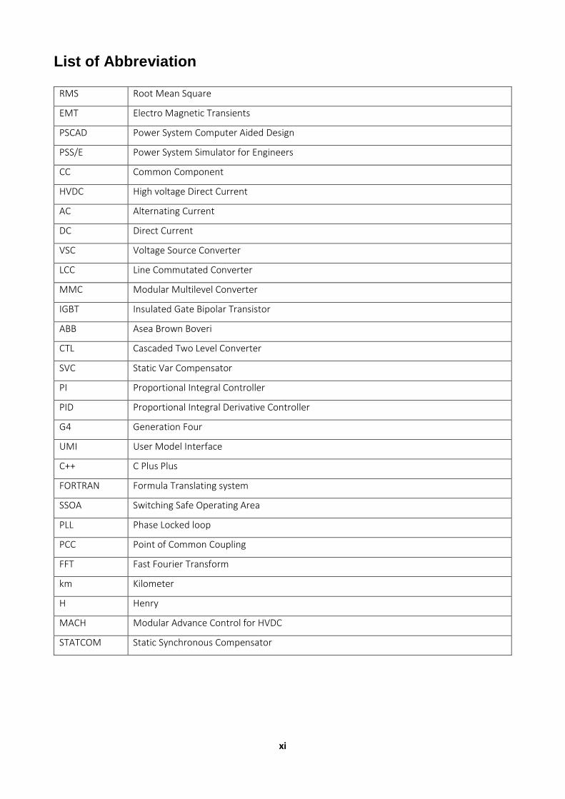
List of Abbreviation
RMS Root Mean Square
EMT Electro Magnetic Transients
PSCAD Power System Computer Aided Design
PSS/E Power System Simulator for Engineers
CC Common Component
HVDC High voltage Direct Current
AC Alternating Current
DC Direct Current
VSC Voltage Source Converter
LCC Line Commutated Converter
MMC Modular Multilevel Converter
IGBT Insulated Gate Bipolar Transistor
ABB Asea Brown Boveri
CTL Cascaded Two Level Converter
SVC Static Var Compensator
PI Proportional Integral Controller
PID Proportional Integral Derivative Controller
G4 Generation Four
UMI User Model Interface
C++ C Plus Plus
FORTRAN Formula Translating system
SSOA Switching Safe Operating Area
PLL Phase Locked loop
PCC Point of Common Coupling
FFT Fast Fourier Transform
km Kilometer
H Henry
MACH Modular Advance Control for HVDC
STATCOM Static Synchronous Compensator

xii
List of Tables
TABLE 1 ARGUMENT PASSING AND NAMING CONVENTIONS[11] ....................................................................................................... 16 TABLE 2: CALLING CONVENTION C++ [12] ................................................................................................................................... 16 TABLE 3 CALLING CONVENTIONS INTEL[13] .................................................................................................................................. 17

xiii

1
1 Introduction
1.1 Background
Demand in power across the globe with increased use of renewables, along with the growing power system, newer technologies and increased reliability are the motives in developing more efficient solutions in HVDC. Although AC is being commonly used for the past few years, the High Voltage Direct Current (HVDC) is equally an important part of this Power system.
HVDC helps in integrating the renewable sources of the energy from isolated parts of the globe to the mainland with lesser power loss and higher transmission efficiency. HVDC empowers AC systems of different frequencies to combine them to make a much smarter grid and thereby strengthen the grid.
In order to perform these errands suitably they are first simulated using simulation software appropriate for the study. The simulation helps to develop a simple and simplified model that can represent the actual power system. With new power plants and integration of them into the existing power system, there will be stability problems that can be studied with the simulation tools to ensure their safe implementation and operation.
1.2 Scope of Work
The objective of the thesis is to implement Common Component [4], the control system representation developed by ABB for RMS simulation tool to the EMT simulation tool, PSCAD. The Common Component is a simplified control system representation of the MACH control system used in EMT simulation. The CC represent the control signals for the converters used in the HVDC converter station.
EMT tools such as PSCAD/EMTDC are used to perform various studies such as Dynamic Performance studies (DPS), Sub Synchronous Transient Interaction (SSTI) studies, Etc. PSCAD represents the electrical system using differential equations, RMS and phasors while the mechanical parts of the system are signified using only differential equations.
RMS tools such as PSS/E, PowerFactory can perform planning and stability studies that can represent the electrical system by means of RMS or phasors while the mechanical system can be represented with differential equations. ABB widely uses both the tools for various studies.
The Common Component is implemented with PSSE, Power Factory and Netomac and being used as a common control system with the same code base in all the three tools for the simulation study. The Common Component is built using sequence components and phasors [4]. They are characterized by codes written in C++ and FORTRAN. The necessary changes made in Common Component during this thesis are in compliance with its interface to other tools.
The work is limited to model one converter station with fixed DC side voltage and operate in a specific control mode to ensure the system stability and control. The Common Component is currently developed for general representation of VSC HVDC light configuration and the simulations in PSCAD are carried out in the STATCOM Mode where only one station is simulated for the reactive power control/AC voltage control.
The document signifies the interfacing of the signals between both the components (Common Component and PSCAD) by implementing the RMS tool to the EMT tool. The PSCAD models are further built to obtain a stable system.
1.3 Outline
The thesis work constitutes the implementation of the control system and developing a model for the same in PSCAD. The work has been explained in detail with regards to the programming part of the interface and building the electrical model for the same.

2
Chapter 2 gives a theoretical background to the readers with regards to how HVDC was developed, its advantages over the AC, the different converter topologies, the converter topologies developed by ABB, the Common Component, which is the control system and an overview of the control system. This explains the control modes it is using and how they are designed for.
Chapter 3 gives an extract of how the Common Component is interfaced with the PSCAD. It is a programming concept that represents the control system by means of algebraic equations. Therefore some programming concepts have been explained that has aided the interfacing. It also explains how the PSCAD interface is done.
Chapter 4 explains the models that have been developed after the Common Component has been interfaced. There has been so far 4 models that has been employed testing the interface and that are still in development. With the tool that is being advanced, the model can be made more robust.
Chapter 5 discusses the various issues, results and things that can be improved with regards to the interfacing of the Common Component, the Common Component itself and the PSCAD models. This is followed by the conclusion and work that can be carried out in the future.

3

4
2 Theory
2.1 HVDC – An Overview
High Voltage Direct Current (HVDC), a technology developed by ABB about 50 years back is an emerging trend that has more advantage over the conventional AC system.
Alternating Current (AC) that is used everywhere around has its own shortcomings such as the transmission capacity handled by the AC cables, the losses associated with it and the distance limitation.
The advantages of HVDC are as follows:
An AC system requires three conductors while the HVDC requires only two conductors. This reduces the costs of line. [1]
The HVDC helps to interconnect asynchronous AC system of different frequencies that makes it possible to connect remote generation units and operates more effectively. [1] Additionally a thermal plant can be run more efficiently despite load variation on linking it to a hydro plant.
In AC, the reactive power flow causes large cable capacitance that limits the transmission distance while HVDC has the benefit that the cable can be designed for very long distances with no such drawbacks.[1]
HVDC has the advantage of controlling the active Power and hence becomes more flexible. The HVDC link can also impart control facilities on the AC and hence increase the performance of AC. There is better system stability achieved using HVDC. [1]
The overhead transmission line can be replaced by underground cables for DC transmission. This becomes more environmental friendly and there is much ease of operation. [1]
The HVDC losses are far more less when compared to AC for the same capacity, which includes the converter losses on HVDC side and consider cable losses between AC and DC cables.
Figure 1 Comparison of AC and DC Investment Costs [3]
HVDC requires more equipment’s such as the converters to convert from AC to DC and vice versa. This adds to the investment costs. But in reality, it must be noted that after a break even distance or critical distance(approx.. 600-800 km) [1] as shown in Figure 1, the total DC costs in less than total AC costs. Therefore it is necessary to choose between AC and HVDC system according to the individual case.
2.2 Principle of HVDC
HVDC is converting the generated AC to DC at a higher level and transmitting them over DC lines. They are then converted back into AC before being supplied to the distribution grid. Figure 2 shows the basic HVDC principle.

5
HVDC evolved in 1920’s where static converters and mercury-arc valves up to 1000 V was developed though they were not reliable and economic for high voltage. In mid-1940’s ABB made significant breakthrough that led to the first HVDC commissioning. The first HVDC transmission line, rated 20 MW, 200 A and 100 kV was installed in 1954 between the island of Gotland and The Swedish mainland that are 96 km apart and is functioning until this day.
The basic components of HVDC are discussed below
Harmonic Filters: Used to subdue the harmonics from the converters that can damage the capacitors and
Generators due to overheating and can also have interferences in telecommunication.
Converters: Made of valve bridges and transformers to operate in Rectifier mode (convert AC/DC) or in
Inverter Operation (convert DC/AC). The valve bridge is made up of high voltage valves of thyristors or IGBT
driven in a 6-pulse or 12-pulse mode.
Smoothing Reactors: Reactors with high value up to 1H is used in series with each pole to reduce harmonics
in the DC line, to prevent commutation failures and to avoid discontinuous current at low loads.
DC line: They can be overhead lines or underground lines of very long distance. The DC lines are similar to the
AC lines.
Shunt Capacitors: are also installed near the converters to compensate for the reactive power consumption by the converters. In steady state the converters consume about 50 % of the transferred active power and in transient state it is even higher.
Figure 2 HVDC Arrangement [3]
The DC links used in HVDC can be broadly designed into the following:
Monopolar Links It has one conductor and uses the ground or water as the return path. In cases where the earth sensitivity is high, a metallic return is used. This is very cost effective and used widely.
Figure 3 Monopolar Link [20]

6
Bipolar Links The converters at the terminals are usually rated same and has two lines as the name indicates. Hence the intersection of the converters are grounded. During fault, it is possible to still transmit half the load even if a pole is at fault.
Figure 4 Bipolar Link [20]
Homopolar Links As the name indicates the links are made up of two or more conductors having the same polarity. In DC transmission, the corona effect is lesser for negative polarity which is generally used for the homopolar links. The outlay is similar to the bipolar link except that the polarities for the links are the same.
Back-to-Back Links Two different systems (asynchronous systems having different voltage, phase or frequency) can be connected together by mean of Back-to-back links which houses the both converters under the same roof and the DC line length is kept as low as possible.
Multiterminal Links As the name indicates, this link has more than one point and it can be constructed according to all the above configurations. They can be connected in series and in parallel. Often parallel connection as seen in the Figure 7 are employed for large capacity station while series connection are used for low capacity connection. There can be hybrid connection which is a combination of both. The Multiterminal configuration is viable and commonly used since this technology allows power reversal by changing the direction of the current.
The configurations discussed above are in general terms and there are two significant configurations developed by ABB which are explained below.
2.3 HVDC Classic The HVDC Classic uses Line Commutated Converters to transfer power levels as high as 5000 MW that
has higher efficiency and dominates bulk power DC transmission. It has minimum short circuit ratio about twice of the converter rating. HVDC Classic is commonly used in very long subsea transmissions, long overhead line transmissions and high power transmissions. The HVDC converter station consists of valve building with the switchyard where the converters are current source converters.
Line commutated converters has switches that can be a valve or a switching element that connects each of the phase to one of the DC line as shown in Figure 8. These switches can only be turned on and there are two common configurations used based on the number of switches which are six pulse bridge and twelve pulse bridge. The losses are quite less in the converters, less than 1% per converter [15].
Figure 6 Back-to-Back Link [22]
Figure 7 Multiterminal Link [23]
Figure 8 Three phase Rectifier [24]
Figure 5 Homopolar Link [20]

7
The valves are capable of conducting current in one direction when a control or firing pulse is applied until the current is reduced to zero. Before the firing pulse is applied the valves are in non-conducting state capable of sustaining the voltage called as the forward blocking state. The valves conduct in pairs and the valves in one phase conducts until the valve in other phase is triggered to take over the current which is called commutation. In order to turn off the thyristors the converters must be connected to the AC system with synchronous machines to afford the necessary commutation voltage. Hence they are also referred to as Forced Commutated Converters.
Until the 1970’s Mercury arc valves have been used as valves while after that it is replaced by the thyristors until this day that can be controlled through a control pulse. In case of an uncontrolled operation, a diode is used as a valve. The shortcoming of LCC includes the valves conducting in one direction which gives almost constant DC current and hence power reversal is not possible. However the polarity of DC voltage can be changed at both stations to change the direction of power. The LCC depends on a very strong AC network to start up and uses often overhead lines that can help to interrupt in case of fault at DC side.
The HVDC classic converter consumes reactive power which initiates the necessity to use more filters or shunt banks to compensate for the balance of the reactive power in the system. Static Var Compensator (SVC) or synchronous compensators are used in few converter stations not only to balance the reactive power in the system but also to reduce the AC voltage step that is caused by the change in the active power.
2.4 HVDC Light
The HVDC light is capable of transferring power levels up to 1200 MW and is used widely in wind power integration, offshore power supply, underground transmission and connecting weak/asynchronous AC networks. There is no minimum short circuit capacity and is capable of black start in case of total blackout of the power system. The converter station houses all equipment’s except the transformers in a compact building which makes them compact and occupies less space. HVDC Light can be expanded to more terminals.
HVDC Light has more features in comparison with Classic. About 2000 km of HVDC light cables are in use and the Murray link (Australia) is the world´s longest land cable (180 km). The outstanding feature that makes it more compatible is that the DC cables for higher power transfer are actually lightly weighed extruded cable with prefabricated joint technology. They are quite economic and has no distance limitation or no induced circulating currents and no reactive power compensation is needed.
The Key feature of HVDC light is the heart of the converter station, the valves which consists of the IGBT’s that can be switched on and off as many times per cycle and improves the harmonic performance. Also there is no necessity to change the polarity of the converter station for power reversal and hence the converters have the DC voltage polarity fixed and there is a large capacitance at the DC side to smooth the DC voltage which makes the output more or less constant. This configuration is called Voltage Source Converter (VSC) or self-commutated converters.
‘The Voltage source converters using IGBT’s was introduced by ABB by means of HVDC Light. High voltages – in the hundreds of kV – are necessary for low-loss high-power transmission. This calls for series connection of a large number of insulated-gate bipolar transistors (IGBTs) when two level or three-level converters are used, which is challenging’.[7] A solution involving press-pack IGBTs with high-speed adaptive gate driving was developed in the mid-1990s; this solution has proven successful in service and under scaled laboratory conditions up to ±320 kV DC [8].
‘In subsequent stages of development, the switching frequency for two-level HVDC VSCs has been brought down from 2 kHz to about 1 kHz in order to reduce losses [7]. It may be possible to go even further, but this would call for increased filtering, which would partly outweigh the benefits. [7] One further limitation of VSC technology is the current capability of the IGBT. Today, the largest available IGBT has a maximum turn-off current of 4000 A, effectively giving 1800 A dc transmission. [7] Multilevel VSC technology without IGBT

8
series connection has been introduced on the market. Although promising in many respects, extra equipment is required in order to safely handle different fault scenarios’. [7]
The self-commutated converters can feed power to AC network entailing passive loads. Also VSC does not absorb reactive power, there is no necessity of compensations and hence there is independent control of real and reactive power flow. The power reversal in this case takes place by changing the current direction.
Figure 9 Voltage Source Converter [25]
The real and reactive power control takes place irrespective to the converter station and in the rare case ever if a trip occurs in one of the HVDC light converter, the other converter will continue to operate in AC voltage/reactive control mode that is the Statcom mode. There is also lower possibility of commutation failure as only switching takes place at the DC terminals.
2.5 Converter Topology and Main Circuit
A cascaded two level converter (CTL) has series-connected press-pack IGBTs used in the valves that can be cascaded for high voltage two-level VSCs to multilevel VSCs. [7] The CTL consists of two arms, a positive and negative which forms respectively the positive and negative terminals of the DC side. As seen in Figure 10 each arm has a cascade of two level IGBT’s. The cascaded two-level cells in each arm are controlled to provide fundamental-frequency output voltage, related to the desired active and reactive power output, through switching of the individual cells, as will be described momentarily.[7]
Figure 10: Single line diagram of CTL [7]
For a two level converter made up of two transistors T1 and T2 with diodes in parallel to them D1 and D2 there are three ways in which they can be operated in:

9
When T2 is on and T1 is off, the output voltage charges to equal the voltage across the capacitor. The capacitor is charged on positive current in the arm and discharges when negative current. [7]
When T1 is turned on and T2 is turned off, the output voltage is constant and the capacitor is bypassed. [7]
When T1 and T2 are turned off, the diodes conduct current but only in one direction. When the arm current is positive the capacitor gets charged. [7]
The cells are cascaded to give higher voltages that forms the modular multilevel converter (MMC). The major disadvantage of VSC is that there is about 1.1 % losses per converter. [7]
2.6 Common Component
According to the developers of Common Component “Instead of writing the model for HVDC Light in different simulation tools as user defined component, a ‘Common Component’ is developed which represents the detailed control functionality of HVDC Light.”[4]
The Common Component is a general representation of the control system designed especially for the HVDC light and can be linked to different simulation tools using appropriate user model interfaces. [4] This tool independent modelling approach is particularly useful for upgrade and maintenance of models with utmost quality especially when the product is under constant development.”[4]
The concept of Common Component can be explained as a tool developed to represent the control system of a power system products described by a system of differential-algebraic equations (DAE). [4] It performs computations related to initialization, time derivatives and numerical integration [4] and various other algebraic functions.
The arguments of CC subroutine are comprised of the following four types of quantities:
Model constants, state and internal variables
Main circuit parameters and measurements
Simulation control signals.
Output quantities of the HVDC Light controller.
The advantages of the above strategy are as follows:
The major advantage of Common Component is that the same control tool can be used with other simulation tool for various studies without losing its compliance. [4]
Using the Common Component with other simulation tools requires an interface specific to the tool used. There will not be much change with the control part of the component. [4]
Products such as HVDC Light is continuously developed and hopefully with a Common Component the model of such products implemented in different tools can be updated at the same time.
Figure 11 CC based model development strategy for HVDC Light [4]
HVDC Light

10
Figure 11 represents model development strategy, the Common Component which is the control system of HVDC Light communicates with the AC and DC system through appropriate tool dependent user model interfaces (UMI). It should also be noted that the AC and DC systems are designed and modelled specific to the tools used and hence the interface of the Common Component needs to be designed specific to the tool used. The Common Component gives the necessary pulses to the converter to control the necessary voltage/power/frequency.
The basic control for the converter are Active Power/Dc voltage control and Reactive power/AC voltage control. The control system has four control modes which can be set initially. On setting it to Active Power control, Pref is set up as the reference for the converter control. Similarly the other reference values and control can be set up to achieve the proper control. Also it helps to safeguard against DC overvoltage’s and AC overcurrent stress when subjected to faults or disturbances.
The control is designed on two basic control modes, Active Power/Dc voltage control and Reactive power/AC voltage control by having a reference value and to make sure it is well maintained at a margin close to the reference for about ±1%. There are also controls based on self-protection of the system during faults and its recovery after faults within the time limits.
Switching Safe Operating Area (SSOA) enables the converter to obstruct the cells when the converter current or cell voltages are out of the SSOA. If the peak values crosses the border for current and voltage, then there is an instant trip. The Switching Safe operating Area of a transistor is shown in Figure 12.
Figure 12 SSOA [26]

11
2.7 Schematic Overview of the Control system
Figure 13 Schematic of Control system [17]
The DC voltage control/Active power control in one station will affect other stations in a DC system while for the AC voltage control/Reactive power control in one station will not affect other stations in a DC system. The current reference for the control system can be measured from the Pref and Qref that enables to calculate the voltage out from the converter Uv (amplitude, frequency and phase) to fulfill that reference.
Figure 14 dq Reference [6]
The measured quantities in the AC system are three phase that are not suitable while designing the control system as they are oscillating with system frequency in steady state. Hence it is more prudent to have quantities in steady state that enables the use of PI controllers. This can be achieved by transferring the three phase quantities into two phase quantities which can be controlled utilizing standard controllers such as PI controllers.
2.7.1 abc to αβ Transformation
The figure shows the transformation between the two coordinate axes namely the abc and αβ coordinate systems. The a-axis is aligned as same as α-axis.
The Clarke or αβ transform is a space vector transformation of time-domain signals (e.g. voltage, current, flux, etc) from a natural three-phase coordinate system (ABC) into a stationary two-phase reference frame αβ[6].
[
𝑢𝛼(𝑡)𝑢𝛽(𝑡)
𝑢0(𝑡)] =
2
3
[ 1 −
1
2−
1
2
0√3
2−
√3
21
2
1
2
1
2 ]
[
𝑢𝑎(𝑡)
𝑢𝑏(𝑡)𝑢𝑐(𝑡)
] (2.7.1)
If the voltage u is positive sequence
[
𝑢𝛼(𝑡)
𝑢𝛽(𝑡)
𝑢0(𝑡)
] = (
�̂� 𝑐𝑜𝑠𝜃(𝑡)
�̂� 𝑐𝑜𝑠𝜃(𝑡 −2
3𝜋)
�̂� 𝑐𝑜𝑠𝜃(𝑡 +2
3𝜋)
) (2.7.2)
Figure 15 Phasor reference [6]

12
And on transformation it comes to
[
𝑢𝛼(𝑡)𝑢𝛽(𝑡)
𝑢0(𝑡)] = (
�̂� 𝑐𝑜𝑠𝜃(𝑡)�̂� 𝑠𝑖𝑛𝜃(𝑡)
0
) (2.7.3)
u is transformed to a rotating phasor in a fixed coordinate system uαβ = uα + juβ = �̂�𝑒𝑗𝜃(𝑡)
2.7.2 αβ to dq Transformation
In order to obtain dc quantities that can be used for vector current control the rotation must be removed. This
enables to design the conventional PI controller. The rotation of the vector (dq-transformation) can be done
according to:
Figure 16 Phasor Reference [6]
U = 𝑢𝑑 + 𝑗𝑢𝑞 = 𝑒−𝑗𝜃(𝑡)𝒖𝛼𝛽 (2.7.4)
Or
[𝑢𝑑
𝑢𝑞] = [
𝑐𝑜𝑠𝜃 𝑠𝑖𝑛𝜃−𝑠𝑖𝑛𝜃 𝑐𝑜𝑠𝜃
] [𝑢𝛼
𝑢𝛽] (2.7.5)
The dq-frame rotates in the -frame with the
fundamental frequency. The positive sequence becomes a
dc component and a negative sequence becomes an AC
component which rotates clockwise with twice the
fundamental frequency.
When dq is aligned to the converter bus voltage, the current in the d-direction is active current while
the current in the q-direction is reactive current. The calculation of θ is vital since it aligns the rotating frame
along the stationary frame. Or in other words the dq is aligned to the converter bus voltage which is achieved
by using a PLL-Phase Locked Loop.
The system angle is computed via the principle that the PI controller uses the positive sequence part
of the q-component of the voltage as control error. This means that the system angle is computed in order to
obtain zero 𝑢𝑐𝑜𝑛𝑣,𝑞 in steady state, thus the full voltage is projected on the d-axis.
2.7.3 Converter Outer Loop
The instantaneous power can be calculated as the sum of
each phases active powers in case of a three phase system which is
given by the equation
𝑆 = 𝑢𝑎𝑖𝑎 + 𝑢𝑏𝑖𝑏 + 𝑢𝑐𝑖𝑐 Applying the transformation from ABC to αβ to dq.
(2.7.6)
Figure 17: 𝑢𝑐𝑜𝑛𝑣,𝑞 ≠ 0 [6]
Figure 18: 𝑢𝑐𝑜𝑛𝑣,𝑞 = 0 [6]

13
𝑃 = 3
2𝑅𝑒{𝒖𝛼𝛽(𝒊𝛼𝛽)
∗} =
3
2𝑅𝑒{𝒖𝑑𝑞(𝒊𝑑𝑞)
∗}
𝑃 = 3
2(𝑢𝛼𝑖𝛼 + 𝑢𝛽𝑖𝛽) =
3
2(𝑢𝑑𝑖𝑑 + 𝑢𝑞𝑖𝑞)
From the graph, in steady state on aligning the voltage to the d-axis 𝑢𝑞 = 0 that implies that the d part of the phase current will control
the active power
𝑃 = 3
2𝑢𝑑𝑖𝑑 (2.7.7)
Figure 19 Phasor Reference [6]
Similarly the reactive power can be written as
𝑄 = 3
2𝐼𝑚{𝒖𝛼𝛽(𝒊𝛼𝛽)
∗} =
3
2𝐼𝑚{𝒖𝑑𝑞(𝒊𝑑𝑞)
∗}
𝑄 = 3
2(𝑢𝛽𝑖𝛼 − 𝑢𝛼𝑖𝛽) =
3
2(𝑢𝑞𝑖𝑑 − 𝑢𝑑𝑖𝑞)
In steady state,𝑢𝑞 = 0, Hence, 𝑄 = −3
2𝑢𝑑𝑖𝑞 (2.7.8)
Thereby by controlling the d-component, the active power/DC voltage control is realized and on normalizing
the q-component, the reactive power/AC voltage control can be made.
2.7.4 DC Voltage Control / Active Power control
The control principle is that the current order will be increased if the reference voltage is higher than
the measured value, which also implies that a positive current order will lead to active power transferred
from AC to DC side (rectifier) and vice versa. The direction of the power flow can be changed by reversing
the DC voltage. The DC current does not change the direction.
Figure 20 DC Voltage/Active power control [16]
The control system shown in Figure 20 represents the DC voltage control/ active power control mode.
The control fires the IGBT’s according to the pulses of the AC system. The PI controllers enable the control of
the firing angles. The Idc and Udc control consisting of values compared against the reference value and the

14
output of which triggers the PI controllers to control the converters. The extinction angle control is used to
maintain stability margins. There is an allowed minimum value, below which the extinction angle control will
be activated.
2.7.5 AC Voltage Control / Reactive Power Control
The AC voltage controls the voltage at primary side PCC (AC network side) of converter transformer
to the reference setting. The Ac voltage and current are used to calculate the reactive power within the system.
This measured value is compared with the reference value and if they are within the allowable range. Based
on if the reactive power is higher or lower than the reference value, the current is controlled to give the desired
reactive power control. Thus a simple PI controller is used for the same.
2.7.6 Positive and Negative Sequence Components
AC networks are seldom perfectly symmetrical, which implies that the voltage/current of the AC network often contains both the positive and negative sequence components. From control point of view, it is desired to separate the positive and negative sequence components. Otherwise, the oscillation with twice the fundamental frequency may disturb the key functional blocks, such as the PLL and the current control, AC voltage control. Furthermore, the negative sequence component can be also directly used to evaluate the size of asymmetrical AC fault. Positive and negative sequence sets contain those parts of the three-phase excitation that represent balanced normal and reverse phase sequence. [18] Zero sequence is required to make up the difference between the total phase variables and the two rotating components. [18]
2.8 Per-Unit System
The power system typically comprises of various voltages and power due to the presence of
transformers and hence calculating the voltage and current at different levels are quite complex. To simplify
the system calculations, the electrical system quantities are normalized by selecting some base values. This is
called the Per Unit or pu system.
Per unit of different system quantities is represented by the following equation [2]
𝑄𝑢𝑎𝑛𝑡𝑖𝑡𝑦 (𝑝𝑒𝑟 𝑢𝑛𝑖𝑡) = 𝑄𝑢𝑎𝑛𝑡𝑖𝑡𝑦 (𝑛𝑜𝑟𝑚𝑎𝑙 𝑢𝑛𝑖𝑡𝑠)
𝐵𝑎𝑠𝑒 𝑉𝑎𝑙𝑢𝑒 𝑜𝑓 𝑞𝑢𝑎𝑛𝑡𝑖𝑡𝑦 (𝑛𝑜𝑟𝑚𝑎𝑙 𝑢𝑛𝑖𝑡𝑠) (2.8.1)
Usually the base values are chosen from the apparent power (𝑆𝑏𝑎𝑠𝑒) which is constant throughout
the system and the line to line voltage (𝑉𝑏𝑎𝑠𝑒) that changes with the turns of the transformer ratio.
The per unit values of different system quantities are shown below [2]:
𝑉𝑝𝑢 = 𝑉𝑎𝑐𝑡𝑢𝑎𝑙
𝑉𝑏𝑎𝑠𝑒 (2.8.2)
𝑆𝑝𝑢 = 𝑆𝑎𝑐𝑡𝑢𝑎𝑙
𝑆𝑏𝑎𝑠𝑒 (2.8.3)
𝐼𝑝𝑢 = 𝐼𝑎𝑐𝑡𝑢𝑎𝑙
𝐼𝑏𝑎𝑠𝑒 , 𝐼𝑏𝑎𝑠𝑒 =
𝑆𝑏𝑎𝑠𝑒
𝑉𝑏𝑎𝑠𝑒 (2.8.4)
𝑍𝑝𝑢 = 𝑍𝑎𝑐𝑡𝑢𝑎𝑙
𝑍𝑏𝑎𝑠𝑒 , 𝑍𝑏𝑎𝑠𝑒 =
𝑉𝑏𝑎𝑠𝑒2
𝑆𝑏𝑎𝑠𝑒 (2.8.5)
During this transformation, the entire system can be simplified by representing it as impedances
thereby eliminating different voltage and power levels that makes the system calculation more complicated.
This method is more feasible for computer simulation of system study.

15
3 Implementation of the CC in PSCAD
3.1 Control Implementation
ABB Power Systems uses HiDraw, a fully graphical block programming language [9], and HiBug, a fully
graphical debugger, both operating under Windows on networked industry standard PCs. [9] Hidraw is vey
user friendly as it is built with various blocks that can be dragged and dropped and connected. Hidraw is
capable of generating codes with the building blocks used in high level languages such as C, FORTRAN, PL/M
or in assembly language (low level languages). [9]
The control system referred here as the Common Component have been developed by ABB in Hidraw pages where individual controls are represented at unique pages and each pages consists of inbuilt blocks that can define the specific control. All functions of Common Component are represented graphically in different pages. The signals can be transferred between the different pages containing the functions. From this page, the C++ code is generated.
Figure 21 Hidraw
As the Hidraw cannot be supplied to the customers in order to make use of the Common Component, there is a special feature where the Hidraw pages can be converted to some programming codes. Thereby the Common Component are now available in C++ and FORTRAN codes. So basically it is some programming codes compiled together to be interfaced to the respective tool it is to be interfaced with. So far the common codes been interfaced with Digsilents Powerfactory, PSS/E and Netomac tools. It is very common now for the utilities to use PSCAD and hence interfacing CC into the PSCAD would be worthwhile.
Figure 22 PQMVA calculation in Hidraw

16
3.2 Interface Implementation
PSCAD has an internal library consisting of the inbuilt components and the basic language used to write the instruction or codes is FORTRAN. The system is built in PSCAD that measures and sends the necessary value to the control system. Therefore an interface is required to communicate between PSCAD and the Common Component. A C++ interface has been developed so as to pass the values between the PSCAD and Common Component. But since PSCAD uses FORTRAN while the interface is in C++ compiler flags are needed for the compiler to recognize the nature of the parameters if it is a character, float or an Integer which is passed between the C++ and the FORTRAN segment in PSCAD. Common Component consists of header files, C++ files and a FORTRAN
file that represents each function of the control system. These files are compiled into a library which can be linked into the PSCAD simulation so that it can recognize where the Common Component is and all the files with regards to this. This is made possible by creating a batch file. A batch file [10] is used to perform a repetitive tasks or routine using conditional branching and looping certain.
The compiler flags are set in the batch file specific to the FORTRAN and the C++. The compiler flags contains the calling conventions that allows one to specify conventions for passing arguments and return values between functions and callers. [11]
Keyword Stack Cleanup Parameter Passing
Cdecl Caller Pushes parameters on the stack in reverse order (right to left)
Clrcall n/a Load Parameters onto CLR expression stack in order (left to right)
Stdcall Callee Pushes parameters on the stack, in reverse order (right to left)
Fastcall Callee Stored in Register, then pushed in stack
Thiscall Callee Pushed in stack; this pointer stored in ECX
vectorcall Callee Stored in Registers, then pushed on stack in reverse order (right to left) Table 1 Argument Passing and Naming conventions[11]
These options determine the order in which function arguments are pushed onto the stack, whether the caller function or called function removes the arguments from the stack at the end of the call, and the name-decorating convention that the compiler uses to identify individual functions. [12] A few examples for calling conventions for visual C++ are listed below:
/Gd _cdecl calling convention
/Gr _fastcall calling convention
/Gz _stdcall calling convention
/Gv _vectorcall calling convention Table 2: Calling Convention C++ [12]
The FORTRAN on the other hand has the following calling conventions. The FORTRAN compiler used here is Intel.
/iface:default Tells the compiler to use the default calling conventions. These conventions are as follows: The calling mechanism: C
The argument passing mechanism: by reference
Character-length argument passing: at end of argument list
The external name case: uppercase The name decoration: Underscore prefix on IA-32 architecture, no prefix
on Intel® 64 architecture; no suffix
PSCAD (FORTRAN)
C++ Interface
CC (C++)CC(Fortran)
CC (C++)
C++ Interface
Figure 23 Interface

17
/iface:cref Tells the compiler to use the same conventions as /iface:default except that external names are lowercase.
/iface:cvf The calling mechanism: STDCALL on Windows* systems using IA-32 architecture
The argument passing mechanism: by reference
Character-length argument passing: following the argument address
The external name case: uppercase
The name decoration: Underscore prefix on IA-32 architecture, no prefix on Intel® 64 architecture. On Windows* systems using IA-32 architecture, @n suffix where n is the number of bytes to be removed from the stack on exit from the procedure. No suffix on other systems.
/iface:mixed_str_len_arg Specifies argument-passing conventions for hidden-length character arguments. This option tells the compiler that the hidden length passed for a character argument is to be placed immediately after its corresponding character argument in the argument list. This is the method used by Compaq Visual Fortran*. When porting mixed-language programs that pass character arguments, either this option must be specified correctly or the order of hidden length arguments must be changed in the source code. This option can be used in addition to other /iface options.
/iface:stdcall The calling mechanism: STDCALL
The argument passing mechanism: by value
Character-length argument passing: at the end of the argument list
The external name case: uppercase
The name decoration: Underscore prefix on IA-32 architecture, no prefix on Intel® 64 architecture. On Windows* systems using IA-32 architecture, @n suffix where n is the number of bytes to be removed from the stack on exit from the procedure. No suffix on other systems.
/iface:stdref Tells the compiler to use the same conventions as /iface:stdcall except that argument passing is by reference.
Table 3 Calling conventions Intel[13]
As can be seen from Table 2 and Table 3 proper calling conventions need to be chosen for the parameters to be passed between C++ and Fortran. Unlike other tools like PSS/E and powerfactory, PSCAD required iface:default and iface:mixed_str_len_arg, as a part of Intel Compiler flags and /Gm, /Gd, /ZI, for C++ compilation, upon which the Common Component was interfaced successfully with PSCAD. It is possible to pass the values that includes float, integer and characters between PSCAD and Common Component.
Code 1 shows the struct that is being passed onto the Common Component and Code 2 shows the
interface that accepts the struct from the PSCAD. Code 3 illustrates the values being passed to the Common Component and calling the main function that starts the control system that is displayed in Code 4.
The Common Component is developed to be started from the load flow/initialization. PSS/E and
Powerfactory has inbuilt load flow options that enables for proper load flow calculations and thereafter stabilizing the system. PSCAD on the other hand does not have load flow solution and it has to be started from zero and wait for the system to stabilize.
Another important part of the Common Component are the feedback signals that are to be used for the next time step. The memory allocation for these signals are very important as the right signals needs to be passed and the values are to be compared with the previous time step for the right output. The interface however is not able to accept the Integers but on converting them to float values, it was able to pass the integer values. This is due to the compiler options between the interfaces that needs further investigation.

18
3.3 Electrical Implementation
After the interface the system is designed for STATCOM mode of operation with one converter station and the other end of the DC side is supplied with a constant DC voltage as shown in Figure 27.
The AC system consists of a 3-phase system connected to the converters (represented by a three
phase source here). This is shown in Figure 24. There are three 3-phase system consisting of a strong network, a weak network or when in case of an extremely weak network which is helpful in case of simulating a complete blackout or fault case. A strong network is being used in this simulation.
Figure 24 AC System
Figure 27 depicts how the HVDC system is represented. The bus is connected with the three phase AC system and is stepped up using a three phase transformer. The multimeters are used to measure the current and voltage which are fed to the control system. The current and voltage are measured at two points, at PCC (point of common coupling) and the converter bus. The converter are represented by a three phase source which has the output from the control system. The DC side can be seen to be represented by two DC sources connected in series to each other and maintain the DC side voltage to be 300 kV.
Figure 25 Statcom Mode
Figure 26 Tap Changer Setting
Figure 27 HVDC System

19
Figure 28 is a component that gets all the inputs from the electrical system and calls the Common
Component. The REF_CC is a vector of six elements where the reference values of Real power, reactive power, Ac voltage, Dc voltage are sent in. The CTRL_CC is a vector of 7 elements where the control signals are set in for the control system to recognize if the system is in AC voltage/ Reactive power mode or in DC voltage or in Real power mode. The current and voltages are rms measurements from the multimeter that are converted to alpha and beta components and it is important to note that these values are in per-unit.
Iv_Alpha and Iv_Beta represents the converter side current in Alpha and Beta while U_Conv_A and
UConv_B is the converter side voltage in Alpha and beta. Similarly, I_PCC_A and I_PCC_B are the PCC current while U_PCC_A and U_PCC_B are PCC side voltages. Udc_PU is the per-unit measurement of voltage at the DC side. P_nom is the nominal DC side power. TrRatio is the transformer tap changer which is calculated as shown in Figure 26. TRF and IRF are the outputs from the Common Component that are plotted in graphs shown in Figure 29.
Figure 28 Control system
The output from the control is converted to actual value and to three phase voltage which is fed back
to the system via a three phase voltage source. The outputs are converted from rectangular to polar where the magnitude is the three phase voltage while the phase is the phase difference. The standard parameters for the control are also shown where the Base AC voltage, frequency and DC voltages are shown.
Within this control system the script to pass the values to the Common Component are written using
a struct. This is shown in Code 1. This explains the basic way of modelling the system. The parameters used in the system are from a typical VSC system parameters for 132 kV/400 kV configuration and the values used in the model for designing the system are from the Powerfactory model that interfaced the Common Component. The parameters are referenced in Appendix B.

20
Figure 29 Output TFR and ITR

21
4 Models and Simulation Results The PSCAD model is set in statcom mode in reactive power control mode where 𝑄𝑟𝑒𝑓 = 200 MVar.
There are four different models that are being worked upon. The models have different inputs such as instantaneous measurement values, RMS measurement values and constant input values. The Output is analyzed to get the referred reactive power and verify that the system is stable.
The challenge in using PSCAD is that it is an EMT tool that works with instantaneous values and the Common Component is an RMS tool that requires the input as RMS values. It is possible to measure the RMS voltage in PSCAD and with PSCAD Version 4.6.0 it is possible to measure the RMS current. But the measured RMS value which is of one dimension cannot be converted to dq or 𝛼𝛽 in PSCAD. Hence, there are two models that are being considered to design the electrical representation of the converter side of the system.
4.1 Model 1
As explained above the model is set in Statcom mode. The reference 𝑄𝑟𝑒𝑓 = 200 MVar is set in the
Reference vector. The instantaneous voltages and currents measured consists of three quantities (A, B, C)
representing each phase. The three quantities are converted to two quantities using ABC to 𝛼𝛽 conversion.
But it is to be observed that 𝛼𝛽 is a time varying quantity while the Common Component expects the quantity
in rms that are not time varying. Therefore the 𝛼𝛽 quantities are thereafter converted to a dq. Figure 30
depicts the same. The voltages and currents at the PCC and converter buses are converted to per unit values
based on their respective per phase Base values before being fed to the control system.
Figure 30 Model 4.1.1
In Figure 31 the voltage per unit output (dq) from the control system are converted back to three phase
actual values through 𝛼𝛽 quantities with respective to the same base values as the input. The obtained three
phase are then fed through three independent DC sources that would not modulate the obtained signals from
the control system. The system simulation results can be compared with that of the simulation results from
PowerFactory Figure 33. The simulation in PSCAD is executed for 2.5 s and the results are shown in Figure 32.
The real power is seen to be close to zero while the reactive power is seen to be close to 200 MVar.
The voltages in the system are quite low. At the PCC bus to be about 127 kV instead of 132 kV while at
the converter bus it is 173 kV rather than 195 kV. As mentioned earlier, the Common Component calculated
the power (real and reactive) and compares them with the reference value that are then given to the
controllers to influence the voltage accordingly. This might be because of the losses within the system though

22
this is not acceptable. Therefore the inputs of the control system (Figure 34) are compared against the inputs
used in the PowerFactory Implementation.
Figure 31 Model 4.1.2
It can be seen from Figure 33 and Figure 34 that the inputs are opposite to the ones in PF. For example,
the alpha quantity of voltage at the PCC bus is close to 1 for PF, but it is close to zero for PSCAD. While the
beta quantity of voltage at PCC buss is close to zero in PF but it is negative and close to one for PSCAD.
Therefore different models are being investigated to get the desired results. The Common Component is
debugged internally to check for errors since there is no initialization taking place at the PSCAD and the results
are to be compared at steady state. It has been found that, there are some divide by zero error caused by no
initialization and those places have been replaced by some minimum values or zero.
Figure 32 P,Q Measurement
This is a very simple and robust model that can be used under normal condition. But as it can be seen
the inputs to the Common Component are not being properly obtained. Another reason can be that the
Common Component does not start from load flow as seen in Figure 34 in PSCAD, there is a problem building
up to the steady state with the Common Component that still needs to be investigated.

23
Figure 33 PF Voltage and Current Inputs
Figure 34 Results V,I
24
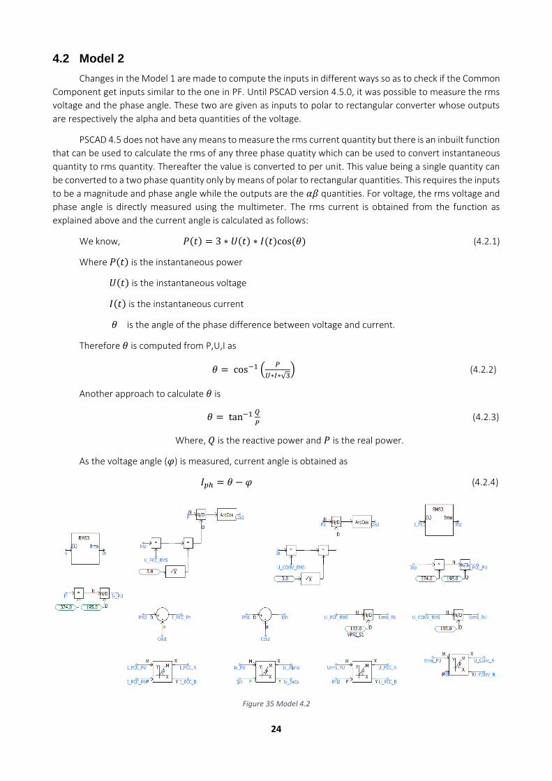
4.2 Model 2
Changes in the Model 1 are made to compute the inputs in different ways so as to check if the Common
Component get inputs similar to the one in PF. Until PSCAD version 4.5.0, it was possible to measure the rms
voltage and the phase angle. These two are given as inputs to polar to rectangular converter whose outputs
are respectively the alpha and beta quantities of the voltage.
PSCAD 4.5 does not have any means to measure the rms current quantity but there is an inbuilt function
that can be used to calculate the rms of any three phase quatity which can be used to convert instantaneous
quantity to rms quantity. Thereafter the value is converted to per unit. This value being a single quantity can
be converted to a two phase quantity only by means of polar to rectangular quantities. This requires the inputs
to be a magnitude and phase angle while the outputs are the 𝛼𝛽 quantities. For voltage, the rms voltage and
phase angle is directly measured using the multimeter. The rms current is obtained from the function as
explained above and the current angle is calculated as follows:
We know, 𝑃(𝑡) = 3 ∗ 𝑈(𝑡) ∗ 𝐼(𝑡)cos (𝜃) (4.2.1)
Where 𝑃(𝑡) is the instantaneous power
𝑈(𝑡) is the instantaneous voltage
𝐼(𝑡) is the instantaneous current
𝜃 is the angle of the phase difference between voltage and current.
Therefore 𝜃 is computed from P,U,I as
𝜃 = cos−1 (𝑃
𝑈∗𝐼∗√3) (4.2.2)
Another approach to calculate 𝜃 is
𝜃 = tan−1 𝑄
𝑃 (4.2.3)
Where, 𝑄 is the reactive power and 𝑃 is the real power.
As the voltage angle (𝜑) is measured, current angle is obtained as
𝐼𝑝ℎ = 𝜃 − 𝜑 (4.2.4)
Figure 35 Model 4.2

25
Figure 35 shows that the instantaneous currents are converted to rms values while the phase angles
of the currents are calculated from the voltage angle and the phase shift angle as in Equation 4.2.3 and 4.2.4
The voltage and current RMS magnitude and phase angles are then given as inputs to the polar to rectangular
converter that gives the 𝛼𝛽 quantities which are fed to the Common Component. The Common Component
has a PLL within the code that will assist in calculating 𝜃 (necessary to estimate the inclination between the
rotating and synchronous reference frame for 𝛼𝛽 − 𝑑𝑞 transformation) and converting 𝛼𝛽 quantities to dq
transform.
Iv is the measured converter current while I_PCC is the measured current at PCC bus. The two currents
are instantaneous values and are converted to RMS using a PSCAD built in function. The RMS values are then
converted to p.u. by dividing them by its base. The current angle at the PCC and converter bus on the other
hand is computed at every time step using equation 4.2.2 and 4.2.4. The angles are in radians. The RMS voltage
at the converter (U_CONV_RMS) and PCC (U_PCC_RMS) bus are measured using multimeter connected in the
system. They are then converted into the PU values. The voltage angles are also measured using the voltmeter.
The magnitude and the angle are then converted into rectangular form using polar to rectangular
transformation. The rectangular co-ordinates represent the alpha and beta of the corresponding quantities.
The output from the Common Component are converted from rectangular to polar quantities and to actual
values and are fed back to the system using a three phase voltage source as shown in Figure 36.
The simulation is executed with the same parameters as Model 1 for a simulation time of 2.5s in Reactive
power control mode. But it can be seen from Figure 37 that the reactive power is far away from the reference
value and there is no actual reactive power control taking place. The real power is close to zero according to
the reference value while the reactive power is less as about 40 MVar when it needs to be 200 MVar according
to the reference value. Therefore the inputs to the Common Component are analyzed once again. This model
does not give better results compared to Model 4.1.
Figure 36 System design of Model_4.2

26
Figure 37 P,Q-Model_4.2
On comparing the voltages and currents between the PF and PSCAD model, it is quite close to that of
the PF as per in Figure 33 and Figure 38. Initially there are transients that occurs because of the initialization
taking place within the Common Component but then at the steady state it has settled to a value close to the
one in PF. On debugging the signals internally in the control system, it was discovered that there occurs
instances of infinity that has been replaced by 0. There was two instances where it occurred initially because
of the divide by zero error but has been replaced by a condition if the denominator is zero then the output
value is zero.
These changes in the Common Component needs to be done such that they will not affect the other
tools that it has been implemented in already. It can be seen that modelling the system by calculating the rms
current and its angles gives better results than that of the conversion method. The decrease in the reactive
power is because of some change in the control system or due to wrong measured value that is to be
debugged.

27
Figure 38 V.I comparison of PF and PSCAD Model 4.2
Figure 39 Model 4.3
4.3 Model 3
To investigate if there is a problem with how the circuit is modelled or if the control system is not
compatible for PSCAD since the significant change is running the control without initialization. Hence the
control system is checked by giving the inputs from the PowerFactory to the control system in the
Powerfactory and looking up the results of the real and reactive power. Figure 39 shows constant input given
to the system.
Figure 40 shows the real and reactive power obtained from the model. The real power is close to zero
while the reactive power is quite less about 160 MVar and the voltage is high at the PCC bus, about 140 kV
while the input is only 132 kV. This is quite high and can cause overheating and further breakdowns and faults.
Therefore it is important to modify the control system so as to start from initialization that will become
compatible with the tool, PSCAD.
Figure 40 P,Q of Model 4.3

28
4.4 Model 4
Model 4 is developed in PSCAD version 4.6.0 where it is able to measure the rms current using the
multimeter and the angles are measured by the FFT blocks.
Figure 41 PSCAD 4.6.0 Model
A different approach to implement the same idea as that in Model 4.2. The voltage and current
magnitudes are measured using the multimeter and they are converted to PU values. The angles of the same
are computed using the FFT blocks as seen in Figure 41. According to PSCAD, Fast Fourier Transform (FFT) can
determine the harmonic magnitude and phase of the input signal as a function of time. The input signals first
sampled before they are decomposed into harmonic constituents. [14]
The feedback from the control system and the system design are the same. The internal signals have
been debugged for eliminating the divide by zero error. Hence the system does not break in between. But the
results are quite unexpected. The P, Q control is nowhere attainable from Figure 42. The real power that needs
to be zero for Reactive Power Control is actually about 170 MW while the reactive power that has a reference
value of 200 MVar is about 1100 MVar which is highly not acceptable and this method does not prove to be
so worthy.
It is also noted that some changes are made within the Common Component that also contribute to
disruption here as this change here is quite obscured. The FFT could also cause such a huge difference as the
phase angles plays an important role in computing the rectangular coordinates. Due to the discrete nature of
the algorithm, any sub-harmonics or inter-harmonics present in the measured signal will interfere with the
output. The measured signal should be free from inter-harmonics and sub-harmonics for accurate results. [14]

29
On observing the Figure 43, the voltage and current alpha and beta inputs measured at the PCC and
converter bus are quite uncertain as well. This will lead to the possibility that power will be high when
calculated but still the fact stays that there is a limiter that needs to control the system in such case. Hence
the electrical representation needs to be further investigated with regards to the real and reactive power
which in turn is due to the input parameters.
Figure 43 V,I of Model 4
Figure 42 P, Q of Model 4

30
5 Discussion
5.1 Common Component Interface
Developing the interface for PSCAD was quite a challenge because of the new kind of interface it is going
through. There has been interfaces between PSCAD and C++ implemented and corresponding examples are
available. The major difference here is that there is another interface from the C++ to the FORTRAN and that
needs to be taken into consideration.
On looking at the batch file developed for PSS/E which is also having the same interface, /Gz is used as
C++ compiler option while /iface:cvf is used as FORTRAN option.(Table 2 and Table 3) The same option is not
valid when used in PSCAD. There is a linking error, NMAKE that comes up in this case. For the communication
between PSCAD and the interface the following compiler flags /Gm, /Gd, /ZI are chosen for C++ and /iface:
default and /iface: mixed_str_len_arg are choosen for the FORTRAN compiler.
There are three types of variables that are needed to be passed to the Common Component. The
integers, float and character values. So far the float and characters are being able to be passed between the
PSCAD and Common Component. The integers are passed as float values. The reason is not clear and it is yet
to be inspected.
5.2 Common Component
The Common Component has been developed as the control system independent of the tool it being
used with. As much as it sounds feasible it must be implemented without changing the compliance to the other
tools it is used with. One must be careful in implementing the Common component specific to the tool. The
Common Component was first implemented with PowerFactory. The challenge faced then was the time step
that the PowerFactory executed with. The time step that the Common Component is designed for is 0.5ms
independent of the PowerFactory internal time step. The PowerFactory has Automatic Step Size Adaptation
that would change the internal time step according to the speed of the simulation depending on if it is in
steady state or in transient state. This is done within the interface of the Powerfactory and Common
Component.
With PSS/E, the interface is similar to the PSCAD. The DC system in PSS/E is modelled using current
injection from within the common component. The Common Component has been further modified to suit
the PSS/E which required to represent the DC system within the control. In the case of PSCAD and
Powerfactory, it is possible to represent the DC system within the simulation tool using built in components
and hence the DC part within the Common Component has been ignored.
As seen with the various models that has been implemented with the Common Component, there has
been no proper control and either the voltage or the powers are behaving oddly, there is a feature within the
Common Component that enables to debug the internal signals of the Common Component. For example, the
input and output of a function can be compared against other tools. This is done by extracting the internal
values of the CC for every time step and then using excel to generate a file that enable to plot and compare
them specific to the tool it has been generated with. Excel also maps the value to its corresponding variables
and generates a var file (variable file that contains the various variable names essential for analysis). The output
file is something that ABB has developed to plot values in a tool for easier analysis called the TSplot. This has
been very useful in comparing the signals and analyzing the signals. This helped in solving the divide by zero
error and helps to review the control system and check how it behaves.
Also the Common Component has the DC system representation specific to the PSS/E which is in
contrast to PSCAD. Therefore the electrical system needs to be represented in the PSCAD.

31
5.3 PSCAD model
The PSCAD being an EMT tool is interfaced to a control system using only RMS values but the challenge
still stays on getting the control system to stabilize the electrical system and implement right control for the
electrical system. Allocating the memory storage for the variables that are to be used for the next time step in
CC is an important aspect in PSCAD. If the memory is not allocated correctly, then the values needed for the
next time step for comparing them will be wrong.
After implementing the first model it was realized that Common Component always expects a load flow
to be initialized properly. PSS/E and PowerFactory can perform load flow. But there avail an option that skips
the load flow and starts from zero. But there occurs some problems like divide by zero error. Also another
major thing is the calculation of real and reactive power from the voltage and current inputs that sets the limits
for the powers. If they are calculated wrong, the integrators hit the limits and the control system imparts
inappropriate control. This is a subject that requires further investigation.
Alternative, there is a possibility that the PSCAD model be initialized using the values preferably from
Powerfactory and running the simulation. Though it will require some manual work copying the load flow
values for every case.
The converter representation in PSCAD is modelled in accordance with the PowerFactory model that has
been developed by ABB to simulate a VSC. Powerfactory uses PWM to generate the modulation index from
the Common Component that is given to the voltage source converters while in PSCAD the common
component gives the voltages that are represented by means of a voltage source.
Model 4.1 requires a dq transformation before passing values to the Common Component. The Common
Component also within itself contains a dq converter. The first dq enables to fix the components to a stationary
frame with regards to the sinusoidal time varying 𝜔𝑡 while the one in the Common Component uses the PLL
to configure the angle that needs to shift the quantities from the rotating frame to the stationary frame. The
inputs are not according to the derived output for a stable system that can be seen in Figure 34.

32

33
6 Conclusion
As shown and discussed, the control system has been successfully interfaced with PSCAD. There are still
many improvements and work to be done to stabilize the system. The control system has proven to be feasible
with various tools irrespective to the type it is. There is a smooth interaction between the CC and PSCAD even
though the integer parameters are passed as float values. The electrical model along with common component
is running in steady state as seen in Model 3.
Changes in the Common Component made so far does not affect its interface with the other tools. There
might be a need of additional parameters in compliance with the other simulation tools for achieving proper
control using the common component with PSCAD. There is also a possibility to implement various other
features like solving a load flow, representing the converters which enables to explore a lot more options.
It has been a great way to develop oneself with the programming skills and developing model skills.
There has been lot of issues in designing the electrical system and developing the interface that has helped to
realize a lot of things such as the importance of the compiler options, working with programming languages
and using the EMT tool. There is also still work to be done that paves way for more innovative thinking and
ideas.

34

35
7 Future Work
The future work can be categorized into the three parts – the interface, the Common Component and
making a proper representation of the electrical circuit in PSCAD.
In the interface, the integer values needs attention so as to be able to pass them back and forth
between the Common Component and PSCAD. Probably the compiler calling conventions needs more revision
for the integer values to be passed in the interface from the PSCAD. Need further investigations on
implementing iface:cvf with other C++ compiler options.
With the Common Component it is required to review how it works on starting it from zero instead of
initializing from load flow. The Power calculations and setting the limit needs to be revised. Also the converter
representation within the Common Component for general representation of VSC needs to be completed.
Probably the Common Component can be improved so as to have tool specific way to control the system since
the tools determine the kind of environment it will need. For example the DC side calculations are needed for
the PSS/E while not for Powerfactory and PSCAD and hence the PF and PSCAD does not need to go through it.
The electrical representation of the converter in PSCAD requires finalizing the model that would help
in acquainting the control system with its full operation. With new features added in future PSCAD releases, it
will be interesting to see how robust the system can be modelled. It would also be a possibility to implement
a load flow function within PSCAD that can be used by other models as well.
Another challenge this model poses is during fault condition, how will the model be developed as
there will zero and negative sequence quantities that needs to be considered and designed as well. The
converter representation with diodes and transistors also must be implemented.
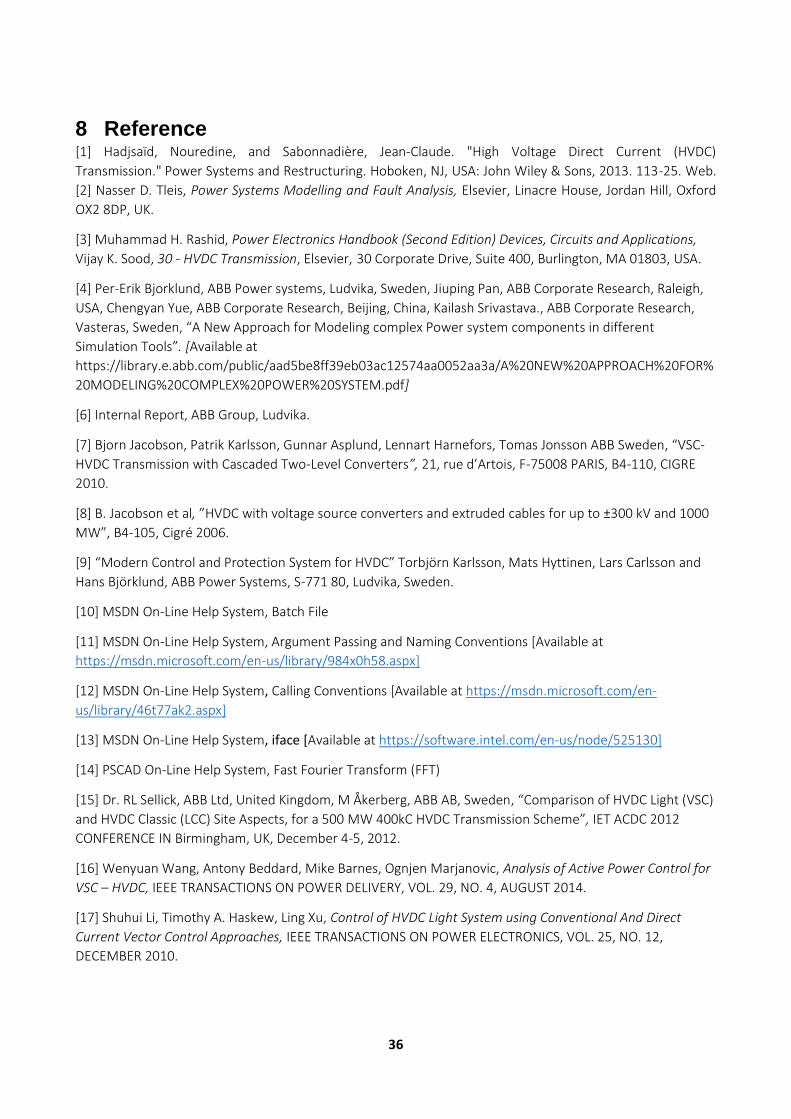
36
8 Reference [1] Hadjsaïd, Nouredine, and Sabonnadière, Jean‐Claude. "High Voltage Direct Current (HVDC)
Transmission." Power Systems and Restructuring. Hoboken, NJ, USA: John Wiley & Sons, 2013. 113-25. Web.
[2] Nasser D. Tleis, Power Systems Modelling and Fault Analysis, Elsevier, Linacre House, Jordan Hill, Oxford
OX2 8DP, UK.
[3] Muhammad H. Rashid, Power Electronics Handbook (Second Edition) Devices, Circuits and Applications,
Vijay K. Sood, 30 - HVDC Transmission, Elsevier, 30 Corporate Drive, Suite 400, Burlington, MA 01803, USA.
[4] Per-Erik Bjorklund, ABB Power systems, Ludvika, Sweden, Jiuping Pan, ABB Corporate Research, Raleigh,
USA, Chengyan Yue, ABB Corporate Research, Beijing, China, Kailash Srivastava., ABB Corporate Research,
Vasteras, Sweden, “A New Approach for Modeling complex Power system components in different
Simulation Tools”. [Available at
https://library.e.abb.com/public/aad5be8ff39eb03ac12574aa0052aa3a/A%20NEW%20APPROACH%20FOR%
20MODELING%20COMPLEX%20POWER%20SYSTEM.pdf]
[6] Internal Report, ABB Group, Ludvika.
[7] Bjorn Jacobson, Patrik Karlsson, Gunnar Asplund, Lennart Harnefors, Tomas Jonsson ABB Sweden, “VSC-
HVDC Transmission with Cascaded Two-Level Converters”, 21, rue d’Artois, F-75008 PARIS, B4-110, CIGRE
2010.
[8] B. Jacobson et al, ”HVDC with voltage source converters and extruded cables for up to ±300 kV and 1000
MW”, B4-105, Cigré 2006.
[9] “Modern Control and Protection System for HVDC” Torbjörn Karlsson, Mats Hyttinen, Lars Carlsson and
Hans Björklund, ABB Power Systems, S-771 80, Ludvika, Sweden.
[10] MSDN On-Line Help System, Batch File
[11] MSDN On-Line Help System, Argument Passing and Naming Conventions [Available at
https://msdn.microsoft.com/en-us/library/984x0h58.aspx]
[12] MSDN On-Line Help System, Calling Conventions [Available at https://msdn.microsoft.com/en-
us/library/46t77ak2.aspx]
[13] MSDN On-Line Help System, iface [Available at https://software.intel.com/en-us/node/525130]
[14] PSCAD On-Line Help System, Fast Fourier Transform (FFT)
[15] Dr. RL Sellick, ABB Ltd, United Kingdom, M Åkerberg, ABB AB, Sweden, “Comparison of HVDC Light (VSC)
and HVDC Classic (LCC) Site Aspects, for a 500 MW 400kC HVDC Transmission Scheme”, IET ACDC 2012
CONFERENCE IN Birmingham, UK, December 4-5, 2012.
[16] Wenyuan Wang, Antony Beddard, Mike Barnes, Ognjen Marjanovic, Analysis of Active Power Control for
VSC – HVDC, IEEE TRANSACTIONS ON POWER DELIVERY, VOL. 29, NO. 4, AUGUST 2014.
[17] Shuhui Li, Timothy A. Haskew, Ling Xu, Control of HVDC Light System using Conventional And Direct
Current Vector Control Approaches, IEEE TRANSACTIONS ON POWER ELECTRONICS, VOL. 25, NO. 12,
DECEMBER 2010.

37
[18] J.L. Kirtley Jr. “Introduction to Power Systems, Class Notes Chapter 4, Introduction to Symmetrical
Components”, Massachusetts Institute of Technology. [Available at http://ocw.mit.edu/courses/electrical-
engineering-and-computer-science/6-061-introduction-to-electric-power-systems-spring-
2011/readings/MIT6_061S11_ch4.pdf]
[20] S.N.Singh, Electric Power Generation, Transmission and Distribution, Asoke K. Ghosh, Prentice-Hall of
India Private Limited, M-97, Connaught Circus, New Delhi – 110001.
[22] J.Arrillaga and N.R. Watson (2001) FACTS and HVDC Transmission, in Computer Modelling of Electrical
Power Systems, Second Edition, John Wiley & Sons, Ltd, West Sussex, England.
doi: 10.1002/9781118878286.ch3
[23] Kim, Chan-Ki, Jang, Gil-Soo, and Sood, Vijay K. HVDC Transmission : Power Conversions Applications in
Power Systems. Hoboken, NJ, USA: John Wiley & Sons, 2009. ProQuest ebrary. Web. 4 February 2016.
[24] Muhammad H. Rashid, Power Electronics Handbook (Second Edition) Devices, Circuits and Applications,
Juan W.Dixon, 12 – Three Phase Controlled Rectifiers, Elsevier, 30 Corporate Drive, Suite 400, Burlington, MA
01803, USA.
[25] Muhammad H. Rashid, Power Electronics Handbook (Second Edition) Devices, Circuits and Applications,
Jose R. Espinoza, 15 - Inverters, Elsevier, 30 Corporate Drive, Suite 400, Burlington, MA 01803, USA.
[26] Branko L. Dokić • Branko Blanuša, Power Electronics Converters and Regulators, Third Edition, Springer
International Publishing, Switzerland.

38
Appendix A

39
Park’s Transformation
Voltage invariant Transformation
The transformation from a stationary phase coordinate to a rotating coordinate system is a space vector
transformation of three phase time domain signals and is often termed as Park’s transform.
[
𝑢𝑑
𝑢𝑞
𝑢0
] =2
3
[ cos (𝜃) cos (𝜃 −
2𝜋
3) cos(𝜃 +
2𝜋
3)
−sin (𝜃) −sin (𝜃 −2𝜋
3) −sin(𝜃 +
2𝜋
3)
1
2
1
2
1
2 ]
[
𝑢𝑎
𝑢𝑏
𝑢𝑐
] = 𝑇 [
𝑢𝑎
𝑢𝑏
𝑢𝑐
] (A.1)
Where, 𝜃 = 𝜔𝑡 + 𝛿𝐴, the angle between the rotating and fixed coordinating system while 𝛿𝐴 is the initial
phase shift of the voltage.
The inverse transformation is given by,
[
𝑢𝑎
𝑢𝑏
𝑢𝑐
] = [
cos (𝜃) −sin (𝜃) 1
cos (𝜃 −2𝜋
3) −sin (𝜃 −
2𝜋
3) 1
cos(𝜃 +2𝜋
3) −sin(𝜃 +
2𝜋
3) 1
] [
𝑢𝑑
𝑢𝑞
𝑢0
] (A.2)
The transforms are same for the current as well. Also 𝑇𝑇−1 = 𝐼, I is the Identity Matrix
Real and Reactive Power
Three phase Real and Reactive power are given by
𝑃 = 3|𝑉| ∗ |𝐼|cos (𝜃)
𝑄 = 3|𝑉| ∗ |𝐼|sin (𝜃)
Where 𝑃(𝑡) is the instantaneous power
𝑈(𝑡) is the instantaneous voltage
𝐼(𝑡) is the instantaneous current
𝜃 is the angle of the phase difference between voltage and current.
The current component which is in phase with the voltage aids the real power. When the voltage and
current are in phase, then 𝜃 becomes zero and P can be expressed as
𝑃 = 𝑣𝑎𝑖𝑎 + 𝑣𝑏𝑖𝑏 + 𝑣𝑐𝑖𝑐
𝑃 = [𝑣𝑎 𝑣𝑏 𝑣𝑐] [
𝑖𝑎𝑖𝑏𝑖𝑐
]
Rewriting the voltage and current matrix in terms of dq0 quantities using the Parks transform,
𝑃 = [𝑣𝑑 𝑣𝑞 𝑣0][𝑇−1]𝑇[𝑇−1] [
𝑖𝑑𝑖𝑞𝑖0
]

40
= [𝑣𝑑 𝑣𝑞 𝑣0]
[ 3
20 0
03
20
0 0 3]
[
𝑖𝑑𝑖𝑞𝑖0
]
𝑃 =3
2(𝑣𝑑𝑖𝑑 + 𝑣𝑞𝑖𝑞 + 2𝑣0𝑖0)
When current and voltage are symmetrical, 𝑣0 ,𝑖0 are zero, Hence
𝑃 =3
2(𝑣𝑑𝑖𝑑 + 𝑣𝑞𝑖𝑞) (A.3)
Similarly the reactive power can be deduced as when 𝜃=90°as the real power becomes zero.
𝑄 = [𝑣𝑎 𝑣𝑏 𝑣𝑐] [
𝑖𝑎𝑖𝑏𝑖𝑐
]
[𝑣𝑎 𝑣𝑏 𝑣𝑐] = [𝑣𝑑 𝑣𝑞 𝑣0][𝑇−1]𝑇
= [𝑣𝑑 𝑣𝑞 𝑣0]
[ cos (𝜃) cos (𝜃 −
2𝜋
3) cos(𝜃 +
2𝜋
3)
sin (𝜃) sin (𝜃 −2𝜋
3) sin(𝜃 +
2𝜋
3)
1 1 1 ]
The current lags the voltage by 𝜋
2 and hence the current is expressed as,
[
𝑖𝑎𝑖𝑏𝑖𝑐
] =
[ cos (𝜃 +
𝜋
2) sin (𝜃 +
𝜋
2) 1
cos (𝜃 −2𝜋
3+
𝜋
2) sin (𝜃 −
2𝜋
3+
𝜋
2) 1
cos (𝜃 +2𝜋
3+
𝜋
2) sin (𝜃 +
2𝜋
3+
𝜋
2) 1]
[
𝑖𝑑𝑖𝑞𝑖0
]
𝑄 = [𝑣𝑑 𝑣𝑞 𝑣0]
[ cos(𝜃) cos (𝜃 −
2𝜋
3) cos (𝜃 +
2𝜋
3)
sin(𝜃) sin (𝜃 −2𝜋
3) sin (𝜃 +
2𝜋
3)
1 1 1 ]
[ cos (𝜃 +
𝜋
2) sin (𝜃 +
𝜋
2) 1
cos (𝜃 −𝜋
6) sin (𝜃 −
𝜋
6) 1
cos (𝜃 +7𝜋
6) sin (𝜃 +
7𝜋
6) 1]
[
𝑖𝑑𝑖𝑞𝑖0
]
𝑄 = [𝑣𝑑 𝑣𝑞 𝑣0]
[ 0
3
20
−3
20 0
0 0 3]
[
𝑖𝑑𝑖𝑞𝑖0
]
𝑄 =3
2(𝑣𝑑𝑖𝑞 − 𝑣𝑞𝑖𝑑 + 2𝑣0𝑖0)
When current and voltage are symmetrical, 𝑣0 ,𝑖0 are zero, Hence
𝑄 =3
2(𝑣𝑑𝑖𝑞 − 𝑣𝑞𝑖𝑑) (A.4)

41
RMS voltages
The phase voltages can be expressed in terms of RMS as,
𝑣𝑎 = √2𝑉𝑟𝑚𝑠 cos(𝜔𝑡)
𝑣𝑏 = √2𝑉𝑟𝑚𝑠cos (𝜔𝑡 −2𝜋
3)
𝑣𝑐 = √2𝑉𝑟𝑚𝑠cos (𝜔𝑡 +2𝜋
3)
We know,
[
𝑣𝑑
𝑣𝑞
𝑣0
] =2
3
[ cos(𝜃) cos (𝜃 −
2𝜋
3) cos (𝜃 +
2𝜋
3)
− sin(𝜃) − sin (𝜃 −2𝜋
3) −sin (𝜃 +
2𝜋
3)
1
2
1
2
1
2 ]
[
𝑣𝑎
𝑣𝑏
𝑣𝑐
]
[
𝑣𝑑
𝑣𝑞
𝑣0
] =2
3
[ cos(𝜃) cos (𝜃 −
2𝜋
3) cos (𝜃 +
2𝜋
3)
− sin(𝜃) − sin (𝜃 −2𝜋
3) −sin (𝜃 +
2𝜋
3)
1
2
1
2
1
2 ]
[ √2𝑉𝑟𝑚𝑠 cos(𝜔𝑡)
√2𝑉𝑟𝑚𝑠 cos (𝜔𝑡 −2𝜋
3)
√2𝑉𝑟𝑚𝑠 cos (𝜔𝑡 +2𝜋
3)]
[
𝑣𝑑
𝑣𝑞
𝑣0
] =2
3√2𝑉𝑟𝑚𝑠
[ 3
2cos(𝜃 − 𝜔𝑡)
3
2sin(𝜃 − 𝜔𝑡)
0 ]
[
𝑣𝑑
𝑣𝑞
𝑣0
] = √2𝑉𝑟𝑚𝑠 [cos(𝜃 − 𝜔𝑡)
sin(𝜃 − 𝜔𝑡)0
] (A.5)
It can also be written as,
√𝑣𝑑2 + 𝑣𝑞
2 = √2𝑉𝑟𝑚𝑠 (A.6)

42
Appendix B

43
Model Parameters
Rated Power 390 [MVA]
PCC Bus Voltage 132 [kV]
Converter Bus Voltage 195 [kV]
Base AC Voltage 195 [kV]
Nominal DC Voltage 150 [kV]
Base Frequency 50 [Hz]
DC Line Resistance 3.08142 [ohm]
Reactor Inductance 0.0389000
Transformer Base Power 390 [MVA]

44
Appendix C
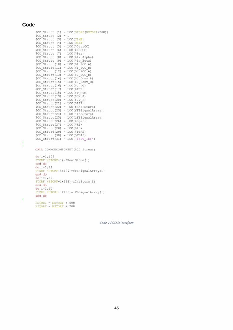
45
Code
$CC_Struct (1) = LOC(STORI(NSTORI+200))
$CC_Struct (2) = 1
$CC_Struct (3) = LOC(TIME)
$CC_Struct (4) = LOC(DELT)
$CC_Struct (5) = LOC($CtrlCC)
$CC_Struct (6) = LOC($REFCC)
$CC_Struct (7) = LOC($Par)
$CC_Struct (8) = LOC($Iv_Alpha)
$CC_Struct (9) = LOC($Iv_Beta)
$CC_Struct(10) = LOC($I_PCC_A)
$CC_Struct(11) = LOC($I_PCC_B)
$CC_Struct(12) = LOC($U_PCC_A)
$CC_Struct(13) = LOC($U_PCC_B)
$CC_Struct(14) = LOC($U_Conv_A)
$CC_Struct(15) = LOC($U_Conv_B)
$CC_Struct(16) = LOC($U_DC)
$CC_Struct(17) = LOC($TFR)
$CC_Struct(18) = LOC($P_nom)
$CC_Struct(19) = LOC($Uv_A)
$CC_Struct(20) = LOC($Uv_B)
$CC_Struct(21) = LOC($ITR)
$CC_Struct(22) = LOC(fRealStore)
$CC_Struct(23) = LOC(fFBSignalArray)
$CC_Struct(24) = LOC(iIntStore)
$CC_Struct(25) = LOC(iFBSignalArray)
$CC_Struct(26) = LOC($Opar)
$CC_Struct(27) = LOC($RS)
$CC_Struct(28) = LOC($IS)
$CC_Struct(29) = LOC($FBRS)
$CC_Struct(30) = LOC($FBIS)
$CC_Struct(31) = LOC('$(ST_ID)')
!
!
CALL COMMONCOMPONENT($CC_Struct)
do i=1,109
STORF(NSTORF+i)=fRealStore(i)
end do
do i=1,14
STORF(NSTORF+i+109)=fFBSignalArray(i)
end do
do i=1,60
STORF(NSTORF+i+123)=iIntStore(i)
end do
do i=1,10
STORI(NSTORI+i+183)=iFBSignalArray(i)
end do
!
NSTORI = NSTORI + 500
NSTORF = NSTORF + 200
Code 1 PSCAD Interface

46
typedef struct CC_Interface
{
char *memory;
float firststep;
double *time;
double *timestep;
double *ctrl_cc;
double *ref_cc;
double *par;
double *IvAlpha; // Input Measurement (in pu of IBase = (1/KiPu) )
double *IvBetapu; // Input Measurement (in pu of IBase = (1/KiPu) )
double *IprimAlphapu; // Input , measurement in pu
double *IprimBetapu; // Input , measurement in pu
double *UpccAlphapu; // Input , measurement in pu of UPrimBas
double *UpccBetapu; // Input , measurement in pu of UPrimBas
double *UconvAlphapu; // Input, measurement in pu of UBase
double *UconvBetapu; // Input, measurement in pu of UBase
double *Udpu; // Input Measurement, 0.5*(UdpKv -UdnKv)*KuPu
(i.e.measured in pu of UBase)
double *tfr;
double *pnom;
double *UvOutAlfa;
double *UvOutBeta;
double *itr;
double *fRealStore; // Real states, to tbe stored to next timestep
double *fFBSignalArray; // Integer states, to tbe stored to next timestep
double *iIntStore; // double Feedback signals array
double *iFBSignalArray; // Integer Fedback signals array
double *OptionalParam; // Parameter, Real Optional user defined parameters
recommended by ABB, default=0
double *NumberOfRealStates; // Number of real state variables
double *NumberOfIntegerStates; // Number of integer state variables
double *NumberOfFBRealStates; // Number of real state Feed back variables
double *NumberOfFBIntegerStates; // Number of integer state Feed back variables
char *sConverterId; // Character Parameter/Identifiers
}CC_Interface;
void COMMONCOMPONENT(CC_Interface *x);
Code 2 : C++ interface

47
self.IvQOrd = x->tfr[3];
self.IvDRef = x->tfr[4];
self.IvQRef = x->tfr[5];
self.Overmod = x->itr[0];
self.UvOutAbsMax = x->tfr[6];
self.ChopperOnP = x->itr[1];
self.ChopperOnN = x->itr[2];
self.EChop = x->itr[3];
self.UvOutAlfa = (*x->UvOutAlfa);
self.UvOutBeta = (*x->UvOutBeta);
if (time==0.0f)
{
self.iInspectFileOpen = 0;
s = x->par[6];
}
Else
{
self.iInspectFileOpen = x->par[15];
s = fs;
}
ABB_HVDC_LIGHT_CONVERTER_V2_0(&isw, ×tep, &s, &InitMethodUd, &self, &time, &ConvNr);
//Plotting:
x->tfr[7] = self.ModIndex;
x->tfr[0] = self.PPcc;
x->tfr[1] = self.QPcc;
x->tfr[2] = self.IvDOrd;
x->tfr[3] = self.IvQOrd;
x->tfr[4] = self.IvDRef;
x->tfr[5] = self.IvQRef;
x->itr[0] = self.Overmod;
x->itr[1] = self.ChopperOnP;
x->itr[2] = self.ChopperOnN;
Code 3 Calling Common Component from interface

48
using namespace std;
void ABB_HVDC_LIGHT_CONVERTER_V2_0(int *iswx,float *fInternalStepx,int *iCalcModex, int
*InitMethodUdc, ConverterDataDef *conv, float *fInternalTimex, int *ConvNrx)
{
//ConvNr is just for debuuging.
// See Comment labeled Lars for changed data
char* strLight_ConverterVersionString="Abb_Hvdc_Light_Converter_V2.0";
static FILE *pfiles[20];
int isw=*iswx; // Is =1 first time in each external step
int ConvNr=*ConvNrx;
float fInternalStep=(float) *fInternalStepx; // Shall be changed to double whe all fortran routines
accepts double as argument
double fInternalTime= *fInternalTimex;
int iCalcMode=*iCalcModex;
char* sErrorMessage=conv->sErrorMessage;
int InitMethodUd= *InitMethodUdc;
int iAutoInitLoadFlow=0;
float DummyForPlots[iRealPlotMaxConv+1];
Code 4 Common Component Main file


TRITA TRITA-EE 2016:055
www.kth.se