DEVELOPMENT OF DRY AND EVAPORATIVE FLUID...

DEVELOPMENT OF DRY AND EVAPORATIVE

FLUID COOLER MODELS FOR ENERGYPLUS

By

CHANDAN SHARMA

Bachelor of Engineering

SGS Institute of Technology and Science

Indore, MP, India

2007

Submitted to the Faculty of the Graduate College of the

Oklahoma State University in partial fulfillment of the requirements for

the Degree of MASTER OF SCIENCE

December, 2009

ii

DEVELOPMENT OF DRY AND EVAPORATIVE

FLUID COOLER MODELS FOR ENERGYPLUS

Thesis Approved:

Dr. D. E. Fisher

Thesis Adviser

Dr. J. D. Spitler

Dr. Lorenzo Cremaschi

Dr. A. Gordon Emslie

Dean of the Graduate College

iii

ACKNOWLEDGMENTS

It would be really impossible for me to express my gratitude for all those people who

have helped me directly or indirectly to achieve this goal but I’ll give it try.

My first and foremost thanks go to my mother. It is her selfless love and affection that

made me strong enough to face the difficult moments of life. I truly owe all my past, present

and future successes to her because without her contribution on my foundation nothing was

ever possible. I thank my father to inculcate values, discipline and diligence in me. My

younger sister always had and will have a special place in my life. I still enjoy the cute

moments shared with her in childhood. Those silly activities, fights, cry are a great source of

our happiness now. As we grew up, she always provided the support to me whenever needed.

I love her a lot and wish her all the good luck for the great life ahead.

My school teachers played a crucial part in my life. Thankfully, I was very fortunate

to have great teachers in my life. There are many to name but I would specially like to thank

Dr. Pandey, Dr. Ambekar, Dr. Aasif, Mr. Tripathi, Mr. Pawar and Mr. Ajay Garg for all their

teachings and blessings.

Working with Dr. Fisher was like a gift to me. I learnt so much about so many things

from him. His ever smiling face, attitude towards life, great subject knowledge and helping

nature for every one make him an outstanding person. This thesis couldn’t be finished

without his guidance and support in tough times. I would like to express my gratitude for Dr.

iv

Spitler and Dr. Cremaschi. Dr. Spitler’s class was a turning point in my graduate

school career. His great subject knowledge, sense of perfection, punctuality and discipline

are really admirable. His class equipped me to become a better HVAC professional in many

ways. He along with Dr. Fisher and Dr. Ghajar helped me to build the foundation on which I

later developed my HVAC expertise.

Special thanks to Sankar, Edwin, Ellisa, Ehsan, Pranav, James, Kaustubh and Malai

for all their support throughout. I could never achieve what I achieved without their help. My

best wishes to all of them for their bright future and prosperous life.

v

TABLE OF CONTENTS

Chapter Page

1. INTRODUCTION .....................................................................................................1

1.1 Background ........................................................................................................1

1.2 Objectives ..........................................................................................................5

2. LITERATURE REVIEW ..........................................................................................6

2.1 Evaporative fluid cooler models ........................................................................6

2.1.1 Zalewski and Gryglaszewski (1997) ........................................................6

2.1.2 Hasan and Siren (2002) ............................................................................9

2.1.3 Lebrun et al. (2004) ................................................................................12

2.1.4 Stabat and Marchio (2004)) ...................................................................15

2.1.5 Quereshi and Zubair (2005) ..................................................................19

2.2 Dry fluid cooler models ...................................................................................22

2.2.1 LMTD method .......................................................................................22

2.2.2 ℇ-NTU method .......................................................................................23

3. MODEL DEVELOPMENT .....................................................................................25

3.1 Overview of the models ...................................................................................25

3.2 EnergyPlus model description .........................................................................27

3.3 Implementing the fluid cooler model in EnergyPlus .......................................30

vi

3.3.1 Input specification of fluid cooler models ....................................................31

3.3.2 Implementation algorithm of fluid cooler models ........................................33

4. PERFORMANCE EVALUATION OF FLUID COOLER MODELS ....................42

4.1 Model sensitivity to input parameters ..............................................................43

4.1.2 Methodology ...........................................................................................44

4.1.3 Sensitivity of UA for change in design parameters ................................44

4.2 Parametric study with different set-point temperatures ...................................46

4.3 Parametric study at different locations ............................................................48

4.4 Summary ..........................................................................................................50

5. MODEL VERIFICATION ......................................................................................52

5.1 Evaporative fluid cooler: comparison with published data sets .......................52

5.2 Dry fluid cooler: EnergyPlus and HVACSIM+ models ..................................55

5.3 Evaporative fluid cooler: EnergyPlus and Lebrun ...........................................58

5.4 Summary of results ..........................................................................................59

6. MODEL IMPLEMENTATION VERIFICATION..................................................61

6.1 The EnergyPlus models ...................................................................................61

6.2 Example building and system description .......................................................63

6.3 Design day building load profile......................................................................64

6.4 Dry fluid cooler configuration .........................................................................65

6.4.1 Series configuration ...............................................................................66

6.4.2 Parallel configuration .............................................................................70

6.5 Evaporative fluid cooler configuration ............................................................74

6.5.1 Series configuration ...............................................................................74

vii

6.5.2 Parallel configuration .............................................................................78

7. CONCLUSION AND RECOMMENDATION ......................................................81

REFERENCES ............................................................................................................84

APPENDIX A Parametric study of varying dry-bulb temperature in evaporative fluid

cooler model .......................................................................................86

APPENDIX B Description of VBA implementation of Lebrun model .......................91

viii

LIST OF TABLES

Table Page

2.1 ℇ-NTU relations for wet and dry regimes ...........................................................16

4.1 UA sensitivity for dry fluid cooler ......................................................................45

4.2 UA sensitivity for evaporative fluid cooler ........................................................45

4.3 Dry fluid cooler fan energy sensitivity with respect to UA: different setpoints .46

4.4 Evap fluid cooler fan energy sensitivity with respect to UA: different setpoints47

5.1 Catalog data for Baltimore Aircoil closed circuit cooling tower ........................53

5.2 Input parameters of HVACSIM+ and EnergyPlus dry fluid cooler models .......57

5.3 Parameters estimation results of Lebrun model ..................................................58

A-1 Parametric study of varying dry-bulb temperature for evap fluid cooler ..........87

ix

LIST OF FIGURES

Figure Page

1.1 Schematic of dry fluid cooler ................................................................................2

1.2 Schematic of evaporative fluid cooler ..................................................................3

1.3 Dry fluid cooler and Evaporative fluid cooler ......................................................4

2.1 Heat exchange scheme of Zalewski and Gryglaszewski (1997) ...........................7

2.2 Heat exchange scheme of Stabat and Marchio (2004) ........................................15

3.1 Baltimore Aircoil’s catalog data for evaporative fluid coolers ...........................26

3.2 Motivair corp. catalog data for dry fluid coolers ................................................27

3.3 Flow chart: UA method of fluid cooler in EnergyPlus .......................................28

3.4 Flow chart: Design Capacity method of fluid cooler in EnergyPlus ..................29

3.5 Flow chart: UA calculation method in EnergyPlus ............................................30

3.6 IDD file for dry fluid cooler................................................................................32

3.7 IDF file for dry fluid cooler ................................................................................33

4.1 Dry fluid cooler fan energy sensitivity with respect to UA: different locations .49

4.2 Evap fluid cooler fan energy sensitivity with respect to UA: different locations49

x

Figure Page

5.1 Catalogue data Vs EnergyPlus capacity .............................................................54

5.2 EnergyPlus Vs HVACSIM+ capacity .................................................................58

5.3 EnergyPlus Vs Lebrun model capacity ...............................................................59

6.1 EnergyPlus loop diagram ....................................................................................62

6.2 Isometric and plan views of the building ............................................................64

6.3 Plant loop cooling demand for design day ..........................................................65

6.4 Single dry fluid cooler: heat transfer rates ..........................................................66

6.5 Dry fluid cooler: Series configuration I ..............................................................68

6.6 Out side air dry-bulb and loop outlet temperature ..............................................69

6.7 Dry fluid cooler: Series configuration II .............................................................70

6.8 Dry fluid cooler: Parallel configuration I............................................................71

6.9 Out side air dry-bulb and loop outlet temperature ..............................................72

6.10 Dry fluid cooler: Parallel configuration II ........................................................73

6.11 Single evaporative fluid cooler: heat transfer rates ...........................................74

6.12 Evaporative fluid cooler: Series configuration I ...............................................76

6.13 Out side air wet-bulb and loop outlet temperature ............................................76

6.14 Evaporative fluid cooler: Series configuration II..............................................77

6.15 Evaporative fluid cooler: Parallel configuration I ............................................79

6.16 Out side air wet-bulb and loop outlet temperature ............................................79

6.17 Evaporative fluid cooler: Parallel configuration I ............................................80

B-1 Flow chart of Lebrun model implemented in VBA ...........................................92

xi

NOMENCLATURE

m� = Mass flow rate (kg/s)

C� = Capacity flow rate W/K

h = Enthalpy (j/kg-K)

T = Temperature (°C) or (K)

c� = Specific heat (j/kg-K)

R = Resistance (K/W)

W = Humidity ratio ((kgw / kgdryair))

Le = Lewis number

Φ = Relative humidity

U = Fluid cooler overall heat transfer coefficient, W/m2- oC

A = Heat transfer surface area, m2

Subscripts

a = Air

w = Water

p = Process fluid

wb = Wet-bulb

in = Inlet

xii

out = Outlet

�ic = Fictitious

db = Dry-bulb

spray = Spray water for evaporative fluid cooler

1

CHAPTER I

INTRODUCTION

1.1 Background

Dry fluid coolers and evaporative fluid coolers provide a clean and effective method

of cooling the process fluid. Fig 1.1 and 1.2 show the schematics of dry and evaporative fluid

coolers respectively. The process fluid which is generally water or water/glycol mixture is

circulated in the closed loop and the ambient air passes across the coil. In the case of dry

fluid coolers only air is used to cool the process fluid while in the case of evaporative fluid

coolers spray water is used along with ambient air to enhance the effectiveness of the heat

exchanger. Because of the usage of spray water, evaporative fluid cooler can cool fluid up to

wet-bulb temperature of air. Dry fluid coolers can cool fluid to ambient air dry-bulb

temperature.

Dry fluid coolers are combination of outside fan cooled heat exchanger and a

pumping station. The process fluid (water/glycol solution) which is used to cool the

equipment is circulated by the pump between the heat exchanger and the equipment. Because

2

of the same fluid circulation, internal scaling and corrosion are virtually eliminated. Unlike

cooling towers, dry fluid coolers cool the process fluid without any evaporation loss, water

treatment or routine maintenance. Some of the dry fluid coolers switch to adiabatic mode in

hot climate where the ambient temperatures are very high to provide sufficient fluid cooling.

In the adiabatic mode, a fine mist of water is added in the air before it gets in contact with the

coil circulating the fluid.

Fig 1.1 Schematic of dry fluid cooler

Water evaporates before coming in contact with the coil and corrosion and scale

formation are prevented. The dry fluid cooler has been widely used in both the US and

Europe for many years and the installed base of dry fluid coolers is very large.

Process fluid

Heated Air

Air In Air In

Air

(ma, tdb,out)

(mw, tw,out)

(ma, tdb,in)

(mw, tw,in)

3

Another way of cooling the process fluid can be cooling towers. There are two types

of cooling towers: open circuit cooling tower and closed cooling tower. Open circuit cooling

tower also known as direct contact cooling tower cool the fluid by exposing it to outside air

directly. Because of the direct contact with the air, water becomes contaminated. Water

treatment, regular heat-exchanger cleaning, difficult cold-weather operation, and large

consumption of water are some of the disadvantages of direct contact cooling tower.

Fig 1.2 Schematic of evaporative fluid cooler

Process fluid

Drift eliminatorsHeated Air

Spray distribution

Air In

Pump

Air In

Water Air

External water

(ma, ha,out)

(mw, tw,out) (ma, twb,in)

(mw, tw,in)

On the other hand closed circuit cooling tower cool the process fluid by circulating

them in a closed loop. They require very less maintenance as compare to open circuit cooling

towers. Closed circuit cooling towers are also called as indirect contact cooling towers

(ICCTs), evaporative fluid/liquid/water

closed wet towers. Open circuit cooling towers have been used in the industry for more than

eight decades but now dry fluid coolers and closed circuit towers are replacing them more

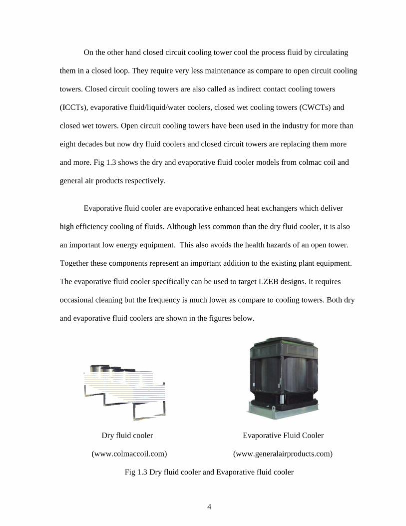
and more. Fig 1.3 shows the dry and evaporative fluid cooler models from colmac coil and

general air products respectively.

Evaporative fluid cooler are evaporative enhanced heat exchangers which deliver

high efficiency cooling of fluids.

an important low energy equipment

Together these components represent an important addition to the existing plant equipment.

The evaporative fluid cooler specifically

occasional cleaning but the frequency is much lower as compare to c

and evaporative fluid coolers are shown in the figures below.

Dry fluid cooler

(www.colmaccoil.com)

Fig 1.3 Dry fluid cooler and Evaporative fluid cooler

4



uit cooling towers are also called as indirect contact cooling towers

/liquid/water coolers, closed wet cooling towers (CWCTs)

Open circuit cooling towers have been used in the industry for more than

ecades but now dry fluid coolers and closed circuit towers are replacing them more

Fig 1.3 shows the dry and evaporative fluid cooler models from colmac coil and

general air products respectively.


high efficiency cooling of fluids. Although less common than the dry fluid cooler, it

equipment. This also avoids the health hazards of an open


The evaporative fluid cooler specifically can be used to target LZEB designs

cleaning but the frequency is much lower as compare to cooling towers.

and evaporative fluid coolers are shown in the figures below.

Dry fluid cooler Evaporative Fluid Cooler

(www.colmaccoil.com) (www.generalairproducts.com)

Dry fluid cooler and Evaporative fluid cooler



uit cooling towers are also called as indirect contact cooling towers

(CWCTs) and

Open circuit cooling towers have been used in the industry for more than

ecades but now dry fluid coolers and closed circuit towers are replacing them more

Fig 1.3 shows the dry and evaporative fluid cooler models from colmac coil and


ommon than the dry fluid cooler, it is also

health hazards of an open tower.


LZEB designs. It requires

ooling towers. Both dry

Evaporative Fluid Cooler

(www.generalairproducts.com)

5

1.2 Objectives

The main objectives of this study are as follows:

1) Obtain information about existing dry and evaporative fluid cooler models through

literature review

2) Develop and implement dry and evaporative fluid cooler models in EnergyPlus. The

models are added as two new modules in EnergyPlus environment. .

3) Determine sensitivity of the model with respect to various inputs.

4) Provide user documentation for EnergyPlus which states the inputs and outputs of the

model. The document also discusses the reference model and how it works in

EnergyPlus

5) Verify EnergyPlus model by using other available fluid cooler models and determine

the quality of the results.

6

CHAPTER II

LITERATURE REVIEW

In this chapter, a review of existing models of fluid coolers will be presented. The

accuracy, range of applicability and simplicity of the models are discussed. Also the issues

pertaining to implementation of models in building simulation programs are discussed e.g.

availability of input parameters, convergence problems etc. Finally a summary of the

findings is presented in the last section of the chapter.

2.1 Evaporative fluid cooler models

2.1.1 Zalewski and Gryglaszewski (1997) – Mathematical model of heat and mass

transfer processes in evaporative fluid coolers

Zalewski and Gryglaszewski (1997) presented the mathematical model of evaporative

fluid cooler by using four ordinary differential equations with their associated boundary

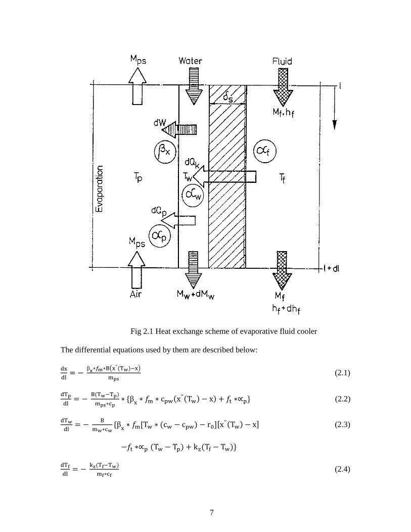
conditions and some algebraic equations. Fig 2.1 shows the schematic of the evaporative

fluid cooling process modeled by them.

7

Fig 2.1 Heat exchange scheme of evaporative fluid cooler

The differential equations used by them are described below:

�� β�� !�"#�′′$%&'(�)

*+, (2.1)

�%+�� "$%&(%+'

*+,�-+� .β� � /* � c�0$x′′$T0' � x' 2 /3 �4�5 (2.2)

�%&�� "

*&�-&.β� � /*6T0 � $c0 � c�0' � r896x′′$T0' � x9 (2.3)

�/3 �4� $T0 � T�' 2 k;$T< � T0'5 �%=�� >?$%=(%&'

*=�-= (2.4)

8

The boundary conditions for the equations (2.1)-(2.4) are as follows:

x$L' � x@; T�$L' � T�x@; T0$0' � T0$L' And T<$0' � T<@

Where,

x = air humidity ratio (kgw kgps-1)

l = length, linear coordinate, (m)

β� = mass transfer coefficient, (kgps m-2 s-1)

/, /3, /* = area ratio

B = length of wall, length of tubes of exchanger, (m)

T = temperature (°C)

4 = heat transfer coefficient (W m-2 K-2)

r8 = latent heat of vaporization at 0°C; r8 = 2500800 (J kg-1)

h = specific enthalpy (J kg-1)

W= mass flow rate of water vapor (kg s-1)

Qk = heat flux through wall (W)

Qp = heat flux from water surface into air (W)

E = thickness, (m)

c = specific heat at constant pressure (J kg-1 K-1)

Subscripts

ps = dry air

pw = water vapor

f = cooled liquid

9

p = moist air

w = spraying water

1= inlet (initial) value

2= final (outlet) value

s = wall

′′ = saturation state

The model heavily depends on the specification of the geometry of evaporative fluid

cooler which is mostly not available in manufacturer’s catalog data. Also, spray water

temperature input parameter required by the model is not available in the catalog data. Along

with these, determination of heat and mass transfer coefficient is very difficult. Because of

the reasons stated above, the model is not suitable for implementing into the building energy

simulation programs.

2.1.2 Hasan and Siren (2002) – Theoretical and computational analysis of closed wet

cooling towers

Hasan and Siren (2002) presented the theoretical analysis and computation modeling

of closed wet cooling towers. They defined tower heat and mass transfer coefficient by using

experimental measurements of a prototype of 10 KW tower. They divided the cooling tower

tube coils into small elements along the height of the tower. Then heat and mass transfer are

considered for each element, starting from first element at cooling water inlet and then

proceeding along cooling water flow.

The energy and mass balance equations used in the model are shown below.

10

The rate of heat lost by the cooling tower dq- is

dq- � �UH$T- � TI'dA (2.5)

Heat transfer rate from water-air interface to air stream is given by

dqK � mKdhK � k$hIL � hK'dA (2.6)

Total energy balance for an element is given by

m-C0dT- 2 mKdhK 2 mIC0dTI � 0 (2.7)

The inlet spray water temperature is assumed to be equal to the outlet spray water

temperature. So,

TI@ � TIM (2.8)

And finally the mass balance for the element is given by

mN � mKdWK � k$WIL � WK'dA (2.9)

Where,

q = Rate of heat transfer (W)

T = Temperature (°C)

A = Area (m2)

C = specific heat capacity (kJ/kg-K)

h = Enthalpy (kJ/kg)

W = humidity ratio of moist air (kg water/kg dry air)

m = mass flow rate (kg/s)

k = mass transfer coefficient (kg/s-m2)

subscripts

11

c=cooling water

a = air

s= spray water

1 = inlet to tower

2 = outlet to tower

e = evaporation.

superscript

O = saturated condition

There are eight simulation variables which are inlet and outlet values of TI, T-, hK and WK and

3 model input parameters which areT-@, hK@ and WK@. The mass transfer coefficient, which

must be specified at the beginning of the simulation, is calculated as follows

k � 0.065 GK8.TTU (2.10)

Where,

GK = air mass velocity based on minimum section (Kg s-1 m-2)

Eq (2.10) is applicable for 0.96 W XK W 2.76 (Kg s-1 m-2).

The mass transfer coefficient correlation (2.10) is developed for a particular prototype and is

not a generally applicable for all the evaporative fluid cooler models. Getting the humidity

ratio as the input parameter is very difficult as none of the manufacturers provide it in their

catalogs.

12

2.1.3 Lebrun et al. (2004) - Simplified model

Lebrun et al. (2004) applied a unified theoretical treatment to both evaporative heat

exchangers and cooling towers. They regarded these direct and indirect contact cooling

towers as classical heat exchangers working in wet regime. The main difference in the model

was related to different global heat transfer coefficient for each type.

The mathematical model used by them is described below:

The air side energy balance is

Q� � m� K#hK,\]3 � hK,^_) (2.11)

Using the fictitious gas assumption, this equation can be expressed as

Q� � C� K<#T0`,\]3 � T0`,^_) (2.12)

C� K�^- � mK� c�,K�^- (Fictitious capacity of humid air) (2.13)

By using equations (2.11), (2.12) and (2.13):

c�,K�^-= #ab,cde(ab,fg)

#%&h,cde(%&h,fg)

The heat flow rate is calculated by:

Q� � ℇ�^-C� *^_$T0,^_ � T0`,^_' (2.14)

And the process fluid side energy balance is:

Q� � C� 0$T0,^_ � T0`,^_' (2.15)

C� 0 = m� 0c�,0 (Capacity of process fluid) (2.16)

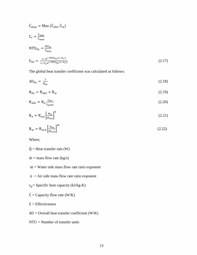
The step by step method to calculate effectiveness of the heat exchanger is described below:

C� *^_ � Min $C� K�^-, C� 0'

13

C� *K� � Max $C� K�^-, C� 0'

Cj � k� !fgk� !b�

NTU�^- � mn�fok� !fg

ℇ�^- � @(N$pqrs�fo$tpuv''@(kvN$pqrs�fo$tpuv'' (2.17)

The global heat transfer coefficient was calculated as follows:

AU�^- � @w�fo

(2.18)

R�^- � RK�^- 2 R0 (2.19)

RK�^- � RK-+,b

-+,b�fo (2.20)

RK � RK,_ x *� b*� b,g

y_ (2.21)

R0 � R0,_ x *� &*� &,g

y*

(2.22)

Where,

Q� = Heat transfer rate (W)

m� = mass flow rate (kg/s)

m = Water side mass flow rate ratio exponent

n = Air side mass flow rate ratio exponent

c�= Specific heat capacity (kJ/kg-K)

C� = Capacity flow rate (W/K)

ℇ = Effectiveness

AU = Overall heat transfer coefficient (W/K)

NTU = Number of transfer units

14

R = Resistance (K/W)

subscripts

a = air

w = water

n= nominal

fic = fictitious

in = inlet

out = outlet

min = minimum

max = maximum

r = ratio

wb = wet-bulb

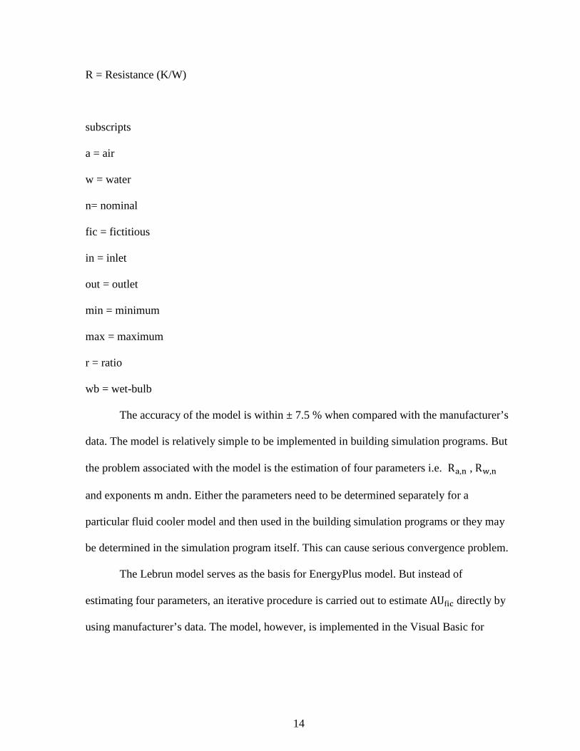
The accuracy of the model is within ± 7.5 % when compared with the manufacturer’s

data. The model is relatively simple to be implemented in building simulation programs. But

the problem associated with the model is the estimation of four parameters i.e. RK,_ , R0,_

and exponents m andn. Either the parameters need to be determined separately for a

particular fluid cooler model and then used in the building simulation programs or they may

be determined in the simulation program itself. This can cause serious convergence problem.

The Lebrun model serves as the basis for EnergyPlus model. But instead of

estimating four parameters, an iterative procedure is carried out to estimate AU�^- directly by

using manufacturer’s data. The model, however, is implemented in the Visual Basic for

15

Application for the verification of EnergyPlus model. All the four parameters are estimated

in VBA program.

2.1.4 Stabat and Marchio (2004) - Simplified model

Another simplified model was presented by Stabat and Marchio (2004) for indirect

contact evaporative cooling towers. ℇ-NTU method is used to describe the model. Fig 2.2

shows the heat exchange scheme used in the model. The scheme consisted of two parts, 1)

heat transfer between air and water film outside the tube; and 2) heat transfer between water

in the tubes and water film outside the tube.

Fig 2.2 Heat transfer scheme of closed circuit cooling tower

These heat transfers are characterized by air and water side heat transfer coefficients

respectively. Finally the overall heat transfer coefficient is used to represent heat transfer

between water and air. Closed cooling towers are also operated without spray when the

16

atmospheric conditions are favorable. So depending on whether the operation is with or

without spray, closed circuit cooling towers operate in wet and dry regimes respectively.

Table 2.1 shows the equations used to calculate overall heat transfer coefficient of counter

flow single pass heat exchanger for both dry and wet regimes.

Table 2.1 - ℇ-NTU relations for wet and dry regimes

Wet regime Dry regime

ℇ � k� &$%&,fg(%&,cde'k� !fg$%&,fg(%b,fg' ℇ � k� &$%&,fg(%&,cde'

k� !fg$%&,fg(%b,fg'

ℇ � @(N$pqrs$tpuv''@(kvN$pqrs$tpuv'' (if Cj W 1 ) with NTU � neme

k� !fg and Cj � k� !fg

k� !b�

ℇ � {%n@|{%n (if Cj � 1 )

C� K � m� Kc�,IK3 and C� 0 = m� 0c�,0 C� K � m� Kc�K and C� 0 = m� 0c�,0

C� *K� � Max $C� K, C� 0' ; C� *^_ � Min $C� K, C� 0' and c�,IK3 � #ab,cde(ab,fg)#%&h,cde(%&h,fg)

@neme

� @n}�e&}em}�e 2 @

nfge&}emfge

@neme

� @n}�e

~v�m}�e 2 @nfge

~v�mfge

Where,

ℇ = Effectiveness;


C� = Capacity flow rate (W K-1)

c� � Specific heat (J kg-1 K-1)

c�,IK3 � Fictitious specific heat (J kg-1 K-1)

m� � Mass flow rate (kg s-1)

17

h = Enthalpy (J kg-1)

AN�3, A^_3 � Surface area at external and internal side (m2)

UN�30N3, UN�3�j� � Air side heat transfer coefficient in wet and dry regime (W K-1m-2)

U^_30N3, U^_3�j� � Water side heat transfer coefficient in wet and dry regime (W K-1 m-2)

U3A3 = Overall heat transfer coefficient (W K-1)

NTU = Number of Transfer units

Subscripts

w = water

a = air

in = inlet

out = outlet

t = total

wb = wet-bulb

r = ratio

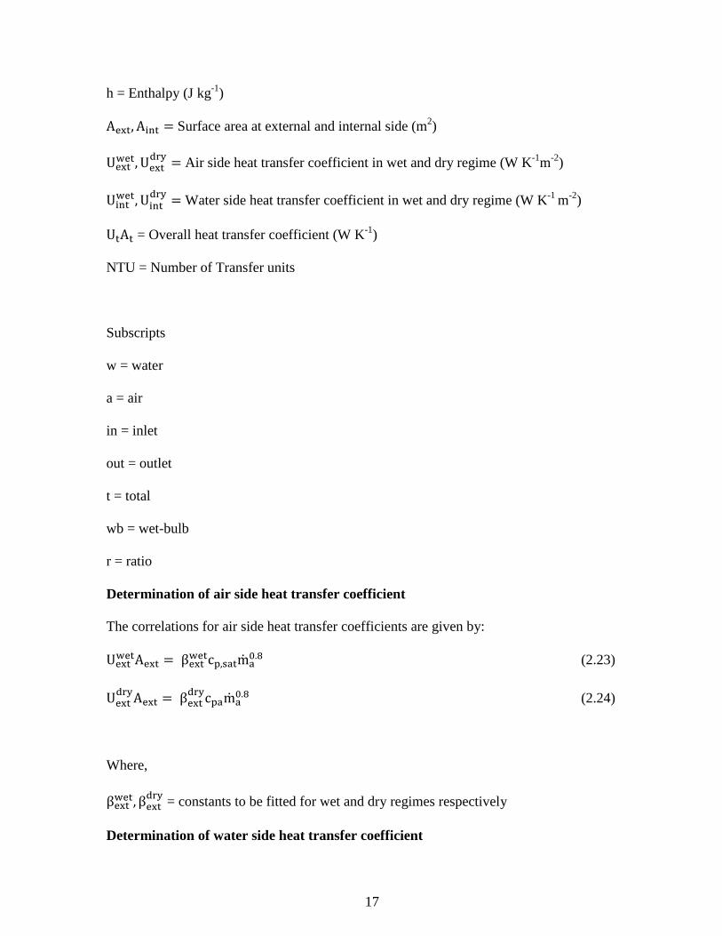
Determination of air side heat transfer coefficient

The correlations for air side heat transfer coefficients are given by:

UN�30N3AN�3 � βN�30N3c�,IK3m� K8.� (2.23)

UN�3�j�AN�3 � βN�3

�j�c�Km� K8.� (2.24)

Where,

βN�30N3, βN�3�j� = constants to be fitted for wet and dry regimes respectively

Determination of water side heat transfer coefficient

18

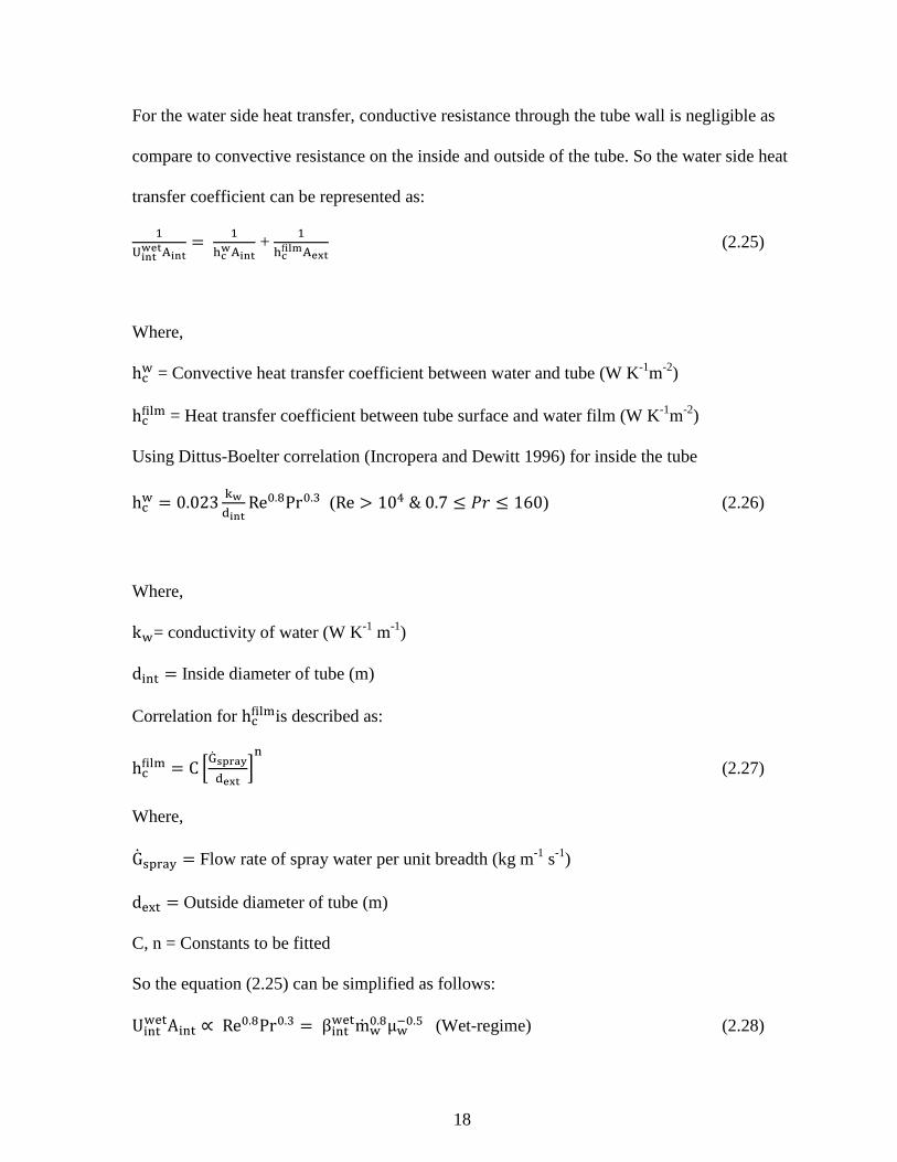
For the water side heat transfer, conductive resistance through the tube wall is negligible as

compare to convective resistance on the inside and outside of the tube. So the water side heat

transfer coefficient can be represented as:

@nfge&}emfge

� @ao&mfge

+ @ao�f�!m}�e

(2.25)

Where,

h-0 = Convective heat transfer coefficient between water and tube (W K-1m-2)

h-�^�* = Heat transfer coefficient between tube surface and water film (W K-1m-2)

Using Dittus-Boelter correlation (Incropera and Dewitt 1996) for inside the tube

h-0 � 0.023 >&�fge

Re8.�Pr8.U (Re � 10� & 0.7 � �� 160) (2.26)

Where,

k0= conductivity of water (W K-1 m-1)

d^_3 � Inside diameter of tube (m)

Correlation for h-�^�*is described as:

h-�^�* � C �� ,+vb��}�e

�_ (2.27)

Where,

G� I�jK� � Flow rate of spray water per unit breadth (kg m-1 s-1)

dN�3 � Outside diameter of tube (m)

C, n = Constants to be fitted

So the equation (2.25) can be simplified as follows:

U^_30N3A^_3 4 Re8.�Pr8.U � β^_30N3m� 08.�µ0(8.� (Wet-regime) (2.28)

19

U^_3�j�A^_3 4 Re8.�Pr8.U � β^_3

�j�m� 08.�µ0(8.� (Dry-regime) (2.29)

Where,

µ � Dynamic viscosity (kg m-1 s-1)

β^_30N3, β^_3�j� � Constants to be fitted

Overall heat transfer coefficient

The overall heat transfer coefficient for the indirect contact cooling tower can be expressed

as:

@neme

� @�}�e&}e-+,,be*� b�.� 2 µ&�.�

�fge&}e*� &�.� (Wet regime) (2.30)

@neme

� @�}�e

~v�-+b*� b�.� 2 µ&�.�

�fge~v�*� &�.� (Dry regime) (2.31)

Determination of β^_3 and βN�3 requires to two rating points from the catalog data

which most of the evaporative fluid cooler manufacturers don’t provide. This poses great

difficulty in estimation of these parameters. The accuracy of the model is high and

computation time is less. The model can also be used under different operational conditions

e.g. variable air flow rates and variable wet-bulb temperatures.

2.1.5 Quereshi and Zubair (2005) – Comprehensive design and rating study of

evaporative fluid coolers

20

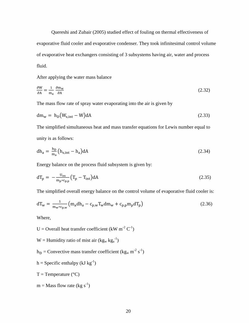
Quereshi and Zubair (2005) studied effect of fouling on thermal effectiveness of

evaporative fluid cooler and evaporative condenser. They took infinitesimal control volume

of evaporative heat exchangers consisting of 3 subsystems having air, water and process

fluid.

After applying the water mass balance

��m � @

*b �*&

�m (2.32)

The mass flow rate of spray water evaporating into the air is given by

dm0 � h�#WI,^_3 � W)dA (2.33)

The simplified simultaneous heat and mass transfer equations for Lewis number equal to

unity is as follows:

dhK � a�*b

#hI,^_3 � hK)dA (2.34)

Energy balance on the process fluid subsystem is given by:

dT� � � nc,*+�-+,+

#T� � T̂ _3)dA (2.35)

The simplified overall energy balance on the control volume of evaporative fluid cooler is:

dT0 � @*&�-+,&

#mKdhK � c�,0T0dm0 2 c�,�m�dT�) (2.36)

Where,

U = Overall heat transfer coefficient (kW m-2 C-1)

W = Humidity ratio of mist air (kgw kga-1)

h� = Convective mass transfer coefficient (kgw m-2 s-1)

h = Specific enthalpy (kJ kg-1)


m = Mass flow rate (kg s-1)

21

Subscripts

a = air

p = process fluid

w = water

int = air-water interface

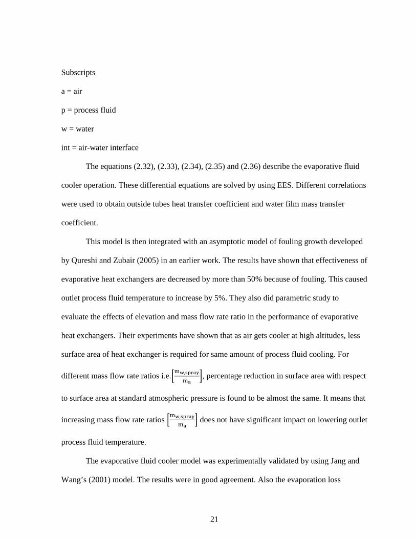
The equations (2.32), (2.33), (2.34), (2.35) and (2.36) describe the evaporative fluid

cooler operation. These differential equations are solved by using EES. Different correlations

were used to obtain outside tubes heat transfer coefficient and water film mass transfer

coefficient.

This model is then integrated with an asymptotic model of fouling growth developed

by Qureshi and Zubair (2005) in an earlier work. The results have shown that effectiveness of

evaporative heat exchangers are decreased by more than 50% because of fouling. This caused

outlet process fluid temperature to increase by 5%. They also did parametric study to

evaluate the effects of elevation and mass flow rate ratio in the performance of evaporative

heat exchangers. Their experiments have shown that as air gets cooler at high altitudes, less

surface area of heat exchanger is required for same amount of process fluid cooling. For

different mass flow rate ratios i.e.�*&,,+vb�*b

�, percentage reduction in surface area with respect

to surface area at standard atmospheric pressure is found to be almost the same. It means that

increasing mass flow rate ratios �*&,,+vb�*b

� does not have significant impact on lowering outlet

process fluid temperature.

The evaporative fluid cooler model was experimentally validated by using Jang and

Wang’s (2001) model. The results were in good agreement. Also the evaporation loss

22

errors were within -0.9 to 6 % when compared with the data provided by Baltimore Aircoil.

The value of h� is not known for most of the cases. Also the input parameters

required by the model are not readily available in manufacturer’s catalog data e.g. spray

water temperatures.

2.2 Dry fluid cooler models

Dry fluid coolers can be modeled using classic heat exchanger equations. There are 2

methods which are mainly reported in the literature to analyze heat exchangers.

1) Log mean temperature difference method

2) ℇ-NTU method

2.2.1 Log mean temperature difference (LMTD) method

The heat transfer of classic heat exchanger using LMTD method is given by

Q� � UA � LMTD (2.37)

Where,

LMTD � ∆%�(∆%t�_$∆%�/∆%t' (2.38)

For parallel heat exchangers

∆T@ � Ta,^_ � T-,^_

∆TM � Ta,\]3 � T-,\]3

For counter flow heat exchangers

∆T@ � Ta,^_ � T-,\]3

23

∆TM � Ta,\]3 � T-,^_

Subscripts

h = hot

c = cold

The main disadvantage of LMTD method is that it requires fluid temperatures as

inputs which are typically not known. If only the inlet fluid temperatures are known, a

cumbersome iterative procedure can be carried out to implement LMTD method. However,

in the same conditions ℇ-NTU method is much more convenient to use. Because of this

reason ℇ-NTU method is used to model fluid coolers in EnergyPlus.

2.2.2 ℇℇℇℇ-NTU method

Q� � ε � C� *^_ � $ta,^_ � t-,^_' (2.39)

Where,

C� *^_ � Min $C� a, C� -'

C� *K� � Max $C� a, C� -'

Cj � k� !fgk� !b�

= capacity ratio

Depending on heat exchanger configuration i.e. parallel flow, counter flow or cross

flow different correlations can be used to calculate � (effectiveness). For cross flow

configuration when both the streams are mixed, the ℇ-NTU correlation is given by

24

ε � 1 � exp �N$pqrsuv�'kv � (2.40)

Where,

NTU � UA/C� *^_ (2.41)

η � NTU(8.MM (2.42)

Eq. (2.40) is used in EnergyPlus to calculate effectiveness of dry fluid cooler.

In conclusion different fluid cooler models are studied. Their accuracy, range of

applicability and relative simplicity are discussed. Lebrun model is used with some

modification for the development of EnergyPlus’ evaporative fluid cooler model. Dry fluid

cooler is modeled as a classical heat exchanger by using ℇ-NTU correlations from cross flow

heat exchanger with both streams unmixed. Chapter 3 elaborates further the fluid cooler

models implemented in EnergyPlus.

25

CHAPTER III

DEVELOPMENT OF FLUIDCOOLER MODELS FOR ENERGYPLUS

In this chapter two new fluid cooler models were developed for EnergyPlus. The

chapter also discusses the catalog data provided by the fluid cooler manufacturers. Design

input parameters required by the model are presented and finally the actual model algorithms

and input specifications are explained.

3.1 Overview of the Models

The fluid cooler models are characterized by a single parameter, the overall heat

transfer coefficient-area product, UA. Generally, this parameter is not available and needs to

be calculated by using experimental data or manufacturer’s catalog data. The catalog data

available for fluid coolers are mostly insufficient. Also the manufacturers provide data only

for one rating point. There are some standard test conditions which are set by Cooling

Technology Institute (CTI) for cooling towers. Standard test conditions are 3 GPM/ton

entering water at 35°C (95°F), leaving water at 29.44°C (85°F), entering air at 25.56°C

26

(78°F) wet-bulb temperature and 35°C (95°F) dry-bulb temperature. The nominal capacity of

the cooling tower is the capacity specified at these conditions. Some evaporative fluid cooler

manufacturers provide catalog data on these standard test conditions. But a vast majority of

them don’t follow any standard conditions to publish catalog data. Because of the

insufficiency of catalog data, the UA values of the fluid coolers are determined for one rating

point only. Fig (3.1) shows the catalog data for evaporative fluid cooler taken from Baltimore

Aircoil’s website. In the figure, the capacity in U.S. Gallons per minute of water is shown.

The hot water/cold water temperatures are (95/85°F, 102/90°F and 115/90°F) and wet bulb

temperatures are (72°F, 78°F and 80°F).

Fig 3.1 Baltimore Aircoil’s catalog data for evaporative fluid coolers

27

Fig (3.2) shows the catalog data for Motivair Corp. dry fluid cooler. A single rating for

different fluid cooler model is shown in the figure.

Fig 3.2 Motivair corp. catalog data for dry fluid coolers

3.2 EnergyPlus model description

As discussed earlier, UA is single characterizing parameter for the fluid coolers. Two

input methods are mainly provided in EnergyPlus to specify fluid cooler performance which

are:

1) UA and design water flow rate

2) Design capacity method

28

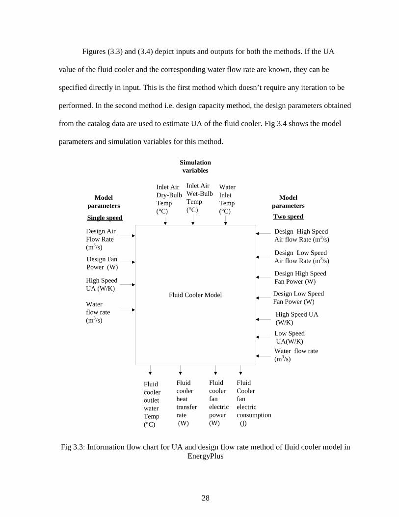
Figures (3.3) and (3.4) depict inputs and outputs for both the methods. If the UA

value of the fluid cooler and the corresponding water flow rate are known, they can be

specified directly in input. This is the first method which doesn’t require any iteration to be

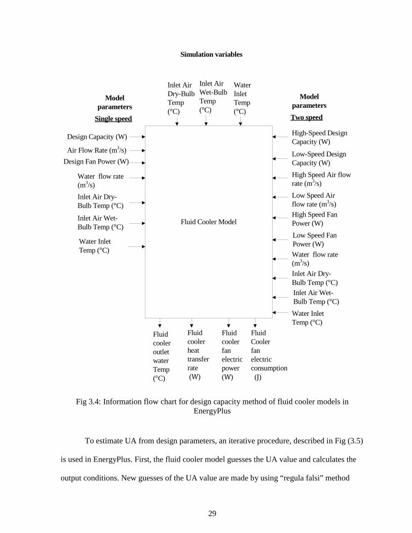
performed. In the second method i.e. design capacity method, the design parameters obtained

from the catalog data are used to estimate UA of the fluid cooler. Fig 3.4 shows the model

parameters and simulation variables for this method.

Fig 3.3: Information flow chart for UA and design flow rate method of fluid cooler model in EnergyPlus

Fluid Cooler Model

Design Air Flow Rate(m3/s)

Design Fan Power (W)

Single speed Two speed

Design High Speed Air flow Rate (m3/s)

Inlet Air Dry-Bulb Temp (°C)

Inlet Air Wet-Bulb Temp (°C)

Water Inlet Temp (°C)

Water flow rate(m3/s)

Fluid cooler heat transfer rate (W)

Fluid cooler fan electric power (W)

Fluid Coolerfan electric consumption (J)

Fluid cooler outlet water Temp (°C)

Design High Speed Fan Power (W)

Design Low Speed Fan Power (W)

High Speed UA (W/K)

Simulation variables


High Speed UA (W/K)

Design Low Speed Air flow Rate (m3/s)

Low Speed UA(W/K)

Model parameters

Model parameters

29

Fig 3.4: Information flow chart for design capacity method of fluid cooler models in EnergyPlus

To estimate UA from design parameters, an iterative procedure, described in Fig (3.5)

is used in EnergyPlus. First, the fluid cooler model guesses the UA value and calculates the

output conditions. New guesses of the UA value are made by using “regula falsi” method

Fluid Cooler Model

Air Flow Rate (m3/s)

Design Fan Power (W)

Single speed Two speed

High-Speed Design Capacity (W)

Low-Speed Design Capacity (W)

High Speed Air flow rate (m3/s)

Low Speed Air flow rate (m3/s)

Design Capacity (W)





Fluid cooler heat transfer rate (W)

Fluid cooler fan electric power (W)

Fluid Coolerfan electric consumption (J)

Fluid cooler outlet water Temp (°C)

High Speed Fan Power (W)

Low Speed Fan Power (W)

Inlet Air Dry-Bulb Temp (°C)Inlet Air Wet-Bulb Temp (°C)





Simulation variables

Model parameters

Model parameters


30

until the iteration converges to a unique solution. Once the UA value is determined, it is used

in the subsequent simulation calculations.

Fig 3.5 Flow chart for UA calculation method used by EnergyPlus

3.3 Implementing the Fluid Cooler Models in EnergyPlus

Since EnergyPlus is a modular simulation program, the dry and evaporative fluid

cooler models are implemented as two new modules in EnergyPlus. ℇ-NTU equations

described in section 2.2.2 are used to model dry fluid cooler and Lebrun model (section

2.1.2) is used as the basis to develop evaporative fluid cooler model in EnergyPlus. In the

Input data : tw,su, tdb,su twb,su, Qcatalogue, Va, Vw

Guess UA

Calculate fluid cooler outlet water temp.

Calculate fluid cooler capacity Qcalc

ABS (Qcatalogue -Qcalc) <error

Output: UA

No

Yes

New estimation of UA using Regula falsi

31

following sections, input specifications and actual algorithms of fluid cooler models

implemented in EnergyPlus are discussed.

3.3.1 Input specifications of fluid coolers

Inputs are specified in EnergyPlus by means of text files. These text files are called

IDD (input data dictionary) and IDF (input data file). Different object types and their

associated data are described in the IDD while the IDF contains all the input data needed for

simulation. The type of the object could be either numeric or alpha. The order of the data in

IDF must match the order of data in IDD i.e. each data value in the IDF must go hand in hand

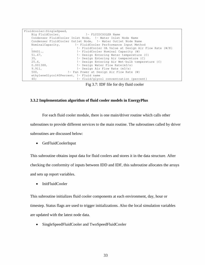
with IDD object. Fig (3.6) and (3.7) below show the IDD and IDF examples of dry fluid

cooler.

Fluidcooler:SingleSpeed, A1 , \field Name \required-field \type alpha \note fluidcooler name A2 , \field Water Inlet Node Name \required-field \type alpha \note Name of fluidcooler water inlet node A3 , \field Water Outlet Node Name \required-field \type alpha \note Name of fluidcooler water outlet node A4 , \field Performance Input Method \type Choice \key UAandDesignWaterFlowRate \key NominalCapacity \default NominalCapacity \note User can define fluidcooler thermal performance by specifying \note the fluidcooler UA and the Design Air Flow Rate, or by specifying \note the fluidcooler nominal capacity N1 , \field U-factor Times Area Value at Design Air Flow Rate \type real \units W/K \minimum> 0.0 \maximum 2100000.0 \autosizable \note Leave field blank if fluidcooler Performance Input Method is \note NOMINAL CAPACITY

32

N2 , \field Nominal Capacity \type real \units W \minimum> 0.0 \note Nominal fluidcooler capacity N3 , \field Design Entering Water Temperature \type real \units C \minimum> 0.0 \ip-units F N4 , \field Design Entering Air Temperature \type real \units C \minimum> 0.0 \ip-units F N5 , \field Design Entering Air Wet-bulb Temperature \type real \units C \minimum> 0.0 \ip-units F N6 , \field Design Water Flow Rate \type real \units m3/s \minimum> 0.0 \autosizable \ip-units gal/min N7 , \field Design Air Flow Rate \required-field \type real \units m3/s \minimum> 0.0 \autosizable N8 , \field Fan Power at Design Air Flow Rate \required-field \type real \units W \minimum> 0.0 \autosizable \ip-units W A5, \field Fluid Name \note (water, ethylene glycol, etc.) \type object-list \object-list GlycolConcentrations \required-field \default water N9, \field Fluid Glycol Concentration \required-field \type real \units percent \minimum 0 \maximum 100 \note with the rewrite of fluid properties this parameter \note is no longer needed A6 ; \field Outdoor Air Inlet Node Name \type alpha \note Enter the name of an outdoor air node

Fig 3.6: IDD file for dry fluid cooler

33

Fluidcooler:SingleSpeed, Big FluidCooler, !- FLUIDCOOLER Name Condenser FluidCooler Inlet Node, !- Water Inlet Node Name Condenser FluidCooler Outlet Node, !- Water Outlet Node Name NominalCapacity, !- FluidCooler Performance Input Method , !- FluidCooler UA Value at Design Air Flow Rate {W/K} 58601., !- FluidCooler Nominal Capacity {W} 51.67, !- Design Entering Water tempereture {C} 35, !- Design Entering Air tempereture {C} 25.6, !- Design Entering Air Wet-bulb tempereture {C} 0.001388, !- Design Water Flow Rate{m3/s} 9.911, !- Design Air Flow Rate {m3/s} 500, !- Fan Power at Design Air Flow Rate {W} ethyleneGlycol40Percent, !- Fluid name 40; !- fluid/glycol concentration {percent}

Fig 3.7: IDF file for dry fluid cooler

3.3.2 Implementation algorithm of fluid cooler models in EnergyPlus

For each fluid cooler module, there is one main/driver routine which calls other

subroutines to provide different services to the main routine. The subroutines called by driver

subroutines are discussed below:

• GetFluidCoolerInput

This subroutine obtains input data for fluid coolers and stores it in the data structure. After

checking the conformity of inputs between IDD and IDF, this subroutine allocates the arrays

and sets up report variables.

• InitFluidCooler

This subroutine initializes fluid cooler components at each environment, day, hour or

timestep. Status flags are used to trigger initializations. Also the local simulation variables

are updated with the latest node data.

• SingleSpeedFluidCooler and TwoSpeedFluidCooler

34

These subroutines simulate the operation of single and two speed fluid coolers respectively.

The subroutine calculates the period of time required to meet a leaving water temperature set-

point. It assumes that part-load operation represents a linear interpolation of two steady-state

regimes i.e. fluid cooler ON and OFF. The period of time required to meet the leaving water

temperature set-point is used to determine the required fan power and energy.

A RunFlag is passed by the upper level manager to indicate the ON/OFF status, or schedule,

of the fluid cooler. If the fluid cooler is OFF, outlet water temperature and flow rate are

passed through the model from inlet node to outlet node without intervention. Reports are

also updated with fan power and energy being zero.

When the RunFlag indicates an ON condition for the fluid cooler, the mass flow rate and

water temperature are read from the inlet node of the fluid cooler (water-side). The outdoor

air dry-bulb and wet-bulb temperatures are used as the air-side entering conditions to the dry

and evaporative fluid coolers respectively. The fluid cooler

fan is turned on and design parameters are used to calculate the leaving water temperature. If

the calculated leaving water temperature is below the set-point, a fan run-time fraction is

calculated and used to determine fan power. The fraction of time that the fluid cooler fans

must operate is calculated as follows:

ω � %,}e(%&cde,c==%&cde,cg(%&cde,c==

(3.1)

Where,

ω = Fan run time fraction


Subscripts

35

w = water

out = outlet condition

off = Fluid cooler fan OFF

on = Fluid cooler fan ON

set = set-point

The average fan power is calculated by multiplying ω by the steady-state fan power specified

as input. The leaving water temperature set-point is placed on the outlet node.

In the case of two speed fluid coolers, leaving water temperatures are calculated for low

speed operation. If the calculated leaving water temperature is at or above the set-point, the

fluid cooler fan is turned on 'high speed' and the routine is repeated. If the calculated leaving

water temperature is below the set-point, a fan run-time fraction is calculated for the second

stage fan and then the fan power is calculated. Eq. (3.2) shows the method of calculating fan

run time fraction.

ω � %,}e(%&cde,�c&%&cde,¤f¥¤(%&cde,�c&

(3.2)

The subscripts low and high stand for low speed and high speed fan operation respectively.

The average fan power for the simulation time step is calculated for the two-speed fluid

cooler as follows

Pfan,avg=ω(Pfan,high)+(1- ω) (Pfan,low) (3.3)

Where,

Pfan = Fan power (W)

If the calculated leaving water temperature is above the leaving water temperature set-point,

the calculated leaving water temperature is placed on the outlet node and the fan runs at full

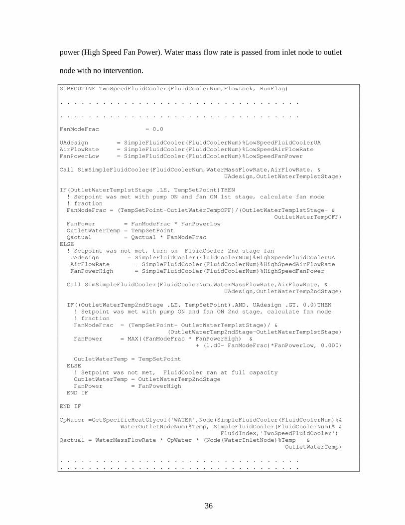
36

power (High Speed Fan Power). Water mass flow rate is passed from inlet node to outlet

node with no intervention.

SUBROUTINE TwoSpeedFluidCooler(FluidCoolerNum,FlowLock, RunFlag) . . . . . . . . . . . . . . . . . . . . . . . . . . . . . . . . . . . . . . . . . . . . . . . . . . . . . . . . . . . . . . . . . . . . FanModeFrac = 0.0 UAdesign = SimpleFluidCooler(FluidCoolerNum)%LowSpeedFluidCoolerUA AirFlowRate = SimpleFluidCooler(FluidCoolerNum)%LowSpeedAirFlowRate FanPowerLow = SimpleFluidCooler(FluidCoolerNum)%LowSpeedFanPower Call SimSimpleFluidCooler(FluidCoolerNum,WaterMassFlowRate,AirFlowRate, & UAdesign,OutletWaterTemp1stStage) IF(OutletWaterTemp1stStage .LE. TempSetPoint)THEN ! Setpoint was met with pump ON and fan ON 1st stage, calculate fan mode ! fraction FanModeFrac = (TempSetPoint-OutletWaterTempOFF)/(OutletWaterTemp1stStage- & OutletWaterTempOFF) FanPower = FanModeFrac * FanPowerLow OutletWaterTemp = TempSetPoint Qactual = Qactual * FanModeFrac ELSE ! Setpoint was not met, turn on FluidCooler 2nd stage fan UAdesign = SimpleFluidCooler(FluidCoolerNum)%HighSpeedFluidCoolerUA AirFlowRate = SimpleFluidCooler(FluidCoolerNum)%HighSpeedAirFlowRate FanPowerHigh = SimpleFluidCooler(FluidCoolerNum)%HighSpeedFanPower Call SimSimpleFluidCooler(FluidCoolerNum,WaterMassFlowRate,AirFlowRate, & UAdesign,OutletWaterTemp2ndStage) IF((OutletWaterTemp2ndStage .LE. TempSetPoint).AND. UAdesign .GT. 0.0)THEN ! Setpoint was met with pump ON and fan ON 2nd stage, calculate fan mode ! fraction FanModeFrac = (TempSetPoint- OutletWaterTemp1stStage)/ & (OutletWaterTemp2ndStage-OutletWaterTemp1stStage) FanPower = MAX((FanModeFrac * FanPowerHigh) & + (1.d0- FanModeFrac)*FanPowerLow, 0.0D0) OutletWaterTemp = TempSetPoint ELSE ! Setpoint was not met, FluidCooler ran at full capacity OutletWaterTemp = OutletWaterTemp2ndStage FanPower = FanPowerHigh END IF END IF CpWater =GetSpecificHeatGlycol('WATER',Node(SimpleFluidCooler(FluidCoolerNum)%& WaterOutletNodeNum)%Temp, SimpleFluidCooler(FluidCoolerNum)% & FluidIndex,'TwoSpeedFluidCooler') Qactual = WaterMassFlowRate * CpWater * (Node(WaterInletNode)%Temp – & OutletWaterTemp) . . . . . . . . . . . . . . . . . . . . . . . . . . . . . . . . . . . . . . . . . . . . . . . . . . . . . . . . . . . . . . . . . . . .

37

RETURN END SUBROUTINE TwoSpeedFluidCooler

This subroutine calls SimSimpleFluidCooler and SimSimpleEvapFluidCooler subroutines in

dry and evaporative fluid cooler modules respectively to calculate outlet water temperature

and heat transfer rate from fluid coolers. The subroutines for dry and evaporative fluid

coolers are described below:

SUBROUTINE SimSimpleFluidCooler(FluidCoolerNum,WaterMassFlowRate,& AirFlowRate,UAdesign,OutletWaterTemp) . . . . . . . . . . . . . . . . . . . . . . . . . . . . . . . . . . . . . . . . . . . . . . . . . . . . . . . . . . . . . . . . . . . . MdotCpWater = WaterMassFlowRate * CpWater AirCapacity = AirMassFlowRate * CpAir ! calculate the minimum to maximum capacity ratios of airside and waterside CapacityRatioMin = MIN(AirCapacity,MdotCpWater) CapacityRatioMax = MAX(AirCapacity,MdotCpWater) CapacityRatio = CapacityRatioMin/CapacityRatioMax ! Calculate heat transfer coefficient and number of transfer units (NTU) NumTransferUnits = UAdesign/CapacityRatioMin ETA=NumTransferUnits**0.22d0 A=CapacityRatio*NumTransferUnits/ETA effectiveness = 1.d0 - Exp((Exp(-A) - 1.d0) / (CapacityRatio / ETA)) ! calculate water to air heat transfer Qactual = effectiveness * CapacityRatioMin * (InletWaterTemp-InletAirTemp) ! calculate new exiting dry bulb temperature of airstream OutletAirTemp = InletAirTemp + Qactual/AirCapacity IF(Qactual .GE. 0.0)THEN OutletWaterTemp = InletWaterTemp - Qactual/ MdotCpWater ELSE OutletWaterTemp = InletWaterTemp END IF RETURN END SUBROUTINE SimSimpleFluidCooler

SUBROUTINE SimSimpleEvapFluidCooler(EvapFluidCoolerNum, WaterMassFlowRate, AirFlowRate,UAdesign,OutletWaterTemp) INTEGER, PARAMETER :: IterMax = 50 ! Maximum number of iterations allowed REAL(r64), PARAMETER :: WetBulbTolerance = 0.00001d0 ! Maximum error for exiting wet-bulb temperature between iterations [delta K/K] REAL(r64), PARAMETER :: DeltaTwbTolerance = 0.001d0 ! Maximum error (tolerance) in DeltaTwb for iteration convergence [C] . . . . . . . . . . . . . . . . . . . . . . . . . . . . . . . . . .

38

. . . . . . . . . . . . . . . . . . . . . . . . . . . . . . . . . . ! initialize exiting wet bulb temperature before iterating on final solution OutletAirWetBulb = InletAirWetBulb + 6.0 ! Calcluate mass flow rates MdotCpWater = WaterMassFlowRate * CpWater Iter = 0 DO WHILE ((WetBulbError.GT.WetBulbTolerance) .AND. (Iter.LE.IterMax) .AND. & (DeltaTwb.GT.DeltaTwbTolerance)) Iter = Iter + 1 OutletAirEnthalpy = PsyHFnTdbRhPb(OutletAirWetBulb,1.0d0, & SimpleEvapFluidCoolerInlet(EvapFluidCoolerNum)%AirPress) ! calculate the airside specific heat and capacity CpAirside = (OutletAirEnthalpy - InletAirEnthalpy)/(OutletAirWetBulb- & InletAirWetBulb) AirCapacity = AirMassFlowRate * CpAirside ! calculate the minimum to maximum capacity ratios of airside and waterside CapacityRatioMin = MIN(AirCapacity,MdotCpWater) CapacityRatioMax = MAX(AirCapacity,MdotCpWater) CapacityRatio = CapacityRatioMin/CapacityRatioMax ! Calculate heat transfer coefficient and number of transfer units (NTU) UAactual = UAdesign*CpAirside/CpAir NumTransferUnits = UAactual/CapacityRatioMin ! calculate heat exchanger effectiveness IF (CapacityRatio.LE.0.995d0)THEN effectiveness = (1.d0-EXP(-1.0d0*NumTransferUnits*(1.0d0-CapacityRatio)))/& (1.0d0-CapacityRatio*EXP(-1.0d0*NumTransferUnits*(1.0d0-CapacityRatio))) ELSE effectiveness = NumTransferUnits/(1.d0+NumTransferUnits) ENDIF ! calculate water to air heat transfer and store last exiting WB temp of air Qactual = effectiveness * CapacityRatioMin * (InletWaterTemp-InletAirWetBulb) OutletAirWetBulbLast = OutletAirWetBulb ! calculate new exiting wet bulb temperature of airstream OutletAirWetBulb = InletAirWetBulb + Qactual/AirCapacity ! Check error tolerance and exit if satisfied DeltaTwb = ABS(OutletAirWetBulb - InletAirWetBulb) ! Add KelvinConv to denominator below convert OutletAirWetBulbLast to Kelvin ! to avoid divide by zero. ! Wet bulb error units are delta K/K WetBulbError = ABS((OutletAirWetBulb - OutletAirWetBulbLast)/ & (OutletAirWetBulbLast+KelvinConv)) END DO IF(Qactual .GE. 0.0)THEN OutletWaterTemp = InletWaterTemp - Qactual/ MdotCpWater ELSE OutletWaterTemp = InletWaterTemp END IF RETURN END SUBROUTINE SimSimpleEvapFluidCooler

39

• SizeFluidCooler

The fluid cooler UA value is calculated in this subroutine. The method used to calculate UA

is described in Fig (3.3). First, the UA value is guessed on the basis of design capacity of the

fluid cooler and capacity of the fluid cooler which is based on this UA is calculated. If the

residual of the capacity is less than the specified accuracy then the desired UA value is

obtained. Otherwise new UA value is calculated by using regula falsi and iterations are

performed until the solution converges to a UA value for which residual is less than the

accuracy.

IF (SimpleFluidCooler(FluidCoolerNum)%PerformanceInputMethod == & 'NOMINALCAPACITY') THEN IF (SimpleFluidCooler(FluidCoolerNum)%DesignWaterFlowRate >= &

SmallWaterVolFlow) THEN DesFluidCoolerLoad = SimpleFluidCooler(FluidCoolerNum)% & FluidCoolerNominalCapacity Par(1) = DesFluidCoolerLoad Par(2) = REAL(FluidCoolerNum,r64) ! FluidCooler number Par(3) = GetDensityGlycol('WATER',InitConvTemp, & SimpleFluidCooler(FluidCoolerNum)%FluidIndex,CalledFrom) & * SimpleFluidCooler(FluidCoolerNum)%DesignWaterFlowRate ! design water mass flow rate Par(4) = SimpleFluidCooler(FluidCoolerNum)%HighSpeedAirFlowRate ! design air volume flow rate Par(5) = GetSpecificHeatGlycol('WATER',SimpleFluidCooler(FluidCoolerNum)% & DesignEnteringWaterTemp, SimpleFluidCooler(FluidCoolerNum)% & FluidIndex,CalledFrom) UA0 = 0.0001d0 * DesFluidCoolerLoad ! Assume deltaT = 10000K (limit) UA1 = DesFluidCoolerLoad ! Assume deltaT = 1K SimpleFluidCoolerInlet(FluidCoolerNum)%WaterTemp = & SimpleFluidCooler(FluidCoolerNum)%DesignEnteringWaterTemp ! design inlet water temperature SimpleFluidCoolerInlet(FluidCoolerNum)%AirTemp = & SimpleFluidCooler(FluidCoolerNum)%DesignEnteringAirTemp ! design inlet air dry-bulb temp SimpleFluidCoolerInlet(FluidCoolerNum)%AirWetBulb = & SimpleFluidCooler(FluidCoolerNum)%DesignEnteringAirWetbulbTemp ! design inlet air wet-bulb temp SimpleFluidCoolerInlet(FluidCoolerNum)%AirPress = StdBaroPress SimpleFluidCoolerInlet(FluidCoolerNum)%AirHumRat = & PsyWFnTdbTwbPb(SimpleFluidCoolerInlet(FluidCoolerNum)%AirTemp, & SimpleFluidCoolerInlet(FluidCoolerNum)%AirWetBulb, & SimpleFluidCoolerInlet(FluidCoolerNum)%AirPress) CALL SolveRegulaFalsi(Acc, MaxIte, SolFla, UA, &

40

SimpleFluidCoolerUAResidual,UA0, UA1, Par) IF (SolFla == -1) THEN CALL ShowSevereError('Iteration limit exceeded in calculating & FluidCooler UA') CALL ShowFatalError('Autosizing of FluidCooler UA failed for & FluidCooler '//TRIM(SimpleFluidCooler(FluidCoolerNum)%Name)) ELSE IF (SolFla == -2) THEN CALL ShowSevereError('Bad starting values for UA') CALL ShowFatalError('Autosizing of FluidCooler UA failed for & FluidCooler '//TRIM(SimpleFluidCooler(FluidCoolerNum)%Name)) ENDIF SimpleFluidCooler(FluidCoolerNum)%HighSpeedFluidCoolerUA = UA ELSE SimpleFluidCooler(FluidCoolerNum)%HighSpeedFluidCoolerUA = 0.0 ENDIF . . . . . . . . . . . . . . . . . . . . . . . . . . . . . . . . . . . . . . . . . . . . . . . . . . . . . . . . . . . . . . . . . . . . ENDIF

FUNCTION SimpleFluidCoolerUAResidual(UA, Par) RESULT (Residuum) . . . . . . . . . . . . . . . . . . . . . . . . . . . . . . . . . . . . . . . . . . . . . . . . . . . . . . . . . . . . . . . . . . . . ! SUBROUTINE ARGUMENT DEFINITIONS: REAL(r64), INTENT(IN) :: UA ! UA of FluidCooler REAL(r64), INTENT(IN), DIMENSION(:), OPTIONAL :: Par ! par(1) = design FluidCooler load [W] ! par(2) = FluidCooler number ! par(3) = design water mass flow rate [kg/s] ! par(4) = design air volume flow rate [m3/s] ! par(5) = water specific heat [J/(kg*C)] REAL(r64) :: Residuum ! residual to be minimized to zero ! FUNCTION LOCAL VARIABLE DECLARATIONS: INTEGER :: FluidCoolerIndex ! index of this FluidCooler REAL(r64) :: OutWaterTemp ! outlet water temperature [C] REAL(r64) :: Output ! FluidCooler output [W] FluidCoolerIndex = INT(Par(2)) CALL SimSimpleFluidCooler(FluidCoolerIndex,Par(3),Par(4),UA,OutWaterTemp) Output = Par(5)*Par(3)*(SimpleFluidCoolerInlet(FluidCoolerIndex)%WaterTemp – & OutWaterTemp) Residuum = (Par(1) - Output) / Par(1) RETURN END FUNCTION SimpleFluidCoolerUAResidual

• UpdateRecords

This subroutine is used to pass the results to outlet node. Outlet water temperature and water

mass flow rates are passed to the outlet node. This subroutine also issues warning in the case

41

of outlet water temperature being lower than the loop temperature, water mass flow rate

being greater than loop maximum flow rate or lower than loop minimum flow rate.

42

CHAPTER IV

PERFORMANCE EVALUATION OF ENERGYPLUS FLUID COOLER MODELS

One major problem which was encountered while modeling fluid coolers in

EnergyPlus was the insufficient catalog data. More often than not, manufacturers don’t

provide enough data. The absence of required design parameters creates problem for

modeling. The objective of this chapter is to evaluate the impact of various design parameters

in the results of simulation. This will help to recognize the parameters which are really

important from simulation point of view. The parameters for which model is very sensitive

must be input with least errors while the parameters for which model is very less sensitive

can be guessed by using engineering judgment. As discussed in chapter in chapter 3, overall

heat transfer coefficient (UA) is the single characterizing parameter for the fluid cooler

models. So first the sensitivity of UA with respect to design parameters is discussed and then

the sensitivity of simulation result with respect to UA is considered.

43

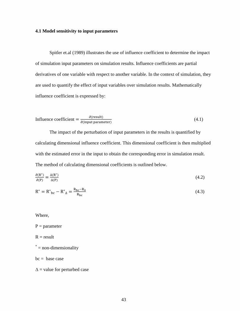
4.1 Model sensitivity to input parameters

Spitler et.al (1989) illustrates the use of influence coefficient to determine the impact

of simulation input parameters on simulation results. Influence coefficients are partial

derivatives of one variable with respect to another variable. In the context of simulation, they

are used to quantify the effect of input variables over simulation results. Mathematically

influence coefficient is expressed by:

Influence coefficient � �$jNI]�3'�$^_�]3 �KjK*N3Nj' (4.1)

The impact of the perturbation of input parameters in the results is quantified by

calculating dimensional influence coefficient. This dimensional coefficient is then multiplied

with the estimated error in the input to obtain the corresponding error in simulation result.

The method of calculating dimensional coefficients is outlined below.

�$w�'�$¦' � ∆$w�'

∆$¦' (4.2)

R� � R�`- � R�∆ � who(w∆who

(4.3)

Where,

P = parameter

R = result

* = non-dimensionality

bc = base case

∆ = value for perturbed case

44

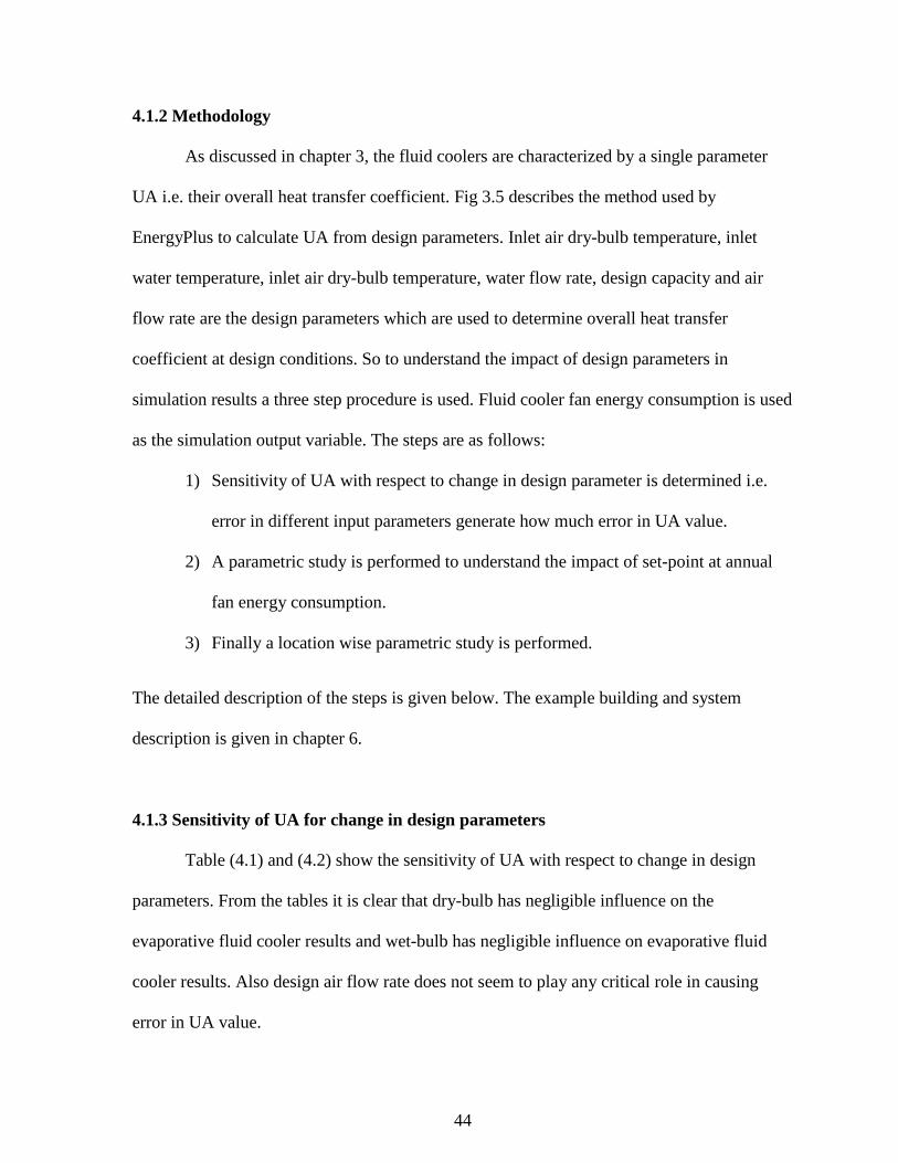
4.1.2 Methodology

As discussed in chapter 3, the fluid coolers are characterized by a single parameter

UA i.e. their overall heat transfer coefficient. Fig 3.5 describes the method used by

EnergyPlus to calculate UA from design parameters. Inlet air dry-bulb temperature, inlet

water temperature, inlet air dry-bulb temperature, water flow rate, design capacity and air

flow rate are the design parameters which are used to determine overall heat transfer

coefficient at design conditions. So to understand the impact of design parameters in

simulation results a three step procedure is used. Fluid cooler fan energy consumption is used

as the simulation output variable. The steps are as follows:

1) Sensitivity of UA with respect to change in design parameter is determined i.e.

error in different input parameters generate how much error in UA value.

2) A parametric study is performed to understand the impact of set-point at annual

fan energy consumption.

3) Finally a location wise parametric study is performed.

The detailed description of the steps is given below. The example building and system

description is given in chapter 6.

4.1.3 Sensitivity of UA for change in design parameters

Table (4.1) and (4.2) show the sensitivity of UA with respect to change in design

parameters. From the tables it is clear that dry-bulb has negligible influence on the

evaporative fluid cooler results and wet-bulb has negligible influence on evaporative fluid

cooler results. Also design air flow rate does not seem to play any critical role in causing

error in UA value.

45

Table 4.1 UA sensitivity for dry fluid cooler

Dry Fluid Cooler Design Parameter

Base –case Value

Dimensional I.C. Est. Error

(Parameter) Est. Error (Result)

Design Inlet air dry-bulb temp.

37.78°C 0.17881292 °C-1

5 °C ±89.4065%

Design Inlet air wet-bulb temp.

30°C 0.000259776 °C-1

5 °C ±0.129888%

Design Air flow rate

9.675(m3/s) 0.0673012 (m3/s)-1

2 m3/s ±0.0252 %

Design Water flow rate

4.10E-03 (m3/s)

11.176952 (m3/s)-1

0.001 m3/s ±1.1177%

Design Capacity 93753W 1.84109E-05 W-1 9375 W ±17.26019%

Design Inlet Water temp.

54.44 °C 0.084153265 °C-1 5 °C ±42.07663%

Table 4.2 UA sensitivity for evaporative fluid cooler

Evaporative Fluid Cooler Design Parameter

Base –case Value

Dimensional I.C. Est. Error

(Parameter) Est. Error (Result)

Design Inlet air dry-bulb temp.

35°C 0.000494709°C-1

5 °C ±0.247354%

Design Inlet air wet-bulb temp.

25.6°C 0.25002285 °C-1

5 °C ±125.011%

Design Air flow rate

7.164(m3/s) 0.0164129 (m3/s)-1

2 m3/s ±3.28258%

Design Water flow rate

3.98E-03 (m3/s)

125.17795 (m3/s)-1

0.001 m3/s ±12.5178%

Design Capacity 73854W 1.94928E-05 W-1 7385 ±14.39542%

Design Inlet Water temp.

35 °C

0.1109253 °C-1

5 °C ±55.46267%

46

4.2 Parametric study with different set-point temperatures

As discussed in chapter 3, set-point for the fluid cooler can either be a fixed set-point

temperature or the outdoor air dry/wet-bulb temperature depending upon the requirements for

a particular application. If no fixed value of the set-point is provided then outdoor dry-bulb

and wet-bulb temperatures can be used as the set-points for dry and evaporative fluid coolers

respectively. This section discusses the change in annual fan energy consumption of fluid

coolers at different set-point temperatures. Table 4.3 and 4.4 show the results of the study.

From the tables it is clear that annual fan energy consumption is more sensitive to UA value

at higher set-point temperatures.

Table 4.3 Change in dry fluid cooler fan energy consumption at different set-points

Dry Fluid Cooler

Set-Point

Annual fan energy consumption (J) % change in results (UA=10674 W/K) (UA=9674 W/K)

95°F (35 °C)

3.60E+08 3.78E+08 -5.14673 %

90°F (32.22 °C)

4.75E+08 4.95E+08 -4.20965 %

85°F (29.44 °C)

6.09E+08 6.27E+08 -2.99141 %

80°F (26.67 °C)

7.44E+08 7.61E+08 -2.2531 %

75°F (23.89 °C)

8.70E+08 8.82E+08 -1.36968 %

70°F (21.11°C)

9.59E+08 9.67E+08 -0.80211 %

Out dry-bulb

3.78E+08 3.78E+08 0

47

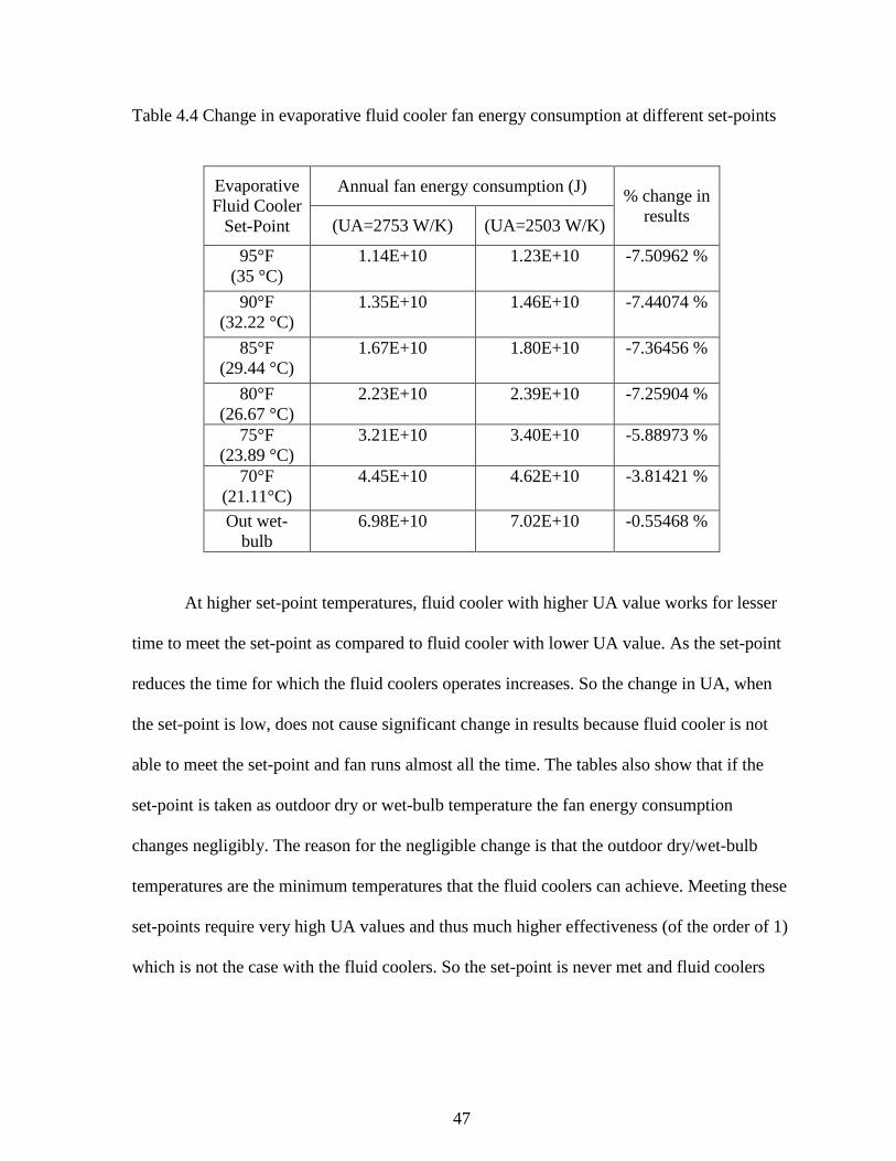
Table 4.4 Change in evaporative fluid cooler fan energy consumption at different set-points

Evaporative Fluid Cooler

Set-Point

Annual fan energy consumption (J) % change in results (UA=2753 W/K) (UA=2503 W/K)

95°F (35 °C)

1.14E+10 1.23E+10 -7.50962 %

90°F (32.22 °C)

1.35E+10 1.46E+10 -7.44074 %

85°F (29.44 °C)

1.67E+10 1.80E+10 -7.36456 %

80°F (26.67 °C)

2.23E+10 2.39E+10 -7.25904 %

75°F (23.89 °C)

3.21E+10 3.40E+10 -5.88973 %

70°F (21.11°C)

4.45E+10 4.62E+10 -3.81421 %

Out wet-bulb

6.98E+10

7.02E+10

-0.55468 %

At higher set-point temperatures, fluid cooler with higher UA value works for lesser

time to meet the set-point as compared to fluid cooler with lower UA value. As the set-point

reduces the time for which the fluid coolers operates increases. So the change in UA, when

the set-point is low, does not cause significant change in results because fluid cooler is not

able to meet the set-point and fan runs almost all the time. The tables also show that if the

set-point is taken as outdoor dry or wet-bulb temperature the fan energy consumption

changes negligibly. The reason for the negligible change is that the outdoor dry/wet-bulb

temperatures are the minimum temperatures that the fluid coolers can achieve. Meeting these

set-points require very high UA values and thus much higher effectiveness (of the order of 1)

which is not the case with the fluid coolers. So the set-point is never met and fluid coolers

48

keep running all the time. For this case, even changing the UA value by a large amount does

not cause any significant change in the output as the set-point is still not met.

4.3 Parametric study at different locations

It is clear from tables (4.3) and (4.4), that the fan energy consumption is more

sensitive to UA value at higher set-point temperatures. The study of section 4.2 is extended

to cover for different locations. Five different locations in USA are chosen and annual fan

energy consumption was calculated at each location. The UA values of the fluid coolers are

same as shown in tables (4.3) and (4.4). The simulations were carried out for two different

set-point temperatures 85°F (29.44°C) and outdoor dry-bulb (for dry fluid cooler) or wet-bulb

(for evaporative fluid cooler) temperatures. Fig (4.1) and (4.2) show the results of the

parametric study. The figures substantiate the previously drawn conclusion that when the set-

point is outdoor dry or wet-bulb temperatures, the change in UA causes negligible change in

annual fan energy consumption because the fluid cooler is not able to meet the set-point for

both the UA values. So it runs all the time for both UA values. For a fixed set-point, the

percentage change in fan energy consumption for different locations is shown below.

49

Fig 4.1 Comparison of % change in dry fluid cooler fan energy consumption due to change in

UA value at different locations for two different set-points

Fig 4.2 Comparison of % change in evaporative fluid cooler fan energy consumption due to

change in UA value at different locations for two different set-points

0

1

2

3

4

5

6

1 2 3 4 5

% C

ha

ng

e i

n a

nn

ua

l fa

n e

ne

rgy

co

nsu

mp

tio

n

Locations

Out dry-bulb

85 F set-point

Seattle MiamiPhoenixSanfransisco Chicago

0

1

2

3

4

5

6

7

8

9

1 2 3 4 5

% C

ha

ng

e i

n a

nn

ua

l fa

n e

ne

rgy

co

nsu

mp

tio

n

Locations

85 F set-point

Out Wet-bulb

Seattle MiamiPhoenixSanfransisco Chicago

50

4.4 Summary of results

The model sensitivity analysis can be summarized as follows:

1) In the absence of sufficient manufacturer’s data, dry-bulb temperature for evaporative

fluid cooler and wet-bulb temperature for dry fluid cooler can be guessed with

negligible error in the simulation results.

2) If the set-point temperature is chosen as dry or wet-bulb temperature for dry and

evaporative fluid cooler respectively, then it is possible that significant change in UA

value will cause negligible change in the simulation results. The reason for this

behavior is that the fluid cooler UA value has to be very large (effectiveness equal to

one) to reach to the set-point. If the fluid cooler UA value is not that high it will not

meet the set-point. In this case, if the UA value of the fluid cooler will be changed it

will still not meet the set-point. So the fan which was running at full speed will

continue to do so and fan energy consumption will remain unchanged.

3) Change in UA value causes more difference in the simulation results at higher set-

point temperatures than at lower set-points. In other words, if the set-point for the

fluid cooler is increased, the magnitude of difference in simulation results for the

same change in UA will increase.

4) Inlet air wet-bulb temperature, design air flow rate and design water flow rate have

very less impact on the fan energy consumption in the case of dry fluid coolers. While

in the case of evaporative fluid coolers, inlet air dry-bulb temperature and design air

flow rate have negligible effect over the fan energy consumption.

51

5) Fluid cooler UA value must be carefully chosen when the set-point temperature is

defined by the users. Because as the set-point temperature increases, the simulation

results become more sensitive to UA.

52

CHAPTER V

MODEL VERIFICATION

The published catalog data for fluid coolers are mostly insufficient. Moreover, the

data is available only for one rating point for a particular fluid cooler model. Very few fluid

cooler manufacturers provide the data for part load conditions. Some times, design input

parameters e.g. inlet air dry-bulb temperatures, inlet air wet-bulb temperature, air flow rate

etc. are missing. In this chapter, evaporative fluid cooler models are verified by using

Baltimore Aircoil’s catalog data. The data is obtained from their website for multiple rating

points. For dry fluid coolers, because of lack of catalog data, the model is verified by using

HVACSIM+ dry fluid cooler model (Type 762). Evaporative fluid cooler model is also

verified by using Lebrun model, discussed earlier in chapter 2, which is implemented in

VBA.

5.1 Evaporative fluid cooler: Comparison with published data sets

Data for evaporative fluid coolers is much more extensively and readily available as

compare to dry fluid coolers. Evaporative fluid cooler’s data is taken from Baltimore Aircoil

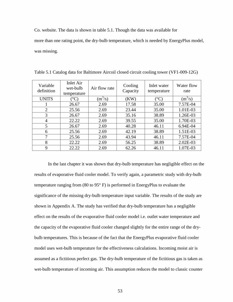
53

Co. website. The data is shown in table 5.1. Though the data was available for

more than one rating point, the dry-bulb temperature, which is needed by EnergyPlus model,

was missing.

Table 5.1 Catalog data for Baltimore Aircoil closed circuit cooling tower (VF1-009-12G)

Variable definition

Inlet Air wet-bulb

temperature Air flow rate

Cooling Capacity

Inlet water temperature

Water flow rate

UNITS (°C) (m3/s) (KW) (°C) (m3/s) 1 26.67 2.69 17.58 35.00 7.57E-04 2 25.56 2.69 23.44 35.00 1.01E-03 3 26.67 2.69 35.16 38.89 1.26E-03 4 22.22 2.69 39.55 35.00 1.70E-03 5 26.67 2.69 40.28 46.11 6.94E-04 6 25.56 2.69 42.19 38.89 1.51E-03 7 25.56 2.69 43.94 46.11 7.57E-04 8 22.22 2.69 56.25 38.89 2.02E-03 9 22.22 2.69 62.26 46.11 1.07E-03

In the last chapter it was shown that dry-bulb temperature has negligible effect on the

results of evaporative fluid cooler model. To verify again, a parametric study with dry-bulb

temperature ranging from (80 to 95° F) is performed in EnergyPlus to evaluate the

significance of the missing dry-bulb temperature input variable. The results of the study are

shown in Appendix A. The study has verified that dry-bulb temperature has a negligible

effect on the results of the evaporative fluid cooler model i.e. outlet water temperature and

the capacity of the evaporative fluid cooler changed slightly for the entire range of the dry-

bulb temperatures. This is because of the fact that the EnergyPlus evaporative fluid cooler

model uses wet-bulb temperature for the effectiveness calculations. Incoming moist air is

assumed as a fictitious perfect gas. The dry-bulb temperature of the fictitious gas is taken as

wet-bulb temperature of incoming air. This assumption reduces the model to classic counter

54

flow heat exchanger and the effectiveness of the heat exchanger is then calculated. The dry-

bulb temperature is used only to calculate specific heat and density of air which don’t vary

too much in the dry-bulb range stated above. Since there was negligible difference in the

output as a result of changing dry-bulb temperature, 90° F dry-bulb temperature is chosen to

make up for the missing dry-bulb data. Each individual rating point is used as input one by

one, corresponding UA value is calculated by EnergyPlus and then simulations are

performed. The capacity obtained from the model is compared with the published capacity.

As fig. 5.1 shows, the error between the cooling capacities published by manufacturer and

calculated from EnergyPlus is less than 0.025 %.

Fig. 5.1 Catalogue data Vs EnergyPlus capacity (KW)

0

10

20

30

40

50

60

70

0 15 30 45 60 75

En

erg

yP

lus

Ca

pa

city

(K

W)

Capacity catalogue data (KW)

EnergyPlus Vs. Catalog

Capacity

0 % error line

5%

-5%

55

5.2 Dry fluid cooler: Comparison between EnergyPlus and HVACSIM+ models

Xiaowei Xu (2007) developed dry fluid cooler model (Type 762) for HVACSIM+.

Both HVACSIM+ and EnergyPlus dry fluid cooler models use classic heat exchanger (ℇ-

NTU) equation to calculate effectiveness of the heat exchanger. Input requirements of both

the models are same with the main difference that EnergyPlus model can calculate UA value

if not given by the user while HVACSIM+ model essentially needs UA value as input

parameter.

For comparison, first EnergyPlus simulation is run for a design day (21 July) using

weather data of Chicago. The description of the building and the system are given in detail in

chapter 6. Dry fluid cooler’s outlet water temperature and capacity are obtained as a result of

simulation. Then HVACSIM+ dry fluid model (Type 762) is simulated for the same input

conditions which are used for EnergyPlus simulation. The boundary file of HVACSIM+ dry

fluid cooler model had the same inlet air and water mass flow rates and same inlet air and

water temperatures as in the EnergyPlus inputs. The UA value of the fluid cooler calculated

by EnergyPlus is taken as input parameter to HVACSIM+. The simulations were performed

and the results were compared. The error between the results was initially high. It was found

that there were bugs in the source code of dry fluid cooler model of HVACSIM+. The heat

transfer equation and the outlet water temperature calculation equations were based on

specific heat (Cp) of the both the fluids while they should be based on capacity flow rates

(M*Cp) of the fluids. The erroneous lines of the code are shown below:

Present code (Incorrect)

Twex=Twsu-cpMoistAir*(Tdbex-Tdbsu)/C_fluid

56

Q=C_fluid*(Twsu-Twex)

Correct code

Twex=Twsu-CrAir*(Tdbex-Tdbsu)/CrW

Q=CrW*(Twsu-Twex)

The internal variables are defined as follows:

cpMoistAir: Moist air specific heat (J/kg/K)

C_fluid: Fluid specific heat (J/kg/K)

CrW: Water heat capacity flow rate (W/K)

CrAir: Air heat capacity flow rate (W/K)

The bugs were fixed but still the results were 3-4% off. Then some intermediate

variables are set to investigate the problem further and figure out the cause of this difference.

It was found that specific heat capacity (Cp) calculated by HVACSIM+ is not in agreement

with specific heat capacity (Cp) calculated by EnergyPlus. For example, the Cp of the water

calculated by HVACSIM+ for 39.2°C and 24.5°C entering water temperature was found to

be 3444.43 (J/kg-K) and 3617 (J/kg-K) respectively while the values obtained from the

EnergyPlus calculations and tables are approximately 4180 (J/kg-K) for both the cases. The

correct Cp value (i.e. 4180 (J/kg-K)) is hardwired in HVACSIM+ model and simulation was

run again. Table 5.2 shows the input parameters and simulation variables used by both the

models. The process fluid is water. As shown in Fig 5.2 the error between the capacities

calculated by HVACSIM+ and EnergyPlus is less than 0.3 % error for a very large range of

input conditions.

57

Table 5.2 Input parameters and simulation outputs of HVACSIM+ and EnergyPlus dry fluid

cooler models

EnergyPlus HVACSIM+

Inlet Air

Temp (°C)

Inlet Water Temp (°C)

Water Mass Flow rate

(m3/s)

Air Mass Flow rate

(m3/s)

UA (W/K)

Q (W)

Outlet Water Temp (°C)

Q (W)

Outlet Water Temp (°C)

21.71 30.78 1.39 11.34 7233.24 32117.3 25.24 32078 25.25 21.71 28.76 1.39 11.34 7233.24 24975.4 24.46 24934.2 24.46 21.71 26.71 1.39 11.34 7233.24 17692.1 23.66 17649 23.66 21.71 26.05 1.39 11.34 7233.24 15377.8 23.40 15361.9 23.4 21.87 24.52 1.39 11.33 7233.24 9366.3 22.90 9356.8 22.9 21.87 25.15 1.39 11.33 7233.24 11600.2 23.15 11588.1 23.15 22.98 27.35 1.39 11.29 7233.24 15460.3 24.68 15443.7 24.7 23.21 27.49 1.39 11.28 7233.24 15165.6 24.88 15194.8 24.88 24.44 28.66 1.39 11.23 7233.24 14939.8 26.09 14901.4 26.1 25.24 29.05 1.39 11.20 7233.24 13476.5 26.73 13447.8 26.75 26.11 29.98 1.39 11.17 7233.24 13640.8 27.63 13618.2 27.62 27.02 31.41 1.39 11.14 7233.24 15489.0 28.74 15483.7 28.75 28.18 32.79 1.39 11.09 7233.24 16243.4 29.99 16199.8 29.99 28.75 33.47 1.39 11.07 7233.24 16634.8 30.60 16628.1 30.6 30.32 35.55 1.39 11.01 7233.24 18429.0 32.38 18398.5 32.39 31.18 37.07 1.39 10.98 7233.24 20747.9 33.49 20721.5 33.5 21.71 39.17 1.39 11.34 7233.24 61821.9 28.52 61770.3 28.51

58

Fig. 5.2 EnergyPlus Vs HVACSIM+ capacity (W)

5.3 Evaporative fluid cooler: comparison between EnergyPlus and Lebrun model

Lebrun model, discussed earlier in chapter 2, is implemented in VBA to verify the

EnergyPlus evaporative fluid cooler model. The description of the VBA implementation

along with the source code is given in Appendix B. Lebrun model uses the catalog data

shown in table 5.1 to estimate the parameters RK,_ , R0,_ and exponents m andn. Table 5.3

shows the estimated parameters by Lebrun model.

Table 5.3 Parameters estimation results of Lebrun model

Parameters Estimated value by Lebrun model

RK,_ 0.7562354263 R0,_ 0.5036001336

m 0.0077285252 n 0.716397443

0

10000

20000

30000

40000

50000

60000

70000

0 10000 20000 30000 40000 50000 60000 70000

Ca

pa

city

HV

AC

SIM

+ (

W)

EnergyPlus capacity (W)

HVACSIM+

Vs.EnergyPlus

capacity

0 % error line

+5%

-5%

59

Comparison between the results of the two models is shown in Fig. 5.3. The models

are in reasonably good agreement with the maximum error being less than ± 8% .Since the

Lebrun model itself differs by ± 7.5 % with respect to manufacturer’s data, ± 8 % error is

justified

Fig. 5.3 EnergyPlus Vs Lebrun model capacity (KW)

5.4 Summary of results

In this chapter EnergyPlus fluid cooler models were compared with other fluid cooler

models and the results were presented. Due to scarcity of manufacturer’s data required input

variables were not available for complete validation. For evaporative fluid cooler model,

Baltimore Aircoil provides data for more than one rating. The dry-bulb temperature was

missing in the data set. A parametric study was run in EnergyPlus to understand the impact

15.00

25.00

35.00

45.00

55.00

65.00

15 25 35 45 55 65

Ca

pa

city

Le

bru

n's

mo

de

l (K

W)

EnergyPlus Capacity (KW)

EnergyPlus Vs.Lebrun's

model capacity

0 % error

10%

-10%

60

of dry-bulb temperature in the evaporative fluid cooler results and to make sound engineering

judgment about the missing variable. The results of the parametric study are shown in

Appendix C. Because of negligible difference in the outputs for the varying range (80 to 95°

F), a representative value of 90° F is taken as dry-bulb and the simulation was performed.

The error between the catalog data capacity and EnergyPlus capacity was less than 0.025%.

HVACSIM+ dry fluid cooler model had some errors in the source code. After the

errors were fixed the model had 3-4% error in the capacities. It was found that specific heat

of the fluid calculated by HVACSIM+ model is off than the values obtained from the tables

for the same conditions. The correct specific heat value is hardwired in the HVACSIM+

source code and the error reduced to within 0.5%.

Finally, the Lebrun model was also compared with evaporative fluid cooler model.

Evaporative fluid cooler model’s capacity is off by ± 8 % with respect to Lebrun model

capacity. This is reasonably good agreement since the accuracy of Lebrun model outputs as

published in the paper is ± 7.5 % when compared with manufacturer’s data.

61

CHAPTER VI

MODEL IMPLEMENTATION VERIFICATION

This chapter discusses the EnergyPlus loop models, example building and the system

used for implementation and verification. Different configurations of fluid coolers in the loop

are tested and the results are analyzed.

6.1 The EnergyPlus model

In this section a general introduction of the EnergyPlus loop models is presented. Fig

6.1 shows a standard EnergyPlus loop diagram with different configurations. In EnergyPlus,

Zones, system and plant are simultaneously solved at each time step. At the beginning of the

simulation, the zone heat balance is performed to calculate the heating/cooling load on the

HVAC system and plant at every time step. The cooling coil, chiller and fluid cooler interact

with each other via the fluid loop. The fluid flow rate must satisfy mass continuity in each

loop. The temperature at the condenser loop supply side outlet is updated to the condenser

demand inlet, and the temperature at the plant supply outlet is updated to cooling coil inlet

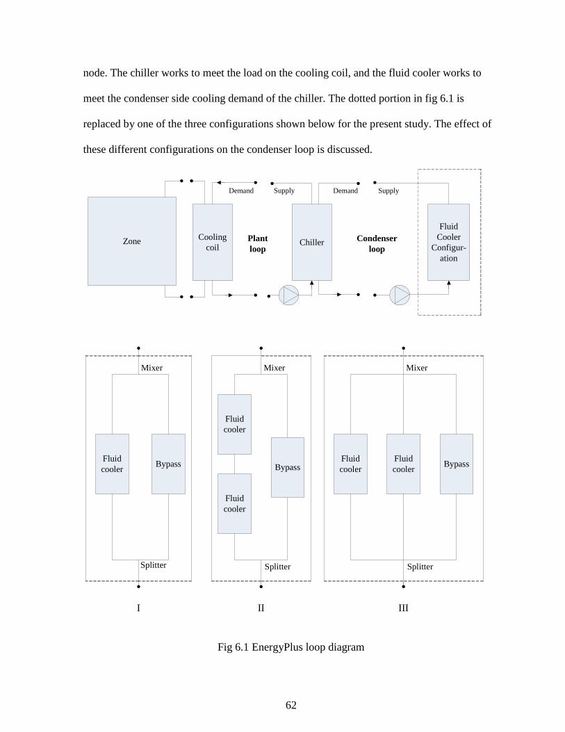
62

node. The chiller works to meet the load on the cooling coil, and the fluid cooler works to

meet the condenser side cooling demand of the chiller. The dotted portion in fig 6.1 is

replaced by one of the three configurations shown below for the present study. The effect of

these different configurations on the condenser loop is discussed.

Fig 6.1 EnergyPlus loop diagram

Zone Cooling coil

Chiller

Fluid Cooler

Configur-ation

Fluid cooler

Fluid cooler

Fluid cooler

Fluid cooler

Fluid cooler

Mixer MixerMixer

Splitter Splitter Splitter

Bypass Bypass Bypass

I II III

Condenser loop

Plant loop

SupplyDemandSupplyDemand

63

6.2 Example building and system description

Simulations were carried out for a typical office building assumed to be located at

Chicago, Illinois. Building loads simulations were run for this region for the summer design

day (21st July) and for three different configurations shown in Fig 6.1. The description of the

example building (shown in Fig 6.2) and the assumptions are listed below:

1) One story building divided into three interior conditioned zones

2) Roof with no plenum i.e. roofs are exposed to the outdoor environment

3) No ground contact (all floors are adiabatic)

4) Rectangular L-shaped building 40 ft south wall, 40 ft west wall and zone height 10

feet

5) There is a single window in the Resistive zone south wall with the window to wall

ratio approximately 0.07

6) The window is single pane 3mm clear

7) The building is oriented due north

8) Floor area is 130.1 m2 (1403 ft2)

9) The lighting loads are 18 W/m2; electrical equipment plug loads are 56.28 W/m2

10) The office occupancy is assumed to be one person per 13 m2

with a total heat gain of

131.8 Watts/Person of which 30% is assumed to be radiant heat gain

11) A water cooled chiller is used to meet the building load

64

Fig 6.2 Isometric and plan views of the building

6.3 Design day plant loop cooling demand

Fig 6.3 shows summer design day plant loop cooling demand. The peak load at

design day is approximately 18.5 KW. Building load is zero till 7 a.m. because all electric

equipments are scheduled OFF and the building is unoccupied. Starting at 7a.m. office

occupancy, lighting and all electric equipment schedules begin to ramp up. The building

cooling demand steadily increases due to the effect of increasing dry bulb temperature, solar

heat gains and scheduled loads until the activities come to an end at 5 p.m. That’s why at 5

p.m. the load in the building goes to zero.

Window

North

East

30

40

20

20

10

North

65

Fig 6.3 Plant loop cooling demand for design day

Dry fluid cooler of 93.75 KW (Heatcraft-Model 21) and Evaporative fluid cooler of

87.9 KW (Motivair Cooling Solutions-MEC0300) design capacity are taken to meet the load

requirements of the chiller. The design UA values of the fluid coolers, as calculated by

EnergyPlus, are 10674 W/K and 2753 W/K for dry and evaporative fluid coolers

respectively. Since evaporative fluid cooler model is a variable UA model; its UA value

changes at every time step depending on the location and outdoor air conditions.

6.4 Dry fluid cooler Implementation verification

This section discusses the functioning of different dry fluid cooler configurations.

Figure 6.4 shows the fluid cooler heat transfer and combined chiller condenser plus pump

heat transfer. The fluid cooler starts at 7 a.m. (43rd time step) because of sudden increase in

the building load. This causes a pick up load at the beginning. Once the system stabilizes, the

0

2000

4000

6000

8000

10000

12000

14000

16000

18000

20000

1 12 23 34 45 56 67 78 89 100 111 122 133 144

Pla

nt

loo

p c

oo

lin

g d

em

an

d (

W)

Number of timesteps in a day

66

heat transfer rate increases until 5 p.m. because of increasing load on the chiller. The system

shuts off at 5 p.m. (102nd time step) because the load in the building and hence chiller comes

to zero. The cumulative effect of chiller condenser heat transfer and pump heat addition to

the loop fluid is shown in fig 6.4. The fluid cooler rejects the heat to the outside air so that

the loop outlet temperature reaches to the set-point which is 95°F (35°C) for this case.

Fig 6.4 Condenser and pump heat addition vs. Fluid cooler heat transfer rate

6.4.1 Series configuration

Figure (6.5) shows the performance of dry fluid coolers in series configuration. The

series configuration of the fluid coolers has the set-point of 90°F (32.22°C). From the figures

it is clear that until about 12:10 p.m. (73rd time step) the first fluid cooler is able to meet the

set-point. After that, as the dry-bulb temperature of the outside air increases the heat transfer

0

5000

10000

15000

20000

25000

30000

1 12 23 34 45 56 67 78 89 100 111 122 133 144

He

at

tra

nsf

er

(W)


Error ~ 0%

Chiller

condenser +

Pump

Fluid Cooler

67

rate from the first fluid cooler decreases and loop temperature goes above the set-point. This

triggers the second fluid cooler to turn ON which was OFF till now. Because of the

combined heat transfer from both the fluid coolers, the configuration meets the set-point till

1:50 p.m. (83rd time step). Between 1:50 to 4 p.m. the dry-bulb temperature increases till 3

p.m. and then starts decreasing but it is above 31°C for the whole time. Fig 6.6 shows the

variation of dry and wet-bulb temperature for the design day. Because of the high dry-bulb

temperature, the loop temperature goes above the set-point i.e. the combined heat transfer

from both the fluid coolers can not reject heat added by chiller condenser and pump. This

situation continues until about 4:20 p.m. (98 time step). Between 4:30 to 5 p.m. the loop

temperature returns to set-point. The excess heat gained by the loop fluid between 2 to 3 p.m.

is rejected by the fluid coolers between 3 to 4:30 p.m. Finally at 5 p.m. the chiller and fluid

coolers shut off suddenly because of instant removal of loads.

(a)

0

5000

10000

15000

20000

25000

30000

1 12 23 34 45 56 67 78 89 100 111 122 133 144

He

at

tra

nsf

er

rate

(W

)


Chiller

condenser

Fluid Cooler I

Fluid Cooler II

68

(b)

Fig 6.5 Condenser vs. Fluid cooler heat transfer rate

Fig (6.6) and (6.7) show the performance of the configuration when the dry-bulb

temperature is taken as set-point. There is a high fluid cooler pick up load in the beginning

which causes the loop temperature to drop suddenly. Then the loop temperature increases as

the outdoor dry-bulb temperature increases throughout the day. Fig 6.7 shows heat transfer

rates from chiller condenser and fluid coolers. A discrepancy is found in EnergyPlus output

reporting. The condenser demand inlet temperature was not updated properly. After taking

into account the effect of lagging temperature update, the heat balance for the loop is

obtained.

0

5000

10000

15000

20000

25000

30000

1 12 23 34 45 56 67 78 89 100 111 122 133 144

He

at

tra

nsf

er

(W)


Error ~ 0%

Chiller

condenser +

PumpFluid cooler

combined

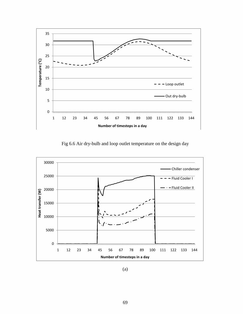
69

Fig 6.6 Air dry-bulb and loop outlet temperature on the design day

(a)

0

5

10

15

20

25

30

35

1 12 23 34 45 56 67 78 89 100 111 122 133 144

Te

mp

era

ture

(°C

)


Loop outlet

Out dry-bulb

0

5000

10000

15000

20000

25000

30000

1 12 23 34 45 56 67 78 89 100 111 122 133 144

He

at

tra

nsf

er

(W)


Chiller condenser

Fluid Cooler I

Fluid Cooler II

70

(b)

Fig 6.7 Condenser vs. Fluid cooler heat transfer rate for dry-bulb set-point

6.4.2 Parallel configuration

For the present case i.e. in parallel configuration, the total flow rate demand from

both the fluid coolers exceeds the maximum available flow rate in the loop. So the second

fluid cooler operates undersized. Fig (6.8) shows the results of parallel configuration of fluid

coolers. The set-point for the configuration is 95°F (35°C). The continuous operation of the

pump adds heat to the loop fluid. So the fluid cooler starts at 12 a.m. to remove pump heat

from the fluid. The load on the chiller, and hence on the fluid cooler, increases suddenly at 7

a.m. Fig 6.8 shows the heat balance of the operation. The configuration rejects the total heat

added by chiller and pump to the loop fluid.

0

5000

10000

15000

20000

25000

30000

1 12 23 34 45 56 67 78 89 100 111 122 133 144

He

at

tra

nsf

er

(W)


Error ~ 0.005%

Chiller condenser

+ Pump

Fluid coolers

combined +

Lagging effect

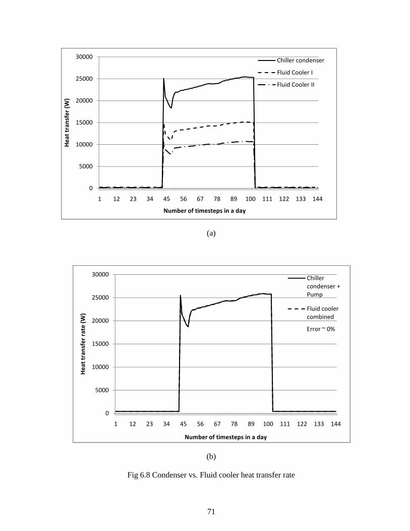
71

(a)

(b)


0

5000

10000

15000

20000

25000

30000

1 12 23 34 45 56 67 78 89 100 111 122 133 144

He

at

tra

nsf

er

(W)


Chiller condenser

Fluid Cooler I

Fluid Cooler II

0

5000

10000

15000

20000

25000

30000

1 12 23 34 45 56 67 78 89 100 111 122 133 144

He

at

tra

nsf

er

rate

(W

)


Error ~ 0%

Chiller

condenser +

Pump

Fluid cooler

combined

72

Fig 6.9 and 6.10 show the performance of the parallel dry fluid cooler configuration.

Again, as discussed for series configuration, the heat balance is obtained after accounting for

the effect of lagging temperature update. Because of pick up load in the beginning, loop

outlet temperature drops suddenly. Once the system stabilizes, the loop outlet temperature

increases as the outdoor dry-bulb temperature increases throughout the day.

Fig 6.9 Air dry-bulb and loop outlet temperature on the design day

0

5

10

15

20

25

30

35

1 12 23 34 45 56 67 78 89 100 111 122 133 144

Te

mp

era

ture

(°C

)


Loop outlet

Out dry-bulb

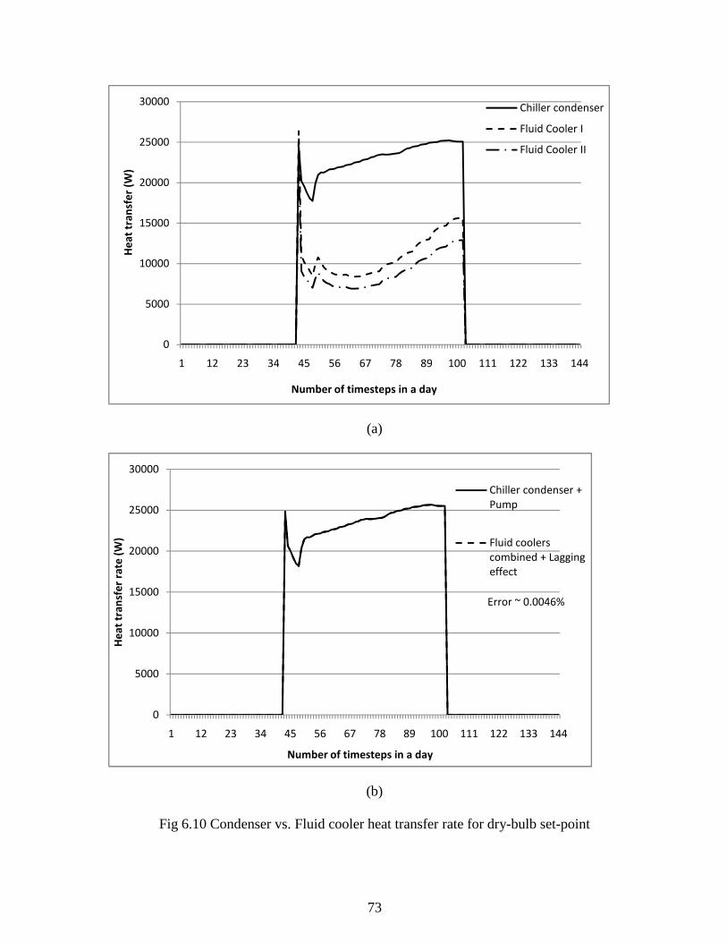
73

(a)

(b)

Fig 6.10 Condenser vs. Fluid cooler heat transfer rate for dry-bulb set-point

0

5000

10000

15000

20000

25000

30000

1 12 23 34 45 56 67 78 89 100 111 122 133 144

He

at

tra

nsf

er

(W)


Chiller condenser

Fluid Cooler I

Fluid Cooler II

0

5000

10000

15000

20000

25000

30000

1 12 23 34 45 56 67 78 89 100 111 122 133 144

He

at

tra

nsf

er

rate

(W

)


Error ~ 0.0046%

Chiller condenser +

Pump

Fluid coolers

combined + Lagging

effect

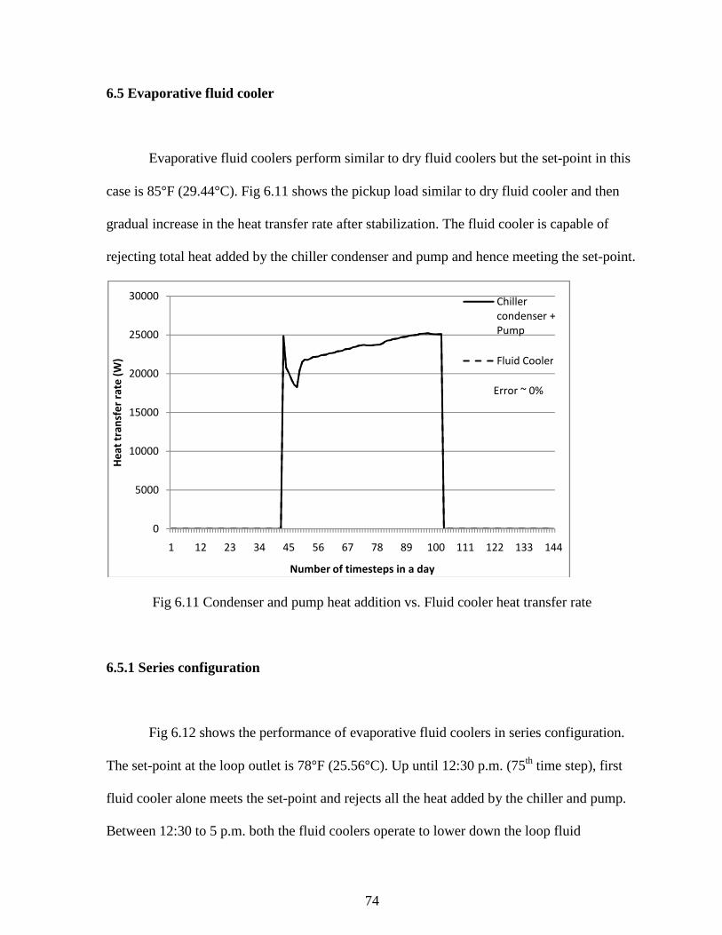
74

6.5 Evaporative fluid cooler

Evaporative fluid coolers perform similar to dry fluid coolers but the set-point in this

case is 85°F (29.44°C). Fig 6.11 shows the pickup load similar to dry fluid cooler and then

gradual increase in the heat transfer rate after stabilization. The fluid cooler is capable of

rejecting total heat added by the chiller condenser and pump and hence meeting the set-point.

Fig 6.11 Condenser and pump heat addition vs. Fluid cooler heat transfer rate

6.5.1 Series configuration

Fig 6.12 shows the performance of evaporative fluid coolers in series configuration.

The set-point at the loop outlet is 78°F (25.56°C). Up until 12:30 p.m. (75th time step), first

fluid cooler alone meets the set-point and rejects all the heat added by the chiller and pump.

Between 12:30 to 5 p.m. both the fluid coolers operate to lower down the loop fluid

0

5000

10000

15000

20000

25000

30000

1 12 23 34 45 56 67 78 89 100 111 122 133 144

He

at

tra

nsf

er

rate

(W

)


Error ~ 0%

Chiller

condenser +

Pump

Fluid Cooler

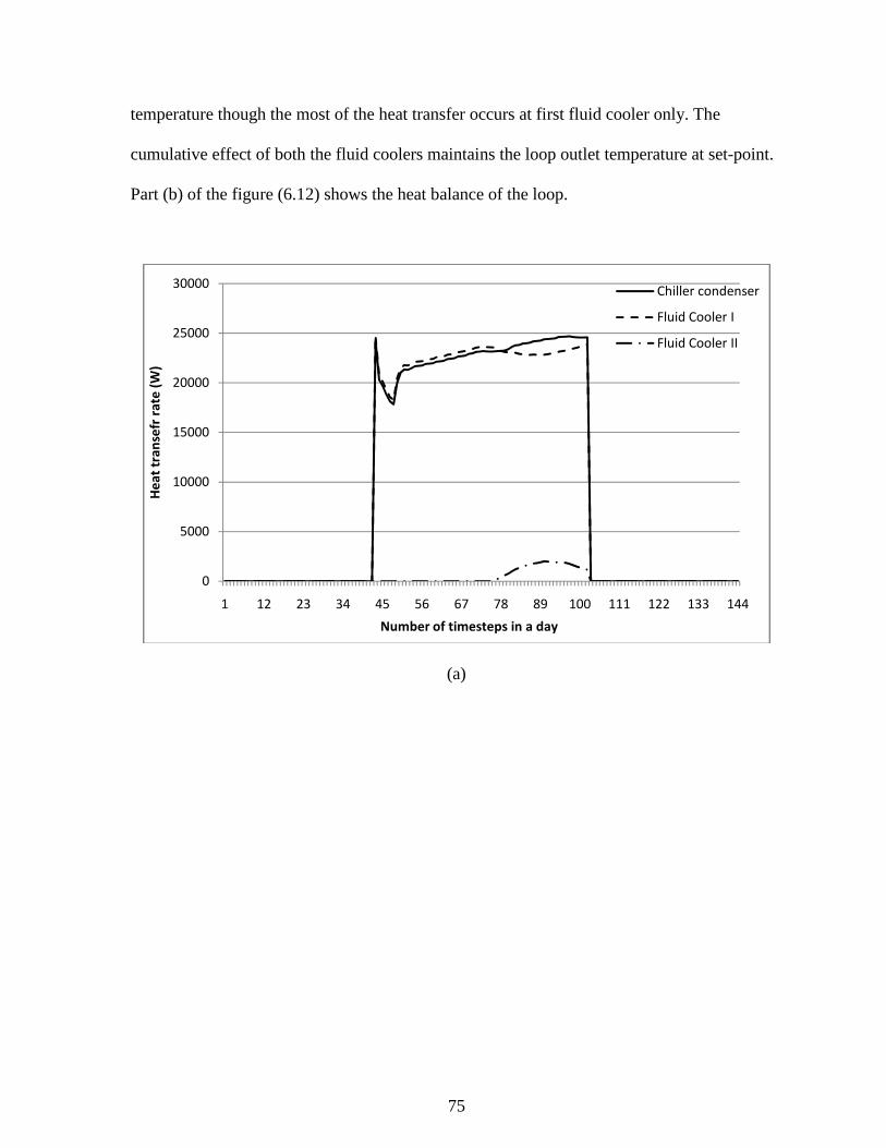
75

temperature though the most of the heat transfer occurs at first fluid cooler only. The

cumulative effect of both the fluid coolers maintains the loop outlet temperature at set-point.

Part (b) of the figure (6.12) shows the heat balance of the loop.

(a)

0

5000

10000

15000

20000

25000

30000

1 12 23 34 45 56 67 78 89 100 111 122 133 144

He

at

tra

nse

fr r

ate

(W

)


Chiller condenser

Fluid Cooler I

Fluid Cooler II

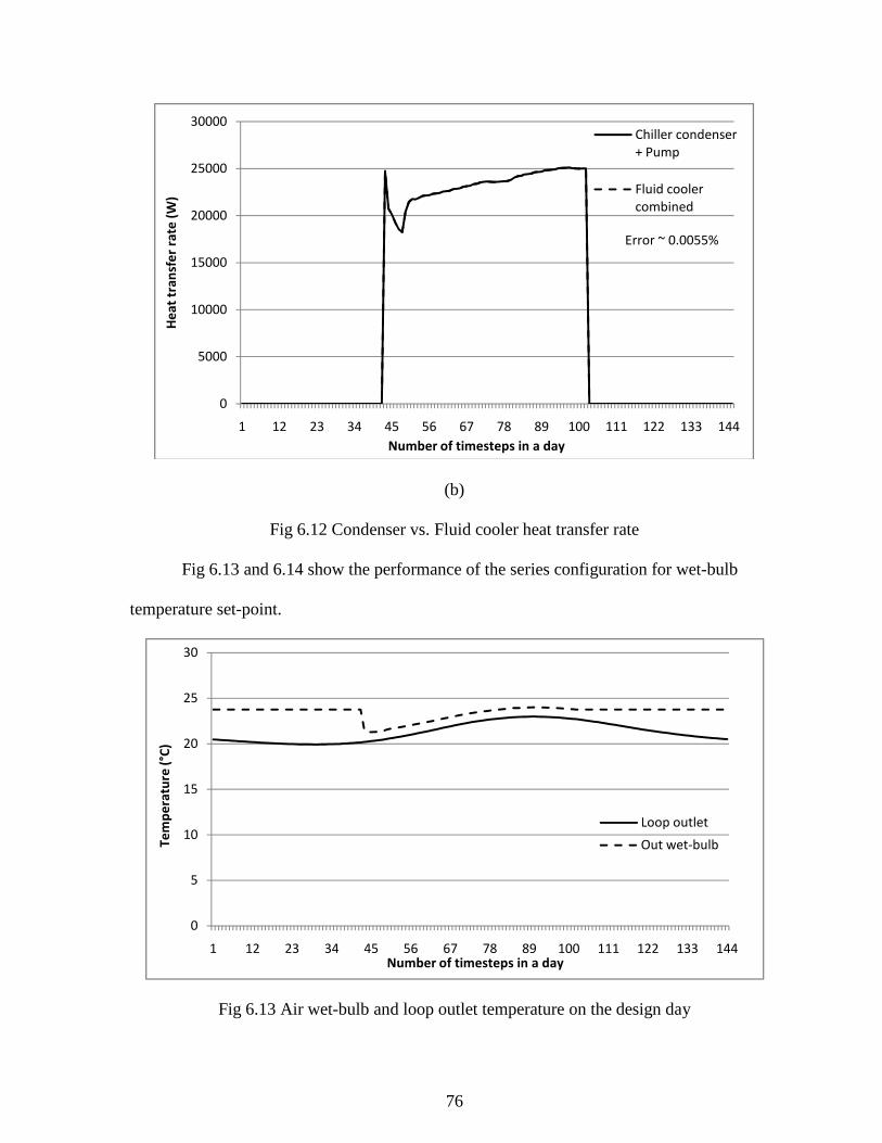
76

(b)


Fig 6.13 and 6.14 show the performance of the series configuration for wet-bulb

temperature set-point.

Fig 6.13 Air wet-bulb and loop outlet temperature on the design day

0

5000

10000

15000

20000

25000

30000

1 12 23 34 45 56 67 78 89 100 111 122 133 144

He

at

tra

nsf

er

rate

(W

)


Error ~ 0.0055%

Chiller condenser

+ Pump

Fluid cooler

combined

0

5

10

15

20

25

30

1 12 23 34 45 56 67 78 89 100 111 122 133 144

Te

mp

era

ture

(°C

)


Loop outlet

Out wet-bulb

77

(a)

(b)

Fig 6.14 Condenser vs. Fluid cooler heat transfer rate for wet-bulb set-point

0

5000

10000

15000

20000

25000

30000

1 12 23 34 45 56 67 78 89 100 111 122 133 144

He

at

tra

nsf

er

(W)


Chiller condenser

Fluid Cooler I

Fluid Cooler II

0

5000

10000

15000

20000

25000

30000

1 12 23 34 45 56 67 78 89 100 111 122 133 144

He

at

tra

nsf

er

(W)


Error ~ 0.015%

Chiller

condenser +

Pump

Fluid coolers

combined +

Lagging effect

78

6.5.2 Parallel configuration

The performance of evaporative fluid cooler for parallel configuration is shown in

figs (6.15). As explained for the dry fluid cooler parallel configuration, this configuration

turns ON at 12 a.m. because of continuous operation of the pump. Then pick up load comes

at 7 a.m. because of sudden increase in the chiller load. After the system stabilizes, heat

transfer continues to increase until 5 p.m. when the activities come to end and load on chiller

becomes zero. The combined heat addition by chiller condenser and pump is balanced by

fluid coolers as clear from the figure.

(a)

0

5000

10000

15000

20000

25000

30000

1 12 23 34 45 56 67 78 89 100 111 122 133 144

He

at

tra

nsf

er

rate

(W

)


Chiller

condenser

Fluid Cooler I

Fluid Cooler II

79

(b)


Finally, the performance of parallel configuration for wet-bulb temperature set-point

is shown below.

Fig 6.16 Air wet-bulb and loop outlet temperature on the design day

0

5000

10000

15000

20000

25000

30000

1 12 23 34 45 56 67 78 89 100 111 122 133 144

He

at

tra

nsf

er

rate

(W

)


Error ~ 0%

Chiller

condenser +

Pump

Fluid cooler

combined

0

5

10

15

20

25

30

1 12 23 34 45 56 67 78 89 100 111 122 133 144

Te

mp

era

ture

(°C

)


Loop outlet

Out wet-bulb

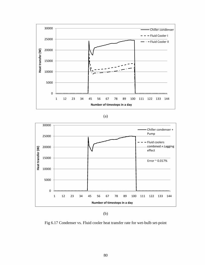
80

(a)

(b)

Fig 6.17 Condenser vs. Fluid cooler heat transfer rate for wet-bulb set-point

0

5000

10000

15000

20000

25000

30000

1 12 23 34 45 56 67 78 89 100 111 122 133 144

He

at

tra

nsf

er

(W)


Chiller condenser

Fluid Cooler I

Fluid Cooler II

0

5000

10000

15000

20000

25000

30000

1 12 23 34 45 56 67 78 89 100 111 122 133 144

He

at

tra

nsf

er

(W)


Error ~ 0.017%

Chiller condenser +

Pump

Fluid coolers

combined + Lagging

effect

81

CHAPTER VII

CONCLUSION AND RECOMMENDATION

This thesis presents development, implementation and verification of dry and evaporative

fluid cooler models in EnergyPlus. A literature review is performed to collect information

about existing fluid cooler models. The dry fluid cooler is modeled as a classis heat

exchanger by using (ℇ-NTU) method. Lebrun model is used as the basis for the evaporative

fluid cooler model. The actual model required estimation of four different parameters i.e.RK,_

, R0,_ and exponents m andn to calculate overall heat transfer coefficient (UA). This

parameter estimation could cause serious convergence problem in EnergyPlus, so the model

is modified to make it simpler to implement. In EnergyPlus, the UA value of evaporative

fluid cooler is directly calculated by iteration.

A complete validation of the fluid cooler models for part load conditions could not be

performed because of scant manufacturers’ data. In order to verify the models Lebrun model

was implemented in VBA and the results were compared with EnergyPlus results.

HVACSIM+ dry fluid cooler model (Type 762) is used to verify the EnergyPlus model. The

obtained results were in good agreements. Baltimore Aircoil provides data for multiple rating

82

points without dry-bulb temperature. A parametric study was performed to estimate the

impact of dry-bulb temperature on the output of evaporative fluid cooler models. It was

observed that even a large range of temperatures (80 to 95°F) had negligible effect on the

evaporative fluid cooler performance. The simulation results are in excellent agreement with

the catalog data. The main points of the study can be summarized as follows:

• Results of EnergyPlus dry fluid cooler model are within ±0.3% of HVACSIM+

model.

• Evaporative fluid cooler model compares very well with Lebrun model with

maximum error being less than 8%. Lebrun model itself has 7-8 % accuracy range as

compare to manufacturer’s data.

• The manufacturer’s data available for fluid coolers are seriously insufficient. Most of

the manufacturer’s don’t provide catalogue data for multiple rating points. Those who

do provide multiple rating points lack some key input parameters. Evaporative fluid

cooler model is validated against manufacturer’s data published by Baltimore Aircoil.

After obtaining the dry-bulb temperature from parametric study, simulation is

performed and the results are compared. There was a negligible deviation (0.025%

maximum) in the EnergyPlus output with respect to catalogue data.

• The results of the parametric study has shown that dry-bulb temperature affects dry-

fluid cooler results and wet-bulb temperature affects evaporative fluid cooler results

in a much higher scale than what wet-bulb temperature affects dry fluid cooler results

or dry-bulb temperature affects evaporative fluid cooler results.

83

RECOMMENDATIONS

• Experimental data sets are needed to validate part-load and off-design performance of

the models.

• Fan control strategies should be improved as per the actual control and operation

strategies of fluid cooler.

• Models to calculate evaporation losses and make up water should also be developed

and implemented.

• Dry fluid cooler model should be developed further to model “adiabatic mode”

operation.

84

REFERENCES

Facao, J. & Oliveira, A.C., Heat and mass transfer correlations for the design of small

indirect contact cooling towers, Applied Thermal Engineering 24 (2004) 1969-1978

Incropera, F. P.,DeWitt D.P. (1996), Introduction to Heat Transfer, 3 edn, John Wiley

and Sons, Hoboken, NJ.,Page no.562-563

Jang, J.Y. & Wang, Z.J., Heat and Mass transfer performances of closed type cooling

towers, Proceedings of International Conference on Advances in Computational Heat

Transfer, Palm Cove, Queensland, Australia, May 20-25th, 2001. P. 269-276

Kuester, J., and J. H. Mize. 1973. Optimization Techniques with Fortran. Chp 9.

New York, McGraw-Hill.

Lebrun, J., Silva, C Aparecida, Trebilcock, F., & Winandy, E, Simplified models for

direct and indirect contact cooling towers and evaporative condensers , Building Serv.

Eng. Res. Technol. 25,1 (2004) pp. 25-31

Mizushina, T., Ito R., & Miyashita, H., Experimental study of an evaporative cooler,

International chemical engineering 7 (4) (1967) 727-732

Parker, R.O. & Treybal, R.E., The heat and mass transfer characteristics of

evaporative coolers, Chemical Engineering Progress Symposium 57 (32) (1961)

138-149

Qureshi, B.A.& Zubair, S.M., The impact of fouling on performance evaluation of

evaporative coolers and condensers, Int J Energy Research 29 (2005) 1313-1330

85

Qureshi, B.A.& Zubair, S.M., A comprehensive design and rating study of

evaporative coolers an dcondensers. Part I. performance evaluation, International

journal of refrigeration 29 (2006) 645-658

Rosaler, R. C., 1995. Standard Handbook of Plant Engineering, 2nd Ed. McGraw-Hill,

New York, NY, pp 6-36-37.

Spitler, J.D., D.E. Fisher and D.C. Zietlow. 1989. A Primer on the Use of Influence

Coefficients in Building Energy Analysis. Proceedings of the Building Simulation '89

Conference, pp. 299-304.

Tang, Kenneth, 2005, Modeling Packaged Heat Pumps in A Quasi-Steady State

Energy Simulation Program

Xu, Xiaowei, 2007, Simulation and optimal control of hybrid ground source systems

86

APPENDIX A

Parametric study of varying dry-bulb temperature for evaporative fluid cooler model

Most of the times, evaporative fluid cooler manufacturers don’t provide dry-bulb

temperature in the catalog data. Dry-bulb temperature is required by EnergyPlus evaporative

fluid cooler model as design parameter. A parametric study is carried out to understand the

impact of dry-bulb temperature on the EnergyPlus evaporative fluid cooler results. Catalog

data presented in table 5.1 is used for the present study.

The dry-bulb temperatures are varied from 80 to 95 °F and the corresponding UA,

capacity (Q) and outlet water temperatures (Tw,out) are calculated. Table (A-1) shows the

results of the study. Data set 1 to 9 corresponds to the nine rating points shown in table 5.1.

From the table (A-1) it is clear that dry-bulb temperature does not have significant impact on

the evaporative fluid cooler simulation results.

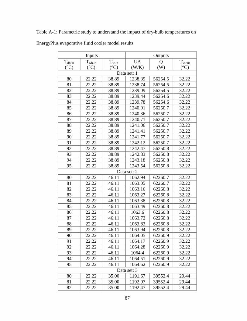
87

Table A-1: Parametric study to understand the impact of dry-bulb temperatures on

EnergyPlus evaporative fluid cooler model results

Inputs Outputs Tdb,in

(°C) Twb,in

(°C) Tw,in

(°C) UA

(W/K) Q

(W) Tw,out

(°C) Data set: 1

80 22.22 38.89 1238.39 56254.5 32.22 81 22.22 38.89 1238.74 56254.5 32.22 82 22.22 38.89 1239.09 56254.5 32.22 83 22.22 38.89 1239.44 56254.6 32.22 84 22.22 38.89 1239.78 56254.6 32.22 85 22.22 38.89 1240.01 56250.7 32.22 86 22.22 38.89 1240.36 56250.7 32.22 87 22.22 38.89 1240.71 56250.7 32.22 88 22.22 38.89 1241.06 56250.7 32.22 89 22.22 38.89 1241.41 56250.7 32.22 90 22.22 38.89 1241.77 56250.7 32.22 91 22.22 38.89 1242.12 56250.7 32.22 92 22.22 38.89 1242.47 56250.8 32.22 93 22.22 38.89 1242.83 56250.8 32.22 94 22.22 38.89 1243.18 56250.8 32.22 95 22.22 38.89 1243.54 56250.8 32.22

Data set: 2 80 22.22 46.11 1062.94 62260.7 32.22 81 22.22 46.11 1063.05 62260.7 32.22 82 22.22 46.11 1063.16 62260.8 32.22 83 22.22 46.11 1063.27 62260.8 32.22 84 22.22 46.11 1063.38 62260.8 32.22 85 22.22 46.11 1063.49 62260.8 32.22 86 22.22 46.11 1063.6 62260.8 32.22 87 22.22 46.11 1063.72 62260.8 32.22 88 22.22 46.11 1063.83 62260.8 32.22 89 22.22 46.11 1063.94 62260.8 32.22 90 22.22 46.11 1064.05 62260.9 32.22 91 22.22 46.11 1064.17 62260.9 32.22 92 22.22 46.11 1064.28 62260.9 32.22 93 22.22 46.11 1064.4 62260.9 32.22 94 22.22 46.11 1064.51 62260.9 32.22 95 22.22 46.11 1064.62 62260.9 32.22

Data set: 3 80 22.22 35.00 1191.67 39552.4 29.44 81 22.22 35.00 1192.07 39552.4 29.44 82 22.22 35.00 1192.47 39552.4 29.44

88

83 22.22 35.00 1192.88 39552.4 29.44 84 22.22 35.00 1193.28 39552.5 29.44 85 22.22 35.00 1193.69 39552.5 29.44 86 22.22 35.00 1194.09 39552.5 29.44 87 22.22 35.00 1194.5 39552.5 29.44 88 22.22 35.00 1194.91 39552.5 29.44 89 22.22 35.00 1195.32 39552.5 29.44 90 22.22 35.00 1195.72 39552.5 29.44 91 22.22 35.00 1196.13 39552.6 29.44 92 22.22 35.00 1196.54 39552.6 29.44 93 22.22 35.00 1196.96 39552.6 29.44 94 22.22 35.00 1197.37 39552.6 29.44 95 22.22 35.00 1197.78 39552.6 29.44

Data set: 4 80 25.56 35.00 939.68 23438.1 29.44 81 25.56 35.00 939.94 23438.1 29.44 82 25.56 35.00 940.2 23438.1 29.44 83 25.56 35.00 940.461 23438.1 29.44 84 25.56 35.00 940.722 23438.1 29.44 85 25.56 35.00 940.984 23438.1 29.44 86 25.56 35.00 941.246 23438.1 29.44 87 25.56 35.00 941.508 23438.1 29.44 88 25.56 35.00 941.77 23438.1 29.44 89 25.56 35.00 942.033 23438.1 29.44 90 25.56 35.00 942.296 23438.1 29.44 91 25.56 35.00 942.56 23438.1 29.44 92 25.56 35.00 942.824 23438.1 29.44 93 25.56 35.00 943.088 23438.1 29.44 94 25.56 35.00 943.352 23438.1 29.44 95 25.56 35.00 943.617 23438.2 29.44

Data set: 5 80 25.56 38.89 1097.82 42188.7 32.22 81 25.56 38.89 1098.13 42188.7 32.22 82 25.56 38.89 1098.44 42188.7 32.22 83 25.56 38.89 1098.75 42188.7 32.22 84 25.56 38.89 1099.05 42188.7 32.22 85 25.56 38.89 1099.36 42188.7 32.22 86 25.56 38.89 1099.67 42188.8 32.22 87 25.56 38.89 1099.98 42188.8 32.22 88 25.56 38.89 1100.29 42188.8 32.22 89 25.56 38.89 1100.6 42188.8 32.22 90 25.56 38.89 1100.91 42188.8 32.22 91 25.56 38.89 1101.22 42188.8 32.22 92 25.56 38.89 1101.54 42188.8 32.22 93 25.56 38.89 1101.85 42188.8 32.22

89

94 25.56 38.89 1102.16 42188.8 32.22 95 25.56 38.89 1102.48 42188.8 32.22

Data set: 6 80 25.56 46.11 845.18 43947.5 32.22 81 25.56 46.11 845.269 43947.5 32.22 82 25.56 46.11 845.358 43947.5 32.22 83 25.56 46.11 845.447 43947.5 32.22 84 25.56 46.11 845.536 43947.5 32.22 85 25.56 46.11 845.626 43947.5 32.22 86 25.56 46.11 845.715 43947.5 32.22 87 25.56 46.11 845.805 43947.5 32.22 88 25.56 46.11 845.895 43947.5 32.22 89 25.56 46.11 845.985 43947.5 32.22 90 25.56 46.11 846.075 43947.5 32.22 91 25.56 46.11 846.166 43947.5 32.22 92 25.56 46.11 846.256 43947.5 32.22 93 25.56 46.11 846.347 43947.5 32.22 94 25.56 46.11 846.438 43947.5 32.22 95 25.56 46.11 846.529 43947.5 32.22

Data set: 7 80 26.67 35.00 823.696 17579.7 29.44 81 26.67 35.00 823.246 17579.7 29.44 82 26.67 35.00 822.797 17579.7 29.44 83 26.67 35.00 822.932 17579.7 29.44 84 26.67 35.00 823.129 17579.7 29.44 85 26.67 35.00 823.326 17579.7 29.44 86 26.67 35.00 823.523 17579.7 29.44 87 26.67 35.00 823.72 17579.7 29.44 88 26.67 35.00 823.918 17579.7 29.44 89 26.67 35.00 824.116 17579.7 29.44 90 26.67 35.00 824.314 17579.7 29.44 91 26.67 35.00 824.512 17579.7 29.44 92 26.67 35.00 824.71 17579.7 29.44 93 26.67 35.00 824.909 17579.7 29.44 94 26.67 35.00 825.108 17579.7 29.44 95 26.67 35.00 825.307 17579.7 29.44

Data set: 8 80 26.67 38.89 987.458 35157.7 32.22 81 26.67 38.89 986.932 35157.7 32.22 82 26.67 38.89 986.406 35157.7 32.22 83 26.67 38.89 986.586 35157.7 32.22 84 26.67 38.89 986.839 35157.7 32.22 85 26.67 38.89 987.093 35157.7 32.22 86 26.67 38.89 987.346 35157.7 32.22 87 26.67 38.89 987.601 35157.8 32.22

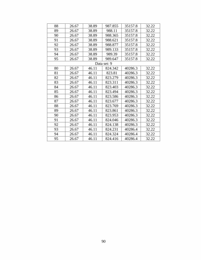
90

88 26.67 38.89 987.855 35157.8 32.22 89 26.67 38.89 988.11 35157.8 32.22 90 26.67 38.89 988.365 35157.8 32.22 91 26.67 38.89 988.621 35157.8 32.22 92 26.67 38.89 988.877 35157.8 32.22 93 26.67 38.89 989.133 35157.8 32.22 94 26.67 38.89 989.39 35157.8 32.22 95 26.67 38.89 989.647 35157.8 32.22

Data set: 9 80 26.67 46.11 824.342 40286.3 32.22 81 26.67 46.11 823.81 40286.3 32.22 82 26.67 46.11 823.279 40286.3 32.22 83 26.67 46.11 823.311 40286.3 32.22 84 26.67 46.11 823.403 40286.3 32.22 85 26.67 46.11 823.494 40286.3 32.22 86 26.67 46.11 823.586 40286.3 32.22 87 26.67 46.11 823.677 40286.3 32.22 88 26.67 46.11 823.769 40286.3 32.22 89 26.67 46.11 823.861 40286.3 32.22 90 26.67 46.11 823.953 40286.3 32.22 91 26.67 46.11 824.046 40286.3 32.22 92 26.67 46.11 824.138 40286.3 32.22 93 26.67 46.11 824.231 40286.4 32.22 94 26.67 46.11 824.324 40286.4 32.22 95 26.67 46.11 824.416 40286.4 32.22

91

APPENDIX B

Description of the VBA implementation of Lebrun model

Lebrun model described in chapter 2 was implemented in VBA to verify EnergyPlus

evaporative fluid cooler model. A parameter estimation tool, developed by Kenneth Tang

(2005) for water to air heat pumps, was used as the basis to develop this model. All the four

parameters, which are RK,_ , R0,_ and exponents m andn required by Lebrun model, are

estimated by using a parameter estimation tool. Once the parameters are determined, the

capacity of the fluid cooler is calculated. The obtained capacities are in excellent agreement

with the publish capacities.

Methodology

Figure B-1 below shows the flow chart of the VBA algorithm of the Lebrun model.

To start with, an initial guess of all the four parameters was entered by the user. The model

then guesses the outlet fluid cooler wet-bulb temperature and estimates the effectiveness of

the fluid cooler. By using this effectiveness, cooling capacity of the fluid cooler is calculated.

92

This cooling capacity is then used to calculate again the wet-bulb temperature at fluid cooler

exit. If the difference between the guess value and calculated of exiting wet-bulb temperature

is more than the tolerance limit then iterations are performed until the convergence on the

wet-bulb temperature value is obtained.

Fig B-1: Flow chart of Lebrun model implemented in VBA

Initial guess: Ran, Rwn, m and n

ABS(twb,ex,guess-twb,ex) < err

yes

no

Data from catalog data:tw,su, twb,su,Q,Va,Vw

Initial guess: twb,ex,guess

Calculate exhaust air enthalpy

Calculate twb,ex

Calculate heating capacity (Q)

Calculate effectiveness

Calculate global heat transfer coefficient

Calculate specific heat of fictitious air (cp,af)

Converge on the error, Eq. (B-1)

Output:Optimal values of Ran, Rwn, m, n and Q

no

yes

New estimation of parameters using Nelder

Mead Simplex

twb,ex,guess = twb,ex

93

Where,

t = temperature (°C)

V= Volumetric flow rate (m3/s)

Q = Cooling capacity (W)

cp = specific heat capacity of water (kJ/kg-K)

err = tolerance of wet-bulb temperature

Subscripts

a = air

ex= exiting

su =supply

w= water

wb= wet-bulb

guess = guessed value

f = fictitious

Once the exiting wet-bulb temperature is fixed, the model uses corresponding cooling

capacity to calculate the following objective function:

Z � ∑ xªobeb�c¥$^'(ªob�od�be}~$^'ªobeb�c¥$^' y

M{̂«@ � Acc (B-1)

Where,

N= number of data set from catalog

Q-K3K�\¬ = Catalog cooling capacity (W)

Q-K�-]�K3N� = Calculated cooling capacity (W)

Acc = accuracy of the Nelder Mead routine given by the user

94

Nelder Mead Simplex is used to make new guess of parameters until the value of the

above objective function is obtained as less than specified accuracy. Kuester and Mize (1973)

implemented the Nelder Mead Simplex into FORTRAN which is the basis of VBA routine of

Nelder Mead Simplex used for the present study. For each set of guessed parameters, new

exiting wet-bulb temperature is calculated and subsequently cooling capacity and the

objective function is calculated. Once the objective function value becomes less than the

accuracy, the parameters are reported in the output. The parameters are then used to calculate

the cooling capacity for different rating points. The source code of the Lebrun model is

shown below.

Source code

'INPUT FROM CATALOG 'InletAirWetbulbTemp = inlet air dry bulb temperature (C) 'AirVolFlowRate = Volumetric air flow rate (m^3) 'CoolingCapacity = cooling capacity (KW) 'InletWaterTemp = inlet water temperature (C) 'VS = source side volumetric water flow rate (m^3) Sub Main() Dim accuracy As Double, n As Integer,X() As Double, np As Integer, StartTime_ As Single, FinishTime As Single, TotalTime As Single Dim i As Integer, guessnum As Integer StartTime = Timer 'Start Time of the simulation accuracy = Worksheets("ParameterEstimator").Cells(1, 2) 'Accuracy for Nelder Mead n = Worksheets ("ParameterEstimator").Cells(2, 2) 'Number of Data Set from catalog fluidtype = Worksheets("ParameterEstimator").Cells(3, 2) 'Fluid Type 0 or 1 '(Currently 0 is valid fluid type) guessnum = Worksheets("ParameterEstimator").Cells(10, 3) 'Set of guessed parameters np = 4 'Numbers of parameters ReDim InletAirWetbulbTemp(n) As Single, AirVolFlowRate(n) As Single, CoolingCapacity(n) As Single, InletWaterTemp(n) As Single, WaterVolFlowRate(n)_ As Single ReDim X(np + 1, np) As Double '=============READING INPUT DATA=============== 'Read in the catalog data input For i = 1 To n InletAirWetbulbTemp(i) = Worksheets("InputData"). Cells_ (T2firstrow + i - 1, T2firstcol)

95

AirVolFlowRate(i) = Worksheets("InputData").Cells_ (T2firstrow + i - 1, T2firstcol + 1) CoolingCapacity(i) = Worksheets ("InputData").Cells_ (T2firstrow + i - 1, T2firstcol + 2) InletWaterTemp(i) = Worksheets("InputData").Cells_ (T2firstrow + i - 1, T2firstcol + 3) WaterVolFlowRate(i) = Worksheets("InputData").Cells_ (T2firstrow + i - 1, T2firstcol + 4) Next i 'Check if the input data is entered If AirVolFlowRate(1) = 0 Then MsgBox "No input data is entered. Check Worksheet 'INPUT'." Exit Sub End If '===============GENERATING PARAMETERS============== 'Status of the simulation Application.DisplayStatusBar = True Application.StatusBar = "SIMULATION STATUS: Reading Input_ Data & Generating Parameters" 'Read initial guess of parameters For i = 1 To np X(1, i) = Worksheets("ParameterEstimator").Cells(14 + i, guessnum + 1) Next i 'Check if the initial guess is entered If X(1, 1) = 0 Then MsgBox "No initial guess of parameters entered. Check initial guess number." Exit Sub End If Call NelderMead(n, X(), np, accuracy) Call MI(guessnum, n, np, X()) 'Print the parameters generated from Nelder Mead For i = 1 To np Worksheets("ParameterEstimator").Cells(20 + i, guessnum + 1) = X(np + 1, i) Next i 'Analyze the result and calculating errors Call ResultAnalyst(guessnum, n) 'Status of the simulation FinishTime = Timer 'End Time of the simulation TotalTime = FinishTime - StartTime Application.StatusBar = "SIMULATION STATUS: Ended Succesfully Simulation Time=" & TotalTime & " Seconds" End Sub Sub ResultAnalyst(guessnum As Integer, n As Integer) ‘Author: Keneth Tang Dim j As Integer, i As Integer, error As Single, p As_ Single, q As Single 'Calculate %error and write to Worksheet "Result" For i = 1 To n error = 100 * (Worksheets("RESULT").Cells(4 + i, 3 + 2 * (guessnum - 1))_ - Worksheets("RESULT").Cellserror Next i Worksheets("ParameterEstimator").Cells(27, guessnum + 1) = RMSError(guessnum,_ n,

1)

96

'Calculate RMS error for CoolingCapacity Worksheets("ParameterEstimator").Cells(28, guessnum + 1) = _ PercentageRMSError(guessnum, n, 1) 'Calculate %RMS error for W Worksheets("ParameterEstimator").Cells(29, guessnum + 1) = _ AverageError(guessnum, n, 1) End Sub Sub NelderMead(n As Integer, X() As Double, np As Integer, ACC As Double) ‘Author: Keneth Tang Dim NP1 As Integer, q As Single, p As Single, M As Integer, i As Integer, j As_ Integer, AP As Integer, ITR As Integer,_ Z() As Double,Dim ZHI As Double, ZLO_ As Double, k As_ Integer, EN As Integer, SUM As Double, EJ As Double, L As_ Integer, ZCEN As Double, ZREF As Double, ZCON As Double,_ZEX As Double ReDim XCEN(np + 1, np) As Double, XREF(np + 1, np) As Double, XCON(np + 1, np)_ As Double, XEX(np + 1, np) As_ Double, Z(np + 1) As Double Const ITMAX As Single = 1000 'Max number of iteration Const ALFA As Single = 1 'Reflection coefficient ALFA>0 Const BETA As Single = 0.5'Contraction coefficient 0<BETA<1 Const GAM As Single = 2 'Expansion coefficient Const A As Single = 0.1 Open "NM_OUPUT.txt" For Output As #1 NP1 = np + 1 q = (A / np * (2 ^ 0.5)) * ((np + 1) ^ 0.5 - 1) p = (A / np * (2 ^ 0.5)) * ((np + 1) ^ 0.5 + np - 1) M = np + 1 For i = 2 To M AP = 1 For j = 1 To np AP = AP + 1 If (i = AP) Then X(i, j) = X(1, j) + p Else X(i, j) = X(1, j) + q End If Next j Next i Write #1, Tab(3); "NELDER MEAD OPTIMIZATIION" Write #1, "N=", n; Tab(10); "ACC="; ACC; Tab(30); "ALFA="; ALFA; Tab(42); "BETA="; BETA; Tab(56); "GAM="; GAM Write #1, Write #1, "Starting Simplex" Write #1, "----------------------------------" Write #1, '-------------BEGIN NELDER MEAD ROUTINE------------- ITR = 0 150 For i = 1 To NP1 Call PE1(n, i, X(), Z(), np, NP1) Next i ITR = ITR + 1 If (ITR >= ITMAX) Then GoTo 145 158 Write #1, "Iteration Number", ITR

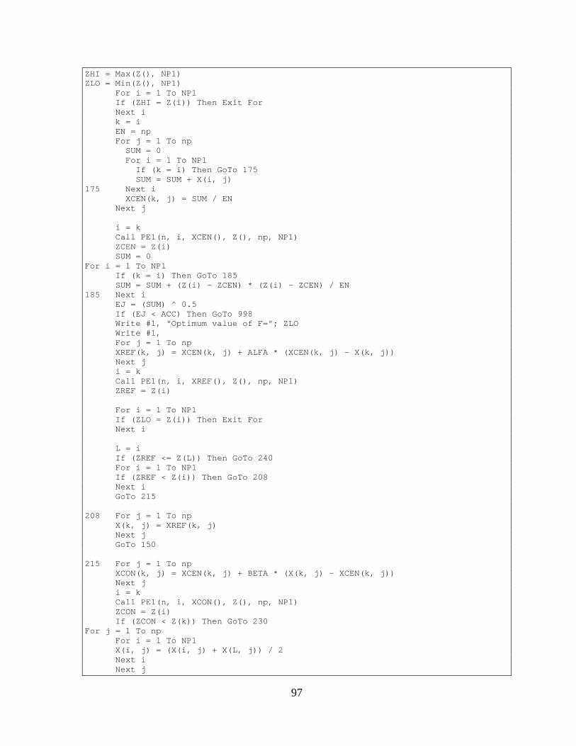
97

ZHI = Max(Z(), NP1) ZLO = Min(Z(), NP1) For i = 1 To NP1 If (ZHI = Z(i)) Then Exit For Next i k = i EN = np For j = 1 To np SUM = 0 For i = 1 To NP1 If (k = i) Then GoTo 175 SUM = SUM + X(i, j) 175 Next i XCEN(k, j) = SUM / EN Next j i = k Call PE1(n, i, XCEN(), Z(), np, NP1) ZCEN = Z(i) SUM = 0 For i = 1 To NP1 If (k = i) Then GoTo 185 SUM = SUM + (Z(i) - ZCEN) * (Z(i) - ZCEN) / EN 185 Next i EJ = (SUM) ^ 0.5 If (EJ < ACC) Then GoTo 998 Write #1, "Optimum value of F="; ZLO Write #1, For j = 1 To np XREF(k, j) = XCEN(k, j) + ALFA * (XCEN(k, j) - X(k, j)) Next j i = k Call PE1(n, i, XREF(), Z(), np, NP1) ZREF = Z(i) For i = 1 To NP1 If (ZLO = Z(i)) Then Exit For Next i L = i If (ZREF <= Z(L)) Then GoTo 240 For i = 1 To NP1 If (ZREF < Z(i)) Then GoTo 208 Next i GoTo 215 208 For j = 1 To np X(k, j) = XREF(k, j) Next j GoTo 150 215 For j = 1 To np XCON(k, j) = XCEN(k, j) + BETA * (X(k, j) - XCEN(k, j)) Next j i = k Call PE1(n, i, XCON(), Z(), np, NP1) ZCON = Z(i) If (ZCON < Z(k)) Then GoTo 230 For j = 1 To np For i = 1 To NP1 X(i, j) = (X(i, j) + X(L, j)) / 2 Next i Next j

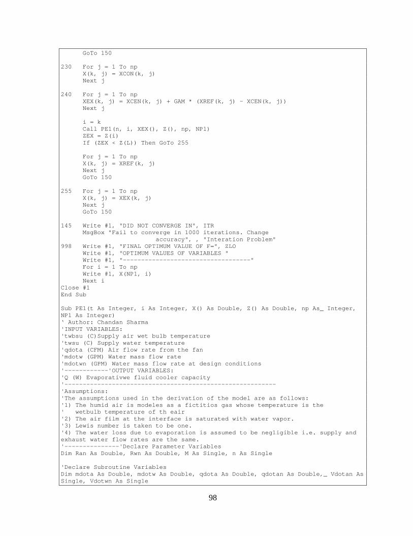
98

GoTo 150 230 For j = 1 To np X(k, j) = XCON(k, j) Next j 240 For j = 1 To np XEX(k, j) = XCEN(k, j) + GAM * (XREF(k, j) - XCEN(k, j)) Next j i = k Call PE1(n, i, XEX(), Z(), np, NP1) ZEX = Z(i) If (ZEX < Z(L)) Then GoTo 255 For j = 1 To np X(k, j) = XREF(k, j) Next j GoTo 150 255 For j = 1 To np X(k, j) = XEX(k, j) Next j GoTo 150 145 Write #1, "DID NOT CONVERGE IN", ITR MsgBox "Fail to converge in 1000 iterations. Change accuracy", , "Interation Problem" 998 Write #1, "FINAL OPTIMUM VALUE OF F=", ZLO Write #1, "OPTIMUM VALUES OF VARIABLES " Write #1, "-----------------------------------" For i = 1 To np Write #1, X(NP1, i) Next i Close #1 End Sub Sub PE1(t As Integer, i As Integer, X() As Double, Z() As Double, np As_ Integer, NP1 As Integer) ‘ Author: Chandan Sharma 'INPUT VARIABLES: 'twbsu (C)Supply air wet bulb temperature 'twsu (C) Supply water temperature 'qdota (CFM) Air flow rate from the fan 'mdotw (GPM) Water mass flow rate 'mdotwn (GPM) Water mass flow rate at design conditions '------------'OUTPUT VARIABLES: 'Q (W) Evaporativwe fluid cooler capacity '---------------------------------------------------------- 'Assumptions: 'The assumptions used in the derivation of the model are as follows: '1) The humid air is modeles as a fictitios gas whose temperature is the ' wetbulb temperature of th eair '2) The air film at the interface is saturated with water vapor. '3) Lewis number is taken to be one. '4) The water loss due to evaporation is assumed to be negligible i.e. supply and exhaust water flow rates are the same. '---------------'Declare Parameter Variables Dim Ran As Double, Rwn As Double, M As Single, n As Single 'Declare Subroutine Variables Dim mdota As Double, mdotw As Double, qdota As Double, qdotan As Double,_ Vdotan As Single, Vdotwn As Single

99

Dim mdotan As Double, mdotwn As Double Dim twbsu As Single, twbex As Single, twsu As Single, twex_ As Single, haex As_ Double, hasu As Double, twbexlast As_ Double, Dim cpaf As Double, cpr As_ Double, Caf As Double, Dim Cr As Double, Dim Cmin As Double, Cmax As Double Dim Rw As Double, Ra As Double, Rfic As Double, Raf As_ Double, Dim AUfic As_ Double, NTUfic As Double Dim C As Double, q As Double, E As Double Dim C0 As Single, C1 As Single, C2 As Single, C3 As Single Dim cpa As Single, Dim iter As Integer, Dim diff As Single Dim density As Single, Dim WCP As Single, Dim k As Integer '---------------------------------------------------------- 'mdota : Air mass flow rate (kg/s) 'qdota : Air volumetric flow rate (CFM) 'qdotan: Air volumetric flow rate at nominal conditions(CFM) 'mdotw : Water mass flow rate in the tube i.e. process 'fluid flow rate (GPM) 'mdotan: Air mass flow rate at nominal conditions (kg/s) 'mdotwn: Water mass flow rate at nominal conditions (GPM) 'twbsu : Supply or inlet air wetbulb temperature (C) 'twsu : Supply or inlet water temperature (C) 'twex : Exit or outlet water temperature (C) 'hasu : Supply or inlet air enthalpy (j/kg) 'haex : Exhaust air enthalpy (j/kg) 'cpaf : Specific heat for fictitious air (j/kg-k) 'cpr : Specific heat for water or process fluid (j/kg-k) 'Caf : Capacity for fictitious air (W/K) 'Cr : Capacity for water or process fluid (W/K) 'Ra : Air resistance (m2-K/W) 'Rw : Water or process fluid resistance (m2-K/W) 'Ran : Air resistance at nominal conditions (m2-K/W) Rwn : Water or process fluid resistance at nominal 'conditions (m2-K/W) 'AUfic : Heat transfer coefficient for fictitious air (W/K) 'e : Effectiveness of the heat exchanger 'Q : Capacity/Heat transfer rate of the Evaporative 'fluid cooler (W) 'M=Refrigerant side mass flow rate ratio exponent 'n=Air side mass flow rate ratio exponent '---------------------------------------------------------- C0 = 9362.5 ' c0,c1,c2 and c3 are polynomial coefficients for h=f(twb), which ' depend on atmospheric pressure C1 = 1786.1 C2 = 11.35 C3 = 0.98855 Vdotan = Worksheets("ParameterEstimator").Cells(4, 2).VALUE Vdotwn = Worksheets("ParameterEstimator").Cells(5, 2).VALUE 'The following parameters are calculated for Baltimore 'Aircoil closed circuit 'cooling tower V-series Ran = X(i, 1) ^ 2 Rwn = X(i, 2) ^ 2 M = X(i, 3) ^ 2 n = X(i, 4) ^ 2 Z(i) = 0 For k = 1 To t twbsu = InletAirWetbulbTemp(k) 'Using the polynomial function calculate the supply/inlet 'air enthalpy hasu = C0 + C1 * twbsu + C2 * twbsu ^ 2 + C3 * twbsu ^ 3 cpa = 1.0057 'Air specific heat (kj/kg-k) 'Guess the exhaust air wetbulb temperature twbex = twbsu + 7 Call AirDensity(twbsu, density)

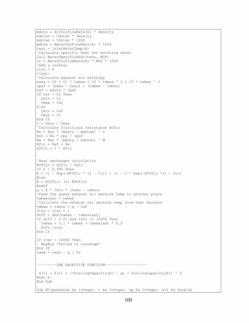
100

mdota = AirVolFlowRate(k) * density mdotan = Vdotan * density mdotwn = Vdotwn * 1000 mdotw = WaterVolFlowRate(k) * 1000 twsu = InletWaterTemp(k) 'Calculate specific heat for entering water Call WaterSpecificHeat(twsu, WCP) Cr = WaterVolFlowRate(k) * WCP * 1000 'Add a counter iter = 0 line1: 'Calculate exhaust air enthalpy haex = C0 + C1 * twbex + C2 * twbex ^ 2 + C3 * twbex ^ 3 cpaf = (haex - hasu) / (twbex - twbsu) Caf = mdota * cpaf If Caf > Cr Then Cmin = Cr Cmax = Caf Else Cmin = Caf Cmax = Cr End If C = Cmin / Cmax 'Calculate fictitious resistance AUfic Ra = Ran * (mdota / mdotan) ^ n Raf = Ra * cpa / cpaf Rw = Rwn * (mdotw / mdotwn) ^ M Rfic = Raf + Rw AUfic = 1 / Rfic 'Heat exchanger calculation NTUfic = AUfic / Cmin If C > 0.995 Then E = (1 - Exp(-NTUfic * (1 - C))) / (1 - C * Exp(-NTUfic *(1 - C))) Else E = NTUfic/ (1+ NTUfic) Endif q = E * Cmin * (twsu - twbsu) 'Pass the guess exhaust air wetbulb temp to another place twbexlast = twbex 'Calculate the exhaust air wetbulb temp from heat balance twbex = twbsu + q / Caf iter = iter + 1 diff = Abs(twbex - twbexlast) If diff > 0.01 And iter <= 10000 Then twbex = 0.1 * twbex + twbexlast * 0.9 GoTo line1 End If If iter > 10000 Then MsgBox "Failed to converge" End If twex = twsu - q / Cr '--------THE OBJECTIVE FUNCTION------------------- Z(i) = Z(i) + ((CoolingCapacity(k) - q) / CoolingCapacity(k)) ^ 2 Next k End Sub Sub MI(guessnum As Integer, t As Integer, np As Integer, X() As Double)

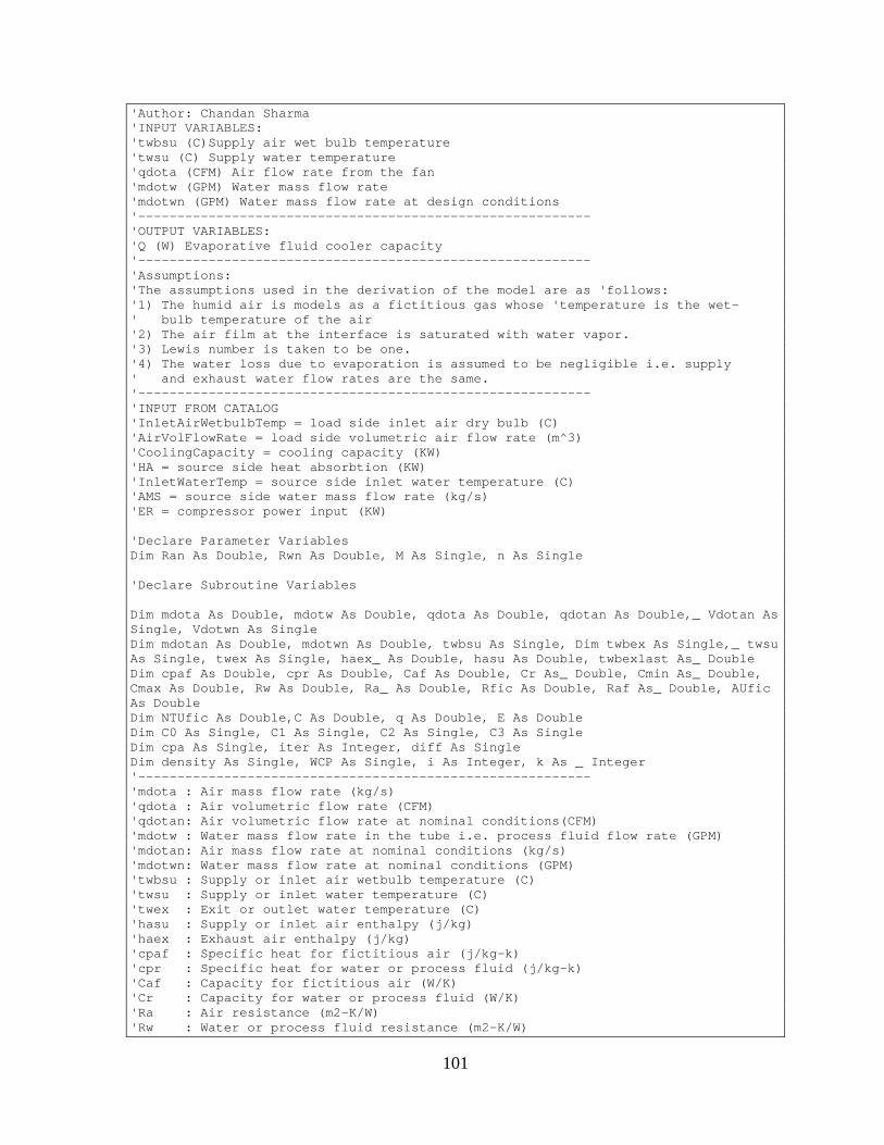
101

'Author: Chandan Sharma 'INPUT VARIABLES: 'twbsu (C)Supply air wet bulb temperature 'twsu (C) Supply water temperature 'qdota (CFM) Air flow rate from the fan 'mdotw (GPM) Water mass flow rate 'mdotwn (GPM) Water mass flow rate at design conditions '---------------------------------------------------------- 'OUTPUT VARIABLES: 'Q (W) Evaporative fluid cooler capacity '---------------------------------------------------------- 'Assumptions: 'The assumptions used in the derivation of the model are as 'follows: '1) The humid air is models as a fictitious gas whose 'temperature is the wet- ' bulb temperature of the air '2) The air film at the interface is saturated with water vapor. '3) Lewis number is taken to be one. '4) The water loss due to evaporation is assumed to be negligible i.e. supply ' and exhaust water flow rates are the same. '---------------------------------------------------------- 'INPUT FROM CATALOG 'InletAirWetbulbTemp = load side inlet air dry bulb (C) 'AirVolFlowRate = load side volumetric air flow rate (m^3) 'CoolingCapacity = cooling capacity (KW) 'HA = source side heat absorbtion (KW) 'InletWaterTemp = source side inlet water temperature (C) 'AMS = source side water mass flow rate (kg/s) 'ER = compressor power input (KW) 'Declare Parameter Variables Dim Ran As Double, Rwn As Double, M As Single, n As Single 'Declare Subroutine Variables Dim mdota As Double, mdotw As Double, qdota As Double, qdotan As Double,_ Vdotan As Single, Vdotwn As Single Dim mdotan As Double, mdotwn As Double, twbsu As Single, Dim twbex As Single,_ twsu As Single, twex As Single, haex_ As Double, hasu As Double, twbexlast As_ Double Dim cpaf As Double, cpr As Double, Caf As Double, Cr As_ Double, Cmin As_ Double, Cmax As Double, Rw As Double, Ra_ As Double, Rfic As Double, Raf As_ Double, AUfic As Double Dim NTUfic As Double,C As Double, q As Double, E As Double Dim C0 As Single, C1 As Single, C2 As Single, C3 As Single Dim cpa As Single, iter As Integer, diff As Single Dim density As Single, WCP As Single, i As Integer, k As _ Integer '---------------------------------------------------------- 'mdota : Air mass flow rate (kg/s) 'qdota : Air volumetric flow rate (CFM) 'qdotan: Air volumetric flow rate at nominal conditions(CFM) 'mdotw : Water mass flow rate in the tube i.e. process fluid flow rate (GPM) 'mdotan: Air mass flow rate at nominal conditions (kg/s) 'mdotwn: Water mass flow rate at nominal conditions (GPM) 'twbsu : Supply or inlet air wetbulb temperature (C) 'twsu : Supply or inlet water temperature (C) 'twex : Exit or outlet water temperature (C) 'hasu : Supply or inlet air enthalpy (j/kg) 'haex : Exhaust air enthalpy (j/kg) 'cpaf : Specific heat for fictitious air (j/kg-k) 'cpr : Specific heat for water or process fluid (j/kg-k) 'Caf : Capacity for fictitious air (W/K) 'Cr : Capacity for water or process fluid (W/K) 'Ra : Air resistance (m2-K/W) 'Rw : Water or process fluid resistance (m2-K/W)

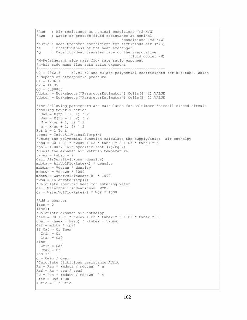
102

'Ran : Air resistance at nominal conditions (m2-K/W) 'Rwn : Water or process fluid resistance at nominal 'conditions (m2-K/W) 'AUfic : Heat transfer coefficient for fictitious air (W/K) 'e : Effectiveness of the heat exchanger 'Q : Capacity/Heat transfer rate of the Evaporative 'fluid cooler (W) 'M=Refrigerant side mass flow rate ratio exponent 'n=Air side mass flow rate ratio exponent '---------------------------------------------------------- C0 = 9362.5 ' c0,c1,c2 and c3 are polynomial coefficients for h=f(twb), which ' depend on atmospheric pressure C1 = 1786.1 C2 = 11.35 C3 = 0.98855 Vdotan = Worksheets("ParameterEstimator").Cells(4, 2).VALUE Vdotwn = Worksheets("ParameterEstimator").Cells(5, 2).VALUE 'The following parameters are calculated for Baltimore 'Aircoil closed circuit 'cooling tower V-series Ran = X(np + 1, 1) ^ 2 Rwn = X(np + 1, 2) ^ 2 M = X(np + 1, 3) ^ 2 n = X(np + 1, 4) ^ 2 For k = 1 To t twbsu = InletAirWetbulbTemp(k) 'Using the polynomial function calculate the supply/inlet 'air enthalpy hasu = C0 + C1 * twbsu + C2 * twbsu ^ 2 + C3 * twbsu ^ 3 cpa = 1.0057 'Air specific heat (kj/kg-k) 'Guess the exhaust air wetbulb temperature twbex = twbsu + 7 Call AirDensity(twbsu, density) mdota = AirVolFlowRate(k) * density mdotan = Vdotan * density mdotwn = Vdotwn * 1000 mdotw = WaterVolFlowRate(k) * 1000 twsu = InletWaterTemp(k) 'Calculate specific heat for entering water Call WaterSpecificHeat(twsu, WCP) Cr = WaterVolFlowRate(k) * WCP * 1000 'Add a counter iter = 0 line1: 'Calculate exhaust air enthalpy haex = C0 + C1 * twbex + C2 * twbex ^ 2 + C3 * twbex ^ 3 cpaf = (haex - hasu) / (twbex - twbsu) Caf = mdota * cpaf If Caf > Cr Then Cmin = Cr Cmax = Caf Else Cmin = Caf Cmax = Cr End If C = Cmin / Cmax 'Calculate fictitious resistance AUfic Ra = Ran * (mdota / mdotan) ^ n Raf = Ra * cpa / cpaf Rw = Rwn * (mdotw / mdotwn) ^ M Rfic = Raf + Rw AUfic = 1 / Rfic

103

'Heat exchanger calculation NTUfic = AUfic / Cmin If C > 0.995 Then E = (1 - Exp(-NTUfic * (1 - C))) / (1 - C * Exp(-NTUfic *(1 - C))) Else E = NTUfic/ (1+ NTUfic) Endif q = E * Cmin * (twsu - twbsu) 'Pass the guess exhaust air wetbulb temp to another place twbexlast = twbex 'Calculate the exhaust air wetbulb temp from heat balance twbex = twbsu + q / Caf iter = iter + 1 diff = Abs(twbex - twbexlast) If diff > 0.01 And iter <= 10000 Then twbex = 0.1 * twbex + twbexlast * 0.9 GoTo line1 End If If iter > 10000 Then MsgBox "Failed to converge" End If twex = twsu - q / Cr Worksheets("RESULT").Cells(4 + k, 3 + 2 * (guessnum - 1)) = q Next k End Sub Sub AirDensity(t As Single, density As Single) ‘Author: Jeff D. Spitler 'returns air density in kg/m3 when given 'T in C Dim p As Single, R As Single, T_K As Single p = 101.325 'kpa R = 0.28704 T_K = t + 273.15 density = p / (R * T_K) End Sub Sub WaterSpecificHeat(TW As Single, WCP As Single) 'Author: Jeff D. Spitler '--------------------------------------------------------- 'Specific heat of water at 1 atmosphere, 0 to 100 C. 'Equation from linear 'least-squares regression of data from 'CRC Handbook '(op.cit.)page D-174; in 'J/g-C (or kJ/kg-C). 'For temps > 100, fit to data from Karlekar & Desmond '(saturated). Dim ACP0 As Single, ACP1 As Double, ACP2 As Double, ACP3 As Single, ACP4 As_ Double, ACP5 As Single, ACP6 As Single,_ ACP7 As Single, ACP8 As Double ACP0 = 4.21534 ACP1 = -0.00287819 ACP2 = 0.000074729 ACP3 = -0.000000779624 ACP4 = 0.000000003220424 ACP5 = 2.9735 ACP6 = 0.023049 ACP7 = -0.00013953 ACP8 = 0.000000309247 WCP = ACP0 + TW * ACP1 + (TW ^ 2) * ACP2 + (TW ^ 3) * ACP3 + (TW ^ 4) * ACP4 If (TW > 100) Then WCP = ACP5 + TW * ACP6 + (TW ^ 2) * ACP7 + (TW ^ 3) * ACP8 'Return End Sub

104

VITA

Chandan Sharma

Candidate for the Degree of

Master of Science Thesis: DEVELOPMENT OF DRY AND EVAPORATIVE FLUID COOLER MODELS

FOR ENERGYPLUS Major Field: Mechanical Engineering Biographical:

Education: Completed the requirements for the Master of Science in Mechanical Engineering at Oklahoma State University, Stillwater, Oklahoma in December, 2009.

ADVISER’S APPROVAL: Dr. Daniel E. Fisher

Name: Chandan Sharma Date of Degree: December, 2009 Institution: Oklahoma State University Location: Stillwater, Oklahoma Title of Study: DEVELOPMENT OF DRY AND EVAPORATIVE FLUID COOLER

MODELS FOR ENERGYPLUS Pages in Study: 116 Candidate for the Degree of Master of Science

Major Field: Mechanical Engineering Dry and evaporative fluid cooler models were developed and implemented in the EnergyPlus simulation environment. First, the operation of the fluid coolers and a comparison with cooling towers were presented. The literature review has shown various models of the fluid coolers. The Lebrun model was chosen as the basis for evaporative fluid cooler model whiles the ℇ-NTU correlation for cross flow heat exchanger with both streams unmixed was used for the dry fluid cooler model. The model sensitivity for various input parameters has been analyzed. The evaporative fluid cooler model was validated by using manufacturer’s catalog data. The HVACSIM+ dry fluid cooler model (type 762) was used to verify the EnergyPlus dry fluid cooler model. Similarly, The Lebrun model was implemented in VBA to verify EnergyPlus evaporative fluid cooler model. The new models produced results that were comparable to previous models. The implementation of the models was also verified by arranging them in series and parallel configurations and analyzing their performance. The models performed as expected for both the configurations.

DEVELOPMENT OF DRY AND EVAPORATIVE FLUID...

Documents

Transcript of DEVELOPMENT OF DRY AND EVAPORATIVE FLUID...