Development of damage curves for buildings near La ...

1

Development of damage curves for buildings near La Rochelle during

Storm Xynthia based on insurance claims and hydrodynamic

simulations

Manuel Andres Diaz Loaiza1, Jeremy David Bricker1,4, Remi Meynadier2, Trang Duong3, Rosh

Ranasinghe3 and Sebastiaan Nicolaas Jonkman1 5

1Department of Hydraulic Engineering, Delft University of Technology, Delft, The Netherlands 2AXA Insurance, Group Risk Management, Paris, France 3IHE Delft, Institute for Water Education, Department of Water Science and Engineering, Delft, The Netherlands 4Department of Civil & Environmental Engineering, University of Michigan, Ann Arbor, MI, USA

Correspondence to: Jeremy Bricker ([email protected]) 10

Abstract. The Delft3D hydrodynamic and wave model is used to hindcast the storm surge and waves that impacted La

Rochelle, France and the surrounding area (Aytré, Châtelaillon-Plage, Yves, Fouras and Ille du Re) during Storm Xynthia.

These models are validated against tide and wave measurements. The models then estimate the footprint of flow depth, speed,

unit discharge, flow momentum flux, significant wave height, wave energy flux, total water depth (flow depth plus wave

height), and total (flow plus wave) force at the locations of damaged buildings for which insurance claims data are available. 15

Correlation of the hydrodynamic and wave results with the claims data generates building damage functions. These damage

functions are shown to be sensitive to the topography data used in the simulation, as well as the hydrodynamic or wave forcing

parameter chosen for the correlation. The most robust damage functions result from highly accurate topographic data, and are

correlated with water depth or total (flow plus wave) force.

1 Introduction 20

In 2010 the Xynthia extratropical storm caused damage to the Atlantic coast of Spain and France (Slomp et al., 2010, Chauveau

et al. 2011). The present paper develops damage curves for buildings in the area where the storm surge and waves of Xynthia

storm caused the most damage. We draw methods used to quantify damage due to hurricanes and tsunamis in the USA and

Japan (Suppasri 2013, Hatzikyriakou et al., 2018, Tomiczek et al., 2017), but for the first time apply these to modern masonry 25

structures in Europe affected by storm surge and waves from an extratropical cyclone. A total of 423 reported claims in the

area of study were used (Figure 1). The damage ratio (DR) is defined as the ratio of damages claimed by each property, to the

total insured value of that property. More than 9% of the structures had a damage ratio (DR) higher than 0.5 (considerable

damages), 30% had DR higher than 0.2 (medium damages) and 49% had low damages.

https://doi.org/10.5194/nhess-2021-161Preprint. Discussion started: 18 June 2021c© Author(s) 2021. CC BY 4.0 License.

2

30

Figure 1: Damage ratio histogram for insurance claims data in the region.

The damage curve is an important tool in risk assessment science related to the vulnerability of structures (Pistrika et al., 2010;

Englhardt et al., 2019). From the structural point of view, damage curves depend on the construction materials that buildings

are made of (Huizinga, et al., 2017; Postacchini et al., 2019). Damage curves also depend on construction methods, codes,

and building layout, including the distance between buildings (Suppasri et al., 2013; Jansen et al., 2020). The current paper 35

focuses on 1-2 story masonry buildings under the effect of storm surge and wave forces produced by an extratropical storm in

northwest France. The Xynthia storm provided a rare dataset of empirical measured damage from coastal flooding in a

European country.

2 Methods

As shown schematically in Figure 2, Delft3D-FLOW calculates non-steady flow phenomena that result from tidal and 40

meteorological forcing on a rectilinear or a curvilinear grid (Deltares, 2021). At the same time, and coupled with Delft3d, a

numerical wave model (SWAN) calculates significant wave height and period fields. Delft3D-FLOW and SWAN were used

to hindcast the physical forcing at the locations of all claims in the database. Afterwards, a probability standardized normal

distribution function proposed by Suppasri et al., 2013 was used to develop damage curves by correlating claimed damage

with a variety of hydrodynamic forcing variables. 45


3

Figure 2: Flow chart of the framework used in development of damage curves.

Damage curves are commonly developed by the correlation of field or laboratory measurements of damage, with numerical

simulations of hazard level. Tsubaki et al. (2016) measured railway embankment and ballast scour in the field, and correlated

this damage with flood overflow surcharge calculated by a hydrodynamic flood simulation. Englhardt et al. (2019) and 50

Huizinga et al. (2017) used big-data analytics to correlate tabulated damages with estimated flood levels over a large scale.

Pregnolato et al. (2015) showed that most damage functions are based on flood depth alone, though a few also consider flow

speed (De Risi et al., 2017; Jansen et al., 2020) or flood duration. The water depth is an important variable since it accounts

for the static forces that act over a structure. Nevertheless, in storm events, structures close to the coast at a foreshore/backshore

can be subjected to dynamical forces like the action of flow and waves (Kreibich et al., 2009; Tomiczek et al., 2017). For this 55

reason, In order to consider other possible forces the following hydrodynamic parameters are analysed: water depth (ℎ), flow

speed (𝑣), unit discharge (ℎ𝑣), flow momentum flux (𝜌ℎ𝑣2), significant wave height (𝐻𝑠𝑖𝑔), total water depth (ℎ + 𝐻𝑠𝑖𝑔), wave

energy flux (𝐸𝑓), and total force (𝐸𝑓

𝐶𝑔+ 𝜌ℎ𝑣2). The wave energy flux is defined via Eq. (1) as in Bricker J. et al., 2017:

𝐸𝑓 =1

16𝜌𝑔𝐻𝑠𝑖𝑔

2 𝐶𝑔, (1)

where 𝐻𝑠𝑖𝑔 is the significant wave height, 𝐶𝑔 is the wave group velocity, 𝜌 is the water density and 𝑔 is the acceleration due 60

to gravity, and 𝐶𝑔 = √𝑔ℎ over land where waves impact buildings.

2.1 Hydrodynamic model of the Xynthia Storm

In order to capture the hydrodynamic storm characteristics a regional model domain over the Atlantic Spanish and French

coasts was built. Domain decomposition was implemented with grids of resolution of ~2km over the open ocean, ~400m close

to the study area and ~80m over the area of claims data (Figure 23). 65

BATHYMETRY

AND

TOPOGRAPHY

METEOROLOGICAL FORCING

BOUNDARY

CONDITIONS

SURGE MODEL

(DELFT3D)

WAVE MODEL

(SWAN)

DAMAGE

RATIOS

DAMAGE

FUNCTIONS


4

Figure 3: Domain decomposition of three nested grids running in parallel. The Xynthia storm track is shown with minimum

atmospheric pressure of 966 hPa at 2010-02-27 21:00:00 (Extreme Wind Storm Catalogue). Satellite image by OpenLayers – QGIS.

2.1.1 Topography and Bathymetry 70

We use two types of topography datasets: a global dataset for the bathymetry/topography (GEBCO 2019, which is based on

SRTM 15+ v2 over land), and a higher resolution bathymetry (MNT – HOMONIM project) and topography (IGN institute).

Luppichini et al. (2019) and Ettritcha et al. (2018) found that the quality of bathymetry and topography data has a large effect

on estimation of the hazard, and Brussee et al. (2021) similarly found topography data quality affects resulting damage

estimates. In order to investigate the effect of the quality of topographic and bathymetric data on the resulting damage 75

functions, three scenarios are considered in our work (Table 1).

Table 1: Case studies for investigating sensitivity of model result to DEM resolution.

Item Low resolution (a) High resolution (b) High resolution + structures (c)

Topography GEBCO (500m) IGN (5m) IGN (5m) + flood walls surveyed

by the authors with an RTK-GPS


5

Bathymetry GEBCO (500m)

GEBCO (500m) in

deep water + MNT

(100m) nearshore

GEBCO (500m) in deep water +

MNT (100m) nearshore

2.1.2 Meteorological setup 80

To generate pressure and wind fields to drive the storm surge model, dynamically downscaled surface meteorological data

were generated for the French Atlantic study region (Figure 3). It contains zonal and meridional winds 10 m above ground

(u10,v10) and surface pressures over sea and land, with 3.5 km spatial resolution and temporal every 3hrs. The dynamical

downscaling was performed with the regional climate model WRF (Skamarock et al., 2008), based on NCEP CFSR renalaysis

data (Saha et al., 2010). The regional non-hydrostatic WRF model (version 3.4) simulated 15 February 2010 until 05 March 85

2010. The initial and lateral boundary conditions are taken from the CFSR reanalysis at 0.5° resolution, updated every 6 h.

The horizontal resolution is 7 km; we use a vertical resolution of 35 sigma levels with a top-of-atmosphere at 50hPa. The

simulation domain was chosen to be wide enough in latitude and longitude for WRF to fully simulate the large-scale

atmospheric features of the Xynthia extratropical cyclone. A spin-up time of 5 days was considered in the study to remove

spurious effects of the top layer soil moisture adjustment even though most of the analyses here are performed over the ocean. 90

Land surface processes are resolved by using the Noah Land Surface Model scheme with four soil layers. Numerical schemes

used in the Xynthia downscaling WRF simulation are the Multi-Scale Kain-Fritsch scheme for convection, the Yonsei

University scheme for the planetary boundary layer, the WRF Single-Moment 6-class scheme for microphysics, and the

RRTMG scheme for shortwave and longwave radiation. WRF outputs are generated every 3 hours.

2.2 Hydrodynamic and Wave Model setup 95

Delft3d was coupled together with SWAN in a domain decomposition mode in order to hindcast storm tide and waves. Model

boundary conditions consisted of astronomical tidal water elevations from the Global Tide and Surge Model (GTSM) of Muis

et al. (2016) for the period from 20 February until 1 March 2010. The hydrodynamic model was run with a computational time

step of 30 sec and a uniform Manning’s n of 0.025. The air-sea drag coefficient of Smith and Banke (1975) was used. Other

model parameters retained their default settings. 100

2.3 Hydrodynamic and wave model validation

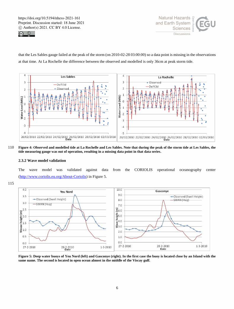
2.3.1 Storm tide validation

The hydrodynamic model was run from 20 February until 1 March 2010, the duration of the meteorological forcing data, with

GTSM astronomical tide boundary conditions. After 2 days of model spin-up, the comparison between the observed water

levels from SHOM tide gauges, and modelled water levels from Delft3d, during the whole simulation is good (Figure 4). Note 105


6

that the Les Sables gauge failed at the peak of the storm (on 2010-02-28 03:00:00) so a data point is missing in the observations

at that time. At La Rochelle the difference between the observed and modelled is only 36cm at peak storm tide.

Figure 4: Observed and modelled tide at La Rochelle and Les Sables. Note that during the peak of the storm tide at Les Sables, the 110 tide measuring gauge was out of operation, resulting in a missing data point in that data series.

2.3.2 Wave model validation

The wave model was validated against data from the CORIOLIS operational oceanography center

(http://www.coriolis.eu.org/About-Coriolis) in Figure 5.

115

Figure 5: Deep water buoys of Yeu Nord (left) and Gasconye (right). In the first case the buoy is located close by an Island with the

same name. The second is located in open ocean almost in the middle of the Viscay gulf.


7

2.4 Damage curves

Damage curves express the amount of damage experienced by a structure, relative to the structure’s total insured value. More 120

specifically, relates the cumulative distribution function, usually in terms of the standardized normal distribution function with

the damages (Suppasri et al., 2013; Sihombing and Torbol, 2016).

𝑃(𝑥) = Φ [𝑥−𝜇

𝜎] , (2)

where 𝑃(𝑥) is the cumulative probability of damage level 𝑥, Φ is the standardized normal distribution, 𝜇 is the median and 𝜎

the standard deviation (Tsubaki et al., 2016). It is also very common to express the previous equation as a logarithmic function 125

in order to obtain easily the parameters of the distribution with least square fitting as proposed by Suppasri et al., 2013. In the

present paper the parameters are assessed using the L-moments package within the open source program R. In this way it is

possible to relate different hydrodynamic variables with the damage ratio. From the 423 claims data within our domain,

approximately 185 are on Ille du Re, and the remaining 238 in the towns of La Rochelle, Aytré, Yves, Châtelaillon-Plage and

Fouras. 130

3 Results

After determining the model hydrodynamic and wave results (Figure 6) at the location of each claim location, the data were

subdivided into ten categories according to damage ratio level, and Box-Whisker plots were built to display the entire dataset

and analyse the trend of the data (Appendix A). Among the flow-only variables, the unit discharge (ℎ𝑣) appears to have the

clearest trend and least scatter. From the variables related to both flow and waves, the total force (𝐸𝑓

𝐶𝑔+ 𝜌ℎ𝑣2) appears to have 135

the clearest trend and correlation with the damage ratio. To better understand which of the variables fit Damage functions best,

three accuracy indicators are assessed: root mean square error (RMSE, Equation 3), Relative root square error (RRSE, Equation

4), and the Pearson correlation coefficient (ρ, Equation 5).

𝑅𝑀𝑆𝐸 = √∑ (𝑦′−𝑦)2𝑇

1

𝑇 , (3)

𝑅𝑅𝑆𝐸 = √∑ (𝑦′−𝑦)2𝑇

1

∑ (𝑦−�̅�)2𝑇1

, �̅� =∑ 𝑦𝑇

1

𝑇 (4) 140

𝜌𝑦,𝑦′ =

𝑐𝑜𝑣(𝑦,𝑦′)

𝜎𝑦𝜎𝑦′

, (5)

Where 𝑦′ is the predicted value, 𝑦 is the actual value and �̅� is the average of the actual values to predict, 𝑇 is the number of

values, and 𝜎 indicate the standard deviation


8

Figure 6: Maximum water level and maximum significant wave height footprints for the finer domain (case study area). water depth 145 and wave height are in units of m.

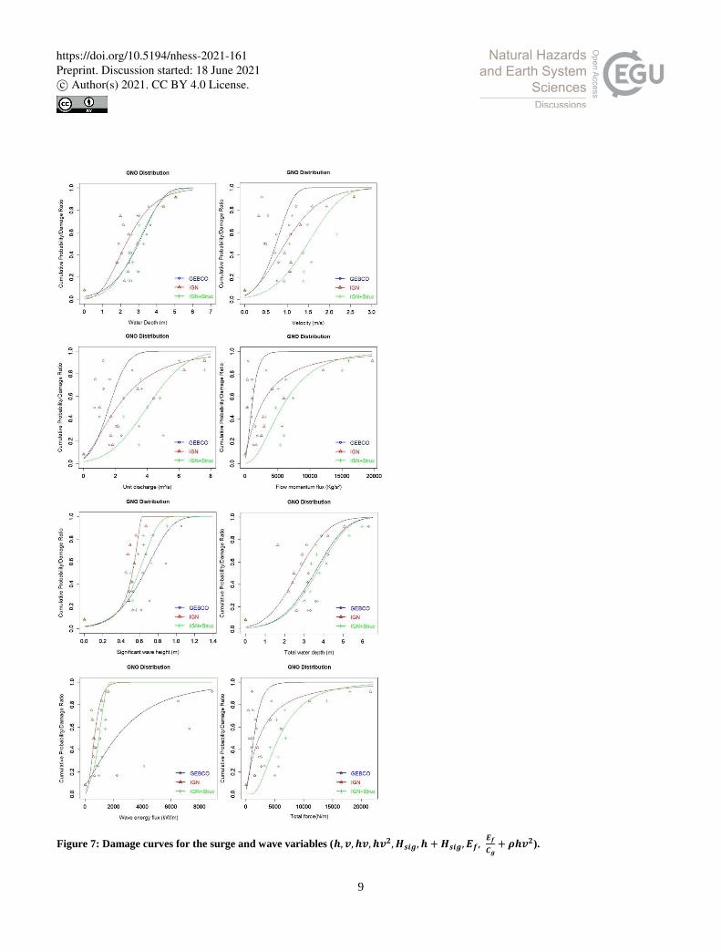
3.4 Damage curves from each digital elevation model

In order to build the damage curves with equation (2), the median values are extracted from the boxplots of appendix A (figures

A1 to A3) for each variable. In Figure 7 the damage curves for each hydrodynamic parameter are displayed in 3 lines, one for

each digital elevation model of Table 1. Similarly to Reese and Ramsay (2010), we find that greater than 90% of damage 150

occurs in the first 5m of flood depth.


9

Figure 7: Damage curves for the surge and wave variables (𝒉, 𝒗, 𝒉𝒗, 𝒉𝒗𝟐, 𝑯𝒔𝒊𝒈, 𝒉 + 𝑯𝒔𝒊𝒈, 𝑬𝒇,𝑬𝒇

𝑪𝒈+ 𝝆𝒉𝒗𝟐).


10

Table 2 shows that among the hydrodynamic parameters related only to storm surge, the water depth best fits Equation (2),

with the lowest errors (RMSE and RRSE) and the highest Pearson coefficient (ρ). In the same way, the variable that correlates 155

the best with the combined surge and wave parameters is the total (flow plus wave) force, using the IGN+Structures topography

and bathymetry (Table 1). This is related with the fact that this digital elevation model includes thin flood walls that contribute

to protection, and which can substantially modify the flow and wave fields over land.

Table 2: Goodness of fit for the flow only, and flow plus wave, parameters. The best fits for flow-only parameters are indicated in 160 green, and the best fits for flow plus wave parameters are indicated in blue.

Variable

𝑅𝑀𝑆𝐸 𝜌 𝑅𝑅𝑆𝐸

GEBCO IGN IGN +

Structures GEBCO IGN

IGN +

Structures GEBCO IGN

IGN +

Structures

Water depth (h) 0.1595 0.1898 0.1495 0.8134 0.7344 0.8328 0.1009 0.1145 0.0902

Flow speed (v) 0.3586 0.2561 0.2234 0.1284 0.5387 0.6406 0.2268 0.1545 0.1347

Unit discharge (ℎ𝑣) 0.3352 0.2272 0.2120 0.2421 0.6558 0.6744 0.2120 0.1370 0.1278

Flow momentum

flux (𝜌ℎ𝑣2) 0.3542 0.2540 0.1822 0.1314 0.5759 0.7622 0.2136 0.1532 0.1099

Significant wave

height (𝐻𝑠𝑖𝑔) 0.2211 0.2030 0.1600 0.6432 0.6901 0.8066 0.1398 0.1224 0.0965

Total water depth

(ℎ + 𝐻𝑠𝑖𝑔) 0.1767 0.2217 0.1522 0.7575 0.6404 0.8265 0.1117 0.1337 0.0918

Wave energy flux

(𝐸𝑓) 0.2649 0.2391 0.2307 0.5519 0.5851 0.6510 0.1676 0.1442 0.1391

Total force (𝐸𝑓

𝐶𝑔+

𝜌ℎ𝑣2)

0.3307 0.2494 0.1499 0.2396 0.5888 0.8387 0.2092 0.1504 0.0904

4 Discussion

The present paper considered the influence of flow-only variables (ℎ, 𝑣, ℎ𝑣, 𝜌ℎ𝑣2), and combined flow-wave parameters (ℎ𝑠𝑖𝑔,

ℎ + 𝐻𝑠𝑖𝑔, 𝐸𝑓,𝐸𝑓

𝐶𝑑+ 𝜌ℎ𝑣2). Flow depth and total (flow plus wave) force produce the best fits with analytical functions. 165

Goodness of fit to damage curves improve with quality of the topographic data used (Table 1). However, when applying

damage curves in practice, it is important to base predictions off a similar model setup to that used when calculating the damage

curves in the first place (Brussee et al., 2021). For example, if damage curves are built using coarse topography that neglects

the presence of thin seawalls (i.e. sheetpile/cantilever walls, or T- or L- walls), then the buildings protected by these walls

might experience more intense hydrodynamic conditions in the simulation than if the walls had been present in the simulation. 170

Since the actual recorded damage does not depend on the model used to calculate the hydrodynamic forcing conditions, damage


11

curves developed using the coarse resolution topography will be shifted to the right relative to damage curves generated with

the thin floodwalls present. If these damage curves generated using a coarse resolution simulation are then applied for damage

prediction by an external user who applies a high resolution simulation that resolves floodwalls, the reduced forcing (due to

the presence of these floodwalls) will generate a non-conservative result (too little damage), because the damage curves had 175

been generated using forcing data from a simulation where the floodwalls had not been present. Therefore, when damage

curves are reported in the literature, it is important to quantify how these vary with the topography used in the simulations on

which the damage curves are based. However, in the current paper, Figure 7 shows that damage curves do not vary consistently

leftward or rightward as topographic data are improved. This is because the response of forcing to the presence of these walls

is more complex than simply reducing wave height. If not overflowed, walls reduce damage greatly. However, water depth 180

can be exacerbated in front of walls, and flow can be channelled and intensified along walls, all increasing hydrodynamic

forcing in some locations, preventing a simple relation between topographic resolution and damage curve robustness.

In addition to the general sensitivity of damage curves to topographic data quality, the damage curves displayed in Figure 7

do not consider certain physical wave-driven phenomena such as wave overtopping of structures (Lashley et al., 2020a) or 185

infragravity waves generated by waves breaking in shallow water (Roeber and Bricker, 2015). For instance Lashley et al.

(2019) discussed the importance of dike overtopping due to infragravity waves on nearshore developments that can induce

wave-driven coastal inundation. The wave model used here, SWAN, does not include infragravity waves, nor does the

combined Delft3D/SWAN flow/wave model simulate wave overtopping of dikes, possibly leading to an underestimation of

the hydrodynamic forces on buildings, which would affect the resulting damage functions. However, consideration of wave 190

overtopping and infragravity effects requires either phase-resolving wave simulations or empirical relations specific to the

local topography (Lashley et al., 2020b), though this is beyond the scope of the current study, and is similarly neglected by

most other large-scale inundation studies (i.e., Sebastian et al, 2014; Kress et al., 2016: Kowaleski et al., 2020). Nonetheless,

the effect of infragravity oscillations and wave overtopping on resulting damage is an important item for future research.

5 Conclusions 195

Using insurance claims to build damage curves from the structures located in La Rochelle and surroundings provides valuable

information on the future damages that can be expected from an extratropical storm strike on the French Atlantic coast. In the

present study, the best correlation between the damage ratio and the hydrodynamic variables are the flow depth and the total

(flow plus wave) force for the aforementioned flow-only and flow-plus-wave variables respectively.

200

The uncertainty and variability within this methodology can be explained by two factors: 1) the hydrodynamic modelling, and

consequently, uncertainty in the hydrodynamic variables, and 2) uncertainty in the claims data. Regarding the first point, there

is a trend that indicates that better topography/bathymetry data gives hydrodynamic variables that correlate better with the


12

damage ratio. The explanation of this is basically because higher resolution data brings generally more accurate results of the

real flood conditions (Luppichini et al., 2019 and Ettritcha et al., 2018). Damage curves developed with a better representation 205

of the topography (IGN + structures) improve the accuracy indicators (Table 2), though scatter in the data itself (Figures A1,

A2 or A3) is large for all topographies. The second point, deals with the quality of the damage ratio data. It is well identified

that claims are subject to fraud and information distortion. Also variables related with the vulnerability of the assets like the

construction characteristics, the materials, the quality and the age of the structures (Paprotny et al., 2021) play an important

role in whether for a particular hydrodynamic variable value damage occurs or not. This adds a degree of complexity to the 210

analysis

In addition to the sensitivity of results to resolution of the topographic and bathymetric data, the inclusion of thin flood walls

via a land survey carried out by the authors also had a significant effect on the damage functions generated. This is important

to note, as thin steel or concrete structures like flood walls at typically only a few 10’s of centimetres thick, and so do not 215

appear in digital elevation models. The effect of these thin structures on the resulting damage functions shows the importance

of locally sourcing elevation data for the thin structures that are present, when conducting risk analyses for coastal regions,

though it is imperative to keep in mind agreement between the simulations used for developing the damage relations in the

first place, with those where the damage relations are applied for further risk analysis.

Acknowledgements 220

This work is funded by the AXA Joint Research Initiative (JRI) project INFRA: Integrated Flood Risk Assessment. A special

acknowledgement to Adri Mourits from Deltares for the help provided with the Delft3d debugging and Christopher Lashley

for the help during the field trip in Ille du Re and surrounding during August of 2020.

References

225

Bricker J., Esteban M., Takagi H., Roeber V., “Economic feasibility of tidal stream and wave power in post-Fukushima Japan”,

Renewable Energy, 114 pg32-45, 2017.

Brussee, A.R., Bricker, J.D., De Bruijn, K.M., Verhoeven, G.F., Winsemius, H.C. and Jonkman, S.N., Impact of hydraulic

model resolution and loss of life model modification on flood fatality risk estimation: Case study of the Bommelerwaard, The 230

Netherlands. Journal of Flood Risk Management, p.e12713, 2021.


13

Büttner O., “The influence of topographic and mesh resolution in 2D hydrodynamic modelling for floodplains and urban

areas”, EGU General Assembly Conference Abstracts, 2007.

235

De Risi R., Goda K., Yasuda T., Mori N., “Is flow velocity important in tsunami empirical fragility modeling?”, Earth-Science

Reviews, Volume 166, Pages 64-82, ISSN 0012-8252, 2017.

Deltares, “Delft3d user manual”, Version: 3.15, SVN Revision: 70333, 2021.

240

Chauveau E., Chadenas C., Comentale B., Pottier P., Blanlœil A., Feuillet T., Mercier D., Pourinet L., Rollo N, Tillier I. and

Trouillet B., Xynthia: lessons learned from a catastrophe, Environment, Nature and Landscape,

https://doi.org/10.4000/cybergeo.28032, 2011.

Englhardt J., de Moel H., Huyck C., de Ruiter M., Aerts J. and Ward P., “Enhancement of large-scale flood risk assessments 245

using building-material-based vulnerability curves for an object-based approach in urban and rural areas”, Natural Hazards

and Earth System Sciences, 2019.

Ettritcha G., Hardya A., Bojangb L., Crossc D., Buntinga P. and Brewera P ., “Enhancing digital elevation models for hydraulic

modelling using flood frequency detection”, Remote Sensing of Environment, 217, 506–522, 2018. 250

GEBCO, The General Bathymetric Chart of the Oceans, available at: https://www.gebco.net/, 2020.

Hatzikyriakou A. and Lin N., Assessing the Vulnerability of Structures and Residential Communities to Storm Surge: An

Analysis of Flood Impact during Hurricane Sandy, Front. Built Environ, 2018. 255

Huizinga, J., De Moel, H. and Szewczyk, W., Global flood depth-damage functions: Methodology and the database with

guidelines, EUR 28552 EN, Publications Office of the European Union, Luxembourg, ISBN 978-92-79-67781-6,

doi:10.2760/16510, JRC105688, 2017.

260

Jansen, L., Korswagen, P. A., Bricker, J. D., Pasterkamp, S., de Bruijn, K. M., & Jonkman, S. N., Experimental determination

of pressure coefficients for flood loading of walls of Dutch terraced houses. Engineering Structures, 216, 110647, 2020.

Kowaleski, A.M., Morss, R.E., Ahijevych, D. and Fossell, K.R., Using a WRF-ADCIRC ensemble and track clustering to

investigate storm surge hazards and inundation scenarios associated with Hurricane Irma. Weather and Forecasting, 35(4), 265

pp.1289-1315, 2020.


14

Kreibich H., Piroth K., Seifert I., Maiwald H., Kunert U., Schwarz J., Merz B. and Thieken A., “Is flow velocity a significant

parameter in flood damage modelling?”, Natural Hazards and Earth System Sciences, 2009.

270

Kress, M.E., Benimoff, A.I., Fritz, W.J., Thatcher, C.A., Blanton, B.O. and Dzedzits, E., Modeling and simulation of storm

surge on Staten Island to understand inundation mitigation strategies. Journal of Coastal Research, (76), pp.149-161, 2016.

Lashley C., Bertin X., Roelvink D. and Arnaud G., “Contribution of Infragravity Waves to Run-up and Overwash in the Pertuis

Breton Embayment (France)”, Journal of Marine Science and Engineering, 2019. 275

Lashley, C.H., Bricker, J.D., van der Meer, J., Altomare, C. and Suzuki, T., Relative magnitude of infragravity waves at coastal

dikes with shallow foreshores: a prediction tool. Journal of Waterway, Port, Coastal, and Ocean Engineering, 146(5),

p.04020034, 2020a.

280

Lashley, C.H., Zanuttigh, B., Bricker, J.D., van der Meer, J., Altomare, C., Suzuki, T., Roeber, V. and Oosterlo, P.,

Benchmarking of numerical models for wave overtopping at dikes with shallow mildly sloping foreshores: Accuracy versus

speed. Environmental Modelling & Software, 130, p.104740, 2020b.

Luppichini M., Favalli M., Isola I., Nannipieri L., Giannecchini R. and Bini M., “Influence of Topographic Resolution and 285

Accuracy on Hydraulic Channel Flow Simulations: Case Study of the Versilia River (Italy)”, Remote Sensing, 2019.

Muis S., Verlaan M., Winsemius H., Aerts J. and Ward P, “A global reanalysis of storm surges and extreme sea levels”, Nature

Communications 7, 11969, 2016.

290

Paprotny D., Kreibich H., Morales‑Nápoles O., Wagenaar D., Castellarin A., Carisi F., Bertin X., Merz B. and Schröter K.,

“A probabilistic approach to estimating residential losses from different flood types”, Natural Hazards 105:2569–2601, 2021.

Pistrika A., Jonkman S., “Damage to residential buildings due to flooding of New Orleans after hurricane Katrina”, Journal of

Natural Hazards. Vol. 54 pg; 413-434, 2010. 295

Postacchini M., Zitti G., Giordano E., Clementi F., Darvini G., Lenci S., “Flood impact on masonry buildings: The effect of

flow characteristics and incidence angle”, Journal of Fluids and Structures, Volume 88, 2019.


15

Pregnolato M., Galasso C. and Parisi F., “A Compendium of Existing Vulnerability and Fragility Relationships for Flood: 300

Preliminary Results”, 12th International Conference on Applications of Statistics and Probability in Civil Engineering, 2015.

Reese S. and Ramsay D., “RiskScape: Flood fragility methodology”, Technical Report: WLG2010-45, 2010.

Roeber, V. and Bricker, J.D.. Destructive tsunami-like wave generated by surf beat over a coral reef during Typhoon 305

Haiyan. Nature communications, 6(1), pp.1-9, 2015.

Sebastian, A., Proft, J., Dietrich, J.C., Du, W., Bedient, P.B. and Dawson, C.N., Characterizing hurricane storm surge behavior

in Galveston Bay using the SWAN+ ADCIRC model. Coastal Engineering, 88, pp.171-181, 2014.

310

Sihombing F. and Torbol M., “Analytical fragility curves of a structure subject to tsunami waves using smooth particle

hydrodynamics”, Smart Structures and Systems, 2016.

Slomp R., Kolen B., Bottema M. and Teun Terptsra, Learning from French Experiences with Storm Xynthia – Damages after

A Flood”, Learning from large flood events abroad, 2010. 315

Smith S., and Banke E.. “Variation of the sea surface drag coefficient with wind speed.” Quarterly Joournal of the Royal

Meteorological Society 101: 665–673, 1975.

Suppasri, A., Mas, E., Charvet, I., Gunasekera, R., Imai, K., Fukutani, Y., Abe, Y., Imamura, F., Building damage 320

characteristics based on surveyed data and fragility curves of the 2011 great east Japan tsunami. Nat. Hazards 66 (2), 319–341,

2013.

Tiggeloven T., de Moel H., Winsemius H., Eilander D., Erkens G., Gebremedhin E., Diaz-Loaiza A., Kuzma S., Luo T.,

Iceland C., Bouwman A., van Huijstee J., Ligtvoet W. and Ward P.,” Global-scale benefit–cost analysis of coastal flood 325

adaptation to different flood risk drivers using structural measures”, Natural Hazards and Earth System Sciences, 2020.

Tomiczek T., Kennedy A., Zhang Y., Owensby M., Hope M., Lin N., and Flory A., “Hurricane Damage Classification

Methodology and Fragility Functions Derived from Hurricane Sandy’s Effects in Coastal New Jersey”, Journal of Waterway

Port Coastal and Ocean Engineering, 2017. 330

Tsubaki R., Bricker J., Ichii K. and Kawahara Y., “Development of fragility curves for railway embankment and ballast scour

due to overtopping flood flow”, Natural Hazards and Earth System Sciences, 2016.


16

Appendix A

Whisker plots from which damage curves are developed are shown in Figures A1, A2, and A3. Digital Elevation Models are 335

as described in Table 1. The damage curves of Figure 7 use the median values (red lines) from each of the figures in this

appendix.

Figure A1: Box-Whisker plots for the variables (𝒉, 𝒗, 𝒉𝒗, 𝒉𝒗𝟐, 𝑯𝒔𝒊𝒈, 𝒉 + 𝑯𝒔𝒊𝒈, 𝑬𝒇,𝑬𝒇

𝑪𝒈+ 𝝆𝒉𝒗𝟐) with the GEBCO DEM.


17

340


𝑪𝒈+ 𝝆𝒉𝒗𝟐) with the IGN DEM.


18


𝑪𝒈+ 𝝆𝒉𝒗𝟐) with the IGN+Structures DEM.


Development of damage curves for buildings near La ...

Documents

Transcript of Development of damage curves for buildings near La ...