New Molecular Based Methods of Diagnosis DNA based molecular methods.

Development of Computer-Aided Molecular Design Methods for Bioengineering Applications
By
Brock C. Roughton
Submitted to the graduate degree program in Bioengineering and the Graduate Faculty of the
University of Kansas in partial fulfillment of the requirements for the degree of Doctor of
Philosophy.
________________________________
Chairperson Dr. Kyle Camarda
________________________________
Dr. Stevin Gehrke
________________________________
Dr. Luke Huan
________________________________
Dr. Sarah Kieweg
________________________________
Dr. Jennifer Laurence
Date Defended: December 9th
, 2013
ii
The Dissertation Committee for Brock C. Roughton
certifies that this is the approved version of the following dissertation:
Development of Computer-Aided Molecular Design Methods for Bioengineering Applications
________________________________
Chairperson Dr. Kyle Camarda
Date Approved: December 13th
, 2013
iii
ABSTRACT
Computer-aided molecular design (CAMD) offers a methodology for rational product design. The CAMD
procedure consists of pre-design, design and post-design phases. CAMD was used to address two
bioengineering problems: design of excipients for lyophilized protein formulations and design of ionic
liquids for use in bioseparations. Protein stability remains a major concern during protein drug
development. Lyophilization, or freeze-drying, is often sought to improve chemical stability. However,
lyophilization can result in protein aggregation. Excipients, or additives, are included to stabilize proteins
in lyophilized formulations. CAMD was used to rationally select or design excipients for lyophilized
protein formulations. The use of solvents to aid separation is common in chemical processes. Ionic
liquids offer a class of molecules with tunable properties that can be altered to find optimal solvents for
a given application. CAMD was used to design ionic liquids for extractive distillation and in situ extractive
fermentation processes.
The pre-design phase involves experimental data gathering and problem formulation. When available,
data was obtained from literature sources. For excipient design, data of percent protein monomer
remaining post-lyophilization was measured for a variety of protein-excipient combinations. In problem
formulation, the objective was to minimize the difference between the properties of the designed
molecule and the target property values. Problem formulations resulted in either mixed-integer linear
programs (MILPs) or mixed-integer non-linear programs (MINLPs).
The design phase consists of the forward problem and the reverse problem. In the forward problem,
linear quantitative structure-property relationships (QSPRs) were developed using connectivity indices.
Chiral connectivity indices were used for excipient property models to improve fit and incorporate
three-dimensional structural information. Descriptor selection methods were employed to find models
that minimized Mallow's Cp statistic, obtaining models with good fit while avoiding overfitting. Cross-
iv
validation was performed to access predictive capabilities. Model development was also performed to
develop group contribution models and non-linear QSPRs. A UNIFAC model was developed to predict
the thermodynamic properties of ionic liquids.
In the reverse problem of the design phase, molecules were proposed with optimal property values.
Deterministic methods were used to design ionic liquids entrainers for azeotropic distillation. Tabu
search, a stochastic optimization method, was applied to both ionic liquid and excipient design to
provide novel molecular candidates. Tabu search was also compared to a genetic algorithm for CAMD
applications. Tuning was performed using a test case to determine parameter values for both methods.
After tuning, both stochastic methods were used with design cases to provide optimal excipient
stabilizers for lyophilized protein formulations. Results suggested that the genetic algorithm provided a
faster time to solution while the tabu search provides quality solutions more consistently.
The post-design phase provides solution analysis and verification. Process simulation was used to
evaluate the energy requirements of azeotropic separations using designed ionic liquids. Results
demonstrated that less energy was required than processes using conventional entrainers or ionic
liquids that were not optimally designed. Molecular simulation was used to guide protein formulation
design and may prove to be a useful tool in post-design verification. Finally, prediction intervals were
used for properties predicted from linear QSPRs to quantify the prediction error in the CAMD solutions.
Overlapping prediction intervals indicate solutions with statistically similar property values. Prediction
interval analysis showed that tabu search returns many results with statistically similar property values
in the design of carbohydrate glass formers for lyophilized protein formulations. The best solutions from
tabu search and the genetic algorithm were shown to be statistically similar for all design cases
considered. Overall the CAMD method developed here provide a comprehensive framework for the
design of novel molecules for bioengineering approaches.

v
ACKNOWLEDGEMENTS
While only one name appears as author, my dissertation would not be possible without the help and
support of many different individuals. First and foremost, I would like to express my gratitude towards
God for providing perspective and direction in my life. I have been very blessed to have the experiences
that graduate school as provided me. My wife Mary has been a constant source of affirmation for me. I
thank her for being my partner throughout my years in graduate school despite any discomfort the
weird hours and extended absences may have caused her. I have enjoyed her constant company as I
journeyed from Colorado to Kansas, then Denmark, back to Kansas, to Indiana and a final return to
Kansas in pursuit of my degree. I also thank my son Charlie for being a part of nearly the last two years
of my graduate studies. He has brought a deeper meaning to my life and I enjoy spending every day with
him. I appreciate all that my dad Bryan, mom Marie, sister Jessica and brother-in-law Matt have done to
welcome us to the Sunflower State and the assistance they have offered us. I can't thank Mary's parents
Hilary and Robert and her siblings Samuel and Grace enough for welcoming me into their family. They
have provided continual support to Mary and I. Both Mary and my mom provided excellent editorial
advice while writing my dissertation, providing the outside eye that is sometimes necessary to catch the
most obvious mistakes.
My time in graduate school has exceeded my expectations and that is due in no small part to my advisor
Dr. Kyle Camarda. I appreciate all that he has done to progress my professional development. He has
provided me with numerous opportunities and allowed me the freedom to become confident in my own
abilities. Besides an advisor, I am glad to count Kyle as a true friend. I would like to thank my dissertation
committee for all that I have learned from them through courses and my comprehensive exam. Their
instruction has improved the work that follows. I appreciate the guidance that Dr. Liz Topp from Purdue
University has provided. She helped me to look at my work from a different perspective. I am especially

vi
grateful for her providing me the opportunity to spend a semester at Purdue learning the experimental
side of proteins. My education would be incomplete without the lessons I learned while in her lab.
I would like to extend a special thank you to all the members of the Camarda lab for their help and
support over the years. Thanks go to John Eslick and JR Hacker for proving that graduation is possible!
Thank you to Thora Whitmore, Rajib Anwar and Farhana Abedin for making my time in graduate school
better. My appreciation goes out to the members of the Topp lab that made me feel welcome at
Purdue: Lavanya Iyer, Saradha Chandrasekhar, Jainik Panchal, Bo Xie, Moorthy Balakrishnan and
Andreas Sophocleous. I would also like to acknowledge all the hard-working undergraduates that I have
had the pleasure to work with: Qi Chen, Haider Tarar, Briana Christian, John White, Anthony Pokphanh,
Taylor Wilson and Steele Reynolds. I have met many great people while at KU and am very grateful to all
the friends that I have made. You have all made my time here more worthwhile.

vii
CONTENTS Abstract ........................................................................................................................................................ iii
Acknowledgements ....................................................................................................................................... v
List of Figures ............................................................................................................................................... xi
List of Tables ...............................................................................................................................................xiii
1.0 Introduction ...................................................................................................................................... 1
1.1 Motivation ........................................................................................................................................... 2
1.2 Overview ............................................................................................................................................. 6
2.0 Background ....................................................................................................................................... 8
Lyophilized Protein Formulation Design ................................................................................................... 8
2.1 Proteins as Drugs ................................................................................................................................ 8
2.2 Lyophilization .................................................................................................................................... 11
2.3 Protein Aggregation – Mechanisms, Measurement and Prediction ................................................. 12
2.4 Approaches to Aggregation Minimization ........................................................................................ 18
2.5 Vitrification – Glass Transitions in Lyophilization ............................................................................. 23
2.6 Protein-Excipient Interactions in the Dried State ............................................................................. 27
Ionic Liquid Solvent Design ..................................................................................................................... 29
2.7 Use of Separation Media for Azeotropic Distillation and in situ Fermentation ................................ 29
2.8 Ionic Liquids as Separation Media .................................................................................................... 31
Forward Problem .................................................................................................................................... 33
2.9 Descriptors Used in Structure-Property Models ............................................................................... 33
2.10 Property Model Development ........................................................................................................ 35
2.11 Thermodynamic Property Modeling and Prediction ...................................................................... 37
Reverse Problem ..................................................................................................................................... 38
2.12 Computer-Aided Molecular Design (CAMD) Overview and Problem Formulation ........................ 38
2.13 Enumeration Solution Methods ...................................................................................................... 41
2.14 Deterministic Solution Methods ..................................................................................................... 42
2.15 Stochastic Solution Methods .......................................................................................................... 43
2.16 Integrated Product-Process Design ................................................................................................ 45
2.17 Post-Design Methods ...................................................................................................................... 46
3.0 Experimental Methods.................................................................................................................... 48

viii
3.1 Experimental Overview ..................................................................................................................... 48
3.1.1 Materials .................................................................................................................................... 49
3.1.2 Sample Preparation.................................................................................................................... 50
3.1.3 Lyophilization ............................................................................................................................. 51
3.2 Ultraviolet-Visible Light Spectrophotometry (UV-Vis) ...................................................................... 52
3.2.1 Theory ........................................................................................................................................ 52
3.2.2 Experimental Procedure ............................................................................................................ 54
3.3 Size-Exclusion Chromatography (SEC) .............................................................................................. 55
3.3.1 Theory ........................................................................................................................................ 55
3.3.2 Experimental Procedure ............................................................................................................ 57
3.4 Sodium-Dodecyl-Sulfate Polyacrylamide Gel Electrophoresis (SDS-PAGE) ...................................... 57
3.4.1 Theory ........................................................................................................................................ 57
3.4.2 Experimental Procedure ............................................................................................................ 58
3.5 Powder X-ray Diffraction (pxrd) ........................................................................................................ 59
3.5.1 Theory ........................................................................................................................................ 59
3.5.2 Experimental Procedure ............................................................................................................ 62
3.6 Hydrogen-Deuterium Exchange Mass Spectroscopy (HX-MS) .......................................................... 63
3.6.1 Theory ........................................................................................................................................ 63
3.6.2 Use in Lyophilized Solids ............................................................................................................ 65
4.0 Property Model Development: The Forward Problem ................................................................... 67
4.1 Calculation of Molecular Descriptors ................................................................................................ 70
4.1.1 Group Contribution .................................................................................................................... 70
4.1.2 Connectivity Indices ................................................................................................................... 71
4.1.3 Protein-Based Descriptors ......................................................................................................... 74
4.1.4 Principal Component Analysis .................................................................................................... 75
4.2 Development of Linear QSPRs .......................................................................................................... 76
4.2.1 Glass Transition Properties ........................................................................................................ 76
4.2.2 Percent Monomer Remaining Following Lyophilization ............................................................ 76
4.2.3 Properties for in situ NDHD recovery ........................................................................................ 77
4.2.4 Descriptor selection ................................................................................................................... 78
4.2.5 Cross-Validation ......................................................................................................................... 80
4.3 Development of Non-Linear QSPRs .................................................................................................. 81
ix
4.3.1 Selection of Functional Forms .................................................................................................... 81
4.3.2 Parameter Fitting ....................................................................................................................... 82
4.3.3 Parameter Sensitivity ................................................................................................................. 82
4.3.4 Statistical Verification ................................................................................................................ 83
4.4 Group Contribution Methods ........................................................................................................... 84
4.4.1 Hildebrand Solubility Parameter ................................................................................................ 84
4.4.2 Thermal Decomposition Temperature ...................................................................................... 86
4.4.3 Group Contribution Model Development .................................................................................. 86
4.5 UNIFAC-IL Model Development ........................................................................................................ 93
4.5.1 Theory ........................................................................................................................................ 93
4.5.2 Determination of Groups and Group Parameters ..................................................................... 96
4.5.3 Determination of Interaction Parameters ................................................................................. 97
5.0 Molecular Design Methods: The Reverse Problem ........................................................................ 98
5.1 Deterministic Design of Ionic Liquid Entrainers ................................................................................ 98
5.2 Use of Tabu Search in Design of Ionic Liquid Extractants and Carbohydrate Glass-Formers ......... 101
5.3 Development of Stochastic Design Methods for Carbohydrate Excipients in Lyophilized Protein
Formulations ......................................................................................................................................... 102
5.4 Tuning of Stochastic Design Methods for Carbohydrate Excipients in Lyophilized Protein
Formulations ......................................................................................................................................... 117
5.4.2 Genetic Algorithm .................................................................................................................... 119
5.5 Comparison of Stochastic Design Methods for Carbohydrate Excipients in Lyophilized Protein
Formulations ......................................................................................................................................... 119
6.0 Simultaneous Product and Process Design ................................................................................... 122
6.1 Driving Force Based Design ............................................................................................................. 123
6.2 Azeotrope Separation Process Simulation ...................................................................................... 125
7.0 Molecular Simulation for Design and Post-Design Stages ............................................................ 128
7.1 Use of AutoDock for Blind Docking Simulations ............................................................................. 129
7.2 Determination of Protein-Excipient Interactions ............................................................................ 129
7.3 Optimal Selection of Excipients ...................................................................................................... 130
7.4 Docking Simulation Results ............................................................................................................. 132
7.5 Formulation Selection for Maximizing Protein-Excipient Interactions ........................................... 134
8.0 Results for Ionic Liquid Design ...................................................................................................... 136

x
8.1 Hildebrand Solubility Parameter Group Contribution Model ......................................................... 136
8.2 UNIFAC-IL Model ............................................................................................................................. 138
8.3 CAMD Results for Ionic Liquid Entrainers ....................................................................................... 144
8.4 Design of Ionic Liquid-Based Azeotropic Separation Processes ..................................................... 149
8.5 Prediction of Relevant Properties for in situ Extractive Fermentation ........................................... 154
8.6 CAMD results for in situ Extractants ............................................................................................... 156
9.0 Results for Lyophilized Excipient Design ....................................................................................... 158
9.1 Glass Transition Temperature Property Models ............................................................................. 158
9.2 Results for Optimal Glass Former Design ....................................................................................... 163
9.3 Experimental Results for Post-Lyophilization Protein Loss ............................................................. 167
9.4 Post-Lyophilization Protein Loss Models: As a Function of Protein Structure................................ 170
9.5 Post-Lyophilization Protein Loss Models: As a Function of Excipient Structure ............................. 181
9.5.1 Principal Component Analysis and Descriptor Comparison .................................................... 182
9.5.2 Correlation and K-Fold Cross-Validation .................................................................................. 184
9.6 Post-Lyophilization Protein Loss Models: As a Function of Both Protein and Excipient Structure 190
9.7 Stochastic Optimization Tuning Results .......................................................................................... 195
9.8 Results for Optimal Design of Stabilizers for Lyophilized Protein Formulations ............................ 207
10.0 Conclusions and Future Recommendations ..................................................................................... 217
References ................................................................................................................................................ 221
A. Nomenclature ................................................................................................................................... 232
B. R Procedure For Model Development .............................................................................................. 236
C. Polymer Designer Procedure ............................................................................................................ 244
Ionic Liquid Groups Used in Polymer Designer ..................................................................................... 246
Excipient Groups Used in Polymer Designer ......................................................................................... 247
D. CAMD Excipient Designer Source Code ............................................................................................ 249
CAMD Module Code ............................................................................................................................. 249
Property Module Code .......................................................................................................................... 257
Connectivity Indices Calculator Code.................................................................................................... 264
Tabu Search Code ................................................................................................................................. 269
Genetic Algorithm Code ........................................................................................................................ 276
E. UNIFAC-IL Interaction Parameters .................................................................................................... 282
F. Summary of Experimental Data ........................................................................................................ 285

xi
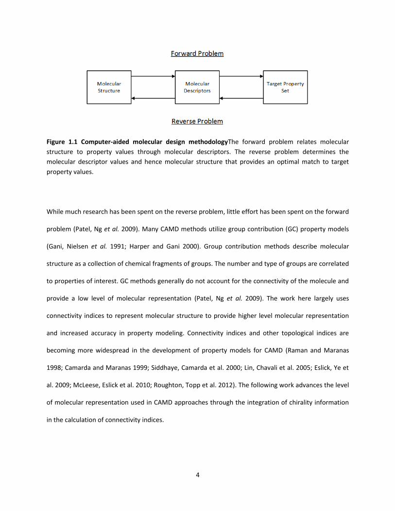
LIST OF FIGURES Figure 1.1 Computer-aided molecular design methodology ........................................................................ 4
Figure 2.1 Hierarchy of protein structure ................................................................................................... 10
Figure 2.2 Vial containing lyophilized protein formulation ........................................................................ 11
Figure 2.3 Solutions containing aggregated protein ................................................................................... 13
Figure 2.4 Pathway for the formation of aggregates through conformation instability ............................ 14
Figure 2.5 Preformulation and formulation development process diagram .............................................. 22
Figure 2.6 The phase transitions that occur during the lyophilization process .......................................... 26
Figure 2.7 Hydroxyl groups on sucrose ....................................................................................................... 28
Figure 2.8 Block flow diagram of azeotropic distillation process ............................................................... 30
Figure 2.9 Block flow diagram of in situ extractive fermentation .............................................................. 31
Figure 2.10 The ionic liquid 1,3-dimethylimidazolium dimethylphosphate (MMIm DMP) ........................ 32
Figure 2.11 A general procedure for the solution of the CAMD reverse problem ..................................... 39
Figure 2.12 Overview of integrated product and process design ............................................................... 46
Figure 3.1 Overview of experimental procedure used by author............................................................... 49
Figure 3.2 Chromophores commonly present in proteins .......................................................................... 53
Figure 3.3 Typical UV-Vis spectra for a protein .......................................................................................... 54
Figure 3.4 Overview of size-exclusion chromatography (SEC) .................................................................... 56
Figure 3.5 Representative gel following SDS-PAGE .................................................................................... 58
Figure 3.6 Diagram of typical powder x-ray diffraction setup .................................................................... 60
Figure 3.7 Representative x-ray diffraction patterns .................................................................................. 62
Figure 3.8 A peptide bond, which forms between amino acids to construct the protein backbone ......... 63
Figure 3.9 General experimental procedure for HX-MS experiments performed in aqueous solution ..... 65
Figure 4.1 Procedure for experimental data acquisition and model development for rational lyophilized
formulation development ........................................................................................................................... 68
Figure 4.2 Example group contributions for (A) ethanol, (B) acetone and (C) benzene ............................ 70
Figure 4.3 Comparison of the chiral structures of stereoisomers (A) glucose and (B) mannose ............... 73
Figure 4.4 Oxidation of naphthalene to (1R,2S)-1,2-naphthalene dihydrodiol (NDHD) ............................. 77
Figure 4.5 Values for Mallow’s Cp statistic versus model size (number of connectivity indices used) ...... 79
Figure 5.1 CAMD framework developed to design carbohydrate excipients using either tabu search or a
genetic algorithm ...................................................................................................................................... 103
Figure 5.2 Number of possible combinations of groups that would provide solutions to a CAMD problem
.................................................................................................................................................................. 106
Figure 5.3 Tabu search algorithm as implemented in the CAMD framework .......................................... 111
Figure 5.4 Genetic algorithm as implemented in the CAMD framework ................................................. 115
Figure 6.1 Overall methodology for simultaneous design of ionic liquid entrainers and IL-based
separation processes ................................................................................................................................ 122
xii
Figure 6.2 Proposed ionic liquid-based azeotropic separation process ................................................... 125
Figure 7.1 Frequency of amino acid residues of calmodulin in contact with trehalose ........................... 133
Figure 7.2 Trehalose interaction regions mapped to the surface of calmodulin ..................................... 133
Figure 8.1 Comparison between experimental and predicted solubility parameter values .................... 137
Figure 8.2 Acetone-methanol-[emim][triflate] x-y diagram at 100 kPa ................................................... 141
Figure 8.3 1-propanol-water-[emim][triflate] x-y diagram at 100 kPa ..................................................... 141
Figure 8.4 Ethyl acetate-ethanol-[emim][triflate] x-y diagram at 100 kPa ............................................... 142
Figure 8.5 Ethanol-water-[emim][triflate] x-y diagram at 100 kPa .......................................................... 142
Figure 8.6 1-propanol-water-[mmim][dmp] P-T diagram ......................................................................... 143
Figure 8.7 2-propanol- water-[mmim][dmp] P-T diagram ........................................................................ 143
Figure 8.8 x-y diagram showing the performance of several ionic liquid entrainers on the acetone-
methanol azeotrope at 101.325 kPa ......................................................................................................... 146
Figure 8.9 x-y diagram showing the performance of several ionic liquid entrainers on the ethanol-water
azeotrope at 101.325 kPa ......................................................................................................................... 147
Figure 8.10 Reboiler heat duty as a function of feed stage location for separation of the ethanol-water
azeotrope using various amounts of [mmim][dmp] as an entrainer........................................................ 150
Figure 8.11 Reboiler heat duty as a function of ionic liquid flow rate for separation of the ethanol-water
azeotrope using [mmim][dmp] as an entrainer ........................................................................................ 150
Figure 8.12 1-octyl-4-methylpyridinium trifluoromethane sulfonate ([ompy][triflate]) .......................... 153
Figure 8.13 1,3-dimethylimidazolium dimethylphosphate ([mmim][dmp]) ............................................. 153
Figure 8.14 Comparison of correlation coefficient values belong to different model sizes for the partition
coefficient model (Kx) ................................................................................................................................ 155
Figure 8.15 The best cation candidates for the design cases (A) and (B) ................................................. 156
Figure 9.1 Comparison of measured experimental values to QSPR predicted values for the glass
transition temperature of the anhydrous solute (Tg) ............................................................................... 160
Figure 9.2 Comparison of measured experimental values to QSPR predicted values for the glass
transition temperature of the maximally freeze-concentrated solute (Tg’) ............................................. 161
Figure 9.3 Comparison of measured experimental values to QSPR predicted values for the melting point
of ice (Tm’) ................................................................................................................................................. 162
Figure 9.4 Comparison of measured experimental values to QSPR predicted values for the Gordon-Taylor
constant (k) ............................................................................................................................................... 163
Figure 9.5 Optimal carbohydrate excipient candidate 1 proposed by CAMD using tabu search ............. 165
Figure 9.6 Optimal carbohydrate excipient candidate 2 proposed by CAMD using tabu search ............. 165
Figure 9.7 Optimal carbohydrate excipient candidate 3 proposed by CAMD using tabu serach ............. 166
Figure 9.8 Parity plots of experimental percent monomeric protein values (%Monomer) from SEC versus
predicted %Monomer values .................................................................................................................... 177
Figure 9.9 Principal component analysis of descriptor space for excipients used in study ..................... 182
Figure 9.10 Comparison of chiral and simple connectivity indices for BSA and RNAse carbohydrate
models ....................................................................................................................................................... 183
Figure 9.11 Parity plots of percent monomer remaining after lyophilization as a function of carbohydrate
excipient choice for (A) BSA, (B) RNAse A, (C) -Amylase, (D) Ovalbumin and (E) Trypsin Inhibitor ....... 185

xiii
Figure 9.12 Parity plots of percent monomer remaining after lyophilization as a function of amino acid
excipient choice for (A) BSA and (B) RNAse A ........................................................................................... 186
Figure 9.13 Parity plots of percent monomer remaining after lyophilization as a function of both protein
and excipient structure ............................................................................................................................. 193
Figure 9.14 Tuning results for tabu search with varying maximum number of non-improving iterations
.................................................................................................................................................................. 196
Figure 9.15 Tuning results for tabu search with varying maximum number of neighbors considered at
each iteration ............................................................................................................................................ 197
Figure 9.16 Tuning results for tabu search with varying tabu list length of stored solution .................... 198
Figure 9.17 Tuning results for tabu search with varying tabu criteria ...................................................... 199
Figure 9.18 Tuning results for genetic algorithm with varying maximum number of generations .......... 201
Figure 9.19 Tuning results for genetic algorithm with population size per generation ........................... 202
Figure 9.20 Tuning results for genetic algorithm with varying maximum probability that a member will
be selected as a parent ............................................................................................................................. 203
Figure 9.21 Comparison between objective function values obtained for all 100 trial solutions of the test
case by (A) tabu search and (B) the genetic algorithm ............................................................................. 205
Figure 9.22 Comparison between times to solution observed for all 100 trial solutions of the test case
during (A) tabu search and (B) the genetic algorithm .............................................................................. 206
Figure 9.23 Optimal carbohydrate stabilizer candidates for BSA, as determined by (A) tabu search and (B)
genetic algorithm ...................................................................................................................................... 209
Figure 9.24 Optimal carbohydrate stabilizer candidates for RNAse A, as determined by (A) tabu search
and (B) genetic algorithm ......................................................................................................................... 210
Figure 9.25 Optimal carbohydrate stabilizer candidates for -amylase, as determined by (A) tabu search
and (B) genetic algorithm ......................................................................................................................... 211
Figure 9.26 Optimal carbohydrate stabilizer candidates for ovalbumin, as determined by (A) tabu search
and (B) genetic algorithm ......................................................................................................................... 212
Figure 9.27 Optimal carbohydrate stabilizer candidates for trypsin inhibitor, as determined by (A) tabu
search and (B) genetic algorithm .............................................................................................................. 213
Figure 9.28 Comparison across protein models of average chemical information for solutions derived by
both tabu search and genetic algorithm ................................................................................................... 215
Figure F.1 Pxrd results for subset of formulations selected ..................................................................... 287
LIST OF TABLES Table 2.1 Summary of experimental techniques commonly utilized in the detection of protein aggregates
.................................................................................................................................................................... 16
Table 2.2 Common protein engineering targets for property improvement ............................................. 20
Table 2.3 Overview of stochastic approaches commonly used in CAMD ................................................... 44
Table 3.1 Biophysical descriptors for the proteins considered .................................................................. 50
Table 4.1 Summary of property models developed for both lyophilized protein formulation design and
ionic liquid design for use in separations of bio-products .......................................................................... 69

xiv
Table 4.2 Biophysical descriptors for the proteins considered .................................................................. 74
Table 4.3 Descriptors obtained and derived from aggregation propensity prediction methods ............... 75
Table 4.4 Ionic liquid groups used for GC model development .................................................................. 87
Table 5.1 Property targets for molecular design using tabu search ......................................................... 101
Table 5.2 Building block groups and chiral subgroups available for design of new excipient candidates 104
Table 5.3 Description of VBA functions and subroutines used for molecular representation ................. 108
Table 5.4 Moves used to generate neighbors to current solution in tabu search ................................... 112
Table 5.5 Moves used to generate offspring to selected parents in the genetic algorithm .................... 116
Table 5.6 Parameter values used for the base case during tuning of the tabu search ............................ 118
Table 5.7 Parameter values used for the base case during tuning of the genetic algorithm ................... 119
Table 6.1 Fixed parameters and free variables for ionic liquid-based extractive distillation processes .. 127
Table 7.1 Sugar-surfactant formulations selected for maximum interaction with hot spot regions ....... 134
Table 8.1 Group contribution values for ionic liquid Hildebrand solubility parameter model................. 138
Table 8.2 Volume (Rk) and surface area (Qk) parameters for the UNIFAC-IL model ................................. 139
Table 8.3 UNIFAC-IL binary interaction parameters for the groups used for the final design candidates in
the acetone-methanol and ethanol-water examples ............................................................................... 140
Table 8.4 Comparison of minimum amount of designed and experimentally selected ionic liquids
required to break the acetone-methanol and ethanol-water azeotropes at 101.325 kPa ...................... 148
Table 8.5 Simulation results for ionic liquid-based azeotropic separation processes .............................. 151
Table 9.1 Summary of glass transition-related QSPRs developed ............................................................ 159
Table 9.2 Property values of candidate carbohydrate excipients designed using tabu search ................ 164
Table 9.3 Descriptors selected using an exhaustive search method with model size selected by
minimizing Cp score ................................................................................................................................... 171
Table 9.4 Correlation results for all four formulations ............................................................................. 173
Table 9.5 Descriptors selected using a forward search method with AIC evaluation .............................. 174
Table 9.6 Summary of covariance analysis ............................................................................................... 179
Table 9.7 Comparison of model size (including intercept), R2 and Q2 values for final protein-specific
models selected ........................................................................................................................................ 187
Table 9.8 Protein-by-protein model parameters determined by multiple linear regression following
descriptor selection .................................................................................................................................. 189
Table 9.9 List of descriptors considered for non-linear model development .......................................... 191
Table 9.10 Summary statistics of non-protein specific model .................................................................. 192
Table 9.11 Final tuned values for tabu search and the genetic algorithm ............................................... 204
Table E.1 UNIFAC-IL group interaction parameters .................................................................................. 283
Table F.1 Summary of experimental measures of protein aggregation via SEC (% monomer), UV- Vis (AI)
and SDS-PAGE ........................................................................................................................................... 286
Table F.2 Experimental SEC results ........................................................................................................... 291
Table F.3 SDS-PAGE Results under non-reducing and reducing conditions ............................................. 292

1
1.0 INTRODUCTION
Chemical product design is an important, yet often overlooked, aspect of chemical engineering.
Traditionally, chemical engineering has focused on process design, yet the aim of any process is to
manufacture a product of value. The objective of process design is to maximize output and profit while
minimizing material and energy inputs. Additional factors, such as safety and environmental concerns,
further constrain the process design. The same design principles can be applied to chemical product
design, where a molecule requires specific chemical or physical properties for a certain task. Other
properties can be used as constraints to further ensure the designed product works to the correct
specifications. Chemical product design has been defined as the process in which needs are determined,
candidates are generated to meet needs, screening and selection of candidates identifies the best
candidate and the final candidate is manufactured into a finished product (Cussler and Moggridge 2011).
The product design problem is often addressed by extensive experimental generate-and-test
approaches. Such approaches would not be feasible in many process design problems, and thus systems
engineering and process design developed to identify solutions from a modeling, simulation and
optimization perspective. Computer-aided molecular design (CAMD) offers a methodology that aims to
reduce trial-and-error and rationally design and select candidates in chemical product design using
systems engineering principles. In general, CAMD aims to solve the chemical product design problem by
determining a molecule or formulation (mixture of molecules) that best matches a set of target
properties given an assortment of chemical groups (Gani 2004). The advent of engineering approaches
to biological systems presents many new opportunities for the application and further development of
computer-aided molecular design. The work that follows describes the development and use of CAMD
approaches towards two applications of biological relevance: design of lyophilized protein formulations
and design of ionic liquid solvents for use in separation of bio-products.
2
1.1 MOTIVATION
Protein drugs are a fast growing pharmaceutical market. Global spending on biologics, which include
protein drugs and cell-based therapies, in 2011 was $157Bn and is expected to grow to $200Bn by 2016
(source: IMS Health, http://www.imshealth.com). In relation to traditional pharmaceutical molecules,
biologics are gaining market share. Of the top 100 drugs by U.S. sales in the fourth quarter of 2012, 28
were protein drugs or other biologics (source: IMS Health, http://www.imshealth.com ). Lyophilization,
or freeze-drying, is a common process used to increase the stability of protein drug products through
the removal of water. Despite improvements to chemical stability, lyophilization can induce protein
aggregation. Protein aggregation is undesirable in drug products as it can reduce efficacy, cause
immunogenicity and/or result in product losses during production. Thus, reduction of protein
aggregation is a topic of extreme interest and concern in the pharmaceutical industry. The two general
approaches taken to minimize aggregation are protein engineering and formulation development. The
work detailed here focuses on use of CAMD for the design of a molecule or set of molecules for inclusion
in a lyophilized formulation with the aim of minimizing aggregation.
Another class of molecules receiving increased attention both in research and industry is ionic liquids.
The number of publications concerning ionic liquids has jumped from less than 100 in 2000 to nearly
2,500 in 2011 (Ann, Nicholas et al. 2012). Ionic liquids are attractive as environmentally friendly, or
“green”, solvents due to their extremely low vapor pressure and tunable properties through alteration
of the cation and anion selected (Marsh, Boxall et al. 2004; Zhao, Xia et al. 2005). Two bio-based
applications of ionic liquids as solvents are used as the basis for CAMD in this work: ionic liquids as
entrainers in azeotropic distillation and ionic liquids as extraction media for in situ fermentation
processes.
3
Distillation is a commonly used unit operation that allows for separation of products based on
differences in volatility. Azeotropic distillation allows separation of azeotropes through use of an
entrainer, further increasing the applications of distillation. A major drawback to distillation is the
energy requirements. Distillation processes are estimated to account for 40% of the entire energy usage
of the chemical processing industry in North America (U.S. Dept. of Energy 2001). The use of ionic liquids
as entrainers has shown improvements in energy requirements in comparison to conventional
entrainers used in azeotropic distillation (Seiler, Jork et al. 2004).
Fermentation is a common method which utilizes microorganisms for the production of chemicals.
Substrate/product inhibition and separation of chemical products are two main concerns that reduce
the efficiency of fermentation processes. By removing the product as it is produced, in situ fermentation
offers a solution to these concerns. Ionic liquids have been proposed for use as extractive media for in
situ fermentation processes due to their flexible properties obtained by altering the cation and anion
used (Gangu, Weatherley et al. 2009). Through CAMD methods, optimal ionic liquids can be identified
for azeotropic distillation and in situ fermentation resulting in increasingly efficient separation
processes.
CAMD provides a methodology for the rational design or selection of molecules for a specific task.
CAMD methodology consists of a forward and a reverse problem (Venkatasubramanian, Chan et al.
1994). In the forward problem, property models are developed which relate chemical structure to
properties of interest. The reverse problem determines a molecular structure which best matches a set
of target property values and property constraints. The overall design methodology is outlined by Figure
1.1.
4
Figure 1.1 Computer-aided molecular design methodologyThe forward problem relates molecular
structure to property values through molecular descriptors. The reverse problem determines the
molecular descriptor values and hence molecular structure that provides an optimal match to target
property values.
While much research has been spent on the reverse problem, little effort has been spent on the forward
problem (Patel, Ng et al. 2009). Many CAMD methods utilize group contribution (GC) property models
(Gani, Nielsen et al. 1991; Harper and Gani 2000). Group contribution methods describe molecular
structure as a collection of chemical fragments of groups. The number and type of groups are correlated
to properties of interest. GC methods generally do not account for the connectivity of the molecule and
provide a low level of molecular representation (Patel, Ng et al. 2009). The work here largely uses
connectivity indices to represent molecular structure to provide higher level molecular representation
and increased accuracy in property modeling. Connectivity indices and other topological indices are
becoming more widespread in the development of property models for CAMD (Raman and Maranas
1998; Camarda and Maranas 1999; Siddhaye, Camarda et al. 2000; Lin, Chavali et al. 2005; Eslick, Ye et
al. 2009; McLeese, Eslick et al. 2010; Roughton, Topp et al. 2012). The following work advances the level
of molecular representation used in CAMD approaches through the integration of chirality information
in the calculation of connectivity indices.

5
Descriptor selection is trivial in the development of GC property models as the descriptors needed are
defined by the types of chemical groups present in the model building set. GC models run the risk of
over-fitting as a result, potentially leading to poor property prediction. By using connectivity indices,
descriptor selection techniques become available to ensure the development of models with good fits
and predictive ability. The work here integrates established statistical techniques for descriptor selection
with CAMD model development for the first time. Additionally, model cross-validation methods used
previously in CAMD (Eslick, Ye et al. 2009) are further advanced.
Given a set of predictive property models, a CAMD solution technique is employed to design or select
candidate molecules for a given task in the reverse problem. Three main solution approaches have been
used in CAMD: enumeration techniques, mathematical programming and stochastic optimization (Eljack
and Eden 2008). Enumeration techniques use a set of chemical groups to generate all chemical
combinations and then screen the combinations using property targets and constraints. As the number
of groups and/or the maximum allowable molecule size becomes large, enumeration techniques can
suffer from combinatorial explosion. Enumeration approaches are also reliant on a predefined chemical
group set that may preclude the consideration of many novel molecules. Mathematical programming
poses the CAMD problem as a mixed integer linear program (MILP) or mixed integer nonlinear program
(MINLP). While solution of a MILP ensures that a globally optimal solution is found, many CAMD
problems require a MINLP representation. Solution of a MINLP can be computationally expensive and
does not guarantee that the solution found is the global optimum (Eljack and Eden 2008). Furthermore,
a global optimum may not be necessary or even meaningful for CAMD approaches due to uncertainties
in property prediction. CAMD methods which employ stochastic optimization algorithms are iterative
procedures which aim to find multiple near-optimal or locally optimal solutions. The speed in generation
of a set of many good candidate molecules makes stochastic optimization approaches attractive for
CAMD and stochastic approaches are the focus of this work. Genetic algorithm CAMD approaches mimic

6
evolution to refine a population of candidate molecules through a series of generations, until candidates
are identified that provide the best match to a set of target properties (Venkatasubramanian, Chan et al.
1994). Tabu search CAMD approaches use a local search to identify candidate molecules while
maintaining a history of previous solutions (Lin, Chavali et al. 2005). The solution history, stored in tabu
lists, is used to guide the local search and determine when the search should be expanded to consider
other, more diverse molecular structures (Lin, Chavali et al. 2005). While both methods have
advantages – multiple initial solutions (seed population) in genetic algorithms and memory guided
search (via tabu lists) in tabu search – the utility of one stochastic method over another for CAMD is not
established. The work that follows details the development, tuning and comparison of genetic
algorithms and Tabu search for CAMD to identify the strengths and weaknesses in both approaches.
Finally, as stochastic methods generate many locally optimal solutions, a comparison method would
provide a tool to determine the best subset of solutions for further consideration. The work here
demonstrates a novel application of prediction intervals to provide statistical comparisons of CAMD
solutions obtained from stochastic solution methods. The prediction interval comparisons are made
between solutions found using the same method and also between the best solutions found using
different methods.
1.2 OVERVIEW
The following chapter (Section 2) will offer further background into both the lyophilized protein
formulation and ionic liquid solvent design problems being considered, along with a detailed
explanation of CAMD methodology and state-of-the-art. In addition to the use of CAMD towards novel
applications, the work concerned here also presents new approaches for CAMD model development,
solution and final candidate selection. To design a molecule with target properties, models must exist
for prediction of the targeted properties. Experimental data is needed for model development. The

7
experimental methods used in the work are detailed in Section 3. Development of reliable property
models is imperative as the validity of a CAMD solution rests on the predicted properties being accurate.
The work described in Section 4 details the efforts made to improve property prediction by uniting
established statistical techniques to model development for CAMD problems. Solution of the CAMD
problem provides candidate molecules for a given application. The CAMD solution approaches
presented here are based on optimization frameworks and are detailed in Section 5. Solution of the
optimization problems are approached through both deterministic and stochastic methods, with the use
of stochastic methods being emphasized. Additional computational tools have been utilized and are
detailed in Section 6 (process design) and Section 7 (molecular simulation). Results are presented in
Section 8 (ionic liquid design) and Section 9 (excipient design). Finally, conclusions and future
recommendations are given in Section 10.
For further clarification, nomenclature is given in Appendix A. The procedure used for model
development is provided in Appendix B. Appendix C provides guidelines for using a previously existing
CAMD framework while Appendix D provides the source code for a new CAMD framework proposed
here. Additional interaction parameters for a UNIFAC model developed by this work are available in
Appendix E. All experimental data obtained by the author are summarized in Appendix F.
8
2.0 BACKGROUND
CAMD requires a product design problem for solution. Two different problems related to bioengineering
have been addressed here: design of lyophilized protein formulations to minimize aggregation and
design of ionic liquids for separation of bio-products. Background on lyophilization and protein
aggregation is given in Sections 2.1-2.6. Background regarding ionic liquids and their use in separations
is given in Sections 2.7-2.8. Once a design problem of interest has been identified, property models are
needed to link key properties for design to molecular structure (the forward problem). Sections 2.9-2.11
describe model development for both structure-property relationships as well as thermodynamic
property models. Upon creation of reliable property models, CAMD is used to generate candidates that
optimally match a given set of target properties (the reverse problem). The CAMD methodology and its
historical development are detailed in Sections 2.12-2.17.
LYOPHILIZED PROTEIN FORMULATION DESIGN
2.1 PROTEINS AS DRUGS
Proteins are increasingly being considered as therapeutic candidates. Proteins fulfill a multitude of
biological functions including catalysis, transport and structural support and consequently have been
indicated in numerous disease states (Leader, Baca et al. 2008). Currently, approved protein drugs are
available for treatment of a wide range of diseases including diabetes, multiple sclerosis, rheumatoid
arthritis, cancer and hepatitis (Marshall, Lazar et al. 2003). Compared to traditional small molecule
pharmaceuticals, protein molecules have increased complexity.
Proteins are biopolymers comprised of amino acids. The main structure of an amino acid involves an
amino group and carbonyl group common to all amino acids along with a side group that defines the
amino acid. There are twenty common amino acids used in the biosynthesis of proteins, which can be
arranged in classes of non-polar or hydrophobic, polar, acidic and basic amino acids. Two amino acids

9
bond covalently to form a peptide bond between the amide nitrogen of one amino acid and carbonyl
carbon of another amino acid. The formation of peptide bonds creates the polypeptide backbone which
is common among all proteins with structural diversity arising from the amino acid side groups. The
amino acid sequence of the protein is referred to as the primary structure. Proteins do not exist as linear
molecules but instead fold into a variety of three-dimensional conformations. Structural motifs known
as -helices and -sheets (pleated sheets) form the secondary structure of a protein. Such motifs are
formed by hydrogen bonding between the amide hydrogen of one amino acid and the carbonyl oxygen
of another amino acid. The three-dimensional arrangement of secondary structural elements and
unfolded regions constitutes the tertiary structure of the protein, which is driven by the amino acid
sequence (Anfinsen 1972). Minimization of exposed non-polar or hydrophobic surface area and
formation of intramolecular contacts are two main driving forces in the tertiary structure adopted by a
protein (Pace, Shirley et al. 1996; Rose, Fleming et al. 2006). Quaternary structure is derived from
arrangement of single folded polypeptide chains into multi-protein complexes. An overview of the
structural hierarchy in proteins is given by Figure 2.1. The biological function of proteins is derived from
protein structure. As a result, preservation of native structure is essential for proper function of
therapeutic proteins.

10
Figure 2.1 Hierarchy of protein structure Figure adapted from (University of Massachusetts, accessed 1 June 2013).
When a protein is identified as a therapeutic candidate, a formulation must be developed for
administration. Due to degradation processes in the body, protein drug products generally require
injectable routes of administration (intravenous, intramuscular or subcutaneous). Thus the final product
requires an injectable solution for patient use. Additives, or excipients, are included in the formulation
to attain desirable properties, including stabilization of the final drug product. Stability is a major
concern, as many degradation routes exist for proteins. For example, degradation can occur via
aggregation, deamidation, isomerization, oxidation, glycation, and thioldisulphide exchange (Cleland,
Langer et al. 1994; Manning, Chou et al. 2010). Degradation not only results in product loss, but also can
lead to issues in regulatory approval. In most cases, the FDA requires pharmaceutical product
degradation to be below 10% of the product’s final weight (Cleland, Langer et al. 1994).

11
2.2 LYOPHILIZATION
For proteins that prove unstable under aqueous conditions, lyophilization is often employed.
Lyophilization removes water from the formulation by sublimation via a freezing step and then by
evaporation through primary and secondary drying steps (Cleland, Langer et al. 1994; Costantino and
Pikal 2004). During the lyophilization process, the protein experiences several temperature and pressure
changes. By removing water, the mobility of the protein is reduced and stability is improved by
elimination of many reactions that are facilitated by water. The desired resulting product is an
amorphous solid with minimal water content (see Figure 2.2). Lyophilization is among the most common
formulation choices for protein drugs, representing 46% of the biopharmaceuticals approved by the FDA
through December 2003 (Costantino and Pikal 2004). For administration, lyophilized protein drug
products are reconstituted and subsequently injected.
Figure 2.2 Vial containing lyophilized protein formulation The resulting formulation is an amorphous
solid.
Despite improvements to stability, degradation can still occur in lyophilized proteins. Of particular
interest here is degradation due to protein aggregation, which is an often irreversible self-association
12
resulting in a protein complex (Cleland, Langer et al. 1994; Wang 2005; Wang, Nema et al. 2010). The
aggregation process can occur due to physical interactions between protein surfaces or can result from
chemical interactions of the amino acids, forming covalent bonds between proteins (Wang 2005). The
detection of aggregates is difficult, as the protein complexes may be soluble (Wang 2005). Aggregation
not only results in product loss and lowered efficacy of the protein drug, but can also lead to severe and
life threatening immunogenic responses (Rosenberg 2006). One aim of a lyophilized formulation should
be to minimize aggregation, ensuring the safety and efficacy of the final product.
2.3 PROTEIN AGGREGATION – MECHANISMS, MEASUREMENT AND PREDICTION
Protein aggregation is defined as the self-association of monomeric protein leading to the formation of
multi-protein complexes. Aggregation can be either reversible or irreversible, arising from the formation
of covalent bonds or through physical interactions (Wang 2005). An example of chemical reaction
leading to aggregation is the formation of intermolecular disulfide bonds. Interactions between
hydrophobic regions of proteins represent a physical pathway that results in aggregation. Protein
aggregates can either be soluble or insoluble (Wang 2005). Insoluble protein aggregates precipitate out
of solution. Soluble aggregates are further characterized as visible or sub-visible. An example of visible
soluble aggregates is provided by Figure 2.3. The formation of visible soluble aggregates results in
solution turbidity and can be detected through optical methods (Katayama, Nayar et al. 2005). The
presence of sub-visible aggregates is receiving increasing attention in protein formulation development
(Carpenter, Randolph et al. 2009).
13
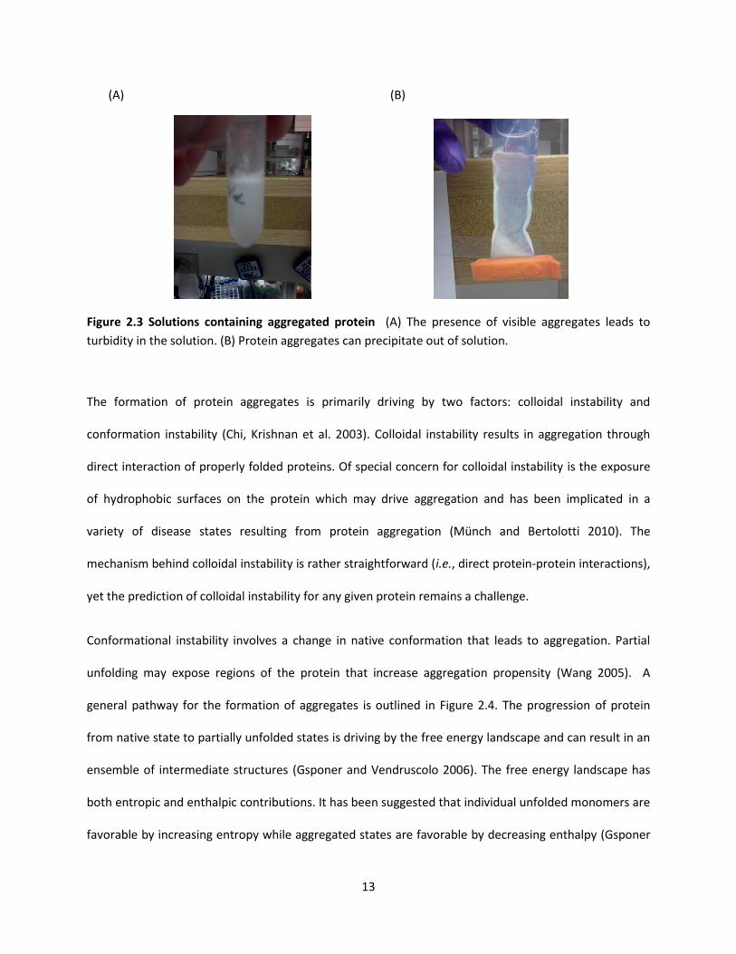
(A) (B)
Figure 2.3 Solutions containing aggregated protein (A) The presence of visible aggregates leads to
turbidity in the solution. (B) Protein aggregates can precipitate out of solution.
The formation of protein aggregates is primarily driving by two factors: colloidal instability and
conformation instability (Chi, Krishnan et al. 2003). Colloidal instability results in aggregation through
direct interaction of properly folded proteins. Of special concern for colloidal instability is the exposure
of hydrophobic surfaces on the protein which may drive aggregation and has been implicated in a
variety of disease states resulting from protein aggregation (Münch and Bertolotti 2010). The
mechanism behind colloidal instability is rather straightforward (i.e., direct protein-protein interactions),
yet the prediction of colloidal instability for any given protein remains a challenge.
Conformational instability involves a change in native conformation that leads to aggregation. Partial
unfolding may expose regions of the protein that increase aggregation propensity (Wang 2005). A
general pathway for the formation of aggregates is outlined in Figure 2.4. The progression of protein
from native state to partially unfolded states is driving by the free energy landscape and can result in an
ensemble of intermediate structures (Gsponer and Vendruscolo 2006). The free energy landscape has
both entropic and enthalpic contributions. It has been suggested that individual unfolded monomers are
favorable by increasing entropy while aggregated states are favorable by decreasing enthalpy (Gsponer

14
and Vendruscolo 2006). In many cases, aggregation may be driven through a combination of colloidal
and conformation instabilities leading to a more complicated set of pathways than that proposed in
Figure 2.4 (Wang, Nema et al. 2010).
Figure 2.4 Pathway for the formation of aggregates through conformation instability Partial unfolding
of the native protein lead to aggregation-prone intermediates. The intermediates can aggregate or
further unfolded. Figure adapted from (Wang 2005).
A variety of experimental techniques exist for the detection and assessment of protein aggregates which
can be classified as particle-based methods, separation-based methods and indirect methods
(Engelsman, Garidel et al. 2011). Particle-based methods aim to detect aggregates through identification
of particles in solution. Separation-based methods aim to separate aggregates from native protein in
solution through basis of size, following by aggregate detection. Indirect methods often utilize
spectroscopy methods to detect structural changes that are associated with protein aggregation.
Overall, experimental techniques either provide qualitative information on protein aggregation or
quantitative information such as the percentage of protein that is monomeric as opposed to aggregated.
A summary of some common experimental techniques is provided by Table 2.1. The list provided is by
means exhaustive and continual work is being performed to both improve existing aggregate detection
methods as well as develop novel techniques for aggregate detection.
Native Intermediate Unfolded
Aggregate

15
Understanding the structural properties of proteins that lead to aggregation is critical to the design of
safe and effective protein drug products, and an ability to predict aggregation propensity (i.e., the
likelihood and extent to which a protein will aggregate) with reasonable accuracy would accelerate
development. Several approaches have been developed to estimate aggregation propensity for a given
protein, which can classified into two main methods: heuristic-based methods and simulation-based
methods.

16
Tab
le 2
.1 S
um
mar
y o
f ex
per
ime
nta
l te
chn
iqu
es
com
mo
nly
uti
lize
d i
n t
he
de
tect
ion
of
pro
tein
agg
rega
tes
Tech
niq
ues
are
clas
sifi
ed
as
eith
er
par
ticl
e-b
ased
m
eth
od
s,
sep
arat
ion
-bas
ed
met
ho
ds
or
ind
irec
t m
eth
od
s.
The
qu
anti
tati
ve
ind
icat
ion
is w
ith
reg
ard
s to
th
e n
um
ber
of
aggr
egat
es p
rese
nt
in t
he
syst
em. T
able
ad
apte
d f
rom
(Li
u, A
nd
ya e
t a
l. 2
00
6;
Car
pen
ter,
Ran
do
lph
et
al.
20
10
; En
gels
man
, Gar
idel
et
al.
201
1).
17
Heuristic-based approaches attempt to use prior history on aggregation or causes of aggregation in
proteins to develop predictors for aggregation propensity. The aim of a heuristic-based approach is to
relate protein properties to experimental data on protein aggregation, with the end result being a
predictive model or algorithm that returns aggregation propensity given a measure of protein structure.
Several algorithms have been developed to predict protein aggregation in solution as a function of
structural parameters. For example, AGGRESCAN utilizes the intrinsic aggregation propensity of amino
acids obtained from an experimental aggregation database of mutated β-amyloid peptides (Conchillo-
Sole, de Groot et al. 2007). PASTA predicts the likelihood of amino acid sequences being involved in
intermolecular β-sheet formation, based on minimization of β-pairing energies (Trovato, Seno et al.
2007). Zyggregator uses factors such as protein hydrophobicity, electrostatic interactions and
alternating stretches of polar and non-polar residues to predict aggregation propensity (Tartaglia and
Vendruscolo 2008). For all of these methods, protein primary structure (amino acid sequence) is used to
return one or more scoring parameters which are indicative of the propensity of a protein to aggregate.
For instance, AGGRESCAN returns the number of aggregation prone regions, or “hot spots” in a protein.
The number of hot spots is then used to qualitatively indicate the likelihood of protein aggregation
occurring, with a larger number of hot spots corresponding to a higher likelihood. Therefore, a hallmark
of current methods is qualitative results in the form of aggregation predictors that must be interpreted.
Simulation-based methods use any of the many available molecular simulation software packages or
newly-developed tools to investigate interactions between protein molecules or dynamics within a
single protein molecule. The aim of simulation-based methods is to determine if aggregation is likely to
happen based on the energetics of protein-protein interactions (Ma and Nussinov 2006). Alternatively,
simulation-based methods can investigate the dynamics of a single protein molecule to determine if the
properties of the protein could become amenable to aggregation (Irbäck and Mohanty 2006). For
example, the spatial aggregation propensity (SAP) algorithm uses molecular simulations to determine

18
the average exposed hydrophobic surface area for a given protein, with larger exposed hydrophobic
surface areas representing increased aggregation propensity (Chennamsetty, Voynov et al. 2009). In
general, simulations are more computationally expensive than use of a model or algorithm to predict
aggregation propensity. Simulations are usually required for every system of interest. Simulation-based
methods necessitate three-dimensional structure of a protein for determination of aggregation
propensity and thus require more structural information than the heuristic-based methods described
previously. Simulation-based approaches offer advantages over current heuristic-based approaches due
to the ability for qualitative assessments (e.g., free energy calculations of protein-protein interactions)
and inclusion of formulation conditions via explicit solvent and solute modeling. Recently, hybrid
approaches have been developed to combine simulation results with heuristic model-based predictions.
The Developability Index has been constructed for monoclonal antibodies utilizing net charge and SAP
(Lauer, Agrawal et al. 2012). Additionally, the osmotic second virial coefficient (B22) has also been used
to predict protein self-association in aggregation (Chi, Krishnan et al. 2003; Printz, Kalonia et al. 2012),
though it is based on experimental measurement and not on a priori descriptors of protein structure.
2.4 APPROACHES TO AGGREGATION MINIMIZATION
Two basic approaches are taken to minimize protein aggregation in therapeutics: protein engineering
and formulation development. Protein engineering focuses on modifications to the structure of the
protein which result in reduced aggregation propensity. Formulation development attempts to minimize
aggregation through the inclusion of excipients, resulting in a multi-component product. The two
approaches differ in that protein engineering is focused on the protein molecule itself (active
compound) while formulation development is concerned with selection of excipient molecules (inactive
compounds).

19
The basis behind protein engineering is that structure of the protein determines function. Consequently,
modification of protein structure can offer improvement of certain properties while still maintaining the
intended therapeutic function. Key properties of interest for protein drugs, and therefore areas for
desired improvement, include mechanism of action, stability, bioavailability, toxicity or occurrence of
side effects, ability for production at economically viable scales and dosing/delivery requirements
(Marshall, Lazar et al. 2003). Table 2.2 provides an overview of the common targets of protein
engineering approaches. With regards to preventing aggregation, common protein engineering
strategies include replacement of cysteine residues, replacement of exposed hydrophobic residues,
charge modification and post-translation modification (Marshall, Lazar et al. 2003). Replacing free
cysteine residues can prevent aggregation that occurs due to disulfide bond formation and has been
shown to successfully reduce aggregation for commercially available protein drugs such as Proleukin
(aldesleukin, produced by Chiron) and Betaseron (interferon beta-1b, produced by Berlex/Chiron)
(Marshall, Lazar et al. 2003). Yet aggregation can still occur from the scrambling of disulfide bonds
formed from paired cysteine residues (Wang 2005). Replacement of hydrophobic residues through site-
directed mutagenesis offers an increasingly popular choice for protein engineering, including rational
protein design. For example, the SAP algorithm has been developed to identify amino acids in antibodies
with high aggregation propensity as targets for mutagenesis (Chennamsetty, Voynov et al. 2009). SAP
has also been used with total charge to provide a developability index for monoclonal antibodies (Lauer,
Agrawal et al. 2012). Protein engineering approaches may improve the stability of lyophilized protein
drugs or offer sufficient stability improvements such that lyophilization is no longer necessary.

20
Table 2.2 Common protein engineering targets for property improvementTable adapted from
(Marshall, Lazar et al. 2003).
Protein Structural Target Desired Improvement
Exposed hydrophobic residues Solubility
Binding site Interaction affinity and specificity
Loops Protease susceptibility
Core Stability and conformational control
Linear epitopes Immunogenicity
Termini Attachment of fusion partners or polyethylene glycol (PEG)
Formulation development assumes a fixed protein molecule and selects excipients to improve the drug
product properties. Figure 2.5 illustrates the general preformulation and formulation development
process. Excipients provide a variety of roles in protein drug formulation including solubilizing
compounds, stabilizers and bulking agents for lyophilized formulations (Costantino and Pikal 2004;
Strickley 2004). If possible, excipients are added to ensure stability in the aqueous solution, bypassing
the need for a lyophilized formulation. For reduction of aggregation, a common strategy is to create
favorable conditions for the native state of the protein through addition of excipients to prevent
protein-surface interactions and/or improve conformational stability. Surfactants are employed to
prevent denaturation and adherence of proteins to the surface of any variety of containers that the
protein is exposed to during manufacturing and storage, as the surfactants are more likely to bind to the
surfaces (Chang, Kendrick et al. 1996; Chi, Krishnan et al. 2003). Other excipients, such as sugars, are
added to improve conformational stability via preferential exclusion (Arakawa and Timasheff 1982).
According to preferential exclusion, sugars and other weakly interacting excipients are excluded from
the protein’s surface. The exclusion leads to an increase in free energy that is proportional to the
protein’s surface area (Arakawa and Timasheff 1982; Timasheff 1998). As a result, a compact form of the
21
protein is energetically more favorable and the native state is preferred to an unfolded or denatured
state. Excipients that bind with strong affinity to the protein surface can also affect protein stability.
Excipients that bind to the native state increase conformational stability, while excipients that have an
affinity for the unfolded state drive denaturation (Chi, Krishnan et al. 2003). Examples of molecules that
affect protein stability through binding include heme with myoglobin (increased stability) and guanidine
hydrochloride with proteins in general (decreased stability, denaturation). During formulation
development, stability concerns may justify the use of lyophilization.
Several classes of molecules are employed in lyophilized protein formulations including amino acids,
carbohydrates, polymers and surfactants (Costantino and Pikal 2004). Of special interest are
carbohydrate excipients, such as sucrose and trehalose, which have been shown repeatedly in literature
to stabilize lyophilized protein structure (Fung, Darabie et al. 2005; Li, Williams et al. 2008; Sinha, Li et
al. 2008). Many lyophilized protein formulations utilize simple sugars, disaccharides, oligosaccharides, or
sugar alcohols as stabilizers (Cleland, Langer et al. 1994). Two main theories have been proposed for
describing an excipient’s ability to stabilize biomolecules during lyophilization: water replacement and
vitrification. In the water replacement theory, stabilizing excipients are those that can substitute for
water in the dried state through hydrogen bonding with the protein (Cleland, Langer et al. 1994). The
vitrification hypothesis proposes that stabilizing excipients are those that form glasses during
lyophilization (Crowe, Carpenter et al. 1998). Vitrification is described in more detail in Section 2.4, while
water-replacement is further addressed in Section 2.5.

22
Figure 2.5 Preformulation and formulation development process diagram Adapted from (Cleland,
Langer et al. 1994).

23
2.5 VITRIFICATION – GLASS TRANSITIONS IN LYOPHILIZATION
In general, the glass transition temperature marks the change between a liquid/rubbery state and an
amorphous solid/glass state. The glass transition temperature can be measured by a variety of methods
including differential mechanical thermal analysis (DMTA) and differential scanning calorimetry (DSC)
(Rahman, Al-Marhubi et al. 2007). Due to the different features used by each method, the exact
transition temperature measured varies by method (Rahman, Al-Marhubi et al. 2007) or even by
procedure or data interpretation used for a particular method (Roos 1997). Regardless of method, the
change in features attributed to the glass transition indicate the point or region where -relaxation
processes are arrested when cooling a liquid/rubber into a glass (Gangasharan and Murthy 1995). The
transition is not a true glass-transition as defined for polymers; however, the language used to describe
the transition noted in sugars is borrowed from literature concerned with polymers. In reality, the glass
transition of sugars is related to mobility and does not describe a thermodynamic event.
For carbohydrates, -relaxation involves both structural and dielectric changes. The dielectric changes
involve the rotation of dipoles resulting in polarization while structural changes arise from local spatial
reorientations of chemical groups on the molecule (Gangasharan and Murthy 1995). The dielectric and
structural modes are coupled in carbohydrates, mainly due to the presence of hydroxyl (-OH) groups
(Gangasharan and Murthy 1995). The hydroxyl groups are polarizable and also constrain structural
rearrangements through the need to form hydrogen bonds. Every rearrangement that occurs during -
relaxation requires a hydrogen bond to be broken and then subsequently remade. The glass transition
temperature then marks the point when cooling a rubber/liquid at which there is not enough random
kinetic energy present for the necessary vibrations, reorientations and hydrogen bond shuffling resulting
in the cessation of -relaxation (Meste, Champion et al. 2002). As the molecule size increases, large
intermolecular and intramolecular cooperation is needed to make and break hydrogen bonds
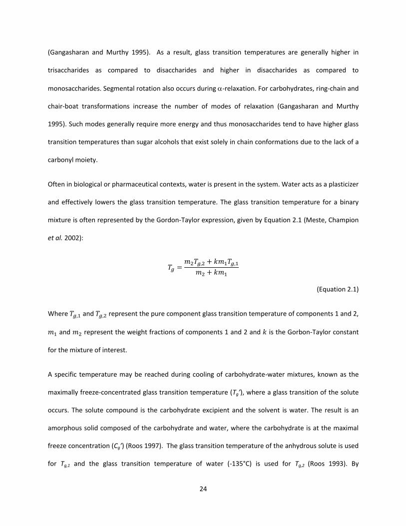
24
(Gangasharan and Murthy 1995). As a result, glass transition temperatures are generally higher in
trisaccharides as compared to disaccharides and higher in disaccharides as compared to
monosaccharides. Segmental rotation also occurs during -relaxation. For carbohydrates, ring-chain and
chair-boat transformations increase the number of modes of relaxation (Gangasharan and Murthy
1995). Such modes generally require more energy and thus monosaccharides tend to have higher glass
transition temperatures than sugar alcohols that exist solely in chain conformations due to the lack of a
carbonyl moiety.
Often in biological or pharmaceutical contexts, water is present in the system. Water acts as a plasticizer
and effectively lowers the glass transition temperature. The glass transition temperature for a binary
mixture is often represented by the Gordon-Taylor expression, given by Equation 2.1 (Meste, Champion
et al. 2002):
(Equation 2.1)
Where and represent the pure component glass transition temperature of components 1 and 2,
and represent the weight fractions of components 1 and 2 and is the Gorbon-Taylor constant
for the mixture of interest.
A specific temperature may be reached during cooling of carbohydrate-water mixtures, known as the
maximally freeze-concentrated glass transition temperature (Tg’), where a glass transition of the solute
occurs. The solute compound is the carbohydrate excipient and the solvent is water. The result is an
amorphous solid composed of the carbohydrate and water, where the carbohydrate is at the maximal
freeze concentration (Cg’) (Roos 1997). The glass transition temperature of the anhydrous solute is used
for Tg,1 and the glass transition temperature of water (-135°C) is used for Tg,2 (Roos 1993). By

25
rearrangement of Equation 2.1, the solute concentration (weight fraction) of the maximally freeze
concentrated matrix (Cg’) can be solved for, as shown in Equation 2.2.
( )
( (
))
(Equation 2.2)
If the solution is not at the proper or maximal concentration, glass formation occurs sub-Tg’ (Meste,
Champion et al. 2002). The glass transition of the anhydrous carbohydrate (Tg), the glass transition
temperature of the maximally freeze-concentrated solute (Tg’) and the maximal freeze concentration
(Cg’) are all parameters of interest when developing lyophilized protein formulations.
During lyophilization, a concentrated amorphous glass is produced during the freezing step and a mostly
water free glass is produced during the drying steps (Costantino and Pikal 2004). Initially, as a solution
with excipients is cooled, a concentrated supercooled liquid or rubbery state is formed. The melting
point of ice occurs first and represents the point where ice begins to form in the concentrated rubbery
phase (Roos 1997). Upon further cooling, the concentrated rubbery phase transitions into a
concentrated glass phase, marked by the glass transition temperature of the maximally concentrated
solute (Roos 1997). The ice is removed via sublimation as a vacuum is applied to the system (Costantino
and Pikal 2004). The amount of water remaining in the maximally freeze-concentrated glass matrix can
be estimated by Equation 2.2 (Roos 1993; Costantino and Pikal 2004). The lyophilized product
temperature is then raised and residual water in the maximally freeze-concentrated glass matrix is
removed during the drying steps. The phase transitions that occur in a lyophilized formulation are
summarized in Figure 2.6.

26
Figure 2.6 The phase transitions that occur during the lyophilization process Figure adapted from
(Roughton, Topp et al. 2012).
Roos suggested that the increase of transition temperatures could be “used in product development to
improve freeze-drying behavior and stability of dehydrated materials” (1997). A lyophilized product
must reach a temperature below both the glass transition temperature of the maximally concentrated
solute and the melting point of ice to ensure minimal water content and glass formation, restricting
protein mobility. By restricting mobility, the protein’s potential to aggregate is reduced. An appreciable
temperature difference between the glass transition temperature of the maximally concentrated solute
and the melting point of ice is also desired, as the freeze-concentrated solution is annealed between
these temperatures to ensure maximal solute concentration and minimal water content (Roos 1997).
The glass transition temperature of the anhydrous solute is important for long-term storage stability as
well, as lyophilized formulations are usually stored at temperatures at least 50°C below their glass
transition temperature (Costantino and Pikal 2004). The literature has shown glass transitions to be
dependent on chemical structure (Slade and Levine 1995), providing motivation for structure-property
model development. An ideal excipient will form a freeze-concentrate with minimal water content and
will remain a glass during drying and storage, restricting protein mobility and reducing the potential for
aggregation.
Excipient in aqueous
solution is supercooled to
form a concentrated
rubber (rubber here simply
indicates that the system is
above Tg').
Ice begins to form in the
concentrated rubbery phase, marked by the
melting point of
ice (Tm').
The excipient solution is maximally
freeze-concentrated and forms a
glass, marked by the glass transition
temperature of the maximally concentrated
solute (Tg').
Ice is removed via sublimation under a vacuum
and the temperature is
raised to remove any
residual water in the
maximally freeze-
concentrated glass matrix.
The final lyophilized product is
stored. The product
remains a glass as along as the temperature
does not exceed the glass transition
temperature of the anhydrous
solute (Tg).

27
2.6 PROTEIN-EXCIPIENT INTERACTIONS IN THE DRIED STATE
As water is the key factor in the structure that proteins adopt, dehydration or removal of water is
predicted to have a large effect on protein structure (Kuntz Jr and Kauzmann 1974). Using a poly-L-lysine
model, dehydration has been shown to result in loss of hydrogen bonds that are present in solution
(Prestrelski, Tedeschi et al. 1993). To compensate for the loss of hydrogen bonds, intermolecular
hydrogen bonds are formed and a -sheet conformation is adopted over the native random coil
conformation (Prestrelski, Tedeschi et al. 1993). A possible approach to stabilization in the dried state is
to prevent protein conformational adjustments due to the removal of water. The water replacement
hypothesis attributes protein stabilization to the replacement of protein-water interactions in aqueous
solution with protein-excipient interactions in the dried state following lyophilization.
Addition of so-called stabilizer excipients achieves partial or full preservation of protein native structure.
In particular, carbohydrate excipients have shown success when used as stabilizers. It has been
proposed that stabilization arises from a direct effect of the excipient on protein conformation
(Prestrelski, Tedeschi et al. 1993; Manning, Chou et al. 2010). Infrared spectra results have suggested
that carbohydrates hydrogen bond with proteins in the dried state and may be a requirement for the
preservation of lyophilized/dried proteins by carbohydrates (Carpenter and Crowe 1989; Prestrelski,
Tedeschi et al. 1993). The water-replacement hypothesis postulates that hydrogen bonds form between
the hydroxyl groups of carbohydrates (see Figure 2.7) and the protein backbone, mimicking the
hydrogen bonding that occurs between water and the protein backbone. Recent hydrogen-deuterium
exchange mass spectroscopy experiments support the water-replacement hypothesis, with the results
showing that certain excipients can reduce deuterium exchange in a site-specific manner (Li, Williams et
al. 2007; Li, Williams et al. 2008). Reduction of deuterium exchange indicates that the protein backbone
is protected by the inclusion of stabilizing excipients. Such protection could arise from hydrogen bonding
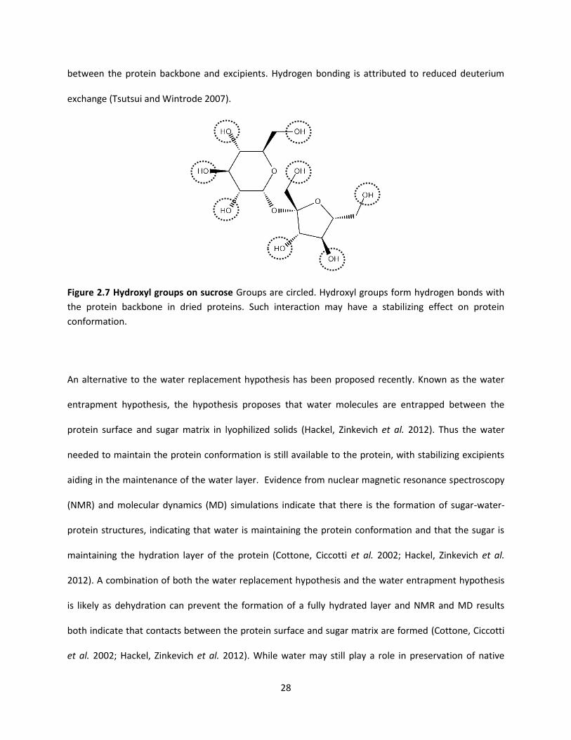
28
between the protein backbone and excipients. Hydrogen bonding is attributed to reduced deuterium
exchange (Tsutsui and Wintrode 2007).
Figure 2.7 Hydroxyl groups on sucrose Groups are circled. Hydroxyl groups form hydrogen bonds with
the protein backbone in dried proteins. Such interaction may have a stabilizing effect on protein
conformation.
An alternative to the water replacement hypothesis has been proposed recently. Known as the water
entrapment hypothesis, the hypothesis proposes that water molecules are entrapped between the
protein surface and sugar matrix in lyophilized solids (Hackel, Zinkevich et al. 2012). Thus the water
needed to maintain the protein conformation is still available to the protein, with stabilizing excipients
aiding in the maintenance of the water layer. Evidence from nuclear magnetic resonance spectroscopy
(NMR) and molecular dynamics (MD) simulations indicate that there is the formation of sugar-water-
protein structures, indicating that water is maintaining the protein conformation and that the sugar is
maintaining the hydration layer of the protein (Cottone, Ciccotti et al. 2002; Hackel, Zinkevich et al.
2012). A combination of both the water replacement hypothesis and the water entrapment hypothesis
is likely as dehydration can prevent the formation of a fully hydrated layer and NMR and MD results
both indicate that contacts between the protein surface and sugar matrix are formed (Cottone, Ciccotti
et al. 2002; Hackel, Zinkevich et al. 2012). While water may still play a role in preservation of native
29
protein structure in the dried state, stabilizers clearly play a role in maintaining protein conformation
including the formation of some direct protein-excipient interactions.
IONIC LIQUID SOLVENT DESIGN
2.7 USE OF SEPARATION MEDIA FOR AZEOTROPIC DISTILLATION AND IN SITU FERMENTATION
Solvents represent chemicals that are used to solubilize molecules of interest and may or may not be
present in the final chemical product. Of particular concern here is the use of solvents as mass
separating agents (MSA). An MSA is a chemical that aids in the separation of two or more compounds of
interest to high levels of purity. In general, an MSA is not a component of the final chemical product and
is removed and recycled following separation. Two applications for separation media are azeotropic
distillation and in situ fermentation.
Numerous binary azeotropes are encountered in chemical systems (Gmehling 1994). An azeotrope is
defined as a mixture where the liquid composition is equal to the vapor composition, resulting in a lack
of driving force for further separation to pure or mostly pure compositions. Separation of azeotropic
mixtures affects many industrial sectors due to the prevalence of such mixtures, yet separation remains
a challenging task. Azeotropes may be encountered in the solvent recovery stage following the
downstream separation of pharmaceutical and/or biochemical processes (Barton 2000; Simoni,
Chapeaux et al. 2010). Separation of azeotropic mixtures also contributes to many of the separation
tasks in the petrochemical and chemical industries (Trotta and Miracca 1997). An entrainer can
selectively interact with one of the components in an azeotrope, allowing the azeotrope to be broken
and the components separated. An basic process diagram for azeotropic distillation is presented in
Figure 2.8. A common concern with the design and operation of separation processes is the selection of
the entrainer.

30
Figure 2.8 Block flow diagram of azeotropic distillation process HC refers to the heavy component, LC
refers to the light component and E refers to the entrainer.
Industrial processes can utilize fermentation, where microorganisms convert sugars to other chemicals,
to produce chemicals of interest. A major concern in fermentation processes is separation of product
from the fermentation broth as downstream separation often requires a high energy input. Additionally,
product yield is often low in fermentation due to product inhibition. In situ product recovery during
fermentation offers a means to improve fermentation processes by reducing product inhibition and
enabling more efficient separations (Gangu, Weatherley et al. 2009). Three main in situ product
recovery processes exist: volatility-based methods, membrane-based methods and solvent-based
methods (Huang, Ramaswamy et al. 2008). Solvent-based methods provide a pathway to tunable
separations based on solvent selection. Major considerations when selecting a solvent include toxicity
towards fermentation microorganism, immiscibility with water and increased solubility of solute

31
(product) in solvent compared to water (Huang, Ramaswamy et al. 2008; Gangu, Weatherley et al.
2009). Figure 2.9 presents the basic process diagram for in situ extractive fermentation.
Figure 2.9 Block flow diagram of in situ extractive fermentation P refers to the desired product, B
refers to the fermentation broth and S refers to the solvent used for extraction.
Increasingly, the environmental impact of solvent selection must be minimized (Kerton 2009).
Additionally, material and energy inputs need to be minimized to improve process economics. Ionic
liquids represent a class of molecules that possess many desirable solvent properties and are
increasingly being considered for industrial applications. For separation processes, an optimal ionic
liquid solvent can be designed to reduce material and energy inputs and ensure feasible separation or
extraction.
2.8 IONIC LIQUIDS AS SEPARATION MEDIA
Ionic liquids (ILs) have become increasingly attractive options in solvent selection, especially for
separations. Ionic liquids are defined as salts with melting points below 100°C (Marsh, Boxall et al.
2004). Due to negligible vapor pressure, environmental concerns are reduced in comparison to many
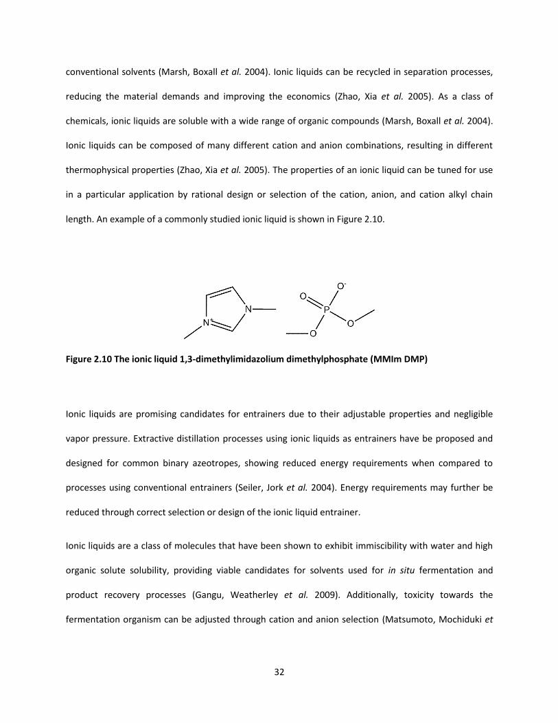
32
conventional solvents (Marsh, Boxall et al. 2004). Ionic liquids can be recycled in separation processes,
reducing the material demands and improving the economics (Zhao, Xia et al. 2005). As a class of
chemicals, ionic liquids are soluble with a wide range of organic compounds (Marsh, Boxall et al. 2004).
Ionic liquids can be composed of many different cation and anion combinations, resulting in different
thermophysical properties (Zhao, Xia et al. 2005). The properties of an ionic liquid can be tuned for use
in a particular application by rational design or selection of the cation, anion, and cation alkyl chain
length. An example of a commonly studied ionic liquid is shown in Figure 2.10.
Figure 2.10 The ionic liquid 1,3-dimethylimidazolium dimethylphosphate (MMIm DMP)
Ionic liquids are promising candidates for entrainers due to their adjustable properties and negligible
vapor pressure. Extractive distillation processes using ionic liquids as entrainers have be proposed and
designed for common binary azeotropes, showing reduced energy requirements when compared to
processes using conventional entrainers (Seiler, Jork et al. 2004). Energy requirements may further be
reduced through correct selection or design of the ionic liquid entrainer.
Ionic liquids are a class of molecules that have been shown to exhibit immiscibility with water and high
organic solute solubility, providing viable candidates for solvents used for in situ fermentation and
product recovery processes (Gangu, Weatherley et al. 2009). Additionally, toxicity towards the
fermentation organism can be adjusted through cation and anion selection (Matsumoto, Mochiduki et
33
al. 2004; Gangu, Weatherley et al. 2009). Thus the design of an ionic liquid for in situ fermentation
processes offers several, often competing, targets for required solvent properties.
FORWARD PROBLEM
2.9 DESCRIPTORS USED IN STRUCTURE-PROPERTY MODELS
The impetus for CAMD is the need for a chemical or formulation to fulfill certain characteristics. Ideally,
product characteristics can be directly linked to chemical properties. Upon identification of key
properties, property models are required for the design of molecules matching target properties.
Properties are linked to molecular structure through molecular descriptors by the generation of
structure-property models in the forward problem of CAMD.
The representation of molecule via molecular descriptors that capture relevant information is a key step
in the forward problem. Many different molecular descriptors have been considered for CAMD: group
contribution (GC) methods, graph theoretical approaches (including connectivity indices), three-
dimensional descriptors and other so-called “DRAGON” descriptors (Consonni and Todeschini 2000). In
addition to the descriptor class chosen, the functional form of the structure-property model must also
be determined. More treatment to model development is given in Section 2.10.
Group contribution models have often been used for CAMD methods as they are considered to be
simple, accurate and predictive (Harper, Gani et al. 1999). However, while GC models are commonly
applied to solvents, reliability can be a concern for classes of molecules that are inherently larger in size
(Harper, Gani et al. 1999). For example, carbohydrates can be an order of magnitude larger in molecular
weight than common organic solvents. Additionally, the types of properties that can be predicted by GC
methods has commonly been limited to thermophysical properties (Harper, Gani et al. 1999). Properties
that are dependent on three-dimensional molecular structure are not amenable to GC methods.
34
Graph theoretical methods, especially connectivity indices, have been used in quantitative structure-
property relationship (QSPR) models for a variety of systems including polymers (Camarda and Maranas
1999; Bicerano 2002) and pharmaceutical compounds (Kier, Hall et al. 1975). In graph theoretical
methods, a molecular structure is interpreted as a graph where atoms are represented by vertices and
bonds are represented by edges. Therefore, graph-based approaches capture the two-dimensional
topology of a molecular structure. Apart from bonding configuration, some graph-based descriptors
(including valence connectivity indices) capture information pertaining to the electronic configuration of
a molecule. Descriptors derived from graph theoretical approaches can be calculated with low
computational effort. In general, graph-based descriptors do not capture three-dimensional or
conformational information.
Three-dimensional based descriptors have received increase attention in the development of 3-D
quantitative structure-activity relationships (QSAR) for prediction of interaction energies for a variety of
biologically relevant systems (Cheng, Shen et al. 2002). Additionally, use of 3-D QSAR models coupled
with molecular simulation has proven fruitful in guiding computer-aided drug design efforts (Cheng,
Shen et al. 2002). A variety of 3-D descriptors can be calculated through use of computational packages
such as DRAGON (Consonni and Todeschini 2000). The advantage of 3-D descriptors is increased
information about molecular structure which can help discriminate between stereoisomers. However, 3-
D QSARs are usually limited to very defined molecular spaces and requires large computational effort for
calculation of necessary descriptors (Golbraikh, Bonchev et al. 2001). Incorporation of chirality
information in graph-based topological descriptors has been proposed as a bridge between the efficient
of graph theoretical methods and the detailed structural information provided by 3-D descriptors
(Golbraikh, Bonchev et al. 2001).
35
2.10 PROPERTY MODEL DEVELOPMENT
Development of property models requires a function form. The most basic function form is a linear
model, which can be determined through use of linear regression. Linear regression (or multiple linear
regression for multiple dependent variables) essentially utilizes optimization to provide a model with
maximum fit to the provided data. Equation 2.3 gives the general multiple linear regression model form
(Wasserman 2004).
(Equation 2.3)
Where Y is an array of independent, or response, variable values, X is a matrix of dependent variable
values and is an array of coefficient values. To maximize fit, coefficients for all dependent variables are
varied to achieve minimization of the residual sum of the squares (RSS). Equation 2.4 is used to calculate
RSS (Wasserman 2004).
∑( )
(Equation 2.4)
Where is the predicted value for observation i, is the observed value for observation i and n is the
number of observations. Determination of the coefficient values is achieved through matrix inversion of
Equation 2.3, as given by Equation 2.5 (Wasserman 2004).
( )
(Equation 2.5)

36
For functional forms utilizing non-linear model forms, the determination of coefficient values is still
determined through optimization by minimizing either RSS or another suitable indicate of fit.
While model development, especially for linear models, is relatively straightforward, the selection of
descriptors used in the model remains a subject of interest and debate. Model selection aims to choose
descriptors that maximize fit and minimize variance and prediction errors due to overfitting (Wasserman
2004). Model selection requires a score to be assigned to each model and also requires a method of
searching for models with the best score (Wasserman 2004).
Several methods exist for scoring a model. In nearly all cases, the score is based on the lack of fit provide
by the model and the number of descriptors used to generate the model. As fit will increase (albeit
usually at a decreasing rate) with the addition of more descriptors, a trade-off between underfitting and
overfitting is sought. Several common methods for scoring models include Mallow’s Cp statistic, Akaike
Information Criterion (AIC) and Bayesian Information Criterion (BIC) (Wasserman 2004). Each method
utilizes slightly different penalties for lack of fit and number of descriptors. For all cases, the model with
the minimal score is selected. Cross-validation and sensitivity analysis also provide methods of scoring
and selecting models on the basis of predictive ability and can provide further justification for the
selection of a model.
To select a model, a search must be performed for the model with the minimal score. Three methods
are used to search for models: exhaustive search, forward search and backward search (Wasserman
2004). Exhaustive search looks at all possible model combinations (number and type of descriptors).
Therefore, exhaustive search is guaranteed to return the model with the optimal score. For models with
large data sets and/or descriptor sets, exhaustive search may be too computationally expensive. In such
cases, forward search or backward search are useful. In forward search, a null model provides the
starting point. Descriptors are added one by one, selecting the descriptor that provides the lowest score
37
at each step. Once a model size is encountered that cannot provide an improvement in score compared
to the previous model size, the search is ended and the best model from the previous size is selected.
Backward search operates in a similar manner with the difference being the initial model is generated
using all available descriptors. Descriptors are then removed one by one until no further improvement
can be gained. Backward search is not possible when the number of considered descriptors exceeds the
number of observations used to develop the model.
2.11 THERMODYNAMIC PROPERTY MODELING AND PREDICTION
Thermodynamic property models seek to represent phase equilibria through mathematical means. The
determination of phase equilibria is paramount in the design of separation processes. Accordingly,
accurate and predictive models are needed for reliable separation process design. In essence, all phase
equilibria problems seek to find the solution to Equation 2.6 (Prausnitz, Lichtenthaler et al. 1999).
(Equation 2.6)
Where is the chemical potential of species i and and represent the two phases considered. For the
work presented here, fluid phases are the phases of interest. For fluid phases, Equation 2.6 can be
represented in a more useful form for species i, as provided by Equation 2.7 (Prausnitz, Lichtenthaler et
al. 1999).
(Equation 2.7)
Where is the fugacity coefficient, is vapor mole fraction, is system pressure, is activity
coefficient, is liquid mole fraction and is the fugacity at standard conditions. Of interest to the
38
work here is the determination of the activity coefficient, as provided by activity coefficient models.
Activity coefficient models provide estimation or prediction of the activity coefficient as a function of
temperature, pressure and compositon. A variety of activity coefficient models exist with the most
commonly utilized including Wilson, NRTL and UNIQUAC (Prausnitz, Lichtenthaler et al. 1999). Every
activity coefficient model is developed with certain assumptions, which can limit applicability. Of
particular interest for CAMD approaches is the UNIFAC model, a predictive group-contribution based
extension of UNIQUAC (Fredenslund, Gmehling et al. 1977). The UNIFAC model is given further
treatment in Section 4.5.
REVERSE PROBLEM
2.12 COMPUTER-AIDED MOLECULAR DESIGN (CAMD) OVERVIEW AND PROBLEM FORMULATION
The reverse problem in CAMD entails the actual design phase, where either known molecular structures
are selected from a database or novel molecular structures are proposed. In the reverse problem, target
properties values are set and molecular structures are generated which best match the target
properties. Property constraints may be employed to guide candidate selection, either during design as
rigid constraints or after design as screening criteria. The intermediary between structure and property
are the molecular descriptors used in the property models. As candidates are determined, molecular
descriptors must be calculated and used in property models to evaluate the suitability of the candidate.
Thus, a potential limiting factor in CAMD is that molecules can only be designed which are enclosed by
the chosen descriptor class.
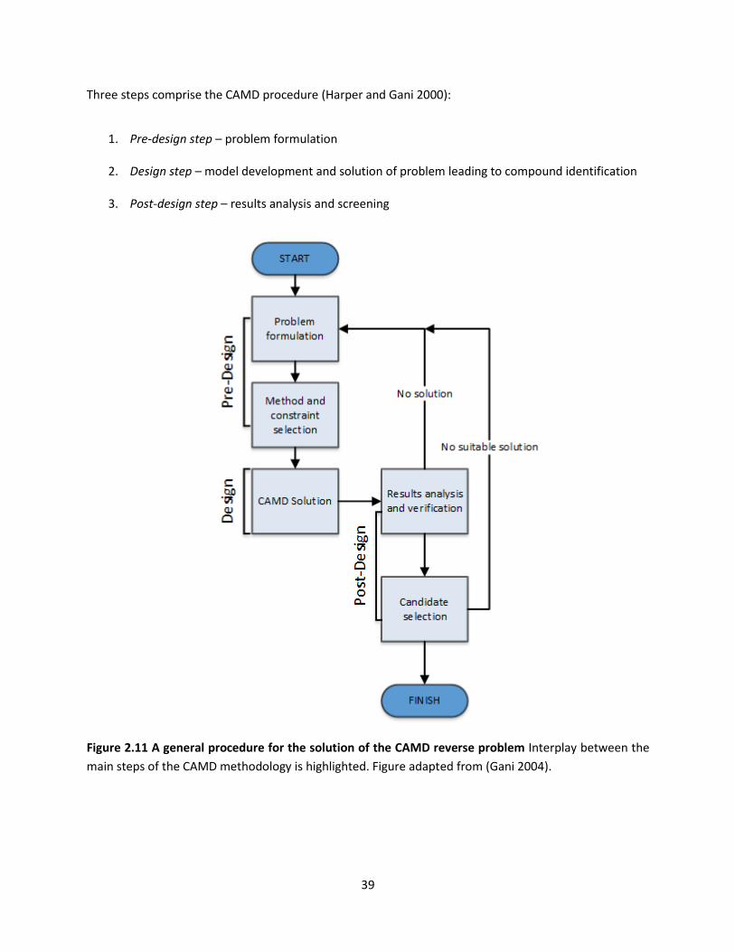
39
Three steps comprise the CAMD procedure (Harper and Gani 2000):
1. Pre-design step – problem formulation
2. Design step – model development and solution of problem leading to compound identification
3. Post-design step – results analysis and screening
Figure 2.11 A general procedure for the solution of the CAMD reverse problem Interplay between the
main steps of the CAMD methodology is highlighted. Figure adapted from (Gani 2004).
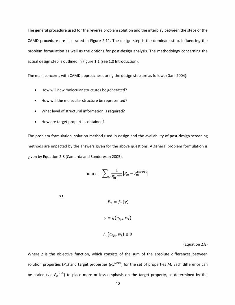
40
The general procedure used for the reverse problem solution and the interplay between the steps of the
CAMD procedure are illustrated in Figure 2.11. The design step is the dominant step, influencing the
problem formulation as well as the options for post-design analysis. The methodology concerning the
actual design step is outlined in Figure 1.1 (see 1.0 Introduction).
The main concerns with CAMD approaches during the design step are as follows (Gani 2004):
How will new molecular structures be generated?
How will the molecular structure be represented?
What level of structural information is required?
How are target properties obtained?
The problem formulation, solution method used in design and the availability of post-design screening
methods are impacted by the answers given for the above questions. A general problem formulation is
given by Equation 2.8 (Camarda and Sunderesan 2005).
∑
|
|
s.t.
( )
( )
( )
(Equation 2.8)
Where z is the objective function, which consists of the sum of the absolute differences between
solution properties (Pm) and target properties (Pmtarget) for the set of properties M. Each difference can
be scaled (via Pmscale) to place more or less emphasis on the target property, as determined by the

41
molecular properties with the highest priorities. The properties are functions of the molecular structure
(y), where the structure is provided by the chemical groups (wi) and the adjacency matrix (aijk) of the
groups. Structural constraints (hc) are employed to ensure solutions are feasible. Molecular structure
representation may vary according to implementation of CAMD. Additionally, some property models
may be used as constraints rather than targets. Property models and/or constraints often introduce
non-linearities, resulting in a mixed-integer non-linear program (MINLP).
Historically, three main approaches have been used for the solution of CAMD problems (Harper, Gani et
al. 1999; Eljack and Eden 2008):
Enumeration techniques/database search
Deterministic optimization/mathematical programming
Stochastic optimization/iterative search
Each approach has seen success in certain applications of CAMD. The approach chosen should be taken
with consideration towards the advantages and disadvantages of each approach. The three approaches
are given further attention in the following sections (2.13-2.15). A subset of CAMD involves
simultaneous product and process design and is detailed in section 2.16. Post-design methods are
examined in section 2.17.
2.13 ENUMERATION SOLUTION METHODS
The first CAMD methods employed relied on enumeration of possible solutions followed by selection of
molecules that best matched a set of target property values (Gani and Brignole 1983). Enumeration
solution methods have historically used group contribution property models. The approach of
enumeration methods is to determine the number and types of functional groups that best satisfy a set

42
of target properties. Given the functional groups determined, molecular structures are identified that
are comprised of all the functional groups selected.
A general procedure for CAMD by enumeration follows (Gani, Nielsen et al. 1991):
1. Preselect the types of groups that will be used to provide solutions. Additionally, the properties
of interest with set target values must be identified. Rules for the formation of feasible
compounds from the groups selected must be established.
2. All chemically feasible molecules are generated.
3. Solution reduction is performed by property screening. Properties are predicted for the set of
chemically feasible molecules. Molecules that match the target properties are retained while all
other solutions are discarded.
4. Post-design methods such as process simulation are utilized to rank remaining solutions on basis
of performance index. Screening of secondary properties may also be used to reduce the
amount of solutions considered.
Vital to the use of enumeration solution methods is the ability to generate all feasible chemical
structures. For design cases with large numbers of possible solutions, the generation of all possible
solutions may prove computationally restrictive. However, for small cases the enumeration approach
can identify optimal solution. Incorporation of multi-level molecular representation (e.g., higher order
group contribution methods) provides opportunities for more rigorous property prediction (Harper and
Gani 2000).
2.14 DETERMINISTIC SOLUTION METHODS
Deterministic methods seek to find a global optimum to a mixed-integer linear program (MILP) or
mixed-integer non-linear program (MINLP) through derivative-based solutions. Use of deterministic
43
methods requires mathematical constraints to effectively limit the search space. Solution of a MILP is
almost always performed by branch and bound methods (Edgar, Himmelblau et al. 2001). Often a MINLP
results from problem formulation. When a MINLP results, the determination of a global optimum is not
guaranteed. By far, the most commonly used method to solve MINLPs in CAMD utilizes the optimization
solver DICOPT (http://www.gams.com/dd/docs/solvers/dicopt.pdf), which is available in the
optimization software GAMS (http://www.gams.com/).
DICOPT solves MINLPs through the use of outer approximation, which is an iterative process that solves
two sub-problems each iteration (Duran and Grossmann 1986; Floudas 1995). The first sub-problem is
the solution of a non-linear program (NLP), which is formed by fixing the integer values of the original
MINLP problem. Optimization is then performed over the continuous variables, with the provided
solution being a lower bound to the original MINLP problem (Edgar, Himmelblau et al. 2001). The next
sub-problem is the solution of a MILP. The continuous variable portion of the objective function is
replaced with a constant. The constant is constrained to maintain equivalence to the original MINLP
formulation. Solution of the MILP sub-problem optimizes over both the integer and continuous
variables, with the provided solution being an upper bound to the original MINLP problem (Edgar,
Himmelblau et al. 2001). If the problem is convex, the upper and lower bounds will converge to the
optimal solution for the original MINLP problem in a finite number of iterations (Duran and Grossmann
1986; Floudas 1995). In addition to outer approximation, other approaches have also been considered
for solution of MINLPs in CAMD problems, but are not given further treatment here (Sahinidis and
Tawarmalani 2000; Karunanithi, Achenie et al. 2006).
2.15 STOCHASTIC SOLUTION METHODS
Stochastic methods employ iterative processes to determine locally optimal solutions. Depending on the
method, different rules or moves are used to proceed from one solution to another. Stochastic methods
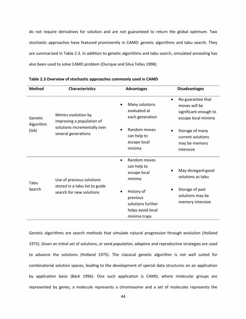
44
do not require derivatives for solution and are not guaranteed to return the global optimum. Two
stochastic approaches have featured prominently in CAMD: genetic algorithms and tabu search. They
are summarized in Table 2.3. In addition to genetic algorithms and tabu search, simulated annealing has
also been used to solve CAMD problem (Ourique and Silva Telles 1998).
Table 2.3 Overview of stochastic approaches commonly used in CAMD
Method Characteristics Advantages Disadvantages
Genetic
Algorithm
(GA)
Mimics evolution by
improving a population of
solutions incrementally over
several generations
Many solutions
evaluated at
each generation
Random moves
can help to
escape local
minima
No guarantee that
moves will be
significant enough to
escape local minima
Storage of many
current solutions
may be memory
intensive
Tabu
Search
Use of previous solutions
stored in a tabu list to guide
search for new solutions
Random moves
can help to
escape local
minima
History of
previous
solutions further
helps avoid local
minima traps
May disregard good
solutions as tabu
Storage of past
solutions may be
memory intensive
Genetic algorithms are search methods that simulate natural progression through evolution (Holland
1975). Given an initial set of solutions, or seed population, adaptive and reproductive strategies are used
to advance the solutions (Holland 1975). The classical genetic algorithm is not well suited for
combinatorial solution spaces, leading to the development of special data structures on an application
by application basis (B c 199 ). One such application is CAMD, where molecular groups are
represented by genes, a molecule represents a chromosome and a set of molecules represents the

45
population (Venkatasubramanian, Chan et al. 1994). Moves mimicking adaptation and reproduction are
used to alter the population in each iteration or generation. Moves mimicking adaption can be thought
of as local moves, while reproductive-inspired moves are global moves. The suitability of solutions is
determined by their fitness, which in turn determines the likelihood of a solution to become a parent
(Venkatasubramanian, Chan et al. 1994). Parents are used to generate the population for the next
generation. The search continues until a predetermined number of generations is reached. The search is
then terminated, returning the solution with the highest fitness.
Tabu search is a heuristic approach which guides a local search through use of previous solution history
(Glover 1989; Lin, Chavali et al. 2005). Tabu search relies on recently visited solutions, which are stored
in a tabu list. Local moves are made to change a previous solution to a new solution. If a new solution is
too similar to a solution stored in the tabu list, it is deemed tabu and discarded (Glover 1989; Lin,
Chavali et al. 2005). Similarity is determined by the tabu criterion. In this manner, the search for
solutions is a constrained search (Glover 1989). The search space is more effectively scanned and local
minima can be escaped to search for better solutions. If a tabu solution is the best solution yet
encountered, the tabu criterion can be overridden via aspiration (Glover 1989). After a predetermined
number of non-improving iterations, the search is terminated and the best solution is returned (Glover
1989).
2.16 INTEGRATED PRODUCT-PROCESS DESIGN
Product and process design employ similar solution methods and are both utilized to improve chemical
production processes. Consequently the simultaneous design of both product and process has been
pursued for various applications, especially for separation design (Eden, Jørgensen et al. 2004;
Roughton, Christian et al. 2012). For separation design, the designed product is often a solvent for use in
achieving the desired separation. The desired process performance is used to determine molecule

46
property targets and constraints. The properties are in turn used to determine optimal chemical
structures. In effect, integrated process design involves solving two reverse problems (see Figure 2.12).
The final solution contains the design variables for the process as well as the molecules that satisfy the
necessary property targets. By coupling molecular design with process design, process performance can
be expected to improve as optimal solvents are identified and used in the necessary separations.
Figure 2.12 Overview of integrated product and process design Each design process generates
parameters that are used to constrain the other design problem. Adapted from (Eden, Jørgensen et al.
2004).
2.17 POST-DESIGN METHODS
Post-design methods are used in CAMD to further screen the candidates generated in the design phase.
The simplest post-design method is the use of secondary properties to screen the candidates. Such
properties may require higher-dimensional structural information than is utilized during the design
phase due to computational limitations (Harper and Gani 2000). A more detailed analysis of candidates
is provided by the use of molecular modeling. A three-dimensional model is generated for a given
candidate through the use of energy minimization. The end result is a 3-D molecular structure that can
be used to obtain values for properties that require 3-D structural information (Harper, Gani et al. 1999).

47
An common example is toxicity towards various organisms, which is often predicted via a 3-D QSAR
(Akamatsu 2002). Experimental verification is needed for final candidate selection and is beginning to be
implemented in CAMD frameworks (Conte, Gani et al. 2011; Conte, Gani et al. 2012).
48
3.0 EXPERIMENTAL METHODS
The following chapter describes in detail the experimental plan used in the work as well as all relevant
experimental methods that were used to generate data for the forward problem. Methods that were
performed by the author include the experimental procedure used for generation of the data. The
theory behind hydrogen-deuterium exchange mass spectroscopy is detailed as experimental data
obtained from the method is used in conjunction with simulations to investigate protein-excipient
interactions (See Section 7.0). Refer to the references cited for detailed information concerning the
experimental setup and procedure.
3.1 EXPERIMENTAL OVERVIEW
The experiments done by the author were performed to evaluate the effect of excipient selection on
aggregation following lyophilization. The following methods were performed by the author and all data
pertaining to the methods were generated by the author for the data set used to generate models
describing post-lyophilization protein loss as a function of excipient structure: ultraviolet-visible light
spectrophotometry, size-exclusion chromatography, sodium-dodecyl-sulfate polyacrylamide gel
electrophoresis and powder x-ray diffraction. Figure 3.1 displays the overall experimental approach.

49
Figure 3.1 Overview of experimental procedure used by author The aim of the experiments was to
characterize aggregation following lyophilization for several different excipient and protein choices.
Additional experimental results were obtained from literature for use in modeling building for the
forward problem. The corresponding references contain information concerning the experimental setup
and procedure. Material procurement, sample preparation and lyophilization for the experiments done
by the author follow.
3.1.1 Materials
The following proteins were considered in the study: -amylase, bovine serum albumin (BSA),
ovalbumin, ribonuclease A (RNAse A) and soybean trypsin inhibitor. All proteins were acquired from
Sigma-Aldrich (St. Louis, MO) except trypsin inhibitor, which was obtained from Worthington
Biochemical Corporation (Lakewood, NJ). Table 3.1 lists key biophysical properties for each protein.
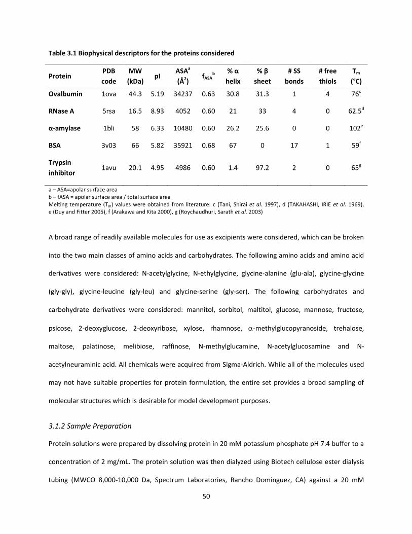
50
Table 3.1 Biophysical descriptors for the proteins considered
Protein PDB
code
MW
(kDa) pI
ASAa
(Å2) fASA
b % α
helix
% β
sheet
# SS
bonds
# free
thiols
Tm
(°C)
Ovalbumin 1ova 44.3 5.19 34237 0.63 30.8 31.3 1 4 76c
RNase A 5rsa 16.5 8.93 4052 0.60 21 33 4 0 62.5d
α-amylase 1bli 58 6.33 10480 0.60 26.2 25.6 0 0 102e
BSA 3v03 66 5.82 35921 0.68 67 0 17 1 59f
Trypsin
inhibitor 1avu 20.1 4.95 4986 0.60 1.4 97.2 2 0 65g
a – ASA=apolar surface area b – fASA = apolar surface area / total surface area Melting temperature (Tm) values were obtained from literature: c (Tani, Shirai et al. 1997), d (TAKAHASHI, IRIE et al. 1969), e (Duy and Fitter 2005), f (Arakawa and Kita 2000), g (Roychaudhuri, Sarath et al. 2003)
A broad range of readily available molecules for use as excipients were considered, which can be broken
into the two main classes of amino acids and carbohydrates. The following amino acids and amino acid
derivatives were considered: N-acetylglycine, N-ethylglycine, glycine-alanine (glu-ala), glycine-glycine
(gly-gly), glycine-leucine (gly-leu) and glycine-serine (gly-ser). The following carbohydrates and
carbohydrate derivatives were considered: mannitol, sorbitol, maltitol, glucose, mannose, fructose,
psicose, 2-deoxyglucose, 2-deoxyribose, xylose, rhamnose, -methylglucopyranoside, trehalose,
maltose, palatinose, melibiose, raffinose, N-methylglucamine, N-acetylglucosamine and N-
acetylneuraminic acid. All chemicals were acquired from Sigma-Aldrich. While all of the molecules used
may not have suitable properties for protein formulation, the entire set provides a broad sampling of
molecular structures which is desirable for model development purposes.
3.1.2 Sample Preparation
Protein solutions were prepared by dissolving protein in 20 mM potassium phosphate pH 7.4 buffer to a
concentration of 2 mg/mL. The protein solution was then dialyzed using Biotech cellulose ester dialysis
tubing (MWCO 8,000-10,000 Da, Spectrum Laboratories, Rancho Dominguez, CA) against a 20 mM
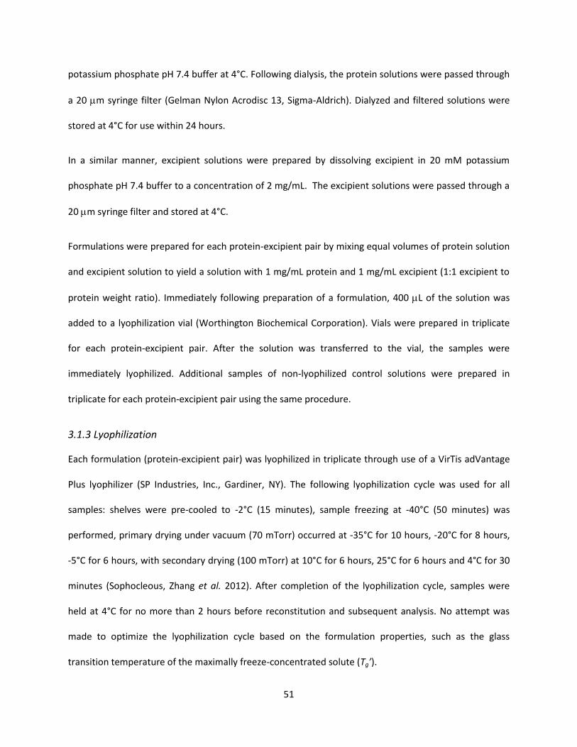
51
potassium phosphate pH 7.4 buffer at 4°C. Following dialysis, the protein solutions were passed through
a 20 m syringe filter (Gelman Nylon Acrodisc 13, Sigma-Aldrich). Dialyzed and filtered solutions were
stored at 4°C for use within 24 hours.
In a similar manner, excipient solutions were prepared by dissolving excipient in 20 mM potassium
phosphate pH 7.4 buffer to a concentration of 2 mg/mL. The excipient solutions were passed through a
20 m syringe filter and stored at 4°C.
Formulations were prepared for each protein-excipient pair by mixing equal volumes of protein solution
and excipient solution to yield a solution with 1 mg/mL protein and 1 mg/mL excipient (1:1 excipient to
protein weight ratio). Immediately following preparation of a formulation, 400 L of the solution was
added to a lyophilization vial (Worthington Biochemical Corporation). Vials were prepared in triplicate
for each protein-excipient pair. After the solution was transferred to the vial, the samples were
immediately lyophilized. Additional samples of non-lyophilized control solutions were prepared in
triplicate for each protein-excipient pair using the same procedure.
3.1.3 Lyophilization
Each formulation (protein-excipient pair) was lyophilized in triplicate through use of a VirTis adVantage
Plus lyophilizer (SP Industries, Inc., Gardiner, NY). The following lyophilization cycle was used for all
samples: shelves were pre-cooled to -2°C (15 minutes), sample freezing at -40°C (50 minutes) was
performed, primary drying under vacuum (70 mTorr) occurred at -35°C for 10 hours, -20°C for 8 hours,
-5°C for 6 hours, with secondary drying (100 mTorr) at 10°C for 6 hours, 25°C for 6 hours and 4°C for 30
minutes (Sophocleous, Zhang et al. 2012). After completion of the lyophilization cycle, samples were
held at 4°C for no more than 2 hours before reconstitution and subsequent analysis. No attempt was
made to optimize the lyophilization cycle based on the formulation properties, such as the glass
transition temperature of the maximally freeze-concentrated solute (Tg’).

52
3.2 ULTRAVIOLET-VISIBLE LIGHT SPECTROPHOTOMETRY (UV-VIS)
3.2.1 Theory
UV-Vis is a technique that measures absorbance of light by a molecule at any given wavelength. The
absorption of light is accompanied by a transition in the molecule from lower energy state to a higher
energy state, via energy provided by the photon of light (Van Holde, Johnson et al. 2006). The transitions
typically associated with ultraviolet and visible light absorption are electronic transitions of the valence
shell electrons, where electrons are excited from an occupied or ground state orbital to an unoccupied
or excited state orbital (Van Holde, Johnson et al. 2006). Absorption occurs if the energy of the photon
at a particular wavelength is equal to the difference in energy between the ground state and the excited
state. The energy absorbed from the photon is usually lost as heat. By comparing the emission of light
through a sample and a control, differences observed are used to construct the absorption spectra of
the sample. Chromophores are chemical groups that absorb light at particular wavelengths and thus
have characteristic absorption spectra (Van Holde, Johnson et al. 2006).
Proteins contain several chromophores: peptide bond, aromatic residues (phenylalanine, tryptophan
and tyrosine), prosthetic groups and metal cations (see Figure 3.2). Absorbance due to the peptide bond
is the strongest observed and occurs around a wavelength of 185-195 nm, depending on the protein’s
secondary structure (Martin, Sinko et al. 2011). Absorbance from the range of 250-300 nm corresponds
to absorbance by the aromatic residues in the protein. Prosthetic groups and metal cations may have
absorbance at varying wavelengths according to the species of interest. Absorbance past 300 nm is
associated with light scattering (Martin, Sinko et al. 2011). A typical UV-vis spectrum for a protein is
shown in Figure 3.3.
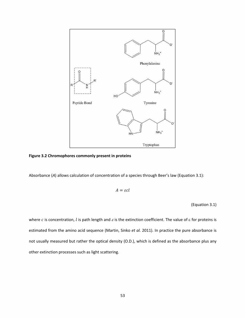
53
Figure 3.2 Chromophores commonly present in proteins
Absorbance (A) allows calculation of concentration of a species through Beer’s law (Equation 3.1):
(Equation 3.1)
where is concentration, is path length and is the extinction coefficient. The value of for proteins is
estimated from the amino acid sequence (Martin, Sinko et al. 2011). In practice the pure absorbance is
not usually measured but rather the optical density (O.D.), which is defined as the absorbance plus any
other extinction processes such as light scattering.
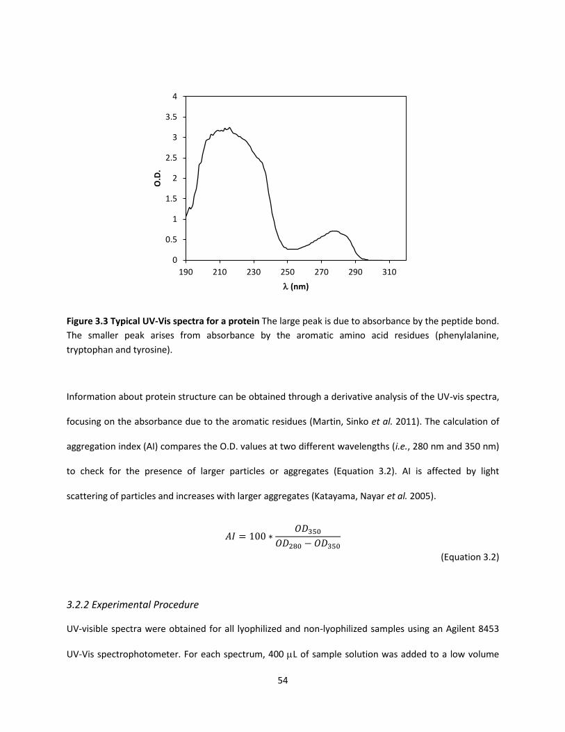
54
Figure 3.3 Typical UV-Vis spectra for a protein The large peak is due to absorbance by the peptide bond.
The smaller peak arises from absorbance by the aromatic amino acid residues (phenylalanine,
tryptophan and tyrosine).
Information about protein structure can be obtained through a derivative analysis of the UV-vis spectra,
focusing on the absorbance due to the aromatic residues (Martin, Sinko et al. 2011). The calculation of
aggregation index (AI) compares the O.D. values at two different wavelengths (i.e., 280 nm and 350 nm)
to check for the presence of larger particles or aggregates (Equation 3.2). AI is affected by light
scattering of particles and increases with larger aggregates (Katayama, Nayar et al. 2005).
(Equation 3.2)
3.2.2 Experimental Procedure
UV-visible spectra were obtained for all lyophilized and non-lyophilized samples using an Agilent 8453
UV-Vis spectrophotometer. For each spectrum, 400 L of sample solution was added to a low volume
0
0.5
1
1.5
2
2.5
3
3.5
4
190 210 230 250 270 290 310
O.D
.
l (nm)

55
cuvette. Wavelengths were collected from 200-600 nm using an integration time of 10 seconds and an
interval of 1 nm. The aggregation index (AI) was calculated for each sample given the optical density
values at 280 and 350 nm (see Equation 3.2).
3.3 SIZE-EXCLUSION CHROMATOGRAPHY (SEC)
3.3.1 Theory
SEC is used to separate molecules on the basis of size and shape (see Figure 3.4). A sample containing
molecular species of varying sizes is injected upstream of the column. The sample flows through the
system through use of a mobile phase, which is pumped at a constant rate. The mobile phase often
contains a buffer to maintain the pH of the sample. The column used in SEC is packed with a porous
matrix which provides the separation ability. Gel beads comprise the matrix or fixed phase of the
column, resulting in a cross-linked network of pores (Rosenberg 2005). Separation of molecules is based
on the size of the pores in the beads, with larger molecules being unable to enter the pores and thus
eluting at a faster time. Both molecular weight (size) and the three-dimensional conformation (shape) of
the molecule contribute to a protein’s ability to enter a pore. Adsorption of protein to the column
matrix is a concern in SEC, preventing protein from eluting in a timely manner if at all. For analysis of
protein samples, high salt concentrations are used in the mobile phase to curtail protein adsorption to
the column matrix (Arakawa, Ejima et al. 2010).
SEC is often coupled with UV-vis spectrophotometry through inclusion of an inline UV detector following
the SEC column. Determination of UV absorption immediately following elution form the column allows
for quantitative measurement of the amount of molecules eluting at a given time. UV absorption values
are either taken at a few specific wavelengths (e.g., 280 nm for proteins) or an entire absorption
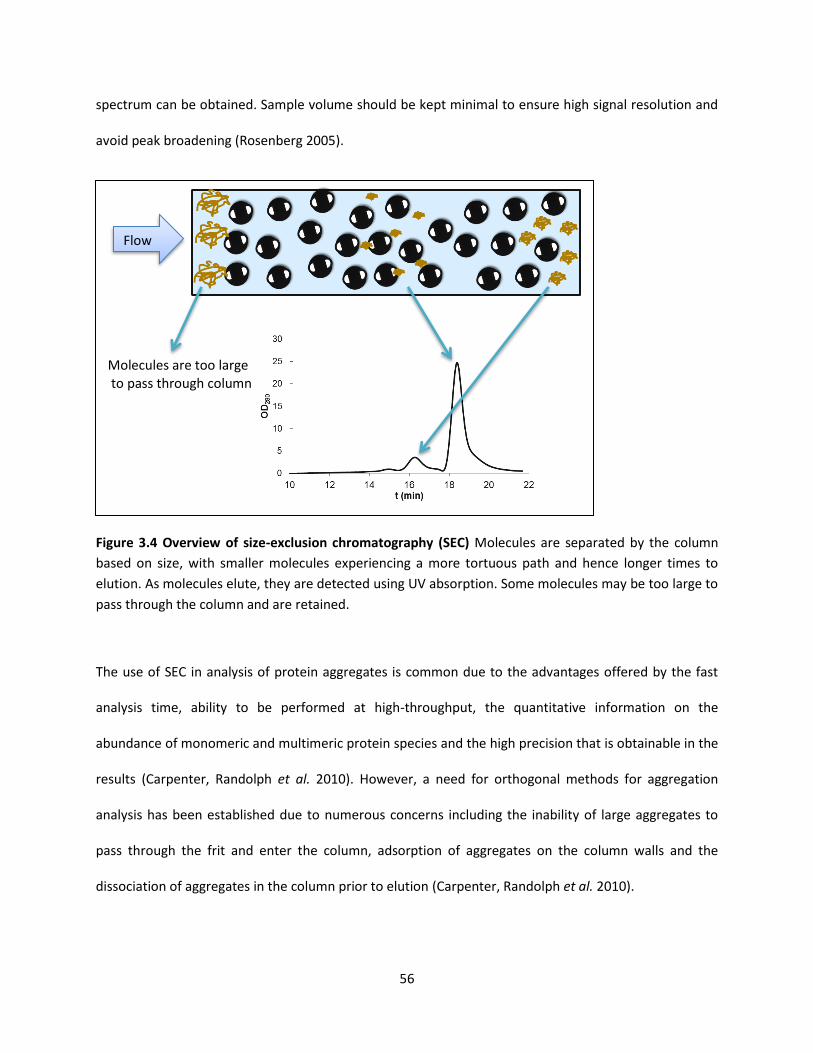
56
spectrum can be obtained. Sample volume should be kept minimal to ensure high signal resolution and
avoid peak broadening (Rosenberg 2005).
Figure 3.4 Overview of size-exclusion chromatography (SEC) Molecules are separated by the column
based on size, with smaller molecules experiencing a more tortuous path and hence longer times to
elution. As molecules elute, they are detected using UV absorption. Some molecules may be too large to
pass through the column and are retained.
The use of SEC in analysis of protein aggregates is common due to the advantages offered by the fast
analysis time, ability to be performed at high-throughput, the quantitative information on the
abundance of monomeric and multimeric protein species and the high precision that is obtainable in the
results (Carpenter, Randolph et al. 2010). However, a need for orthogonal methods for aggregation
analysis has been established due to numerous concerns including the inability of large aggregates to
pass through the frit and enter the column, adsorption of aggregates on the column walls and the
dissociation of aggregates in the column prior to elution (Carpenter, Randolph et al. 2010).
Flow
Molecules are too large to pass through column
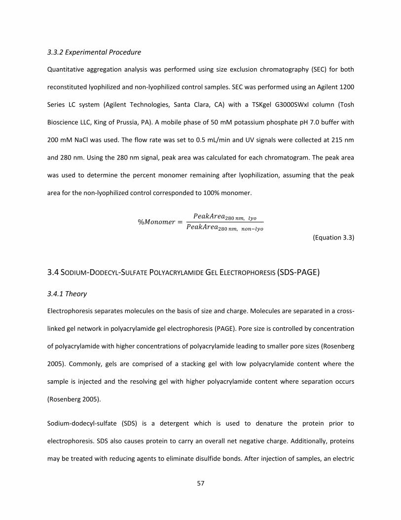
57
3.3.2 Experimental Procedure
Quantitative aggregation analysis was performed using size exclusion chromatography (SEC) for both
reconstituted lyophilized and non-lyophilized control samples. SEC was performed using an Agilent 1200
Series LC system (Agilent Technologies, Santa Clara, CA) with a TSKgel G3000SWxI column (Tosh
Bioscience LLC, King of Prussia, PA). A mobile phase of 50 mM potassium phosphate pH 7.0 buffer with
200 mM NaCl was used. The flow rate was set to 0.5 mL/min and UV signals were collected at 215 nm
and 280 nm. Using the 280 nm signal, peak area was calculated for each chromatogram. The peak area
was used to determine the percent monomer remaining after lyophilization, assuming that the peak
area for the non-lyophilized control corresponded to 100% monomer.
(Equation 3.3)
3.4 SODIUM-DODECYL-SULFATE POLYACRYLAMIDE GEL ELECTROPHORESIS (SDS-PAGE)
3.4.1 Theory
Electrophoresis separates molecules on the basis of size and charge. Molecules are separated in a cross-
linked gel network in polyacrylamide gel electrophoresis (PAGE). Pore size is controlled by concentration
of polyacrylamide with higher concentrations of polyacrylamide leading to smaller pore sizes (Rosenberg
2005). Commonly, gels are comprised of a stacking gel with low polyacrylamide content where the
sample is injected and the resolving gel with higher polyacrylamide content where separation occurs
(Rosenberg 2005).
Sodium-dodecyl-sulfate (SDS) is a detergent which is used to denature the protein prior to
electrophoresis. SDS also causes protein to carry an overall net negative charge. Additionally, proteins
may be treated with reducing agents to eliminate disulfide bonds. After injection of samples, an electric
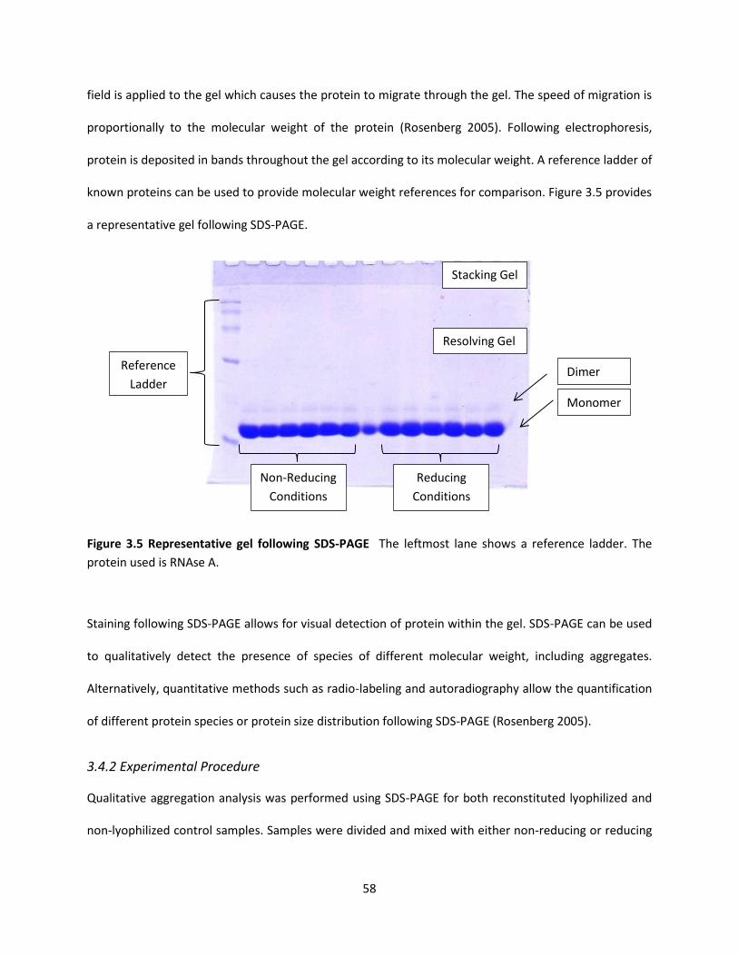
58
field is applied to the gel which causes the protein to migrate through the gel. The speed of migration is
proportionally to the molecular weight of the protein (Rosenberg 2005). Following electrophoresis,
protein is deposited in bands throughout the gel according to its molecular weight. A reference ladder of
known proteins can be used to provide molecular weight references for comparison. Figure 3.5 provides
a representative gel following SDS-PAGE.
Figure 3.5 Representative gel following SDS-PAGE The leftmost lane shows a reference ladder. The
protein used is RNAse A.
Staining following SDS-PAGE allows for visual detection of protein within the gel. SDS-PAGE can be used
to qualitatively detect the presence of species of different molecular weight, including aggregates.
Alternatively, quantitative methods such as radio-labeling and autoradiography allow the quantification
of different protein species or protein size distribution following SDS-PAGE (Rosenberg 2005).
3.4.2 Experimental Procedure
Qualitative aggregation analysis was performed using SDS-PAGE for both reconstituted lyophilized and
non-lyophilized control samples. Samples were divided and mixed with either non-reducing or reducing
Reference
Ladder
Stacking Gel
Resolving Gel
Non-Reducing
Conditions
Reducing
Conditions
Dimer
Monomer

59
(containing -mercaptoethanol) loading buffer containing bromophenol blue for staining. Samples were
vortexed for 10 min and then heated for 5 min at 95°C. Samples were allowed to cool and were then
loaded into 10% or 12% polyacrylamide gels. Precision Plus Protein Dual Xtra Standards (Bio-Rad,
Hercules, CA) were used as a reference ladder. SDS-PAGE was performed using a Mini-PROTEAN Tetra
cell electrophoresis instrument attached to a PowerPac Basic power supply (Bio-Rad). After completion
of electrophoresis, the gels were removed and stained with Coomassie Brilliant Blue R-250 staining
solution for 30 min and then destained for approximately 24 hrs on a rocking platform (VWR
International, Radnor, PA).
3.5 POWDER X-RAY DIFFRACTION (PXRD)
3.5.1 Theory
Powder x-ray diffraction emits x-rays at a powdered solid sample and measures the resulting
diffraction pattern. X-rays are sent from a source (e.g., x-ray tube) and collide with the sample at a
specified incident angle (). As the x-rays collide with atoms in the solid, the x-rays are scattered.
An x-ray detector is used to detect any x-rays that are deflected at an angle of twice the incident
angle (in reference to the x-ray beam sent from the source), referred to as 2. The detection of x-
rays is represented as the intensity. The incident angle is changed repeatedly to allow detection of
diffraction patterns across a range of 2 values. A typical PXRD setup is shown in Figure 3.6.

60
Figure 3.6 Diagram of typical powder x-ray diffraction setup X-rays are sent from the source (x-ray
tube) and are reflected back to the detector at an angle referred to as the incident angle (). 2 is equal
to two times . Figure adapted from (Speakman).
Arrangement of the atoms in a sample produces a characteristic diffraction pattern. Bragg’s law
describes the conditions that must be satisfied for diffraction to occur at a given incident angle ():
(Equation 3.4)
Where l is the wavelength of the x-ray and is fixed and dhkl is a characteristic vector defined by the
crystal geometry. A crystal has repeating units of atomic structure, referred to as unit cells
(Shackelford 2009). The unit cell represents the maximal symmetric unit in the material and has a
characteristic shape and size that determines dhkl (Speakman ; Shackelford 2009). The unit cell in a
crystal has atomic planes which are attributed to the diffraction peaks observed in a sample. As
the unit cell is repeated, diffraction at the angle incident to the plane occurs frequently resulting in
a sharp peak with high intensity in the observed diffraction pattern.
2
X-ray tube
Sample
Detector

61
While pxrd has several applications, the focus here is the use of pxrd to determine whether a sample is
crystalline or amorphous. On a qualitative basis, a sample can be classified as either largely amorphous
or largely crystalline based on the overall diffraction pattern observed. Amorphous solids have no long
range order and thus show no diffraction pattern, instead displaying what is referred to as an
“amorphous halo” (see Figure 3.7). Crystalline solids are highly ordered and only show diffraction at
certain wavelengths based on the crystal structure. The resulting diffraction pattern is characterized by a
few sharp peaks of high intensity (see Figure 3.7). The discernible visual differences in the diffraction
patterns often allows for a general qualitative classification of either largely amorphous or largely
crystalline. Quantitatively, pxrd can be used to calculate the percent crystallinity of a sample by dividing
the intensity of a peak observed in a given sample by the intensity of the peak in a pure crystalline
control (Clas, Faizer et al. 1995). For multiple peaks, the intensities are summed for both the sample and
the pure crystalline control and then the ratio is determined. Low percent crystallinity corresponds to a
sample that is largely amorphous. For small molecule drug development, the exact percent crystallinity
is often of interest as it relates to bioavailability (Clas, Faizer et al. 1995). However for the experiments
conducted here, the main concern was whether any given formulation was largely amorphous following
lyophilization for which a qualitative approach was sufficient.

62
Figure 3.7 Representative x-ray diffraction patterns (A) amorphous material and (B) crystalline material
showing intensity (<I>) versus 2. Figure adapted from (Speakman).
3.5.2 Experimental Procedure
Samples for PXRD analysis were prepared similarly to the method stated previously except protein and
excipient solutions were made to concentrations of 10 mg/mL, yielding formulation concentrations of 5
mg/mL protein and 5 mg/mL excipient (1:1 excipient to protein weight ratio). The same sample volume
of 400 L was transferred to the lyophilization vials for each protein-excipient pair. Samples were
lyophilized using the previously mentioned lyophilization cycle. Following lyophilization, confirmation
that the samples were amorphous was performed by collecting X-ray diffractograms using a Scintag X2
- diffractometer (Scintag Inc., Cupertino, CA) equipped with a Cu K anode operating at a wavelength
of 1.5406 Å.
Due to the large amount of formulations considered, a smaller subset was selected for PXRD analysis.
JMP statistical software (SAS, www.jmp.com ) was used to randomly select a minimal number of
<I>
2
A
B

63
formulations for analysis such that each protein was selected at least once, each excipient was selected
at least once and each sugar alcohol excipient was selected at least twice. 20 formulations were
selected and from the set of 20, 6 were randomly selected to be done in replicate. Only carbohydrate
excipients were considered.
3.6 HYDROGEN-DEUTERIUM EXCHANGE MASS SPECTROSCOPY (HX-MS)
3.6.1 Theory
Hydrogens bonded to the amide nitrogen (See Figure 3.8) in the protein backbone can exchange with
deuteriums when exposed to deuterated water (D2O). The reaction can be catalyzed either acid (D3O+)
or base (OD-). The exchange rate of the amide hydrogens can occur over a wide range of time, with
some exchanging in milliseconds and others in days.
Figure 3.8 A peptide bond, which forms between amino acids to construct the protein backbone The
hydrogen bonded to the amide nitrogen is highlighted in red. The hydrogen participates in exchange
with deuterium during HX experiments.
The exchange rate is highly dependent on the degree of solvent protection and hydrogen bonding.
Buried residues or residues with an amide hydrogen that participating in hydrogen bonding are resistant
to exchange, where surface residue freely exchange hydrogen for deuterium (Tsutsui and Wintrode
2007). Hydrogen exchange is also impacted by the flexibility of the protein’s conformation, both locally
and overall. Fluctuations in the protein’s structure allow solvent penetration and subsequent exchange.
The exchange rate is given by Equation 3.5 (Tsutsui and Wintrode 2007):
64
(Equation 3.5)
Where is the rate of conformational changes that result in unfolding, is the rate of
conformational changes that result in folding, is the chemical rate of exchange between a hydrogen
and a deuterium and is the observed rate of exchange. The overall observed exchange can be
divided into two regimes: the EX1 regime ( >> ) and the EX2 regime ( >> ). In EX1, the
protein exhibits multiple conformations and slowly interconverts between conformations, allow
exchange to occur (Tsutsui and Wintrode 2007). The observed exchange rate depends only on the rate
of unfolding. The EX1 regime is often induced through use of denaturants. More frequently the EX2
regime is observed, where local conformational changes exposing amide hydrogens may occur multiple
times before exchange can occur (Tsutsui and Wintrode 2007). The observed rate is therefore mostly
dependent on the equilibrium of local unfolded and folded states. In regions where local unfolding
occurs more frequently, more exchange will occur. The observation of local exchange rates gives an
indication of the stability of the region.
Exchange at individual residues can be determined with Nuclear Magnetic Resonance (NMR), but the
approach is limited due to the large protein amounts needed, the size of the protein is restricted, and
the difficult and time consuming assessment of peaks (Tsutsui and Wintrode 2007). In 1990, mass
spectroscopy was shown to be a viable tool for the study conformational changes in proteins
(Chowdhury, Katta et al. 1990). Mass spectroscopy and proteolysis have since been coupled with
hydrogen/deuterium exchange to provide a medium resolution tool (5-10 residues) for probing the
structural changes of proteins (Katta, Chait et al. 1991; Tsutsui and Wintrode 2007). An overview of the
HX-MS experimental procedure is given in Figure 3.9.
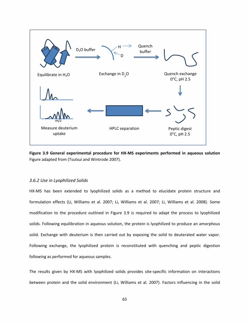
65
Figure 3.9 General experimental procedure for HX-MS experiments performed in aqueous solution
Figure adapted from (Tsutsui and Wintrode 2007).
3.6.2 Use in Lyophilized Solids
HX-MS has been extended to lyophilized solids as a method to elucidate protein structure and
formulation effects (Li, Williams et al. 2007; Li, Williams et al. 2007; Li, Williams et al. 2008). Some
modification to the procedure outlined in Figure 3.9 is required to adapt the process to lyophilized
solids. Following equilibration in aqueous solution, the protein is lyophilized to produce an amorphous
solid. Exchange with deuterium is then carried out by exposing the solid to deuterated water vapor.
Following exchange, the lyophilized protein is reconstituted with quenching and peptic digestion
following as performed for aqueous samples.
The results given by HX-MS with lyophilized solids provides site-specific information on interactions
between protein and the solid environment (Li, Williams et al. 2007). Factors influencing in the solid
Equilibrate in H2O
H
D
Exchange in D2O
D2O buffer
Quench exchange 0°C, pH 2.5
Peptic digest 0°C, pH 2.5
Quench buffer
m/z
HPLC separation Measure deuterium uptake

66
state include relative humidity during exchange, inclusion of salts and inclusion of stabilizing excipients
(Li, Williams et al. 2007; Li, Williams et al. 2007). HX-MS with lyophilized proteins provides a quantitative
and site-specific tool for the study of protein-excipient interactions in amorphous solids.

67
4.0 PROPERTY MODEL DEVELOPMENT: THE FORWARD PROBLEM
CAMD requires accurate and predictive property models for design or selection of candidate molecules.
For development of property models, molecular descriptors are needed for correlation between
molecular structure and properties of interest. For example, an overview of the experimental procedure
and model development steps in the design of lyophilized protein formulation is given by Figure 4.1 with
the steps relevant to property model development highlighted.
The property models considered here are classified either as quantitative structure-property
relationships (QSPRs), group contribution (GC) methods or thermodynamic property models. The
property models developed here are given in Table 4.1, along with the corresponding descriptor type
and model type. Additional property models available in literature were used where applicable.
The types of molecular descriptors used are discussed in Section 4.1. Development of linear QSPRs is
described in Section 4.2 and development of non-linear QSPRs is described in Section 4.3. Group
contribution methods are detailed in Section 4.4. Finally, the development of a UNIFAC thermodynamic
property model for ionic liquids (UNIFAC-IL) is outlined in Section 4.5.
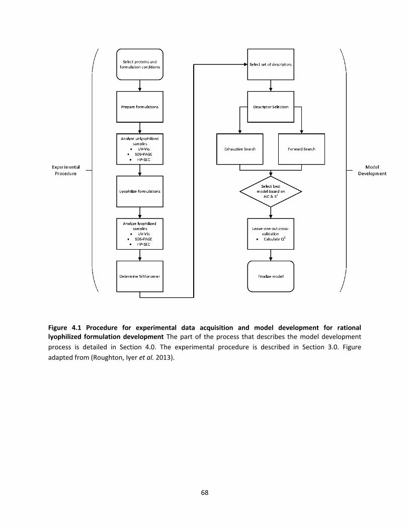
68
Figure 4.1 Procedure for experimental data acquisition and model development for rational lyophilized formulation development The part of the process that describes the model development
process is detailed in Section 4.0. The experimental procedure is described in Section 3.0. Figure
adapted from (Roughton, Iyer et al. 2013).
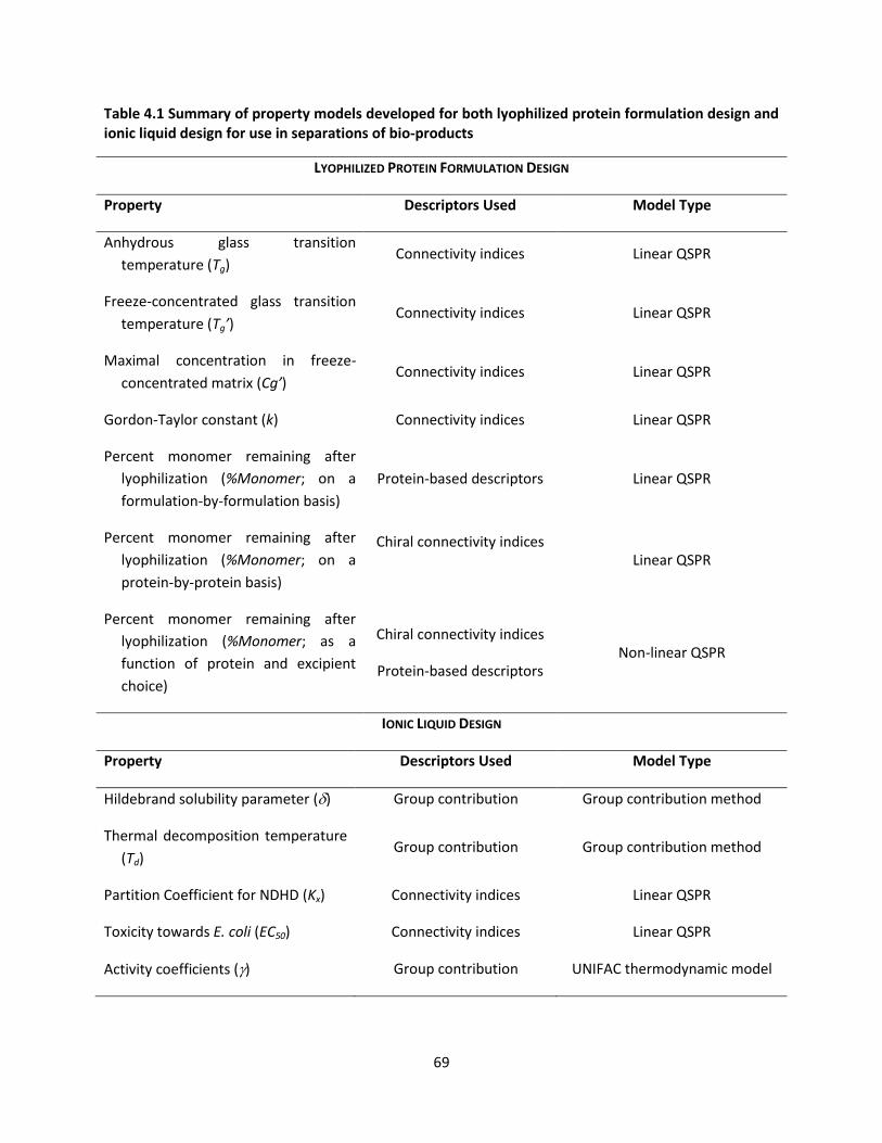
69
Table 4.1 Summary of property models developed for both lyophilized protein formulation design and ionic liquid design for use in separations of bio-products
LYOPHILIZED PROTEIN FORMULATION DESIGN
Property Descriptors Used Model Type
Anhydrous glass transition
temperature (Tg) Connectivity indices Linear QSPR
Freeze-concentrated glass transition
temperature (Tg’) Connectivity indices Linear QSPR
Maximal concentration in freeze-
concentrated matrix (Cg’) Connectivity indices Linear QSPR
Gordon-Taylor constant (k) Connectivity indices Linear QSPR
Percent monomer remaining after
lyophilization (%Monomer; on a
formulation-by-formulation basis)
Protein-based descriptors Linear QSPR
Percent monomer remaining after
lyophilization (%Monomer; on a
protein-by-protein basis)
Chiral connectivity indices
Linear QSPR
Percent monomer remaining after
lyophilization (%Monomer; as a
function of protein and excipient
choice)
Chiral connectivity indices
Protein-based descriptors Non-linear QSPR
IONIC LIQUID DESIGN
Property Descriptors Used Model Type
Hildebrand solubility parameter () Group contribution Group contribution method
Thermal decomposition temperature
(Td) Group contribution Group contribution method
Partition Coefficient for NDHD (Kx) Connectivity indices Linear QSPR
Toxicity towards E. coli (EC50) Connectivity indices Linear QSPR
Activity coefficients () Group contribution UNIFAC thermodynamic model
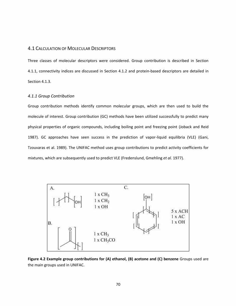
70
4.1 CALCULATION OF MOLECULAR DESCRIPTORS
Three classes of molecular descriptors were considered. Group contribution is described in Section
4.1.1, connectivity indices are discussed in Section 4.1.2 and protein-based descriptors are detailed in
Section 4.1.3.
4.1.1 Group Contribution
Group contribution methods identify common molecular groups, which are then used to build the
molecule of interest. Group contribution (GC) methods have been utilized successfully to predict many
physical properties of organic compounds, including boiling point and freezing point (Joback and Reid
1987). GC approaches have seen success in the prediction of vapor-liquid equilibria (VLE) (Gani,
Tzouvaras et al. 1989). The UNIFAC method uses group contributions to predict activity coefficients for
mixtures, which are subsequently used to predict VLE (Fredenslund, Gmehling et al. 1977).
Figure 4.2 Example group contributions for (A) ethanol, (B) acetone and (C) benzene Groups used are
the main groups used in UNIFAC.

71
In general, groups are determined by the author of the method and can vary from method to method.
An example of the groups present in several molecules as defined by UNIFAC is given by Figure 4.2. As
every chemical group needs to be accounted for, descriptor selection methods (cf. Section 4.2.4) cannot
be utilized in the development of GC methods. The motivation behind group contributions is that results
from a limited experimental data set can be applied to other systems with different molecule structures,
but the same basic molecular groups. One major limitation of GC methods is that they cannot account
for groups that are not present in the model-building set. GC methods assume that the number of a
certain group present and the location of groups within a molecule do not affect the observed property
of the molecule (Prausnitz, Lichtenthaler et al. 1999). This assumption is incorrect; improvement can
come with the definition of more groups or higher-order groups, albeit with the need for more model
parameters (Prausnitz, Lichtenthaler et al. 1999; Harper and Gani 2000). Predictions from GC methods
offer a first approximation for properties (Prausnitz, Lichtenthaler et al. 1999) and are thus useful for
property screening purposes (Gani, Nielsen et al. 1991).
4.1.2 Connectivity Indices
Topological descriptors are a class of molecular descriptors which identify individual atoms and their
bonding configuration in a molecule. Connectivity indices are a type of topological descriptors first
proposed by Randic (1975). Later work extended the use of connectivity indices to pharmaceutical
product property prediction (Kier and Hall 1986) and polymer property prediction (Bicerano 2002). The
use of connectivity indices have been proposed to describe missing groups for GC models (Gani, Harper
et al. 2005; Satyanarayana, Abildskov et al. 2009).
Connectivity indices were chosen as the class of excipient descriptors to be used in model development.
Connectivity indices were also used for some ionic liquid property models where group contribution did
not perform with acceptable accuracy. Connectivity indices have utility due to the ability to calculate
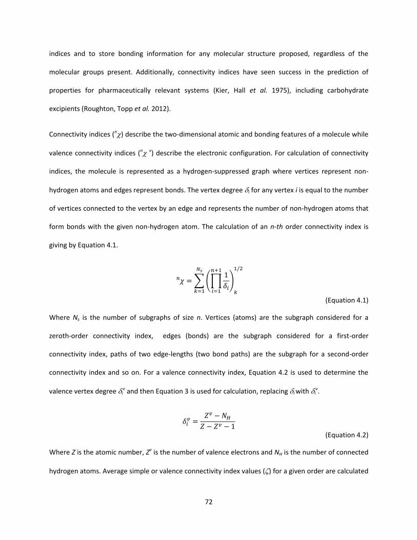
72
indices and to store bonding information for any molecular structure proposed, regardless of the
molecular groups present. Additionally, connectivity indices have seen success in the prediction of
properties for pharmaceutically relevant systems (Kier, Hall et al. 1975), including carbohydrate
excipients (Roughton, Topp et al. 2012).
Connectivity indices (n) describe the two-dimensional atomic and bonding features of a molecule while
valence connectivity indices (n v) describe the electronic configuration. For calculation of connectivity
indices, the molecule is represented as a hydrogen-suppressed graph where vertices represent non-
hydrogen atoms and edges represent bonds. The vertex degree i for any vertex i is equal to the number
of vertices connected to the vertex by an edge and represents the number of non-hydrogen atoms that
form bonds with the given non-hydrogen atom. The calculation of an n-th order connectivity index is
giving by Equation 4.1.
∑ (∏
)
(Equation 4.1)
Where Ns is the number of subgraphs of size n. Vertices (atoms) are the subgraph considered for a
zeroth-order connectivity index, edges (bonds) are the subgraph considered for a first-order
connectivity index, paths of two edge-lengths (two bond paths) are the subgraph for a second-order
connectivity index and so on. For a valence connectivity index, Equation 4.2 is used to determine the
valence vertex degree iv and then Equation 3 is used for calculation, replacing i with i
v.
(Equation 4.2)
Where Z is the atomic number, Zv is the number of valence electrons and NH is the number of connected
hydrogen atoms. Average simple or valence connectivity index values () for a given order are calculated
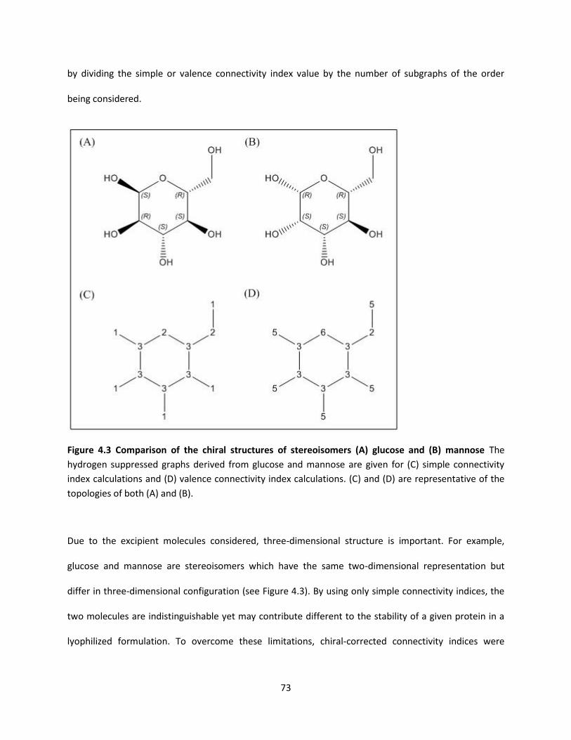
73
by dividing the simple or valence connectivity index value by the number of subgraphs of the order
being considered.
Figure 4.3 Comparison of the chiral structures of stereoisomers (A) glucose and (B) mannose The
hydrogen suppressed graphs derived from glucose and mannose are given for (C) simple connectivity
index calculations and (D) valence connectivity index calculations. (C) and (D) are representative of the
topologies of both (A) and (B).
Due to the excipient molecules considered, three-dimensional structure is important. For example,
glucose and mannose are stereoisomers which have the same two-dimensional representation but
differ in three-dimensional configuration (see Figure 4.3). By using only simple connectivity indices, the
two molecules are indistinguishable yet may contribute different to the stability of a given protein in a
lyophilized formulation. To overcome these limitations, chiral-corrected connectivity indices were
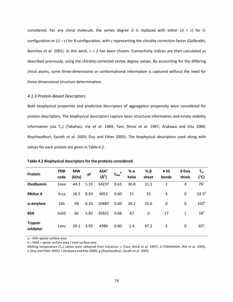
74
considered. For any chiral molecule, the vertex degree i is replaced with either (i + c) for S-
configuration or (i – c) for R-configuration, with c representing the chirality correction factor (Golbraikh,
Bonchev et al. 2001). In this work, c = 2 has been chosen. Connectivity indices are then calculated as
described previously, using the chirality-corrected vertex degree values. By accounting for the differing
chiral atoms, some three-dimensional or conformational information is captured without the need for
three-dimensional structure determination.
4.1.3 Protein-Based Descriptors
Both biophysical properties and predictive descriptors of aggregation propensity were considered for
protein descriptors. The biophysical descriptors capture basic structural information and innate stability
information (via Tm) (Takahasi, Irie et al. 1969; Tani, Shirai et al. 1997; Arakawa and Kita 2000;
Roychaudhuri, Sarath et al. 2003; Duy and Fitter 2005). The biophysical descriptors used along with
values for each protein are given in Table 4.2.
Table 4.2 Biophysical descriptors for the proteins considered
Protein PDB
code
MW
(kDa) pI
ASAa
(Å2) fASA
b % α
helix
% β
sheet
# SS
bonds
# free
thiols
Tm
(°C)
Ovalbumin 1ova 44.3 5.19 34237 0.63 30.8 31.3 1 4 76c
RNAse A 5rsa 16.5 8.93 4052 0.60 21 33 4 0 62.5d
α-amylase 1bli 58 6.33 10480 0.60 26.2 25.6 0 0 102e
BSA 3v03 66 5.82 35921 0.68 67 0 17 1 59f
Trypsin
inhibitor 1avu 20.1 4.95 4986 0.60 1.4 97.2 2 0 65g
a – ASA=apolar surface area b – fASA = apolar surface area / total surface area Melting temperature (Tm) values were obtained from literature: c (Tani, Shirai et al. 1997), d (TAKAHASHI, IRIE et al. 1969), e (Duy and Fitter 2005), f (Arakawa and Kita 2000), g (Roychaudhuri, Sarath et al. 2003)

75
Descriptors calculated from two primary sequence-based methods for the prediction of aggregation
propensity were also considered: AGGRESCAN (Conchillo-Sole, de Groot et al. 2007) and PASTA (Trovato,
Chiti et al. 2006; Trovato, Seno et al. 2007). Both methods require only the amino acid sequence and
offer web-based servers for calculation of all relevant variables (AGGRESCAN: bioinf.uab.es/aggrescan/
and PASTA: http://biocomp.bio.unipd.it/pasta/). AGGRESCAN predicts aggregation propensity by
determining “hot spots” or short amino acid sequences that are likely to be aggregation-prone. PASTA
predicts aggregation propensity by determining sequences that are likely to induce aggregation through
the formation of intermolecular -strands. Both methods are primarily concerned with amyloid fibril
formation. Explanation of the descriptors calculated or derived from these methods is given in Table 4.3.
Table 4.3 Descriptors obtained and derived from aggregation propensity prediction methods
AGGRESCAN Descriptor Name Definition
a3vSA Sequence average amino acid aggregation propensity
nHS Number of aggregation hot spots
NnHS nHS normalized by number of residues in protein
AAT Area of aggregation profile above hot spot threshold
THSA Total area of aggregation profile comprising hot spots
TA Total area of aggregation profile
AATr AAT normalized by number of residues in protein
THSAr THSA normalized by number of residues in protein
Na4vSS Sliding window average of amino acid propensity values divided
by number of amino acids in protein
PASTA Descriptor Name
Emin Minimum energy of PASTA pairings
Eavg Average energy of PASTA pairings
Lmax Average amino acid pair length of PASTA pairings
Lavg Maximum amino acid pair length of PASTA pairings
(E/L)min Minimum ratio of energy to length of PASTA pairings
(E/L)avg Average ratio of energy to length of PASTA pairings
# of Peaks Number of peaks in PASTA aggregation profile
4.1.4 Principal Component Analysis
76
Principal component analysis (PCA) is a data-reduction technique which replaces an original set of
variables with a smaller number of principal components, which are calculated through linear
combinations of the original variables (Maindonald and Braun 2010). Through development of principal
components, the majority of variance in the data set is captured with a minimal number of variables. In
this work, PCA was used to visualize the excipient descriptor space. Such visualization is used for the
discussion of results. PCA was performed using the DAAG package in R (Maindonald and Braun 2010).
4.2 DEVELOPMENT OF LINEAR QSPRS
Development of linear QSPRs is comprised of four steps:
1. Identification of key properties and procurement of experimental property values
2. Calculation of descriptors and descriptor selection
3. Linear regression
4. Cross-validation
The steps are further detailed in the following sections.
4.2.1 Glass Transition Properties
QSPRs were developed for the glass transition temperature of the anhydrous solute, glass transition
temperature of the maximally concentrated solute, melting point of ice and Gordon-Taylor constant for
carbohydrates. The experimental data were collected from published literature(Roos 1993). Discussion
on glass transitions and their importance in lyophilized protein formulations is given in detail in Section
2.5.
4.2.2 Percent Monomer Remaining Following Lyophilization
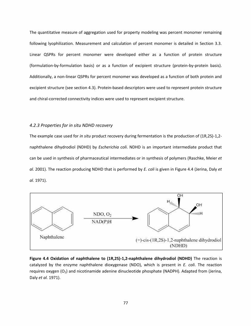
77
The quantitative measure of aggregation used for property modeling was percent monomer remaining
following lyophilization. Measurement and calculation of percent monomer is detailed in Section 3.3.
Linear QSPRs for percent monomer were developed either as a function of protein structure
(formulation-by-formulation basis) or as a function of excipient structure (protein-by-protein basis).
Additionally, a non-linear QSPRs for percent monomer was developed as a function of both protein and
excipient structure (see section 4.3). Protein-based descriptors were used to represent protein structure
and chiral-corrected connectivity indices were used to represent excipient structure.
4.2.3 Properties for in situ NDHD recovery
The example case used for in situ product recovery during fermentation is the production of (1R,2S)-1,2-
naphthalene dihydrodiol (NDHD) by Escherichia coli. NDHD is an important intermediate product that
can be used in synthesis of pharmaceutical intermediates or in synthesis of polymers (Raschke, Meier et
al. 2001). The reaction producing NDHD that is performed by E. coli is given in Figure 4.4 (Jerina, Daly et
al. 1971).
Figure 4.4 Oxidation of naphthalene to (1R,2S)-1,2-naphthalene dihydrodiol (NDHD) The reaction is
catalyzed by the enzyme naphthalene dioxygenase (NDO), which is present in E. coli. The reaction
requires oxygen (O2) and nicotinamide adenine dinucleotide phosphate (NADPH). Adapted from (Jerina,
Daly et al. 1971).
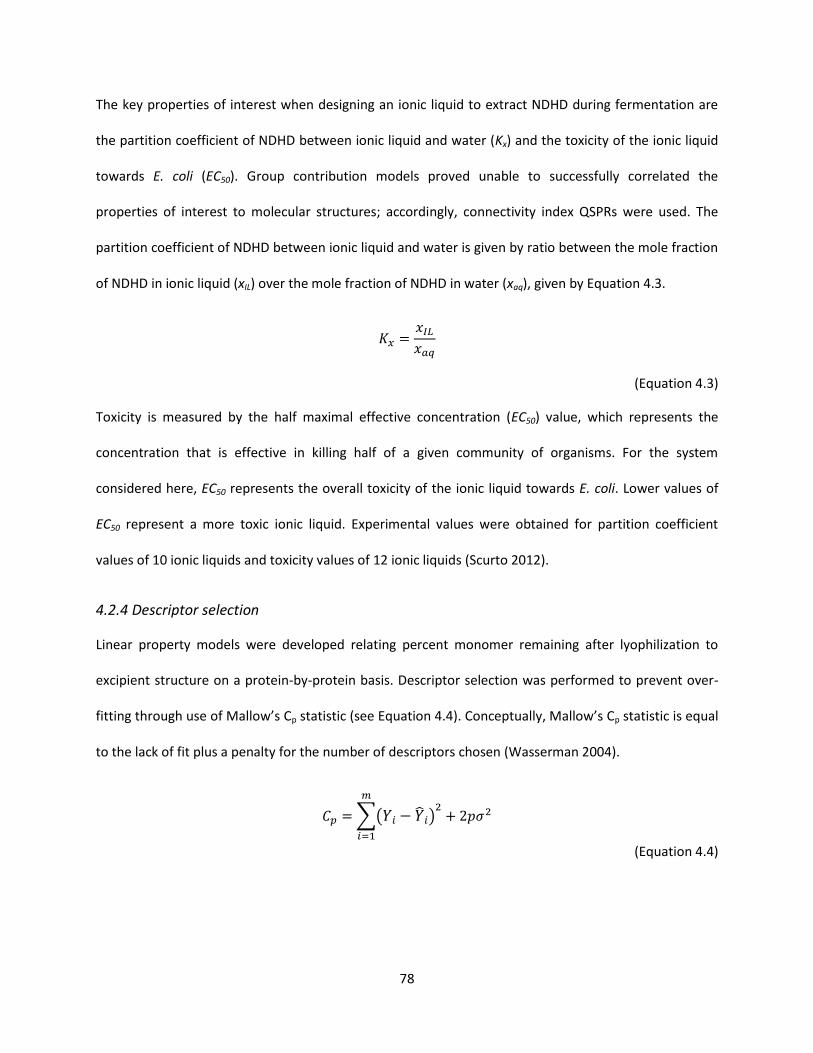
78
The key properties of interest when designing an ionic liquid to extract NDHD during fermentation are
the partition coefficient of NDHD between ionic liquid and water (Kx) and the toxicity of the ionic liquid
towards E. coli (EC50). Group contribution models proved unable to successfully correlated the
properties of interest to molecular structures; accordingly, connectivity index QSPRs were used. The
partition coefficient of NDHD between ionic liquid and water is given by ratio between the mole fraction
of NDHD in ionic liquid (xIL) over the mole fraction of NDHD in water (xaq), given by Equation 4.3.
(Equation 4.3)
Toxicity is measured by the half maximal effective concentration (EC50) value, which represents the
concentration that is effective in killing half of a given community of organisms. For the system
considered here, EC50 represents the overall toxicity of the ionic liquid towards E. coli. Lower values of
EC50 represent a more toxic ionic liquid. Experimental values were obtained for partition coefficient
values of 10 ionic liquids and toxicity values of 12 ionic liquids (Scurto 2012).
4.2.4 Descriptor selection
Linear property models were developed relating percent monomer remaining after lyophilization to
excipient structure on a protein-by-protein basis. Descriptor selection was performed to prevent over-
fitting through use of Mallow’s Cp statistic (see Equation 4.4). Conceptually, Mallow’s Cp statistic is equal
to the lack of fit plus a penalty for the number of descriptors chosen (Wasserman 2004).
∑( )
(Equation 4.4)
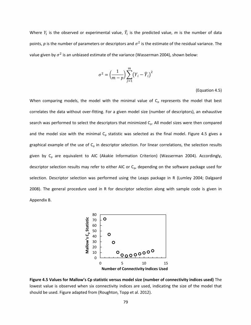
79
Where is the observed or experimental value, is the predicted value, m is the number of data
points, p is the number of parameters or descriptors and is the estimate of the residual variance. The
value given by is an unbiased estimate of the variance (Wasserman 2004), shown below:
(
)∑( )
(Equation 4.5)
When comparing models, the model with the minimal value of Cp represents the model that best
correlates the data without over-fitting. For a given model size (number of descriptors), an exhaustive
search was performed to select the descriptors that minimized Cp. All model sizes were then compared
and the model size with the minimal Cp statistic was selected as the final model. Figure 4.5 gives a
graphical example of the use of Cp in descriptor selection. For linear correlations, the selection results
given by Cp are equivalent to AIC (Akakie Information Criterion) (Wasserman 2004). Accordingly,
descriptor selection results may refer to either AIC or Cp, depending on the software package used for
selection. Descriptor selection was performed using the Leaps package in R (Lumley 2004; Dalgaard
2008). The general procedure used in R for descriptor selection along with sample code is given in
Appendix B.
Figure 4.5 Values for Mallow’s Cp statistic versus model size (number of connectivity indices used) The
lowest value is observed when six connectivity indices are used, indicating the size of the model that
should be used. Figure adapted from (Roughton, Topp et al. 2012).
0
10
20
30
40
50
60
70
80
0 5 10 15
Mal
low
's C
p S
tati
stic
Number of Connectivity Indices Used
80
4.2.5 Cross-Validation
Once a final model was selected, leave-one-out cross-validation (LOOCV) was performed to evaluate the
predictive ability of the model. In LOOCV, one by one, each observation is left out of the data set and
then the selected descriptors are again correlated to the data set. The resulting model is then used to
predict the left-out data point. The process is repeated for each fold. Upon completion, the predictions
are used to calculate the predicted residual sum of the square errors (PRESS) through use of Equation
4.6 (Quan 1988).
∑( ⟨ ⟩)
(Equation 4.6)
where ⟨ ⟩ is the predicted value for the left-out observation and m is the total number of observations.
The PRESS value is then used to calculate the cross-validation coefficient Q2 (see Equation 4.7).
∑ ( )
(Equation 4.7)
where is the average value for all data points. Q2 has a maximal value of the model’s R2 value, which
represents a perfect predictive ability (Quan 1988). When comparing models, smaller R2-Q2 values
represent better predictive power. In general, Q2 can be calculated for K-fold cross-validation by
expanding upon Equation 4.6 to yield Equation 4.8. In K-fold cross-validation, K number of folds are
generated from the original data set. The number of data left-out should be equal for each fold. As K
decreases, the predictive power of the model is further strained as fewer observations are used to build
the model.

81
∑∑( ⟨ ⟩)
(Equation 4.8)
where k is the number of folds and n is the number of observations left-out in each fold. The general
procedure used in R for cross-validation along with sample code is given in Appendix B.
4.3 DEVELOPMENT OF NON-LINEAR QSPRS
A non-linear QSPR was used to describe percent monomer remaining after lyophilization as a function of
both protein and excipient choice. More details concerning percent monomer remaining after
lyophilization can be found in Section 4.2.2. Development of non-linear QSPRs offer an added layer of
complexity in comparison to linear QSPR development as a functional form must first be selected, where
the functional form is assumed in linear QSPR development. Additionally, certain assumptions in the
development of linear correlations do not hold for non-linear correlations.
4.3.1 Selection of Functional Forms
Several functional forms for a model describing protein stability following lyophilization as a function of
excipient choice and protein choice were considered. Attempts to build a linear model of sufficient
correlative quality were unsuccessful (results not shown). Non-linear models were considered to better
correlate the descriptors to the %Monomer values. The final form used is given below:
(∑ ) (∑ )
(Equation 4.9)
where represents excipient descriptors, represents protein descriptors, and a, b, and c are
adjustable parameters.

82
The form used for Equation 4.9 was motivated by the enthalpic contribution to the Flory-Huggins model,
given by Equation 4.10. The Flory-Huggins model has been used previously to describe protein-sugar
interactions in lyophilized solids (Katayama, Carpenter et al. 2009; Wang, Tchessalov et al. 2009).
Equation 4.9 emulates the Flory-Huggins interaction parameter (12) through the multiplication of
excipient structural descriptors and protein structural descriptors. The success of the Flory-Huggins
functional form of the universal model suggests that direct protein-excipient interactions play a
significant role in stabilization of the protein during lyophilization for the formulations considered.
(Equation 4.10)
4.3.2 Parameter Fitting
A non-linear model was considered for the correlation between percent monomer remaining after
lyophilization and both excipient and protein descriptors, referred to as the universal model. Parameter
fitting was performed by minimization of the residual sum of the squares (RSS) between the model and
experimental data. The minimization was performed as a mixed-integer non-linear program (MINLP),
resulting in parameter values that were not guaranteed to be globally optimal. However, the
formulation of the problem as a MINLP is necessary as a non-linear property model is used for the
universal model. The Excel solver was utilized in solution of the MINLP.
4.3.3 Parameter Sensitivity
A parameter sensitivity analysis was used to select descriptors. Given the functional form, all descriptors
were included. The parameters for each descriptor were determined such that the residual sum of the
squares (RSS) between the model and experimental data was minimized (see Section 4.3.2). Sensitivity
(Sx) was then calculated descriptor by descriptor through use of Equation 4.11.

83
(Equation 4.11)
Where RSS1.1*x represents the sum of the square errors after increasing the parameter value for a given
descriptor (x) by a factor of 1.1. When Sx is equal to or near one, the descriptor in question had no
discernible effect on the model outcome. Larger sensitivities suggest a stronger importance on model
outcome for the descriptor of interest. Sensitivity values were used to guide two rounds of descriptor
selection. In the first round of descriptor reduction, descriptors with sensitivities approximately equal to
one were excluded. In the second round of descriptor reduction, the remaining descriptor with the
lowest sensitivity was excluded from the model and parameter fitting through minimization of RSS was
redone for the remaining descriptors. If the model performance statistics changed by less than an order
of magnitude, the descriptor remained excluded; otherwise the descriptor was retained in the final
model. The procedure was repeated for the descriptor with the next lowest sensitivity value until all
descriptors had been considered.
4.3.4 Statistical Verification
The model performance statistics of interest were the percent average absolute deviation (%AAD) and
the reduced chi-squared value. The statistics were used for the non-linear model over R2 and Q2 as R2-
based methods are poor indicators of non-linear model performance (Spiess and Neumeyer 2010).
Furthermore, calculation of R2 assumes that the total sum of squares is equal to the explained sum of
squares plus the residual sum of squares (TSS = ESS + RSS). The assumption is valid for linear regression
but does not hold for non-linear regression. The %AAD gives the average deviation between the
experimental and the predicted values given by the model (see Equation 4.12). %AAD was used to
evaluate the accuracy of the model.
84
∑| |
(Equation 4.12)
The predictive power of the model was evaluated using reduced chi-squared. The reduced chi-squared
statistic accounts for model variance as well as the number of parameters chosen (see Equation 4.13).
For each data point, the difference between experimental and predicted is normalized by the
uncertainty of the experimental measurement (). A value of one indicates that the model provides a
good fit for the data, as the model variance is equal to the experimental variance (Spiess and Neumeyer
2010). Order of magnitude differences in reduced chi-squared value suggest that either measurement
errors are over-estimated (reduced chi-squared < 0.1) or a combination of under-estimated
measurement errors and incorrect choice of functional form for the model (reduced chi-squared > 10)
(Spiess and Neumeyer 2010).
reduced chi-squared
∑
( )
(Equation 4.13)
4.4 GROUP CONTRIBUTION METHODS
For design of IL-based separation processes, group contribution (GC) models for heat capacity (Gardas
and Coutinho 2008) and density (Valderrama and Robles 2007) were required. A solubility parameter GC
model was developed for use as a design target and ionic liquid selection criteria. Additionally, a thermal
decomposition temperature GC model was developed for use in selection of ionic liquid candidates.
4.4.1 Hildebrand Solubility Parameter
The Hildebrand solubility parameter is used to predict whether compounds will be miscible (Barton
1991). Compounds with similar solubility parameter values are more likely to form a miscible solution.
Solubility is a key parameter for selecting an entrainer, allowing the solubility parameter to be used as a
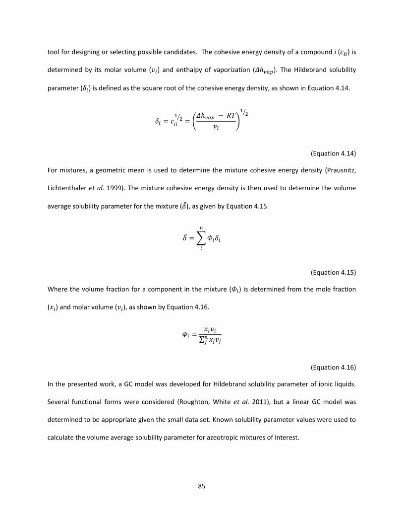
85
tool for designing or selecting possible candidates. The cohesive energy density of a compound i ( ) is
determined by its molar volume ( ) and enthalpy of vaporization ( ). The Hildebrand solubility
parameter ( ) is defined as the square root of the cohesive energy density, as shown in Equation 4.14.
⁄ (
)
⁄
(Equation 4.14)
For mixtures, a geometric mean is used to determine the mixture cohesive energy density (Prausnitz,
Lichtenthaler et al. 1999). The mixture cohesive energy density is then used to determine the volume
average solubility parameter for the mixture ( ), as given by Equation 4.15.
∑
(Equation 4.15)
Where the volume fraction for a component in the mixture ( ) is determined from the mole fraction
( ) and molar volume ( ), as shown by Equation 4.16.
∑
(Equation 4.16)
In the presented work, a GC model was developed for Hildebrand solubility parameter of ionic liquids.
Several functional forms were considered (Roughton, White et al. 2011), but a linear GC model was
determined to be appropriate given the small data set. Known solubility parameter values were used to
calculate the volume average solubility parameter for azeotropic mixtures of interest.
86
4.4.2 Thermal Decomposition Temperature
An important consideration of the design or selection of an ionic liquid for a separations process is the
thermal decomposition temperature. Temperatures under 500°C have been reported to lead to thermal
decomposition of the alkyl chain substituents of the cation as well as the anion itself (Ohtani, Ishimura
et al. 2008). Higher temperatures (>500°C) can result in thermal decomposition of the imidazolium ring
in cations (Ohtani, Ishimura et al. 2008). Imidazolium-based cations generally exhibit higher thermal
stability than other cation types, such as tetraalkyl ammonium-based cations (Ngo, LeCompte et al.
2000). Operating temperatures for any process utilizing ionic liquids must be well below the thermal
degradation onset temperature of the ionic liquids.
4.4.3 Group Contribution Model Development
Group contribution models were developed to predict solubility parameters and thermal decomposition
temperature for ionic liquids to provide a screening tool for selection of ionic liquids for use as
entrainers. Additionally, group contributions form the basis of the activity coefficient predictions from
the UNIFAC model (see Section 4.5). The ionic liquids were characterized as alkyl chain groups, cation
groups, and anion groups. The groups used to develop ionic liquid GC models are given by Table 4.4.

87
Table 4.4 Ionic liquid groups used for GC model development Groups are classified either as alkyl chain
groups, cation groups or anion groups. The X represents a point of connection with another group.
Hildebrand solubility parameter and Td = thermal decomposition temperature.
Alkyl Chain Groups
Name Structure Models
CH3
, Td,
UNIFAC
CH2
, Td,
UNIFAC
O (ether)
Isobutyl
Td
Ethylbenzyl
Td
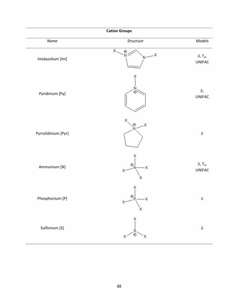
88
Cation Groups
Name Structure Models
Imidazolium [Im]
, Td,
UNIFAC
Pyridinium [Py]
,
UNIFAC
Pyrrolidinium [Pyr]
Ammonium [N]
, Td,
UNIFAC
Phosphonium [P]
Sulfonium [S]

89
Anion Groups
Name Structure Models
Dimethylphosphate [DMP]
,
UNIFAC
Diethylphosphate [DEP]
Tetrafluoroborate [BF4]
, Td,
UNIFAC
Hexafluorophosphate [PF6]
, Td,
UNIFAC
Trifluoroacetate [CF3COO]
, Td,
UNIFAC
Trifluoromethanesulfonate
[CF3SO3]
, Td,
UNIFAC

90
Bis(trifluoromethylsulfonyl)
amide [Tf2N]
, Td,
UNIFAC
2-(2-methoxyethoxy)ethyl
sulfate [CH3(OC2H4)2SO4]
,
UNIFAC
2-(methoxy)ethyl sulfate
[CH3OC2H4SO4]
UNIFAC
2-(ethoxy)ethyl sulfate
[C2H5OC2H4SO4]
UNIFAC
Methyl sulfate [CH3SO4]
UNIFAC
Ethyl sulfate [C2H5SO4]
UNIFAC
Octyl sulfate [C8H17SO4]
Thiocyanate [SCN]
,
UNIFAC

91
Tosylate [TOS]
Chloride [Cl]
, Td,
UNIFAC
Bromide [Br]
Td,
UNIFAC
Iodide [I]
UNIFAC
Linear models were proposed to predict the solubility parameter and thermal decomposition
temperature. The function form for prediction of property P is given by Equation 4.17, where
describes the number of groups of type i, is the contribution of group i to the overall property value,
and b is a constant. The contributions from the alkyl chain groups, cation groups, and anion groups are
summed to give the predicted property value. The function forms used in the UNIFAC model differ and
are explained in Section 4.5.
∑
∑
∑
(Equation 4.17)
Experimental values of ionic liquid solubility parameters were obtained from literature (Marciniak 2010).
The solubility parameter value can change with temperature, so the model was developed to predict the
solubility parameter at 298.15 K. Even though a temperature dependence exists, solubility parameter
often scales linearly for all compounds (Barton 1991). Thus, the GC model developed can be utilized to
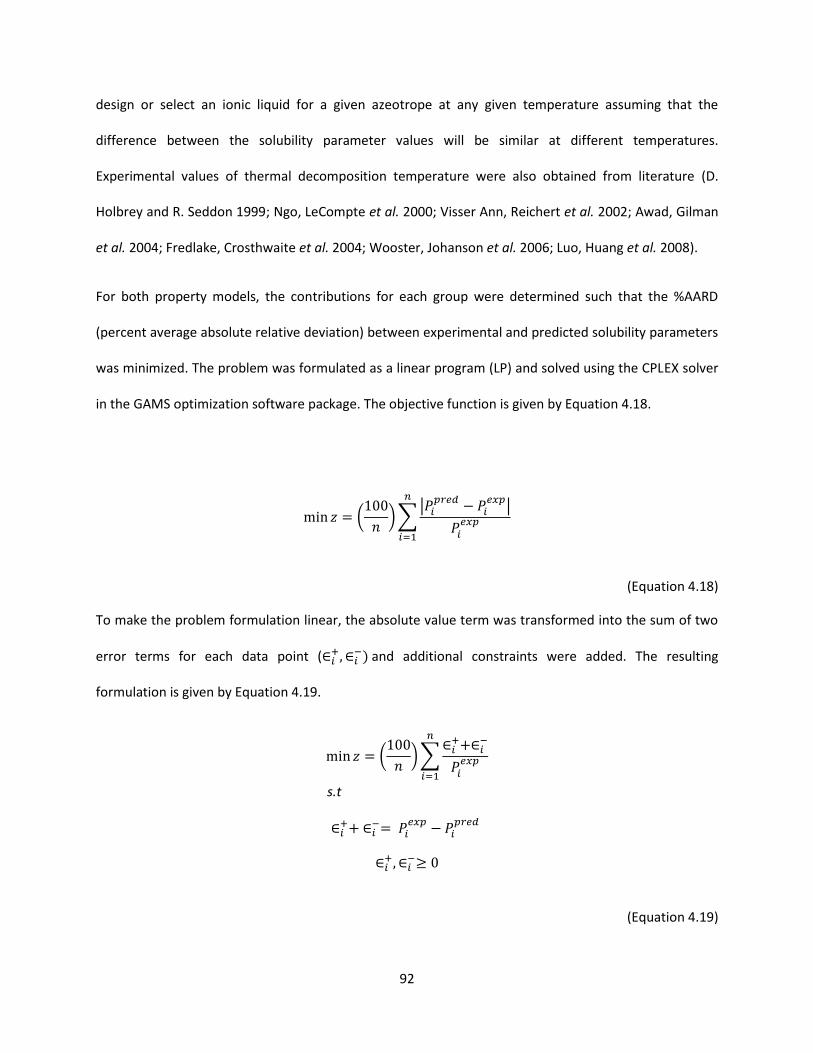
92
design or select an ionic liquid for a given azeotrope at any given temperature assuming that the
difference between the solubility parameter values will be similar at different temperatures.
Experimental values of thermal decomposition temperature were also obtained from literature (D.
Holbrey and R. Seddon 1999; Ngo, LeCompte et al. 2000; Visser Ann, Reichert et al. 2002; Awad, Gilman
et al. 2004; Fredlake, Crosthwaite et al. 2004; Wooster, Johanson et al. 2006; Luo, Huang et al. 2008).
For both property models, the contributions for each group were determined such that the %AARD
(percent average absolute relative deviation) between experimental and predicted solubility parameters
was minimized. The problem was formulated as a linear program (LP) and solved using the CPLEX solver
in the GAMS optimization software package. The objective function is given by Equation 4.18.
(
)∑
|
|
(Equation 4.18)
To make the problem formulation linear, the absolute value term was transformed into the sum of two
error terms for each data point (
) and additional constraints were added. The resulting
formulation is given by Equation 4.19.
(
)∑
s.t
(Equation 4.19)

93
4.5 UNIFAC-IL MODEL DEVELOPMENT
Design of separations requires the determination of thermodynamic parameters for all components
involved in the separation. For the design of extractive distillation processes, the activity coefficient is
needed for the light components, heavy components and the entrainers. A UNIFAC model was
developed to predict ionic liquid activity coefficients (UNIFAC-IL). Known UNIFAC parameters were used
for light and heavy components.
4.5.1 Theory
Modeling or prediction of VLE is a key tool needed for the design of separation processes. For the
examples considered, the pressure was near or at atmosphere and the vapor phase was considered
ideal. The Poynting correction was neglected and the saturated fugacity coefficients were assumed to be
unity, also due to low pressure. Due to the extremely low vapor pressure exhibited by ionic liquids, the
saturation pressure ( ) for the ionic liquids was assumed to be zero. As a result, no ionic liquid was
assumed to be present in the vapor phase. Factoring in the assumptions, total pressure for a ternary
system containing an ionic liquid is given by Equation 4.20, where components (1) and (2) are not ionic
liquids.
(Equation 4.20)
Given a known total pressure, the vapor compositions for component (1) or (2) are given by Equation
4.21.
(Equation 4.21)
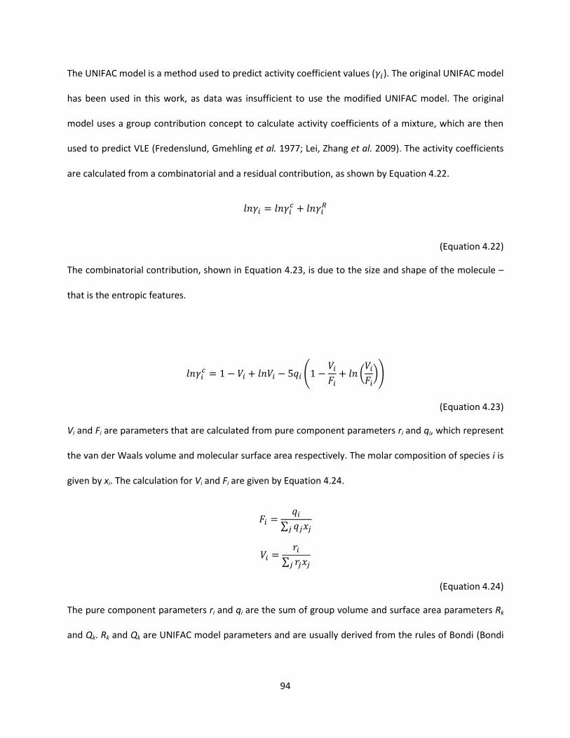
94
The UNIFAC model is a method used to predict activity coefficient values ( ). The original UNIFAC model
has been used in this work, as data was insufficient to use the modified UNIFAC model. The original
model uses a group contribution concept to calculate activity coefficients of a mixture, which are then
used to predict VLE (Fredenslund, Gmehling et al. 1977; Lei, Zhang et al. 2009). The activity coefficients
are calculated from a combinatorial and a residual contribution, as shown by Equation 4.22.
(Equation 4.22)
The combinatorial contribution, shown in Equation 4.23, is due to the size and shape of the molecule –
that is the entropic features.
(
(
))
(Equation 4.23)
Vi and Fi are parameters that are calculated from pure component parameters ri and qi, which represent
the van der Waals volume and molecular surface area respectively. The molar composition of species i is
given by xi. The calculation for Vi and Fi are given by Equation 4.24.
∑
∑
(Equation 4.24)
The pure component parameters ri and qi are the sum of group volume and surface area parameters Rk
and Qk. Rk and Qk are UNIFAC model parameters and are usually derived from the rules of Bondi (Bondi

95
1964). Calculation of the parameters is given by Equation 4.25, with vk(i) representing the number of
groups of type k present in molecule i.
∑ ( )
∑ ( )
(Equation 4.25)
The residual contribution, shown in Equation 4.26, accounts for the interactions between groups – that
is the enthalpic contribution.
∑
( )
[ ( )
]
(Equation 4.26)
The group residual activity coefficient is given by k (see Equation 4.27), where k (i) represents residual
activity coefficient of group k in a reference solution containing only molecules of type i.
[ (∑
) ∑(
∑ )
]
(Equation 4.27)
m is a volume contribution parameter and is dependent on Xm, which is the fraction of group m in the
given mixture. Calculation of m and Xm is given by Equation 4.28.
∑
∑
( )
∑ ∑ ( )
(Equation 4.28)

96
The interaction parameter nm (see Equation 4.29) is a function of the group interaction parameter anm
and temperature (T). The group interaction parameter anm is a fitted UNIFAC model parameter with the
property that anm ≠ amn.
(
)
(Equation 4.29)
4.5.2 Determination of Groups and Group Parameters
The ionic liquids were characterized by the same groups as used for the solubility parameter: alkyl chain
groups, cation groups, and anion groups. Previous attempts to develop a UNIFAC model for ionic liquids
characterized a cation and anion pair as one group (Lei, Zhang et al. 2009). The UNIFAC-IL model
presented here treats cations and anion as separate groups, increasing the number of ionic liquid
combinations and allowing for prediction of thermodynamic behavior with ionic liquids not used in the
model development data set (Roughton, Christian et al. 2012). The UNIFAC-IL model proposed can
predict VLE for systems containing ionic liquids that have yet to be synthesized.
The combinatorial contribution is based on entropic effects and is calculated from group volume and
surface area parameters. Parameters were determined for the new ionic groups using the following
procedure:
1. The rules of Bondi for estimation of molecular volume and surface area were used (Bondi 1964).
2. For groups that were undefined by the rules of Bondi, values from previous UNIFAC groups were
used. For example, the volume and surface area parameters for a di-substituted pyridine group
were assumed to be roughly equal to the volume and surface area parameters for a di-
substituted pyridinium group.
3. Values for groups still undefined were found in literature using correlations or molecular
simulation to determine volume and surface area parameters (Lei, Zhang et al. 2009).
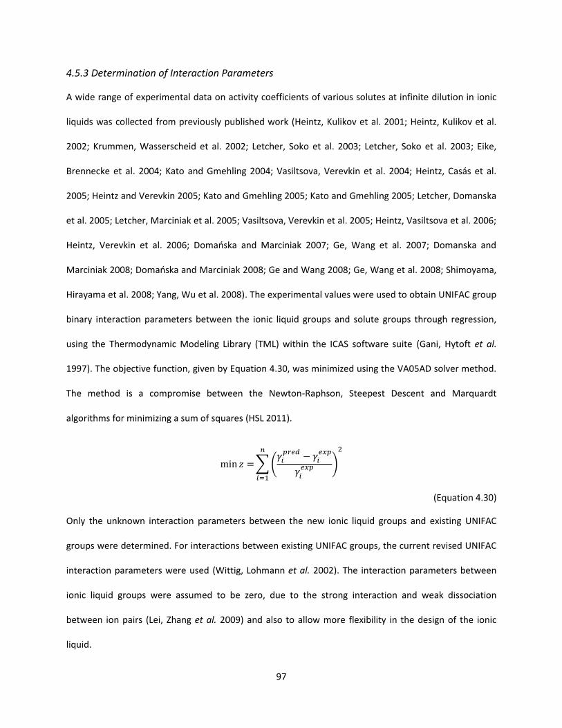
97
4.5.3 Determination of Interaction Parameters
A wide range of experimental data on activity coefficients of various solutes at infinite dilution in ionic
liquids was collected from previously published work (Heintz, Kulikov et al. 2001; Heintz, Kulikov et al.
2002; Krummen, Wasserscheid et al. 2002; Letcher, Soko et al. 2003; Letcher, Soko et al. 2003; Eike,
Brennecke et al. 2004; Kato and Gmehling 2004; Vasiltsova, Verevkin et al. 2004; Heintz, Casás et al.
2005; Heintz and Verevkin 2005; Kato and Gmehling 2005; Kato and Gmehling 2005; Letcher, Domans a
et al. 005 etcher, Marcinia et al. 005 Vasiltsova, Verev in et al. 005 Heintz, Vasiltsova et al. 00
Heintz, Verev in et al. 00 Doma s a and Marcinia 007 Ge, ang et al. 007 Domans a and
Marcinia 00 Doma s a and Marcinia 00 Ge and Wang 2008; Ge, Wang et al. 2008; Shimoyama,
Hirayama et al. 2008; Yang, Wu et al. 2008). The experimental values were used to obtain UNIFAC group
binary interaction parameters between the ionic liquid groups and solute groups through regression,
using the Thermodynamic Modeling Library (TML) within the ICAS software suite (Gani, Hytoft et al.
1997). The objective function, given by Equation 4.30, was minimized using the VA05AD solver method.
The method is a compromise between the Newton-Raphson, Steepest Descent and Marquardt
algorithms for minimizing a sum of squares (HSL 2011).
∑(
)
(Equation 4.30)
Only the unknown interaction parameters between the new ionic liquid groups and existing UNIFAC
groups were determined. For interactions between existing UNIFAC groups, the current revised UNIFAC
interaction parameters were used (Wittig, Lohmann et al. 2002). The interaction parameters between
ionic liquid groups were assumed to be zero, due to the strong interaction and weak dissociation
between ion pairs (Lei, Zhang et al. 2009) and also to allow more flexibility in the design of the ionic
liquid.
98
5.0 MOLECULAR DESIGN METHODS: THE REVERSE PROBLEM
Two main approaches were taken to address the reverse problem of CAMD: deterministic and
stochastic. Deterministic design was applied to solution of ionic liquid entrainers and is detailed in
Section 5.1. Tabu search, a stochastic method, was utilized for the design of ionic liquid extractants and
carbohydrate glass-formers, as described in Section 5.2. Additionally, two stochastic methods (tabu
search and genetic algorithms) were developed, tuned and compared for the design of carbohydrate
excipients in lyophilized protein formulations. Development is detailed in Section 5.3, tuning is explained
in Section 5.4 and the methods of solution comparison are given in Section 5.5.
5.1 DETERMINISTIC DESIGN OF IONIC LIQUID ENTRAINERS
Given an azeotropic mixture of interest, a CAMD problem was formulated to design an ionic liquid
entrainer. The solubility parameter is used as the target property. First, the design stage in the CAMD
problem selects all ionic liquids that have solubility parameters in a range between the azeotrope
mixture's solubility parameter and the entrained component's solubility parameter. From the initial
design step, several ionic liquid candidates can be generated. Next, the candidates are screened based
on other desirable properties such as melting temperature, thermal decomposition temperature, and
toxicity. The candidates remaining are then screened using the UNIFAC-IL model to determine how
much IL is needed to break the desired azeotrope. The candidates requiring minimal ionic liquid
concentrations are then finally screened based on distillation column energy requirements as
determined by simulation (see Section 6.0).
For the examples provided in this work, the property models for the screening of secondary properties
are not yet available. To provide an illustrative example of the proposed methodology, the initial
number of design candidates was limited. Only two candidates for each azeotropic mixture were
selected based on the extremes of the range of solubility parameters that are considered. One ionic
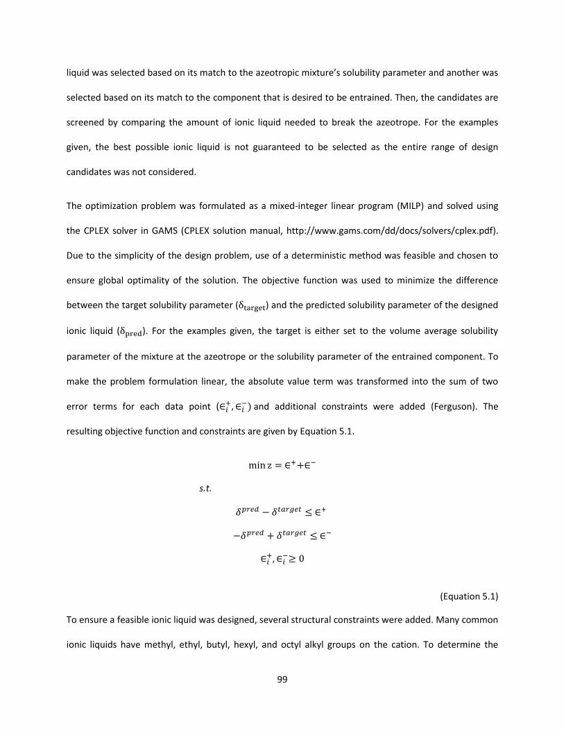
99
liquid was selected based on its match to the azeotropic mixture’s solubility parameter and another was
selected based on its match to the component that is desired to be entrained. Then, the candidates are
screened by comparing the amount of ionic liquid needed to break the azeotrope. For the examples
given, the best possible ionic liquid is not guaranteed to be selected as the entire range of design
candidates was not considered.
The optimization problem was formulated as a mixed-integer linear program (MILP) and solved using
the CPLEX solver in GAMS (CPLEX solution manual, http://www.gams.com/dd/docs/solvers/cplex.pdf).
Due to the simplicity of the design problem, use of a deterministic method was feasible and chosen to
ensure global optimality of the solution. The objective function was used to minimize the difference
between the target solubility parameter ( ) and the predicted solubility parameter of the designed
ionic liquid ( ). For the examples given, the target is either set to the volume average solubility
parameter of the mixture at the azeotrope or the solubility parameter of the entrained component. To
make the problem formulation linear, the absolute value term was transformed into the sum of two
error terms for each data point (
) and additional constraints were added (Ferguson). The
resulting objective function and constraints are given by Equation 5.1.
s.t.
(Equation 5.1)
To ensure a feasible ionic liquid was designed, several structural constraints were added. Many common
ionic liquids have methyl, ethyl, butyl, hexyl, and octyl alkyl groups on the cation. To determine the
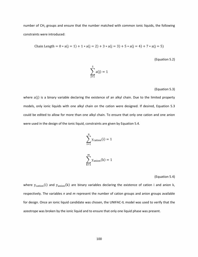
100
number of CH2 groups and ensure that the number matched with common ionic liquids, the following
constraints were introduced:
( ) ( ) ( ) ( ) ( )
(Equation 5.2)
∑ ( )
(Equation 5.3)
where ( ) is a binary variable declaring the existence of an alkyl chain. Due to the limited property
models, only ionic liquids with one alkyl chain on the cation were designed. If desired, Equation 5.3
could be edited to allow for more than one alkyl chain. To ensure that only one cation and one anion
were used in the design of the ionic liquid, constraints are given by Equation 5.4.
∑ ( )
∑ ( )
(Equation 5.4)
where ( ) and ( ) are binary variables declaring the existence of cation i and anion k,
respectively. The variables n and m represent the number of cation groups and anion groups available
for design. Once an ionic liquid candidate was chosen, the UNIFAC-IL model was used to verify that the
azeotrope was broken by the ionic liquid and to ensure that only one liquid phase was present.

101
5.2 USE OF TABU SEARCH IN DESIGN OF IONIC LIQUID EXTRACTANTS AND CARBOHYDRATE GLASS-
FORMERS
An existing molecular design framework was utilized for the design of ionic liquid extractants and
carbohydrate glass-formers (Eslick 2009; Eslick, Ye et al. 2009; McLeese, Eslick et al. 2010). Tabu search
was used to provide locally optimal solutions. The design targets for the two design problems are given
in Table 5.1.
Table 5.1 Property targets for molecular design using tabu search The tabu search was performed via a
modified version of Polymer Designer Pro (Eslick, Ye et al. 2009).
Ionic Liquid Extractant
Property Target
Partition coefficient (Kx) 50
Toxicity (lnEC50) 4.0
Carbohydrate Glass-Former
Property Target
Glass Transition Temperature of the Anhydrous Solute (Tg) 100°C
Glass Transition Temperature of the Maximally Freeze-Concentrated Solute (Tg’) -30°C
Melting Temperature of Ice (Tm’) -25°C
Concentration of the Maximally Freeze-Concentrated Solute (Cg’) 0.85
The existing molecular design framework was contained in a software package named Polymer Designer
(PD), written in C++ (Eslick 2009). For each design case, groups were changed to represent groups that
existed in the data set used to develop the corresponding property models. Design was limited to the
cation for the ionic liquid extactant case, with the anion set at tris(perfluoroalkyl)trifluorophosphate
(FAP). The groups used for both design problems are catalogued in Appendix C, along with general
102
guidelines for the use of PD. Additionally, the necessary property models were added to the program.
The tabu Search algorithm used in PD follows a procedure similar to the tabu Search algorithm
described in Section 5.3.3.
While useful for optimal structure determination, several factors necessitated the development of a
separate software package for design of carbohydrate excipients for lyophilized protein formulations.
The primary reason was the desire for comparison between tabu Search and genetic algorithms for use
in CAMD. A molecular representation that would be useful for both stochastic methods was necessary
for fair comparison. PD was developed with concern for cross-linked polymer systems and thus some
elements of the code were unnecessary for the design problems considered and added time to solution.
Additionally, tuning required easily editable parameter values. Any editing done to the source code or
group database for PD requires the program to be deleted and the code to be recompiled. The steps
needed for editing and recompiling the PD code are detailed in Appendix C. As the solution methods
needed to be ran many times for tuning purposes with different parameter values, ultimately the
existing framework proved too cumbersome. Development of a framework more suited to the desired
tasks is given in the following section.
5.3 DEVELOPMENT OF STOCHASTIC DESIGN METHODS FOR CARBOHYDRATE EXCIPIENTS IN
LYOPHILIZED PROTEIN FORMULATIONS
A CAMD framework for the design of carbohydrate excipients was developed for use with either tabu
search or a genetic algorithm. The framework was implemented in Visual Basic for Applications (VBA),
with Microsoft Excel used as the database for groups used in design. The overall framework is
diagramed in Figure 5.1.
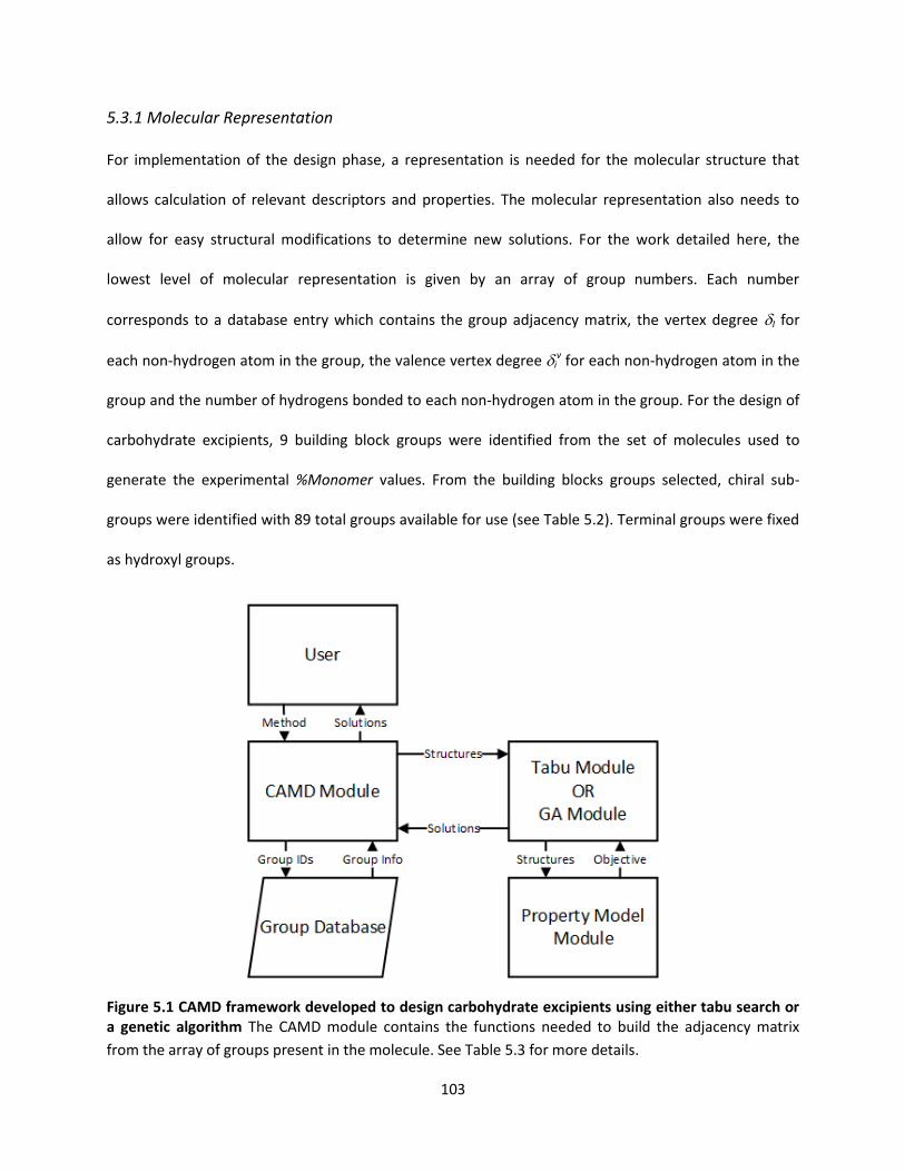
103
5.3.1 Molecular Representation
For implementation of the design phase, a representation is needed for the molecular structure that
allows calculation of relevant descriptors and properties. The molecular representation also needs to
allow for easy structural modifications to determine new solutions. For the work detailed here, the
lowest level of molecular representation is given by an array of group numbers. Each number
corresponds to a database entry which contains the group adjacency matrix, the vertex degree I for
each non-hydrogen atom in the group, the valence vertex degree iv for each non-hydrogen atom in the
group and the number of hydrogens bonded to each non-hydrogen atom in the group. For the design of
carbohydrate excipients, 9 building block groups were identified from the set of molecules used to
generate the experimental %Monomer values. From the building blocks groups selected, chiral sub-
groups were identified with 89 total groups available for use (see Table 5.2). Terminal groups were fixed
as hydroxyl groups.
Figure 5.1 CAMD framework developed to design carbohydrate excipients using either tabu search or a genetic algorithm The CAMD module contains the functions needed to build the adjacency matrix
from the array of groups present in the molecule. See Table 5.3 for more details.
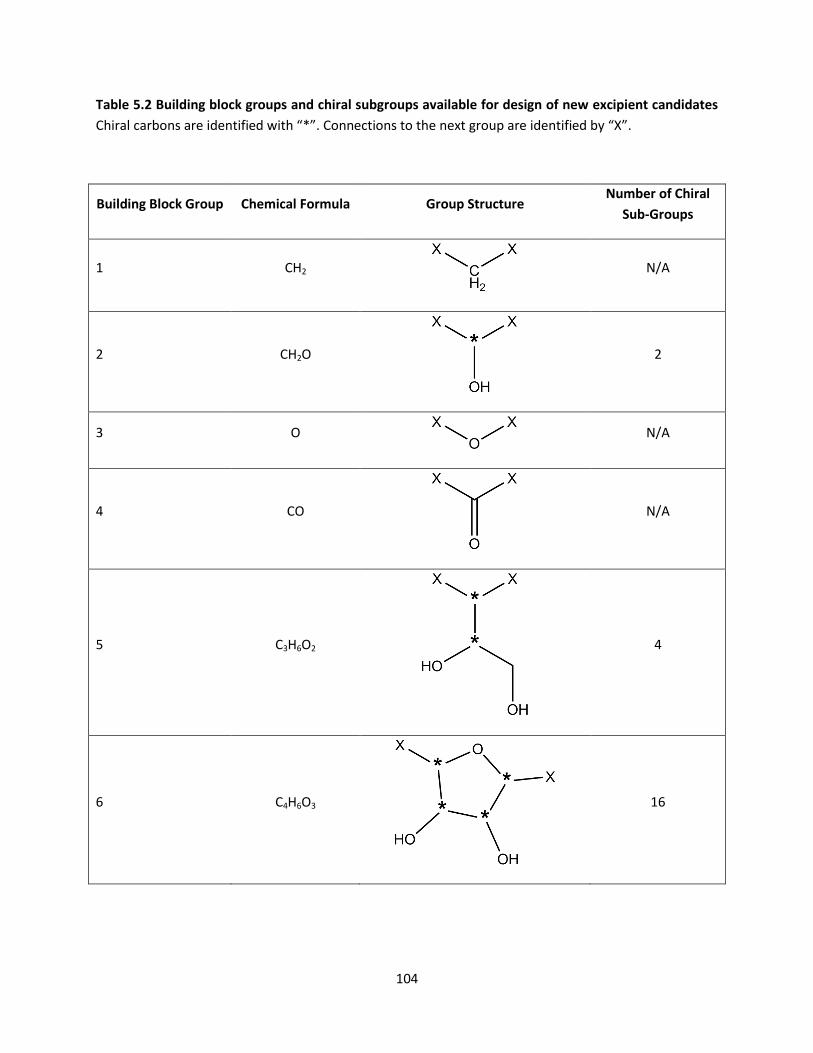
104
Table 5.2 Building block groups and chiral subgroups available for design of new excipient candidates
Chiral carbons are identified with “*”. Connections to the next group are identified by “X”.
Building Block Group Chemical Formula Group Structure Number of Chiral
Sub-Groups
1 CH2
N/A
2 CH2O
2
3 O
N/A
4 CO
N/A
5 C3H6O2
4
6 C4H6O3
16

105
7 C5H8O4
16
8 C5H8O3
16
9 C5H8O4
32
By factoring in chirality, there is an order of magnitude increase in the number of groups available for
selection during the generation of new candidate structures. The increase in the number of groups
available for selection has a marked impact on the number of possible molecular structure
combinations, resulting in a combinatorial problem. Figure 5.2 demonstrates how the number of
possible combinations increases exponentially as the number of groups available for selection increases.
For the design problem considered, the maximum number of groups selected is set at six as all
molecules used in the data set can be described by six or fewer of the groups given in Table 5.2. With a
maximum molecule size of six groups and 89 groups available for selection, 8.66x10⁸ combinations and
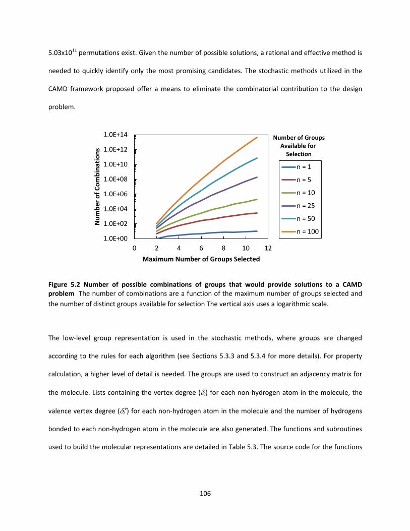
106
5.03x10¹¹ permutations exist. Given the number of possible solutions, a rational and effective method is
needed to quickly identify only the most promising candidates. The stochastic methods utilized in the
CAMD framework proposed offer a means to eliminate the combinatorial contribution to the design
problem.
Figure 5.2 Number of possible combinations of groups that would provide solutions to a CAMD problem The number of combinations are a function of the maximum number of groups selected and
the number of distinct groups available for selection The vertical axis uses a logarithmic scale.
The low-level group representation is used in the stochastic methods, where groups are changed
according to the rules for each algorithm (see Sections 5.3.3 and 5.3.4 for more details). For property
calculation, a higher level of detail is needed. The groups are used to construct an adjacency matrix for
the molecule. Lists containing the vertex degree (I) for each non-hydrogen atom in the molecule, the
valence vertex degree (iv) for each non-hydrogen atom in the molecule and the number of hydrogens
bonded to each non-hydrogen atom in the molecule are also generated. The functions and subroutines
used to build the molecular representations are detailed in Table 5.3. The source code for the functions
1.0E+00
1.0E+02
1.0E+04
1.0E+06
1.0E+08
1.0E+10
1.0E+12
1.0E+14
0 2 4 6 8 10 12
Nu
mb
er o
f C
om
bin
atio
ns
Maximum Number of Groups Selected
n = 1
n = 5
n = 10
n = 25
n = 50
n = 100
Number of Groups Available for
Selection

107
and subroutines is given in Appendix D. From the adjacency matrix and the lists, connectivity indices can
be calculated.

108
Table 5.3 Description of VBA functions and subroutines used for molecular representation Source code
can be found in Appendix D.
Function Name Argument(s) Resulting Value
atoms Number of group Number of atoms in group
name Number of group
String containing name of
worksheet in excel database
containing group structural
information
terminus
Number of group, number of atom in molecule
that represents the left-hand terminal atom in
group
Number of the atom in the
molecule that represents the
right-hand terminal atom in
group
Subroutine Name Argument(s) Result of Procedure
BuildMolecule
Array containing groups in molecule, array
containing the vertex degree (I) for each non-
hydrogen atom in the molecule, array containing
the valence vertex degree (iv) for each non-
hydrogen atom in the molecule, array containing
the number of hydrogens bonded to each non-
hydrogen atom in the molecule, array containing
adjacency matrix
Adds hydroxyl terminals to
both the first and last group
in the molecule. Updates
adjacency matrix and lists of
other structural values for
molecule represented by the
array containing the groups in
the molecule
GetConnectivity
Array containing the vertex degree (I) for each
non-hydrogen atom in the molecule, array
containing the valence vertex degree (iv) for
each non-hydrogen atom in the molecule, array
containing the number of hydrogens bonded to
each non-hydrogen atom in the molecule, array
containing adjacency matrix, number of non-
hydrogen atoms in the molecule, array
containing simple connectivity indices (),array
containing valence connectivity indices (v),
array containing average simple connectivity
indices (),array containing average valence
connectivity indices (v)
Updates chiral connectivity
index values for molecule
represented by the adjacency
matrix and lists of other
structural values
109
5.3.2 Calculation of Chiral Connectivity Indices and Objective Function
A depth-first search algorithm is used to determine the existence of paths in the adjacency matrix
ranging from lengths of zero to five (West 2001). The path length information is then used calculate the
chiral connectivity indices. Both the path search and connectivity index calculation are performed in the
GetConnectivity subroutine (see Table 5.3 and Appendix D). The calculated chiral connectivity indices
are used for property prediction, which is in turn used to calculate the objective function value. The
objective function is a characteristic CAMD type which describes the sum of the normalized absolute
differences between target properties and predicted properties (See Section 2.12 and Equation 2.8).
The objective function used has been modified by the inclusion of a penalty score and is given by
Equation 5.5. The penalty score is used to disallow final solutions from containing certain group
combinations that are unfavorable. In particular, the formation of peroxide bonds (O-O) and bonding of
two ring groups together are prevented through use of the penalty scores. Peroxides are undesired as
the bond is unstable. A bond between two rings in not wanted as such a bond is not observed in
carbohydrates. The penalty score is large enough to make objective function values for solutions
containing such structural features to be much larger in comparison to solutions without said features.
The penalty function along with the rules for adding and removing groups in each of the stochastic
design methods (explained further in Sections 5.3.3 and 5.3.4) eliminates the need for explicit structural
constraints. Additionally, the definition of groups eliminates the need to store the presence of double or
triple bonds in the adjacency matrix.
110
(∑
|
|)
s.t.
{
( )
( )
(Equation 5.5)
5.3.3 Tabu Search Algorithm
The tabu search algorithm utilizes solution history to generate locally optimal solutions to the molecular
design problem. In the following implementation, solutions are given as arrays of groups representing
the molecular structure. The tabu search algorithm developed is given in Figure 5.3. The tabu search
begins with a random initial solution which is generated by calling the InitialSolution subroutine (see
Table 5.4 and Appendix D). The connectivity indices are calculated for the initial solution and used to
determine the objective function. The solution is set as the current solution and then stored as the initial
entry in the tabu list. The information stored in the tabu list is comprised of the array of groups
comprising the molecule and the 0 value for checking to see if a solution is tabu.
The first iteration then begins by determining the number of neighbors to the current solution. The
number chosen is a random integer with a value between one and the set maximum number of
members to evaluate. A neighboring structure is generated through use of the Make_Neighbor function,
which takes the current solution’s array of groups as an argument and returns a neighboring solution’s
array of groups (see Appendix D). The Make_Neighbor function randomly selects one of four types of
local moves to be made to generate the neighboring solution. The types of moves are explained with
examples in Table 5.4.
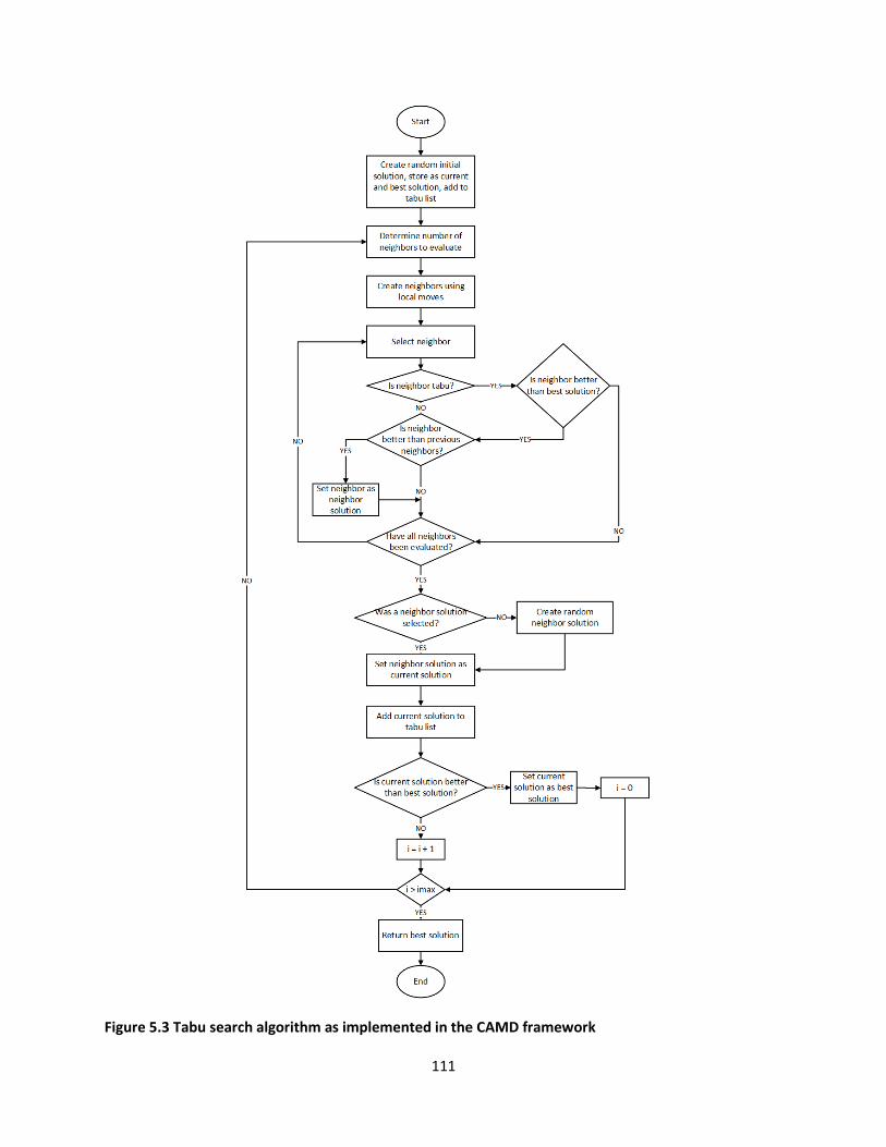
111
Figure 5.3 Tabu search algorithm as implemented in the CAMD framework
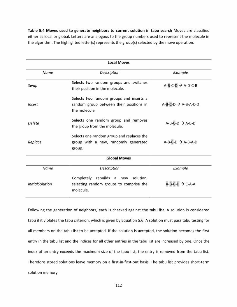
112
Table 5.4 Moves used to generate neighbors to current solution in tabu search Moves are classified
either as local or global. Letters are analogous to the group numbers used to represent the molecule in
the algorithm. The highlighted letter(s) represents the group(s) selected by the move operation.
Local Moves
Name Description Example
Swap Selects two random groups and switches
their position in the molecule. A-B-C-D A-D-C-B
Insert
Selects two random groups and inserts a
random group between their positions in
the molecule.
A-B-C-D A-B-A-C-D
Delete Selects one random group and removes
the group from the molecule. A-B-C-D A-B-D
Replace
Selects one random group and replaces the
group with a new, randomly generated
group.
A-B-C-D A-B-A-D
Global Moves
Name Description Example
InitialSolution
Completely rebuilds a new solution,
selecting random groups to comprise the
molecule.
A-B-C-D C-A-A
Following the generation of neighbors, each is checked against the tabu list. A solution is considered
tabu if it violates the tabu criterion, which is given by Equation 5.6. A solution must pass tabu testing for
all members on the tabu list to be accepted. If the solution is accepted, the solution becomes the first
entry in the tabu list and the indices for all other entries in the tabu list are increased by one. Once the
index of an entry exceeds the maximum size of the tabu list, the entry is removed from the tabu list.
Therefore stored solutions leave memory on a first-in-first-out basis. The tabu list provides short-term
solution memory.
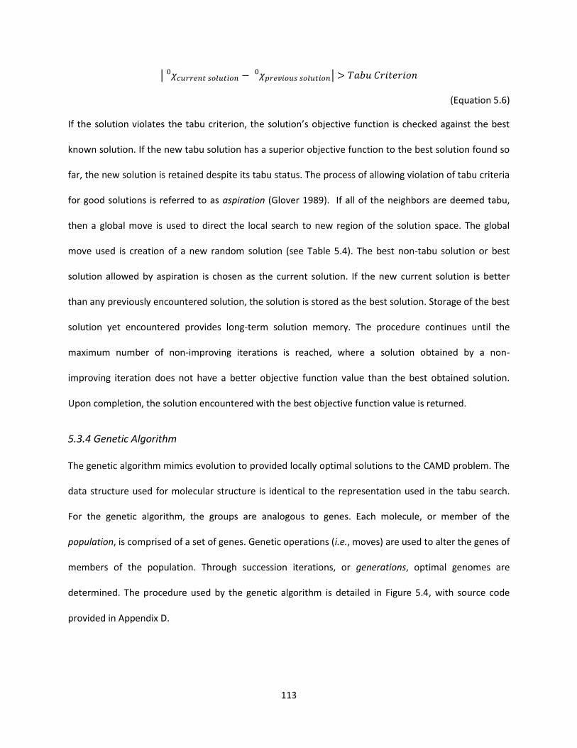
113
|
|
(Equation 5.6)
If the solution violates the tabu criterion, the solution’s objective function is chec ed against the best
known solution. If the new tabu solution has a superior objective function to the best solution found so
far, the new solution is retained despite its tabu status. The process of allowing violation of tabu criteria
for good solutions is referred to as aspiration (Glover 1989). If all of the neighbors are deemed tabu,
then a global move is used to direct the local search to new region of the solution space. The global
move used is creation of a new random solution (see Table 5.4). The best non-tabu solution or best
solution allowed by aspiration is chosen as the current solution. If the new current solution is better
than any previously encountered solution, the solution is stored as the best solution. Storage of the best
solution yet encountered provides long-term solution memory. The procedure continues until the
maximum number of non-improving iterations is reached, where a solution obtained by a non-
improving iteration does not have a better objective function value than the best obtained solution.
Upon completion, the solution encountered with the best objective function value is returned.
5.3.4 Genetic Algorithm
The genetic algorithm mimics evolution to provided locally optimal solutions to the CAMD problem. The
data structure used for molecular structure is identical to the representation used in the tabu search.
For the genetic algorithm, the groups are analogous to genes. Each molecule, or member of the
population, is comprised of a set of genes. Genetic operations (i.e., moves) are used to alter the genes of
members of the population. Through succession iterations, or generations, optimal genomes are
determined. The procedure used by the genetic algorithm is detailed in Figure 5.4, with source code
provided in Appendix D.

114
The search for solutions begins with random generation of members of the population through use of
the InitialSolution subroutine (see Table 5.4 and Appendix D). The size of the population determines the
number of solutions that are evaluated and generated during each generation. The fitness is determined
for each member of the population, where the fitness is given as the inverse of the objective function
(e.g., when the objective function is minimized, the fitness is maximized). The fitness is used to
calculate the probability (as a %) that a member will become a parent for the next generation through
use of Equation 5.7. A parent is a member which undergoes a move to create a new member.
( ) ( ( )
∑ ( )
)
(Equation 5.7)
Where Fit(j) represents the fitness of the j-th member of the population of size n. Once the probability is
determined for a member, a roulette selection is used to determine whether the member will be a
parent. A random integer between zero and the maximum allowable probability is chosen. If the integer
is less than the probability calculated for the member, the member is chosen as a parent. Due to the
semi-random selection, any number of members may become parents but members with higher fitness
values are more likely to become parents. If no parents are chosen, then two parents are randomly
selected from the population. The fitness of the selected parents is checked against the fitness of the
best encountered solution. If the fitness exceeds the best known, the parent is retained in the next
generation through a rule known as elitist policy (Venkatasubramanian, Chan et al. 1995).

115
Figure 5.4 Genetic algorithm as implemented in the CAMD framework

116
Table 5.5 Moves used to generate offspring to selected parents in the genetic algorithm Moves require
either one parent or two parents. Letters are analogous to the genes or group numbers used to
represent the molecule in the algorithm. The highlighted letter(s) represents the gene(s) selected by the
move operation. Bold font is used in the two parent moves to distinguish groups belonging to the
second parent.
One Parent Moves
Name Description Example
Hop Selects two random genes and switches their
position in the molecule. A-B-C-D A-D-C-B
Insert Selects two random genes and inserts a random
gene between their positions in the molecule. A-B-C-D A-B-A-C-D
Delete Selects one random gene and removes the gene
from the molecule. A-B-C-D A-B-D
Mutate Selects one random gene and replaces the gene
with a new, randomly generated gene. A-B-C-D A-B-A-D
Two Parent Moves
Name Description Example
Blend Combines two parent molecules end to end to
create one offspring molecule. A-B + C-D A-B-C-D
Crossover
Selects a random gene in each parent molecule
to use as a crossover point, generating two
offspring molecules.
A-B-C-D + A-B-C-D
A-C-D + A-B-B-C-D
New members for the next generation are produced by randomly selecting two parents from the list of
parents generated through the roulette selection. The parents’ structures (given as group arrays) are
used as arguments in the Make_Offspring function (see Appendix D). The Make_Offspring randomly
selects either a one parent move or a two parent move to generate a new member for the next
generation (see Table 5.5). Each move is analogous to known genetic operations that occur in genomes
of organisms. Comparison shows that all one parent moves have matching local moves in the tabu

117
search algorithm (see Table 5.4). Following the generation of all new members of the population, the
next generation begins. The genetic algorithm proceeds for a set number of maximum generations,
returning the member with the highest fitness from the last generation.
5.4 TUNING OF STOCHASTIC DESIGN METHODS FOR CARBOHYDRATE EXCIPIENTS IN LYOPHILIZED
PROTEIN FORMULATIONS
The objective of tuning is to produce a stochastic design method that efficiently produces high quality
solutions. Efficiency is measured by the time to solution and quality is measured by the solution’s
objective function value. Each design method contains several key parameters whose values affect the
solution search. Tuning provided the rationale behind the values used for the parameter values in each
design method. During tuning, a parameter was changed while all other values were kept constant. For
each adjusted parameter value, 100 runs were performed with the objective values and times to
solution captured for each run. The process was repeated for each parameter of interest.
From the observations, parameter values were chosen to yield a high percentage of high quality
solutions (designed molecules with property values within 5% of the target property values) while
minimizing the time to solution. The parameters tuned for each method are detailed in the following
subsections. The parameters are not exhaustive for the two stochastic methods considered, but do
represent the key parameters for the methods as developed here. Different implementations of tabu
search and genetic algorithms may use slightly different parameters to guide the search for new
solutions than the parameters presented here. The parameters used here were chosen to allow the best
comparison possible between the two methods for CAMD applications.
A simple test case with a known global optimum was used as the test case for tuning. Each algorithm
was used to generate solutions with a target molecular weight of 342 g/mol. For tuning, penalty

118
functions were not employed in the objective function. The only other difference between the tuning
and final design runs is the property model that is used, which does not affect the search process and
only affects the objective function calculated for a given molecular structure. Thus it is expected that the
tuning results would hold for any other CAMD design case where only the property model is altered.
5.4.1 Tabu Search Algorithm
For the tabu search algorithm, four parameters were used for tuning:
Maximum number of non-improving iterations – determines how long the search will be
performed.
Maximum number of neighbors evaluated per iteration – determines how many new solutions
to consider at each iteration.
Size of tabu list – determines how many previous solutions are stored in memory. Also effects
the time spent checking to see if a solution is tabu.
Tabu criterion – determines how likely a solution is to be considered tabu.
The base parameter values are presented in Table 5.6.
Table 5.6 Parameter values used for the base case during tuning of the tabu search Parameters were
altered on at a time to observe the effects of the parameter value on solution quality and time to
solution.
Parameter Base Value
Maximum number of non-improving iterations 10
Maximum number of neighbors evaluated per iteration 2
Size of tabu list 10
Tabu criterion 0.5
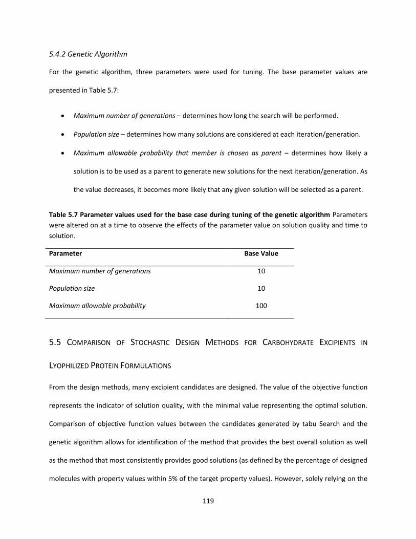
119
5.4.2 Genetic Algorithm
For the genetic algorithm, three parameters were used for tuning. The base parameter values are
presented in Table 5.7:
Maximum number of generations – determines how long the search will be performed.
Population size – determines how many solutions are considered at each iteration/generation.
Maximum allowable probability that member is chosen as parent – determines how likely a
solution is to be used as a parent to generate new solutions for the next iteration/generation. As
the value decreases, it becomes more likely that any given solution will be selected as a parent.
Table 5.7 Parameter values used for the base case during tuning of the genetic algorithm Parameters
were altered on at a time to observe the effects of the parameter value on solution quality and time to
solution.
Parameter Base Value
Maximum number of generations 10
Population size 10
Maximum allowable probability 100
5.5 COMPARISON OF STOCHASTIC DESIGN METHODS FOR CARBOHYDRATE EXCIPIENTS IN
LYOPHILIZED PROTEIN FORMULATIONS
From the design methods, many excipient candidates are designed. The value of the objective function
represents the indicator of solution quality, with the minimal value representing the optimal solution.
Comparison of objective function values between the candidates generated by tabu Search and the
genetic algorithm allows for identification of the method that provides the best overall solution as well
as the method that most consistently provides good solutions (as defined by the percentage of designed
molecules with property values within 5% of the target property values). However, solely relying on the

120
objective function value may be misleading as many candidates could have statistically similar property
values to best solution and thus be solutions of equal quality.
A QSPR’s use lies in predicting a property for a new molecule of interest, represented by the molecular
descriptors. The resulting predicted value has some error term involved. A novel approach to design
solution comparison using prediction intervals was utilized. Prediction intervals allow for the error from
the fitted model as well as any error in a future observation to be quantified (Wasserman 2004). A
confidence interval only accounts for error in the correlation, so a prediction interval is always larger
than a confidence interval. A 1 - prediction interval for a predicted property of interest is given by
Equation 5.8.
⁄ √ ( ( ) )
Equation 5.8
where ⁄ is the student’s t-test value for the given degrees of freedom, is the vector of descriptors
used in the prediction, is the transposed vector of descriptors used in the prediction, is the matrix
of descriptors used to build the correlation, is the transposed matrix of descriptors used to build the
correlation, and is the unbiased estimator of the model variance.
Given the connectivity indices for a designed carbohydrate excipient, new property values were
predicted. Using the connectivity index values, R was used to calculate prediction intervals at a 95% level
(The R Project for Statistical Computing, www.r-project.org). The procedure used in R for calculation of
prediction intervals along with sample code is given in Appendix B. The prediction intervals were
included to provide a reasonable range for the expected properties of the designed excipient molecule.
The prediction intervals were also used to determine if two solutions from the optimal design phase
were statistically different once the solutions were found using either tabu search or a genetic
algorithm. When comparing the predicted properties of two designed molecules, overlapping prediction

121
intervals indicate that the solutions are not statistically different. The use of prediction intervals to
compare solutions represents a novel approach to evaluating solutions generated in computer-aided
molecular design.
122
6.0 SIMULTANEOUS PRODUCT AND PROCESS DESIGN
CAMD was linked with separation process design for the simultaneous design of an ionic liquid entrainer
and azeotropic separation process. Key to the IL-based separation process is the extractive distillation
column, where the azeotrope is broken. Once a candidate was designed and confirmed to break an
azeotrope of interest using the UNIFAC-IL model, design of the separation process was performed. The
extractive distillation column was designed using the driving force method, as detailed in Section 6.1.
After design of the column, simulations were used to design the ionic liquid recovery unit and to
determine overall heat duty for the process. The simulation procedure is given in Section 6.2. The overall
feedback between product and process design is outlined in Figure 6.1. Details concerning the molecular
design component can be found in Section 5.1.
Figure 6.1 Overall methodology for simultaneous design of ionic liquid entrainers and IL-based separation processes Figure is adapted from (Roughton, Christian et al. 2012).
Yes
Simulate
process
Finalize design
Adjust
process
design
No, select
next best
Optimally design or select from database
Choose Azeotrope for Separation
Set solubility parameter
target and other property
constraints
Is azeotrope
broken?
Generate driving force
diagram and design
separation process
Evaluate
results
Final IL-based separation
process chosen
Adjust target properties

123
6.1 DRIVING FORCE BASED DESIGN
For separation of a given azeotrope, an extractive distillation column was designed using the driving
force method. The driving force is defined as the difference between the vapor and liquid composition
of the light key component (Bek-Pedersen, Gani et al. 2000). The driving force is used to evaluate the
feasibility of a proposed separation process, ensuring that the driving force is never zero (Bek-Pedersen,
Gani et al. 2000). By designing the separation process based upon the maximum driving force, near
optimal distillation columns can be designed with respect to energy requirements (Gani and Bek-
Pedersen 2000).
The UNIFAC-IL model was used to generate the driving force for each ternary system consisting of the
binary azeotrope plus an ionic liquid. The two components comprising the azeotropic mixture were
defined as the key binary mixture. Product purities of the azeotrope components (on an ionic liquid free
basis) were specified at ASTM purity standards. The driving force was plotted against the light key
component mole fraction and the location (Dx) and value (Dy) of the maximum driving force was
determined for varying ionic liquid compositions. The number of stages (N) were determined by finding
the minimum number of stages necessary to achieve the desired product specifications, as determined
by rigorous simulation (detailed in section 2.3.2). As the location of the maximum driving force was
determined on an ionic liquid free basis, the location was modified using Equation 6.1. The driving force
profile is only an estimate for the systems considered, as the ionic liquid concentration may vary
throughout the column. The feed stage location (NF) was determined using Equation 6.2 (Gani and Bek-
Pedersen 2000) with a modification due to one stage being used as the entrainer feed stage.
( )
(Equation 6.1)

124
( )( )
(Equation 6.2)
The original driving force method was proposed for systems with one feed. The proposed distillation
column consists of a main feed for the azeotropic mixture and an ionic liquid feed at the top of the
tower. For moderate to high ionic liquid concentrations, scaling of the feed tray location may be
necessary. The scaling factor (SF) is given by Equation 6.3, where is the specification for the light
key distillate mole fraction and is the specification for the heavy key bottoms mole fraction (Bek-
Pedersen, Gani et al. 2000). Calculation of and is performed taking into account the ionic
liquid present in the column. When SF ≤ 0.01 and < 0.7, scaling is necessary and Equation 6.4 is used
to determine the site where the feed stage should be relocated in the column. In the initial
implementation of driving force based design, the feed stage will always move up the column between a
minimum of 10% of the total number of trays when scaling is required. By scaling the feed tray location
through use of Equation 6.4, a more accurate location is determined then by relocating either by 5% or
10% as proposed by Bek-Pedersen et al. (Bek-Pedersen, Gani et al. 2000). By using the scaled feed tray
location when the stated conditions are met, a near-optimal column design is achieved with respect to
overall energy consumption for a column with a main feed and a separate ionic liquid feed.
(Equation 6.3)
[ ( )]
(Equation 6.4)
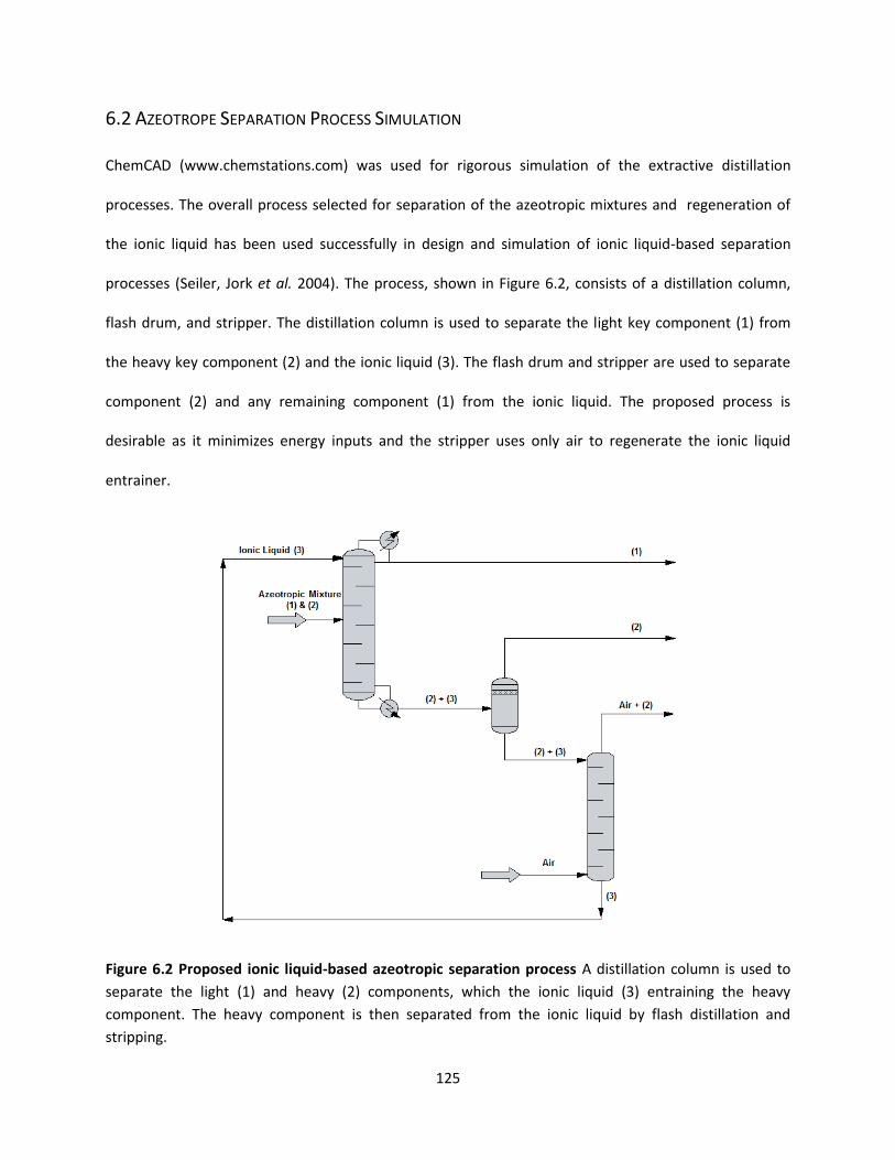
125
6.2 AZEOTROPE SEPARATION PROCESS SIMULATION
ChemCAD (www.chemstations.com) was used for rigorous simulation of the extractive distillation
processes. The overall process selected for separation of the azeotropic mixtures and regeneration of
the ionic liquid has been used successfully in design and simulation of ionic liquid-based separation
processes (Seiler, Jork et al. 2004). The process, shown in Figure 6.2, consists of a distillation column,
flash drum, and stripper. The distillation column is used to separate the light key component (1) from
the heavy key component (2) and the ionic liquid (3). The flash drum and stripper are used to separate
component (2) and any remaining component (1) from the ionic liquid. The proposed process is
desirable as it minimizes energy inputs and the stripper uses only air to regenerate the ionic liquid
entrainer.
Figure 6.2 Proposed ionic liquid-based azeotropic separation process A distillation column is used to
separate the light (1) and heavy (2) components, which the ionic liquid (3) entraining the heavy
component. The heavy component is then separated from the ionic liquid by flash distillation and
stripping.

126
Fixed parameters for the process were chosen to match previous simulation work (Seiler et al., 2004) for
comparison of results. For both the acetone-methanol and ethanol-water azeotropes, a total feed rate
of 200 kmol per hour was used. Ionic liquid feed rate, column size, and feed tray location were altered
to minimize energy consumption of the column. The distillate specifications were set to ASTM standards
for purity. The azeotropic mixture was fed as a saturated liquid. The ionic liquid was fed at the same
temperature as the feed. First approximation of the feed stage location was obtained using the driving
force method as outlined in the previous section. The location was then moved above and below the
initial stage to ensure that energy use was minimized. The procedure was repeated for varying flow
rates of ionic liquid until a column configuration and entrainer flow rate that minimized overall energy
consumption was identified. The values of the free variables for the entire distillation and entrainer
regeneration process were determined by the ChemCAD solver such that overall energy requirements
were minimized, while also satisfying constraints on column size, air flow rate and final product purity of
the ionic liquid entrainer leaving the column (specified as 99.9% pure on a molar basis). The fixed
parameters and free process variables are outlined in Table 6.1 for both azeotropic systems.
Prediction of heat capacity was needed for the ionic liquids in order to accurately calculate the energy
requirements of the proposed separation processes. Group contribution models from literature were
used to predict the isobaric heat capacities of the ionic liquids used in the simulations (Gardas and
Coutinho 2008; Ren, Zhao et al. 2011). Column simulation was performed for both the optimal and non-
optimal ionic liquid entrainers (selected for comparison purposes). The entire process, including
entrainer regeneration, was performed only for the best ionic liquid candidates. Energy requirements
for the ethanol-water separation were compared to results found for an ionic liquid known to
experimentally break the given azeotropes but not designed with CAMD methods (henceforth referred
to as an experimentally-selected ionic liquid) and also for a conventional entrainer (Seiler, Jork et al.
2004).

127
Table 6.1 Fixed parameters and free variables for ionic liquid-based extractive distillation processes
Fixed Parameters
Acetone-Methanol Ethanol -Water
Distillation Column
Operating pressure [atm] 1.00 1.00
Column Feed
Flow rate [kmol/hr] 200 200
x1 0.5 0.7
x2 0.5 0.3
Distillate
Flow rate [kmol/hr] 100 140
x1 0.995 0.998
Flash Tank
Operating pressure [atm] 0.10 0.10
Stripper
xIL (bottom) 0.999 0.999
Air temperature [K] 298.15 298.15
Free Variables
Distillation Column
Number of stages
Feed stage
Reflux ratio
Flash Tank
Temperature
Stripper
Number of stages
Air flow rate

128
7.0 MOLECULAR SIMULATION FOR DESIGN AND POST-DESIGN STAGES
Stabilizing additives, or excipients, are often included in lyophilized formulations to reduce aggregation.
Nonionic surfactants have been shown to bind with weak affinity to proteins (McNally and Hastedt
2008). Such binding could interact with hydrophobic regions on the protein and limit access to
aggregation prone “hot spots”. Nonionic surfactants such as Tween 80 have been shown to decrease
aggregation in lyophilized protein formulations (Kerwin 2008). However, difficulties can arrise during the
lyophilization process due to the low glass transition temperatures exhibited by surfactants (McNally
and Hastedt 2008). A successful formulation using surfactants requires the presence of glass formers,
such as sugars or polymers.
Sugar molecules have also been shown to exhibit site-specific effects on proteins during lyophilization
through use of hydrogen-deuterium exchange mass spectroscopy (Li, Williams et al. 2008), indicating
that interaction between sugars and proteins occur in the lyophilized state. Such interactions can be
exploited to provide better coverage of aggregation prone “hot spots” on the protein. By selecting
excipients that interact preferably with aggregation prone regions, a lyophilized formulation can be
developed to reduce aggregation.
In following section, a simulation-guided design approach is utilized to select a sugar and surfactant pair
that optimally provides the most interaction with an aggregation prone region on the protein
calmodulin (Protein ID #1CLL, Protein Data Bank via http://www.rcsb.org/pdb/home/home.do). By
choosing a formulation with maximal protein-excipient interactions, the potential for aggregation is
reduced. While surfactants may interact more than sugars on a per molecule basis, a sugar was included
to ensure that a stable glass could be formed. The use of molecular docking simulations to aid in post-
design screening is also proposed.

129
7.1 USE OF AUTODOCK FOR BLIND DOCKING SIMULATIONS Molecular simulation results were generated for use in guiding formulation design. The tool used for
molecular simulation was AutoDock (http://autodock.scripps.edu/), which utilizes blind docking to
determine regions of protein-ligand interaction with no a priori knowledge of binding site (Huey, Morris
et al. 2007). AutoDock employs a grid-based approach along with a semiempirical free energy force field
to identify interaction sites with minimal free energy (Huey, Morris et al. 2007). AutoDock leaves the
protein as a rigid molecule and only adjusts the ligand conformation. The ligand conformation is
described by rotation, translation and torsional degrees of freedom (Goodsell, Morris et al. 1996).
Search for conformations is guided by one of three stochastic optimization methods chosen by the user:
Monte Carlo simulated annealing, traditional genetic algorithm and Lamarkian genetic algorithm
(Morris, Goodsell et al. 1998). As all solution methods are stochastic, the conformations returned are
local optima. The work presented here employs the simulated annealing method. Blind docking has
proved successful in detecting binding sites on proteins for small molecule drug-like compounds
(Hetényi and van der Spoel 2006) and peptides (Hetényi and van der Spoel 2002), which encompass the
size of descriptors considered here.
7.2 DETERMINATION OF PROTEIN-EXCIPIENT INTERACTIONS To predict the amino acids of calmodulin most likely to interact with a given excipient, blind docking
simulations were performed using AutoDock. Each simulation provided ten docking conformations that
provided the lowest free energy of the conformations encountered. Five simulations were done for each
excipient with calmodulin, providing fifty docking conformations total for each excipient. Each
conformation was analyzed to determine which resides were in contact, through hydrogen bonding,
with the excipient molecule. An important limitation to note is that the blind docking simulations do not
consider that the protein is lyophilized but rather employ an implicit solvation model. It follows that the
approach used for estimating protein-excipient interactions does not take into account any dynamics

130
that may result from the lyophilization process. The approach only provides a first-approximation of
protein-excipeint interactions that may be present. Docking free energy calculations are therefore not
instructive to the approach taken and are not utilized.
The computational results from Autodock were qualitatively compared to experimental hydrogen-
deuterium exchange (HDX) mass spectroscopy experiments using lyophilized formulations of calmodulin
and either trehalose, sucrose, raffinose, or mannitol (Li, Williams et al. 2008). Regions of the protein that
are able to freely exchange hydrogen for deuterium are exposed and are not protected by protein-
excipient interactions. Experimentally, the extent of protein-excipient interactions is inversely related to
deuterium uptake. For comparison between experimental and simulation results, it is expected that
regions of high protein-excipient interaction identified by simulation should correspond with regions of
low deuterium uptake experimentally.
7.3 OPTIMAL SELECTION OF EXCIPIENTS Contact information provided by the docking simulations was used to optimally select excipients that
have the highest number of interactions with aggregation prone “hot spots”. The hot spots were
predicted using Aggrescan (Conchillo-Sole, de Groot et al. 2007). For each hot spot, a sugar and a
surfactant molecule were chosen to maximize protein-excipient interactions. For selection purposes,
whichever excipient had the most interactions with a particular residue was chosen as the best
candidate. It was assumed that the molecule with the most interactions with a residue would have the
dominant effect and thus contribute the most to the protection of the residue of interest. At each
residue in the hot spot, the best sugar candidate and the best surfactant candidate were compared.
Whichever excipient had the most interactions was selected and the process was repeated for the entire
hot spot sequence. The sugar-surfactant pair that provided the maximum number of interactions was
selected as the optimal drug formulation. The formulation of the optimization problem is given in

131
Equation 7.1. The problem is formulated as a MINLP and was solved using the DICOPT solver in GAMS
(GAMS documentation, http://www.gams.com/).
n
i
i scoren interactiomax
1,0,,,
1
1
1
scoresugar
score surfactant
score surfactant
scoresugar
score surfactant
scoresugar
score surfactantscoresugar scoren interactio
s.t.
tan
3
1
4
1
tan
tan
3
1
4
1
tan
kjtsurfacsugar
k
k
j
j
tsurfacsugar
tsurfac
sugar
k
kk
j
jj
tsurfacsugar
yyyy
y
y
iyiy
i
iiy
i
iiy
iscoreyi
iscoreyi
iiyiiyi
(Equation 7.1)
where i is a residue location, n is the number of residues in the hot spot of interest, j is a specific sugar,
and k is a specific surfactant. The scorej(i) and scorek(i) are input as parameters based on the results
from molecular docking. The scores are integer values, but are not explicitly defined as such in GAMS.
The constraints ensure that the highest interaction score between a sugar and a surfactant is chosen for
each residue. The constraints provide an interaction score that is summarized below, without the need
for disjunctive programming:
scoresugar score surfactant if score surfactant
score surfactant scoresugar if scoresugar )( scoren interactio
iii
iiii
(Equation 7.2)

132
7.4 DOCKING SIMULATION RESULTS Docking simulations providing fifty conformations were performed individually for mannitol, trehalose,
sucrose, raffinose, octyl glucoside, tween 40, and tween 80 with the protein calmodulin. The results for
the sugars were compared to experimental HDX results. Overall, the docking results compared favorably
with the HDX results. Regions of high interactions in the docking simulations corresponded to regions
that were protected from hydrogen/deuterium exchange. The histogram of interactions versus residue
location is provided in Figure 7.1 for trehalose. Residues that interacted frequently with trehalose match
well with the shaded regions indicating protection from hydrogen/deuterium exchange.
Figure 7.2 provides a visual comparison of the regions with high interaction and the regions protected
from exchange for the trehalose-calmodulin system. From the comparison of the computational and
experimental results, the docking simulations provide a reasonable prediction of the residues involved in
protein-excipient interactions and provide a useful tool for selecting excipients for lyophilized protein
formulations.

133
Figure 7.1 Frequency of amino acid residues of calmodulin in contact with trehalose Results are given
for 50 docking conformations. The shaded regions indicate amino acids that were protected by
trehalose in the lyophilized state, as determined by HDX experiments (Li, Williams et al. 2008). Figure
adapted from (Roughton, Pokphanh et al. 2012).
Figure 7.2 Trehalose interaction regions mapped to the surface of calmodulin Blue regions indicate
residues that interacted with trehalose in more than three conformations. Red regions indicate regions
that were protected by trehalose in the lyophilized state, as determined by HDX experiments. Purple
regions are theintersect of the computationally predicted high interaction regions and the
experimentally determined protected regions. Figure adapted from (Roughton, Pokphanh et al. 2012).
0
0.2
0.4
0.6
0.8
1
1.2
0
2
4
6
8
10
12Fr
eq
uen
cy o
f R
esid
ues
in C
on
tact
w
ith
Lig
and
(p
er 5
0 c
on
form
atio
ns)
Amino Acid Position
Frequency HD Exchange

134
7.5 FORMULATION SELECTION FOR MAXIMIZING PROTEIN-EXCIPIENT INTERACTIONS Using the docking simulation results and the previously described optimization problem formulation,
sugar-surfactant pairs were selected for each hot spot region on calmodulin. The hot spots were
predicted using Aggrescan (Conchillo-Sole, de Groot et al. 2007). Due to the proximity of hot spots 4 and
5, a formulation was also selected for the combined region. The results are given in Table 7.1. The
interaction scores provided correspond to the number of interactions exhibited in the docking
simulations.
Table 7.1 Sugar-surfactant formulations selected for maximum interaction with hot spot regions Table
adapted from (Roughton, Pokphanh et al. 2012).
Hot
Spot
Amino
Acids Sugar Surfactant
Combined
Interaction
Score
Sugar
Interaction
Score
Surfactant
Interaction
Score
1 15-19 Trehalose Tween 40 24 10 24
2 33-38 Mannitol Tween 40 13 10 7
3 67-73 Sucrose Tween 40 17 9 15
4 99-103 Raffinose Octyl Glucoside 10 7 8
5 106-111 Raffinose Tween 80 17 11 13
6 141-145 Raffinose Octyl Glucoside 26 15 26
4 & 5 99-111 Raffinose Octyl Glucoside 29 18 22
The results show that the excipients providing maximal interactions vary from hot spot to hot spot. All
available excipients were selected at least once. The addition of a sugar provided no additional
interactions for the formulations selected for hot spots 1 and 6 and thus was not beneficial from a
protein-excipient interaction standpoint. A sugar would be necessary to ensure a stable glass was
formed during the lyophilization.
The procedure outlined above could be used for any number of excipients and proteins to predict
formulations with maximal protein-excipient interactions. By maximizing protein-excipient interactions,
the aggregation propensity is reduced and a safer, more effective drug product is produced. The fact

135
that the sugar-surfactant pair providing maximal interactions differed between hotspots highlights the
complexity of selecting beneficial excipients for a lyophilized protein formulation.
While the proposed approach may have some application in the design phase of CAMD (as outlined
above), a potentially more useful application is for post-design review. Following design, promising
candidates could be further screened using a molecular docking approach to identify candidates with
benficial protein-excipient interactions. Molecular docking provides a faster screening procedure than
HDX experiments, which would be especially useful for large candidate lists. Following screening by
molecular docking, HDX experiments can provide final verification and selection of design candidates. It
is noted that additional protein-excipient systems have been explored using the molecular simulation
approach outlined by Anthony I. Pokphanh and Haider S. Tarar at the University of Kansas. The data they
have collected is not included in the presented work, but also provides good comparison to
corresponding experimental HDX studies.
136
8.0 RESULTS FOR IONIC LIQUID DESIGN
The following section contains the modeling and molecular design results for the two ionic liquid design
examples considered: sections 8.1-8.3 are concerned with entrainer design and sections 8.4-8.5 are
concerned with extractant design for in situ fermentation.
The group contribution model for ionic liquid solubility parameter is presented in Section 8.1. The
acetone-methanol and ethanol-water azeotropes were chosen for evaluation of the CAMD methodology
for design of ionic liquid entrainers. In addition, the 1-propanol-water, 2-propanol-water, and ethyl
acetate-ethanol azeotropes were used for evaluation of the UNIFAC-IL predictions in Section 8.2. The
molecular design results for the ionic liquid entrainer case are presented in Section 8.3 and the
separation process design results are given in Section 8.4.
The connectivity index models for both the partition coefficient of NDHD in ionic liquid and ionic liquid
toxicity are presented in Section 8.5. Design results for ionic liquid extractant design obtained through
tabu search are discussed in Section 8.6.
8.1 HILDEBRAND SOLUBILITY PARAMETER GROUP CONTRIBUTION MODEL
Experimental values for 24 different ionic liquids was used for the development of the Hildebrand
solubility parameter GC model (Marciniak 2010). In addition to 3 terms for the alkyl chain groups, 5
cation and 12 anion groups were used to describe the ionic liquids in the data set. The total number of
independent variables in the model are 21 (including a constant term), giving 3 degrees of freedom. The
degrees of freedom are relatively low, which is a consequence of the use of group contribution models
with small data sets. The developed model (see Equation 4.17) provides a good fit of experimental data
with a value of 0.34 %AARD between the predicted and experimental solubility parameter values. The
maximum relative deviation observed was 0.305. The results are shown in Figure 8.1.

137
Figure 8.1 Comparison between experimental and predicted solubility parameter values Predictions
were made using the group contribution model shown in Table 8.1. Experimental ionic liquid solubility
values are obtained from (Marciniak 2010). Figure adapted from (Roughton, Christian et al. 2012).
The contributions for each group are given in Table 8.1 Increasing the alkyl chain length decreases the
overall solubility parameter value, as the value for CH2 groups is negative. Ionic liquids with pyridinium
cations are usually more hydrophobic than those with imidazolium cations (Papaiconomou, Salminen et
al. 2007), reflected in the model by the smaller contribution for the pyridinium cation compared to the
imidazolium cation. In general, the many of the anion contributions are larger in magnitude than the
commonly encountered imidazolium, pyridinium, and pyrrolidonium cation contributions. For the design
examples, only imidazolium and pyridinium cations were used as cation choices to ensure that the
UNIFAC-IL model could be used to predict VLE. The minimum solubility parameter value predicted by
the model using the design problem’s cation restrictions was 17.8 MPa1/2 for 1-octyl-4-methylpyridinium
chloride. The maximum solubility parameter value predicted was 32.6 MPa1/2 for 1,3-
dimethylimidazolium tetrafluoroborate.
15
20
25
30
35
15 20 25 30 35
Pre
dic
ted
[
MP
a1/2 ]
Experimental [MPa1/2]
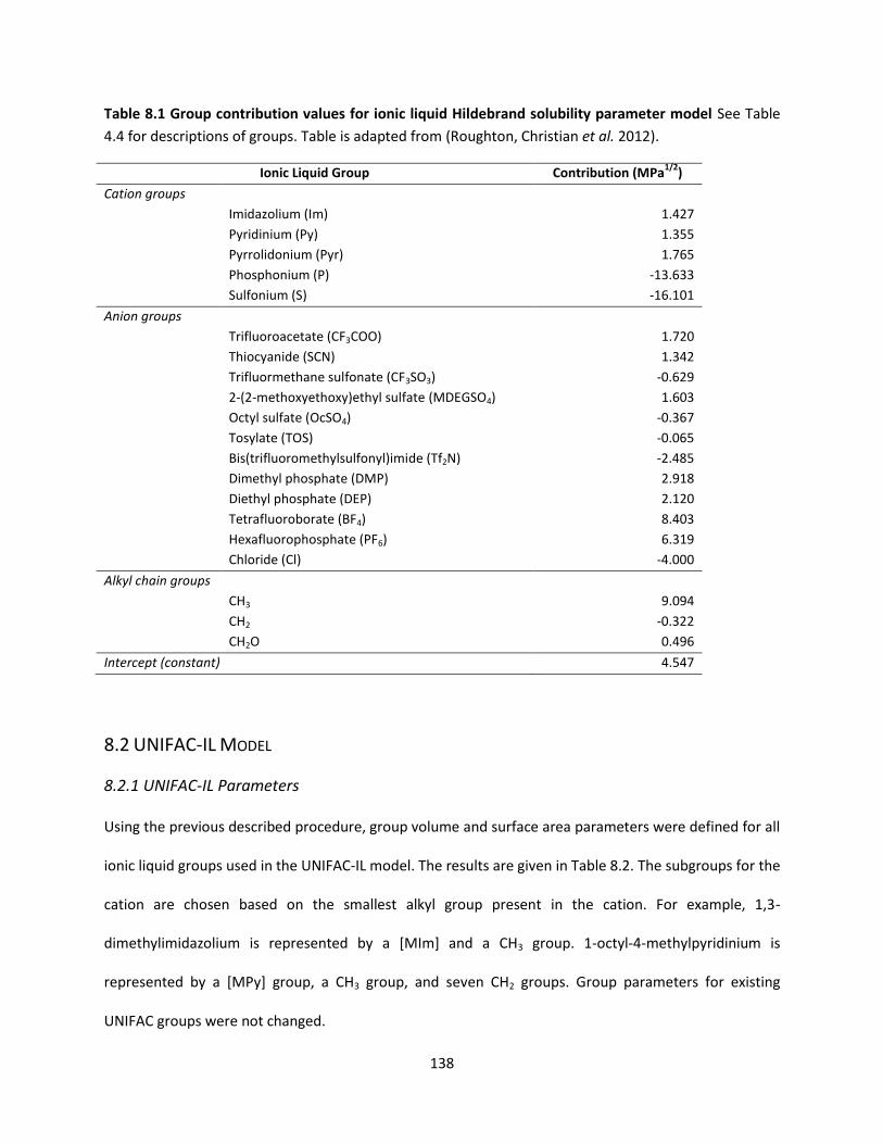
138
Table 8.1 Group contribution values for ionic liquid Hildebrand solubility parameter model See Table
4.4 for descriptions of groups. Table is adapted from (Roughton, Christian et al. 2012).
Ionic Liquid Group Contribution (MPa1/2
)
Cation groups
Imidazolium (Im) 1.427
Pyridinium (Py) 1.355
Pyrrolidonium (Pyr) 1.765
Phosphonium (P) -13.633
Sulfonium (S) -16.101
Anion groups
Trifluoroacetate (CF3COO) 1.720
Thiocyanide (SCN) 1.342
Trifluormethane sulfonate (CF3SO3) -0.629
2-(2-methoxyethoxy)ethyl sulfate (MDEGSO4) 1.603
Octyl sulfate (OcSO4) -0.367
Tosylate (TOS) -0.065
Bis(trifluoromethylsulfonyl)imide (Tf2N) -2.485
Dimethyl phosphate (DMP) 2.918
Diethyl phosphate (DEP) 2.120
Tetrafluoroborate (BF4) 8.403
Hexafluorophosphate (PF6) 6.319
Chloride (Cl) -4.000
Alkyl chain groups
CH3 9.094
CH2 -0.322
CH2O 0.496
Intercept (constant) 4.547
8.2 UNIFAC-IL MODEL
8.2.1 UNIFAC-IL Parameters
Using the previous described procedure, group volume and surface area parameters were defined for all
ionic liquid groups used in the UNIFAC-IL model. The results are given in Table 8.2. The subgroups for the
cation are chosen based on the smallest alkyl group present in the cation. For example, 1,3-
dimethylimidazolium is represented by a [MIm] and a CH3 group. 1-octyl-4-methylpyridinium is
represented by a [MPy] group, a CH3 group, and seven CH2 groups. Group parameters for existing
UNIFAC groups were not changed.
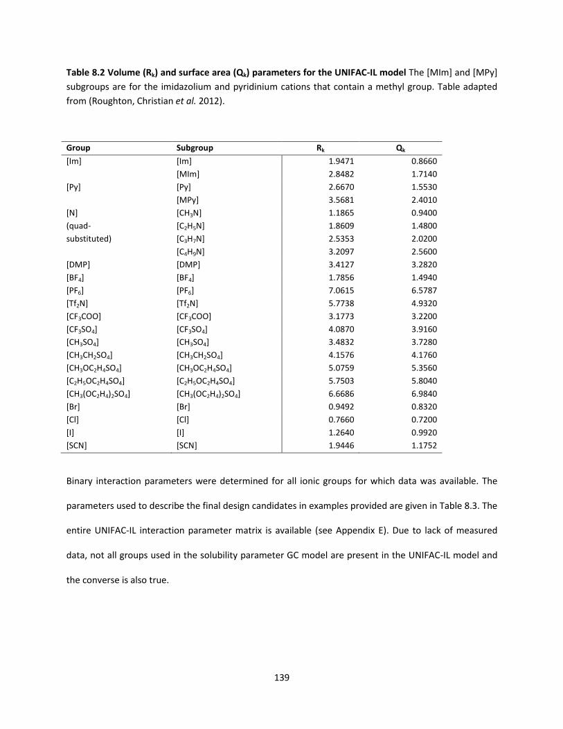
139
Table 8.2 Volume (Rk) and surface area (Qk) parameters for the UNIFAC-IL model The [MIm] and [MPy]
subgroups are for the imidazolium and pyridinium cations that contain a methyl group. Table adapted
from (Roughton, Christian et al. 2012).
Group Subgroup Rk Qk
[Im] [Im] 1.9471 0.8660
[MIm] 2.8482 1.7140
[Py] [Py] 2.6670 1.5530
[MPy] 3.5681 2.4010
[N] [CH3N] 1.1865 0.9400
(quad- [C2H5N] 1.8609 1.4800
substituted) [C3H7N] 2.5353 2.0200
[C4H9N] 3.2097 2.5600
[DMP] [DMP] 3.4127 3.2820
[BF4] [BF4] 1.7856 1.4940
[PF6] [PF6] 7.0615 6.5787
[Tf2N] [Tf2N] 5.7738 4.9320
[CF3COO] [CF3COO] 3.1773 3.2200
[CF3SO4] [CF3SO4] 4.0870 3.9160
[CH3SO4] [CH3SO4] 3.4832 3.7280
[CH3CH2SO4] [CH3CH2SO4] 4.1576 4.1760
[CH3OC2H4SO4] [CH3OC2H4SO4] 5.0759 5.3560
[C2H5OC2H4SO4] [C2H5OC2H4SO4] 5.7503 5.8040
[CH3(OC2H4)2SO4] [CH3(OC2H4)2SO4] 6.6686 6.9840
[Br] [Br] 0.9492 0.8320
[Cl] [Cl] 0.7660 0.7200
[I] [I] 1.2640 0.9920
[SCN] [SCN] 1.9446 1.1752
Binary interaction parameters were determined for all ionic groups for which data was available. The
parameters used to describe the final design candidates in examples provided are given in Table 8.3. The
entire UNIFAC-IL interaction parameter matrix is available (see Appendix E). Due to lack of measured
data, not all groups used in the solubility parameter GC model are present in the UNIFAC-IL model and
the converse is also true.
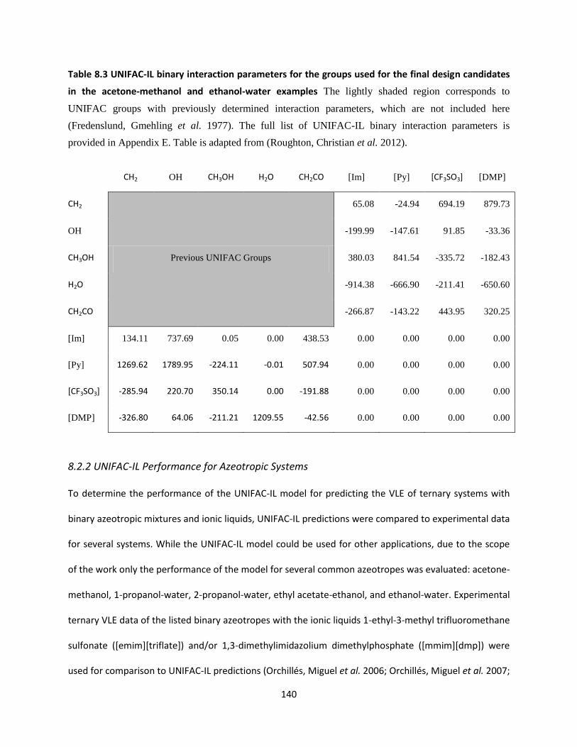
140
Table 8.3 UNIFAC-IL binary interaction parameters for the groups used for the final design candidates
in the acetone-methanol and ethanol-water examples The lightly shaded region corresponds to
UNIFAC groups with previously determined interaction parameters, which are not included here
(Fredenslund, Gmehling et al. 1977). The full list of UNIFAC-IL binary interaction parameters is
provided in Appendix E. Table is adapted from (Roughton, Christian et al. 2012).
CH2 OH CH3OH H2O CH2CO [Im] [Py] [CF3SO3] [DMP]
CH2
Previous UNIFAC Groups
65.08 -24.94 694.19 879.73
OH -199.99 -147.61 91.85 -33.36
CH3OH 380.03 841.54 -335.72 -182.43
H2O -914.38 -666.90 -211.41 -650.60
CH2CO -266.87 -143.22 443.95 320.25
[Im] 134.11 737.69 0.05 0.00 438.53 0.00 0.00 0.00 0.00
[Py] 1269.62 1789.95 -224.11 -0.01 507.94 0.00 0.00 0.00 0.00
[CF3SO3] -285.94 220.70 350.14 0.00 -191.88 0.00 0.00 0.00 0.00
[DMP] -326.80 64.06 -211.21 1209.55 -42.56 0.00 0.00 0.00 0.00
8.2.2 UNIFAC-IL Performance for Azeotropic Systems
To determine the performance of the UNIFAC-IL model for predicting the VLE of ternary systems with
binary azeotropic mixtures and ionic liquids, UNIFAC-IL predictions were compared to experimental data
for several systems. While the UNIFAC-IL model could be used for other applications, due to the scope
of the work only the performance of the model for several common azeotropes was evaluated: acetone-
methanol, 1-propanol-water, 2-propanol-water, ethyl acetate-ethanol, and ethanol-water. Experimental
ternary VLE data of the listed binary azeotropes with the ionic liquids 1-ethyl-3-methyl trifluoromethane
sulfonate ([emim][triflate]) and/or 1,3-dimethylimidazolium dimethylphosphate ([mmim][dmp]) were
used for comparison to UNIFAC-IL predictions (Orchillés, Miguel et al. 2006; Orchillés, Miguel et al. 2007;

141
Orchill s, Miguel et al. 2008; Orchill s, Miguel et al. 2010; Wang, Wang et al. 2010). Figures 8.2-8.7 show
the comparison between the UNIFAC-IL predictions and experimental data, where component (1) is the
light component and is listed first in the figure caption.
Figure 8.2 Acetone-methanol-[emim][triflate] x-y diagram at 100 kPa 6.0 mol% ionic liquid is present.
The dashed line indicates the UNIFAC-IL prediction and the open circles represent experimental data
(Orchillés, Miguel et al. 2006). 6.84 %AARD was observed between the experimental and predicted
vapor fractions. Figure adapted from (Roughton, Christian et al. 2012).
Figure 8.3 1-propanol-water-[emim][triflate] x-y diagram at 100 kPa 6.0 mol% ionic liquid is present.
The dashed line indicates the UNIFAC-IL prediction and the open circles represent experimental data
(Orchill s, Miguel et al. 2008). 10.84 %AARD was observed between the experimental and predicted
vapor fractions. Figure adapted from (Roughton, Christian et al. 2012).
0
0.1
0.2
0.3
0.4
0.5
0.6
0.7
0.8
0.9
1
0 0.1 0.2 0.3 0.4 0.5 0.6 0.7 0.8 0.9 1
y1
x1 (IL-free basis)
0
0.1
0.2
0.3
0.4
0.5
0.6
0.7
0.8
0.9
1
0 0.1 0.2 0.3 0.4 0.5 0.6 0.7 0.8 0.9 1
y1
x1 (IL-free basis)

142
Figure 8.4 Ethyl acetate-ethanol-[emim][triflate] x-y diagram at 100 kPa 6.0 mol% ionic liquid is
present. The dashed line indicates the UNIFAC-IL prediction and the open circles represent experimental
data (Orchillés, Miguel et al. 2007). 7.93 %AARD was observed between the experimental and predicted
vapor fractions. Figure adapted from (Roughton, Christian et al. 2012).
Figure 8.5 Ethanol-water-[emim][triflate] x-y diagram at 100 kPa 6.0 mol% ionic liquid is present. The
dashed line indicates the UNIFAC-IL prediction and the open circles represent experimental data
(Orchill s, Miguel et al. 2010). 6.45 %AARD was observed between the experimental and predicted
vapor fractions. Figure adapted from (Roughton, Christian et al. 2012).
0
0.1
0.2
0.3
0.4
0.5
0.6
0.7
0.8
0.9
1
0 0.1 0.2 0.3 0.4 0.5 0.6 0.7 0.8 0.9 1
y1
x1 (IL-free basis)
0
0.1
0.2
0.3
0.4
0.5
0.6
0.7
0.8
0.9
1
0 0.1 0.2 0.3 0.4 0.5 0.6 0.7 0.8 0.9 1
y1
x1 (IL-free basis)

143
Figure 8.6 1-propanol-water-[mmim][dmp] P-T diagram x1 = 0.6669 and x2 = 0.2472. The solid line
indicates the UNIFAC-IL prediction and the open circles represent experimental data (Wang, Wang et al.
2010). 1.10 %AARD was observed between the experimental and predicted total pressures. Figure
adapted from (Roughton, Christian et al. 2012).
Figure 8.7 2-propanol- water-[mmim][dmp] P-T diagram x1 = 0.6669 and x2 = 0.2472. The solid line
indicates the UNIFAC-IL prediction and the open circles represent experimental data (Wang, Wang et al.
2010). 1.34 %AARD was observed between the experimental and predicted total pressures. Figure
adapted from (Roughton, Christian et al. 2012).
Overall, the UNIFAC-IL model shows good prediction of the experimentally observed VLE. As the
experimental data used for model evaluation was not used to regress the UNIFAC-IL parameters,
0
20
40
60
80
100
120
140
320 330 340 350 360 370 380
P [
kPa]
T [K]
0
20
40
60
80
100
120
140
300 310 320 330 340 350 360 370
P [
kPa]
T [K]

144
agreement between the model and experiments was not assured. The largest AARD between the
experimental and predicted vapor composition values is observed for the 1-propanol-water-
[emim][triflate] system with a value of 10.84%. The UNIFAC-IL predictions of azeotrope existence and
location agree very well with the experimental data. Qualitatively, the shapes of the x-y curves are
similar when comparing the UNIFAC-IL predictions and the experimental data. The P-T predictions
showed very good agreement with experimental data, with the largest AARD value of 1.34% observed
for the 2-propanol- water-[mmim][dmp] system. While the comparison to experimental data is limited,
the results indicate that the UNIFAC-IL model will provide reasonable predictions for the azeotropes
considered for simultaneous ionic liquid and separation process design. The two ionic liquids present in
the experimental data are similar (or the same for [mmim][dmp]) to the designed ionic liquids for both
azeotrope examples, suggesting that the UNIFAC-IL predictions for the designed ionic liquids will be
reasonably accurate.
8.3 CAMD RESULTS FOR IONIC LIQUID ENTRAINERS
Ionic liquid entrainers were designed for use with both the acetone-methanol and ethanol-water
azeotropes. Candidates were found that either best matched the volume average solubility parameter
value of each azeotropic mixture or the solubility parameter of the desired entrained component. The
cation choices were limited to imidazolium and pyridinium to ensure that the designed ionic liquid could
be used with the UNFAC-IL model. With the groups determined by CAMD, the groups were then
constructed to make a feasible ionic liquid. The design candidates for the acetone-methanol azeotrope
were 1-octyl-4-methylpyridinium trifluoromethane sulfonate ([ompy][triflate]) with a solubility
parameter value of 21.2 MPa1/2 and 1-butyl-3-methylimidazolium hexafluorophosphate ([bmim][PF6])
with a solubility parameter value of 29.5 MPa1/2. 1,3-dimethylimidazolium dimethylphosphate
([mmim][dmp]) with a solubility parameter value of 27.1 MPa1/2 and 1,3-dimethylimidazolium
145
tetrafluoroborate ([mmim][BF4]) with a solubility parameter value of 32.6 MPa1/2 were the design
candidates for the ethanol-water azeotrope.
The UNIFAC-IL model was used to ensure that the azeotropes were broken by the designed ionic liquids
and that the correct component was entrained by the ionic liquid. Existence of only one liquid phase was
confirmed by the UNIFAC-IL model. The UNIFAC-IL model was also used to predict the minimum amount
of ionic liquid needed to break the azeotrope at 101.325 kPa. The ionic liquid 1-ethyl-3-methyl
trifluoromethane sulfonate ([emim][triflate]) has been shown experimentally to break both the acetone-
methanol and ethanol-water azeotropes (Orchillés, Miguel et al. 2006; Orchill s, Miguel et al. 2010).
Based on the predicted solubility parameter, [emim][triflate] would not be designed using the CAMD
procedure for both azeotropes. The UNIFAC-IL model was used to predict the minimum amount of
[emim][triflate] needed to break both azeotropes at 101.325 kPa. VLE calculations were used to
calculate vapor compositions of components for each liquid composition for increasing ionic liquid
concentrations from no ionic liquid present to the concentration where the azeotrope is just broken,
defined as the minimum ionic liquid concentration needed to break the azeotrope. The ionic liquid
composition was increased by 0.01 mol% and calculations were performed at each composition. The
minimum ionic liquid concentrations required were used to screen the design candidates. For acetone-
methanol, slightly more [emim][triflate] on a mole fraction basis was needed to break the azeotropes
when compared to the designed ionic liquid [ompy][triflate]. The designed ionic liquid [bmim][PF6]
required a much higher concentration to break the acetone-methanol azeotrope when compared to the
other design candidate and was eliminated from further consideration. Approximately the same amount
of the design candidates [mmim][dmp] and [mmim][BF4] were needed to break the ethanol-water
azeotrope, so both ionic liquids were keep as entrainer candidates. The experimentally selected ionic
liquid [emim][triflate] broke the ethanol-water azeotrope at a similar concentration to that of the design
candidates. The results are summarized in Table 5. To illustrate the performance of the designed ionic

146
liquid candidates and the experimentally selected ionic liquid, Figures 8.8 and 8.9 show the x-y diagrams
for the acetone-methanol and ethanol-water systems with 10 mol% of each considered ionic liquid
added. The candidate [ompy][triflate] shows much higher vapor mole fractions than the candidate
[bmim][PF6] at any given liquid mole fraction, indicating that [ompy][triflate] generates noticeably
higher driving forces (y1 – x1) for separation. The driving forces generated by [ompy][triflate] are also
slightly higher than the driving forces generated by the experimentally selected ionic liquid
[emim][triflate]. For the ethanol-water system, both the candidate ionic liquids and the experimentally
selected ionic liquid showed similar driving forces.
Figure 8.8 x-y diagram showing the performance of several ionic liquid entrainers on the acetone-methanol azeotrope at 101.325 kPa The concentration of all ionic liquid entrainers is set a 10 mol%. The
45 degree line is included to indicate where y1 = x1. Figure adapted from (Roughton, Christian et al.
2012).
0.7
0.75
0.8
0.85
0.9
0.95
1
0.7 0.75 0.8 0.85 0.9 0.95 1
y1
x1
No IL
[emim][triflate]
[bmim][PF6]
[ompy][triflate]

147
Figure 8.9 x-y diagram showing the performance of several ionic liquid entrainers on the ethanol-water azeotrope at 101.325 kPa The concentration of all ionic liquid entrainers is set a 10 mol%. The 45
degree line is included to indicate where y1 = x1. Figure adapted from (Roughton, Christian et al. 2012).
By designing the ionic liquid entrainer based on solubility parameter targets and screening based on the
amount needed to break the azeotrope, ionic liquid candidates were identified that required minimal
concentrations to break a given azeotrope. By requiring less ionic liquid, material inputs are reduced and
energy requirements are reduced as less ionic liquid needs to be recovered. The ionic liquid
[emim][triflate] appears to be a good candidate for breaking the ethanol-water azeotrope but does not
have a predicted solubility parameter value that lies within the range of solubility parameter values that
would be considered for the initial design step in the CAMD procedure. Although [emim][triflate] would
not be chosen through the design process, the designed candidates both break the ethanol-water
azeotrope with the same or similar minimum concentration. Design of ionic liquids for the example
systems provided ionic liquid candidates that could break the azeotropes with concentrations less than
or equal to the concentration of the experimentally selected ionic liquid [emim][triflate].
0.7
0.75
0.8
0.85
0.9
0.95
1
0.7 0.75 0.8 0.85 0.9 0.95 1
y1
x1
No IL
[emim][triflate]
[mmim][BF4]
[mmim][DMP]

148
Tab
le 8
.4 C
om
par
iso
n o
f m
inim
um
am
ou
nt
of
des
ign
ed
an
d e
xpe
rim
en
tally
se
lect
ed
ion
ic li
qu
ids
req
uir
ed t
o b
reak
th
e ac
eto
ne
-me
than
ol
and
eth
ano
l-w
ate
r az
eo
tro
pe
s at
10
1.3
25
kP
a P
red
icti
on
s w
ere
mad
e u
sin
g U
NIF
AC
-IL
mo
del
. Tab
le a
dap
ted
fro
m (
Ro
ugh
ton
, Ch
rist
ian
et
al.
20
12
).

149
8.4 DESIGN OF IONIC LIQUID-BASED AZEOTROPIC SEPARATION PROCESSES
Using the outlined procedure and specifications, distillation columns for the azeotrope mixtures were
designed using both designed ionic liquid candidates and an experimentally selected ionic liquid. At a
given ionic liquid flow rate, the minimum amount of stages needed to achieve the specified separation
was determined. The driving force method with the proposed modified scaling was used an initial guess
for the feed stage. The feed stage was then moved up and down to find the optimal feed stage in terms
of energy requirements. In all cases, the optimal feed stage was at or near the feed stage proposed by
the driving force method. The results for the ethanol-water-[mmim][dmp] system are given by Figure
8.10. The results indicate that use of the driving force method with the new proposed scaling can be
used to design optimal or near-optimal distillation columns with a main feed and separate ionic liquid
feed. The driving force method was originally proposed for a distillation column with only one feed. By
comparing the columns with optimal feed stages at different ionic liquid flow rates, the flow rate and
column configuration yielding the minimum stages and energy requirements was obtained for each
system. The results for the ethanol-water-[mmim][dmp] system are given by Figure 8.11.
From the simulation results, optimal distillation columns in regards to minimal stages required and
energy inputs were obtained for the methanol-acetone and ethanol-water systems using either
designed entrainer candidates or an experimentally selected ionic liquid entrainer. The results are
summarized in Table 8.5.

150
Figure 8.10 Reboiler heat duty as a function of feed stage location for separation of the ethanol-water azeotrope using various amounts of [mmim][dmp] as an entrainer The scaled feed stage location
calculated by the driving force method is circled in the figure for each ionic liquid feed rate. The lines are
drawn to guide the eyes. Figure adapted from (Roughton, Christian et al. 2012).
Figure 8.11 Reboiler heat duty as a function of ionic liquid flow rate for separation of the ethanol-water azeotrope using [mmim][dmp] as an entrainer Each point indicates the optimal column
configuration in terms of energy requirements for the specified ionic liquid flow rate. The line is drawn
to guide the eyes. Figure adapted from (Roughton, Christian et al. 2012).
1,750
2,000
2,250
2,500
2,750
3,000
3,250
3,500
3,750
4,000
4 5 6 7 8 9 10 11
Re
bo
iler
Du
ty [
kW]
Feed Stage Location (N = 16)
22.2 kmol/hr
25 kmol/hr
30 kmol/hr
35 kmol/hr
40 kmol/hr
1,500
2,000
2,500
3,000
3,500
4,000
20 25 30 35 40 45 50 55
Re
bo
iler
Du
ty [
kW]
[mmim][dmp] flowrate (kmol/hr)
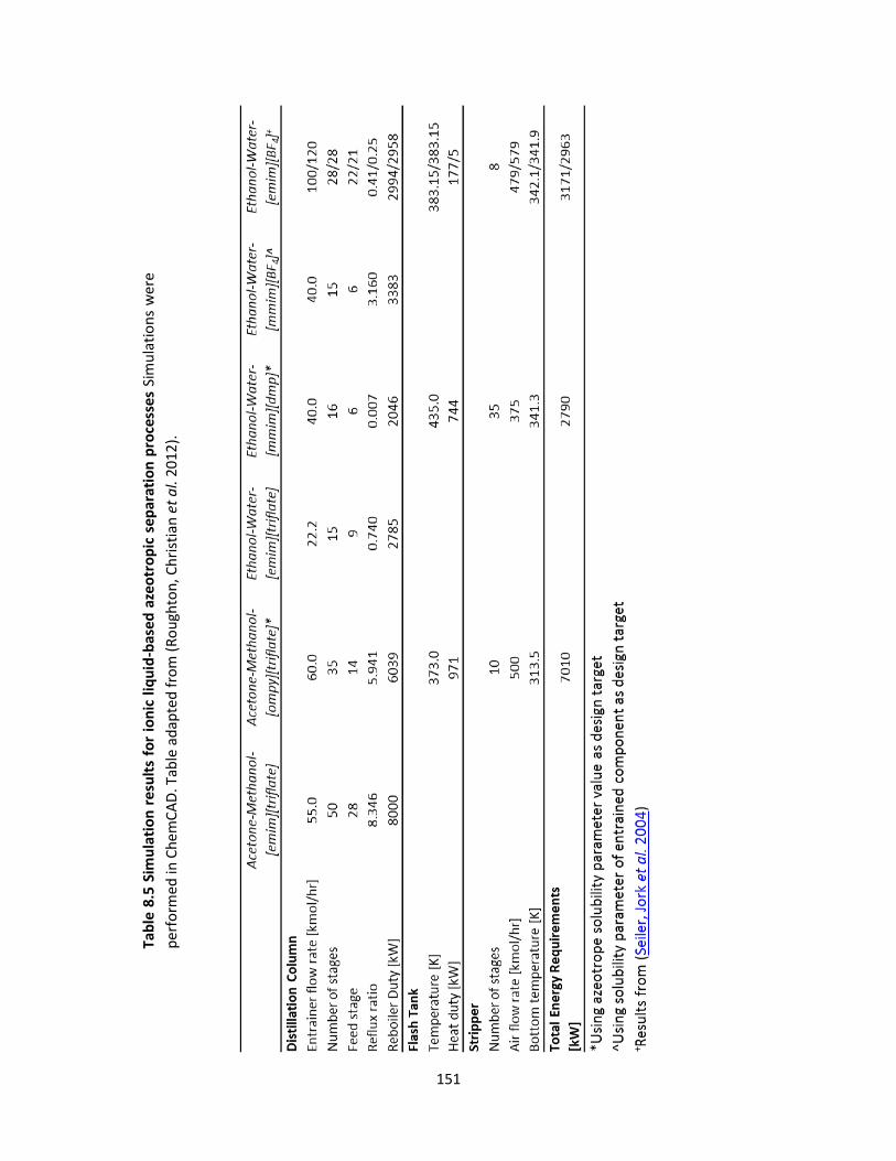
151
Tab
le 8
.5 S
imu
lati
on
res
ult
s fo
r io
nic
liq
uid
-bas
ed
aze
otr
op
ic s
ep
arat
ion
pro
cess
es S
imu
lati
on
s w
ere
per
form
ed in
Ch
emC
AD
. Tab
le a
dap
ted
fro
m (
Ro
ugh
ton
, Ch
rist
ian
et
al.
20
12
).
152
For both systems, a designed ionic liquid was found to have significant energy savings in comparison to
the experimentally selected ionic liquid. Based on the column simulation results, the ionic liquid
candidates with the lowest energy requirements were kept and the other candidates were eliminated.
The ionic liquid flow rates used in the simulation were selected based on minimizing energy
requirements, resulting in different flow rates for the different ionic liquids. While the experimentally
selected ionic liquid used lower flow rates, the energy requirements were higher for both azeotropic
systems when compared to the final design candidates. For acetone-methanol, use of [ompy][triflate]
provided the lowest energy requirements and reduced energy consumption by 24.5% (1961 kW)
compared to the experimentally selected ionic liquid [emim][triflate]. As no other design candidate
remained, [ompy][triflate] was selected as the final design candidate for the acetone-methanol system.
Energy requirements for the ethanol-water system were lowest when using [mmim][dmp], reducing
heat duty by 26.5% (739 kW) when compared to the experimentally selected ionic liquid
[emim][triflate]. As the column using [mmim][dmp] required less energy than the other design
candidate [mmim][BF4], [mmim][dmp] was chosen as the final design candidate and [mmim][BF4] was
eliminated from consideration. Both [ompy][triflate] (Papaiconomou, Salminen et al. 2007) and
[mmim][dmp] (Wang, Wang et al. 2010) have been previously synthesized and studied. The structures
of [ompy][triflate] and [mmim][dmp] are shown in Figure 8.12 and Figure 8.13.
The column energy requirements were closer in value for the ethanol-water system than the acetone-
methanol system, likely influenced by the fact that [mmim][dmp], [mmim][BF4], and [emim][triflate]
have similar maximum driving force values at the ionic liquid concentrations used. The minimum
number of stages needed for the separation was found to be less for the methanol-acetone system
using the designed ionic liquid than found when using the experimentally selected ionic liquid. The
experimentally selected ionic liquid was able to achieve separation in one less stage than the final ionic
liquid design candidate for the ethanol-water system, but the reduced capital cost would not offset the

153
larger energy requirement. Due to the energy savings, the entire process including entrainer
regeneration was simulated only for the systems using the final design candidate entrainers. The energy
required for air flow into the stripper was neglected in calculation of the total energy requirements for
the processes.
Figure 8.12 1-octyl-4-methylpyridinium trifluoromethane sulfonate ([ompy][triflate]) With a solubility
parameter value of 21.2 MPa1/2, the ionic liquid is the final design candidate for the acetone-methanol
azeotrope.
Figure 8.13 1,3-dimethylimidazolium dimethylphosphate ([mmim][dmp]) With a solubility parameter
value of 27.1 MPa1/2, the ionic liquid is the final design candidate for the ethanol-water azeotrope.
The results for the ethanol-water-[mmim][dmp] system were compared to previously published
simulation results for ethanol-water separation using a conventional entrainer (1,2-ethanediol) and a
experimentally selected ionic liquid entrainer (1-ethyl-3-methylimidazolium tetrafluoroborate
[emim][BF4]) (Seiler, Jork et al. 2004). The results for the experimentally selected ionic liquid are

154
compared to the results for the designed ionic liquid candidates in Table 8.5. The separation process was
the same as used in the current work and the number of stages in the distillation column was set at 28
for both the conventional and ionic liquid entrainers. Simulations were performed to calculate energy
requirements at various entrainer concentrations. The optimal energy requirements were 3917 kW for
the conventional entrainer and 2963 kW for the ionic liquid (Seiler, Jork et al. 2004). Comparison of the
separation processes shows an energy savings of 28.8% (1127 kW) when using [mmim][dmp] instead of
the conventional entrainer and an energy savings of 5.8% (173 kW) when using [mmim][dmp] over an
experimentally selected ionic liquid. Due to inherent error in the UNIFAC-IL model, the calculated excess
enthalpies may result in some error in the calculated energy requirements. Use of ionic liquids offers an
alternative to conventional entrainers which may reduce energy requirements when separating
azeotropic mixtures. By designing the ionic liquid structure to match a solubility parameter target range
and further screening candidates by minimum concentration needed to break the azeotrope and column
energy requirements, energy requirements in the resulting separation and entrainer regeneration
processes are reduced compared to processes using ionic liquids that were not designed or selected
using a CAMD procedure.
8.5 PREDICTION OF RELEVANT PROPERTIES FOR IN SITU EXTRACTIVE FERMENTATION
The data sets used to generate the models for partition coefficient of NDHD in ionic liquid (Kx) and
toxicity of ionic liquid towards E. coli (lnEC50) were too small to allow descriptor selection through use of
Mallow’s Cp. Alternatively, models were compared using the based on R2-Q2 value, with the model
showing the minimum value being selected. R2-Q2 provides a measure of the difference between the fit
and the predictive capability. Minimal differences are desired.
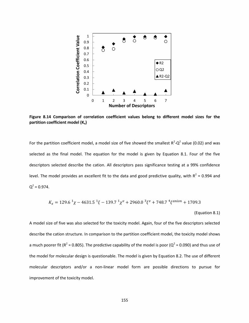
155
Figure 8.14 Comparison of correlation coefficient values belong to different model sizes for the partition coefficient model (Kx)
For the partition coefficient model, a model size of five showed the smallest R2-Q2 value (0.02) and was
selected as the final model. The equation for the model is given by Equation 8.1. Four of the five
descriptors selected describe the cation. All descriptors pass significance testing at a 99% confidence
level. The model provides an excellent fit to the data and good predictive quality, with R2 = 0.994 and
Q2 = 0.974.
(Equation 8.1)
A model size of five was also selected for the toxicity model. Again, four of the five descriptors selected
describe the cation structure. In comparison to the partition coefficient model, the toxicity model shows
a much poorer fit (R2 = 0.805). The predictive capability of the model is poor (Q2 = 0.090) and thus use of
the model for molecular design is questionable. The model is given by Equation 8.2. The use of different
molecular descriptors and/or a non-linear model form are possible directions to pursue for
improvement of the toxicity model.
0
0.1
0.2
0.3
0.4
0.5
0.6
0.7
0.8
0.9
1
0 1 2 3 4 5 6 7
Co
rrel
atio
n C
oef
fici
ent
Val
ue
Number of Descriptors
R2
Q2
R2-Q2
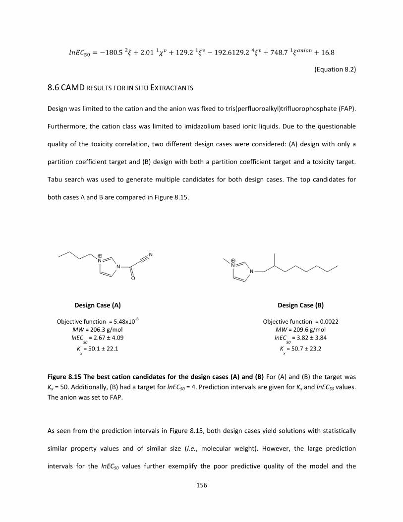
156
(Equation 8.2)
8.6 CAMD RESULTS FOR IN SITU EXTRACTANTS
Design was limited to the cation and the anion was fixed to tris(perfluoroalkyl)trifluorophosphate (FAP).
Furthermore, the cation class was limited to imidazolium based ionic liquids. Due to the questionable
quality of the toxicity correlation, two different design cases were considered: (A) design with only a
partition coefficient target and (B) design with both a partition coefficient target and a toxicity target.
Tabu search was used to generate multiple candidates for both design cases. The top candidates for
both cases A and B are compared in Figure 8.15.
Design Case (A) Design Case (B)
Objective function = 5.48x10⁻⁶
Objective function = 0.0022 MW = 206.3 g/mol MW = 209.6 g/mol lnEC
50 = 2.67 ± 4.09 lnEC
50 = 3.82 ± 3.84
Kx = 50.1 ± 22.1 K
x = 50.7 ± 23.2
Figure 8.15 The best cation candidates for the design cases (A) and (B) For (A) and (B) the target was
Kx = 50. Additionally, (B) had a target for lnEC50 = 4. Prediction intervals are given for Kx and lnEC50 values.
The anion was set to FAP.
As seen from the prediction intervals in Figure 8.15, both design cases yield solutions with statistically
similar property values and of similar size (i.e., molecular weight). However, the large prediction
intervals for the lnEC50 values further exemplify the poor predictive quality of the model and the

157
corresponding predictions are likely to be unreliable. Of interest is the observation that the inclusion of
toxicity as a target prevented any polar groups from being included in the alkyl chain of the cation,
where polar groups are present when only partition coefficient was used as a target.
158
9.0 RESULTS FOR LYOPHILIZED EXCIPIENT DESIGN
The following section presents the results for property models developed for CAMD of lyophilized
excipients. Also included are the tuning and design results for the CAMD methods considered. Two main
approaches were used to design excipients for lyophilized protein formulations: a vitrification approach
with optimal glass transition temperatures and an overall reduction of aggregation approach to maintain
%Monomer at 100% following lyophilization.
Section 9.1 presents the model results for various glass transition correlations. The molecular design
results using tabu search are presented in Section 9.2. The experimental measurements observed for
protein loss following lyophilization are detailed in Section 9.3. Sections 9.4-9.6 present and discuss the
results for various post-lyophilization protein loss models. The tuning results for both tabu search and a
genetic algorithm are given in Section 9.7. Finally, Section 9.8 contains the molecular design results
using the post-lyophilization protein loss models with the tuned stochastic algorithms. Results are
compared between optimization methods and also between the proteins included in the formulation.
9.1 GLASS TRANSITION TEMPERATURE PROPERTY MODELS
The R statistical program (R-Development-Core-Team 2010) was used for linear regression of the
desired properties to the connectivity indices of the excipients in the training set. The model data was
obtained from literature (Roos 1993). The carbohydrate excipients used in the model data set were
monosaccharides (ribose, xylose, fructose, fucose, glucose, and sorbose), disaccharides (lactose,
lactulose, melibiose, sucrose, and trehalose), oligosaccharides (raffinose), and sugar alcohols (maltitol,
sorbitol, and xylitol). The leaps package in R (Lumley 2004) was used to conduct an exhaustive search to
determine which combination of descriptors provided the lowest Cp value for each number of possible
descriptors that could be used for the QSPR (ranging from one to twelve). A summary of the QSPRs

159
developed in this work is provided in Table 9.1. The individual QSPRs are further detailed in the
following subsections.
Table 9.1 Summary of glass transition-related QSPRs developed Figure adapted from (Roughton, Topp
et al. 2012).
QSPR Number of Descriptors Selected R2
Tg 9 0.998
Tg’ 6 0.994
Tm’ 7 0.997
k 9 0.998
9.1.1 QSPR for Glass Transition Temperature of Anhydrous Solute
The glass transition temperature of the anhydrous solute provides an indication of the stability of the
carbohydrate excipient during storage conditions. In addition to being used as a criterion for storage
stability, Tg is used in the calculation of the excipient concentration in a maximally freeze-concentrated
matrix.
The correlation developed for the Tg of carbohydrate excipients is:
( )
(Equation 9.1)
Equation 9.1 provides a good fit for the experimental measurements, providing a coefficient of
determination (R2) value of 0.998. The predicted Tg values are compared to the experimental values
using a parity plot in Figure 9.1.

160
Figure 9.1 Comparison of measured experimental values to QSPR predicted values for the glass transition temperature of the anhydrous solute (Tg) The y=x line indicates were predicted =
experimental. Figure adapted from (Roughton, Topp et al. 2012).
9.1.2 QSPR for Glass Transition Temperature of Maximally Concentrated Solute
In addition to being used as a criterion for ensuring formation of a maximally freeze-concentrated glass
matrix, the glass transition temperature of the maximally concentrated solute (Tg’) is used in the
calculation of the excipient concentration in the glass matrix.
The correlation developed for the Tg’ of carbohydrate excipients is:
( )
(Equation 9.2)
Equation 9.2 provides a good fit for the experimental measurements, providing an R2 value of 0.994. The
predicted Tg’ values are compared to the experimental values using a parity plot in Figure 9.2.
-40
-20
0
20
40
60
80
100
-40 -20 0 20 40 60 80 100
Pre
dic
ted
Val
ue
(°C
)
Experimental Value (°C)

161
Figure 9.2 Comparison of measured experimental values to QSPR predicted values for the glass transition temperature of the maximally freeze-concentrated solute (Tg’) The y=x line indicates were
predicted = experimental. Figure adapted from (Roughton, Topp et al. 2012).
9.1.3 QSPR for the Melting Point of Ice
The melting point of ice represents the onset of ice formation during the freezing part of the
lyophilization process. The concentrated solution must be annealed between Tg’ and Tm’ to ensure that
the resulting freeze-concentrated glass matrix is maximally concentrated.
The correlation developed for the Tm’ of carbohydrate excipients is given below:
( )
(Equation 9.3)
Equation 9.3 provides a good fit for the experimental measurements, providing an R2 value of 0.997. The
predicted Tm’ values are compared to the experimental values using a parity plot in Figure 9.3.
-80
-75
-70
-65
-60
-55
-50
-45
-40
-35
-30
-80 -75 -70 -65 -60 -55 -50 -45 -40 -35 -30
Pre
dic
ted
Val
ue
(°C
)
Experimental Value (°C)
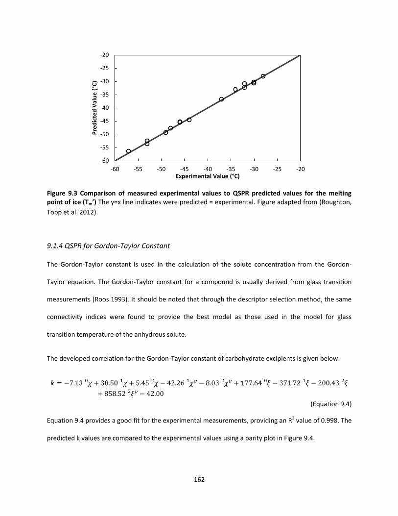
162
Figure 9.3 Comparison of measured experimental values to QSPR predicted values for the melting point of ice (Tm’) The y=x line indicates were predicted = experimental. Figure adapted from (Roughton,
Topp et al. 2012).
9.1.4 QSPR for Gordon-Taylor Constant
The Gordon-Taylor constant is used in the calculation of the solute concentration from the Gordon-
Taylor equation. The Gordon-Taylor constant for a compound is usually derived from glass transition
measurements (Roos 1993). It should be noted that through the descriptor selection method, the same
connectivity indices were found to provide the best model as those used in the model for glass
transition temperature of the anhydrous solute.
The developed correlation for the Gordon-Taylor constant of carbohydrate excipients is given below:
(Equation 9.4)
Equation 9.4 provides a good fit for the experimental measurements, providing an R2 value of 0.998. The
predicted k values are compared to the experimental values using a parity plot in Figure 9.4.
-60
-55
-50
-45
-40
-35
-30
-25
-20
-60 -55 -50 -45 -40 -35 -30 -25 -20
Pre
dic
ted
Val
ue
(°C
)
Experimental Value (°C)

163
Figure 9.4 Comparison of measured experimental values to QSPR predicted values for the Gordon-Taylor constant (k) The y=x line indicates were predicted = experimental. Figure adapted from
(Roughton, Topp et al. 2012).
9.2 RESULTS FOR OPTIMAL GLASS FORMER DESIGN
According to vitrification theory, a protein stabilizing excipient should be able to form a glass during
lyophilization and subsequent storage of the therapeutic product. The glass transition temperature of
the maximally freeze-concentrated solute and the melting point of ice for a carbohydrate excipient must
be high enough to be feasibly reached during the lyophilization process. The protein drug product must
first be annealed at a temperature between Tg’ and Tm and then reduced below Tg’ to yield a maximally
freeze-concentrated matrix (Roos 1997). The melting temperature of ice is higher than the glass
transition temperature of the maximally concentrated solute. The glass transition temperature of the
anhydrous solute must be sufficiently high such that the carbohydrate remains a glass during storage of
the protein drug product. A common heuristic is that the storage temperature of an amorphous drug
formulation should be 50°C below the anhydrous glass transition temperature (Costantino and Pikal
2004). For a formulation to be stored at room temperature, a Tg of at least 80°C is desired. This criterion
is very important, as more than 70% of commercial lyophilized products cannot be stored at room
2
2.5
3
3.5
4
4.5
5
5.5
6
6.5
7
2 2.5 3 3.5 4 4.5 5 5.5 6 6.5 7
Pre
dic
ted
Val
ue
(D
ime
nsi
on
less
)
Experimental Value (Dimensionless)

164
temperature and must be refrigerated to maintain stability, complicating the use of the drugs
(Costantino and Pikal 2004). All three phase transition temperatures are used along with the Gordon-
Taylor constant to determine the excipient concentration (weight fraction) of a maximally freeze-
concentrated matrix, without protein present. A higher excipient concentration corresponds to lower
residual water in the matrix, which lowers the mobility of the protein and thus reduces the potential for
aggregation. No target is placed on the actual value of the Gordon-Taylor constant. The Gordon-Taylor
constant is calculated only for use in subsequent calculation of the excipient concentration in a
maximally freeze-concentrated matrix.
Table 9.2 Property values of candidate carbohydrate excipients designed using tabu search Prediction
intervals for the properties predicted by the QSPR models were calculated at a 95% level. A lower
objective function score indicates a better match for the target property values. Table is adapted from
(Roughton, Topp et al. 2012).
Property Candidate 1 Candidate 2 Candidate 3
Tg 100.9±12.7°C 99.8±15.0°C 90.3 ± 20.6°C
Tg’ -32.6±6.5°C -33.1±6.7°C -31.7± 5.0°C
Tm’ -24.8±3.2°C -23.7±3.5°C -24.1 ± 4.1°C
k 6.76± 0.37 6.73 ± 0.44 6.46 ± 0.61
Cg’ 0.838 0.838 0.845
MW 373.3 g/mol 373.3 g/mol 373.3 g/mol
Obj function 0.00800 0.01367 0.01373
The described molecular design framework was employed using the PD program previously used to
design various molecules, including dental polymers (Eslick, Ye et al. 2009) and ionic liquids (McLeese,
Eslick et al. 2010).The results for the three best excipient candidates are given in Table 9.2, determined
by the solutions with the lowest objective function scores. Seven total candidates were generated. Error

165
was calculated using prediction integrals at a 95% level for the property values predicted using the QSPR
models. The structures of the proposed carbohydrate excipients are given in Figures 9.5-9.7.
Figure 9.5 Optimal carbohydrate excipient candidate 1 proposed by CAMD using tabu search The
objective function score is 0.00800. Figure adapted from (Roughton, Topp et al. 2012).
Figure 9.6 Optimal carbohydrate excipient candidate 2 proposed by CAMD using tabu search The
objective function score is 0.01367. Figure adapted from (Roughton, Topp et al. 2012).

166
Figure 9.7 Optimal carbohydrate excipient candidate 3 proposed by CAMD using tabu serach The
objective function score is 0.01373. Figure adapted from (Roughton, Topp et al. 2012).
The proposed excipients are similar to disaccharide and oligosaccharide molecular topologies.
Candidates 1, 2, and 3 are isomers. The property values of the proposed excipients show that the
computationally designed excipient molecules should stabilize protein formulations. Protein mobility
should be limited due to the high solute concentration of the maximally freeze-concentrated matrix. The
values for the glass transition temperature of the maximally freeze-concentrated solute and the melting
point of ice are high enough that they can be reached during lyophilization. Additionally, the gap in the
two temperatures is large enough to allow for annealing between the two temperatures, ensuring that
the maximum solute concentration is reached in the freeze-concentrated matrix. The high glass
transition temperatures of the anhydrous solute are high enough that drying and long term storage
conditions will not change the desired glass structure of the protein formulation.
The prediction intervals show that for all three candidates, all four properties predicted by the QSPR
models have overlapping prediction intervals. Due to the overlapping prediction intervals, the predicted
property values of all the candidates are not statistically different; all three candidates are valid
solutions for the optimization problem. Use of tabu search was able to provide several optimal excipient

167
candidates with statistically similar property values, where a deterministic method would have only
provided one candidate. The prediction intervals for the glass transition temperature of the anhydrous
solute were large for all three candidates. The large magnitude of the prediction interval is likely due to
the target value being close to the upper limit of the property data used to build the correlation.
One should note that since not all possible properties of importance for an excipient have been
included, these structures should be considered candidates for protein drug excipients, and not finalized
designs to be immediately utilized. Since all of the structures designed in this work are similar to
disaccharides, it is likely that they can be synthesized. However, further studies would be required to
ensure that the excipients themselves exhibit sufficient properties to be used in protein drug
formulations.
9.3 EXPERIMENTAL RESULTS FOR POST-LYOPHILIZATION PROTEIN LOSS
Experimental studies were performed in two rounds. The first round was focused on creating a dataset
for modeling %Monomer as a function of protein structure. Accordingly, a large amount of proteins
were considered and fewer excipients. The second round was focused on creating a dataset for
correlation of %Monomer to excipient structure. Therefore, a large amount of excipients were
considered with a small set of proteins.
It is noted here that the experiments for the first round were not performed by the author and were
instead conducted by Lavanya K. Iyer at Purdue University. The methods and procedures used were the
same as those used by the author and described in Section 3.0. The results and discussion arising from
the experiments is included as the data was used to build the corresponding models for %Monomer as a
function of protein structure.

168
9.3.1 Experimental Results for Data Set Concerning Protein Structure
For the fifteen proteins and five lyophilized formulations studied here, aggregation varied with protein,
with formulation and with the analytical method used to assess aggregation (see Table F.1, Appendix F).
The proteins can be grouped according to aggregation tendency. Five proteins (lysozyme, ovalbumin,
cytochrome C, α-amylase, BSA) showed high aggregation tendency across the formulation types as
indicated by low (< 80%) recovery of monomeric protein (%Monomer) by SEC, high aggregation index (>
100) and/or the presence of high molecular weight bands on SDS-PAGE. Six proteins (RNAse A, α-
chymotrypsinogen, ConA, α-lactoglobulin, SOD, trypsin inhibitor) showed low aggregation tendency
using these metrics, while the remaining four proteins (myoglobin, DNAse I, catalase, b-lactoglobulin)
showed intermediate aggregation tendency. Greater than 100% recovery of monomeric protein by SEC
was observed for some samples and could reflect incomplete separation of aggregate from monomeric
protein or protein unfolding. While the assignment of proteins to these groups is somewhat arbitrary, it
is clear that the proteins selected show a range of aggregation propensities on lyophilization. The data
set is therefore suitable for assessing the effects of protein structure on lyophilization-induced
aggregation within the parameter space defined by their structural descriptors. Note that, since the
largest protein in the data set (BSA, 66 kD) is considerably smaller than monoclonal antibodies, these
and other large proteins are not expected to be well-described by the correlations developed here.
With regard to formulation, those containing buffer, sucrose or glycine all produced aggregates
following lyophilization for some of the proteins studied (see Table F.1, Appendix F). Compared to these
excipients, urea formulations produced a greater extent of aggregation for a greater number of proteins,
as expected for this denaturant (see Table F.1, Appendix F). Formulations containing Gdn HCl showed no
retention of monomeric protein by SEC for 11 of the 15 proteins, and pellets and/or high molecular
weight bands on SDS-PAGE for 8 of 15. Because the observed extent of aggregation was very high and

169
relatively insensitive to protein structure in Gdn HCl formulations, this formulation was omitted in
developing correlations. The correlations thus were developed using the four remaining excipients (i.e.,
buffer, sucrose, glycine or urea).
Of the three methods used to assess aggregation (SDS-PAGE, AI, SEC), only AI and SEC were used
quantitatively; therefore, only results from these two methods can be used to develop quantitative
correlations with protein structural descriptors. AI values were not considered quantitatively reliable.
For example, some formulations for proteins such as concanavalin A, cytochrome-c, β-lactoglobulin and
trypsin inhibitor showed large AI values but had large errors. In other cases, proteins with low AI values
showed loss of monomeric protein by SEC and formation of a pellet on SDS-PAGE (e.g., catalase in urea,
Table F.1, Appendix F). This may be due to the formation of insoluble precipitates that settle out of
solution and are not detected on UV. Furthermore, RNase, lysozyme α–chymotrypsinogen and many
other proteins did not show significant differences in AI values across formulations. As a result,
correlations were developed based on the %Monomer as measured by SEC and AI values were not used
further.
9.3.2 Experimental Results for Data Set Concerning Excipient Structure
SEC chromatographs were collected for BSA and RNAse A with all excipients considered and for -
amylase, ovalbumin and trypsin inhibitor for a subset of carbohydrate excipients. Peak areas were used
to calculate percent monomer remaining after lyophilization (%Monomer). Values ranged from 88.2 –
99.8% for -amylase, 82.6 – 95.9% for BSA, 92.5 – 99.6% for ovalbumin, 81.0 – 102.4% for RNAse A and
86.5 – 101.2% for trypsin inhibitor. All values that exceeded 100% had standard errors of mean (SEM)
values that indicated the value was not statistically different than 100%, with the exception of rhamnose
with trypsin inhibitor (111.1 ± 0.8%). Due to the lack of physical meaning and the extreme difference
(9.9%) between the value for rhamnose and the next highest formulation, the rhamnose-trypsin
170
inhibitor data point was considered an outlier and excluded from the universal model building data set.
SEC results are summarized in Table F.2 (see Appendix F).
The excipients showing the best stabilization were glucose with -amylase (99.8 ± 2.5%), -
methylglucopyranoside with BSA (95.9 ± 0.6%), sorbitol with ovalbumin (99.6 ± 0.4%) and with trypsin
inhibitor (101.2 ± 2.1%) and psicose with RNAse A (102.4 ± 2.6%). Maltitol, a sugar alcohol, had low
stability values for all proteins when compared to other excipient choices: 93.5 ± 0.5% for -amylase,
85.9 ± 2.3% for BSA, 92.5 ± 0.9% for ovalbumin, 86.6 ± 1.0% for RNAse A and 91.2 ± 0.3% for trypsin
inhibitor. Raffinose provided poor protection for -amylase (91.3 ± 4.1%) and trypsin inhibitor (86.5 ±
2.2%). The sugar alcohol mannitol provided poor protection for BSA (82.6 ± 1.1%), RNAse A (85.3 ±
1.7%) and trypsin inhibitor (88.9 ± 3.5%). There was no consensus best or worst excipient choice.
SDS-PAGE results provided qualitative verification of the presence of aggregates following lyophilization
(see Table F.3, Appendix F). As noted in the previous subsection, use of AI as a quantitative tool was not
pursued.. The presence of aggregates was halted under reducing conditions for ovalbumin with all
formulations, suggesting that aggregate formation is due at least in part to formation of disulfide
bridges. All lyophilized formulations evaluated by pxrd showed that the resulting solid was largely
amorphous (See Figure F.1, Appendix F).
9.4 POST-LYOPHILIZATION PROTEIN LOSS MODELS: AS A FUNCTION OF PROTEIN STRUCTURE
Two methods were used to develop correlations relating protein descriptors to percent monomer
retained following lyophilization: exhaustive search and forward selection. For both methods, the
descriptor set used to generate correlations for each formulation was comprised of physical descriptors,
AGGRESCAN descriptors and PASTA descriptors. The following subsections detail and compare the
results for each method.
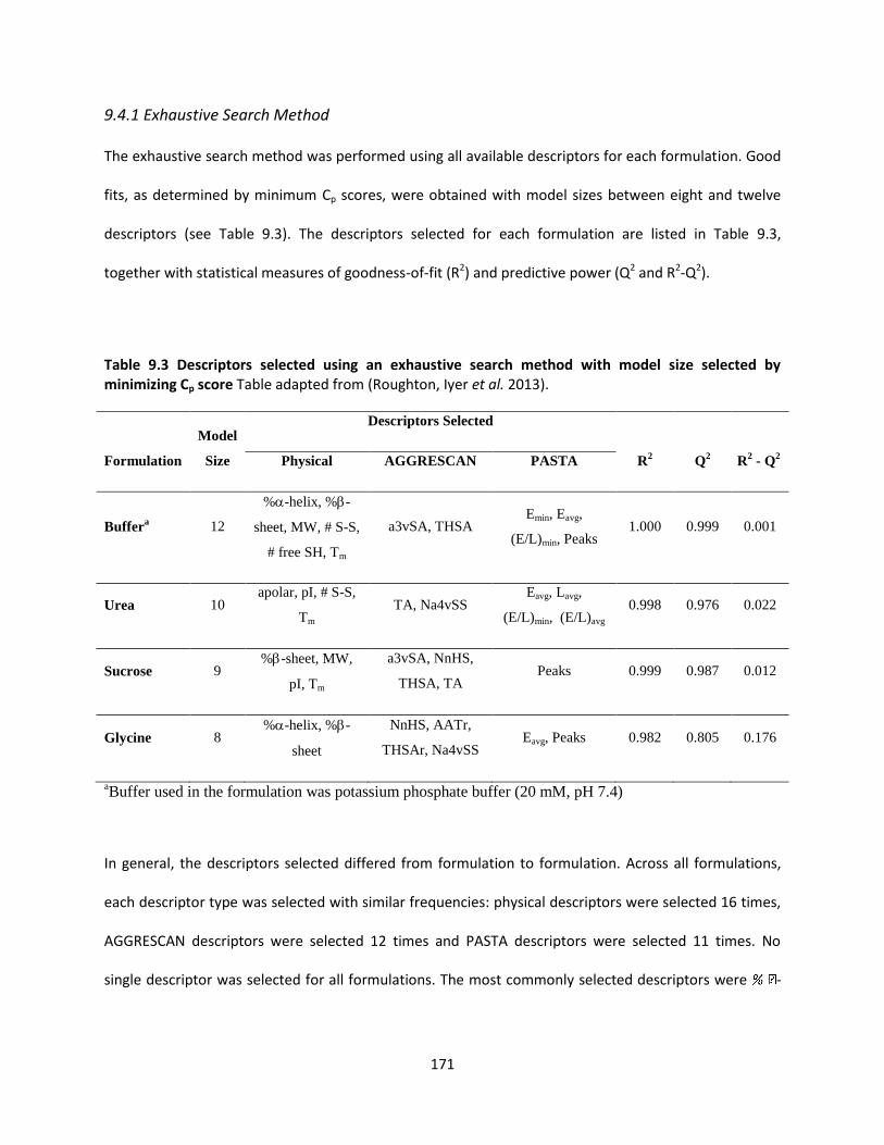
171
9.4.1 Exhaustive Search Method
The exhaustive search method was performed using all available descriptors for each formulation. Good
fits, as determined by minimum Cp scores, were obtained with model sizes between eight and twelve
descriptors (see Table 9.3). The descriptors selected for each formulation are listed in Table 9.3,
together with statistical measures of goodness-of-fit (R2) and predictive power (Q2 and R2-Q2).
Table 9.3 Descriptors selected using an exhaustive search method with model size selected by minimizing Cp score Table adapted from (Roughton, Iyer et al. 2013).
Formulation
Model
Size
Descriptors Selected
R2 Q
2 R
2 - Q
2 Physical AGGRESCAN PASTA
Buffera 12
%-helix, %-
sheet, MW, # S-S,
# free SH, Tm
a3vSA, THSA Emin, Eavg,
(E/L)min, Peaks 1.000 0.999 0.001
Urea 10 apolar, pI, # S-S,
Tm TA, Na4vSS
Eavg, Lavg,
(E/L)min, (E/L)avg 0.998 0.976 0.022
Sucrose 9 %-sheet, MW,
pI, Tm
a3vSA, NnHS,
THSA, TA Peaks 0.999 0.987 0.012
Glycine 8 %-helix, %-
sheet
NnHS, AATr,
THSAr, Na4vSS Eavg, Peaks 0.982 0.805 0.176
aBuffer used in the formulation was potassium phosphate buffer (20 mM, pH 7.4)
In general, the descriptors selected differed from formulation to formulation. Across all formulations,
each descriptor type was selected with similar frequencies: physical descriptors were selected 16 times,
AGGRESCAN descriptors were selected 12 times and PASTA descriptors were selected 11 times. No
single descriptor was selected for all formulations. The most commonly selected descriptors were -
172
sheet, Tm, Eavg, and Peaks, which were all selected for three of the four formulations. At least one
descriptor of each type was selected for each formulation.
The correlations for all four formulations had (R2-Q2) < 0.20 and R2 values close to 1, indicating that they
provide a reasonable tool for predicting the percent retained monomeric protein after lyophilization
within each formulation type. The correlation for the buffer formulation had the best fit and best
predictive power, having the highest R2 and Q2 values and the lowest (R2-Q2) values. The correlation for
the glycine formulation provided the poorest fit and lowest Q2 value, and also provided the poorest
predictive power as indicated by the largest (R2-Q2) value. A summary of the regression for the four
formulations, together with values of the regression coefficients, is presented in Table 9.4.
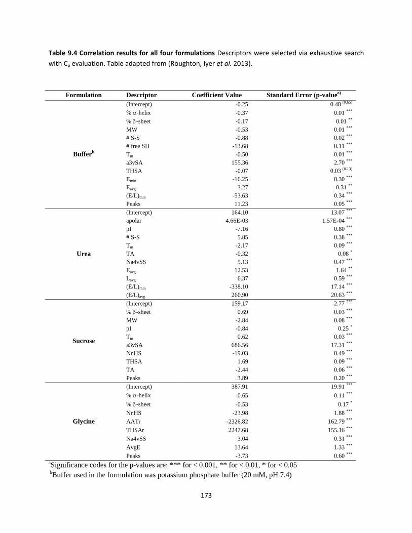
173
Table 9.4 Correlation results for all four formulations Descriptors were selected via exhaustive search
with Cp evaluation. Table adapted from (Roughton, Iyer et al. 2013).
Formulation Descriptor Coefficient Value Standard Error (p-valuea)
Bufferb
(Intercept) -0.25 0.48 (0.65)
% -helix -0.37 0.01 ***
% -sheet -0.17 0.01 **
MW -0.53 0.01 ***
# S-S -0.88 0.02 ***
# free SH -13.68 0.11 ***
Tm -0.50 0.01 ***
a3vSA 155.36 2.70 ***
THSA -0.07 0.03 (0.13)
Emin -16.25 0.30 ***
Eavg 3.27 0.31 **
(E/L)min -53.63 0.34 ***
Peaks 11.23 0.05 ***
Urea
(Intercept) 164.10 13.07 ***
apolar 4.66E-03 1.57E-04 ***
pI -7.16 0.80 ***
# S-S 5.85 0.38 ***
Tm -2.17 0.09 ***
TA -0.32 0.08 *
Na4vSS 5.13 0.47 ***
Eavg 12.53 1.64 **
Lavg 6.37 0.59 ***
(E/L)min -338.10 17.14 ***
(E/L)avg 260.90 20.63 ***
Sucrose
(Intercept) 159.17 2.77 ***
% -sheet 0.69 0.03 ***
MW -2.84 0.08 ***
pI -0.84 0.25 *
Tm 0.62 0.03 ***
a3vSA 686.56 17.31 ***
NnHS -19.03 0.49 ***
THSA 1.69 0.09 ***
TA -2.44 0.06 ***
Peaks 3.89 0.20 ***
Glycine
(Intercept) 387.91 19.91 ***
% -helix -0.65 0.11 ***
% -sheet -0.53 0.17 *
NnHS -23.98 1.88 ***
AATr -2326.82 162.79 ***
THSAr 2247.68 155.16 ***
Na4vSS 3.04 0.31 ***
AvgE 13.64 1.33 ***
Peaks -3.73 0.60 *** aSignificance codes for the p-values are: *** for < 0.001, ** for < 0.01, * for < 0.05
bBuffer used in the formulation was potassium phosphate buffer (20 mM, pH 7.4)

174
9.4.2 Forward Selection Method
Forward selection was also used to build correlations using all available descriptors. The computational
package used for forward selection used AIC for descriptor selection; however, AIC yields equivalent
models to Cp for linear correlations (Wasserman 2004), resulting in no discrepancy between descriptor
selection between the forward search and exhaustive search methods. Due to the nature of the
selection method, the final correlations differ in the number of descriptors selected (see Table 9.5).
Physical descriptors were selected most frequently with this method, accounting for 9 out of the 11
descriptors selected (see Table 9.5). Only physical descriptors were selected for urea and sucrose
formulations and four out of the five descriptors selected for the buffer formulation were physical
descriptors. The most commonly selected descriptor was pI, which was selected first for the buffer and
sucrose formulations and second for the urea formulation. The early selection of pI indicates that this
descriptor provides a superior fit to the experimental data for the buffer and sucrose formulations and a
very good fit for the urea formulation when compared to the other descriptors.
Table 9.5 Descriptors selected using a forward search method with AIC evaluation Numbering
indicates order in which descriptors were selected. No emphasis indicates physical descriptors and bold
text indicates AGGRESCAN descriptors. No PASTA descriptors were selected. Table adapted from
(Roughton, Iyer et al. 2013).
Formulation
Descriptors Selected Regression Performance
1 2 3 5 R2 Q
2 R
2 - Q
2
Buffera pI Tm %-sheet -helix THSA 0.74 0.16 0.58
Urea # free SH pI Tm - - 0.54 0.11 0.43
Sucrose pI %-sheet - - - 0.57 0.19 0.38
Glycine a3vSA - - - - 0.14 -0.28 0.42
aBuffer used in the formulation was potassium phosphate buffer (20 mM, pH 7.4)
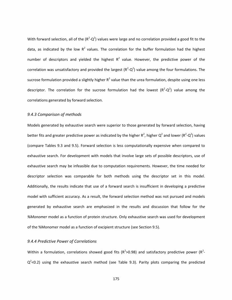
175
With forward selection, all of the (R2-Q2) values were large and no correlation provided a good fit to the
data, as indicated by the low R2 values. The correlation for the buffer formulation had the highest
number of descriptors and yielded the highest R2 value. However, the predictive power of the
correlation was unsatisfactory and provided the largest (R2-Q2) value among the four formulations. The
sucrose formulation provided a slightly higher R2 value than the urea formulation, despite using one less
descriptor. The correlation for the sucrose formulation had the lowest (R2-Q2) value among the
correlations generated by forward selection.
9.4.3 Comparison of methods
Models generated by exhaustive search were superior to those generated by forward selection, having
better fits and greater predictive power as indicated by the higher R2, higher Q2 and lower (R2-Q2) values
(compare Tables 9.3 and 9.5). Forward selection is less computationally expensive when compared to
exhaustive search. For development with models that involve large sets of possible descriptors, use of
exhaustive search may be infeasible due to computation requirements. However, the time needed for
descriptor selection was comparable for both methods using the descriptor set in this model.
Additionally, the results indicate that use of a forward search is insufficient in developing a predictive
model with sufficient accuracy. As a result, the forward selection method was not pursued and models
generated by exhaustive search are emphasized in the results and discussion that follow for the
%Monomer model as a function of protein structure. Only exhaustive search was used for development
of the %Monomer model as a function of excipient structure (see Section 9.5).
9.4.4 Predictive Power of Correlations
Within a formulation, correlations showed good fits (R2>0.98) and satisfactory predictive power (R2-
Q2<0.2) using the exhaustive search method (see Table 9.3). Parity plots comparing the predicted
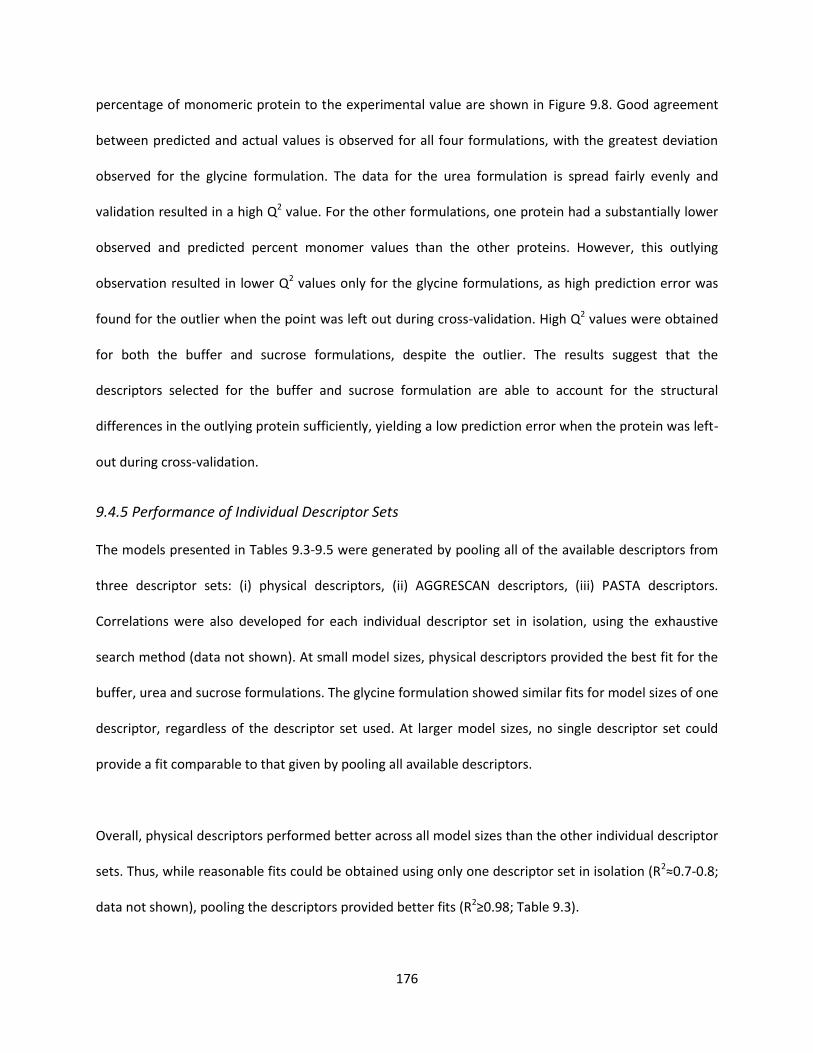
176
percentage of monomeric protein to the experimental value are shown in Figure 9.8. Good agreement
between predicted and actual values is observed for all four formulations, with the greatest deviation
observed for the glycine formulation. The data for the urea formulation is spread fairly evenly and
validation resulted in a high Q2 value. For the other formulations, one protein had a substantially lower
observed and predicted percent monomer values than the other proteins. However, this outlying
observation resulted in lower Q2 values only for the glycine formulations, as high prediction error was
found for the outlier when the point was left out during cross-validation. High Q2 values were obtained
for both the buffer and sucrose formulations, despite the outlier. The results suggest that the
descriptors selected for the buffer and sucrose formulation are able to account for the structural
differences in the outlying protein sufficiently, yielding a low prediction error when the protein was left-
out during cross-validation.
9.4.5 Performance of Individual Descriptor Sets
The models presented in Tables 9.3-9.5 were generated by pooling all of the available descriptors from
three descriptor sets: (i) physical descriptors, (ii) AGGRESCAN descriptors, (iii) PASTA descriptors.
Correlations were also developed for each individual descriptor set in isolation, using the exhaustive
search method (data not shown). At small model sizes, physical descriptors provided the best fit for the
buffer, urea and sucrose formulations. The glycine formulation showed similar fits for model sizes of one
descriptor, regardless of the descriptor set used. At larger model sizes, no single descriptor set could
provide a fit comparable to that given by pooling all available descriptors.
Overall, physical descriptors performed better across all model sizes than the other individual descriptor
sets. Thus, while reasonable fits could be obtained using only one descriptor set in isolation (R2≈0.7-0.8;
data not shown), pooling the descriptors provided better fits (R2≥0.9 Table 9.3).

177
(A) (B)
(C) (D)
Figure 9.8 Parity plots of experimental percent monomeric protein values (%Monomer) from SEC versus predicted %Monomer values Correlations were developed for (A) urea, (B) buffer (potassium
phosphate 20 mM, pH 7.4), (C) sucrose, and (D) glycine formulations. Figure adapted from (Roughton,
Iyer et al. 2013).
-20
0
20
40
60
80
100
120
140
-20 0 20 40 60 80 100 120 140
Pre
dic
ted
% M
on
om
er
Experimental % Monomer
20
40
60
80
100
120
20 40 60 80 100 120
Pre
dic
ted
% M
on
om
er
Experimental % Monomer
20
40
60
80
100
120
20 40 60 80 100 120
Pre
dic
ted
% M
on
om
er
Experimental % Monomer
40
60
80
100
120
140
40 60 80 100 120 140
Pre
dic
ted
% M
on
om
er
Experimental % Monomer
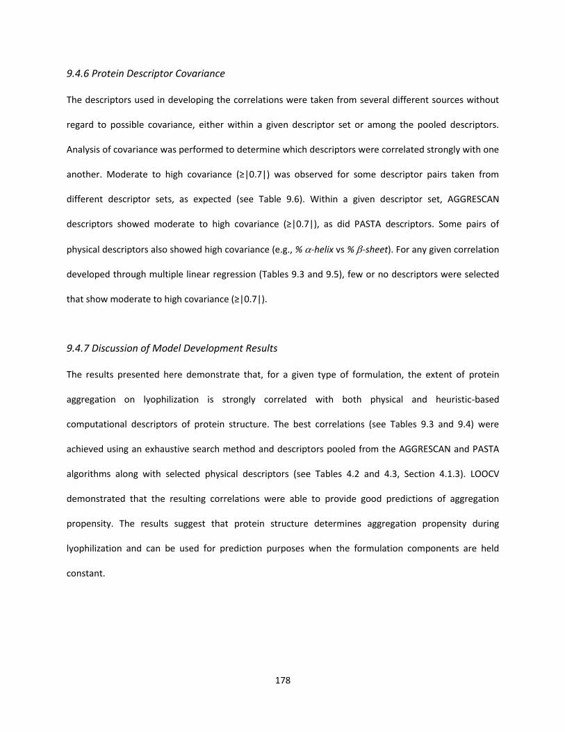
178
9.4.6 Protein Descriptor Covariance
The descriptors used in developing the correlations were taken from several different sources without
regard to possible covariance, either within a given descriptor set or among the pooled descriptors.
Analysis of covariance was performed to determine which descriptors were correlated strongly with one
another. Moderate to high covariance (≥|0.7|) was observed for some descriptor pairs ta en from
different descriptor sets, as expected (see Table 9.6). Within a given descriptor set, AGGRESCAN
descriptors showed moderate to high covariance (≥|0.7|), as did PASTA descriptors. Some pairs of
physical descriptors also showed high covariance (e.g., % -helix vs % -sheet). For any given correlation
developed through multiple linear regression (Tables 9.3 and 9.5), few or no descriptors were selected
that show moderate to high covariance (≥|0.7|).
9.4.7 Discussion of Model Development Results
The results presented here demonstrate that, for a given type of formulation, the extent of protein
aggregation on lyophilization is strongly correlated with both physical and heuristic-based
computational descriptors of protein structure. The best correlations (see Tables 9.3 and 9.4) were
achieved using an exhaustive search method and descriptors pooled from the AGGRESCAN and PASTA
algorithms along with selected physical descriptors (see Tables 4.2 and 4.3, Section 4.1.3). LOOCV
demonstrated that the resulting correlations were able to provide good predictions of aggregation
propensity. The results suggest that protein structure determines aggregation propensity during
lyophilization and can be used for prediction purposes when the formulation components are held
constant.

179
Table 9.6 Summary of covariance analysis Variable pairs with high degrees of covariance are given.
Note that |Covariance (X,Y)| = |Covariance(Y,X)|. Table adapted from (Roughton, Iyer et al. 2013).
| ( )| | ( )| | ( )|
(apolar, MW)
(Lmax, (E/L)avg)
((E/L)min, (E/L)avg)
(a3vSA, Emin)
(a3vSA, Eavg)
(MW, AAT)
(AAT, Emin)
(AAT, Eavg)
(THSA, Emin)
(THSA, Eavg)
(a3vSA, THSA)
(a3vSA, TA)
(a3vSA, AATr)
(TA, AATr)
(a3vSA, THSAr)
(NnHS, THSAr)
(Na4vSS, Emin)
(Na4vSS, Eavg)
(Na4vSS, THSA)
(Na4vSS, TA)
(Na4vSS, AATr)
(Na4vSS, THSAr)
(% -helix, % -sheet)
(apolar, # free SH)
(MW, nHS)
(AAT, nHS)
(THSA, nHS)
(Eavg, Emin)
(Lavg, Lmax)
(Na4vSS, a3vSA)
Independently, each of the heuristic-based algorithms provided considerably poorer correlations with
lower predictive power than those built from pooled set of descriptors. The descriptors from both the
AGGRESCAN and PASTA sets showed high covariance (see Table 9.6). As a result, the amount of
structural information captured by either method is limited despite the large number of descriptors
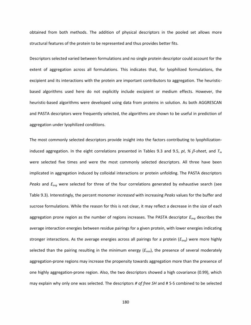
180
obtained from both methods. The addition of physical descriptors in the pooled set allows more
structural features of the protein to be represented and thus provides better fits.
Descriptors selected varied between formulations and no single protein descriptor could account for the
extent of aggregation across all formulations. This indicates that, for lyophilized formulations, the
excipient and its interactions with the protein are important contributors to aggregation. The heuristic-
based algorithms used here do not explicitly include excipient or medium effects. However, the
heuristic-based algorithms were developed using data from proteins in solution. As both AGGRESCAN
and PASTA descriptors were frequently selected, the algorithms are shown to be useful in prediction of
aggregation under lyophilized conditions.
The most commonly selected descriptors provide insight into the factors contributing to lyophilization-
induced aggregation. In the eight correlations presented in Tables 9.3 and 9.5, pI, % -sheet, and Tm
were selected five times and were the most commonly selected descriptors. All three have been
implicated in aggregation induced by colloidal interactions or protein unfolding. The PASTA descriptors
Peaks and Eavg were selected for three of the four correlations generated by exhaustive search (see
Table 9.3). Interestingly, the percent monomer increased with increasing Peaks values for the buffer and
sucrose formulations. While the reason for this is not clear, it may reflect a decrease in the size of each
aggregation prone region as the number of regions increases. The PASTA descriptor Eavg describes the
average interaction energies between residue pairings for a given protein, with lower energies indicating
stronger interactions. As the average energies across all pairings for a protein (Eavg) were more highly
selected than the pairing resulting in the minimum energy (Emin), the presence of several moderately
aggregation-prone regions may increase the propensity towards aggregation more than the presence of
one highly aggregation-prone region. Also, the two descriptors showed a high covariance (0.99), which
may explain why only one was selected. The descriptors # of free SH and # S-S combined to be selected

181
in four of the eight correlations. The frequent selection of thiol/disulfide related descriptors is not
surprising, since free thiol groups are reactive and can lead to the formation of disulfide-linked covalent
aggregates. SDS-PAGE results confirmed that reducible aggregates were observed for proteins
containing four or more free thiol groups (Table F.1, Appendix F).
Examination of the descriptors that were not selected is also instructive. Apolar surface area (apolar)
and fractional apolar surface area (fapolar) were not highly selected. The lack of selection of apolar
suggests that aggregation during lyophilization is not strongly correlated to total apolar surface area.
Furthermore, larger percentages of apolar surface area do not appear to affect aggregation as fapolar was
not chosen for any of the correlations.
The predictive ability of the correlations is expected to be greatest for proteins whose properties fall
within the structural space defined by the 15 proteins studied here. Perhaps more importantly, the
correlations are limited in that the effects of excipients on aggregation are not included quantitatively,
since the number of excipients tested was small.
9.5 POST-LYOPHILIZATION PROTEIN LOSS MODELS: AS A FUNCTION OF EXCIPIENT STRUCTURE
Models were developed to describe %Monomer as a function of excipient structure. During model
development, several techniques were introduced to further gain insight into the models developed.
Principle component analysis (PCA) was used to investigate the descriptor space. The impact of using
chiral connectivity indices versus simple connectivity indices was determined. Finally, K-fold cross-
validation was used in addition to LOOCV to further probe the predictive power of the models presented
here.

182
9.5.1 Principal Component Analysis and Descriptor Comparison
Both simple connectivity indices and chiral connectivity indices up to the fifth order were considered for
use as descriptors for development of the protein-by-protein linear models. PCA was performed using
the chiral connectivity indices to visualize the descriptor space for the molecules considered (see Figure
9.9). Two principal components were sufficient to account for 99% of the variance observed in the data
set, allowing a two dimensional representation of the descriptor space to be sufficient. PCA revealed
three main clusters of excipient structures roughly correlating with monosaccharides, disaccharides and
trisaccharides.
Figure 9.9 Principal component analysis of descriptor space for excipients used in study The “X”
marker represents N-acetyl-neuraminic acid. Filled in markers represent excipients used for all proteins
while un-filled markers represent excipients used only with BSA and RNAse A. Descriptors used to
construct the principal components are connectivity indices up to the fifth order with a chirality
correction factor of two.
Chirality connectivity indices were able to provide fits with good accuracy (R2 > 0.9) for -amylase,
ovalbumin and trypsin inhibitor. Simple connectivity indices were unable to provide fits with sufficient
-4
-2
0
2
4
6
8
10
12
-60 -50 -40 -30 -20 -10 0
Pri
nci
pal
Co
mp
on
en
t 2
Principal Component 1
Sugar Alcohols
Monosaccharides
Disaccharides
Trisaccharides
Amino Acids

183
accuracy. For BSA and RNAse A, neither class of descriptors was able to yield a model with acceptable
accuracy. Excipients derived from amino acids were considered for BSA and RNAse A formulations, but
were not considered for the other proteins. PCA results suggested that the amino acid based excipients
were structurally similar to the monosaccharides considered (see Figure 9.9). However, the molecular
descriptors used do not explicitly account for charge. Amino acids are either charged or zwitterionic at
the solution conditions used in the study. Separation of the data into two sets (a carbohydrate set and
amino acid set) provided correlations with increased accuracy when using chiral connectivity indices for
the carbohydrate data set and when using either type of connectivity indices for the amino acid set (see
Figure 9.10). Chiral connectivity indices were used for model development for all carbohydrate data
sets. As no molecule belonging to the amino acid class contains more than one chiral center and all
chiral centers are S-configuration, simple connectivity indices were used instead of chiral connectivity
indices for model development for all amino acid data sets.
Figure 9.10 Comparison of chiral and simple connectivity indices for BSA and RNAse carbohydrate models Each point represents the model with the maximum R2 for the given number of descriptors.
Each model building set contained 20 data points.
0
0.1
0.2
0.3
0.4
0.5
0.6
0.7
0.8
0.9
1
0 5 10 15 20
R2
Number of Descriptors
R²-BSA Chiral
R²-BSA Simple
R²-RNAse A Chiral
R²-RNAse A Simple
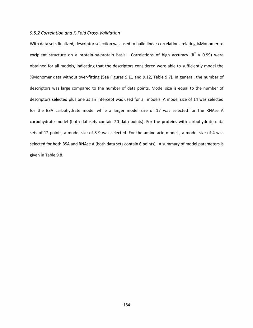
184
9.5.2 Correlation and K-Fold Cross-Validation
With data sets finalized, descriptor selection was used to build linear correlations relating %Monomer to
excipient structure on a protein-by-protein basis. Correlations of high accuracy (R2 ≈ 0.99) were
obtained for all models, indicating that the descriptors considered were able to sufficiently model the
%Monomer data without over-fitting (See Figures 9.11 and 9.12, Table 9.7). In general, the number of
descriptors was large compared to the number of data points. Model size is equal to the number of
descriptors selected plus one as an intercept was used for all models. A model size of 14 was selected
for the BSA carbohydrate model while a larger model size of 17 was selected for the RNAse A
carbohydrate model (both datasets contain 20 data points). For the proteins with carbohydrate data
sets of 12 points, a model size of 8-9 was selected. For the amino acid models, a model size of 4 was
selected for both BSA and RNAse A (both data sets contain 6 points). A summary of model parameters is
given in Table 9.8.
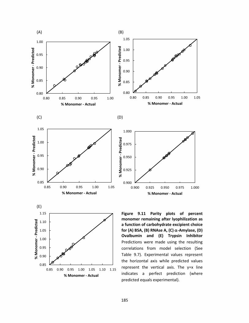
185
(A) (B)
(C) (D)
(E)
0.80
0.85
0.90
0.95
1.00
0.80 0.85 0.90 0.95 1.00
% M
on
om
er
- P
red
icte
d
% Monomer - Actual
0.80
0.85
0.90
0.95
1.00
1.05
0.80 0.85 0.90 0.95 1.00 1.05
% M
on
om
er
- P
red
icte
d
% Monomer - Actual
0.85
0.90
0.95
1.00
1.05
0.85 0.90 0.95 1.00 1.05
% M
on
om
er
- P
red
icte
d
% Monomer - Actual
0.900
0.925
0.950
0.975
1.000
0.900 0.925 0.950 0.975 1.000
% M
on
om
er
- P
red
icte
d
% Monomer - Actual
0.85
0.90
0.95
1.00
1.05
1.10
1.15
0.85 0.90 0.95 1.00 1.05 1.10 1.15
% M
on
om
er
- P
red
icte
d
% Monomer - Actual
Figure 9.11 Parity plots of percent monomer remaining after lyophilization as a function of carbohydrate excipient choice
for (A) BSA, (B) RNAse A, (C) -Amylase, (D) Ovalbumin and (E) Trypsin Inhibitor
Predictions were made using the resulting
correlations from model selection (See
Table 9.7). Experimental values represent
the horizontal axis while predicted values
represent the vertical axis. The y=x line
indicates a perfect prediction (where
predicted equals experimental).

186
(A) (B)
Figure 9.12 Parity plots of percent monomer remaining after lyophilization as a function of amino acid excipient choice for (A) BSA and (B) RNAse A Predictions were made using the resulting correlations
from model selection (See Table 9.7). Experimental values represent the horizontal axis while predicted
values represent the vertical axis. The y=x line indicates a perfect prediction (where predicted equals
experimental).
K-fold cross-validation was performed to test the predictive power of the models. As more data is left
out in each fold, the number of folds (K) generated from the data set decreases and the resulting Q2 is
expected to decrease. As a rule, a Q2 ≥ 0. is desired (Golbraikh, Shen et al. 2003). Folds were increased
in size and Q2 was evaluated until a value was obtained below 0.6 (see Table 9.7). The size of the fold
obtained at the lowest K value where Q2 ≥ 0. gives an indication of how much data can be left-out
while retaining reliable prediction accuracy. Thus the results give an estimation of the minimum number
of points in a given set of molecules that are required to be known experimentally. Ideally, the number
would be low so that a small number of data points are sufficient to build a widely applicable predictive
model.
For the BSA carbohydrate model, the minimum acceptable number of folds was K=5 (corresponding to a
fold size of 4 or 20% of the data). The RNAse A model however showed an unacceptable Q2 value for the
0.88
0.89
0.90
0.91
0.92
0.93
0.94
0.88 0.89 0.90 0.91 0.92 0.93 0.94
% M
on
om
er
- P
red
icte
d
% Monomer - Actual
0.94
0.95
0.96
0.97
0.98
0.99
1.00
0.94 0.95 0.96 0.97 0.98 0.99 1.00
% M
on
om
er
- P
red
icte
d
% Monomer - Actual
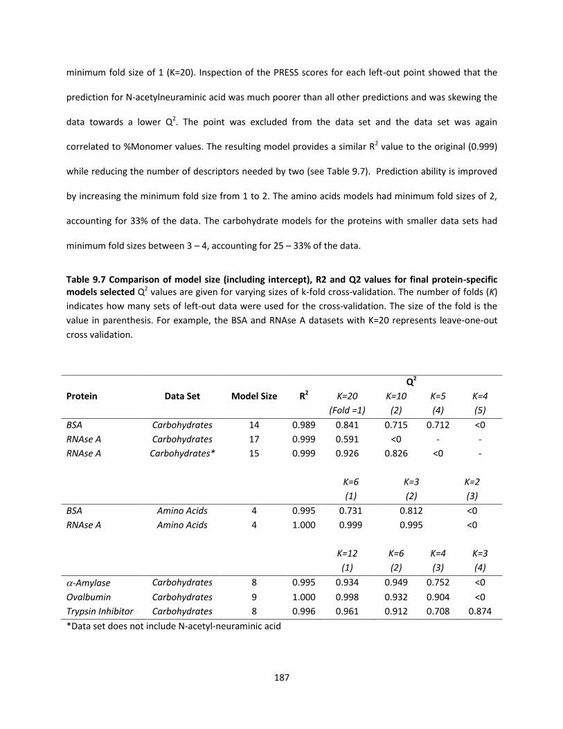
187
minimum fold size of 1 (K=20). Inspection of the PRESS scores for each left-out point showed that the
prediction for N-acetylneuraminic acid was much poorer than all other predictions and was skewing the
data towards a lower Q2. The point was excluded from the data set and the data set was again
correlated to %Monomer values. The resulting model provides a similar R2 value to the original (0.999)
while reducing the number of descriptors needed by two (see Table 9.7). Prediction ability is improved
by increasing the minimum fold size from 1 to 2. The amino acids models had minimum fold sizes of 2,
accounting for 33% of the data. The carbohydrate models for the proteins with smaller data sets had
minimum fold sizes between 3 – 4, accounting for 25 – 33% of the data.
Table 9.7 Comparison of model size (including intercept), R2 and Q2 values for final protein-specific models selected Q2 values are given for varying sizes of k-fold cross-validation. The number of folds (K)
indicates how many sets of left-out data were used for the cross-validation. The size of the fold is the
value in parenthesis. For example, the BSA and RNAse A datasets with K=20 represents leave-one-out
cross validation.
Q2
Protein Data Set Model Size R2 K=20
(Fold =1)
K=10
(2)
K=5
(4)
K=4
(5)
BSA Carbohydrates 14 0.989 0.841 0.715 0.712 <0
RNAse A Carbohydrates 17 0.999 0.591 <0 - -
RNAse A Carbohydrates* 15 0.999 0.926 0.826 <0 -
K=6
(1)
K=3
(2)
K=2
(3)
BSA Amino Acids 4 0.995 0.731 0.812 <0
RNAse A Amino Acids 4 1.000 0.999 0.995 <0
K=12
(1)
K=6
(2)
K=4
(3)
K=3
(4)
-Amylase Carbohydrates 8 0.995 0.934 0.949 0.752 <0
Ovalbumin Carbohydrates 9 1.000 0.998 0.932 0.904 <0
Trypsin Inhibitor Carbohydrates 8 0.996 0.961 0.912 0.708 0.874
*Data set does not include N-acetyl-neuraminic acid

188
9.5.3 Discussion of Model Development Results
Development of the protein-by-protein models illustrates that protein stability following lyophilization is
strongly correlated to excipient choice. The need to separate amino acids from carbohydrates indicates
that while structurally similar to monosaccharaides on the basis of molecular connectivity (see Figure
9.9), the structural features of the two molecular classes act in different ways to stabilize the protein.
Additionally, cross-validation revealed that N-acetyl neuraminic acid was the carbohydrate molecule
with the largest prediction errors. Structural comparisons show that N-acetyl neuraminic acid is similar
to disaccharides (see Figure 9.9). The descriptors used do not account for charge, which is present in
amino acids and N-acetylneuraminic acid at the solution conditions considered. Accounting for charge
may offer a means to unify the carbohydrate and amino acid models into one model and improve
prediction for carbohydrate molecules containing charges. The improvement of the carbohydrate
models through use of chiral connectivity indices (see Figure 9.10) indicates that the three-dimensional
conformation is an important feature of the excipient in the stabilization of the protein.
The cross-validation analysis suggests that the maximum amount of data acceptable to leave out was
33%, which suggests the need to take at least 2/3 of the data experimentally in order to build a reliable
and predictive model. However, the analysis does not suggest a hard and fast rule when developing
similar models. Indeed, these numbers could likely be improved by rationally designing the test and
training set (Golbraikh, Shen et al. 2003) and/or focusing the data set to a more restrictive molecular
class, such as monosaccharides rather than carbohydrates.
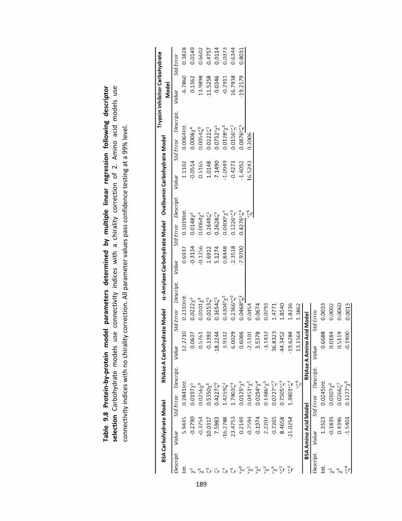
189
Tab
le
9.8
P
rote
in-b
y-p
rote
in
mo
de
l p
aram
ete
rs
de
term
ine
d
by
mu
ltip
le
line
ar
regr
essi
on
fo
llow
ing
des
crip
tor
sele
ctio
n
Car
bo
hyd
rate
mo
del
s u
se
con
ne
ctiv
ity
ind
ices
w
ith
a
chir
alit
y co
rrec
tio
n
of
2.
Am
ino
ac
id
mo
del
s u
se
con
nec
tivi
ty in
dic
es w
ith
no
ch
iral
ity
corr
ecti
on
. All
par
amet
er
valu
es p
ass
con
fid
ence
tes
tin
g at
a 9
9%
leve
l.

190
9.6 POST-LYOPHILIZATION PROTEIN LOSS MODELS: AS A FUNCTION OF BOTH PROTEIN AND
EXCIPIENT STRUCTURE
Chiral connectivity indices and all discussed protein descriptors were used as potential descriptors for
the universal model. Only data for formulations containing carbohydrate excipients were considered,
resulting in a data set of 73 %Monomer values. The resulting model required a non-linear form, which
required differences in model development as compared to the linear models described previously.
9.6.1 Non-Linear Model Development
Attempts to build a linear model of sufficient correlative quality were unsuccessful (results not shown).
Non-linear models were considered to better correlate the descriptors to the %Monomer values.
Several functional forms were considered, with the best form given by Equation 9.5.
(∑ ) (∑ )
(Equation 9.5)
where represents excipient descriptors, represents protein descriptors, and a, b, and c are
adjustable parameters. All descriptors considered were used initially for model development, with 24
descriptors accounting for excipient structure and 25 descriptors accounting for protein structure. Given
the parameters determined for each descriptor, a parameter sensitivity analysis was performed to
identify the parameters that had no impact on the model prediction. In total 13 descriptors were
identified as having no impact on the model prediction, with two descriptors accounting for excipient
structure and 11 descriptors accounting for protein structure (see Table 9.9). The descriptors were
removed and the model parameters were again determined for the scaling constant (c) and the
remaining 20 excipient and 6 protein descriptors. After one round of descriptor reduction, the model
%AAD = 2.58% and reduced chi-squared = 3.23 (see Table 9.10 and Figure 9.13).
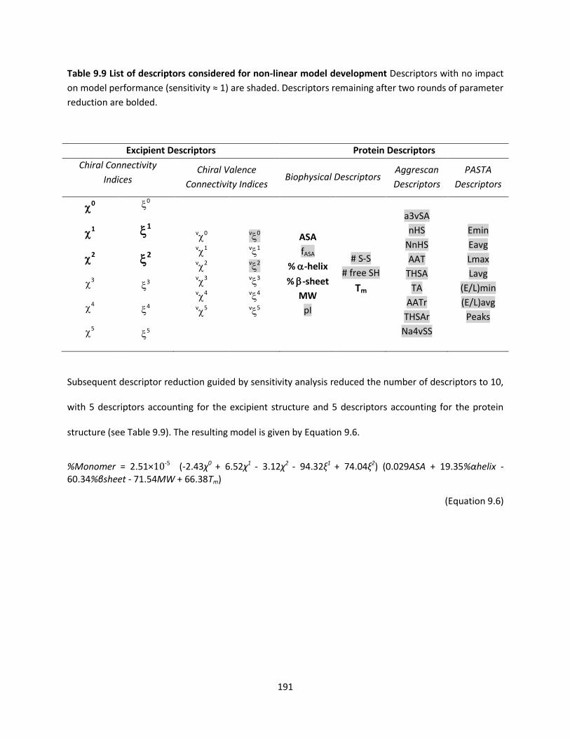
191
Table 9.9 List of descriptors considered for non-linear model development Descriptors with no impact
on model performance (sensitivity ≈ 1) are shaded. Descriptors remaining after two rounds of parameter
reduction are bolded.
Excipient Descriptors Protein Descriptors
Chiral Connectivity
Indices Chiral Valence
Connectivity Indices Biophysical Descriptors
Aggrescan
Descriptors
PASTA
Descriptors
0
1
2
3
4
5
0
1
2
3
4
5
v
0 v
1
v
2
v
3
v
4
v
5
v
0 v
1
v
2
v
3
v
4
v
5
ASA
fASA
% -helix
% -sheet
MW
pI
# S-S
# free SH
Tm
a3vSA
nHS
NnHS
AAT
THSA
TA
AATr
THSAr
Na4vSS
Emin
Eavg
Lmax
Lavg
(E/L)min
(E/L)avg
Peaks
Subsequent descriptor reduction guided by sensitivity analysis reduced the number of descriptors to 10,
with 5 descriptors accounting for the excipient structure and 5 descriptors accounting for the protein
structure (see Table 9.9). The resulting model is given by Equation 9.6.
%Monomer = 2.51×10⁻⁵ (-2.43χ0 + 6.52χ1 - 3.12χ2 - 94.32ξ1 + 74.04ξ2) (0.029ASA + 19.35%αhelix - 60.34%βsheet - 71.54MW + 66.38Tm)
(Equation 9.6)
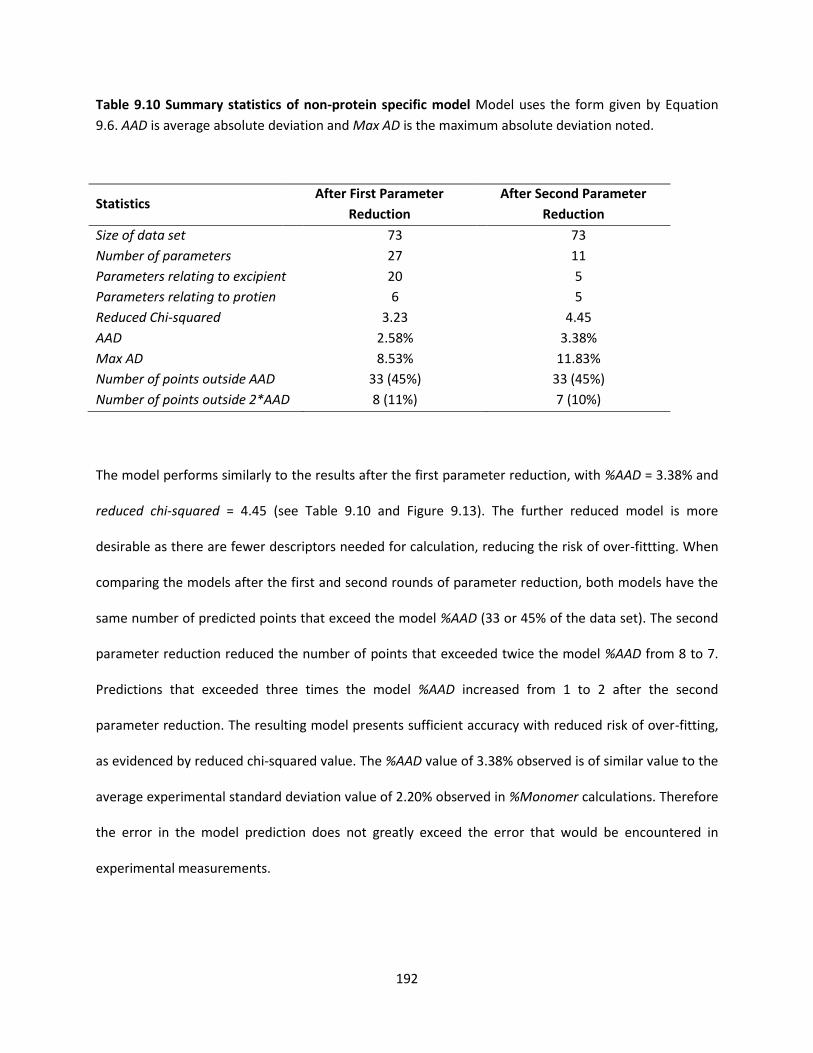
192
Table 9.10 Summary statistics of non-protein specific model Model uses the form given by Equation
9.6. AAD is average absolute deviation and Max AD is the maximum absolute deviation noted.
Statistics After First Parameter
Reduction
After Second Parameter
Reduction
Size of data set 73 73
Number of parameters 27 11
Parameters relating to excipient 20 5
Parameters relating to protien 6 5
Reduced Chi-squared 3.23 4.45
AAD 2.58% 3.38%
Max AD 8.53% 11.83%
Number of points outside AAD 33 (45%) 33 (45%)
Number of points outside 2*AAD 8 (11%) 7 (10%)
The model performs similarly to the results after the first parameter reduction, with %AAD = 3.38% and
reduced chi-squared = 4.45 (see Table 9.10 and Figure 9.13). The further reduced model is more
desirable as there are fewer descriptors needed for calculation, reducing the risk of over-fittting. When
comparing the models after the first and second rounds of parameter reduction, both models have the
same number of predicted points that exceed the model %AAD (33 or 45% of the data set). The second
parameter reduction reduced the number of points that exceeded twice the model %AAD from 8 to 7.
Predictions that exceeded three times the model %AAD increased from 1 to 2 after the second
parameter reduction. The resulting model presents sufficient accuracy with reduced risk of over-fitting,
as evidenced by reduced chi-squared value. The %AAD value of 3.38% observed is of similar value to the
average experimental standard deviation value of 2.20% observed in %Monomer calculations. Therefore
the error in the model prediction does not greatly exceed the error that would be encountered in
experimental measurements.

193
(A) (B)
Figure 9.13 Parity plots of percent monomer remaining after lyophilization as a function of both protein and excipient structure Predictions were made using results for non-linear model
development. (A) represents model after first parameter reduction and (B) represents model after
second parameter reduction. Experimental values represent the horizontal axis while predicted values
represent the vertical axis. The y=x line indicates a perfect prediction (where predicted equals
experimental).
9.6.2 Discussion of Results from Model Development
Several functional forms for a model describing protein stability following lyophilization as a function of
excipient choice and protein choice were considered. The final form used is given by Equation 9.6, which
was motivated by the enthalpic contribution of the Flory-Huggins model, given by Equation 9.7. The
Flory-Huggins model has been used previously to describe protein-sugar interactions in lyophilized solids
(Katayama, Carpenter et al. 2009; Wang, Tchessalov et al. 2009). Equation 9.6 emulates the Flory-
Huggins interaction parameter (12) through the multiplication of excipient structural descriptors and
protein structural descriptors. The success of the Flory-Huggins functional form of the universal model
suggests that direct protein-excipient interactions may play a significant role in stabilization of the
protein during lyophilization for the formulations considered.
(Equation 9.7)
0.75
0.80
0.85
0.90
0.95
1.00
1.05
1.10
0.75 0.80 0.85 0.90 0.95 1.00 1.05 1.10
% M
on
om
er -
Pre
dic
ted
% Monomer - Actual
0.75
0.80
0.85
0.90
0.95
1.00
1.05
1.10
0.75 0.80 0.85 0.90 0.95 1.00 1.05 1.10
% M
on
om
er
- P
red
icte
d
% Monomer - Actual
194
Parameter sensitivity analysis revealed that all of the descriptors obtained or derived from aggregation
prediction methods had no significant impact on the model prediction (see Table 9.9). The results
suggest that AGGRESCAN and PASTA may not be applicable to aggregation induced by the lyophilization
process or at least are not the strongest predictors of aggregation in lyophilized systems. Both the
number of disulfide bridges and the number of free thiols had sensitivity values near unity, indicating
that intermolecular disulfide bond formation was not a primary cause of aggregation for the proteins
considered. The SDS-PAGE results support this conclusion as only ovalbumin showed reduction of
aggregate formation under reducing conditions (see Table F.3, Appendix F). The isoelectric point had a
sensitivity value of one, suggesting that charge-based associations were not driving forces for
aggregation in the proteins considered. Both %-helix and %-sheet were descriptors that were
retained in the final model, indicating that secondary structure was an important factor in protein
stability following lyophilization. The amount of -helix content increased protein stability while the
amount of -sheet content reduced protein stability. All excipient descriptors retained in the final model
were chiral connectivity indices of second order or less, suggesting that the short range connectivity
(bond paths of 2, bonds, and atoms present) was the most important excipient structural feature in
regards to protein stability.
The model presented provides predictions for protein stability following lyophilization as a function of
excipient choice and protein choice. Limitations on the model exist due to the data set used for
correlation. Only carbohydrates were considered, so extension to other classes of excipients is not
expected to provide accurate predictions. Additionally, predictions for proteins with structural features
that do not lie within the range of the proteins considered are not expected to be accurate. The success
of the model illustrates that such a model development procedure can be applied to other classes of
proteins and/or excipients for determination of predictive models for a given data set.
195
9.7 STOCHASTIC OPTIMIZATION TUNING RESULTS
Tuning of both a tabu search and genetic algorithm was performed to determine their suitability for
CAMD applications. For fair comparison, both methods used the same molecular representation. For
each parameter considered, 100 runs were performed for varying parameter values while all other
parameters were kept constant. Average value of the objective function, average time to solution,
percentage of runs that matched the target property (hit%) and percentage of runs that were within 5%
of the target property (close%) were the four measures used to guide tuning. Tuning was performed
through VBA on a PC with Windows 7 32-bit OS, Intel Core i5-2400 CPU @ 3.10 GHz, and 4.00 GB RAM.
Results for each stochastic optimization method follow.
9.7.1 Tabu search tuning results
For tabu search, four parameters were considered for tuning: the maximum number of non-improving
iterations, the maximum number of neighbors evaluated per iteration, the size of tabu list and the value
of tabu criterion (see Section 5.4 for more information on parameters). For each parameter value used
in tuning, 100 trials were conducted. Figures 9.14-9.17 display the tuning results for each of the
parameters considered.
The parameter with the most influence on objective function value and percentage of correct or nearly
correct solutions was the maximum number of non-improving iterations (see Figure 9.14). The result is
intuitive, as the longer the search is allowed to be performed the more likely that a very good result will
be found. As the maximum number of non-improving iterations is increased, the time to solution
increases linearly (R2 = 0.99, Figure 9.14). Consequently, a trade-off exists between solution quality and
solution efficiency. From tuning, a value of 100 maximum non-improving iterations was chosen as longer
searches had minimal effects on solution quality while greatly extending time to solution.
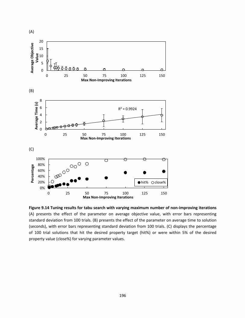
196
(A)
(B)
(C)
Figure 9.14 Tuning results for tabu search with varying maximum number of non-improving iterations
(A) presents the effect of the parameter on average objective value, with error bars representing
standard deviation from 100 trials. (B) presents the effect of the parameter on average time to solution
(seconds), with error bars representing standard deviation from 100 trials. (C) displays the percentage
of 100 trial solutions that hit the desired property target (hit%) or were within 5% of the desired
property value (close%) for varying parameter values.
0
5
10
15
20
0 25 50 75 100 125 150
Ave
rage
Ob
ject
ive
V
alu
e
Max Non-Improving Iterations
R² = 0.9924
0
2
4
6
8
0 25 50 75 100 125 150
Ave
rage
Tim
e (
s)
Max Non-Improving Iterations
0%
20%
40%
60%
80%
100%
0 25 50 75 100 125 150
Pe
rce
nta
ge
Max Non-Improving Iterations
hit% close%

197
(A)
(B)
(C)
Figure 9.15 Tuning results for tabu search with varying maximum number of neighbors considered at each iteration (A) presents the effect of the parameter on average objective value, with error bars
representing standard deviation from 100 trials. (B) presents the effect of the parameter on average
time to solution (seconds), with error bars representing standard deviation from 100 trials. (C) displays
the percentage of 100 trial solutions that hit the desired property target (hit%) or were within 5% of the
desired property value (close%) for varying parameter values.
0
2
4
6
0 1 2 3 4 5 6
Ave
rage
Ob
ject
ive
V
alu
e
Max Number of Neighbors Evaluated
R² = 0.9851
0
0.5
1
1.5
0 1 2 3 4 5 6
Ave
rage
Tim
e (
s)
Max Number of Neighbors Evaluated
0%
20%
40%
60%
80%
100%
0 1 2 3 4 5 6
Pe
rce
nta
ge
Max Number of Neighbors Evaluated
hit% close%
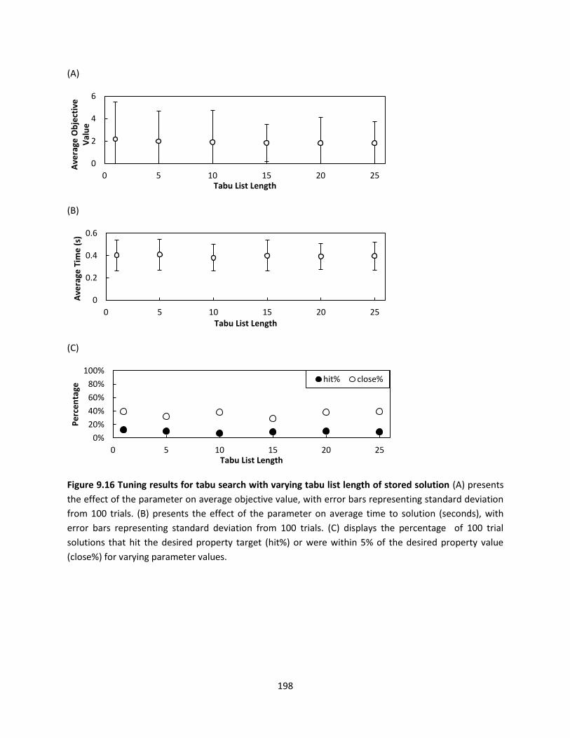
198
(A)
(B)
(C)
Figure 9.16 Tuning results for tabu search with varying tabu list length of stored solution (A) presents
the effect of the parameter on average objective value, with error bars representing standard deviation
from 100 trials. (B) presents the effect of the parameter on average time to solution (seconds), with
error bars representing standard deviation from 100 trials. (C) displays the percentage of 100 trial
solutions that hit the desired property target (hit%) or were within 5% of the desired property value
(close%) for varying parameter values.
0
2
4
6
0 5 10 15 20 25
Ave
rage
Ob
ject
ive
V
alu
e
Tabu List Length
0
0.2
0.4
0.6
0 5 10 15 20 25
Ave
rage
Tim
e (
s)
Tabu List Length
0%
20%
40%
60%
80%
100%
0 5 10 15 20 25
Pe
rce
nta
ge
Tabu List Length
hit% close%

199
(A)
(B)
(C)
Figure 9.17 Tuning results for tabu search with varying tabu criteria (A) presents the effect of the
parameter on average objective value, with error bars representing standard deviation from 100 trials.
(B) presents the effect of the parameter on average time to solution (seconds), with error bars
representing standard deviation from 100 trials. (C) displays the percentage of 100 trial solutions that
hit the desired property target (hit%) or were within 5% of the desired property value (close%) for
varying parameter values.
0
2
4
6
8
0 0.1 0.2 0.3 0.4 0.5 0.6 0.7 0.8 0.9 1
Ave
rage
Ob
ject
ive
V
alu
e
Tabu Criterion (D0)
R² = 0.8648
0
0.2
0.4
0.6
0.8
0 0.1 0.2 0.3 0.4 0.5 0.6 0.7 0.8 0.9 1
Ave
rage
Tim
e (
s)
Tabu Criterion (D0)
0%
20%
40%
60%
80%
100%
0 0.1 0.2 0.3 0.4 0.5 0.6 0.7 0.8 0.9 1
Pe
rce
nta
ge
Tabu Criterion (D0)
hit% close%

200
Increasing the maximum number of neighbors evaluated at each iteration and the tabu criterion also
lead to linear increases in time to solution (see Figure 9.15b and 9.17b). The time effect from increasing
the number of neighbors considered follows logically as more time is needed for evaluation and tabu
checks. The effect of increasing the tabu criterion is caused by placing too much restriction on the
search. As the tabu criterion becomes larger, it is more likely that a neighboring solution will be deemed
tabu. If too many solutions are declared tabu, the search will require more global moves and become
more time-consuming. The maximum number of neighbors was chosen to be four, as a discernible
increase in correct or nearly correct solutions is noted as the parameter changes from three to four (see
Figure 9.15c). The variability in average objective function value also noticeably decreases as the
maximum number of neighbors increase from three to four (see Figure 9.15a). Past four neighbors
considered, no benefit is gained in solution quality. Tabu criterion had no distinguishable effect on
solution quality and the base value of 0.5 was retained. The length of the tabu list had minimal effect on
solution quality and no effect on time to solution. The length of the tabu list was set at 15 as that
parameter value showed reduced variability in average objective function value (see Figure 9.16).
9.7.2 Genetic Algorithm Tuning Results
For the genetic algorithm, three parameters were considered for tuning: the maximum number of
generations, the size of population in each generation and the maximum probability that a member of
the population will be chosen as a parent (see Section 5.4 for more information on parameters). For
each parameter value investigate, 100 trials were performed. Figures 9.18-9.20 display the tuning
results for each of the parameters considered.
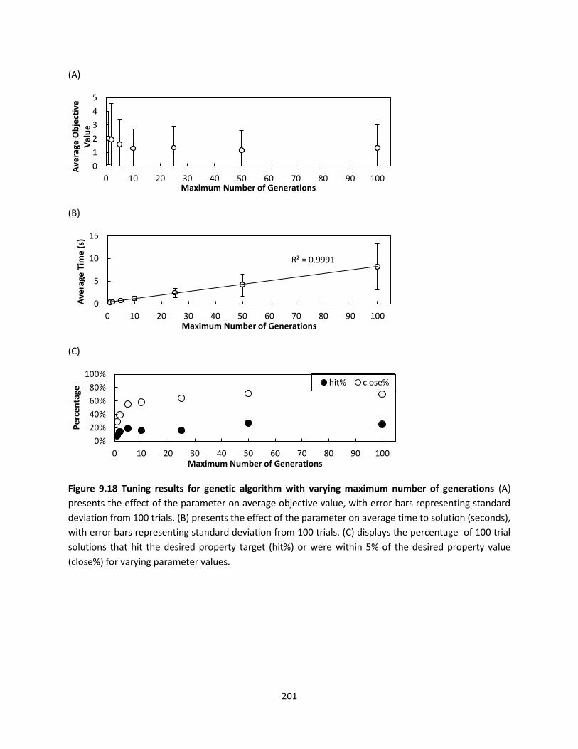
201
(A)
(B)
(C)
Figure 9.18 Tuning results for genetic algorithm with varying maximum number of generations (A)
presents the effect of the parameter on average objective value, with error bars representing standard
deviation from 100 trials. (B) presents the effect of the parameter on average time to solution (seconds),
with error bars representing standard deviation from 100 trials. (C) displays the percentage of 100 trial
solutions that hit the desired property target (hit%) or were within 5% of the desired property value
(close%) for varying parameter values.
0
1
2
3
4
5
0 10 20 30 40 50 60 70 80 90 100
Ave
rage
Ob
ject
ive
V
alu
e
Maximum Number of Generations
R² = 0.9991
0
5
10
15
0 10 20 30 40 50 60 70 80 90 100
Ave
rage
Tim
e (
s)
Maximum Number of Generations
0%
20%
40%
60%
80%
100%
0 10 20 30 40 50 60 70 80 90 100
Pe
rce
nta
ge
Maximum Number of Generations
hit% close%

202
(A)
(B)
(C)
Figure 9.19 Tuning results for genetic algorithm with population size per generation (A) presents the
effect of the parameter on average objective value, with error bars representing standard deviation
from 100 trials. (B) presents the effect of the parameter on average time to solution (seconds), with
error bars representing standard deviation from 100 trials. (C) displays the percentage of 100 trial
solutions that hit the desired property target (hit%) or were within 5% of the desired property value
(close%) for varying parameter values.
0
5
10
15
20
25
0 10 20 30 40 50
Ave
rage
Ob
ject
ive
V
alu
e
Population Size
R² = 0.993
0
2
4
6
8
0 10 20 30 40 50
Ave
rage
Tim
e (
s)
Population Size
0%
20%
40%
60%
80%
100%
0 10 20 30 40 50
Pe
rce
nta
ge
Population Size
hit% close%
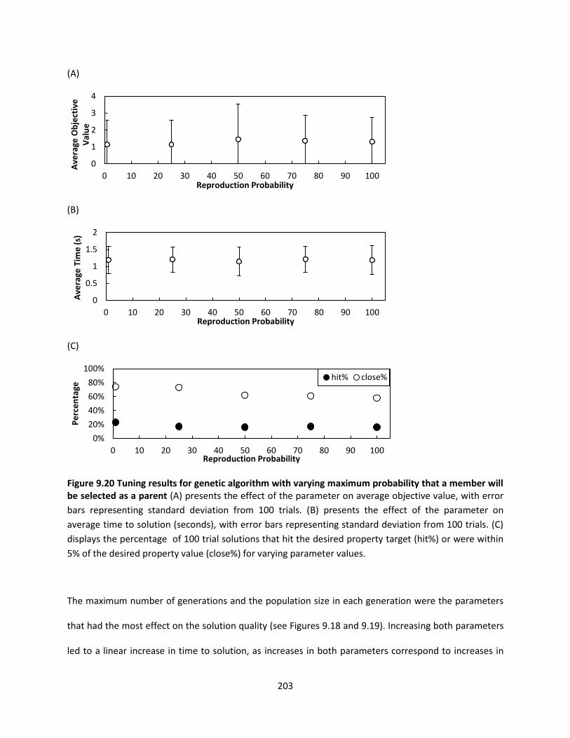
203
(A)
(B)
(C)
Figure 9.20 Tuning results for genetic algorithm with varying maximum probability that a member will be selected as a parent (A) presents the effect of the parameter on average objective value, with error
bars representing standard deviation from 100 trials. (B) presents the effect of the parameter on
average time to solution (seconds), with error bars representing standard deviation from 100 trials. (C)
displays the percentage of 100 trial solutions that hit the desired property target (hit%) or were within
5% of the desired property value (close%) for varying parameter values.
The maximum number of generations and the population size in each generation were the parameters
that had the most effect on the solution quality (see Figures 9.18 and 9.19). Increasing both parameters
led to a linear increase in time to solution, as increases in both parameters correspond to increases in
0
1
2
3
4
0 10 20 30 40 50 60 70 80 90 100
Ave
rage
Ob
ject
ive
V
alu
e
Reproduction Probability
0
0.5
1
1.5
2
0 10 20 30 40 50 60 70 80 90 100
Ave
rage
Tim
e (
s)
Reproduction Probability
0%
20%
40%
60%
80%
100%
0 10 20 30 40 50 60 70 80 90 100
Pe
rce
nta
ge
Reproduction Probability
hit% close%
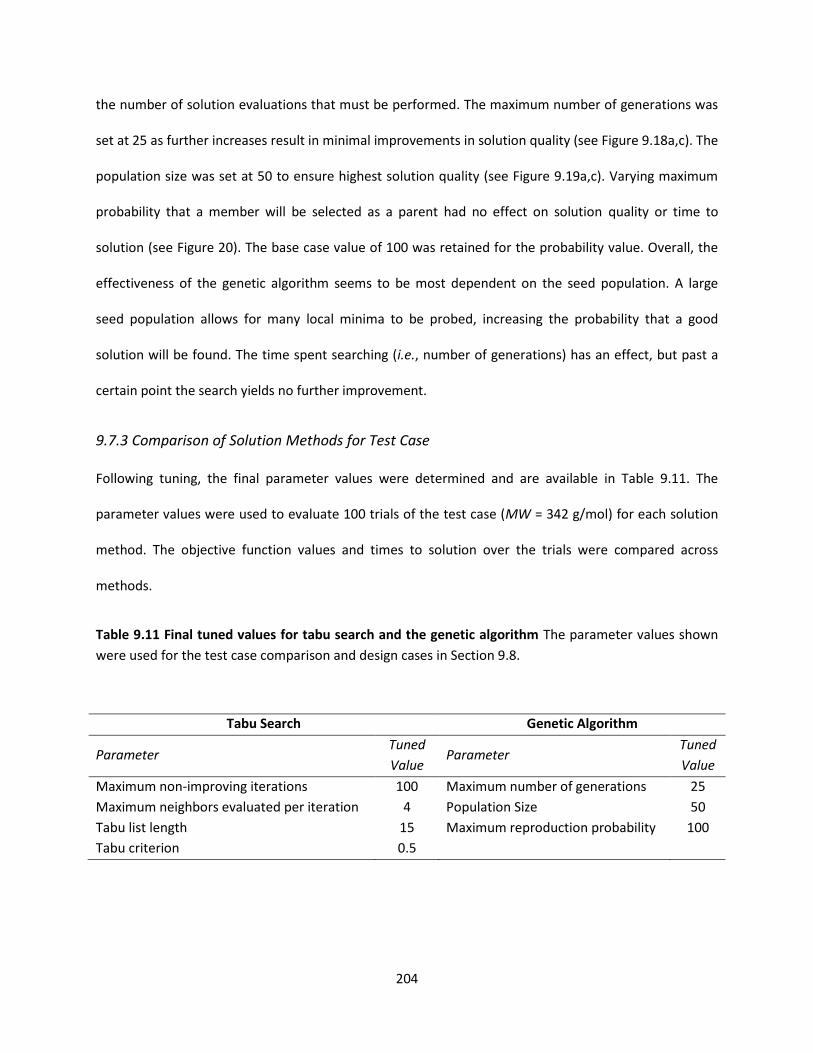
204
the number of solution evaluations that must be performed. The maximum number of generations was
set at 25 as further increases result in minimal improvements in solution quality (see Figure 9.18a,c). The
population size was set at 50 to ensure highest solution quality (see Figure 9.19a,c). Varying maximum
probability that a member will be selected as a parent had no effect on solution quality or time to
solution (see Figure 20). The base case value of 100 was retained for the probability value. Overall, the
effectiveness of the genetic algorithm seems to be most dependent on the seed population. A large
seed population allows for many local minima to be probed, increasing the probability that a good
solution will be found. The time spent searching (i.e., number of generations) has an effect, but past a
certain point the search yields no further improvement.
9.7.3 Comparison of Solution Methods for Test Case
Following tuning, the final parameter values were determined and are available in Table 9.11. The
parameter values were used to evaluate 100 trials of the test case (MW = 342 g/mol) for each solution
method. The objective function values and times to solution over the trials were compared across
methods.
Table 9.11 Final tuned values for tabu search and the genetic algorithm The parameter values shown
were used for the test case comparison and design cases in Section 9.8.
Tabu Search Genetic Algorithm
Parameter Tuned
Value Parameter
Tuned
Value
Maximum non-improving iterations 100 Maximum number of generations 25
Maximum neighbors evaluated per iteration 4 Population Size 50
Tabu list length 15 Maximum reproduction probability 100
Tabu criterion 0.5
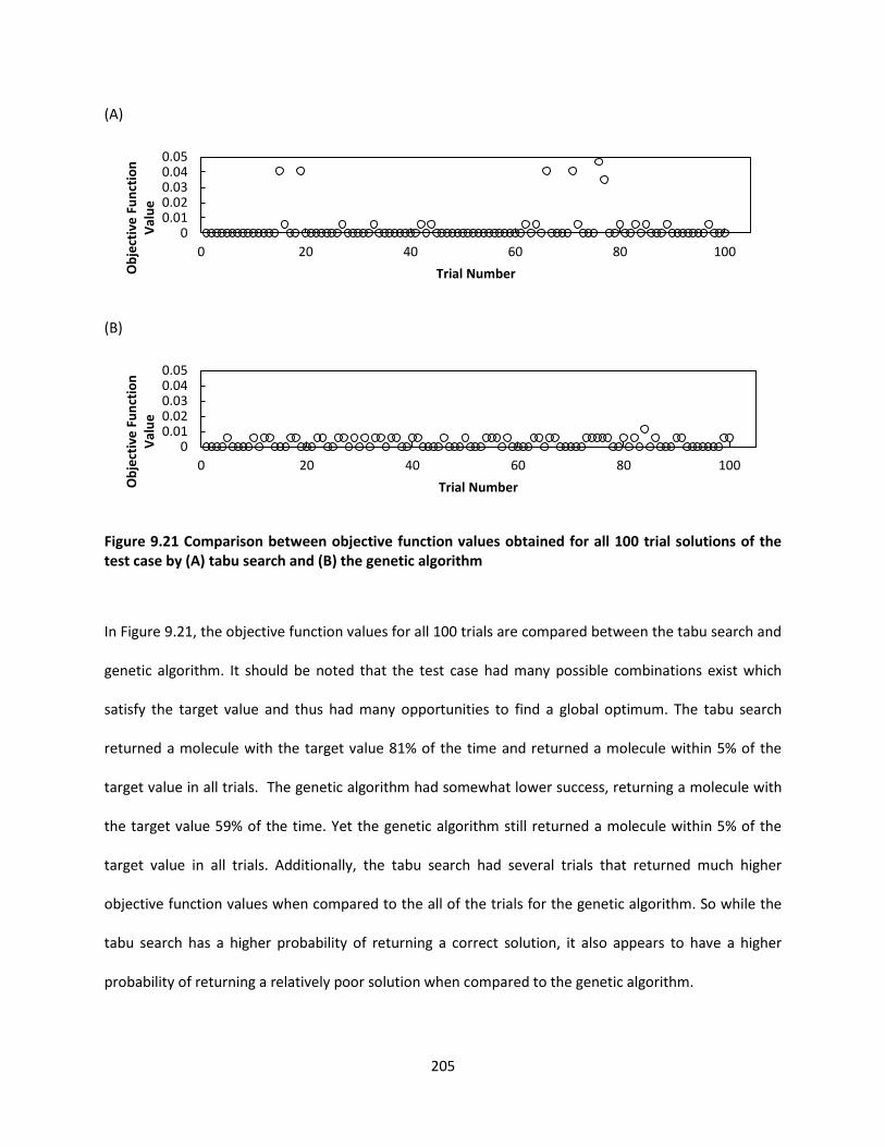
205
(A)
(B)
Figure 9.21 Comparison between objective function values obtained for all 100 trial solutions of the test case by (A) tabu search and (B) the genetic algorithm
In Figure 9.21, the objective function values for all 100 trials are compared between the tabu search and
genetic algorithm. It should be noted that the test case had many possible combinations exist which
satisfy the target value and thus had many opportunities to find a global optimum. The tabu search
returned a molecule with the target value 81% of the time and returned a molecule within 5% of the
target value in all trials. The genetic algorithm had somewhat lower success, returning a molecule with
the target value 59% of the time. Yet the genetic algorithm still returned a molecule within 5% of the
target value in all trials. Additionally, the tabu search had several trials that returned much higher
objective function values when compared to the all of the trials for the genetic algorithm. So while the
tabu search has a higher probability of returning a correct solution, it also appears to have a higher
probability of returning a relatively poor solution when compared to the genetic algorithm.
00.010.020.030.040.05
0 20 40 60 80 100
Ob
ject
ive
Fu
nct
ion
V
alu
e
Trial Number
00.010.020.030.040.05
0 20 40 60 80 100
Ob
ject
ive
Fu
nct
ion
V
alu
e
Trial Number

206
The times to solution for all 100 trials are compared between the tabu search and genetic algorithm in
Figure 9.22. The genetic algorithm had much less variability in time to solution as compared to tabu
search. The time to solution is also faster on average for the genetic algorithm. Neither observation is
surprising as the search effectively restarts during tabu search when a new best solution is identified.
The amount of restarts is random, leading to variability in time to solution. The tuning results suggest
that tabu search can return results with better objective function values while the genetic algorithm
returns results with significantly lower time to solution. To further compare the stochastic methods,
several design cases are considered in the following section.
(A)
(B)
Figure 9.22 Comparison between times to solution observed for all 100 trial solutions of the test case during (A) tabu search and (B) the genetic algorithm
010002000300040005000
0 20 40 60 80 100Tim
e t
o S
olu
tio
n
(mili
seco
nd
s)
Trial Number
010002000300040005000
0 20 40 60 80 100
Tim
e t
o S
olu
tio
n
(mili
seco
nd
s)
Trial Number
207
9.8 RESULTS FOR OPTIMAL DESIGN OF STABILIZERS FOR LYOPHILIZED PROTEIN FORMULATIONS
The tuned stochastic optimization methods presented in Section 9.7 were used in CAMD to obtain
optimal stabilizing excipient candidates for the property models outline in Section 9.5. The models for
individual proteins were chosen over the universal model given in Section 9.6 as the %Monomer models
dependent on excipient show superior fit and predictive capability. Therefore the models are good
examples to illustrate the ability of the CAMD methods to design excipients that optimally match the
given target value with low prediction error, as evaluated by prediction intervals. Design was limited to
carbohydrate excipients. Every design case was subjected to 100 trials. Results are compared across
stochastic optimization methods and also across proteins.
9.8.1 Comparison of CAMD Results Obtained by Tabu Search and a Genetic Algorithm
CAMD was used to generate optimal carbohydrate stabilizers for BSA, RNAse A, -amylase, ovalbumin
and trypsin inhibitor design cases. Solutions were obtained through use of the tuned stochastic
optimization methods presented in Section 9.7. The best solutions out of 100 runs of both solution
methods are displayed for each protein in Figures 9.23-9.27. The use of chirality connectivity indices in
the models allows chiral information to be determined for the solutions, giving an indication of three-
dimensional structure. A summary of the average objective function values and average times to
solution for all 100 runs is also presented in the figures.
For all design cases, the best results obtained from tabu search and the genetic algorithm had prediction
intervals that overlapped the target property value. Therefore, all of the best candidates returned
displayed predicted property values that were statistically similar to the desired target property value of
100% monomer remaining after lyophilization. Additionally, for each design case, the prediction
intervals for the best tabu search solution overlapped with the prediction intervals for the best genetic
algorithm solution. Despite returning solutions with objective function values that differed up to two
208
orders of magnitudes, both methods returned statistically similar solutions for all design cases. From the
basis of target property value returned by the best solution, both stochastic methods perform at a
similarly high level (i.e., both models return solutions that match the target property).
From case to case, the magnitude of prediction intervals varied. As the size of prediction intervals is
related to the expected error in the observed property value, solutions with small prediction intervals
are desired. Considering the best solutions only, tabu search returned solutions with smaller prediction
intervals for 3 cases (RNAse A, a-amylase and trypsin inhibitor) and the genetic algorithm returned
solutions with smaller prediction intervals for 2 cases (BSA and ovalbumin). The magnitude also varied
from case to case. In particular, the ovalbumin design case had solutions with extremely small prediction
intervals (see Figure 9.26). The magnitude of prediction intervals increases as the descriptors used in the
prediction diverge from the descriptor values used to build the predictive model. A quick look at the
best solutions reveals that many of the structures are quite different from the monosaccharaide,
disaccharaide, trisaccharaide and sugar alcohol structures used in model development. An exception
occurs in the ovalbumin design case. The tabu solution is very similar to maltitol and the genetic
algorithm solution is very similar to galactitol. Maltitol was used in model development and galactitol is
a stereoisomer of sorbitol and mannitol, both of which were used in model development. As a result,
the prediction intervals for both ovalbumin solutions are very small. In general, the prediction intervals
for all design cases are comparable to the average experimental standard deviation of 2.20%.
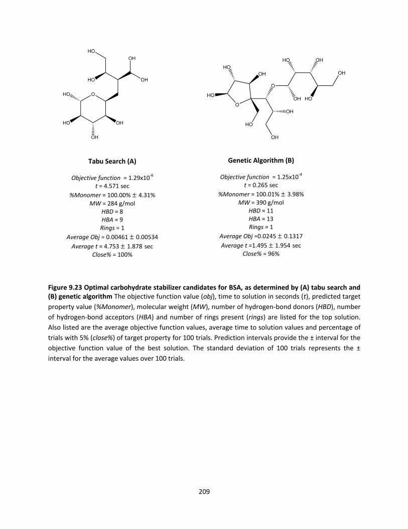
209
Figure 9.23 Optimal carbohydrate stabilizer candidates for BSA, as determined by (A) tabu search and (B) genetic algorithm The objective function value (obj), time to solution in seconds (t), predicted target
property value (%Monomer), molecular weight (MW), number of hydrogen-bond donors (HBD), number
of hydrogen-bond acceptors (HBA) and number of rings present (rings) are listed for the top solution.
Also listed are the average objective function values, average time to solution values and percentage of
trials with 5% (close%) of target property for 100 trials. Prediction intervals provide the ± interval for the
objective function value of the best solution. The standard deviation of 100 trials represents the ±
interval for the average values over 100 trials.
Tabu Search (A)
Objective function = 1.29x10⁻⁶
t = 4.571 sec
%Monomer = 100.00% ± 4.31%
MW = 284 g/mol HBD = 8
HBA = 9
Rings = 1
Average Obj = 0.00461 ± 0.00534
Average t = 4.753 ± 1.878 sec Close% = 100%
Genetic Algorithm (B)
Objective function = 1.25x10⁻⁴
t = 0.265 sec
%Monomer = 100.01% ± 3.98%
MW = 390 g/mol HBD = 11
HBA = 13
Rings = 1
Average Obj =0.0245 ± 0.1317
Average t =1.495 ± 1.954 sec Close% = 96%
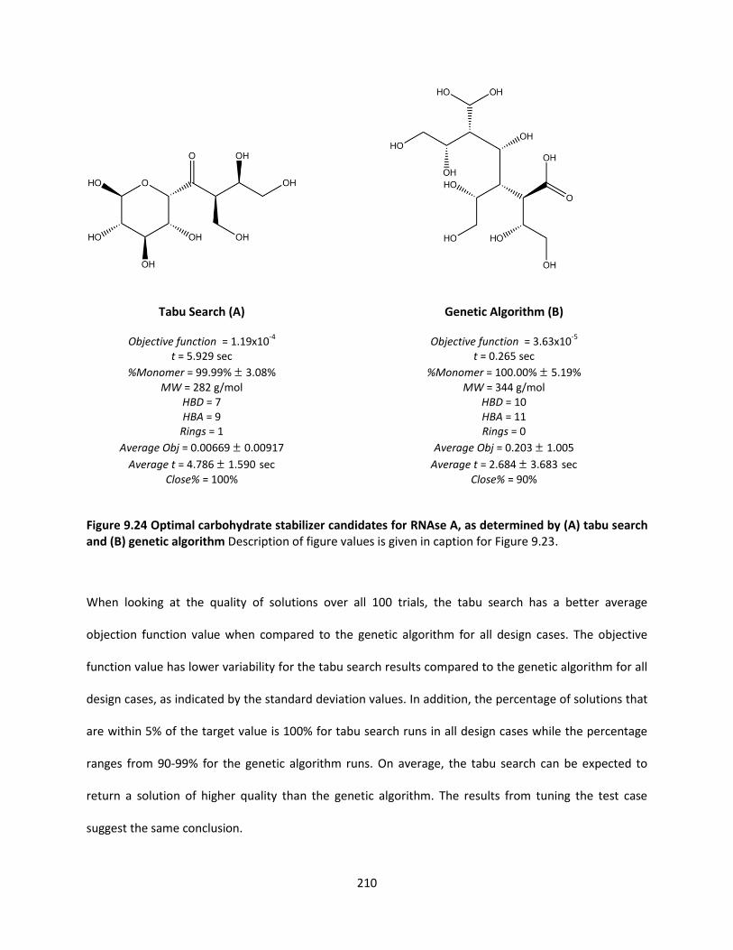
210
Tabu Search (A)
Objective function = 1.19x10⁻⁴
t = 5.929 sec
%Monomer = 99.99% ± 3.08%
MW = 282 g/mol HBD = 7
HBA = 9
Rings = 1
Average Obj = 0.00669 ± 0.00917
Average t = 4.786 ± 1.590 sec
Close% = 100%
Genetic Algorithm (B)
Objective function = 3.63x10⁻⁵
t = 0.265 sec
%Monomer = 100.00% ± 5.19%
MW = 344 g/mol HBD = 10
HBA = 11
Rings = 0
Average Obj = 0.203 ± 1.005
Average t = 2.684 ± 3.683 sec
Close% = 90%
Figure 9.24 Optimal carbohydrate stabilizer candidates for RNAse A, as determined by (A) tabu search and (B) genetic algorithm Description of figure values is given in caption for Figure 9.23.
When looking at the quality of solutions over all 100 trials, the tabu search has a better average
objection function value when compared to the genetic algorithm for all design cases. The objective
function value has lower variability for the tabu search results compared to the genetic algorithm for all
design cases, as indicated by the standard deviation values. In addition, the percentage of solutions that
are within 5% of the target value is 100% for tabu search runs in all design cases while the percentage
ranges from 90-99% for the genetic algorithm runs. On average, the tabu search can be expected to
return a solution of higher quality than the genetic algorithm. The results from tuning the test case
suggest the same conclusion.

211
Tabu Search (A)
Objective function = 1.83x10⁻⁵
t = 10.187 sec
%Monomer = 100.00 ± 1.50%
MW = 240 g/mol HBD = 7
HBA = 8
Rings = 1
Average Obj = 0.00153 ± 0.00162
Average t = 5.240 ± 1.985 sec Close% = 100%
Genetic Algorithm (B)
Objective function = 3.65x10⁻⁵
t = 0.265 sec
%Monomer = 100.00% ± 1.66%
MW = 284 g/mol HBD = 8
HBA = 9
Rings = 1
Average Obj =0.00536 ± 0.02107
Average t = 0.384 ± 0.397 sec Close% = 99%
Figure 9.25 Optimal carbohydrate stabilizer candidates for -amylase, as determined by (A) tabu search and (B) genetic algorithm Description of figure values is given in caption for Figure 9.23.
By method, the times to solution for the best solutions and the average times to solution were
comparable. Comparing methods, the genetic algorithm is an order of magnitude faster than tabu
search in determining a solution. The tabu search displays a higher variability in time to solution, as
indicated by the larger standard deviation values. As noted in the tuning results (see Section 9.7), the
tabu search effectively restarts when a new best solution is encountered. The number of times this
occurs is directly proportional to the time to solution. Average time to solution does vary somewhat as
the design case is varied, which likely indicates that more good solutions exist in the solution space for
some models as compared to others. If there are higher numbers of good solutions, the probability of
encountered a good solution is higher and the expected time to solution would be faster. Overall, the
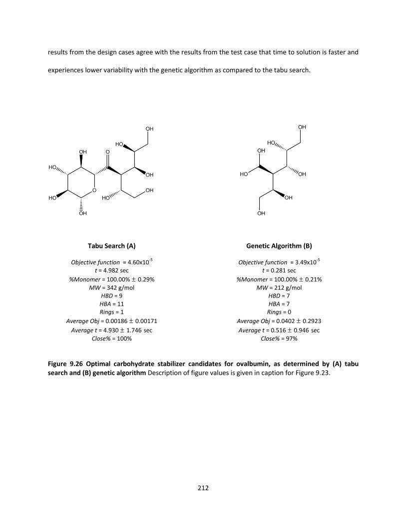
212
results from the design cases agree with the results from the test case that time to solution is faster and
experiences lower variability with the genetic algorithm as compared to the tabu search.
Tabu Search (A)
Objective function = 4.60x10⁻⁵
t = 4.982 sec
%Monomer = 100.00% ± 0.29%
MW = 342 g/mol HBD = 9
HBA = 11
Rings = 1
Average Obj = 0.00186 ± 0.00171
Average t = 4.930 ± 1.746 sec
Close% = 100%
Genetic Algorithm (B)
Objective function = 3.49x10⁻⁵
t = 0.281 sec
%Monomer = 100.00% ± 0.21%
MW = 212 g/mol HBD = 7
HBA = 7
Rings = 0
Average Obj = 0.0402 ± 0.2923
Average t = 0.516 ± 0.946 sec
Close% = 97%
Figure 9.26 Optimal carbohydrate stabilizer candidates for ovalbumin, as determined by (A) tabu search and (B) genetic algorithm Description of figure values is given in caption for Figure 9.23.
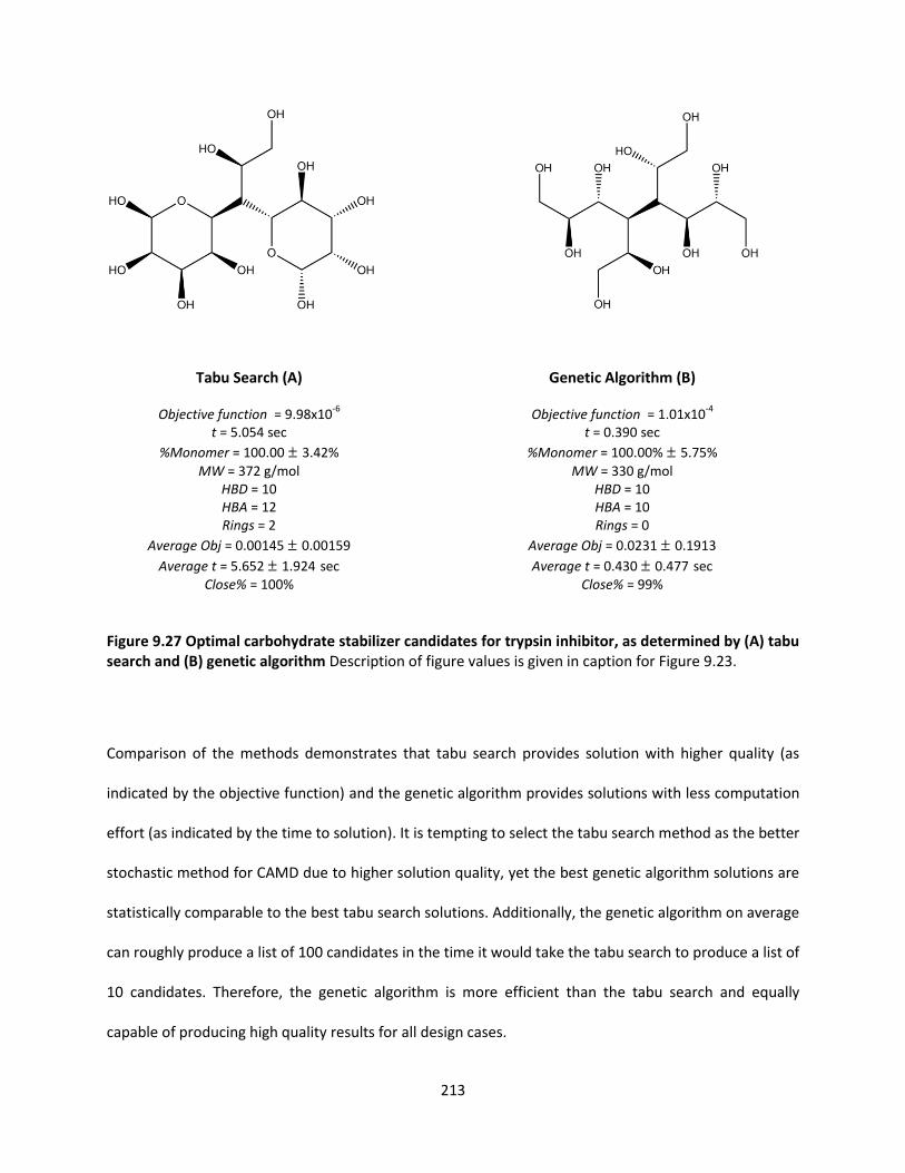
213
Tabu Search (A)
Objective function = 9.98x10⁻⁶
t = 5.054 sec
%Monomer = 100.00 ± 3.42%
MW = 372 g/mol HBD = 10
HBA = 12
Rings = 2
Average Obj = 0.00145 ± 0.00159
Average t = 5.652 ± 1.924 sec Close% = 100%
Genetic Algorithm (B)
Objective function = 1.01x10⁻⁴
t = 0.390 sec
%Monomer = 100.00% ± 5.75%
MW = 330 g/mol HBD = 10
HBA = 10
Rings = 0
Average Obj = 0.0231 ± 0.1913
Average t = 0.430 ± 0.477 sec Close% = 99%
Figure 9.27 Optimal carbohydrate stabilizer candidates for trypsin inhibitor, as determined by (A) tabu search and (B) genetic algorithm Description of figure values is given in caption for Figure 9.23.
Comparison of the methods demonstrates that tabu search provides solution with higher quality (as
indicated by the objective function) and the genetic algorithm provides solutions with less computation
effort (as indicated by the time to solution). It is tempting to select the tabu search method as the better
stochastic method for CAMD due to higher solution quality, yet the best genetic algorithm solutions are
statistically comparable to the best tabu search solutions. Additionally, the genetic algorithm on average
can roughly produce a list of 100 candidates in the time it would take the tabu search to produce a list of
10 candidates. Therefore, the genetic algorithm is more efficient than the tabu search and equally
capable of producing high quality results for all design cases.

214
9.8.2 Comparison of CAMD Results as a Function of Protein Included in the Formulation
A comparison of solutions between each design case (i.e., protein) was performed to determine if
certain chemical characteristics were preferred by one protein over another. The chemical properties
used for comparison were molecular weight (MW), number of hydrogen bond donors (HBD), number of
hydrogen bond acceptors (HBA) and number of rings present (rings). The comparison of average CAMD
solution properties by protein is given in Figure 9.28.
Comparison of results indicates that no significant difference in the properties considered exist across
proteins. The solutions for both stochastic methods average to a monosaccharide (1 ring) with six to
seven hydrogen bond donors, eight to nine hydrogen bond acceptors and a molecular weight less than
300 g/mol. The disaccharides sucrose and trehalose are often cited as effective lyoprotectants
(Schwegman, Hardwick et al. 2005). The average solution property values are lower than the property
values observed for sucrose and trehalose, which are isomers and have molecular weights of 342 g/mol,
eight hydrogen bond donors and eleven hydrogen bond donors. Of the best solutions presented in
Section 9.8.1, only one solution contained two rings (see Figure 9.27a). All other solutions contained
either one ring or no rings.

215
(A) (B)
(C) (D)
Figure 9.28 Comparison across protein models of average chemical information for solutions derived by both tabu search and genetic algorithm The information used for comparison are (A) molecular
weight (g/mol), (B) number of rings, (C) number of hydrogen bond donors, and (D) number of hydrogen
bond acceptors. Error bars represent the standard deviation of 100 trials for each case.
The three-dimensional conformation appears to be more important than the chemical properties
considered for obtaining 100% monomer remaining after lyophilization. By incorporating chiral
connectivity indices in the %Monomer property models, three-dimensional information is captured.
Only nine building block groups are used in the determination of all the solutions presented. Yet, the
050
100150200250300350400450
MW
(g/
mo
l)
Tabu
GA
00.20.40.60.8
11.21.41.61.8
2
# o
f R
ings
Tabu
GA
0
2
4
6
8
10
12
# o
f H
ydro
gen
Bo
nd
Do
no
rs
Tabu
GA
0
2
4
6
8
10
12
14
# o
f H
ydro
gen
Bo
nd
Acc
ep
tors
Tabu
GA

216
inclusion of chirality information vastly increases the number of possible solutions and is the overriding
factor in the design of optimal solutions. The models and CAMD results here present the first use of
chiral connectivity indices in CAMD and the first use of topological descriptors to provide CAMD
solutions with three-dimensional structural information. It is important to note that the solutions
provided were not designed using all relevant excipient properties and should therefore not be
considered final candidates for immediate inclusion in lyophilized protein formulations. However, both
stochastic methods are able to quickly generate a large list of optimal candidates that can be further
screened in a post-design phase, which may include any combination of additional property models,
molecular simulations and experiments that are deemed necessary. The work here provides a starting
point for the CAMD of excipients with three-dimensional structural information for stabilization of
lyophilized proteins.
217
10.0 CONCLUSIONS AND FUTURE RECOMMENDATIONS
The work presented here describes the comprehensive development of CAMD methods with
applications towards bioengineering, namely the design of ionic liquid media for bioseparations and the
design of excipients for lyophilized protein formulations. The pre-design approach to CAMD is concerned
with the determination of systems of interest and the acquisition of data for property of interests.
Where available, data was collected from literature to build the models developed here. For prediction
of monomeric protein remaining after lyophilization, the collection of experimental data was required.
The design phase of CAMD is comprised of two sub-problems. The forward problem is concerned with
property model development, linking structure to properties of interest. Several approaches novel to
CAMD were employed to better provide models of sufficient fit and predictive power. Descriptor
selection was used when applicable to provide models with sufficient fit while avoiding overfitting.
Exhaustive selection was found to be superior to forward selection when developing models describing
%Monomer as a function of protein structure. The use of cross-validation has been used previously in
CAMD (Eslick, Ye et al. 2009), but the approach was furthered here with the use of K-fold validation to
more significantly probe predictive capability of models describing %Monomer as a function of excipient
structure. Additionally, the use of Q2 as an indicator of predictive power was illustrated with poor Q2
values leading to predicted ionic liquid toxicity values with large prediction intervals. Molecular
descriptors novel to CAMD were used for the models describing %Monomer as a function of excipient
structure, which provided chirality information to help distinguish between molecules. By using chiral
connectivity indices, some three-dimensional structural information was captured using only a two-
dimensional molecular representation.
The reverse problem of the CAMD aims to propose molecular structures that optimally match given
target property values. Molecular candidates to the ionic liquid and excipient design problems were
218
proposed using a variety of solution approaches. Deterministic methods were used to solve for ionic
liquid entrainers for separation of azeotropic mixtures. Tabu search, a stochastic method, was used to
design ionic liquid extractants and excipients with optimal glass forming properties. Novel to the work
presented here, two stochastic optimization methods (i.e., tabu search and genetic algorithm) were
tuned for CAMD applications. The stochastic methods were then used to design carbohydrate stabilizers
for lyophilized protein formulations. Evaluation of the two methods showed that tabu search had longer
time to solutions but higher solution quality and consistency when compared to the genetic algorithm.
However when comparing the best solutions from each method, the predicted target values were
similar as indicated by overlapping prediction intervals. Use of prediction intervals are original to the
CAMD approaches used here and help to provide a statistical means of comparison between solutions.
By incorporating chiral connectivity indices in the design of stabilizing excipients, three-dimensional
structural information for design solutions was provided for the first time in CAMD approaches through
use of only two-dimensional structural information.
The post-design of CAMD aims to further screen and establish good candidates for a given application.
The coupling of product and process design allowed for the design of ionic liquid entrainers and
azeotropic separation processes with near-optimal performance in terms of energy requirements. Final
ionic liquid separation process results were shown to require less energy to perform separations than
systems using entrainers that were not rationally designed. Molecular simulation was investigated as a
tool to approximate hydrogen-deuterium exchange experiments and gleam information on possible
protein-excipient interactions. Use of simulation results are likely insufficient to guide design at the
current state of implementation. A better use of molecular simulation is likely to be as a post-design
screening tool to further narrow down an excipient candidate list for a given lyophilized protein
formulation.

219
Moving forward, more property models are needed for the examples considered to better generate a
list of candidates that would be expected to perform successfully. For example, human toxicity would be
important for the design of excipients for protein drug formulations. Additionally, several of the design
solutions are reducing sugars, which would not be acceptable for protein formulations. Rules for group
addition or improved penalty functions could be employed to prevent reducing sugars from being
selected as solutions. In several of the design examples, the error in property prediction of %Monomer
exceeds what would be acceptable from the viewpoint of the biopharmaceutical industry. A multi-
objective optimization problem could be formulated to minimize both differences between target and
predicted properties along with prediction intervals of predicted properties. Such a problem formulation
would insure that solutions are returned where confidence in the predicted property values is high. For
prediction of glass transitions, multiple transitions may occur in a sugar. Improvement to glass transition
properties could include the prediction of polymorphic systems where multiple transitions would be
expected to occur. The shift from one-dimensional (e.g., group contribution) and two-dimensional
descriptors towards three-dimensional or quantum descriptors will likely provide better property
prediction and more accurate design results in future CAMD applications.
Tuning of the tabu search and genetic algorithm was performed on a basic level. Future work in tuning
and increased levels of sophistication in the design algorithms will be useful in improving algorithm
efficiency and solution quality. For example, mutation rate and crossover rate were randomly selected
in the genetic algorithm. Further tuning could identify rates that were more useful for CAMD.
Additionally, the tuning results presented are dependent on the base values of parameters used for
tuning. It is possible that the base value for a parameter could have such a value that the parameter
overwhelmed the effects of other parameters. Further investigation into the base parameter values and
their effect on the final chosen tuned values would be of interest. An especially promising area of
algorithm development is the parallelization of stochastic optimization methods, which is expected to

220
provide substantial improvements to the computational costs of performing CAMD. As molecular
complexity increases, the resulting combinatorial search space could warrant the need for vastly reduce
search times that would be proffered by parallelization. The parallelization of both stochastic solution
methods would also be of interest from the point of view of a pure scientific curiosity. Combination of
the design process with a database search offers a promising avenue of future post-design methods. For
example, a molecule that is design could be used to identify similar molecules in online structure
databases, such as PubChem. Similarity searches would provide a way to experimentally validate CAMD
design results without the time and complexity that would result from chemical synthesis of the design
solutions. Information from experimental validation could be used to further improve property models
and design methods. Such an integrated experimental-computational CAMD approach would be
instrumental in the identification of molecule candidates for use in a variety of bioengineering
applications, including the lyophilized protein formulation design and ionic liquid solvent design cases
considered here.
221
REFERENCES
Akamatsu, M. (2002). "Current State and Perspectives of 3D-QSAR." Current Topics in Medicinal Chemistry 2(12): 1381-1394.
Anfinsen, C. B. (1972). "The formation and stabilization of protein structure." Biochem. J. 128(4): 737-749.
Ann, E. V., J. B. Nicholas and D. R. Robin (2012). Preface. Ionic Liquids: Science and Applications, American Chemical Society. 1117: ix-x.
Arakawa, T., D. Ejima, T. Li and J. S. Philo (2010). "The critical role of mobile phase composition in size exclusion chromatography of protein pharmaceuticals." Journal of Pharmaceutical Sciences 99(4): 1674-1692.
Arakawa, T. and Y. Kita (2000). "Stabilizing effects of caprylate and acetyltryptophanate on heat-induced aggregation of bovine serum albumin." Biochimica et Biophysica Acta (BBA) - Protein Structure and Molecular Enzymology 1479(1–2): 32-36.
Arakawa, T. and S. N. Timasheff (1982). "Stabilization of protein structure by sugars." Biochemistry 21(25): 6536-6544.
Awad, W. H., J. W. Gilman, M. Nyden, R. H. Harris Jr, T. E. Sutto, J. Callahan, P. C. Trulove, H. C. DeLong and D. M. Fox (2004). "Thermal degradation studies of alkyl-imidazolium salts and their application in nanocomposites." Thermochimica Acta 409(1): 3-11.
B c , T. (199 ). Evolutionary algorithms in theory and practice : evolution strategies, evolutionary programming, genetic algorithms. New York, Oxford University Press.
Barton, A. F. M. (1991). CRC handbook of solubility parameters and other cohesion parameters. Boca Raton, Fla., CRC Press.
Barton, P. (2000). "Solvent recovery opportunities in the pharmaceutical industry." Current Opinion in Drug Discovery & Development 3(6): 707 - 713.
Bek-Pedersen, E., R. Gani and O. Levaux (2000). "Determination of optimal energy efficient separation schemes based on driving forces." Computers & Chemical Engineering 24(2-7): 253-259.
Bicerano, J. (2002). Prediction of polymer properties. New York, Marcel Dekker. Bondi, A. (1964). "van der Waals Volumes and Radii." The Journal of Physical Chemistry 68(3): 441-451. Camarda, K. V. and C. D. Maranas (1999). "Optimization in Polymer Design Using Connectivity Indices."
Industrial & Engineering Chemistry Research 38(5): 1884-1892. Camarda, K. V. and P. Sunderesan (2005). "An Optimization Approach to the Design of Value-Added
Soybean Oil Products." Industrial & Engineering Chemistry Research 44(12): 4361-4367. Carpenter, J. F. and J. H. Crowe (1989). "An infrared spectroscopic study of the interactions of
carbohydrates with dried proteins." Biochemistry 28(9): 3916-3922. Carpenter, J. F., T. W. Randolph, W. Jiskoot, D. J. A. Crommelin, C. R. Middaugh and G. Winter (2010).
"Potential inaccurate quantitation and sizing of protein aggregates by size exclusion chromatography: Essential need to use orthogonal methods to assure the quality of therapeutic protein products." Journal of Pharmaceutical Sciences 99(5): 2200-2208.
Carpenter, J. F., T. W. Randolph, W. Jiskoot, D. J. A. Crommelin, C. R. Middaugh, G. Winter, Y.-X. Fan, S. Kirshner, D. Verthelyi, S. Kozlowski, K. A. Clouse, P. G. Swann, A. Rosenberg and B. Cherney (2009). "Overlooking subvisible particles in therapeutic protein products: Gaps that may compromise product quality." Journal of Pharmaceutical Sciences 98(4): 1201-1205.
Chang, B. S., B. S. Kendrick and J. F. Carpenter (1996). "Surface-induced denaturation of proteins during freezing and its inhibition by surfactants." Journal of Pharmaceutical Sciences 85(12): 1325-1330.

222
Cheng, F., J. Shen, X. Luo, W. Zhu, J. Gu, R. Ji, H. Jiang and K. Chen (2002). "Molecular docking and 3-D-QSAR studies on the possible antimalarial mechanism of artemisinin analogues." Bioorganic & Medicinal Chemistry 10(9): 2883-2891.
Chennamsetty, N., V. Voynov, V. Kayser, B. Helk and B. L. Trout (2009). "Design of therapeutic proteins with enhanced stability." Proceedings of the National Academy of Sciences 106(29): 11937-11942.
Chi, E., S. Krishnan, T. Randolph and J. Carpenter (2003). "Physical Stability of Proteins in Aqueous Solution: Mechanism and Driving Forces in Nonnative Protein Aggregation." Pharmaceutical Research 20(9): 1325-1336.
Chi, E. Y., S. Krishnan, T. W. Randolph and J. F. Carpenter (2003). "Physical stability of proteins in aqueous solution: Mechanism and driving forces in nonnative protein aggregation." Pharmaceutical Research 20(9): 1325-1336.
Chowdhury, S. K., V. Katta and B. T. Chait (1990). "Probing conformational changes in proteins by mass spectrometry." Journal of the American Chemical Society 112(24): 9012-9013.
Clas, S. D., R. Faizer, R. E. O'Connor and E. B. Vadas (1995). "Quantification of crystallinity in blends of lyophilized and crystalline MK-0591 using x-ray powder diffraction." International Journal of Pharmaceutics 121(1): 73-79.
Cleland, J. L., R. S. Langer and American Chemical Society. Division of Biochemical Technology. (1994). Formulation and delivery of proteins and peptides. Washington, DC, American Chemical Society.
Conchillo-Sole, O., N. de Groot, F. Aviles, J. Vendrell, X. Daura and S. Ventura (2007). "AGGRESCAN: a server for the prediction and evaluation of "hot spots" of aggregation in polypeptides." BMC Bioinformatics 8(1): 65.
Conchillo-Sole, O., N. S. de Groot, F. X. Aviles, J. Vendrell, X. Daura and S. Ventura (2007). "AGGRESCAN: a server for the prediction and evaluation of "hot spots" of aggregation in polypeptides." BMC Bioinformatics 8: 65.
Consonni, V. and R. Todeschini (2000). Handbook of molecular descriptors. Weinheim ; Chichester, Wiley-VCH.
Conte, E., R. Gani, Y. S. Cheng and K. M. Ng (2012). "Design of formulated products: Experimental component." AIChE Journal 58(1): 173-189.
Conte, E., R. Gani and K. M. Ng (2011). "Design of formulated products: A systematic methodology." AIChE Journal 57(9): 2431-2449.
Costantino, H. R. and M. J. Pikal (2004). Lyophilization of biopharmaceuticals. Arlington, VA, AAPS Press. Cottone, G., G. Ciccotti and L. Cordone (2002). "Protein--trehalose--water structures in trehalose coated
carboxy-myoglobin." The Journal of Chemical Physics 117(21): 9862-9866. Crowe, J. H., J. F. Carpenter and L. M. Crowe (1998). "The role of vitrification in anhydrobiosis." Annual
Review of Physiology 60(1): 73-103. Cussler, E. L. and G. D. Moggridge (2011). Chemical product design. Cambridge ; New York, Cambridge
University Press. D. Holbrey, J. and K. R. Seddon (1999). "The phase behaviour of 1-alkyl-3-methylimidazolium
tetrafluoroborates; ionic liquids and ionic liquid crystals." Journal of the Chemical Society, Dalton Transactions(13): 2133-2140.
Dalgaard, P. (2008). Introductory Statistics with R. New York, NY, Springer Science+Business Media, LLC. Domanska, U. and A. Marciniak (2008). "Measurements of activity coefficients at infinite dilution of
aromatic and aliphatic hydrocarbons, alcohols, and water in the new ionic liquid [EMIM][SCN] using GLC." The Journal of Chemical Thermodynamics 40(5): 860-866.
Doma s a, U. and A. Marcinia ( 007). "Activity Coefficients at Infinite Dilution Measurements for Organic Solutes and Water in the Ionic Liquid 1-Ethyl-3-methylimidazolium Trifluoroacetate." The Journal of Physical Chemistry B 111(41): 11984-11988.

223
Doma ska, U. and A. Marciniak (2008). "Activity Coefficients at Infinite Dilution Measurements for Organic Solutes and Water in the Ionic Liquid 1-Butyl-3-methylimidazolium Trifluoromethanesulfonate." The Journal of Physical Chemistry B 112(35): 11100-11105.
Duran, M. and I. Grossmann (1986). "An outer-approximation algorithm for a class of mixed-integer nonlinear programs." Mathematical Programming 36(3): 307-339.
Duy, C. and J. Fitter ( 005). "Thermostability of Irreversible Unfolding α-Amylases Analyzed by Unfolding Kinetics." Journal of Biological Chemistry 280(45): 37360-37365.
Eden, M. R., S. B. Jørgensen, R. Gani and M. M. El-Halwagi (2004). "A novel framework for simultaneous separation process and product design." Chemical Engineering and Processing: Process Intensification 43(5): 595-608.
Edgar, T. F., D. M. Himmelblau and L. S. Lasdon (2001). Optimization of chemical processes. New York, McGraw-Hill.
Eike, D. M., J. F. Brennecke and E. J. Maginn (2004). "Predicting Infinite-Dilution Activity Coefficients of Organic Solutes in Ionic Liquids." Industrial & Engineering Chemistry Research 43(4): 1039-1048.
Eljack, F. T. and M. R. Eden (2008). "A systematic visual approach to molecular design via property clusters and group contribution methods." Computers & Chemical Engineering 32(12): 3002-3010.
Engelsman, J., P. Garidel, R. Smulders, H. Koll, B. Smith, S. Bassarab, A. Seidl, O. Hainzl and W. Jiskoot (2011). "Strategies for the Assessment of Protein Aggregates in Pharmaceutical Biotech Product Development." Pharmaceutical Research 28(4): 920-933.
Eslick, J. (2009). Molecular Design of Crosslinked Copolymers. Department of Chemical and Petroleum Engineering, University of Kansas. PhD in Chemical Engineering.
Eslick, J. C., Q. Ye, J. Park, E. M. Topp, P. Spencer and K. V. Camarda (2009). "A computational molecular design framework for crosslinked polymer networks." Computers & Chemical Engineering 33(5): 954-963.
Eslick, J. C., Q. Ye, J. Park, E. M. Topp, P. Spencer and K. V. Camarda (2009). "A computational molecular design framework for crosslinked polymer networks." Computers and Chemical Engineering 33(5): 954-963.
Ferguson, T. Linear Programming: A Concise Introduction. Floudas, C. A. (1995). Nonlinear and mixed-integer optimization: fundamentals and applications, Oxford
University Press. Fredenslund, A., J. Gmehling and P. Rasmussen (1977). Vapor-liquid equilibria using UNIFAC: a group
contribution method, Elsevier Scientific Pub. Co. Fredlake, C. P., J. M. Crosthwaite, D. G. Hert, S. N. V. K. Aki and J. F. Brennecke (2004). "Thermophysical
Properties of Imidazolium-Based Ionic Liquids." Journal of Chemical & Engineering Data 49(4): 954-964.
Fung, J., A. A. Darabie and J. McLaurin (2005). "Contribution of simple saccharides to the stabilization of amyloid structure." Biochemical and Biophysical Research Communications 328(4): 1067-1072.
Gangasharan and S. S. N. Murthy (1995). "Nature of the Relaxation Processes in the Supercooled Liquid and Glassy States of Some Carbohydrates." The Journal of Physical Chemistry 99(32): 12349-12354.
Gangu, S. A., L. R. Weatherley and A. M. Scurto (2009). "Whole-Cell Biocatalysis with Ionic Liquids." Current Organic Chemistry 13(13): 1242-1258.
Gani, R. (2004). "Chemical product design: challenges and opportunities." Computers & Chemical Engineering 28(12): 2441-2457.
Gani, R. and E. Bek-Pedersen (2000). "Simple new algorithm for distillation column design." AIChE Journal 46(6): 1271-1274.
224
Gani, R. and E. A. Brignole (1983). "Molecular design of solvents for liquid extraction based on UNIFAC." Fluid Phase Equilibria 13(0): 331-340.
Gani, R., P. M. Harper and M. Hostrup (2005). "Automatic Creation of Missing Groups through Connectivity Index for Pure-Component Property Prediction." Industrial & Engineering Chemistry Research 44(18): 7262-7269.
Gani, R., G. Hytoft, C. Jaksland and A. K. Jensen (1997). "An integrated computer aided system for integrated design of chemical processes." Computers & Chemical Engineering 21(10): 1135-1146.
Gani, R., B. Nielsen and A. Fredenslund (1991). "A group contribution approach to computer-aided molecular design." AIChE Journal 37(9): 1318-1332.
Gani, R., N. Tzouvaras, P. Rasmussen and A. Fredenslund (1989). "Prediction of gas solubility and vapor-liquid equilibria by group contribution." Fluid Phase Equilibria 47(2-3): 133-152.
Gardas, R. L. and J. o. A. P. Coutinho (2008). "A Group Contribution Method for Heat Capacity Estimation of Ionic Liquids." Industrial & Engineering Chemistry Research 47(15): 5751-5757.
Ge, M.-L. and L.-S. Wang (2008). "Activity Coefficients at Infinite Dilution of Polar Solutes in 1-Butyl-3-methylimidazolium Trifluoromethanesulfonate Using Gas–Liquid Chromatography." Journal of Chemical & Engineering Data 53(3): 846-849.
Ge, M.-L., L.-S. Wang, M.-Y. Li and J.-S. Wu (2007). "Activity Coefficients at Infinite Dilution of Alkanes, Alkenes, and Alkyl Benzenes in 1-Butyl-3-methylimidazolium Trifluoromethanesulfonate Using Gas− iquid Chromatography." Journal of Chemical & Engineering Data 52(6): 2257-2260.
Ge, M.-L., L.-S. Wang, J.-S. Wu and Q. Zhou (2008). "Activity Coefficients at Infinite Dilution of Organic Solutes in 1-Ethyl-3-methylimidazolium Tetrafluoroborate Using Gas− iquid Chromatography." Journal of Chemical & Engineering Data 53(8): 1970-1974.
Glover, F. (1989). "Tabu search—part I." ORSA Journal on computing 1(3): 190-206. Gmehling, J., Menke, J., Krafczyk, J., Fischer, K. (1994). Azeotropic Data. Weinheim, Germany, VCH. Golbraikh, A., D. Bonchev and A. Tropsha (2001). "Novel Chirality Descriptors Derived from Molecular
Topology." Journal of Chemical Information and Computer Sciences 41(1): 147-158. Golbraikh, A., M. Shen, Z. Xiao, Y.-D. Xiao, K.-H. Lee and A. Tropsha (2003). "Rational selection of training
and test sets for the development of validated QSAR models." Journal of Computer-Aided Molecular Design 17(2-4): 241-253.
Goodsell, D. S., G. M. Morris and A. J. Olson (1996). "Automated docking of flexible ligands: Applications of autodock." Journal of Molecular Recognition 9(1): 1-5.
Gsponer, J. and M. Vendruscolo (2006). "Theoretical approaches to protein aggregation." Protein and peptide letters 13(3): 287-293.
Hackel, C., T. Zinkevich, P. Belton, A. Achilles, D. Reichert and A. Krushelnitsky (2012). "The trehalose coating effect on the internal protein dynamics." Physical Chemistry Chemical Physics 14(8): 2727-2734.
Harper, P. M. and R. Gani (2000). "A multi-step and multi-level approach for computer aided molecular design." Computers & Chemical Engineering 24(2–7): 677-683.
Harper, P. M., R. Gani, P. Kolar and T. Ishikawa (1999). "Computer-aided molecular design with combined molecular modeling and group contribution." Fluid Phase Equilibria 158–160(0): 337-347.
Heintz, A., L. M. Casás, I. A. Nesterov, V. N. Emel'yanenko and S. P. Verevkin (2005). "Thermodynamic Properties of Mixtures Containing Ionic Liquids. 5. Activity Coefficients at Infinite Dilution of Hydrocarbons, Alcohols, Esters, and Aldehydes in 1-Methyl-3-butyl-imidazolium Bis(trifluoromethyl-sulfonyl) Imide Using Gas− iquid Chromatography." Journal of Chemical & Engineering Data 50(5): 1510-1514.

225
Heintz, A., D. V. Kulikov and S. P. Verevkin (2001). "Thermodynamic Properties of Mixtures Containing Ionic Liquids. 1. Activity Coefficients at Infinite Dilution of Alkanes, Alkenes, and Alkylbenzenes in 4-Methyl-n-butylpyridinium Tetrafluoroborate Using Gas− iquid Chromatography." Journal of Chemical & Engineering Data 46(6): 1526-1529.
Heintz, A., D. V. Kulikov and S. P. Verevkin (2002). "Thermodynamic properties of mixtures containing ionic liquids. Activity coefficients at infinite dilution of polar solutes in 4-methyl- N-butyl-pyridinium tetrafluoroborate using gas-liquid chromatography." The Journal of Chemical Thermodynamics 34(8): 1341-1347.
Heintz, A., T. V. Vasiltsova, J. Safarov, E. Bich and S. P. Verevkin (2006). "Thermodynamic Properties of Mixtures Containing Ionic Liquids. 9. Activity Coefficients at Infinite Dilution of Hydrocarbons, Alcohols, Esters, and Aldehydes in Trimethyl-butylammonium Bis(trifluoromethylsulfonyl) Imide Using Gas− iquid Chromatography and Static Method." Journal of Chemical & Engineering Data 51(2): 648-655.
Heintz, A. and S. P. Verevkin (2005). "Thermodynamic Properties of Mixtures Containing Ionic Liquids. 6. Activity Coefficients at Infinite Dilution of Hydrocarbons, Alcohols, Esters, and Aldehydes in 1-Methyl-3-octyl-imidazolium Tetrafluoroborate Using Gas− iquid Chromatography." Journal of Chemical & Engineering Data 50(5): 1515-1519.
Heintz, A., S. P. Verevkin and D. Ondo (2006). "Thermodynamic Properties of Mixtures Containing Ionic Liquids. 8. Activity Coefficients at Infinite Dilution of Hydrocarbons, Alcohols, Esters, and Aldehydes in 1-Hexyl-3-methylimidazolium Bis(trifluoromethylsulfonyl) Imide Using Gas− iquid Chromatography." Journal of Chemical & Engineering Data 51(2): 434-437.
Hetényi, C. and D. van der Spoel (2002). "Efficient docking of peptides to proteins without prior knowledge of the binding site." Protein Science 11(7): 1729-1737.
Hetényi, C. and D. van der Spoel (2006). "Blind docking of drug-sized compounds to proteins with up to a thousand residues." FEBS Letters 580(5): 1447-1450.
Holland, J. H. (1975). Adaptation in natural and artificial systems : an introductory analysis with applications to biology, control, and artificial intelligence. Ann Arbor, University of Michigan Press.
HSL. (2011). "A collection of Fortran codes for large scale scientific computation." from http://www.hsl.rl.ac.uk.
Huang, H.-J., S. Ramaswamy, U. W. Tschirner and B. V. Ramarao (2008). "A review of separation technologies in current and future biorefineries." Separation and Purification Technology 62(1): 1-21.
Huey, R., G. M. Morris, A. J. Olson and D. S. Goodsell (2007). "A semiempirical free energy force field with charge-based desolvation." Journal of Computational Chemistry 28(6): 1145-1152.
Irbäck, A. and S. Mohanty (2006). "PROFASI: A Monte Carlo simulation package for protein folding and aggregation." Journal of Computational Chemistry 27(13): 1548-1555.
Jerina, D. M., J. W. Daly, A. M. Jeffrey and D. T. Gibson (1971). "Cis-1,2-dihydroxy-1,2-dihydronaphthalene: A bacterial metabolite from naphthalene." Archives of Biochemistry and Biophysics 142(1): 394-396.
Joback, K. G. and R. C. Reid (1987). "Estimation of pure-component properties from group-contribution." Chemical Engineering Communications 57(1): 233 - 243.
Karunanithi, A. T., L. E. K. Achenie and R. Gani (2006). "A computer-aided molecular design framework for crystallization solvent design." Chemical Engineering Science 61(4): 1247-1260.
Katayama, D. S., J. F. Carpenter, K. P. Menard, M. C. Manning and T. W. Randolph (2009). "Mixing properties of lyophilized protein systems: A spectroscopic and calorimetric study." Journal of Pharmaceutical Sciences 98(9): 2954-2969.

226
Katayama, D. S., R. Nayar, D. K. Chou, J. Campos, J. Cooper, D. G. Vander Velde, L. Villarete, C. P. Liu and M. Cornell Manning (2005). "Solution behavior of a novel type 1 interferon, interferon-τ." Journal of Pharmaceutical Sciences 94(12): 2703-2715.
Kato, R. and J. Gmehling (2004). "Activity coefficients at infinite dilution of various solutes in the ionic liquids [MMIM]+[CH3SO4]-, [MMIM]+[CH3OC2H4SO4]-, [MMIM]+[(CH3)2PO4]-, [C5H5NC2H5]+[(CF3SO2)2N]- and [C5H5NH]+[C2H5OC2H4OSO3]." Fluid Phase Equilibria 226: 37-44.
Kato, R. and J. Gmehling (2005). "Measurement and correlation of vapor-liquid equilibria of binary systems containing the ionic liquids [EMIM][(CF3SO2)2N], [BMIM][(CF3SO2)2N], [MMIM][(CH3)2PO4] and oxygenated organic compounds respectively water." Fluid Phase Equilibria 231(1): 38-43.
Kato, R. and J. Gmehling (2005). "Systems with ionic liquids: Measurement of VLE and [gamma][infinity] data and prediction of their thermodynamic behavior using original UNIFAC, mod. UNIFAC(Do) and COSMO-RS(Ol)." The Journal of Chemical Thermodynamics 37(6): 603-619.
Katta, V., B. T. Chait and S. Carr (1991). "Conformational changes in proteins probed by hydrogen-exchange electrospray-ionization mass spectrometry." Rapid Communications in Mass Spectrometry 5(4): 214-217.
Kerton, F. M. (2009). Alternative solvents for green chemistry. Cambridge, UK, RSC Pub. Kerwin, B. A. (2008). "Polysorbates 20 and 80 used in the formulation of protein biotherapeutics:
Structure and degradation pathways." Journal of Pharmaceutical Sciences 97(8): 2924-2935. Kier, L. B. and L. H. Hall (1986). Molecular connectivity in structure-activity analysis. New York, Research
Studies Press ; Wiley. Kier, L. B., L. H. Hall, W. J. Murray and M. Randi (1975). "Molecular connectivity I: Relationship to
nonspecific local anesthesia." Journal of Pharmaceutical Sciences 64(12): 1971-1974. Krummen, M., P. Wasserscheid and J. Gmehling (2002). "Measurement of Activity Coefficients at Infinite
Dilution in Ionic Liquids Using the Dilutor Technique." Journal of Chemical & Engineering Data 47(6): 1411-1417.
Kuntz Jr, I. D. and W. Kauzmann (1974). Hydration of Proteins and Polypeptides. Advances in Protein Chemistry. J. T. E. C.B. Anfinsen and M. R. Frederic, Academic Press. Volume 28: 239-345.
Lauer, T. M., N. J. Agrawal, N. Chennamsetty, K. Egodage, B. Helk and B. L. Trout (2012). "Developability index: a rapid in silico tool for the screening of antibody aggregation propensity." J Pharm Sci 101(1): 102-115.
Lauer, T. M., N. J. Agrawal, N. Chennamsetty, K. Egodage, B. Helk and B. L. Trout (2012). "Developability index: A rapid in silico tool for the screening of antibody aggregation propensity." Journal of Pharmaceutical Sciences 101(1): 102-115.
Leader, B., Q. J. Baca and D. E. Golan (2008). "Protein therapeutics: a summary and pharmacological classification." Nat Rev Drug Discov 7(1): 21-39.
Lei, Z., J. Zhang, Q. Li and B. Chen (2009). "UNIFAC Model for Ionic Liquids." Industrial & Engineering Chemistry Research 48(5): 2697-2704.
Letcher, T. M., U. Domanska, M. Marciniak and A. Marciniak (2005). "Activity coefficients at infinite dilution measurements for organic solutes in the ionic liquid 1-butyl-3-methyl-imidazolium 2-(2-methoxyethoxy) ethyl sulfate using g.l.c. at T = (298.15, 303.15, and 308.15) K." The Journal of Chemical Thermodynamics 37(6): 587-593.
Letcher, T. M., A. Marciniak, M. Marciniak and U. Domanska (2005). "Activity coefficients at infinite dilution measurements for organic solutes in the ionic liquid 1-hexyl-3-methyl-imidazolium bis(trifluoromethylsulfonyl)-imide using g.l.c. at T = (298.15, 313.15, and 333.15) K." The Journal of Chemical Thermodynamics 37(12): 1327-1331.

227
Letcher, T. M., B. Soko, D. Ramjugernath, N. Deenadayalu, A. Nevines and P. K. Naicker (2003). "Activity Coefficients at Infinite Dilution of Organic Solutes in 1-Hexyl-3-methylimidazolium Hexafluorophosphate from Gas− iquid Chromatography." Journal of Chemical & Engineering Data 48(3): 708-711.
Letcher, T. M., B. Soko, P. Reddy and N. Deenadayalu (2003). "Determination of Activity Coefficients at Infinite Dilution of Solutes in the Ionic Liquid 1-Hexyl-3-methylimidazolium Tetrafluoroborate Using Gas− iquid Chromatography at the Temperatures 9 .15 K and 3 3.15 K." Journal of Chemical & Engineering Data 48(6): 1587-1590.
Li, Y., T. Williams and E. Topp (2008). "Effects of Excipients on Protein Conformation in Lyophilized Solids by Hydrogen/Deuterium Exchange Mass Spectrometry." Pharmaceutical Research 25(2): 259-267.
Li, Y., T. D. Williams, R. L. Schowen and E. M. Topp (2007). "Characterizing protein structure in amorphous solids using hydrogen/deuterium exchange with mass spectrometry." Analytical Biochemistry 366(1): 18-28.
Li, Y., T. D. Williams, R. L. Schowen and E. M. Topp (2007). "Trehalose and calcium exert site-specific effects on calmodulin conformation in amorphous solids." Biotechnology and Bioengineering 97(6): 1650-1653.
Lin, B., S. Chavali, K. Camarda and D. C. Miller (2005). "Computer-aided molecular design using Tabu search." Computers & Chemical Engineering 29(2): 337-347.
Liu, J., J. Andya and S. Shire (2006). "A critical review of analytical ultracentrifugation and field flow fractionation methods for measuring protein aggregation." The AAPS Journal 8(3): E580-E589.
Lumley, T. (2004). "The LEAPS package." from cran.r-project.org/doc/packages/leaps.pdf. Lumley, T. (2004). "The leaps package." cran.r-project.org/doc/packages/leaps.pdf. Luo, H., J.-F. Huang and S. Dai (2008). "Studies on Thermal Properties of Selected Aprotic and Protic Ionic
Liquids." Separation Science and Technology 43(9-10): 2473-2488. Ma, B. and R. Nussinov (2006). "Simulations as analytical tools to understand protein aggregation and
predict amyloid conformation." Current Opinion in Chemical Biology 10(5): 445-452. Maindonald, J. H. and J. Braun (2010). Data analysis and graphics using R : an example-based approach.
Cambridge ; New York, Cambridge University Press. Manning, M., D. Chou, B. Murphy, R. Payne and D. Katayama (2010). "Stability of Protein
Pharmaceuticals: An Update." Pharmaceutical Research 27(4): 544-575. Marciniak, A. (2010). "The Solubility Parameters of Ionic Liquids." International Journal of Molecular
Sciences 11(5): 1973-1990. Marsh, K. N., J. A. Boxall and R. Lichtenthaler (2004). "Room temperature ionic liquids and their
mixtures--a review." Fluid Phase Equilibria 219(1): 93-98. Marshall, S. A., G. A. Lazar, A. J. Chirino and J. R. Desjarlais (2003). "Rational design and engineering of
therapeutic proteins." Drug Discovery Today 8(5): 212-221. Martin, A. N., P. J. Sinko and Y. Singh (2011). Martin's physical pharmacy and pharmaceutical sciences :
physical chemical and biopharmaceutical principles in the pharmaceutical sciences. Baltimore, MD, Lippincott Williams & Wilkins.
Matsumoto, M., K. Mochiduki, K. Fukunishi and K. Kondo (2004). "Extraction of organic acids using imidazolium-based ionic liquids and their toxicity to Lactobacillus rhamnosus." Separation and Purification Technology 40(1): 97-101.
McLeese, S. E., J. C. Eslick, N. J. Hoffmann, A. M. Scurto and K. V. Camarda (2010). "Design of ionic liquids via computational molecular design." Computers & Chemical Engineering 34(9): 1476-1480.
McNally, E. J. and J. E. Hastedt (2008). Protein formulation and delivery. New York, Informa Healthcare. Meste, M. L., D. Champion, G. Roudaut, G. Blond and D. Simatos (2002). "Glass Transition and Food
Technology: A Critical Appraisal." Journal of Food Science 67(7): 2444-2458.
228
Morris, G. M., D. S. Goodsell, R. S. Halliday, R. Huey, W. E. Hart, R. K. Belew and A. J. Olson (1998). "Automated docking using a Lamarckian genetic algorithm and an empirical binding free energy function." Journal of Computational Chemistry 19(14): 1639-1662.
Münch, C. and A. Bertolotti (2010). "Exposure of Hydrophobic Surfaces Initiates Aggregation of Diverse ALS-Causing Superoxide Dismutase-1 Mutants." Journal of Molecular Biology 399(3): 512-525.
Ngo, H. L., K. LeCompte, L. Hargens and A. B. McEwen (2000). "Thermal properties of imidazolium ionic liquids." Thermochimica Acta 357–358(0): 97-102.
Ohtani, H., S. Ishimura and M. Kumai (2008). "Thermal Decomposition Behaviors of Imidazolium-type Ionic Liquids Studied by Pyrolysis-Gas Chromatography." Analytical Sciences 24(10): 1335-1340.
Orchillés, A. V., P. J. Miguel, E. Vercher and A. Martínez-Andreu (2006). "Ionic Liquids as Entrainers in Extractive Distillation: Isobaric Vapor− iquid Equilibria for Acetone + Methanol + 1-Ethyl-3-methylimidazolium Trifluoromethanesulfonate." Journal of Chemical & Engineering Data 52(1): 141-147.
Orchillés, A. V., P. J. Miguel, E. Vercher and A. Martínez-Andreu ( 007). "Isobaric Vapor− iquid Equilibria for Ethyl Acetate + Ethanol + 1-Ethyl-3-methylimidazolium Trifluoromethanesulfonate at 100 kPa." Journal of Chemical & Engineering Data 52(6): 2325-2330.
Orchill s, A. V., P. J. Miguel, E. Vercher and A. Mart nez-Andreu ( 00 ). "Isobaric Vapor− iquid Equilibria for 1-Propanol + Water + 1-Ethyl-3-methylimidazolium Trifluoromethanesulfonate at 100 kPa." Journal of Chemical & Engineering Data 53(10): 2426-2431.
Orchill s, A. V., P. J. Miguel, E. Vercher and A. Mart nez-Andreu (2010). "Using 1-Ethyl-3-methylimidazolium Trifluoromethanesulfonate as an Entrainer for the Extractive Distillation of Ethanol + Water Mixtures." Journal of Chemical & Engineering Data 55(4): 1669-1674.
Ourique, J. E. and A. Silva Telles (1998). "Computer-aided molecular design with simulated annealing and molecular graphs." Computers & Chemical Engineering 22, Supplement 1(0): S615-S618.
Pace, C. N., B. A. Shirley, M. McNutt and K. Gajiwala (1996). "Forces contributing to the conformational stability of proteins." The FASEB Journal 10(1): 75-83.
Papaiconomou, N., J. Salminen, J.-M. Lee and J. M. Prausnitz (2007). "Physicochemical Properties of Hydrophobic Ionic Liquids Containing 1-Octylpyridinium, 1-Octyl-2-methylpyridinium, or 1-Octyl-4-methylpyridinium Cations." Journal of Chemical & Engineering Data 52(3): 833-840.
Patel, S. J., D. Ng and M. S. Mannan (2009). "QSPR Flash Point Prediction of Solvents Using Topological Indices for Application in Computer Aided Molecular Design." Industrial & Engineering Chemistry Research 48(15): 7378-7387.
Prausnitz, J. M., R. N. Lichtenthaler and E. G. d. Azevedo (1999). Molecular thermodynamics of fluid-phase equilibria. Upper Saddle River, N.J., Prentice Hall PTR.
Prestrelski, S. J., N. Tedeschi, T. Arakawa and J. F. Carpenter (1993). "Dehydration-induced conformational transitions in proteins and their inhibition by stabilizers." Biophysical Journal 65(2): 661-671.
Printz, M., D. S. Kalonia and W. Friess (2012). "Individual second virial coefficient determination of monomer and oligomers in heat-stressed protein samples using size-exclusion chromatography-light scattering." Journal of Pharmaceutical Sciences 101(1): 363-372.
Quan, N. T. (1988). "The Prediction Sum of Squares as a General Measure for Regression Diagnostics." Journal of Business & Economic Statistics 6(4): 501-504.
R-Development-Core-Team. (2010). "R: A language and environment for statistical computing." http://www.R-project.org.
Rahman, M. S., I. M. Al-Marhubi and A. Al-Mahrouqi (2007). "Measurement of glass transition temperature by mechanical (DMTA), thermal (DSC and MDSC), water diffusion and density methods: A comparison study." Chemical Physics Letters 440(4–6): 372-377.

229
Raman, V. S. and C. D. Maranas (1998). "Optimization in product design with properties correlated with topological indices." Computers & Chemical Engineering 22(6): 747-763.
Raschke, H., M. Meier, J. G. Burken, R. Hany, M. D. Müller, J. R. Van Der Meer and H.-P. E. Kohler (2001). "Biotransformation of Various Substituted Aromatic Compounds to Chiral Dihydrodihydroxy Derivatives." Applied and Environmental Microbiology 67(8): 3333-3339.
Ren, J., Z. Zhao and X. Zhang (2011). "Vapor pressures, excess enthalpies, and specific heat capacities of the binary working pairs containing the ionic liquid 1-ethyl-3-methylimidazolium dimethylphosphate." The Journal of Chemical Thermodynamics 43(4): 576-583.
Roos, Y. (1993). "Melting and glass transitions of low molecular weight carbohydrates." Carbohydrate Research 238: 39-48.
Roos, Y. H. (1997). "Frozen state transitions in relation to freeze drying." Journal of Thermal Analysis and Calorimetry 48(3): 535-544.
Rose, G. D., P. J. Fleming, J. R. Banavar and A. Maritan (2006). "A backbone-based theory of protein folding." Proceedings of the National Academy of Sciences 103(45): 16623-16633.
Rosenberg, A. S. (2006). "Effects of protein aggregates: an immunologic perspective." AAPS J 8(3): E501-507.
Rosenberg, I. M. (2005). Protein analysis and purification : benchtop techniques. Boston, Bir h user. Roughton, B. C., B. Christian, J. White, K. V. Camarda and R. Gani (2012). "Simultaneous design of ionic
liquid entrainers and energy efficient azeotropic separation processes." Computers & Chemical Engineering 42(0): 248-262.
Roughton, B. C., L. K. Iyer, E. Bertelsen, E. M. Topp and K. V. Camarda (2013). "Protein aggregation and lyophilization: Protein structural descriptors as predictors of aggregation propensity." Computers & Chemical Engineering 58(0): 369-377.
Roughton, B. C., A. I. Pokphanh, E. M. Topp and K. V. Camarda (2012). Optimizing Protein-Excipient Interactions for the Development of Aggregation-Reducing Lyophilized Formulations. Computer Aided Chemical Engineering. A. K. Iftekhar and S. Rajagopalan, Elsevier. Volume 31: 1351-1355.
Roughton, B. C., E. M. Topp and K. V. Camarda (2012). "Use of glass transitions in carbohydrate excipient design for lyophilized protein formulations." Computers & Chemical Engineering 36(0): 208-216.
Roughton, B. C., J. White, K. V. Camarda and R. Gani (2011). Simultaneous Design of Ionic Liquids and Azeotropic Separation Processes. Computer Aided Chemical Engineering. M. C. G. E.N. Pistikopoulos and A. C. Kokossis, Elsevier. Volume 29: 1578-1582.
Roychaudhuri, R., G. Sarath, M. Zeece and J. Markwell (2003). "Reversible denaturation of the soybean Kunitz trypsin inhibitor." Archives of Biochemistry and Biophysics 412(1): 20-26.
Sahinidis, N. V. and M. Tawarmalani (2000). "Applications of global optimization to process and molecular design." Computers & Chemical Engineering 24(9–10): 2157-2169.
Satyanarayana, K. C., J. Abildskov and R. Gani (2009). "Computer-aided polymer design using group contribution plus property models." Computers & Chemical Engineering 33(5): 1004-1013.
Schwegman, J. J., L. M. Hardwick and M. J. Akers (2005). "Practical Formulation and Process Development of Freeze-Dried Products." Pharmaceutical Development and Technology 10(2): 151-173.
Scurto, A. M. (2012). Personal Communication. Seiler, M., C. Jork, A. Kavarnou, W. Arlt and R. Hirsch (2004). "Separation of azeotropic mixtures using
hyperbranched polymers or ionic liquids." AIChE Journal 50(10): 2439-2454. Shackelford, J. F. (2009). Introduction to materials science for engineers. Upper Saddle River, N.J.,
Pearson Prentice Hall. Shimoyama, Y., T. Hirayama and Y. Iwai (2008). "Measurement of Infinite Dilution Activity Coefficients of
Alcohols, Ketones, and Aromatic Hydrocarbons in 4-Methyl-N-butylpyridinium Tetrafluoroborate

230
and 1-Butyl-3-methylimidazolium Hexafluorophosphate by Gas− iquid Chromatography." Journal of Chemical & Engineering Data 53(9): 2106-2111.
Siddhaye, S., K. V. Camarda, E. Topp and M. Southard (2000). "Design of novel pharmaceutical products via combinatorial optimization." Computers & Chemical Engineering 24(2–7): 701-704.
Simoni, L. D., A. Chapeaux, J. F. Brennecke and M. A. Stadtherr (2010). "Extraction of biofuels and biofeedstocks from aqueous solutions using ionic liquids." Computers & Chemical Engineering 34(9): 1406-1412.
Sinha, S., Y. Li, T. D. Williams and E. M. Topp (2008). "Protein Conformation in Amorphous Solids by FTIR and by Hydrogen/Deuterium Exchange with Mass Spectrometry." Biophysical journal 95(12): 5951-5961.
Slade, L. and H. Levine (1995). "Water and the glass transition -- Dependence of the glass transition on composition and chemical structure: Special implications for flour functionality in cookie baking." Journal of Food Engineering 24(4): 431-509.
Sophocleous, A. M., J. Zhang and E. M. Topp (2012). "Localized Hydration in Lyophilized Myoglobin by Hydrogen–Deuterium Exchange Mass Spectrometry. 1. Exchange Mapping." Molecular Pharmaceutics 9(4): 718-726.
Speakman, S. A. "Basics of X-Ray Powder Diffraction." Retrieved June 12, 2013, from http://prism.mit.edu/xray/Basics%20of%20X-Ray%20Powder%20Diffraction.pdf.
Spiess, A.-N. and N. Neumeyer (2010). "An evaluation of R2 as an inadequate measure for nonlinear models in pharmacological and biochemical research: a Monte Carlo approach." BMC Pharmacology 10(1): 6.
Strickley, R. (2004). "Solubilizing Excipients in Oral and Injectable Formulations." Pharmaceutical Research 21(2): 201-230.
TAKAHASHI, T., M. IRIE and T. UKITA (1969). "A Comparative Study on Enzymatic Activity of Bovine Pancreatic Ribonuclease A, Ribonuclease S and Ribonuclease S." Journal of Biochemistry 65(1): 55-62.
Takahasi, T., M. Irie and T. Ukita (1969). "A Comparative Study on Enzymatic Activity of Bovine Pancreatic Ribonuclease A, Ribonuclease S and Ribonuclease S." Journal of Biochemistry 65(1): 55-62.
Tani, F., N. Shirai, F. Venelle, K. Yasumoto, T. Onishi and E. Doi (1997). "Temperature control for kinetic refolding of heat-denatured ovalbumin." Protein Science 6(7): 1491-1502.
Tartaglia, G. G. and M. Vendruscolo (2008). "The Zyggregator method for predicting protein aggregation propensities." Chem Soc Rev 37(7): 1395-1401.
Timasheff, S. N. (1998). Control of Protein Stability and Reactions by Weakly Interacting Cosolvents: The Simplicity of the Complicated. Advances in Protein Chemistry. D. S. E. Frederic M. Richards and S. K. Peter, Academic Press. Volume 51: 355-432.
Trotta, R. and I. Miracca (1997). "Approach to the industrial process." Catalysis Today 34(3-4): 429-446. Trovato, A., F. Chiti, A. Maritan and F. Seno (2006). "Insight into the Structure of Amyloid Fibrils from the
Analysis of Globular Proteins." PLoS Comput Biol 2(12): e170. Trovato, A., F. Seno and S. C. Tosatto (2007). "The PASTA server for protein aggregation prediction."
Protein Eng Des Sel 20(10): 521-523. Trovato, A., F. Seno and S. C. E. Tosatto (2007). "The PASTA server for protein aggregation prediction."
Protein Engineering Design and Selection 20(10): 521-523. Tsutsui, Y. and P. L. Wintrode (2007). "Hydrogen/Deuterium Exchange-Mass Spectrometry: A Powerful
Tool for Probing Protein Structure, Dynamics and Interactions." Current Medicinal Chemistry 14(22): 2344-2358.
U.S. Dept. of Energy, O. o. E. E. a. R. E. (2001) "Distillation Column Modeling Tools." DOE.

231
Valderrama, J. O. and P. A. Robles (2007). "Critical Properties, Normal Boiling Temperatures, and Acentric Factors of Fifty Ionic Liquids." Industrial & Engineering Chemistry Research 46(4): 1338-1344.
Van Holde, K. E., W. C. Johnson and P. S. Ho (2006). Principles of physical biochemistry. Upper Saddle River, N.J., Pearson/Prentice Hall.
Vasiltsova, T. V., S. P. Verevkin, E. Bich, A. Heintz, R. Bogel-Lukasik and U. Domanska (2004). "Thermodynamic Properties of Mixtures Containing Ionic Liquids. Activity Coefficients of Ethers and Alcohols in 1-Methyl-3-Ethyl-Imidazolium Bis(Trifluoromethyl-sulfonyl) Imide Using the Transpiration Method." Journal of Chemical & Engineering Data 50(1): 142-148.
Vasiltsova, T. V., S. P. Verevkin, E. Bich, A. Heintz, R. Bogel- u asi and U. Doma s a ( 005). "Thermodynamic Properties of Mixtures Containing Ionic Liquids. 7. Activity Coefficients of Aliphatic and Aromatic Esters and Benzylamine in 1-Methyl-3-ethylimidazolium Bis(trifluoromethylsulfonyl) Imide Using the Transpiration Method." Journal of Chemical & Engineering Data 51(1): 213-218.
Venkatasubramanian, V., K. Chan and J. M. Caruthers (1994). "Computer-aided molecular design using genetic algorithms." Computers & Chemical Engineering 18(9): 833-844.
Venkatasubramanian, V., K. Chan and J. M. Caruthers (1995). "Evolutionary Design of Molecules with Desired Properties Using the Genetic Algorithm." Journal of Chemical Information and Computer Sciences 35(2): 188-195.
Visser Ann, E., W. M. Reichert, P. Swatloski Richard, D. Willauer Heather, G. Huddleston Jonathan and D. Rogers Robin (2002). Characterization of Hydrophilic and Hydrophobic Ionic Liquids: Alternatives to Volatile Organic Compounds for Liquid-Liquid Separations. Ionic Liquids, American Chemical Society. 818: 289-308.
Wang, B., S. Tchessalov, N. W. Warne and M. J. Pikal (2009). "Impact of sucrose level on storage stability of proteins in freeze-dried solids: I. correlation of protein–sugar interaction with native structure preservation." Journal of Pharmaceutical Sciences 98(9): 3131-3144.
Wang, J., D. Wang, Z. Li and F. Zhang (2010). "Vapor Pressure Measurement and Correlation or Prediction for Water, 1-Propanol, 2-Propanol, and Their Binary Mixtures with [MMIM][DMP] Ionic Liquid." Journal of Chemical & Engineering Data 55(11): 4872-4877.
Wang, W. (2005). "Protein aggregation and its inhibition in biopharmaceutics." International Journal of Pharmaceutics 289(1–2): 1-30.
Wang, W., S. Nema and D. Teagarden (2010). "Protein aggregation--Pathways and influencing factors." International Journal of Pharmaceutics 390(2): 89-99.
Wasserman, L. (2004). All of statistics : a concise course in statistical inference. New York, Springer. West, D. B. (2001). Introduction to graph theory. Upper Saddle River, N.J., Prentice Hall. ittig, R., J. ohmann and J. Gmehling ( 00 ). "Vapor− iquid Equilibria by UNIFAC Group Contribution.
6. Revision and Extension." Industrial & Engineering Chemistry Research 42(1): 183-188. Wooster, T. J., K. M. Johanson, K. J. Fraser, D. R. MacFarlane and J. L. Scott (2006). "Thermal degradation
of cyano containing ionic liquids." Green Chemistry 8(8): 691-696. Yang, X.-J., J.-S. Wu, M.-L. Ge, L.-S. Wang and M.-Y. Li (2008). "Activity Coefficients at Infinite Dilution of
Alkanes, Alkenes, and Alkyl Benzenes in 1-Hexyl-3-methylimidazolium Trifluoromethanesulfonate Using Gas− iquid Chromatography." Journal of Chemical & Engineering Data 53(5): 1220-1222.
Zhao, H., S. Xia and P. Ma (2005). "Use of ionic liquids as 'green' solvents for extractions." Journal of Chemical Technology & Biotechnology 80: 1089-1096.
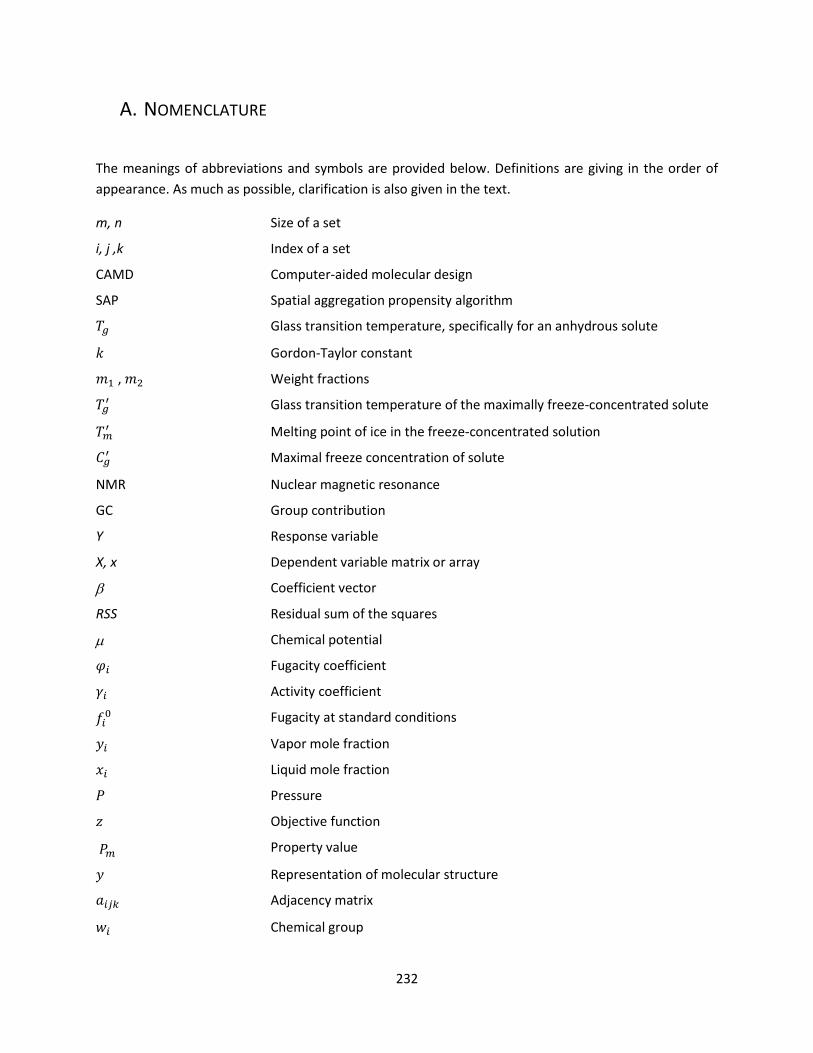
232
A. NOMENCLATURE
The meanings of abbreviations and symbols are provided below. Definitions are giving in the order of
appearance. As much as possible, clarification is also given in the text.
m, n Size of a set
i, j ,k Index of a set
CAMD Computer-aided molecular design
SAP Spatial aggregation propensity algorithm
Glass transition temperature, specifically for an anhydrous solute
Gordon-Taylor constant
, Weight fractions
Glass transition temperature of the maximally freeze-concentrated solute
Melting point of ice in the freeze-concentrated solution
Maximal freeze concentration of solute
NMR Nuclear magnetic resonance
GC Group contribution
Y Response variable
X, x Dependent variable matrix or array
Coefficient vector
RSS Residual sum of the squares
Chemical potential
Fugacity coefficient
Activity coefficient
Fugacity at standard conditions
Vapor mole fraction
Liquid mole fraction
Pressure
Objective function
Property value
Representation of molecular structure
Adjacency matrix
Chemical group

233
Structural constraint
Absorbance
Extinction coefficient
Concentration
Path length
Aggregation index
Optical density
Percent of protein monomer remaining after lyophilization
SEC Size exclusion chromatography
SDS-PAGE Sodium-dodecyl-sulfate polyacrylamide gel electrophoresis
pxrd Powder X-ray diffraction
Incident angle
l Wavelength
dhkl Characteristic vector defined by crystal geometry
<I> Intensity
Rate constant
HX-MS Hydrogen-deuterium exchange mass spectroscopy
Hildebrand solubility parameter
Td Thermal decomposition temperature
Kx Partition Coefficient, specificly for NDHD
EC50 Half maximal effective concentration
n Simple connectivity index of n-th order
n v Valence connectivity index of n-th order
Ns Number of subgraphs
i Vertex degree
iv Valence vertex degree
Z Atomic number
Zv Number of valence electrons
NH Number of connected hydrogen atoms
n Average simple connectivity index of n-th order
n v Average valence connectivity index of n-th order
a3vSA Sequence average amino acid aggregation propensity
nHS Number of aggregation hot spots

234
NnHS nHS normalized by number of residues in protein
AAT Area of aggregation profile above hot spot threshold
THSA Total area of aggregation profile comprising hot spots
TA Total area of aggregation profile
AATr AAT normalized by number of residues in protein
THSAr THSA normalized by number of residues in protein
Na4vSS Sliding window average of amino acid propensity values divided by number of amino acids in protein
Emin Minimum energy of PASTA pairings
Eavg Average energy of PASTA pairings
Lmax Average amino acid pair length of PASTA pairings
Lavg Maximum amino acid pair length of PASTA pairings
(E/L)min Minimum ratio of energy to length of PASTA pairings
(E/L)avg Average ratio of energy to length of PASTA pairings
# of Peaks Number of peaks in PASTA aggregation profile
Mallow's Cp statistic
p Number of parameters
Variance
LOOCV Leave-one-out cross-validation
PRESS Predicted residual sum of the square errors
Q2 Cross-validation coefficient
R2 Correlation coefficient
Sx Sensitivity
Percent average absolute deviation
Cohesive energy density
Molar volume
Enthalpy of vaporization
Volume fraction
Contribution of group
Rk Group volume parameters
Qk Surface area parameters
k Group residual activity coefficient
m Volume contribution parameter

235
Xm Group fraction parameter
nm Interaction parameter
anm Group interaction parameter
Error terms
( ) Binary variable declaring the existence of an alkyl chain
( ) , ( ) Binary variables declaring the existence of cation and anion
( ) Fitness of j-th member
⁄ Student’s t-test value
Dx Location of maximum driving force
Dy Value of maximum driving force
N Number of stages
NF Feed stage location
SF Scaling factor
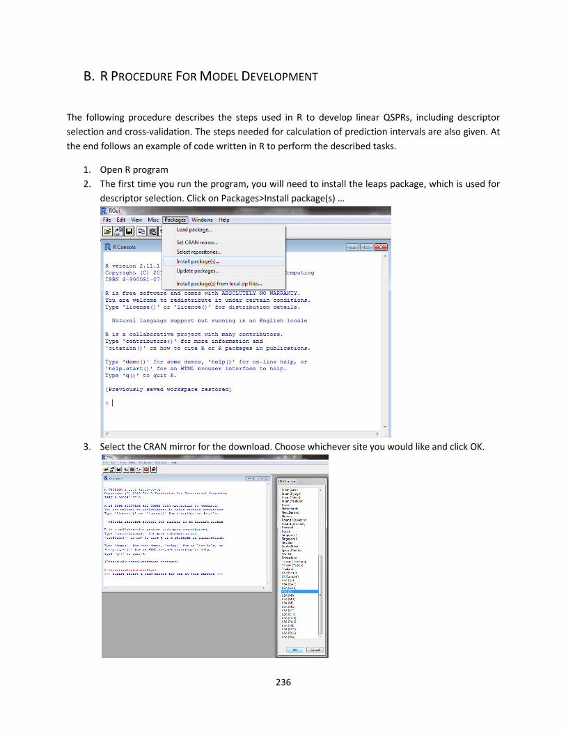
236
B. R PROCEDURE FOR MODEL DEVELOPMENT
The following procedure describes the steps used in R to develop linear QSPRs, including descriptor
selection and cross-validation. The steps needed for calculation of prediction intervals are also given. At
the end follows an example of code written in R to perform the described tasks.
1. Open R program
2. The first time you run the program, you will need to install the leaps package, which is used for
descriptor selection. Click on Pac ages>Install pac age(s) …
3. Select the CRAN mirror for the download. Choose whichever site you would like and click OK.
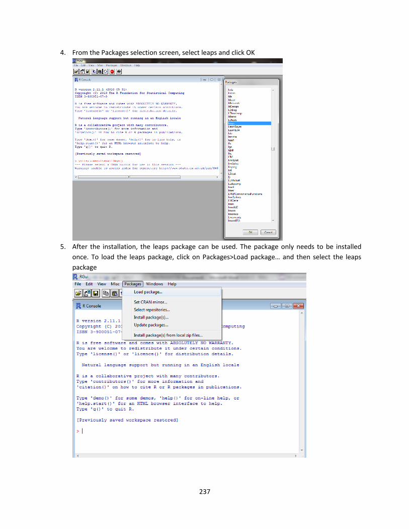
237
4. From the Packages selection screen, select leaps and click OK
5. After the installation, the leaps package can be used. The package only needs to be installed
once. To load the leaps pac age, clic on Pac ages> oad pac age… and then select the leaps
package

238
6. After the leaps package has loaded, the csv file containing the descriptor information and value
that is desired to be correlated should be loaded into R. The column headers in the csv file will
be used by R as names for the variable. Special characters are usually replaced by “X” and spaces
are replaced by “.”. To load the csv file, type the following command:
pick a name = read.csv(file.choose())
The name for the file is chosen by the user. A “Select file” window will pop up showing the user
directory. Navigate to the csv file desired and select the file. Click Open.
7. To attach the column headers to the variable names in R, type the following command
attach(pick a name)
Using whatever name you had chosen in step 6. To check that the file is loaded correctly and to
see the variable names that R is using, type
pick a name
Again using the name you had chosen in step 6. The csv file data will then display in R. Note the
variable names for each column, as they will be used to create the correlation later.
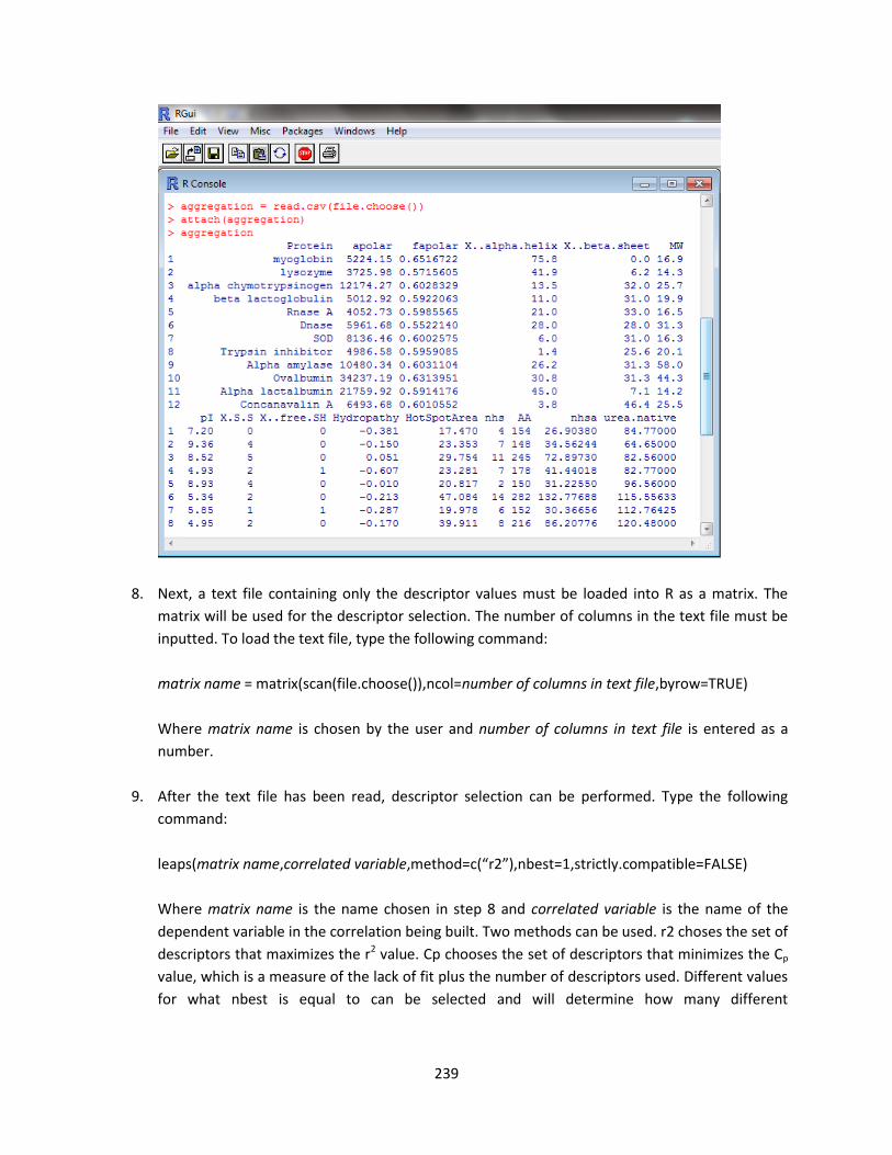
239
8. Next, a text file containing only the descriptor values must be loaded into R as a matrix. The
matrix will be used for the descriptor selection. The number of columns in the text file must be
inputted. To load the text file, type the following command:
matrix name = matrix(scan(file.choose()),ncol=number of columns in text file,byrow=TRUE)
Where matrix name is chosen by the user and number of columns in text file is entered as a
number.
9. After the text file has been read, descriptor selection can be performed. Type the following
command:
leaps(matrix name,correlated variable,method=c(“r ”),nbest=1,strictly.compatible=FALSE)
Where matrix name is the name chosen in step 8 and correlated variable is the name of the
dependent variable in the correlation being built. Two methods can be used. r2 choses the set of
descriptors that maximizes the r2 value. Cp chooses the set of descriptors that minimizes the Cp
value, which is a measure of the lack of fit plus the number of descriptors used. Different values
for what nbest is equal to can be selected and will determine how many different

240
correlations/models of each size (# of descriptors) will be reported. For example, nbest=3 would
report the three best models based upon the method chosen for each model size.
The output will display a matrix showing which descriptor was used for each correlation, as
indicated by TRUE or FALSE. The score given by the method selected will also be displayed.
10. Select a desired model/correlation for further analysis. Note the descriptors used in the model.
Build the correlation in R using the following command:
correlation name.lm <- lm(correlated variable~var1+var2 +…+varX)
Where correlation name is selected by the user, correlated variable is the dependent variable,
and var1 to varX are the descriptors selected using leaps. X denotes the size of the model (# of
descriptors).

241
11. The correlation information can be retrieved with the following command:
summary(correlation name.lm)
Where correlation name is the same as chosen in step 10.
12. To evaluate Q2, you must create a csv file containing only the selected descriptors and
correlated values. The variable names should remain the same to ensure that the correlation
can be used for cross-validation.
13. Cross-validation can then be performed using the following command:
User-definedName.CVlm <- CVlm(csv file name, correlationName.lm, m=number of folds, plotit=TRUE,
printit = TRUE)
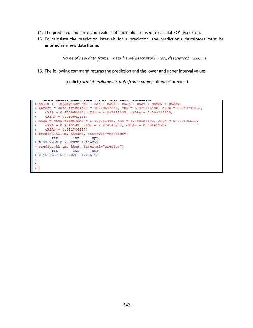
242
14. The predicted and correlation values of each fold are used to calculate Q2 (via excel).
15. To calculate the prediction intervals for a prediction, the prediction’s descriptors must be
entered as a new data frame:
Name of new data frame = data.frame(descriptor1 = xxx, descriptor2 = xxx, …)
16. The following command returns the prediction and the lower and upper interval value:
predict(correlationName.lm, data frame name, interval=”predict”)

243
An example code to complete the following steps is given below:
TIfields = read.csv(file.choose())
attach(TIfields)
TImatrix = matrix(scan(file.choose()),ncol=10,byrow=TRUE)
leaps(TImatrix,TI,method=c("Cp"),nbest=1,strictly.compatible=FALSE)
TI.lm <- lm(TI~cX4 + cX0A + cX1A + cX1v + cX3v + cX2Av + cX5Av)
summary(TI.lm)
TI.CVlm <- CVlm(TIfields, TI.lm, m=11, plotit=TRUE, printit = TRUE)
TItabu = data.frame(cX4 = 13.98383752, cX0A = 0.832184077,
cX1A = 0.603651, cX1v = 10.68623644, cX3v = 8.425098614,
cX2Av = 0.261058302, cX5Av = 0.057471174)
TIga = data.frame(cX4 = 7.903364617, cX0A = 0.846240068,
cX1A = 0.587963437, cX1v = 8.383716113, cX3v = 5.856908357,
cX2Av = 0.260155783, cX5Av = 0.067981002)
predict(TI.lm, TItabu, interval="predict")
predict(TI.lm, TIga, interval="predict")

244
C. POLYMER DESIGNER PROCEDURE
To open the Polymer Designer (pd2) executable, open the terminal in the pd2 Folder
Then in the terminal, type:
./pd2
In the program, you need to open a database. Clic “Open Database” and then select the database you
want to use.
To fill in the screen with info, clic on “select columns”. Some useful columns are Info>Name and
Descriptors> all the various connectivity indices. Then click Add Rows > Search and select the molecules
you want to be shown. This can be used to calculate connectivity indices.
To add new correlations, you must do the following
Close pd2
Open >src>tabu>dp_tabu_01.cpp
Scroll about ¾ of the way down and edit the correlations. Chii_# is the unweighted connectivity
index and xi_# is the weighted connectivity index.
Edit the cout information so your correlation values will be outputted
If you add any new variables, make sure they are declared in this file
o Then open >src>tabu>dp_tabu_01.hpp and define them there as well
Close both the .cpp and .hpp files
In the pd2 directory, delete the make file, pd2 executable file and pd2.pro file
Then follow the instructions for installing the program found in (Eslick 2009).

245
To run the tabu search:
Go to molecules>polymers>browse
Select a starting molecule (such as Tabu BisGMA) and click view
In the window that opens, go to the Toolbox and click on the graph tab. Then click Algorithm
Test and select Tabu test. The search results will display in the terminal.
To view and save a tabu search solution:
In pd2, go to Monomers>Browse>View and select anything
Go to the graph tab and select “import” then “yes”
Select your solution
Rearrange the atoms and bonds to better view your solution
Then close the molecule window
Go to Monomers>Browse>Add and your molecule should appear. Change the name and add a
description
To change the groups that will be used to build the tabu search solution:
Go to molecules>monomers>edit
Select a group from 09 to 18 to view. Only these are used by the program as building blocks.
In the molecule viewer, you can edit the bond and atoms. An Atomic # = 0 makes the atom a
connector. Every group must have at least one connector.
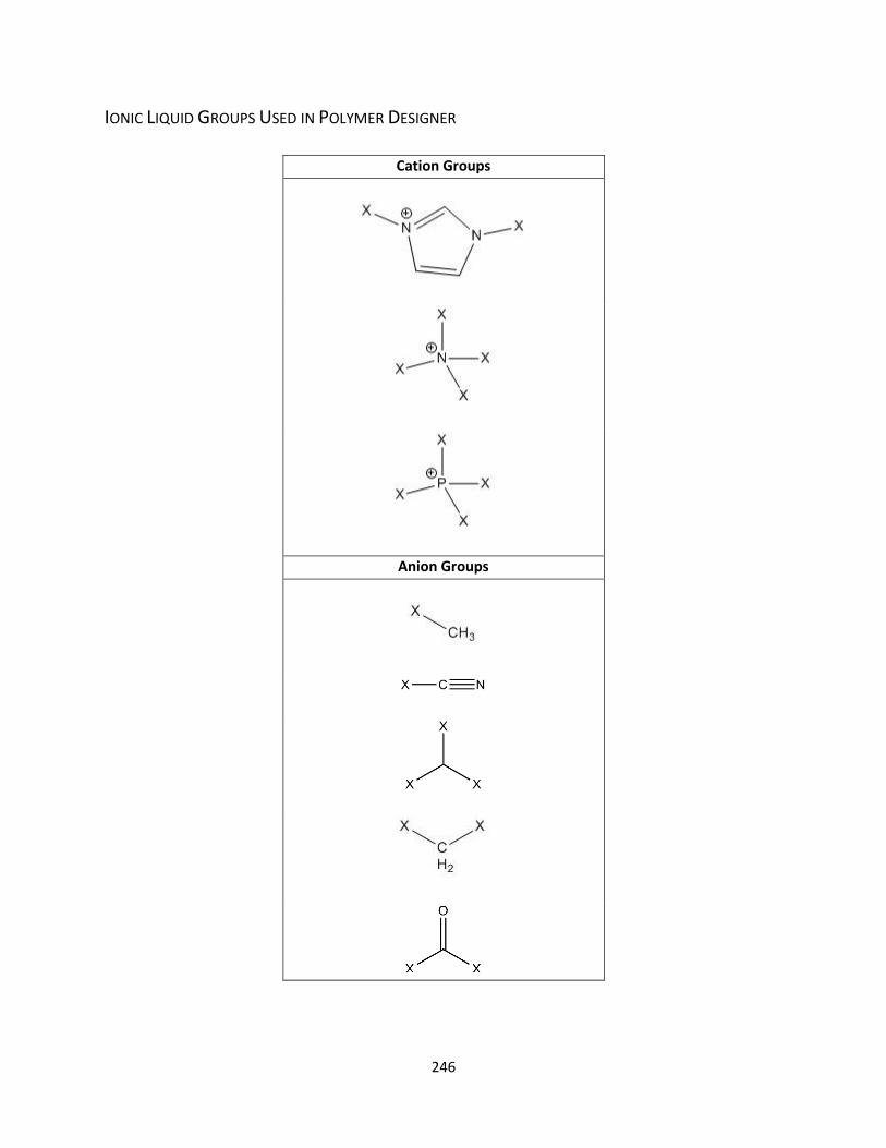
246
IONIC LIQUID GROUPS USED IN POLYMER DESIGNER
Cation Groups
Anion Groups
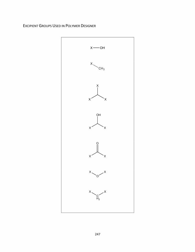
247
EXCIPIENT GROUPS USED IN POLYMER DESIGNER

248

249
D. CAMD EXCIPIENT DESIGNER SOURCE CODE
The following code is written in VBA and contains all the code used to design carbohydrate excipient
molecules for optimal %Monomer values. Modular programming was used with modules devoted to the
following tasks: Running searches and building molecules, calculating descriptors, calculating properties,
tabu search and genetic algorithm. In addition to the code provided here, data for each group is needed
in worksheets. Comments are indicated by an apostrophe (').
CAMD MODULE CODE Public n As Long, n_minusrings As Long Public m_max As Long Public Declare Function GetTickCount Lib "kernel32.dll" () As Long 'Returns time elapsed since startup in miliseconds Sub RunManyCAMD() Dim i As Long, j As Long, runs As Long Dim mol() As Long, mol_size As Long Dim Final_Obj As Double Dim t As Long runs = 100 Range("B2:O101").ClearContents For i = 1 To runs DoEvents 'Prevent not responding message t = GetTickCount Call CAMD(mol, Final_Obj) mol_size = UBound(mol) Cells(1 + i, 2) = i Cells(1 + i, 3) = Final_Obj Cells(1 + i, 4) = GetTickCount - t 'time elapsed while running code(and inserting i and obj values in excel - but that is negligible) Cells(1 + i, 5) = MW(mol) Cells(1 + i, 6) = HBD(mol) Cells(1 + i, 7) = HBA(mol) Cells(1 + i, 8) = Rings(mol) For j = 1 To mol_size Cells(1 + i, 8 + j) = mol(j) Next j Next i End Sub Sub CAMD(mol() As Long, Final_Obj As Double) 'argument mol() As Long, Final_Obj As Double

250
Dim m As Long, size As Long Dim i As Long, j As Long 'Dim mol() As Long, Final_Obj As Double 'arguments sometimes Dim del() As Long, delv() As Long, nH() As Long Dim AdjM() As Long, Chi(0 To 5) As Double, ChiV(0 To 5) As Double Dim Chi_Avg(0 To 5) As Double, ChiV_Avg(0 To 5) As Double m_max = 6 'maximum number of groups in molecule n = 89 ' number of groups n_minusrings = 9 'number of groups that are non-ring groups, also the first groups by order 'Create test solution -- For debugging 'Call InitialSolution(mol(), m) 'm = 5 'ReDim mol(1 To m) 'mol(1) = 1 'mol(2) = 37 'mol(3) = 3 'mol(4) = 71 'mol(5) = 1 'Create adjacency matrix and vectors to store del and delv values 'Call BuildMolecule(mol(), del(), delv(), nH(), AdjM(), m, size) 'Call GetConnectivity(del(), delv(), nH(), AdjM(), size, Chi(), ChiV(), Chi_Avg(), ChiV_Avg()) 'Final_Obj = obj(mol, Chi(), ChiV(), Chi_Avg(), ChiV_Avg()) Call RunTabu(mol(), m, del(), delv(), nH(), AdjM(), size, Chi(), ChiV(), Chi_Avg(), ChiV_Avg(), Final_Obj) 'Call RunGA(mol(), m, del(), delv(), nH(), AdjM(), size, Chi(), ChiV(), Chi_Avg(), ChiV_Avg(), Final_Obj) 'MsgBox "Best solution was MW = " & MW(mol) End Sub Sub InitialSolution(mol() As Long, m As Long) 'Build Random Initial Solution m = Int((m_max - 1 + 1) * Rnd + 1) ' groups in molecule ReDim mol(1 To m) 'Vector to store types of groups 'Randomly assign groups in the molecule For i = 1 To m If i > 1 Then If mol(i - 1) > n_minusriungs Then 'Make sure that you do not fuse two rings together mol(i) = Int((n_minusrings - 1 + 1) * Rnd + 1) 'Limits groups to non-ring groups Else

251
mol(i) = Int((n - 1 + 1) * Rnd + 1) 'Entire selection of groups available End If Else mol(i) = Int((n - 1 + 1) * Rnd + 1) 'Entire selection of groups available for first group added End If Next i End Sub Sub BuildMolecule(mol() As Long, del() As Long, delv() As Long, nH() As Long, AdjM() As Long, m As Long, size As Long) 'Creates adjacency matrix, del and delv values for groups selected Dim i As Long, j As Long, k As Long, jstart As Long, kstart As Long, jlag As Long Dim terminal As Long 'Clear old Adjacency Matrix Erase AdjM() 'Always will have two terminals size = 2 'Calculate number of non-hydrogen atoms in the molecule For i = 1 To m size = size + atoms(mol(i)) Next i 'Size adjacency matrix and del/delv vectors to proper size ReDim AdjM(1 To size, 1 To size) ReDim del(1 To size) ReDim delv(1 To size) ReDim nH(1 To size) 'Set terminals values for del and delv ' This sets both terminals to -OH (hydroxyl) groups del(1) = 8 del(size) = 8 delv(1) = 6 delv(size) = 6 nH(1) = 1 nH(size) = 1 'Set starting indices jstart = 2 'used to store starting node for group being added to molecule kstart = jstart jlag = 1 'used to store terminal node from previous group added to molecule For i = 1 To m

252
AdjM(jlag, jstart) = 1 'Connects starting node from new group with terminal node from previous group AdjM(jstart, jlag) = 1 'Obtains del/delv values and connectivity for group selected by accessing workbook For j = jstart To jstart + atoms(mol(i)) - 1 del(j) = Worksheets(Name(mol(i))).Cells(3 + (j - jstart), 2).Value delv(j) = Worksheets(Name(mol(i))).Cells(3 + (j - jstart), 3).Value nH(j) = Worksheets(Name(mol(i))).Cells(3 + (j - jstart), 4).Value For k = kstart To kstart + atoms(mol(i)) - 1 AdjM(j, k) = Worksheets(Name(mol(i))).Cells(2 + (j - jstart), 6 + (k - jstart)).Value Next k Next j 'Finds terminal node for group added and node for next group to be added jlag = terminus(mol(i), jstart) jstart = jstart + atoms(mol(i)) kstart = kstart + atoms(mol(i)) Next i AdjM(jlag, size) = 1 'Connects terminal node from new group with terminal AdjM(size, jlag) = 1 End Sub Function atoms(molecule_group As Long) As Long 'Assigns number of atoms in group selected Select Case molecule_group Case Is = 1 atoms = 1 Case 2 To 3 atoms = 2 Case Is = 4 atoms = 1 Case Is = 5 atoms = 2 Case 6 To 9 atoms = 5 Case 10 To 25 atoms = 7 Case 26 To 41 atoms = 9 Case 42 To 57

253
atoms = 8 Case 58 To 89 atoms = 9 End Select End Function Function Name(molecule_group As Long) As String 'Assigns name to group selected Select Case molecule_group Case Is = 1 Name = "Group1" Case Is = 2 Name = "Group2a" Case Is = 3 Name = "Group2b" Case Is = 4 Name = "Group3" Case Is = 5 Name = "Group4" Case Is = 6 Name = "Group5a" Case Is = 7 Name = "Group5b" Case Is = 8 Name = "Group5c" Case Is = 9 Name = "Group5d" Case Is = 10 Name = "Group6a" Case Is = 11 Name = "Group6b" Case Is = 12 Name = "Group6c" Case Is = 13 Name = "Group6d" Case Is = 14 Name = "Group6e" Case Is = 15 Name = "Group6f" Case Is = 16 Name = "Group6g" Case Is = 17 Name = "Group6h" Case Is = 18 Name = "Group6i" Case Is = 19

254
Name = "Group6j" Case Is = 20 Name = "Group6k" Case Is = 21 Name = "Group6l" Case Is = 22 Name = "Group6m" Case Is = 23 Name = "Group6n" Case Is = 24 Name = "Group6o" Case Is = 25 Name = "Group6p" Case Is = 26 Name = "Group7a" Case Is = 27 Name = "Group7b" Case Is = 28 Name = "Group7c" Case Is = 29 Name = "Group7d" Case Is = 30 Name = "Group7e" Case Is = 31 Name = "Group7f" Case Is = 32 Name = "Group7g" Case Is = 33 Name = "Group7h" Case Is = 34 Name = "Group7i" Case Is = 35 Name = "Group7j" Case Is = 36 Name = "Group7k" Case Is = 37 Name = "Group7l" Case Is = 38 Name = "Group7m" Case Is = 39 Name = "Group7n" Case Is = 40 Name = "Group7o" Case Is = 41 Name = "Group7p" Case Is = 42 Name = "Group8a" Case Is = 43

255
Name = "Group8b" Case Is = 44 Name = "Group8c" Case Is = 45 Name = "Group8d" Case Is = 46 Name = "Group8e" Case Is = 47 Name = "Group8f" Case Is = 48 Name = "Group8g" Case Is = 49 Name = "Group8h" Case Is = 50 Name = "Group8i" Case Is = 51 Name = "Group8j" Case Is = 52 Name = "Group8k" Case Is = 53 Name = "Group8l" Case Is = 54 Name = "Group8m" Case Is = 55 Name = "Group8n" Case Is = 56 Name = "Group8o" Case Is = 57 Name = "Group8p" Case Is = 58 Name = "Group9a" Case Is = 59 Name = "Group9b" Case Is = 60 Name = "Group9c" Case Is = 61 Name = "Group9d" Case Is = 62 Name = "Group9e" Case Is = 63 Name = "Group9f" Case Is = 64 Name = "Group9g" Case Is = 65 Name = "Group9h" Case Is = 66 Name = "Group9i" Case Is = 67

256
Name = "Group9j" Case Is = 68 Name = "Group9k" Case Is = 69 Name = "Group9l" Case Is = 70 Name = "Group9m" Case Is = 71 Name = "Group9n" Case Is = 72 Name = "Group9o" Case Is = 73 Name = "Group9p" Case Is = 74 Name = "Group9q" Case Is = 75 Name = "Group9r" Case Is = 76 Name = "Group9s" Case Is = 77 Name = "Group9t" Case Is = 78 Name = "Group9u" Case Is = 79 Name = "Group9v" Case Is = 80 Name = "Group9w" Case Is = 81 Name = "Group9x" Case Is = 82 Name = "Group9y" Case Is = 83 Name = "Group9z" Case Is = 84 Name = "Group9aa" Case Is = 85 Name = "Group9ab" Case Is = 86 Name = "Group9ac" Case Is = 87 Name = "Group9ad" Case Is = 88 Name = "Group9ae" Case Is = 89 Name = "Group9af" End Select End Function

257
Function terminus(molecule_group As Long, jstart As Long) As String 'Finds right hand side terminal atom Select Case molecule_group Case 1 To 9 terminus = jstart Case 10 To 89 terminus = jstart + atoms(molecule_group) - 1 'Different atom joins to next group than prior group End Select End Function
PROPERTY MODULE CODE Function MW(mol) As Double Dim sum As Long, size As Long Dim i As Long m = UBound(mol) sum = 34 For i = 1 To m Select Case mol(i) Case Is = 1 sum = sum + 14 Case 2 To 3 sum = sum + 30 Case Is = 4 sum = sum + 16 Case Is = 5 sum = sum + 28 Case 6 To 9 sum = sum + 3 * 12 + 2 * 16 + 6 * 1 Case 10 To 25 sum = sum + 4 * 12 + 3 * 16 + 6 Case 26 To 41 sum = sum + 5 * 12 + 4 * 16 + 8 Case 42 To 57 sum = sum + 5 * 12 + 3 * 16 + 8 Case 58 To 89 sum = sum + 5 * 12 + 4 * 16 + 8 End Select Next i MW = sum

258
End Function Function HBD(mol) As Double Dim sum As Long, size As Long Dim i As Long m = UBound(mol) sum = 2 For i = 1 To m Select Case mol(i) Case Is = 1 sum = sum + 0 Case 2 To 3 sum = sum + 1 Case Is = 4 sum = sum + 0 Case Is = 5 sum = sum + 0 Case 6 To 9 sum = sum + 2 Case 10 To 25 sum = sum + 2 Case 26 To 41 sum = sum + 3 Case 42 To 57 sum = sum + 2 Case 58 To 89 sum = sum + 3 End Select Next i HBD = sum End Function Function HBA(mol) As Double Dim sum As Long, size As Long Dim i As Long m = UBound(mol) sum = 2 For i = 1 To m Select Case mol(i) Case Is = 1
259
sum = sum + 0 Case 2 To 3 sum = sum + 1 Case Is = 4 sum = sum + 1 Case Is = 5 sum = sum + 1 Case 6 To 9 sum = sum + 2 Case 10 To 25 sum = sum + 3 Case 26 To 41 sum = sum + 4 Case 42 To 57 sum = sum + 3 Case 58 To 89 sum = sum + 4 End Select Next i HBA = sum End Function Function Rings(mol) As Double Dim sum As Long, size As Long Dim i As Long m = UBound(mol) sum = 0 For i = 1 To m Select Case mol(i) Case Is = 1 sum = sum + 0 Case 2 To 3 sum = sum + 0 Case Is = 4 sum = sum + 0 Case Is = 5 sum = sum + 0 Case 6 To 9 sum = sum + 0 Case 10 To 25 sum = sum + 1 Case 26 To 41 sum = sum + 1

260
Case 42 To 57 sum = sum + 1 Case 58 To 89 sum = sum + 1 End Select Next i Rings = sum End Function Function obj(mol, Chi() As Double, ChiV() As Double, Chi_Avg() As Double, ChiV_Avg() As Double) As Double Dim Prop_MW As Double, Prop_RNA As Double, Prop_BSA As Double, Prop_AA As Double, Prop_Ova As Double, Prop_TI As Double Dim Target_MW As Double, Target1 As Double, Prop_All As Double Dim ASA As Double, ahelix As Double, bsheet As Double, MW_prot As Double, Tm As Double 'Design Targets Target_MW = 342 Target1 = 1# '1.64092082073789 'Target2 = 1# '-0.99286646595339 'Protein Properties -- Read from user at later date ASA = 4052 ahelix = 21 bsheet = 33 MW_prot = 16.5 Tm = 62.5 Penalty = 0 Prop_MW = MW(mol) Prop_RNA = 12.271 + 0.0637 * Chi(1) + 0.5761 * Chi(3) - 0.1392 * Chi(5) - 18.2244 * Chi_Avg(0) + 3.9332 * Chi_Avg(2) + _ 6.0029 * Chi_Avg(5) + 0.6086 * ChiV(1) - 2.5101 * ChiV(2) + 3.5378 * ChiV(4) - 3.1432 * ChiV(5) + _ 36.8323 * ChiV_Avg(2) - 44.3452 * ChiV_Avg(3) - 19.6284 * ChiV_Avg(4) + 13.1564 * ChiV_Avg(5) Prop_BSA = 5.9445 - 0.279 * Chi(3) - 0.3754 * Chi(5) - 10.0317 * Chi_Avg(0) + 7.5983 * Chi_Avg(1) - 16.2788 * Chi_Avg(4) + 23.4753 * Chi_Avg(5) + _ 0.2149 * ChiV(0) - 0.7594 * ChiV(1) - 0.1974 * ChiV(2) + 2.2207 * ChiV(3) - 0.7265 * ChiV(5) + _ 8.4658 * ChiV_Avg(2) - 21.0254 * ChiV_Avg(3) Prop_AA = 0.6937 - 0.3134 * Chi(3) - 0.1253 * Chi(5) + 1.6912 * Chi_Avg(0) + 5.1275 * Chi_Avg(2) + _ 0.8448 * ChiV(3) - 2.3518 * ChiV_Avg(0) - 7.97 * ChiV_Avg(2) Prop_Ova = 1.1102 - 0.0514 * Chi(2) + 0.5165 * Chi(4) + 1.0148 * Chi_Avg(2) - 7.149 * Chi_Avg(5) - _ 1.0949 * ChiV(4) - 0.4271 * ChiV_Avg(0) - 1.4052 * ChiV_Avg(4) + 16.5246 * ChiV_Avg(5)
261
Prop_TI = -6.786 + 0.1362 * Chi(4) + 13.9898 * Chi_Avg(0) - 11.5258 * Chi_Avg(1) + 0.0346 * ChiV(1) - _ 0.2911 * ChiV(3) + 16.7938 * ChiV_Avg(2) - 19.2179 * ChiV_Avg(5) Prop_All = 0.0000251 * (-2.43 * Chi(0) + 6.52 * Chi(1) - 3.12 * Chi(2) - 94.32 * Chi_Avg(1) + 74.04 * Chi_Avg(2)) * _ (0.029 * ASA + 19.35 * ahelix - 60.34 * bsheet - 71.54 * MW_prot + 66.38 * Tm) 'Penalty Function For i = 1 To UBound(mol) If mol(1) = 4 Or mol(UBound(mol)) = 4 Then 'Add penalty for O-OH bond Penalty = 1000 Exit For End If If i > 1 Then If mol(i - 1) > n_minusrings And mol(i) > n_minusrings Then 'Add penalty if two rings are fused together Penalty = 1000 Exit For ElseIf mol(i - 1) = 4 And mol(i) = 4 Then 'Add penalty for O-O bond Penalty = 1000 Exit For End If End If Next i obj = Abs(Prop_MW - Target_MW) / Abs(Target_MW) ' + Penalty End Function Function fitness(mol) As Double Target_MW = 148 Lower_MW = 0 Higher_MW = 296 alpha = 0.001 fitness = Exp(-alpha * (MW(mol) - Target_MW) ^ 2 / (Higher_MW - Lower_MW) ^ 2) End Function

262
Function RNAmonomer(groups As Range) As Double Dim mol() As Long, m As Long, size As Long, i As Long Dim del() As Long, delv() As Long, nH() As Long Dim AdjM() As Long, Chi(0 To 5) As Double, ChiV(0 To 5) As Double Dim Chi_Avg(0 To 5) As Double, ChiV_Avg(0 To 5) As Double m = groups.Count ReDim mol(1 To m) For i = 1 To m mol(i) = groups(i).Value Next i Call BuildMolecule(mol(), del(), delv(), nH(), AdjM(), m, size) Call GetConnectivity(del(), delv(), nH(), AdjM(), size, Chi(), ChiV(), Chi_Avg(), ChiV_Avg()) RNAmonomer = 12.271 + 0.0637 * Chi(1) + 0.5761 * Chi(3) - 0.1392 * Chi(5) - 18.2244 * Chi_Avg(0) + 3.9332 * Chi_Avg(2) + _ 6.0029 * Chi_Avg(5) + 0.6086 * ChiV(1) - 2.5101 * ChiV(2) + 3.5378 * ChiV(4) - 3.1432 * ChiV(5) + _ 36.8323 * ChiV_Avg(2) - 44.3452 * ChiV_Avg(3) - 19.6284 * ChiV_Avg(4) + 13.1564 * ChiV_Avg(5) End Function Function BSAmonomer(groups As Range) As Double Dim mol() As Long, m As Long, size As Long, i As Long Dim del() As Long, delv() As Long, nH() As Long Dim AdjM() As Long, Chi(0 To 5) As Double, ChiV(0 To 5) As Double Dim Chi_Avg(0 To 5) As Double, ChiV_Avg(0 To 5) As Double m = groups.Count ReDim mol(1 To m) For i = 1 To m mol(i) = groups(i).Value Next i Call BuildMolecule(mol(), del(), delv(), nH(), AdjM(), m, size) Call GetConnectivity(del(), delv(), nH(), AdjM(), size, Chi(), ChiV(), Chi_Avg(), ChiV_Avg()) BSAmonomer = 5.9445 - 0.279 * Chi(3) - 0.3754 * Chi(5) - 10.0317 * Chi_Avg(0) + 7.5983 * Chi_Avg(1) - 16.2788 * Chi_Avg(4) + 23.4753 * Chi_Avg(5) + _ 0.2149 * ChiV(0) - 0.7594 * ChiV(1) - 0.1974 * ChiV(2) + 2.2207 * ChiV(3) - 0.7265 * ChiV(5) + _ 8.4658 * ChiV_Avg(2) - 21.0254 * ChiV_Avg(3) End Function Function AAmonomer(groups As Range) As Double
263
Dim mol() As Long, m As Long, size As Long, i As Long Dim del() As Long, delv() As Long, nH() As Long Dim AdjM() As Long, Chi(0 To 5) As Double, ChiV(0 To 5) As Double Dim Chi_Avg(0 To 5) As Double, ChiV_Avg(0 To 5) As Double m = groups.Count ReDim mol(1 To m) For i = 1 To m mol(i) = groups(i).Value Next i Call BuildMolecule(mol(), del(), delv(), nH(), AdjM(), m, size) Call GetConnectivity(del(), delv(), nH(), AdjM(), size, Chi(), ChiV(), Chi_Avg(), ChiV_Avg()) AAmonomer = 0.6937 - 0.3134 * Chi(3) - 0.1253 * Chi(5) + 1.6912 * Chi_Avg(0) + 5.1275 * Chi_Avg(2) + _ 0.8448 * ChiV(3) - 2.3518 * ChiV_Avg(0) - 7.97 * ChiV_Avg(2) End Function Function OVAmonomer(groups As Range) As Double Dim mol() As Long, m As Long, size As Long, i As Long Dim del() As Long, delv() As Long, nH() As Long Dim AdjM() As Long, Chi(0 To 5) As Double, ChiV(0 To 5) As Double Dim Chi_Avg(0 To 5) As Double, ChiV_Avg(0 To 5) As Double m = groups.Count ReDim mol(1 To m) For i = 1 To m mol(i) = groups(i).Value Next i Call BuildMolecule(mol(), del(), delv(), nH(), AdjM(), m, size) Call GetConnectivity(del(), delv(), nH(), AdjM(), size, Chi(), ChiV(), Chi_Avg(), ChiV_Avg()) OVAmonomer = 1.1102 - 0.0514 * Chi(2) + 0.5165 * Chi(4) + 1.0148 * Chi_Avg(2) - 7.149 * Chi_Avg(5) - _ 1.0949 * ChiV(4) - 0.4271 * ChiV_Avg(0) - 1.4052 * ChiV_Avg(4) + 16.5246 * ChiV_Avg(5) End Function Function TImonomer(groups As Range) As Double Dim mol() As Long, m As Long, size As Long, i As Long Dim del() As Long, delv() As Long, nH() As Long Dim AdjM() As Long, Chi(0 To 5) As Double, ChiV(0 To 5) As Double Dim Chi_Avg(0 To 5) As Double, ChiV_Avg(0 To 5) As Double m = groups.Count

264
ReDim mol(1 To m) For i = 1 To m mol(i) = groups(i).Value Next i Call BuildMolecule(mol(), del(), delv(), nH(), AdjM(), m, size) Call GetConnectivity(del(), delv(), nH(), AdjM(), size, Chi(), ChiV(), Chi_Avg(), ChiV_Avg()) TImonomer = -6.786 + 0.1362 * Chi(4) + 13.9898 * Chi_Avg(0) - 11.5258 * Chi_Avg(1) + 0.0346 * ChiV(1) - _ 0.2911 * ChiV(3) + 16.7938 * ChiV_Avg(2) - 19.2179 * ChiV_Avg(5) End Function Sub ReturnCI() Dim mol() As Long, m As Long, size As Long, i As Long, groups As Range Dim del() As Long, delv() As Long, nH() As Long Dim AdjM() As Long, Chi(0 To 5) As Double, ChiV(0 To 5) As Double Dim Chi_Avg(0 To 5) As Double, ChiV_Avg(0 To 5) As Double Set groups = Application.InputBox("Select groups", Type:=8) m = groups.Count ReDim mol(1 To m) For i = 1 To m mol(i) = groups(i).Value Next i Call BuildMolecule(mol(), del(), delv(), nH(), AdjM(), m, size) Call GetConnectivity(del(), delv(), nH(), AdjM(), size, Chi(), ChiV(), Chi_Avg(), ChiV_Avg()) For i = 0 To 5 ActiveCell.Offset(0, i) = Chi(i) ActiveCell.Offset(1, i) = ChiV(i) ActiveCell.Offset(2, i) = Chi_Avg(i) ActiveCell.Offset(3, i) = ChiV_Avg(i) Next i End Sub
CONNECTIVITY INDICES CALCULATOR CODE Option Explicit Sub GetConnectivity(del() As Long, delv() As Long, nH() As Long, AdjM() As Long, m As Long, Chi() As Double, ChiV() As Double, _ Chi_Avg() As Double, ChiV_Avg() As Double) Dim i As Long, j As Long, k As Long, edgecount As Long

265
Dim path2count() As Double, path2sum As Double, p As Long Dim path3count() As Double, path3sum As Double, i3 As Long Dim path4count() As Double, path4sum As Double, i4 As Long Dim path5count() As Double, path5sum As Double, i5 As Long Dim av() As Double, avv() As Double, e() As Double, ev() As Double 'Clear old results Erase Chi() Erase ChiV() Erase Chi_Avg() Erase ChiV_Avg() 'ReDim all relevant arrays ReDim av(1 To m) 'Array for vertex degrees ReDim avv(1 To m) 'Array for valence vertex degrees ReDim path2count(1 To m, 1 To m, 1 To m) 'Array for storing existence of 2-length paths ReDim path3count(1 To m, 1 To m) 'Array for storing existence of 3-length paths ReDim path4count(1 To m, 1 To m) 'Array for storing existence of 4-length paths ReDim path5count(1 To m, 1 To m) 'Array for storing existence of 5-length paths 'Calculate valence vertex degrees For i = 1 To m avv(i) = (delv(i) - nH(i)) / (del(i) - delv(i) - 1) + AdjM(i, i) Next i 'Calculate vertex degrees and X0 and X0v For i = 1 To m For j = 1 To m av(i) = AdjM(i, j) + av(i) Next j If av(i) = 0 Then MsgBox "Disconnected Atom", , "Error" Exit Sub End If Chi(0) = Chi(0) + 1 / (av(i) ^ 0.5) ChiV(0) = ChiV(0) + 1 / (avv(i) ^ 0.5) Next i 'Count number of edges For i = 2 To m For j = 1 To i - 1 If AdjM(i, j) > 0 Then edgecount = edgecount + 1 Next j Next i 'Dimension array to size of number of edges ReDim e(1 To edgecount)

266
ReDim ev(1 To edgecount) 'Calculate edge values and X1 and X1v k = 1 For i = 2 To m For j = 1 To i - 1 If AdjM(i, j) > 0 Then e(k) = av(i) * av(j) ev(k) = avv(i) * avv(j) Chi(1) = Chi(1) + 1 / (e(k) ^ 0.5) ChiV(1) = ChiV(1) + 1 / (ev(k) ^ 0.5) k = k + 1 End If Next j Next i 'Records existence of paths of length 2 For i = 1 To m For j = 1 To m If j <> i Then If AdjM(i, j) > 0 Then For k = 1 To m If k <> j And k <> i Then If AdjM(j, k) > 0 Then If path2count(k, j, i) > 0 Then path2count(i, j, k) = 0 Else path2count(i, j, k) = 1 End If End If End If Next k End If End If Next j Next i 'Calculate X2 and X2v For i = 1 To m For j = 1 To m For k = 1 To m path2sum = path2sum + path2count(i, j, k) 'Count the number of paths of length 2 - Mainly for debugging purposes If path2count(i, j, k) > 0 Then Chi(2) = Chi(2) + 1 / ((av(i) * av(j) * av(k)) ^ 0.5) ChiV(2) = ChiV(2) + 1 / ((avv(i) * avv(j) * avv(k)) ^ 0.5) End If Next k

267
Next j Next i 'Check for paths of length 3, 4 and 5 For i = 1 To m For j = 1 To m If j <> i Then If AdjM(i, j) > 0 Then For k = 1 To m If k <> j And k <> i Then If AdjM(j, k) > 0 Then For i3 = 1 To m If i3 <> k And i3 <> j And i3 <> i Then If AdjM(k, i3) > 0 Then If path3count(i3, i) > 0 Then path3count(i, i3) = 0 ' Avoids double counting paths Else path3count(i, i3) = 1 path3sum = path3sum + 1 Chi(3) = Chi(3) + 1 / ((av(i) * av(j) * av(k) * av(i3)) ^ 0.5) ChiV(3) = ChiV(3) + 1 / ((avv(i) * avv(j) * avv(k) * avv(i3)) ^ 0.5) End If For i4 = 1 To m If i4 <> i3 And i4 <> k And i4 <> j And i4 <> i Then If AdjM(i3, i4) > 0 Then If path4count(i4, i) > 0 Then path4count(i, i4) = 0 Else path4count(i, i4) = 1 path4sum = path4sum + 1 Chi(4) = Chi(4) + 1 / ((av(i) * av(j) * av(k) * av(i3) * av(i4)) ^ 0.5) ChiV(4) = ChiV(4) + 1 / ((avv(i) * avv(j) * avv(k) * avv(i3) * avv(i4)) ^ 0.5) End If For i5 = 1 To m If i5 <> i3 And i5 <> k And i5 <> j And i5 <> i4 And i5 <> i Then 'i5 cannot equal i even if there is a five atom ring -- Paths not walks! If AdjM(i4, i5) > 0 Then If path5count(i5, i) > 0 Then path5count(i, i5) = 0 Else path5count(i, i5) = 1 path5sum = path5sum + 1 Chi(5) = Chi(5) + 1 / ((av(i) * av(j) * av(k) * av(i3) * av(i4) * av(i5)) ^ 0.5) ChiV(5) = ChiV(5) + 1 / ((avv(i) * avv(j) * avv(k) * avv(i3) * avv(i4) * avv(i5)) ^ 0.5) End If End If

268
End If Next i5 End If End If Next i4 End If End If Next i3 End If End If Next k End If End If Next j Next i 'Calculate XAs 'Molecule guarenteed to have path of length 2, but need to check if any path length > 2 to avoid overflow Chi_Avg(0) = Chi(0) / m Chi_Avg(1) = Chi(1) / edgecount Chi_Avg(2) = Chi(2) / path2sum If path3sum <> 0 Then Chi_Avg(3) = Chi(3) / path3sum Else Chi_Avg(3) = 0 End If If path4sum <> 0 Then Chi_Avg(4) = Chi(4) / path4sum Else Chi_Avg(4) = 0 End If If path5sum <> 0 Then Chi_Avg(5) = Chi(5) / path5sum Else Chi_Avg(5) = 0 End If ChiV_Avg(0) = ChiV(0) / m ChiV_Avg(1) = ChiV(1) / edgecount ChiV_Avg(2) = ChiV(2) / path2sum If path3sum <> 0 Then ChiV_Avg(3) = ChiV(3) / path3sum Else ChiV_Avg(3) = 0 End If If path4sum <> 0 Then
269
ChiV_Avg(4) = ChiV(4) / path4sum Else ChiV_Avg(4) = 0 End If If path5sum <> 0 Then ChiV_Avg(5) = ChiV(5) / path5sum Else ChiV_Avg(5) = 0 End If End Sub
TABU SEARCH CODE ption Explicit Sub RunTabu(mol() As Long, m As Long, del() As Long, delv() As Long, nH() As Long, AdjM() As Long, size As Long, _ Chi() As Double, ChiV() As Double, Chi_Avg() As Double, ChiV_Avg() As Double, Final_Obj As Double) Dim moves As Long, max_moves As Long, TabuCriterion As Double, Stop_Criterion As Double Dim imax As Long, List_size As Long, Tabu_list() As Variant, Tabu_count As Long Dim Neighbors() As Molecule, p() As Double Dim Best_sol() As Long, Current_sol() As Long, Neighbor_sol() As Long Dim Best_obj As Double, Current_obj As Double, Neighbor_obj As Double Dim Neighbors_Chi(0 To 5) As Double, Neighbors_ChiV(0 To 5) As Double, Neighbors_Chi_Avg(0 To 5) As Double, Neighbors_ChiV_Avg(0 To 5) As Double Dim Current_Chi(0 To 5) As Double, Current_ChiV(0 To 5) As Double, Current_Chi_Avg(0 To 5) As Double, Current_ChiV_Avg(0 To 5) As Double Dim Best_Chi(0 To 5) As Double, Best_ChiV(0 To 5) As Double, Best_Chi_Avg(0 To 5) As Double, Best_ChiV_Avg(0 To 5) As Double Dim i As Long, j As Long, k As Long, iter As Long imax = 100# 'Max number of non-improving iterations List_size = 15# 'Size of tabu list ReDim Tabu_list(1 To List_size, 1 To 2) 'Set length of tabu list. '1st column is for molecule groups. 2nd column is for Chi0 values used in tabu check. max_moves = 4# 'maximum number of moves to create neighbors TabuCriterion = 0.2 'Criterion for making solution Tabu Stop_Criterion = 0# 'Criterion for objective function being good enough to stop 'Create random initial solution Call InitialSolution(mol(), m) 'Initial solution set as best solution and current solution Best_sol = mol 'Stores structure

270
Current_sol = mol 'Stores structure Call BuildMolecule(mol, del(), delv(), nH(), AdjM(), m, size) Call GetConnectivity(del(), delv(), nH(), AdjM(), size, Chi(), ChiV(), Chi_Avg(), ChiV_Avg()) For k = 0 To 5 Current_Chi(k) = Chi(k) Current_ChiV(k) = ChiV(k) Current_Chi_Avg(k) = Chi_Avg(k) Current_ChiV_Avg(k) = ChiV_Avg(k) Next k Best_obj = obj(mol, Chi(), ChiV(), Chi_Avg(), ChiV_Avg()) 'Stores objective value Tabu_list(1, 1) = mol 'Put initial solution into tabu list Tabu_list(1, 2) = Chi(0) 'Stores Chi0 for tabu solution 'Tabu Search Do DoEvents 'Prevent not responding moves = Int((max_moves - 1 + 1) * Rnd + 1) 'Max number of neighbors evaluated ReDim Neighbors(1 To moves) 'initialize array for storing neighbors ReDim p(1 To moves) 'initialize array for storing objective function values of neighbors 'Create list of neighbors and neighbor properties For j = 1 To moves Neighbors(j).mol = Make_Neighbor(Current_sol, m) Call BuildMolecule(Neighbors(j).mol, del(), delv(), nH(), AdjM(), m, size) Call GetConnectivity(del(), delv(), nH(), AdjM(), size, Chi(), ChiV(), Chi_Avg(), ChiV_Avg()) For k = 0 To 5 Neighbors(j).Chi(k) = Chi(k) Neighbors(j).ChiV(k) = ChiV(k) Neighbors(j).Chi_Avg(k) = Chi_Avg(k) Neighbors(j).ChiV_Avg(k) = ChiV_Avg(k) Next k p(j) = obj(Neighbors(j).mol(), Chi(), ChiV(), Chi_Avg(), ChiV_Avg()) Next j Neighbor_obj = p(1) 'Arbitrarily sets first neighbor as best objective function value 'Determine best non-tabu neighbor For j = 1 To moves Tabu_count = 0 'Initialize If p(j) <= Neighbor_obj Then 'If objective function of neighbor is better than previous best, replace For i = 1 To List_size 'Check against each member of tabu list If Abs(Neighbors(j).Chi(0) - Tabu_list(i, 2)) > TabuCriterion Then 'Tabu Check Tabu_count = 0 'Solution is not Tabu yet... Else Tabu_count = 1 'Solution is Tabu. Quit checking against Tabu List.

271
Exit For End If Next i If Tabu_count = 0 Then 'Check to see if solution is tabu. If not, assign solution to surrent solution. Neighbor_sol = Neighbors(j).mol Neighbor_obj = p(j) For k = 0 To 5 Neighbors_Chi(k) = Neighbors(j).Chi(k) Neighbors_ChiV(k) = Neighbors(j).ChiV(k) Neighbors_Chi_Avg(k) = Neighbors(j).Chi_Avg(k) Neighbors_ChiV_Avg(k) = Neighbors(j).ChiV_Avg(k) Next k ElseIf p(j) <= Best_obj Then 'Override Tabu Criterion if solution is best yet encountered Neighbor_sol = Neighbors(j).mol Neighbor_obj = p(j) For k = 0 To 5 Neighbors_Chi(k) = Neighbors(j).Chi(k) Neighbors_ChiV(k) = Neighbors(j).ChiV(k) Neighbors_Chi_Avg(k) = Neighbors(j).Chi_Avg(k) Neighbors_ChiV_Avg(k) = Neighbors(j).ChiV_Avg(k) Next k If p(j) <= Stop_Criterion Then 'Stop search if you have found best possible/allowable solution Neighbor_sol = Best_sol Neighbor_obj = Best_obj Exit Do End If End If End If Next j 'Aspirate if all neighbors are Tabu (i.e., no neighbor solution was found) If isArrayEmpty(Neighbor_sol) Then Call InitialSolution(mol(), m) 'Randomly generate a new molecule to be pseudo-neighbor Neighbor_sol = mol Call BuildMolecule(mol, del(), delv(), nH(), AdjM(), m, size) Call GetConnectivity(del(), delv(), nH(), AdjM(), size, Chi(), ChiV(), Chi_Avg(), ChiV_Avg()) For k = 0 To 5 Neighbors_Chi(k) = Chi(k) Neighbors_ChiV(k) = ChiV(k) Neighbors_Chi_Avg(k) = Chi_Avg(k) Neighbors_ChiV_Avg(k) = ChiV_Avg(k) Next k Neighbor_obj = obj(mol, Neighbors_Chi(), Neighbors_ChiV(), Neighbors_Chi_Avg(), Neighbors_ChiV_Avg()) End If 'Makes best non-tabu neighbor the current solution

272
Current_sol = Neighbor_sol Current_obj = Neighbor_obj m = UBound(Neighbor_sol) For k = 0 To 5 Current_Chi(k) = Neighbors_Chi(k) Current_ChiV(k) = Neighbors_ChiV(k) Current_Chi_Avg(k) = Neighbors_Chi_Avg(k) Current_ChiV_Avg(k) = Neighbors_ChiV_Avg(k) Next k Erase Neighbor_sol 'Clears out neighbor solution 'Check current solution against best solution If Current_obj < Best_obj Then iter = 0 'reset count on non-improving iterations Best_obj = Current_obj Best_sol = Current_sol For k = 0 To 5 Best_Chi(k) = Current_Chi(k) Best_ChiV(k) = Current_ChiV(k) Best_Chi_Avg(k) = Current_Chi_Avg(k) Best_ChiV_Avg(k) = Current_ChiV_Avg(k) Next k Else iter = iter + 1 'increase count on non-improving iteration End If Call MakeTabuList(Current_sol, Current_Chi(0), Tabu_list(), List_size) 'Add newest solution to tabu list Loop While iter <= imax 'Records best solution as solution molecule for output mol = Best_sol m = UBound(mol) For k = 0 To 5 Chi(k) = Best_Chi(k) ChiV(k) = Best_ChiV(k) Chi_Avg(k) = Best_Chi_Avg(k) ChiV_Avg(k) = Best_ChiV_Avg(k) Next k Final_Obj = Best_obj End Sub Sub MakeTabuList(mol, chi_0, Tabu_list(), List_size As Long) 'Add new solution to tabu list and delete oldest solution Dim j As Long
273
For j = List_size To 2 Step -1 Tabu_list(j, 1) = Tabu_list(j - 1, 1) 'move all tabu solutions down on the list Tabu_list(j, 2) = Tabu_list(j - 1, 2) Next j Tabu_list(1, 1) = mol 'put newest solution at top of tabu list Tabu_list(1, 2) = chi_0 'record Chi0 value for use in future tabu checks End Sub Function Swap(mol() As Long, m As Long) 'Funtion to swap two existing groups Dim i As Long, j As Long Dim old_i As Long, old_j As Long If m <= 1 Then Exit Function 'exit if molecule is comprised of only one group ' randomly select groups to swap i = Int((m - 1 + 1) * Rnd + 1) j = Int((m - 1 + 1) * Rnd + 1) 'Stores inital values of i and j old_i = mol(i) old_j = mol(j) 'Swaps values of i and j mol(i) = old_j mol(j) = old_i Swap = mol 'returns new molecule End Function Function Insert(mol() As Long, m As Long) 'Function to insert group into existing molecule Dim Insertion As Long, old_mol() As Long Dim i As Long If m >= m_max Then Exit Function ReDim old_mol(1 To m) 'Exits if molecule is at maximum size 'Store old molecule For i = 1 To m old_mol(i) = mol(i)

274
Next i 'Grow molecule by one m = m + 1 ReDim mol(1 To m) Insertion = Int((m - 1 + 1) * Rnd + 1) 'Randomly select insertion point 'Fills in groups prior to insertion For i = 1 To Insertion - 1 mol(i) = old_mol(i) Next i mol(Insertion) = Int((n - 1 + 1) * Rnd + 1) 'Insert random group at insertion point 'Fills in groups following insertion For i = Insertion + 1 To m mol(i) = old_mol(i - 1) Next i Insert = mol 'returns new molecule End Function Function Delete(mol() As Long, m As Long) 'Function to insert group into existing molecule Dim Deletion As Long, old_mol() As Long Dim i As Long If m <= 1 Then Exit Function 'Exits if molecule only contains one group ReDim old_mol(1 To m) 'Store old molecule For i = 1 To m old_mol(i) = mol(i) Next i 'Shrink molecule by one m = m - 1 ReDim mol(1 To m) Deletion = Int((m - 1 + 1) * Rnd + 1) 'Randomly select deletion point 'Fills in groups prior to deletion For i = 1 To Deletion - 1 mol(i) = old_mol(i)

275
Next i 'Fills in groups following deletion For i = Deletion To m mol(i) = old_mol(i + 1) Next i Delete = mol 'returns new molecule End Function Function Mutate(mol() As Long, m As Long) Dim i As Long i = Int((m - 1 + 1) * Rnd + 1) 'Randomly select mutation point mol(i) = Int((n - 1 + 1) * Rnd + 1) 'Randomly select mutation Mutate = mol 'returns new molecule End Function Function Make_Neighbor(mol() As Long, m As Long) 'Assigns number of atoms in group selected Dim k As Long If m = 1 Then k = 2 'Make sure you insert to find neighbor if molecule has only one group ElseIf m = m_max Then k = 3 'Make sure you delete to find neighbor if molecule has max number of groups Else k = Int((4 - 1 + 1) * Rnd + 1) 'Randomly select molecular operator End If Select Case k Case Is = 1 Make_Neighbor = Swap(mol, m) Case Is = 2 Make_Neighbor = Insert(mol, m) Case Is = 3 Make_Neighbor = Delete(mol, m) Case Is = 4 Make_Neighbor = Mutate(mol, m) End Select End Function Public Function isArrayEmpty(parArray As Variant) As Boolean
276
'Returns true if: ' - parArray is not an array ' - parArray is a dynamic array that has not been initialised (ReDim) ' - parArray is a dynamic array has been erased (Erase) If IsArray(parArray) = False Then isArrayEmpty = True On Error Resume Next If UBound(parArray) < LBound(parArray) Then isArrayEmpty = True Exit Function Else isArrayEmpty = False End If End Function
GENETIC ALGORITHM CODE Option Explicit Sub RunGA(mol() As Long, m As Long, del() As Long, delv() As Long, nH() As Long, AdjM() As Long, size As Long, _ Chi() As Double, ChiV() As Double, Chi_Avg() As Double, ChiV_Avg() As Double, Final_Obj As Double) Dim Gen_Max As Long, Pop_Size As Long, Population() As Molecule, p() As Double, Max_Prob As Double Dim Best_obj As Double, Best_Member As Long, p_total As Double, Stop_Criterion As Double Dim Parents() As Molecule, Parent_selection() As Long, num_parents As Long, prob As Double Dim Partner1() As Long, Partner2() As Long Dim Parent_1 As Long, Parent_2 As Long, m_1 As Long, m_2 As Long, CX_1 As Long, CX_2 As Long Dim i As Long, j As Long, k As Long Gen_Max = 25# 'Maximum numbers of generations Pop_Size = 50# 'Population size in each generation Max_Prob = 100# 'Maximum probability to sample from for roulette selection Stop_Criterion = 100# 'Criterion for objective function being good enough to stop ReDim Population(1 To Pop_Size) 'Create array for storing population ReDim p(1 To Pop_Size) 'Create array to store fitness values i = 0 'Progenitors are zeroth generation 'Seed Population For j = 1 To Pop_Size Call InitialSolution(Population(j).mol(), m) 'Randomly generate molecule Call BuildMolecule(Population(j).mol, del(), delv(), nH(), AdjM(), m, size) Call GetConnectivity(del(), delv(), nH(), AdjM(), size, Chi(), ChiV(), Chi_Avg(), ChiV_Avg()) For k = 0 To 5 Population(j).Chi(k) = Chi(k) Population(j).ChiV(k) = ChiV(k)
277
Population(j).Chi_Avg(k) = Chi_Avg(k) Population(j).ChiV_Avg(k) = ChiV_Avg(k) Next k Next j ' 'Genetic Algorithm ' Do DoEvents 'Suppress not responding 'Calculate Fitness If obj(Population(1).mol, Population(1).Chi(), Population(1).ChiV(), Population(1).Chi_Avg(), Population(1).ChiV_Avg()) = 0 Then p(1) = 1 / (obj(Population(1).mol, Population(1).Chi(), Population(1).ChiV(), Population(1).Chi_Avg(), Population(1).ChiV_Avg()) + 0.001) Else p(1) = 1 / obj(Population(1).mol, Chi(), ChiV(), Chi_Avg(), ChiV_Avg()) 'fitness(Population(1).mol) End If Best_obj = p(1) 'Set inital member of solution as best member Best_Member = 1 p_total = p(1) For j = 2 To Pop_Size If obj(Population(j).mol, Population(j).Chi(), Population(j).ChiV(), Population(j).Chi_Avg(), Population(j).ChiV_Avg()) = 0 Then p(j) = 1 / (obj(Population(j).mol, Population(j).Chi(), Population(j).ChiV(), Population(j).Chi_Avg(), Population(j).ChiV_Avg()) + 0.001) Else p(j) = 1 / obj(Population(j).mol, Population(j).Chi(), Population(j).ChiV(), Population(j).Chi_Avg(), Population(j).ChiV_Avg()) 'fitness(Population(j).mol) End If p_total = p_total + p(j) If p(j) > Best_obj Then 'If current member has better obj than best, replace best with current member Best_obj = p(j) Best_Member = j End If Next j 'Termination criteria If i >= Gen_Max Or Best_obj > Stop_Criterion Then 'Check if generations have completed or if best solution from generation is good enough to stop search mol = Population(Best_Member).mol 'If so, return best solution and exit GA For k = 0 To 5 Chi(k) = Population(Best_Member).Chi(k) ChiV(k) = Population(Best_Member).ChiV(k) Chi_Avg(k) = Population(Best_Member).Chi_Avg(k)

278
ChiV_Avg(k) = Population(Best_Member).ChiV_Avg(k) Next k Final_Obj = obj(mol, Chi(), ChiV(), Chi_Avg(), ChiV_Avg()) Exit Do End If 'Select Parents num_parents = 0 'no parents selected yet Erase Parents() 'erase old parents ReDim Parent_selection(1 To Pop_Size) 'Create array for storing parent selection k = 1 'counter for number of parents For j = 1 To Pop_Size prob = 100 * p(j) / p_total 'Calculate probability of becoming parent If Int((Max_Prob - 1 + 1) * Rnd + 1) < prob Then 'Roulette selection Parent_selection(j) = 1 num_parents = num_parents + 1 End If Next j If num_parents = 0 Then 'If no parents selected, randomly choose two members of the population to become parents ReDim Parents(1 To 2) Parents(1).mol = Population(Int((Pop_Size - 1 + 1) * Rnd + 1)).mol Parents(2).mol = Population(Int((Pop_Size - 1 + 1) * Rnd + 1)).mol Else ReDim Parents(1 To num_parents) 'Dimension array for storing parents k = 1 'counter for number of parents For j = 1 To Pop_Size If Parent_selection(j) = 1 Then 'If memeber is selected as parent, add to parents array Parents(k).mol = Population(j).mol k = k + 1 End If Next j End If 'Reproduction For j = 1 To Pop_Size If p(j) >= Best_obj Then 'Elitist Policy Population(j).mol = Population(j).mol Else Erase Partner1 Erase Partner2 Parent_1 = Int((num_parents - 1 + 1) * Rnd + 1) Parent_2 = Int((num_parents - 1 + 1) * Rnd + 1) m_1 = UBound(Parents(Parent_1).mol) m_2 = UBound(Parents(Parent_2).mol) Partner1 = Parents(Parent_1).mol
279
Partner2 = Parents(Parent_2).mol Population(j).mol = Make_Offspring(Partner1, Partner2, m_1, m_2, k, CX_1, CX_2) If UBound(Population(j).mol) > m_max Then 'If new member of population is too large, kill off and replace with one of its two parents If Int((2 - 1 + 1) * Rnd + 1) = 1 Then Population(j).mol = Partner1 Else Population(j).mol = Partner2 End If ElseIf k = 5 And j <= (Pop_Size - 1) Then 'If crossover is selected, make sure next offspring is the other crossover result j = j + 1 Partner1 = Parents(Parent_1).mol Partner2 = Parents(Parent_2).mol m_1 = UBound(Partner1) m_2 = UBound(Partner2) Population(j).mol = Crossover2(Partner1, Partner2, m_1, m_2, CX_1, CX_2) End If End If Next j 'Calculate descriptors for next generation For j = 1 To Pop_Size m = UBound(Population(j).mol) Call BuildMolecule(Population(j).mol, del(), delv(), nH(), AdjM(), m, size) Call GetConnectivity(del(), delv(), nH(), AdjM(), size, Chi(), ChiV(), Chi_Avg(), ChiV_Avg()) For k = 0 To 5 Population(j).Chi(k) = Chi(k) Population(j).ChiV(k) = ChiV(k) Population(j).Chi_Avg(k) = Chi_Avg(k) Population(j).ChiV_Avg(k) = ChiV_Avg(k) Next k Next j i = i + 1 'Increase generation Erase Parent_selection Loop End Sub Function Make_Offspring(Partner1() As Long, Partner2() As Long, m1 As Long, m2 As Long, k As Long, CX1 As Long, CX2 As Long) 'Assigns number of atoms in group selected If m1 = 1 Then k = 2 'Make sure you insert to find neighbor if molecule has only one group

280
ElseIf m1 >= m_max Then k = 3 'Make sure you delete to find neighbor if molecule has max number of groups Else k = Int((6 - 1 + 1) * Rnd + 1) 'Randomly select molecular operator End If Select Case k Case Is = 1 Make_Offspring = Swap(Partner1, m1) Case Is = 2 Make_Offspring = Insert(Partner1, m1) Case Is = 3 Make_Offspring = Delete(Partner1, m1) Case Is = 4 Make_Offspring = Mutate(Partner1, m1) Case Is = 5 Make_Offspring = Crossover1(Partner1, Partner2, m1, m2, CX1, CX2) Case Is = 6 Make_Offspring = Blend(Partner1, Partner2, m1, m2) End Select End Function Function Crossover1(Partner1() As Long, Partner2() As Long, m1 As Long, m2 As Long, CX1 As Long, CX2 As Long) Dim i As Long, j As Long, size As Long, mol() As Long CX1 = Int(((m1 - 1) - 1 + 1) * Rnd + 1) 'Randomly choose crossover points CX2 = Int(((m2 - 1) - 1 + 1) * Rnd + 1) size = CX1 + (m2 - CX2) ReDim mol(1 To size) For i = 1 To CX1 'Offspring up to CX1 is taken from 1st parent mol(i) = Partner1(i) Next i For j = (CX2 + 1) To m2 'Offspring after CX1 is taken from 2nd parent mol(i) = Partner2(j) i = i + 1 Next j Crossover1 = mol End Function
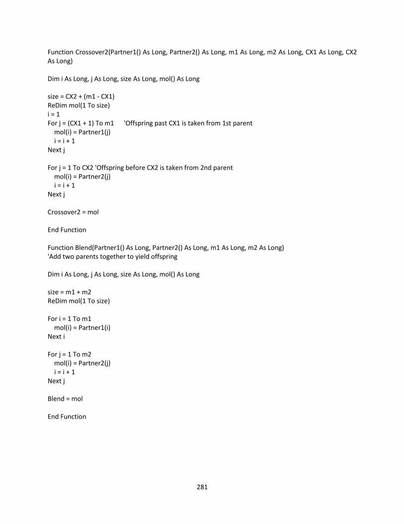
281
Function Crossover2(Partner1() As Long, Partner2() As Long, m1 As Long, m2 As Long, CX1 As Long, CX2 As Long) Dim i As Long, j As Long, size As Long, mol() As Long size = CX2 + (m1 - CX1) ReDim mol(1 To size) i = 1 For j = (CX1 + 1) To m1 'Offspring past CX1 is taken from 1st parent mol(i) = Partner1(j) i = i + 1 Next j For j = 1 To CX2 'Offspring before CX2 is taken from 2nd parent mol(i) = Partner2(j) i = i + 1 Next j Crossover2 = mol End Function Function Blend(Partner1() As Long, Partner2() As Long, m1 As Long, m2 As Long) 'Add two parents together to yield offspring Dim i As Long, j As Long, size As Long, mol() As Long size = m1 + m2 ReDim mol(1 To size) For i = 1 To m1 mol(i) = Partner1(i) Next i For j = 1 To m2 mol(i) = Partner2(j) i = i + 1 Next j Blend = mol End Function

282
E. UNIFAC-IL INTERACTION PARAMETERS
Interaction parameters for the UNIFAC-IL model described in Sections 4 and 6 are given. The interaction
parameters are used in calculation of the activity coefficient for any given binary mixture of interest.
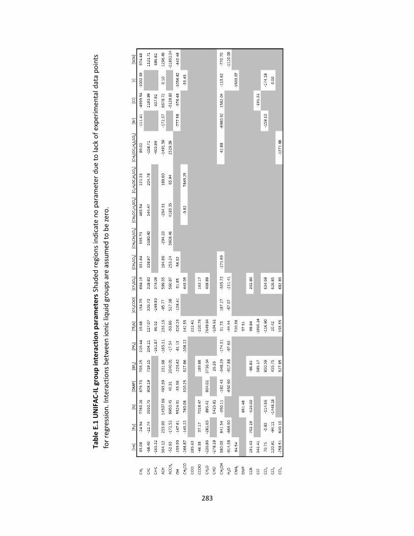
283
Tab
le E
.1 U
NIF
AC
-IL
gro
up
inte
ract
ion
par
ame
ters
Sh
aded
reg
ion
s in
dic
ate
no
par
amet
er
du
e to
lack
of
exp
erim
enta
l dat
a p
oin
ts
for
regr
essi
on
. In
tera
ctio
ns
bet
wee
n io
nic
liq
uid
gro
up
s ar
e as
sum
ed t
o b
e ze
ro.

284

285
F. SUMMARY OF EXPERIMENTAL DATA
Table F.1 summarizes the results obtained by Lavanya K. Iyer at Purdue University and used for model
development for %Monomer as a function of protein structure (Roughton, Iyer et al. 2013). All other
figures represent data obtained by the author.

286
Tab
le F
.1 S
um
mar
y o
f ex
per
ime
nta
l m
eas
ure
s o
f p
rote
in a
ggre
gati
on
via
SEC
(%
mo
no
me
r),
UV
- V
is (
AI)
an
d S
DS-
PA
GE
Val
ues
in
par
enth
esis
fo
r SE
C a
nd
A.I.
are
sta
nd
ard
err
or
abo
ut
mea
n (
SEM
) fo
r th
ree
ob
serv
atio
ns.

287
Figure F.1 Pxrd results for subset of formulations selected Each panel displays a protein–excipient pair
selected for analysis. Panels with two X-Ray diffractograms represent formulations that were chosen for
replication.

288
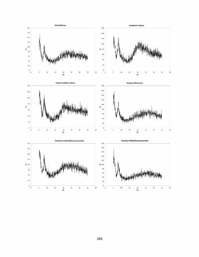
289
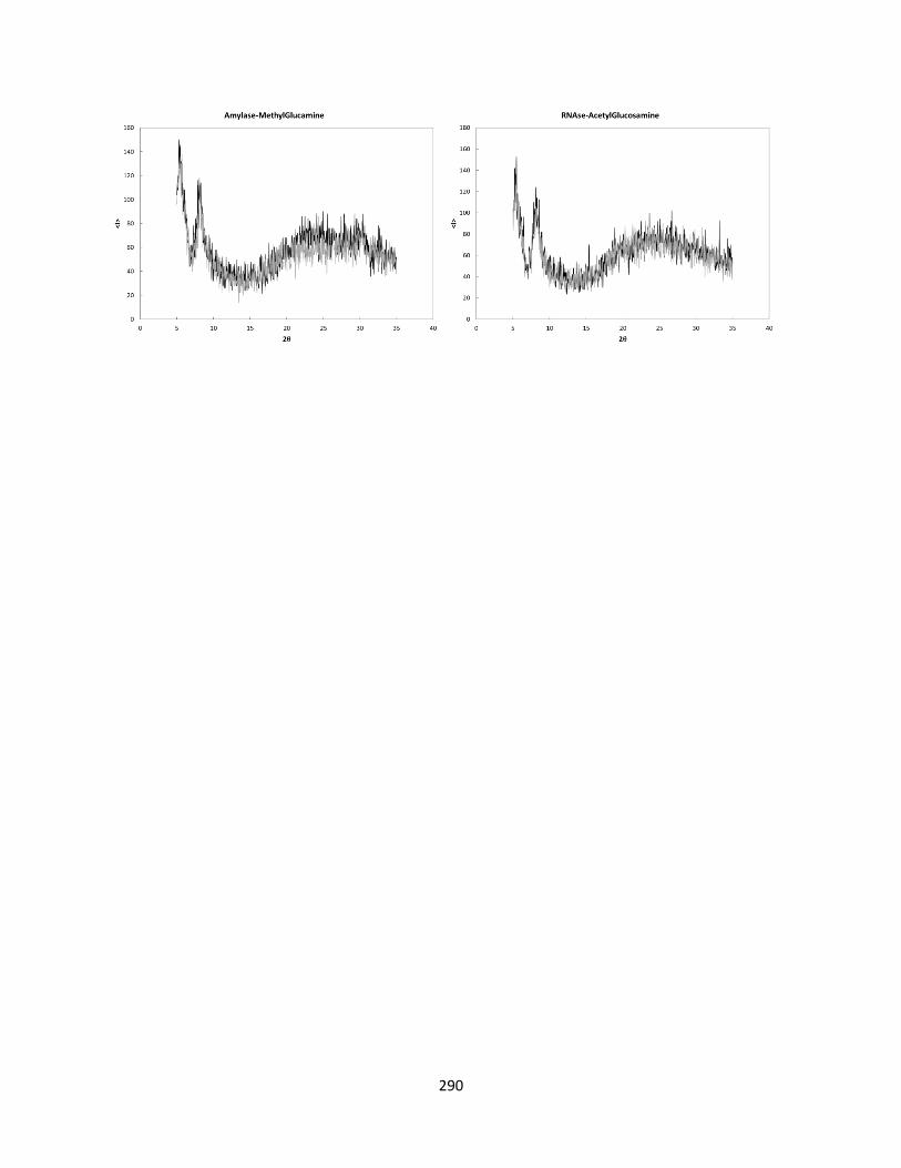
290

291
Table F.2 Experimental SEC results Value in parenthesis indicates standard error of the mean (SEM).
Excipient RNAse A BSA Ovalbumin Trypsin
Inhibitor a-Amylase
Sorbitol 99.3% (1.0%) 91.7% (1.1%) 99.6% (0.4%) 101.2% (2.1%) 98.1% (2.3%)
Mannitol 85.3% (1.7%) 82.6% (1.1%) 98.8% (0.7%) 88.9% (3.5%) 95.0% (1.2%)
Maltitol 86.6% (1.0%) 85.9% (2.3%) 92.5% (0.9%) 91.2% (0.3%) 93.5% (0.5%)
Methyl-
glucamine 89.3% (0.2%) 94.0% (0.3%) 95.2% (1.1%) 95.5% (0.8%) 97.9% (0.8%)
Glucose 99.9% (0.5%) 88.8% (0.8%) 98.4% (0.5%) 91.8% (2.1%) 99.8% (2.5%)
Mannose 85.4% (0.2%) 92.5% (1.4%) 94.8% (0.8%) 94.7% (0.6%) 98.3% (3.6%)
Methyl-
Glucopyranoside 89.2% (1.8%) 95.9% (0.6%) 95.3% (0.6%) 96.3% (0.8%)
88.2%
(10.0%)
Xylose 83.0% (1.3%) 90.6% (0.6%) 95.7% (0.6%) 93.0% (0.5%) 94.8% (2.1%)
Rhamnose 97.0% (1.7%) 85.5% (3.0%) 95.6% (0.1%) 111.1% (0.8%) 92.4% (1.3%)
Acetyl-
glucosamine 81.0% (1.7%) 92.8% (0.5%) 94.9% (0.3%) 91.6% (1.0%) 98.7% (1.2%)
Trehalose 91.5% (0.3%) 89.6% (0.6%) 98.4% (1.1%) 90.4% (0.9%) 92.1% (2.1%)
Raffinose 92.6% (1.7%) 90.8% (0.4%) 98.1% (0.5%) 86.5% (2.2%) 91.3% (4.1%)
Psicose 102.4% (2.6%) 95.1% (0.4%)
Fructose 96.0% (0.4%) 92.3% (1.4%)
2-deoxy-glucose 97.5% (0.3%) 95.1% (0.7%)
2-deoxy-ribose 88.5% (0.6%) 93.5% (0.8%)
Palatinose 98.2% (0.5%) 92.8% (1.6%)
Melibiose 96.7% (1.9%) 95.1% (0.6%)
Maltose 95.4% (0.6%) 92.8% (1.3%)
N-Acetyl-
Neuraminic Acid 95.5% (0.1%) 94.9% (1.2%)
Ethyl-glycine 96.9% (0.2%) 92.8% (1.9%)
n-acetyl-glycine 98.5% (0.4%) 93.1% (2.0%)
Gly-gly 97.7% (0.6%) 91.6% (0.4%)
Gly-leu 94.4% (0.6%) 93.4% (0.4%)
Gly-ser 97.3% (0.9%) 92.5% (0.4%)
Gly-glu 97.2% (0.6%) 88.6% (0.6%)
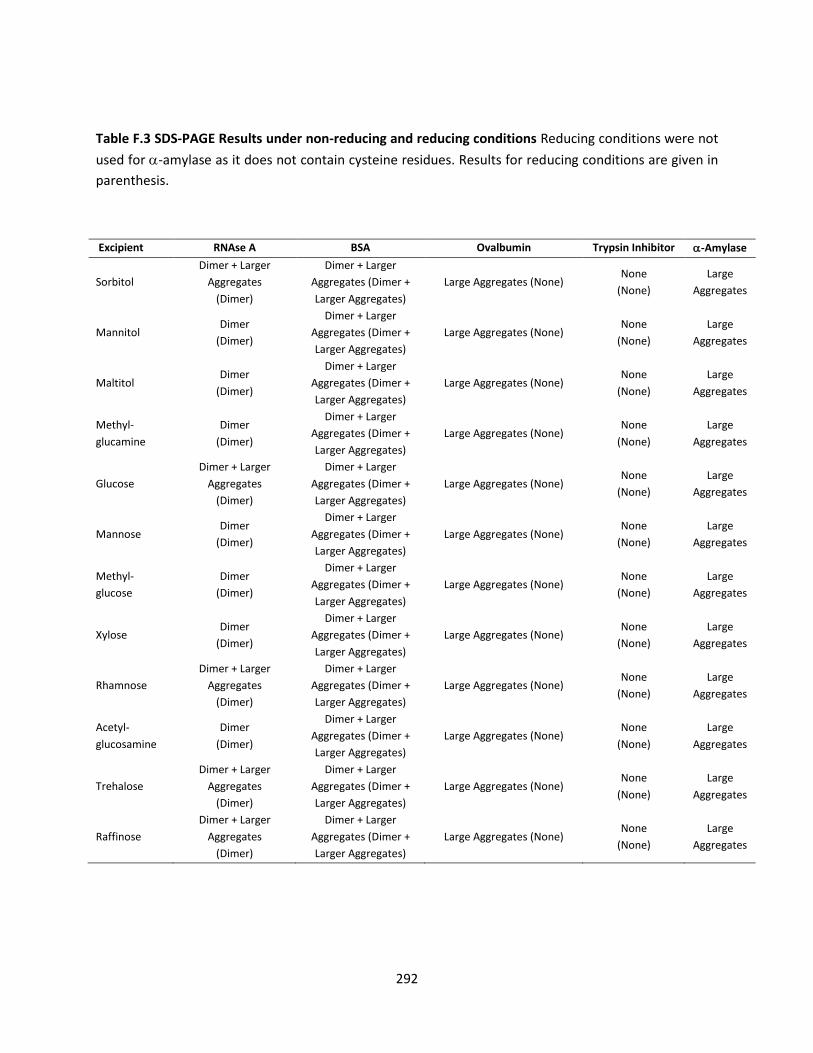
292
Table F.3 SDS-PAGE Results under non-reducing and reducing conditions Reducing conditions were not
used for -amylase as it does not contain cysteine residues. Results for reducing conditions are given in
parenthesis.
Excipient RNAse A BSA Ovalbumin Trypsin Inhibitor -Amylase
Sorbitol
Dimer + Larger
Aggregates
(Dimer)
Dimer + Larger
Aggregates (Dimer +
Larger Aggregates)
Large Aggregates (None) None
(None)
Large
Aggregates
Mannitol Dimer
(Dimer)
Dimer + Larger
Aggregates (Dimer +
Larger Aggregates)
Large Aggregates (None) None
(None)
Large
Aggregates
Maltitol Dimer
(Dimer)
Dimer + Larger
Aggregates (Dimer +
Larger Aggregates)
Large Aggregates (None) None
(None)
Large
Aggregates
Methyl-
glucamine
Dimer
(Dimer)
Dimer + Larger
Aggregates (Dimer +
Larger Aggregates)
Large Aggregates (None) None
(None)
Large
Aggregates
Glucose
Dimer + Larger
Aggregates
(Dimer)
Dimer + Larger
Aggregates (Dimer +
Larger Aggregates)
Large Aggregates (None) None
(None)
Large
Aggregates
Mannose Dimer
(Dimer)
Dimer + Larger
Aggregates (Dimer +
Larger Aggregates)
Large Aggregates (None) None
(None)
Large
Aggregates
Methyl-
glucose
Dimer
(Dimer)
Dimer + Larger
Aggregates (Dimer +
Larger Aggregates)
Large Aggregates (None) None
(None)
Large
Aggregates
Xylose Dimer
(Dimer)
Dimer + Larger
Aggregates (Dimer +
Larger Aggregates)
Large Aggregates (None) None
(None)
Large
Aggregates
Rhamnose
Dimer + Larger
Aggregates
(Dimer)
Dimer + Larger
Aggregates (Dimer +
Larger Aggregates)
Large Aggregates (None) None
(None)
Large
Aggregates
Acetyl-
glucosamine
Dimer
(Dimer)
Dimer + Larger
Aggregates (Dimer +
Larger Aggregates)
Large Aggregates (None) None
(None)
Large
Aggregates
Trehalose
Dimer + Larger
Aggregates
(Dimer)
Dimer + Larger
Aggregates (Dimer +
Larger Aggregates)
Large Aggregates (None) None
(None)
Large
Aggregates
Raffinose
Dimer + Larger
Aggregates
(Dimer)
Dimer + Larger
Aggregates (Dimer +
Larger Aggregates)
Large Aggregates (None) None
(None)
Large
Aggregates